replacement and richness difference - université de...

Partitioning BD into replacement and richness difference

Pierre LegendreDépartement de sciences biologiques

Université de Montréalhttp://www.NumericalEcology.com/

© Pierre Legendre 2017

1. Whittaker’s alpha, beta and gamma diversities2. Compute total beta diversity (BDTotal)3. Partitioning D into Repl and RichDiff components4. Case study: Doubs River fish data5. Conclusion6. References

Outline of the presentation

Replacement and Richness difference

• Alpha diversity is local diversity –or species diversity at a site. Estimated by species richness or by one of the alpha diversity indices (richness, Shannon, Simpson).• Beta diversity is spatial differentiation –or the variation in species composition among sites within a region of interest. • Gamma diversity is regional diversity –or species diversity in a region of interest. Estimated by pooling observations from a large number of sites in the area and computing an alpha diversity index.Robert Whittaker (1960, 1972).

1. Alpha, beta and gamma diversities

Species

Sites

=> αi= N0, H1, N2, ...1

23...

n

Sums => γ = N0, H1, N2, ...

=>

1 2 3 . . . p

β = variation inspecies compositionamong sites

Diversity levels

Y = communitycomposition

data

Legendre & Legendre Numerical ecology (2012, Fig. 6.3).

Dnxn

Species contributionsto beta diversity (SCBD)

Local contributionsto beta diversity (LCBD)

1 ... p

1 ... n

Ytr. nxp

Transformedspecies

composition

Snxp

Squareddifferences fromcolumn means

Dissimilarities amongsampling units

(1) (3)

(6b)

(6a)

(2)

(5)

(4)

(7)

SSTotal

BDTotal

(8)(10)

Totaldispersion

Total betadiversity

Ynxp

Speciescomposition

2. Compute total beta diversity (BDTotal)


=> Partition the dissimilarities D into Replacement and Richness difference components.

Two different methods have been proposed:

(1)  by Baselga (in Spain) and

(2)  by Podani (in Hungary) and coauthors.

Each group proposed ways of partitioning the Jaccard and Sørensen dissimilarity indices for presence-absence data, as well as their quantitative forms, the Ružička and percentage difference indices.

=> I will focus on the Podani approach. I will describe how these new indices can be interpreted through graphical analysis.

3. Partitioning D into Repl and RichDiff

The dissimilarity D between two sites contains two components:

• replacement (turnover): environmental gradients, competition …

• and richness difference due to difference in diversity of niches causing species thinning, or other processes (e.g. physical barriers).

! " #

$%&'()"*#+

,"-#,

./01!#/&/(2

.'#3(/44 5'66/7/(#/

8'44'&'1!7'29 ":#

;<&0<(/(24<6 !

"!(5 !

#

='2/ >

='2/ $


Podani-family indices, presence-absence data

! " #

$%&'()"*#+

,"-#,

./01!#/&/(2

.'#3(/44 5'66/7/(#/

8'44'&'1!7'29 ":#

;<&0<(/(24<6 !

"!(5 !

#

='2/ >

='2/ $


! " #

$%&'()"*#+

,"-#,

./01!#/&/(2

.'#3(/44 5'66/7/(#/

8'44'&'1!7'29 ":#

;<&0<(/(24<6 !

"!(5 !

#

='2/ >

='2/ $

Podani-family indice, species abundance data

Spec.1 Spec.4Spec.3Spec.2

Site1 Site2 Site1 Site2 Site1 Site2 Site1 Site2

A = abun. common to sites 1 and 2 = A1+A2+0+A4B = abundances unique to site 1 = 0+B2+B3+0C = abundances unique to site 2 = C1+0+0+0

A1 A1 A2 A2

A4 A4B2

B3

C1

Spec.1 Spec.4Spec.3Spec.2

Site1 Site2 Site1 Site2 Site1 Site2 Site1 Site2

A = abun. common to sites 1 and 2 = A1+A2+0+A4B = abundances unique to site 1 = 0+B2+B3+0C = abundances unique to site 2 = C1+0+0+0

A1 A1 A2 A2

A4 A4B2

B3

C1

Fish observed at 29 sites along the Doubs river, a tributary of the

Saône River running near the France-Switzerland border in the Jura

Mountains in eastern France.

• Data from Verneaux (1973), available on the Web page of the book

Numerical ecology with R (Borcard et al. 2011):

http://adn.biol.umontreal.ca/~numericalecology/numecolR/

4. Case study: Doubs River fish data


http://fr.wikipedia.org/wiki/Doubs_(rivière) Les sources du Doubs à Mouthe

Besançon

Entre Laissey et Deluz, peu avant Besançon

Decomposing dissimilarity matrices

D


Repl

Replacementamong sampling units

RichDiff

Richness differenceamong sampling units

Repl + RichDiff = D

D


Repl


RichDiff


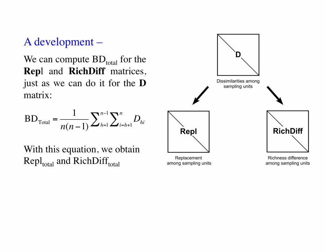
A development –We can compute BDtotal for the Repl and RichDiff matrices, just as we can do it for the D matrix:

BDTotal =1

n(n−1)Dhii=h+1

n∑h=1

n−1∑

With this equation, we obtain Repltotal and RichDifftotal

D


Repl


RichDiff


• In the Podani family of indices used in the examples (below), the partitioning is additive: BTtotal(Repl) + BDtotal(RichDiff) = BDtotal(D).

• In the Baselga family (not developed further in this talk), RichDiff is replaced by Nestedness (Nes). The partitioning is not additive: BDtotal(Repl) + BDtotal(Nes) ≠ BDtotal(D).

Decomposition of the fish beta diversityfor presence-absence data, Podani family

=> Beta diversity in the Doubs River is dominated by richness differences among sites


Jaccard Sørensen

BDTotal 0.326 0.267

BDmax = 0.5 65% of BDmax 53% of BDmax

ReplTotal / BDTotal 0.28 0.28

RichDiffTotal / BDTotal 0.72 0.72

(a) Jaccard dissimilarity (D, ), replacement ( ) and richness difference ( ) indices for presence-absence data: sites 1–29 are compared to site 30. (b) Species richness. Grey: polluted #23 to 25.

Indices computed from site 30 (confluence site), presence-absence data= Jaccard D, = replacement, = richness difference

D=Jaccard

!"#

1 2 3 4 5 6 7 9 10 11 12 13 14 15 16 17 18 19 20 21 22 23 24 25 26 27 28 29 30

Referencesite

0.0

0.2

0.4

0.6

0.8

1.0

05

10152025

Species richness

Sites (site #8 removed)

Speciesrichness

!$#

Upstream Downstream

1 2 3 4 5 6 7 9 10 11 12 13 14 15 16 17 18 19 20 21 22 23 24 25 26 27 28 29 30

-0.4 -0.2 0.0 0.2 0.4 0.6

-0.4

-0.2

0.0

0.2

0.4

0.6

Axis 1

Axis2

1

2

34

567

9

10

11 12

13 14 1516 17

18

19

20 2122,27,28

23

2425

26

29

30

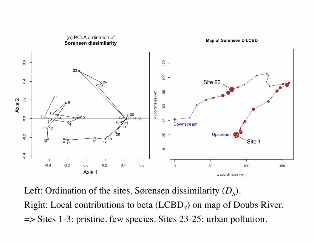
(a) PCoA ordination ofSorensen dissimilarity

Left: Ordination of the sites, Sørensen dissimilarity (DS).Right: Local contributions to beta (LCBDS) on map of Doubs River.=> Sites 1-3: pristine, few species. Sites 23-25: urban pollution.

0 50 100 1500

2040

6080

100

120

Map of Sørensen D LCBD

x coordinates (km)

y co

ordi

nate

s (k

m)

Upstream

Downstream

Site 1"

Site 23"

-0.4 -0.2 0.0 0.2 0.4 0.6

-0.4

-0.2

0.0

0.2

0.4

Axis 1

Axis2

-0.4 -0.2 0.0 0.2 0.4

-0.2

0.0

0.2

0.4

0.6

Axis 1Axis2

1

2

3

45

6

79

10

11,12

1314

15

16

17 18

192021

22,27,28

23

24

2526

29

30

(b) PCoA ordination ofReplacement (ReplS)

1

2

3

4,24,25

5,156,14

7,9

10-13

16

17,20,22,27,28

18,19,21

23

26,30

29

(c) PCoA ordination ofRichness difference (RichDiffS)

Left: Ordination of the sites, ReplS (28% of beta diversity).Right: Replacement LCBD (ReplLCBD) on map of Doubs River.=> Higher replacement LCBD at sites 11-15 and 23-25.

0 50 100 1500

2040

6080

100

120

Map of Replacement LCBD

x coordinates (km)

y co

ordi

nate

s (k

m)

Upstream

Downstream

Site 23"

Site 1"

-0.4 -0.2 0.0 0.2 0.4 0.6

-0.4

-0.2

0.0

0.2

0.4

Axis 1

Axis2

-0.4 -0.2 0.0 0.2 0.4

-0.2

0.0

0.2

0.4

0.6

Axis 1

Axis2

1

2

3

45

6

79

10

11,12

1314

15

16

17 18

192021

22,27,28

23

24

2526

29

30

(b) PCoA ordination ofReplacement (ReplS)

1

2

3

4,24,25

5,156,14

7,9

10-13

16

17,20,22,27,2818,19,21

2326,3029

(c) PCoA ordination ofRichness difference (RichDiffS)

Left: Ordination of the sites, RichDiffS (72% of beta diversity).Right: Richness difference LCBD (RichDiffLCBD) on Doubs River map.=> Higher richness difference LCBD at sites 1-3 and 23.

0 50 100 1500

2040

6080

100

120

Map of Richness difference LCBD

x coordinates (km)

y co

ordi

nate

s (k

m)

Upstream

Downstream

Site 1"

Site 23"

R code: beta diversity partitioning, Doubs River fish data

# Load the Doubs.RData file !# Data frame "spe" contains the fish data (30 sites x 27 species)!

spe <- spe[-8,] # Remove site 8 were no fish were caught!

# Compute partitioning with function beta.div.comp() of adepsatial!

res1 <- beta.div.comp(spe, coef="S", quant=FALSE) # Sørensen coeff. !

summary(res1) # Examine the structure of the output file!

res1$part!

BDtotal Repl RichDif Repl/BDtotal RichDif/BDtotal !0.26738159 0.07557385 0.19180774 0.28264417 0.71735583 !

Compare the results in this vector to the Doubs River results computed with the Sørensen index, shown 5 slides back.

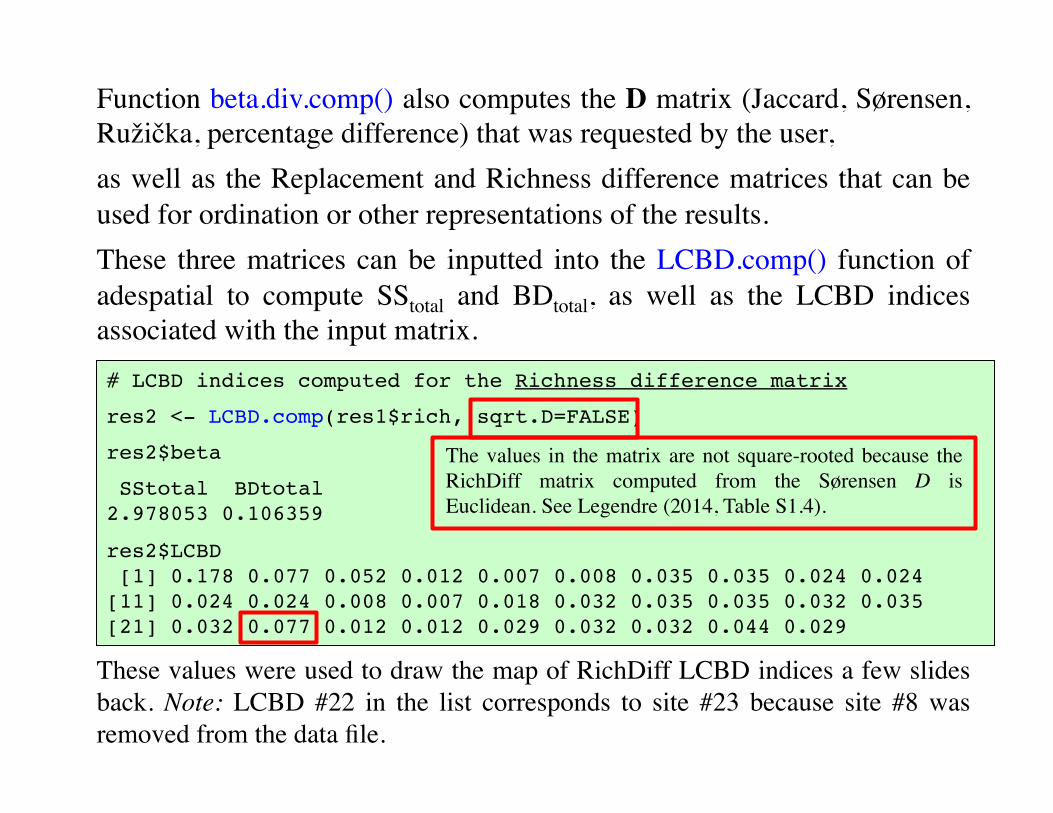
Function beta.div.comp() also computes the D matrix (Jaccard, Sørensen, Ružička, percentage difference) that was requested by the user, as well as the Replacement and Richness difference matrices that can be used for ordination or other representations of the results.These three matrices can be inputted into the LCBD.comp() function of adespatial to compute SStotal and BDtotal, as well as the LCBD indices associated with the input matrix.# LCBD indices computed for the Richness difference matrix !

res2 <- LCBD.comp(res1$rich, sqrt.D=FALSE) !

res2$beta!

SStotal BDtotal !2.978053 0.106359 !

res2$LCBD! [1] 0.178 0.077 0.052 0.012 0.007 0.008 0.035 0.035 0.024 0.024 ![11] 0.024 0.024 0.008 0.007 0.018 0.032 0.035 0.035 0.032 0.035 ![21] 0.032 0.077 0.012 0.012 0.029 0.032 0.032 0.044 0.029!

The values in the matrix are not square-rooted because the RichDiff matrix computed from the Sørensen D is Euclidean. See Legendre (2014, Table S1.4).

These values were used to draw the map of RichDiff LCBD indices a few slides back. Note: LCBD #22 in the list corresponds to site #23 because site #8 was removed from the data file.

Test a hypothesis about the response of community data to a factor

=> This analysis could be carried out with an experimental factor.

The environmental data were used to classify the sites in two groups (Ward clustering): sites 1-22 (upper course) and 23-30 (lower course).

The DJ, ReplJ and RichDiffJ matrices were tested against this classification using McArdle & Anderson’s (2001) F-test in RDA for non-Euclidean matrices. Function dbrda() in vegan was used.

Results –DJ was significantly explained by the classification (p = 0.005)ReplJ was significantly explained by the classification (p = 0.001)RichDiffJ was not significantly explained by the classif. (p = 0.943)

Identify the environmental factorsresponsible for variation in the matrices

=> The two components, ReplJ and RichDiffJ, are influenced by different environmental processes, which all influence DJ.

The DJ, ReplJ and RichDiffJ matrices were transformed into rectangular data matrices by principal coordinate analysis (PCoA).

Environmental variables that significantly explained the variation in each matrix were selected (forward selection).

Results –DJ – was explained by {slope, hardness, nitrate, O2}ReplJ was explained by {O2}RichDiffJ was explained by {slope, hardness, nitrate}

Other methods of graphical analysis have been suggested – for example the triangular plots proposed by Podani & Schmera (2011) and Podani et al. (2013).

The analysis of the Doubs River fish data using triangular plots is shown in the paper.


Replacement and richness difference indices can be interpreted and related to ecosystem processes.

Innovations in the Legendre (2014) paper –

• The index values can be summed across all pairs of sites; these sums decompose total beta diversity into total replacement and total richness difference components.

• Local contributions of replacement and richness difference to total beta diversity can be computed and mapped.

• Within a region, differences among sites measured by these indices can be analysed and interpreted using explanatory variables.

• Replacement and richness difference matrices can be analysed by all methods of multivariate data analysis for dissimilarity matrices.

5. Conclusion

6. References

Baselga, A. 2010. Partitioning the turnover and nestedness components of beta diversity. Global Ecology and Biogeography 19: 134–143.

Baselga, A. 2012. The relationship between species replacement, dissimilarity derived from nestedness, and nestedness. Global Ecology and Biogeography 21: 1223–1232.

Baselga, A. 2013. Separating the two components of abundance-based dissimilarity: balanced changes in abundance vs. abundance gradients. Methods in Ecology and Evolution 4: 552– 557.

Cardoso, P., P. A. V. Borges & J. A. Veech. 2009. Testing the performance of beta diversity measures based on incidence data: the robustness to undersampling. Diversity and Distributions 15: 1081–1090.

Carvalho, J. C., P. Cardoso, P. A. V. Borges, D. Schmera & J. Podani. 2013. Measuring fractions of beta diversity and their relationships to nestedness: a theoretical and empirical comparison of novel approaches. Oikos 122: 825–834.

Legendre, P. 2014. Interpreting the replacement and richness difference components of beta diversity. Global Ecology and Biogeography 23: 1324-1334.

Podani, J., C. Ricotta & D. Schmera. 2013. A general framework for analyzing beta diversity, nestedness and related community-level phenomena based on abundance data. Ecological Complexity 15: 52–61.

Podani, J. & D. Schmera. 2011. A new conceptual and methodological framework for exploring and explaining pattern in presence-absence data. Oikos 120: 1625–1638.

End of section


replacement and richness difference - université de...

Documents