report 1 make digital filters run faster - stefan...
TRANSCRIPT
1 Embedded Systems – WS 2014/15 – „Report 1: Make digital filters run faster“ – Stefan Feilmeier
Facultatea de Inginerie Hermann Oberth Master-Program “Embedded Systems“ Advanced Digital Signal Processing Methods Winter Semester 2014/2015
Report 1
Make digital filters run faster
Professor: Prof. dr. ing. Mihu Ioan
Masterand: Stefan Feilmeier
05.01.2015
2 Embedded Systems – WS 2014/15 – „Report 1: Make digital filters run faster“ – Stefan Feilmeier
TABLE OF CONTENTS
1 Overview 3
1.1 Digital filters 3
1.2 Digital Transforms 3
2 The goal of this paper 4
3 Faster Filter Algorithms 4
3.1 Decimation 4
3.2 FIR Filter Structure 6
3.2.1 Direct-form FIR structure (tapped delay line) 7
3.2.2 Symmetric direct-form FIR structure. 7
3.2.3 Transposed direct-form FIR structure 8
3.3 IIR Filter Structure 9
3.3.1 Direct-form IIR structure 9
4 Faster microcontroller 9
4.1 Criteria related to microcontroller architecture 9
4.2 Criteria related to the speed of calculation 11
4.3 Economic criteria 14
4.4 Digital Signal Processor. 14
5 Faster type of computation 16
5.1 Fixed point vs floating point 16
6 Programming techniques 17
6.1 Look Up Table (LUT) 17
6.2 Programming Language 18
6.3 Avoiding slow functions 18
Table of Figures 20
Table of Equations 20
Note: This report is based on a Template by Prof. dr. ing. Mihu Ioan. Contents with background colour
were added by Stefan Feilmeier.
3 Embedded Systems – WS 2014/15 – „Report 1: Make digital filters run faster“ – Stefan Feilmeier
1 OVERVIEW
In this document, we will be focused on the most important algorithms used in DSP:
1.1 DIGITAL FILTERS
x[n] y[n] Filter
algorithm
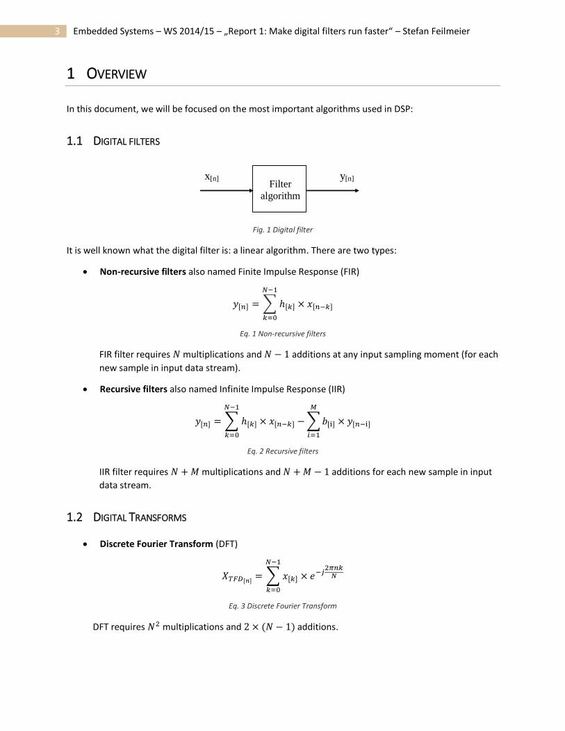
Fig. 1 Digital filter
It is well known what the digital filter is: a linear algorithm. There are two types:
Non-recursive filters also named Finite Impulse Response (FIR)
𝑦[𝑛] = ∑ ℎ[𝑘] × 𝑥[𝑛−𝑘]
𝑁−1
𝑘=0
Eq. 1 Non-recursive filters
FIR filter requires 𝑁 multiplications and 𝑁 − 1 additions at any input sampling moment (for each
new sample in input data stream).
Recursive filters also named Infinite Impulse Response (IIR)
𝑦[𝑛] = ∑ ℎ[𝑘] × 𝑥[𝑛−𝑘] − ∑ 𝑏[i] × 𝑦[𝑛−i]
𝑀
𝑖=1
𝑁−1
𝑘=0
Eq. 2 Recursive filters
IIR filter requires 𝑁 + 𝑀 multiplications and 𝑁 + 𝑀 − 1 additions for each new sample in input
data stream.
1.2 DIGITAL TRANSFORMS
Discrete Fourier Transform (DFT)
𝑋𝑇𝐹𝐷[𝑛]= ∑ 𝑥[𝑘] × 𝑒−𝑗
2𝜋𝑛𝑘𝑁
𝑁−1
𝑘=0
Eq. 3 Discrete Fourier Transform
DFT requires 𝑁2 multiplications and 2 × (𝑁 − 1) additions.
4 Embedded Systems – WS 2014/15 – „Report 1: Make digital filters run faster“ – Stefan Feilmeier
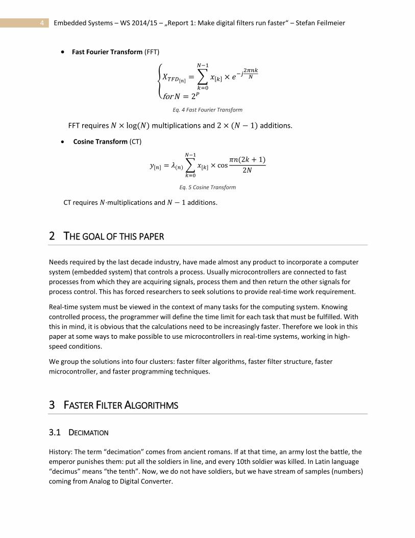
Fast Fourier Transform (FFT)
{𝑋𝑇𝐹𝐷[𝑛]
= ∑ 𝑥[𝑘] × 𝑒−𝑗2𝜋𝑛𝑘
𝑁
𝑁−1
𝑘=0
for 𝑁 = 2𝑃
Eq. 4 Fast Fourier Transform
FFT requires 𝑁 × log(𝑁) multiplications and 2 × (𝑁 − 1) additions.
Cosine Transform (CT)
𝑦[𝑛] = 𝜆(𝑛) ∑ 𝑥[𝑘] × cos𝜋𝑛(2𝑘 + 1)
2𝑁
𝑁−1
𝑘=0
Eq. 5 Cosine Transform
CT requires 𝑁·multiplications and 𝑁 − 1 additions.
2 THE GOAL OF THIS PAPER
Needs required by the last decade industry, have made almost any product to incorporate a computer
system (embedded system) that controls a process. Usually microcontrollers are connected to fast
processes from which they are acquiring signals, process them and then return the other signals for
process control. This has forced researchers to seek solutions to provide real-time work requirement.
Real-time system must be viewed in the context of many tasks for the computing system. Knowing
controlled process, the programmer will define the time limit for each task that must be fulfilled. With
this in mind, it is obvious that the calculations need to be increasingly faster. Therefore we look in this
paper at some ways to make possible to use microcontrollers in real-time systems, working in high-
speed conditions.
We group the solutions into four clusters: faster filter algorithms, faster filter structure, faster
microcontroller, and faster programming techniques.
3 FASTER FILTER ALGORITHMS
3.1 DECIMATION
History: The term “decimation” comes from ancient romans. If at that time, an army lost the battle, the
emperor punishes them: put all the soldiers in line, and every 10th soldier was killed. In Latin language
“decimus” means “the tenth”. Now, we do not have soldiers, but we have stream of samples (numbers)
coming from Analog to Digital Converter.
5 Embedded Systems – WS 2014/15 – „Report 1: Make digital filters run faster“ – Stefan Feilmeier
In this context, we shall find reason to eliminate some sample from the stream. Not always the tenth,
but depending on context, can be removed the second, the third, or more complicated rules can be used
to eliminate samples. Nevertheless, today the term “decimation” is used in all these cases of removing
samples.
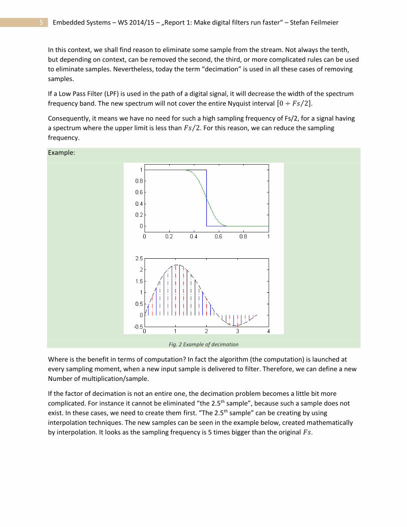
If a Low Pass Filter (LPF) is used in the path of a digital signal, it will decrease the width of the spectrum
frequency band. The new spectrum will not cover the entire Nyquist interval [0 ÷ 𝐹𝑠 2⁄ ].
Consequently, it means we have no need for such a high sampling frequency of Fs/2, for a signal having
a spectrum where the upper limit is less than 𝐹𝑠 2⁄ . For this reason, we can reduce the sampling
frequency.
Example:
Fig. 2 Example of decimation
Where is the benefit in terms of computation? In fact the algorithm (the computation) is launched at
every sampling moment, when a new input sample is delivered to filter. Therefore, we can define a new
Number of multiplication/sample.
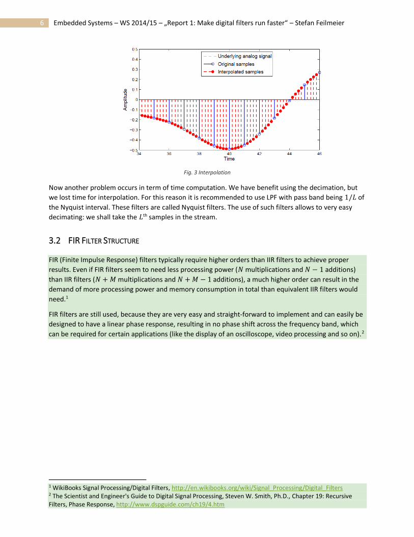
If the factor of decimation is not an entire one, the decimation problem becomes a little bit more
complicated. For instance it cannot be eliminated “the 2.5th sample”, because such a sample does not
exist. In these cases, we need to create them first. “The 2.5th sample” can be creating by using
interpolation techniques. The new samples can be seen in the example below, created mathematically
by interpolation. It looks as the sampling frequency is 5 times bigger than the original 𝐹𝑠.
6 Embedded Systems – WS 2014/15 – „Report 1: Make digital filters run faster“ – Stefan Feilmeier
Fig. 3 Interpolation
Now another problem occurs in term of time computation. We have benefit using the decimation, but
we lost time for interpolation. For this reason it is recommended to use LPF with pass band being 1/𝐿 of
the Nyquist interval. These filters are called Nyquist filters. The use of such filters allows to very easy
decimating: we shall take the 𝐿th samples in the stream.
3.2 FIR FILTER STRUCTURE
FIR (Finite Impulse Response) filters typically require higher orders than IIR filters to achieve proper
results. Even if FIR filters seem to need less processing power (𝑁 multiplications and 𝑁 − 1 additions)
than IIR filters (𝑁 + 𝑀 multiplications and 𝑁 + 𝑀 − 1 additions), a much higher order can result in the
demand of more processing power and memory consumption in total than equivalent IIR filters would
need.1
FIR filters are still used, because they are very easy and straight-forward to implement and can easily be
designed to have a linear phase response, resulting in no phase shift across the frequency band, which
can be required for certain applications (like the display of an oscilloscope, video processing and so on).2
1 WikiBooks Signal Processing/Digital Filters, http://en.wikibooks.org/wiki/Signal_Processing/Digital_Filters 2 The Scientist and Engineer's Guide to Digital Signal Processing, Steven W. Smith, Ph.D., Chapter 19: Recursive Filters, Phase Response, http://www.dspguide.com/ch19/4.htm
7 Embedded Systems – WS 2014/15 – „Report 1: Make digital filters run faster“ – Stefan Feilmeier
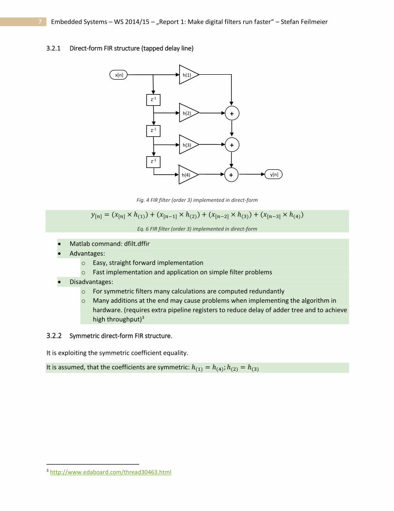
3.2.1 Direct-form FIR structure (tapped delay line)
Fig. 4 FIR filter (order 3) implemented in direct-form
𝑦[𝑛] = (𝑥[𝑛] × ℎ(1)) + (𝑥[𝑛−1] × ℎ(2)) + (𝑥[𝑛−2] × ℎ(3)) + (𝑥[𝑛−3] × ℎ(4))
Eq. 6 FIR filter (order 3) implemented in direct-form
Matlab command: dfilt.dffir
Advantages:
o Easy, straight forward implementation
o Fast implementation and application on simple filter problems
Disadvantages:
o For symmetric filters many calculations are computed redundantly
o Many additions at the end may cause problems when implementing the algorithm in
hardware. (requires extra pipeline registers to reduce delay of adder tree and to achieve
high throughput)3
3.2.2 Symmetric direct-form FIR structure.
It is exploiting the symmetric coefficient equality.
It is assumed, that the coefficients are symmetric: ℎ(1) = ℎ(4); ℎ(2) = ℎ(3)
3 http://www.edaboard.com/thread30463.html
z-1
+
h(1)
z-1
z-1
h(2)
h(3)
h(4)
+
+ y[n]
x[n]
8 Embedded Systems – WS 2014/15 – „Report 1: Make digital filters run faster“ – Stefan Feilmeier
Fig. 5 FIR filter (order 3) implemented in symmetric direct-form
𝑦[𝑛] = [(𝑥[𝑛] × ℎ(1)) + (𝑥[𝑛−3] × ℎ(1))] + [(𝑥[𝑛−1] × ℎ(2)) + (𝑥[𝑛−2] × ℎ(2))]
Eq. 7 FIR filter (order 3) implemented in symmetric direct-form
Matlab command: dfilt.dfsymfir
Advantage:
o Less computing power required
Disadvantage:
o Increased algorithm complexity
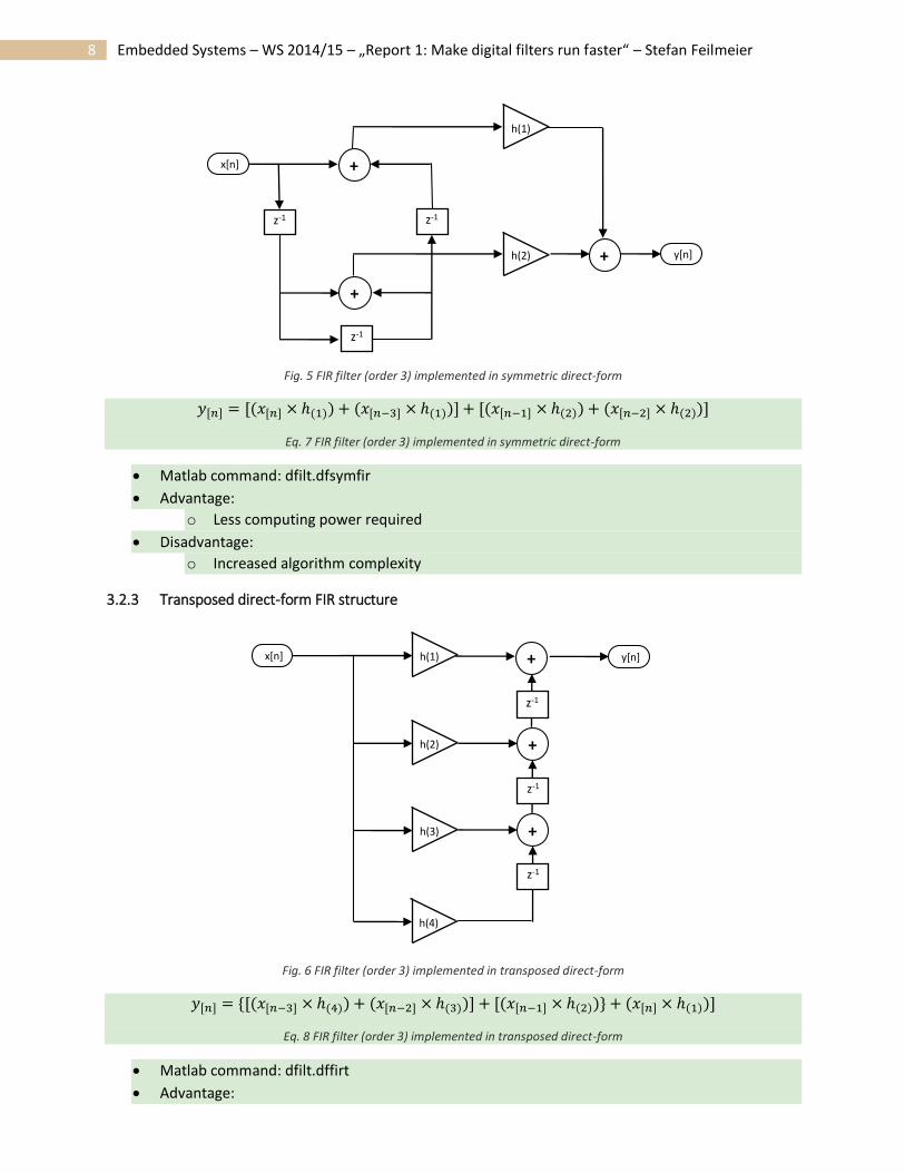
3.2.3 Transposed direct-form FIR structure
Fig. 6 FIR filter (order 3) implemented in transposed direct-form
𝑦[𝑛] = {[(𝑥[𝑛−3] × ℎ(4)) + (𝑥[𝑛−2] × ℎ(3))] + [(𝑥[𝑛−1] × ℎ(2))} + (𝑥[𝑛] × ℎ(1))]
Eq. 8 FIR filter (order 3) implemented in transposed direct-form
Matlab command: dfilt.dffirt
Advantage:
z-1 z-1
z-1
+
+
x[n]
+
h(1)
h(2) y[n]
z-1
+
h(1)
h(2)
h(3)
h(4)
+
y[n] x[n] +
z-1
z-1
9 Embedded Systems – WS 2014/15 – „Report 1: Make digital filters run faster“ – Stefan Feilmeier
o Easier and faster implementation in hardware (many small additions in contrast to one
big addition at the end)
3.3 IIR FILTER STRUCTURE
IIR (Infinite Impulse Response) can provide higher quality filters, requiring less computations and less
memory consumption compared to FIR filters. But because of the internal feedback mechanism, linear
response phase is not easily achieved and the feedback can also cause problems in finite-precision
arithmetic, as inaccuracies are carried forward.
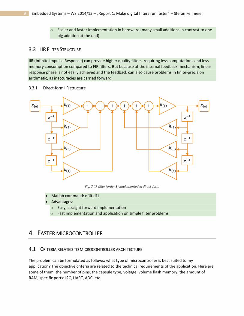
3.3.1 Direct-form IIR structure
Fig. 7 IIR filter (order 3) implemented in direct-form
Matlab command: dfilt.df1
Advantages:
o Easy, straight forward implementation
o Fast implementation and application on simple filter problems
4 FASTER MICROCONTROLLER
4.1 CRITERIA RELATED TO MICROCONTROLLER ARCHITECTURE
The problem can be formulated as follows: what type of microcontroller is best suited to my
application? The objective criteria are related to the technical requirements of the application. Here are
some of them: the number of pins, the capsule type, voltage, volume flash memory, the amount of
RAM, specific ports: I2C, UART, ADC, etc.
𝑥[𝑛]
𝑏(2)
𝑏(1)
𝑏(3)
𝑏(4)
+ + + + + +
ℎ(2)
ℎ(1)
ℎ(3)
ℎ(4)
𝑧−1
𝑧−1
𝑧−1
𝑥[𝑛]
𝑧−1
𝑧−1
𝑧−1
10 Embedded Systems – WS 2014/15 – „Report 1: Make digital filters run faster“ – Stefan Feilmeier
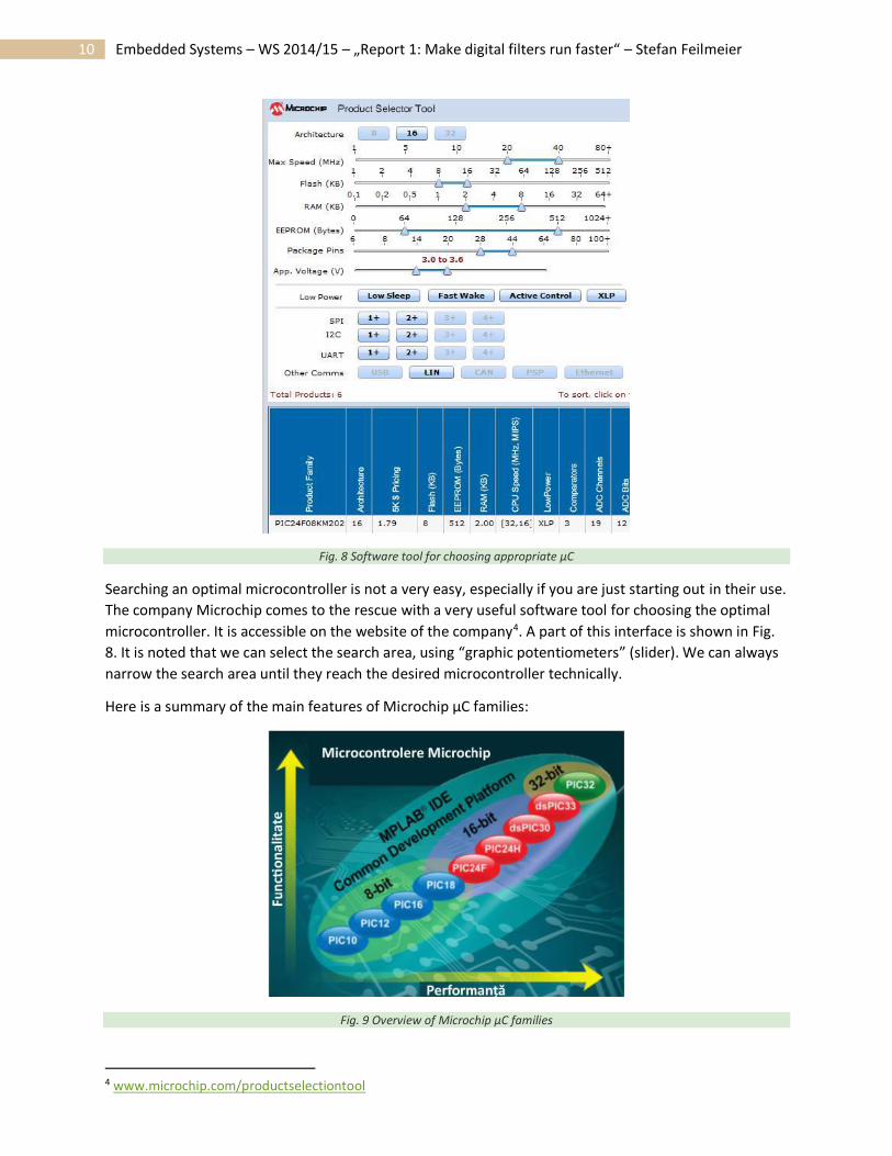
Fig. 8 Software tool for choosing appropriate μC
Searching an optimal microcontroller is not a very easy, especially if you are just starting out in their use.
The company Microchip comes to the rescue with a very useful software tool for choosing the optimal
microcontroller. It is accessible on the website of the company4. A part of this interface is shown in Fig.
8. It is noted that we can select the search area, using “graphic potentiometers” (slider). We can always
narrow the search area until they reach the desired microcontroller technically.
Here is a summary of the main features of Microchip μC families:
Fig. 9 Overview of Microchip μC families
4 www.microchip.com/productselectiontool
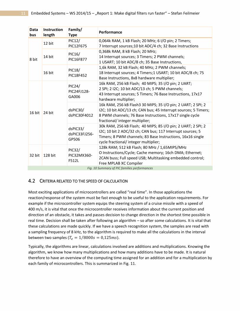
11 Embedded Systems – WS 2014/15 – „Report 1: Make digital filters run faster“ – Stefan Feilmeier
Data bus
Instruction length
Family/ Type
Performance
8 bit
12 bit PIC12/ PIC12F675
0,064k RAM, 1 kB Flash; 20 MHz; 6 I/O pin; 2 Timers; 7 Interrupt sources;10 bit ADC/4 ch; 32 Base Instructions
14 bit PIC16/ PIC16F877
0,368k RAM, 8 kB Flash; 20 MHz; 14 Interrupt sources; 3 Timers; 2 PWM channels; 1 USART; 10 bit ADC/8 ch; 35 Base Instructions,
16 bit PIC18/ PIC18F452
1,6k RAM, 32 kB Flash; 40 MHz; 2 PWM channels; 18 Interrupt sources; 4 Timers;1 USART; 10 bit ADC/8 ch; 75 Base Instructions, 8x8 hardware multiplier;
16 bit 24 bit
PIC24/ PIC24FJ128- GA006
16k RAM, 256 kB Flash; 40 MIPS; 35 I/O pin; 2 UART; 2 SPI; 2 I2C; 10 bit ADC/13 ch; 5 PWM channels; 43 Interrupt sources; 5 Timers; 76 Base Instructions, 17x17 hardware multiplier;
dsPIC30/ dsPIC30F4012
16k RAM, 256 kB Flash3 30 MIPS; 35 I/O pin; 2 UART; 2 SPI; 2 I2C; 10 bit ADC/13 ch; CAN bus; 45 Interrupt sources; 5 Timers; 8 PWM channels; 76 Base Instructions, 17x17 single cycle fractional/ integer multiplier;
dsPIC33/ dsPIC33FJ256-GP506
30k RAM, 256 kB Flash; 40 MIPS; 85 I/O pin; 2 UART; 2 SPI; 2 I2C; 10 bit 2 ADC/32 ch; CAN bus; 117 Interrupt sources; 5 Timers; 8 PWM channels; 83 Base Instructions, 16x16 single cycle fractional/ integer multiplier;
32 bit 128 bit PIC32/ PIC32MX360-F512L
128k RAM; 512 kB Flash; 80 MHz / 1,65MIPS/MHz O Instructions/Cycle; Cache memory; 16ch DMA; Ethernet; 2CAN buss; Full speed USB; Multitasking embedded control; Free MPLAB XC Compiler
Fig. 10 Summary of PIC families performances
4.2 CRITERIA RELATED TO THE SPEED OF CALCULATION
Most exciting applications of microcontrollers are called “real time”. In those applications the
reaction/response of the system must be fast enough to be useful to the application requirements. For
example if the microcontroller system equips the steering system of a cruise missile with a speed of
400 m/s, it is vital that once the microcontroller receives information about the current position and
direction of an obstacle, it takes and passes decision to change direction in the shortest time possible in
real time. Decision shall be taken after following an algorithm – so after some calculations. It is vital that
these calculations are made quickly. If we have a speech recognition system, the samples are read with
a sampling frequency of 8 kHz, to the algorithm is required to make all the calculations in the interval
between two samples (𝑇𝑒 = 1 8000𝑠⁄ = 0,125𝑚𝑠).
Typically, the algorithms are linear, calculations involved are additions and multiplications. Knowing the
algorithm, we know how many multiplications and how many additions have to be made. It is natural
therefore to have an overview of the computing time assigned for an addition and for a multiplication by
each family of microcontrollers. This is summarized in Fig. 11.
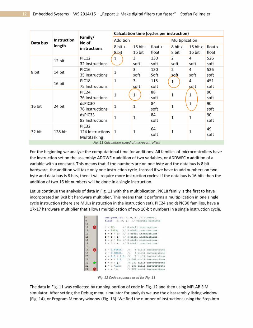
12 Embedded Systems – WS 2014/15 – „Report 1: Make digital filters run faster“ – Stefan Feilmeier
Fig. 11 Calculation speed of microcontrollers
For the beginning we analyze the computational time for additions. All families of microcontrollers have
the instruction set on the assembly: ADDWF = addition of two variables, or ADDWFC = addition of a
variable with a constant. This means that if the numbers are on one byte and the data bus is 8 bit
hardware, the addition will take only one instruction cycle. Instead if we have to add numbers on two
byte and data bus is 8 bits, then it will require more instruction cycles. If the data bus is 16 bits then the
addition of two 16 bit numbers will be done in a single instruction.
Let us continue the analysis of data in Fig. 11 with the multiplication. PIC18 family is the first to have
incorporated an 8x8 bit hardware multiplier. This means that it performs a multiplication in one single
cycle instruction (there are MULs instruction in the instruction set). PIC24 and dsPIC30 families, have a
17x17 hardware multiplier that allows multiplication of two 16-bit numbers in a single instruction cycle.
Fig. 12 Code sequence used for Fig. 11
The data in Fig. 11 was collected by running portion of code in Fig. 12 and then using MPLAB SIM
simulator. After setting the Debug menu simulator for analysis we use the disassembly listing window
(Fig. 14), or Program Memory window (Fig. 13). We find the number of instructions using the Step Into
Data bus Instruction length
Family/ No of instructions
Calculation time (cycles per instruction)
Addition Multiplication
8 bit + 8 bit
16 bit + 16 bit
float + float
8 bit x 8 bit
16 bit x 16 bit
float x float
8 bit
12 bit PIC12 32 Instructions
1 3 soft
130 soft
2 soft
4 soft
526 soft
14 bit PIC16 35 Instructions
1 3 soft
130 Soft
2 soft
4 soft
526 soft
16 bit PIC18 75 Instructions
1 3 soft
115 soft
1 4 soft
451 soft
16 bit 24 bit
PIC24 76 Instructions
1 1 88 soft
1 1 90 soft
dsPIC30 76 Instructions
1 1 84 soft
1 1 90
soft
dsPIC33 83 Instructions
1 1 84 soft
1 1 90 soft
32 bit 128 bit PIC32 124 Instructions Multitasking
1 1 64 soft
1 1 49 soft
13 Embedded Systems – WS 2014/15 – „Report 1: Make digital filters run faster“ – Stefan Feilmeier
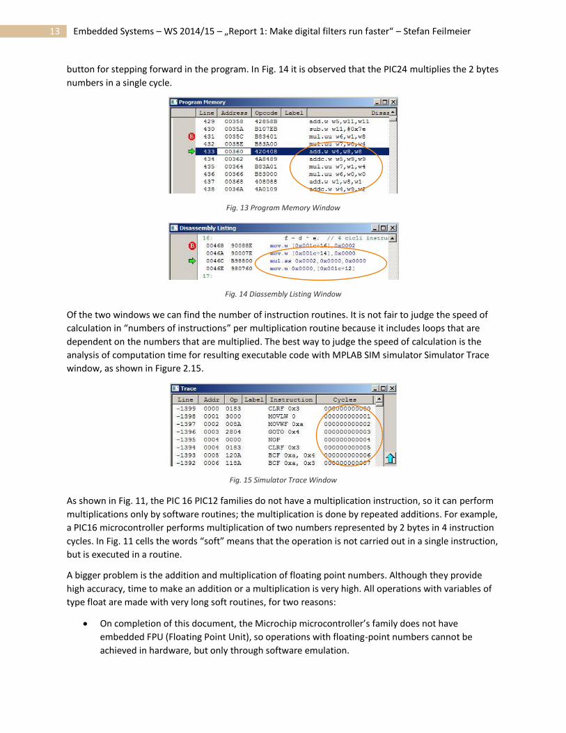
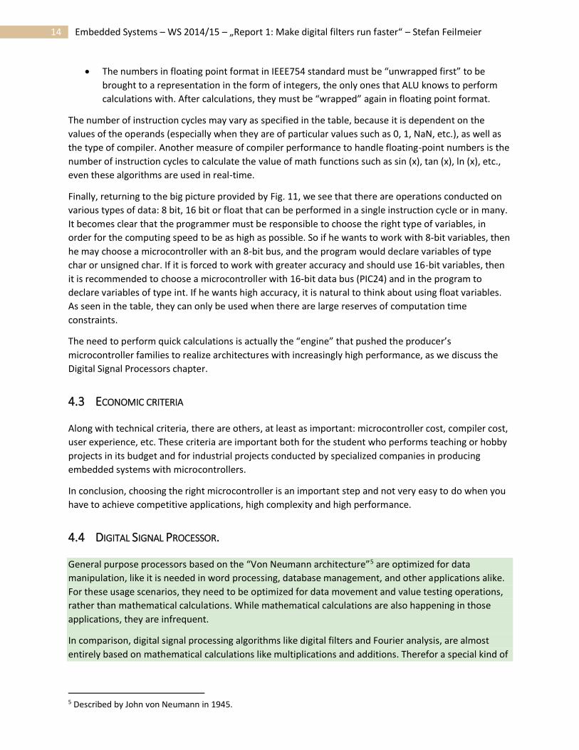
button for stepping forward in the program. In Fig. 14 it is observed that the PIC24 multiplies the 2 bytes
numbers in a single cycle.
Fig. 13 Program Memory Window
Fig. 14 Diassembly Listing Window
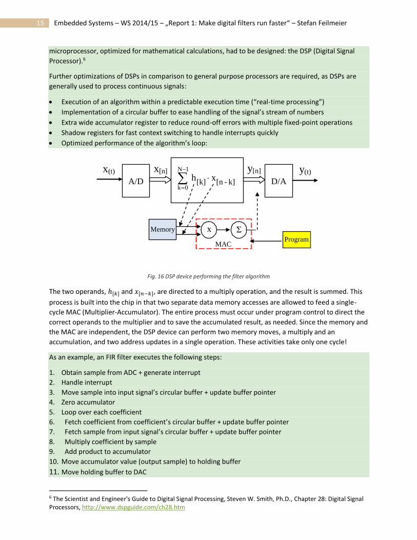
Of the two windows we can find the number of instruction routines. It is not fair to judge the speed of
calculation in “numbers of instructions” per multiplication routine because it includes loops that are
dependent on the numbers that are multiplied. The best way to judge the speed of calculation is the
analysis of computation time for resulting executable code with MPLAB SIM simulator Simulator Trace
window, as shown in Figure 2.15.
Fig. 15 Simulator Trace Window
As shown in Fig. 11, the PIC 16 PIC12 families do not have a multiplication instruction, so it can perform
multiplications only by software routines; the multiplication is done by repeated additions. For example,
a PIC16 microcontroller performs multiplication of two numbers represented by 2 bytes in 4 instruction
cycles. In Fig. 11 cells the words “soft” means that the operation is not carried out in a single instruction,
but is executed in a routine.
A bigger problem is the addition and multiplication of floating point numbers. Although they provide
high accuracy, time to make an addition or a multiplication is very high. All operations with variables of
type float are made with very long soft routines, for two reasons:
On completion of this document, the Microchip microcontroller’s family does not have
embedded FPU (Floating Point Unit), so operations with floating-point numbers cannot be
achieved in hardware, but only through software emulation.
14 Embedded Systems – WS 2014/15 – „Report 1: Make digital filters run faster“ – Stefan Feilmeier
The numbers in floating point format in IEEE754 standard must be “unwrapped first” to be
brought to a representation in the form of integers, the only ones that ALU knows to perform
calculations with. After calculations, they must be “wrapped” again in floating point format.
The number of instruction cycles may vary as specified in the table, because it is dependent on the
values of the operands (especially when they are of particular values such as 0, 1, NaN, etc.), as well as
the type of compiler. Another measure of compiler performance to handle floating-point numbers is the
number of instruction cycles to calculate the value of math functions such as sin (x), tan (x), ln (x), etc.,
even these algorithms are used in real-time.
Finally, returning to the big picture provided by Fig. 11, we see that there are operations conducted on
various types of data: 8 bit, 16 bit or float that can be performed in a single instruction cycle or in many.
It becomes clear that the programmer must be responsible to choose the right type of variables, in
order for the computing speed to be as high as possible. So if he wants to work with 8-bit variables, then
he may choose a microcontroller with an 8-bit bus, and the program would declare variables of type
char or unsigned char. If it is forced to work with greater accuracy and should use 16-bit variables, then
it is recommended to choose a microcontroller with 16-bit data bus (PIC24) and in the program to
declare variables of type int. If he wants high accuracy, it is natural to think about using float variables.
As seen in the table, they can only be used when there are large reserves of computation time
constraints.
The need to perform quick calculations is actually the “engine” that pushed the producer’s
microcontroller families to realize architectures with increasingly high performance, as we discuss the
Digital Signal Processors chapter.
4.3 ECONOMIC CRITERIA
Along with technical criteria, there are others, at least as important: microcontroller cost, compiler cost,
user experience, etc. These criteria are important both for the student who performs teaching or hobby
projects in its budget and for industrial projects conducted by specialized companies in producing
embedded systems with microcontrollers.
In conclusion, choosing the right microcontroller is an important step and not very easy to do when you
have to achieve competitive applications, high complexity and high performance.
4.4 DIGITAL SIGNAL PROCESSOR.
General purpose processors based on the “Von Neumann architecture”5 are optimized for data
manipulation, like it is needed in word processing, database management, and other applications alike.
For these usage scenarios, they need to be optimized for data movement and value testing operations,
rather than mathematical calculations. While mathematical calculations are also happening in those
applications, they are infrequent.
In comparison, digital signal processing algorithms like digital filters and Fourier analysis, are almost
entirely based on mathematical calculations like multiplications and additions. Therefor a special kind of
5 Described by John von Neumann in 1945.
15 Embedded Systems – WS 2014/15 – „Report 1: Make digital filters run faster“ – Stefan Feilmeier
microprocessor, optimized for mathematical calculations, had to be designed: the DSP (Digital Signal
Processor).6
Further optimizations of DSPs in comparison to general purpose processors are required, as DSPs are
generally used to process continuous signals:
Execution of an algorithm within a predictable execution time (“real-time processing”)
Implementation of a circular buffer to ease handling of the signal’s stream of numbers
Extra wide accumulator register to reduce round-off errors with multiple fixed-point operations
Shadow registers for fast context switching to handle interrupts quickly
Optimized performance of the algorithm’s loop:
x[n] y[n] x h
1N
0kk] -[n [k]
A/D
x(t) y(t)
D/A
Memory x Σ Program
MAC
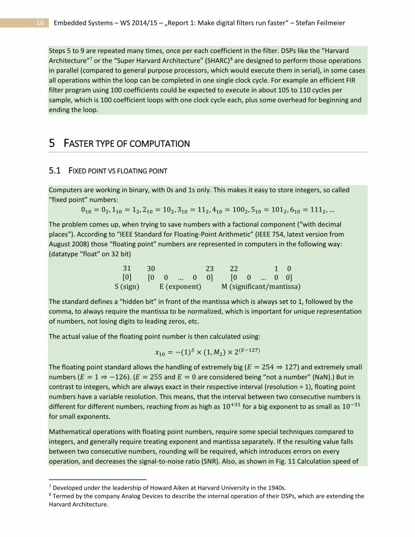
Fig. 16 DSP device performing the filter algorithm
The two operands, ℎ[𝑘] and 𝑥[𝑛−𝑘], are directed to a multiply operation, and the result is summed. This
process is built into the chip in that two separate data memory accesses are allowed to feed a single-
cycle MAC (Multiplier-Accumulator). The entire process must occur under program control to direct the
correct operands to the multiplier and to save the accumulated result, as needed. Since the memory and
the MAC are independent, the DSP device can perform two memory moves, a multiply and an
accumulation, and two address updates in a single operation. These activities take only one cycle!
As an example, an FIR filter executes the following steps:
1. Obtain sample from ADC + generate interrupt
2. Handle interrupt
3. Move sample into input signal’s circular buffer + update buffer pointer
4. Zero accumulator
5. Loop over each coefficient
6. Fetch coefficient from coefficient’s circular buffer + update buffer pointer
7. Fetch sample from input signal’s circular buffer + update buffer pointer
8. Multiply coefficient by sample
9. Add product to accumulator
10. Move accumulator value (output sample) to holding buffer
11. Move holding buffer to DAC
6 The Scientist and Engineer's Guide to Digital Signal Processing, Steven W. Smith, Ph.D., Chapter 28: Digital Signal Processors, http://www.dspguide.com/ch28.htm
16 Embedded Systems – WS 2014/15 – „Report 1: Make digital filters run faster“ – Stefan Feilmeier
Steps 5 to 9 are repeated many times, once per each coefficient in the filter. DSPs like the “Harvard
Architecture”7 or the “Super Harvard Architecture” (SHARC)8 are designed to perform those operations
in parallel (compared to general purpose processors, which would execute them in serial), in some cases
all operations within the loop can be completed in one single clock cycle. For example an efficient FIR
filter program using 100 coefficients could be expected to execute in about 105 to 110 cycles per
sample, which is 100 coefficient loops with one clock cycle each, plus some overhead for beginning and
ending the loop.
5 FASTER TYPE OF COMPUTATION
5.1 FIXED POINT VS FLOATING POINT
Computers are working in binary, with 0s and 1s only. This makes it easy to store integers, so called
“fixed point” numbers:
010 = 02, 110 = 12, 210 = 102 , 310 = 112 , 410 = 1002, 510 = 1012, 610 = 1112 , …
The problem comes up, when trying to save numbers with a factional component (“with decimal
places”). According to “IEEE Standard for Floating-Point Arithmetic” (IEEE 754, latest version from
August 2008) those “floating point” numbers are represented in computers in the following way:
(datatype “float” on 32 bit)
31[0]
30 23[0 0 … 0 0]
22 1 0[0 0 … 0 0]
S (sign) E (exponent) M (significant/mantissa)
The standard defines a “hidden bit” in front of the mantissa which is always set to 1, followed by the
comma, to always require the mantissa to be normalized, which is important for unique representation
of numbers, not losing digits to leading zeros, etc.
The actual value of the floating point number is then calculated using:
𝑥10 = −(1)𝑆 × (1, 𝑀2) × 2(𝐸−127)
The floating point standard allows the handling of extremely big (𝐸 = 254 ⇒ 127) and extremely small
numbers (𝐸 = 1 ⇒ −126). (𝐸 = 255 and 𝐸 = 0 are considered being “not a number” (NaN).) But in
contrast to integers, which are always exact in their respective interval (resolution = 1), floating point
numbers have a variable resolution. This means, that the interval between two consecutive numbers is
different for different numbers, reaching from as high as 10+31 for a big exponent to as small as 10−31
for small exponents.
Mathematical operations with floating point numbers, require some special techniques compared to
integers, and generally require treating exponent and mantissa separately. If the resulting value falls
between two consecutive numbers, rounding will be required, which introduces errors on every
operation, and decreases the signal-to-noise ratio (SNR). Also, as shown in Fig. 11 Calculation speed of
7 Developed under the leadership of Howard Aiken at Harvard University in the 1940s. 8 Termed by the company Analog Devices to describe the internal operation of their DSPs, which are extending the Harvard Architecture.
17 Embedded Systems – WS 2014/15 – „Report 1: Make digital filters run faster“ – Stefan Feilmeier
microcontrollers, these calculations have to be executed in software, if using a general purpose
processor without FPU (Floating-Point Unit), which is adding an enormous overhead. This overhead (and
many problems that are arising with the usage of fixed-point arithmetic) can be avoided using a
specialized Digital Signal Processor as introduced in chapter 4.4.
To make digital filters run faster on processors without Floating-Point Unit, it is recommended to use
fixed-point arithmetic, which can be calculated by a simple ALU (Arithmetic Logic Unit), instead of
floating-point. In Matlab this can be achieved using the following command:
Hf = fdesign.lowpass(0.4,0.5,0.5,80);
Hd = design(Hf,'equiripple');
Hd.Arithmetic = 'fixed';
Using this command, Matlab quantizes all filter into a fixed-point representation, which is per default set
to a wordlength of 16 bits, but can be adjusted to meet the required noise ratio.9 From then on, all
calculations in Matlab are fulfilled using fixed-point arithmetic, adjusting and increasing the bit-size of its
internal variables automatically.
6 PROGRAMMING TECHNIQUES
6.1 LOOK UP TABLE (LUT)
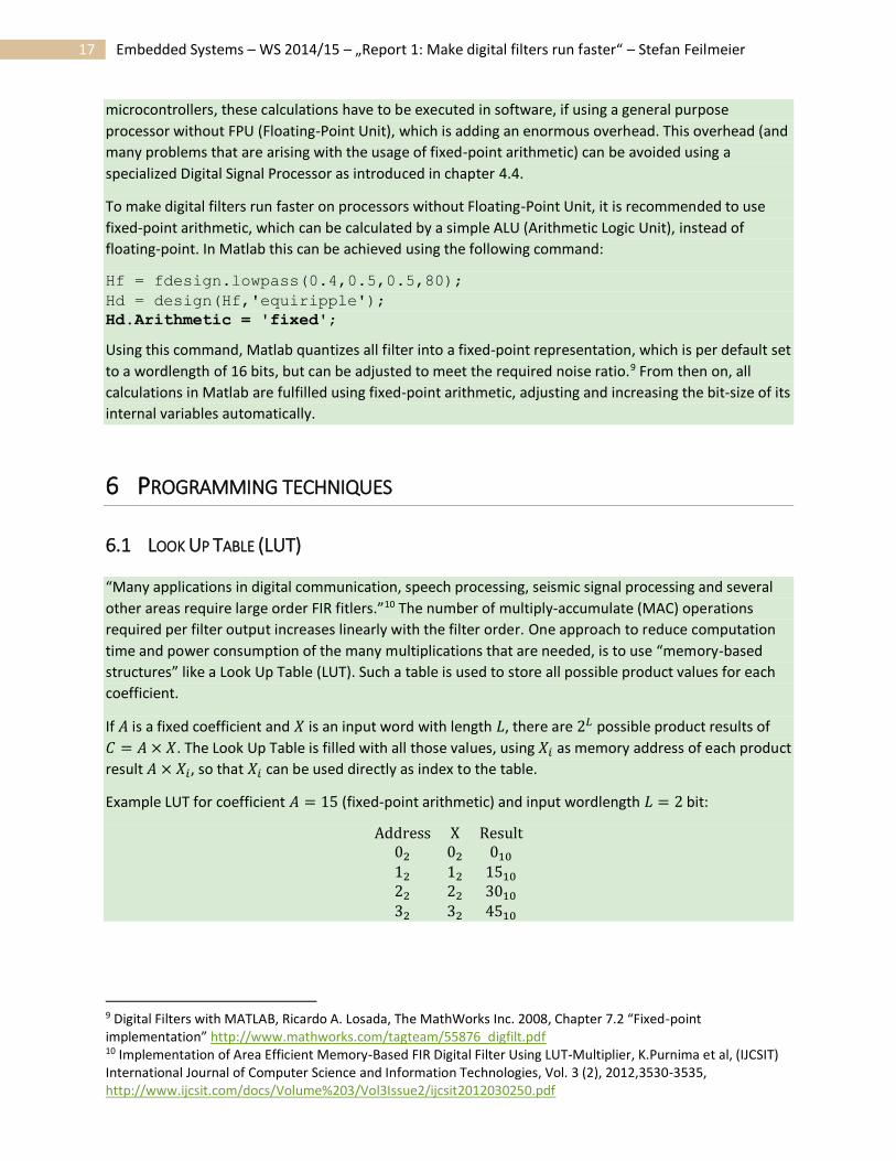
“Many applications in digital communication, speech processing, seismic signal processing and several
other areas require large order FIR fitlers.”10 The number of multiply-accumulate (MAC) operations
required per filter output increases linearly with the filter order. One approach to reduce computation
time and power consumption of the many multiplications that are needed, is to use “memory-based
structures” like a Look Up Table (LUT). Such a table is used to store all possible product values for each
coefficient.
If 𝐴 is a fixed coefficient and 𝑋 is an input word with length 𝐿, there are 2𝐿 possible product results of
𝐶 = 𝐴 × 𝑋. The Look Up Table is filled with all those values, using 𝑋𝑖 as memory address of each product
result 𝐴 × 𝑋𝑖, so that 𝑋𝑖 can be used directly as index to the table.
Example LUT for coefficient 𝐴 = 15 (fixed-point arithmetic) and input wordlength 𝐿 = 2 bit:
Address X Result02 02 010
12 12 1510
22 22 3010
32 32 4510
9 Digital Filters with MATLAB, Ricardo A. Losada, The MathWorks Inc. 2008, Chapter 7.2 “Fixed-point implementation” http://www.mathworks.com/tagteam/55876_digfilt.pdf 10 Implementation of Area Efficient Memory-Based FIR Digital Filter Using LUT-Multiplier, K.Purnima et al, (IJCSIT) International Journal of Computer Science and Information Technologies, Vol. 3 (2), 2012,3530-3535, http://www.ijcsit.com/docs/Volume%203/Vol3Issue2/ijcsit2012030250.pdf
18 Embedded Systems – WS 2014/15 – „Report 1: Make digital filters run faster“ – Stefan Feilmeier
6.2 PROGRAMMING LANGUAGE
Digital Signal Processing is nowadays not anymore only used in specialized DSP devices, but is used in all
kinds of systems and system environments. As an example, most of today’s mobile phones are running a
Linux-kernel based Android operating system. An Android frontend developer usually uses Java for his
applications, while the Linux-kernel is written mostly in C language with some parts in Assembly. Also
other compiled and interpreted programming languages like C++, Python, etc. are available in this
environment.
A programmer will for various reasons prefer to use the same programming language for each part of
his application. The question is: does it make sense to write the complete DSP processing in Java? Or in C
or Assembly?
There is no absolute answer to this question, as it highly depends on the specific system and economic
constraints. As a rule-of-thumb it can be expected, that a subroutine that is written “in Assembly will be
between 1.3 and 3.0 times faster than the comparable high-level program”11 in C. So depending on the
constraints it can or cannot be worth implementing some parts of the application in Assembly or, if they
exist, consider using libraries that provide algorithms implemented in Assembly.
In general, not limited to DSP, it is always an appropriate idea to implement everything in the preferred
and best fitting language for the environment and afterwards do a detailed profiling to find the
bottlenecks. Those subroutines should then be considered to be optimized or rewritten in a lower-level
language.
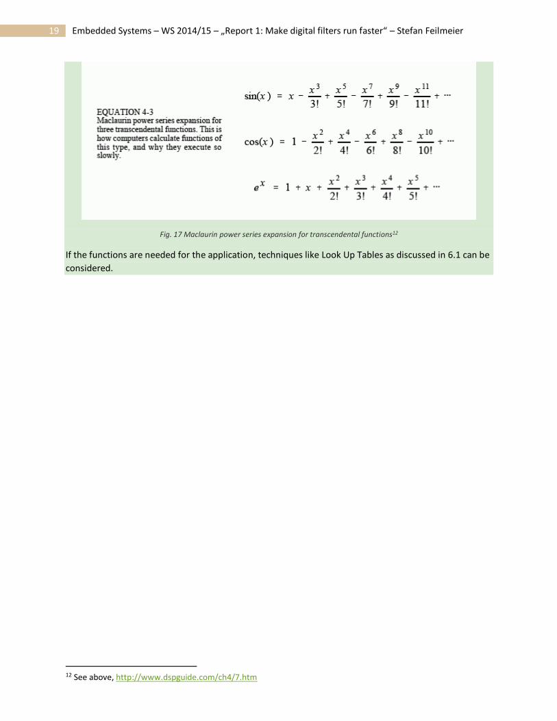
6.3 AVOIDING SLOW FUNCTIONS
As shown in 5.1 Fixed point vs floating point as well as in Fig. 11 Calculation speed of microcontrollers,
floating-point operations require a lot of computing time compared to fixed-point (integer) arithmetic.
Similarly, transcendental functions require huge calculation time when used in an algorithm. Therefor it
is necessary to know about them and to try to avoid or replace them if possible.
Examples for transcendental functions are:
sin(𝑥), cos(𝑥) , 𝑒𝑥 , 𝑥𝜋 , log𝑐 𝑥 for 𝑐 ≠ 0,1
11 The Scientist and Engineer's Guide to Digital Signal Processing, Steven W. Smith, Ph.D., Chapter 4: DSP Software, http://www.dspguide.com/ch4/5.htm
19 Embedded Systems – WS 2014/15 – „Report 1: Make digital filters run faster“ – Stefan Feilmeier
Fig. 17 Maclaurin power series expansion for transcendental functions12
If the functions are needed for the application, techniques like Look Up Tables as discussed in 6.1 can be
considered.
12 See above, http://www.dspguide.com/ch4/7.htm
20 Embedded Systems – WS 2014/15 – „Report 1: Make digital filters run faster“ – Stefan Feilmeier
TABLE OF FIGURES
Fig. 1 Digital filter 3
Fig. 2 Example of decimation 5
Fig. 3 Interpolation 6
Fig. 4 FIR filter (order 3) implemented in direct-form 7
Fig. 5 FIR filter (order 3) implemented in symmetric direct-form 8
Fig. 6 FIR filter (order 3) implemented in transposed direct-form 8
Fig. 7 IIR filter (order 3) implemented in direct-form 9
Fig. 8 Software tool for choosing appropriate μC 10
Fig. 9 Overview of Microchip μC families 10
Fig. 10 Summary of PIC families performances 11
Fig. 11 Calculation speed of microcontrollers 12
Fig. 12 Code sequence used for Fig. 11 12
Fig. 13 Program Memory Window 13
Fig. 14 Diassembly Listing Window 13
Fig. 15 Simulator Trace Window 13
Fig. 16 DSP device performing the filter algorithm 15
Fig. 17 Maclaurin power series expansion for transcendental functions 19
TABLE OF EQUATIONS
Eq. 1 Non-recursive filters 3
Eq. 2 Recursive filters 3
Eq. 3 Discrete Fourier Transform 3
Eq. 4 Fast Fourier Transform 4
Eq. 5 Cosine Transform 4
Eq. 6 FIR filter (order 3) implemented in direct-form 7
Eq. 7 FIR filter (order 3) implemented in symmetric direct-form 8
Eq. 8 FIR filter (order 3) implemented in transposed direct-form 8