Reporting versus Reputation:

Physician Quality and the Flexner Report of 1910

Brendon Patrick Andrews

(Northwestern University)

Job Market Paper

Draft Version: 13 November 2021

This paper is updated routinely.

For the most recent version: Click Here

Abstract: If patients can be persuaded to switch between licensed providers on the basis of au-thoritative opinions, policy-makers can harness such reporting as an additional tool to implementincentives for high-quality care. I employ the landmark Flexner Report (1910) medical schoolevaluations to show that reputations are a primary threat to effective reporting. This historic re-port did not target specific physicians, but ruthlessly disparaged the quality of American medicalschools and recommended the vast majority be closed. I show that doctors who recently entered alocal geographic market and who attended poorly-reviewed schools – not just the recent graduatesthereof – were about three times more likely to experience practice failure after the report’s release.Heightened practice failure implies that perceived quality and expected demand fell by enough tocompel market exit. I therefore capture monumental shifts in the viability of recent entrants’ physi-cian practices immediately after the release of weak negative signals. Expert recommendations haveconsiderably less impact when providers have established themselves in a market – no impact onpractice failure can be detected. These heterogeneous effects imply that policy-makers are unlikelyto dramatically alter consumer demand with quality information when trust and reputation areimportant market features – a strategy which targets existing relationships may be more powerful.

JEL Codes: D83, I11, J44, N31Keywords: Physician, Reputation, Quality Reporting, Certification, Flexner Report

Acknowledgements: Parts of this paper were developed as PhD coursework for Professors Joel Mokyr and JoeFerrie at Northwestern University, each of whom serves on my dissertation committee and whose expertise I bothgreatly admire and appreciate. Prof. David Dranove, who also serves on my committee, is owed an intellectual debtfor first suggesting I study the Flexner Report for my course requirements in Economic History. Innumerable helpfulsuggestions have been made by seminar participants at Northwestern, as well as at an early related presentation at theCanadian Economics Association in Banff, Alberta. All remaining errors are my own. I thank library staff at severallocations for their generous help and support viewing and/or documenting archival material related to this study.My doctoral studies at Northwestern were supported by a Northwestern University Fellowship and by Social Sciencesand Humanities Research Council of Canada Doctoral Fellowship No. 752-2016-0273. I gratefully acknowledge datagrants from the Center for Economic History and the Center for Applied Microeconomics at Northwestern, as well asa Graduate Research Grant from The Graduate School at Northwestern and an Exploratory Travel and Data Grantfrom the Economic History Association. Prof. Dranove also provided funding for external photocopies out of hisresearch account. All of these funds are currently being used to expand the scope of this project.

BrendonAndrews@u.northwestern.edu

copyright © Brendon Andrews 2021

1 Introduction

According to Adam Smith in his Lectures on Jurisprudence (1766), “A physician’s character is

injured when we endeavour to perswade [sic] the world he kills his patients instead of curing them,

for by such a report he loses his business” (Smith 1978, p. 399).1 The perspective that provider

demand can be affected by novel consumer information has generated many reporting initiatives.

For example, a consumer searching for hospital care in California now has access to the online

resources CMS Hospital Compare and Cal Hospital Compare. They might also consult the US News

and World Report hospital rankings. When seeking primary care, they could consult California’s

Office of the Patient Advocate report cards for medical groups.2 Before making an appointment with

a new doctor, a patient can also access an array of evaluations available through Yelp, Healthgrades,

ZocDoc, RateMDs, and other online platforms. Despite the widespread availability of information,

physicians designated as low-quality remain in business.3 In this paper, I use arguably the most well-

known and important quality evaluations in medical history – those contained in the Flexner Report

(Flexner 1910) – to show that otherwise successful interventions fail due to consumer learning,

trust, and established provider reputations. To move consumers away from low-quality physicians,

an alternative strategy which targets existing relationships may be necessary.

Written by Abraham Flexner and published by the Carnegie Foundation for the Advancement

of Teaching on 5 June 1910, the now-eponymous report entitled Medical Education in the United

States and Canada advocated major reform and assessed each medical school in these countries.

Some institutions received glowing appraisals while others were ruthlessly disparaged, and Flexner

stated that the vast majority of the region’s programs should be shuttered for quality concerns.

He did not introduce new ideas: his ‘muckraking’ pronouncements instead alerted the public to

information previously restricted to a medical audience (Ludmerer 2010) and helped shape pub-

lic opinion (Hudson 1992, p. 18).4 While the report evaluated institutions, graduates of poorly-

reviewed schools were routinely implicated in front-page news around the country. For example,

the Arkansas Gazette declared to its readers “Too Many Ill-Trained Doctors” (Arkansas Gazette 6

June 1910, p. 1) and the San Francisco Examiner exclaimed “Three-Quarters of Doctors ‘Quacks’”

(San Francisco Examiner 6 June 1910, p. 1).5 Consumers were suddenly warned about the quality

1Adam Smith’s contributions to early health economics were pointed out by Gaynor (1994).2Accessed 21 August 2021: https://www.opa.ca.gov/reportcards/Pages/default.aspx3Evidence that quality information affects provider demand is mixed. Some studies find no impact of reporting on

the quality of Coronary Artery Bypass Graft [CABG] surgeries on hospital volume or market share (Jha & Epstein2006, Wang et al. 2011). Yoon (2020) find that even though high-risk patients shift demand to low-mortality hospitalsafter CABG reporting, they are matched to low-quality surgeons at the selected hospital. Within hospitals, there issometimes considerable patient sorting across physicians by quality. Among rated surgeons in PA, Wang et al. (2011)find that quarterly CABG operations decrease by about 31.5% [an estimated decrease of 7.9 operations from a meanof 25.1] for high-mortality surgeons. Cutler et al. (2004) find that hospitals reported as high CABG mortality loseabout 10% of their related volume in the subsequent 12 month period, but this effect dissipates over time. Pope (2009)finds that hospitals improving their US News and World Report ranking by one spot are rewarded with 0.88% and1.06% increases in patient volume and associated revenue, respectively. The effect of quality reporting on consumerdemand ranges from null to dramatic.

4See Section 2.1 for details on previously circulating quality information in the medical community.5See Section 2.2 for more examples.

1

of their local physicians’ medical training. These easily understandable but indirectly targeted

evaluations constitute weak signals of physician quality, and patients could interpret his closure

recommendations as a form of third-party certification.

I show that doctors who recently entered a local geographic market and who attended poorly-

reviewed schools – not just the recent graduates thereof – were about three times more likely

to experience practice failure after the report’s release.6 Heightened practice failure implies that

perceived quality and expected demand fell by enough to compel market exit. I therefore capture

monumental shifts in the viability of recent entrants’ physician practices immediately after the

release of weak negative signals. Expert recommendations have considerably less impact when

providers have established themselves in a market – no impact on practice failure can be detected.

To establish these facts, I collected a novel dataset of annual physician practice locations and

educational details preserved in the Medical Directory of New York, New Jersey and Connecticut

(1903-1914). These directories are almost unique in the time period for their granularity; competing

national directories were published every 2-3 years.7 Consequently, the dataset permits the analysis

of physician practice failure by date of entry to a local market, which was previously untenable for

this era, and provides annual market duration data with specific years of exit. I digitized 120,989

physician-year records for 1903-1914 and manually linked these doctors across time and geography,

obtaining 14,261 unique individuals.8

Restricting attention to physicians practicing in the state of New York, I estimate duration

models of time to practice failure.9 Duration models estimate the effect of covariates x on a hazard

function λ(z, x) which gives the failure rate in period z for individuals with characteristics x,

conditional on having survived to the previous period. As a baseline, I employ the Cox (1972)

proportional hazards model, which sets λ(z, x) = ex′βλ0(z), where λ0(z) is a baseline hazard rate.

In discrete time, the Cox set-up is equivalent to a series of logistic models where the universe selects

which physicians fail in period z. Using a difference-in-differences specification of x′β, I show that

Flexner’s recommendations affected only physicians who entered a local geographic market within

the previous two years. Adding additional differences for recent graduation from poorly-reviewed

medical schools, I find that reporting affects all recent entrants and not only the less experienced

doctors for whom the information should be more relevant.

I differ from the literature in significant ways. Economic studies focused on modern healthcare

quality reporting initiatives directly estimate their impact on consumer choice of providers (Dranove

& Sfekas 2008, Pope 2009, Wang et al. 2011, Yoon 2020). This will not be possible. Microdata

6These effects are limited primarily to areas with sufficient differentiated competition – physicians with differentdegrees – and access to information shocks through a weekly general-content newspaper.

7Polk’s Medical Register and Directory of North America (1898-1917) was published in even years over the sampleperiod and the first four editions of the American Medical Directory (AMA 1907-1922) were published in 1906,1909, 1912, and 1914. California also produced statewide annual directories for 1903-1914 which are currently beingdigitized for an extension to this project.

8Data for Brooklyn and New York City were not digitized as the hypothesized ‘treated’ area for this project includesonly areas without a local medical school. See Section 3 for a detailed explanation of this important exclusion.

9Data for Connecticut and New Jersey appear to be imprecisely entered in the original documents. Market entrydates and survival times appear to be unreliable. See Section 3.

2

on physician-patient interactions from this time period do not broadly exist. I therefore cannot

identify small variations in consumer demand caused by the Flexner Report – my indirect approach

captures only reductions in a physician’s expected demand large enough to compel market exit. The

report’s recommendations may have impacted consumer demand for more established physicians,

but recent entrants were far more likely to be seriously affected. A major contribution of this

paper is to demonstrate that well-designed quality reporting can affect the viability of healthcare

providers by enough to compel market exit.10

Analyzing the Flexner Report also provides novel empirical evidence on the specificity of quality

information. Previous work has shown that even after controlling for available detailed measures,

consumers sometimes respond to coarse quality indicators (Spranca et al. 2000, Houde 2018, Bara-

hona et al. 2021). Coarse measures may help summarize complex information for inattentive con-

sumers. Flexner’s degree-based recommendations are coarse at the institutional level. The ratings

are even less precise at the level of individual practicing physicians and yet consumers respond to

these weak signals. This suggests that group-based or indirect ratings may be effective for some

consumers, possibly even when more detailed data are available.11

While I demonstrate that weak signals can be extraordinarily influential on the viability of

some doctors, the estimated impact on practice failure disappears when consumers are familiar

with a physician. This highlights the importance of market learning & news (Dafny & Dranove

2008, Dranove & Sfekas 2008) as well as established reputations (Xiao 2010) in tempering the

effect of quality information. Trust is a primary feature of healthcare markets (Arrow 1963), and

so reputation may be particularly relevant for regulators designing quality reports for individual

practitioners. As consumers ignore otherwise powerful expert recommendations when they have

established relationships with providers, policymakers may find it difficult to shift market outcomes

dramatically through information alone. An alternative strategy which targets existing relationships

may be more effective, but which policy maximizes consumer welfare is left an open question.

The remainder of this paper is organized as follows. First, I discuss related literature. Next,

I provide the historical setting for the Flexner Report in Section 2, providing context for its rau-

cous reception. I also provide details on the specifics contained in the report and related quality

information available to the contemporary consumer. The medical directory data is described in

10Heightened practice failure has been documented for Coronary Artery Bypass Graft [CABG] surgeons revealed ashigh-mortality options, but these results are tenuous due to minuscule sample sizes. Jha & Epstein (2006) investigatethe New York CABG reporting system using 168 surgeons rated between 1989 and 2002. They find that surgeons inthe bottom quartile of reported risk-adjusted mortality quit their New York CABG practice within 2 years at a rateof 20% as compared to 5% for the other practitioners (p. 849-850). Yoon (2020) produces statistics from a total of87 surgeons in New Jersey, of whom only 45 were rated. The present data structure and sample size permit both amore in-depth analysis of rated physicians’ practice failure, as well as greater statistical precision.

11This may be a fruitful area for future research. For example, in 2009 the United States Congress passed the ‘FamilySmoking Prevention and Tobacco Control and Federal Retirement Reform Act’ (H.R. 1256, 111th U. S. Congress2009), which required the Food and Drug Administration [FDA] to publicize a “list of harmful and potentially harmfulconstituents, including smoke constituents, to health in each tobacco product by brand and by quantity in each brandand subbrand” (section 904(e)). Consumers may respond to quality information published at the brand level evenwhen sub-brand level data are available, and how consumers use brand versus sub-brand quality information mayhave important welfare implications.

3

detail in Section 3, and restrictions are made to the analysis sample based on preliminary findings.

In Section 4, I relate physician practice failure to ‘hazards’ in duration models, and lay out my

approach to estimation. Section 5 provides my main results, assesses the impact of differentiated

competition and access to information, and shows that market readjustment was rapid. In my

concluding discussion, I search for evidence of sorting and gaming behavior ex-post, discuss general

equilibrium national trends, link my results to reputation and consumer demand, and conclude

with policy lessons for modern regulators and questions for health economists.

1.1 Related Literature

Reporting initiatives are one of many institutions which may develop to offer consumers quality

assurance in markets with quality uncertainty.12 In the absence of supplementary information,

low-quality providers can drive out high-quality providers, decreasing the overall size of the market

and degrading average quality (Akerlof 1970). When quality guarantees are non-formal, consumer

trust becomes central. This is especially true for the decision to seek medical care, as potentially

life-threatening illnesses and errors from untalented physicians make healthcare unique in its con-

sequential nature combined with its heightened uncertainty (Arrow 1963). It is not possible to

sample medical care, and so consumers must search for information on physician quality primarily

through direct experience (Nelson 1970) or through reputation channels such as recommendations

from friends or family (Satterthwaite 1979).

An influx of novel quality information can be modeled as a negative shock to a provider’s

reputation. In his basic model, Holmstrom (1999) shows that learning about managerial ability

depends on the amount of information available: early output observations are weighted heavily,

but eventually talent is fully revealed and new observations do not impact beliefs. The heightened

availability of information makes new signals less valuable, reducing the value of reporting for

established physicians, and the same intuition underpins the average model of recommendations

presented in Section 6.4. Board & Meyer-ter-Vehn (2013) model reputational learning as perfect

good news or bad news signals, and find the latter is characterized by shirk-work equilibria – when

reputation falls below some threshold, firms will shirk. Cabral & Hortacsu (2010) find that eBay

sellers who receive a negative review are more likely to receive additional negative reviews and are

subsequently more likely to exit. My results are consistent with a negative quality signal causing

recent entrants to shirk within a local market and subsequently exit.

As I do not observe physician-patient relationships, I cannot fully differentiate between repu-

tation, trust, established relationships, and other forms of market-based learning which entrench

patient demand for a physician’s services over time. Trust is a key feature of healthcare mar-

kets (Arrow 1963, Frank 2007) and may be particularly relevant for consumers with established

physician-patient relationships, who may use direct experience to evaluate uncertain product qual-

ity (Nelson 1970). A consumer with previous positive experiences may have developed trust in

12For hospitals, Dranove & Jin (2010) list brand-names, experience & word of mouth, industry-sponsored voluntarydisclosure, third-party disclosure, government-mandated disclosure, and licensing (p. 938).

4

their physician’s competence, and external reputations may have no impact on their decisions. To

the extent that established providers have more loyal customers, my results may actually reflect

the protective effect of direct relationships, not established reputations.

I contribute most directly to the literature concerned with quality reporting for medical providers.

A strong plurality of these studies focus on risk-adjusted mortality reporting for Coronary Artery

Bypass Graft [CABG] surgeries (Schneider & Epstein 1996, 1998, Burack et al. 1999, Cutler et al.

2004, Mukamel et al. 2004, Jha & Epstein 2006, Dranove & Sfekas 2008, Wang et al. 2011, Yoon

2020).13 Relationships between these specialists and patients are mediated by referring physicians,

complicating the link between physician-patient trust and practice failure, but high-mortality sur-

geons have been shown to be more likely to quit practice after the release of CABG surgery report

cards (Jha & Epstein 2006, Yoon 2020). My main results advance this narrative: effective quality

reports can actually be powerful enough to compel low-quality providers to exit markets.14

This paper also provides additional evidence on market learning and which features make re-

porting effective. Dafny & Dranove (2008) demonstrated that health plan consumers learn from

reporting, but market learning dominates. Dranove & Sfekas (2008) find that only hospitals re-

ceiving negative news in New York’s CABG program were impacted – a naive model which treats

all low-quality information the same finds no impact. My results are aligned with the observation

that reporting is effective when it facilitates learning. First, the Flexner Report had no impact

on the viability of physicians for whom local consumers had more than two years of market-based

learning opportunities. Second, I show that increases in practice failure are loaded on physicians

who attended institutions rated highly in lenient less-publicized reports, but disparaged by Flexner.

Previous research has shown that coarse measures of quality disclosure are consequential for

consumer decision-making ranging from health plans (Spranca et al. 2000) to energy efficiency in

refrigerators (Houde 2018) to sugar/calories in breakfast cereals (Barahona et al. 2021). Flexner’s

closure recommendations were coarse at the medical school level, and were even more imprecise

with respect to individual practitioners. These weak signals were enough to dramatically affect the

viability of recent entrants’ practices immediately after the release of the Flexner Report, suggesting

that many consumers are willing to use both indirectly targeted & coarse quality information.

Additional research will be required to determine how consumers combine indirectly targeted and

specific quality information when both are available.

Put another way, Flexner’s recommendations are a form of warning labels for licensed profes-

sional services, a potential policy option for regulators and third-party certifiers in lieu of more

aggressive licensing regimes. Friedman (1962) writes passionately against both certification and

licensing, but finds “it difficult to see any case for which licensure rather than certification can

13There are also papers which investigate the effect of reporting across differing specialties in other states such asCalifornia (Romano & Zhou 2004, Pope 2009) and Wisconsin (Hibbard et al. 2005).

14Other narratives are slowly emerging. Reporting has been documented to cause an increase in provider-patientsorting for both hospitals (Dranove et al. 2003, Cutler et al. 2004) and surgeons (Mukamel et al. 2004, Yoon 2020).This may be explained by provider gaming (Schneider & Epstein 1996, Burack et al. 1999) or capacity constraints(Yoon 2020). Reporting can also spur quality improvements (Cutler et al. 2004, Hibbard et al. 2005, Smith et al.2012, Vallance et al. 2018, Eyring 2020).

5

be justified” (p. 149). The results of the present study provide unique empirical evidence con-

cerning how consumers respond specifically to medical certification substituted for more aggressive

licensing in an era where gross variation in quality persisted. I find that policymakers may find it

difficult to shift market outcomes dramatically through certification or information alone when pa-

tients have established relationships with providers. I suggest an alternative strategy which targets

existing relationships, but which policy – certification, aggressive licensing, or targeting specific

physician-patient relationships – maximizes consumer welfare is left an open question.15

This paper also makes significant inroads in economic and medical history. While previous work

has shown that the Flexner Report impacted medical school survival (Hiatt & Stockton 2003, Miller

& Weiss 2008, 2012, Weiss & Miller 2010), this paper contributes both by modeling the Flexner

Report as a shock to consumer information and analyzing its impact on practicing physicians. My

results further advance our understanding of how early medical education reforms restructured

the availability and composition of American physicians.16 Moehling et al. (2020) found that as

medical education reform increased the quality of medical graduates, preferences for urban location

increased, widening the urban-rural gap in equilibrium physician supply.17 By tracking individual

physicians across time, I complement their approach by showing that relocating physicians typically

also selected larger urban locations. While differential ratings in the Flexner Report cannot explain

shifts in physician density, these results suggest that location preferences were shifting globally,

and not just among high-quality entrants.18 In addition, physicians relocating for at least a second

time move to less populated locations, a result which mirrors the pattern for failing physicians

some decades later in 1971-83 (Marder 1990). Life cycle patterns in physician practice locations

are therefore similar under very different institutional regimes, heightening our confidence that

physician behaviors may be fundamentally comparable over diverse settings.

2 Historical Setting

Evaluations of a physician’s undergraduate education may not appear to be a powerful quality

measure to the modern reader. The path to obtaining medical credentials in the United States

today is a long and arduous journey involving extensive training. To enter a medical school in

the United States, students are required to demonstrate extensive premedical training with specific

requirements.19 The four-year medical degree is now standard, with approximately 10% of matric-

15Policymakers may lack information available to consumers, leading to regulatory errors.16Moehling et al. (2019) find that medical education reform led to a large decrease in female physicians from a

peak around 1900. This occurred due to both the closure of women-only schools and substitution from female tomale students as the entry requirements increased and overall enrollment decreased. Owing to the small proportionof physicians educated in female-only medical schools in any given year, I cannot separately estimate the effect ofquality reporting in the Flexner Report on practicing female physicians.

17Their primary measure of quality was whether a school required entrants to have 1-2 years of college education.18It is possible that the influx of young high-quality entrants were the factor that made urban areas more attractive

to relocating physicians. I leave such questions to future research.19For example, Harvard Medical School requires a baccalaureate degree of at least three years with requirements

in biology, chemistry/biochemistry, physics, and writing. Premedical laboratory work is required and coursework inmathematics and behavioral sciences are encouraged. See ‘Prerequisite Courses’ on Harvard Medical School’s website:

6

ulates now graduating after five years (AAMC 2020b). Three regulated examinations are required

during training to obtain a medical license in the United States, with the final examination taking

place after prospective physicians have matched with a medical residency – post-graduate training

in which they’ll be engaged for 3-7 years depending on specialty, including general practitioners of

family medicine.20

The modern American physician seeing patients has thus typically engaged in at least 10 years

of post-secondary education involving three distinct components.21 The human capital investment

is convoluted and difficult to disentangle – the most promising students attend the best medical

schools and are matched with the most renowned residency programs. Medical degree quality may

not even be a pertinent source of information concerning the overall quality of training a physician

received: their residency was more recent, tailored to their specialization, and these programs

assessed the quality of applicants conditional on their undergraduate performance. Consequently,

modern evaluations of medical school training may not actually provide any useful information for

healthcare consumers.

The Flexner Report made an appreciable impact on public consciousness (Hudson 1992, Lud-

merer 2010) in a very different America. In the section which follows, I demonstrate that (i)

physicians in 1910 were primarily engaged in general practice; (ii) undergraduate medical educa-

tion represented the lion’s share of a practitioner’s training; (iii) gross variation persisted among

licensed physicians; (iv) physicians signaled quality using gameable aesthetic considerations; and (v)

Flexner’s evaluations of laboratory and clinical competence were particularly salient for healthcare

consumers in this era. In this context, the information in the report was a relatively clear heuristic

for prospective patients concerned about the expected quality of a potential physician. Section

2.2 describes the report, the informational setting in which it was released, and its widespread

dissemination.

2.1 Medical Training in 1910

When President William McKinley was shot in Buffalo in September 1901, the surgeon who oper-

ated on his wounds specialized in gynecology. His performance has led to suggestions of possible

malpractice or guilt in the President’s untimely death (Markel 2019), but this type of medical

arrangement was not uncommon.22 The dominance of specialists among physicians in the United

States had not yet been established, and those who did specialize also engaged in general practice.

By 1923, only about 9.2% of physicians in the AMD could be classified as full-time specialists.23

https://meded.hms.harvard.edu/admissions-prerequisite-courses. Accessed 2 August 2021.20See ‘Board Certification Requirements’ on the American Board of Medical Specialties website: https://www.

abms.org/board-certification/board-certification-requirements/. Accessed 2 August 2021.21Extensive clinical training, various clerkships, and internships are also typically completed, including by premed-

ical students.22As it happens, the gynecological surgeon was Matthew D. Mann, who appears in the dataset used in this paper.23There were 145,969 physicians in the 1923 edition of the AMD. There were 15,408 full-time specialists – excluding

interns and residents – of which 1,958 practiced internal medicine in 1923 (Stevens 1971, Table 1, p. 162). If wechoose to include internal medicine as general practitioners instead, the percentage becomes 10.6%. Stevens reportsthat internal medicine was considered the third largest specialty in 1923, while the largest segment was a glut of

7

Even by 1931, about 82.9% of practicing physicians – excluding interns, residents and fellows –

were general practitioners or engaged in part-time specialism (Stevens 1971, Table 2, p. 181). The

typical American physician was engaged in at least some general practice throughout the first three

decades of the twentieth century. Stevens showed this had already changed by 1969, when full-

time specialists accounted for 77.1% of physicians in the United States. In 2019, at most 12.6% of

American doctors list family medicine & general practice as their specialty (AAMC 2020a).24

As specialists were not yet omnipresent, medical residencies – the cornerstone of modern medical

education – were also less prevalent. In fact, the AMA did not publish a list of hospitals approved

for residencies until 1927. In this number, the AMA listed 1,699 educational residencies at 270

hospitals (AMA 1927, p. 829).25 These educational residences were distinct from salaried ‘resident’

physicians and were also referred to as ‘advanced’ or ‘special’ internships. An editorial to the

Journal of the American Medical Association [JAMA] in 1940 notes that there were only 428

special internships in 1914 (JAMA 1940) – residencies as we know them today were a complete

non-factor in 1910.

Special internships were a natural evolution of the existing hospital intern position occupied

by many recent medical graduates in the early twentieth century. This internship system arose

naturally in the United States, without the direction of medical schools, and so early statistics on

this training are sparse. John Rose Bradford, a professor of medicine at University College London

contrasted the role of hospital staff in relation to medical schools in the United States and Britain

in his report to the Mosely Education Commission in 1904. The disconnection of hospital training

from the standard medical training in the United States – with the exception of Johns Hopkins26

– was highlighted, but he noted that the American “interne” system had the benefit of using more

advanced graduates in hospitals, and these recruits could apply acquired knowledge and skill. He

was disheartened that only “about half the students in the leading medical schools” made use of

a hospital internship before practice (Mosely Education Commission 1904, p. 66). By 1913, some

66-70% of American medical graduates were partaking in a hospital internship27 but no American

medical school required it for graduation and neither did any state licensing board require it for

certification (Council on Medical Education and Hospitals 1960, p. 21).

The quality of the medical training of a contemporary physician was therefore determined

primarily by their medical degree. In addition, having obtained a medical degree was not necessarily

an indication that a doctor was well-qualified to practice medicine. Among medical schools from

4,703 ophthalmologists and otorhinolaryngologists. The second largest group the 3,336 surgeons & practitioners ofoccupational medicine.

24At most another 12.8% of the nation’s 938,980 practitioners specialize in internal medicine. Put together, thesetwo fields account for just barely over a quarter of American physicians belonging to a ‘specialty’ of at least doctors.Additional specialists may engage in part-time general practice.

25Council on Medical Education and Hospitals (1960) states that there were 278 hospitals with 1,776 such positionsin 1927 (p. 28). JAMA (1940) also refers to 1,776 residencies in 1927.

26The Canadian schools were also noted as exceptions in the North American context.27There were at least 3,006 interns in the United States and about 4,500 medical graduates annually (66.8%), and

reports from a subset of the medical schools indicated the rate was approximately 70% (AMA 1913, p. 2017). Thereason stated from the medical schools was that the remaining graduates did not wish to pursue an internship. Theissue was with intern supply, not demand from clinical providers.

8

whom at least 50 graduates presented before state examining boards, failure rates in 1904 ranged

from 0.6% for Harvard to 69.2% for Baltimore University (AMA 1905, p. 1455). State licensing

boards only weeded out the bottom of the barrel; incompetent physicians managed to pass the

examinations.28 Examinations for the Marine Hospital Service and the medical corps of the Navy

and Army were assessed to be more difficult and more practical than state board examinations,

and had correspondingly higher failure rates (Flexner 1910, p. 170). As most examinations were

written, purely didactic methods or what now we call “teaching to the test” could propel students

into practice.

Keen followers of medical statistics might have been able to parse some information regarding

the relative quality of medical schools through the reading of these state board statistics in JAMA.

This would not have represented the average patient. In 1910, about 62.6% of JAMA subscribers

were members of the AMA in 1910.29 Most of the remaining subscribers were probably physicians

not yet converted to membership in the AMA.30 As it stood, according to Abraham Flexner in the

famed report, the layperson couldn’t differentiate between graduates of Harvard and the Boston

College of Physicians and Surgeons, and usually didn’t even know their medical alma mater (Flexner

1910, p. 172).

Prior to the release of his findings, the public wasn’t very astute in evaluating the medical

profession. So detached from professional training was medical reputation that self-help manuals

were employed by the physician in improving their respectability among the local clientele. Among

the highly popular of these manuals for the recent medical graduate was D. W. Cathell’s The

Physician Himself and What He Should Add to the Strictly Scientific, first published in 1882 and

later renamed Book on the Physician Himself and Things that Concern His Reputation and Success

(King 1984, p. 102). The state of medical practice around the time of the Flexner Report can be

ascertained from a reading of the recommendations in the 1911 edition:31

Public opinion is the supreme court. You will be more esteemed by patients who call at

your office, for any purpose, if they find you engaged in your professional duties and studies,

than if playing music, making toy steam-boats, entertaining loungers, or occupied in other non-

professional or trivial pursuits; even reading the newspapers, smoking, etc., at times proper for

28There were many avenues, including successive reexamination, to achieve this end. As well, the typical passingrate was 75 percent overall, without a minimum standard by category. This meant that a physician could pass thetest and be grossly incompetent. For example, in June 1906, one unnamed physician from the Baltimore MedicalCollege [distinct from Baltimore University] passed the Maryland examinations with a score of 79 percent but only56 percent in anatomy. Another physician from the same college passed (75 percent) with 57 percent in pathologyand 49 percent in chemistry (AMA 1906).

29Circulation of the AMA in 1910 was 54,577 according to N. W. Ayer & Son’s American Newspaper Annual andDirectory (Ayer & Ayer 1910). Membership in the AMA reached 34,176 as of 1 May 1910 (AMA 1910a, p. 1963).Members of the AMA are assumed to be subscribers to JAMA because it was required for membership in the AMABy-Laws by 1909; see ‘Chapter I. – Qualifications for Membership’ in the 1909 edition of the American MedicalDirectory (p. 2).

30Based on 135,317 physicians listed in the in the United States in the 1909 edition of the AMD, it is likely thatover 100,000 physicians were non-members of the AMA. The remaining 20,401 average annual recipients of JAMAcould easily be physicians. Moreover, the AMA added 3,593 members between 1909 and 1910, of which 2,628 (73.1%)were previously non-member journal subscribers (AMA 1910a, p. 1963). Taken together, this is highly suggestivethat non-medical audiences were likely not reading JAMA in large numbers.

31This edition had been revised by his son William T. Cathell.

9

study and business, have an ill effect on public opinion, which is the creator, the source of all

reputation, whether good or bad, and should be respected; for a good reputation is a large, a

very large, yea one of the chief parts of a physician’s capital (Cathell & Cathell 1911, p. 11)

Specific recommendations also include to avoid making friends with ‘aimless idlers’, to grow a

beard if possessed of a ‘youthful-looking’ face, and not to shake hands with the coarse or ignorant.

Physicians should decorate their office with degrees, awards, society memberships, and photos of

medical celebrities or heroes. This was a manual aimed at the former working class, attempting to

cultivate an image in the professional world – the goal was to imply credibility.

Medicine had undergone an overall quality explosion in the preceding decades. Robert Koch’s

discovery and description of the ‘tubercle bacillus’ in The Etiology of Tuberculosis in April 1882

(Koch 1882) is widely regarded as the paradigm-shifting moment in the rise of germ theory.32

Understanding the causative agents of infection led to a revolution in healthcare. In the 1880s,

40% of abdominal and pelvic surgery patients died of complications; in 1900, the death rate was

5% (Stevens 1971, p. 49). Improvements in child mortality were so drastic that life expectancy

at birth improved by about 7.1 years among white Americans between 1880 and 1900 (Preston

& Haines 1991, p. 129).33 By the turn of the century, laboratory work took on an enlarged role

(King 1984), as a physician could harness scientific methods to accurately diagnose a lengthy list of

conditions including cholera, leukemia, infection with the parasitic worm filaria, malaria, leprosy,

amoebic dysentery, and diphtheria, among others (Musser 1898, p. 1490).

Progress meant that proper medical care was effective, aggravating the difference between ‘good’

and ‘bad’ medicine. The novel methods worked. It is therefore not shocking that Flexner (1910)

devoted a lot of ink to the praise of the German model of medical education, and the benefits

of strong clinical and laboratory training. The main criticisms of each school he disparaged are

typically found under categories entitled ‘laboratory facilities’ and ‘clinical facilities’. Prospective

patients now faced a choice that mattered in context: hire a physician with proper knowledge

of the literally life-saving state of the art, or risk life and limb by contracting the services of a

physician with lesser training. Given the gross variation in quality among physicians available, the

methods by which contemporary consumers assessed physician quality, and the narrow dimensions

of medical training, the public was seemingly susceptible to have their perceptions of physician

quality shocked by a well-designed report on the efficacy of medical training.

2.2 Flexner’s Shocking Report

The abysmal and highly variable training of physicians in the nineteenth century was noticed by

expert contemporaries. Since its inception in 1847, the American Medical Association [AMA] has

32A contemporary review of Koch’s work, published in July 1882 in the American Journal of the Medical Sciences,stated that Koch’s new staining procedure determined the cause of tuberculosis ‘beyond doubt’ (AJMS 1882).

33These improvements in mortality were estimated nationally using questions about children and surviving childrenfrom the 1900 federal census. Preston & Haines (1991) find no evidence of improvement for black Americans overthe same time period.

10

avowed improvements in medical education and public health as two of its primary goals (AMA

2021). Not much was done.34

Eventually, a new era of standardization in medical education was initiated in 1904, when the

AMA created its Council on Medical Education [CME]. The CME was entrusted with the review of

medical degree-granting institutions in the United States and Canada, with the set aim of enforcing

minimum standards for the education of physicians. To accomplish this goal, the CME began

inspecting institutions in 1906. The CME presented the results of its 1906 inspections at its Third

Annual Conference in Chicago on 29 April 1907 (AMA 1907). For each medical school, 0-10 points

were assigned to each of ten categories.35 A grade of A was assigned to medical schools scoring

90 or higher, B was assigned to 80-90, and C was assigned to scores of 70-80. All three categories

were considered acceptable. Grades of D and E were given to 60-70 and 50-60, respectively; these

schools needed some improvements. Scores below 50 were considered unacceptable and given a

score of F. Of the 160 American medical schools evaluated, 81 were assigned grades A-C, 47 needed

improvements, and 32 were assigned a failing grade of F. The list of schools receiving each grade

was not publicized, and only summary statistics were available in the Journal of the American

Medical Association.

The public and the profession have largely forgotten this and earlier initiatives, and remember

instead Flexner’s quality reporting in June 1910. His obituary in the New York Times was front-

page news, and its first sentence claimed his report “revolutionized medical studies in the United

States” (New York Times 22 Sept 1959, p. 1). This legacy has endured. When the New England

Journal of Medicine began a new series concerned with medical education, the introductory article

was entitled “American Medical Education 100 Years after the Flexner Report” (Cooke et al. 2006),

and in introducing a special centenary issue for the report in 2010, the editor of Academic Medicine

assumes readers will be celebrating the 200th anniversary in 2110 (Kanter 2010). Why? While

Flexner did not introduce new ideas to medical audiences, his ‘muckraking’ pronouncements were

novel for general audiences and helped shape public opinion (Hudson 1992, Ludmerer 2010).

Despite its impact, the methodology of the Flexner Report was not overwhelmingly transparent.

He provided brief details on each school’s history, entrance requirements, fees, attendance, teaching

staff, and other teaching resources. Emphasis was placed on laboratory facilities and clinical facil-

ities. In several places in the text, Flexner makes personal recommendations as to which schools

ought to remain in operation and which should be closed. Ultimately, he calls for a reduction

34This might have been due to the relatively dismal state of the profession previously. As the capabilities ofmedicine improved, so too did the power of the AMA. Membership in the AMA more than doubled between 1904and 1910. Listed at 15,039 as of 1 May 1904 (AMA 1904, p. 1575), it reached 34,176 as of 1 May 1910 (AMA 1910a,p. 1963).

35These categories were: (i) “showing of graduates before state board examinations;” (ii) “requirements and en-forcement of satisfactory preliminary education;” (iii) “character and extent of college curriculum;” (iv) “medicalschool buildings;” (v) “laboratory facilities and instructions;” (vi) “dispensary facilities and instruction;” (vii) “hos-pital facilities and instruction;” (viii) “extent to which first two years are officered by men devoting entire time toteaching and evidences of original research work;” (ix) “extent to which the school is conducted for the profit of thefaculty directly or indirectly rather than teaching;” and (x) “libraries, museums, charts, etc.” (AMA 1907, p. 1702).

11

from 147 to 31 schools in the United States.36,37 Three of the eight Canadian schools were to be

eliminated. When describing the quality of medical training at the schools he wanted closed, he

was often eviscerating: both Milwaukee schools were “without a redeeming feature,” (p. 319) and

he described the dissecting facilities at Chicago’s National Medical University as “a dirty, unused,

and almost inaccessible room containing a putrid corpse, several of the members of which had been

hacked off,” (p. 213). His apparent goal was to shock and awe the public consciousness.

It worked. The following morning, 6 June 1910, its publication was front-page news across the

country. The Chicago Tribune’s cover was emblazoned with “Scores Chicago’s Medical Schools:

Carnegie Foundation Says This City in That Line of Education Is Plague Spot of the Country”

(Chicago Daily Tribune 6 June 1910, p. 1). In Boston, the Herald’s front page alerted readers

“Carnegie Report Bitterly Assails Medical Schools” (Boston Herald 6 June 1910, p. 1). In Bal-

timore, The American reported a defensive attitude: “Deans Defend the Schools: Attacked By a

Carnegie Report” (Baltimore American 6 June 1910, p. 1). Across the country, the Omaha Morn-

ing World-Herald declared “Says Country Supports too Many Doctors: Abraham Flexner Scathes

Medical Schools in Report to Carnegie Foundation” (Morning World-Herald 6 June 1910, p. 1),

and in Little Rock, the Arkansas Gazette’s cover put the matter simply in bold face, “Too Many

Ill-Trained Doctors” (Arkansas Gazette 6 June 1910, p. 1).

36Flexner states this as 155 to 31 (p. 154). This conflicts slightly with the tabulation of recommendations I providebelow in Table 1. Flexner described 170 schools in the United States and Canada. Eight of these schools wereCanadian, leaving 162 American schools. It is unclear how Flexner arrives at 155 schools in the United States. Thisnumber likely refers to 170 schools less the 3 schools which closed prior to his report and the 12 post-graduate orspecialty schools for which he does not actually make recommendations, but includes Canadian schools. I subtractthe remaining 8 Canadian schools that he kept in error. Flexner also includes all eight osteopathic schools in thenumber that ought to be closed, while the CME did not consider these medical schools (to this day they award DOsand not MDs) and therefore did not evaluate them. A reduction “from 139 to 31” may therefore be more accurate.

37The remaining 31 schools excludes Canada. Flexner provides a map for his suggested reconstruction on whichthere are thirty dots designating locations that ought to have a full medical school in the near future (Flexner 1910,p. 153). He lists only a single dot for Nashville TN despite his recommendation that both Vanderbilt and Meharrycontinue operations. This yields 31 medical schools in the United States, as stated. In Table 1, I record 38 schoolswhich he suggests might remain open in some fashion, 5 in Canada. This leaves 33 in the United States. Partof the difference is that Flexner recommended two schools in Atlanta (Atlanta College of Physicians and Surgeonsand Atlanta School of Medicine) merge, as should three schools in Chicago (Rush Medical College, NorthwesternUniversity Medical Department, and the College of Physicians and Surgeons). He also lists one dot (future school)for New York, but is ambivalent in the text about which schools should persevere. It is clear he thinks ‘CornellUniversity Medical College’ and the ‘College of Physicians and Surgeons’ (Columbia) have a future. He lists thefuture of ‘University and Bellevue Hospital Medical College’ as “less secure” but possible. In my baseline analyses,all three are recorded as ‘Keep’ by Flexner. The latter is treated as ‘Close’ in a sensitivity analysis. The remainingschools in the city are to be closed. These additional schools for Atlanta (1), New York (2), and Chicago (2) reducethe number of American schools to be kept open to 28. There are three additional locations that Flexner is counting.First, one of his dots is placed in Seattle, where in 1910 there did not yet exist a medical school; he applaudsWashington’s physicians for the current situation but discusses the potential need for a school there in the nearfuture. Second, one of his dots is in Columbus. Flexner speaks poorly of the one medical school in Columbus, theindependent Starling-Ohio Medical College, and appears to recommend that the Ohio State University find someway to take its resources (pp. 286-288). I therefore record the recommendation for physicians from this school as‘Close’ but Columbus is one of the three additional locations Flexner recommends. The final difference concernsAlabama. Flexner is impressed by neither the ‘Medical Department of the University of Alabama’ in Mobile nor the‘Birmingham Medical College’. He recommends instead that the State University cease operations in Mobile andeventually conduct clinical work at Birmingham. For now, they should have a half-school in Tuscaloosa only (see pp.185-187). Birmingham is listed as a dot on Flexner’s map of 31 schools, but it is clear that the school presently thereis not being evaluated in the affirmative.

12

The public criticism of the profession was thus immediate and intense. One newspaper referred

to the report as “the most dramatic criticism of the medical colleges of Chicago ever uttered”

(Rockford Register-Gazette 6 June 1910, p. 7). Public knowledge was suddenly and rapidly alerted

to an idea that many of the nation’s physicians were under-trained and not fit for their profession. I

argue that this information shock constitutes plausibly exogenous variation to consumer information

regarding the quality of general practitioners with different medical degrees, and national trends

support a dramatic readjustment in markets for physician services strongly associated with the

release of the Flexner Report. Figure 1 plots the density of physicians in the contiguous United

States per thousand population over the period 1898-1918 based on the two major national medical

directories of the era.38 Physician density is effectively flat between 1898 and 1908, begins to

decrease over the 1909-1912 period, and does not begin to increase again until 1916-1918.39,40

Figure 1: Trends in Physician Density, United States, 1898-1917

The precipitous drop around 1910 must be explained by some combination of: (i) a reduction in

new physicians per capita;41 or (ii) an accelerated exit of practicing physicians associated with the

release of the Flexner Report. Flexner’s recommendations likely did affect medical school survival

38Physician counts for the United States were taken from the Polk Medical Registers (Polk’s Medical Register andDirectory of North America 1898-1917) and the American Medical Directories (AMA 1907-1922) for available years1898-1918. Annual population estimates for the United States were taken from Carter et al. (2006).

39Note that the American Medical Directories were first published in 1906, and so it is not clear that the increasein physician density recorded for 1906-1909 is valid: creating a physical index of all the physicians in the country istime-consuming. It is very likely that some physicians were missed in the first edition. A similar issue occurred withthe first issue of Polk, published in 1886. In 1886, Polk recorded 85,671 physicians in the mainland United States.This jumped to 100,180 in 1890 (2nd edition) and stabilized. The third edition in 1893 listed 103,090 physicians.

40Total physician density in the United States has declined significantly from the period. In 2005, physicians perthousand persons was 1.146 and it further declined to 1.128 in 2015 (Basu et al. 2019, p. 508).

41The unpublished AMA report in 1907 and the subsequent closing of American medical schools likely had consid-erable supply-side effects. In 1904, there were 5,747 medical graduates in the United States; by 1909, this figure hadalready declined to 4,515 with the most dramatic reduction occurring between 1906 and 1907 (AMA 1919).

13

(Hiatt & Stockton 2003, Miller & Weiss 2008, 2012, Weiss & Miller 2010), accelerating a downward

trend: from a peak of 162 medical schools in the United States in 1906, there were 140 remaining

in 1909, a figure which plummeted to 122 by 1911 (AMA 1919). Flexner’s true contribution was

expediting an ongoing process; the consolidation of American medical education began with the

formation of the CME. The goal of this study is to identify whether the consumer information shock

contained in Flexner’s recommendations caused effect (ii), and whether physician relationships and

reputation protected against his negative reviews. In Section 4.1, I describe the methods I employ

to isolate these heterogeneous impacts of Flexner’s quality reporting on the viability of practicing

physicians.

2.3 Consumer Learning

Quality reports must facilitate consumer learning or constitute ‘news’ to have a significant effect

on consumer decision-making (Dafny & Dranove 2008, Dranove & Sfekas 2008). If the public was

already aware of the variations in medical training that Flexner reported, we should not expect

them to change their consumption behavior, and so physician practice failure should be unaffected.

While this seems unlikely based on the journalistic response, a less publicized but more official set

of rankings were released within a fortnight which provides some comparison.

The CME began its second set of school inspections in 1909, the results of which were discussed

June 7th at the St. Louis meeting of the AMA and released publicly on 18 June 1910 (AMA 1910b).

In this second report, the CME combined grades A-C into class A “acceptable medical colleges,”

grades D-E into class B “medical colleges needing certain improvements to make them acceptable,”

and grade F was listed as class C “medical colleges which would require a complete reorganization

to make them acceptable.” Some 2-year programs excluded clinical instruction and were rated

first-class in their pre-clinical education. Flexner referred to these schools as ‘half-schools’ and

suggested that some schools be limited to this function, in addition to the multitude that ought

be eliminated entirely. Table 1 compares the results of the official AMA evaluations against those

made by Flexner regarding the future of American and Canadian medical schools.42

There is a tight pattern between Flexner’s recommendations and the more structured evalua-

tions of the CME. All medical schools rated B or C by the CME, excepting three, were poorly rated

by Flexner. The exceptions are explained by allowances Flexner made for regional and linguistic

differences.43 In the second row, we see 2 half-schools that Flexner recommends become full med-

42Flexner also evaluated 8 osteopathic schools not evaluated by the CME. He discussed 12 post-graduate andspecialty schools but did not always comment specifically on their future. Osteopaths are not included in my datasetand post-graduate or specialty degrees listed are very rare and dropped from the analysis. Flexner also evaluated threeschools which closed between the time of his evaluation and June 1910. These schools were nonetheless evaluated inhis report, but excluded by the CME.

43The allowance for the south is explicit: “greater unevenness must be tolerated in the south” (Flexner 1910, p.148). There were four medical schools in Atlanta GA in 1910, two of which were rated B and two of which were ratedC by the CME. Flexner wanted the two C schools closed and the two B schools to merge into a single institution.This accounts for 2 of 3 schools in that cell. The third school was the French school in Quebec City. A second Frenchschool was positioned in Montreal. Both were rated B by the CME, but Flexner appears to have made an allowancefor the French population. While he refers to the school at Laval as ‘feeble’ he states “the needs of the Dominion

14

ical schools in the future. These are University of Wisconsin College of Medicine in Madison and

University of Utah Department of Medicine in Salt Lake City. Regional considerations appear to

dominate this calculation.44 Three schools Flexner recommended be closed did in fact close their

doors prior to the Report’s release. The big difference with the CME report is found in the first

row: Flexner wanted to close many schools that the CME rated A.

Table 1: Flexner Recommendation v. CME Rating

Flexner RecommendationCME Rating Keep Half Close TotalA [4-Year Program] 33 4 32 69A [2-Year Program] 2 8 0 10B 3 0 33 36C 0 0 32 32Not Rated - Osteopathy 0 0 8 8Not Rated - Closed 0 0 3 3Not Rated - Other 0 0 0 12Total 38 12 108 170

Recall that, relative to 1907, the CME combined medical schools with a wide range of scores

into Class A. The report specifically cautions that “the Reference Committee is impressed by the

leniency with which these ratings have been made. Consequently, we would urge the schools in

Class A (rated over 70 per cent.) not to feel that they have reached perfection” (AMA 1910b, p.

2061).45 Flexner was free to be harsh, and the differences between the ratings in Class A could

be the result of unobserved quality differences in the CME report or independent judgment by a

single man. After all, there is some evidence of bias against female-only and non-regular medical

schools – Flexner recommended that all homeopathic, eclectic, and female-only schools be closed.46

It is possible that these schools were all lower quality than the top-rated regular schools, but the

pattern is worth noting. Fully 40% of homeopathic schools were rated A by the CME but designated

for closure by Flexner. This might reflect a long history of animosity between the regular medical

schools and the homeopaths.47 Whereas the quality ratings recorded by the CME were partially

objective, Flexner was not constricted by a points-based measure. His assessments are therefore

generally questionable, though they appear related to CME-rated quality. Of the seven medical

schools intended for primarily for black students, Meharry (Nashville TN) and Howard (Washington

DC) were rated A by the CME and Flexner agreed they should remain open. One was rated B and

could be met by the four better English schools and the Laval department at Quebec,” (Flexner 1910, pp. 325-326).44In the states surrounding Utah, there were only medical schools in Denver CO; Idaho, Wyoming, Nevada, New

Mexico and Arizona had no medical schools. In Wisconsin, Flexner also recommended that two medical schools inMilwaukee – both rated B by the CME – be closed.

45Emphasis added.46Table B1 shows how this blanket recommendation diverges from the ratings made by the CME.47Interested readers should consult Kaufman (1971) for a homeopathy-centered history of this conflict. King (1984)

and Starr (1982) provide lengthy histories of American medicine which describe the interplay between these two largestgroups of practitioners in the country.

15

four rated C, and Flexner predictably recommended they be closed.48

In the analyses which follow, I treat the release of the Flexner Report as a shock to consumer

information which differentially affected physicians based upon the school from which they earned

their medical degree. Specifically, if Flexner thought the school should be maintained (closed), this

was treated as a positive (negative) shock to perceived quality. Differences between the second

CME report and Flexner’s recommendations are used to assess the importance of ‘news’ generated

by Flexner’s implicit certification scheme, with the second CME ratings treated as prior knowledge.

The entirety of the impact on poorly-rated recent entrants’ practice failure loads on individuals

who attended institutions rated A by the CME. In the following section, I describe the data and

the construction of these treatment variables.

3 Data

The primary dataset used in this paper consists of digitised versions of medical directories for

the three states published by the New York State Medical Association (Medical Directory of New

York, New Jersey and Connecticut 1903-1914). These documents are mainly comprised of lists of

physicians practicing medicine legally in each of these states in the listed year. Each entry lists

the physicians name alongside their medical degree and year graduated under the post-office and

associated county in which the physician currently practices. In some cases, the entry also includes

the address, phone number, working hours, related medical positions, and society memberships

held by the physician.49,50

Entries for Connecticut, New Jersey, and New York were digitized for 1903-1914.51 In all,

120,989 individual entries were digitised and then manually reviewed for errors and processed

to isolate the name, address, education information, and other details. The strings representing

degree-granting institution were then matched manually to a list of all medical institutions that ever

existed in the United States and Canada.52 In cases where the string could not be unambiguously

matched to an institution, the link was marked as uncertain. Physicians were then linked across

time systematically. First, doctors in different years were assumed to be the same person if: (a)

48While Flexner and the CME agreed on the relative quality of the primarily black medical schools, the rankingsrelative to other schools could have been biased across both sources. It is beyond the scope of this paper to attemptto calculate the true quality of each medical school or evaluate how the sociological biases of the early twentiethcentury affected reported rankings.

49This supplemental information is not consistently available, especially in the rural areas and smaller communities.For this reason, no variables are constructed from these additional data.

50Figure A1 displays two typical entries from New Haven, Connecticut, in 1908.51The data excludes physicians for Manhattan, Bronx, and Brooklyn boroughs of New York City. This region of

‘Old New York City’ was excluded for two reasons. First, New York City is fundamentally different from every otherregion in the country in this time period. Any insights gained from an analysis of physicians in New York City wouldnot extend beyond its narrow borders. Second, I argue below that large metropolitan areas and areas with medicalschools should be excluded from analysis. As Long Island College Hospital was present in Brooklyn and seven otherundergraduate medical schools were evaluated by Flexner in New York City, I omit the city from the scope of thispaper. Both would also by excluded by the restriction to areas with population less than 100,000.

52Specifically, I used the list contained in Polk’s Medical Register for 1914 (Polk’s Medical Register and Directoryof North America 1898-1917).

16

they had the same post-office location; (b) their names perfectly matched; and (c) their degree

was from the same educational institution. Second, physicians were manually matched against all

physicians ever at the same post-office using name and education institution. Third, all physicians

were listed alphabetically and manually matched against physicians ‘nearby’ in the list.53

At each stage, potential matches were intentionally liberal and any match that was uncertain

was flagged as such.54 Also flagged for additional investigation were physicians present in mul-

tiple locations in a single year. All flagged physicians were then located in one of the American

Medical Directories or Polk’s Medical Register. Information from these directories was used to

assess whether matches should be sustained or dropped. A total of 14,261 unique individuals were

isolated, of which only 47 (0.3%) could not be matched to a medical school.55

3.1 Market Definition

Geographic markets are required to determine the date of a physician’s entry and practice survival

time. In the medical directories, physicians are organized according to 2,103 distinct post-offices

over the 12 year sample period.56 As physical post-office locations shift over time, places in close

proximity sometimes represent the same community. In addition, patients may not always hire the

nearest physicians, leading to geographic chains of substitution through neighboring doctors.57 I

therefore combine nearby localities and construct 3km rolling markets for physician services, which

group locations such that all post-offices within 3km of each other are in the same market.58,59

There are 1,727 such markets in the study area.60

53When surnames included hyphens or multiple components, I also matched the physician as-if the componentswere reversed or some components were missing.

54For example, when physicians had similar names but different education institutions these were matched unlessboth were present at the same location in any single year. This accounts for the fact that the reporting of physiciandegrees was variable from year-to-year for the same physician, especially when a physician had several degrees.

55The physician entries in these national directories were also used to ascertain the correct medical institution fora listed degree when ambiguously matched to an institution in the 1914 index of the Polk Medical Register.

56While these offices served a larger catchment area, all physicians listed under the same post-office were assignedidentical geographic coordinates. Coordinates were obtained using ArcGIS Online through Northwestern University.Post-offices were often given the name of the place they were located. Most were assigned the modern coordinates ofthe place with the same name in the same county. When matches were not perfect, locations were assigned withinthe correct county based on a wide array of internet searches.

57When urban areas are sufficiently close, physicians may compete for patients in the neighboring location. Con-sequently, nearby areas constitute a single market for primary care.

58Figure A2 demonstrates how these rolling markets are constructed in Southern Nassau County.59Fundamentally, this assumes that the set of potential patients for a physician lies within a 3km radius of their

listed post-office. While some urban areas are larger than 6km in diameter, all physicians and patients in an urbanarea are given the same coordinates, and so the entire urban area is included.

60Sensitivity analyses will interchange 1km and 5km rolling markets in a future version of this paper. Fixed marketswill not be used because some post-offices were coded as different names which map to slightly different locations. Aminimum radius of 1km is required to not artificially separate the same market. There are 2,012 1km-rolling marketsand 1,268 5km-rolling markets in the study area. Increasing the radius beyond 5km results in a rapid decline in thenumber of markets; a 10km definition, for example, yields only 154 markets in all three states. The 3km definitionwas selected to balance conflicting concerns: markets broad enough to capture the extent of competition faced by thephysician, but narrow enough such that physicians can be thought of as ‘local’ to the area.

17

3.2 Treatment Measure

The Flexner Report (Flexner 1910) provided a recommendation as to whether each school operating

in the United States or Canada in 1910 ought to continue operations or be shuttered. Each medical

degree in the dataset is mapped to one of the following categories: (a) Poor Rating (Flexner thinks

the school should be closed); (b) Good Rating (Flexner thinks the school may usefully continue

operations); (c) Half-School Rating (Flexner thinks the school should conduct only the first-two

years of instruction and not pursue clinical instruction); (d) Foreign School; (e) School closed prior

to Flexner’s Report; (f) Licensed by a State Examining Board; or (g) Medical school to which degree

refers cannot be determined.61 When a medical school merged into a school that Flexner evaluated,

I categorize these degrees as receiving ‘indirect’ ratings. As consumers cannot be expected to know

the genealogy of medical schools, only ‘direct’ ratings are considered to be treatments; ‘indirectly’

treated physicians are considered untreated by the report.62

Some physicians in the dataset received degrees from multiple institutions.63 For analysis

purposes, I assign a single degree to each physician – that most recently received.64 Approximately

45.7% of physicians in the three states held their most recent degree from an institution that Flexner

disparaged, while 29.3% held degrees from those positively reviewed. Another 16.7% of physicians

held degrees from institutions which no longer exist but merged into existing institutions. Only a

small number of physicians hold other degrees: 3.5% from schools rated by Flexner as appropriate

for non-clinical instruction, 1.5% from foreign schools, and only 2.6% from schools closed previously.

The vast majority of physicians held degrees evaluated in the Flexner Report.65

3.2.1 Consumer Learning

The CME released its lenient second report 13 days after the publication of the Flexner Report. This

publication received considerably less attention than the ‘independent’ initiative and essentially no

new information for patients. As the CME evaluations were designed to be non-confrontational, I

use them as a yardstick for public knowledge prior to June 1910.

Specifically, I categorize direct ratings in the CME and the Flexner Report in the following

way: individuals who attended an institution directly rated A by the CME are treated as receiving

61For example, “Univ. Mich.” or “Ann Arbor” can refer to either the regular department (given a good rating) orthe homeopathic department (given a poor rating) of the University of Michigan at Ann Arbor. For most physicians,the correct medical school was determined from consultation of Polk and AMD directories. In a small number ofcases, no determination could be made after intensive investigation.

62Figure A3 plots the percentage of physicians in each state who received direct negative ratings (left panel)and direct positive ratings (right panel). While positively rated physicians increase their market share basicallyuninterrupted throughout the period, trends in the market share for poorly rated physicians are visibly interruptedin 1910. This is highly suggestive. By contrast, Figure A4 shows that indirectly rated physicians differ markedlyfrom those with ‘direct’ ratings. The share of these physicians was broadly decreasing throughout the sample period.

63This was uncommon. Of the 14,261 unique physicians in the data, 233 (1.63%) held a second degree.64State licenses are dropped in favor of medical degrees whenever available, even when the license is more recent.65Table B2 summarizes the distribution of physician ratings across states in 1909. Table B3 provides a full break-

down by institution of these ratings by state for the full panel of 120,989 physician-years, ordered by frequency in thepanel. Table B4 provides the name, city state, Flexner rating, and sect (see below) for each institution code listed inTable B3 that Flexner evaluated. Table B5 provides explanations for other codes or physicians ambiguously linked.

18

‘bad news’ if their degree was disparaged by Flexner (41.9%), and as known high-quality doctors

if endorsed by Flexner (29.2%).66 I group degree holders from schools in CME class B or class C

as known low-quality physicians if they are also denigrated by Flexner (3.7%), and as treated with

‘good news’ if Flexner said the school should nevertheless remain open (0.1%).67 Some doctors

attended schools rated poorly by Flexner but closed prior to the CME evaluations (0.1%), and all

indirectly or non-rated physicians are considered untreated (25.0%).68 There are very few physicians

known to be low-quality or receiving ‘Good News’ from Flexner because 95.2% of physicians in the

study area who attended institutions rated directly by the CME evaluations held class A degrees.

In the analyses that follow, I separate the effect of ‘Bad News’ from the effect of being poorly rated

by Flexner; the minuscule sample size for ‘Good News’ precludes a similar breakout for well-rated

physicians.

3.2.2 School Type

Using the histories of each school evaluated by Flexner found in the AMD and Polk directories, each

school was assigned to its sect: homeopathic, eclectic, or regular. It was also determined whether

these schools were women-only or primarily oriented towards black students. For convenience,

these latter two categories are coded as separate ‘school types’ but all black medical schools are

also regular institutions. Of the poorly-rated physicians, almost three-quarters attended regular

medical schools. The remainder are mostly homeopathic, who as a group constitute only about 10%

of physicians in 1909, but 21.8% of poorly-rated physicians.69 In fact, every single homeopathic,

eclectic, and women-only degree in the dataset received a negative rating from Flexner.70

In baseline analyses, only regular physicians are included such that results for poorly-rated and

well-rated degrees are directly comparable. As all homeopathic, eclectic, and women-only schools

received negative ratings, no separate estimate of the report’s broad impact within these groups is

possible due to lack of treatment variation. On the other hand, there are sufficient homeopathic

physicians in the region to permit a separate analysis of the effect of receiving a poor rating on

recent entrants relative to their more seasoned colleagues. These analyses are presented in Section

5.3. As there are almost no physicians from eclectic, black, or women-only medical schools in the

data, similar analyses within these groups are precluded.

66Percentages are for physicians practicing in the study area in 1909. Table B8 presents the variation by groupand state for these practicing physicians exposed to the Flexner Report.

67More than 95% of the 8,052 physicians present in the 1909 sample that attended schools directly rated by theCME 1910 report were graduates of programs receiving a grade of A.

68See Figure A5 for a matrix representation of these consumer learning categories.69Table B6 provides a breakdown across these school types of the 4,693 directly poorly-rated physicians in 1909.70Table B7, which provides a breakdown across these school types for physicians with a direct good rating, is

therefore nearly bare: almost every physician in this category attended a regular medical school.

19

3.3 Outcome Measures

The main measure of physician outcomes available in the dataset is survival time in local market

m. A physician is either located in m in year t or not. Define the set of physicians in market m

in year t by the vector m(t). Then we write i ∈ m(t) if physician i is in market m in year t and

physician presence in market m in year t is given by Pimt = 1(i ∈m(t)). Survival time for physician

i in market m is given by τim ≡ ∑t Pimt. A physician-market pair (i,m) exists if a physician i is

ever present in market m, that is, τim > 0.

The basic unit of analysis is this physician-market pair (i,m). For convenience, substitute

j = (i,m). To investigate the effect of market tenure upon the impact of the Flexner Report on

practicing physicians, we require some measure of time in market m. Define a physician-market’s

cohort φj by the earliest year a physician is present in market m: φj ≡ 1(τj > 0) [mint ∶ Pjt = 1] +

1(τj = 0) [∅], where the empty set is applied when the pair j = (i,m) does not exist. A physician-

market pair’s cohort year is synonymous with its year of market entry.

Physician survival to any given year t ≥ φj can therefore be tested by presence in a future year,

that is, if Pjt = 1. Physician survival for z years in market m is given by the indicator Sjz ≡ Pjtwhere t ≡ φj + z. A survival curve extending k years for some group of physician-market pairs

J – for example, the set of poorly rated physicians in New York – is then given by the ordered

sequence Sjz ∣k

z=0, where Sjz ≡ [∑j∈J Sjz] / [∑j∈J 1] is average survival z years into the future.71 I

link survival curves to a probabilistic model of physician location choice in Section 4, motivating

estimation of duration models.

3.4 Other Measures

i. Experience: Medical experience is defined as the difference between the analysis year and the

year a physician received their medical degree. Experience is important for physician survival for

three primary reasons: (i) patients may value medical experience when selecting a physician; (ii)

experienced physicians have an established practice and may face different costs associated with

moving; and (iii) experience is highly correlated with age, and older physicians are more likely to

die or retire. Age is not directly observable in the local medical directories and therefore cannot be

controlled for directly; however, it broadly subsumed by controls for experience.72

71Survival curves are a useful tool for visualizing the effect of the Flexner Report on the market survival of practicingphysicians. Figure A6 plots the survival in 3km-rolling markets for the 1907-09 cohorts for directly rated physiciansin New York against the the pooled cohorts for φ ≤ 1903. Established physicians – both well-rated and poorly rated– survive year-to-year in their local markets at a relatively high rate, and there is relatively little change in survivaltrends in the post-Flexner period. By contrast, failure rates are high when physicians are new, and sizable gapsin favor of the well-rated physicians emerge in these more recent cohorts starting in 1910. Visually, this is a clearindication that the introduction of the Flexner report was related to subsequent patterns of physician survival intheir local market for recent entrants. See Figure A7 for the analogous survival curves of the 1904-06 cohorts. Notethat medical centers of Albany, Buffalo, and Syracuse are excluded. See Appendix D for discussion and justificationof this data restriction. Figures A8 and A9 plot survival curves which include medical centers.

72AMD directories sometimes include a birth year for physicians. Birth years were matched to 53.7% of practicingphysicians in 1909, and age is indeed highly correlated with experience.

20

ii. Newspapers: In Section 2.2, I proposed the dispersal of novel information concerning the

quality of physicians after the release of the Flexner Report to be a potential explanatory mech-

anism for the market readjustment that began in 1910. Access to novel information in 1903-1914

can be reasonably assessed by the features of the newspapers present in the medical consumer’s

market; radio, television, internet, and other methods of mass-distribution were not yet techno-

logically available. I therefore collect information on newspapers from the “N. W. Ayer & Son’s

American Newspaper Annual and Directory” for 1910. This directory purports to contain infor-

mation on every newspaper in the United States for 1910. Data on newspaper names, locations

and counties, frequency of publication, political orientation, year established, sheet size, number

of pages, subscription price, and circulation were digitized for Connecticut, New Jersey, and New

York.73 There were 1,601 newspapers in the study area in 1910.74

General-content newspapers are defined by political alignment as described in the Ayer direc-

tory.75 Many newspapers are interest-focused and are therefore unlikely to distribute news such

as the release of the Flexner Report.76 Restricting to general content eliminates 19.1% of the

newspapers, leaving 1,295 in the study area in 1910. Almost all general papers are published at

least weekly, while less than 20% of papers are published daily. To capture the availability of news

concerning physician quality, the baseline sample restricts attention to areas with (at least) weekly

general-content newspapers published within 25km of any postoffice in the market.

3.5 Baseline Sample

In the entire study panel, 45.2% of the 120,989 physician-years are coded as receiving a direct

negative report from Abraham Flexner and another 29.2% are coded as receiving a direct posi-

tive report.77 There is significant variation along this dimension in each state; however, data for

Connecticut and New Jersey must be excluded from the analysis sample. Entry data for these

states contain aberrations which suggest that physician listings were not properly recorded and

updated every year in the source documents.78 Areas with medical schools are also excluded.79

The remaining geographic area theoretically covered by this study is therefore all the cities and

73Data on the quality of the circulation estimate, assessed by the source text, were also collected.74Table B9 documents summary newspaper counts by state.75These newspapers have political orientations in the following list: Democratic, Ind. Dem., Ind. Labor, Ind. Rep.,

Independent, Labor, Local, Neutral, Non-partisan, Non-political, Populist, Republican, Socialist, or Union Labor.76For example, two newspapers are about horse interests, another two concern “Cats,” one focuses on railway

employees, and a whopping six are dedicated simply to “Poultry.”77Table B10 provides annual physician counts in the sample area for 1903-14 by the primary treatment measures.78This is not unexpected: these directory data were collected by the New York State Medical Association, which

cannot be expected to maintain high-quality information on physicians practicing outside their jurisdiction. AppendixC provides details on corruption in these data; unless otherwise stated results are restricted to the state of New York.

79These ‘medical centers’ such as Albany and Buffalo are fundamentally different from other locations: an over-whelmingly high percentage of physicians were educated at the local school. Appendix D highlights the concentrationof selected physicians in these markets relative to elsewhere in the sample area. Opportunities such as faculty posi-tions in the local medical school may further protect physicians from fluctuations in consumer demand, degrading theability of practice survival to capture the impact of quality reporting in these markets. While most of these marketswould typically also be excluded on the basis of differentiated competition restrictions, they are excluded from allmodels, including those that permit any level of competition.

21

non-incorporated areas in the state of New York in which there was not a medical school. This

leaves a panel of 62,911 physician-year observations for 1903-14, over which 47.5% of observations

were physicians that attended schools rated poorly by Flexner and another 24.9% were physicians

that attended well-rated schools.80

Using this subsample, Figure 2 provides compelling visual evidence that the release of the

Flexner Report impacted recent entrants to a local geographic market. Here, conditional survival

curves for poorly-rated physicians are presented in dashed lines; the solid lines represent survival

curves for physicians who attended well-rated schools. Black curves represent physicians who

entered their local markets in 1908-09, and grey curves represent those entrants from 1904-07. For

reference, the ‘survival curves’ for physicians entering their local market m in 1903 or earlier are

also plotted.81 The result is clear: the conditional survival curves for the low-quality and high-

quality physicians, as rated by Flexner, are nearly identical for the 1904-07 cohorts. By contrast,

they diverge dramatically for the 1908-09 cohorts. This divergence drives the estimated difference

in hazard faced by the different cohort groups.82

Figure 2: Survival Z Years, New York, Conditional on Survival 1 Year

This effect should be stronger in some markets than others. I select a baseline sample designed

to include areas theoretically most impacted by the release of the Flexner Report. First, some

degree of differentiated competition is required; if there are only physicians with degrees from the

same institution, consumers do not receive a differentiated signal about physician quality. I restrict

80Consequently, more than 72% of the panel attended a school directly treated by the Flexner Report and thereexists substantial variation. Table B11 provides a detailed summary of physicians by rating category in the sample.

81These are not technically survival curves, as survival is left-censored for these physicians. ‘Years Survived’ isactually ‘Minimum Number of Years Survived’ for this subset.

82See Figure A15 for the conditional survival curves for each cohort separately. Figure A14 plots survival curvesfor each cohort without conditioning for one year of survival in market m, and Figure A13 provides an unconditionedanalogue to Figure 2.

22

the baseline sample to areas where the same degree is held by at most 1/3 of practicing physicians.

Second, physicians must not value local amenities too highly or have hospital appointments and

other non-practice related income. For this reason, I remove post-offices with a population of

100,000 or more from the baseline sample. Third, consumers must have been exposed to information

concerning the report. I restrict the baseline sample further to markets with a weekly general-

content newspaper within 25km. After exploring the impact of the Flexner Report in the baseline

sample, I vary these restrictions in Section 5.1. Finally, I also restrict the baseline sample to

physicians educated at regular non-sectarian institutions not primarily focused on the education

of female or black students. This is necessary for a clean comparison of physicians who attended

poorly-rated and well-rated medical schools. I remove this restriction in Section 5.3 to test for the

impact of the report by school type.83

I turn now to the empirical methods used to identify the impact of the reporting on practicing

physicians. Owing to the unavailability of consumer data, I am limited to the investigation of

physicians’ practice survival in their local geographic markets. This is inherently a reduced-form

exercise; however, as the Flexner Report was primarily a shock to consumer information, I discuss

the patients’ demand mechanism in Section 6.4. In the section which follows, I show that the

hazard of practice failure faced by physicians is directly related to a series of binary practice

location decisions.

4 Methods

Assume that physicians solve a second-stage profit-maximization problem for any of the innumer-

able locations they might choose to practice medicine. Physicians choose their practice location

conditional on the equilibrium profits they can earn in each market m, given by π∗dm. Assume that

profits arise from some function with the feature that ∂π∗dm/∂qdm > 0, where qdm represents local

consumers’ quality estimate of the physician. They also consider local market characteristics that

might be separately appealing: a night-life, sports teams, cultural events, or anything else about

an area that the physician values. This is indexed by a value of market m given by νm. Then a

physician earns utility in market m according to some utility function:

Vdm = V (Xd, νm, π∗dm) (1)

where V (⋅) is strictly increasing in π∗dm. Define the set of options available to the physician by

m ∈ M = {0,1, . . . ,M}, where m = 0 denotes the value of an outside option.84 The physician

maximizes over the set of options m ∈ M, and selects a practice location m. This is a conditional

83Specifically, I will investigate the impact of the report on homeopaths and regular physicians separately. There willbe insufficient sample size to evaluate the impact of the Flexner Report separately for eclectic schools or institutionsprimarily focused on the education of female or black students.

84This could be anything from retirement, the uptake of a new career, or moving their practice across the country,away from the study area.

23

choice model. Provided that V (⋅) is separable into general and idiosyncratic components and certain

axioms hold, the logistic conditional choice model (McFadden 1973) can be applied provided that

π∗dm are observable or reasonably captured by νm and the columns of Xd.85

This paper is not directly concerned with practice choice location, but rather the effect of quality

reporting on location choice conditional on already having previously selected a practice location.

That is, we observe m prior to the release of the report. If nothing changes, the physician will choose

m in the subsequent periods as well. Quality reporting changes the relative values of a physician’s

options through its effect on π∗dm in each market via consumer updates to qdm. Consider an extreme

case, where a negative quality report causes π∗dm = 0 ∀m = 1, . . . ,M such that the physician no

longer has a profitable practice anywhere, and V ′dm = V (Xd, νm,0). If location m′ maximizes the

physician’s utility V (⋅)∣π∗dm

=0, there is no reason to believe that m = m′. This physician may still

choose to practice medicine, but market characteristics unrelated to their medical business now

dominate their location decision.

More generally, denote optimal profits in each market in the post-period by π′∗dm. Then V ′dm =

V (Xd, νm, π′∗dm) and the physician once again maximizes over m ∈ M, selecting a new location m′.

We are primarily interested in the statistic:

P (m′ = m ∣Xd, νm, m ≠ 0) (2)

across the population of physicians. This statistic measures the probability that a physician practice

survives in their initial market m in the post-period, conditional on characteristics Xd which may

include quality reporting metrics.

By defining the years in which m and m′ are selected for each cohort φ, the problem is transposed

into the language of survival analysis introduced in Section 3.3. Recall that the cohort φj represents

the first year a physician-market pair j = (i,m) is observed in the medical directory, and define

tz = φj + z. Then if m is selected in φj and m′ is selected z years later, Equation 2 represents

survival z years in market m, denoted by Sjz. Recall also that a survival curve extending k years

for some group of physician-market pairs J is then given by the ordered sequence Sjz ∣k

z=0, where

Sjz ≡ [∑j∈J Sjz] / [∑j∈J 1] is average survival z years into the future. Sequential estimation of

Equation 2 can therefore be used to estimate a survival curve for some group of physicians J , such

as the set of physicians who attended institutions rated poorly by Flexner.

Practice survival curves therefore emerge from the average of a series of binary practice location

decisions made by individual physician: (i) remain in current market m; or (ii) switch to the next-

best option. A physician that opts to remain in m in period z = 1 still faces hazards – such as

negative quality reporting – that may contribute to practice failure, and may yet exit m in z = 2.

There is no reason to believe that market readjustment in response to quality reporting will be

immediate or occur in any given year, and so estimation of the effect of quality reporting on Sjz

85For example, Moehling et al. (2020) use a conditional choice framework to estimate physicians’ choice of urbanversus rural location choice.

24

will only capture a subcomponent of its total impact. A more comprehensive approach estimates

the impact of quality reporting on this hazard faced the physician in each period.

Hazards are tenure-specific failure rates which capture the probability that a physician’s practice

fails in period z, conditional on survival to period z − 1. A hazard function λ(z − 1,Xd, vm) can be

interpreted as the complement probability of Equation 2:

λ(z − 1,Xd, vm) = 1 − P (m′ = m ∣Xd, νm, z, m ≠ 0) (3)

where the extra condition z denotes that the decision for market m′ occurs in period z. This

corresponds to Ej∈J [1 − Sjz ∣Xd, νm]. Negative quality reports are expected to impact the hazard

rates faced by individual physicians through the consumer demand mechanism. Decreased profits

may increase the likelihood of practice relocation, retirement, or the pursuit of some other outside

option; this is an increase in the hazard of practice failure. Hazard rates for practice failure in this

setting are a function of the same variables as practice location choice.

4.1 Hazards Estimation

The goal of this study is to identify the effect on physicians’ practice failure of receiving a negative

review from Abraham Flexner in his famous report. I do this by estimating the impact of reporting

on the hazard λ(⋅) faced by physicians, which requires a model for how changing market conditions

affects the probability of practice failure over time. Such models are known as duration models

because they exploit the length of time survived by each observation.

The Cox (1972) proportional hazards model provides suitable baseline estimates. The hazard

faced by a physician’s practice in this model is given by:

λ(z, x) = ex′βλ0(z) (4)

where x is a vector of physician practice characteristics which affect survival, β is a set of corre-

sponding linear coefficients, and λ0(z) represents a standard time-varying hazard rate for x = 0.

Time-specific hazard λ(z) represents the probability of failure, conditional on not yet having failed,

in the next period.86

This model can be implemented by maximum likelihood estimation. The relevant log-likelihood

equation is given by:

lnL(β) =N

∑i=1

ζi

⎡⎢⎢⎢⎢⎣

x′iβ − ln ∑j∈R(zi)

ex′

jβ⎤⎥⎥⎥⎥⎦

(5)

where ζi is a dichotomous variable denoting whether we observe failure time and R(zi) represents

86In continuous time, the ‘next’ period is defined as ∆z → 0.

25

the set of individuals at risk at time z.87 In this study, failure time is unobserved for all physician-

market pairs present in the 1914 directory. These right-censored observations affect the likelihood

component for each uncensored observation through their inclusion in the risk set R(zi). This

semi-parametric framework sidesteps direct estimation of λ0(t).

The underlying linear design Xβ captures variations in physician characteristics which may

affect practice failure, and may be highly flexible, permitting time-varying features. I specify a

difference-in-differences design.88 Define a dichotomous treatment variable Fi that equals 1 if the

primary medical degree of the physician was given a direct negative review by Flexner. Then a

model which separates the impact of the report by tenure in a local market area is given by:

Xβ ≡ β0 + β1Fi + β2(1φ>=1904)Fi + β3(1φ>=1908)Fi + γ1expi + γ2exp2i

+∑φ

αφ +∑m

αm [+∑d

αd] + εit (6)

where β1 estimates the impact of the report on well-established physicians present in their local

market since at least 1903, β2 estimates the added impact on physicians that entered a local market

as early as 1904, and β3 estimates the differential impact on physician practices established within

two years prior of the release of the Flexner Report. In most analyses, β3 is the primary coefficient

of interest.89

All specifications include medical experience variables expit and its square, where medical ex-

perience is defined as the number of years elapsed between a physician’s graduation date and the

first year we observe them in their local market.90 Each model also includes market fixed effects

αm and cohort fixed effects αφ.91 Institution-level fixed effects αd are sometimes also included.92

Importantly, the inclusion of cohort fixed effects absorb the effect of the proximity of cohorts 1908-

09 to the release of the report, and are to necessary to interpret β3 as a difference-in-differences

parameter. In my approach, the differences are between year of entry and rating received in the

87Estimation can be difficult when multiple observations have the same survival time. I employ the Breslow (1972)solution to this computation problem.

88Similar underlying designs for duration models include Clotfelter et al. (2008), who specify a triple-differencesmodel. Equation 6 can also be considered a triple-differences approach, but the third difference is mechanical ratherthan instructive.

89In all specifications, errors are clustered at the market level.90Note that while it is not possible to control for age directly, the coefficient β4 should be highly co-linear with any

hypothetical coefficient on age or birth year.91Market fixed effects are required to control for geographic variation in the likelihood of practice failure: choosing

between m and the next-best option m∗∈M/{m} depends on m. By controlling for the year in which a physician

entered a local market, these fixed effects control for year-to-year variations in economic conditions which affectpractice survival over time.

92These control for a scenario where particularly low-quality schools produce more or fewer students in differenttime periods. If this occurs, the β3 coefficient might otherwise include effects from the composition of each cohort byinstitution; however, due to sample size concerns, these controls cannot always be included. The space of institutionsD includes: (a) all institutions evaluated by Flexner; (b) a separate indicator for each present institution’s predecessororganizations; and (c) aggregated indicators for physicians that graduated from a foreign school, institutions thatwere closed at the time of Flexner’s evaluation, physicians for whom degrees could not be determined, and physicianswho were approved by state or county boards.

26

Flexner Report. The coefficient β2 is mechanical: it separates left-censored data from physicians for

whom entry date is known.93 This permits the interpretation of β3 as the difference in hazard faced

by poorly-rated physicians who recently entered compared to their more-tenured colleagues simi-

larly rated poorly. I report estimates in exponential form eβ, which are interpreted as proportional

changes in the hazard faced by physicians for small variations in x.94

I modify this baseline specification throughout to capture various potential channels through

which the Flexner Report may have impacted practicing physicians. In particular, by removing the

cohort-effects given by β2 and β3, I test for effects of the Flexner Report on all physicians. I also

substitute Fi for alternative definitions of treatment, including: (i) positive ratings from Flexner; (ii)

ratings from the 1910 CME Evaluations; and (iii) ‘Bad News’ which indicates a negative evaluation

by Flexner but a CME rating of A. The entire estimated effect on poorly-rated physicians will be

shown to flow through ‘Bad News,’ highlighting the importance of news in the effect of quality

reporting (Dranove & Sfekas 2008).

Much of the intuition for the results produced by hazards estimation is lost under-the-hood.

To provide exposition and recover intuition, I explore variation by replacing the left-hand side

of Equation 6 with some dependent variable Yit and estimating simple difference-in-differences

regressions.95 I consider two different Yit: (a) an indicator of physician i’s presence in year t >= 1910,

Pit; and (b) survival z years from φ, Siz. When Yit = Pit, my baseline specifications condition on

Pi,1909 = 1 to capture the effect of the Flexner Report in the post-period only.96 When Yit = Siz,

my baseline specifications condition on Si,1 = 1 for two reasons. First, survival is relatively low

in the first year and does not tend to vary across physician type; greater variation occurs in later

years.97 Second, I require this condition to ensure that β3 captures only the post-Flexner era for

physicians entering a local market in 1908. For the same reasons, Cox models estimating Equation

6 are restricted to physicians surviving at least one year in market m.

Equation 6 specifies a standard differences specification for the identification of the effect of

β3 in models when Pit or Siz is the dependent variable – when the outcome occurs in a single

year.98 In panel models, I sometimes difference with the post-period t ≥ 1910 to capture only

the effect after the release of the Flexner Report. Define the matrix of treatment variables by

Ti = [1 Fi (1φ>=1904)Fi (1φ>=1908)Fi] and a set of period indicators ηt = [1 1(t ≥ 1910)]. Then a

93All physicians present in market m in 1903 have an unknown entry date.94Consider the addition of a novel variable v. Then (λ(z, x, v))/(λ(z, x)) = (ex

′β+vβvλ0(z))/(ex′βλ0(z)) = e

vβv .95As the endogenous variables are binary, these expository regression specifications are linear probability models

and are therefore subject to well-known criticisms. For example, many of the constants in my regressions exceed100%, which is illogical. I argued in Section 4 that these outcomes are the results of a physician’s practice locationchoice model. I therefore also apply McFadden (1973)’s conditional logit estimation procedure to estimate the non-linear probability a physician elects to exit market m using the same underlying specification. Estimates occasionallydiffer significantly from those given by the linear models because geographic fixed effects sometimes perfectly predictYit; however, both linear and logistic regressions predict an underlying impact of the Flexner Report on physiciansurvival Z years in local market m.

96The 1910 directory has a Preface signed 17 September 1910. This directory is therefore approximately threemonths removed from the release of the report.

97See Figures A8 and A9.98It can also be used in duration models when treatments are assumed to apply both before and after June 1910.

27

full triple-differences specification is given by:

Xβ ≡ β [ηt ⊗ Ti] + γ1expi + γ2exp2i +∑

φ

αφ +∑m

αm [+∑d

αd] + εit (7)

where ⊗ is the Kronecker product. In practice, degree fixed effects are omitted due to sample size

concerns. When conditioning on survival 1 year, I use instead ηt = [1(t ≥ 1910)], as no pre-period

exists for recent entrants. I sometimes also use Ti = [Ti Git GitFi] where Git denotes some measure

of recent graduation.99 This alternative specification permits the isolation of the effect on recent

market entrants, controlling for the salience of medical training for recent graduate quality.

In maximum likelihood estimation, the main threat to identification is a misspecification of

L(β). This could occur due to selection of the Cox model or an incorrect specification of the

underlying equation x′β. To assuage concerns about these possibilities, I engage in sensitivity

analysis. Cox models are interchanged with duration models based on the Weibull distribution.100

I also replace the post-period indicators with 1910-only indicators as modern studies have found

that the effect of reporting was quick but dissipated rapidly.101 I find analogous results for the

Flexner Report.

Additional concerns include the inclusion of left-censored data for physician-market pairs present

in 1903 and a competing risk: physician death. For these physicians, cohort φ is unknown but

assigned 1903. In Equations 6 and 7, I have controlled for this with a mechanical difference

through the inclusion of the indicators (1φ>=1904)Fi. I also omit these indicators and discard all

left-censored data with φ = 1903; I find similar but less precise results due to smaller sample sizes.

Finally, results may be spurious if physicians are not deciding to quit their practice, but instead

dying from correlated causes such as economic conditions. To control for this, I collected data on

physician death in 1910 and censor the survival data for physicians who died – we do not know

what decisions these physicians would have made.102 The main result – that recent entrance to

a local geographic market, combined with a negative report on the quality of medical education,

dramatically increased the risk of practice failure – is robust to these adjustments.

99I use two definitions: (i) graduation within 5 years of local market entry; or (ii) graduation in 1905 or later.Graduation in 1907 or later results in bin sizes two small for analysis and very sensitive estimates.100The hazard function in a Weibull distribution is given by λ(z) = αex

′βzα−1 where α is a shape parameter.101For example, Cutler et al. (2004) find that hospital volume was affected only in the first 12 months after the

release of the CABG report cards in New York.102Subsequent outcomes were determined for every physician who experienced market failure in 1910. If physicians

could not be located in another market in the post-period, evidence of their death, retirement, or migration outsidethe study area was located from a variety of sources. The primary source for physician deaths was the Directory ofDeceased American Physicians. Work on remaining years is ongoing due to high time costs.

28

5 Results

The Flexner Report did not broadly impact the survival of physicians in their home markets into

subsequent periods. Table 2 reports the results of Cox models for physicians in the baseline sample

when the terms for β2 and β3 are excluded.103,104 There is no statistically significant pattern in

the data. Column (1) presents results from a model that includes an indicator for a direct negative

review from Flexner for all physicians in the baseline sample; column (2) removes left-censored

data. Both models produce proportions that are strikingly close to 1 – no effect.105 This may occur

if consumers did not consider the reporting news for some providers (Dranove & Sfekas 2008). I

argued that the public may have been aware of the most egregious medical schools prior to the

release of the Flexner Report. To control for this, I generated a ‘Bad News’ variable which equals

1 if and only if the physician attended a school which was rated A by the CME in 1910 but was

also disparaged by Flexner. Columns (3) and (4) demonstrate that limiting attention to these

institutions makes little difference.106

103Table B12 presents similar results from the parametric Weibull model.104The baseline sample is restricted to the study area theoretically most impacted in New York: markets where a

specific degree is held by no more than one-third of practicing physicians, with a weekly general-content newspaperwithin 25km, with no medical schools, and with a population less than 100,000 individuals. To remove any interferencefrom potential biases towards alternative physicians such as homeopaths and eclectics, or against female or non-whitephysicians, the sample was further restricted to doctors who attended regular medical schools that were not intendedprimarily for the education of black or female physicians. Market fixed effects control for market idiosyncrasies andcohort fixed effects control for years already present in a local area.105Note that standard errors are for the proportional hazards. The statistical test performed assumes a null hy-

pothesis that the proportion is equal to unity. The alternative hypothesis is that the proportion is different from 1.Values smaller than 1 indicate decreased hazard (increased survival) and values larger than 1 indicate proportionallyincreased hazard of practice failure.106The primary reason for this non-result is precious little underlying variation in linear models of Xβ. Table

B14 reports the results of a linear probability model of survival in local market m to a future year on ‘bad news,’conditional on presence in m in 1909. CME ratings categories are included as additional controls. Results are broadlyinsignificant, and the sign on ‘bad news’ in 1910-1912 models suggest that these physicians actually do slightly betterafter the release of the report. Repeating this analysis including only the 1910 CME evaluations and excludingFlexner’s recommendations yields similar results for the CME coefficients. See Table B15. The proportional hazardsestimated in columns (3) and (4) in Table 2 also imply mildly favorable conditions for these physicians, though bothpre-Flexner and post-period conditions are pooled.

29

Table 2: Cox Model, Baseline Sample, All Cohorts

(1) (2) (3) (4)

Poorly Rated 0.984 1.004(0.119) (0.313)

‘Bad News’ 0.950 0.998(0.116) (0.311)

Exp 0.998 1.031 0.998 1.031(0.0145) (0.0281) (0.0145) (0.0282)

Exp2 1.001*** 1.000 1.001*** 1.000(0.000268) (0.000644) (0.000268) (0.000646)

Market (3km-Roll) FE Y Y Y YCohort FE Y Y Y YIncl. Left-Censored Data Y N Y NLog-Likelihood -3,073.1 -717.3 -3,073.0 -717.3Pseudo-R2 0.029 0.057 0.029 0.057Years at Risk 12,077 2,718 12,077 2,718Clusters 101 73 101 73Failures 451 131 451 131Observations 1,414 422 1,414 422

Notes: Results presented are proportional hazards from the Cox Proportional Hazardsmodel; values equal to 1 indicate no difference in the hazard of practice failure, whilevalues smaller than 1 are proportional decreases in hazard. Values larger than 1represent proportional increases in the hazard of practice failure. All columns arerestricted to baseline restrictions: (i) these are conditional hazards – only physicianssurviving at least one year in local market m are included; (ii) only NY is included;(iii) medical centers are excluded; (iv) areas with population 100,000 or above areexcluded; (v) only physicians graduating from regular institutions still operating in1909 are included; (vi) physicians must have entered their market prior to the releaseof the Flexner Report to be included; (vii) only areas with a weekly general-contentnewspaper within 25km of the market are included; and (viii) markets where a specificdegree is held by more than one-third of physicians are excluded. Standard errors (inparentheses) are clustered at the 3km-rolling market level. Statistical significance isdenoted by the following: *** (p-value < 0.01), ** (p-value < 0.05), and * (p-value< 0.10).

Favorable conditions for poorly-rated physicians prior to 1910 may swamp post-period effects.

Table 3 provides results from the Cox Proportional hazards model when physician ratings are

interacted with the post-period, including for physicians who attended well-rated institutions.107

Column (1) shows that an effect of being poorly rated does emerge in the post-period, but it is

statistically insignificant. Column (2) shows the same pattern for ‘Bad News’ and column (3) shows

an insignificant protective effect of being well-rated in the post-period. Columns (4)-(6) replicate

the analysis excluding left-censored data; results are similar. Did the Flexner Report really have

no statistically significant impact on physician survival whatsoever?

107Results which include degree fixed effects are provided in Table B16. Analogous results for Weibull models areprovided in B17 and B18. Results are broadly similar.

30

Table 3: Time-Varying Hazards, Cox Model, Baseline Sample

Years: Interacted with: (1) (2) (3) (4) (5) (6)

Y ≥ 1903: Poorly Rated 0.914 0.710(0.143) (0.258)

‘Bad News’ 0.904 0.709(0.137) (0.256)

Well-Rated 1.020 1.052(0.176) (0.404)

Y ≥ 1910: All Physicians 0.957 0.976 1.029 0.675 0.676 0.814(0.269) (0.275) (0.288) (0.269) (0.278) (0.338)

Poorly Rated 1.126 1.673(0.273) (0.656)

‘Bad News’ 1.076 1.666(0.258) (0.686)

Well-Rated 0.921 0.970(0.216) (0.389)

n/a: Exp 0.998 0.997 0.997 1.029 1.029 1.032(0.0147) (0.0147) (0.0148) (0.0270) (0.0271) (0.0235)

Exp2 1.001*** 1.001*** 1.001*** 1.000 1.000 1.000(0.000271) (0.000271) (0.000275) (0.000600) (0.000603) (0.000529)

Market FE Y Y Y Y Y YCohort FE Y Y Y Y Y YDegree FE N N N N N NIncl. L.-C. Data Y Y Y N N NLog-Likelihood -3,058.3 -3,058.2 -3,058.4 -716.4 -716.4 -717.1Pseudo-R2 0.030 0.030 0.030 0.058 0.058 0.057Years at Risk 12,057 12,057 12,057 2,718 2,718 2,718Clusters 101 101 101 73 73 73Failures 449 449 449 131 131 131Physicians 1,412 1,412 1,412 422 422 422Observations 13,345 13,345 13,345 3,099 3,099 3,099

Notes: φ denotes entry year cohort for the physician-market pair. Results presented are proportional hazards fromthe Cox Proportional Hazards model; values equal to 1 indicate no difference in the hazard of practice failure, whilevalues smaller than 1 are proportional decreases in hazard. Values larger than 1 represent proportional increases inthe hazard of practice failure. All columns are restricted to baseline restrictions: (i) these are conditional hazards– only physicians surviving at least one year in local market m are included; (ii) only NY is included; (iii) medicalcenters are excluded; (iv) areas with population 100,000 or above are excluded; (v) only physicians graduating fromregular institutions still operating in 1909 are included; (vi) physicians must have entered their market prior to therelease of the Flexner Report to be included; (vii) only areas with a weekly general-content newspaper within 25kmof the market are included; and (viii) markets where a specific degree is held by more than one-third of physiciansare excluded. Market definition is baseline: 3km-rolling markets. Standard errors (in parentheses) are clustered atthe 3km-rolling market level. Statistical significance is denoted by the following: *** (p-value < 0.01), ** (p-value< 0.05), and * (p-value < 0.10).

In Figure 2, we saw preliminary evidence that the Flexner Report affected the survival of

poorly-rated physicians, but this effect was only prominent among doctors who entered their local

market in 1908 or 1909. This fact motivates the estimation of underlying difference-in-difference

equations which isolate the impact on these fresh faces. Table 4 presents baseline results from

31

a linear probability model of survival N years from entry at N = 0 in a 3km-rolling market for

physicians who entered their market prior to the release of the Flexner Report, conditional on

surviving at least one year. The same baseline restrictions are made as in the previous models.108

Table 4: Linear Probability Model, Difference-in-Difference

Survival N Years = 100N : 2 3 4 5

Poorly Rated 2.272 4.169** 2.531 2.763(1.573) (1.818) (2.367) (2.789)

Poorly Rated (φ ≥ 1904) 5.877 2.112 6.282 6.415(3.880) (5.196) (6.586) (6.614)

Poorly Rated (φ ∈ [1908,1909]) -13.45** -23.62** -32.17*** -27.22***(5.309) (9.559) (8.477) (8.422)

Exp 0.360 0.692** 0.671** 0.516(0.272) (0.331) (0.338) (0.413)

Exp2 -0.00860 -0.0183** -0.0214*** -0.0191**(0.00643) (0.00795) (0.00808) (0.00928)

Constant 100.7*** 99.08*** 102.9*** 105.2***(2.760) (3.713) (3.811) (4.572)

Market (3km-Roll) FE Y Y Y YCohort FE Y Y Y YR2 0.064 0.098 0.114 0.111Clusters 101 101 101 101Observations 1,402 1,402 1,402 1,402

Notes: φ denotes entry year cohort for the physician-market pair. Only physician-marketspairs surviving at least one year are included. All columns are restricted to baselinerestrictions: (i) only NY is included; (ii) medical centers are excluded; (iii) areas withpopulation 100,000 or above are excluded; (iv) only physicians graduating from regularinstitutions still operating in 1909 are included; (v) physicians must have entered theirmarket prior to the release of the Flexner Report to be included; (vi) only areas witha weekly general-content newspaper within 25km of the market are included; and (vii)markets where a specific degree is held by more than one-third of physicians are excluded.Experience is calculated based on year of market-entry. Standard errors (in parentheses)are clustered at the 3km-rolling market level. Statistical significance is denoted by thefollowing: *** (p-value < 0.01), ** (p-value < 0.05), and * (p-value < 0.10).

In this analysis, I compare physician survival within Flexner’s rating categories but across

cohorts: I difference the survival curves of poorly-rated physicians who entered the local area in

1904-1907 to those who entered in 1908-1909. The coefficient of interest is Poorly Rated (1908-09).

We see that these coefficients are strongly negative and significant at the 1% level for 4 and 5-year

survival. All else equal, these estimates imply that poorly rated recent entrants are approximately

30 percentage points more likely to exit their local market by their fourth or fifth year than their

108Analogous linear probablity models with pooled cohorts as in Tables 2 and 3 are insignificant. See Table B24 fora linear probability model of this form with indicators for well-rated and poorly-rated physicians who entered theirlocal market in 1904 or later. As my earliest year of data is 1903, I cannot construct complete survival curves forother physicians; their date of entry is unknown. See Table B23 for a similar analysis with indicators for ‘Bad News’and CME ratings categories. No discernible effect of quality reporting on practice survival is uncovered.

32

colleagues who entered in 1904-07.

These results are unique to physicians who entered in 1908-09 and are not replicated for poorly

rated physicians that enter the market in 1907-08 (see Table B29) or 1906-07 (see Table B30).

Figure A19 presents the results of a permutations test on Flexner’s recommendation (clustered by

county) on the 5-year model. The coefficient obtained from the true orientation of the data is more

strongly negative than more than 99.5% of the permutations generated in 10,000 replications.109

Table B27 separates the effect for 1908 and 1909. Both cohorts are shown to be affected by the

release of the Flexner Report; however, some statistical power is lost with the separation of cohorts.

The decrease in survival is also not related to the composition of education among poorly-rated

physician across cohorts.110 Table B25 includes education-based fixed effects; coefficient estimates

on poorly rated physicians who entered in 1908-09 are broadly replicated therein.111

Thus, the Flexner Report did have an impact on the survival of practicing physicians, if they

were new to a local market. Table B31 shows that the entire effect of Flexner’s reporting on these

physicians is channeled through physicians receiving ‘Bad News’ relative to the CME evaluations.

No effect is uncovered for physicians that attended the schools rated B or C by the CME in 1910;

the coefficients are positive and very imprecisely measured. Results for the physicians receiving

‘bad news’ are almost exactly the same as the estimates obtained for poorly-rated physicians in

Table 4. This heightened practice failure of poorly-rated recent entrants – and especially those

treated with bad news – is broadly confirmed by logistic regression.112

Using this specification of Xβ in the underlying equations estimating hazards, the results trans-

late.113 Table 5 provides proportional hazard estimates for both Cox and Weibull models.114 I find

109The same analysis for 2, 3, and 4-year models are presented in Figures A16-A18. The 2-year model is statisticallysignificant at the 5% level and the 3 and 4-year models are also statistically significant at the 1% level.110It may be possible that physicians entering local markets in 1908 or 1909 may have been educated at different

institutions than their more well-seasoned colleagues. For example, if School A grew in the size of its classes fasterthan School B over time, a higher share of poorly rated-students will have graduated from School A in later yearsthan earlier years. If this is the case, the specification without education controls may be picking up the effect ofparticularly weak schools rather than the impact of the Flexner Report.111In addition, all columns show an appreciable gain in R2 with the inclusion of education fixed effects, and the

model for 2-year survival is now significant at the 1% level.112Survival N periods into the future can be modeled as a sequence of choices on whether to exit market m, which

can be framed as a conditional choice model with quality reporting and cohort-comparisons as control variables.Using McFadden (1973)’s framework, I find much stronger impacts on poorly-rated recent entrants – results for allcolumns (N ∈ [2,5]) are significant at the 1% level (see Table B32). Focusing on ‘bad news’ broadly replicates thesestrong impacts, with an addition increase in the magnitude of the estimated impact considerably early on – for N = 2(see Table B33). Coefficients for physicians rated B/C by the CME cannot be separately estimated for N = 2 due tolack of variation in the outcome variable, and estimates for N ≥ 3 are highly unreliable due to low sample size in this‘treated’ group. For this reason, results analogous to B31 are not produced. Note that Probit models also producemuch stronger results than linear probability models (see Table B34).113Table B19 presents proportional hazards estimates from Cox models by rating category without post-period

interactions. Table B20 presents analogous results excluding left-censored data. Tables B21 and B22 provide estimatesfrom Weibull models, including and excluding left-censored data, respectively. All models show heightened hazardfor poorly-rated physicians by approximately a factor of 3, captured by physicians receiving ‘Bad News’. In modelsexcluding left-censored data, estimating coefficients for CME Rated B/C becomes highly unstable due to very smallsample sizes in this category within cohort.114The hazard function in a Weibull distribution is given by λ(z) = αex

′βzα−1 where α is a shape parameter. Model(1) estimates the shape parameter to be about 2.1, and so the baseline hazard is increasing in time. The hazardfaced by a physician is unlikely to be increasing in time in their local market (see, for example, Figure A14). The

33

that recent entrants newly disparaged as low-quality are about three times more likely to experi-

ence practice failure than physicians who attended the same quality schools but had greater market

tenure. Both models show that ‘Bad News’ doesn’t broadly affect survival. While models (1) and

(3) use all physicians in the baseline sample, models (2) and (4) exclude left-censored data such that

only true survival data are used in the analysis. Greatly reduced sample sizes result in decreased

statistical significance, but estimates are in line with increased hazard by a factor of approximately

three. The Flexner Report seems to have provided an information shock which derailed the careers

of practicing physicians; however, the recommendations of this expert did not seem to matter once

a physician had an established presence in their market.

protective coefficient estimated on the post-period may be an artifact of the best-fit for an ill-suited functional form.

34

Table 5: Time-Varying Hazards, Baseline Specification, Post-Period Interactions

Years: Interacted with: Cox Models: Weibull Models:(1) (2) (1) (2)

Y ≥ 1910: All Physicians 1.077 0.848 0.441*** 0.274***(0.306) (0.331) (0.0644) (0.102)

‘Bad News’ 1.013 1.002(0.240) (0.244)

‘Bad News’ (φ ≥ 1904) 0.729 1.006 0.776 1.077(0.244) (0.522) (0.287) (0.550)

‘Bad News’ (φ ∈ [1908,1909]) 3.334*** 2.910* 3.649*** 3.534**(1.404) (1.618) (1.619) (2.102)

n/a: Exp 0.997 1.011 0.992 1.009(0.0144) (0.0351) (0.0153) (0.0416)

Exp2 1.001*** 1.000 1.001*** 1.000(0.000271) (0.000800) (0.000308) (0.00102)

Shape Parameter n/a n/a 2.074*** 2.397***(0.0724) (0.200)

Constant n/a n/a 0.00403*** 5.53e-11***(0.00556) (7.77e-11)

Market (3km-Roll) FE Y Y Y YCohort FE Y Y Y YDegree FE Y Y Y YIncl. Left-Censored Data Y N Y NLog-Likelihood -3,033.1 -692.6 -1,046.3 -264.0Pseudo-R2 0.038 0.089 0.127 0.253Years at Risk 12,057 2,718 12,057 2,718Clusters 101 73 101 73Failures 449 131 449 131Physicians 1,412 422 1,412 422Observations 13,345 3,099 13,345 3,099

Notes: φ denotes entry year cohort for the physician-market pair. Results presented are proportional hazards from theCox Proportional Hazards model or the Weibull parametric survival model; values equal to 1 indicate no differencein the hazard of practice failure, while values smaller than 1 are proportional decreases in hazard. Values largerthan 1 represent proportional increases in the hazard of practice failure. The ‘Shape Parameter’ represents p in theWeibull hazard function; larger values indicate increasing hazard over time. The ‘Constant’ gives baseline hazardwhen no other variables are included in the Weibull model. All columns are restricted to baseline restrictions: (i)these are conditional hazards – only physicians surviving at least one year in local market m are included; (ii) onlyNY is included; (iii) medical centers are excluded; (iv) areas with population 100,000 or above are excluded; (v) onlyphysicians graduating from regular institutions still operating in 1909 are included; (vi) physicians must have enteredtheir market prior to the release of the Flexner Report to be included; (vii) only areas with a weekly general-contentnewspaper within 25km of the market are included; and (viii) markets where a specific degree is held by more thanone-third of physicians are excluded. Standard errors (in parentheses) are clustered at the 3km-rolling market level.Statistical significance is denoted by the following: *** (p-value < 0.01), ** (p-value < 0.05), and * (p-value < 0.10).

35

5.1 Distinguishing Narratives

I have thus far restricted analysis to a baseline sample designed to capture the effect of the Flexner

Report on physician practice failure in highly competitive markets with access to newspapers. In

this section, I vary these restrictions and investigate the importance of competitor quality. In

addition, I show that the impact was rapid – effects are loaded on market exit in 1910. Restricting

attention to practice failure in 1910, I demonstrate two important facts: (i) the effects are not driven

by physician deaths; and (ii) effects are robust to the inclusion of interactions of reported quality

with variables denoting recent graduation. This second fact separates narratives: the relevancy

of information contained in the report is increased when local consumers are unfamiliar with the

physician – and not simply because the information is more relevant for a recent graduate.115

Table 6: Time-Varying Hazards, Coefficient of Interest Sensitivity

Maximum Degree Market Share≤ 25% ≤ 33.3% < 50% ≤ 50% Any Share

Baseline:With Newspapers1 2.197 3.334*** 2.029* 1.804 1.725*

(1.545) (1.404) (0.782) (0.658) (0.505)No Restriction 2.237 2.881*** 1.988* 1.858* 1.698**

(1.580) (1.165) (0.706) (0.617) (0.425)

Markets with a High-Quality Doctor:2

With Newspapers 2.143 3.274*** 2.168* 2.042* 1.923**(1.514) (1.369) (0.857) (0.784) (0.606)

No Restriction 2.182 2.810** 2.102** 2.252** 1.774**(1.548) (1.131) (0.766) (0.802) (0.490)

Notes: [1] ‘With Newspapers’ restricts to markets with a weekly general-contentnewspaper within 25km [2] Sample is restricted to markets where a well-rated physi-cian was present in some year 1903-1909. [3] Coefficients correspond with ‘Bad News’(φ ∈ [1908,1909]) in Table 5, where φ denotes entry year cohort for the physician-market pair. Results presented are proportional hazards from the Cox ProportionalHazards model; values equal to 1 indicate no difference in the hazard of practice fail-ure, while values smaller than 1 are proportional decreases in hazard. Values largerthan 1 represent proportional increases in the hazard of practice failure. All estimatesare restricted to the following restrictions: (i) these are conditional hazards – onlyphysicians surviving at least one year in local market m are included; (ii) only NYis included; (iii) medical centers are excluded; (iv) areas with population 100,000 orabove are excluded; (v) only physicians graduating from regular institutions still op-erating in 1909 are included; and (vi) physicians must have entered their market priorto the release of the Flexner Report to be included. Standard errors (in parentheses)are clustered at the 3km-rolling market level. Statistical significance is denoted bythe following: *** (p-value < 0.01), ** (p-value < 0.05), and * (p-value < 0.10).

Table 6 investigates the impact of removing and adding restrictions related to the compet-

itive environment faced by physicians, displaying the coefficient of interest {‘Bad News’ (φ ∈

115Recent graduates are by definition recent entrants to local market areas as well. Without these additionalanalyses, we could not differentiate between these stories.

36

[1908,1909])}. Access to newspapers has an ambiguous effect on the estimates.116 In addition,

coefficients lose significance if we insist that no degree has greater than 25% market share due to

sample size. On the other hand, gradually loosening this restriction results in lower and lower

estimates, and restricting to markets with a high-quality competitor increases both estimates and

precision when the the market share requirements are weak. These latter two findings are consistent

with consumer behavior – as the market share requirement is loosened, there is less differentiated

competition in a market and so consumers have few alternative options.117 When consumers have

access to a high-quality option, the impact on low-quality recent entrants is much greater because

an attractive option is available.

I also find that the effect of the Flexner Report are specific to 1910 as the post, and the impact of

receiving a negative report are loaded on 1910. Estimates are insignificant in a model which defines

the post-period as beginning in 1911.118 In addition, linear probability models of the impact of bad

news on single-period survival suggests that the effect of the reporting was loaded on 1910: markets

respond quickly to information.119 Finally, I investigate whether (i) the estimated effects arise due

to the deaths of low-quality recent entrants, or (ii) the report actually impacted recent graduates

instead of recent entrants to a local market. By construction, recent graduates are also entrants,

but some recent entrants previously practiced elsewhere. Consumers may consider medical school

quality as more relevant for recent graduates, and so omission of this variable may create significant

bias.

Table 7 reports estimates from from a full triple-differences specification including differences

for both recent entrants and recent graduates. All models are restricted to areas with a high-

quality physician previously or currently present in 1903-1909 and with access to newspapers. Due

to the large number of independent variables in the design, sample size considerations restrict our

attention to markets with any amount of differentiation by degree (share ≤ 1), with additional

columns for some differentiation (share < 1). Column (3) and (4) exclude left-censored data. As

previous sensitivity analyses revealed the effect was loaded on 1910, the bottom panel redefines

the impacted period as 1910 only, with physician survival unaffected for 1911-1914. Finally, the

right-most panel right-censors physicians coded experiencing ‘practice failure’ in 1910 due to death.

116This could be because information spread rapidly by word of mouth, or that not all general-content newspapersprovided useful information for consumers.117Moreover, physicians with this degree have local power and may be able to counteract negative messaging.

Competition is still differentiated on the physician tenure in the local market. Consequently, recent entrants are stillaffected – as observed in Table 6 – if consumers have a preference for physicians with whom they are familiar.118See Table B36 for model estimates.119See Table B37 for model estimates for each year 1909-10 through 1913-14 and sensitivity by maximal degree

market share.

37

Table 7: Time-Varying Cox Model, Sensitivity: Deaths and Recent Graduates

Failure: All Exits Failure: Censoring Deaths(1) (2) (3) (4) (1) (2) (3) (4)

Post-Period Interaction Effects:Recent Grad: Within 5 years of Market Entry‘Bad News’ (φ ∈ [1908,1909]) 2.166* 2.109* 2.812** 2.799** 2.039 2.033 2.663* 2.702**‘Bad News’ * Recent Grad 1.053 0.939 1.069 0.922 0.989 0.881 1.050 0.897

Recent Grad: Awarded Degree 1905 or later‘Bad News’ (φ ∈ [1908,1909]) 2.220* 2.153* 2.753** 2.713** 2.106* 2.103* 2.613* 2.648**‘Bad News’ * Recent Grad 0.968 0.901 1.044 1.003 0.944 0.873 1.052 0.991

Interaction Effects with 1910 Only:Recent Grad: Within 5 years of Market Entry‘Bad News’ (φ ∈ [1908,1909]) 3.316** 3.647** 3.394** 3.886** 2.905* 3.506** 3.062* 3.818**‘Bad News’ * Recent Grad 2.004* 2.006* 1.569 1.730 1.844 1.848 1.392 1.530

Recent Grad: Awarded Degree 1905 or later‘Bad News’ (φ ∈ [1908,1909]) 2.915** 3.033** 2.885* 3.096** 2.565 2.960* 2.597 3.059*‘Bad News’ * Recent Grad 1.625 1.913 1.846 2.265* 1.637 1.862 1.885 2.234

Market (3km-Roll) FE Y Y Y Y Y Y Y YCohort FE Y Y Y Y Y Y Y YIncl. Left-Censored Data Y Y N N Y Y N NMaximal Degree Market Share < 1 ≤ 1 < 1 ≤ 1 < 1 ≤ 1 < 1 ≤ 1

Notes: Coefficient estimates from a full triple differences specification including differences for both recent entrants andrecent graduates, where φ denotes entry year cohort for the physician-market pair. When a physician’s practice fails in1910 and the physician was found to have died, the right-side panel censors these observations’ outcomes at time of death.Results are from unconditional survival models: physicians that exit in their first year are included. Each column satisfiesthe following restrictions: (i) only NY is included; (ii) medical centers are excluded; (iii) areas with population 100,000or above are excluded; (iv) only physicians graduating from regular institutions still operating in 1909 are included; (v)physicians must have entered their market prior to the release of the Flexner Report to be included; (vi) only areas witha weekly general-content newspaper within 25km of the market are included; and (vii) only markets with a high-qualityphysician present in some year 1903-1909 are included. Standard errors (in parentheses) are clustered at the 3km-rollingmarket level. Statistical significance is denoted by the following: *** (p-value < 0.01), ** (p-value < 0.05), and * (p-value< 0.10).

This table produces a clear message: recent entrants were the physicians primarily harmed by

the release of bad news concerning their medical degree. Recent graduates are also recent entrants,

and so were also affected; however, the scope is broader – all physicians for whom local consumers

had not already formed impressions. In the words of our self-help manual for contemporary doctors:

“Reputation is a thing that grows slowly, and every distant removal imperils part of the mover’s

practice, necessitates new efforts, and sometimes almost compels him to commence life over again”

(Cathell & Cathell 1911, p. 6). When patients have little information on a physician, they are

already skeptical about securing their services; when the only broadly available information is an

authoritative recommendation, they may therefore choose to rely on this source. Information from

previous patients and a good community reputation appear to be preferred when available. This

supports the notion that accreditation can impact markets, but established reputations attenuate

38

the effect of accreditation (Xiao 2010).

5.2 Endorsements

Table 8 replicates the underlying variation analysis of Table 4, replacing indicators for poorly-rated

physicians with analogous indicators for attending an institution positively reviewed by Abraham

Flexner. The effect of quality-reporting is attenuated with respect to low-quality physicians and

only emerges after approximately four years in the local market, after which highly-rated recent

entrants are more than 20 percentage points more likely to survive relative to their more tenured

peers, all else equal. This is consistent with the observation that consumers respond asymmet-

rically with respect to good and bad information (Dranove & Sfekas 2008, Wang et al. 2011).120

Proportional hazard models which isolate the post-period impact on recent entrants relative to

their more established peers confirm the protective effect of endorsements, but evidence on the

asymmetric response is mixed.121 Due to the wider range of estimated results, I make a cautious

assessment: highly-rated recent entrants appear to do at least twice as well as their more established

high-quality colleagues after the release of the Flexner Report.

120Table B38 presents the results of static Cox models exploiting this underlying variation among the positivelyreviewed physicians. While poorly-rated recent entrants failed at a heightened clip relative to established physiciansreceiving the same report, highly-rated recent entrants saw survival gains relative to established peers.121Table B39 presents estimated proportional hazards from time-varying Cox and Weibull models. Both models

produce the asymmetric weaker protective response when left-censored data are excluded. On the other hand, bothmodels which exclude left-censored data suggest that endorsed recent entrants are up to four times more likely tosurvive than their more established highly-rated peers.

39

Table 8: Linear Probability Model for Well-Rated Physicians

Survival N Years = 100N : 2 3 4 5

Well-Rated -1.203 -1.864 -1.068 -0.709(1.430) (2.496) (2.841) (2.767)

Well-Rated (φ ≥ 1904) -5.380 0.768 -2.273 -4.392(4.518) (5.709) (6.678) (7.431)

Well-Rated (φ ∈ [1908,1909]) 8.022 13.63* 21.88*** 23.63***(5.353) (7.675) (7.630) (7.996)

Exp 0.255 0.649** 0.628* 0.456(0.272) (0.320) (0.321) (0.399)

Exp2 -0.00659 -0.0174** -0.0204** -0.0178*(0.00657) (0.00786) (0.00786) (0.00909)

Constant 102.4*** 99.79*** 103.2*** 105.9***(2.885) (3.703) (4.201) (4.908)

Market (3km-Roll) FE Y Y Y YCohort FE Y Y Y YR2 0.060 0.092 0.108 0.109Clusters 101 101 101 101Observations 1,402 1,402 1,402 1,402

Notes: φ denotes entry year cohort for the physician-market pair. Only physician-markets pairs surviving at least one year are included. All columns are restricted tobaseline restrictions: (i) only NY is included; (ii) medical centers are excluded; (iii)areas with population 100,000 or above are excluded; (iv) only physicians graduatingfrom regular institutions still operating in 1909 are included; (v) physicians musthave entered their market prior to the release of the Flexner Report to be included;(vi) only areas with a weekly general-content newspaper within 25km of the marketare included; and (vii) markets where a specific degree is held by more than one-third of physicians are excluded. Experience is calculated based on year of market-entry. Standard errors (in parentheses) are clustered at the 3km-rolling market level.Statistical significance is denoted by the following: *** (p-value < 0.01), ** (p-value< 0.05), and * (p-value < 0.10).

These results are consistent with the proclamations of Cathell & Cathell (1911). Consider

a highly-rated physician who leaves market m for m′ in the post-period. Perceived quality qd

increased in both m and m′, but switching markets suggests that profits in m′ increased relative

to those in m. This could occur due to the exit of poorly-rated or other physicians in m′ which

makes the competitive situation more advantageous; however, Cathell & Cathell (1911) warns that

physicians damage their local reputation by moving practice. Switching markets will therefore be

most attractive when the initial reputation furnished by the physician in m was unsatisfactory,

especially when initial patient opinions influence future opinions – a feature observed by Eyring

(2020) for patient ratings in the University of Utah Health Care System – and when the report is

highly valued as a signal in the new market. The fact that most well-rated recent physicians choose

to remain in their current market is most consistent with (a) well-rated physicians did not likely

have very bad reputations in their local market prior to the release of the report; and (b) the value

of the report relative to actual local recommendations cannot be exceedingly large.

40

5.3 Homeopathy

I have focused above on physicians who attended regular non-sectarian schools that were not

dedicated to the instruction of black or female students. This was necessary for a clean-comparison

of poorly-rated and well-rated physicians because Flexner disparaged every homeopathic, eclectic,

and female-only school, and there are not enough black doctors in New York to compare physicians

by cohort; however, there are enough homeopathic practitioners to estimate an impact for this

group of physicians separately.

Homeopathic practitioners were very popular among the wealthy classes in the nineteenth cen-

tury Western world despite their methods having been shown to be ineffective relative to a placebo

in one of the first known randomized double-blind trials in 1835 (Stolberg 2006). In the United

States, homeopathy was introduced in 1825, and was well-established by the 1840s, but gained in

popularity after perceived successes in the cholera epidemic which raged from 1848 to 1852 (Kauf-

man 1971, p. 29).122 By the mid 1850s, wealthy clientele in New York City were petitioning to have

wards at Bellevue Hospital placed under the control of homeopathic practitioners (Kaufman 1971,

p. 65). Homeopathy was popular among a relatively low-risk population.123 The argument that

the best physicians receive the toughest cases, and these patients avoid homeopathic practitioners

was made by many, including the caustic physician and essayist Oliver Wendell Holmes, Sr. in his

lectures Homeopathy and Its Kindred Delusions (Holmes 1842).124 In brief, the profession had been

attempting to convince the public of the shortfalls of homeopathic medicine for decades.

122The American Institute of Homeopathy was established in 1844, preceding the foundation of the AMA.123This fact may be surprising to the modern reader. Discussing the relative merits of homeopathy and regular

medical practice in the nineteenth century at any length is beyond the scope of this paper. Suffice it to say that whilehomeopathic remedies may have been ineffective, regular practice was often downright dangerous in the nineteenthcentury. Even in 1884, a doctor wrote a case study of ‘A Case of Jaundice with Fatty Excretions’ for the Journal ofthe American Medical Association. He treated the patient with “mercurials with rapid favorable results” (Swift 1884).The medical profession was once filled with such mercurial men, and was accompanied by other ‘heroic’ practices,in the 19th century. See Kaufman (1971) for a good summary of the historical context which lead to the appeal ofhomeopathic medicine.124This argument was made in response to homeopathic claims of reduction in mortality: “When, therefore, Dr.

Muhlenbein, as stated in the Homœopathic Examiner, and quoted in yesterday’s Daily Advertiser, asserts that themortality among his patients is only one per cent, since he has practised Homœopathy, whereas it was six per cent,when he employed the common mode of practice, I am convinced by this, his own statement, that the citizens ofBrunswick, whenever they are seriously sick, take good care not to send for Dr. Muhlenbein!” (Holmes 1842, p. 52).In his diatribe against homeopathy, Holmes also cautions against earlier claims of homeopathic success curing choleraon the basis of sample selection.

41

Table 9: LPM, Poorly-Rated by School Type, Difference-in-Difference

Survival N Years = 100N : 2 3 4 5

Poorly-Rated Interacted With:Regular 2.593* 4.427*** 3.424 4.183

(1.395) (1.619) (2.175) (2.543)Regular (φ ≥ 1904) 6.118 1.636 4.617 4.565

(3.942) (5.436) (6.478) (6.428)Regular (φ ∈ [1908,1909]) -12.36** -22.35** -29.09*** -24.30***

(5.744) (9.949) (9.441) (8.058)Homeopathic 0.341 -1.443 -3.293 -2.679

(1.695) (3.089) (3.057) (3.322)Homeopathic (φ ≥ 1904) 11.58** 13.02* 16.13** 16.52**

(4.683) (6.957) (7.746) (7.704)Homeopathic (φ ∈ [1908,1909]) -12.48 -23.42** -28.37** -33.47**

(8.220) (10.93) (12.58) (14.23)No Interaction Terms:Exp 0.354* 0.575** 0.472 0.569

(0.203) (0.249) (0.287) (0.349)

Exp2 -0.00851* -0.0153*** -0.0154** -0.0204***(0.00472) (0.00569) (0.00632) (0.00719)

Constant 99.99*** 99.56*** 102.9*** 103.7***(2.133) (3.065) (3.289) (3.680)

Market (3km-Roll) FE Y Y Y YCohort FE Y Y Y YR2 0.060 0.083 0.089 0.093Clusters 101 101 101 101Observations 1,835 1,835 1,835 1,835

Notes: φ denotes entry year cohort for the physician-market pair. Only physician-marketspairs surviving at least one year are included. All columns are subject to the followingrestrictions: (i) only NY is included; (ii) medical centers are excluded; (iii) areas withpopulation 100,000 or above are excluded; (iv) physicians must have entered their marketprior to the release of the Flexner Report to be included; (v) only areas with a weeklygeneral-content newspaper within 25km of the market are included; and (vi) markets wherea specific degree is held by more than one-third of physicians are excluded. Experience iscalculated based on year of market-entry. Standard errors (in parentheses) are clusteredat the 3km-rolling market level. Statistical significance is denoted by the following: ***(p-value < 0.01), ** (p-value < 0.05), and * (p-value < 0.10).

Table 9 demonstrates the power of a credible reporting initiative. Broadening the baseline

sample by removing the restriction to regular schools not dedicated to the instruction of black or

female students, I provide a breakout of the linear probability model of survival N years in market

m, conditional on survival at least one year. Each row specifies medical school type (regular or

homeopathic) and cohort group interacted with receiving a poor review from Abraham Flexner.

Interestingly, despite the long history of disparagement directed at homeopaths, these physicians

also appear to have been affected by the release of the Flexner Report. Coefficient estimates on the

recent entrants, with the exception of the model for N = 5, are strikingly similar for homeopaths

42

and regulars.125 A key difference appears to be that homeopathic practitioners were doing relatively

well for entrants 1904-1907.126 Insignificant estimates for eclectics and graduates of institutions

that accepted only female students were excluded for brevity.127 This non-result is likely due to the

small number of physicians educated at such institutions; I cannot rule out similar effects for these

physicians which my sample fails to capture. Results from proportional hazards models support

the conclusion that homeopathic recent entrants were also impacted by the Flexner Report.128 This

was a historic achievement.

6 Discussion

The data reveals that the release of the Flexner Report led to heightened practice failure for

physicians revealed as having low-quality medical degrees, but only if they were recent entrants

to a local market. In this section, I investigate whether the Flexner Report had any impact on

the relocation and entry decisions of physicians, and whether they reinvested in additional medical

education or attempted to game the system. I then describe equilibrium trends in the national

market for physicians and outline a model of consumer demand broadly consistent with my findings.

I conclude with lessons for policy-makers and questions for researchers in the modern era.

6.1 Relocation and Entry

We have seen that the release of the Flexner Report disproportionately impacted recent entrants to

a local market area, but its effect was broadly limited. In this section, I estimate physician location

choice models using the McFadden (1973) framework for both physicians relocating their practice

and all market entrants. I find that the Flexner Report had very little direct impact on the location

decisions made by either group, but I also find evidence that supports life cycle results found by

Marder (1990) for doctors in 1971-83. Specifically, fresh physicians first select highly populated

areas and then retreat to low-population markets after experiencing multiple failures.

Defining urban areas as incorporated areas in the 1910 federal census, I track physician location

decisions across the rural-urban divide.129 While Moehling et al. (2020) find that changes in medical

education requirements fueled the growth of this chasm, I find that relocating physicians are also

125One difference is that estimates for the regular profession are more precise. Similar results are found in logitregressions. See Table B35.126This may reflect the admission of homeopaths to the medical profession and the AMA in 1903.127See Table B28 for an extended analysis which includes these medical school types. Note that there are some

physicians coded as both female-only graduates and homeopathic, and so some physicians are represented in bothsets of differences.128Table B40 presents proportional hazards estimates from Cox and Weibull models which uses this underlying

specification of Xβ and extension of the baseline sample. Broadly speaking, results for regular physician remainwithin one standard error of a proportional hazard equal to a factor of 3, though they are slightly attenuated. Resultsfor homeopathic physicians are broadly analogous, though with slightly reduced magnitude and greater imprecision.129Table B41 provides summary statistics for physicians who exit their local (3km-rolling) market and relocate to

New York. When physicians exit their local market, I assign them as exiting an urban or rural area based on thelast post-office in that market in which they resided. Their subsequent rural-urban decision is based on the nextpost-office for which they are recorded in a new local market.

43

moving to incorporated areas over time, both before and after Flexner’s evaluations.130 In addition,

57% of urban-to-urban switchers chose a new location with a larger population. This suggests that

preferences were also changing broadly within the profession, and the urban-rural divide was not

driven solely by changes in the composition of new physicians.

Recall from Equation 1 that physicians choose their practice location to maximize utility

V (⋅). Rational physicians are actually concerned with the full lifetime utility stream ∑t δtVmdt =

∑t δtV (Xdt, νmt, π∗mtd) where δt is a time-varying discount factor.131 In the population of physicians,

the probability that a physician chooses market m∗ is given by:

P [m∗] = P [∑t

δtV (Xdt, νm∗t, π∗m∗td) >∑

t

δtV (Xdt, νmt, π∗mtd) ∀m ∈M/m∗] (8)

This is a discrete choice problem which can be implemented using the approach of (McFadden

1973). When comparing all entrants, I group urban areas into mu and rural areas into mr and set

Mur = {mu,mr} for ease of comparison.132 The subset of relocating physicians initially selected

some market m ∈M and selectm∗ fromM/m. To isolate the change in preferences driving relocation

decisions the set of available markets M is segmented into m, M, and M for each physician, where

the set M contains the subset of markets for which Wm > Wm, where Wm is some real-valued

market characteristic which physicians value and m ∈M. Similarly, the set M contains the subset

of markets for which Wm < Wm with m ∈ M. For ease of comparison, redefine m to be the best

option for a physician in M and m to be the best option for a physician in M. The probability

that a relocating physician selects m is then given by:

P [m] = P [∑t

δtV (Xdt, νmt, π∗mtd) >∑

t

δtV (Xdt, νmt, π∗mtd)] (9)

which I again estimate using the conditional choice framework. To do so, I replace lifetime utility

from selecting a market m with a reduced form expression which captures physician characteristics

and changes in preferences over time by physician quality:

β0 + β1Previt + β2Expit + β3Exp2it + β4t + β5(t ∗ FLit) + β6(t ∗ FHit) + β7(Postt) (10)

+ β8(Postt ∗ FLit) + β9(Postt ∗ FHit) +∑d

αd + εit

where t is the relocation entry year, Postt = 1(t ≥ 1910), and αd are a series of degree fixed-effects.

FLit and FHit are binary variables denoting whether the physician’s medical school was treated

with bad news or endorsed in the Flexner Report, respectively. Experience Expit is the difference

130Over all the physicians that relocate to New York, 11.9% moved away from rural areas and select new rural areas,while 27.6% move from rural to urban areas. Fully 44.1% are always urbanites, with only 16.4% leaving town for thecountryside. Differences between new market entries in 1904-1909 versus 1910-1914 are immaterial.131This detail was unnecessary in Section 4 and was thus omitted.132Physicians select between their best urban and best rural alternatives.

44

between the graduation year of the physician and t, and Previt is a dichotomous variable indicating

whether physician i had previously relocated. Standard errors εit are clustered at the degree level.

Table 10 presents the results from this analysis. The first column sets W to be the post-office

location’s population in the 1910 federal census, the second column sets W to be the post-office

location’s physician density, and the final column sets W to be the number of well-rated physicians

listed at the same post-office.

Table 10: Physician Relocation Preferences, New York

Binary Outcome: Increase in Post-Office CharacteristicPopulation Phys. Density Well-Rated Options

Prev. Switch -0.359*** 0.115 -0.136(0.126) (0.154) (0.130)

Exp 0.0621*** -0.0512*** 0.00603(0.0180) (0.0188) (0.0245)

Exp2 -0.00135*** 0.00104** -0.000426(0.000481) (0.000472) (0.000610)

Trend -0.0207 0.0736 0.0582(0.0668) (0.0476) (0.0469)

Trend: Bad News -0.00499 0.0212 -0.126**(0.0892) (0.0719) (0.0579)

Trend: Well-Rated 0.0636 -0.0383 0.0305(0.0852) (0.0753) (0.0782)

Post 0.193 -0.0869 0.0805(0.384) (0.254) (0.262)

Post*Bad News -0.00598 -0.407 0.485(0.573) (0.408) (0.328)

Post*Well-Rated -0.167 -0.372 -0.697*(0.414) (0.376) (0.380)

Constant 37.87 -140.2 -112.1(127.4) (90.87) (89.36)

Degree FE Y Y YLog-Likelihood -1,150.6 -1,130.7 -1,140.0

Pseudo-R2 0.025 0.029 0.027Clusters 52 52 54

Observations 1,706 1,706 1,710

Notes: Results presented are from logit models. Outcome variables denotewhether a physician’s new post-office location has a larger value of the as-sociated variable than their previous location. Populations are for incorpo-rated areas in the 1910 federal census. Unincorporated areas are assigned apopulation of 100. Physician density is defined as 1000*{Number of Physi-cians}/Population. A well-rated option denotes the number of physicians whoattended a school endorsed by the Flexner Report. All columns are restrictedto physicians relocating to the state of New York and include degree fixedeffects. Standard errors (in parentheses) are clustered at the degree level.Statistical significance is denoted by the following: *** (p-value < 0.01), **(p-value < 0.05), and * (p-value < 0.10).

Physician location decisions are highly idiosyncratic, and so the pseudo-R2 from each of these

45

regressions is rather small. With this caveat, I find results consistent with Marder (1990) and which

lend credence to Flexner’s evaluations. First, I find that having previously switched markets is

strongly negatively associated with choosing a new location with a larger population.133 Physicians

who fail retreat to areas which are less populated; however, the release of the Flexner Report

does not seem to directly affect physician relocation decisions. I also find that more experienced

switchers, after controlling for multiple failures, actually move to areas with larger populations,

though physicians again move to less populated areas as they approach an elevated age.134

I also find that physicians who attended schools treated with bad news were already sorting

themselves into markets without high-quality competitors prior to 1910, and doing so at a greater

rate over time. This suggests that failing low-quality physicians were already becoming weary

of competing against high-quality physicians in a new market, and so avoided these areas more

and more over time. By contrast, no such trend is found for high-quality physicians. This is

consistent with Flexner’s division of quality. In the post-period, this trend continues but I observe

no additional significant impact. On the other hand, well-rated physicians who relocate avoid

their high-quality peers more often in the post-period. These physicians now have an additional

competitive edge against other physicians and may be exploiting this new-found advantage when

choosing to relocate in the post-period.

Turning my attention to all entrants, whether fresh or relocating, I estimate Equation 8 with

a similar expression for lifetime expected utility, but replacing Previt with Freshit, an indicator

variable for whether the entry is the first observed entry for this physician in the data. I also include

interaction terms with FLit and FHit as well as an additional interaction with Postt for each of these

three terms.135 Once again, I find that location decisions are highly idiosyncratic. Regardless of the

threshold population defining an urban area, I find that first-time entrants are much more likely to

select an urban area, consistent with Marder (1990)’s much later results. I also find that the release

of the Flexner Report is associated with a generally heightened selection of urban areas – even after

controlling for degree fixed effects – but not for physicians that attended institutions treated with

bad news. The Flexner Report may have had some impact on the urban-rural location choices of

physicians overall, and may have additionally contributed to the urban-rural divide.136

6.2 Gaming and Quality Investments

A significant concern surrounding quality reporting initiatives are forms of economic gaming which

may emerge from the programs. For example, the introduction of risk-adjusted mortality reporting

133If population increases are replaced with population decreases, the coefficient is strongly positive. As all unin-corporated areas are given the same population, this is an important distinction.134This pattern may be a feature of the unique historical setting, increasing specialization and consultation over the

course of a career, and the availability of hospital and teaching positions in the urban centers for initially successfulphysicians.135Table B42 presents results from logistic regression of the physicians’ urban-rural location choice, with varying

definitions of minimum population required to be classified as urban.136The greatest impact is found when urban areas are defined as having at least 5,000 or at least 10,000 individuals

in an incorporated area.

46

for CABG surgeries has been related with high-risk surgery refusal (Schneider & Epstein 1996,

Burack et al. 1999). Quality reports have also been found to cause provider-patient sorting (Dranove

et al. 2003, Cutler et al. 2004, Mukamel et al. 2004, Yoon 2020), which may be driven by gaming

behavior or capacity constraints. On the other hand, quality reports can drive provider quality

improvements (Cutler et al. 2004, Hibbard et al. 2005, Smith et al. 2012, Vallance et al. 2018, Eyring

2020). In this section, I show that there is little evidence of reinvestment in medical education

(quality improvements) or changes in the frequency of misreporting education information in the

medical directories (gaming).

The Flexner Report leaves few avenues for physician gaming of the system. Physicians might

attempt to convince prospective patients of their skill or obscure their true background in the

strategic style of Cathell & Cathell (1911). In the post-period, this could mean stressing high-

quality qualifications over low-quality ones: if a physician has attended two medical schools, they

might highlight only the higher-rated institution.137 In some rare cases, this may have amounted

to intentional or accidental education fraud.138 While I cannot tell how physicians framed their

qualifications to prospective patients, we can assess whether their education details in the Medical

Directory of New York, New Jersey and Connecticut (1903-1914) were ambiguous or misleading.139

Such decisions could be accidental on the part of the Directory’s typist or intentional on the part

of the physician.

To assess the impact of quality reporting on this behavior, I run simple reduced-form logistic

regressions which predict the publication of misleading or ambiguous education data in the medical

directories.140 I find that the incidence of misleading details for individuals who attended medical

schools treated with bad news was increasing over time. This problem was reduced in the post-

period, with a downward deviation from the trend after the release of the Flexner Report. While

this deviation was not large, if anything the typists of the directories may have been slightly

more careful about specifying the correct medical school for these physicians in the post-period.

I therefore find no direct evidence of systematic deception in medical directory listings caused by

quality certification.

137For example, Dr. Clayton Morgan Axtell was present in the New York data for 1912-14 in Sidney [Center],Delaware County. Axtell graduated from Cornell in 1909 but also University and Bellevue Hospital in 1911. His firstlisting in 1912 referenced the most recent degree; the listings in 1913-14 made reference instead to the 1909 degreefrom Cornell.138One New Jersey physician has their education listed as “Med. & Surg., Phila.” with a graduation year of 1866

for 1903-1912. Based on cross-referencing with AMD and Polk directories, I determined this physician attended theEclectic Medical College of Pennsylvania in Philadelphia. This school was known to be a fraudulent institution itselfand closed three decades prior. According to the 1916 edition of the AMD: “Incorporated in 1856. After a few yearsit came under the control of one Buchanan and became fraudulent. Extinct 1880” (p. 82). In 1913-14, this physician’slisting reports only an education from “Univ. Pa.” from the same year. While he attended a school in Pennsylvania,this physician never attended the prestigious “University of Pennsylvania” for which Flexner advocated, as far as Ican tell.139I do not claim that prospective patients perused these directories when searching for a physician; however,

motivated physicians could provide corrections and so its entries might reflect the information physicians desired bemade public.140Table B43 presents the results of this analysis. I include a time trend, interaction terms with FLit and FHit as

defined in the previous section, as well as an indicator for the post-period and interaction of the post-period withFLit and FHit. Experience and its square, as well market, degree, and cohort fixed effects are included as controls.

47

A physician could also improve their degree quality by attending a higher-rated institution.

This would be additional human capital investment representing a legitimate gain in knowledge

and skill. Approximately 0% of physicians did so between 1910 and 1914.141 Similarly, physicians

could have anticipated the public reporting of medical school quality in 1910 and prepared through

early reinvestment in education. There is little evidence for this either.142 If the release of the

Flexner Report spurred education reinvestments for practicing physicians, these were not made

rapidly; however, this null result does not preclude quality improvements. Physicians may have

improved quality along unobservable dimensions such as bedside manner, and I cannot rule out

additional degrees awarded after 1914.143

6.3 General Equilibrium

The foregoing analysis necessarily focused on the partial equilibrium effects of Flexner’s recom-

mendations. Data limitations further restricted our attention to the impact on practice location

decisions – and primarily to geographic market exit. General equilibrium analysis will similarly

not be possible; however, available national-level trends in the market for physician services for

1909-1929 are most consistent with a reduction in demand for physician services.

Figure 3 presents calculations of physician and dentist expenditure as a percentage of consumer

expenditures in available years.144 I find that between between 1909 and 1914, while dentist

expenditures per capita kept pace with consumer spending growth, physician spending did not,

and actually decreased in total expenditure from $3.24 to $2.99 per capita.145 This is consistent

with a physician-specific shock to the market for medical services – dentists were not evaluated in

this period. I also investigate trends in physician income.146 Assuming that consumer physician

expenditures equals patient-derived physician income in the economy, I find that the estimated

average mean physician income in the United States in 1909 was somewhere around $2,150 and

141Of the 14,261 unique physicians in the data, 12,097 were present in some year between 1910 and 1914 but Iobserve only 5 physicians – all in New York – who obtained a second medical degree in the post-period. None ofthese physicians practiced in the study area prior to obtaining their second degree, and each of these second degreeswas from a New York school. Interestingly, three of these individuals had degrees from schools that Flexner ratedpositively and took a second degree from a disparaged school. One physician upgraded their degree, and anotherdoubled-down on poorly-rated schools.142Only 10 physicians obtained a second medical degree in the period 1907-1909. Of these, only 1 improved from a

poorly-rated school to a school Flexner accepted. Two others improved by pursuing education in Europe. Anotherhad a high-quality education at McGill then went abroad. Two more had foreign medical degrees but went on toobtain domestic degrees (one that Flexner rated highly and one that he disparaged). The remaining four obtainednew low-quality degrees in addition to a previous license in Ontario [1], a previous low-quality degree [2], or a previousdegree that could not be verified [1]. Taken together with the preceding footnote, only 15 individuals improved theirmedical background with a second degree between 1907 and 1914, and the pattern of secondary degrees does notsupport reinvestment due to concerns about quality reporting.143Flexner recommended program lengths of at least 4 years in duration, and the better schools had the longer

programs. The length of the post-period was designed to capture practice failure; it is not long enough to capturelong-term physician reinvestment in education caused by the Flexner Report.144Dollar values of consumer expenditures are taken from Derks (1999) for each of the available years.145Note that $2.99 in 1914 is about $77.38 in 2020 USD, based on calculations from the Bureau of Labor Statistics’s

Consumer Price Index for all Urban Consumers [Series ID: CUUR0000SA0, accessed: 7 August 2021].146Table B44 produces these statistics on mean physician income.

48

that this remained roughly constant between 1909-1914.147 Thereafter, mean physician income rose

dramatically to about $4,900 in 1919, well out-pacing growth in gross consumer expenditures.

Figure 3: Physician and Dentist Expenditures, 1909-1929

Recall from Figure 1 that there was a precipitous drop in national physician density between

1909 and 1914. There is mixed evidence concerning the national stock of physicians: while Polk

registers a decrease for 1908-10 and 1910-12, the AMD suggests an increase in the national stock

of physicians between each edition until 1918-21. The primary cause of the decrease in physician

density was population growth rates exceeding the growth rate within the profession. These facts

are consistent with several models of markets for physician services, but imply that after the release

of the Flexner Report, each physician had a larger pool of potential patients on average, but earned

the same mean income. The fall in expenditures and stagnation in income could arise from a

combination of two factors: (i) the relative price of physician services fell; or (ii) the aggregate

quantity demanded for physician services fell.148 These facts are most consistent with a national

decrease in demand for physician services.149

6.4 Reputation and Consumer Demand

While the available data do not permit me to make any specific conclusions about consumer demand,

I argued in Section 2 that physicians were already aware of the relative quality of medical schools.

The observed patterns in consumer practice failure are therefore likely due to changing consumer

147Depending on the source used for the number of physicians in the country, average income either increases ordecreases very slightly between 1909 and 1914. Data are not available to assess trends in the intervening or earlieryears.148It is not possible to differentiate between an intensive or extensive margin of patient quantity demanded with

the data available.149On the other hand, a reduction in the stock of physicians could decrease search costs, resulting in lower prices

even if demand is unchanged. Satterthwaite (1979) showed that additional physicians may actually increase pricesin markets due to increased search costs and accompanying demand elasticity. Pauly & Satterthwaite (1981) provideevidence of this effect using data on primary care physicians in 92 American metropolitan areas for 1973.

49

perceptions of physician quality. My results confirm that recent entrants fail at a heightened rate

at an increased rate in markets where newspapers are available, where a high quality option was

previously or currently available, and in markets with a greater extent of differentiated competition

by medical degree. Each of these facts suggest that consumer decision-making in markets for

physician services was responsible for the increased practice failure. In this section, I describe a

simple model of consumer demand and reputation consistent with the results described.150

The marketplace for healthcare services is populated by individual consumers, denoted by i, and

by individual doctors, denoted by d. From the perspective of consumers, each doctor is endowed

with some uncertain quality qd, which is perceived to be qd. Actual and perceived physician

quality may differ due to systematic biases in recommendations or evaluations of the physician’s

performance, heterogeneous quality in physician efficacy across patient ailments, and random error

in the performance of the physician. Quality reporting such as the Flexner Report shifts the public’s

estimate of physician quality qd.

The measure qd is a function of the R recommendations and evaluations collected by local con-

sumers concerning the physician’s quality. Denote by rdj the jth evaluation of physician d’s quality

obtained by the consumer. Then, qd ≡ qd(rd1, . . . , rdR). For simplicity, assume that physicians and

consumers contract directly on price such that perceived price and actual price are identical and

given by pd for treatment of a specific ailment. True quality conditional on observable character-

istics, qd ∣X , is publicly known to be distributed according to some distribution QX . Prospective

patients would like to evaluate a candidate physician according to some utility function U given

by:

U = Ui(Xd, pd, qd) (11)

where Ui is assumed to be strictly decreasing in pd and weakly increasing in qd. That is, consumer

utility is based on true quality, not its perceived value qd. As this information is not available when

deciding whether to contract the physician’s services, they must therefore evaluate the expected

value of utility they expect to receive:

EQ[Ui(Xd, pd, qd) ∣Xd, pd, qd] ≡ f(Xd, pd, qd) (12)

where the expectation is formed using the consumer’s knowledge of the distribution QX and f(⋅)

is weakly increasing in qd.

The manner in which consumers estimate qd matters. Consider the simple case where con-

sumers collect R recommendations or evaluations from friends, families, and other sources. Each

piece of information is converted into a quality estimate by the consumer. This vector of quality es-

timates (r1, . . . , rR) can be thought of as the reputation of the provider in the prospective patient’s

150This example is based upon the defining feature of quality errors built into the consumer search process inDranove & Satterthwaite (1992).

50

community. Quality is then estimated as a simple weighted average of these data:

qd =1

R

R

∑j=1

wjrj , with weights such thatR

∑j=1

wj = R (13)

when no authoritative recommendations exist. Suppose an authority releases recommendations

denoted by Fd ∈ {0,1} as part of a certification scheme such as the Flexner Report. The consumer

treats the new information as just another recommendation, though they may weight it much more

heavily than other observations. The post-reporting quality estimate is thus given by:

q′d =1

R + κ

⎡⎢⎢⎢⎢⎣

κFd +R

∑j=1

wjrj

⎤⎥⎥⎥⎥⎦

(14)

where κ ≥ 0 denotes the weight assigned to the new quality report in terms of recommendations

from family and friends.151 The change in expected quality in this case is denoted by ∆qd:

∆qd = q′d − qd =

κ

R + κ(Fd − qd) (15)

This is a form of conditional Bayesian updating related to consumer Bayesian updating of hos-

pital quality in Dranove & Sfekas (2008).152 But Equation 15 reveals an important difference in

predictions: for fixed κ and R →∞, we see that limR→∞∆qd = 0. If prospective patients consider

authoritative quality reporting information as equivalent to κ reports from family, friends, and

other individuals, then the importance of quality reporting diminishes as a provider establishes a

reputation. In this case, the effect of ‘news’ varies by provider systematically.153 Unless the physi-

cian is famous in early 20th century New York, entering a new market resets local reputation and

so R is close to zero, and the effect of the Flexner Report should be elevated for recent entrants.

Recent graduates are only a subset of the most affected physicians.

My results match the predictions of this simple model. Moreover, it can shown that when con-

sumers have access to a prior authoritative recommendation Fd – such as the information contained

151For example, if κ = 3 then consumers consider the authoritative recommendation equal in value to three goodrecommendations from family and friends; if κ ∈ [0,1) then prospective patients care less about the official evaluationthan the opinions of their relations.152In the typical case, consumers compute their posterior estimate of expected quality using Bayes’s Formula. To

make this calculation tractable, researchers assume the prior evaluation of expected quality was the mean of somenormal distribution N(µ0, τ

20 ). Quality reporting data is also assumed to actually have the normal distribution

N(µ, τ2) and so the posterior mean µ1 can be calculated provided a sample mean µ and sample variance τ2 of µ andτ2 are available: µ1 = µ0 + [τ20 /(τ

20 + τ

2)](µ − µ0). With estimates of the prior quality estimate µ0 and the quality

report µ on hand, studies like that by Dranove & Sfekas (2008) place expected quality in a utility equation for thetypical consumer and estimate the parameter on “news”, or (µ−µ0). Denote θ = τ20 /(τ

20 + τ

2). If we set θ = κ/(R+κ),

we obtain κ = θR/(1 − θ). This is the case where consumers value the new quality report at a constant proportionrelative to their old stock of information. Asymptotic arguments also make standard Bayesian updating ideal inscenarios where R is very large and the metric used to measure quality is continuous.153This can easily be accommodated in the Bayesian updating formula by separating the effect by provider tenure.

The use of Equation 15 is informative because it provides theoretical justification for such an adaptation.

51

in the 1910 CME evaluations – the negative effects of certification on perceived quality is loaded on

physicians treated with bad news: physicians who attended institutions rated ‘Class A’ by the CME

but disparaged by Flexner. It can also be shown that if consumers consider Flexner more credible

than previous authorities, then physicians that attended known high-quality institutions benefit

from the report’s release with slightly higher perceived quality. In both cases, these prediction

disappear as R →∞, matching results obtained in Section 5.154

This recommendation-averaging model of estimated physician quality is especially appealing in

the context of the Flexner Report. Assume that rdj ∈ {0,1} with each rdj a draw from a Bernoulli

distribution with probability p that a physician will be recommended: then perceived physician

quality is the likelihood of patient satisfaction. Consumers may prefer to use patient satisfaction

information instead of direct quality measures (Martino et al. 2012), and κ measures the relative

value of authoritative opinion to patient opinion. Other quality reporting has focused on continuous

outcome measures such as risk-adjusted mortality (Dranove et al. 2003, Cutler et al. 2004, Dranove

& Sfekas 2008, Wang et al. 2011, Yoon 2020) or ordered rankings (Hibbard et al. 2005, Pope 2009),

which the consumer must convert using some unknown, and perhaps idiosyncratic, function to

compare with recommendations from family and local sources.

As previously noted, available historical data do not permit estimation of the effect of the

Flexner Report on consumer demand directly.155 I therefore cannot implement this model directly,

nor can I estimate κ from the data. On the other hand, my results in Section 5.2 suggest that

κ cannot be very large, or well-rated recent entrants might also have been compelled to switch

markets. In addition, I find that more than 2 years in a local market offsets a negative review by

Abraham Flexner: the value of authoritative opinion cannot be very large relative to the difference

between the average number of recommendations obtained after three years and two years in a

local market, all else equal.

6.5 Lessons and Questions

I have shown that in the presence of licensing, consumers may still respond to additional coarse

quality information.156 This information need not be directed at a specific physician to have an

impact on their market prospects – in 1910, it was sufficient to target medical credentials – which

suggests potential policy options. In other industries, it may be possible to target brands instead

of specific products, or both simultaneously. Additional research should investigate how consumers

trade-off quality reporting when information is available at different degrees of product specificity.

As consumers often value coarse measures even when additional information is available (Spranca

et al. 2000, Houde 2018, Barahona et al. 2021), it is not clear what impact the availability of both

grouped and disaggregated information will have on decision-making in confluence.

154See Appendix E for discussion of models of changing authoritative recommendations and increased credibility.155I continue to search for a reliable proxy of consumer demand for physicians who attended medical institutions

rated highly or poorly by Abraham Flexner.156This may be because licensing boards were ineffective at assuring quality standards (Flexner 1910, p. 170). If

consumers have faith in the licensing process, they may not respond to additional certification.

52

On the other hand, the impact of this additional certification is greatly attenuated by market

learning. When consumers had more than two years of local experience with a physician, they

did not systematically reduce demand for the poorly-rated doctors by enough to compel market

exit. This is consistent with the results of Xiao (2010) in markets for childcare, who found that

consumers respond to voluntary accreditation but that this effect was attenuated for older firms:

consumers relied on established reputation. Policy-makers must remain particularly attentive to

reputation and established relationships when designing certification schemes in markets where rep-

utation, trust, and interpersonal relationships are especially important.157 An alternative strategy

which targets existing relationships may be more powerful at disrupting the business of established

providers.

In modern settings, Jha & Epstein (2006) found that New York CABG surgeons exposed as

having the highest mortality rates were more likely to quit their practice within two years, and

Yoon (2020) found similar patterns in New Jersey.158 My results suggest that these patterns may

vary systematically not just with quality but also with reputation and established relationships;

however, it may not be patients that matter for specialist demand.159 In Pennsylvania, consumers

appear to have simply followed the recommendations of their cardiologist and were largely unaware

of the ratings (Schneider & Epstein 1996, 1998)160,161 In the market for CABG surgeons, it is

cardiologists who form expectations over qd for each surgeon and make the pertinent decisions.

Only 2% of cardiologists noted the quality reports as having a significant impact on their referrals,

and 87% claimed it had minimal impact or none whatsoever (Schneider & Epstein 1996). To

shift demand for specialists dramatically through reporting, regulators will need to understand the

beliefs and interpersonal relationships which link specialists and referring physicians. Future work

should investigate whether the most affected CABG surgeons were those with weaker ties to local

cardiologists.162

Due to the large concentration of general practitioners in 1903-14, my results are a particularly

useful gauge for how consumers may respond to authoritative quality reporting for primary care

physicians [PCPs]. Evaluating PCP quality can be haphazard – which measures matter for a

157Measuring the degree of the factors in a given market may be difficult, but future research should investigatewhether these results are reproduced in markets where these features are lacking. If so, an alternative explanationwill be required.158In New York, there were only 31 surgeons who quit their practice between 1989 and 1999 (Jha & Epstein 2006,

p. 850). In New Jersey, Yoon (2020) can exploit variation in a total of only 87 surgeons.159Patients don’t generally form long-lasting relationships with CABG surgeons, and it seems unlikely that the

typical patient will be able to collect reliable information on heart surgery from family and friends.160Schneider & Epstein (1996) conducted a survey of cardiologists and cardiac surgeons in the state, receiving

complete responses from 279 cardiologists and 58 cardiac surgeons. All the cardiac surgeons knew about the program,as did 82% of the cardiologists. About 95% of cardiologists reported that no more than 10% of patients deviatedfrom their first recommendation.161Schneider & Epstein (1998) survey patients regarding the same program. Of the 474 surveyed, only 12% knew

about the reporting prior to undergoing surgery and less than 1% both knew the correct rating of their provider andclaimed it had a material impact on their decision-making.162Defining markets and tracing referral networks will be harder in modern settings. In Pennsylvania and New York,

many surgeons admitted to refusing high-risk patients after quality reporting initiatives began (Schneider & Epstein1996, Burack et al. 1999). Omoigui et al. (1996) provide a strong argument that the highest-risk patients from NewYork may instead be referred out-of-state using data for the Cleveland Clinic (1980-1993) in Ohio.

53

consumer and which doctor bears responsibility for a complex outcome?163 I have shown that one

potentially effective solution is to instead report on PCP training, such as the residency program

attended by the physician. Such a scheme would limit the potential for deleterious welfare impacts

caused by patient sorting when initiatives report on outcomes (Dranove et al. 2003).164 Depending

on the specific design of such a program, regulators may also be able to implement additional

incentives for high-quality training.165

Unfortunately, policy-makers cannot be assured that training-based reporting would increase

consumer welfare. Consumers may have more information than third-parties concerning their

idiosyncratic preferences for physicians, but may nevertheless choose to use reporting as a substitute

for market learning when the latter is unavailable. Consequently, the release of quality reports or

recommendations may inadvertently sway consumers away from an idiosyncratic match they would

have preferred to keep had the relationship already been established, decreasing welfare. The

contexts in which healthcare consumers who ignore authoritative recommendations are rationally

weighing additional information or making an irrational choice due to misplaced trust and cognitive

biases must be known to fully assess the consequences of a successful quality reporting initiative.

In addition, my results suggest that a well-publicized, respected, and effective quality reporting

tool may generate an additional market friction in the long-run. If physicians expect future quality

reports will be more damaging to the careers of recent entrants to geographic markets, they may find

it optimal to remain in practice in their current location, even when it is both profit and welfare-

increasing for them to move the location of their practice in the absence of quality reporting. This is

a potential form of ‘job lock’, where established reputations and relationships insure against negative

quality signals.166 A potential unforeseen consequence of a regular national quality reporting system

for individual physicians may therefore be reduced geographic mobility.167

Finally, while Xiao (2010) demonstrated that the impact of voluntary accreditation was at-

tenuated by existing reputations, and this study found similar results for an indirect third-party

certification scheme, there is a fundamental difference between certification and reporting contin-

uous measures of quality. As simple recommendations may be limited in information concerning

provider quality, consumers may value specific estimates of quality (Rogerson 1983). It is unclear

how the typical physician would have fared had Flexner simply provided salient, perhaps continuous,

163In their letter to the CMS Privacy Officer concerning the development of the proposed Performance Measurementand Reporting System in 2007, the American Academy of Family Physicians wrote “Patient care is the compositeproduct of many interwoven processes and activities within and across practice care settings. This is particularlyvalid with respect to primary care. Publicly releasing large amounts of data attributing a single event to a singlephysician based on billing patterns creates a view of health care that could be skewed, dangerous or both” (Kellerman2007, p. 2).164Surgeons may refuse some high-risk patients (Schneider & Epstein 1996, Burack et al. 1999).165It is beyond the scope of this paper to investigate the incentive structures of potential training-targeted reporting

programs for physicians.166I find no systematic evidence of decreased market switching in the post-period. There is very mild insignificant

evidence that the percentage of physicians who attended institutions treated with bad news that choose to switchmarkets when they change markets declines slightly in the post-period (See Figure A25). While the CME continuedevaluating physicians after 1910, the publicity of the Flexner Report was an isolated shock. It is unclear how physicianswould have responded had they expected the public to be regularly updated on the quality of their medical degrees.167This hypothesis will be hard to test due to the state-by-state implementation of specialist report cards.

54

measures of medical school quality. Though consumers may ignore authoritative recommendations

when market learning-based sources of information such as established reputations are available,

whether consumers can be persuaded away from trusted physicians on the basis of more precise

data is left an open question.

7 Conclusion

The landmark Flexner Report (1910) medical school evaluations constituted a weak signal for

consumers concerning the quality of practicing physicians. Though quality information was both

coarse and not doctor-specific, I find dramatic effects on doctors without an established reputation.

Recent entrants to a local geographic market who attended poorly-reviewed schools – and not just

the recent graduates thereof – were about three times more likely to experience practice failure

after the report’s release. While I am limited to estimating the impact of the report on practice

failure, these results imply a reduction in a physician’s perceived quality and expected demand

large enough to compel market exit. Weak quality signals can therefore be very powerful in markets

for physician services, which may give policy-makers hope that quality reporting can be used to

implement incentives for high-quality care.

On the other hand, expert recommendations have considerably less impact when providers have

established themselves in a market – no impact on practice failure can be detected. This solves a

puzzle for regulators who cannot increase the effectiveness of their reporting initiatives: design may

not be the primary issue. Policy-makers are unlikely to dramatically alter consumer demand with

quality information when trust, reputation, and interpersonal relationships are important market

features. An alternative strategy which targets existing provider-patient relationships or referral

networks may be more powerful. Additional research will be required to determine how to best

implement such a policy.

55

Appendix A: Appendix Figures

Figure A1: Sample Directory Entries

56

Figure A2: Southern Nassau County, Rolling 3km Markets

Notes: This figure was produced using ArcGIS Online through Northwestern University. Each circle has radius 1.5km

from the geocoded place in which a postoffice, designated by a red dot, was located. Overlapping circles indicate

that markets are within 3km of each other; these markets are consequently pooled. For example, Cedarhurst and

Rockville Center in Nassau County, New York are located 7.8km apart; however, both are in the same rolling 3km

market – a market which also includes Inwood, Valley Stream, Lawrence, Woodmere, Hewlett, and Lynbrook. This

market is represented in the figure by the chain of orange buffers which connect Rockville Center in the middle of the

map all the way down to Far Rockaway south of what is now John F. Kennedy International Airport. Geographic

markets can become quite large when the distance between markets is increased; Hempstead and the three other

locations in the northern limit of the map join the Rockville Center 5km-rolling market.

57

Figure A3: Trends in Directly Rated Physician Counts

58

Figure A4: Trends in Indirectly Rated Physician Counts

59

Figure A5: Consumer Learning Categories Matrix

Flexner Rating

Close Keep

CM

E A Bad News Known High-Quality

B/C Known Low-Quality Good News

Notes: CME refers to the 1910 CME Evaluation category assigned

to the medical school attended by the physician. Class B and

Class C are grouped into a low-quality bin. All categories are

limited to ‘direct’ ratings: the school evaluated by Flexner or the

CME is the same school as the physician attended, and not a

descendant institution via merger or acquisition.

60

Figure A6: Survival by Report, New York, Excluding Medical Centers, 1907-09

61

Figure A7: Survival by Report, New York, Excluding Medical Centers, 1904-06

62

Figure A8: Survival by Report and Year Established, New York, 1907-09 Cohorts

63

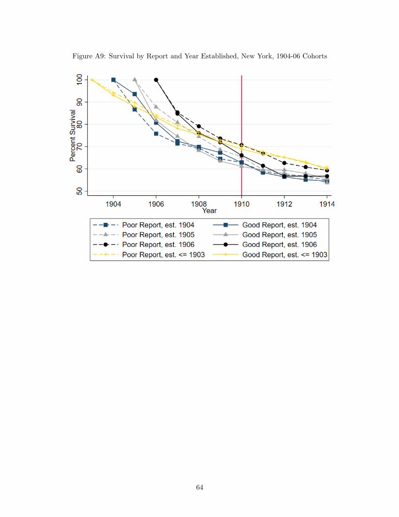
Figure A9: Survival by Report and Year Established, New York, 1904-06 Cohorts

64

Figure A10: Survival by Rating and Cohort, New Jersey, 1904-06

65

Figure A11: Survival by Rating and Cohort, Connecticut, 1904-06

66

Figure A12: Number of New Practices Recorded by Year

67

Figure A13: Survival Z Years, New York, Excl. Medical Centers

68

Figure A14: Survival Z Years, New York, Excluding Medical Centers

69

Figure A15: Survival Z Years, New York, Conditional on Survival 1 Year

70

Figure A16: Permutations Test for Si2 Coefficients

71

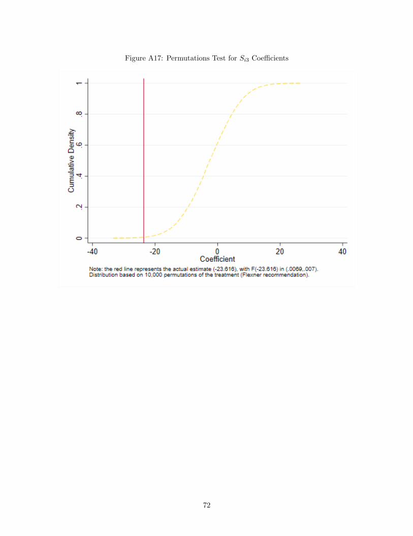
Figure A17: Permutations Test for Si3 Coefficients

72

Figure A18: Permutations Test for Si4 Coefficients

73

Figure A19: Permutations Test for Si5 Coefficients

74

Figure A20: Permutations Test for Pi,1910 Coefficients

75

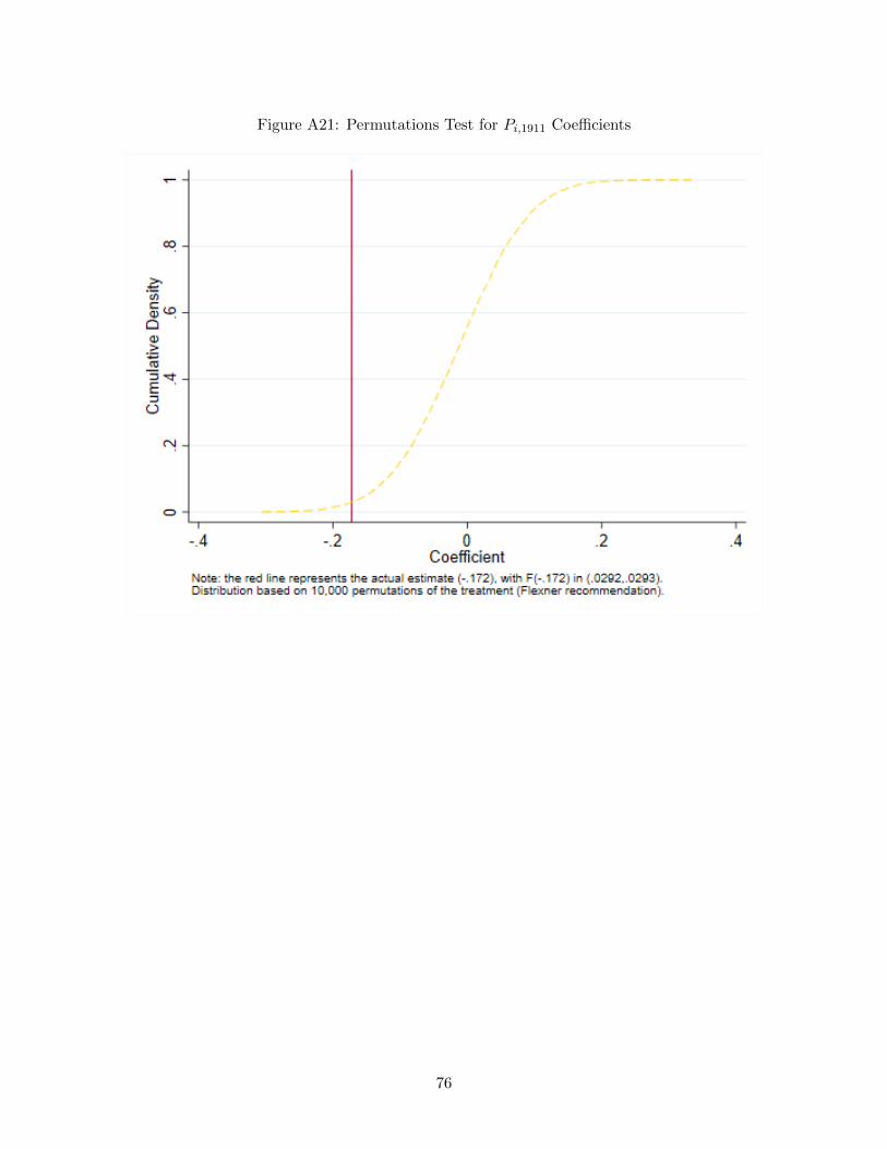
Figure A21: Permutations Test for Pi,1911 Coefficients

76

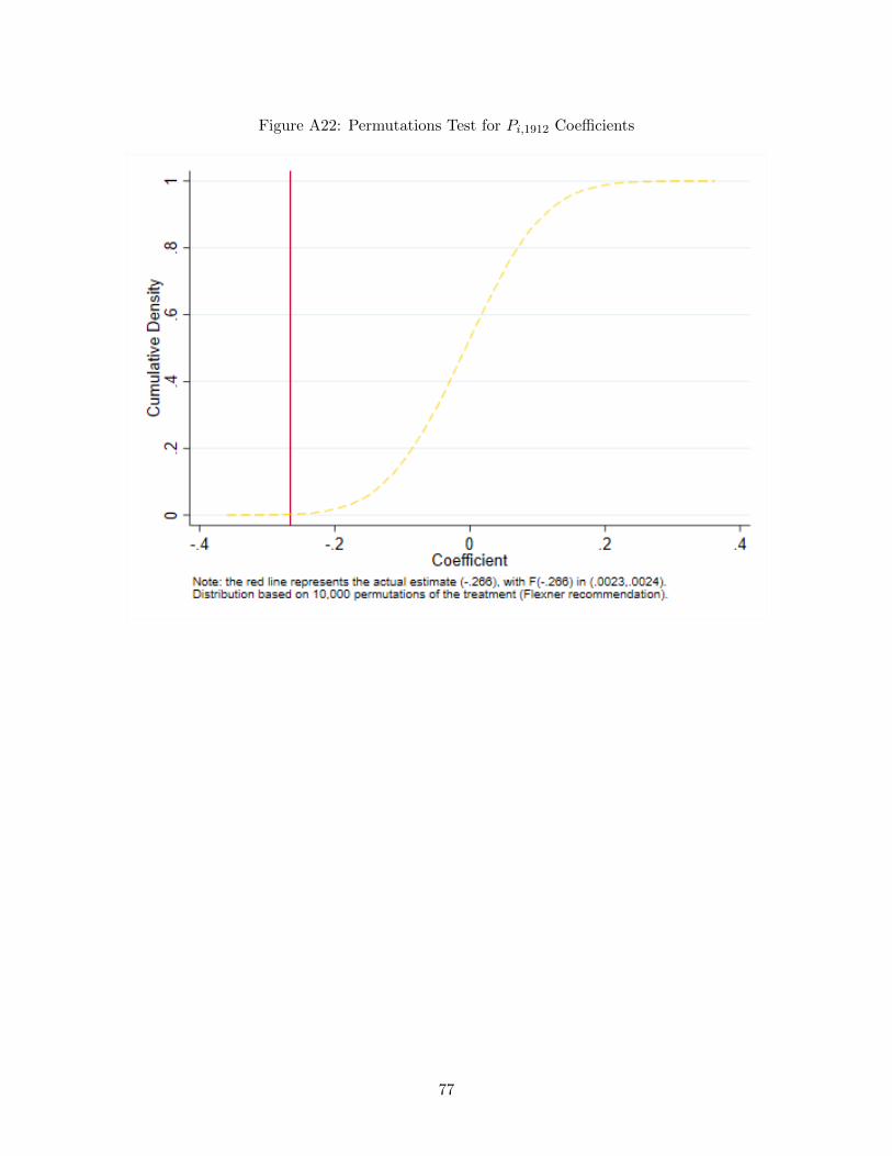
Figure A22: Permutations Test for Pi,1912 Coefficients

77

Figure A23: Permutations Test for Pi,1913 Coefficients

78

Figure A24: Permutations Test for Pi,1914 Coefficients

79

Figure A25: Percent of Failing Physicians that Switch Markets

80

Appendix B: Appendix Tables

Table B1: CME Rating in 1910, by School Type

School TypeHomeopathic Eclectic Women-only

A [4-Year Program] 6 1 1A [2-Year Program] 0 0 0B 4 4 1C 5 7 0Not Rated - Closed 0 0 1Total 15 12 3

Notes: One school rated B by the CME is listed in both the Homeo-pathic and Women-only columns.

81

Table B2: Flexner Ratings by State, 1909

Number of Physicians Percentage of PhysiciansNY NJ CT Panel NY NJ CT Panel

Direct Poor Rating 3,208 1,085 400 4,693 50.0 43.1 29.9 45.7Indirect Poor Rating 199 19 12 230 3.1 0.8 0.9 2.2Direct Good Rating 1,582 881 548 3,011 24.7 35.0 40.9 29.3Indirect Good Rating 942 352 200 1,494 14.7 14.0 14.9 14.5Half-School Rating 221 40 101 362 3.4 1.6 7.5 3.5Foreign School 62 69 27 158 1.0 2.7 2.0 1.5Closed prior to Flexner 151 70 48 269 2.4 2.8 3.6 2.6Licensed by Exam. Board 35 2 3 40 0.5 0.1 0.2 0.4Cannot be determined 11 2 1 14 0.2 0.1 0.1 0.1

TOTAL 6,411 2,520 1,340 10,271 100.0 100.0 100.0 100.0

82

Table B3: Distribution of Physician-Years by Medical School

Inst. ID New York New Jersey Connecticut PanelDirect: N Y N Y N Y N Y Total %103 10,264 780 4,079 518 2,225 124 16,568 1,422 17,990 14.9100 992 12,768 36 81 28 136 1,056 12,985 14,041 11.6101 0 6,224 0 4,640 0 1,900 0 12,764 12,764 10.598 0 10,764 0 215 0 207 0 11,186 11,186 9.2130 0 1,450 0 3,633 0 332 0 5,415 5,415 4.5107 0 3,265 0 1,369 0 735 0 5,369 5,369 4.4131 0 706 0 3,490 0 400 0 4,596 4,596 3.8108 307 4,022 7 42 17 0 331 4,064 4,395 3.699 0 2,302 0 820 0 550 0 3,672 3,672 3.017 0 258 0 173 0 3,100 0 3,531 3,531 2.9134 39 1,041 8 1,915 4 310 51 3,266 3,317 2.7155 0 2,201 0 262 0 781 0 3,244 3,244 2.7Closed 1,804 0 813 0 583 0 3,200 0 3,200 2.662 12 900 0 783 0 413 12 2,096 2,108 1.773 0 1,689 0 211 0 115 0 2,015 2,015 1.764 0 799 0 803 0 305 0 1,907 1,907 1.6Foreign 744 0 753 0 362 0 1,859 0 1,859 1.5102 0 1,097 0 408 0 94 0 1,599 1,599 1.3121 508 648 24 76 3 36 535 760 1,295 1.1106 0 820 0 146 0 269 0 1,235 1,235 1.040 274 622 20 161 7 98 301 881 1,182 1.0132 0 116 0 870 0 79 0 1,065 1,065 0.9135 0 312 0 444 0 190 0 946 946 0.8167 651 133 71 0 65 25 787 158 945 0.868 0 430 0 82 0 362 0 874 874 0.7168 43 607 12 57 10 86 65 750 815 0.797 0 343 0 131 0 327 0 801 801 0.7165 39 655 0 35 0 22 39 712 751 0.6119 0 562 0 48 2 98 2 708 710 0.6105 0 280 0 273 0 49 0 602 602 0.561 0 359 0 58 0 165 0 582 582 0.563 0 240 0 239 0 85 0 564 564 0.570 8 192 0 38 0 230 8 460 468 0.455 124 26 26 54 34 16 184 96 280 0.2State Board 190 0 30 0 43 0 263 0 263 0.228 0 168 0 66 0 24 0 258 258 0.2118 170 0 41 0 38 0 249 0 249 0.219 0 134 0 57 0 48 0 239 239 0.2122 0 198 0 12 0 23 0 233 233 0.2LIC*223 216 0 2 0 0 0 218 0 218 0.2156 0 76 0 87 0 51 0 214 214 0.2120 0 203 0 8 0 0 0 211 211 0.260 0 73 0 50 0 84 0 207 207 0.274 0 185 0 5 0 12 0 202 202 0.276 74 99 0 28 0 0 74 127 201 0.2124 98 27 32 0 36 0 166 27 193 0.218 111 31 13 11 12 9 136 51 187 0.229 0 137 0 18 0 24 0 179 179 0.169 0 74 0 9 0 77 0 160 160 0.1169 0 75 0 0 0 84 0 159 159 0.1

83

20 0 44 0 113 0 0 0 157 157 0.1123 79 11 24 6 0 13 103 30 133 0.130 0 72 0 23 0 31 0 126 126 0.139 0 69 0 32 5 12 5 113 118 0.165 0 51 0 43 0 7 0 101 101 0.171 0 36 0 44 0 20 0 100 100 0.132 0 63 0 0 0 28 0 91 91 0.166 0 0 0 18 0 70 0 88 88 0.1170 0 60 0 0 0 26 0 86 86 0.187 16 19 13 0 12 16 41 35 76 0.167 32 0 10 14 16 0 58 14 72 0.1CBV 53 0 18 0 1 0 72 0 72 0.1166 0 59 0 1 0 0 0 60 60 0.078 0 12 0 11 8 28 8 51 59 0.0n/a 45 0 13 0 0 0 58 0 58 0.015 35 6 0 5 11 0 46 11 57 0.046 4 22 7 0 17 0 28 22 50 0.0125 0 36 0 0 0 12 0 48 48 0.058 0 25 0 4 0 12 0 41 41 0.033 or 75 0 27 0 10 0 0 0 37 37 0.035 0 6 0 30 0 0 0 36 36 0.050 0 36 0 0 0 0 0 36 36 0.077 0 24 0 0 0 12 0 36 36 0.0157 0 12 0 15 0 7 0 34 34 0.0116 0 0 0 33 0 0 0 33 33 0.0147 0 7 0 24 0 0 0 31 31 0.027 0 14 0 3 0 12 0 29 29 0.0161 0 5 0 0 0 23 0 28 28 0.048 24 3 0 0 0 0 24 3 27 0.0158 0 0 0 12 0 14 0 26 26 0.0148 4 7 12 2 0 0 16 9 25 0.051 0 18 0 7 0 0 0 25 25 0.0139 0 5 0 7 0 12 0 24 24 0.052 24 0 0 0 0 0 24 0 24 0.088 12 4 7 0 0 0 19 4 23 0.012 13 0 0 0 5 0 18 0 18 0.023 4 7 1 0 6 0 11 7 18 0.094 0 0 0 12 5 0 5 12 17 0.0104 0 12 0 3 0 1 0 16 16 0.0137 0 0 15 0 0 0 15 0 15 0.0164 0 1 0 12 0 0 0 13 13 0.0144 or 145 0 0 0 0 0 12 0 12 12 0.025 0 0 0 0 0 12 0 12 12 0.037 0 0 0 0 0 12 0 12 12 0.0122 or 123 12 0 0 0 0 0 12 0 12 0.0128 0 11 0 0 0 0 0 11 11 0.0150 0 0 0 10 0 0 0 10 10 0.031 or 47 0 1 0 6 0 3 0 10 10 0.0YOP 0 0 0 0 10 0 10 0 10 0.091 0 0 0 9 0 0 0 9 9 0.02 0 0 0 0 0 7 0 7 7 0.0162 0 5 0 0 0 0 0 5 5 0.06 or 11 0 2 0 3 0 0 0 5 5 0.0DROP 0 0 5 0 0 0 5 0 5 0.0

84

54 0 0 0 0 0 4 0 4 4 0.0153 0 0 0 3 0 0 0 3 3 0.082 0 2 0 0 0 0 0 2 2 0.0Total 17,025 58,885 6,092 22,941 3,565 12,481 26,682 94,307 120,989 100.0

85

Table B4: Flexner Rating and Sect by Schools Present in Dataset

ID Rating Sect Institution City State2 Poor Regular Medical Department of the Uni-

versity of AlabamaMobile Alabama

12 Half Regular Leland Stanford Junior Univer-sity School of Medicine, on theCooper Medical College Founda-tion

San Francisco California

15 Poor Regular Denver and Gross College ofMedicine

Denver Colorado

17 Good Regular Yale Medical School New Haven Connecticut18 Poor Regular George Washington University,

Department of MedicineWashington District of Columbia

19 Poor Regular Georgetown University School ofMedicine

Washington District of Columbia

20 Good Primarily Black Howard University Medical Col-lege

Washington District of Columbia

23 Good Regular Atlanta College of Physiciansand Surgeons

Atlanta Georgia

25 Poor Eclectic Georgia College of EclecticMedicine and Surgery

Atlanta Georgia

27 Poor Regular Medical College of Georgia Augusta Georgia28 Good Regular Rush Medical College Chicago Illinois29 Good Regular Northwestern University Medi-

cal DepartmentChicago Illinois

30 Good Regular College of Physicians and Sur-geons

Chicago Illinois

32 Poor Eclectic Bennett Medical College Chicago Illinois35 Poor Regular Illinois Medical College Chicago Illinois37 Poor Not Matched National Medical University Chicago Illinois39 Poor Homeopathic Hering Medical College Chicago Illinois40 Poor Homeopathic Hahnemann Medical College Chicago Illinois46 Good Regular Indiana University School of

MedicineBloomington-Indianapolis

Indiana

48 Poor Eclectic Drake University College ofMedicine

Des Moines Iowa

50 Good Regular State University of Iowa Collegeof Medicine

Iowa City Iowa

51 Poor Homeopathic State University of Iowa Collegeof Homeopathic Medicine

Iowa City Iowa

52 Good Regular University of Kansas School ofMedicine

Lawrence-Rosedale;Suburb of bothKansas Cities

Kansas

54 Poor Regular Kansas Medical College Topeka Kansas55 Poor Regular University of Louisville Medical

DepartmentLouisville Kentucky

58 Good Regular Medical Department of the Tu-lane University of Louisiana

New Orleans Louisiana

60 Half Regular Medical School of Maine Brunswick-Portland

Maine

61 Good Regular Medical Department of theJohns Hopkins University

Baltimore Maryland

86

62 Poor Regular College of Physicians and Sur-geons

Baltimore Maryland

63 Poor Regular University of Maryland School ofMedicine

Baltimore Maryland

64 Poor Regular Baltimore Medical College Baltimore Maryland65 Poor Women-only Woman’s Medical College of

BaltimoreBaltimore Maryland

66 Poor Regular Maryland Medical College Baltimore Maryland67 Poor Homeopathic Atlantic Medical College Baltimore Maryland68 Good Regular Medical School of Harvard Uni-

versityBoston Massachusetts

69 Poor Regular Tufts College Medical School Boston Massachusetts70 Poor Homeopathic Boston University School of

MedicineBoston Massachusetts

71 Poor Regular College of Physicians and Sur-geons

Boston Massachusetts

73 Good Regular University of Michigan Depart-ment of Medicine and Surgery

Ann Arbor Michigan

74 Poor Homeopathic University of Michigan Homeo-pathic College

Ann Arbor Michigan

76 Poor Regular Detroit College of Medicine Detroit Michigan77 Poor Homeopathic Detroit Homeopathic College Detroit Michigan78 Good Regular University of Minnesota College

of Medicine and SurgeryMinneapolis-St.Paul

Minnesota

82 Poor Regular University Medical College Kansas City Missouri87 Good Regular Washington University Medical

DepartmentSt. Louis Missouri

88 Poor Regular St. Louis University St. Louis Missouri91 Poor Eclectic American Medical College St. Louis Missouri94 Good Regular College of Medicine, University

of NebraskaLincoln-Omaha Nebraska

97 Half Regular Dartmouth Medical School Hanover New Hampshire98 Poor Regular Albany Medical College Albany New York99 Poor Regular Long Island College Hospital Brooklyn New York100 Poor Regular University of Buffalo Medical

DepartmentBuffalo New York

101 Good Regular College of Physicians and Sur-geons

New York New York

102 Good Regular Cornell University Medical Col-lege

New York New York

103 Good Regular University and Bellevue HospitalMedical College

New York New York

104 Poor Regular Fordham University School ofMedicine

New York New York

105 Poor Women & Hom. New York Medical College andHospital for Women

New York New York

106 Poor Eclectic Eclectic Medical College New York New York107 Poor Homeopathic New York Homeopathic Medical

College and Flower HospitalNew York New York

108 Good Regular College of Medicine, SyracuseUniversity

Syracuse New York

116 Poor Primarily Black Leonard Medical School Raleigh North Carolina118 Good Regular Ohio-Miami Medical College of

the University of CincinnatiCincinnati Ohio

87

119 Poor Eclectic Eclectic Medical Institute Cincinnati Ohio120 Poor Homeopathic Pulte Medical College Cincinnati Ohio121 Poor Homeopathic Cleveland Homeopathic Medical

CollegeCleveland Ohio

122 Good Regular Western Reserve UniversityMedical Department

Cleveland Ohio

123 Poor Regular College of Physicians and Sur-geons

Cleveland Ohio

124 Poor Regular Starling-Ohio Medical College Columbus Ohio125 Poor Regular Toledo Medical College Toledo Ohio128 Poor Regular University of Oregon Medical

DepartmentPortland Oregon

130 Good Regular University of Pennsylvania De-partment of Medicine

Philadelphia Pennsylvania

131 Poor Regular Jefferson Medical College Philadelphia Pennsylvania132 Poor Regular Medico-Chirurgical College of

PhiladelphiaPhiladelphia Pennsylvania

134 Poor Homeopathic Hahnemann Medical Collegeand Hospital

Philadelphia Pennsylvania

135 Poor Women-only Woman’s Medical College ofPennsylvania

Philadelphia Pennsylvania

137 Good Regular University of Pittsburgh, Medi-cal Department

Pittsburgh Pennsylvania

139 Poor Regular Medical College of the State ofSouth Carolina

Charleston South Carolina

147 Good Regular Vanderbilt University MedicalDepartment

Nashville Tennessee

148 Poor Regular Universities of Nashville andTennessee Medical Department

Nashville Tennessee

150 Poor Regular Baylor University College ofMedicine

Dallas Texas

153 Good Regular University of Texas, Departmentof Medicine

Galveston Texas

155 Half Regular University of Vermont College ofMedicine

Burlington Vermont

156 Good Regular University of Virginia, Depart-ment of Medicine

Charlottesville Virginia

157 Poor Regular Medical College of Virginia Richmond Virginia158 Poor Regular University College of Medicine Richmond Virginia161 Poor Regular Milwaukee Medical College Milwaukee Wisconsin162 Poor Regular Wisconsin College of Physicians

and SurgeonsMilwaukee Wisconsin

164 Poor Regular Halifax Medical College Halifax Nova Scotia165 Good Regular Medical Department of Queen’s

UniversityKingston Ontario

166 Poor Regular Western University Medical De-partment

London Ontario

167 Good Regular University of Toronto Faculty ofMedicine

Toronto Ontario

168 Good Regular McGill University Medical Fac-ulty

Montreal Quebec

169 Poor Regular Laval University Medical De-partment

Montreal Quebec

88

170 Good Regular Laval University Medical De-partment

Quebec Quebec

89

Table B5: Additional Designations

ID Rating Sect Description6 or 11 Cannot be Determined Regular University of California: Clinical Department [Los An-

geles; Poor Rating] OR University of California Med-ical Department [San Francisco; Good Rating]

31 or 47 Poor Eclectic Chicago College of Medicine and Surgery [Chicago, IL]OR Valparaiso University [Valparaiso, Indiana]

33 or 75 Poor Regular American Medical Missionary College [Chicago, IL]OR American Medical Missionary College [BattleCreek, MI]

122 or 123 Cannot be Determined Regular Western Reserve University Medical Department[Cleveland, OH; Good Rating] OR College of Physi-cians and Surgeons [Cleveland, OH; Poor Rating]

144 or 145 Poor Regular College of Physicians and Surgeons [Memphis, TN] ORMemphis Hospital Medical College [Memphis, TN]

CBV Cannot be Determined n/a ”Cannot Be Validated” [Uncertain Match]Closed Closed Prior to Report n/a School Closed Prior to Flexner’s InspectionsDROP Cannot be Determined n/a Degree Listed Determined to not be Undergraduate

Medical Degree.Foreign Foreign n/a Foreign Medical School. Not evaluated by Flexner in

1910 Report.LIC*223 Lic. by Exam. Board n/a Degree Listed as ”UNIV. STATE N.Y.” or similar in

local medical directories. This was determined mostlikely to refer to a State Board. In a small number ofcases, this may refer to ”Univ. N.Y.” which mergedinto institution id 103 in 1898.

State Board Lic. by Exam. Board n/a Practicing medicine on the basis of approval by StateBoard.

YOP Cannot be Determined n/a Allowed to practice based on ”Years of Practice” laws.n/a Cannot be Determined n/a No degree listed.

90

Table B6: School Type, Direct Poor Rating, 1909

Number of Physicians Percentage of PhysiciansNY NJ CT Panel NY NJ CT Panel

Regular Med. Schools 2,510 675 220 3,405 78.2 62.2 55.1 72.6Homeopathic Med. Schools 553 341 127 1,021 17.2 31.4 31.8 21.8Eclectic Med. Schools 115 19 34 168 3.6 1.8 8.5 3.6Black Med. Schools 0 3 0 3 0.0 0.3 0.0 0.1Women-only Med. Schools 53 72 23 148 1.7 6.6 5.8 3.2Women’s Hom. Med. Schools 23 25 5 53 0.7 2.3 1.3 1.1

All Direct Poor Ratings 3,208 1,085 399 4,692 100.0 100.0 100.0 100.0

Notes: (i) A single observation in Connecticut could not be allocated to a school type; (ii) Physicians thatattended Women’s Homeopathic Medical Schools are included in three rows.

91

Table B7: School Type, Direct Good Rating, 1909

Number of Physicians Percentage of PhysiciansNY NJ CT Panel NY NJ CT Panel

Regular Med. Schools 1,579 871 548 2,998 99.8 98.9 100.0 99.6Homeopathic Med. Schools 0 0 0 0 0.0 0.0 0.0 0.0Eclectic Med. Schools 0 0 0 0 0.0 0.0 0.0 0.0Black Med. Schools 3 10 0 13 0.2 1.1 0.0 0.4Women-only Med. Schools 0 0 0 0 0.0 0.0 0.0 0.0Women’s Hom. Med. Schools 0 0 0 0 0.0 0.0 0.0 0.0

All Direct Good Ratings 1,582 881 548 3,011 100.0 100.0 100.0 100.0

92

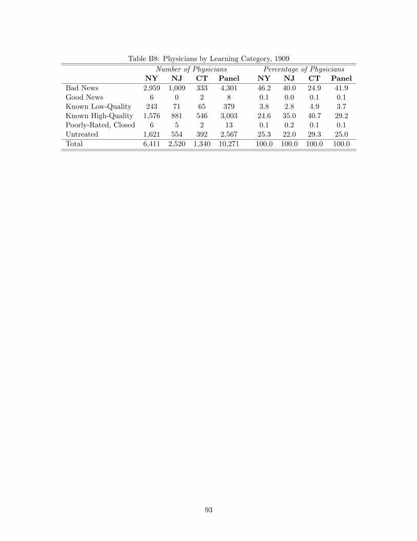
Table B8: Physicians by Learning Category, 1909

Number of Physicians Percentage of PhysiciansNY NJ CT Panel NY NJ CT Panel

Bad News 2,959 1,009 333 4,301 46.2 40.0 24.9 41.9Good News 6 0 2 8 0.1 0.0 0.1 0.1Known Low-Quality 243 71 65 379 3.8 2.8 4.9 3.7Known High-Quality 1,576 881 546 3,003 24.6 35.0 40.7 29.2Poorly-Rated, Closed 6 5 2 13 0.1 0.2 0.1 0.1Untreated 1,621 554 392 2,567 25.3 22.0 29.3 25.0

Total 6,411 2,520 1,340 10,271 100.0 100.0 100.0 100.0

93

Table B9: Ayer Data, Newspaper Counts

New York New Jersey Connecticut Panel

All Newspapers:Daily 146 48 36 230Weekly 914 320 129 1,363Total 1,062 372 167 1,601

General Newspapers:Daily 136 47 34 217Weekly 871 299 117 1,287Total 876 301 118 1,295

94

Tab

leB

10:

Nu

mb

erof

Physi

cian

sby

Fle

xn

erR

atin

gan

dY

ear,

Tri

-Sta

teA

rea

1903

1904

1905

1906

1907

1908

1909

1910

1911

1912

1913

1914

Pan

el

Dir

ect

Poor

Rat

ing

3,93

74,

151

4,2

52

4,3

25

4,4

00

4,5

42

4,6

93

4,7

74

4,8

18

4,847

4,9

21

5,0

13

54,6

73

Ind

irec

tP

oor

Rat

ing

246

252

248

241

236

231

230

225

221

223

222

221

2,7

96

Dir

ect

Good

Rat

ing

2,35

62,

526

2,6

25

2,6

99

2,7

68

2,9

03

3,0

11

3,1

15

3,2

28

3,282

3,3

88

3,4

76

35,3

77

Ind

irec

tG

ood

Rat

ing

1,65

41,

663

1,6

36

1,5

88

1,5

59

1,5

27

1,4

94

1,4

69

1,4

44

1,407

1,3

75

1,3

55

18,1

71

Hal

f-S

chool

Rat

ing

349

363

350

345

352

357

362

367

365

355

352

353

4,2

70

For

eign

Sch

ool

128

133

143

138

146

157

158

167

178

176

169

166

1,8

59

Clo

sed

pri

orto

Fle

xn

er28

830

6301

288

282

284

269

262

252

233

223

212

3,2

00

Lic

ense

dby

Exam

.B

oard

3538

44

43

40

40

40

41

41

40

40

39

481

Can

not

be

det

erm

ined

2217

14

10

15

12

14

14

11

11

12

10

162

Tota

l9,

015

9,44

99,6

13

9,6

77

9,7

98

10,0

53

10,2

71

10,4

34

10,5

58

10,5

74

10,7

02

10,8

45

120,9

89

95

Tab

leB

11:

Nu

mb

erof

Physi

cian

sby

Fle

xn

erR

atin

gan

dY

ear

1903

1904

1905

1906

1907

1908

1909

1910

1911

1912

1913

1914

Pan

el

Dir

ect

Poor

Rat

ing

2,28

32,

344

2,3

51

2,3

95

2,4

30

2,4

82

2,5

39

2,5

81

2,5

95

2,6

07

2,6

17

2,6

53

29,8

77

Ind

irec

tP

oor

Rat

ing

146

143

143

139

137

131

130

124

122

124

126

126

1,5

91

Dir

ect

Good

Rat

ing

1,01

41,

072

1,1

23

1,1

80

1,2

25

1,2

79

1,3

44

1,3

96

1,4

55

1,4

88

1,5

13

1,5

72

15,6

61

Ind

irec

tG

ood

Rat

ing

972

966

956

929

913

887

871

856

845

825

815

807

10,6

42

Hal

f-S

chool

Rat

ing

218

218

211

205

207

205

210

212

208

199

196

196

2,4

85

For

eign

Sch

ool

4344

43

41

46

43

43

44

44

46

41

40

518

Clo

sed

pri

orto

Fle

xn

er17

417

7170

159

152

149

140

134

126

113

106

99

1,6

99

Lic

ense

dby

Exam

.B

oard

2627

30

32

31

30

32

31

32

30

30

29

360

Can

not

be

det

erm

ined

98

75

86

77

66

54

78

Tota

l4,

885

4,999

5,0

34

5,0

85

5,1

49

5,2

12

5,3

16

5,3

85

5,4

33

5,4

38

5,4

49

5,5

26

62,9

11

96

Table B12: Weibull Model, Baseline, All Cohorts

(1) (2) (3) (4)

Poorly Rated 0.978 0.963(0.125) (0.346)

‘Bad News’ 0.943 0.955(0.123) (0.343)

Exp 0.994 1.032 0.994 1.032(0.0154) (0.0333) (0.0154) (0.0334)

Exp2 1.001*** 1.000 1.001*** 1.000(0.000298) (0.000821) (0.000297) (0.000825)

Shape Parameter 1.588*** 1.645*** 1.588*** 1.645***(0.0477) (0.0755) (0.0477) (0.0757)

Constant 0.00638*** 2.30e-09*** 0.00637*** 2.30e-09***(0.00155) (2.45e-09) (0.00156) (2.44e-09)

Market (3km-Roll) FE Y Y Y YCohort FE Y Y Y YIncl. Left-Censored Data Y N Y NLog-Likelihood -1,093.6 -301.3 -1,093.5 -301.3Pseudo-R2 0.089 0.147 0.089 0.147Years at Risk 12,077 2,718 12,077 2,718Clusters 101 73 101 73Failures 451 131 451 131Observations 1,414 422 1,414 422

Notes: Results presented are proportional hazards from the Weibull parametric survival model; values equal to1 indicate no difference in the hazard of practice failure, while values smaller than 1 are proportional decreases inhazard. Values larger than 1 represent proportional increases in the hazard of practice failure. The ‘Shape Parameter’represents p in the Weibull hazard function; larger values indicate increasing hazard over time. The ‘Constant’ givesbaseline hazard when no other variables are included. All columns are restricted to baseline restrictions: (i) theseare conditional hazards – only physicians surviving at least one year in local market m are included; (ii) only NYis included; (iii) medical centers are excluded; (iv) areas with population 100,000 or above are excluded; (v) onlyphysicians graduating from regular institutions still operating in 1909 are included; (vi) physicians must have enteredtheir market prior to the release of the Flexner Report to be included; (vii) only areas with a weekly general-contentnewspaper within 25km of the market are included; and (viii) markets where a specific degree is held by more thanone-third of physicians are excluded. Standard errors (in parentheses) are clustered at the 3km-rolling market level.Statistical significance is denoted by the following: *** (p-value < 0.01), ** (p-value < 0.05), and * (p-value < 0.10).

97

Table B13: Level Model, Linear Regression

Survival to Year Y = 1Y : 1910 1911 1912 1913 1914

Well-Rated 0.00505 0.00468 0.0241 0.0135 -0.00681(0.0180) (0.0233) (0.0266) (0.0250) (0.0274)

Poorly-Rated 0.0301* 0.0125 0.0140 -0.00224 -0.0208(0.0164) (0.0253) (0.0292) (0.0326) (0.0359)

Exp 0.00604** 0.00411 0.00309 0.000621 -0.000843(0.00298) (0.00329) (0.00332) (0.00387) (0.00424)

Exp2 -0.000210*** -0.000198** -0.000171** -0.000189* -0.000197*(7.66e-05) (8.21e-05) (8.28e-05) (0.000106) (0.000108)

Constant 1.009*** 1.049*** 0.839*** 0.683*** 0.724***(0.0246) (0.0356) (0.0331) (0.0311) (0.0372)

Market (3km-Roll) FE Y Y Y Y YCohort FE Y Y Y Y YR2 0.111 0.117 0.123 0.141 0.141Clusters 101 101 101 101 101Observations 1,212 1,212 1,212 1,212 1,212

Notes: Only physician-markets pairs observed in 1909 are included. All columns are restricted tobaseline restrictions: (i) only NY is included; (ii) medical centers are excluded; (iii) areas withpopulation 100,000 or above are excluded; (iv) only physicians graduating from regular institutionsstill operating in 1909 are included; (v) physicians must have entered their market prior to the releaseof the Flexner Report to be included; (vi) only areas with a weekly general-content newspaper within25km of the market are included; and (vii) markets where a specific degree is held by more than one-third of physicians are excluded. Experience is calculated based on year of market-entry. Standarderrors (in parentheses) are clustered at the 3km-rolling market level. Statistical significance is denotedby the following: *** (p-value < 0.01), ** (p-value < 0.05), and * (p-value < 0.10).

98

Table B14: Level Model with Bad News, Linear Regression

Survival to Year Y = 1Y : 1910 1911 1912 1913 1914

‘Bad News’ 0.0338* 0.0199 0.0106 -0.000482 -0.00258(0.0197) (0.0259) (0.0304) (0.0323) (0.0352)

CME: Rated A -0.00320 -0.0100 -0.00178 -0.00544 -0.0201(0.0184) (0.0222) (0.0265) (0.0238) (0.0250)

CME: Rated B/C -0.130 -0.176 -0.271* -0.222 -0.231*(0.106) (0.126) (0.143) (0.138) (0.136)

Exp 0.00569* 0.00358 0.00214 -6.64e-05 -0.00131(0.00307) (0.00330) (0.00341) (0.00403) (0.00433)

Exp2 -0.000204** -0.000188** -0.000153* -0.000176 -0.000188*(7.81e-05) (8.27e-05) (8.51e-05) (0.000109) (0.000110)

Constant 1.016*** 1.063*** 0.860*** 0.699*** 0.739***(0.0275) (0.0367) (0.0361) (0.0352) (0.0393)

Market (3km-Roll) FE Y Y Y Y YCohort FE Y Y Y Y YR2 0.116 0.121 0.129 0.144 0.144Clusters 101 101 101 101 101Observations 1,212 1,212 1,212 1,212 1,212

Notes: Only physician-markets pairs observed in 1909 are included. All columns are restricted tobaseline restrictions: (i) only NY is included; (ii) medical centers are excluded; (iii) areas withpopulation 100,000 or above are excluded; (iv) only physicians graduating from regular institutionsstill operating in 1909 are included; (v) physicians must have entered their market prior to the releaseof the Flexner Report to be included; (vi) only areas with a weekly general-content newspaper within25km of the market are included; and (vii) markets where a specific degree is held by more than one-third of physicians are excluded. Experience is calculated based on year of market-entry. Standarderrors (in parentheses) are clustered at the 3km-rolling market level. Statistical significance is denotedby the following: *** (p-value < 0.01), ** (p-value < 0.05), and * (p-value < 0.10).

99

Table B15: Level Model, CME Ratings, Simple Linear Regression

Survival to Year Y = 1Y : 1910 1911 1912 1913 1914

CME: Rated A 0.0135 -0.000206 0.00347 -0.00568 -0.0213(0.0145) (0.0195) (0.0238) (0.0228) (0.0251)

CME: Rated B/C -0.128 -0.174 -0.271* -0.222 -0.231*(0.105) (0.126) (0.143) (0.138) (0.135)

Exp 0.00606* 0.00379 0.00226 -7.16e-05 -0.00134(0.00310) (0.00335) (0.00344) (0.00399) (0.00426)

Exp2 -0.000211*** -0.000192** -0.000155* -0.000176 -0.000188*(7.85e-05) (8.30e-05) (8.49e-05) (0.000108) (0.000108)

Constant 1.000*** 1.053*** 0.855*** 0.700*** 0.740***(0.0268) (0.0376) (0.0372) (0.0336) (0.0389)

Market (3km-Roll) FE Y Y Y Y YCohort FE Y Y Y Y YR2 0.112 0.120 0.128 0.144 0.144Clusters 101 101 101 101 101Observations 1,212 1,212 1,212 1,212 1,212

Notes: Only physician-markets pairs observed in 1909 are included. All columns are restricted tobaseline restrictions: (i) only NY is included; (ii) medical centers are excluded; (iii) areas withpopulation 100,000 or above are excluded; (iv) only physicians graduating from regular institutionsstill operating in 1909 are included; (v) physicians must have entered their market prior to the releaseof the Flexner Report to be included; (vi) only areas with a weekly general-content newspaper within25km of the market are included; and (vii) markets where a specific degree is held by more than one-third of physicians are excluded. Experience is calculated based on year of market-entry. Standarderrors (in parentheses) are clustered at the 3km-rolling market level. Statistical significance is denotedby the following: *** (p-value < 0.01), ** (p-value < 0.05), and * (p-value < 0.10).

100

Table B16: Time-Varying Hazards, Cox Model, With Degree FE

Years: Interacted with: (1) (2) (3) (4) (5) (6)

Y ≥ 1910: All Physicians 0.978 1.005 1.042 0.781 0.781 0.820(0.275) (0.283) (0.295) (0.304) (0.304) (0.321)

Poorly Rated 1.113 1.356(0.270) (0.582)

‘Bad News’ 1.036 1.356(0.252) (0.582)

Well-Rated 0.937 1.127(0.226) (0.483)

n/a: Exp 0.996 0.996 0.996 1.010 1.010 1.009(0.0143) (0.0143) (0.0143) (0.0351) (0.0351) (0.0352)

Exp2 1.001*** 1.001*** 1.001*** 1.000 1.000 1.000(0.000274) (0.000274) (0.000272) (0.000801) (0.000801) (0.000812)

Market FE Y Y Y Y Y YCohort FE Y Y Y Y Y YDegree FE Y Y Y Y Y YIncl. L.-C. Data Y Y Y N N NLog-Likelihood -3,036.1 -3,036.2 -3,036.2 -694.4 -694.4 -694.6Pseudo-R2 0.037 0.037 0.037 0.087 0.087 0.087Years at Risk 12,057 12,057 12,057 2,718 2,718 2,718Clusters 101 101 101 73 73 73Failures 449 449 449 131 131 131Physicians 1,412 1,412 1,412 422 422 422Observations 13,345 13,345 13,345 3,099 3,099 3,099

Notes: φ denotes entry year cohort for the physician-market pair. Results presented are proportional hazards fromthe Cox Proportional Hazards model; values equal to 1 indicate no difference in the hazard of practice failure, whilevalues smaller than 1 are proportional decreases in hazard. Values larger than 1 represent proportional increases inthe hazard of practice failure. All columns are restricted to baseline restrictions: (i) these are conditional hazards– only physicians surviving at least one year in local market m are included; (ii) only NY is included; (iii) medicalcenters are excluded; (iv) areas with population 100,000 or above are excluded; (v) only physicians graduating fromregular institutions still operating in 1909 are included; (vi) physicians must have entered their market prior to therelease of the Flexner Report to be included; (vii) only areas with a weekly general-content newspaper within 25kmof the market are included; and (viii) markets where a specific degree is held by more than one-third of physiciansare excluded. Market definition is baseline: 3km-rolling markets. Standard errors (in parentheses) are clustered atthe 3km-rolling market level. Statistical significance is denoted by the following: *** (p-value < 0.01), ** (p-value< 0.05), and * (p-value < 0.10).

101

Table B17: Time-Varying Hazards, Weibull Model, Baseline Sample

Years: Interacted with: (1) (2) (3) (4) (5) (6)

Y ≥ 1903: Poorly Rated 0.904 0.603(0.146) (0.228)

‘Bad News’ 0.895 0.655(0.140) (0.243)

Well-Rated 1.017 1.094(0.183) (0.409)

Y ≥ 1910: All Physicians 0.414*** 0.422*** 0.446*** 0.216*** 0.227*** 0.283***(0.0610) (0.0621) (0.0568) (0.0782) (0.0851) (0.103)

Poorly Rated 1.148 2.047*(0.288) (0.836)

‘Bad News’ 1.091 1.807(0.270) (0.755)

Well-Rated 0.922 0.951(0.221) (0.346)

n/a: Exp 0.993 0.993 0.993 1.029 1.029 1.032(0.0156) (0.0156) (0.0157) (0.0312) (0.0314) (0.0276)

Exp2 1.001*** 1.001*** 1.001*** 1.000 1.000 1.000(0.000302) (0.000302) (0.000307) (0.000755) (0.000765) (0.000666)

Shape Parameter 2.034*** 2.034*** 2.035*** 2.279*** 2.275*** 2.274***(0.0668) (0.0669) (0.0666) (0.183) (0.182) (0.183)

Constant 0.00373*** 0.00368*** 0.00367*** 4.48e-10*** 4.37e-10*** 3.58e-10***(0.00101) (0.00100) (0.00109) (4.97e-10) (4.84e-10) (4.03e-10)

Market FE Y Y Y Y Y YCohort FE Y Y Y Y Y YDegree FE N N N N N NIncl. L.-C. Data Y Y Y N N NLog-Likelihood -1,074.5 -1,074.5 -1,074.6 -291.5 -292.0 -292.9Pseudo-R2 0.104 0.104 0.104 0.175 0.174 0.171Years at Risk 12,057 12,057 12,057 2,718 2,718 2,718Clusters 101 101 101 73 73 73Failures 449 449 449 131 131 131Physicians 1,412 1,412 1,412 422 422 422Observations 13,345 13,345 13,345 3,099 3,099 3,099

Notes: φ denotes entry year cohort for the physician-market pair. Results presented are proportional hazards fromthe Weibull parametric survival model; values equal to 1 indicate no difference in the hazard of practice failure, whilevalues smaller than 1 are proportional decreases in hazard. Values larger than 1 represent proportional increasesin the hazard of practice failure. The ‘Shape Parameter’ represents p in the Weibull hazard function; larger valuesindicate increasing hazard over time. The ‘Constant’ gives baseline hazard when no other variables are included. Allcolumns are restricted to baseline restrictions: (i) these are conditional hazards – only physicians surviving at leastone year in local market m are included; (ii) only NY is included; (iii) medical centers are excluded; (iv) areas withpopulation 100,000 or above are excluded; (v) only physicians graduating from regular institutions still operatingin 1909 are included; (vi) physicians must have entered their market prior to the release of the Flexner Report tobe included; (vii) only areas with a weekly general-content newspaper within 25km of the market are included; and(viii) markets where a specific degree is held by more than one-third of physicians are excluded. Market definitionis baseline: 3km-rolling markets. Standard errors (in parentheses) are clustered at the 3km-rolling market level.Statistical significance is denoted by the following: *** (p-value < 0.01), ** (p-value < 0.05), and * (p-value < 0.10).

102

Table B18: Time-Varying Hazards, Weibull Model, With Degree FE

Years: Interacted with: (1) (2) (3) (4) (5) (6)

Y ≥ 1910: All Physicians 0.415*** 0.427*** 0.443*** 0.236*** 0.251*** 0.275***(0.0620) (0.0644) (0.0585) (0.0860) (0.0924) (0.0968)

Poorly Rated 1.143 1.731(0.288) (0.778)

‘Bad News’ 1.058 1.478(0.267) (0.658)

Well-Rated 0.943 1.098(0.231) (0.430)

n/a: Exp 0.992 0.992 0.992 1.009 1.009 1.008(0.0155) (0.0155) (0.0155) (0.0413) (0.0415) (0.0415)

Exp2 1.001*** 1.001*** 1.001*** 1.000 1.000 1.000(0.000316) (0.000315) (0.000315) (0.00101) (0.00102) (0.00103)

Shape Parameter 2.069*** 2.069*** 2.070*** 2.391*** 2.390*** 2.391***(0.0704) (0.0705) (0.0701) (0.197) (0.196) (0.197)

Constant 0.00427*** 0.00420*** 0.00413*** 6.15e-11*** 6.75e-11*** 8.82e-11***(0.00594) (0.00585) (0.00567) (8.57e-11) (9.42e-11) (1.24e-10)

Market FE Y Y Y Y Y YCohort FE Y Y Y Y Y YDegree FE N N N N N NIncl. L.-C. Data Y Y Y N N NLog-Likelihood -1,049.8 -1,050.0 -1,050.0 -266.1 -266.5 -266.9Pseudo-R2 0.124 0.124 0.124 0.247 0.246 0.245Years at Risk 12,057 12,057 12,057 2,718 2,718 2,718Clusters 101 101 101 73 73 73Failures 449 449 449 131 131 131Physicians 1,412 1,412 1,412 422 422 422Observations 13,345 13,345 13,345 3,099 3,099 3,099

Notes: φ denotes entry year cohort for the physician-market pair. Results presented are proportional hazards fromthe Weibull parametric survival model; values equal to 1 indicate no difference in the hazard of practice failure, whilevalues smaller than 1 are proportional decreases in hazard. Values larger than 1 represent proportional increasesin the hazard of practice failure. The ‘Shape Parameter’ represents p in the Weibull hazard function; larger valuesindicate increasing hazard over time. The ‘Constant’ gives baseline hazard when no other variables are included. Allcolumns are restricted to baseline restrictions: (i) these are conditional hazards – only physicians surviving at leastone year in local market m are included; (ii) only NY is included; (iii) medical centers are excluded; (iv) areas withpopulation 100,000 or above are excluded; (v) only physicians graduating from regular institutions still operatingin 1909 are included; (vi) physicians must have entered their market prior to the release of the Flexner Report tobe included; (vii) only areas with a weekly general-content newspaper within 25km of the market are included; and(viii) markets where a specific degree is held by more than one-third of physicians are excluded. Market definitionis baseline: 3km-rolling markets. Standard errors (in parentheses) are clustered at the 3km-rolling market level.Statistical significance is denoted by the following: *** (p-value < 0.01), ** (p-value < 0.05), and * (p-value < 0.10).

103

Table B19: Cox Model, Difference-in-Difference, By Newsiness, Incl. Left-Censored Data

(1) (2) (3) (4) (5)

Poorly Rated (φ ≥ 1904) 0.761 0.669(0.222) (0.220)

Poorly Rated (φ ∈ [1908,1909]) 3.023*** 4.499***(1.136) (1.820)

CME: Rated B/C (φ ≥ 1904) 1.003 0.942(1.495) (1.405)

CME: Rated B/C (φ ∈ [1908,1909]) 0.607 1.053(1.893) (3.261)

‘Bad News’ (φ ≥ 1904) 0.754 0.754(0.221) (0.221)

‘Bad News’ (φ ∈ [1908,1909]) 3.115*** 3.120***(1.094) (1.140)

Exp 0.998 0.997 1.010 0.998 0.998(0.0143) (0.0143) (0.0176) (0.0143) (0.0144)

Exp2 1.001*** 1.001*** 1.001* 1.001*** 1.001***(0.000270) (0.000273) (0.000317) (0.000271) (0.000271)

Market (3km-Roll) FE Y Y Y Y YCohort FE Y Y Y Y YDegree FE Y Y Y Y YIncl. Left-Censored Data Y Y Y Y YRest. to CME Rating: N N Y N NLog-Likelihood -3,048.0 -3,050.9 -2,060.3 -3,047.8 -3,047.8Pseudo-R2 0.037 0.036 0.050 0.037 0.037Years at Risk 12,077 12,077 8,699 12,077 12,077Clusters 101 101 101 101 101Failures 451 451 324 451 451Observations 1,414 1,414 1,034 1,414 1,414

Notes: φ denotes entry year cohort for the physician-market pair. Results presented are proportional hazards fromthe Cox Proportional Hazards model; values equal to 1 indicate no difference in the hazard of practice failure, whilevalues smaller than 1 are proportional decreases in hazard. Values larger than 1 represent proportional increases inthe hazard of practice failure. All columns are restricted to baseline restrictions: (i) these are conditional hazards– only physicians surviving at least one year in local market m are included; (ii) only NY is included; (iii) medicalcenters are excluded; (iv) areas with population 100,000 or above are excluded; (v) only physicians graduating fromregular institutions still operating in 1909 are included; (vi) physicians must have entered their market prior to therelease of the Flexner Report to be included; (vii) only areas with a weekly general-content newspaper within 25kmof the market are included; and (viii) markets where a specific degree is held by more than one-third of physiciansare excluded. Column (3) additionally restricts the sample to physicians who attended institutions that received arating of A from the CME. Standard errors (in parentheses) are clustered at the 3km-rolling market level. Statisticalsignificance is denoted by the following: *** (p-value < 0.01), ** (p-value < 0.05), and * (p-value < 0.10).

104

Table B20: Cox Model, Difference-in-Difference, By Newsiness, Excl. Left-Censored Data

(1) (2) (3) (4) (5)

Poorly Rated (φ ∈ [1908,1909]) 2.901** 4.721***(1.347) (2.455)

CME: Rated B/C (φ ∈ [1908,1909]) 0.108*** 0.125***(0.0756) (0.0930)

‘Bad News’ (φ ∈ [1908,1909]) 2.901** 2.901**(1.347) (1.347)

Exp 1.012 1.010 1.023 1.012 1.012(0.0355) (0.0357) (0.0374) (0.0355) (0.0355)

Exp2 1.000 1.000 1.000 1.000 1.000(0.000814) (0.000827) (0.000778) (0.000814) (0.000814)

Market (3km-Roll) FE Y Y Y Y YCohort FE Y Y Y Y YDegree FE Y Y Y Y YIncl. Left-Censored Data N N N N NRest. to CME Rating: N N Y N NLog-Likelihood -692.7 -694.7 -556.2 -692.7 -692.7Pseudo-R2 0.089 0.086 0.101 0.089 0.089Years at Risk 2,718 2,718 2,305 2,718 2,718Clusters 73 73 70 73 73Failures 131 131 110 131 131Observations 422 422 359 422 422

Notes: φ denotes entry year cohort for the physician-market pair. Results presented are proportional hazards fromthe Cox Proportional Hazards model; values equal to 1 indicate no difference in the hazard of practice failure, whilevalues smaller than 1 are proportional decreases in hazard. Values larger than 1 represent proportional increases inthe hazard of practice failure. All columns are restricted to baseline restrictions: (i) these are conditional hazards– only physicians surviving at least one year in local market m are included; (ii) only NY is included; (iii) medicalcenters are excluded; (iv) areas with population 100,000 or above are excluded; (v) only physicians graduating fromregular institutions still operating in 1909 are included; (vi) physicians must have entered their market prior to therelease of the Flexner Report to be included; (vii) only areas with a weekly general-content newspaper within 25kmof the market are included; and (viii) markets where a specific degree is held by more than one-third of physiciansare excluded. Column (3) additionally restricts the sample to physicians who attended institutions that received arating of A from the CME. Standard errors (in parentheses) are clustered at the 3km-rolling market level. Statisticalsignificance is denoted by the following: *** (p-value < 0.01), ** (p-value < 0.05), and * (p-value < 0.10).

105

Table B21: Weibull Model, Difference-in-Difference, By Newsiness, Incl. Left-Censored Data

(1) (2) (3) (4) (5)

Poorly Rated (φ ≥ 1904) 0.742 0.643(0.235) (0.231)

Poorly Rated (φ ∈ [1908,1909]) 3.276*** 5.076***(1.320) (2.253)

CME: Rated B/C (φ ≥ 1904) 1.038 0.973(1.656) (1.560)

CME: Rated B/C (φ ∈ [1908,1909]) 0.606 1.078(2.765) (4.934)

‘Bad News’ (φ ≥ 1904) 0.736 0.735(0.232) (0.233)

‘Bad News’ (φ ∈ [1908,1909]) 3.358*** 3.364***(1.258) (1.303)

Exp 0.994 0.993 1.006 0.994 0.994(0.0153) (0.0153) (0.0190) (0.0153) (0.0153)

Exp2 1.001*** 1.001*** 1.001** 1.001*** 1.001***(0.000304) (0.000309) (0.000358) (0.000304) (0.000305)

Shape Parameter 1.625*** 1.621*** 1.683*** 1.625*** 1.625***(0.0493) (0.0495) (0.0587) (0.0499) (0.0499)

Constant 0.00695*** 0.00719*** 0.00236*** 0.00695*** 0.00695***(0.00934) (0.00976) (0.000844) (0.00937) (0.00936)

Market (3km-Roll) FE Y Y Y Y YCohort FE Y Y Y Y YDegree FE Y Y Y Y YIncl. Left-Censored Data Y Y Y Y YRest. to CME Rating: N N Y N NLog-Likelihood -1,065.4 -1,068.7 -742.4 -1,065.2 -1,065.2Pseudo-R2 0.113 0.110 0.144 0.113 0.113Years at Risk 12,077 12,077 8,699 12,077 12,077Clusters 101 101 101 101 101Failures 451 451 324 451 451Observations 1,414 1,414 1,034 1,414 1,414

Notes: φ denotes entry year cohort for the physician-market pair. Results presented are proportional hazards fromthe Weibull parametric survival model; values equal to 1 indicate no difference in the hazard of practice failure, whilevalues smaller than 1 are proportional decreases in hazard. Values larger than 1 represent proportional increases in thehazard of practice failure. The ‘Shape Parameter’ represents p in the Weibull hazard function; larger values indicateincreasing hazard over time. The ‘Constant’ gives baseline hazard when no other variables are included. All columnsare restricted to baseline restrictions: (i) these are conditional hazards – only physicians surviving at least one yearin local market m are included; (ii) only NY is included; (iii) medical centers are excluded; (iv) areas with population100,000 or above are excluded; (v) only physicians graduating from regular institutions still operating in 1909 areincluded; (vi) physicians must have entered their market prior to the release of the Flexner Report to be included;(vii) only areas with a weekly general-content newspaper within 25km of the market are included; and (viii) marketswhere a specific degree is held by more than one-third of physicians are excluded. Column (3) additionally restrictsthe sample to physicians who attended institutions that received a rating of A from the CME. Standard errors (inparentheses) are clustered at the 3km-rolling market level. Statistical significance is denoted by the following: ***(p-value < 0.01), ** (p-value < 0.05), and * (p-value < 0.10).

106

Table B22: Weibull Model, Difference-in-Difference, By Newsiness, Excl. Left-Censored Data

(1) (2) (3) (4) (5)

Poorly Rated (φ ∈ [1908,1909]) 3.210** 5.735***(1.711) (3.592)

CME: Rated B/C (φ ∈ [1908,1909]) 22.29** 26.55***(27.67) (32.46)

‘Bad News’ (φ ∈ [1908,1909]) 3.210** 3.210**(1.711) (1.711)

Exp 1.009 1.008 1.025 1.009 1.009(0.0445) (0.0440) (0.0465) (0.0445) (0.0445)

Exp2 1.000 1.000 1.000 1.000 1.000(0.00109) (0.00108) (0.00105) (0.00109) (0.00109)

Shape Parameter 1.774*** 1.765*** 1.858*** 1.774*** 1.774***(0.0915) (0.0896) (0.123) (0.0915) (0.0915)

Constant 7.25e-11*** 2.86e-10*** 9.42e-11*** 7.25e-11*** 7.25e-11***(1.02e-10) (3.96e-10) (1.19e-10) (1.02e-10) (1.02e-10)

Market (3km-Roll) FE Y Y Y Y YCohort FE Y Y Y Y YDegree FE Y Y Y Y YIncl. Left-Censored Data N N N N NRest. to CME Rating: N N Y N NLog-Likelihood -272.3 -274.6 -220.9 -272.3 -272.3Pseudo-R2 0.229 0.223 0.251 0.229 0.229Years at Risk 2,718 2,718 2,305 2,718 2,718Clusters 73 73 70 73 73Failures 131 131 110 131 131Observations 422 422 359 422 422

Notes: φ denotes entry year cohort for the physician-market pair. Results presented are proportional hazards fromthe Weibull parametric survival model; values equal to 1 indicate no difference in the hazard of practice failure, whilevalues smaller than 1 are proportional decreases in hazard. Values larger than 1 represent proportional increases in thehazard of practice failure. The ‘Shape Parameter’ represents p in the Weibull hazard function; larger values indicateincreasing hazard over time. The ‘Constant’ gives baseline hazard when no other variables are included. All columnsare restricted to baseline restrictions: (i) these are conditional hazards – only physicians surviving at least one yearin local market m are included; (ii) only NY is included; (iii) medical centers are excluded; (iv) areas with population100,000 or above are excluded; (v) only physicians graduating from regular institutions still operating in 1909 areincluded; (vi) physicians must have entered their market prior to the release of the Flexner Report to be included;(vii) only areas with a weekly general-content newspaper within 25km of the market are included; and (viii) marketswhere a specific degree is held by more than one-third of physicians are excluded. Column (3) additionally restrictsthe sample to physicians who attended institutions that received a rating of A from the CME. Standard errors (inparentheses) are clustered at the 3km-rolling market level. Statistical significance is denoted by the following: ***(p-value < 0.01), ** (p-value < 0.05), and * (p-value < 0.10).

107

Table B23: Survival with Bad News, Linear Regression

Survival N Years = 100N : 2 3 4 5

‘Bad News’ (φ ≥ 1904) 3.700 -1.565 -1.711 -0.215(3.744) (4.273) (5.843) (6.070)

CME: Rated A (φ ≥ 1904) 0.321 5.625 5.334 6.505(6.203) (6.265) (7.062) (7.897)

CME: Rated B/C (φ ≥ 1904) 11.17 -18.65 -13.23 -6.646(6.757) (23.70) (23.76) (25.43)

Exp 0.351 0.724** 0.709** 0.571(0.273) (0.337) (0.338) (0.406)

Exp2 -0.00839 -0.0188** -0.0220*** -0.0200**(0.00651) (0.00820) (0.00823) (0.00943)

Constant 100.4*** 97.71*** 100.9*** 103.2***(2.933) (3.786) (3.901) (4.551)

Market (3km-Roll) FE Y Y Y YCohort FE Y Y Y YR2 0.058 0.091 0.103 0.105Clusters 101 101 101 101Observations 1,402 1,402 1,402 1,402

Notes: Only physician-markets pairs surviving at least one year are included. Allcolumns are restricted to baseline restrictions: (i) only NY is included; (ii) medi-cal centers are excluded; (iii) areas with population 100,000 or above are excluded;(iv) only physicians graduating from regular institutions still operating in 1909 areincluded; (v) physicians must have entered their market prior to the release of theFlexner Report to be included; (vi) only areas with a weekly general-content newspa-per within 25km of the market are included; and (vii) markets where a specific degreeis held by more than one-third of physicians are excluded. Experience is calculatedbased on year of market-entry. Standard errors (in parentheses) are clustered at the3km-rolling market level. Statistical significance is denoted by the following: ***(p-value < 0.01), ** (p-value < 0.05), and * (p-value < 0.10).

108

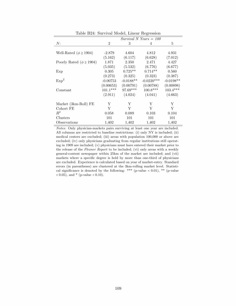
Table B24: Survival Model, Linear Regression

Survival N Years = 100N : 2 3 4 5

Well-Rated (φ ≥ 1904) -2.879 4.604 4.812 4.931(5.162) (6.117) (6.628) (7.012)

Poorly Rated (φ ≥ 1904) 1.871 2.350 2.471 4.427(5.035) (5.532) (6.776) (6.677)

Exp 0.305 0.725** 0.714** 0.560(0.273) (0.325) (0.323) (0.387)

Exp2 -0.00753 -0.0188** -0.0220*** -0.0198**(0.00653) (0.00791) (0.00788) (0.00898)

Constant 101.1*** 97.69*** 100.8*** 103.4***(2.911) (4.024) (4.041) (4.663)

Market (3km-Roll) FE Y Y Y YCohort FE Y Y Y YR2 0.058 0.089 0.103 0.104Clusters 101 101 101 101Observations 1,402 1,402 1,402 1,402

Notes: Only physician-markets pairs surviving at least one year are included.All columns are restricted to baseline restrictions: (i) only NY is included; (ii)medical centers are excluded; (iii) areas with population 100,000 or above areexcluded; (iv) only physicians graduating from regular institutions still operat-ing in 1909 are included; (v) physicians must have entered their market prior tothe release of the Flexner Report to be included; (vi) only areas with a weeklygeneral-content newspaper within 25km of the market are included; and (vii)markets where a specific degree is held by more than one-third of physiciansare excluded. Experience is calculated based on year of market-entry. Standarderrors (in parentheses) are clustered at the 3km-rolling market level. Statisti-cal significance is denoted by the following: *** (p-value < 0.01), ** (p-value< 0.05), and * (p-value < 0.10).

109

Table B25: Survival Model, Difference-in-Difference with Education Controls

Survival N Years = 100N : 2 3 4 5

Poorly Rated (φ ≥ 1904) 6.012 2.325 6.712 6.665(4.097) (4.720) (6.233) (6.644)

Poorly Rated (φ ∈ [1908,1909]) -14.10** -22.68** -31.08*** -25.43***(5.393) (9.487) (8.275) (9.332)

Exp 0.375 0.860** 0.924*** 0.711(0.278) (0.346) (0.338) (0.436)

Exp2 -0.00913 -0.0219** -0.0265*** -0.0226**(0.00692) (0.00842) (0.00812) (0.00974)

Constant 81.18*** 87.11*** 92.01*** 95.36***(18.60) (16.94) (18.23) (18.94)

Market (3km-Roll) FE Y Y Y YCohort FE Y Y Y YDegree FE Y Y Y YR2 0.110 0.136 0.149 0.141Clusters 101 101 101 101Observations 1,402 1,402 1,402 1,402

Notes: φ denotes entry year cohort for the physician-market pair. Only physician-marketspairs surviving at least one year are included. All columns are restricted to baselinerestrictions: (i) only NY is included; (ii) medical centers are excluded; (iii) areas withpopulation 100,000 or above are excluded; (iv) only physicians graduating from regularinstitutions still operating in 1909 are included; (v) physicians must have entered theirmarket prior to the release of the Flexner Report to be included; (vi) only areas witha weekly general-content newspaper within 25km of the market are included; and (vii)markets where a specific degree is held by more than one-third of physicians are excluded.Experience is calculated based on year of market-entry. Standard errors (in parentheses)are clustered at the 3km-rolling market level. Statistical significance is denoted by thefollowing: *** (p-value < 0.01), ** (p-value < 0.05), and * (p-value < 0.10).

110

Table B26: Survival, Bad News, Restricted to CME Rating A, Logit Model

Survival N Years = 100N : 2 3 4 5

‘Bad News’ 0.816* 0.612** 0.268 0.151(0.458) (0.242) (0.263) (0.252)

‘Bad News’ (φ ≥ 1904) 0.455 -0.0777 0.392 0.485(0.870) (0.468) (0.482) (0.489)

‘Bad News’ (φ ∈ [1908,1909]) -1.868** -2.064*** -2.306*** -2.088***(0.742) (0.716) (0.465) (0.452)

Exp 0.0466 0.0635** 0.0476* 0.0288(0.0409) (0.0274) (0.0255) (0.0290)

Exp2 -0.00145* -0.00188*** -0.00168*** -0.00126**(0.000834) (0.000529) (0.000507) (0.000559)

Constant 2.923*** 2.065*** 2.314*** 2.184***(0.526) (0.385) (0.332) (0.344)

Market (3km-Roll) FE Y Y Y YCohort FE Y Y Y YPseudo-R2 0.104 0.114 0.114 0.115Log Likelihood -187.7 -305.4 -371.3 -400.6Clusters 34 45 51 54Observations 727 818 860 880

Notes: Results presented are from logit models. Only physician-markets pairs surviving atleast one year are included. All columns are restricted to baseline restrictions: (i) only NY isincluded; (ii) medical centers are excluded; (iii) areas with population 100,000 or above areexcluded; (iv) only physicians graduating from regular institutions still operating in 1909 areincluded; (v) physicians must have entered their market prior to the release of the FlexnerReport to be included; (vi) only areas with a weekly general-content newspaper within 25kmof the market are included; and (vii) markets where a specific degree is held by more thanone-third of physicians are excluded. The sample is additionally restricted to physicians whoattended institutions directly rated A by the CME in 1910. Experience is calculated basedon year of market-entry. Standard errors (in parentheses) are clustered at the 3km-rollingmarket level. Statistical significance is denoted by the following: *** (p-value < 0.01), **(p-value < 0.05), and * (p-value < 0.10).

111

Table B27: Survival, 1908 and 1909 Separated

Survival N Years = 100N : 2 3 4 5

Poorly Rated 2.283 4.175** 2.537 2.760(1.570) (1.817) (2.368) (2.796)

Poorly Rated (φ ≥ 1904) 5.914 2.133 6.303 6.404(3.873) (5.186) (6.583) (6.600)

Poorly Rated (φ = 1908) -19.40** -27.06** -35.61*** -25.41*(7.932) (12.86) (12.93) (14.90)

Poorly Rated (φ = 1909) -7.672 -20.27* -28.83** -28.98**(6.210) (11.11) (12.08) (12.39)

Exp 0.344 0.683** 0.662* 0.521(0.272) (0.335) (0.342) (0.418)

Exp2 -0.00835 -0.0182** -0.0212** -0.0191**(0.00640) (0.00805) (0.00821) (0.00944)

Constant 100.9*** 99.18*** 103.0*** 105.2***(2.767) (3.649) (3.725) (4.441)

Market (3km-Roll) FE Y Y Y YCohort FE Y Y Y YR2 0.065 0.099 0.114 0.111Clusters 101 101 101 101Observations 1,402 1,402 1,402 1,402

Notes: φ denotes entry year cohort for the physician-market pair. Onlyphysician-markets pairs surviving at least one year are included. All columnsare restricted to baseline restrictions: (i) only NY is included; (ii) medical cen-ters are excluded; (iii) areas with population 100,000 or above are excluded; (iv)only physicians graduating from regular institutions still operating in 1909 areincluded; (v) physicians must have entered their market prior to the release ofthe Flexner Report to be included; (vi) only areas with a weekly general-contentnewspaper within 25km of the market are included; and (vii) markets where aspecific degree is held by more than one-third of physicians are excluded. Ex-perience is calculated based on year of market-entry. Standard errors (in paren-theses) are clustered at the 3km-rolling market level. Statistical significanceis denoted by the following: *** (p-value < 0.01), ** (p-value < 0.05), and *(p-value < 0.10).

112

Table B28: Survival Model by School Type, Linear Regression

Survival N Years = 100N : 2 3 4 5

Poorly-Rated Interacted With:Regular 2.626* 4.652*** 3.550 4.216

(1.436) (1.715) (2.218) (2.618)Regular (φ ≥ 1904) 6.521 1.784 5.425 5.698

(3.971) (5.566) (6.626) (6.580)Regular (φ ∈ [1908,1909]) -12.11** -21.84** -28.72*** -23.77***

(5.796) (10.08) (9.548) (8.355)Homeopathic 0.284 -1.150 -3.152 -2.364

(1.643) (3.065) (3.045) (3.392)Homeopathic (φ ≥ 1904) 12.54** 12.82* 16.25** 16.27**

(5.113) (7.264) (8.038) (7.847)Homeopathic (φ ∈ [1908,1909]) -12.62 -22.67** -27.32** -31.89**

(8.459) (11.30) (12.96) (14.61)Eclectic -0.0769 5.937 3.185 3.757

(4.517) (4.904) (6.579) (7.028)Eclectic (φ ≥ 1904) 11.82** 1.077 15.96 19.06

(5.158) (11.91) (13.70) (13.84)Eclectic (φ ∈ [1908,1909]) 1.425 7.004 1.164 0.729

(5.237) (11.71) (12.77) (12.79)Women-only 3.497*** -2.297 0.803 -7.667

(0.712) (11.33) (10.98) (11.33)Women-only (φ ≥ 1904) -7.748 5.818 7.980 21.11

(13.28) (16.50) (15.12) (16.66)Women-only (φ ∈ [1908,1909]) 16.28 13.61 15.35 18.93

(15.53) (17.17) (19.03) (19.32)No Interaction Terms:Exp 0.334 0.557** 0.442 0.541

(0.205) (0.252) (0.292) (0.351)

Exp2 -0.00816* -0.0150** -0.0149** -0.0200***(0.00475) (0.00575) (0.00637) (0.00720)

Constant 100.3*** 99.77*** 103.5*** 104.4***(2.179) (3.149) (3.388) (3.741)

Market (3km-Roll) FE Y Y Y YCohort FE Y Y Y YR2 0.062 0.084 0.091 0.097Clusters 101 101 101 101Observations 1,835 1,835 1,835 1,835

Notes: φ denotes entry year cohort for the physician-market pair. Only physician-marketspairs surviving at least one year are included. All columns are subject to the followingrestrictions: (i) only NY is included; (ii) medical centers are excluded; (iii) areas withpopulation 100,000 or above are excluded; (iv) physicians must have entered their marketprior to the release of the Flexner Report to be included; (v) only areas with a weeklygeneral-content newspaper within 25km of the market are included; and (vi) markets wherea specific degree is held by more than one-third of physicians are excluded. Experience iscalculated based on year of market-entry. Standard errors (in parentheses) are clusteredat the 3km-rolling market level. Statistical significance is denoted by the following: ***(p-value < 0.01), ** (p-value < 0.05), and * (p-value < 0.10).

113

Table B29: Survival, Falsification Test (1907-08)

Survival N Years = 100N : 2 3 4 5

Poorly Rated 2.078 3.943** 2.278 2.629(1.552) (1.821) (2.343) (2.749)

Poorly Rated (φ ≥ 1904) 4.946 -0.359 6.232 5.736(5.102) (6.548) (8.152) (7.355)

Poorly Rated (φ ∈ [1907,1908]) -6.516 -5.586 -15.36 -9.358(6.523) (8.607) (10.55) (9.109)

Exp 0.342 0.691** 0.796** 0.654(0.270) (0.341) (0.354) (0.406)

Exp2 -0.00814 -0.0183** -0.0239*** -0.0216**(0.00649) (0.00833) (0.00839) (0.00933)

Constant 100.6*** 98.66*** 101.8*** 103.8***(2.766) (3.826) (3.867) (4.469)

Market (3km-Roll) FE Y Y Y YCohort FE Y Y Y YR2 0.065 0.093 0.105 0.106Clusters 101 101 101 101Observations 1,340 1,340 1,340 1,340

Notes: φ denotes entry year cohort for the physician-market pair. Only physician-marketspairs surviving at least one year are included. All columns are restricted to baselinerestrictions: (i) only NY is included; (ii) medical centers are excluded; (iii) areas withpopulation 100,000 or above are excluded; (iv) only physicians graduating from regularinstitutions still operating in 1908 are included; (v) physicians must have entered theirmarket prior to the release of the Flexner Report to be included; (vi) only areas witha weekly general-content newspaper within 25km of the market are included; and (vii)markets where a specific degree is held by more than one-third of physicians are excluded.Experience is calculated based on year of market-entry. Standard errors (in parentheses)are clustered at the 3km-rolling market level. Statistical significance is denoted by thefollowing: *** (p-value < 0.01), ** (p-value < 0.05), and * (p-value < 0.10).

114

Table B30: Survival, Falsification Test (1906-07)

Survival N Years = 100N : 2 3 4 5

Poorly Rated 1.945 3.928** 2.326 2.770(1.537) (1.795) (2.325) (2.721)

Poorly Rated (φ ≥ 1904) 7.070 2.333 6.747 8.267(5.773) (6.474) (6.624) (6.234)

Poorly Rated (φ ∈ [1906,1907]) -1.519 -0.0394 -0.413 -3.138(7.678) (7.536) (8.757) (9.865)

Exp 0.377 0.648* 0.734** 0.662(0.283) (0.361) (0.370) (0.421)

Exp2 -0.00877 -0.0177** -0.0229*** -0.0215**(0.00668) (0.00867) (0.00865) (0.00959)

Constant 100.5*** 99.53*** 102.5*** 103.8***(2.786) (3.852) (4.034) (4.308)

Market (3km-Roll) FE Y Y Y YCohort FE Y Y Y YR2 0.071 0.097 0.111 0.112Clusters 101 101 101 101Observations 1,283 1,283 1,283 1,283

Notes: φ denotes entry year cohort for the physician-market pair. Only physician-marketspairs surviving at least one year are included. All columns are restricted to baselinerestrictions: (i) only NY is included; (ii) medical centers are excluded; (iii) areas withpopulation 100,000 or above are excluded; (iv) only physicians graduating from regularinstitutions still operating in 1907 are included; (v) physicians must have entered theirmarket prior to the release of the Flexner Report to be included; (vi) only areas witha weekly general-content newspaper within 25km of the market are included; and (vii)markets where a specific degree is held by more than one-third of physicians are excluded.Experience is calculated based on year of market-entry. Standard errors (in parentheses)are clustered at the 3km-rolling market level. Statistical significance is denoted by thefollowing: *** (p-value < 0.01), ** (p-value < 0.05), and * (p-value < 0.10).

115

Table B31: LPM, Bad News v. Poor CME Rating, Difference-in-Difference

Survival N Years = 100N : 2 3 4 5

‘Bad News’ 2.579* 4.470*** 2.766 2.964(1.452) (1.682) (2.250) (2.675)

‘Bad News’ (φ ≥ 1904) 5.548 2.478 6.672 6.702(3.874) (5.146) (6.560) (6.579)

‘Bad News’ (φ ∈ [1908,1909]) -14.35** -23.96** -33.14*** -28.02***(5.600) (9.133) (8.149) (8.075)

CME: Rated B/C -9.115 -6.875 -6.394 -4.851(11.00) (11.49) (11.67) (11.77)

CME: Rated B/C (φ ≥ 1904) 17.03 -27.90 -23.72 -16.51(11.15) (36.73) (36.26) (39.79)

CME: Rated B/C (φ ∈ [1908,1909]) 1.349 12.07 11.39 7.724(4.920) (44.31) (44.59) (48.12)

Exp 0.368 0.685** 0.667* 0.513(0.273) (0.330) (0.337) (0.412)

Exp2 -0.00881 -0.0183** -0.0214*** -0.0191**(0.00644) (0.00794) (0.00809) (0.00928)

Constant 100.7*** 99.15*** 102.9*** 105.2***(2.772) (3.697) (3.805) (4.563)

Market (3km-Roll) FE Y Y Y YCohort FE Y Y Y YR2 0.066 0.101 0.115 0.112Clusters 101 101 101 101Observations 1,402 1,402 1,402 1,402

Notes: φ denotes entry year cohort for the physician-market pair. Only physician-marketspairs surviving at least one year are included. All columns are restricted to baseline restric-tions: (i) only NY is included; (ii) medical centers are excluded; (iii) areas with population100,000 or above are excluded; (iv) only physicians graduating from regular institutions stilloperating in 1909 are included; (v) physicians must have entered their market prior to therelease of the Flexner Report to be included; (vi) only areas with a weekly general-contentnewspaper within 25km of the market are included; and (vii) markets where a specific degreeis held by more than one-third of physicians are excluded. Experience is calculated based onyear of market-entry. Standard errors (in parentheses) are clustered at the 3km-rolling marketlevel. Statistical significance is denoted by the following: *** (p-value < 0.01), ** (p-value< 0.05), and * (p-value < 0.10).

116

Table B32: Survival, Logit Model

Survival N Years = 100N : 2 3 4 5

Poorly-Rated 0.620 0.536** 0.270 0.237(0.461) (0.223) (0.226) (0.231)

Poorly-Rated (φ ≥ 1904) 0.600 -0.0292 0.296 0.289(0.776) (0.451) (0.442) (0.418)

Poorly-Rated (φ ∈ [1908,1909]) -1.855** -2.102*** -2.090*** -1.562***(0.737) (0.723) (0.485) (0.454)

Exp 0.0623 0.0607** 0.0464** 0.0298(0.0403) (0.0248) (0.0226) (0.0263)

Exp2 -0.00149* -0.00157*** -0.00148*** -0.00116**(0.000869) (0.000513) (0.000480) (0.000533)

Constant 2.928*** 1.992*** 2.223*** 2.008***(0.429) (0.304) (0.262) (0.308)

Market (3km-Roll) FE Y Y Y YCohort FE Y Y Y YPseudo-R2 0.081 0.086 0.086 0.080Log Likelihood -261.9 -442.4 -526.7 -581.9Clusters 39 51 57 62Observations 1,078 1,174 1,207 1,239

Notes: Results presented are from logit models. Only physician-markets pairs surviving atleast one year are included. All columns are restricted to baseline restrictions: (i) only NYis included; (ii) medical centers are excluded; (iii) areas with population 100,000 or above areexcluded; (iv) only physicians graduating from regular institutions still operating in 1909 areincluded; (v) physicians must have entered their market prior to the release of the FlexnerReport to be included; (vi) only areas with a weekly general-content newspaper within 25kmof the market are included; and (vii) markets where a specific degree is held by more thanone-third of physicians are excluded. Standard errors (in parentheses) are clustered at the 3km-rolling market level. Statistical significance is denoted by the following: *** (p-value < 0.01),** (p-value < 0.05), and * (p-value < 0.10).

117

Table B33: Survival, Bad News, Logit Model

Survival N Years = 100N : 2 3 4 5

‘Bad News’ 0.751* 0.584*** 0.299 0.258(0.415) (0.199) (0.206) (0.212)

‘Bad News’ (φ ≥ 1904) 0.466 0.00840 0.330 0.311(0.750) (0.448) (0.437) (0.411)

‘Bad News’ (φ ∈ [1908,1909]) -2.041*** -1.993*** -2.085*** -1.574***(0.763) (0.628) (0.461) (0.412)

Exp 0.0637 0.0615** 0.0472** 0.0303(0.0403) (0.0247) (0.0224) (0.0263)

Exp2 -0.00153* -0.00159*** -0.00150*** -0.00117**(0.000870) (0.000510) (0.000477) (0.000531)

Constant 2.894*** 2.000*** 2.227*** 2.010***(0.427) (0.297) (0.258) (0.304)

Market (3km-Roll) FE Y Y Y YCohort FE Y Y Y YPseudo-R2 0.084 0.086 0.086 0.080Log Likelihood -261.1 -442.4 -526.6 -581.7Clusters 39 51 57 62Observations 1,078 1,174 1,207 1,239

Notes: Results presented are from logit models. Only physician-markets pairs surviving atleast one year are included. All columns are restricted to baseline restrictions: (i) only NY isincluded; (ii) medical centers are excluded; (iii) areas with population 100,000 or above areexcluded; (iv) only physicians graduating from regular institutions still operating in 1909 areincluded; (v) physicians must have entered their market prior to the release of the FlexnerReport to be included; (vi) only areas with a weekly general-content newspaper within 25kmof the market are included; and (vii) markets where a specific degree is held by more thanone-third of physicians are excluded. Standard errors (in parentheses) are clustered at the3km-rolling market level. Statistical significance is denoted by the following: *** (p-value< 0.01), ** (p-value < 0.05), and * (p-value < 0.10).

118

Table B34: Survival, Probit Model

Survival N Years = 100N : 2 3 4 5

Poorly-Rated 0.286 0.281** 0.132 0.126(0.230) (0.124) (0.129) (0.134)

Poorly-Rated (φ ≥ 1904) 0.305 -0.0123 0.190 0.190(0.383) (0.247) (0.249) (0.239)

Poorly-Rated (φ ∈ [1908,1909]) -0.903** -1.129*** -1.207*** -0.923***(0.365) (0.400) (0.283) (0.265)

Exp 0.0298 0.0315** 0.0245* 0.0162(0.0197) (0.0141) (0.0132) (0.0155)

Exp2 -0.000719* -0.000827*** -0.000807*** -0.000652**(0.000430) (0.000301) (0.000287) (0.000320)

Constant 1.640*** 1.183*** 1.312*** 1.193***(0.217) (0.174) (0.152) (0.179)

Market (3km-Roll) FE Y Y Y YCohort FE Y Y Y YPseudo-R2 0.080 0.084 0.085 0.080Log Likelihood -262.3 -443.0 -527.1 -582.0Clusters 39 51 57 62Observations 1,078 1,174 1,207 1,239

Notes: Results presented are from probit models. Only physician-markets pairs surviving at leastone year are included. All columns are restricted to baseline restrictions: (i) only NY is included;(ii) medical centers are excluded; (iii) areas with population 100,000 or above are excluded; (iv) onlyphysicians graduating from regular institutions still operating in 1909 are included; (v) physiciansmust have entered their market prior to the release of the Flexner Report to be included; (vi) onlyareas with a weekly general-content newspaper within 25km of the market are included; and (vii)markets where a specific degree is held by more than one-third of physicians are excluded. Standarderrors (in parentheses) are clustered at the 3km-rolling market level. Statistical significance isdenoted by the following: *** (p-value < 0.01), ** (p-value < 0.05), and * (p-value < 0.10).

119

Table B35: Survival by School Type, Logit Model

Survival N Years = 100N : 2 3 4 5

Poorly-Rated Interacted With:Regular 0.696* 0.540*** 0.329 0.344*

(0.416) (0.205) (0.200) (0.206)Regular (φ ≥ 1904) 0.607 -0.0644 0.174 0.155

(0.799) (0.472) (0.430) (0.397)Regular (φ ∈ [1908,1909]) -1.661** -1.858** -1.794*** -1.363***

(0.751) (0.735) (0.556) (0.414)Homeopathic 0.138 -0.131 -0.249 -0.179

(0.384) (0.286) (0.225) (0.221)Homeopathic (φ ≥ 1904) 2.107 1.196* 1.145** 1.046**

(1.290) (0.705) (0.568) (0.521)Homeopathic (φ ∈ [1908,1909]) -2.240* -2.195** -1.866** -1.885***

(1.359) (0.902) (0.774) (0.717)No Interaction Terms:Exp 0.0587** 0.0497** 0.0302 0.0293

(0.0297) (0.0197) (0.0189) (0.0213)

Exp2 -0.00138** -0.00131*** -0.00100*** -0.00111***(0.000625) (0.000393) (0.000374) (0.000404)

Constant 2.740*** 1.951*** 2.056*** 1.789***(0.336) (0.234) (0.204) (0.207)

Market (3km-Roll) FE Y Y Y YCohort FE Y Y Y YPseudo-R2 0.082 0.076 0.069 0.074Log Likelihood -354.0 -607.2 -739.0 -817.1Clusters 47 62 69 75Observations 1,466 1,613 1,656 1,714

Notes: Results presented are from logit models. φ denotes entry year cohort for the physician-market pair. Only physician-markets pairs surviving at least one year are included. All columnsare subject to the following restrictions: (i) only NY is included; (ii) medical centers are excluded;(iii) areas with population 100,000 or above are excluded; (iv) physicians must have enteredtheir market prior to the release of the Flexner Report to be included; (v) only areas with aweekly general-content newspaper within 25km of the market are included; and (vi) marketswhere a specific degree is held by more than one-third of physicians are excluded. Experienceis calculated based on year of market-entry. Standard errors (in parentheses) are clustered atthe 3km-rolling market level. Statistical significance is denoted by the following: *** (p-value< 0.01), ** (p-value < 0.05), and * (p-value < 0.10).

120

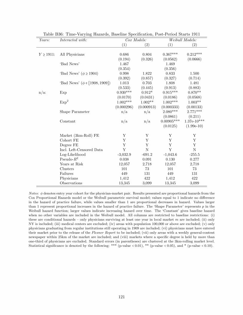
Table B36: Time-Varying Hazards, Baseline Specification, Post-Period Starts 1911

Years: Interacted with: Cox Models: Weibull Models:(1) (2) (1) (2)

Y ≥ 1911: All Physicians 0.686 0.804 0.367*** 0.212***(0.194) (0.326) (0.0562) (0.0666)

‘Bad News’ 1.467 1.469(0.354) (0.356)

‘Bad News’ (φ ≥ 1904) 0.998 1.822 0.833 1.500(0.392) (0.857) (0.327) (0.714)

‘Bad News’ (φ ∈ [1908,1909]) 1.013 0.703 1.808 1.481(0.533) (0.445) (0.913) (0.883)

n/a: Exp 0.930*** 0.912* 0.915*** 0.870**(0.0170) (0.0431) (0.0186) (0.0568)

Exp2 1.002*** 1.002** 1.002*** 1.003**(0.000296) (0.000913) (0.000333) (0.00133)

Shape Parameter n/a n/a 2.080*** 2.771***(0.0861) (0.211)

Constant n/a n/a 0.00905*** 1.37e-10***(0.0125) (1.99e-10)

Market (3km-Roll) FE Y Y Y YCohort FE Y Y Y YDegree FE Y Y Y YIncl. Left-Censored Data Y N Y NLog-Likelihood -3,032.9 -691.2 -1,043.6 -255.5Pseudo-R2 0.038 0.091 0.130 0.277Years at Risk 12,057 2,718 12,057 2,718Clusters 101 73 101 73Failures 449 131 449 131Physicians 1,412 422 1,412 422Observations 13,345 3,099 13,345 3,099

Notes: φ denotes entry year cohort for the physician-market pair. Results presented are proportional hazards from theCox Proportional Hazards model or the Weibull parametric survival model; values equal to 1 indicate no differencein the hazard of practice failure, while values smaller than 1 are proportional decreases in hazard. Values largerthan 1 represent proportional increases in the hazard of practice failure. The ‘Shape Parameter’ represents p in theWeibull hazard function; larger values indicate increasing hazard over time. The ‘Constant’ gives baseline hazardwhen no other variables are included in the Weibull model. All columns are restricted to baseline restrictions: (i)these are conditional hazards – only physicians surviving at least one year in local market m are included; (ii) onlyNY is included; (iii) medical centers are excluded; (iv) areas with population 100,000 or above are excluded; (v) onlyphysicians graduating from regular institutions still operating in 1909 are included; (vi) physicians must have enteredtheir market prior to the release of the Flexner Report to be included; (vii) only areas with a weekly general-contentnewspaper within 25km of the market are included; and (viii) markets where a specific degree is held by more thanone-third of physicians are excluded. Standard errors (in parentheses) are clustered at the 3km-rolling market level.Statistical significance is denoted by the following: *** (p-value < 0.01), ** (p-value < 0.05), and * (p-value < 0.10).

121

Table B37: Single-Year Survival, By Degree Share, LPM

Survival to Year Y = 1 1

No High-Quality Competitor RestrictionMax. Share 1909-10 1910-11 1911-12 1912-13 1913-14

≤ 25% -0.180** 0.0176 -0.174* 0.0527 0.00828(0.0834) (0.0818) (0.0887) (0.123) (0.0210)

≤ 33.3% -0.169** 0.0173 -0.131** -0.0132 0.0534(0.0685) (0.0670) (0.0517) (0.0667) (0.0597)

< 50% -0.123** 0.0110 -0.0271 -0.0954* 0.0538(0.0482) (0.0531) (0.0533) (0.0535) (0.0439)

≤ 50% -0.127*** -0.000386 -0.0318 -0.0257 0.0518(0.0465) (0.0492) (0.0485) (0.0504) (0.0424)

< 100% -0.0851** -0.0234 -0.00611 -0.0142 0.0372(0.0404) (0.0410) (0.0434) (0.0400) (0.0350)

Any Share -0.0842** -0.0217 -0.00672 -0.0211 0.0221(0.0397) (0.0408) (0.0427) (0.0394) (0.0353)

Restricted to Areas with High-Quality Competition2

Max. Share 1909-10 1910-11 1911-12 1912-13 1913-14

≤ 25% -0.184** 0.0205 -0.180* 0.0542 0.00893(0.0840) (0.0827) (0.0909) (0.126) (0.0214)

≤ 33.3% -0.171** 0.0169 -0.134** -0.0139 0.0534(0.0687) (0.0673) (0.0526) (0.0677) (0.0609)

< 50% -0.133*** 0.00958 -0.0448 -0.0939* 0.0549(0.0486) (0.0547) (0.0533) (0.0543) (0.0448)

≤ 50% -0.127*** -0.00193 -0.0448 -0.0457 0.0416(0.0471) (0.0516) (0.0490) (0.0502) (0.0428)

< 100% -0.0967** -0.0154 -0.00899 -0.0392 0.0313(0.0414) (0.0439) (0.0440) (0.0417) (0.0360)

Any Share -0.104** -0.0126 -0.00994 -0.0472 0.0265(0.0413) (0.0443) (0.0433) (0.0418) (0.0359)

Notes: [1] Dependent variable is survival to end year, conditional on survivalto start year. [2] The bottom panel is restricted to markets where a well-ratedphysician was present in some year 1903-1909. [3] Coefficients correspond with‘Bad News’ (φ ∈ [1908,1909]) in a linear probability model, where φ denotesentry year cohort for the physician-market pair. All estimates are restrictedto the following restrictions: (i) only NY is included; (ii) medical centersare excluded; (iii) areas with population 100,000 or above are excluded; (iv)only physicians graduating from regular institutions still operating in 1909are included; and (v) physicians must have entered their market prior to therelease of the Flexner Report to be included. Standard errors (in parentheses)are clustered at the 3km-rolling market level. Statistical significance is denotedby the following: *** (p-value < 0.01), ** (p-value < 0.05), and * (p-value< 0.10).

122

Table B38: Cox Model, Well-Rated Physicians

(1) (2) (3) (4) (5)

Well-Rated 0.974(0.114)

Well-Rated (φ ≥ 1904) 1.365(0.372)

Well-Rated (φ ∈ [1908,1909]) 0.346***(0.122)

Well-Rated & CME: A 0.950(0.116)

Well-Rated & CME: A (φ ≥ 1904) 1.365(0.372)

Well-Rated & CME: A (φ ∈ [1908,1909]) 0.346*** 0.336**(0.122) (0.156)

Exp 0.998 0.998 0.999 0.999 1.014(0.0147) (0.0145) (0.0147) (0.0147) (0.0370)

Exp2 1.001*** 1.001*** 1.001** 1.001** 1.000(0.000274) (0.000268) (0.000279) (0.000279) (0.000829)

Market (3km-Roll) FE Y Y Y Y YCohort FE Y Y Y Y YDegree FE N N Y Y YIncl. Left-Censored Data Y Y Y Y NLog-Likelihood -3,073.1 -3,073.0 -3,048.4 -3,048.4 -692.8Pseudo-R2 0.029 0.029 0.037 0.037 0.089Years at Risk 12,077 12,077 12,077 12,077 2,718Clusters 101 101 101 101 73Failures 451 451 451 451 131Observations 1,414 1,414 1,414 1,414 422

Notes: φ denotes entry year cohort for the physician-market pair. Results presented are proportional hazards fromthe Cox Proportional Hazards model; values equal to 1 indicate no difference in the hazard of practice failure, whilevalues smaller than 1 are proportional decreases in hazard. Values larger than 1 represent proportional increases inthe hazard of practice failure. All columns are restricted to baseline restrictions: (i) these are conditional hazards– only physicians surviving at least one year in local market m are included; (ii) only NY is included; (iii) medicalcenters are excluded; (iv) areas with population 100,000 or above are excluded; (v) only physicians graduating fromregular institutions still operating in 1909 are included; (vi) physicians must have entered their market prior to therelease of the Flexner Report to be included; (vii) only areas with a weekly general-content newspaper within 25kmof the market are included; and (viii) markets where a specific degree is held by more than one-third of physiciansare excluded. Standard errors (in parentheses) are clustered at the 3km-rolling market level. Statistical significanceis denoted by the following: *** (p-value < 0.01), ** (p-value < 0.05), and * (p-value < 0.10).

123

Table B39: Time-Varying Hazards, Well-Rated Physicians, Post-Period Interactions

Years: Interacted with: Cox Models: Weibull Models:(1) (2) (1) (2)

Y ≥ 1910: All Physicians 1.015 0.683 0.429*** 0.235***(0.290) (0.299) (0.0589) (0.0914)

Well-Rated 1.058 1.044(0.269) (0.270)

Well-Rated (φ ≥ 1904) 0.930 1.535 0.979 1.447(0.286) (0.821) (0.301) (0.664)

Well-Rated (φ ∈ [1908,1909]) 0.428* 0.274** 0.412** 0.272**(0.187) (0.165) (0.183) (0.164)

n/a: Exp 0.996 1.013 0.992 1.011(0.0145) (0.0370) (0.0158) (0.0431)

Exp2 1.001*** 1.000 1.001*** 1.000(0.000278) (0.000829) (0.000323) (0.00104)

Shape Parameter n/a n/a 2.077*** 2.428***(0.0715) (0.204)

Constant n/a n/a 0.00413*** 6.81e-11***(0.00558) (9.74e-11)

Market (3km-Roll) FE Y Y Y YCohort FE Y Y Y YDegree FE Y Y Y YIncl. Left-Censored Data Y N Y NLog-Likelihood -3,034.3 -692.2 -1,048.1 -264.4Pseudo-R2 0.037 0.090 0.126 0.252Years at Risk 12,057 2,718 12,057 2,718Clusters 101 73 101 73Failures 449 131 449 131Physicians 1,412 422 1,412 422Observations 13,345 3,099 13,345 3,099

Notes: φ denotes entry year cohort for the physician-market pair. Results presented are proportionalhazards from the Cox Proportional Hazards model or the Weibull parametric survival model; values equalto 1 indicate no difference in the hazard of practice failure, while values smaller than 1 are proportionaldecreases in hazard. Values larger than 1 represent proportional increases in the hazard of practice failure.The ‘Shape Parameter’ represents p in the Weibull hazard function; larger values indicate increasinghazard over time. The ‘Constant’ gives baseline hazard when no other variables are included in theWeibull model. All columns are restricted to baseline restrictions: (i) these are conditional hazards –only physicians surviving at least one year in local market m are included; (ii) only NY is included; (iii)medical centers are excluded; (iv) areas with population 100,000 or above are excluded; (v) only physiciansgraduating from regular institutions still operating in 1909 are included; (vi) physicians must have enteredtheir market prior to the release of the Flexner Report to be included; (vii) only areas with a weeklygeneral-content newspaper within 25km of the market are included; and (viii) markets where a specificdegree is held by more than one-third of physicians are excluded. Standard errors (in parentheses) areclustered at the 3km-rolling market level. Statistical significance is denoted by the following: *** (p-value< 0.01), ** (p-value < 0.05), and * (p-value < 0.10).

124

Table B40: Survival Analysis, By School Type

Cox Models: Weibull Models:(1) (2) (3) (1) (2) (3)

Poorly-Rated Interaction:Regular 0.938 0.937

(0.111) (0.116)Regular (φ ≥ 1904) 0.876 0.837 0.794 0.863 0.824 0.756

(0.241) (0.227) (0.250) (0.255) (0.237) (0.264)Regular (φ ∈ [1908,1909]) 2.614*** 2.593** 2.445** 2.807*** 2.716** 2.645**

(0.967) (0.960) (1.033) (1.120) (1.054) (1.229)Homeo. 1.212 1.225

(0.167) (0.177)Homeo. (φ ≥ 1904) 0.614 0.764 0.844 0.582 0.750 0.849

(0.241) (0.283) (0.258) (0.241) (0.289) (0.287)Homeo. (φ ∈ [1908,1909]) 2.508** 2.025 2.076 2.645** 2.065 2.053

(1.156) (0.906) (1.076) (1.302) (0.960) (1.159)No Interaction Terms:Exp 0.992 0.988 1.000 0.988 0.985 0.995

(0.0111) (0.0114) (0.0229) (0.0119) (0.0120) (0.0266)

Exp2 1.001*** 1.001*** 1.000 1.001*** 1.001*** 1.001(0.000207) (0.000206) (0.000490) (0.000230) (0.000224) (0.000594)

Shape Parameter n/a n/a n/a

Constant n/a n/a n/a

Market (3km-Roll) FE Y Y Y Y Y YCohort FE Y Y Y Y Y YDegree FE Y N N Y N NIncl. Left-Censored Data Y Y N Y Y NLog-Likelihood -4,417.9 -4,462.3 -1,021.4 -1,440.6 -1,490.2 -403.0Pseudo-R2 0.035 0.025 0.043 0.114 0.083 0.122Years at Risk 15,625 15,625 3,445 15,625 15,625 3,445Clusters 101 101 77 101 101 77Failures 629 629 177 629 629 177Observations 1,847 1,847 537 1,847 1,847 537

Notes: In this table, all variables listing ‘Regular’ and ‘Homeo.’ physicians were those rated poorly by Flexner.‘Homeo.’ is an abbreviation for ‘Homeopathic.’ φ denotes entry year cohort for the physician-market pair. Resultspresented are proportional hazards from the Cox Proportional Hazards model or the Weibull parametric survivalmodel; values equal to 1 indicate no difference in the hazard of practice failure, while values smaller than 1 areproportional decreases in hazard. Values larger than 1 represent proportional increases in the hazard of practicefailure. The ‘Shape Parameter’ represents p in the Weibull hazard function; larger values indicate increasing hazardover time. The ‘Constant’ gives baseline hazard when no other variables are included in the Weibull model. Allcolumns are restricted to the following: (i) these are conditional hazards – only physicians surviving at least oneyear in local market m are included; (ii) only NY is included; (iii) medical centers are excluded; (iv) areas withpopulation 100,000 or above are excluded; (v) physicians must have entered their market prior to the release of theFlexner Report to be included; (vi) only areas with a weekly general-content newspaper within 25km of the marketare included; and (vii) markets where a specific degree is held by more than one-third of physicians are excluded.Standard errors (in parentheses) are clustered at the 3km-rolling market level. Statistical significance is denoted bythe following: *** (p-value < 0.01), ** (p-value < 0.05), and * (p-value < 0.10).

125

Table B41: Sorting: Changing Practice Locations, New York

From Rural From Urban Population Change Urban to UrbanRural Urban Rural Urban Total ↑ ↓ ↑ ↓

1904 24 39 12 45 120 61 35 22 231905 12 41 19 50 122 73 37 32 181906 18 39 23 65 145 76 51 37 281907 17 45 23 86 171 98 56 53 331908 21 43 30 61 155 71 63 28 331909 23 46 29 71 169 85 61 39 321910 16 35 27 70 148 79 53 44 261911 24 50 34 86 194 99 71 49 371912 24 54 31 79 188 96 68 42 371913 15 47 34 72 168 89 64 42 301914 12 39 23 80 154 88 54 49 31

Total: 206 478 285 765 1,734 915 613 437 328

1904-09 (%): 13.0 28.7 15.4 42.9 100.0 52.6 34.4 23.9 18.91910-14 (%): 10.7 26.4 17.5 45.4 100.0 52.9 36.4 26.5 18.9

Overall (%): 11.9 27.6 16.4 44.1 100.0 52.8 35.4 25.2 18.9

Notes: Data are restricted to physicians who relocate to New York from some initial market. Yearsrefer to the date of relocation. Comparison data for locations are from the last post-office the physicianwas listed under in their previous 3km-rolling market. Urban areas are defined as incorporated areasin the 1910 federal census; all other areas are listed as rural. The right panel counts the number ofphysicians who moved to areas with higher or lower total population than their former post-officelocation, with the two rightmost columns restricting to physicians moving between two incorporatedplaces. In both samples, physicians relocate more often to areas with higher populations than to areaswith lower populations, both in the pre-period and the post-period.

126

Table B42: Physician Location Choice, New York

Binary Outcome: Entered Urban AreaUrb1 Urb5 Urb10 Urb25

Exp -0.00719 -0.00729 -0.00993 -0.00919(0.00844) (0.00763) (0.00836) (0.00822)

Exp2 -7.23e-05 -0.000172 -0.000169 -0.000189(0.000154) (0.000130) (0.000147) (0.000158)

Trend 0.00380 0.00285 0.0161 0.0292(0.0244) (0.0212) (0.0256) (0.0335)

Trend: Bad News 0.0240 0.0254 0.0150 0.0243(0.0420) (0.0353) (0.0381) (0.0378)

Trend: Well-Rated -0.0138 -0.0264 -0.0330 -0.0110(0.0277) (0.0284) (0.0308) (0.0401)

Post 0.256 0.405** 0.373** 0.432(0.213) (0.160) (0.176) (0.271)

Post*Bad News -0.357 -0.405** -0.354* -0.542*(0.272) (0.199) (0.208) (0.282)

Post*Well-Rated -0.0409 -0.167 -0.107 -0.398(0.278) (0.318) (0.300) (0.423)

Fresh Entry 0.416** 0.438** 0.491*** 0.716***(0.199) (0.179) (0.181) (0.179)

Fresh*Bad News 0.0935 0.313 0.349 0.208(0.257) (0.266) (0.273) (0.325)

Fresh*Well-Rated 0.294 0.216 0.170 0.0732(0.234) (0.267) (0.261) (0.301)

Post*Fresh -0.146 -0.205 -0.240 -0.416*(0.179) (0.294) (0.250) (0.217)

Post*Fresh*Bad News 0.328 0.233 0.206 0.364(0.224) (0.316) (0.282) (0.262)

Post*Fresh*Well-Rated -0.216 -0.00651 -0.0249 0.0759(0.249) (0.329) (0.282) (0.274)

Constant -5.365 -4.024 -29.42 -55.01(46.53) (40.38) (48.89) (63.94)

Degree FE Y Y Y YLog-Likelihood -6,171.1 -7,114.8 -7,137.0 -6,887.0

Pseudo-R2 0.038 0.044 0.046 0.053Clusters 83 86 87 89

Observations 10,768 10,790 10,792 10,800

Notes: Results presented are from logit models. Outcome variables denote whethera physician’s post-office location choice is an urban area, where urban area is de-fined by a population equal to or exceeding m-thousand for the variable Urbm.Populations are for incorporated areas in the 1910 federal census. All columns arerestricted to physicians locating to the state of New York and include degree fixedeffects. Standard errors (in parentheses) are clustered at the degree level. Statisticalsignificance is denoted by the following: *** (p-value < 0.01), ** (p-value < 0.05),and * (p-value < 0.10).

127

Table B43: Dishonesty in Education Reporting, New York

Ambiguous or Misleading Education String(1) (2) (3) (4)

Trend -0.0904*** -0.102***(0.0235) (0.0242)

Trend: Bad News 0.870** 0.964** 0.644*** 0.714***(0.422) (0.449) (0.152) (0.152)

Trend: Well-Rated 0.276 0.308 0.285 0.317(0.272) (0.290) (0.185) (0.197)

Post 0.219** 0.199***(0.0867) (0.0750)

Post*Bad News -3.881** -4.122** -2.925*** -2.998***(1.746) (1.947) (0.453) (0.509)

Post*Well-Rated -1.276 -1.520 -1.409** -1.655**(0.986) (1.021) (0.679) (0.701)

Constant 169.1*** 192.2*** -5.514*** -5.024**(44.81) (45.89) (1.917) (2.006)

Incl. Post-Period Entrants Y N Y NCohort FE Y Y Y Y

Year FE N N Y YDegree FE Y Y Y Y

Market (3km-roll) FE Y Y Y YLog-Likelihood -4,838.7 -4,324.6 -4,353.1 -3,862.0

Pseudo-R2 0.796 0.796 0.816 0.818Clusters 58 54 58 54

Observations 39,921 35,195 39,921 35,195

Notes: Results presented are from logit models. Sample area is New York state ex-cluding medical centers and post-offices with populations of 100k or more. Experienceand its square are included as control variables; neither variable is significant in anymodel. Standard errors (in parentheses) are clustered at the degree level. Statisticalsignificance is denoted by the following: *** (p-value < 0.01), ** (p-value < 0.05), and* (p-value < 0.10).

128

Table B44: Consumer Spending per Physician, USA, 1909-1919

1909 1914 1919Population (000s) 90,490 99,111 104,514

Per Capita Annual ExpenditurePhysicians $3.24 $2.99 $6.87Dentists $0.91 $0.95 $2.65Food $81.43 $90.34 $177.53Consumer Expenditures $318.42 $336.95 $579.57

Estimates for USA EconomyPhysician Expenditures $293,187,600 $296,341,890 $718,011,180# Physicians (AMD) 133,487 142,332 147,0741

Mean Physician Income $2,196.38 $2,082.05 $4,881.98# Phys (Polk) 137,4312 132,760Mean Physician Income $2,133.34 $2,232.16

Sources:

[a] Population: Census Bureau Statistical Abstract of the US for 1921.

[b] Expenditures: Derks (1999)

[c] Bottom Panel: author calculations.

Notes: [1] Count is for 1918. [2] Count is for 1908.

129

Appendix C: Connecticut and New Jersey

Figure A6 provided compelling visual evidence that the Flexner Report had an impact on the

survival of physician practices in the state of New York. I find mixed evidence of this impact in

New Jersey and no evidence for it in Connecticut. Figures C1 and C2 plot corresponding survival

curves for New Jersey and Connecticut physicians, respectively.168

Figure C1: Survival by Rating and Cohort, New Jersey, 1907-09

In Jersey, there appears to be no impact on the 1909 cohort and a minimal effect that was not

sustained on the 1908 cohort. The 1907 cohort sees an immediate improvement in the survival of

the well-rated physicians in 1908 relative to the poorly rated – well before the introduction of the

Flexner Report. In Connecticut, the survival curves exhibit a lot of noise, especially for the 1909

cohort. Although it does show a substantial gap for this cohort, no failures are recorded between

1911 and 1914. The 1907 and and 1908 cohorts also do not behave as expected.

168As it is a medical center, New Haven is excluded from the the Connecticut analysis.

130

Figure C2: Survival by Rating and Cohort, Connecticut, 1907-09

While the results in Connecticut could be explained by the smaller population of physicians in

the state, and explanation could be posited for the patterns observed in New Jersey, there are hints

of a more pernicious systematic problem in the data for these states. Table C1 lists the number

of market entries for each cohort by state.169 Outlier years are immediately noticeable for both

Connecticut and New Jersey, but not New York. In Connecticut, many entries were recorded in

1904, 1908, and 1910, but very few were recorded in 1906 or 1909. In New Jersey, many entries

were recorded in 1904, 1905, and 1913 but very few were recorded in 1906, 1910, or 1912. This

bunching hints at a recording problem in the original directories: updates for Connecticut and New

Jersey may have been made only sporadically.

169See Figure A12 for a chart with these data plotted for 1904-1914.

131

Table C1: Market Entries (3km, Rolling)Year CT NJ NY

≤1903 1,181 1,996 5,8111904 164 260 5161905 73 226 3851906 31 98 5451907 79 134 4761908 140 193 4461909 20 186 5211910 108 94 4281911 60 157 4771912 42 83 4211913 72 218 3721914 72 110 448

Panel 2,042 3,755 10,846

Figure C3 plots the percentage of total market entries in a state over the period 1904-1914

by year, with a horizontal line denoting an equal number of entries per year. The takeaway is

stark: New York data has a similar percentage of entries recorded every year whereas the plots for

Connecticut and New Jersey are erratic. It is clear that new entries are not necessarily recorded in

each year outside New York. Given this failure in the underlying data generating process, I inspect

next whether market exits – which determine physician survival – are properly recorded.

Figure C3: Percent of Practices by Year Entered

132

The percentage of market exits is expected to vary more turbulently by year than market entries,

especially in the post-Flexner era. Figure C4 confirms this intuition, and shows a small increase in

physicians exiting their local markets in New York over the 1909-1913 period. While useful, this

figure does little to resolve the uncertainty surrounding the validity of exit data for New Jersey and

Connecticut.

Figure C4: Percent of Market Exits by Year

To resolve this uncertainty, I fix the date of entry and plot mean survival time for each cohort

by state in Figure C5. Excluding observations from medical centers, the mean time observed in a

3km-rolling market is 4.4 and 4.3 years in New Jersey and Connecticut, respectively. By contrast,

the typical New York physician was observed in the same market of this type for 3.8 years. More

pertinently, the curve for New York declines in a near-linear fashion, whereas the curves for New

Jersey and Connecticut exhibit years where the curves are relatively flat. For example, the period

1906-1908 is relatively flat in these states, suggesting that physicians who entered in 1906, 1907,

and 1908 survive a similar number of years, on average, despite physicians entering in 1906 having

two extra years of survival time available.

Over this period, the curves for New Jersey and Connecticut lie considerably above the curve for

New York. In addition, the curves for these states lie consistently above the New York plot. Both of

these facts imply that physicians are not being removed from post-office listings as rapidly in New

Jersey and Connecticut as the physicians are likely leaving. These patterns for New Jersey and

133

Connecticut are concerning but not unexpected. The data were sourced from directories furnished

and published by the New York State Medical Association (Medical Directory of New York, New

Jersey and Connecticut 1903-1914). The state medical society can be expected to have much better

records on the presence of physicians in their own state than those in adjacent states.

Figure C5: Mean Years Observed by Year Practice Established

While neither of these interpretations can be proven, and the data in New Jersey or Connecticut

could reflect reality, it is most likely that neither entry date nor exit date in any given market can

be trusted for these states. To avoid measurement error in the exogenous variables and attenuation

bias from the improperly coded exit dates, data for New Jersey and Connecticut are used sparingly

in the analyses that follow. Results for New York alone are highlighted.

134

Appendix D: Medical Centers

This paper analyzes the effect of Flexner’s recommendations for the future prospects of medical

schools on physicians who earned each degree. There are four undergraduate medical schools in the

study area: Albany Medical College (Albany, NY), the University of Buffalo Medical Department

(Buffalo, NY), the College of Medicine of Syracuse University (Syracuse, NY), and Yale Medical

School (New Haven, CT). There were no medical schools in existence in New Jersey. Of these

schools, Flexner recommended that Albany and Buffalo be closed. There were seven addition

medical schools in New York City, and one in Brooklyn.170

Table D1: Degree Distribution within Local Market, 1909Local Market Physicians Local Degree Other Degrees % Local

Albany, NY 169 130 39 76.9%Buffalo, NY 677 398 279 58.8%Syracuse, NY 249 111 138 44.6%New Haven, CT 196 107 89 54.6%

The mechanism by which Flexner’s recommendations may have affected practicing physicians is

through an information shock where consumers update their expectation of the physician’s quality.

Decreased demand for an individual physician’s services may cause them to change markets. This

mechanism may fail in a medical center for several reasons. First, the very presence of a medical

school provides an anchor for the physician in the local market. As an alumnus, they may wish to

remain in the market with a large network. As well, many physicians (of any degree) have a working

relationship with the school and are less likely to move. Second, this local network may provide

a countervailing force in information in the local market and act as a bulwark against damages to

reputation. Third, residents may have a bias in favor of locally-educated physicians and local pride

may inhibit the information shock. Finally, Table D1 shows that an overwhelming percentage of

physicians in each medical center has the local degree in 1909.

170In Brooklyn, the Long Island College Hospital received a poor rating. In New York City, the College of Physiciansand Surgeons and Cornell University Medical College received good ratings. The University and Bellevue HospitalMedical College was ‘less secure’ in its standing. In the baseline specifications, ‘less secure’ is treated as a positivereview as Flexner does not commit to recommending the school be closed. This will be allowed to vary in sensitivityanalyses. The remaining schools each received a negative review: (i) Fordham University School of Medicine; (ii)New York Medical College and Hospital for Women; (iii) Eclectic Medical College; and (iv) New York HomeopathicMedical College and Flower Hospital.

135

Table D2: Degree Distribution outside Local Market, 1909Reference School Other Markets Ref. Degree Other Degrees % Ref.

Albany Medical College 10,102 812 9,290 8.0%Univ. Buffalo Med. Dept. 9,594 723 8,871 7.5%Coll. of Med., Syracuse Univ. 10,022 239 9,783 2.4%Yale Medical School 10,075 183 9,892 1.8%

By contrast, the percentage of physicians in other markets that have the same degree is much

lower (see Table D2), even when restricting to the home state (see Table D3). For example, while

only 8.0% of physicians outside Albany (12.5% in New York) have their most recent medical degree

from the Albany Medical College, more than three-quarters of physicians in Albany hold that

designation. From a consumer’s perspective, there is very little variation in the degree of the local

physicians available, and so acting on Flexner’s recommendations may be more difficult even when

attempted.

Table D3: Distribution outside Local Market, Same State, 1909Reference School Other Markets Ref. Degree Other Degrees % Ref.

Albany Medical College 6,242 779 5,463 12.5%Univ. Buffalo Med. Dept. 5,734 705 5,029 12.3%Coll. of Med., Syracuse Univ. 6,162 234 5,928 3.8%Yale Medical School 1,144 146 998 12.8%

The above arguments produce two sets of concerns: an attenuation effect relative to other

markets and added noise. For both these reasons, all medical centers are removed from baseline

specifications and all subsequent analyses unless otherwise noted.171

171In addition, note that Brooklyn and New York City would be removed from the analyses as well. The baselinestudy area is complete.

136

Appendix E: Recommendation Averaging

Updated Certification:

If the prior authoritative recommendation was F 0d and evaluated with relative weight κ0, then the

change in estimated quality is:

∆qd = q′d − q

0d

=1

R + κ

⎡⎢⎢⎢⎢⎣

κFd +R

∑j=1

wjrj

⎤⎥⎥⎥⎥⎦

−1

R + κ0

⎡⎢⎢⎢⎢⎣

κ0F 0d +

R

∑j=1

wjrj

⎤⎥⎥⎥⎥⎦

=(R + κ0)κFd − (R + κ)κ0F 0

d

(R + κ)(R + κ0)+

κ0 − κ

(R + κ)(R + κ0)

R

∑j=1

wjrj (E1)

which reduces to [κ/(R + κ)](Fd − F0d ) when κ = κ0. The term Fd − F

0d represents the news in the

Flexner Report relative to prior beliefs. If consumers treat both sources of information separately,

and simply add the new information to the old estimate instead of substituting information, we

instead again obtain Equation 15. Either way, the prediction is that physicians who attended in-

stitutions rated A by the 1910 CME evaluations (F 0d = 1) but disparaged by Flexner (Fd = 0) will

be be treated with a negative shock to perceived quality, but only when R is small – when they are

recent entrants to a local geographic market.

Credibility:

We obtained above Equation E1 as the expression which defined the change in estimated physician

quality when a consumer updates from prior authoritative recommendation F 0d to new information

Fd, and the new recommendation has relative weight κ while the old recommendation had relative

weight κ0:

∆qd =(R + κ0)κFd − (R + κ)κ0F 0

d

(R + κ)(R + κ0)+

κ0 − κ

(R + κ)(R + κ0)

R

∑j=1

wjrj

Next, I show how changes in credibility κ of the authoritative information may affect estimated

physician quality in the absence of any ‘news’: when Fd = F0d . The above expression simplifies to:

∆qd =R(κ − κ0)

(R + κ)(R + κ0)(Fd − qd) (E2)

where qd is the estimate of physician quality in the absence of any authoritative information. For

137

fixed κ and κ0, but R → ∞, we again obtain ∆qd → 0. Physicians with an established reputation

are also not affected by small changes in the credibility of authoritative information.

Consider physicians who attended institutions rated positively by the Flexner Report (Fd = 1).

The vast majority of these institutions were also rated A in the 1910 CME Report (F 0d = 1). There is

no news contained in the Flexner pronouncements; however, the fame of the Carnegie Foundation,

the widespread dissemination of the report, and the details contained in the document may have

increased the credibility of any such information already available to the public concerning these

medical schools. In this case, κ > κ0. Two predictions emerge: (i) recent entrants will be far more

affected than established physicians; and (ii) perceived quality will increase for these physicians, and

the increase in estimated quality will be proportional to the increase in the authority’s credibility.

Most of the physicians rated poorly by Flexner were treated with both bad news (F 0d = 1 but

Fd = 0) and an increase in credibility κ > κ0. In this case, Equation E1 reduces instead to:

∆qd =−(R + κ)κ0

(R + κ)(R + κ0)−

R(κ − κ0)

(R + κ)(R + κ0)qd (E3)

Notice that the second term is equivalent to the expression in Equation E2: the first term can be

interpreted as the reduction in estimated quality due to bad news, conditional on the prevailing

credibility κ0, and the second term is the reduction in perceived physician quality due to increased

credibility of the authoritative information. Both terms are (weakly) negative and tend to 0 as

R →∞.

138

References

AAMC (2020a), ‘2020 Physician Specialty Data Report: Active Physicians in the Largest Special-ties, 2019’. Accessed: 9 Aug 2021, https://www.aamc.org/data-reports/workforce/interactive-data/active-physicians-largest-specialties-2019.

AAMC (2020b), ‘AAMC Data Snapshot: Graduation Rates and Attrition Rates of U.S. MedicalStudents’. Accessed: 2 Aug 2021, https://www.aamc.org/media/48526/download.

AJMS (1882), ‘The Etiology of Tuberculosis’, American Journal of the Medical Sciences84(167), 243–244.

Akerlof, G. A. (1970), ‘The Market for “Lemons”: Quality Uncertainty and the Market Mechanism’,Quarterly Journal of Economics 84, 488–500.

AMA (1904), ‘Proceedings of the Fifty-fifth Annual Session, held at Atlantic City, N. J., June 7-10,1904’, Journal of the American Medical Association 42(24), 1574–1582.

AMA (1905), ‘State Board Examinations during 1904’, Journal of the American Medical Associa-tion 44(18), 1454–n/a.

AMA (1906), ‘Medical Education and State Boards of Registration’, Journal of the AmericanMedical Association 47(19), 1589–1591.

AMA (1907), ‘Society Proceedings: Council on Medical Education of the American Medical Asso-ciation’, Journal of the American Medical Association 48(20), 1701–1713.

AMA (1907-1922), American Medical Directory, American Medical Association, Chicago.

AMA (1910a), ‘Proceedings of the St. Louis Session’, Journal of the American Medical Association54(24), 1963–1991.

AMA (1910b), ‘Proceedings of the St. Louis Session’, Journal of the American Medical Association54(25), 2059–2090.

AMA (1913), ‘Minutes of the Minneapolis Session’, Journal of the American Medical Association60(25), 1989–2019.

AMA (1919), ‘Medical Education in the United States: Annual Presentation of Educational Datafor 1919 by the Council on Medical Education’, Journal of the American Medical Association73(7), 499–533.

AMA (1927), ‘Hospital Service in the United States’, Journal of the American Medical Association88(11), 789–839.

AMA (2021), ‘AMA history’. Accessed: 5 Aug 2021, https://www.ama-assn.org/about/ama-history/ama-history.

Arkansas Gazette (6 June 1910), ‘Too Many Ill-Trained Doctors’, Arkansas Gazette p. 1. America’sHistorical Newspapers.

Arrow, K. J. (1963), ‘Uncertainty and the welfare economics of medical care’, American EconomicReview 53, 941–973.

139

Ayer, N. W. & Ayer (1910), American Newspaper Annual and Directory, N. W. Ayer & Son,Philadelphia.

Baltimore American (6 June 1910), ‘Deans Defend the Schools: Attacked By a Carnegie Report’,Baltimore American pp. 1, 4. America’s Historical Newspapers.

Barahona, N., Otero, C., Otero, S. & Kim, J. (2021), ‘Equilibrium Effects of Food Labeling Policies’.Working Paper. Version: March 31, 2021.

Basu, S., Berkowitz, S. A., Phillips, R. L., Bitton, A., Landon, B. E. & Phillips, R. S. (2019),‘Association of Primary Care Physician Supply With Population Mortality in the United States,2005-2015’, JAMA Internal Medicine 179(4), 506–514.

Board, S. & Meyer-ter-Vehn, M. (2013), ‘Reputation and Competition’, Econometrica 81(6), 2381–2462.

Boston Herald (6 June 1910), ‘Carnegie Report Bitterly Assails Medical Schools’, Boston Heraldpp. 1, 2. America’s Historical Newspapers.

Breslow, N. (1972), ‘Discussion on Professor Cox’s Paper’, Journal of the Royal Statistical Society:Series B (Methodological) 34(2), 216–217.

Burack, J. H., Impellizzeri, P., Homel, P. & Joseph N. Cunningham, J. (1999), ‘Public Reporting ofSurgical Mortality: A Survey of New York State Cardiothoracic Surgeons’, Ann. Thorac. Surg.68, 1195–1202.

Cabral, L. & Hortacsu, A. (2010), ‘The Dynamics of Seller Reputation: Evidence from eBay’, TheJournal of Industrial Economics 58(1), 54–78.

Carter, S. B., Gartner, S. S., Haines, M. R., Olmstead, A. L., Sutch, R. & Wright, G. (2006),Historical Statistics of the United States Millennial Edition Online, Cambridge University Press,New York. Available online: http://hsus.cambridge.org/ http://hsus.cambridge.org/SeriesAa1-109.

Cathell, D. W. & Cathell, W. T. (1911), Book on The Physician Himself and Things that ConcernHis Reputation and Success, F. A. Davis Company, Philadelphia.

Chicago Daily Tribune (6 June 1910), ‘Scores Chicago’s Medical Schools: Carnegie FoundationSays This City in That Line of Education Is Plague Spot of the Country’, Chicago Daily Tribunepp. 1, 6. ProQuest Historical Newspapers: Chicago Tribune.

Clotfelter, C., Glennie, E., Ladd, H. & Vigdor, J. (2008), ‘Would higher salaries keep teachers inhigh-poverty schools? Evidence from a policy intervention in North Carolina’, Journal of PublicEconomics 92, 1352–1370.

Cooke, M., Irby, D. M., Sullivan, W. & Ludmerer, K. M. (2006), ‘American Medical Education 100Years after the Flexner Report’, New England Journal of Medicine 355(13), 1339–1344.

Council on Medical Education and Hospitals (1960), A History of the Council on Medical Educationand Hospitals of the American Medical Association, 1904-1959, American Medical Association.

Cox, D. R. (1972), ‘Regression Models and Life-Tables’, Journal of the Royal Statistical Society:Series B (Methodological) 34(2), 187–220.

140

Cutler, D. M., Huckman, R. S. & Landrum, M. B. (2004), ‘The Role of Information in MedicalMarkets: An Analysis of Publicly Reported Outcomes in Cardiac Surgery’, American EconomicReview 94(2), 342–346.

Dafny, L. & Dranove, D. (2008), ‘Do report cards tell consumers anything they don’t already know?The case of Medicare HMOs’, RAND Journal of Economics 39(3), 790–821.

Derks, S., ed. (1999), The Value of a Dollar: Prices and Incomes in the United Staes, 1860-1999,Grey House Publishing, Lakeville, CT.

Dranove, D. & Jin, G. Z. (2010), ‘Quality Disclosure and Certification: Theory and Practice’,Journal of Economic Literature 48(4), 935–963.

Dranove, D., Kessler, D., McClellan, M. & Satterthwaite, M. (2003), ‘Is More Information Bet-ter? The Effects of “Report Cards” on Health Care Providers’, Journal of Political Economy111(3), 555–588.

Dranove, D. & Satterthwaite, M. A. (1992), ‘Monopolistic competition when price and quality areimperfectly observable’, RAND Journal of Economics 23(4), 518–534.

Dranove, D. & Sfekas, A. (2008), ‘Start spreading the news: A structural estimate of the effects ofNew York hospital report cards’, Journal of Health Economics 27(5), 1201–1207.

Eyring, H. (2020), ‘Disclosing Physician Ratings: Performance Effects and the Difficulty of AlteringRatings Consensus’, Journal of Accounting Research 58(4), 1023–1066.

Flexner, A. (1910), Medical Education in the United States and Canada, The Carnegie Foundationfor the Advancement of Teaching, New York.

Frank, R. G. (2007), Behavioral economics and health economics, in P. Diamond & H. Vartiainen,eds, ‘Behavioral Economics and Its Applications’, Princeton University Press, Princeton, chap-ter 6, pp. 195–234.

Friedman, M. (1962), Capitalism and Freedom, Chicago University Press, Chicago.

Gaynor, M. (1994), ‘Adam Smith as health economist, redux. Professor Smith on the market forphysician services’, Journal of Health Economics 13, 119–122.

Hiatt, M. D. & Stockton, C. G. (2003), ‘The Impact of the Flexner Report on the Fate of MedicalSchools in North America after 1909’, Journal of American Physicians and Surgeons 8(2), 37–40.

Hibbard, J. H., Stockard, J. & Tusler, M. (2005), ‘Hospital Performance Reports: Impact OnQuality, Market Share, And Reputation’, Health Affairs 24(4), 1150–1160.

Holmes, O. W. (1842), Homœopathy and its Kindred Delusions, William D. Ticknor, Boston.

Holmstrom, B. (1999), ‘Managerial Incentive Problems: A Dynamic Perspective’, The Review ofEconomic Studies 66(1), 169–182.

Houde, S. (2018), ‘How consumers respond to product certification and the value of energy infor-mation’, RAND Journal of Economics 49(2), 453–477.

H.R. 1256, 111th U. S. Congress (2009), ‘Family Smoking Prevention and Tobacco Con-trol and Federal Retirement Reform’. Accessed: 22 Sept 2021. Available online:https://www.govinfo.gov/content/pkg/PLAW-111publ31/html/PLAW-111publ31.htm.

141

Hudson, R. P. (1992), Abraham Flexner in Historical Perspective, in B. M. Barzansky & N. Gevitz,eds, ‘Beyond Flexner: Medical Education in the Twentieth Century’, Greenwood Press, NewYork, pp. 1–8.

JAMA (1940), ‘Growth of Internships and Residencies’, Journal of the American Medical Associa-tion 114(13), 1267–1268.

Jha, A. K. & Epstein, A. M. (2006), ‘The Predictive Accuracy of the New York State CoronaryArtery Bypass Surgery Report-Card System: What imapct has the New York State CABGreporting system had on market share and surgical practice’, Health Affairs 25(3), 844–855.

Kanter, S. L. (2010), ‘A Letter to Those Who Read This Issue in 2110’, Academic Medicine85(2), 181–182.

Kaufman, M. (1971), Homeopathy in America: The Rise and Fall of a Medical Heresy, The JohnsHopkins Press, Baltimore, Md and London.

Kellerman, R. (2007), ‘RE: Performance Measurement and Reporting System (PMRS)’. Accessed:21 Aug 2021, https://www.aafp.org/dam/AAFP/documents/advocacy/payment/medicare/ST-CMS-PerformanceSystem-101507.pdf.

King, L. S. (1984), American Medicine Comes of Age: 1840-1920, American Medical Association.

Koch, R. (1882), ‘Die Aetiologie der Tuberculose’, Berliner Klinische Wochenschrift 19(15), 221–230.

Ludmerer, K. M. (2010), ‘Commentary: Understanding the Flexner Report’, Academic Medicine85(2), 193–196.

Marder, W. D. (1990), Physician Mobility: The Role of Income Differentials, University of Chicago.PhD Dissertation.

Markel, H. (2019), ‘Would McKinley have survived an assassin’s bullet if he had a different doctor?’.Accessed: 17 Aug 2021, https://www.pbs.org/newshour/health/would-mckinley-have-survived-an-assassins-bullet-if-he-had-a-different-doctor.

Martino, S. C., Kanouse, D. E., Elliott, M. N., Teleki, S. S. & Hays, R. D. (2012), ‘A Field Exper-iment on the Impact of Physician-level Performance Data on Consumers’ Choice of Physician’,Medical Care 50(11-s3), S65–S73.

McFadden, D. (1973), Conditional Logit Analysis of Qualitative Choice Behavior, in P. Zarembka,ed., ‘Frontiers in Economics’, Academic Press, New York, pp. 105–142.

Medical Directory of New York, New Jersey and Connecticut (1903-1914), New York State MedicalAssociation, New York.

Miller, L. E. & Weiss, R. M. (2008), ‘Medical education reform efforts and failures of U.S. medicalschools, 1870-1930’, Journal of the History of Medicine and Allied Sciences 63(3), 348–387.

Miller, L. E. & Weiss, R. M. (2012), ‘Revisiting black medical school extinctions in the Flexnerera’, Journal of the History of Medicine and Allied Sciences 67(2), 217–243.

Moehling, C. M., Niemesh, G. T. & Thomasson, M. A. (2019), ‘Shut Down and Shut Out: WomenPhysicians in the Era of Medical Education Reform’. Draft Manuscript. Version: April 2019.

142

Moehling, C. M., Niemesh, G. T., Thomasson, M. A. & Treber, J. (2020), ‘Medical educationreforms and the origins of the rural physician shortage’, Cliometrica 14(2), 181–225.

Morning World-Herald (6 June 1910), ‘Says Country Supports too Many Doctors: Abraham FlexnerScathes Medical Schools in Report to Carnegie Foundation’, Morning World-Herald p. 1. Amer-ica’s Historical Newspapers.

Mosely Education Commission (1904), Reports of the Mosely Educational Commission to the UnitedStates of America, October-December, 1903, Co-operative Printing Society Limited, London.

Mukamel, D. B., Weimer, D. L., Zwanziger, J., Fang Huang Gorthy, S. & Mushlin, A. I. (2004),‘Quality Report Cards, Selection of Cardiac Surgeons, and Racial Disparities: A Study of thePublication of the New York State Cardiac Surgery Reports’, Inquiry 41(4), 435–446.

Musser, J. H. (1898), ‘The Essential of the Art of Medicine’, Journal of the American MedicalAssociation 30(26), 1487–1494.

Nelson, P. (1970), ‘Information and Consumer Behavior’, Journal of Political Economy 78(2), 311–329.

New York Times (22 Sept 1959), ‘Abraham Flexner Is Dead at 92; Revolutionized Medical Schools’,New York Times pp. 1, 35. ProQuest Historical Newspapers.

Omoigui, N. A., Miller, D. P., Brown, K. J., Annan, K., Cosgrove, III, D., Lytle, B., Loop,F. & Topol, E. J. (1996), ‘Outmigration For Coronary Bypass Surgery in an Era of PublicDissemination of Clinical Outcomes’, Circulation 93(1), 27–33.

Pauly, M. V. & Satterthwaite, M. A. (1981), ‘The pricing of primary care physicians’ services: atest of the role of consumer information’, The Bell Journal of Economics 12(2), 488–506.

Polk’s Medical Register and Directory of North America (1898-1917), R. L. Polk & Co., Detroit.

Pope, D. G. (2009), ‘Reacting to rankings: Evidence from “America’s Best Hospitals”’, Journal ofHealth Economics 28, 1154–1165.

Preston, S. H. & Haines, M. R. (1991), Fatal Years, Princeton University Press, Princeton, NJ.

Rockford Register-Gazette (6 June 1910), ‘Medical Colleges Fiercely Attacked’, Rockford Register-Gazette p. 7. America’s Historical Newspapers.

Rogerson, W. P. (1983), ‘Reputation and Product Quality’, The Bell Journal of Economics14(2), 508–516.

Romano, P. S. & Zhou, H. (2004), ‘Do Well-Publicized Risk-Adjusted Outcomes Reports AffectHospital Volume?’, Medical Care 42(4), 367–377.

San Francisco Examiner (6 June 1910), ‘Three-Quarters of Doctors ‘Quacks’’, San Francisco Ex-aminer p. 1. Newspapers.com.

Satterthwaite, M. A. (1979), ‘Consumer information, equilibrium industry price, and the numberof sellers’, The Bell Journal of Economics 10(2), 483–502.

Schneider, E. C. & Epstein, A. M. (1996), ‘Influence of Cardiac-Surgery Performance Reports onReferral Practices and Access to Care: A Survey of Cardiovascular Specialists’, New EnglandJournal of Medicine 335(4), 251–256.

143

Schneider, E. C. & Epstein, A. M. (1998), ‘Use of public performance reports: a survey of patientsundergoing cardiac surgery’, Journal of the American Medical Association 279, 1638–1642.

Smith, A. (1978), Lectures on Jurisprudence, Clarendon, Oxford.

Smith, M. A., Wright, A., Queram, C. & Lamb, G. C. (2012), ‘Public Reporting Helped DriveQuality Improvement In Outpatient Diabetes Care Among Wisconsin Physician Groups’, HealthAffairs 31(3), 570–577.

Spranca, M., Kanouse, D. E., Elliott, M., Short, P. F., Farley, D. O. & Hays, R. D. (2000),‘Do Consumer Reports of Health Plan Quality Affect Health Plan Selection?’, Health ServicesResearch 35(5 Part I), 933–947.

Starr, P. (1982), The Social Transformation of American Medicine, Basic Books, New York.

Stevens, R. (1971), American Medicine and the Public Interest, Yale University Press, New Haven,CT.

Stolberg, M. (2006), ‘Inventing the randomized double-blind trial: the Nuremberg salt test of 1835’,Journal of the Royal Society of Medicine 99(12), 642–643.

Swift, J. M. (1884), ‘A Case of Jaundice with Fatty Excretions’, Journal of the American MedicalAssociation 2(18), 483–484.

Vallance, A. E., Fearnhead, N. S., Kuryba, A., Hill, J., Maxwell-Armstrong, C., Braun, M., vander Meulen, J. & Walker, K. (2018), ‘Effect of public reporting of surgeons’ outcomes on patientselection, “gaming,” and mortality in colorectal cancer surgery in England: population basedcohort study’, BMJ 361(k1581), 1–9.

Wang, J., Hockenberry, J., Chou, S.-Y. & Yang, M. (2011), ‘Do bad report cards have consequences?Impacts of publicly reported provider quality information on the CABG market in Pennsylvania’,Journal of Health Economics 30, 392–407.

Weiss, R. M. & Miller, L. E. (2010), ‘The Social Transformation of American Medical Education:Class, Status, and Party Influences on Occupational Closure, 1902-1919’, Sociological Quarterly51(4), 550–575.

Xiao, M. (2010), ‘Is quality accreditation effective? Evidence from the childcare market’, Interna-tional Journal of Industrial Organization 28, 708–721.

Yoon, T. J. (2020), ‘Quality Information Disclosure and Patient Reallocation in the HealthcareIndustry: Evidence from Cardiac Surgery Report Cards’, Marketing Science 39(3), 636–662.

144