repositorio-aberto.up.pt · asta adv stat anal (2016) 100:369–400 doi 10.1007/s10182-015-0264-6...
TRANSCRIPT
AStA Adv Stat Anal (2016) 100:369–400DOI 10.1007/s10182-015-0264-6
ORIGINAL PAPER
Self-exciting threshold binomial autoregressiveprocesses
Tobias A. Möller1 · Maria Eduarda Silva2 ·Christian H. Weiß1 · Manuel G. Scotto3 ·Isabel Pereira4
Received: 5 May 2015 / Accepted: 29 November 2015 / Published online: 17 December 2015© Springer-Verlag Berlin Heidelberg 2015
Abstract We introduce a new class of integer-valued self-exciting threshold mod-els, which is based on the binomial autoregressive model of order one as introducedby McKenzie (Water Resour Bull 21:645–650, 1985. doi:10.1111/j.1752-1688.1985.tb05379.x). Basic probabilistic and statistical properties of this class of models arediscussed. Moreover, parameter estimation and forecasting are addressed. Finally, theperformance of these models is illustrated through a simulation study and an empiricalapplication to a set of measle cases in Germany.
Keywords Thinning operation · Threshold models · Binomial models · Countprocesses
B Christian H. Weiß[email protected]
Tobias A. Mö[email protected]
Maria Eduarda [email protected]
Manuel G. [email protected]
Isabel [email protected]
1 Department of Mathematics and Statistics, Helmut Schmidt University, Hamburg, Germany
2 Center for Research and Development in Mathematics and Applications (CIDMA),Faculty of Economics, University of Porto, Porto, Portugal
3 CEMAT and Department of Mathematics, IST University of Lisbon, Lisbon, Portugal
4 Center for Research and Development in Mathematics and Applications (CIDMA),Department of Mathematics, University of Aveiro, Aveiro, Portugal
123

370 T. A. Möller et al.
1 Introduction
Continuous-valued threshold autoregressive models have been extensively investi-gated in the literature, see the survey by Tong (2011). Some basic results on theprobabilistic structure of this class of models can be found, e.g., in Chan et al.(1985), Chan and Tong (1985), Cline and Pu (1999, 2004), Lanne and Saikko-nen (2005), Liebscher (2005), and in the books by Tong (1990), Turkman et al.(2014). Threshold models as proposed by Tong and Lim (1980), Tong (1983) havehad an enormous influence in various fields of research in the past years causedby their excellent abilities to handle nonlinearity. They find usage in, e.g., actuar-ial science (Chan et al. 2004), biological sciences (Stenseth et al. 2006) as wellas economics and finance (Chen et al. 2011; Hansen 2011) just to mention afew.
In the field of integer-valued time series modeling (with either bounded orunbounded range of counts), limited research has been carried out so far to developmodels to cope with time series of counts exhibiting piecewise-type patterns. Onesuch approach is hidden Markov models (HMM) for counts (Zucchini and MacDon-ald 2009), where a state dependence of the observed counts is introduced throughan underlying (invisible) finite Markov chain (also see Sect. 5 below). While theHMMs are some kind of parameter-driven regime switching models, the thresh-old models being considered here are observation-driven regime switching models.Besides the threshold regression model by Samia et al. (2007), a few models beingmotivated by the autoregressive moving average (ARMA) approach have been pro-posed, see the survey by Möller and Weiß (2015). In particular, Monteiro et al.(2012) introduced the class of self-exciting threshold integer-valued autoregressive(SETINAR) models of order one and with two regimes, defined by the recursive equa-tion
Xt ={
α1 ◦ Xt−1 + Zt if Xt−1 ≤ R,
α2 ◦ Xt−1 + Zt if Xt−1 > R.
Here, (Zt ) constitutes a sequence of integer-valued random variables and R representsthe fixed threshold level separating the regimes. The “α◦” is the binomial thinningoperator of Steutel andHarn (1979). It is defined asα◦X := ∑X
i=1 Yi , for X with rangeN0 = {0, 1, . . .}, where the Yi ’s are independent and identically distributed (i.i.d.)Bernoulli variables with probability α ∈ (0; 1). A similar SET approach related to theINAR(1) model was proposed by Thyregod et al. (1999). It is important to stress herethat the models by Monteiro et al. (2012), Thyregod et al. (1999) as well as the otherrecently proposed ARMA-like models by Wang et al. (2014), Yu et al. (2014), Zouand Yu (2014) are useful for fitting integer-valued time series exhibiting the piecewisephenomena defined over an infinite range of counts.
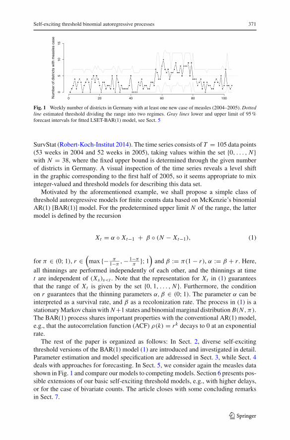
However, these SETINAR models are of little use for modeling time series takingvalues over a finite range of counts. As an illustrative example of a time series ofcounts exhibiting two different regimes over a bounded interval, Fig. 1 shows a timeseries plot of the counts of districts in Germany in which at least one new case ofmeasles was observed (weekly counts, 2004–2005); the data were downloaded from
123
Self-exciting threshold binomial autoregressive processes 371
0 20 40 60 80 100
05
1015
Num
ber
of d
istr
icts
with
mea
sles
cas
e
Fig. 1 Weekly number of districts in Germany with at least one new case of measles (2004–2005). Dottedline estimated threshold dividing the range into two regimes. Gray lines lower and upper limit of 95%forecast intervals for fitted LSET-BAR(1) model, see Sect. 5
SurvStat (Robert-Koch-Institut 2014). The time series consists of T = 105 data points(53 weeks in 2004 and 52 weeks in 2005), taking values within the set {0, . . . , N }with N = 38, where the fixed upper bound is determined through the given numberof districts in Germany. A visual inspection of the time series reveals a level shiftin the graphic corresponding to the first half of 2005, so it seems appropriate to mixinteger-valued and threshold models for describing this data set.
Motivated by the aforementioned example, we shall propose a simple class ofthreshold autoregressive models for finite counts data based on McKenzie’s binomialAR(1) [BAR(1)] model. For the predetermined upper limit N of the range, the lattermodel is defined by the recursion
Xt = α ◦ Xt−1 + β ◦ (N − Xt−1), (1)
for π ∈ (0; 1), r ∈(max {− π
1−π,− 1−π
π}; 1
)and β := π(1 − r), α := β + r . Here,
all thinnings are performed independently of each other, and the thinnings at timet are independent of (Xs)s<t . Note that the representation for Xt in (1) guaranteesthat the range of Xt is given by the set {0, 1, . . . , N }. Furthermore, the conditionon r guarantees that the thinning parameters α, β ∈ (0; 1). The parameter α can beinterpreted as a survival rate, and β as a recolonization rate. The process in (1) is astationaryMarkov chainwith N+1 states and binomialmarginal distribution B(N , π).The BAR(1) process shares important properties with the conventional AR(1) model,e.g., that the autocorrelation function (ACF) ρ(k) = rk decays to 0 at an exponentialrate.
The rest of the paper is organized as follows: In Sect. 2, diverse self-excitingthreshold versions of the BAR(1) model (1) are introduced and investigated in detail.Parameter estimation and model specification are addressed in Sect. 3, while Sect. 4deals with approaches for forecasting. In Sect. 5, we consider again the measles datashown in Fig. 1 and compare our models to competing models. Section 6 presents pos-sible extensions of our basic self-exciting threshold models, e.g., with higher delays,or for the case of bivariate counts. The article closes with some concluding remarksin Sect. 7.
123
372 T. A. Möller et al.
2 A basic self-exciting threshold binomial AR(1) model
Based on the BAR(1) model (1), we build our extension by introducing a self-excitingthreshold mechanism. For the moment, we restrict to a basic model, where the finiterange is separated into two regimes, and where the state of the process is selectedaccording to the previous observation (delay 1); later in Sect. 6, a number of pos-sible extensions of our basic model are presented. The two regimes are determinedby a specified threshold value 0 ≤ R < N : The lower regime consists of the states{0, 1, 2, . . . , R}, and the upper regime consists of {R + 1, R + 2, . . . , N }. In eachregime, the model takes individual values for the survival rate αi and for the recolo-nization rate βi .
2.1 The SET binomial AR(1) model
We start with the most general definition of our basic self-exciting threshold bino-mial AR(1) model (SET-BAR), i.e., a univariate model having two regimes and delayparameter 1. Later in Sect. 6, we discuss possible extensions to higher-order autore-gressions, to delays d > 1, to more than two regimes, and to the bivariate case.
Definition 2.1 Let N ∈ N be the predetermined upper limit of the range, and let 0 ≤R < N be the threshold value. Define πi ∈ (0; 1), ri ∈
(max {− πi
1−πi, − 1−πi
πi}; 1
),
as well as βi := πi · (1 − ri ) ∈ (0; 1) and αi := βi + ri ∈ (0; 1) for i ∈ {1, 2}. Aprocess (Xt ) is called a SET-BAR(1) process if Xt follows the recursion
Xt = φt ◦ Xt−1 + ηt ◦ (N − Xt−1) for t ∈ Z, (2)
where φt := α1 It−1 + α2(1 − It−1) and ηt := β1 It−1 + β2(1 − It−1) with It−1 :=1{Xt−1≤R} as the indicator variable.Note that, in the case R = 0, the parameter α1 has no influence on themodel and hencecan be chosen arbitrarily, which, in turn, makes α1 unidentifiable during the parameterestimation process. The same issue occurs for β2 in the case R = N−1. To circumventthese problems, we set r1 = r2 for the threshold values R = 0, N − 1, i.e., we use theLSET model as introduced in Sect. 2.2 below. In all remaining cases, the parametersare identifiable as long as there is a sufficient number of different observations in eachregime.
Since the SET-BAR(1) model falls within the class of density-dependent binomialAR(1) [DD-BAR(1)] models as introduced by Weiß and Pollett (2014),1 it followsby expression (1) in Weiß and Pollett (2014) that the transition probabilities pk|l :=P(Xt = k|Xt−1 = l) of the SET-BAR(1) process take the form
pk|l =min {k,l}∑
m=max {0,k+l−N }( lm
)(N−lk−m
)φmt (1 − φt )
l−mηk−mt (1 − ηt )
N−l+m−k > 0. (3)
1 The density-dependent models by Weiß and Pollett (2014) might also be understood as special SETmodels with N + 1 regimes.
123
Self-exciting threshold binomial autoregressive processes 373
Note that the (N +1)× (N +1)-dimensional transition matrix P := (pk|l)k,l=0,...,N isprimitive so that the process is ergodic with uniquely determined stationary marginaldistribution p. Since it is hardly possible to obtain a closed-form expression for the sta-tionary marginal distribution p, we determine it numerically by solving the eigenvalueproblem P p = p.
Next, we derive marginal conditional moments. From expression (2) in Weiß andPollett (2014), we obtain
E[Xt |Xt−1] = It−1 (r1Xt−1+(1 − r1)π1N )+(1 − It−1) (r2Xt−1 + (1 − r2)π2N ) ,
(4)
V [Xt |Xt−1] = It−1 (r1(1 − r1)(1 − 2π1)Xt−1 + N (1 − r1)π1 (1 − (1 − r1)π1))
+ (1 − It−1) (r2(1 − r2)(1 − 2π2)Xt−1
+ N (1 − r2)π2 (1 − (1 − r2)π2)) . (5)
Nowwe are prepared to obtain the unconditional mean and the variance of the station-ary process. For simplicity in notation, we define p := P(Xt ≤ R) = E[It−1],μX := E[Xt ], σ 2
X := V [Xt ], and the partial moments μI X := E[It−1Xt−1],μI X,2 := E[It−1X2
t−1]. Then, unconditional mean and variance are given by
μX = r1 − r21 − r2
μI X + N
(p π1
1 − r11 − r2
+ (1 − p) π2
), (6)
(1 − r22 ) σ 2X = r2(1 − r2)(1 − 2π2) μX − 2Npr2 ((1 − r1)π1 − (1 − r2)π2) μX
− 2r2(r1 − r2) μXμI X + (r21 − r22 ) μI X,2 − (r1 − r2)2 μ2
I X
+ 2N (r1 − p(r1 − r2)) ((1 − r1)π1 − (1 − r2)π2) μI X
+ (r1(1 − r1)(1 − 2π1) − r2(1 − r2)(1 − 2π2)) μI X
+ Np(1 − r1)π1 (1 − (1 − r1)π1)
+ N (1 − p)(1 − r2)π2 (1 − (1 − r2)π2)
+ N 2 p(1 − p) ((1 − r1)π1 − (1 − r2)π2)2 . (7)
The proof of (6) and (7) can be found in “Unconditional mean and variance” sectionof Appendix 1. Keep in mind that p strongly depends on π1 and π2.
2.2 The LSET binomial AR(1) model
Looking at Fig. 1, it becomes clear that the level of the measles time series is shiftedin the first half of 2005, while there is no obvious change in the serial dependencestructure. This motivates to consider the model in Definition 2.1 but with the addi-tional restriction r1 = r2 =: r with r ∈
(max {− π1
1−π1, − π2
1−π2, − 1−π1
π1, − 1−π2
π2}; 1
).
Notice that we will not have to consider the complicated restriction on the left-handside of the interval for r if we only use positive values for the dependence parameter r .
The restriction r1 = r2 is attractive to keep the number of model parameters low.It implies that α1 − β1 = α2 − β2 and that β2 − β1 = (π2 − π1)(1 − r). Since only
123
374 T. A. Möller et al.
the level of the process is shifted, we will refer to this model as the level SET-BAR(1)model, abbreviated as LSET-BAR(1) model.
Definition 2.2 A SET-BAR(1) process for which r1 = r2 =: r �= 0 holds is called anLSET-BAR(1) process.
Although in this case, the transition probabilities in (3) do not change much, we getmore simple expressions for the conditional moments (4) and (5):
E[Xt |Xt−1] = r Xt−1 + N (1 − r) (It−1 π1 + (1 − It−1) π2) , (8)
V [Xt |Xt−1] = It−1 (r(1 − r)(1 − 2π1)Xt−1 + N (1 − r)π1 (1 − (1 − r)π1))
+ (1 − It−1) (r(1 − r)(1 − 2π2)Xt−1
+ N (1 − r)π2 (1 − (1 − r)π2)) . (9)
In particular, unconditional mean (6) and variance (7) can be simplified a lot fora stationary LSET-BAR(1) process (Xt ); see “Unconditional mean and variance”section of Appendix 1:
μX = Np π1 + N (1 − p) π2, (10)
σ 2X = Np π1(1 − π1) + N (1 − p) π2(1 − π2) + N 2 p(1 − p) (π2 − π1)
2
+ 2r
1 + r(N − 1) (π2 − π1) (Np π1 − μI X ) . (11)
In view of the practical relevance of the parsimonious LSET model, additional sto-chastic properties are derived in Sect. 2.4 below.
2.3 The LSET0 binomial AR(1) model
Relations (8) and (9) highlight that the case r = 0 has to be treated separately. Incontrast to the usual BAR(1) model, where r = 0 corresponds to serial independence,an LSET-BAR(1) model with r = 0 still exhibits dependence on Xt−1, but onlythrough the indicator function It−1, whereas the concrete value of Xt−1 is withoutinfluence.
Definition 2.3 A SET-BAR(1) process with r1 = r2 = 0 is said to be an LSET0-BAR(1) process.
Notice that this model has only two parameters, namely π1 = α1 = β1 and π2 =α2 = β2. So depending on whether Xt−1 ≤ R or Xt−1 > R, the next count Xt isgenerated from either B(N , π1) or B(N , π2), respectively. If, for instance, R = 0, theLSET0 model allows for a simple way of causing zero inflation or zero deflation.
Conditional mean and variance follow from (8) and (9) as
E[Xt |Xt−1] = N (It−1 π1 + (1 − It−1) π2) , (12)
V [Xt |Xt−1] = It−1 (Nπ1(1 − π1)) + (1 − It−1) (Nπ2(1 − π2)) . (13)
123

Self-exciting threshold binomial autoregressive processes 375
The unconditional mean (10) remains as before, but the unconditional variance (11)simplifies to
σ 2X = Np π1(1 − π1) + N (1 − p) π2(1 − π2) + N 2 p(1 − p) (π2 − π1)
2.
(14)
We conclude our discussion by pointing out the analogy of the LSET0 model to the“piecewise constant AR model” in Example 4.3 in Tong (2011) as well as to the“martingale difference model” (Tong 2011, Example 4.4) [also see the more gen-eral threshold model for conditional heteroscedasticity (“T-CHARM”) in Chan et al.2014]. But while the latter models only change either the conditional mean or theconditional variance, the LSET0 model changes conditional mean and conditionalvariance simultaneously due to the conditional binomial distribution.
2.4 Further properties of the LSET-BAR(1) model
Let us look back to the LSET-BAR(1)model according to Definition 2.2. The binomialindex of dispersion, BID, is a useful metric when quantifying the dispersion behaviorof count data random variables with a finite range {0, . . . , N }. It is defined as
BID ≡ BID(N , μ, σ 2) = Nσ 2
μ(N − μ)= σ 2
μ(1 − μ
N
) > 0. (15)
For the binomial distribution, it holds that BID = 1. A distribution with finite range issaid to have overdispersion if BID > 1 (also extra-binomial variation), it is equidis-persed if BID = 1, and it is underdispersed if BID < 1, each with respect to thebinomial distribution.
For the LSET-BAR(1) model, the BID follows from (10) and (11) as
BID = 1 + N (N−1)p(1 − p) (π2 − π1)2+ 2r
1+r (N − 1)(π2 − π1) (Np π1 − μI X )
Np π1(1 − π1)+N (1 − p) π2(1 − π2)+Np(1 − p) (π2 − π1)2,
(16)
see “Binomial index of dispersion” section of Appendix 1. Note that for r ∈(0; 1), underdispersion is only possible for π2 < π1. In contrast, for r ∈(max {− π1
1−π1, − π2
1−π2, − 1−π1
π1, − 1−π2
π2}; 0
), underdispersion is only possible for
π2 > π1. For r = 0 (LSET0 model, see Definition 2.3), the model always showsoverdispersion provided that π1 �= π2.
Solving now the equation BID = 1 in order to x := π2 − π1, it follows that
0 = N (N − 1)p(1 − p) · x2 + 2r
1 + r(N − 1) (Npπ1 − μI X ) · x
⇔ x = 0 (⇔ π1 = π2) or x = −2r1+r (Npπ1 − μI X )
Np(1 − p).
123
376 T. A. Möller et al.
040302010
0.00
0.04
0.08
State
Den
sity
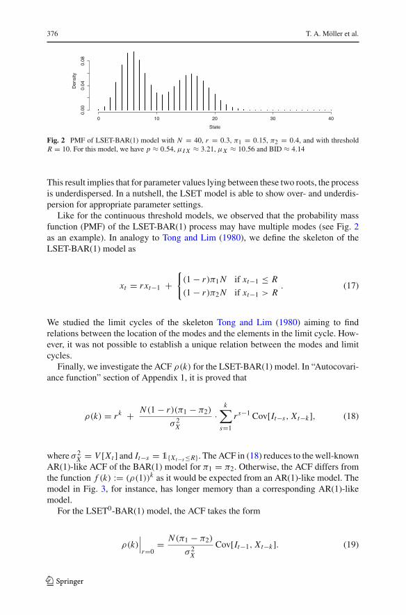
Fig. 2 PMF of LSET-BAR(1) model with N = 40, r = 0.3, π1 = 0.15, π2 = 0.4, and with thresholdR = 10. For this model, we have p ≈ 0.54, μI X ≈ 3.21, μX ≈ 10.56 and BID ≈ 4.14
This result implies that for parameter values lying between these two roots, the processis underdispersed. In a nutshell, the LSET model is able to show over- and underdis-persion for appropriate parameter settings.
Like for the continuous threshold models, we observed that the probability massfunction (PMF) of the LSET-BAR(1) process may have multiple modes (see Fig. 2as an example). In analogy to Tong and Lim (1980), we define the skeleton of theLSET-BAR(1) model as
xt = r xt−1 +{
(1 − r)π1N if xt−1 ≤ R
(1 − r)π2N if xt−1 > R. (17)
We studied the limit cycles of the skeleton Tong and Lim (1980) aiming to findrelations between the location of the modes and the elements in the limit cycle. How-ever, it was not possible to establish a unique relation between the modes and limitcycles.
Finally, we investigate the ACF ρ(k) for the LSET-BAR(1) model. In “Autocovari-ance function” section of Appendix 1, it is proved that
ρ(k) = rk + N (1 − r)(π1 − π2)
σ 2X
·k∑
s=1
rs−1 Cov[It−s, Xt−k], (18)
where σ 2X = V [Xt ] and It−s = 1{Xt−s≤R}. The ACF in (18) reduces to the well-known
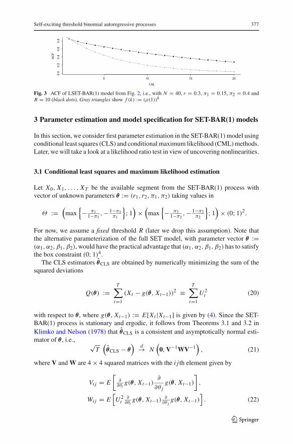
AR(1)-like ACF of the BAR(1) model for π1 = π2. Otherwise, the ACF differs fromthe function f (k) := (ρ(1))k as it would be expected from an AR(1)-like model. Themodel in Fig. 3, for instance, has longer memory than a corresponding AR(1)-likemodel.
For the LSET0-BAR(1) model, the ACF takes the form
ρ(k)∣∣∣r=0
= N (π1 − π2)
σ 2X
Cov[It−1, Xt−k]. (19)
123
Self-exciting threshold binomial autoregressive processes 377
Fig. 3 ACF of LSET-BAR(1) model from Fig. 2, i.e., with N = 40, r = 0.3, π1 = 0.15, π2 = 0.4 andR = 10 (black dots). Gray triangles show f (k) := (ρ(1))k
3 Parameter estimation and model specification for SET-BAR(1) models
In this section, we consider first parameter estimation in the SET-BAR(1) model usingconditional least squares (CLS) and conditionalmaximum likelihood (CML)methods.Later, we will take a look at a likelihood ratio test in view of uncovering nonlinearities.
3.1 Conditional least squares and maximum likelihood estimation
Let X0, X1, . . . , XT be the available segment from the SET-BAR(1) process withvector of unknown parameters θ := (r1, r2, π1, π2) taking values in
Θ :=(max
{− π1
1−π1,− 1−π1
π1
}; 1
)×
(max
{− π2
1−π2,− 1−π2
π2
}; 1
)× (0; 1)2.
For now, we assume a fixed threshold R (later we drop this assumption). Note thatthe alternative parameterization of the full SET model, with parameter vector θ :=(α1, α2, β1, β2), would have the practical advantage that (α1, α2, β1, β2) has to satisfythe box constraint (0; 1)4.
The CLS estimators θ̂CLS are obtained by numerically minimizing the sum of thesquared deviations
Q(θ) :=T∑t=1
(Xt − g(θ, Xt−1))2 ≡
T∑t=1
U 2t (20)
with respect to θ , where g(θ, Xt−1) := E[Xt |Xt−1] is given by (4). Since the SET-BAR(1) process is stationary and ergodic, it follows from Theorems 3.1 and 3.2 inKlimko and Nelson (1978) that θ̂CLS is a consistent and asymptotically normal esti-mator of θ , i.e., √
T(θ̂CLS − θ
)d→ N
(0, V−1WV−1
), (21)
where V and W are 4 × 4 squared matrices with the i j th element given by
Vi j = E
[∂
∂θig(θ, Xt−1)
∂
∂θ jg(θ, Xt−1)
],
Wi j = E[U 2t
∂∂θi
g(θ, Xt−1)∂
∂θ jg(θ, Xt−1)
]. (22)
123

378 T. A. Möller et al.
Similar arguments apply to theLSETmodelswith their reduced number of parameters.Consider now the conditional maximum likelihood (CML) method to estimate the
unknown model parameters θ . The CML estimators are obtained maximizing theconditional log-likelihood function
�(θ) := log L(θ; x0) ≡T∑t=1
ln Pθ (Xt = xt |Xt−1 = xt−1), (23)
with the transition probabilities defined in (3), i.e., they solve the following maximiza-tion problem:
θ̂ = argmaxθ∈Θ �(θ). (24)
Note that no closed-form expressions for the estimates can be found, so numericalprocedures have to be employed. In order to prove the existence and consistency of theCML estimators, it is sufficient to show that Condition 5.1 of Billingsley (1961) holds.If Condition 5.1 holds, then Theorems 2.1 and 2.2 of Billingsley (1961) guarantee thatthere exists a consistent CML estimator being asymptotically normally distributed,
√T
(θ̂ML − θ
)d→ N
(0, I−1
1 (θ))
, (25)
where I1(θ) denotes the expected Fisher information. Condition 5.1 of Billingsley(1961) is fulfilled provided that
1. the set D of (k, l) such that pk|l(θ) > 0 is independent of θ ;2. each pk|l(θ) has continuous partial derivatives of third-order throughout Θ;3. the d × w matrix
(∂pk|l(θ)
∂θu
)(k,l)∈D,u=1,...,w
has rank w throughout Θ , where d := |D| and w := dim(Θ);4. for each θ ∈ Θ , there is only one ergodic set and there are no transient states.
Conditions 1 and 4 are fulfilled since all pk|l > 0 as stated earlier, while Condition 2holds due to the polynomial structure of the pk|l . The third condition is also fulfilledif we exclude trivial cases such as π1 = π2 [BAR(1) model] or r = 0 (LSET0-BAR(1) model). Note that CML estimation for the usual BAR(1) model was alreadyinvestigated by Weiß and Kim (2013). For the LSET0 model, the parameter vectorreduces to θ = (π1, π2) ∈ (0; 1)2, and we have w = 2 in this case.
For the numerical maximization of the log-likelihood (23), we use the R functionoptim with the expected Fisher information I in (25) being approximated by thenegative Hessian of the log-likelihood at the maximum (observed Fisher information).The initial estimates required by such numerical procedures are obtained by the CLSapproach.
Next, we turn to the estimation of the threshold parameter. Note that R is a discrete-valued parameter in our case. Hence, it cannot be directly included in the parameter set
123
Self-exciting threshold binomial autoregressive processes 379
(a) (b)
(c) (d)
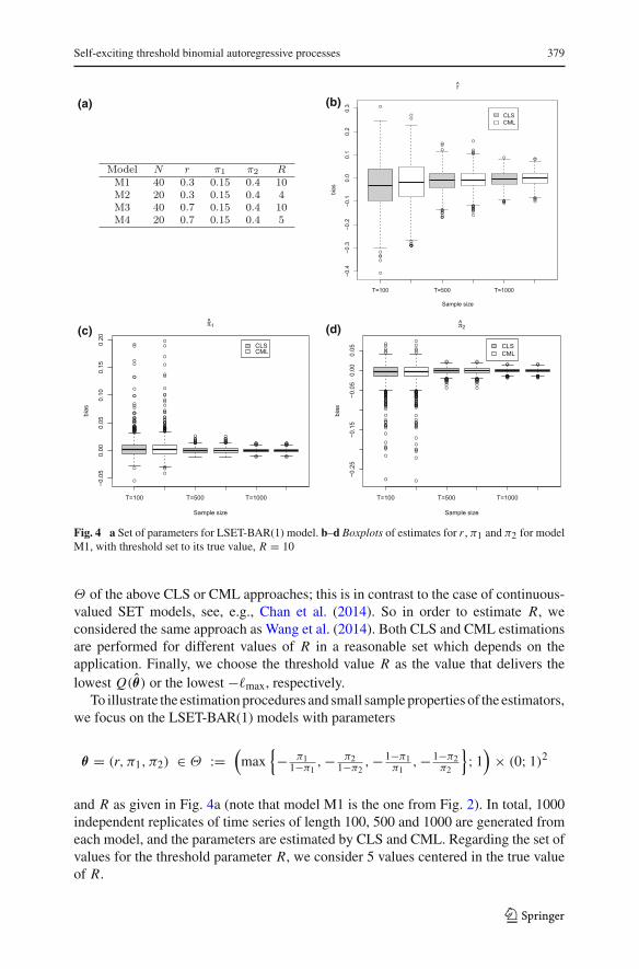
Fig. 4 a Set of parameters for LSET-BAR(1) model. b–d Boxplots of estimates for r , π1 and π2 for modelM1, with threshold set to its true value, R = 10
Θ of the above CLS or CML approaches; this is in contrast to the case of continuous-valued SET models, see, e.g., Chan et al. (2014). So in order to estimate R, weconsidered the same approach as Wang et al. (2014). Both CLS and CML estimationsare performed for different values of R in a reasonable set which depends on theapplication. Finally, we choose the threshold value R as the value that delivers thelowest Q(θ̂) or the lowest −�max, respectively.
To illustrate the estimationprocedures and small sample properties of the estimators,we focus on the LSET-BAR(1) models with parameters
θ = (r, π1, π2) ∈ Θ :=(max
{− π1
1−π1,− π2
1−π2,− 1−π1
π1,− 1−π2
π2
}; 1
)× (0; 1)2
and R as given in Fig. 4a (note that model M1 is the one from Fig. 2). In total, 1000independent replicates of time series of length 100, 500 and 1000 are generated fromeach model, and the parameters are estimated by CLS and CML. Regarding the set ofvalues for the threshold parameter R, we consider 5 values centered in the true valueof R.
123

380 T. A. Möller et al.
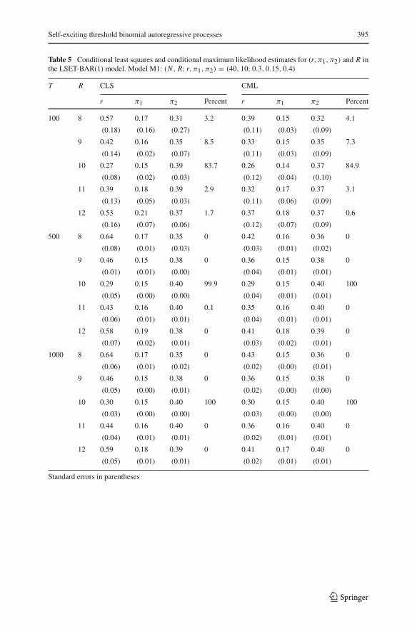
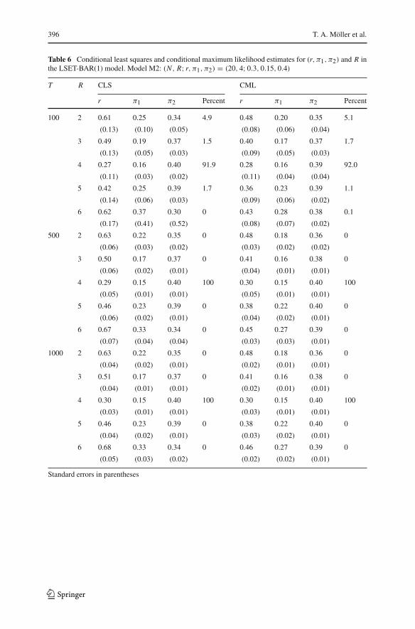
The results are summarized in Tables 5, 6, 7 and 8 in Appendix 2, while Fig. 4b–ddisplays boxplots of the biases for θ̂ . The tables report for each model the (mean)estimates and corresponding standard errors and, for each value of R, the percentageof series for which R leads to the minimum Q(θ̂) in the CLS or the lowest −�maxin the CML estimation. First, note that the strategy to estimate R allows choosingthe correct value most of the times already for small sample sizes, and this hit ratequickly approaches 100% for increasing T . This is similar to the case of the SETPARmodels studied by Wang et al. (2014), where a formal proof of the consistency of theestimation approach for R is given. Tables 5, 6, 7 and 8 also illustrate the unbiasednessand consistency of the estimators θ̂ , since the bias and standard errors decrease tozero as T increases. Furthermore, Fig. 4 illustrates the small sample properties ofthe estimators: The componentwise estimates tend to be unbiased and consistent. Theresults furthermore indicate that the CLS estimates present larger biases than CMLwhen obtained under an incorrect value of the threshold.
3.2 Likelihood ratio test
Let us now tackle the issue of testing for nonlinearity in the data. Petruccelli (1990)investigated the performance of different tests for SETAR-type nonlinearity and con-cluded that the likelihood ratio (LR) test was one of the best performers. Hence, weconsider an LR test in the sequel, with the null hypothesis of a BAR(1) model. Inorder to prove the applicability of the test, we consider again the results in Billingsley(1961). Let Φ be the parameter set of the BAR(1) model and Θ be the one of theSET-BAR(1) model with specified threshold value R. We can define h : Φ → Θ as amapping from Φ into Θ in such a way that r1 = r2 = r and π1 = π2 = π . This map-ping satisfies Condition 3.1 of Billingsley (1961). Together with Condition 5.1, whichis fulfilled as already shown before, Theorem 5.2 of Billingsley (1961) is applicable:If θ0 = h(φ0) is the true parameter value, then
2
(max
Θ� − max
Φ�
)d→ χ2
w−c, (26)
where w := dim(Θ) and c := dim(Φ). For the set model, w = 4 and c = 2, so theLR statistic converges to a χ2
2 distribution. If we choose the LSET model instead, wehave a convergence to a χ2
1 distribution. The finite-sample performance of the LR testis briefly considered in Sect. 5 below.
4 Forecasting for SET-BAR(1) models
To forecast a SET-BAR(1) process, we use the forecasting distributions over all hori-zons h ∈ N, i.e., the probabilistic distribution of XT+h based on the observed timeseries up to time T (“more-than-one-step-ahead predictive distributions,” see Tong2011). This approach leads to forecasts being themselves counts and therefore beingcoherent with the sample space. It also allows the quantification of the uncertainty
123

Self-exciting threshold binomial autoregressive processes 381
0 10 20 30 40
0.00
0.10
0.20
XT+1
prob
0 10 20 30 40
0.00
0.10
0.20
XT+10
prob
0 10 20 30 40
0.00
0.10
0.20
XT+25
prob
0 10 20 30 40
0.00
0.10
0.20
XT+50
prob
Fig. 5 Forecasting distributions for model M1 conditional on XT = 2
0 10 20 30 40
0.00
0.10
0.20
XT+1
prob
0 10 20 30 40
0.00
0.10
0.20
XT+10
prob
0 10 20 30 40
0.00
0.10
0.20
XT+25
prob
0 10 20 30 40
0.00
0.10
0.20
XT+50
prob
Fig. 6 Forecasting distributions for model M1 conditional on XT = 12
associated with the future counts, which is important in a context of risk analysis.Point forecasts, if needed, are easily obtained from the median or the mode of theforecasting distribution. For the SET-BAR(1) process, the h-step-ahead conditionaldistribution of XT+h given XT is given by
P(XT+h = xT+h | XT = xT ) = [Ph]xT+h ,xT , (27)
where P denotes the transition matrix defined via (3). To prove (27), note that the con-ditional distribution of XT+h given XT satisfies the Chapman–Kolmogorov equations,since we are concerned with a homogeneous Markov chain.
As an illustration, Figs. 5 and 6 represent the forecasting distributions for thehorizons h = 1, 10, 25, 50 steps ahead for model M1, i.e., (N , R; r, π1, π2) =(40, 10; 0.3, 0.15, 0.4), conditioned on an observation in each of the two regimes,XT = 2 and XT = 12, respectively. The figures show how, for growing h, these
123
382 T. A. Möller et al.
Table 1 Estimated bias and MSEs for median forecasts in models M1–M4
T … over all conditional distributions … conditional on
100 500 1000 XT = 2 XT = 12
100 500 1000 100 500 1000
M1 Bias −0.2448 −0.0645 −0.0235 −0.1198 −0.1680 −0.0960 −0.3925 −0.1690 −0.0940
MSE 2.1327 0.4273 0.2493 0.5348 0.1700 0.0960 1.1754 0.1750 0.0940
M2 Bias −0.0348 −0.0001 0.0117 −0.2457 −0.2690 −0.1760 0.0819 0.0580 0.0140
MSE 0.6619 0.1942 0.1239 0.4681 0.2690 0.1760 0.3428 0.0620 0.0140
M3 Bias −0.2711 −0.0556 −0.0327 −0.2592 −0.0060 0 −0.1704 −0.0120 −0.0040
MSE 1.3139 0.1998 0.1346 0.4840 0.0060 0 1.0533 0.0260 0.0040
M4 Bias −0.1667 −0.0401 −0.0297 −0.0866 0 0 −0.3454 −0.0380 −0.0040
MSE 0.4939 0.1423 0.0994 0.0866 0 0 0.4814 0.0380 0.0040
distributions converge to the stationary marginal distribution from Fig. 2, as expectedfrom the ergodicity of the process.
To assess the accuracy of the probabilistic forecasting in the case of estimatedparameters, we use an approach suggested by Corradi and Swanson (2006), whichmeasures accuracy using a distributional analog of mean squared error. Focussingon the one-step-ahead forecast distribution, i.e., h = 1, we denote the conditionaldistribution P(XT+1 = i | XT = j) by fi | j with i, j ∈ 0, 1, . . . , N . Then, themean squared error of the estimator f̂·| j for the predictive distribution f·| j is theaverage over the support i ∈ {0, 1, . . . , N } of E[( f̂i | j − fi | j )2] (note that the bias1
N+1
∑Ni=0 E( f̂i | j − fi | j ) across the full support is equal to 0 since both the estimated
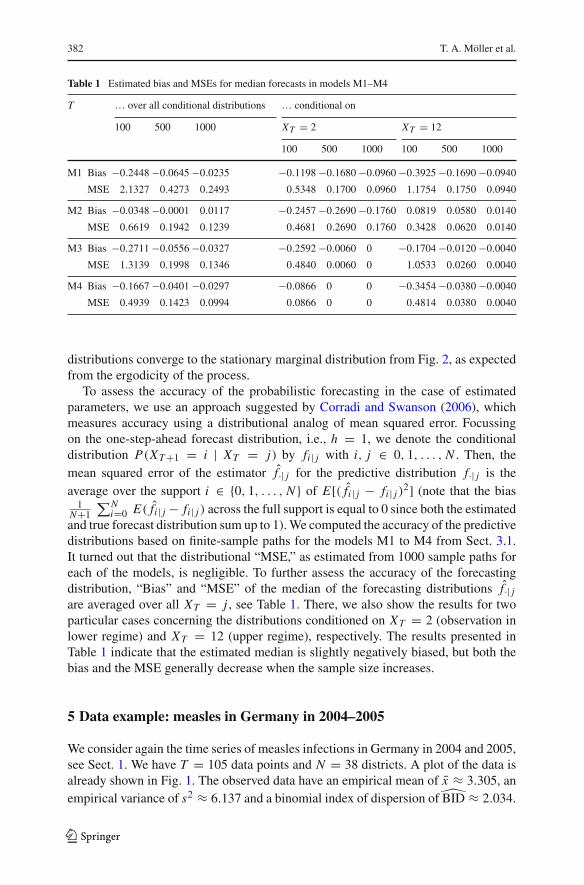
and true forecast distribution sum up to 1).We computed the accuracy of the predictivedistributions based on finite-sample paths for the models M1 to M4 from Sect. 3.1.It turned out that the distributional “MSE,” as estimated from 1000 sample paths foreach of the models, is negligible. To further assess the accuracy of the forecastingdistribution, “Bias” and “MSE” of the median of the forecasting distributions f̂·| jare averaged over all XT = j , see Table 1. There, we also show the results for twoparticular cases concerning the distributions conditioned on XT = 2 (observation inlower regime) and XT = 12 (upper regime), respectively. The results presented inTable 1 indicate that the estimated median is slightly negatively biased, but both thebias and the MSE generally decrease when the sample size increases.
5 Data example: measles in Germany in 2004–2005
We consider again the time series of measles infections in Germany in 2004 and 2005,see Sect. 1. We have T = 105 data points and N = 38 districts. A plot of the data isalready shown in Fig. 1. The observed data have an empirical mean of x̄ ≈ 3.305, anempirical variance of s2 ≈ 6.137 and a binomial index of dispersion of B̂ID ≈ 2.034.
123

Self-exciting threshold binomial autoregressive processes 383
Fig. 7 Plot of SACF for measles data (2004–2005)
Table 2 Comparison of theLSET’s CML estimates fordifferent threshold values
Standard errors are given inparentheses
R r π1 π2 −�max
3 0.2546 0.0681 0.1174 217.62
(0.0907) (0.0074) (0.0114)
4 0.2245 0.0697 0.1376 215.05
(0.0906) (0.0063) (0.0142)
5 0.1947 0.0707 0.1604 212.28
(0.0876) (0.0057) (0.0169)
6 0.3083 0.0787 0.1482 218.24
(0.0744) (0.0065) (0.0229)
7 0.3381 0.0813 0.1594 218.81
(0.0679) (0.0066) (0.0299)
We have tested for overdispersion by using the approach of Weiß and Kim (2014)and found that the data are significantly overdispersed on a 5% level. The plot of thesample ACF (SACF) in Fig. 7 shows a slowly decaying extend of serial dependence.
In view of the level shift being visible in Fig. 1, we start with fitting an LSETmodel to the data (later, we also consider the more general SET model and the morespecial LSET0 model). We estimate the model parameters for threshold values ofR ∈ {3, . . . , 7}, which is a reasonable range when we take a look at the plot of the datain Fig. 1. The estimates given different threshold values R are compared in Table 2.Looking at−�max, we decide to consider amodel with a threshold value of R = 5, alsosee Fig. 1. The initial values for the CML estimation procedure were obtained fromthe CLS estimates computed for threshold values of R ∈ {3, . . . , 7}. The thresholdvalue that minimizes Q(θ) from Eq. (20) is also R = 5, and the corresponding CLSestimates are r̂ = 0.28, π̂1 = 0.06 and π̂2 = 0.15.
We also applied the LR test of Sect. 3.2 to check whether such a nonlinear model isappropriate for the data. For the LSET-BAR(1) model against the BAR(1) model byMcKenzie (1985) (also see Table 4 below), we obtain a value about 19.6 for the LR teststatistic, while our critical value on a 5% level is given by χ2
1;0.95 = 3.841. So we haveto reject the null hypothesis of a BAR(1) model. In order to verify the applicability ofthe LR test from Sect. 3.2 for this data example, we simulated n = 1000 paths of theBAR(1) model with the estimated parameters from Table 4 for different time serieslength T = 100, 500, 1000 (with T = 100 being close to our data). We calculated thetest statistic for the SET- and LSET-BAR(1) model and studied, among others, the size
123
384 T. A. Möller et al.
Table 3 Simulated sizesconcerning the critical valuesχ22,0.95 (SET-BAR(1) model)
and χ21,0.95 (LSET-BAR(1)
model), respectively
T = 100 T = 500 T = 1000
SET-BAR(1) 0.053 0.049 0.049
LSET-BAR(1) 0.045 0.043 0.048
Table 4 Comparison of estimated parameters (standard errors in parentheses) for different models formeasles data
Par. 1 Par. 2 Par. 3 Par. 4 AIC BIC
BAR(1) 0.0882 0.4158 – – 448.2 453.5
(π, r) (0.0070) (0.0550)
DD-BAR(1) 0.0419 0.5270 0 – 436.9 444.9
(a, b, r) (0.0095) (0.1077) (0.1765)
Bin. INARCH(1) 0.0419 0.5270 – – 434.9 440.2
(a, b) (0.0060) (0.0682)
SET-BAR(1) 0.0706 0.1558 0.1916 0.2904 432.5 443.1
(π1, π2, r1, r2) (0.0056) (0.0269) (0.0884) (0.375)
LSET-BAR(1) 0.0707 0.1604 0.1947 – 430.6 438.5
(π1, π2, r) (0.0057) (0.0169) (0.0876)
LSET0-BAR(1) 0.0689 0.1671 – – 433.4 438.7
(π1, π2) (0.0045) (0.0135)
All threshold models include a threshold value of R = 5
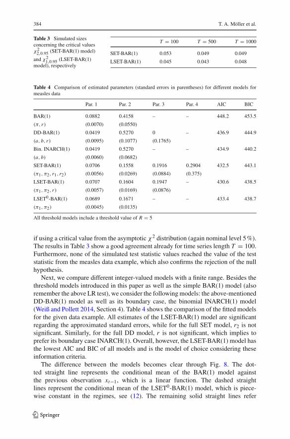
if using a critical value from the asymptotic χ2 distribution (again nominal level 5%).The results in Table 3 show a good agreement already for time series length T = 100.Furthermore, none of the simulated test statistic values reached the value of the teststatistic from the measles data example, which also confirms the rejection of the nullhypothesis.
Next, we compare different integer-valued models with a finite range. Besides thethreshold models introduced in this paper as well as the simple BAR(1) model (alsoremember the above LR test), we consider the followingmodels: the above-mentionedDD-BAR(1) model as well as its boundary case, the binomial INARCH(1) model(Weiß and Pollett 2014, Section 4). Table 4 shows the comparison of the fitted modelsfor the given data example. All estimates of the LSET-BAR(1) model are significantregarding the approximated standard errors, while for the full SET model, r2 is notsignificant. Similarly, for the full DD model, r is not significant, which implies toprefer its boundary case INARCH(1). Overall, however, the LSET-BAR(1) model hasthe lowest AIC and BIC of all models and is the model of choice considering theseinformation criteria.
The difference between the models becomes clear through Fig. 8. The dot-ted straight line represents the conditional mean of the BAR(1) model againstthe previous observation xt−1, which is a linear function. The dashed straightlines represent the conditional mean of the LSET0-BAR(1) model, which is piece-wise constant in the regimes, see (12). The remaining solid straight lines refer
123
Self-exciting threshold binomial autoregressive processes 385
1086420
02
46
810
Fig. 8 Dots represent observed frequencies for measles data with coordinates (xt−1, xt ). Lines representconditional means for BAR(1) (dotted), LSET-BAR(1) (solid) and LSET0-BAR(1) (dashed)
0 10 20 30
0.00
0.15
0.30
XT+1
prob
0 10 20 300.
000.
150.
30
XT+2
prob
0 10 20 30
0.00
0.15
0.30
XT+3
prob
0 10 20 30
0.00
0.15
0.30
XT+4
prob
Fig. 9 Forecast distribution for 1, 2, 3 and 4 weeks ahead, conditioned on x105 = 2, for the number ofdistricts with new measles infections
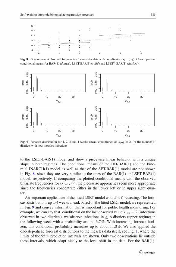
to the LSET-BAR(1) model and show a piecewise linear behavior with a uniqueslope in both regimes. The conditional means of the DD-BAR(1) and the bino-mial INARCH(1) model as well as that of the SET-BAR(1) model are not shownin Fig. 8, since they are very similar to the ones of the BAR(1) or LSET-BAR(1)model, respectively. If comparing the plotted conditional means with the observedbivariate frequencies for (xt−1, xt ), the piecewise approaches seem more appropriatesince the frequencies concentrate either in the lower left or in upper right quar-ter.
An important application of the fitted LSET model would be forecasting. The fore-cast distributions up to 4weeks ahead, based on the fitted LSETmodel, are representedin Fig. 9 and convey information that is important for public health monitoring. Forexample, we can say that, conditional on the last observed value x105 = 2 (infectionsobserved in two districts), we observe infections in ≥ 6 districts (upper regime) inthe following week with a probability around 3.7%. With increasing forecast hori-zon, this conditional probability increases up to about 11.0%. We also applied theone-step-ahead forecast distributions to the measles data itself, see Fig. 1, where thelimits of the 95% prediction intervals are shown. Only two observations lie outsidethese intervals, which adapt nicely to the level shift in the data. For the BAR(1)-
123
386 T. A. Möller et al.
Number of districts
Den
sity
0.0
0.1
0.2
0.3
0.4
0 1 2 3 4 5 6 7 8 9 10
Fig. 10 Comparison of histogram of measles data (bars) and marginal distribution of fitted LSET model(ticks). 95% confidence bands from parametric bootstrap (black lines)
based forecasts instead (not shown), the 95% bands look clearly worse, which againconfirms preferring the LSET model for our measles data. Generally, if looking atthe coverage rates of the one-step-ahead prediction intervals for different levels, theBAR(1) model always performs worst, and the LSET0 model is second worst, whileall remaining models do comparably well in terms of this retrospective forecast-ing.
At this point, it is also interesting to look at a completely different approachtoward modeling the piecewise behavior. As already pointed out in Sect. 1, aparameter-driven alternative would be a (two-state) binomial HMM (Zucchini andMacDonald 2009). Although the estimates for the HMM’s transition matrix are notsignificant, there are well-interpretable analogies between the fitted HMM and theLSET-BAR(1) model. The estimated binomial parameters of the HMM are 0.0590in the lower and 0.1740 in the upper regime, which are fairly close to the esti-mates for π1, π2 in the LSET-BAR(1) model, the latter being 0.0707, 0.1604. Thestationary distribution in the HMM gives us a probability of 0.8132 to be in thelower regime, while the LSET-BAR(1) model results in p = 0.8905. So both typesof regime switching model lead to similar conclusions with respect to the measlesdata.
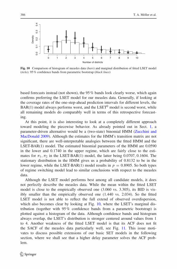
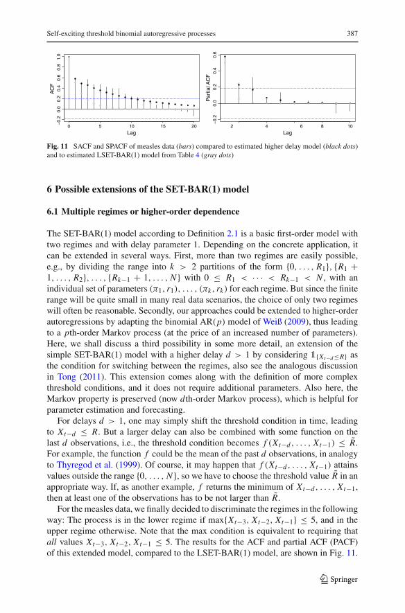
Although the LSET model performs best among all candidate models, it doesnot perfectly describe the measles data. While the mean within the fitted LSETmodel is close to the empirically observed one (3.060 vs. 3.305), its BID is vis-ibly smaller than the empirically observed one (1.440 vs. 2.034). So the fittedLSET model is not able to reflect the full extend of observed overdispersion,which also becomes clear by looking at Fig. 10, where the LSET’s marginal dis-tribution (together with 95% confidence bands from a parametric bootstrap) isplotted against a histogram of the data. Although confidence bands and histogramalways overlap, the LSET’s distribution is stronger centered around values from 1to 4. Another weakness of the fitted LSET model is that its ACF does not fitthe SACF of the measles data particularly well, see Fig. 11. This issue moti-vates to discuss possible extensions of our basic SET models in the followingsection, where we shall see that a higher delay parameter solves the ACF prob-lem.
123
Self-exciting threshold binomial autoregressive processes 387
0 5 10 15 20
−0.
20.
00.
20.
40.
60.
81.
0
Lag
AC
F
2 4 6 8 10
−0.
20.
00.
20.
40.
6
Lag
Par
tial A
CF
Fig. 11 SACF and SPACF of measles data (bars) compared to estimated higher delay model (black dots)and to estimated LSET-BAR(1) model from Table 4 (gray dots)
6 Possible extensions of the SET-BAR(1) model
6.1 Multiple regimes or higher-order dependence
The SET-BAR(1) model according to Definition 2.1 is a basic first-order model withtwo regimes and with delay parameter 1. Depending on the concrete application, itcan be extended in several ways. First, more than two regimes are easily possible,e.g., by dividing the range into k > 2 partitions of the form {0, . . . , R1}, {R1 +1, . . . , R2}, . . . , {Rk−1 + 1, . . . , N } with 0 ≤ R1 < · · · < Rk−1 < N , with anindividual set of parameters (π1, r1), . . . , (πk, rk) for each regime. But since the finiterange will be quite small in many real data scenarios, the choice of only two regimeswill often be reasonable. Secondly, our approaches could be extended to higher-orderautoregressions by adapting the binomial AR(p) model of Weiß (2009), thus leadingto a pth-order Markov process (at the price of an increased number of parameters).Here, we shall discuss a third possibility in some more detail, an extension of thesimple SET-BAR(1) model with a higher delay d > 1 by considering 1{Xt−d≤R} asthe condition for switching between the regimes, also see the analogous discussionin Tong (2011). This extension comes along with the definition of more complexthreshold conditions, and it does not require additional parameters. Also here, theMarkov property is preserved (now dth-order Markov process), which is helpful forparameter estimation and forecasting.
For delays d > 1, one may simply shift the threshold condition in time, leadingto Xt−d ≤ R. But a larger delay can also be combined with some function on thelast d observations, i.e., the threshold condition becomes f (Xt−d , . . . , Xt−1) ≤ R̃.For example, the function f could be the mean of the past d observations, in analogyto Thyregod et al. (1999). Of course, it may happen that f (Xt−d , . . . , Xt−1) attainsvalues outside the range {0, . . . , N }, so we have to choose the threshold value R̃ in anappropriate way. If, as another example, f returns the minimum of Xt−d , . . . , Xt−1,then at least one of the observations has to be not larger than R̃.
For themeasles data, we finally decided to discriminate the regimes in the followingway: The process is in the lower regime if max{Xt−3, Xt−2, Xt−1} ≤ 5, and in theupper regime otherwise. Note that the max condition is equivalent to requiring thatall values Xt−3, Xt−2, Xt−1 ≤ 5. The results for the ACF and partial ACF (PACF)of this extended model, compared to the LSET-BAR(1) model, are shown in Fig. 11.
123

388 T. A. Möller et al.
Obviously, we achieve a much better fit to both SACF and SPACF by this thresholdcondition, and the new model shows a much longer memory. Furthermore, mean(3.49), variance (5.83) and BID (1.84) of this model better agree with the empiricallyobserved values for the measles data.
6.2 A bivariate extension
The SET-BAR(1) process can also be generalized to the case of multivariate observa-tions. A possible extension is to induce piecewise-type patterns to the class of bivariatebinomial autoregressive models introduced by Scotto et al. (2014), which are basedon the bivariate binomial thinning operator “⊗,” defined via
(α1, α2, ϕα) ⊗ X | X ∼ BVBII (X1, X2,min{X1, X2};α1, α2, ϕα) . (28)
The definition of the SET-BVBII-AR(1) is given below.
Definition 6.1 Let N := [N1 N2]′ ∈ N2 be the vector of upper limits for the bivariate
range, let 0 ≤ R j < N j for j ∈ {1, 2} be the threshold values.
For i ∈ {0, 1}2 and j ∈ {1, 2}, let π(i)j ∈ (0; 1), and
r (i)j ∈
(max
{− π
(i)j
1 − π(i), −1 − π
(i)j
π(i)j
}; 1
).
In addition, define β(i)j := π
(i)j · (1 − r (i)
j ) ∈ (0; 1) and α(i)j := β
(i)j + r (i)
j ∈ (0; 1).Let α(i) := (α
(i)1 , α
(i)2 , ϕ
(i)α ) and β(i) := (β
(i)1 , β
(i)2 , ϕ
(i)β ).
The process (Xt ) of bivariate random variables Xt := [Xt,1 Xt,2]′ is calledSET-BVBII-AR(1) if Xt satisfies the recursion
Xt = φt ⊗ Xt−1 + ηt ⊗ (N − Xt−1) for t ∈ Z, (29)
where φt := α(I t−1), ηt := β(I t−1), and I t−1 := [1{Xt−1,1>R1} 1{Xt−1,2>R2}]′.Furthermore, it is assumed that the thinnings are performed independently of each
other.
So the bivariate indicator I t−1 distinguishes between the following events:
I t−1 = [0 0]′ iff {Xt−1,1 ≤ R1, Xt−1,2 ≤ R2};I t−1 = [0 1]′ iff {Xt−1,1 ≤ R1, Xt−1,2 > R2};I t−1 = [1 0]′ iff {Xt−1,1 > R1, Xt−1,2 ≤ R2};I t−1 = [1 1]′ iff {Xt−1,1 > R1, Xt−1,2 > R2}.
The transition probabilities at lag 1 of the SET-BVBII-AR(1) model are computedthrough the expression
123

Self-exciting threshold binomial autoregressive processes 389
pk|l := P(Xt = k | Xt−1 = l) ≡ P(φt ⊗ Xt−1 + ηt ⊗ (N − Xt−1) = k | Xt−1 = l
)
=min{k1,l1}∑
a1=0
min{k2,l2}∑a2=0
p(l1,l2;α(i))(a1, a2) p(N1−l1,N2−l2;β(i))(k1 − a1, k2 − a2),
where k := [k1 k2]′, l := [l1 12]′ as well as i := [1{l1>R1} 1{l2>R2}]′, and wherethe bivariate probability mass functions p(·)(·) defined as in equation (13) in Scottoet al. (2014, p. 236). Note that since these transition probabilities are truly positive,the SET-BVBII-AR(1) process is a primitive and finite-state Markov chain, which, inturn, implies irreducibility and aperiodicity. Hence, a uniquely determined stationarymarginal distribution exists. Denoting the transition matrix by P := (pk|l ), the uniquestationary marginal distribution, expressed as a vector p, is obtained as the solutionof the linear equation P p = p.
Now we are prepared to obtain the mean, the variance and the autocovariancefunction of the process. For simplicity in notation, we define qi := P(I t−1 = i)and u j,i := E[Xt−1, j |I t−1 = i], σ 2
j,i := V [Xt−1, j |I t−1 = i] for i ∈ {0, 1}2 andj ∈ {1, 2}. The mean of the process is given by
E[Xt ] =∑i
qi
[α
(i)1 u1,i + β
(i)1 ν1,i
α(i)2 u2,i + β
(i)2 ν2,i
].
In order to calculate the variance (componentwise), note first that
V [Xt ] = V[φt ⊗ Xt−1 + ηt ⊗ (N − Xt−1)
]= V
[φt ⊗ Xt−1
] + V[ηt ⊗ (N − Xt−1)
]+2Cov
[φt ⊗ Xt−1, ηt ⊗ (N − Xt−1)
]=: I + II + III.
The term I can be obtained through the expression
I = V[E(φt ⊗ Xt−1|Xt−1)
] + E[V (φt ⊗ Xt−1|Xt−1)
]
=∑i
qi
[(α
(i)1 )2 σ 2
1,i + α(i)1 (1 − α
(i)1 ) u1,i
(α(i)2 )2 σ 2
2,i + α(i)2 (1 − α
(i)2 ) u2,i
].
By similar arguments, it follows that
II =∑i
qi
⎡⎣β
(i)1
2σ 21,i + β
(i)1 (1 − β
(i)1 ) (N1 − u1,i )
β(i)2
2σ 22,i + β
(i)2 (1 − β
(i)2 ) (N2 − u2,i )
⎤⎦ .
123
390 T. A. Möller et al.
Finally, to obtain III, note that
Cov[(
φt ⊗ Xt−1)j ,
(ηt ⊗ (N − Xt−1)
)j
]
=∑i
qi Cov
[(α(i) ⊗ Xt−1
)j,(β(i) ⊗ (N − Xt−1)
)j
| I t−1 = i]
= −∑i
qi α(i)j β
(i)j Cov[Xt−1, j , Xt−1, j | I t−1 = i].
To calculate the cross-covariance function, we proceed as follows:
Cov[Xt,1, Xt,2] = Cov[(φt ⊗ Xt−1)1, (φt ⊗ Xt−1)2
]+Cov
[(ηt ⊗ (N − Xt−1)
)1 ,
(ηt ⊗ (N − Xt−1)
)2
]+Cov
[(φt ⊗ Xt−1)1,
(ηt ⊗ (N − Xt−1)
)2
]+Cov
[(ηt ⊗ (N − Xt−1)
)1 , (φt ⊗ Xt−1)2
]=: I + II + III + IV.
Straightforward (although tedious) algebraic calculations lead to
I + II =∑i
qi ·[(α
(i)1 α
(i)2 + β
(i)1 β
(i)2 ) · Cov[Xt−1,1, Xt−1,2 | I t−1 = i]
+ϕ(i)α ·
√α
(i)1 α
(i)2 (1 − α
(i)1 )(1 − α
(i)2 ) · E[min {Xt−1,1, Xt−1,2} | I t−1 = i]
+ ϕ(i)β ·
√β
(i)1 β
(i)2 (1 − β
(i)1 )(1 − β
(i)2 )
·E[min {N1 − Xt−1,1, N2 − Xt−1,2} | I t−1 = i]] .
Similarly,
III + IV = −∑i
qi(α
(i)1 β
(i)2 + α
(i)2 β
(i)1
)· Cov[Xt−1,1, Xt−1,2 | I t−1 = i],
and one concludes in analogy to Theorem 5.2 in Scotto et al. (2014).
7 Concluding remarks
In this paper, we proposed types of self-exciting threshold models for integer-valuedtime series with a finite range, which are based on the BAR(1) model by McKenzie(1985). We analyzed their marginal means and variances as well as further stochasticproperties, and we considered the topic of forecasting as an application. For estimationpurposes, we considered the conditional least squares and the maximum likelihoodapproach, and we investigated both their asymptotic and finite-sample behavior. Wesuccessfully applied the novel self-exciting thresholdmodels to a case study ofmeasles
123

Self-exciting threshold binomial autoregressive processes 391
infections in Germany. Finally, we exemplified the potential for further generalizingour models by proposing a model with a higher delay as well as a bivariate exten-sion.
Acknowledgments The authors thank the referees for carefully reading the article and for their com-ments, which greatly improved the article. This work was supported by Portuguese funds through theCIDMA—Center for Research and Development in Mathematics and Applications, and the PortugueseFoundation for Science and Technology (FCT-Fundação para a Ciência e a Tecnologia), within projectUID/MAT/04106/2013.
Appendix 1: Proofs
Unconditional mean and variance
The unconditional mean (6) is a direct consequence of (4):
μX = E[E[Xt |Xt−1]
] = r1 μI X + (1 − r1)π1N p + r2 (μX − μI X )
+(1 − r2)π2N (1 − p)
= r2 μX + (r1 − r2) μI X + Np π1(1 − r1) + N (1 − p) π2(1 − r2).
For the unconditional variance (7), consider first
E[V [Xt |Xt−1]
](5)= E
[It−1 (r1(1 − r1)(1 − 2π1)Xt−1 + N (1 − r1)π1 (1 − (1 − r1)π1))
]+ E
[(1 − It−1) (r2(1 − r2)(1 − 2π2)Xt−1 + N (1 − r2)π2 (1 − (1 − r2)π2))
]= r1(1 − r1)(1 − 2π1)μI X + pN (1 − r1)π1 (1 − (1 − r1)π1)
+ r2(1 − r2)(1 − 2π2)(μX − μI X ) + (1 − p)N (1 − r2)π2 (1 − (1 − r2)π2) ,
(30)
as well as (note that E[It−1(1 − It−1) · Y ] = 0)
V[E[Xt |Xt−1]
] (4)= V[It−1 (r1Xt−1 + (1 − r1)π1N )
+(1 − It−1) (r2Xt−1 + (1 − r2)π2N )]
= V[It−1 (r1Xt−1 + (1 − r1)π1N )
] + V[(1 − It−1) (r2Xt−1 + (1 − r2)π2N )
]+ 2Cov
[It−1 (r1Xt−1 + (1 − r1)π1N ) , (1 − It−1) (r2Xt−1 + (1 − r2)π2N )
]= V
[It−1r1Xt−1
] + V[It−1(1 − r1)π1N
]+2Cov
[It−1r1Xt−1, It−1(1 − r1)π1N
]+ V
[(1 − It−1)r2Xt−1
] + V[(1 − It−1)(1 − r2)π2N
]+ 2Cov
[(1 − It−1)r2Xt−1, (1 − It−1)(1 − r2)π2N
]+ 0 −2 E
[It−1 (r1Xt−1+(1− r1)π1N )
] ·E [(1− It−1) (r2Xt−1+(1− r2)π2N )
]= r21 V [It−1Xt−1] + (1 − r1)
2π21 N
2 p(1 − p)
123

392 T. A. Möller et al.
+2r1(1 − r1)π1N Cov[It−1Xt−1, It−1]+ r22 V
[(1 − It−1)Xt−1
] + (1 − r2)2π2
2 N2 p(1 − p)
+ 2r2(1 − r2)π2N Cov[(1 − It−1)Xt−1, (1 − It−1)
]− 2r1r2μI X (μX − μI X ) − 2r1(1 − r2)π2(1 − p)NμI X
− 2r2(1 − r1)π1 pN (μX − μI X ) − 2p(1 − p)(1 − r1)π1(1 − r2)π2N2
= r21 (μI X,2 − μ2I X ) + (1 − r1)
2π21 N
2 p(1 − p) + 2r1(1 − r1)π1N (1 − p)μI X
+ r22 (σ 2X + 2μXμI X − μI X,2 − μ2
I X ) + (1 − r2)2π2
2 N2 p(1 − p)
+ 2r2(1 − r2)π2Np(μX − μI X )
− 2r1r2μI X (μX − μI X ) − 2r1(1 − r2)π2(1 − p)NμI X
− 2r2(1 − r1)π1 pN (μX − μI X ) − 2p(1 − p)(1 − r1)π1(1 − r2)π2N2. (31)
Insertion of (30) and (31) into σ 2X = E
[V [Xt |Xt−1]
]+V[E[Xt |Xt−1]
]and reorder-
ing gives
(1 − r22 )σ 2X
= r1(1 − r1)(1 − 2π1)μI X + r2(1 − r2)(1 − 2π2)(μX − μI X )
+ Np(1 − r1)π1 (1 − (1 − r1)π1)+N (1 − p)(1 − r2)π2 (1 − (1 − r2)π2)
+ r21 (μI X,2 − μ2I X )+2r22 μXμI X −r22 (μI X,2 + μ2
I X ) − 2r1r2μI X (μX − μI X )
+ (1 − r1)2π2
1 N2 p(1 − p) + (1 − r2)
2π22 N
2 p(1 − p)
− 2(1 − r1)π1(1 − r2)π2N2 p(1 − p)
+ 2r1(1 − r1)π1N (1 − p)μI X − 2r1(1 − r2)π2N (1 − p)μI X
+ 2r2(1 − r2)π2Np(μX − μI X ) − 2r2(1 − r1)π1Np(μX − μI X )
= (r1(1 − r1)(1 − 2π1) − r2(1 − r2)(1 − 2π2)) μI X + r2(1 − r2)(1 − 2π2) μX
+ Np(1 − r1)π1 (1 − (1 − r1)π1) + N (1 − p)(1 − r2)π2 (1 − (1 − r2)π2)
+ (r21 − r22 ) μI X,2 − (r1 − r2)2 μ2
I X − 2r2(r1 − r2) μXμI X
+ N 2 p(1 − p) ((1 − r1)π1 − (1 − r2)π2)2
+ 2N (1 − p)r1 ((1 − r1)π1 − (1 − r2)π2) μI X
− 2Npr2 ((1 − r1)π1 − (1 − r2)π2) (μX − μI X )
= r2(1 − r2)(1 − 2π2) μX − 2Npr2 ((1 − r1)π1 − (1 − r2)π2) μX
− 2r2(r1 − r2) μXμI X + (r21 − r22 ) μI X,2 − (r1 − r2)2 μ2
I X
+ 2N (r1 − p(r1 − r2)) ((1 − r1)π1 − (1 − r2)π2) μI X
+ (r1(1 − r1)(1 − 2π1) − r2(1 − r2)(1 − 2π2)) μI X
+ Np(1 − r1)π1 (1 − (1 − r1)π1) + N (1 − p)(1 − r2)π2 (1 − (1 − r2)π2)
+ N 2 p(1 − p) ((1 − r1)π1 − (1 − r2)π2)2 .
This completes the proof of the variance formula (7).
123

Self-exciting threshold binomial autoregressive processes 393
To get the properties of the LSET-BAR(1) model, we have to insert r := r1 = r2into the Eqs. (6) and (7). We start with the mean (10):
(1 − r) μX = 0 + Np π1(1 − r) + N (1 − p) π2(1 − r).
The derivation of the variance (11) is more tedious:
(1 − r2)σ 2X
= r(1 − r)(1 − 2π2) μX + 2Np r(1 − r) (π2 − π1) μX
− 2N r(1 − r) (π2 − π1) μI X + r(1 − r) ((1 − 2π1) − (1 − 2π2)) μI X
+ Np(1 − r)π1 (1 − (1 − r)π1) + N (1 − p)(1 − r)π2 (1 − (1 − r)π2)
+ N 2 p(1 − p) (1 − r)2 (π2 − π1)2
= r(1 − r)(1 − 2π2) N (p π1 + (1 − p) π2)
+ 2Np r(1 − r) (π2 − π1) N (π2 − p(π2 − π1))
− 2(N − 1) r(1 − r) (π2 − π1) μI X + Np (1 − r2) π1(1 − π1)
− Np r(1 − r) π1(1 − 2π1)
+ N (1 − p) (1 − r2) π2(1 − π2) − N (1 − p) r(1 − r) π2(1 − 2π2)
+ N 2 p(1 − p) (1 − r2) (π2 − π1)2 − 2 N 2 p(1 − p) r(1 − r) (π2 − π1)
2
= Np r(1 − r) π1 ((1 − 2π2) − (1 − 2π1))
+ 2 N 2 p r(1 − r) π2(π2 − π1) − 2 N 2 p2 r(1 − r) (π2 − π1)2
− 2 N 2 p(1 − p) r(1 − r) (π2 − π1)2 − 2(N − 1) r(1 − r) (π2 − π1) μI X
+ Np (1 − r2) π1(1 − π1) + N (1 − p) (1 − r2) π2(1 − π2)
+ N 2 p(1 − p) (1 − r2) (π2 − π1)2
= − 2 Np r(1 − r) π1(π2 − π1) + 2 N 2 p r(1 − r) π2(π2 − π1)
− 2 N 2 p r(1 − r) (π2 − π1)2 − 2(N − 1) r(1 − r) (π2 − π1) μI X
+ Np (1 − r2) π1(1 − π1) + N (1 − p) (1 − r2) π2(1 − π2)
+ N 2 p(1 − p) (1 − r2) (π2 − π1)2
= 2 (N − 1) r(1 − r)(π2 − π1) Np π1 − 2(N − 1) r(1 − r) (π2 − π1) μI X
+ Np (1 − r2) π1(1 − π1) + N (1 − p) (1 − r2) π2(1 − π2)
+ N 2 p(1 − p) (1 − r2) (π2 − π1)2.
This completes the proof.
Binomial index of dispersion
First, we consider the denominator of the BID (15) for the case of the LSET model(r1 = r2 = r ). Using (10), we obtain
123

394 T. A. Möller et al.
μX
N
(1 − μX
N
)= (p π1 + (1 − p) π2) (1 − (p π1 + (1 − p) π2))
= pπ1 + (1 − p)π2 − p2π21 − 2p(1 − p)π1π2 − (1 − p)2π2
2
= pπ1 + (1 − p)π2 − pπ21
+ p(1 − p)π21 − (1 − p)π2
2 + p(1 − p)π22 − 2p(1 − p)π1π2
= p π1(1 − π1) + (1 − p) π2(1 − π2) + p(1 − p) (π2 − π1)2.
(32)
Then we look for matching terms in the numerator. First note that
N 2 p(1 − p) (π2 − π1)2 = Np(1 − p) (π2 − π1)
2 + N (N − 1) p(1 − p) (π2 − π1)2.
Using this together with (11) and (32), we find
σ 2X = μX (1 − μX/N ) + N (N − 1) p(1 − p) (π2 − π1)
2
+ 2r
1 + r(N − 1) (π2 − π1) (Np π1 − μI X ) .
Bringing the results together leads to (16) for the BID. Note that only the last term,2r1+r . . ., might become negative.
If r = 0, (16) reduces to
BID = 1 + p(1 − p)N (N − 1)(π2 − π1)2
pπ1(1 − π1) + (1 − p)π2(1 − π2) + p(1 − p)(π2 − π1)2≥ 1.
Autocovariance function
By the law of total covariance, we obtain
γ (k) := Cov[Xt , Xt−k] = Cov[E[Xt |Xt−1, . . .], E[Xt−k |Xt−1, . . .]
] + 0(8)= Cov
[r Xt−1 + N (1 − r) (π2 + It−1 (π1 − π2)) , Xt−k
]= r · Cov[Xt−1, Xt−k] + N (1 − r) · (π1 − π2) · Cov[It−1, Xt−k]
= · · · = rk V [Xt−k] + N (1 − r) · (π1 − π2) ·k∑
s=1
rs−1 Cov[It−s, Xt−k],
which proves (18).
Appendix 2: Tables
See Tables 5, 6, 7 and 8.
123
Self-exciting threshold binomial autoregressive processes 395
Table 5 Conditional least squares and conditional maximum likelihood estimates for (r, π1, π2) and R inthe LSET-BAR(1) model. Model M1: (N , R; r, π1, π2) = (40, 10; 0.3, 0.15, 0.4)T R CLS CML
r π1 π2 Percent r π1 π2 Percent
100 8 0.57 0.17 0.31 3.2 0.39 0.15 0.32 4.1
(0.18) (0.16) (0.27) (0.11) (0.03) (0.09)
9 0.42 0.16 0.35 8.5 0.33 0.15 0.35 7.3
(0.14) (0.02) (0.07) (0.11) (0.03) (0.09)
10 0.27 0.15 0.39 83.7 0.26 0.14 0.37 84.9
(0.08) (0.02) (0.03) (0.12) (0.04) (0.10)
11 0.39 0.18 0.39 2.9 0.32 0.17 0.37 3.1
(0.13) (0.05) (0.03) (0.11) (0.06) (0.09)
12 0.53 0.21 0.37 1.7 0.37 0.18 0.37 0.6
(0.16) (0.07) (0.06) (0.12) (0.07) (0.09)
500 8 0.64 0.17 0.35 0 0.42 0.16 0.36 0
(0.08) (0.01) (0.03) (0.03) (0.01) (0.02)
9 0.46 0.15 0.38 0 0.36 0.15 0.38 0
(0.01) (0.01) (0.00) (0.04) (0.01) (0.01)
10 0.29 0.15 0.40 99.9 0.29 0.15 0.40 100
(0.05) (0.00) (0.00) (0.04) (0.01) (0.01)
11 0.43 0.16 0.40 0.1 0.35 0.16 0.40 0
(0.06) (0.01) (0.01) (0.04) (0.01) (0.01)
12 0.58 0.19 0.38 0 0.41 0.18 0.39 0
(0.07) (0.02) (0.01) (0.03) (0.02) (0.01)
1000 8 0.64 0.17 0.35 0 0.43 0.15 0.36 0
(0.06) (0.01) (0.02) (0.02) (0.00) (0.01)
9 0.46 0.15 0.38 0 0.36 0.15 0.38 0
(0.05) (0.00) (0.01) (0.02) (0.00) (0.00)
10 0.30 0.15 0.40 100 0.30 0.15 0.40 100
(0.03) (0.00) (0.00) (0.03) (0.00) (0.00)
11 0.44 0.16 0.40 0 0.36 0.16 0.40 0
(0.04) (0.01) (0.01) (0.02) (0.01) (0.01)
12 0.59 0.18 0.39 0 0.41 0.17 0.40 0
(0.05) (0.01) (0.01) (0.02) (0.01) (0.01)
Standard errors in parentheses
123
396 T. A. Möller et al.
Table 6 Conditional least squares and conditional maximum likelihood estimates for (r, π1, π2) and R inthe LSET-BAR(1) model. Model M2: (N , R; r, π1, π2) = (20, 4; 0.3, 0.15, 0.4)T R CLS CML
r π1 π2 Percent r π1 π2 Percent
100 2 0.61 0.25 0.34 4.9 0.48 0.20 0.35 5.1
(0.13) (0.10) (0.05) (0.08) (0.06) (0.04)
3 0.49 0.19 0.37 1.5 0.40 0.17 0.37 1.7
(0.13) (0.05) (0.03) (0.09) (0.05) (0.03)
4 0.27 0.16 0.40 91.9 0.28 0.16 0.39 92.0
(0.11) (0.03) (0.02) (0.11) (0.04) (0.04)
5 0.42 0.25 0.39 1.7 0.36 0.23 0.39 1.1
(0.14) (0.06) (0.03) (0.09) (0.06) (0.02)
6 0.62 0.37 0.30 0 0.43 0.28 0.38 0.1
(0.17) (0.41) (0.52) (0.08) (0.07) (0.02)
500 2 0.63 0.22 0.35 0 0.48 0.18 0.36 0
(0.06) (0.03) (0.02) (0.03) (0.02) (0.02)
3 0.50 0.17 0.37 0 0.41 0.16 0.38 0
(0.06) (0.02) (0.01) (0.04) (0.01) (0.01)
4 0.29 0.15 0.40 100 0.30 0.15 0.40 100
(0.05) (0.01) (0.01) (0.05) (0.01) (0.01)
5 0.46 0.23 0.39 0 0.38 0.22 0.40 0
(0.06) (0.02) (0.01) (0.04) (0.02) (0.01)
6 0.67 0.33 0.34 0 0.45 0.27 0.39 0
(0.07) (0.04) (0.04) (0.03) (0.03) (0.01)
1000 2 0.63 0.22 0.35 0 0.48 0.18 0.36 0
(0.04) (0.02) (0.01) (0.02) (0.01) (0.01)
3 0.51 0.17 0.37 0 0.41 0.16 0.38 0
(0.04) (0.01) (0.01) (0.02) (0.01) (0.01)
4 0.30 0.15 0.40 100 0.30 0.15 0.40 100
(0.03) (0.01) (0.01) (0.03) (0.01) (0.01)
5 0.46 0.23 0.39 0 0.38 0.22 0.40 0
(0.04) (0.02) (0.01) (0.03) (0.02) (0.01)
6 0.68 0.33 0.34 0 0.46 0.27 0.39 0
(0.05) (0.03) (0.02) (0.02) (0.02) (0.01)
Standard errors in parentheses
123
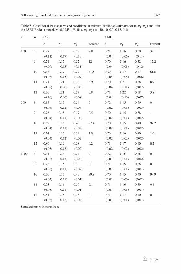
Self-exciting threshold binomial autoregressive processes 397
Table 7 Conditional least squares and conditional maximum likelihood estimates for (r, π1, π2) and R inthe LSET-BAR(1) model. Model M3: (N , R; r, π1, π2) = (40, 10; 0.7, 0.15, 0.4)T R CLS CML
r π1 π2 Percent r π1 π2 Percent
100 8 0.77 0.18 0.28 2.8 0.71 0.16 0.30 3.6
(0.11) (0.07) (0.13) (0.04) (0.06) (0.11)
9 0.71 0.17 0.32 12 0.70 0.16 0.32 12.2
(0.09) (0.05) (0.11) (0.04) (0.05) (0.12)
10 0.66 0.17 0.37 61.5 0.69 0.17 0.37 61.5
(0.08) (0.05) (0.07) (0.05) (0.05) (0.08)
11 0.71 0.21 0.38 8.9 0.70 0.21 0.38 8.9
(0.09) (0.10) (0.06) (0.04) (0.11) (0.07)
12 0.76 0.21 0.37 3.8 0.71 0.22 0.38 3.8
(0.10) (0.10) (0.08) (0.04) (0.10) (0.07)
500 8 0.83 0.17 0.34 0 0.72 0.15 0.36 0
(0.05) (0.02) (0.05) (0.02) (0.01) (0.03)
9 0.76 0.15 0.37 0.5 0.70 0.15 0.38 1
(0.04) (0.01) (0.03) (0.02) (0.01) (0.02)
10 0.69 0.15 0.40 97.4 0.70 0.15 0.40 97.2
(0.04) (0.01) (0.02) (0.02) (0.01) (0.02)
11 0.74 0.16 0.39 1.9 0.70 0.16 0.40 1.6
(0.04) (0.02) (0.02) (0.02) (0.02) (0.02)
12 0.80 0.19 0.38 0.2 0.71 0.17 0.40 0.2
(0.05) (0.03) (0.02) (0.02) (0.02) (0.02)
1000 8 0.84 0.16 0.34 0 0.72 0.15 0.36 0
(0.03) (0.03) (0.03) (0.01) (0.01) (0.02)
9 0.76 0.15 0.38 0 0.71 0.15 0.38 0
(0.03) (0.01) (0.02) (0.01) (0.01) (0.01)
10 0.70 0.15 0.40 99.9 0.70 0.15 0.40 99.9
(0.02) (0.01) (0.01) (0.01) (0.00) (0.02)
11 0.75 0.16 0.39 0.1 0.71 0.16 0.39 0.1
(0.03) (0.01) (0.01) (0.01) (0.01) (0.01)
12 0.81 0.18 0.38 0 0.71 0.17 0.40 0
(0.03) (0.02) (0.02) (0.01) (0.01) (0.01)
Standard errors in parentheses
123

398 T. A. Möller et al.
Table 8 Conditional least squares and conditional maximum likelihood estimates for (r, π1, π2) and R inthe LSET-BAR(1) model. Model M4: (N , R; r, π1, π2) = (20, 5; 0.7, 0.15, 0.4)T R CLS CML
r π1 π2 Percent r π1 π2 Percent
100 3 0.82 0.23 0.24 6.5 0.73 0.17 0.27 3.1
(0.10) (0.14) (0.10) (0.04) (0.05) (0.09)
4 0.75 0.17 0.29 1.1 0.71 0.16 0.31 7.8
(0.10) (0.05) (0.10) (0.05) (0.03) (0.10)
5 0.65 0.16 0.37 68.9 0.69 0.16 0.37 74.8
(0.09) (0.03) (0.07) (0.04) (0.05) (0.09)
6 0.76 0.21 0.34 9.9 0.71 0.19 0.36 9.8
(0.09) (0.08) (0.10) (0.04) (0.05) (0.09)
7 0.82 0.24 0.29 3.9 0.73 0.21 0.35 4.5
(0.08) (0.10) (0.12) (0.04) (0.06) (0.10)
500 3 0.90 0.28 0.19 0 0.73 0.16 0.29 0
(0.03) (0.14) (0.16) (0.02) (0.01) (0.04)
4 0.81 0.17 0.32 0 0.71 0.15 0.04 0
(0.04) (0.02) (0.05) (0.02) (0.01) (0.03)
5 0.69 0.15 0.40 99.5 0.70 0.15 0.40 99.9
(0.04) (0.01) (0.02) (0.02) (0.01) (0.02)
6 0.80 0.19 0.37 0.4 0.71 0.17 0.39 0.1
(0.04) (0.03) (0.04) (0.02) (0.02) (0.02)
7 0.88 0.24 0.26 0.1 0.73 0.19 0.39 0
(0.04) (0.13) (0.34) (0.02) (0.02) (0.03)
1000 3 0.90 0.27 0.20 0 0.74 0.16 0.30 0
(0.02) (0.05) (0.08) (0.01) (0.01) (0.03)
4 0.82 0.17 0.32 0 0.71 0.15 0.3 0
(0.03) (0.01) (0.03) (0.01) (0.01) (0.02)
5 0.69 0.15 0.40 99.9 0.70 0.15 0.40 99.9
(0.02) (0.01) (0.01) (0.01) (0.01) (0.01)
6 0.80 0.18 0.37 0.1 0.71 0.17 0.40 0.1
(0.03) (0.02) (0.02) (0.01) (0.01) (0.01)
7 0.88 0.23 0.26 0 0.73 0.19 0.39 0
(0.03) (0.04) (0.08) (0.01) (0.02) (0.02)
Standard errors in parentheses
123
Self-exciting threshold binomial autoregressive processes 399
References
Billingsley, P.: Statistical Inference for Markov Processes. Statistical Research Monographs. University ofChicago Press, Chicago (1961)
Chan, K.S., Tong, H.: On the use of the deterministic Lyapunov function for the ergodicity of stochasticdifference equations. Adv. Appl. Probab. 17, 666–678 (1985)
Chan, K.S., Petruccelli, J.D., Tong, H.,Woolford, S.W.: Amultiple-thresholdAR(1)model. J. Appl. Probab.22, 267–279 (1985)
Chan, W.S., Wong, A.C.S., Tong, H.: Some nonlinear threshold autoregressive time series models foractuarial use. N. Am. Actuar. J. 8, 37–61 (2004). doi:10.1080/10920277.2004.10596170
Chan, K.S., Li, D., Ling, S., Tong, H.: On conditionally heteroscedastic AR models with thresholds. Stat.Sin. 24(2), 625–652 (2014)
Chen, C.W.S., So, M.K.P., Liu, F.C.: A review of threshold time series models in finance. Stat. Interface 4,167–182 (2011)
Cline, D.B.H., Pu, H.H.: Stability of nonlinear AR(1) time series with delay. Stoch. Processes Appl. 82,307–333 (1999)
Cline, D.B.H., Pu, H.H.: Stability and the Lyapounov exponent of threshold AR-ARCHmodels. Ann. Appl.Probab. 14, 1920–1949 (2004)
Corradi,V., Swanson,N.R.: Predictive density and conditional confidence interval accuracy tests. J. Econom.135(1–2), 187–228 (2006)
Hansen, B.E.: Threshold autoregression in economics. Stat. Interface 4, 123–127 (2011)Klimko, L.A., Nelson, P.I.: On conditional least squares estimation for stochastic processes. Ann. Stat. 6,
629–642 (1978)Lanne,M., Saikkonen, P.: Non-linearGARCHmodels for highly persistent volatility. Econom. J. 8, 251–276
(2005)Liebscher, E.: Towards a unified approach for proving geometric ergodicity and mixing properties of non-
linear autoregressive processes. J. Time Ser. Anal. 26, 669–689 (2005)McKenzie, E.: Some simplemodels for discrete variate time series.Water Resour. Bull. 21, 645–650 (1985).
doi:10.1111/j.1752-1688.1985.tb05379.xMöller, T., Weiß, C.H.: Threshold models for integer-valued time series with infinite or finite range. In:
Steland, A., Rafajłowicz, E., Szajowski, K. (eds.) StochasticModels, Statistics and Their Applications,Springer Proceedings in Mathematics & Statistics, vol. 122, Springer, Berlin, pp. 327–334 (2015).doi:10.1007/978-3-319-13881-7_36
Monteiro, M., Scotto, M.G., Pereira, I.: Integer-valued self-exciting threshold autoregressive processes.Commun. Stat. Theory Methods 41, 2717–2737 (2012)
Petruccelli, J.D.: A comparison of tests for setar-type non-linearity in time series. J. Forecast. 9(1), 25–36(1990). doi:10.1002/for.3980090104
Robert-Koch-Institut: Robert-Koch-Institut: SurvStat@RKI. http://www3.rki.de/SurvStat. Accessed 2014-07-02 (2014)
Samia, N.I., Chan, K.S., Stenseth, N.C.: A generalized threshold mixed model for analyzing nonnormalnonlinear time series, with application to plague in Kazakhstan. Biometrika 94(1), 101–118 (2007).doi:10.1093/biomet/asm006
Scotto, M., Weiß, C.H., Silva, M.E., Pereira, I.: Bivariate binomial autoregressive models. J. Multivar. Anal.125, 233–251 (2014)
Stenseth, N.C., Samia, N.I., Viljugrein, H., Kausrud, K.L., Begon, M., Davis, S., Leirs, H., Dubyanskiy,V.M., Esper, J., Ageyev, V.S., Klassovskiy, N.L., Pole, S.B., Chan, K.S.: Plague dynamics are drivenby climate variation. In: Proceedings of the National Academy of Sciences, vol. 103, pp. 13110–13115(2006). doi:10.1073/pnas.0602447103, http://www.pnas.org/content/103/35/13110.full.pdf+html
Steutel, F.W., van Harn, K.: Discrete analogues of self-decomposability and stability. Ann. Probab. 7,893–899 (1979)
Thyregod, P., Carstensen, J., Madsen, H., Arnbjerg-Nielsen, K.: Integer valued autoregressive mod-els for tipping bucket rainfall measurements. Environmetrics 10(4), 395–411 (1999). doi:10.1002/(SICI)1099-095X(199907/08)10:4<395:AID-ENV364>3.0.CO;2-M
Tong, H.: Threshold models in non-linear time series analysis. Lecture Notes in Statistics, vol. 21. Springer(1983)
Tong, H.: Non-linear Time Series. A Dynamical System Approach. Clarendon Press, Oxford (1990)Tong, H.: Threshold models in time series analysis—30 years on. Stat. Interface 4, 107–118 (2011)
123
400 T. A. Möller et al.
Tong, H., Lim, K.S.: Threshold autoregression, limit cycles and cyclical data. J. R. Stat. Soci. Ser. B 42,245–292 (1980)
Turkman, K.F., Scotto, M.G., de Zea, Bermudez P.: Non-linear Time Series: Extreme Events and IntegerValue Problems. Springer, Basel (2014)
Wang, C., Liu, H., Yao, J.F., Davis, R.A., Li, W.K.: Self-excited threshold Poisson autoregression. J. Am.Stat. Assoc. 109, 777–787 (2014). doi:10.1080/01621459.2013.872994
Weiß, C.H.: A new class of autoregressive models for time series of binomial counts. Commun. Stat. TheoryMethods 38(4), 447–460 (2009). doi:10.1080/03610920802233937
Weiß, C.H., Kim, H.Y.: Parameter estimation for binomial AR(1) models with applications in finance andindustry. Stat. Pap. 54, 563–590 (2013)
Weiß, C.H., Kim,H.Y.: Diagnosing andmodeling extra-binomial variation for time-dependent counts. Appl.Stoch. Models Bus. Ind. 30, 588–608 (2014). doi:10.1002/asmb.2005
Weiß, C.H., Pollett, P.K.: Binomial autoregressive processes with density-dependent thinning. J. Time Ser.Anal. 35, 115–132 (2014)
Yu, K., Zou, H., Shi, D.: Integer-valued moving average models with structural changes. Math. ProblemsEng. Article ID 231592 (2014)
Zou, H., Yu, K.: First order threshold integer-valued moving average processes. Dyn. Contin. DiscreteImpuls. Syst. Ser. B Appl. Algorithms 21, 197–205 (2014)
Zucchini,W.,MacDonald, I.L.:HiddenMarkovModels for TimeSeries:An IntroductionUsingR.Chapman& Hall/CRC Monographs on Statistics & Applied Probability. CRC Press, Boca Raton (2009)
123