repository productivity at the post

Productivity at the Post: its Drivers and its Distr ibution

E. Grifell - Tatjé C.A.K. Lovell

Abstract

We study the productivity, financial and distributional performance of the United States Postal Service subsequent to its 1971 reorganization. We investigate the magnitude and the economic drivers of productivity change (technical change, change in cost efficiency, and scale economies), and we investigate the distribution of the financial benefits of productivity change (among consumers of postal services, postal employees and other resource suppliers, and residual claimants). We find improvements in technology to have been the main driver of, and diseconomies of scale to have been the main drag on, productivity change. We find labor to have been the main beneficiary, and consumers of postal services the main losers, from postal reorganization.

This is a postprint version of the article that was published in

Grifell – Tatjé, E. and C.A.K. Lovell (2008), “Productivity at the Post: its Drivers and its Distribution,” Journal of Regulatory Economics vol.33, issue 2, April, pp 133 – 158. DOI: 10.1007/s11149-007-9051-y JEL codes : C60, D24, D33, L32 Keywords : productivity, profit, distribution, postal service

Corresponding author: E. Grifell-Tatjé Universitat Autònoma de Barcelona, Departament d’Economia de l’Empresa, Edifici B – Campus de la UAB, 08193 Bellaterra (Cerdanyola de Vallés), Barcelona. Spain. email: [email protected] phone +34 93 581 2251; fax +34 93 581 2555. C.A.K. Lovell University of Georgia and University of Queensland, School of Economics, Colin Clark Building, St Lucia, Brisbane, QLD 4072. Australia. email: [email protected]

Grifell – Tatjé, E. and C.A.K. Lovell (2008), “Productivity at the Post: its Drivers and its Distribution,” Journal of Regulatory Economics vol.33, issue 2, April, pp 133 – 158. DOI: 10.1007/s11149-007-9051-y

1

Productivity at the Post: its Drivers and its Dist ribution ∗∗∗∗

1. Introduction

We study the productivity, financial and distributional performance of the United States Postal Service (USPS) subsequent to its 1971 reorganization from the Post Office Department (POD) to an independent government agency. The reorganization preserved the monopoly powers originally granted to the POD (the “private express statutes”), as well as the universal service at uniform price requirement, and so the USPS remains a regulated public monopoly. However its operating environment has changed in ways that could not have been foreseen nearly four decades ago. The population shift to the south and west has stretched its delivery network. Increased competition for overnight and package delivery services has eroded its customer base. New technologies such as facsimile, electronic mail, the internet and automatic bill payment systems have further eroded its customer base. Thus its monopoly powers notwithstanding, the USPS has operated in a rapidly changing market environment constrained (or protected) by an aging regulatory framework.

Although its growth has slowed recently, and even reversed in some service categories, the USPS remains a very large organization. It incurs nearly $72 billion in operating expense, roughly 80% of which is compensation and benefits for its nearly 800,000 employees. It generates over $72 billion in operating revenue, providing postal services to over 146 million delivery points. In light of its size and its omnipresence, its productivity performance (which we define as total factor productivity), its financial performance (which we define as operating profit), and the way it distributes the financial benefits of its productivity change to its various stakeholders, are all worthy of investigation.

These three issues would be of interest for an equally large and omnipresent unregulated, privately owned, profit seeking, publicly traded firm. With sufficiently strong competition in resource and product markets, one would expect the financial benefits of productivity change to be shared by its customers and its stockholders, the legally designated residual claimants. In a less competitive environment, one might expect a share of the financial benefits of productivity change to be captured by labor or other resource suppliers, with these additional expenses being passed along to customers in the form of price increases.

However the USPS is a regulated public monopoly, with uncertain economic objective(s) and lacking a regulator with any real ability to enforce financial discipline. The lack of serious competition from the private sector weakens the incentive for strong productivity performance. It also leads to the expectation of financial performance that reflects a weak opposition to resource price increases that, depending on the economic objective(s) of USPS and on the nature of


2

consumer demand elasticities for postal services, are passed along in the form of rate increases. Importantly, this expected financial transfer from consumers to resource suppliers is expected to occur independently of the nature of productivity performance. Each of these expectations is reinforced by the lack of a strong regulator. However the most interesting feature of public ownership is the nature of income distribution in the absence of a clearly identifiable residual claimant group to reap the financial benefits of productivity change. The absence of stockholders as legally designated residual claimants raises the issue of what group, if any, constitutes a de facto residual claimant group. Labor is the most, perhaps the only, organized resource supplier at USPS, which leads to the expectation that the financial transfer goes from consumers primarily to labor rather than to all resource suppliers. These features all combine to make the relationships among productivity, profit and income distribution particularly significant issues at USPS.

Surprisingly little research has been devoted to the performance of the USPS. Much of what is available is concerned with various reform proposals aimed at improving its performance. These include the potential for revenue cap regulation, the role of the universal service and uniform price obligations, the growth of worksharing and competing forms of communication, and the prospects for partial or complete privatization. The President’s Commission on the United States Postal Service (2003) has recommended reforms that address some of these issues, and bills remain pending in Congress as of late 2006. It is particularly noteworthy that productivity change, surely an essential component of any conception of “performance,” has been largely ignored. The USPS does report its productivity performance, in terms of both output per workhour and total factor productivity, together with its financial performance, in terms of operating profit or loss, in its Annual Reports. In its three most recent Annual Reports the USPS claims that its 2003 – 2006 productivity growth “is equivalent to” $2.6 billion in expense reductions. However neither the economic drivers nor the financial consequences, including distributional impacts, of productivity change at the USPS have been systematically explored, either in the research community or by the USPS itself.1

We have three objectives. The first is to link productivity trends at the USPS with trends in its operating profit performance. The two need not move together, and the linkage between the two is forged by the relationship between trends in postal rates and input prices, which we refer to as price recovery. We use this linkage, and data provided by the USPS, to address the second and third objectives. The second objective is to explore the economic drivers of productivity change, which can be identified as change in the efficiency of resource allocation, improvements in technology, and change in the exploitation of scale economies. The third objective is perhaps the most interesting in light of the absence of a readily identifiable residual claimant group, and involves an investigation of the distribution of the financial benefits of productivity change,


3

which can be associated with consumers of postal services, postal employees and other resource suppliers, and the recipients of operating profit or loss.

Our analytical framework is built around a detailed decomposition of year-to-year change in operating profit at the USPS. Similar decompositions have been described by Davis (1955) as “productivity accounting,” and used by Kendrick and Creamer (1961) to analyze productivity, profit and income distribution at a number of US companies. Our application to time series data on a single public organization is similar to those of Denny et al. (1981), who explore the economic drivers (but not the distribution of the financial benefits) of productivity change at Bell Canada, and of Lawrence et al. (2006), who explore the distribution of the financial benefits (but not the economic drivers) of productivity growth at Telstra, Australia’s largest telecommunications firm. In both respects our framework is in the spirit of the French tradition as exemplified by Puiseux and Bernard (1965), who explore the economic drivers and the distributional impacts of productivity change at Electricité de France.

Our analytical framework differs from those used in the studies just cited. We employ superlative indicators of price and quantity change. However an exclusive reliance on indicators permits the identification of the sources and beneficiaries of productivity change by variable, but identification of the economic drivers of productivity change requires economic analysis. We therefore augment our superlative indicator approach by exploiting the economic theory of production, which enables us to uncover the economic drivers, as well as the distributional consequences, of productivity change at the USPS.

The paper unfolds as follows. Section 2 provides a brief background on reorganization and its consequences for productivity and financial performance at the USPS. The analytical framework we use to identify the drivers and beneficiaries of productivity change is developed in Section 3, where we also describe the empirical technique we use to implement the decomposition of change in operating profit from one year to the next. Section 4 provides a description of the USPS data, an aggregate time series of quantities and prices over the period 1963-2004. We describe the results of the empirical analysis in Section 5, where we identify the economic drivers and the distributional consequences of productivity change. Section 6 concludes with a summary of our findings and their implications for postal reform.

2. Background

In the 1960s, over a century after it became a Cabinet-level department, the POD was in economic and financial trouble. With inadequate capital investment and ineffective managerial control in a highly politicized operating environment, it was increasingly incapable of distributing growing volumes of mail through an expanding network. In addition, it was suffering from financial neglect, with high


4

labor costs and subsidized rates that bore little relation to costs. Annual operating losses in excess of a billion current dollars were common.2

In April 1967 President Johnson appointed a Commission on Postal Reorganization. In June 1968 the Commission recommended that the POD be reorganized as an independent agency within the executive branch of government, one that would be run like a business, financially self-sustaining and insulated from political pressure. Following protracted negotiations, the POD was transformed into the USPS with the passage of the Postal Reorganization Act (PRA), signed by President Nixon in August 1970. The USPS began operations July 1, 1971 as an independent agency of the executive branch.

The PRA transferred operational authority from Congress to an ostensibly independent regulator, the Postal Rate Commission (PRC). However the authority of the PRC is limited in a number of important ways, with unfortunate consequences.

(a) The PRC cannot set postal rates, but merely recommends rates that can be, and have been, overruled by the USPS Board of Governors. Limited oversight applies not just to rate increases, but also to cross-subsidy from monopolized to competitive service categories.

(b) The PRA established collective bargaining on wages and working conditions, with binding arbitration, and required postal worker wages and benefits to be comparable to those prevailing in similar occupations in the private sector. However it did not provide the PRC with an enforcement mechanism to ensure comparability, and it is widely believed that labor costs are higher at the USPS than at comparable occupations in the private sector, and that the gap has widened since reorganization.

(c) The USPS is exempt from SEC disclosure requirements, and the PRC is constrained by a lack of subpoena power in its ability to obtain information on USPS operations and finances. It is difficult to regulate in the dark.

(d) The PRA required the USPS to establish a break-even rate structure that covers direct and indirect costs attributable to each service category, plus a proportion of institutional costs. However the PRC has little influence over operating costs, which in turn limits its influence over postal rates. In prescient anticipation of future difficulties, the PRA provided for the recovery of operating losses through borrowing from the Department of Treasury’s Federal Financing Bank, as well as through future rate increases. Thus a potential candidate for the title of residual claimant is the Federal Financing Bank, which at the end of our study period held $1.8 billion of USPS long-term and short-term debt (down from $11.1 billion two years earlier). However the PRC cannot compel the USPS to return annual operating profits to the Bank, and so the Bank’s claims are unlikely to be enforceable and its candidacy for residual claimant status is not compelling.


5

(e) A natural candidate for the title of ultimate residual claimant to the operating profits of a public organization such as the USPS is the taxpayers. However their residual claims are neither enforceable nor transferable, leaving them with little incentive and no power to hold management accountable for the financial performance of the USPS. Property rights that are not enforceable and not transferable render taxpayers impotent recipients of annual profits or losses, rather than legally protected residual claimants. Moreover, since taxpayers are consumers of postal services, they become potential double victims of USPS financial performance.3

The PRA did not endow the PRC with sufficient regulatory authority to do its job. Against this background, the President’s Commission reform proposals address many of the inadequacies mentioned above, although four years on they remain proposals. The shortcomings of the current regulatory regime and the nature of the reforms proposed by the President’s Commission suggest several hypotheses about the productivity, financial and distributional performance of the USPS to date.

Weak PRC influence over labor costs, in conjunction with labor’s strong organization and the weak residual claimant rights of other groups, motivates the distributional hypothesis that postal employees have been big winners from reorganization. The PRA break-even mandate, to the extent that it is honored, requires losers as well as winners, and the second distributional hypothesis is that weak PRC influence over postal rates has made consumers of postal services big losers. The PRA recommendation that the USPS be “run like a business,” while not legally binding, nonetheless leads to a third distributional hypothesis, that operating losses have diminished subsequent to reorganization. However the PRA allowed the USPS access to the Federal Financing Bank, which leads to the expectation that operating losses would not be eliminated quickly. Whatever the speed, improved financial performance must come from somewhere. A hypothesis concerning the economic drivers of improved financial performance is that productivity improvements have been the main driving force behind improved financial performance. A corollary to the first hypothesis that labor has been a big winner asserts that productivity change has been biased, and that substitution away from postal employees has occurred, either through improved cost efficiency or through the adoption of new technologies, particularly of the labor saving kind. We explore each of these hypotheses in Section 5.

Productivity has improved since reorganization, although growth rates remain relatively low. Figure 1 tracks the USPS calculation of its cumulative total factor productivity over the period 1963-2004. The annual growth rate has trended upward, improving from 0.04% before reorganization to 0.5% since. USPS productivity was barely 17% higher in 2004 than it was at reorganization in 1972. To put these figures in perspective, in its Annual Reports the USPS benchmarks its productivity performance against that of the US private non-farm


6

business sector, as reported by the Bureau of Labor Statistics. The BLS (2007) reports annual growth rates of multifactor productivity of 1.0% over the period 1963-2004, slowing from 1.7% over the pre-reorganization period to 0.8% over the post-reorganization period. Productivity in the non-farm business sector was 29% higher in 2004 than it was in 1972. Although much of the divergence occurred prior to reorganization, since 1972 productivity growth at the USPS has remained barely half as fast as in the private non-farm business sector.

Insert Figure 1 about here.

These modest but accelerating rates of productivity growth have contributed to a substantial improvement in the bottom line. Table 2 tracks annual operating profit, in current dollars, over the 1963-2004 period. Mean annual operating losses mounted through 1976, bottoming out at $2.6 billion. Losses then diminished through 1991 and turned to operating profit through most of the period since 1992. Although productivity growth has contributed to the remarkable turnaround in the financial performance of the USPS, it is clear from Figures 1 and 2 that there must be more to the story. Trends in resource prices and postal rates have played an important role as well, as our analysis will demonstrate.


3. The Analytical Framework

Testing the hypotheses developed in Section 2 requires an analytical framework, which we develop in Sections 3.1 and 3.2, and an estimation procedure, which we develop in Section 3.3. The analytical framework is an extension of that developed by Grifell-Tatjé and Lovell (1999), and revolves around change in operating profit from one fiscal year to the next. This does not imply that we assign to USPS the economic objective of profit maximization. We have noted the “uncertain economic objective(s)” of USPS, and we have emphasized the lack of credible residual claimants to impose an economic objective on USPS. We remain agnostic concerning what motivates managerial decision-making at USPS. We use operating profit as a metric because of the prominence accorded it in USPS annual reports, because it provides a valid indicator of financial performance, of the financial consequences of the pursuit of whatever economic objective the USPS does pursue, and because it provides a convenient analytical framework for quantifying the economic drivers and the financial and distributional consequences of productivity change at USPS.4

3.1 Decomposing Change in Operating Profit


7

We begin with an expression for operating profit in period t,

πt = Rt – Ct = ptyt – Σnwntxn

t, (1)

where π is operating profit, R is revenue, C is cost, p is the price of output y and wn is the price of input xn, n=1,…,N.5

Operating profit changes through time because quantities change and because prices change. We decompose the change in operating profit between periods t and t+1 (πt+1 - πt) into an aggregate quantity effect and an aggregate price effect. We avoid having to choose between base period and comparison period weights by using arithmetic mean price weights ( p and w n) and arithmetic mean quantity weights ( y and x n) to generate

πt+1 - πt = [ p (yt+1 - yt) – Σ w n(xnt+1 - xn

t)] + [( y (pt+1 - pt) – Σ x n(wnt+1 - wn

t)], (2)

which decomposes profit change into the contributions of changes in individual quantities, holding prices fixed at arithmetic mean values, and changes in individual prices, holding quantities fixed at arithmetic mean values. Because profit change is expressed in value terms, so is each component.

The first term on the right side of (2) is an aggregate quantity effect that shows the contribution of (1+N) individual quantity changes to profit change, holding (1+N) prices fixed at their arithmetic mean values p = (½)(pt + pt+1) and w n = (½)(wn

t + wnt+1). The (1+N) components of the aggregate quantity effect are

Bennet (1920) quantity indicators. The second term on the right side is an aggregate price effect that shows the contribution of (1+N) individual price changes to profit change, holding (1+N) quantities fixed at their arithmetic mean values y = (½)(yt + yt+1) and x n = (½)(xn

t + xnt+1). The (1+N) components of the

aggregate price effect are Bennet price indicators. While the more familiar quantity and price indexes express changes as pure numbers in ratio form, quantity and price indicators express changes in monetary units in difference form.6

Expression (2) identifies the individual prices and quantities responsible for profit change. It is also useful to identify the beneficiaries of the fruits of productivity change. This can be accomplished by rearranging (2) to obtain

[ p (yt+1 - yt) – Σ w n(xnt+1 - xn

t)] = (πt+1 - πt) – y (pt+1 - pt) + Σ x n(wnt+1 - wn

t). (3)

The left side is the aggregate quantity effect from (2). The right side quantifies the gains or losses of the individual recipients of the benefits of the quantity effect. The recipients include members of whatever group to which the


8

change in operating profit (πt+1 - πt) is allocated, consumers of postal services who pay the change in output price, with pt+1 < pt ⇒ - y (pt+1 - pt) > 0, and individual resource suppliers who receive the changes in individual resource prices, with wn

t+1 > wnt ⇒ x n(wn

t+1 - wnt) > 0, n=1,…,N.

3.2 Decomposing the Quantity Effect

The right side of (3) identifies the recipients of the benefits of the quantity effect, and quantifies their receipts. The left side, the quantity effect itself, identifies the agents responsible for the quantity effect, and quantifies their contributions. Both decompositions are based on observed data and superlative indicators. Together they constitute what Davis (1955) called productivity accounting. However decomposing the quantity effect into its economic drivers, as distinct from its responsible agents, requires economic analysis.

Tt and Tt+1 in Figure 3 are sets of feasible production activities in periods t and t+1, and Lt(yt), Lt+1(yt) and Lt+1(yt+1) in Figure 4 are input sets corresponding to Tt and Tt+1. In Figure 3 Tt ⊂ Tt+1 on the assumption that technical progress has occurred. The same assumption generates Lt(yt) ⊂ Lt+1(yt) in Figure 4, in which Lt+1(yt+1) ⊂ Lt+1(yt) on the assumption that yt+1 > yt. In both Figures the objective is to decompose the change from (xt,yt) to (xt+1,yt+1), which when weighted by arithmetic mean prices is the quantity effect on the left side of (3).

In both Figures xCEt and xCE

t+1 are cost-efficient input vectors for (yt,wt,Tt) and (yt+1,wt+1,Tt+1) respectively, that purge xt and xt+1 of cost inefficiency in resource use. In addition, improvements in technology between periods t and t+1 enable cost-efficient input vector xCE

t to be displaced by input vector xE, which is cost-efficient for (yt,wt,Tt+1). The three cost minimizing input vectors xCE

t, xCEt+1

and xE are unobserved. Identifying them enables us to identify the contributions to the quantity effect of a change in cost efficiency, by comparing (xt+1 - xCE

t+1) with (xt - xCE

t); an improvement in technology, represented by (xCEt - xE); and the

exploitation of scale economies reflected in a movement along the surface of Tt+1 from (yt,xE) to (yt+1,xCE

t+1). These three sources comprise a productivity effect, which is one component of the aggregate quantity effect on the left side of (3).



The quantity effect is often equated with a productivity effect. However this is not necessarily the case, since the quantity effect has a margin component as well as a productivity component, as evidenced by the decomposition


9

p (yt+1 - yt) – Σ w n(xnt+1 - xn

t) quantity effect

= [ p - (Σ w nxnCEt)/yt](yt+1 - yt) margin effect

+ (Σ w nxnCEt/yt)(yt+1 - yt) – Σ w n(xn

t+1 - xnt) productivity effect (4)

The quantity effect collapses to a productivity effect only if the margin effect is zero. For nonzero output change the margin effect is zero if the margin [ p -

(Σ w nxnCEt)/yt] = 0. The margin effect expresses the simple idea that expansion

with a positive margin is profitable, quite independently of any improvement in productivity. The margin effect is expressed in value terms, and weights output change by the margin between arithmetic mean output price and cost-efficient average cost evaluated at arithmetic mean input prices. Expansion with a positive cost-efficient margin [ p - (Σ w nxnCE

t)/yt > 0] contributes positively to the quantity effect, and hence to profit change. Conversely, a negative cost-efficient margin signals that arithmetic mean output price is insufficient to cover cost-efficient average cost, much less actual average cost, and contraction would reduce losses. We show below that the post-reorganization performance of the USPS illustrates both possibilities.7

The productivity effect also is expressed in value terms, as the difference between weighted output change and weighted input change. The weight on output change is cost-efficient average cost. The productivity effect decomposes as

Σ w n(xnCEt/yt)(yt+1 - yt) – Σ w n(xn

t+1 - xnt) productivity effect

= [Σ w n(xnt - xnCE

t) – Σ w n(xnt+1 - xnCE

t+1)] cost efficiency effect

+ [Σ w n(xnCEt - xnE)] technical change effect

+ Σ w n(xnCEt/yt)(yt+1 - yt) - Σ w n(xnCE

t+1 - xnE) scale effect (5)

The cost efficiency effect captures the contribution to the productivity effect of a change in the cost efficiency of resource allocation between periods t and t+1, by comparing the value of (xt+1 - xCE

t+1) with that of (xt - xCEt), using arithmetic

mean input price weights. A positive cost efficiency effect measures the financial benefits of an improvement in cost efficiency, which contributes positively to the productivity effect and enhances profit change.

The technical change effect captures the contribution to productivity change of an improvement in technology between periods t and t+1, evaluated with an input-saving orientation at yt, by comparing the cost of xCE

t on the surface of Tt with that of xE on the surface of Tt+1, again using arithmetic mean input price


10

weights. A positive technical change effect measures the financial benefits of cost-saving technical progress, which contributes positively to the productivity effect and enhances profit change. As Figure 4 indicates, technical change can be biased.

The scale effect corresponds to a movement along the surface of Tt+1 from (yt,xE) to (yt+1,xCE

t+1), and captures the contribution of scale economies to the productivity effect. A positive scale effect reflects either expansion in the presence of increasing returns to scale, or contraction in the presence of decreasing returns to scale, either of which contributes positively to the quantity effect and enhances profit change.8,9

3.3 Implementing the Decomposition of the Quantity Effect

In decompositions (4) and (5) the output quantity y and the input quantity vector x are observed, as is the input price vector w. However the cost-efficient input quantity vectors xCE and xE are not observed, and as Figures 3 and 4 suggest they must be retrieved from observed data and the technologies. However because the technologies are unobserved as well, we use a sequential form of data envelopment analysis (DEA) to approximate them. This enables us to solve for the cost-efficient input quantity vectors xCE and xE.

Since xCEt is a cost minimizing input vector for (yt,wt,Tt), it can be identified

as the solution to the linear program

minx {wtTx : x ≧ Xtλ, Ytλ ≧ yt, λ ≧ 0, ∑λ= 1}. (6)

In this program the objective is to find an input quantity vector x that minimizes expenditure wtTx = ∑wn

txnt required to produce yt, provided that (x,yt) is

feasible with Tt. The data matrices Yt and Xt contain all outputs and inputs observed in periods {1,…,t}. Thus feasibility of (x,yt) requires that (x,yt) belong to

the production set TtDEA = {(x,yt) : x ≧ Xtλ, Ytλ ≧ yt, λ ≧ 0, ∑λ= 1}. Tt

DEA is the DEA approximation to the unobserved production set Tt. Tt

DEA is constructed sequentially, on the assumption that activities adopted in previous years are remembered and remain available for adoption in subsequent years; this

assumption rules out technical regress. The convexity constraint {λ ≧ 0, ∑λ = 1} allows the surface of Tt

DEA to satisfy variable returns to scale. The solution to this program is the cost-efficient input quantity vector xCE

t in Figures 3 and 4 and in decompositions (4) and (5).

Since xE is the solution to the same cost minimizing problem, but using technology Tt+1, solving for xE requires expanding the data matrices to Xt+1 and Yt+1 and retaining wt and yt. The solution to this program is the cost-efficient input quantity vector xE in Figures 3 and 4 and in decompositions (4) and (5).


11

Once the annual cost-efficient input quantity vectors xCE and xE are calculated, they are inserted into decomposition (4) to quantify the margin effect and the productivity effect. The sources of productivity change are quantified on the right side of (5), and the beneficiaries of productivity change are quantified on the right side of (3). The input quantity vectors are identified using observed input prices, and their effects are quantified using arithmetic mean input prices.

4. Data

Our database is a 1963-2004 time series. Although we utilize the entire time series in sequential DEA to construct annual technologies, we restrict our empirical analysis to the post-reorganization period 1972-2004. Thus in our empirical analysis t=1 corresponds to the year 1972, with 1972 technology T1

DEA constructed sequentially from 1963-1972 data, t=2 corresponds to the year 1973, with 1973 technology T2

DEA constructed sequentially from 1963-1973 data, and so on. This enables us to focus on the performance of the USPS, and not that of its predecessor POD.10

We divide the post-reorganization period into three decades and a terminal era, inspired by trends in operating profit depicted in Figure 2. The first, 1972-1982, plumbs the financial depths. The second, 1982-1992, tracks shrinking losses that turned to the first year of operating profit in 1992. The third, 1992-2001, was a generally profitable decade. The terminal era, 2001-2004, begins with the general business slowdown following the 9/11/01 terrorist attacks and the anthrax attacks at post offices, and it also marks the beginning of the term of the current Postmaster General.

With one exception, all variables are contained in an internal database the USPS has provided to us. The exception is operating revenue R, which is obtained from USPS annual reports. Operating revenue is expressed in current dollars, and excludes the general public service subsidy and the foregone revenue appropriation because neither reflects revenue from operations. The two excluded items have declined from 18% of total revenue in 1972 to 0.05% of total revenue in 2004.

Operating cost C is the sum of expenditures on capital, labor and materials inputs, and also is expressed in current dollars. The operating profit series is defined as π = R - C and is depicted in Figure 2.11

The output quantity index y is a convex combination of a mail quantity index and a delivery network index, the former incorporating seven mail categories and four miscellaneous services and the latter combining urban and rural delivery points. An output price index is defined as p = R/y and set to unity in 1972, with the output quantity index expressed in 1972 dollars.

Quantity and price indexes for capital, labor and materials are defined in the same way, with input price indexes set to unity in 1972 and input quantity


12

indexes expressed in 1972 dollars. These indexes incorporate seven, 12 and 29 categories, respectively.

The data are summarized, by sub-period, in Table 1. Certain trends are clear, although sub-period means and growth rates conceal considerable year-to-year variability in some variables. With this in mind, mean operating losses increased by 7.8% annually prior to reorganization, and declined by 10% annually thereafter. The impressive post-reorganization improvement in financial performance is clear from Table 1, as are the trends in individual quantities and prices. However the contributions of these trends to improved financial performance require indicators and analysis. In the next Section we use the analytical framework and estimation procedure developed in Section 3 to quantify the economic drivers and the individual beneficiaries of productivity change at USPS.

5. Results

Tables 2 – 4 are based on price and quantity indicators developed in Section 3.1, and convert price and quantity trends summarized in Table 1 into monetary contributions of price and quantity changes to profit change at USPS. Table 5 is based on the analytical framework developed in Section 3.2, and quantifies the economic drivers of productivity change at USPS. Like Table 1, Tables 2 – 5 report changes averaged over sub-periods, and these average changes conceal considerable variability in year-to-year changes for some indicators. 12

Table 2 is organized around decomposition (2), which allocates profit change to price change and quantity change. Over the entire post-reorganization period operating profit increased by nearly $120 million annually, despite unfavorable price trends that deteriorated from small positive contributions in the first two sub-periods to large negative contributions thereafter, and exerted a drag on operating profit of nearly $100 million annually. Both trends magnified after 2001. Operating profit in that subperiod increased by nearly $900 million annually, despite a continuing deterioration in the price structure that drained $265 million annually. We explore the very large favorable quantity effect in Table 3.

Table 3 also is organized around decomposition (2), and quantifies the contribution of each variable to quantity change. For the subperiod prior to 2001, the mean value of output growth exceeded the value of input growth (obtained by adding the capital, labor and materials quantity effects), generating, on average, a positive and growing contribution of the quantity effect to profit change. The situation changed dramatically after 2001. In that subperiod, the positive quantity effect magnified, contributing over $1.1 billion annually to profit change, despite an unprecedented mean decline in output that drained more than $250 million annually from the quantity effect. A positive quantity effect in the presence of a


13

negative output quantity effect requires a larger negative input quantity effect. Most of the negative input quantity effect can be traced to labor shedding, which contributed nearly $1.4 billion annually to the quantity effect, and to a reduction in complementary materials use that saved a lesser amount. We explore labor shedding further in Table 5.

It is noteworthy that expansion contributed positively to profit change prior to 2001, and contraction also contributed positively to profit change subsequently. Output contraction was largely exogenous, brought on by economic stagnation following the events of 2001, and by consumer substitution into alternative forms of communication. However the input contraction that made this output contraction profitable was endogenous and not guaranteed, and required good management. We refer to this period as one of “managing decline,” largely through reductions in the USPS workforce.

Table 4 is organized around decomposition (3), and provides an alternative decomposition of the quantity effect, in an effort to quantify the financial gains of the winners and the financial losses of the losers since reorganization. Throughout the entire post-reorganization period two groups, postal employees and consumers of postal services, dominated the positive and growing quantity effect. Suppliers of materials and, to a lesser extent, suppliers of capital services were modest nominal gainers, with gains of the latter depressed by low interest rates beginning in the 1990s. The Federal Financing Bank and taxpayers were also modest gainers (if $120 million annually can be called modest), in the sense that annual operating losses declined and finally turned to operating profit, some of which was returned to the Bank. However all of these gains were dominated, on average by one and two orders of magnitude, by the gains of postal employees, whose rising compensation drained over $1.3 billion annually from USPS operating profit. These gains were funded by the only losers since postal reorganization, postal customers. Since reorganization the USPS has transferred over $1.3 billion annually from its customers to its employees. These findings confirm and quantify the distributional hypotheses put forth in Section 2. However unlike the dramatic changes beginning in 2001 noted in Tables 2 and 3, this redistribution process was impervious to change. The average losses incurred by suppliers of capital services expanded, as did the gains accruing to the Federal Financing Bank and taxpayers, but the transfer of over $1.3 billion annually from postal customers to postal employees continued despite the downturn. Managing decline did not involve managing employee compensation or postal rates.

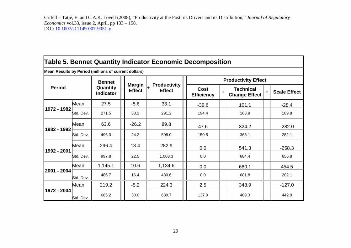
Table 5 provides an alternative decomposition of the quantity effect, built around decompositions (4) and (5), both of which augment raw data with economic analysis. The first objective is to quantify the contribution of productivity change to quantity change, and hence to profit change. This is accomplished in the first three columns, which implement decomposition (4) by decomposing the quantity effect into margin and productivity effects. Throughout the post-reorganization period the margin effect has been negative on average


14

and relatively small, suggesting that postal rates have not quite managed to cover cost-efficient average cost. It follows that postal rates have not covered actual average cost, and this explains why operating profit has been negative on average, although the upward trend in the margin effect is consistent with the upward trend in operating profit depicted in Figure 2. However in this exercise the USPS establishes its own best practice technology, so the benchmark “cost-efficient average cost” should be interpreted accordingly.

Throughout the post-reorganization period, the productivity effect has, on average, dominated the margin effect by two orders of magnitude. The productivity effect has delivered mean cost savings of $224 million annually, and its contribution has increased through successive sub-periods. Since 2001 productivity gains have reduced operating expenses by over $1 billion annually. This finding confirms and quantifies the hypothesis that productivity growth has been the primary source of improvement in financial performance at USPS.13

The productivity effect in Table 5 is cumulated over time in Figure 5. A comparison of the cumulative productivity effect in Figure 5 with the USPS cumulative total factor productivity index in Figure 1 reveals that the two follow precisely the same pattern throughout the post-reorganization period, with peaks and troughs in the same years. The only difference between the two Figures is the vertical axis, with productivity gains reported in Figure 1 as a cumulative index number and in Figure 5 as a cumulative contribution to the bottom line. We have made no use of the USPS total factor productivity series in our analysis, and we have obtained a productivity effect that behaves in exactly the same way.


The second objective of Table 5 is to quantify the contributions of the economic drivers of productivity change to profit change. This is accomplished in the final three columns, which implement decomposition (5).

The cost efficiency of resource allocation has not improved since reorganization, and has made virtually no contribution to productivity change, and hence to profit change. Again recalling that the USPS establishes its own best practice standards, it is not possible to discern whether this is due to persistent cost efficiency or to persistent resource misallocation. This finding contradicts the hypothesis of improvements in cost efficiency. It is, however, a predictable consequence of the limited ability of the PRC to regulate postal rates, which in turn offers the USPS little incentive to control operating costs. It is also consistent with political and labor opposition to streamlining the delivery network and to the introduction of new mail sorting technologies.

The primary driver of productivity change has been improvements in technology, which have delivered cost savings of nearly $350 million annually, and the average value of these savings has increased through successive sub-


15

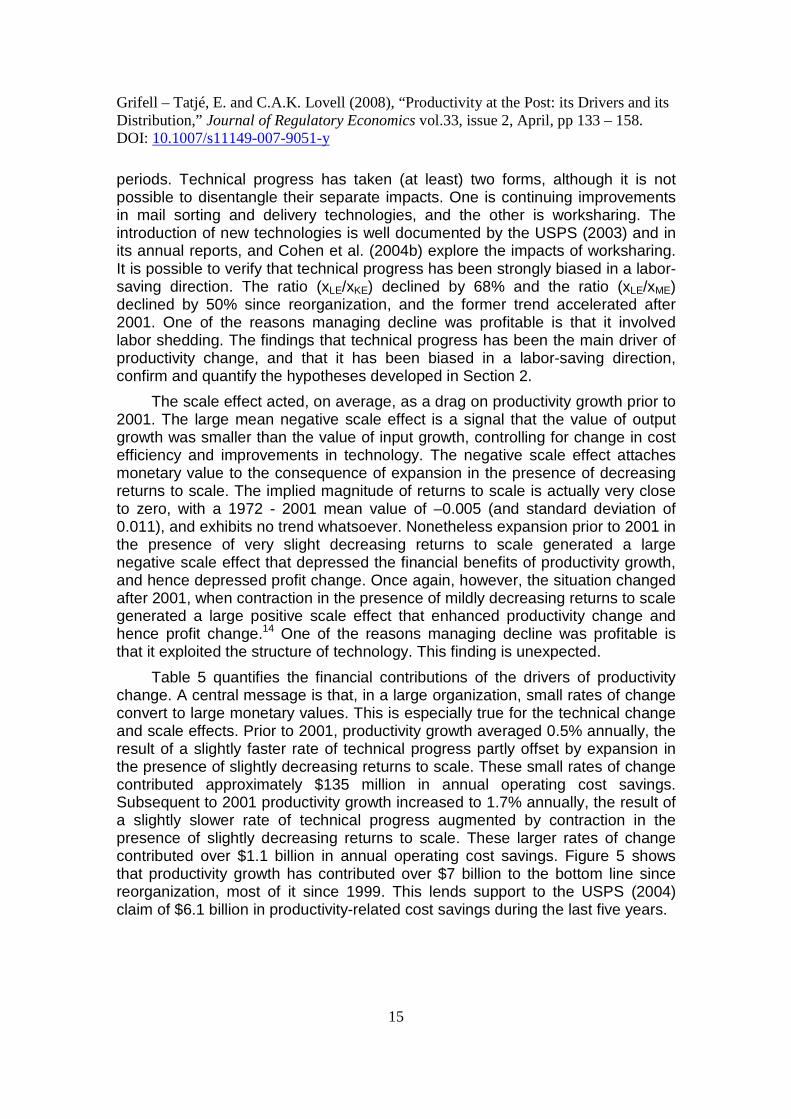
periods. Technical progress has taken (at least) two forms, although it is not possible to disentangle their separate impacts. One is continuing improvements in mail sorting and delivery technologies, and the other is worksharing. The introduction of new technologies is well documented by the USPS (2003) and in its annual reports, and Cohen et al. (2004b) explore the impacts of worksharing. It is possible to verify that technical progress has been strongly biased in a labor-saving direction. The ratio (xLE/xKE) declined by 68% and the ratio (xLE/xME) declined by 50% since reorganization, and the former trend accelerated after 2001. One of the reasons managing decline was profitable is that it involved labor shedding. The findings that technical progress has been the main driver of productivity change, and that it has been biased in a labor-saving direction, confirm and quantify the hypotheses developed in Section 2.

The scale effect acted, on average, as a drag on productivity growth prior to 2001. The large mean negative scale effect is a signal that the value of output growth was smaller than the value of input growth, controlling for change in cost efficiency and improvements in technology. The negative scale effect attaches monetary value to the consequence of expansion in the presence of decreasing returns to scale. The implied magnitude of returns to scale is actually very close to zero, with a 1972 - 2001 mean value of –0.005 (and standard deviation of 0.011), and exhibits no trend whatsoever. Nonetheless expansion prior to 2001 in the presence of very slight decreasing returns to scale generated a large negative scale effect that depressed the financial benefits of productivity growth, and hence depressed profit change. Once again, however, the situation changed after 2001, when contraction in the presence of mildly decreasing returns to scale generated a large positive scale effect that enhanced productivity change and hence profit change.14 One of the reasons managing decline was profitable is that it exploited the structure of technology. This finding is unexpected.

Table 5 quantifies the financial contributions of the drivers of productivity change. A central message is that, in a large organization, small rates of change convert to large monetary values. This is especially true for the technical change and scale effects. Prior to 2001, productivity growth averaged 0.5% annually, the result of a slightly faster rate of technical progress partly offset by expansion in the presence of slightly decreasing returns to scale. These small rates of change contributed approximately $135 million in annual operating cost savings. Subsequent to 2001 productivity growth increased to 1.7% annually, the result of a slightly slower rate of technical progress augmented by contraction in the presence of slightly decreasing returns to scale. These larger rates of change contributed over $1.1 billion in annual operating cost savings. Figure 5 shows that productivity growth has contributed over $7 billion to the bottom line since reorganization, most of it since 1999. This lends support to the USPS (2004) claim of $6.1 billion in productivity-related cost savings during the last five years.


16

6. Conclusions

The Postal Reorganization Act of 1970 sought to make the USPS a self-sustaining public corporation. The USPS has made impressive financial gains, but more than three decades after reorganization it remains in debt to the Federal Financing Bank. In this paper we have explored the sources and the beneficiaries of year-to-year change in operating profit at the USPS. We have exploited an internal database provided by the USPS to conduct our exploration. Identification of the sources and beneficiaries by variable requires only the conversion of these data to price and quantity indicators, but identification of the economic drivers of change in operating profit requires economic analysis.

At the initial stage of our exploration, we find poor price recovery performance to have exerted an increasingly heavy drag on financial performance, particularly in the two most recent sub-periods. The inability to compensate for the cost of input price increases with revenue-enhancing postal rate increases has reduced operating profit by nearly $100 million annually since reorganization, and by $365 million annually since 1992. This poor price recovery may reflect an inability of the USPS to contain costs by bargaining effectively with its input suppliers, particularly labor, whose price effect has dominated the input price effect throughout the period. This may also reflect an inability of the USPS to enhance revenue by persuading its regulator to grant postal rate increases adequate to cover increases in its inflated operating cost in a timely manner. In light of the weakness of the Postal Rate Commission, and the availability of the Federal Financing Bank, the first explanation seems more likely than the second.

The dual inability to contain cost and enhance revenue leads to an identification of the primary winners and losers from reorganization. Although price recovery was negative, output price increases were sufficient to generate a large positive output price effect throughout the period, making consumers of postal services consistently large losers. The magnitude of their losses exhibits no trend through the period, averaging a staggering $1.4 billion annually since reorganization. However even an output price effect of this magnitude was nearly offset by the labor price effect alone, making postal employees consistently large winners. The magnitude of labor’s gains also exhibits no trend through the period, and averages a slightly less staggering $1.3 billion annually. It is noteworthy that, despite all the changes involving USPS, its regulator, and its operating environment, this financial transfer has persisted for over three decades.

At the second stage of our exploration we apply economic analysis to the database in order to derive an independent measure of productivity change at the USPS and to identify its drivers. This requires decomposing a favorable quantity effect into a margin effect and a productivity effect. We find a small but improving margin effect, suggesting that rates determined by the PRC in the first two sub-periods were insufficient to cover ostensibly efficient unit operating cost, much less actual unit operating cost. However in the final two sub-periods rates


17

have been sufficient to cover ostensibly efficient unit operating cost and, in light of positive operating profit in most years since 1992, actual unit operating cost as well.

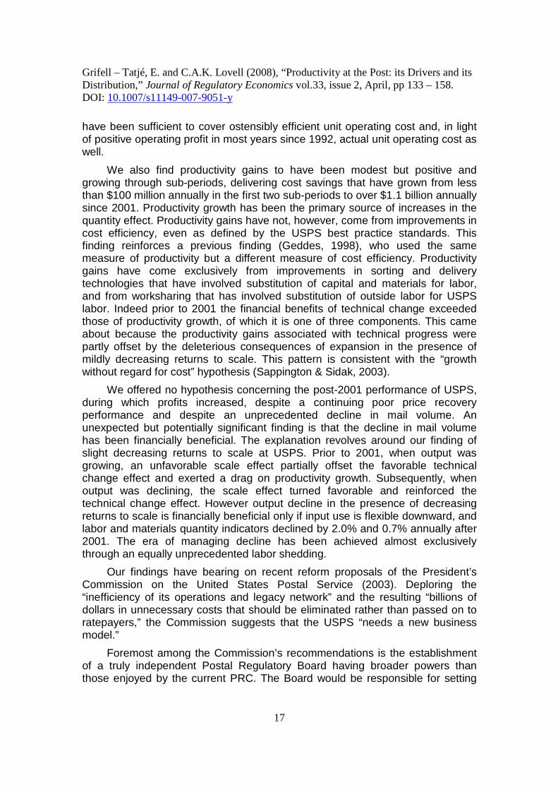
We also find productivity gains to have been modest but positive and growing through sub-periods, delivering cost savings that have grown from less than $100 million annually in the first two sub-periods to over $1.1 billion annually since 2001. Productivity growth has been the primary source of increases in the quantity effect. Productivity gains have not, however, come from improvements in cost efficiency, even as defined by the USPS best practice standards. This finding reinforces a previous finding (Geddes, 1998), who used the same measure of productivity but a different measure of cost efficiency. Productivity gains have come exclusively from improvements in sorting and delivery technologies that have involved substitution of capital and materials for labor, and from worksharing that has involved substitution of outside labor for USPS labor. Indeed prior to 2001 the financial benefits of technical change exceeded those of productivity growth, of which it is one of three components. This came about because the productivity gains associated with technical progress were partly offset by the deleterious consequences of expansion in the presence of mildly decreasing returns to scale. This pattern is consistent with the “growth without regard for cost” hypothesis (Sappington & Sidak, 2003).

We offered no hypothesis concerning the post-2001 performance of USPS, during which profits increased, despite a continuing poor price recovery performance and despite an unprecedented decline in mail volume. An unexpected but potentially significant finding is that the decline in mail volume has been financially beneficial. The explanation revolves around our finding of slight decreasing returns to scale at USPS. Prior to 2001, when output was growing, an unfavorable scale effect partially offset the favorable technical change effect and exerted a drag on productivity growth. Subsequently, when output was declining, the scale effect turned favorable and reinforced the technical change effect. However output decline in the presence of decreasing returns to scale is financially beneficial only if input use is flexible downward, and labor and materials quantity indicators declined by 2.0% and 0.7% annually after 2001. The era of managing decline has been achieved almost exclusively through an equally unprecedented labor shedding.

Our findings have bearing on recent reform proposals of the President’s Commission on the United States Postal Service (2003). Deploring the “inefficiency of its operations and legacy network” and the resulting “billions of dollars in unnecessary costs that should be eliminated rather than passed on to ratepayers,” the Commission suggests that the USPS “needs a new business model.”

Foremost among the Commission’s recommendations is the establishment of a truly independent Postal Regulatory Board having broader powers than those enjoyed by the current PRC. The Board would be responsible for setting


18

postal rate ceilings that rise by less than the rate of inflation, a sort of revenue cap regime. Rate ceilings would in turn motivate downward pressure on employee compensation. This recommendation is consistent with our identification of the price effect as the source of losses at USPS, and also with our identification of employees and consumers as the beneficiaries and victims of lax regulation since reorganization. The post-2001 era of managing decline is consistent with the Commission’s belief that the USPS can “grow smaller and stronger.” If these quantity effects can be sustained, then they would reinforce the price effects recommended by the Commission.


19

References

Bennet, T. L. (1920). The Theory of Measurement of Changes in Cost of Living. Journal of the Royal Statistical Society, 83, 455-62.

Cohen, R., Robinson, M., Scarfiglieri, G., Sheehy, R., Conandini, V.V., Waller, J,. & Xenakis, S., (2004a). The Role of Scale Economies in the Cost Behavior of Posts, available at http://www.prc.gov

Cohen, R., H., Robinson, M., Sheehy, R., Waller, J., & Xenakis, S., (2004b). Postal Regulation and Worksharing in the U.S., available at http://www.prc.gov

Davis, H. S. (1955), Productivity Accounting. Philadelphia: University of Pennsylvania Press.

Denny, M., Fuss, M., & Waverman, L., (1981). The Measurement and Interpretation of Total Factor Productivity in Regulated Industries, with an Application to Canadian Telecommunications. In T. G. Cowing & R. Stevenson, (Eds.), Productivity Measurement in Regulated Industries (pp. 179-218). New York: Academic Press.

Diewert, W. E. (2005). Index Number Theory Using Differences Rather than Ratios. American Journal of Economics and Sociology, 64(1), 347-95.

Fama, E. F., & Jensen, M. C. (1983). Agency Problems and Residual Claims. Journal of Law & Economics, 26(2), 327-49.

Geddes, R. (1998). The Economic Effects of Postal Reorganization. Journal of Regulatory Economics, 13, 139-56.

Geddes, R. (2003). Saving the Mail. Washington, DC: The AEI Press.

Geddes, R. R. (2005). Reform of the U.S. Postal Service. Journal of Economic Perspectives, 19(3), 217-32.

Grifell-Tatjé, E., & Lovell, C. A. K. (1999). Profits and Productivity. Management Science, 45(9), 1177-93.

Kendrick, J. W., & Creamer, D. (1961). Measuring Company Productivity: Handbook with Case Studies. Studies in Business Economics 74. New York: The Conference Board.

Lawrence, D., Diewert, W. E., & Fox, K. J. (2006). The Contributions of Productivity, Price Changes and Firm Size to Profitability. Journal of Productivity Analysis, 26(1), 1-13.

Miller, D. M. (1984). Profitability = Productivity + Price Recovery. Harvard Business Review, 62(3), 145-53.

President’s Commission on the United States Postal Service (2003). Embracing the Future: Making the Tough Choices to Preserve Universal Mail Service, available at http://www.treas.gov/offices/domestic-finance/usps/


20

Puiseux, L., & Bernard, P. (1965). Les Progrès de Productivité et Leur Utilisation a L’Électricité de France de 1952 a 1962. Études et Conjoncture, Janvier, 77-98.

Sappington, D. E. M., & Sidak, J. G. (2003). Incentives for Anticompetitive Behavior by Public Enterprises. Review of Industrial Organization, 22(3), 183-206.

US Department of Labor, Bureau of Labor Statistics (2007). Multifactor Productivity Trends, 2005, available at http://www.bls.gov/mfp

United States Postal Service (2003). The United States Postal Service: An American History, 1775-2002, available at http://www.usps.com/cpim/ftp/pubs/pub100.pdf

United States Postal Service (2004). 2004 United States Postal Service Annual Report, available at http://www.usps.com/history/anrpt04/


21

Figure 1. Total Factor Productivity Growth at the USPS

-3,000

-2,000

-1,000

0

1,000

2,000

3,000

4,000

196

3

196

6

1969

197

2

197

5

197

8

1981

1984

198

7

199

0

199

3

199

6

1999

200

2

Operating Profit, 1963-2004, $millions

Cumulative Total Factor Productivity, 1963-2004

0.950

1.000

1.050

1.100

1.150

1.200

1963

-62

1965

-64

1967

-66

1969

-68

1971

-70

1973

-72

1975

-74

1977

-76

1979

-78

1981

-80

1983

-82

1985

-84

1987

-86

1989

-88

1991

-90

1993

-92

1995

-94

1997

-96

1999

-98

2001

-00

2003

-02


22

Figure 2. Annual Operating Profit at the USPS

y

Tt+1 yt+1

Tt

yt

x xE xCE

t xt xCEt+1 xt+1

Figure 3. Decomposition of the Productivity Effect I


23

x2

Lt+1(yt+1)

Lt(yt) • xt+1

xCE

t+1

Lt+1(yt)

• xt

xCEt wt+1

wt xE

wt

x1

Figure 4. Decomposition of the Productivity Effect II


24

Cumulative Productivity Effect, 1972-2004, $million s

0

1,000

2,000

3,000

4,000

5,000

6,000

7,000

8,000

197

3-72

197

5-74

197

7-76

197

9-78

198

1-80

198

3-82

198

5-84

198

7-86

198

9-88

199

1-90

199

3-92

199

5-94

199

7-96

199

9-98

200

1-00

200

3-02

Figure 5. Cumulative Productivity Effect at the USP S


25

Table 1. Summary Statistics for United States Posta l Service, 1963 – 2004

1963 -

1972

1972 -

1982

1982 -

1992

1992 -

2001

2001 -

2004

1972 -

2004

Mean Operating Profit (current $ ) -1,308 -1,918 -799 638 1,176 -548

Growth Rate -7.8% 13.0% a a a a Mean Operating Revenues (current $) 5,473 13,506 32,959 56,434 67,410 36,684

Growth Rate 8.0% 9.6% 6.5% 3.5% 1.2% 7.2% Y Mean Workload (1972 $) 7,362 8,019 9,496 11,495 12,165 9,861

Growth Rate 2.0% 0.3% 2.2% 1.7% -0.3% 1.5% p Mean Output Price (1972 = 1.0) 0.737 1.679 3.430 4.892 5.542 3.477

Growth Rate 6.0% 9.3% 4.2% 1.8% 1.5% 5.8% Mean Cost (current $) 6,781 15,424 33,758 55,797 66,234 37,232

Growth Rate 8.0% 7.9% 6.3% 3.7% 0.2% 6.4% K Mean Capital Quantity (1972 $) 238 394 543 941 1,307 684

Growth Rate 7.2% 1.9% 5.1% 5.5% 1.7% 4.6%

wk Mean Capital Price (1972 = 1.0 ) 0.855 1.509 3.132 3.577 3.169 2.713

Growth Rate 3.0% 9.6% 2.0% -0.3% -3.9% 3.6% L Mean Labor Quantity (1972 $) 7,601 7,846 8,815 9,595 9,300 8,776

Growth Rate 1.9% -0.2% 1.5% 0.5% -2.0% 0.4%

wL Mean Labor Price (1972 = 1.0) 0.707 1.636 3.073 4.551 5.519 3.265

Growth Rate 6.9% 7.8% 4.8% 2.7% 2.4% 5.9% M Mean Materials Quantity (1972 $) 1,367 1,311 1,809 2,771 3,009 2,043

Growth Rate 0.5% 0.7% 3.9% 3.3% -0.7% 2.7%

wM Mean Materials Price (1972 = 1.0) 0.831 1.520 2.583 3.117 3.598 2.483

Growth Rate 3.2% 7.8% 1.8% 2.1% 1.1% 4.4% (a) Changes in sign


26

Table 2. Operating Profit Change Decomposition Mean Results by Period (millions of current dollar s)

Period Operating Profit Change = Bennet Price Indicator + Bennet Quantity Indicator

1972 - 1982 Mean 136.6 109.1 27.5

Std. Dev. 765.0 827.8 271.5

1982 - 1992 Mean 74.1 10.5 63.6

Std. Dev. 824.0 1,055.7 496.3

1992 - 2001 Mean -102.0 -398.4 296.4

Std. Dev. 1,067.8 1,797.7 997.8

2001 - 2004 Mean 879.7 -265.4 1,145.1

Std. Dev. 2,418.6 2,645.5 486.7

1972 - 2004 Mean 119.6 -99.5 219.2

Std. Dev. 1,053.4 1,361.8 685.2


27

Table 3. Bennet Quantity Indicator Primal Decomposi tion Mean Results by Period (millions of current dollars )

Period Bennet

Quantity Indicator

= Output Quantity - Capital Quantity - Labor Quantity - Material Quantity

1972 - 1982 Mean 27.5 38.6 8.3 -20.6 23.4

Std. Dev. 271.5

205.3

24.1

185.6

96.2

1982 - 1992 Mean 63.6 730.9 97.3 372.2 197.8

Std. Dev. 496.3

461.7

41.1

411.0

166.6

1992 - 2001 Mean 296.4 1,035.5 207.5 246.4 285.3

Std. Dev. 997.8

615.7

67.9

765.9

545.7

2001 - 2004 Mean 1,145.1 -252.7 96.6 -1,387.7 -106.8

Std. Dev. 486.7

1,103.1

126.4

747.7

45.0

1972 - 2004 Mean 219.2 508.0 100.4 49.1 139.3

Std. Dev. 685.2

688.7

94.6

702.0

324.4


28

Table 4. Bennet Quantity Indicator Dual Decomposit ion

Mean Results by Period (millions of current dollars )

Period Bennet

Quantity Indicator

= Profit Change - Output Price + Capital Price + Labor Price + Material Price

1972 - 1982 Mean 27.5 136.6 1,433.0 76.7 1,068.4 178.8

Std. Dev. 271.5

765.0 975.2

83.7

294.5

124.2

1982 - 1992 Mean 63.6 74.1 1,624.2 42.8 1,474.7 96.2

Std. Dev. 496.3

824.0 1,328.2

135.2

686.3

83.1

1992 - 2001 Mean 296.4 -102.0 1,144.0 -13.0 1,338.6 216.8

Std. Dev. 997.8

1,067.8 1,307.8

154.6

909.0

203.3

2001 - 2004 Mean 1,145.1 879.7 1,317.0 -219.9 1,649.9 152.5

Std. Dev. 486.6

2,418.6 1,579.3

196.7

1,112.9

95.8

1972 - 2004 Mean 219.2 119.6 1,400.6 13.1 1,325.9 161.2

Std. Dev. 685.2

1,053.4 1,194.5

151.8

702.7

141.8


29

Table 5. Bennet Quantity Indicator Economic Decompo sition Mean Results by Period (millions of current dollars )

Period Bennet

Quantity Indicator

Margin Effect + Productivity

Effect

Productivity Effect

=

Cost Efficiency

+ Technical

Change Effect + Scale Effect

1972 - 1982 Mean 27.5 -5.6 33.1 -39.6 101.1 -28.4

Std. Dev. 271.5 33.1 291.2 194.4 163.9 189.8

1982 - 1992 Mean 63.6 -26.2 89.8 47.6 324.2 -282.0

Std. Dev. 496.3 24.2 508.0 150.5 368.1 282.1

1992 - 2001 Mean 296.4 13.4 282.9 0.0 541.3 -258.3

Std. Dev. 997.8 22.5 1,008.3 0.0 684.4 656.8

2001 - 2004 Mean 1,145.1 10.6 1,134.6 0.0 680.1 454.5

Std. Dev. 486.7

16.4

480.6

0.0

681.8

202.1

1972 - 2004 Mean 219.2 -5.2 224.3 2.5 348.9 -127.0

Std. Dev. 685.2

30.0

689.7

137.0

489.3

442.9


30

∗ We thank the Financial Reporting and Analysis Division of the USPS for sharing its internal data. The views expressed in this paper are the authors' and not those of the United States Postal Service. We also thank Kengjai Watjanapukka for excellent research assistance, and “Segunda Convocatoria de Ayudas a la Investigación en Ciencias Sociales” of the Fundación BBVA for its generous financial support. Two referees provided very helpful comments on previous drafts, and Editor Michael Crew provided guidance. 1 Much of the available research on USPS and other postal networks is collected in a series of volumes edited by M. A. Crew and P. R. Kleindorfer and listed at http://crri.rutgers.edu/pub/ 2 This Section draws on USPS (2003) and Geddes (2003, 2005). 3 The USPS does report nonzero operating profit each fiscal year, and this value has to go somewhere. However we are reluctant to refer to the recipients of this operating profit or loss, whether they be the Federal Financing Bank or taxpayers, as “residual claimants,” in the traditional sense as expressed by Fama and Jensen (1983), because their claims are neither enforceable nor transferable (“alienable”). 4 A popular analytical framework for public sector service provision is one of budget constrained (or break-even constrained) revenue maximization. With frequent reference to USPS, Sappington and Sidak (2003) analyze the behavior of a “managerially-oriented public enterprise” that seeks to maximize a convex combination of revenue and profit. They show that such an organization is less concerned with controlling the cost incurred in expanding output(s) than a profit-seeking organization would be, and that such an organization has strong incentives to pursue anticompetitive activities. Although our focus is on productivity, financial performance and income distribution, and although they assign power to management rather than to labor, the predictions of their model are not inconsistent with some of the behavior of the USPS. 5 The analytical model has a single output, although it easily generalizes to multiple outputs, as in Grifell-Tatjé and Lovell (1999). We specify a single output because in its internal database the USPS reports a single output quantity index which, when divided into operating revenue, yields an implicit output price index. It also reports a mail quantity index and a delivery point index, and more detailed decompositions of both, but it is not possible to allocate operating revenue to mail quantity and delivery points, and so it is not possible to construct corresponding implicit price indexes. 6 Just as Fisher indexes are geometric means of Laspeyres and Paasche indexes, Bennet indicators are arithmetic means of Laspeyres and Paasche indicators. Diewert (2005) has demonstrated that Bennet quantity and price indicators satisfy a large number of tests analogous to those satisfied by Fisher quantity and price indexes. 7 The quantity effect can be expressed equivalently in growth rather than difference form, and decomposed as

p ytGy - Σ w nxntGxn quantity effect

= ( pyt - Σ w nxnCEt)Gy margin effect


31

+ (Σ w nxnCE

t)Gy – (Σ w nxnt)[Σ( w nxn

t/Σ w nxnt)Gxn] productivity effect

In the margin effect output growth Gy = [(yt+1/yt) – 1] is weighted by the difference between total revenue and cost-efficient total cost, using arithmetic mean output and input prices. In the productivity effect output growth is weighted by cost-efficient total cost, and input growth Σ( w nxn

t/Σ w nxnt)Gxn is weighted by actual total cost, with both

weights using arithmetic mean input prices. The weights convert a conventional productivity growth accounting formula Gy – Σ( w nxn

t/Σ w nxnt)Gxn expressed in

percentage terms to one expressed in value terms that shows the cost saving impact of productivity gains. 8 The productivity effect can be expressed equivalently in growth rather than difference terms, and decomposed as

(Σ w nxnCEt)Gy – (Σ w nxn

t)[Σ( w nxnt/Σ w nxn

t)Gxn] productivity effect

= Σ w nxnCEt[(xn

t – xnCEt)/xnCE

t] – Σ w nxnCEt+1[(xn

t+1 – xnCEt+1)/xnCE

t+1] cost efficiency effect

+ Σ w nxnE[(xnCEt - xnE)/xnE] technical change effect

+ Σ w nxnCEtGy - Σ w nxnE[Σ( w nxnE/Σ w nxnE)((xnCE

t+1 - xnE)/xnE)] scale effect

The scale effect is a productivity effect, measured net of cost efficiency change and technical change and using cost-efficient input cost shares w nxnE/Σ w nxnE. It is a pure scale effect evaluated on the surface of Tt+1, and signals increasing, constant or

decreasing returns to scale according as Gy ⋛ Σ( w nxnE/Σ w nxnE)Gxn. The weights convert a conventional scale economies formula expressed in percentage terms to one expressed in value terms that shows the cost saving impact of the exploitation of scale economies. 9 The productivity effect is interpreted broadly to include the impact of scale economies as well as the impacts of technical change and efficiency change. This broad interpretation corresponds to the US Bureau of Labor Statistics (2007) definition of multifactor productivity change as being “…designed to measure the joint influences on economic growth of technical change, efficiency improvements, returns to scale, reallocation of resources, and other factors.” Expressions (2) and (4) thus state that profit change is attributable to pricing power, a margin effect and productivity change. Apart from the margin effect, this is consistent with the interpretations of Miller (1984) and others in the accounting literature who attribute profit change to productivity change and price recovery change (their terminology for our price effect). Expression (5) converts a standard economic paradigm concerning the sources of productivity change, typically expressed in percentage terms, into a decomposition expressed in value terms. 10 Geddes (1998) examines 1930 – 1996 data in an effort to find structural breaks in various USPS indicators at reorganization. We examine 1972 – 2004 data in an effort to identify post-reorganization trends in a different set of USPS indicators. The research objectives are complementary, and the data are overlapping, and so it is possible, perhaps even likely, that some of the trends we uncover are continuations of discrete changes brought about by the PRA.


32

11 The USPS reports total operating expense in its Annual Reports. This figure differs from the total cost figure reported in the USPS internal database. For the last five years, the two figures are very close.

2004 2003 2002 2001 2000 USPS Annual Report 65851 63902 65234 65640 62992 USPS Internal Data 66929 65128 66503 66375 64294 % difference 1.6 1.9 1.9 1.1 2.1

In addition, because we do not include the general public service subsidy or the foregone revenue appropriation, our operating profit series is lower than what USPS reports as net income (loss) in its Annual Reports. 12 Tables 2 - 5 report post-reorganization sub-period means and standard deviations. Most standard deviations exceed their means by a wide margin, revealing year-to-year variability in the underlying data. For example, stamp prices change by discrete amounts, and at discrete and irregular intervals, which introduces variability into the output price, revenue and profit series. This in turn introduces variability into the decompositions reported in Tables 2 – 5. We emphasize that the source of year-to-year variability is the underlying data rather than our manipulations of the data. In addition, year-to-year variability causes sub-period results to be sensitive to the specification of terminal years. Annual variability needs to be kept in mind when interpreting the results of Tables 2 – 5, which are smoothed by averaging. Annual versions of Tables 2-5 are available on request. 13 It is worth noting, however, that the productivity effect itself is dwarfed by the input price effect obtained by adding the capital, labor and materials price effects in Table 4. The result has been continuously increasing unit costs that have exerted a drag on the bottom line. This finding is in accordance with the USPS “postal inflation index” (defined as C/y), which has increased 5.3% annually since reorganization. 14 Cohen et al. (2004a) suggest that the delivery function exhibits scale economies, and that other functions do not. We do not decompose USPS activities by function. Even though the delivery function accounts for approximately one third of total cost, our results suggest that aggregate cost-efficient operating cost has varied proportionately with aggregate output (which is a convex combination of a mail quantity index and a delivery point index). The two essential differences between the two approaches are that Cohen et al. define scale economies as the reciprocal of the elasticity of actual cost with respect to mail quantity, defined as the number of pieces of mail delivered, whereas we define scale economies as the reciprocal of the elasticity of cost-efficient cost with respect to what the USPS calls a workload index, defined as a convex combination of a mail quantity index and the number of delivery points. Historically growth in the mail quantity index has lagged that of the number of pieces of mail delivered, reflecting substitution away from high value mail categories into lower value mail categories. Our finding of slight decreasing returns to scale is consistent with this substitution, and supports the belief of the President’s Commission that the USPS can “grow smaller and stronger.”

repository productivity at the post

Documents