representation of linear operators by gabor multipliers · representation of linear operators...

Representation of linear operators

CREWES Research Report — Volume 15 (2003) 1

Representation of linear operators by Gabor multipliers

Peter C. Gibson, Michael P. Lamoureux, Gary F. Margrave

ABSTRACT

We consider a continuous version of Gabor multipliers: operators consisting of a short-time Fourier transform, followed by multiplication by a distribution on phase space (called the Gabor symbol), followed by an inverse short-time Fourier transform, allowing different localizing windows for the forward and inverse transforms. For a given pair of forward and inverse windows, which linear operators can be represented as a Gabor multiplier, and what is the relationship between the (non-classical) Kohn-Nirenberg symbol of such an operator and the corresponding Gabor symbol? These questions are answered completely for a special class of “compatible” window pairs. In addition, concrete examples are given of windows that, with respect to the representation of linear operators, are more general than standard Gaussian windows. The results in the paper help to justify techniques developed for seismic imaging that use Gabor multipliers to represent nonstationary filters and wavefield extrapolators.

INTRODUCTION This paper is concerned with the representation of linear operators by Gabor

multipliers. For us a Gabor multiplier is an operator of the form: a short-time Fourier transform, followed by multiplication by a distribution on phase space—called the Gabor symbol—followed by an inverse short-time Fourier transform. We explicitly allow the analysis window, upon which the forward short-time Fourier transform is based, to be different from the synthesis window, which serves as the basis for the inverse short-time Fourier transform.

More precisely, we study the representation of general (i.e., non-classical) Kohn-Nirenberg pseudodifferential operators—see for example [4]—by means of Gabor multipliers. As is well-known, the class of general Kohn-Nirenberg operators is simply all linear operators (essentially this is a version of the Schwartz kernel theorem—see (5) in Section 2.1). However, our aim is to analyze the correspondence between the Kohn-Nirenberg symbol, which in the general setting is an arbitrary distribution, and the Gabor symbol, of a given operator, provided the latter exists. The Gabor symbol of an operator depends on a choice of analysis and synthesis windows; indeed for a fixed window pair, there may be a limited class of linear operators that may be represented as a Gabor multiplier.

As far as we know the problem of representing Kohn-Nirenberg operators exactly by (our version of) Gabor multipliers is new, and in this paper we confine ourselves to the following two fundamental questions.

Gibson, Lamoureux, and Margrave

2 CREWES Research Report — Volume 15 (2003)

For a given pair of analysis and synthesis windows, which Kohn-Nirenberg operators may be represented as a Gabor multiplier?

Are there explicit formulas relating the Gabor and Kohn-Nirenberg symbols?

Much of the paper rests on a key technical notion of “compatible window pair”. For such windows we have a complete answer to both of the above questions. A common window choice for the short-time Fourier transform is a Gaussian, both as analysis and synthesis windows, and this serves as the prototype of a compatible window pair. One concrete result that emerges from our analysis of compatible windows is a new type of window, which we call an “extreme value” window—an analytic, rapidly decreasing window, with analytic, rapidly decreasing Fourier transform. It is more general than a Gaussian in the sense that the class of operators that can be represented as a Gabor multiplier based on Gaussian windows is a proper subset of the class that can be represented using extreme value windows.

The basic questions that we address here are motivated by a particular application, seismic imaging, where pseudodifferential operators play an important role [6,7] and Gabor multipliers have been successfully implemented as an efficient and flexible method of seismic deconvolution [8]. These implementations rest on the fact that there exist efficient numerical schemes, described in [5], by which to evaluate discretized versions of Gabor multipliers. But something that has been lacking so far is a theoretical analysis of the relationship between the original operators—i.e. extrapolators or filters—which are easily expressed as Kohn-Nirenberg operators, and the corresponding continuous Gabor multipliers that have been used to stand in for them. The results presented here serve to fill in the gap.

There is an important issue concerning the evaluation of linear operators in practical applications that we do not address in the present paper, namely, to quantify the degree of approximation to a continuous Gabor multiplier that is attained by discretized versions of it. For results in this direction, see, for example, Feichtinger and Nowak (2003) and [9].

The paper is organized as follows. The mathematical framework in which we formulate the problems described above is made precise in Section 2.1, where we fix the basic notational conventions. Theorem 1 of Section refsec-schwartzkernel gives a straightforward way to express the Schwartz kernel of a linear operator in terms of its Gabor symbol, which in turn yields an expression for the Kohn-Nirenberg symbol in terms of the Gabor symbol. The converse problem of expressing the Gabor symbol in terms of the Kohn-Nirenberg symbol seems to be much more difficult, and takes up the bulk of the paper. Section 2.3 provides the basic motivation for our key technical definition of compatible windows in Section 3.1. An alternate definition of compatibility, proved in Theorem 2 of Section 3.2 to be equivalent to the original, leads to a sequence of technical results in Section 3.2 that lay the groundwork for our main Theorems. These are Theorem 3 and Theorem 4 of Section 3.3. In Section 3.4 we apply Theorem 4 to show that extreme value windows serve to represent a wider class of linear operators as Gabor multipliers than is possible with Gaussian windows. We discuss briefly in Section 3.5 a natural extension of the notion of compatibility to singular windows. Lastly, Section 4 provides a short summary of the paper.



PRELIMINARIES

Notation and conventions Our notation is mostly standard, with the exceptions that: (i) we use the version of the

Fourier transform that has a factor of 2π in the exponent, and (ii) we take tempered distributions to be continuous, conjugate linear, rather than linear, functionals on the space of Schwartz class functions. Generally speaking, we deal with functions and distributions on nR , where the value of n is fixed within a given context, and nR is always the domain of integration, which we omit. We indicate a point in 2nR by a pair (x,y) of points , nx y∈R , and integration over 2nR is indicated by a pair of integral signs. For convenient reference, we have compiled in Table 1 a list of some of the function spaces and operators that we use repeatedly.

We work within the basic framework of Ln, the space of continuous, linear operators

': n nL →S S ,

making frequent use of the correspondence between Ln and '2nS [10]. More precisely,

given a linear operator L∈Ln, there is a unique distribution '2( ) nK K L= ∈S , its Schwartz

kernel, that satisfies the equation

, ,K Lθ ϕ ϕ θ⊗ = , nϕ θ∀ ∈S (1)

And conversely, given '2nK ∈S , the equation (1) evidently determines a unique nL∈L .

(Here ⊗ denotes the tensor product: ( , ) ( ) ( )f g x y f x g y⊗ = .) The adjoint of a linear operator nL∈L is the linear operator *

nL ∈L defined by the equation

* , ,L Lϕ θ θ ϕ= , nϕ θ∀ ∈S (2)

In order for the operator ψT , listed in Table 1, to be well-behaved, some restrictions have to be placed on ψ ; in this regard we introduce the notion of a “tempered change of variables”, as follows.

Definition 1. We say that a smooth, invertible map

: m mR Rψ → ,

is a tempered change of variables if each of the operators 1 1* *, , ,ψ ψ ψ ψ− −T T T T maps Sm into

Sm.

There is one tempered change of variables on R2n whose corresponding operator we assign a special notation:



_ψT_ = T , where _( , ) ( , )x y x y xψ = − . (3)

Given an arbitrary tempered distribution '2( , ) nxσ ξ ∈S , we write ( , )X Dσ for the

operator defined by the formula

2

( ) ( ) ( ) ( ) ( )n nix

X D X D x x de π ξσ σ ϕ σ ξ ϕ ξ ξ′ ⋅

, : → ; , = , .∫S S F (4)

(Here : n nX →R R denotes the identity map, so that, for example, ( )X x xα α= . D

stands for the differential operator 12

Diπ

= ∂ .) We refer to ( , )X Dσ as a Kohn-

Nirenberg pseudodifferential operator; the distribution ( , )xσ ξ is its Kohn-Nirenberg symbol.

In the context of classical pseudodifferential operators, where the symbol ( , )xσ ξ is required to be smooth and of bounded growth, the integral on the right-hand side of (4) is inherently well-defined. A simple way to give the integral an unambiguous interpretation in the present much more general setting is to define ( , )X Dσ in terms of its Schwartz kernel:

2( ( , ))K X Dσ σ= T_F . (5)

Since each of the operators T_ and F2 carries '2nS bijectively onto itself, it is evident

from the representation (5) that the class of Kohn-Nirenberg pseudodifferential operators on Rn is identical with nL itself. Among the various ways to represent a linear operator, however, the Kohn-Nirenberg symbol and accompanying formal representation (4) are of particular interest since, from the physical point of view, they are natural both for partial differential operators and for nonstationary filters [4]. In other words, in applications one is sometimes given the Kohn-Nirenberg symbol of a linear operator directly.

Note that the Kohn-Nirenberg symbol Lσ and the Schwartz kernel K(L) of a linear operator ': n nL →S S both belong to '

2nS . But there is a sense in which these are distinct

versions of '2nS , in that Lσ is a distribution on phase space, n n×R R , while K(L) is a

distribution on the cross product n n×R R of the underlying space with itself. Indeed, since it is sometimes useful to make this distinction between space and frequency, we reserve ξ and η for frequency variables, using other letters (such as x,y,τ,t,v,w) for spacial variables.



Table 1. Notation

Function and distribution spaces Sn Schwartz class functions : n nϕ →R R

'nS (conjugate linear) tempered distributions : nu →CS

Pn ∞C functions : n nϕ →R R such that αϕ∂ is bounded by a

polynomial Pα for every multi-index α

Operators Description Symbol Action on functions Adjoint

Composition with a change of variables

: m mψ →R R

ψT ϕ ϕ ψ *1 1det Jψ ψ ψ− −=T T

Fourier transform

( )' '

: n n

n n

→

→

S SFS S

2

( ) ( )

( )i x

x

e x dxπ ξ

ϕ ϕ ξ

ϕ− ⋅= ∫

1∗ −=F F

Partial Fourier transform

( )2 2

' '2 2

: n n

n n

→

→1S SFS S

1

2

( ) ( )

( )i x

x y y

e x y dxπ ξ

ϕ ϕ ξ

ϕ− ⋅

, ,

= ,∫F

1

1 1∗ −=F F

Partial Fourier transform

( )2 2

' '2 2

: n n

n n

→

→2S SFS S

1

2

( ) ( )

( )i y

x y x

e x y dyπ η

ϕ ϕ η

ϕ− ⋅

, ,

= ,∫F

1

2 2∗ −=F F

Modulation

( )' '

: n n

n n

ξ→

→

S SMS S

2( ) ( )i xx e xπ ξϕ ϕ⋅ ξ ξ

∗−=M M

Translation

( )' '

: n n

n n

→

→xS STS S

( ) ( )t t xϕ ϕ −

x x∗

−=T T

Multiplication by 'ma∈ S : mNα → '

mP S

aϕ ϕ —



The Schwartz kernel of a general Gabor multiplier

If ng : →R C is measurable and bounded by a polynomial, then the formula

( )g xV x M T gξϕ ξ ϕ, = ,

defines a short-time Fourier transform 2g n nV : →S P with analysis window g. The basic theory of short-time Fourier transforms is described in [4]. For nγ ∈S , the range of Vγ

lies in 2nS ; the adjoint Vγ∗ of Vγ is the map

2n nV V u u Vγ γ γϕ ϕ∗ ′ ′ ∗: → ; , = ,S S .

If the distribution 2nu ′∈S happens to be an 2L function, then V uγ∗ is given by the formula

( ) ( ) ( )xV u t u x M T t dxdγ ξξ γ ξ∗ = , .∫∫

Definition 2. Let ng : →R C be measurable and bounded by a polynomial, and let

nγ ∈S . If in addition 0g γ, ≠ , then we say that each of ( )g γ, and ( )gγ , is a window

pair on nR .

It is a basic fact about the short-time Fourier transform that for any window pair ( )g γ, , the map

1g n nV V

g γγ∗ : →

,S S (6)

is the identity. Recall from Table 1 that we use the symbol aN to denote multiplication by a.

Definition 3. Given a window pair ( )g γ, on nR and a distribution 2na ′∈S , we call

1ga a gV N V

gγ

γγ, ∗=

,M

a Gabor multiplier; we refer to the distribution a as its Gabor symbol.

(Note that Feichtinger and Nowak [1] use the term “short-time Fourier transform multiplier” for a Gabor multiplier based on identical windows ( )g g, , while in Feichtinger and Nowak (2003) “Gabor multiplier” refers to a more general object than we have defined.) A Gabor multiplier, in the sense of Definition 3, is a linear operator belonging to nL . Its adjoint is also a Gabor multiplier, and the precise connection between the two works out as follows.



Proposition 4. For any window pair ( )g γ, and any distribution 2na∈S , the adjoint of

the Gabor multiplier gaγ,M is g g

a aγ γ∗, ,

=M M .

Roughly speaking, the defining structure of a Gabor multiplier means that it carries an implicit diagonalization on phase space. From the theoretical point of view, this fact makes it desirable to express, if possible, a given linear operator nL∈L as a Gabor multiplier, the structure of the operator then being encoded in its Gabor symbol. It is also desirable to express an operator as a Gabor multiplier from the point of view of applications, since there exist fast computational methods to evaluate discretized Gabor multipliers [5].

The main problem that we are concerned with in the present paper is to express a given Kohn-Nirenberg pseudodifferential operator as a Gabor multiplier. Before considering the issue in detail, we deal briefly with the converse problem, of expressing a given Gabor multiplier as a pseudodifferential operator. In light of the expression (5) for the Schwartz kernel of a pseudodifferential operator, the latter problem is equivalent to computing the Schwartz kernel of a Gabor multiplier. This turns out to be relatively straightforward, and can be carried out in full generality. In stating the basic result we make use of the following notation. Let 4 2n nS : →S S denote the map defined by

( ) ( )S x x xρ ξ ρ ξ ξ, = , , ,− .

The corresponding adjoint is the map

2 4n nS S u u Sϕ ϕ∗ ′ ′ ∗: → ; , = , .S S

Theorem 1. An arbitrary Gabor multiplier gaγ,M has Schwartz kernel

1( )ga gV S a

gγ

γγ, ∗ ∗

⊗= .,

K M (7)

Proof. Note that

1ga ga V V

gγ

γϕ θ ϕ θγ

, , = ,,

M

and

2 2( ) ( ) ( ) ( ) ( )it igV V x t e g t x dt e x dπ ξ π τ ξ

γϕ θ ξ ϕ θ τ γ τ τ− ⋅ − ⋅, = − −∫ ∫

2 2( ) ( ) ( ) ( )it it e g t x e x d dtπ ξ π τ ξϕ θ τ γ τ τ⋅ − ⋅= − −∫∫



2 ( ) ( ) ( ) ( )i te x g t x t d dtπ τ ξγ τ θ ϕ τ τ− ⋅= − − ⊗ ,∫∫ (8)

2 ( ) ( )( ) ( ) ( )i tx xe T g t t d dtπ τ ξ ξ γ τ θ ϕ τ τ− , ⋅ ,−,= ⊗ , ⊗ ,∫∫

( )gV x xγ θ ϕ ξ ξ⊗= ⊗ , , ,− .

Thus,

1

1

ga g

g

a SVg

V S ag

γγ

γ

ϕ θ θ ϕγ

θ ϕγ

,⊗

∗ ∗⊗

, = , ⊗,

= , ⊗ .,

M

Since generalized Kohn-Nirenberg operators encompass all of nL , given an arbitrary Gabor multiplier g

aγ,M on nR , there exists a distribution 2nσ ∈S such that

( ) gaX D γσ ,, =M . By Theorem 1, this is equivalent, in terms of Schwartz kernels, to the

equation

21

gV S ag γσγ

∗ ∗⊗= ,

,T_F (9)

which can be solved for σ in terms of a to yield

1 12

1gV S a

g γσγ

− − ∗ ∗− ⊗= .

,F T (10)

In contrast, there is no obvious way to solve equation (9) for a in terms of σ , since neither of the operators gVγ

∗⊗ or S ∗ is injective. Indeed, determining the Gabor symbol

that corresponds to a given Kohn-Nirenberg symbol seems to be a much more intricate problem.

Identical Gaussian windows Let us specialize to the case of a window pair consisting of identical Gaussians,

2

( ) ( ) tg t t e πγ −= = , where we use the notation 2t t t= ⋅ for nt∈R . The special structure of these windows means that we can obtain an alternate formula for the Schwartz kernel of any Gabor multiplier based on them.

The key point in our proof of Theorem 1, at which we can take advantage of our present choice of Gaussian windows, is the integral (8). The integrand involves the product



2 2

2 22 2

( ) ( )

2 ( ) ( )

( ) ( )t

x t x

x t

x g t x e ee eτ π

π τ π

π τ

γ τ+

− − − −

− − − −

− − =

= .

Thus, in terms of the tempered change of variables

2( ) ( )tv w tτ τ+, = , − ,

we see that ( ) ( )x g t xγ τ − − has the form

1 2( ) ( ) ( ) ( )x g t x G v x G wγ τ − − = − , (11)

where 22

1( ) vG v e π−= and 2

22 ( ) wG w e

π−= . Substituting (11) into the expression (8) for

gV Vγϕ θ , we obtain

2 ( )1 2( ) ( ) ( )i t

gV V e G v x G w t d dtπ τ ξγϕ θ θ ϕ τ τ− ⋅= − ⊗ ,∫∫

12 1

1 2( ) ( ) ( ) detiwe G v x G w v w J dvdwπ ξψ

θ ϕ ψ −⋅ −= − ⊗ , | |∫∫

2( 0) 1 2 ( ) ( )iwxe T G G v w v w dvdwπ ξ

ψθ ϕ⋅ ∗,= ⊗ , ⊗ ,∫∫ T

2( 0) 1 2 ( ) ( )iwxe T G G v w v w dv dwπ ξ

ψθ ϕ⋅ ∗,

= ⊗ , ⊗ ,

∫ ∫ T

( )12 2 11 GG ψθ ϕ− ∗= ⊗ ∗ ⊗F T , (12)

where 11( ) ( )v G vG = − and 1∗ denotes convolution with respect to the first n variables. Replacing 1

2−F with 1

2−F , and carrying 1F through the convolution, we obtain from (12)

that

( )12 11gV V GGγ ψϕ θ θ ϕ− ∗= ⊗ ⊗F FT .

Proceeding as in the proof of Theorem 1, this leads to the following formula for the Schwartz kernel of g

aγ,M :

21

11

1( )ga GG

K N ag

γψγ

, −⊗=

,M T F F . (13)

Recalling that 2

( ) ( ) tg t t e πγ −= = , 22

1( ) vG v e π−= , and 2

22 ( ) wG w e

π−= , we have

2 2

2 2 221( ) 2

n ww e eGGπ πηη − − −⊗ , = .

Since 22 22t ng e dtπγ − /, = =∫ , the formula (13) simplifies as in the next proposition.



Proposition 5. Let 2

( ) ( ) tg t t e πγ −= = be identical Gaussians on nR . Then for any

2na ′∈S , the Schwartz kernel of gaγ,M is

11( )g

a GK N aγψ

, −= ,M T F F (14)

where 2nG : →R R is the Gaussian 2

2 ( )( ) wG w eπ ηη − ,, = and ψ is the tempered change of

variables 2( ) ( )tt tτψ τ τ+, = , − .

Each of the operators 11 GNψ−, ,T F and F occurring in the expression (14) for the

Schwartz kernel of gaγ,M is injective. Therefore if ( )g

a X Dγ σ, = ,M , we can, by comparing the Schwartz kernels of the two operators, express the Gabor symbol of g

aγ,M in terms of

σ as

2

2 ( )1 where ( ) y i yHa N H y e

π η π ησ η , − ⋅−= , , = .F F (15)

Moreover, for a given 2nσ ′∈S , the operator ( )X Dσ , can be expressed as a Gabor multiplier based on identical Gaussian windows only if the expression (15) yields a well-defined tempered distribution a . (Note that (15) cannot be written as a convolution, because the rapidly increasing function H does not have a Fourier transform.)

Are there window pairs ( )g γ, other than identical Gaussians for which one can obtain results analogous to these? The purpose of this paper is to describe a class of window pairs for which this is possible.

MAIN RESULTS

Definition and examples of compatible window pairs The expression (14) for the Schwartz kernel of a Gabor multiplier based on identical

Gaussians is the basis for the formula (15). With an eye to obtaining more general results along these lines, we investigate the class of all window pairs for which a formula analogous to (14) exists. In this regard the essential property of a Gaussian is the factorization rule (11), so we focus on the class of all window pairs that obey such a rule. This leads directly to the following key technical notion.

Definition 6. We say that a window pair ( )g γ, on nR is compatible, and that g and γ are compatible windows, if there exist functions 1 2

nG G, : →R C and a tempered change of variables ( ) ( )v w tψ τ, = , with w t tau= − such that for every nt xτ , , ∈R ,

1 2( ) ( ) ( ) ( )x g t x G v x G wγ τ − − = − .



Note that our derivation of formula (13) in Section 2.2 is valid for arbitrary compatible windows as we have just defined them. Hence we immediately have the following result.

Proposition 7. Let ( )g γ, be a compatible window pair on nR . Then for any 2na ′∈S , the Schwartz kernel of g

aγ,M is

21

11

1( )ga GG

K N ag

γψγ

, −⊗= ,

,M T F F

where 1 2G G, and ψ are related to ( )g γ, as in Definition 6.

If ( )g γ, is compatible then so is ( )gγ , . The precise connection between the accompanying sets of functions as stated below may be easily verified. Here we write

2 2n nψ↔ : →R R for the change of variables ( ) ( )x y y xψ↔ , = , , and we use the notation

( ) ( )F x F x= − .

Proposition 8. Let ( )g γ, be a compatible window pair on nR , so that

1 2( ) ( ) ( ) ( )x g t x G v x G wγ τ − − = − ,

in accordance with Definition 6. Then the reverse window pair ( )gγ , is also compatible and satisfies the equation

1 2( ) ( ) ( ) ( )g x t x G v x G wτ γ ′ ′ ′ ′− − = − ,

where 1 21 2G GG G′ ′= , = , and ( ) ( )v w v wψ′ ′

↔, = , .

Table 2 lists several families of compatible window pairs, alongside their corresponding factorizations and changes of variables, as prescribed by Definition 6. The class of compatible window pairs is easily seen to be invariant with respect to a number of elementary operations: rescaling, translation and modulation of either window, and linear change of variables applied simultaneously to both windows. This observation shows that the list in Table 2 is not complete. On the other hand, the window pairs listed in Table 2 are reasonably representative. For example, it turns out that every non-negative compatible window pair on 1R can be obtained by translating, dilating, reversing or rescaling the given examples, or by reversing the order of a window pair obtained this way. This is a rather involved technical result that will be presented in a forthcoming paper [3].



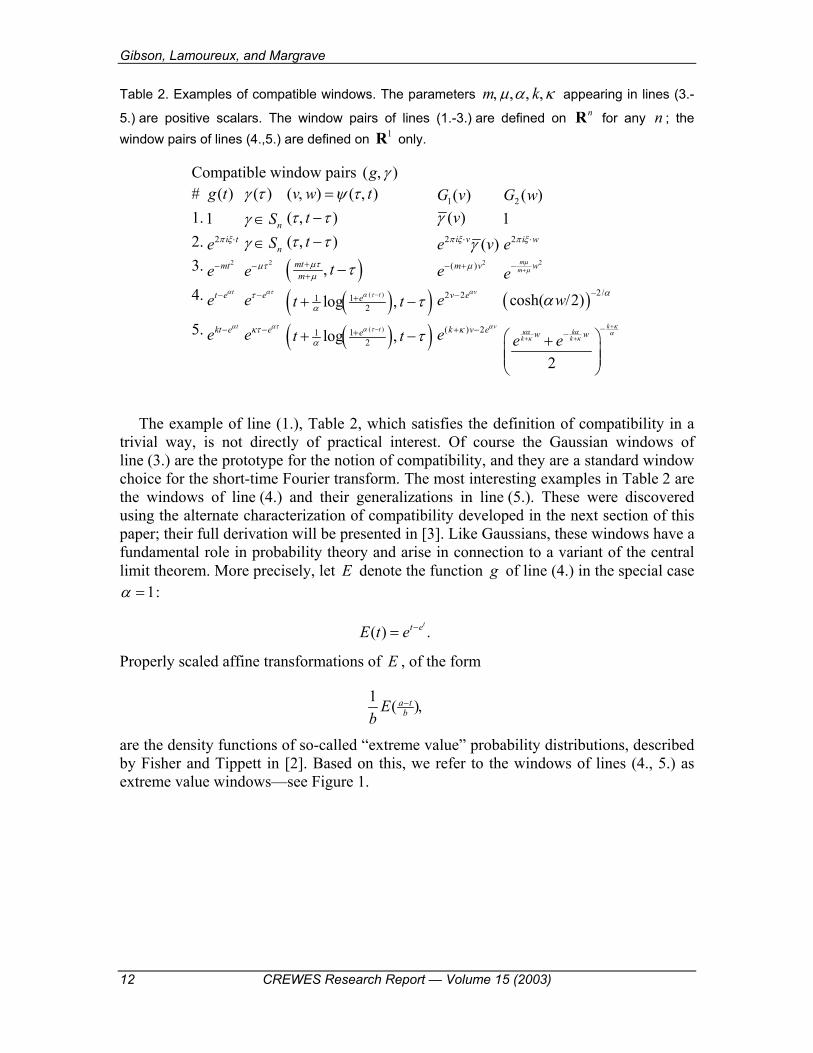
Table 2. Examples of compatible windows. The parameters m kµ α κ, , , , appearing in lines (3.-

5.) are positive scalars. The window pairs of lines (1.-3.) are defined on nR for any n ; the window pairs of lines (4.,5.) are defined on 1R only.

Compatible window pairs ( )g γ, # ( )g t ( )γ τ ( ) ( )v w tψ τ, = , 1( )G v 2 ( )G w 1. 1 nSγ ∈ ( )tτ τ, − ( )vγ 1 2. 2 i te π ξ ⋅

nSγ ∈ ( )tτ τ, − 2 ( )i ve vπ ξ γ⋅ 2 i we π ξ ⋅ 3. 2mte−

2

e µτ− ( )mtm tµτ

µ τ++ , − 2( )m ve µ− +

2mm weµµ+−

4. tt eeα− ee

αττ − ( )( )( )112log tet tα τ

α τ−++ , − 2 2 vv eeα− ( ) 2cosh( 2)w αα − //

5. tkt eeα− ee

ατκτ − ( )( )( )112log tet tα τ

α τ−++ , − ( ) 2 vk v eeακ+ −

2

kk

k kw we eκ

κα α ακ κ

+

+ +−− +

The example of line (1.), Table 2, which satisfies the definition of compatibility in a trivial way, is not directly of practical interest. Of course the Gaussian windows of line (3.) are the prototype for the notion of compatibility, and they are a standard window choice for the short-time Fourier transform. The most interesting examples in Table 2 are the windows of line (4.) and their generalizations in line (5.). These were discovered using the alternate characterization of compatibility developed in the next section of this paper; their full derivation will be presented in [3]. Like Gaussians, these windows have a fundamental role in probability theory and arise in connection to a variant of the central limit theorem. More precisely, let E denote the function g of line (4.) in the special case

1α = :

( )tt eE t e −= .

Properly scaled affine transformations of E , of the form

1 ( )a tbE

b− ,

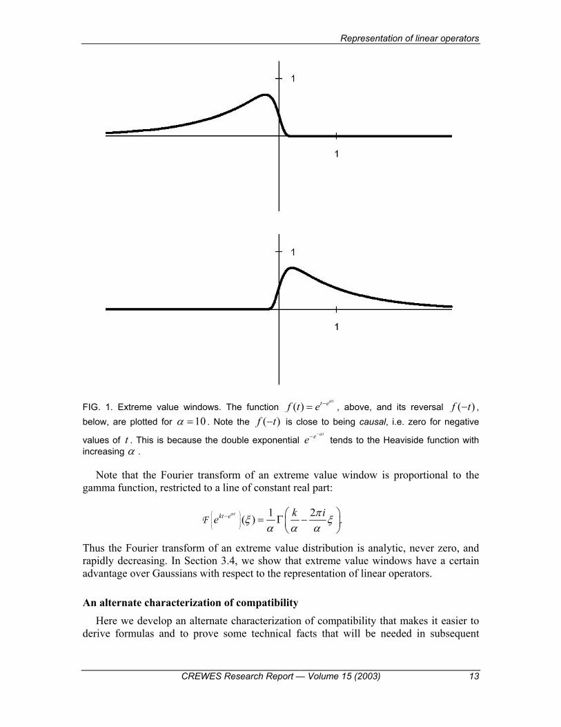
are the density functions of so-called “extreme value” probability distributions, described by Fisher and Tippett in [2]. Based on this, we refer to the windows of lines (4., 5.) as extreme value windows—see Figure 1.



FIG. 1. Extreme value windows. The function ( )tt ef t e

α−= , above, and its reversal ( )f t− , below, are plotted for 10α = . Note the ( )f t− is close to being causal, i.e. zero for negative

values of t . This is because the double exponential tee

α−− tends to the Heaviside function with increasing α .

Note that the Fourier transform of an extreme value window is proportional to the gamma function, restricted to a line of constant real part:

1 2( )tkt e k ie

α πξ ξα α α

− = Γ − .

F

Thus the Fourier transform of an extreme value distribution is analytic, never zero, and rapidly decreasing. In Section 3.4, we show that extreme value windows have a certain advantage over Gaussians with respect to the representation of linear operators.

An alternate characterization of compatibility Here we develop an alternate characterization of compatibility that makes it easier to

derive formulas and to prove some technical facts that will be needed in subsequent



sections. The arguments given here are purely technical; they build toward our main results which are presented in the following Section 3.3.

Let ( )g γ, be a compatible pair on nR with corresponding functions 1 2G G, and tempered change of variables ( ) ( )v w tψ τ, = , , as stipulated in Definition 6. It can be deduced from the basic equation,

1 2( ) ( ) ( ) ( ) nx g t x G v x G w t xγ τ τ− − = − ∀ , , ∈ ,R (16)

that there are several simplifying assumptions to be made concerning 1 2G G, and ψ without any incumbent loss of generality.

Firstly, note that 1 2( ( ) ) ( ) ( ) ( )G v t x G t x g t xτ τ γ τ, − − = − −

(( ) ( )) (0 ( ))t x t g x tγ τ= − − − − −

1 2( ( 0) ( )) ( )G v t x t G tτ τ= − , − − −

1 2( ( 0) ) ( )G v t t x G wτ= − , + − . (17)

This leads to the first of our simplifying propositions.

Proposition 9. It may be assumed without loss of generality that

( ) ( 0) nv t v t t tτ τ τ, = − , + ∀ , ∈ .R (18)

Proof. Suppose that (18) fails to hold, and consider the new function v′ , defined by

( ) ( 0) nv t v t t tτ τ τ′ , = − , + ∀ , ∈ .R

Based on the fact that ( )v wψ = , is a tempered change of variables, it may be verified that the change of variables ( )v wψ ′ ′= , is tempered also. And by construction,

( ) ( 0) nv t v t t tτ τ τ′ ′, = − , + ∀ , ∈ .R

Now, applying the identity (17) yields

1 2 1 2

1 2

( ) ( ) ( ( 0) ) ( )

( ) ( )

G v x G w G v t t x G w

G v x G w

τ′

− = − , + −

= − .

Therefore the defining equation (16) remains satisfied if we replace ψ by the new change of variables ψ ′ .



Proposition 10. It may be assumed without loss of generality that (0 0) 0v , = .

Proof. The equation that defines compatibility, (16), remains satisfied if 1G is replaced by

1 1( ) ( (0 0))G y G y v′ = + ,

and v is replaced by

( ) ( ) (0 0)v t v t vτ τ′ , = , − , .

The modified change of variables ( )v wψ ′ ′= , is tempered, and by construction (0 0) 0v′ , = ..

Proposition 11. Without loss of generality, 2 (0) 1G = and 1G gγ=

Proof. Substituting 0w = (i.e., t τ= ) and 0x = into the equation (16) yields

1 2( ) ( ) ( ( )) (0)t g t G v t t Gγ = , . (19)

Since 0 g gγ γ≠ , = ∫ , it follows from (19) that that 2 (0) 0G ≠ . The equation (16) evidently remains satisfied if 2G is replaced by

2

12(0)G G and 1G is replaced by 2 1(0)G G ,

so we may assume 2 (0) 1G = .

Assuming in addition that (18) holds and that (0 0) 0v , = , we have that ( ) (0 0)v t t v t t, = , + = . It then follows from equation (19) that 1( ) ( ) ( )G t t g tγ= .

It will streamline subsequent arguments to assume that 1 2G G, and ψ have the forms given in Propositions 9, 10, and 11. We now introduce the notion of “product-translation commutativity” for a window pair.

Definition 12. Let ( )g γ, be a window pair on nR . We say that ( )g γ, is product-translation commutative, or that g and γ are product-translation commutative, if there exist functions nC : →R C and n nζ : →R R such that for every nw∈R ,

( )( ) ( )w wgT C w T gζγ γ= , (20)

and such that ( ) ( ( ) )t t t tτ ζ τ τ, − − , − is a tempered change of variables.

Although it is not immediately obvious, product-translation commutativity of a window pair is equivalent to compatibility. This fact facilitates the analysis of compatibility.



Theorem 2. A window pair ( )g γ, is product-translation commutative if and only if it is compatible. Moreover, if a window pair ( )g γ, has this property then, without loss of generality, the terms occurring in the respective defining equations,

( ) 1 2( ) ( ) and ( ) ( ) ( ) ( )w wgT C w T g x g t x G v x G wζγ γ γ τ= − − = − ,

may be assumed to be related by the formulas

2 ( ) ( ) and ( ) ( 0)G C v t t t y v yτ ζ τ ζ= , , = − − = − − , .

Proof. We prove the equivalence of Definitions 6 and 12; the stated formulas emerge in the course of the proof.

Suppose that ( )g γ, is compatible, with associated functions 1 2G G, and ψ that satisfy the properties in Propositions 9, 10, and 11. The basic equation of Definition 6, equation (16), can be written symbolically as

( ) ( 0) 1 2x x xT g T G Gψγ, ,⊗ = ⊗T

( ) ( 0) 1 2x x xg T T G Gψγ − ,− ,⇔ ⊗ = ⊗T

1 2( ) ( ( ) ) ( )g t G v x t x x G wγ τ τ⇔ ⊗ , = + , + − . (21)

Define ( ) ( 0)y v yζ = − − , , so that substituting x t= − into (21) yields

( )g tγ τ⊗ , = 1 2( ( 0) ) ( )G v t t G wτ − , +

= 1 2( ( )) ( )G t w G wζ−

= 2( ( )) ( ( )) ( )g t w t w G wζ γ ζ− − (by Proposition 11) (22)

The identity w t τ= − implies that ( ) ( )wg t gT tγ τ γ⊗ , = . Therefore (22) is equivalent to the equation

2 ( )( ) ( ) ( )( )w wgT t G w T g tζγ γ= . (23)

Note that ( ) ( 0) ( )v t v t t t tτ τ ζ τ, = − , + = − − , so the tempered change of variables ( )v wψ = , is precisely the map ( ) ( ( ) )t t t tτ ζ τ τ, − − , − . Together with (23), this

verifies that the pair ( )g γ, conforms to Definition 12 of product-translation commutativity, with 2C G= .

Conversely, suppose that the window pair ( )g γ, is product-translation commutative, with associated functions C ζ, as in Definition 12. Set ( ) ( )v t t tτ ζ τ, = − − , so that



( ( ) ( )) ( ( ) )v t w t t t tτ τ ζ τ τ, , , = − − , − is a tempered change of variables. As before, ( ) ( )wg t gT tγ τ γ⊗ , = , so by definition,

( )

( ) ( ( )) ( ( )) ( )( ) ( ( ) ) ( ( ) ) ( )

( )( ) ( )x x

g t t w g t w C wT g t t w x g t w x C w

g v x C w

γ τ γ ζ ζγ τ γ ζ ζ

γ,

⊗ , = − −⇒ ⊗ , = − − − −

= − .

Thus ( )g γ, conforms to Definition 6, with associated functions 1G gγ= , 2G C= and ( )v wψ = , .

We are now in a position to derive two additional formulas concerning compatible window pairs. Recall that n nX : →R R denotes the identity map; kX denotes its k -th

component. We write ( )gX γ∗ for the vector ( )1( ) ( )ngX … gXγ γ∗ , , ∗ , and similarly

( )1 ngX gX … gXγ γ γ, = , , , , . A tilde over a function indicates reflection in the

argument: ( ) ( )F y F y= − .

Proposition 13. If ( )g γ, is a compatible pair then, without loss of generality, the associated function 2G is given by the formula

2gGgγγ∗

= .,

(24)

And the change of variables ψ can be expressed as ( ) ( ( ) )t t t tψ τ ζ τ τ, = − − , − , where the restriction of ζ to points w at which 2 ( ) 0G w ≠ is given by the formula

( ) gXgXgg

γγζγγ,∗

= − .,∗

(25)

Proof. By Theorem 2, g and γ satisfy the equation

2 ( )( ) ( )w wgT G w T gζγ γ= .

Integrating both sides over nR and rearranging terms yields



2

( )

( )( )

( )

( )

w

w

gTG wT g

g w

g

g wg

ζ

γ

γ

γ

γ

γγ

=

∗=

∗=

,

∫∫

∫.

Observe that

2 ( )

2

( ) ( )

( ) ( )

( ) ( ( ))

w

w

gX w XgT

XG w T g

G w X w g

ζ

γ γ

γ

ζ γ

∗ =

=

= + .

∫∫

∫

Also,

2 ( )g G w gγ γ∗ = , ,

so, provided 2 ( ) 0G w ≠ , the right-hand side of (25) becomes

2

2

( ) ( ( )) ( ) ( )( )

gX g gXG w X w g w ac gX g wG w g g g g

γ γ γζ γ ζ γ γ ζγ γ γ γ

, , ,+− = + − , , = .

, , , ,∫

It turns out that 2G can never be zero, so that in fact the formula (25) is valid everywhere, but we will not prove this in the present paper (see [3]).

Next we prove some technical results, in anticipation of the coming section, where we relate the Gabor symbols of Gabor multipliers based on compatible windows to their Kohn-Nirenberg symbols.

Proposition 14. Let ( )g γ, be a compatible window pair, with associated functions

1 2G G, . Then without loss of generality

2 21

1 1 ˆ ˆ( ) ( )g gGGg gγ γ

γ γ⊗ = ∗ ⊗ ∗ .

, ,

Proof. This is just an application of Propositions 11 and 13.



Recall that ψ− denotes the particular change of variables ( ) ( )t tψ τ τ τ− , = , − and that T_ denotes the corresponding operator ψ−

T .

Lemma 15. Let ( )g γ, be a compatible window pair, with associated change of variables ( ) ( ( ) )t t t tψ τ ζ τ τ, = − − , − (as in Theorem 2). Then

( ) ( ( ) )t t t tψ τ ζ τ τ, = − − , −

Proof. Write 11 2( ( ) ( )) ( )f x y f x y x yψ −, , , = , . Then

12 2 1 2 1( ) ( ) ( ( ) )x y x y f f f f fψ ψ ζ−, = , = − − , − .

Combining the above expressions for x and y yields that

1 ( )f x y yζ= − + .

Thus, 1

1 2 1 2 1( ) ( ) ( ) ( ( ) )x y f f f f f x y y yψ ψ ψ ζ−− −, = , = , − = + − , .

Proposition 16. Let ( ) ( ( ) )t t t tψ τ ζ τ τ, = − − , − be the change of variables associated to a compatible window pair ( )g γ, . Then 1

21 1

ie π ϕψ −

−− =FT T F , where

( ) ( ( ))y y yϕ η η ζ, = ⋅ − .

Proof. First note that 1 ψ ψψ −

−− =T T T . Let 2( ) nF yτ , ∈S be a dummy function, with τ

serving as Fourier dual variable to η . Then

( ) 21 ( ) ( )iF y e F y dπ τ η

ψ ψ ψ ψη τ τ− −

− ⋅, = ,∫FT T

2 ( ( ) )ie F y y y dπ τ η τ ζ τ− ⋅= + − ,∫ (by Lemma 15)

2 ( ( )) 2 ( )i y y ie e F y dπ η ζ π τ η τ τ− ⋅ − − ⋅= ,∫

2 ( ( ))1 ( )i y ye F yπ η ζ η− ⋅ −= , .F

By density of S 2n in 2n

′S and continuity of the operators in question, it follows that 1

21 1

ie π ϕψ −

−− = .FT T F



Relation between the Gabor and Kohn-Nirenberg symbols In Section 2.3 we derived an explicit formula for the Gabor symbol of a Gaussian Gabor multiplier in terms of its Kohn-Nirenberg symbol, and then used this to constrain the class of Kohn-Nirenberg operators that can be realized as such a Gabor multiplier. We now present the corresponding results in a much more general setting, namely, for arbitrary compatible windows. Theorem 3. Let 2na ′∈S and let ( )g γ, be a compatible window pair on nR . Then

( )ga X Dγ σ, = ,M if and only if the symbols a and σ are related by the equation

22

1 ˆ ˆ( ) ( ) ig g a eg

π ϕγ γ σγ

−∗ ⊗ ∗ = ,,

F F (26)

where the phase function ϕ is given in terms of ( )g γ, by the formula

( ) ( )( )( )

gXgX yy ygg y

γγϕ η ηγγ

,∗, = ⋅ − − . ,∗

Proof. Comparing the Schwartz kernel of g

aγ,M , given in Proposition 7, to the Schwartz

kernel of ( )X Dσ , , given in (5), we have

21

11 2

1GG

N ag ψ σγ

−−⊗ =

,T F F T F

11 221

1 aGGg ψσ

γ − −⇐⇒ ⊗ = .,

F FT T F (27)

Applying Proposition 14 to the left-hand side of (27), and Proposition 16 together with the formula (25) of Proposition 13 to the right-hand side, yields the desired equation.

It is perhaps clearer to formulate equation (26) with the terms that depend on the windows combined into a single function F , as follows:

2

2ˆ ˆwhere ( ) ( )

ieF a F g gg

π ϕ

σ γ γγ

= , = ∗ ⊗ ∗ .,

F F (28)

Of course one can solve explicitly for the Gabor symbol to yield

11 Fa N σ−/= ,F F (29)

with F as in (28). For the case where g and γ are compatible, equation (29) constitutes the companion result to equation (10) in Section 2.2.

The expressions



22

1 ˆ ˆ( ) ( ) and ig g eg

π ϕγ γγ

−∗ ⊗ ∗,

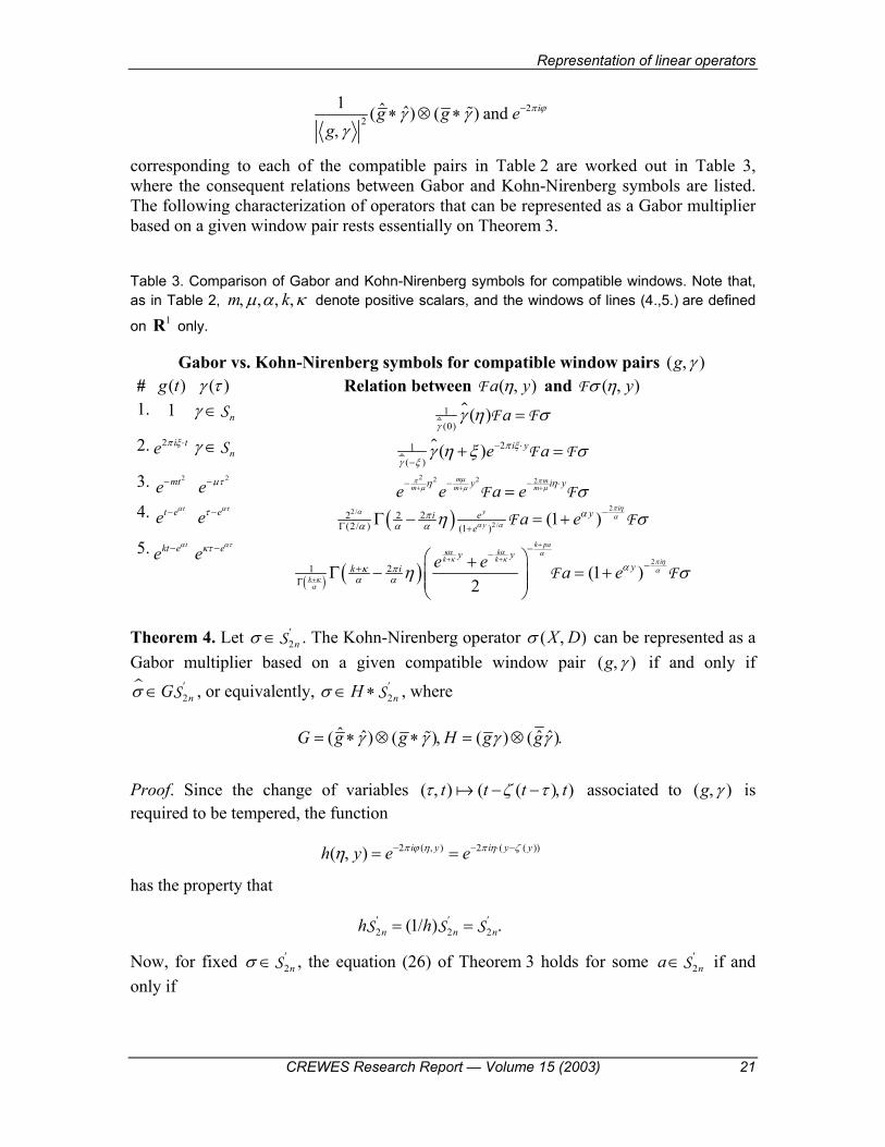
corresponding to each of the compatible pairs in Table 2 are worked out in Table 3, where the consequent relations between Gabor and Kohn-Nirenberg symbols are listed. The following characterization of operators that can be represented as a Gabor multiplier based on a given window pair rests essentially on Theorem 3.

Table 3. Comparison of Gabor and Kohn-Nirenberg symbols for compatible windows. Note that, as in Table 2, m kµ α κ, , , , denote positive scalars, and the windows of lines (4.,5.) are defined

on 1R only.

Gabor vs. Kohn-Nirenberg symbols for compatible window pairs ( )g γ, # ( )g t ( )γ τ Relation between ( )a yη,F and ( )yσ η,F 1. 1 nγ ∈S 1

(0)( ) a

γγ η σ=F F

2. 2 i te π ξ ⋅nγ ∈S 21

( )( ) i ye aπ ξ

γ ξγ η ξ σ− ⋅

−+ =F F

3. 2mte− 2

e µτ− 2 2 2 2m m

m m my i ye e a eµπ π

µ µ µη η σ+ + +− − − ⋅=F F 4. tt ee

α− eeαττ − ( )

22

222 2

(2 ) (1 )(1 )

iy

yyi e

ea e

π ηαα

α ααπ

α α α η σ/

/

−Γ / +

Γ − = +F F

5. tkt eeα− ee

ατκτ − ( ) ( )

221 (1 )

2

k pak

k k i

k

y yyk i e e a e

κα α ακ κ π η

ακ

α

ακ πα α η σ

+

+ +

+

−−−+

Γ

+Γ − = +

F F

Theorem 4. Let 2nσ ′∈S . The Kohn-Nirenberg operator ( )X Dσ , can be represented as a Gabor multiplier based on a given compatible window pair ( )g γ, if and only if

2nGσ ′∈ S , or equivalently, 2nHσ ′∈ ∗S , where

ˆ ˆ ˆ ˆ( ) ( ) ( ) ( )G g g H g gγ γ γ γ= ∗ ⊗ ∗ , = ⊗ .

Proof. Since the change of variables ( ) ( ( ) )t t t tτ ζ τ, − − , associated to ( )g γ, is required to be tempered, the function

2 ( ) 2 ( ( ))( ) i y i y yh y e eπ ϕ η π η ζη − , − ⋅ −, = =

has the property that

2 2 2(1 )n n nh h′ ′ ′= / = .S S S

Now, for fixed 2nσ ′∈S , the equation (26) of Theorem 3 holds for some 2na ′∈S if and only if



( )2 2 22

ˆ ˆ( ) ( ) ˆ ˆ ˆˆ( ) ( ) ( ) ( )n n ng g g g g g

g hγ γσ γ γ σ γ γ

γ′ ′ ′∗ ⊗ ∗

∈ = ∗ ⊗ ∗ ⇐⇒ ∈ ⊗ ∗ .,

F S S S

We can read off from this result some basic heuristic principles concerning the

existence of a Gabor multiplier based on given windows that represents a given Kohn-Nirenberg operator, as follows. In order to represent ( )X Dσ , as a Gabor multiplier

based on the compatible window pair ( )g γ, , it has to be the case that ( )yσ η, decays as fast as ˆ ˆg γ∗ in the variables η , and as fast as g γ∗ in the variables y . The symbol

( )xσ ξ, itself has to be as smooth as gγ in the variables x , and as smooth as ˆ ˆgγ in the variables ξ .

Theorem 4 shows that for Gabor multipliers based on a given window pair ( )g γ, to represent a wide class of linear operators, the function H should approximate a delta function, so that 2 2n nH ′ ′∗ ≅S S . Note that the scope of identical windows g γ= is limited

by the uncertainty principle: it is not possible for gγ and ˆ ˆgγ to both be highly localized, so the symbol ( )xσ ξ, of an operator representable using identical windows must be slowly varying in either x or ξ . This constraint can be avoided by using distinct windows g γ, , provided one of g γ, is highly localized while the Fourier transform of the other is highly localized. In keeping with this assertion, we will see in Section 3.5 that maximum generality is achieved with the “singular” window pair ( ) (1 )g γ δ, = , and its reversal ( 1)δ , .

Generality of Gaussian versus extreme value windows With respect to the realization of linear operators as Gabor multipliers, the generality

of a given window pair ( )g γ, is represented by the set

2 2( ) such that ( ) gn n aR g a X D γγ σ σ

′ ′ ,

, = ∈ ∃ ∈ , = .S S M

And so, given two window pairs 1 1( )g γ, , 2 2( )g γ, on nR , we say that 1 1( )g γ, is more general than 2 2( )g γ, if

2 2 1 1( ) ( )R g R gγ γ, ⊆ , ,

or equivalently, if

2 2 1 1( ) ( )R g R gγ γ, ⊆ , .

In terms to this notation, Theorem 4 says that for a compatible window pair on nR ,



2 2ˆˆ ˆˆ( ) ( ) ( ) and ( ) ( ) ( )n nR g g g R g g gγ γ γ γ γ γ′ ′, = ⊗ ∗ , = ∗ ⊗ ∗ ,S S

which allows us to compare the generality of any two compatible window pairs. For example, the next result shows that extreme value windows are more general than Gaussians.

Proposition 17. Let 0mα µ, , > be fixed. On 1R , the window pair

( )1 1( ) ( )t tt e t eg t t e e

α α

γ

− −, = ,

is more general than the window pair

( ) 2 2

2 2( ) ( ) mt tg t t e e µγ

− −, = , .

Proof. We carry out some computations so as to be able to apply Theorem 4. Write

1 1 1 1 1

2 2 2 2 2

( ) ( )( ) ( )

K g gK g g

γ γγ γ

= ∗ ⊗ ∗ ,= ∗ ⊗ ∗ .

From Table 3,

( )

22

2 21 1

2 2 2

22 2

21 2 21 (2 ) (1 )

12

( )

( )

iy

y

mm m

i eeg

y

g

K y

K y e e

π ηα α

α α

µπµ µ

πα α αγ

η

γ

η η

η

+

/

+ +

Γ / +,

− −

,

, = Γ − ,

, = .

Note that 1 2 1 2K K′ ′ ′=S S , where

( )

22

21 1

2

12 1

1 1(2 )

22(1 )

( ) ( )i

y

y

g

i ee

K y K yπ η

α α

α α

α γ

πα α

η η

η

+

/

−′

Γ / ,

+

, = ,

= Γ − .

And 2 2 2 2K K′ ′ ′=S S , where

2 2 2

2 222 2

1( ) ( )

mm m y

K y K yg

e eµπ

µ µη

η ηγ

+ +

′

− −

, = ,,

= .

We claim that 2 1 2K K′ ′/ ∈P , from which it follows that 2 1 2 2( )K K′ ′ ′ ′/ ⊆S S . To verify the claim, it suffices to compute the rate of decay of 1K ′ and to see that it is less than that of

2K ′ . By Stirling’s approximation this works out to be



22 1

2 ( )1( ) yK y e

πα α ηη η − − | |+| |′| , | | | ,∼

which is slower than the Gaussian decay of 2K ′ .

Now, let 2ρ ′∈S be arbitrary, and consider the distribution 2K ρ′ :

( )2 1 2 1 1 2( )K K K K Kρ ρ′ ′ ′ ′ ′ ′= / ∈ ,S

which proves that 2 2 1 2K K′ ′ ′ ′⊆S S , or equivalently 2 2 1 2K S K S′ ′⊆ . By Theorem 4, this shows that 1 1( )g γ, is more general than 2 2( )g γ, .

Singular windows The class of window pairs established in Definition 2 is useful because Gabor

multipliers based on them are well-defined irrespective of the Gabor symbol. We were thus free to carry out a somewhat general analysis, unencumbered by questions of interpretation or scope of validity of formulas. But if one is interested, not in a general analysis, but rather in studying particular operators such as, say, a specific type of pseudodifferential operator, then there is good reason to consider windows of a more general type. This comes of course at a price—Gabor multipliers based on more general windows may be well-defined only for a limited class of Gabor symbols, and one has to carry out some sort of ad hoc analysis to determine this class. We will consider a few particular examples of such “singular” windows. To begin, we establish the relevant definitions.

Definition 18. If ng γ ′, ∈S are such that one of the expressions g γ, or gγ , is well-defined and non-zero, but ( )g γ, is not a window pair in the sense of Definition 2, then we call ( )g γ, a singular window pair on nR .

Definition 19. We say that a singular window pair ( )g γ, on nR is compatible, and that g and γ are singular compatible windows, if there exist distributions 1 2 nG G ′, ∈S and a change of variables ( ) ( )v w tψ τ, = , (not necessarily tempered) with w t τ= − such that for every nx∈R , the equation

( ) ( 0) 1 2x x xT g T G Gψγ, ,⊗ = ⊗T

holds in the sense of distributions.

Perhaps the simplest way to obtain singular compatible windows is as limits of regular compatible windows. For instance, if kγ δ→ is an approximate identity, then the compatible pairs (1 )kγ, , which have a consistent change of variables, tend to the limit (1 )δ, . The pair (1 )δ, is indeed singular compatible, with accompanying functions

1 2 1G Gδ= , = and change of variables ( ) ( )t tψ τ τ τ, = , − . Note that, for every nϕ θ, ∈S ,



21 ( ) ( ) ( ) ( )ixV x V x e xπ ξ

δϕ ξ ϕ ξ θ ξ θ− ⋅, = , , = .

Thus

1 2 ixa a eδ π ξϕ θ θ ϕ, − ⋅, = , ⊗ .M (30)

Since 22

ixne π ξθ ϕ− ⋅ ⊗ ∈S , the equation (30) shows that the Gabor multiplier 1

aδ,M is well-

defined for every 2na ′∈S .

The Schwartz kernel of 1aδ,M may be computed directly from (30):

( )

2 2 12

12

2

ix ixe eπ ξ π ξθ ϕ θ ϕ

θ ϕ

θ ϕ

− ⋅ − ⋅ −

− ∗−

∗−

⊗ = ⊗

= ⊗

= ⊗ .

F

F T

T F

It follows that

12( )aK aδ,

−= .M T F (31)

(We could have alternatively applied the formula of Proposition 7 to obtain the same result.) The expression (31) is of course the Schwartz kernel of the Kohn-Nirenberg pseudodifferential operator having symbol a . That is, changing notation slightly so that σ denotes the Gabor symbol in place of a , we have:

Proposition 20. For every 2nσ ′∈S , 1 ( )X Dδσ σ, = ,M .

This result is of theoretical importance in that it shows Gabor multipliers to be completely general, at least once we allow singular windows. Applying Proposition 8 and the adjoint formula of Proposition 4 yields that

1 1aa

δ δ ∗, ,

=M M

for any 2na ′∈S . Thus ( 1)δ , too is a singular compatible pair which gives rise to a well-defined Gabor multiplier irrespective of the symbol. Although they are genuine examples of singular compatible windows, the pairs (1 )δ, and ( 1)delta, do not really give anything new, since Gabor multipliers based on them are just Kohn-Nirenberg operators (or their adjoints) in disguise.

On the other hand, if we let α tend to ∞ in the compatible pair

tkt e ee e

α ατκτ

− −,

on 1R , we obtain something new, namely the pair



( ( ) ( )) ( ) ( )ktg t H t e H eκτγ τ τ

, = − , − , (32)

where H denotes the Heaviside jump function and 0k κ, > are constants. The associated functions ( )

1( ) ( ) k vG v H v e κ+= − ,

( ( ) ( ))2

0( )

0

kwkH w H w w

w

e wG w e

e wκ

κ− −

−

≤= = ,

>

and the change of variables ( ) ( ) (max{ } )v w t t tψ τ τ τ, = , = , , − , verify that (32) conforms to the definition of a singular compatible window pair. By Proposition 7 the Gabor multiplier g

aγ,M based on the windows (32) has kernel

21

11

1( )ga GG

K N ag

γψγ

, −⊗= ,

,M T F F (33)

provided the latter is well-defined. A short calculation yields that

( ( ) ( ))21

1 ( )2

kH y H y yky eGGg k iκκη

γ κ π η− −+

⊗ , = ., + −

Note that ( ( ) ( ))kH y H y ye κ− − is not differentiable at 0y = , which implies that if ( )a yη, is singular at some point ( 0)η, then the usual distributional calculus breaks down for the right-hand side of (33). In this case the interpretation of g

aγ,M requires additional

clarification (which in practice can be quite straightforward).

We have already pointed out that for any nγ ∈S , the pair (1 )γ, is compatible, and hence so is its reversal ( 1)γ , . In dimension 1n = , a limiting case of the latter is the pair

( 1) ( ) ( ) tt H t eγ γ, , = − . (34)

The truncated exponential γ in the pair (34) is advantageous for a couple of reasons. Not only is it amenable to explicit calculation, but also the singularity at 0 renders the pair ( 1)γ , more general than if γ were a Schwartz class function, as we will now show. Note first that (34) is singular compatible with associated functions

1 2 1 ( ) ( )G G t t tγ ψ τ τ= , = , , = , − .

And the Gabor multiplier 1aγ ,M makes sense for arbitrary symbol 2a ′∈S . Furthermore,

12

1 221

1 1( )1 1 2

iy eGG iπ ϕ

ψη

γ π η −−

−⊗ , = , = ,, −

FT T F F

where ( )y yϕ η η, = . Thus if a Kohn-Nirenberg operator ( )X Dσ , can be represented as a Gabor multiplier 1

aγ ,M based on the windows (34), then by (27) the Gabor and Kohn-

Nirenberg symbols are related by the equation



21 ( ) ( )1 2

i ya y e yi

π ηη σ ηπ η

−, = ,−

F F

2( ) (1 2 ) ixa x i e π ξξ π ξ σ

⇐⇒ , = − ∗ . (35)

The equation (35) imposes no restrictions on σ for the existence of a corresponding Gabor symbol a . In other words, the window pair (34) is completely general:

2( ( ) 1)tR H t e ′− , = .S

SUMMARY The starting point for the present paper was the two-fold premise that (i) in practice

one often encounters linear operators in Kohn-Nirenberg form, ( )X Dσ , , and that (ii) it is of interest both from the numerical and analytical points of view to express such an operator as a Gabor multiplier g

a a gV N Vγγ

, ∗=M , for some choice of localizing windows g γ, . We have determined a class of window pairs, namely, compatible pairs and singular compatible pairs, for which there exists an explicit formula by which to compute the Gabor symbol a in terms of the given Kohn-Nirenberg symbol σ . More precisely, the ratio aσ/ of the Fourier transforms of the symbols is given in terms of the windows by the expression

2

2ˆ ˆ( ) ( )

ie g gg

π ϕ

γ γγ

∗ ⊗ ∗ ,,

(36)

where the phase function ϕ is

( ) ( )( )( )

gXgX yy ygg y

γγϕ η ηγγ

,∗, = ⋅ − − . ,∗

(37)

Extreme value windows are a particularly interesting example of compatible windows which are approximately causal (or reverse causal), and are more general than Gaussians with respect to the representation of linear operators. The class of singular compatible windows includes window pairs in terms of which every linear operator may be represented as a Gabor multiplier. Within this framework, the Kohn-Nirenberg formulation itself is an example of a Gabor multiplier, based on the singular window pair (1 )δ, . These results offer the prospect of investigating (or evaluating) particular linear operators, for example partial differential operators or nonstationary filters, in terms of their myriad representations as Gabor multipliers.

In conclusion we mention a couple of open problems stemming from the present paper. Concerning the formula (36) for the ratio of the transformed symbols, it is known to be valid for compatible and singular compatible windows. But are there other, non-compatible windows for which it is also valid? More generally, is there a broader class of window pairs, for which formulas analogous to (36) and (37) can be obtained?



REFERENCES [1] Hans G. Feichtinger and Krysztof Nowak, A first survey of Gabor multipliers, in Advances in Gabor

analysis, Hans G. Feichtinger and Thomas Strohmer, editors, Applied and Numerical Harmonic Analysis, Birkhäuser, Boston, 2003.

[2] R. A. Fisher and L. H. C. Tippett, Limiting forms of the frequency distribution of the largest or smallest member of a sample, Proceedings of the Cambridge Philosophical Society, XXIV Pt. 2 (1928), 180-190.

[3] Peter C. Gibson and Petr Zizler, Compatible windows in Gabor analysis (working title), in preparation. [4] Karlheinz Gröchenig, Foundations of time-frequency analysis, Applied and Numerical Harmonic

Analysis, Birkhäuser, Boston, 2001. [5] Michael P. Lamoureux, Peter C. Gibson, Jeff P. Grossman and Gary F. Margrave, A fast, discrete

Gabor transform via a partition of unity, 35pp., submitted to The Journal of Fourier Analysis and Applications.

[6] Gary F. Margrave and Robert J. Ferguson, Wavefield extrapolation by nonstationary phase shift, Geophysics, 64 (1999), 1067-1078.

[7] Gary F. Margrave, Robert J. Ferguson, and Michael P. Lamoureux, 2002, Approximate Fourier Integral Wavefield Extrapolators for Heterogeneous, Anisotropic Media, Canadian Applied Mathematics Quarterly, in press.

[8] Gary F. Margrave, Michael P. Lamoureux, Jeff P. Grossman, and V. Iliescu, Gabor deconvolution of seismic data for source waveform and Q correction, in 72nd Ann. Internat. Mtg, Soc. of Expl. Geophys., Expanded Abstract Volume, (2002), 2190-2193.

[9] Richard Rochberg and Kazuya Tachizawa, Pseudodifferential operators, Gabor frames, and local trigonometric bases, in Gabor analysis and algorithms: Theory and applications, Hans G. Feichtinger and Thomas Strohmer, editors, Applied and Numerical Harmonic Analysis, Birkhäuser, Boston, 1998.

[10] Laurent Schwartz, Théorie des noyaux, Proceedings of the International Congress of Mathematicians 1 (1950), 220–230.

representation of linear operators by gabor multipliers · representation of linear operators...

Documents