representations for understanding the stern …€¦ · representations for understanding the...
TRANSCRIPT
REPRESENTATIONS FOR UNDERSTANDING THE
STERN-GERLACH EFFECT
by
Jared Rees Stenson
A thesis submitted to the faculty of
Brigham Young University
in partial fulfillment of the requirements for the degree of
Master of Science
Department of Physics and Astronomy
Brigham Young University
August 2005

Copyright c© 2005 Jared Rees Stenson
All Rights Reserved

BRIGHAM YOUNG UNIVERSITY
GRADUATE COMMITTEE APPROVAL
of a thesis submitted by
Jared Rees Stenson
This thesis has been read by each member of the following graduate committee andby majority vote has been found to be satisfactory.
Date Jean-Francois S. Van Huele, Chair
Date Eric W. Hirschmann
Date Manuel Berrondo
Date David A. Grandy
BRIGHAM YOUNG UNIVERSITY
As chair of the candidate’s graduate committee, I have read the thesis of Jared ReesStenson in its final form and have found that (1) its format, citations, and biblio-graphical style are consistent and acceptable and fulfill university and departmentstyle requirements; (2) its illustrative materials including figures, tables, and chartsare in place; and (3) the final manuscript is satisfactory to the graduate committeeand is ready for submission to the university library.
Date Jean-Francois S. Van Huele,Chair, Graduate Committee
Accepted for the Department
Scott D. Sommerfeldt,Chair, Department of Physics and Astronomy
Accepted for the College
G. Rex Bryce,Associate Dean, College of Mathematicaland Physical Sciences

ABSTRACT
REPRESENTATIONS FOR UNDERSTANDING THE STERN-GERLACH
EFFECT
Jared Rees Stenson
Department of Physics and Astronomy
Master of Science
The traditional development of the Stern-Gerlach effect carries with it several
very subtle assumptions and approximations. We point out the degree to which this
fact has affected the way we practice and interpret modern physics. In order to gain
a more complete picture of the Stern-Gerlach effect we apply several techniques and
introduce the inhomogeneous Stern-Gerlach effect in which the strong uniform field
component is removed. This allows us to identify precession as a critical concept and
provide us with a mean to study it in a different and valuable context. Comparison
of the various techniques used gives us insight into the applicability of the standard
approximations and assumptions. This also provides the context for a more general
discussion regarding the use of representations in physics and teaching.

ACKNOWLEDGMENTS
Express appreciation here.

Contents
Acknowledgments vi
List of Tables ix
List of Figures xi
1 Introduction 1
2 On Representations in Physics 5
2.1 The Necessity of Representations . . . . . . . . . . . . . . . . . . . . 5
2.2 Mathematical Representations . . . . . . . . . . . . . . . . . . . . . . 7
2.2.1 Vectors and Rotations . . . . . . . . . . . . . . . . . . . . . . 8
2.2.2 Coordinate Systems . . . . . . . . . . . . . . . . . . . . . . . . 10
2.3 Conceptual Representations . . . . . . . . . . . . . . . . . . . . . . . 12
2.3.1 Conceptual Systems and Orthogonal Concepts . . . . . . . . . 13
2.3.2 The Early Scientific Revolution . . . . . . . . . . . . . . . . . 13
2.3.3 Wave-Particle Duality . . . . . . . . . . . . . . . . . . . . . . 15
2.4 Representations as Standards . . . . . . . . . . . . . . . . . . . . . . 17
3 A Thematic Account of the Stern-Gerlach Effect 19
3.1 The Classical Representation of the Stern-Gerlach Effect . . . . . . . 19
3.2 Quantum Mechanics . . . . . . . . . . . . . . . . . . . . . . . . . . . 23
3.2.1 Spin . . . . . . . . . . . . . . . . . . . . . . . . . . . . . . . . 26
3.2.2 Expectation Values . . . . . . . . . . . . . . . . . . . . . . . . 29
3.2.3 Measurement . . . . . . . . . . . . . . . . . . . . . . . . . . . 29
3.2.4 The Uncertainty Principle . . . . . . . . . . . . . . . . . . . . 30
vii

3.2.5 Stern and Gerlach’s Experiment . . . . . . . . . . . . . . . . . 31
4 A Historical Account of the Stern-Gerlach Effect 35
4.1 Atomic Models . . . . . . . . . . . . . . . . . . . . . . . . . . . . . . 35
4.1.1 1913: The Bohr Model . . . . . . . . . . . . . . . . . . . . . . 36
4.1.2 1916: The Sommerfeld Model . . . . . . . . . . . . . . . . . . 38
4.2 1921-1922: Stern and Gerlach’s Experiment . . . . . . . . . . . . . . 38
4.2.1 Magnet Type . . . . . . . . . . . . . . . . . . . . . . . . . . . 38
4.2.2 Particle Choice . . . . . . . . . . . . . . . . . . . . . . . . . . 39
4.2.3 Beam Width . . . . . . . . . . . . . . . . . . . . . . . . . . . 39
4.2.4 Results . . . . . . . . . . . . . . . . . . . . . . . . . . . . . . . 41
4.3 1925-1926: Quantum Mechanics . . . . . . . . . . . . . . . . . . . . . 41
4.4 1925: Spin . . . . . . . . . . . . . . . . . . . . . . . . . . . . . . . . . 42
4.5 1935: Measurement . . . . . . . . . . . . . . . . . . . . . . . . . . . . 43
5 Problems With Accounts of the Stern-Gerlach Effect 45
5.1 Problems from Quantum Mechanics . . . . . . . . . . . . . . . . . . . 45
5.1.1 Rightness and Clarity . . . . . . . . . . . . . . . . . . . . . . . 46
5.1.2 Representations as a Map . . . . . . . . . . . . . . . . . . . . 47
5.1.3 Communication . . . . . . . . . . . . . . . . . . . . . . . . . . 47
5.2 Problems with Historical Accounts . . . . . . . . . . . . . . . . . . . 48
5.3 Problems with Thematic Accounts . . . . . . . . . . . . . . . . . . . 49
5.3.1 An Artificial History . . . . . . . . . . . . . . . . . . . . . . . 49
5.3.2 Misunderstanding the Practical Aspects of the Stern-Gerlach
Effect . . . . . . . . . . . . . . . . . . . . . . . . . . . . . . . 51
5.4 The Magnetic Field . . . . . . . . . . . . . . . . . . . . . . . . . . . . 52
5.5 Precession Arguments . . . . . . . . . . . . . . . . . . . . . . . . . . 53
5.5.1 Classical Precession . . . . . . . . . . . . . . . . . . . . . . . . 54
5.5.2 Quantum Precession . . . . . . . . . . . . . . . . . . . . . . . 55
5.5.3 Precession and the Uncertainty Principle . . . . . . . . . . . . 58
viii

6 The Proposal 61
6.1 Positivist and Realist Representations . . . . . . . . . . . . . . . . . . 62
6.1.1 The Changing Role of Precession . . . . . . . . . . . . . . . . 63
6.2 Proposal: The Inhomogeneous Stern-Gerlach Effect . . . . . . . . . . 64
6.2.1 The Experimental Arrangement . . . . . . . . . . . . . . . . . 64
6.2.2 Possible Outcomes . . . . . . . . . . . . . . . . . . . . . . . . 66
7 A More Complete Study of the Stern-Gerlach Effect 67
7.1 Matrix Representation in a Moving Frame . . . . . . . . . . . . . . . 67
7.1.1 The Assumptions . . . . . . . . . . . . . . . . . . . . . . . . . 67
7.1.2 The Eigenstates . . . . . . . . . . . . . . . . . . . . . . . . . . 68
7.1.3 Demonstrating Precession . . . . . . . . . . . . . . . . . . . . 69
7.1.4 The Inhomogeneous Stern-Gerlach Effect . . . . . . . . . . . . 70
7.2 Position and Momentum Representations . . . . . . . . . . . . . . . . 71
7.3 Rotated and Unrotated Representations: Decoupling . . . . . . . . . 73
7.4 Cartesian and Polar Representations: Separation . . . . . . . . . . . 75
7.5 Series Solution Representation . . . . . . . . . . . . . . . . . . . . . . 76
7.5.1 Singularity Structure and Fuch’s Theorem . . . . . . . . . . . 76
7.5.2 The Indicial Equation . . . . . . . . . . . . . . . . . . . . . . 77
7.5.3 Recurrence Relation . . . . . . . . . . . . . . . . . . . . . . . 77
7.5.4 Extracting Behavior . . . . . . . . . . . . . . . . . . . . . . . 77
7.5.5 Truncation . . . . . . . . . . . . . . . . . . . . . . . . . . . . . 78
7.5.6 Radius of Convergence . . . . . . . . . . . . . . . . . . . . . . 79
7.5.7 Near-Origin Approximation . . . . . . . . . . . . . . . . . . . 79
7.6 The Confluent Heun Equation . . . . . . . . . . . . . . . . . . . . . . 81
7.7 Cliffor Representation . . . . . . . . . . . . . . . . . . . . . . . . . . 82
7.8 Green’s Function Representation . . . . . . . . . . . . . . . . . . . . 84
7.8.1 A Magnetic Field with Gaussian Fall Off . . . . . . . . . . . . 85
7.8.2 The Born-Approximation . . . . . . . . . . . . . . . . . . . . . 86
7.9 Schrodinger and Heisenberg Representations . . . . . . . . . . . . . . 87
ix
7.9.1 A Mixed Picture . . . . . . . . . . . . . . . . . . . . . . . . . 88
7.9.2 The Heisenberg Picture . . . . . . . . . . . . . . . . . . . . . . 90
7.10 Comment on Precession in the Inhomogeneous Stern-Gerlach Effect . 91
7.10.1 The Inhomogeneous Stern-Gerlach Effect as a Local Stern-Gerlach
Experiment . . . . . . . . . . . . . . . . . . . . . . . . . . . . 91
7.10.2 Making Precession Insignificant: A Semi-Classical Argument . 93
7.11 Other Representations . . . . . . . . . . . . . . . . . . . . . . . . . . 97
7.11.1 Propagators . . . . . . . . . . . . . . . . . . . . . . . . . . . . 97
7.11.2 Numerical Methods . . . . . . . . . . . . . . . . . . . . . . . . 98
7.11.3 Perturbation Theory . . . . . . . . . . . . . . . . . . . . . . . 98
7.11.4 Bohmian Mechanics . . . . . . . . . . . . . . . . . . . . . . . 98
8 Conclusions 101
8.1 The Method of Relativity . . . . . . . . . . . . . . . . . . . . . . . . 101
8.2 Our Results . . . . . . . . . . . . . . . . . . . . . . . . . . . . . . . . 102
8.3 The Dangers of an Inadequate Philosophy . . . . . . . . . . . . . . . 103
x

List of Tables
2.1 Relating Cartesian and Polar Coordinates . . . . . . . . . . . . . . . 11
2.2 Relating Cartesian and Polar Coordinates . . . . . . . . . . . . . . . 12
2.3 Wave and Particle Concepts . . . . . . . . . . . . . . . . . . . . . . . 16
5.1 Orthogonal Concepts . . . . . . . . . . . . . . . . . . . . . . . . . . . 46
xi

xii

List of Figures
2.1 The Cartesian Plane . . . . . . . . . . . . . . . . . . . . . . . . . . . 8
2.2 Vector Representations . . . . . . . . . . . . . . . . . . . . . . . . . . 9
2.3 Function Representations . . . . . . . . . . . . . . . . . . . . . . . . . 11
2.4 The Double Slit Experiment and Wave-Particle Duality . . . . . . . . 14
2.5 A Conceptual Coordinate System . . . . . . . . . . . . . . . . . . . . 15
3.1 The Classical Model of the Atom . . . . . . . . . . . . . . . . . . . . 20
3.2 Precession . . . . . . . . . . . . . . . . . . . . . . . . . . . . . . . . . 22
3.3 The Classical Representation of the Stern-Gerlach Effect . . . . . . . 23
3.4 Rotations in Physical and “Spin” Space . . . . . . . . . . . . . . . . . 27
4.1 The Bohr and Sommerfeld Atoms . . . . . . . . . . . . . . . . . . . . 37
4.2 A Representation of the Stern-Gerlach Apparatus . . . . . . . . . . . 40
4.3 Beam Cross Section and the Origial Stern-Gerlach Results . . . . . . 41
5.1 The Averaging of Components in Precession . . . . . . . . . . . . . . 55
6.1 The Inhomogeneous Magnetic Field . . . . . . . . . . . . . . . . . . . 65
6.2 Four Possible Outcomes for the Inhomogeneous stern-Gerlach Effect . 66
7.1 The Radial Separation of the Inhomogeneous Stern-Gerlach Effect . . 70
7.2 Rotating our Solutions in the Complex Plane . . . . . . . . . . . . . . 74
7.3 The Parameters for Finding a Constraint on the Observability of the
Precessionless Inhomogeneous Stern-Gerlach Effect . . . . . . . . . . 94
xiii

xiv

Chapter 1
Introduction
The early twentieth century was a defining time in physics. In fact, by the
mid-1900s a shift of ideas and methods had occurred on such a fundamental level
that the discipline of the late 1800s only vaguely resembled the discipline that would
close the next century. This shift was fueled by the wrestle between unexpected
experimental results and man-made theoretical notions. Amid all this, in 1921 Otto
Stern proposed one such experiment that not only validated the monumental shift
but helped give it form.
In the Stern-Gerlach experiment a beam of silver atoms was passed through
the poles of a magnet. Prior to this time the magnetic field may have been expected
to blur the beam into one continuous image due to the magnetic properties of the
atoms. However, a few years before it was carried out the idea had was proposed that
the magnetic properties of atoms would only manifest themselves in discrete values
upon measurement, not continuous ones. In a confirmation of this latest theory the
observed trace was indeed quantized. That is, the single beam of atoms did not blur
continuously but split into two distinct parts. This was a verification of the emerging
doctrine of quantization and, later, of the property of atomic spin.
Because of its simplicity and clarity the Stern-Gerlach experiment has now
become axiomatic in modern physics. It is often discussed in textbooks introducing
modern ideas and is taken as the clearest demonstration of the quantum measurement
process. However, as usually happens with axioms, it directed our study to such a
large degree that we seldom made it the object of our study.
1

Because it so clearly demonstrates quantization, entanglement, and measure-
ment - all of which are new quantum concepts - the canonization of the usual descrip-
tion of the Stern-Gerlach effect (SGE) has also canonized their usual interpretation.
The usual story of the SGE has gained clout however for good reason. It ties
the classical and quantum systems of thought. It seems to explain a clearly quantum
result in terms of almost purely classical concepts. For this reason we say it is clear.
For this reason it is also approximate.
It was our struggle to understand the classical-sounding story of the SGE in
quantum terms that led to this thesis. In the textbooks forces, trajectories, precess-
ing vectors were all used to make the description clear while on another page we
were forbidden to speak of such things in quantum descriptions (see citeGiffiths for
example).
Most of our difficulties seemed to be expressed in the phenomenon of precession
so our questions began with comparing its classical and quantum justifications. This
led to discussions of a more philosophical nature which in turn led to the interesting
discovery that sometimes a problem is too complex to solve singlehandedly. We
realized that a single problem could be presented, discussed, and solved in many
different ways. By comparing and contrasting these results we found ourselves using
a more experimental approach: we solved the same problem in various ways so as
to have a sufficient “sample” while only tweeking particular parts and maintaining
some “control” variables. After time, this lead to the formulation of our ideas on
representations.
Although they appeared last chronologically, we discuss these ideas on the
nature and value of representations in the next chapter. In our attempts to make
this a general discussion we use non-technical examples as well as technical ones.
The former we call Conceptual Representations and use them as examples of our
interpretational pictures in physics. The latter we call Mathematical Representations
which exemplify several of the solution methods used in later chapters. We relate
representations to the paradigms of [2] and discuss the consequence, both good and
bad, of canonizing a given representation.
2
Chapters 3 and 4 use the SGE to show how one phenomenon can be repre-
sented in two very different ways. The account of Chapter 3 emphasizes the logical
ordering of the concepts that are necessary to understanding the SGE from a quantum
perspective. For this reason it is called a Thematic Account and is often used in text-
books [1]. In contrast, we give a Historical Account in Chapter 4. Such an account is
characterized by its emphasis of the ordering of concepts and events chronologically.
Because the events of history are not always logical this is not as widely found in
teaching literature. However, in what follows we attempt to show that such accounts
do give an accurate picture of problem solving as the attempts of researchers are not
always logical either.
In the comparison of the approaches of Chapters 3 and 4 it will be seen how
taking either account as absolute can lead to problems. Chapter 5 discuss these
problems first in terms of the complementary relationship between rightness and
clarity. We show how most problems, both technical and philosophical, seem to
center on the phenomenon of precession and how the nature of precession depends
on the choice of magnetic field.
Having identified the source of most technical and interpretive problems in
Chapter 6 we outline a proposal to study the roles of both the magnetic field and
precession in the standard description of the SGE. This gives rise to what we call the
inhomogeneous SGE (ISGE). The remainder of this work is devoted to understanding
it.
In Chapter 7 we attempt to do this. Because of the tension between hav-
ing a clear account and a right account for the ISGE we choose to compare several
different representations and techniques for the problem. Among them are matrix rep-
resentations (section 7.1), differential calculus techniques (sections 7.2-7.6), Green’s
functions (section 7.8), and alternative representations for quantum mechanics such
as a the Cliffor (section 7.7), and Dirac (section 7.9) pictures. In section 7.11 we
suggest further approaches that could be used to arrive at a fuller understanding of
the ISGE.
3

In order to place these numerous and varied methods in an appropriate and
unifying context we begin with a discussion of the general role of representations.
4

Chapter 2
On Representations in Physics
Perhaps one of the most subtle aspects of learning to maneuver the physical
sciences is gaining an appreciation of and familiarity with representations. They
cannot be overly ostentatious or they would obscure the phenomenon of interest.
On the other hand, if they are too vague they fail to adequately communicate it.
As these two extreme cases are somewhat at odds with each other effectively using
various representations is tricky. This difficulty is compounded by our inability to
avoid them.
2.1 The Necessity of Representations
In order to express a rational statement it must be presented in a particular
way. That is, it must be given a representation so that it can be grasped by the
mind in terms of a concrete language and based on a set of familiar concepts. For
example, when we think of cars we do not have actual cars in our heads. We only
represent the concept of cars to our minds as thoughts. So we cannot just think but
we must think particular thoughts. In other words, because cars are not equivalent
to thoughts of cars a necessary process of translation takes place. We must therefore
constantly represent abstract concepts, either to our mind or to others’, in a particular
way. The specific manner in which a statement is expressed for its communication or
preservation in concrete form constitutes its representation. It is in this sense that
representations cannot be avoided.1
1For a development of similar ideas see [3] and [4] in which the process of conceptualization isdiscussed in detail. It is also pointed out that there are many levels of conceptualization, i.e. theperceptual, first order concepts, second order concepts, etc.
5

An analogous process occurs when translating between two languages. For
example, one might say,
(a) But look how the fish drink in the river.
or
(b) Pero mira como beben los peces en el rıo.
Using these two statements as different representations of the same idea we can learn
several things about representations in general.
(1) Representations are arbitrary in principle. Although (a) and (b) are very
different expressions they express exactly the same phenomenon.
(2) Representations make assumptions. (a) assumes a knowledge of the English
language while (b) assumes a knowledge of Spanish. Because assumptions can be more
or less general, representations occur simultaneously on different levels as well. Thus,
representations can be “layered” with the more specific ones occurring on top of more
general ones.
(3) Representations imply certain things. (a) implies that valid responses are
expressible in English whereas (b) implies that Spanish should be used. For spoken
languages this may be no surprise but in certain mathematical or physical situations
there may be problems or answers that are not easily expressible in a particular
way such as explaining the process of electron capture in an ancient African dialect,
describing quantum phenomena with only classical concepts, or using a discretely
indexed series to express a continuous process.
(4) Representations depend on cultural or philosophic values.2 Thus, they are
context dependent interpretations. To an English speaker (a) is a completely random
and detached observation whereas to a Spaniard (b), although describing an identical
phenomenon, brings to mind memories and scenes of a religious nature as it is a line
from a well known Christmas carol. It is in this sense that the selection and use of a
representation or interpretation is a necessary and unscientific part of physics.
2Conversely, cultural and philosophic values often depend on commonly accepted representationsand interpretations, e.g. the effects of Newtonian determinism and Darwinian evolution on religiousdiscourse. For this reason, we must be careful about how we represent science in society.
6
(5) Representations change the communicated meaning of the phenomenon
they describe. By utilizing attributes (1)-(4) above representations can be selected
to emphasize certain aspects, such as symmetries or biases, to our advantage. Un-
fortunately, they may also simultaneously and unintentionally obscure other aspects.
Making wise choices that properly balance this tradeoff is easily demonstrated but
near impossible to teach. This is because this choice is largely an intuitive or instinc-
tive process.3
These are only some of the characteristics of representations as we use the
term here. Other will be demonstrated shortly.
2.2 Mathematical Representations
Although there are many types of representations, perhaps as many as there
are languages, there are two that are of particular interest in the physics. They
might be categorized as mathematical and conceptual representations. The former
are typically thought of when representations are mentioned in scientific discourse
while the latter also play a very important, though less emphasized, role. We will
give a few examples to illustrate these two categories.
One of the earliest examples of a mathematical representation - after students
have mastered the ability to accept x as representing an unknown quantity - is the
use of the 2-dimensional cartesian grid. By drawing two intersecting lines we gain
the ability to express quantitative relationships which we say are 1-dimensional. The
choice however of which two lines is a choice of representation.
We often make the choice of using an “orthogonal” basis, that is, we choose
two lines that not only intersect but that are perpendicular to each other. The fact
that they are perpendicular usually provides us with a great simplification over non-
orthogonal axes. Also, note that if the information we were trying to represent were
more complex we could choose a higher dimensional space, e.g. more perpendicular
3An example of this might be making a judicious choice of coordinates in a Lagrangian problem.This ability seems to be the result of abstracting from experience and not from a concrete or deductiveprocess. As such, this process is not really taught but only repeatedly demonstrated by those whohave got the “hang of it.” Only some vague guidelines can be given as to how it is done.
7
x
y
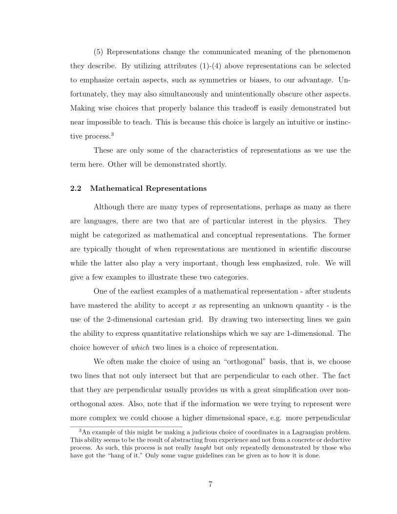
),( yx)(xy
Figure 2.1: On the 2-dimensional Cartesian plane any point can be represented as a couplet ofnumbers (x, y) specifying its relationship to a predetermined set of coordinate axes. Any set of thosepoints can be written as a function y(x).
axes, by which to represent them. If we were bound to only graphical representations
of coordinate systems such as in fig. 2.1 doing this for more than 2 or 3 dimensions
would be impossible but because of the more abstract algebraic representations of
Descartes’ analytic geometry we can easily write functions in n-dimensional spaces
as functions of n variables. We will however restrict ourselves to the simplest two-
dimensional examples.4
2.2.1 Vectors and Rotations
Suppose we have a vector in a 2-dimensional cartesian space. We often rep-
resent such an object as a directed line segment. The length of the line segment
quantitatively encodes the magnitude and its direction the orientation of the physical
quantity in question.
Leaving the vector in this graphical form requires that any mathematical op-
eration involving that vector be done in a graphical manner as well (see attribute (2)
above). Thus, we speak of placing vectors, head-to-tail and forming parallelograms,
etc. fig. 2.1(a) This is sometimes referred to as the coordinate free representation.
4Even when we discuss spin system we will restrict ourselves to 2-level systems for reasons dis-cussed in section 3.2.1.
8

A (b)
Ax
Ay
AAAAAA yyxxyx ˆˆ),( +==v BBBBBB yyxxyx ˆˆ),( +==v
(a) v
AB (c)
BxBy ϕ
Figure 2.2: (a) Vector v can be represented graphically as a directed line segment. In a graphicalmanner we can add other vectors to v by forming parallelograms. (b) By imposing an orthogonalcoordinate system A we can give our graphical representation a more compact algebraic form v =xAxA + yAyA. (c) If we rotate A to form a new coordinate system B the representation of v haschanged to v = xBxB + yB yB but the vector itself has not changed at all. Thus, some changes arisefrom the object itself while others arise only from the representation.
We can however use another layer of representation. If we create a set of
perpendicular coordinate axes with which to represent the vector it allows us to use
a more compact and general algebraic method to sum or multiply vectors. We are
therefore released from the limitations of the graphical methods we mentioned above.
If there were a reason to, we could and often do, arbitrarily rotate the coordi-
nate axes, perhaps to take advantage of a different symmetry. In doing so the length
and orientation of the vector are unaffected but its specific mathematical represen-
tation in the given basis would change since the axes are now tilted. Although the
9

components have changed the essential aspects of the vector have not and so any cal-
culation of physical results should be the same regardless of the choice of coordinate
system.
If the vector represents a quantity that is horizontal, such as a the displacement
of a ball rolling to the right on a table, we often choose to orient the coordinate axes
such that the displacement vector lies along the “x”-direction because this direction
is typically associated with the horizontal. This choice may reduce the complexity of
the problem to that of a 1-dimension (see attribute (5) above).
2.2.2 Coordinate Systems
Another example of a mathematical representation can be given which is of a
slightly different sort. Suppose we had two variables with a linear relationship. We
could represent it in a cartesian grid by writing
y = mx+ b, (2.1)
which is the familiar equation of a line with slope m and y-intercept b. This form
is simple and well known because it takes advantage of the linear symmetry of the
given line.
Likewise, if we were asked to represent a circle instead of a line we might have
chosen, based on the angular symmetry, a coordinate system that parameterized the
angle about the origin. In standard polar coordinates the circle is written as
r = a (2.2)
where a is the radius. Thus, taking advantage of the known symmetries allows us to
express relationships - lines and circles - in very simple ways.
However, if we weren’t as experienced with lines and circles or cartesian and
polar coordinates we might have chosen, perhaps based on some biased fancy, to ex-
press the line in polar and the circle in cartesian coordinates. Although this can be
done it disguises the problem in a messy representation. Their algebraic representa-
tions become
a = ±√x2 + y2, (2.3)
10

(a)
bx
y
(b)
ax
y
ϕ
rϕ
Figure 2.3: (a) Within a coordinate system described by the Cartesian coordinates (x, y) a line iseasily described. However, when described by standard polar coordinates (r, φ) its simple represen-tation is replaced by a non-linear equation. (b) Conversely, when a circle of radius a is representedit is easy in polar coordinates whereas it is more complicated in Cartesian form.
which is now a piecewise function, for the circle in cartesian coordinates and
r =b
sinϕ−m cosϕ, (2.4)
which is now non-linear, for the line in polar coordinates. Many more examples of
Cartesian Coordinates Polar Coordinates
line y = mx+ b r = bsin ϕ−m cos ϕ
circle a = ±√x2 + y2 r = a
Table 2.1: A table comparing Cartesian and Polar coordinate systems.
11

T ranslating Between Cartesian and Polar CoordinatesCartesian Coordinates ⇔ Polar Coordinates
x = r cosϕ r = ±√x2 + y2
y = r sinϕ ϕ = arctan(
yx
)Table 2.2: A table showing the transformation rules between the Cartesian and Polar coordinatesystems.
basis sets5, vector spaces, algebras6, coordinates systems, and representations7 could
be given.
These examples not only demonstrate interesting behaviors that properly be-
long to the representation and not to the curves themselves, i.e. the piecewise nature
of eq. (2.3), etc., but also the fact that representations can be layered, that is, you
may have representations of representations. This also shows that although the same
phenomenon can be given in various ways we often choose among the possibilities in
order to emphasize certain aspects. However, if we have no intuitive guide as to what
in the problem is worth emphasizing in the problem representations, even though
they can still be given, can be unnecessarily messy.
2.3 Conceptual Representations
Just as mathematical representations are utilized only when speaking math-
ematical languages conceptual representations must be used whenever concepts are
used. Their difference is demonstrated in the fact that while mathematics presupposes
certain concepts, e.g. numbers, concepts do not obviously presuppose a mathematical
language. In this way, conceptual representations can be seen to be more general than
5Basis sets can consist of many types of mathematical objects such as vectors, functions, matrices,etc. In fact, even real numbers can be thought of as a 1-dimensional space of which the basis set isthe number 1. That is, all numbers can be written as a linear combination of 1’s. Basis elementsare also usually chosen to be mutually orthogonal and normalized though they need not be.
6A specific algebra, the Clifford algebra, will be mention in Chapter 7.7Matrices, for example, require a particular representation.
12

mathematical ones. If this is the case then it follows that conceptual representations
are of extreme importance in physics, for math is. It also follows that selecting a
mathematical approach does carry conceptual consequences that may affect the ap-
proach and results of a problem.8 Indeed, specific instances of such representations
are used when we employ such things as models and interpretations, without which
science could not progress.9
A more suggestive term for all conceptual representations might be paradigms.
This is meant to allude to [2] which discusses at length the shaping role of paradigms
in science. We give shortly two specific examples of paradigm shifts.
2.3.1 Conceptual Systems and Orthogonal Concepts
Before giving some familiar examples of conceptual representations, or paradigms,
it is interesting to establish a paradigm of our own to show the similarities in form
with the mathematical ones given above. Just as in mathematics great utility is found
in representing objects in a coordinate system defined by certain basis elements, con-
ceptual pictures are formed in terms of their own basic set of components. In other
words, when a given concept can be explicitly identified as a particular weighted com-
bination of a few defining and elementary concepts, much as a vector can be described
in terms of its components within a coordinate system, great efficiency and progress
can be made. In this light, forming a paradigm is the qualitative equivalent to select-
ing an appropriate basis in which to describe phenomena. We will use this model in
the examples that follow.
2.3.2 The Early Scientific Revolution
A canonical example of a scientific paradigm shift is the early scientific revo-
lution that began with Copernicus and was consummated with Newton. We will not
8This addresses a very common opinion that is expressed whenever discussing the research topicof this thesis. Although mathematically “equivalent,” two methods may be markedly different interms of concepts or pedagogy.
9Although many downplay the importance of interpretations in physics today that little progresscan be made without them is especially manifest in the concerted efforts that went into formulatinga consistent interpretation of quantum mechanics in the first half of the last century. [5]
13

(a) (b)
Figure 2.4: (a) If a very low intensity beam of light is sent through a set of narrowly placedslits a pattern of dots accumulates one-by-one on the detecting screen. This is what we’d expect iflight were made up of particles. (b) However, if the beam is left for a long time or if the intensity isincreased so that several particles strike the scree we can see that the particles (photons) are strikingthe screen in an orderly fashion, i.e. in a series of bright and dark bands. Because this is exactlywhat we observe with all wave phenomena, such as with sound or water waves, this is what we’dexpect from if light were a wave. Therefore, we see that while the path of light is wave-like (as in(b)) the way in which it collides with detectors is particle-like (as in (a)).
go into the historical details but we can see that the change that occurred during
this time was primarily one of perspective. The gods had not altered their course,
neither had the planets changed their motion, and yet physics was revolutionized and
completely changed form. Simply put, before the revolution we operated in a concep-
tual “space” - a conceptual “coordinate” system - that set the concepts of simplicity,
anthropocentrism, and the duality of the terrestrial and divine natures among others
as the basis whereas after Copernicus, Kepler, Galileo, and Newton had done their
work we saw different advantages and accordingly shifted our values to one that en-
shrined objectivity, mechanism, reductionism, determinism, and mathematical rigor.
Our way of conceptualizing - of seeing problems - had been drastically altered. We
had effectively rotated or redefined our conceptual system so as to take advantage of
our new found values much as we did in section 2.1. As a result the way in which we
14
Wave
Particle
Some quantum phenomenonSome quantum phenomenon
Some classical phenomenonSome classical phenomenon
?
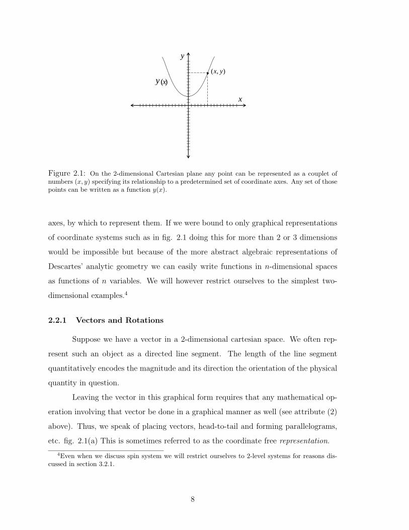
Figure 2.5: Because the duality demonstrated in the 2 slit experiment of fig. 2.4 is so commonin fully describing quantum phenomena we have realized the necessity of using a 2-dimensionalconceptual system. Each of the basis elements are classical concepts so only a 1-dimensional systemis needed to describe a phenomenon classically. We will see in section 3.2.4 that any representationin terms of these dual, or complementary, concepts is constrained to something like a circle, i.e. asa system is more describable in terms of particles it is correspondingly less describable in terms ofwaves. The question remains as to whether the phenomena themselves can evolve off the circle.
interpreted and categorized our problems, methods, results, and even values changed
as well.10
2.3.3 Wave-Particle Duality
There are more modern examples of paradigm shifts. One that has not resulted
in the final selection of one system completely at the expense of another, as did the
early scientific revolution, is couched in quantum mechanics.11 Here we have come to
grips with the need to adopt at least two very different paradigms. We have learned
to constantly shift our view between the two based on the nature of the questions
asked. This is because, in the language of mathematical spaces, our concepts have
been reduced to not just any set of concepts but to what we might call an orthogonal
10For an account of this period and an idea of the concepts that formed the conceptual “space”in which these theories developed see [6] or [7].
11See [8] for an excellent discussion of the history and development of many oddities in quantummechanics including wave-particle duality.
15
set of concepts. Bohr called these sorts of concepts “complementary” and developed
many ideas based on the principle of complementarity. [19] Similar to the definition
given in section 2.1 by orthogonal concepts we mean two concepts that are in no way
expressible in terms of each other. If we take light, for example, as our object of
description these two concepts are waves and particles.
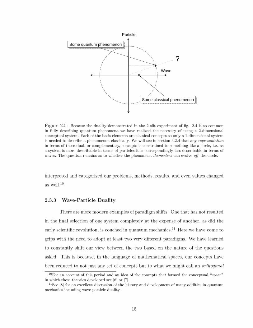
Particle Concepts Wave Concepts
Mass FrequencyTrajectory AmplitudeCollisions PhasePosition Wave FrontsForce Peaks
Table 2.3: A table of some concepts that we use to describe wave and particles. Particle conceptsare not well defined when applied to waves and visa versa. The set of concepts listed in either columnseparately form a conceptual space or basis, much as the set (x, y, z) does, within which the overallconcept of “particle” or “wave” can be clearly used.
Some experiments show light to demonstrate the properties of waves while
others demonstrate the properties of particles. Because there are at least these two
orthogonal ways of representing light there are at least two completely different sets of
properties of which we can learn. As a particle, we can use the well-defined concepts
of position, speed, mass, trajectory, and force as applied to light while as a wave we
may use wavefronts, interference, crests, troughs, frequency, and amplitude. It seems
that depending on the precise experimental questions we ask we may use either the
attributes and concepts of waves or particles in studying light.
It is interesting to note that we have effectively doubled the space in which
we describe quantum mechanics by doubling the the number of concepts that can be
applied to it. This is the reverse of the vector example above in which we chose a
mathematical representation so as to reduce the dimensionality of the problem. Here
16

we choose a conceptual representation that increases the conceptual dimensionality
of the problem in order to give it a more complete representation; the problem can
now be described as some combination of “waviness” and “particle-ness” just as a
vector might be describable in its x and y orthogonal components. This is not only
analogous to the introduction of spin into quantum mechanics into which the spin
degree of freedom was added in order to account for observed phenomena but it is
gist of the entire approach of this work. We attempt to expand the conceptual space
available to describing spin phenomena as manifest in the Stern-Gerlach effect. This
demonstrates the practical effects a shift in conceptual representation may have.
2.4 Representations as Standards
When the utility of a particular representation is demonstrated with respect
to a shared value system, whether mathematical or conceptual, they can become
standard, or axiomatic. As such, new hypotheses and results are compared against it
in order to gauge their validity and “truthfulness.” If there is an inconsistency it is the
nature of the hypothesis or result that is usually questioned and not the standard.12
This can have several undesirable consequences some of which are
(1) Their democratically-decided status as “standard” implies to many minds
the absolute status of unquestionable.
(2) Once considered standard the necessity and prevalence of representations
can easily be mistaken for complete objectivity.
(3) The characteristics of nature that they assume are seen as naturally or
mathematically imposed.
(4) The implications and emphases of the representation become confused with
those of the original phenomena.
(5) The solution methods and interpretations natural to the representation are
seen as required.
12When enough discrepancies arise there may come a point when the standards themselves beginto be questioned. This occurs at the onset of scientific revolutions. [2]
17
(6) The value system used to determine it and that arises from it are mistaken
as absolute.
In short, all unscientific aspects of the representation process can easily and
mistakenly be given scientific status. When they thus become axiomatic representa-
tions they are then often taken for granted and much valuable insight is lost.
On the other hand, standards and established norms - even to the hiding
of irregularities and messiness - are crucial to the communication and development
of any science. Therefore, sifting these subtleties out scientifically, not necessarily
abandoning them, is necessary for further progress.
18
Chapter 3
A Thematic Account of the Stern-Gerlach Effect
Representations come in many forms. They may be qualitatively expressed
in everyday language or quantitatively expressed in mathematical form. In any case,
a particular representation is chosen in order to emphasize a particular aspect of
the phenomenon being described. In this chapter we choose to represent the Stern-
Gerlach effect (SGE) in a manner that will appear very similar to those given in
various textbooks (see [1] or [9]). We will seek to emphasize the logical ordering of
the themes and concepts of the SGE in order to provide a clear and rational account.
For this reason we call it a thematic account. In the next chapter the same story will
be told but from a historical perspective.
3.1 The Classical Representation of the Stern-Gerlach Effect
We begin with a classical description of the SGE because it introduces the
main concepts with which students are usually familiar when it is first presented. It
therefore provides an appropriate context for the quantum mechanical “textbook”
description we subsequently give.
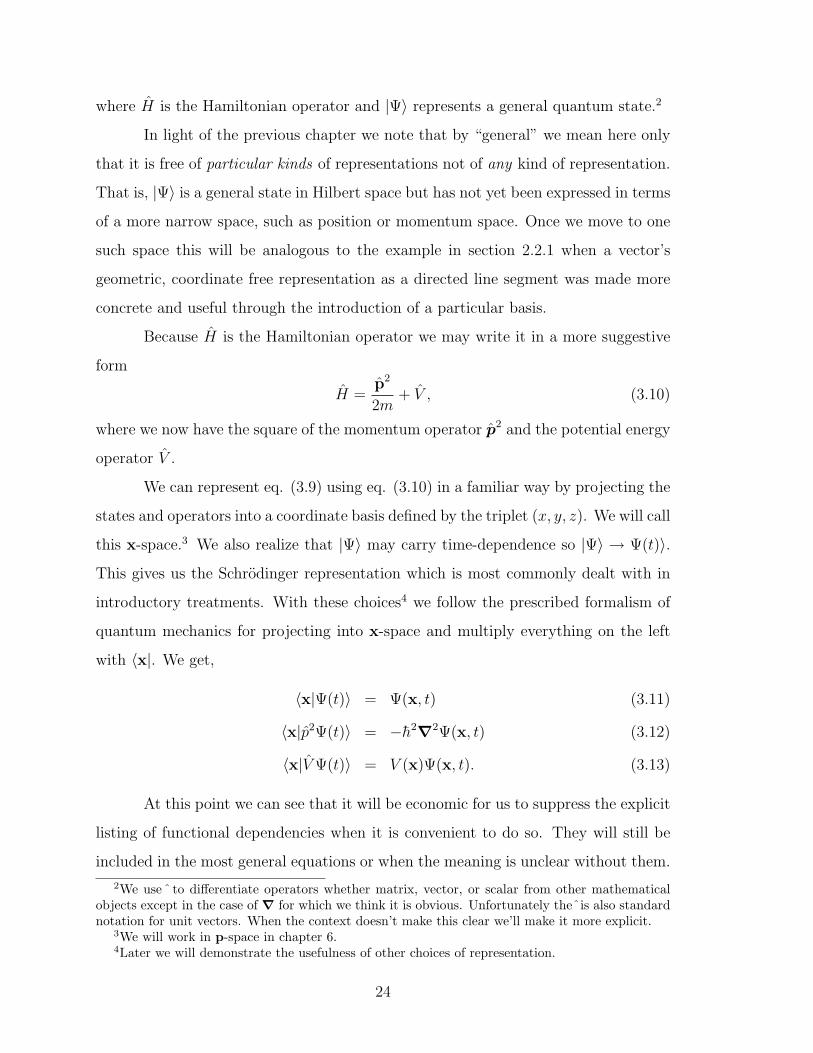
In the classical picture of the atom we treat the electron as tracing a definite
orbit around the nucleus. This moving charge creates a current I that encloses a
vector area A, with direction n normal to the surface in a righthanded sense with
the orbital motion. We may thus use the familiar equation for magnetic moments µ
from classical electromagnetic theory
µ = IA. (3.1)
19

empv =
L
nucleus
electron
ra ˆ=r
Figure 3.1: In the classical picture of the atom the electron orbits the nucleus much as a planetwould orbit the sun. Because it has a continuous set of definite trajectories with velocity v andmomentum p= mev there is a definite and continuous orbital angular momentum L= mr×v.
More specifically, if we assume that charge e orbits κ times1 around a circular path
of radius a with velocity v such that the period T of the particle is T = 2πa/v we
may write I = κe/T = κev/2πa. Using A= πa2n we have
µ =κeavn
2. (3.2)
Multiplying and dividing by the mass m of the particle allows us to recognize the
total angular momentum L= amvn. We now have a general magnetic moment
µ =κe
2mL (3.3)
for electrons. In the classical picture we assume that the particle carries the charge
so, since in one period T the particle makes one complete revolution, so does the
charge. Classically we take κ = 1. The reason for introducing κ will become more
apparent in section 3.2.1.
The energy of µ in a magnetic field B is
U = −µ ·B (3.4)
1Usually µ is derived classically without any mention of κ, since it is 1. We use this approachhere, which is not at all standard, to show two things. However we leave this discussion to section3.2.1.
20

and the dynamics are defined by
F = −∇U = ∇(µ ·B) and τ =dL
dt= µ×B. (3.5)
Using eq. (3.3) inverted for L and defining a characteristic frequency ω ≡ −κeB/2m
the second of these equations becomes
dµ
dt= ω × µ. (3.6)
Thus, as can be seen in fig. 3.2, the particle’s magnetic moment precesses about B
at a frequency ω.
As this aspect of the dynamics evolves the force equation also has an effect.
Under the very common though very subtle assumption that µ does not vary in space
the gradient operator in F of eq. (3.5) moves past µ giving the components, in index
notation, Fj = µk∂jBk. Therefore, the magnitude of the force felt by the particle will
be proportional to both the magnitude of µ and of ∇B as well as orientation of µ
relative to the field. The direction of F arises from the direction of the field gradient.
This means that the particles will sift themselves out according to the magnitude and
direction of their respective magnetic moments as they precess. The magnitude of
the deflection depending on the magnitude of µ in the direction of the field gradient
and the direction of the deflection being only a function of µ’s local direction. Said
differently, the fact of deflection reflects only the orientation of µ with respect to a
chosen field configuration while the direction of deflection communicates information
about the particle’s position in the field.
In order to classically derive the SGE we imaging passing a beam of particles
each with a random magnetic moment µ through a magnetic field that incorporates
both characteristics of interest: a field gradient b that induces deflections and a
uniform part that directs them a certain way. The simplest choice is
B = (B0 + bz)z. (3.7)
Applying this to eq. (3.5) yields
F = µbz (3.8)
21

Bω∝
μdtdμ
0θ
Figure 3.2: The vector µ will move in a direction that is perpendicular to both itself and themagnetic field direction B. As it thus moves its orientation changes. At every point µ will tend tomove in a direction tangent to the circle centered on and perpendicular to B. Thus, µ rotates orprecesses about B at a frequency of ω. Note that if there were some dissipative force in this systemµ would align with B as it precessed. This is what happens to a compass needle because of thefriction of the pivot point.
as the equation of motion. Thus, in the classical representation of the experiment
we expect each particle to move under a force that is proportional to µ and the field
gradient b in the direction of ∇B. Inasmuch as the orientation of µ is continuous
and ∇B is unidirectional a continuous, linear distribution of particles will register
on a detecting plate placed some distance behind the magnet. This is the classical
description of the SGE.
22

beam
Figure 3.3: A beam of atoms, whose magnetic properties can be represented as tiny bar magnets,enters an inhomogeneous magnetic field from the left. Depending upon the orientation of the barmagnetic in the field a net force will be exerted. This force causes a corresponding separation of thetrajectories.
3.2 Quantum Mechanics
The quantum description of this experiment is much different. Before going
into its derivation specifically a thematic approach requires that we introduce some
concepts that will be needed but that are not part of the classical intuition we have
built up. Together with the classical concepts, these will form a common conceptual
context from which students seeing the SGE for the first time will draw.
The governing equation of quantum mechanics is Schrodinger’s equation. In
general form it is
ih∂
∂t|Ψ〉 = H|Ψ〉 (3.9)
23
where H is the Hamiltonian operator and |Ψ〉 represents a general quantum state.2
In light of the previous chapter we note that by “general” we mean here only
that it is free of particular kinds of representations not of any kind of representation.
That is, |Ψ〉 is a general state in Hilbert space but has not yet been expressed in terms
of a more narrow space, such as position or momentum space. Once we move to one
such space this will be analogous to the example in section 2.2.1 when a vector’s
geometric, coordinate free representation as a directed line segment was made more
concrete and useful through the introduction of a particular basis.
Because H is the Hamiltonian operator we may write it in a more suggestive
form
H =p2
2m+ V , (3.10)
where we now have the square of the momentum operator p2 and the potential energy
operator V .
We can represent eq. (3.9) using eq. (3.10) in a familiar way by projecting the
states and operators into a coordinate basis defined by the triplet (x, y, z). We will call
this x-space.3 We also realize that |Ψ〉 may carry time-dependence so |Ψ〉 → Ψ(t)〉.
This gives us the Schrodinger representation which is most commonly dealt with in
introductory treatments. With these choices4 we follow the prescribed formalism of
quantum mechanics for projecting into x-space and multiply everything on the left
with 〈x|. We get,
〈x|Ψ(t)〉 = Ψ(x, t) (3.11)
〈x|p2Ψ(t)〉 = −h2∇2Ψ(x, t) (3.12)
〈x|VΨ(t)〉 = V (x)Ψ(x, t). (3.13)
At this point we can see that it will be economic for us to suppress the explicit
listing of functional dependencies when it is convenient to do so. They will still be
included in the most general equations or when the meaning is unclear without them.
2We use ˆ to differentiate operators whether matrix, vector, or scalar from other mathematicalobjects except in the case of ∇ for which we think it is obvious. Unfortunately theˆis also standardnotation for unit vectors. When the context doesn’t make this clear we’ll make it more explicit.
3We will work in p-space in chapter 6.4Later we will demonstrate the usefulness of other choices of representation.
24

Inserting these specified forms into eq. (3.9) we get
ih∂
∂tΨ = − h2
2m∇2Ψ + VΨ. (3.14)
This is the time-dependent Schrodinger equation represented in x-space.
Because this is now represented as a familiar differential equation we can use
familiar differential solution techniques to proceed. If H is time-independent, which
implies that V is as well, we can use the separation of variables technique to separate
the time behavior out. Assuming
Ψ(x, t) = ψ(x)T (t) (3.15)
and calling the constant of separation E yields the two equations
ET = ihd
dtT (3.16)
Eψ = − h2
2m∇2ψ + V ψ (3.17)
for the time and space parts respectively. Note that the spatial equation is an eigen-
value equation of the form
Hψn = Enψn (3.18)
with eigenvalues En corresponding to eigenfunctions ψn and also that the partial time
derivative in eq. (3.16) can become a total derivative because of the lack of spatial
dependence in T . We will suppress the index n for now.
Solving the time piece gives
T (t) = T (0)e−ih
Et. (3.19)
A general solution of the full equation is then the linear combination
Ψ(x, t) =N∑
n=0
ψn(x)e−ih
Ent (3.20)
where N , the dimensionality of the quantum space, could be either finite or infinite.
All constants have been absorbed into ψn(x).
Had we represented our operators as N -dimensional matrices instead of alge-
braic operators we could have arrived at the same result. This would be a useful
choice for systems of only a few dimensions such as spin systems.
25
3.2.1 Spin
Spin is a necessary form of angular momentum in the quantum description
of nature. It is analogous to the classical orbital angular momentum L although it
has not yet been consistently associated with a conceptual picture of any spinning or
orbiting object. Orthodox interpretations of quantum mechanics take it to have no
classical manifestation and to be intrinsic to quantum objects such as photons and
electrons.
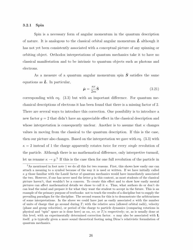
As a measure of a quantum angular momentum spin S satisfies the same
equations as L. In particular,
µ =κe
2mS (3.21)
corresponding with eq. (3.3) but with an important difference. For quantum me-
chanical descriptions of electrons it has been found that there is a missing factor of 2.
There are several ways to introduce this correction. One possibility is to introduce a
new factor g = 2 that didn’t have an appreciable effect in the classical description and
whose interpretation is consequently unclear. Another is to assume that κ changes
values in moving from the classical to the quantum description. If this is the case,
then our picture also changes. Based on the interpretation we gave with eq. (3.3) with
κ = 2 instead of 1 the charge apparently rotates twice for every single revolution of
the particle. Although there is no mathematical difference, only interpretive turmoil,
let us rename κ→ g.5 If this is the case then for one full revolution of the particle in
5As mentioned in foot note 1 we do all this for two reasons. First, this shows how easily one canattach a meaning to a symbol because of the way it is used or written. If we have initially calledκ g those familiar with the Lande factor of quantum mechanics would have immediately associatedthe two. However, if one has never used the letter g in this context, as most students of the classicalpicture haven’t, that wouldn’t be a concern. To create this effect and to show how easily mentalpictures can affect mathematical details we chose to call it κ. Thus, what authors do or don’t docan lead the mind and prepare it for what they want the student to accept in the future. This is anexample of the primary purpose of textbooks: not to teach the results of a discipline but to supply theprevailing paradigm for the discipline. The second reason for this is to demonstrate the arbitrarinessof some interpretations. In the above we could have just as easily associated κ with the numberof units of charge that go around during T ; with the relative area (allowed orbital radii), velocity(phase and group velocities), or period of the charge to particle dynamics (comparing rotations inphysical and “spin” space as is done here) as κa, κv, or T/κ respectively; or, as is usually done atthis level, with an experimentally determined correction factor. κ may also be associated with Litself. g is typically given a more sound theoretical footing using Dirac’s relativistic formulation ofquantum mechanics.
26

its orbit, described by L, there is only half a rotation of the charge that determines
µ and corresponds to S. As it turns out, the fact that one full rotation in physical
space corresponds to just half a rotation in spin space is exactly the result of other
theoretical spin descriptions.
(a)
3-dimensional Physical Space 2-dimensional “Spin” Space
⎟⎟⎠
⎞⎜⎜⎝
⎛01
~“up”
“down”
(b)
⎟⎟⎠
⎞⎜⎜⎝
⎛10
~
“down”
z+
z−
“up”
x−
x+
y−y+
⎟⎟⎟
⎠
⎞
⎜⎜⎜
⎝
⎛
100
~
⎟⎟⎟
⎠
⎞
⎜⎜⎜
⎝
⎛
−100
~
Figure 3.4: (a) Rotations of 180◦ in the familiar 3-dimensional, physical space correspond torotations of only 90◦ in “spin” space. That is, the “up” and “down” directions in z are 180◦ apartin physical space but because they can completely describe all the possible outcomes of a spin-zmeasurement they completely span the space describing spin properties. Thus they can be thoughtof as an orthogonal basis of this space.
Also, in contrast with classical measures of angular momentum, S can take
on only 2s + 1 discrete values where s is the quantum number defining the spin
characteristics of a system. For example, a measurement of the spin of the electron,
for which s = 1/2, in a given direction can only result as spin “up” or spin “down” in
27
that direction.6 Due to its two-valuedness, single electron spin systems are two-level
systems. These are extremely useful for modelling more complicated systems of more
states because they are the simplest systems that incorporate both the properties
of a single state with the phenomenon of transitions between states. Consequently,
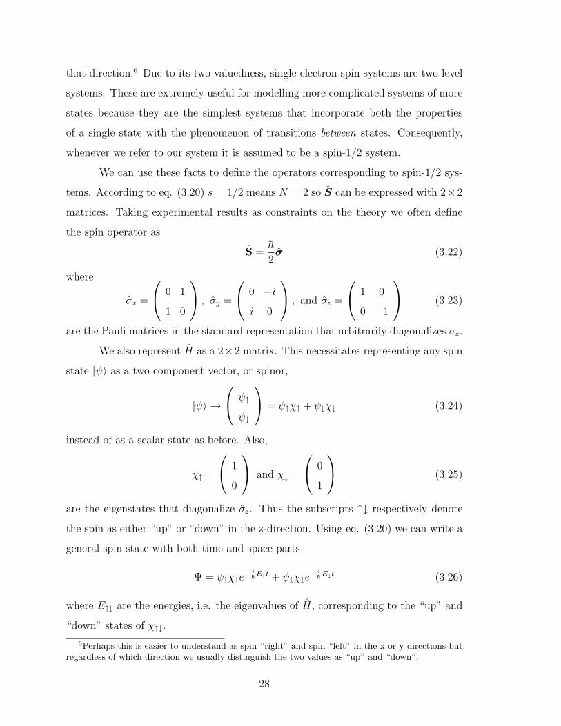
whenever we refer to our system it is assumed to be a spin-1/2 system.
We can use these facts to define the operators corresponding to spin-1/2 sys-
tems. According to eq. (3.20) s = 1/2 means N = 2 so S can be expressed with 2×2
matrices. Taking experimental results as constraints on the theory we often define
the spin operator as
S =h
2σ (3.22)
where
σx =
0 1
1 0
, σy =
0 −i
i 0
, and σz =
1 0
0 −1
(3.23)
are the Pauli matrices in the standard representation that arbitrarily diagonalizes σz.
We also represent H as a 2×2 matrix. This necessitates representing any spin
state |ψ〉 as a two component vector, or spinor,
|ψ〉 →
ψ↑
ψ↓
= ψ↑χ↑ + ψ↓χ↓ (3.24)
instead of as a scalar state as before. Also,
χ↑ =
1
0
and χ↓ =
0
1
(3.25)
are the eigenstates that diagonalize σz. Thus the subscripts ↑↓ respectively denote
the spin as either “up” or “down” in the z-direction. Using eq. (3.20) we can write a
general spin state with both time and space parts
Ψ = ψ↑χ↑e− i
hE↑t + ψ↓χ↓e
− ih
E↓t (3.26)
where E↑↓ are the energies, i.e. the eigenvalues of H, corresponding to the “up” and
“down” states of χ↑↓.
6Perhaps this is easier to understand as spin “right” and spin “left” in the x or y directions butregardless of which direction we usually distinguish the two values as “up” and “down”.
28

3.2.2 Expectation Values
Important in any theoretical treatment of quantum measurements is the con-
cept of expectation values. For a given state |ψ〉 every operator A has an expectation
value
〈A〉 ≡ 〈ψ|A|ψ〉. (3.27)
Using the specific case that A = x Griffiths [1] explains
[This] emphatically does not mean that if you measure the position of
one particle over and over again, [〈x〉] is the average of the results...Rather,
〈x〉 is the average of measurements performed on particles all in the state
ψ, which means you must find some way of returning the particle to
its original state after each measurement, or else you prepare a whole
ensemble of particles, each in the same state ψ, and measure the positions
of all of them: 〈x〉 is the average of these results (p. 14).
Discussing this further Griffiths [1] continues
this time in terms of velocity d〈x〉/dt, “Note that we’re talking about
the ‘velocity’ of the expectation value of x, which is not the same thing as
the velocity of the particle (p. 15).
With these statements we see that expectation values are averages of repeated mea-
surements on identical systems not of repeated measurements on a single system.
3.2.3 Measurement
As one can see, measurement plays a significant role in both our practice and
interpretation of quantum mechanics. There is however much ambiguity and debate
as to what exactly the process of measurement entails. In attempts by Bohr, Von
Neumann, Wigner, and others to clarify the ontological and/or epistemological nature
of these issues some unfamiliar concepts such as the unpredictable “collapse” of the
29

wave function or the placement of a “cut” between the quantum and classically de-
scribed worlds have been introduced.7 In what might be called the orthodox opinion
“Observations not only disturb what is to be measured, they produce it...[When mea-
suring position] we compel [the particle] to assume a definite position.” (Jordan in [1])
However, because of the proliferation of the ambiguous and unfamiliar ideas of the
“cut” and “collapse” there is only a quasi-standard conception of what measurement
is.
Because the SGE is considered the simplest and most clear demonstration of
the measurement of quantum phenomena as opposed to classical expectations it is
usually taken as the the canonical, or defining, example of the process of quantum
measurement.
3.2.4 The Uncertainty Principle
Another characteristic of quantum mechanics that must be brought up, and
which we will bring up, in the discussion of measurement and the SGE is the uncer-
tainty principle as formulated by Werner Heisenberg. It simply states that for a set
of non-commuting operators, say x and px, whose commutator is
[x, px] = xpx − pxx = ih (3.28)
the relation can be given
∆x∆px ≥h
2. (3.29)
where the square uncertainty of a particular measurement A is
∆A2 = 〈A2〉+ 〈A〉2. (3.30)
This is usually interpreted to mean that there is an irreducible uncertainty
associated with the simultaneous measurements of x and px. In other words, the more
confident we are of the result of a measurement of the position x of a particle, i.e.
smaller ∆x, the less certain we are of a simultaneous measurement of its momentum
7For a standard discussion of measurement see [10]. For an expression of some concerns involvedin these issues see [11] or [12].
30
in that same direction px, i.e. ∆px increases. To what extent this is an ontological or
epistemological principle is unclear.8
Of particular interest to our discussion here is the realization that the opera-
tors, denoting measurements of the three orthogonal spin directions Sx, Sy, and Sz,
do not mutually commute. Their simultaneous existence as well defined quantities is
therefore constrained by
[Si, Sj] = iεijkSk. (3.31)
More specifically, in any conceivable observation of the SGE no two components of
the spin will ever be specified with more certainty than eq. (3.31) allows.
3.2.5 Stern and Gerlach’s Experiment
Now that we have built up concepts relevant to the quantum representation
of the SGE we can outline what might be its typical quantum derivation [9]. Such a
derivation usually proceeds with the intent of making as few changes as possible to
the classical account.
There are some stark differences however. For example, there is no widely
accepted or technically defined concept of force in quantum mechanics, such as a
force operator, so our approach to the SGE must be given in terms of quantum
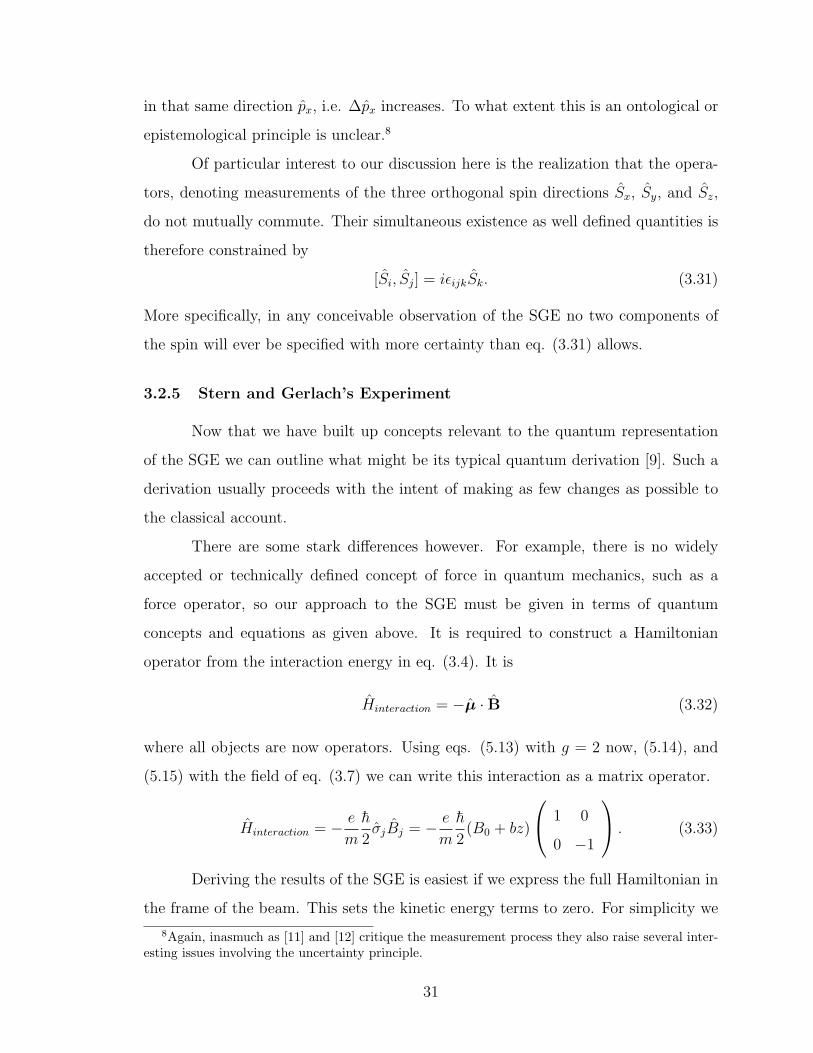
concepts and equations as given above. It is required to construct a Hamiltonian
operator from the interaction energy in eq. (3.4). It is
Hinteraction = −µ · B (3.32)
where all objects are now operators. Using eqs. (5.13) with g = 2 now, (5.14), and
(5.15) with the field of eq. (3.7) we can write this interaction as a matrix operator.
Hinteraction = − e
m
h
2σjBj = − e
m
h
2(B0 + bz)
1 0
0 −1
. (3.33)
Deriving the results of the SGE is easiest if we express the full Hamiltonian in
the frame of the beam. This sets the kinetic energy terms to zero. For simplicity we
8Again, inasmuch as [11] and [12] critique the measurement process they also raise several inter-esting issues involving the uncertainty principle.
31
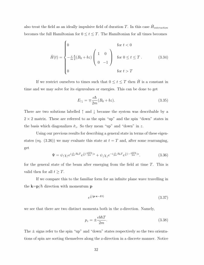
also treat the field as an ideally impulsive field of duration T . In this case Hinteraction
becomes the full Hamiltonian for 0 ≤ t ≤ T . The Hamiltonian for all times becomes
H(t) =
0 for t < 0
− em
h2(B0 + bz)
1 0
0 −1
for 0 ≤ t ≤ T
0 for t > T
. (3.34)
If we restrict ourselves to times such that 0 ≤ t ≤ T then H is a constant in
time and we may solve for its eigenvalues or energies. This can be done to get
E↑↓ = ∓ eh
2m(B0 + bz). (3.35)
There are two solutions labelled ↑ and ↓ because the system was describable by a
2 × 2 matrix. These are referred to as the spin “up” and the spin “down” states in
the basis which diagonalizes σz. So they mean “up” and “down” in z.
Using our previous results for describing a general state in terms of these eigen-
states (eq. (3.26)) we may evaluate this state at t = T and, after some rearranging,
get
Ψ = ψ↑χ↑ei e2m
B0T eih( ebTh
2m)z + ψ↓χ↓e
−i e2m
B0T eih(− ebTh
2m)z. (3.36)
for the general state of the beam after emerging from the field at time T . This is
valid then for all t ≥ T .
If we compare this to the familiar form for an infinite plane wave travelling in
the k=p/h direction with momentum p
eih(p·x−Et) (3.37)
we see that there are two distinct momenta both in the z-direction. Namely,
pz = ±ebhT2m
. (3.38)
The ± signs refer to the spin “up” and “down” states respectively so the two orienta-
tions of spin are sorting themselves along the z-direction in a discrete manner. Notice
32

that it is proportional to the field gradient b. If a beam of particles with randomly
oriented spins is subject to a magnetic field possessing both homogeneous and inho-
mogeneous parts the beam emerges with all particles either with spin “up”, as defined
by the uniform field, and with a momentum proportional to the gradient, or with spin
“down” and travelling with the same momentum but in the opposite direction. This
is because the spin behavior χ↑↓ is entangled with the spatial behavior ±pz. Thus, on
a screen located behind the apparatus the general states eq. (3.36) collapse into two
distinct traces indicating respectively the spin “up” and spin “down” states along the
preferred field direction. This is in stark contrast to the classically expected result in
which a single continuous trace appears.
Apart from clearly showing the quantized nature of spin and the divergence of
quantum mechanical concepts from classical ones the SGE is taken as the canonical
example of the quantum process of measurement. This gives it an important place in
the history and development of quantum mechanics.
33

34

Chapter 4
A Historical Account of the Stern-Gerlach Effect
In the previous chapter we built up a description of the SGE from fundamental
concepts. This is not the only way to represent the story however. Just as we can
represent a function in terms of different coordinates systems (see fig. 2.3) we can
also portray the development of the SGE in different ways. Each will emphasize a
different aspect of the story. The historical account of the SGE, which is given here,
though perhaps not found as universally in textbooks, is extremely valuable on its
own.
The historical account given in this chapter does not present all the detail
that could be given due to practical constraints.1 We give here only enough detail to
capture, in the end, the general nature of historical representations and, in particular,
the divergence of this account of the SGE from the thematic one given previously.
4.1 Atomic Models
Prior to 1900 classical mechanics was the prescribed methodology for progress
in physics. It provided the most universally accepted and powerful paradigm in
physics. It had begun in embryonic form with the revolution of Copernicus but was
carried on by others such as Kepler, Galileo, Descartes, and set in full motion by
Newton. To a large degree, since that time, physics has consisted of the working
out of the implications of Newton’s laws of motion. In the Kuhnian terminology of
1The careful reader will realize that this statement implies that the historical account here, andin fact historical accounts in general, are really specific types of thematic accounts. This is similar toour previous note that mathematical representations are a subclass of the more general conceptualones. In other words, we select in chronological order only those events which we determine asappropriate to the historical themes we want to convey.
35

chapter 1 and [2], in Newton had culminated a shift of paradigm and most subsequent
physics consisted of casting observed data in the paradigm-provided mold and not in
creating the mold itself.
One phenomenon of interest during this period of “normal” science was the
description of the atom. In the late 1800s a debate existed between those that thought
nature was fundamentally continuous and those that considered it fundamentally dis-
cretized. These former proponents were the atomists. But Einstein’s work on Brow-
nian motion in 1905 was considered the first experimental demonstration of atomic
behavior. Up to this point talk of atoms had been only theoretical and based on
macroscopic secondary effects. Under the classical regime, atomic behavior, as every
other phenomenon, was thought to strictly follow Newtonian laws. With the demon-
stration of Brownian motion showing the discreteness of atomic particles, and other
developments including but not confined to Einstein’s other 1905 paper concerning
the photoelectric effect and an earlier purely theoretical description of black body ra-
diation by Max Planck in 1900 in which a completely ad hoc factor h was introduced
[14] the paradigm of discreteness, or quantization, gained widespread acceptance.
Accordingly, under the extant models had anyone proposed the SGE at this
time, the theoretical description would have been similar to that which was given in
section 3.1. It is important to realize however that the SGE was not even conceived
of until much later, after other developments had occurred.
4.1.1 1913: The Bohr Model
From extensive spectroscopic measurements it was concluded that atoms of
a particular type always seemed to emit the same definite and distinct amounts of
energy. For example, when observing the light emitted from a tube of gas that had
been excited with an electrical voltage the same spectrum of colors always appeared.
Even more interesting was the fact that this spectrum was discrete.
In 1913 Niels Bohr developed a model of the atom that mathematically and
conceptually captured this discrete behavior. It resembled, though not exactly, the
familiar picture of the solar system with particles moving around the nucleus in
36
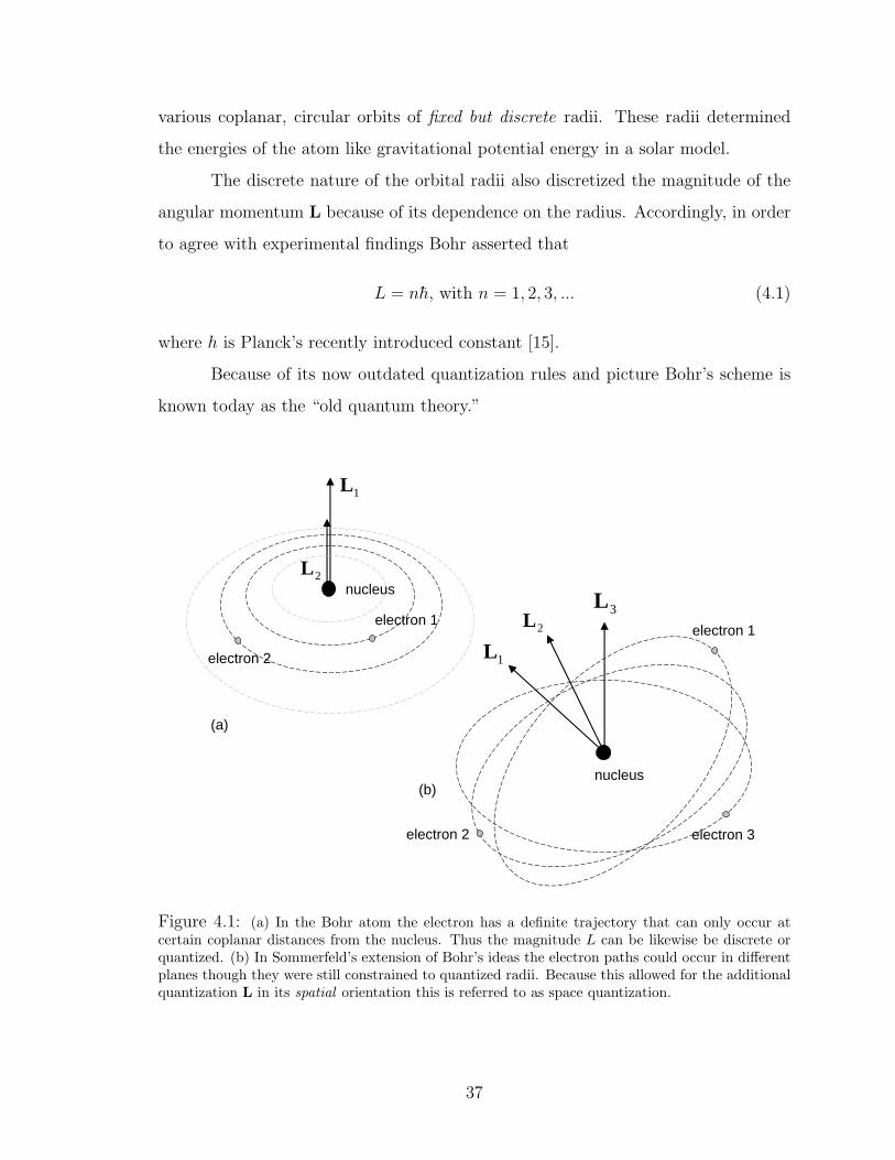
various coplanar, circular orbits of fixed but discrete radii. These radii determined
the energies of the atom like gravitational potential energy in a solar model.
The discrete nature of the orbital radii also discretized the magnitude of the
angular momentum L because of its dependence on the radius. Accordingly, in order
to agree with experimental findings Bohr asserted that
L = nh, with n = 1, 2, 3, ... (4.1)
where h is Planck’s recently introduced constant [15].
Because of its now outdated quantization rules and picture Bohr’s scheme is
known today as the “old quantum theory.”
1L
2L
2L3L
(a)
(b)
nucleus
electron 2
nucleus
electron 1
electron 2
electron 1
electron 3
1L
Figure 4.1: (a) In the Bohr atom the electron has a definite trajectory that can only occur atcertain coplanar distances from the nucleus. Thus the magnitude L can be likewise be discrete orquantized. (b) In Sommerfeld’s extension of Bohr’s ideas the electron paths could occur in differentplanes though they were still constrained to quantized radii. Because this allowed for the additionalquantization L in its spatial orientation this is referred to as space quantization.
37

4.1.2 1916: The Sommerfeld Model
As with any model however the Bohr model of the atom did not fully describe
all the details of observed atomic phenomena. In 1916 Arnold Sommerfeld aided
in extending the Bohr atomic model to other cases including relativistic effects and
the quantization of all three components of L. In doing so the Bohr’s conceptual
representation was altered in a few ways.
The circular coplanar orbits that were visualized in the Bohr atom were re-
placed with orbits that could be distorted to elliptical shapes and could take on
various orientations. They did not have to be coplanar. As a result Bohr’s makeshift
result of a quantized L in magnitude was extended to also include the possibility of
quantizing the direction of L as well.
4.2 1921-1922: Stern and Gerlach’s Experiment
We stop here with the story of atomic models because this is the environment
in which Otto Stern and Walther Gerlach found themselves in 1921. This was the
model - or paradigm - with which they were working.
It was Stern and Gerlach’s intent to verify the Bohr-Sommerfeld model of
the atom by measuring the quantized states of L. As we have seen, based on their
“old” quantum intuition Stern and Gerlach assumed that the atom possessed angular
momentum made manifest in the orbit of the electron about the nucleus. This implied
the presence of a magnetic moment µ which could be manipulated via a magnetic field
B. There were several considerations that would have been either explicitly confronted
or unknowingly passed by. We list a few of these based on what seems appropriate
to us for our purposes.2
4.2.1 Magnet Type
The first consideration may have been of the particular magnetic field con-
figuration that would be used. As we saw in the classical picture of section 3.1 if
2The following may or may not have been exactly how these issues played out in the minds ofStern and Gerlach but only represent how those issues may have been resolved in the given historicalcontext.
38

Stern and Gerlach wanted to observe the magnitude of µ in a particular direction
there were two essential components to the field. They needed (1) a non-uniform
component to B so as to cause the force differential needed to sift the particles by
an observable amount. This amount may have been determined by diffraction con-
siderations, charge, or mass. And (2) Stern and Gerlach needed a preferred direction
to B in order to define the component of µ being measured. In section 3.1 this was
done with the introduction of B0.
Spatial variations of the field had to be considered as well. Once generated
with an appropriate momentum, towards the detector, the particles had to enter and
exit the field. Considered in the frame of the particles this would introduce the same
effects as a time-dependent field. Thus maintaining the desired axial uniformity as
well as avoiding unwanted dynamic effects would have to be considered in order to
make the results clear.
4.2.2 Particle Choice
One way of avoiding several issues with the fringe field effects was to chose
a very specific type of particle. Following Maxwell’s equations this changing B-field
would create an electric field that could exert Lorentz forces on particles carrying
charge. These forces could easily blur the beam in unintended directions disguising
the outcome and interpretation of the experiment.
Stern had worked with beams of silver atoms before so this was the natural
choice. They are electrically neutral but still possess a magnetic moment. That is, in
their neutral state they carry as many protons as electrons but only have one valence
electron so that, while all charge cancels out, there is an “extra” electron orbiting
the nucleus overall thus creating a magnetic moment. These atoms constituted the
beam.
4.2.3 Beam Width
The atoms of the beam were boiled off a filament and accelerated towards
the magnets for measurement. This process imparts a random distribution of both
39
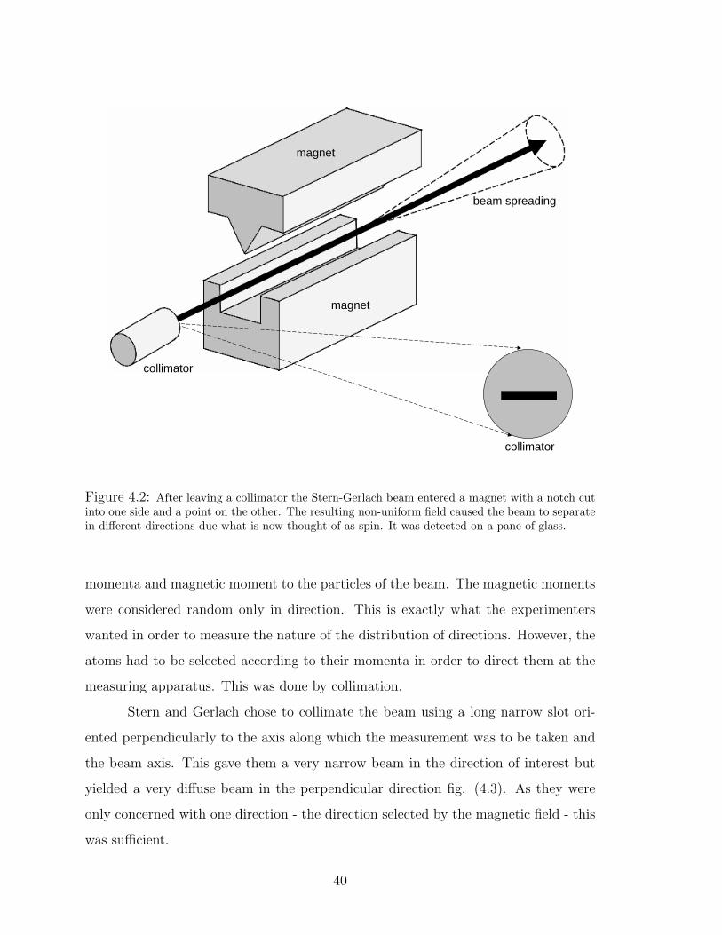
collimator
beam spreading
magnet
magnet
collimator
Figure 4.2: After leaving a collimator the Stern-Gerlach beam entered a magnet with a notch cutinto one side and a point on the other. The resulting non-uniform field caused the beam to separatein different directions due what is now thought of as spin. It was detected on a pane of glass.
momenta and magnetic moment to the particles of the beam. The magnetic moments
were considered random only in direction. This is exactly what the experimenters
wanted in order to measure the nature of the distribution of directions. However, the
atoms had to be selected according to their momenta in order to direct them at the
measuring apparatus. This was done by collimation.
Stern and Gerlach chose to collimate the beam using a long narrow slot ori-
ented perpendicularly to the axis along which the measurement was to be taken and
the beam axis. This gave them a very narrow beam in the direction of interest but
yielded a very diffuse beam in the perpendicular direction fig. (4.3). As they were
only concerned with one direction - the direction selected by the magnetic field - this
was sufficient.
40

(a) (b)
x
z
.03mm
beam into the page (y-direction)
.2mm
Figure 4.3: (a) The cross section of the Stern-Gerlach beam in the y-direction was long and narrowin the xz-plane. (b) The actual images taken from the post card Gerlach sent to Bohr announcinghis results. There is clearly a discrete separation in one direction. Taken from [17].
4.2.4 Results
After sending the beam through the poles of the chosen magnet it proceeded
to a glass plate for detection some distance away where it left a deposition. After
several attempts at fine tuning the apparatus and the intervention of a cheap cigar
[16] a trace was recovered that gave Stern and Gerlach exactly what they had predicted
from theory - a definite separation into two distinct traces oriented along the direction
of the uniform field fig. (4.3).
4.3 1925-1926: Quantum Mechanics
To this point the SGE had been spoken of in terms of mostly classical concepts
and equations. At most it participated only in substantiating the old quantum the-
ory of the Bohr-Sommerfeld atom. The fundamental equations of modern quantum
mechanics had not even been developed yet. It wasn’t until 1925 that Heisenberg
41

developed his matrix formulation for the fundamental characteristics of quantum me-
chanics with his equation
ih∂
∂tA = [A, H] + ih
∂
∂tA (4.2)
in which the arbitrary operator A and the Hamiltonian H are the relevant objects. It
was not until the next year that Schrodinger proposed his more widely recognizable
wave mechanics formulation using the then still mysterious wave function ψ(x).3 His
famous equation
ih∂
∂tΨ = − h2
2m∇2Ψ + VΨ (4.3)
is the time-dependent Schrodinger equation. It is typically found in textbook discus-
sions of quantum mechanics and also used in the previous chapter.
4.4 1925: Spin
The development of these two formalistic systems, the Heisenberg and Schrodinger
pictures, signaled our entrance into a new era of physical science. We were undergoing
a shift of paradigm. With each new unexpected result - and there were many - we
were having to define and redefine the conceptual basis upon which we could build
our theories and against which we would push off when we once again felt equipped
to return to “normal” science.
Once such result that required the introduction of a new concept for its proper
placing in the framework arose from atomic physics. The spectral lines of a given
element could be observed to bifurcate into two closely spaced identical lines when
the element was placed in an extremely strong external magnetic field. This was the
Anomalous Zeeman effect. The word that expressed the concept that was needed to
connect this behavior to others in the quantum framework was coined by two graduate
students, Samuel Goudsmit and George Uhlenbeck, in 1925. It was spin.
It appears that the quantum mechanical concept of spin wasn’t associated
with the SGE of 1922 until 1927.[18]
3Max Born gave ψ its present interpretation as a probability amplitude.
42

4.5 1935: Measurement
During the years under discussion here not only was the scientific community
working out the technical implications of the new quantum regime but they were
simultaneously attempting to define its conceptual foundations. As we have pointed
out, one of the difficult phenomena to translate was that of measurement.
The exact timing of the designation of the SGE as the clearest experimental
demonstration of the measurement problem is not well defined. From a historical
perspective the phenomenon of measurement didn’t force itself into the forefront of
scientific philosophical discussion until 1935 when Einstein, Podolsky, and Rosen pub-
lished a paper challenging the then prevalent byproduct of this quantum conceptual
revolution.4 Their proposal came to be known as the EPR paradox because of its
clear and fundamental repudiation of familiar ideas. It placed the quantum concepts
of entanglement and measurement in the forefront of our framework. Perhaps be-
cause these two concepts are extremely clear and easy to represent in a discussion of
the SGE, as we have shown in the previous chapter, simultaneously with a clearly
distinct classical analogue, the SGE has consequently been given important status as
well. For this reason it is important to address the problems in our descriptions of
the SGE.
4Although the EPR paper was published in 1935 debates and controversy regarding other aspectsof the proper interpretation of quantum mechanics had carried on for as many as 10 years. Thediscussions of the Solvay conference of 1927 are particularly interesting.
43

44
Chapter 5
Problems With Accounts of the Stern-Gerlach Effect
We have given both a thematic, or textbook, account of the SGE and a his-
torical account of the same. The former is built up by the logical ordering necessary
to systematically construct appropriate concepts and the latter by the chronological
ordering of human experience. As representations both presentations emphasize dif-
ferent aspects of the storyline. They also obscure other characteristics either inadver-
tently or because they are explicitly deemed less valuable. In the following we discuss
the assumptions and inconsistencies that are hidden in the two previous accounts
but that are rashly dismissed either because of tradition, practicality, or misunder-
standing. Before considering the limitations of these two accounts however we will
consider some limitations that appear to apply more generally to quantum mechanics,
and even science, as a whole.
5.1 Problems from Quantum Mechanics
In section 2.3.3 we introduced wave-particle duality as an example of orthogo-
nal concepts. We called such concepts “orthogonal” because, like orthogonal vectors
or functions, the concepts implied by one cannot in any way be represented in terms
of the concepts implied by the other. In the language of logic the two are mutually
exclusive. In this sense orthogonal concepts are also describable in terms of Bohr’s
principle of complementarity in which two disparate concepts are required in order
to fully describe a single phenomenon (see discussion in section 2.2).
45

5.1.1 Rightness and Clarity
Among the many of concepts that serve as effective conceptual basis sets for
describing any scientific concept are the concepts of rightness and clarity. They are
an effective basis because they are “orthogonal” or complementary. As applied to
Some Orthogonal Concepts
Rightness ClarityWaves Particles
Position MomentumJustice Mercy
Creativity ConformityHumility ConfidencePatience Ambition
Form FunctionConstancy Change
x y
Table 5.1: A listing of some orthogonal concepts to which Bohr applied his principle of comple-mentarity. Just as with coordinate axes it is precisely because of their orthogonality that they areuseful in describing other, more complicated, ideas. [19]
representations we can see that the more effort that is put into making a presentation
simple, clear, and accessible the more idealization, approximation, and artificiality
are in it. Whereas if a strenuous effort is made to represent all the facts in their
proper context so much complication and technicality are introduced that a useful
understanding of them becomes near impossible. In short, the more clear a represen-
tation is made to be the less right it is whereas the more right it is the less clear it
can be. Thus there is a fundamental tension between the rightness and clarity of a
statement.
46

5.1.2 Representations as a Map
This can be demonstrated by considering a map. Maps are representations
of regions of space. The more detailed the map the bigger and bulkier must be its
pages with expanded scaling and legends whereas the more compact and simple the
map the less detail can be described by it. To maximize its correspondence to reality
at the expense of user-friendliness would make the map no different than the terrain
it describes while increasing its immediate and efficient use would surely omit some
detail that could become important.
5.1.3 Communication
The simultaneous maximization of both the clarity and rightness of a state-
ment is the aim of effective representation and communication. However, in quantum
mechanics this discrepancy between what is and what we understand is manifest in
even stronger terms than in other fields. It was a common opinion among the archi-
tects of quantum theory that although quantum phenomena were incompatible with
classical concepts, due to the classical nature of the equipment, i.e. its compatibility
with humans on the macro-scale, only these concepts could be used to describe them.
For example, Bohr [20] has said that
In this context, we must recognize above all that, even when the phe-
nomena transcend the scope of classical physical theories, the account of
the experimental arrangement and the recording of observations must be
given in plain language. (p. 72)
and Heisenberg [21] has written that
Any experiment in physics, whether it refers to the phenomena of daily
life or atomic events, is to be described in the terms of classical physics.
(p. ??)
In other words, the common opinion is that although nature fundamentally behaves
quantum mechanically humans can only understand it in terms of classical concepts
47

because we can only interact with this level.1 Unfortunately for us, classical concepts
are also inadequate.
Thus, it is a frustrating axiom of modern paradigm that clear communication
is exactly opposed to correct communication. As one aspect is refined or improved the
other is helplessly compromised. This may be suggestively expressed in the schematic
form
∆Clear∆Right ≥ constant, (5.1)
reminiscent of eq. (3.31).
When students find this out for themselves it is not unlike entering hell in the
Divine Comedy.2
5.2 Problems with Historical Accounts
In terms of understanding the SGE some historical details might be missed
- either deliberately or ignorantly - in the historical accounts but of more concern
for us here is their lack of clarity. Consequently we will not spend time here to
discuss the problems of historical accounts as regards to facts but only emphasize
their pedagogical limitations.
There are some of the concerns common to these sorts of accounts.
More historical detail, whether of science’s present or of its past, or
more responsibility to the historical details that are presented, could only
give artificial status to human idiosyncrasy, error, and confusion. Why
dignify what science’s best and most persistent efforts have made possible
to discard? [2]
Indeed, including all the facts associated with each “dead end” pursued by each
researcher is impractical and surely confusing to students at an introductory level.
At this point students need a clear, linear progression that builds the concepts in a
logical way so as to make them as graspable as possible. Unfortunately this is not
1For a similar discussion see also [22] p. 127-130.2In Dante’s classic The Divine Comedy the inscription above the doorway leading to hell read
“Abandon hope, all ye who enter here.”
48

how history typically unfolds. The development of science is often more messy than it
is linear - running into several problems followed by some backtracking before making
a small but successful advance. Sometimes paths are vigorously pursued only to show
they are fruitless.3 Thus, in the attempt to make the story of the SGE correspond to
the reality of the events, which for some purposes is a worthy goal, for instructional
purposes clarity is lost.
5.3 Problems with Thematic Accounts
On the other hand, the strength of thematic accounts of scientific events is
precisely their clarity. However, according to the dual relationship hinted at in eq.
(5.1) this implies only a crude correspondence to fact or reality. As the bulk of this
work will assess the accuracy of thematic accounts with a special emphasis on their
technical aspects (see the next chapter, in particular) we will spend the remainder of
this chapter developing these ideas.
5.3.1 An Artificial History
First, in a general sense opposite to that of section 5.2 the thematic accounts of
textbook or classroom discussions are very linear and cumulative in their presentation
and use of concepts. That is, before a particular concept is needed in the descrip-
tion of an event that concept is either motivated or derived from previous concepts.
This of course removes concepts out of their historical context and therefore assigns
them an artificial and unscientifically acquired meaning. This also necessitates the
eventual acceptance of certain axioms which ultimately have no justification but are
deemed useful.4 However, convenience is too often confused with correctness. These
considerations lead us to the conclusion that there is little that corresponds to reality
in these accounts. Their final justification is only that they are clear and that they
3The word “fruitless” here is a misleading word. While such a path may be “fruitless” as regardingthe desired result, inasmuch as an understanding of what definitely will not work is gained this is avital step forward in producing progress.
4For this reason [2] tells us that it is the purpose of textbooks to communicate paradigms andnot to communicate facts.
49

posses an accurate predictive power. This says little, however, about the accuracy of
the conceptual structure that had to be built up.
From contrasting the thematic account in Chapter 3 with the historical one
of the Chapter 4 we can surmise that there are several misconceptions that students
could have after having been taught the SGE.
(1) The original SGE was observed several years prior to the development of
the quantum theory and spin. Hence, although it is often used as a confirmation or
demonstration of modern quantum concepts such as spin and measurement it was in
no way motivated by or intended for this purpose.
(2) The observation of the SGE actually confirmed the historically prevalent
theory of the time - the Bohr-Sommerfeld model of the atom - which is now consid-
ered false.5 It did not surprise the experimenters for this is exactly what Stern had
predicted previously [23]. Those doors had either already been open, such as with the
Bohr model’s quantization, or would not be open for years, such as the incorporation
of spin into the quantum framework. Therefore, the SGE did not signal the opening
of a new door in physics or philosophy but the relatively unexciting continuance of
the present paradigm.
(3) It is interesting to note that the SGE clearly demonstrates how the right
results6 - even experimental results - can be used to justify an erroneous account of the
phenomena and then also be given canonical and defining status in a completely new
conceptual system. This demonstrates the subjectivity of representations in science
well.7
[2] describes some of the general deficiencies of thematic approaches as well.
It says,
The result [of the thematic approach of textbooks] is a persistent ten-
dency to make the history of science look linear or cumulative... The
5On a post card communicating the results of their experiment to Bohr Gerlach writes “Wecongratulate [you] on the confirmation of your theory.” See [17]
6This is clumsy language. Results can never be wrong especially in experimental physics; onlyour questions or our interpretations of the results can be difficult.
7This is similar to the researcher who can always seem to get the answer he’s looking for preciselybecause he’s looking so hard for it.
50

textbook tendency to make the development of science linear hides a pro-
cess that lies at the heart of the most significant episodes of scientific
development. (p. 137-140)
It hides the true nature of the most interesting research questions.
5.3.2 Misunderstanding the Practical Aspects of the Stern-Gerlach Effect
Related to misconceptions as to the historical ordering and significance of
events are the practical experimental considerations which we included in sections
4.2.1-4.2.3. They concern (1) the species of particle in the beam, (2) selection of
beam cross section, and (3) the type of magnetic field used.
The usual de-emphasis of these three points in thematic accounts of the SGE
has some interesting consequences.
(1) (See section 4.2.1) Because all the talk of the SGE is couched in terms of
spin-1/2 particles the idea, if not the word explicitly, of the electron is used. It is
considered the canonical spin-1/2 particle. However, this practice hides a whole field
of very interesting research. Students don’t realize that there is a time-dependence to
the magnetic field due to its approaching speed relative to the particle which exerts a
transverse Lorentz force on it. Because this phenomenon is dependent on the presence
of charge the SGE has never been observed with electrons. In fact, Bohr and Pauli,
among others were of the opinion that the electron SGE could never be observed [24].
This points out an inconsistency. As a canonical example of spin-1/2 particles
electrons should display the SGE as do other spin-1/2 particles like silver.
Despite this, there is much research going on to overcome these blurring effects
with fruitful results. Because this whole field opens more questions than it answers,
which compromises clarity, it is often neglected.
(2) (See section 4.2.2) The astute reader might find an inconsistency between
what is said and what is shown. Typically when the idealized SGE is discussed in
textbooks it is spoken of in terms of a point-like beam for reasons of clarity. When the
original trace of the experiment is also shown as in fig. 4.3 this is inconsistent. If both
of these are taken as accurate then it seems there was a continuous blurring in the
51

horizontal direction that accompanied the discrete separation in the field direction.
If this is not pointed out it can be confusing whereas if it is it incorporates many
unnecessary experimental details that make its description bulky and difficult.
The previous point is especially important when considering the SGE as a
demonstration of quantum measurement because it is accepted that the entire exper-
imental context defines the phenomenon. In other words, if this is not made clear
then it is unclear as to what we are really measuring. Students may be left wondering
if a point-like SGE ever been attempted and if not, why not? This is difficult to
determine from thematic accounts because so little is ever said about the specifics of
the collimation.
(3) (See section 4.2.3) As a discussion of the misconceptions regarding the
specifics of the magnetic field introduces the more technical aspects of thematic ac-
counts and has lead to numerous questions it is treated in its own section.
5.4 The Magnetic Field
As was argued in section 3.1 the magnetic field
B = (B0 + bz)z (5.2)
is the simplest field to meet the physical requirements of the question that Stern and
Gerlach sought to answer. In fact, this is a typical representation of the field as given
in many discussions of the SGE. It is rarely mentioned however, especially in explicit
terms, that there is at least one other physical constraint on the field.
Maxwell’s equations for all electromagnetic fields specify that B must satisfy
∇ ·B = 0 (5.3)
∇×B = µ0J +1
c2∂
∂tE (5.4)
where E is the electric field and c is the speed of light in vacuum. µ0 is the magnetic
permittivity of vacuum. Because of eq. (5.3) B must be inhomogeneous in at least
two directions
∇ ·B =∂
∂xBx +
∂
∂yBy +
∂
∂zBz = 0. (5.5)
52

So a better choice would be
B = −bxx+ (B0 + bz)z (5.6)
because∂
∂xBx = − ∂
∂zBz. (5.7)
As a fortunate consequence ∇ × B = 0 so in accordance with eq. (5.4) there are
no dynamically changing fields. This is the simplest magnetic field that satisfies the
conditions of Stern and Gerlach’s question - it has homogeneous and inhomogeneous
parts - as well as Maxwell’s physical constraints. For reasons of clarity the field is
often not treated this way. This is however the difference between a description of the
SGE that is consistent with the fundamental equations of electricity and magnetism.
and one that is unphysical.
It should also be pointed out that there are other constraints to further define
the field. One that may prove important later is the physical requirement that the
field remain finite at all distances. As it is now, the field linearly blows up with
increasing distances away from the origin. That is,
limr→∞
B = ∞ (5.8)
where r =√x2 + z2. To get around this we can either append the field with an
exponential factor that enforces the required asymptotic fall off or merely truncate
our range of interest to a finite region. The second of these is more artificial than the
first. These considerations will be taken up in more detail in section 6.1.1.
5.5 Precession Arguments
Notwithstanding the inaccuracies in the field of eq. (5.2), as we have shown,
it can still yield correct results. This indicates that there must be some physical
justification for neglecting it. When the necessary complication of the full field is
used it is the phenomenon of precession that is said to justify the neglect of the
transverse inhomogeneity. We will consider how this is done in both the classical and
quantum regimes.
53

5.5.1 Classical Precession
We have shown in section 3.1 and it has been more rigourously demonstrated
in [25] and [26] that the presence of the homogeneous field component B0 causes a
precession of the classical vector µ. From the torque equation
d
dtµ = ω × µ (5.9)
given there µ can be found and substituted into the force equations. [25] and [26] show
how when the time average of the force is calculated only the force in the z-direction
turns out to be non-zero. From this fact it is argued the inclusion of precession in the
right way justifies the neglect of all x-oriented dynamics.
It is interesting to consider what the “right way” consists of. Even in this clas-
sical picture the approximations are crude. As [26] explicitly points out the required
relation is not just that there is a homogeneous component to the field but that
|Bhomogeneous| >> |Binhomogeneous| (5.10)
or, in the case of eq. (5.6)
|B0| >> |br| (5.11)
where r =√x2 + z2. What is more subtle is that [26] then applies this particular
criterion with the approximation that
B ≈ B0z. (5.12)
In other words, this inequality eq. (5.11) is only useful if it justifies the complete
neglect of the inhomogeneity. So, in the classical treatment of [25] and [26], the field
necessary to induce adequate precession, i.e. a strong uniform field, is exactly the
field that prohibits the separation of spins by a net force, i.e. an inhomogeneous part.
This is crude at best and inconsistent at worst.
There is one further condition on the experimental set up that is required for
practitioners of classical physics to invoke the precession argument. Conditions must
be chosen such that the time of interaction, or the time it takes the particle to pass
through the region of space in which the field is significant, must be much greater
54

(b) nT
(a)
3T
(n=3)
Figure 5.1: (a) If the time of interaction nT is roughly equivalent to or less than the period Tof the precession frequency, that is n ≤ 1, then the net area between the precessing curve and theaxis is large. (b) If n � 1 such that several precession cycles occur during the time of interactionnT then the portion of the shaded region that does not cancel out is much smaller. In other words,for the same nT the total shaded region for a slowly precessing spin is much larger than that fora rapidly precessing spin. Inasmuch as the shaded region corresponds to the accumulated affect ofthe transverse force in time, i.e. its time-average, the transverse deflection of the beam only washesout in (b). For (a) we would still expect a transverse deflection.
than the period of precession. This allows the x-directed forces to adequately “wash
out.” Without this the average x-force would tend to favor one side or the other.
5.5.2 Quantum Precession
In thematic accounts in which the quantum version of the precession argument
is used to justify the use of a non-Maxwellian field configuration it is the expectation
value of the spin that precesses and not the spin itself. This is an extremely subtle
point.
Note that in the present context we use “spin” S instead of “magnetic mo-
ment” µ according to their relation
µ =ge
2mS. (5.13)
Recall also that
S =h
2σ (5.14)
55

where
σx =
0 1
1 0
, σy =
0 −i
i 0
, and σz =
1 0
0 −1
(5.15)
as before.
Precessing Expectation Values
In order to show this we place a particle with spin 1/2 in a uniform B-field in
the z-direction
B = B0z. (5.16)
Using this in the Hamiltonian
H = −µ · B (5.17)
we can find the general states and energies as in section 3.2.1
Ψ = ψ↑χ↑e−iE↑t/h + ψ↓χ↓e
−iE↓t/h. (5.18)
With these states, the expectation value of S, or more specifically 〈Sx〉, 〈Sy〉,
and 〈Sz〉, can be evaluated. First we write
〈Ψ|Sj|Ψ〉 (5.19)
where
Ψ = ψ↑χ ↑ e−iE↑t/h + ψ↓χ↓eiE↓t/h. (5.20)
So, if j = x
〈Sx〉 = 〈Ψ|Sx|Ψ〉 =h
2
(ψ∗↑ψ↓e
ih(E↓−E↑)t + ψ∗↓ψ↑e
ih(E↑−E↓)t
). (5.21)
Note that all the time-dependence is carried by factors that depend on the difference
of the energy of the two states, more specifically (E↓ − E↑) and (E↑ − E↓).
Applying this procedure to Sy and Sz as well we get
〈Sx〉 =h
2sin θ0 cos
(eb
mt
)(5.22)
〈Sy〉 =h
2sin θ0 cos
(eb
mt
)(5.23)
〈Sz〉 =h
2cos θ0 (5.24)
56

where θ0 is the angle the spin vector makes with the z-axis. Thus, as time progresses
〈Sz〉 is constant and 〈S〉 = 〈Sx〉x+ 〈Sy〉y rotates, or precesses, in the xy-plane.
To clearly see the effect of this precession on quantum expectation values
we take the time average. In general if we wanted to find the time average of some
oscillating function f(t) where the frequency of oscillation is ω = 2π/T over n periods
T . We would evaluate
f(t)avg =1
nT
∫ nT
0
f(t)dt (5.25)
Applying this averaging formula to the expectation values above we see that
〈Sx〉avg = 0 (5.26)
〈Sy〉avg = 0 (5.27)
〈Sz〉avg =h
2. (5.28)
Thus, over significant time intervals the expectation values 〈Sx〉 and 〈Sy〉 “wash out,”
or go to zero, whereas 〈Sz〉 is constant.
Problems with Precession
In the standard description of the SGE this “washing out” effect of the expec-
tation values is referred to in order to justify the neglect of the transverse inhomo-
geneity of eq. (5.6) and the use of a divergenceless field eq. (5.2). Some merely cite
the classical case of the phenomenon as justification [27] while some refer to the fully
quantum demonstration given above [1], [9]. Even in the latter case however, when
the demonstration is explicit, this is inconsistent for at least three reasons.
(1) The above derivation depended critically on the value of the energies or,
more specifically on the difference of the energies. Therefore, in order to rigorously
justify the neglect a certain component of the spin we had to have already solved for
the energies which already would have involved that spin component, i.e. using eq.
(5.25) with eq. (5.21) as the integrand. Although intuitively easy this is logically
invalid and probably glosses over interesting questions.
(2) The precessing solutions found in the homogeneous field of eq. (5.16) were
rigourously obtained but then subjectively applied to a completely different problem
57

- one involving the field of eq. (5.6). This assumes that the interaction of these
phenomena - the uniform and non-uniform parts of the field - is linear and can be
naively superposed. However, it will be seen in Chapter 7 that solving only the non-
uniform part is not trivial. This suggests that more than just a linear interaction is
occurring.
(3) Finally, just because the expectation value time-averages to zero doesn’t
mean the measured value is zero or even that it is close to zero! According the the
interpretation discussed in section 3.2.2 this only means that the average of several
measurements all preformed on identical systems will be zero but any one could be
arbitrarily large. This says nothing about one measurement in particular.8
From all these considerations it is obvious that at best the precession argu-
ment that is traditionally invoked in thematic accounts of the SGE disguises several
interesting questions and at worst is completely invalid and inaccurate.
5.5.3 Precession and the Uncertainty Principle
If there is a possibility that the precession argument is misapplied in the stan-
dard interpretation of the SGE then there is also a possibility of other misinterpreta-
tions as well. One of these has to do with the uncertainty principle.
We saw in section 3.2.4 that for any two non-commuting operators A and B
such that
[A, B] = AB − BA = C (5.29)
in the quantum formalism there is a corresponding uncertainty relationship
∆A∆B ≥ |〈C〉|2
(5.30)
which is typically interpreted as a constraint on the physical process of measurement.
That is, as A is measured to a given degree of precision the quantum state of the
system being measured is altered in such a way as to limit the precision with which
B can be simultaneously measured.
8Exactly how much it says about a collection of many measurement is dictated by eq. (3.30).
58

Because the three components of the spin operator S do not mutually commute
they satisfy an uncertainty relationship as well
∆Si∆Sj ≥ iεijkSk. (5.31)
We interpret this to mean that we cannot simultaneously measure two components
of the spin to an arbitrary degree of accuracy. It is precisely the phenomenon of
precession that allows this interpretation.
If for some reason precession could not be invoked as a valid occurrence then
in the SGE our classical intuition would lead us to believe that the particle would
arrive at the detection screen purely due to spin forces. If the particle were found
at a 45◦ angle from the location of the localized y-directed beam in the field then
we would assume the particle felt an equal force in both the x and z-directions. The
formalism tells us that these forces, and thus deflections, arise in proportion to the spin
component in the corresponding direction. Therefore, we would classically interpret
such a result as a simultaneous measurement of both the x and z-components of the
magnetic moment.
In a quantum context the same arguments apply but with more at stake. It
is the relative strength of one direction to the other that justifies the presence of
precession and it is this precession that gives the “washing out,” or ambiguity, of
the transverse spin components necessary to the interpretation of the SGE in terms
of the uncertainty principle. From this it seems that if the preferred direction were
removed for the Stern-Gerlach measurement of a single particle, precession would also
be removed and there would be nothing to rescue us from simultaneously measuring,
or assigning definite values to, two orthogonal spin components of a single particle.
Thus, it is possible that our present understanding of the uncertainty principle only
follows from our choice of field and not from the nature of the particles themselves.
We accordingly will use the problems outlined here as a motivation and guide
to the work and questions of the next chapter. In addition to the broad problems
outlined so far there are many more smaller and more specific problems that arise
in discussions of the SGE. These will be brought up in the appropriate places in the
59

next chapter as we investigate the nature of the SGE in several contexts and in more
depth. This offers us several interesting possibilities for not only gaining a deeper
understanding of the SGE but, more generally, of our interpretations of physics.
60

Chapter 6
The Proposal
The SGE is widely thought to have a description that is not only conceptually
very clean with relatively few mathematical technicalities but that clearly demon-
strates some fundamental characteristics of quantum behavior. Yet despite its clear
break from classical expectations as we saw in the previous chapter our justifications
for the SGE description have yet to break free of classical traditions. Consequently,
there are few, if any, fully quantum descriptions that do not make reference to out-
dated notions.1
As an example of this, we see that in order to motivate the use of a magnetic
field which clearly violates Maxwell’s equations many authors cite and/or derive the
classical phenomenon of precession. This causes an averaging away of spin compo-
nents transverse to the magnetic field so that the transverse behavior can be ignored
from the beginning. However, as we saw in section 5.5 this is an ad hoc assumption
and has not been shown to easily follow from rigorous solutions. We are therefore
unaware of its implications. In addition, while this approach may be sufficient clas-
sically when applied to quantum mechanical descriptions of nature only expectation
values can be expected to precess. Invoking this argument then in reference to the
SGE blurs the distinction between classical and quantum conceptual systems which,
because of their stark differences and the necessity of clear and consist conceptual
representations for rational communication (see section 2.1), leads to further confu-
sion. If the quantum formalism is complete it should provide us with an appropriate
1[28] and [29] make reference to this same thought so work in this area is mounting.
61
basis for describing the SGE.2 Not only will this demonstrate consistency but it will
allow us to uncover questions that have previously remained unasked merely because
of self-enforced conceptual boundaries.
6.1 Positivist and Realist Representations
The formulation of a specific question that attempts to reveal the true nature
and applicability of the SGE with its precession arguments can be motivated by
contrasting two opposing conceptual, or representational, systems. We will call these
the orthodox and realist views [1], [8].
The positivist position, which most closely resembles the orthodox or main-
stream position, has become known as the Copenhagen interpretation. It states that
prior to a measurement of a particular quantum property that property did not have
a well defined value. It is the act of measurement that compels the particle to assume
a definite value. In terms of a spin measurement via a Stern-Gerlach apparatus spin
is not considered definite, i.e. it is not considered to take on one orientation or one
magnitude, until the particle strikes the detection plate.3 Prior to this the most that
can be said of the particle’s “spin” is that it was in a superposition of spin “up” and
“down” states. In terms of position the particle was in a superposition of deflecting
“up” and deflecting “down”.
In the realist opinion, these properties exist independent of the measurement
process but are affected in complicated ways by it. In other words, the existence of
these properties is independent but their specific value is not.4 As applied to spin,
there is always a spin property to a particle, perhaps even zero, though its particular
2Because we have spoken of the SGE as an axiom of modern physics there could be an interestingdiscussion here on the applicability of Godel’s Incompleteness Theorem.
3This statement emphasizes clarity at the expense of rightness. Exactly when measurement occursis an open question contributing to the quantum problem of measurement summarized in section3.2.3. Does it occur upon collision of particle with plate, with the gaze of a conscious observer, orsomewhere in between (see [11] and [12])? In an ironic twist of quantum fate because we cannotmeasure measurement it seems we will never quite have a definite answer.
4The specific identification of the content of the realist and positivist positions is difficult becausethere is so little consensus as to particulars. We should point out that there are intermediary positionsin which existence is still independent of measurement but completely unknowable due to the effectsof the measurement process. Philosophically this might correspond to Kant’s discussion of noumenaand phenomena. As stated here realism sounds very Randian. See [4].
62
orientation and magnitude are changed in ways that are heavily dependent upon the
entire experimental arrangement, i.e. the distance to the screen, the orientation of
the field, etc. [12]
Because in the positivist view the spin is not said to be an element of reality
until measurement occurs it seems inconsistent to invoke the precession argument to
justify the neglect of part of the field. Its neglect must be attributed to something
other than the property of spin. The realist has no such problem. In this sense, this
could serve as a crucial experiment for very particular views of realism and positivism.
6.1.1 The Changing Role of Precession
Because developing a deeper understanding of the SGE depends critically on
the precession argument we must ascertain the true effect of precession, its validity,
and its range of applicability. This can be done by considering its interaction with the
spin or magnetic moment and its dependence on the homogeneous field component.
Is there any reason to apply this homogeneous field component? Its only
purpose classically seems to be to induce precession about the direction of interest so
that only that components in that direction will be clearly observed. As mentioned in
section 5.5.3 the question becomes more interesting when we consider its implications
in the quantum picture.
Although it seems it was introduced historically only to label the direction
of interest it seems it has been preserved through the quantum revolution because
our conceptual picture, the prevailing positivist view, requires it. Put differently,
whereas in the old paradigm it was justified by our desire to measure only a single
component of the magnetic moment, it has now become the justification for our belief
that measuring only one component is possible, via the uncertainty principle.
This demonstrates the little noticed effect of paradigm on experimental prac-
tice. [2] explains that
consciously or not, the decision to employ a particular piece of ap-
paratus and to use it in a particular way [as with the homogeneous field
63

component] carries an assumption that only certain sorts of circumstances
will arise. (p. 59)
In addition to the usual theoretical expectations these instrumental expectations
“have often played a decisive role in scientific development.”
6.2 Proposal: The Inhomogeneous Stern-Gerlach Effect
The most direct way that we propose to discover the true nature and effect of
the precession argument on not only the measurement of spin but on our theoretical
description and general interpretation of measurement as well is to theoretically re-
move the homogeneous field component which is the element that selects a universally
preferred direction and which is the precession inducing agent. More explicitly, we
propose to solve the SGE with a beam travelling in the y-direction by replacing the
typically studied field configuration
B = (B0 + bz)z (6.1)
with the its more natural choice
B = −bxx+ (B0 + bz)z. (6.2)
We have included the constant component B0 only so that the phenomenon of pre-
cession can be explicitly shown as opposed to its usual imposition. We can either set
B0 = 0 in order to solve the inhomogeneous SGE (ISGE) or leave it as a non-zero
constant to test the known Stern-Gerlach limit.
Note that either choice is physically consistent with the requirement that
∇ ·B = 0. (6.3)
The field does however blow up linearly far away from the origin.
6.2.1 The Experimental Arrangement
If we consider the physical realization of this field we can perhaps avoid this
difficulty. The field eq. (6.1) may be considered an approximation to a configuration
64
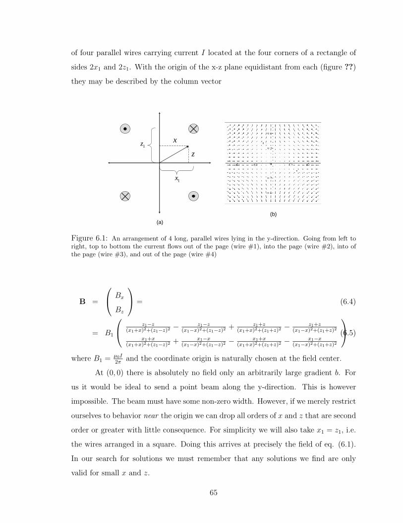
of four parallel wires carrying current I located at the four corners of a rectangle of
sides 2x1 and 2z1. With the origin of the x-z plane equidistant from each (figure ??)
they may be described by the column vector
1x
1zx
z
(a)(b)
Figure 6.1: An arrangement of 4 long, parallel wires lying in the y-direction. Going from left toright, top to bottom the current flows out of the page (wire #1), into the page (wire #2), into ofthe page (wire #3), and out of the page (wire #4)
B =
Bx
Bz
= (6.4)
= B1
z1−z(x1+x)2+(z1−z)2
− z1−z(x1−x)2+(z1−z)2
+ z1+z(x1+x)2+(z1+z)2
− z1+z(x1−x)2+(z1+z)2
x1+x(x1+x)2+(z1−z)2
+ x1−x(x1−x)2+(z1−z)2
− x1+x(x1+x)2+(z1+z)2
− x1−x(x1−x)2+(z1+z)2
(6.5)
where B1 = µ0I2π
and the coordinate origin is naturally chosen at the field center.
At (0, 0) there is absolutely no field only an arbitrarily large gradient b. For
us it would be ideal to send a point beam along the y-direction. This is however
impossible. The beam must have some non-zero width. However, if we merely restrict
ourselves to behavior near the origin we can drop all orders of x and z that are second
order or greater with little consequence. For simplicity we will also take x1 = z1, i.e.
the wires arranged in a square. Doing this arrives at precisely the field of eq. (6.1).
In our search for solutions we must remember that any solutions we find are only
valid for small x and z.
65

We can also give a form for the vector potential that satisfies this approximate
field. It is
A = B0xzy. (6.6)
However, even including minimal coupling as we have our choice to use only neutral
particles will make the vector potential unimportant.
Sending a beam of neutral spin-1/2 particles, i.e. neutral silver atoms, along
the y-axis in such a field will exhibit the ISGE.
(a) (b) (c) (d)
Figure 6.2: (a) The beam splits in both x and z-directions. (b) The beam splits in the radialdirection only. (c) The beam splits into two angular direction. (d) The beam does not split butblurs in all directions. Some blurring will arise from collimation so in this case it would be importantto note whether the observed blurring was attributable to spin separations.
6.2.2 Possible Outcomes
In the case that the B0 = 0 choice is made what beam trace can we expect?
Fig. 6.2 shows four possibilities. If we choose the experimental conditions, i.e. the
time of interaction nT and the strength of the field gradient b, so as to invalidate
precession arguments any result would be instructive. Moreover, because of the ab-
sence of precession, if it is run for only a single particle its deflection and detection
anywhere on the plate would naively define 2-components of the “force” or, conse-
quently, 2-components of the spin. For reasons discussed in section 5.5.3 this is of
extreme interest.
66

Chapter 7
A More Complete Study of the Stern-Gerlach Effect
In accordance with the proposal of the previous chapter we seek here to find
solutions and insights into the Inhomogeneous Stern-Gerlach Effect (ISGE). Because
of the difficulty and nature of the task we will represent this problem in using several
solution methods, formalisms, and pictures in an attempt to fully understand this
effect in a quantum context along with its theoretical and philosophical implications.
7.1 Matrix Representation in a Moving Frame
In order to gain an initial familiarity with the full SGE, and in particular the
ISGE, we can follow the method used in Chapter 3 only with the slightly modified
field eq. (5.6). We begin with a Hamiltonian operator describing the ideally impulsive
interaction of duration T as
H(t) =
0 for t < 0
− em
h2
(B0 + bz) −bx
−bx −(B0 + bz)
for 0 ≤ t ≤ T
0 for t > T
. (7.1)
7.1.1 The Assumptions
This is a special representation of the Stern-Gerlach Hamiltonian. As was
stated, but not discussed, in Chapter 3 this considers the dynamics from the frame of
the particles in the beam which we take to be inertial. As this assigns the definite value
of zero to px and pz it correspondingly limits the possible definition of the position
67
according to eq. (3.31). The incoming beam is therefore a plane wave travelling in
the y-direction with infinite extent in the x and z-directions. As it was shown in
Chapter 3 the y-behavior can be separated off without any assumption on py.
For completeness we should also consider the effects of the idealization involv-
ing the impulsive field. In reality no field can be turned on infinitely quick or confined
perfectly to a given region of space without some variation. In our case, in the rest
frame of the beam particles, this would be manifest as a time-varying B-field, which
via Maxwell’s equations sources electric fields. This could cause some complicated
effects as the particle enters and exits the field. However, a numerical treatment
of the ISGE involving charged particles using a field with a non-zero “turn-on” and
“turn-off” time showed no significant differences from the idealized case [30]. Because
of this and because we have chosen to work only with neutral particles we think that
the idealization of an impulsive field is adequate.
7.1.2 The Eigenstates
The energies can be found in the same manner as in section 3.2.5 with a similar
result. We get
E↑↓ = ∓ eh
2m
√(bx)2 + (bz +B0)2. (7.2)
where the ↑↓ refer two possibly resultant states as represented in the z-basis. We
should also point out the apparent spatial dependence of the energies. This was also
present in the treatment in Chapter 3. In order to make sense out of these spatially
dependent eigenvalues the factors of x and z in eq. (7.2) should be thought of as
parameters and not as spatial coordinates. If the beam were localized enough they
might refer to the coordinates of the peak of the beam packet in the xz-plane. But for
a beam that is extended compared to the region of interest as we have, (x, z) could
be thought of as the initial position of the particles within the beam as in a realist, or
pilot-wave-type visualization (See section 7.12.1 for further discussion). Either way,
they should be thought of as parameters and not variables.
68
Although we will not need them we point out that the eigenvalues eq. (7.2)
correspond respectively to the non-normalized eigenstates
| ↑↓〉 =
1
− p2↑↓
ehbx+ B0
bx+ z
x
(7.3)
with p↑↓ = 2mE↑↓.
For t < 0 the field is off so we have a free particle at rest since H = 0 (E = 0).
At t = 0 the field is switched on and as we found earlier the states are describable as
Ψ = ψ↑χ↑ei e2m
√(bx)2+(bz+B0)2t + ψ↓χ↓e
−i e2m
√(bx)2+(bz+B0)2t. (7.4)
This persists until t = T after which time the particle is again unaffected so the final
states can be found by merely evaluating eq. (7.4) at t = T .
7.1.3 Demonstrating Precession
If we take the limit that ε is small where ε = b/B0 such that |B0| >> |br| for
all relevant values of r =√x2 + z2 we can demonstrate the effect of the precession
argument but without reference to the classical or quantum concept of precession.
If we expand the squares in the phase ϑ of eq. (7.4) we can write
ϑ = ±i e2m
√B2
0 + 2B0bz + b2r2t. (7.5)
Since we take B0 to be large let us factor it out of the radical
ϑ = ±ieB0
2m
√1 +
2bz
B0
+
(br
B0
)2
t (7.6)
Expanding the radical for small ε we get
√1 + 2εz + ε2r2 = 1 + εz +
ε2
2x2 + ... (7.7)
So to first order the phase is
ϑ = ±i e2m
(B0 + bz)t (7.8)
which is exactly the phase of the solutions we found in Chapter 3 (see eq. (3.36)). This
is a purely mathematical demonstration, within a few assumptions, of what is hap-
pening in the standard derivations of the SGE. It shows that despite the logical and
69

mathematical heuristics that often go into making a thematic discussion of the SGE
intuitive there is a more mathematical and clearly demonstrable reason the physical
picture works. Whether precession accounts for this is a matter of interpretation.
7.1.4 The Inhomogeneous Stern-Gerlach Effect
Now that we can clearly see that B0 justifies the precession picture and the
neglect of the x-directed field we can let B0 → 0 to solve the ISGE. This should clarify
the role of precession even further.
t
rp+
(a)
(b)
spin “up”moves “out”spin “up”
moves “out”
rp−spin “down”
moves inspin “down”
moves in
Figure 7.1: As time progresses the spins separate radially “up” or “down” depending on their spinorientation relative to the radial direction.
Returning to eq. (7.4) but with B0 = 0 we can write the final inhomogeneous
Stern-Gerlach states
Ψ = ψ↑χ↑eih( ebTh
2m)r + ψ↓χ↓e
− ih( ebTh
2m)r. (7.9)
70

Using the same arguments as in section 3.2.5 we may interpret this as two circular
plane waves travelling either radially outward or inward with a momentum
pr = ±ebT h2m
(7.10)
depending on its spin’s projection along the z-axis. Relative to this axis the spin
“ups” move radially outward while the spin “downs” move towards and through the
center of the field.
7.2 Position and Momentum Representations
We can now attempt a more rigorous solution that involves fewer assumptions
and compare. We begin this process with the time-dependent Schrodinger equation
with operators in x-space
ih∂
∂t|Ψ〉 = − h2
2m∇2|Ψ〉+ V |Ψ〉, (7.11)
where
|Ψ〉 =
Ψ↑
Ψ↓
(7.12)
In our case the potential energy arises from the interaction of the magnetic moment
µ, or spin S, with the field B as given in eq. (5.6). That is,
V = −µ · B. (7.13)
If we use the previous definitions of µ in terms of the Pauli spin matrices σj we have
ih∂
∂t|Ψ〉 = − h2
2m∇2|Ψ〉 − e
m
h
2σ · B|Ψ〉. (7.14)
We can easily separate off both the time and y-dependence using the same
procedure as in section 3.2. Assuming |Ψ〉 = T (t)Y (y)|ψ(x, z)〉 = TY |ψ〉 we get the
three equations
T (t) = T (0)e−iEt/h (7.15)
Y (y) = Y (0)eikyy (7.16)
k2|ψ〉 = −∇2|ψ〉 − e
hσ · B|ψ〉, (7.17)
71

where E and ky are separation constants and k2 = 2m(E − k2y)/h
2. Also,
|ψ〉 = ψ↑χ↑ + ψ↓χ↓ =
ψ↑
ψ↓
. (7.18)
Using the standard representation for the Pauli matrices σj we can write the matrix
equation for |ψ〉 as two, coupled differential equations for the spin “up” and “down”
components1
k2ψ↑↓ = −∇2ψ↑↓ −eb
h
[xψ↓↑ ∓ zψ↑↓
]∓ eB0
hψ↑↓. (7.19)
This is actually two equations: one for ψ↑ and one for ψ↓. Here and throughout the
remainder of this work this compact notation is used in which the top (bottom) signs
in ∓ correspond to the first (second) subscript of ψ↑↓.
In order to arrive at analytic solutions of this equation the “up” and “down”
components must be decoupled. To do this would require applying the laplacian
operator, ∇2, to both equations. Although this decouples the “up” and “down”
behavior it also yields two fourth order partial differential equations (PDEs). This
effectively prohibits us from using familiar differential equation solution techniques
because they are typically only formulated for second order equations.
We conclude that although x-space is an intuitive space to work in this context
it requires techniques that we do not have. We can then transform eq. (7.19) into an
“orthogonal” representation in hopes that the tradeoff between intuition and technical
detail will be in our favor.
As it turns out, this is precisely what happens when mapping these equations
to p-space. When making this change from x to p-space, via a Fourier transformation,
we make the following changes
xj → ih∂
∂pj
(7.20)
−ih ∂
∂xj
→ pj, (7.21)
1Recall that “up” and “down” are in quotes only because they are terms relative to the basis bywhich we represented their spin operators. In our case, “up” and “down” in z.
72
that is, the coordinates become operators and the operators become coordinates. We
also realize that
ψ↑↓(x, z) → φ↑↓(px, pz). (7.22)
Making this change eq. (7.19) becomes
k2φ↑↓ = −(p2x + p2
z)φ↑↓ − ieb
[∂
∂px
φ↓↑ ∓∂
∂pz
φ↑↓
]∓ eB0
hφ↑↓, (7.23)
in the momentum representation.
For convenience we write this in dimensionless form
∂
∂px
φ↓↑ ∓∂
∂pz
φ↑↓ = −i[ξ − α(p2
x + p2z)± β
]φ↑↓ (7.24)
where τ and ∆ are a characteristic time and length respectively. Also, ξ ≡ k2h/e∆b
is a unitless energy, α ≡ h/e∆3b, and β ≡ B0/∆b is the ratio of the homogeneous
to the inhomogeneous field. Note also that the pj are now dimensionless momentum
variables.
The utility of this particular representation is that the derivative properties
of x-space are replaced with algebraic properties in p-space. Thus, the fourth order
PDE with quadratic terms in x and z that would arise from decoupling in x-space
now becomes much easier to decouple - a second order PDE that is now quartic in
the coordinates px and pz. Applying well known solution methods for PDEs therefore
becomes much much more straightforward.
7.3 Rotated and Unrotated Representations: Decoupling
As it turns out, in the present form the decoupling process is quite messy. We
can however rotate the basis in which they are represented in the complex plane and
simplify the process.
It is useful to note that this is the same approach that we used in section 3.2.2
in which we rotated the coordinate system with which we described a function in order
to simplify it algebraically except that our functions are complex. This rotation can
take place in the complex plane.
73

+f
−f↑φ
↓−φ
↓+φ
Figure 7.2: f± can be thought of as a vector in the imaginary plane.
For simplicity, instead of dealing with the functions φ↑↓ we now choose to deal
with the functions f± where
f± = φ↑ ± iφ↓. (7.25)
Because the function f± is a linear combination of the φ↑↓ it can be thought of as a
simple 2-dimensional complex vector represented in the 2-dimensional φ-basis.2
Rewriting eq. (7.24) now we get
L±f∓ = ±[α(p2
x + p2z)− ξ
]f± (7.26)
where L± is an operator of the form
L± ≡∂
∂px
± ∂
∂pz
± β (7.27)
Keep in mind that these equations are actually a set of two equations written in a
compact form.
2It is also interesting to note the similarity of f± to right and left circularly polarized light. Whatthis exactly means in the context of spin, for example, what sort of apparatus would filter these spinpolarizations, is an interesting, and open, question.
74

With the introduction of f± the decoupling of these equations is simpler. By
applying L∓ to eq. (7.26) we can decouple to get
L±L∓f± + AL±(
1
A
)L∓f± − A2f± = 0 (7.28)
where A is the function
A(px, pz) ≡ α(p2x + p2
z)− ξ. (7.29)
Eq. (7.28) is two decoupled second order PDEs.
7.4 Cartesian and Polar Representations: Separation
If the px-dependence can be separated from the pz-dependence then this equa-
tion can be treated as two ODEs instead of two PDEs which is a great simplification.
Unfortunately in the cartesian representation such separation is not possible.
However we have noted that by transforming our coordinate system from a
cartesian to a polar form we can simplify the functional form of the function A.
Instead of being a function of 2 variables with the polar substitutions
ρ2 = p2x + p2
z (7.30)
ϕ = arctan
(pz
px
)(7.31)
in momentum coordinates the function A becomes a 1-dimensional function. Due to
this symmetry the equations simplify. In fact, in the limit that β → 0, or when the
homogeneity is removed, they become separable. In particular, the equations for f±
become
(ξ−αρ2)(ρ2f±ρρ+f±ϕϕ)+ρ(ξ+αρ2)f±ρ∓2iαρ2f±ϕ+(α3ρ8−3α2ξρ6+3αξ2ρ4−ξ3ρ2)f± = 0,
(7.32)
where each occurrence of the ρ or ϕ in the subscripts denote a partial derivative with
respect to the corresponding variable.
For purposes of greater economy we let
ρ→ +
√ξ
α
√ρ (7.33)
75

giving eq. (7.32) the form
(1− ρ)(4ρ2f±ρρ + f±ϕϕ) + 4ρf±ρ ∓ 2iρf±ϕ +ξ3
αρ(ρ3 − 3ρ2 + 3ρ− 1)f± = 0. (7.34)
Now we can see that
f±(ρ, ϕ) = R±(ρ)P±(ϕ) (7.35)
is a suitable separation ansatz if we choose
P±(ϕ) = ein±ϕ (7.36)
as the solution to the angular part. By the single-valuedness requirement we know n±
can take on only integer values, n± = ...,−2,−1, 0, 1, 2, ..., etc. The radial momentum
part then becomes
R′′
± +1
ρ(1− ρ)R
′
± +ξ3[ρ4 − 3ρ3 + 3ρ2 + αn±(n± ± 2)ρ− (1 + αn2
±)]
4αρ2(1− ρ)R± = 0, (7.37)
an ODE in standard form with primes representing total derivatives. It is interesting
to note that R± is real valued and that P+(ϕ) is unchanged from P−(ϕ) except for
the particular integer n+ or n−.
7.5 Series Solution Representation
One of the most familiar solution techniques for a second order ODE such as
we have is the Frobenius method. We first consult Fuch’s theorem for the applicability
of this method.
7.5.1 Singularity Structure and Fuch’s Theorem
Fuch’s theorem states that
...we can always obtain at least one power-series solution, provided we
are expanding about a point that is an ordinary point or at worst a regular
singular point [31].
76
Expansion about any other type of point may yield a solution. This theorem dictates
only when obtaining a solution is guaranteed.
Following the methods of [31] p. 516-517 it can be shown that eq. (7.37) has
regular points at ρ = 0, 1 and an irregular singular point at ρ = ∞. Choosing to do
a Frobenius expansion about ρ = 0 is then the most straightforward choice because
it guarantees us a solution.
7.5.2 The Indicial Equation
Using a series form for R±
R±(ρ) =∞∑
j=0
ajρλ+j (7.38)
we can arrive at the indicial equation
λ = ±n±2. (7.39)
We accordingly take the large of the two roots λ = +n± /2, which is a half-integer.
7.5.3 Recurrence Relation
With the roots of the indicial equation we obtain a 5-term recurrence relation
indexed by j
aj =aj−4 − 3aj−3 + 3aj−2 − (1− η(λ2 + λ− j2 + j))aj−1
η(j2 − λ)(7.40)
where
η ≡ 4
(∆k)6α. (7.41)
Following a promising comment by [32] p. 532 we make every attempt to
reduce the number of terms in this recurrence relation from 5 to 3, perhaps even 2.
7.5.4 Extracting Behavior
Often the structure of the recurrence relation can be simplified if by some
informed guess the asymptotic behavior can be extracted. This method is often
employed when solving the quantum simple harmonic oscillator as in [1] and [33].
77
Unfortunately employing the same method here in various ways yielded no
simplified result. In fact, in many cases by extracting the behavior at any or all of
the singular points complicated the structure of the recurrence relation.
This suggests that we have hit some “critical mass” or “local minimum” of
mathematical sophistication beyond which the problem increases in complexity. This
is typical of non-linear systems as it seems that a simple combination of more basic
parts can’t be trivially assembled to describe the full behavior. Nevertheless, there
may still exist some more obscure choice by which the recurrence relation may be
simplified. This is suggested by [32].
7.5.5 Truncation
Another common method also used in [1] and [33] to solve the quantum simple
harmonic oscillator involves the truncation of the series. If a set of conditions can
be found so as to force an appropriate set of consecutive coefficients in the series to
go to zero then, by the recurrence relation, all succeeding coefficients will be zero as
well. This truncates the infinite series into a finite polynomial. In the case of the
simple harmonic oscillator this choice also provides the quantization condition on the
energies.
However, because eq. (7.40) is a 5-term recurrence relation there are 5 inde-
pendent conditions that must be made to go to zero in order to ensure all succeeding
terms vanish as well. It was found that these 5 conditions are inconsistent, that is,
some parameters were required to have two mutually exclusive values.
Although this is not a definitive proof it is evidence that in studying the ISGE
we should not expect a quantization similar to that of the quantum simple harmonic
oscillator. This realization can serve as a guide as to which systems we can model our
solution methods and intuition after. For example, scattering and not bound systems
might be preferred.
78

7.5.6 Radius of Convergence
Despite Fuch’s theorem there remains no obvious way of reducing our recur-
rence relation to two or three terms. In order to rigorously test the convergence of
the series a more compact form for the recurrence relation is needed. However, from
numerical testing of convergence and from the location of the regular singularity at
ρ = 1 we conclude that the radius of convergence for the solutions to eq. (7.37) is
−1 < ρ < 1.
This tells us that the solutions we seek, if we could find them, are not normal-
izable for −∞ < px <∞ and −∞ < pz <∞. By Parseval’s theorem [31] this implies
that the solutions are also not normalizable for −∞ < x < ∞ and −∞ < z < ∞ in
the x-representation. This suggests the fact that whatever solutions we are looking
for they are either unphysical or require some subtle normalization procedure as in
the delta-function normalization of plane waves. This may either be a result of the
nature of the ISGE or of our crude and approximate field eq. (5.6) which we noted
is unphysical since it blows up as r → ±∞.3
7.5.7 Near-Origin Approximation
In replacing the four wire field of eq. (6.4) with the approximate field of eq.
(6.1) we limited ourselves only to a study of the system’s behavior near the spatial
origin. The solutions we have generated are therefore only valid in this region. It is
reasonable to assume then that if in eq. (7.37) we keep terms only up to first order
in x and z, so as to focus on solutions for small values of x and z, i.e. near the origin,
that we are actually only excluding insignificant behavior.
There is one complication however that should be considered. While this ap-
proximation is straightforward in x-space we are now operating in p-space which intro-
duces other subtleties. For example, in the transformation from the x-representation
to the p-representation we know that
xnj → ih
∂
∂pnj
(7.42)
3It is unknown why both Fuch’s theorem and the comment in [32] have not been substantiated.
79
which can be seen with a Fourier transformation. So higher powers of xj become
higher order derivatives with respect to pj. In other words, the behavior of the solu-
tions near the origin in x-space is encoded in the curvature of the solutions everywhere
in p-space. Thus, in the process of keeping only near-origin behavior we will drop
all second order derivative terms from eq. (7.37). Although this seems to make the
appropriate restriction the neglect of derivatives in an ODE typically changes the
nature of the equation completely. Thus, the question remains open as to how crude
this is as an approximation.
Perhaps the neglect of second order derivatives is no more crude than it was in
the x-space method used in Chapter 3. There we assumed we could derive a solution
in the rest frame of the particles. Since a reasonable result was obtained there it
didn’t seem to be too restrictive although it was a technical dropping of a second
order derivative operator ∇2. This effectively defined the particle momentum in x
and z as exactly zero, which by the uncertainty relation eq. (3.31), completely blurs
its position in the corresponding plane. Thus, it was equivalent to describing the
beam as an infinite plane wave.
In the context we use it here the approximation is not so clearly understood.
It is however mathematically equivalent so we have good reason to believe that it has
a similar although much less familiar interpretation.
Having said this we make the approximation and our second order ODE of eq.
(7.37) reduces to first order. This can be easily integrated. Combining again with
the angular solutions with n+ = n and n− = m, we get
φnm↑↓ = ρ1+ ξ3
4α
[Anmρ
αn2
e−ξ3ρ16α
(ρ((ρ−2)2+2)+4nα(n+2))einϕ (7.43)
±iBnmραm2
e−ξ3ρ16α
(ρ((ρ−2)2+2)+4mα(m−2))eimϕ
]ei(kyy−E/ht)e−iE↑↓t/h.(7.44)
These are the stationary state wave functions for the “up” and “down” components
near the origin in p-space for the ISGE. A general solution would be a linear combi-
nation of these.
80

The probability density (PD) of either the “up” or “down” components is
found using
PD = φ∗↑↓φ↑↓. (7.45)
Applying this to our solutions we get
PD for ↑↓ = ρ2+ ξ3
2α
[|Anm|2ραn2
e−ξ3ρ8α
N (7.46)
± iρα(n2+m2)e−ξ3
16α(N+M) (7.47)(
A∗nmBnme−i(n−m)ϕ − AnmB
∗nme
i(n−m)ϕ)
(7.48)
− |Bnm|2ραm2
e−ξ3
8αM
](7.49)
where
N = ρ((ρ− 2)2 + 2) + 4nα(n+ 2) (7.50)
M = ρ((ρ− 2)2 + 2) + 4mα(m− 2) (7.51)
and also Anm and Bnm are constants of integration.
Realize that Anm and Bnm relate to R±(0). This in turn relates to f±(0) which
relates to both φ↑↓(0). Furthermore, eq. (7.45) is a probability density for a given
spin in p-space. Thus, it is not trivial to correlate Anm and Bnm to the initial spin
states or give eq. (7.43) or eq. (7.45) a clear physical interpretation.
7.6 The Confluent Heun Equation
We could also take advantage of the fact that eq. (7.37) is strikingly similar
to the Heun equation (see [34], [35])
y′′(x) +
[a1
x+
a2
x− 1+a1 + a2
x− x0
+a3
x2+
a4
(x− 1)2+
a5
(x− x0)2
]y(x) = 0. (7.52)
This is in normal form. It has one regular singularity at each of four points x =
0, 1, x0,∞.
By conflating the singularities x = x0 and x = ∞ we get the confluent Heun
equation (CHE)
y′′(x) +
[a0 +
a1
x+
a2
x− 1+a3
x2+
a4
(x− 1)2
]y(x) = 0 (7.53)
81

which has the same singularity structure as eq. (7.37) at least in terms of number
and location.
As it turns out this is not enough. Although the CHE has an irregular sin-
gularity at x = ∞, as does eq. (7.37), it is not of the same rank. In other words,
the singularity at infinity for the CHE does not blow up as fast as the corresponding
singularity in eq. (7.37). We have tried to extract at least a portion of the asymptotic
behavior as discussed in [34] and [35] in an attempt to rectify these two singularities
but we have not been successful. Thus, we have learned that a discrepancy in the
rank of the singularities is enough to prohibit our use of the CHE in describing the
ISGE.
7.7 Cliffor Representation
There are many mathematical representations we could use to facilitate the
solution process of the ISGE. As each one is designed with a certain end in mind each
one has its particular strengths and limitations. We have already seen the problem of
the ISGE treated using both matrices and differential calculus and encountered their
special challenges as well as their advantages. Another mathematical space within
which the quantum phenomena of spin is particularly interesting is the Clifford algebra
Cl3, also known as the Pauli algebra.
In this algebra the Pauli matrices σj are not given a particular matrix represen-
tation but are treated in a representation-free manner. More particularly, we define a
space with an associated product that preserves the algebraic properties of the σj but
that does not require a specific matrix representation to manipulate them. In this
space the matrices σj become vectors ej and can be taken as an orthonormal basis
that spans the space. In this way the spin properties, represented by the algebraic
properties of the ej, are associated with the physical 3-dimensional space spanned by
the three ej in a natural way (see [36]). By avoiding matrix representations we can
avoid some of the complications that arise and focus on the phenomenon of interest.
82
If we express eq. (7.14) in a frame moving along with the particles in the
beam, as we did in section 6.2 we can neglect the kinetic energy terms. We then have
ih∂
∂t|Ψ〉 = − e
m
h
2σjBj|Ψ〉 (7.54)
where there is an implied sum over j and Bj is just a scalar. Using the simple
mappings
|ψ〉 → ψ = ψ0 + iψ (7.55)
σj|ψ〉 → ejψe3 (7.56)
i|ψ〉 → iψe3 (7.57)
iσj|ψ〉 → iejψ (7.58)
that can be found in [36] we can express eq. (7.54) in Cl3
dψ
dt=
e
2miBψ. (7.59)
where ψ is a Clifford representation, or a cliffor, of a spinor in Cl3 and i is a cliffor
with the same algebraic properties as the usual unit imaginary i but can additionally
be interpreted as an oriented unit volume in Cl3. iB=iBjej is the magnetic bivector
corresponding to a plane normal to ej. Because we have neglected translational terms
in eq. (7.54) the spatial dependence of ψ is negligible and so the partial derivative
has been replaced with a total derivative. This makes the solutions easier but surely
hides important information.
The cliffor equation eq. (7.59) can be easily integrated to yield
ψ(t) = ee
2miBtψ(0). (7.60)
The particular form of B has not be given yet. It has only been assumed that B is
constant in time. Substituting eq. (5.6) with B0 = 0, ψ becomes
ψ(t) = eeb2m
(−xie1+zie3)tψ(0). (7.61)
If we define a space dependent unit bivector A such that
A(x, z) ≡ −xie1 + zie3
| − xie1 + zie3|(7.62)
83
then ψ clearly takes the form
ψ(t) = e(ωt)Aψ(0) (7.63)
where ω = eb|A(x, z)|/2m. In this form it is easily seen to be the clifford repre-
sentation of rotations in the plane defined by the bivector A(x, z) [36]. Therefore,
this picture of the ISGE only emphasizes the local precession of the spin state ψ at
a location dependent characteristic frequency ω. However, the identification of two
distinct momenta entangled with spin is not as clear.
If we would have included the kinetic energy terms in eq. (7.54) we could have
used other geometric techniques of Cl3. The solution method above demonstrates
that the removal of the matrix level of representation in Cl3 causes systems of coupled
equations like eq. (7.19) to be replaced by a single equation in which separation of
the variables becomes the issue. This could be a very desirable result depending on
the availability and familiarity of either decoupling and separation techniques.
7.8 Green’s Function Representation
Section 7.2-7.6 exhausted several possibilities in order to solve the second order
PDE. In the end the only thing we could do to avoid diverging solutions was to drop
the second derivative terms the p-space equation. This made the series convergent
but may have also inadvertently excluded other interesting behavior. By applying
other methods we may be able to avoid this.
In section 7.5.5 we concluded that the Stern-Gerlach system is similar to scat-
tering systems. If fact, we can consider it a special case of a scattering problem in
which an incoming beam of particles undergoes a magnetic interaction via a magnetic
potential and spins. Represented in this way the tools and methods of canonical quan-
tum scattering theory become tools and methods easily adaptable to understanding
the ISGE. For example, Green’s functions, propagators, and the Born approximation
may be applied to solve the ISGE. These methods are familiar in x-space.
84
We can think of the time-independent Schrodinger equations for spin “up” and
“down” as two Helmholtz equations sourced by the functions g↑↓(x, z)(∇2 + k2
)ψ↑↓ = g↑↓ (7.64)
where
g↑↓ =eb
h(xψ↓↑ ∓ zψ↑↓) . (7.65)
Notice that g↑↓ couples the equations.
In general, the sources g↑↓ are extended functions over some region of space.
The Green’s functions G↑↓(x, z;x′, z
′) are defined as the spin “up” or “down” field
component at point (x, z) produced by a unit point source located at (x′, z
′). G↑↓
therefore satisfies (∇2 + k2
)G↑↓ = −δ(x− x
′)δ(z − z
′). (7.66)
[31] gives the solution to these equations, the 2-dimensional Helmholtz Green’s func-
tions for unbounded space, as
G↑↓ =−1
4kxkz
eikx(x−x′)eikz(z−z
′) (7.67)
identical for both spin “up” and “down” cases with k2 = 2mE/h2 = k2x + k2
z .
According to the formal theory of Green’s functions we can construct the
solutions to the whole field ψ↑↓ in eq. (7.64) by treating the source g↑↓ as a collection
of point sources and summing over their individual field contributions G↑↓. That is,
ψ↑↓(x, z) =
∫allspace
G↑↓(x, z;x′, z
′)g↑↓(x
′, z
′)dx
′dz
′. (7.68)
7.8.1 A Magnetic Field with Gaussian Fall Off
The advantage of approaching the problem from the perspective of these inte-
gral equations as opposed to the differential equations of previous sections is that it is
much easier to include a magnetic field that has a realistic asymptotic behavior. We
can make a slight modification to our field here that would not have been practical
in our earlier approaches.
85
If we pick B such that
B = b(−xx+ zz)e−(x2+z2)/a, a > 0 (7.69)
where is is some characteristic length scale, it will capture the inhomogeneous behavior
of the four wire field near the origin but will also provide appropriate fall off at large
distances r >> a. This gaussian factor would have greatly complicated the ODE
approach of section 7.2-7.6, especially in p-space, but can be more easily used with
integrals. Doing this will hopefully eliminate much of the problems with the ODE
approach of the previous section which seemed to result from the unrealistic field
configuration.
7.8.2 The Born-Approximation
In order to get around the fact that g↑↓ in eq. (7.68) couples the two solutions
together we must either decouple the equations, which will lead to two fourth-order
operators, or we can use Born’s iterative approximation method with a well known
Helmholtz Green’s function. Sacrificing rightness for clarity we choose the latter
approach. in principle, it can easily be employed to obtain solutions up to any desired
accuracy. Because the field now decays at large distances there is hope that only a
few iterations will capture the essential behavior of the ISGE.
In this method the wave function ψ↑↓ is seen as a sum of successively smaller
corrections
ψ↑↓ = ψ(0)↑↓ + ψ
(1)↑↓ + ψ
(2)↑↓ + ψ
(3)↑↓ ... (7.70)
Note here that the larger orders (numbers in parentheses) label successively smaller
corrections. Each successive order is found by using eq. (7.68) with g↑↓ approximated
from the preceding order.4 So,
ψ(n)↑↓ (x, z) =
∫allspace
G↑↓(x, z;x′, z
′)g
(n−1)↑↓ (x
′, z
′)dx
′dz
′(7.71)
4It is interesting to note that we also applied this iterative technique to the differential equation.We solved a homogeneous differential equation then substituted that solution back into the equationnow with an approximated source. When this was iteratively done the solutions were found to blowup, likely for the same reasons other derivative methods did as well although when checked thisapproach worked for simpler cases.
86
where ψ(n−1)↑↓ = ψ
(0)↑↓ + ψ
(1)↑↓ + ...+ ψ
(n−2)↑↓ and(
∇2 + k2)ψ
(0)↑↓ = 0. (7.72)
In this way, beginning with the homogeneous (zeroeth order) solutions to the Helmholtz
equation - the free particle solutions
ψ(0)↑↓ (x, z) = eikxxeikzz (7.73)
- and proceeding through iteration, the solutions to the ISGE can be found to any
desired degree of accuracy. While this can be done we will not pursue it here. We
will instead comment later on a similar propagator approach in section 7.11.1.
7.9 Schrodinger and Heisenberg Representations
The final representation that we will discuss in technical detail has less to
do with the spatial behavior of the solutions and focuses more on the dynamics.
Early on, before we even moved into either x or p-space we assumed the states |Ψ〉
carried the time characteristics of the evolution of the system. This is the Schrodinger
representation of quantum mechanics which is expressed in his equation for |Ψ〉
ih∂
∂t|Ψ〉 = H|Ψ〉 (7.74)
given in section section 3.2. We could have associated the time development with the
operators involved instead. Because states are only revealed to us through measure-
ment - the action of an operator - this is really an indistinguishable and arbitrary
choice. Such as choice constitutes the Heisenberg representation. This follows Heisen-
berg’s equation
ih∂
∂tA = [A, H] + ih
∂
∂tA (7.75)
for an operator A as also given in section 3.2.
There is another possibility. Instead of an all-or-nothing treatment we could
choose to associate some of the time-dependence with the state and some with the
operators. This is known as the Intermediate, or Dirac, picture [33]. This gives us
much more freedom as we can choose from many different options exactly how to
divide up the dynamics of the system. We will discuss two particular ways here.
87
7.9.1 A Mixed Picture
If our Hamiltonian for the ISGE is
H = T + V (7.76)
then we can choose to divide up the time-dependence in many ways. For example,
we can treat our operators A, including T , in the Heisenberg picture as varying in
time while treating V using the Schrodinger picture with the states carrying the
time-dependence. Thus we may separate our equation into two parts
ih∂
∂t|Ψ〉 = V |Ψ〉 (7.77)
ih∂
∂tA = [A, H] + ih
∂
∂tA (7.78)
where, in the case of the ISGE,
A = p2, σ, x, etc. (7.79)
and V = −µ · B. (7.80)
Since we take neither T nor V to have explicit time-dependence we can drop the
partial derivative terms and can evaluate the commutators in eq. (7.78) for the
operators listed in eq. (7.79) to yield
d
dtµj = 0 (7.81)
d
dtxj =
pj
m= vj (7.82)
d
dtpj = 0. (7.83)
So µj and pj are constant in time and xj = vxt+ x(0)j.
Solving eq. (7.77) is very similar to what we did before in section 7.2 except
that now there is no kinetic energy term. We have not just dropped it as was done
in sections 7.1 and 7.7 but we have treated it elsewhere, namely in eq. (7.78) above.
In this way the present approach is more rigorous than what we have done before.
Nevertheless, we expect it to yield similar results. Following the same steps as in
section 6.3 we arrive at
d
dtψ↑↓ = −i eb
2m
(xψ↓↑ ∓ zψ↑↓
). (7.84)
88

The equations are still coupled but because of our particular choice of representation
there are some significant differences from our previous approaches. They are:
(1) The equations are first order in time as opposed to second order in space.
(2) Because there is only one time variable but two spatial variables these
equations are ODEs not PDEs.
(3) The equations are more general because the kinetic energy is taken into
account but simpler because it is treated separately.
Due to (1) the equations can be decoupled to yield the two second order ODEs
xd2
dt2ψ↑↓ − vx
d
dtψ↑↓ +
[(eb
2m
)2 (x3 + xz2
)∓ eb
2m(vxz − xvz)
]ψ↑↓ = 0 (7.85)
where x and z are functions of time in general (see eq. (7.82)).
In the limit that we take the incoming wave to be an infinite plane wave as
we did before we can recover the same results. More specifically, for an infinite plane
wave travelling in the y-direction vx and vz both have definite zero values. Making
this assignment eq. (7.85) becomes
d2
dt2ψ↑↓ +
(eb
2m
)2 (x2
0 + z20
)ψ↑↓ = 0. (7.86)
The x and z reduce to x0 and z0 respectively because vx = vz = 0.
The solutions to this equation are
ψ↑↓ = C1eih( ebht
2m)r0 + C2e
− ih( ebht
2m)r0 . (7.87)
If the interaction lasts for time T then this can be interpreted in the same manner as
in section 3.2.5. In fact, the momenta
pr = ±ebhT2m
(7.88)
is identical. However, in this approach we see as a consequence of the derivation and
not as a matter of interpretation as before that the spatial dependence in the exponent
is actually a parameter describing the initial position of the beam or particle in the
field.
89
From this approach we can also more naturally attribute the constants C1
and C2 to the initial spin conditions in the z-basis. C1 is the fraction of the initial
spins that were in the spin “up” direction and C2 is the fraction initially in the spin
“down” direction as defined in the z-basis. For example, if the initial beam is perfectly
polarized beam in +z, i.e. spin “up”, then C1 = 1 and C2 = 0
ψ↑↓ = eih( ebht
2m)r0 (7.89)
and we have a plane wave travelling radially outward the radial direction being defined
as pointing from the origin to r0.
If the spins were initially polarized in the “down” direction then the plane
wave would be travelling radially inward continuing on through the center.
We can also discuss orthogonal spins. Say the initial beam had initially passed
through a Stern-Gerlach magnet such that the resulting polarization was in the x-
direction. In this case C1 = 1/√
2 and C2 = 1/√
2. Thus
ψ↑↓ =1√2e
ih( ebht
2m)r0 +
1√2e−
ih( ebht
2m)r0 (7.90)
and we have half the beam separating in the +r-direction and half in the −r-direction
just as we might expect based on the results of the traditional SGE.
Notice this approach either tells us nothing at all about the angular behavior
of the solutions or it tells us that they are angularly symmetric. Compare this with
eq. (7.36) of section 6.5.
If to any of the foregoing derivations for the ISGE a large field component B0z
were added it is presumed that the radial behavior would partially average leaving
only the behavior of the selected direction thus recovering the traditional SGE limit.
7.9.2 The Heisenberg Picture
There are other choices within the Intermediate picture we could make in
dividing up the time-dependence of the system. [28] chooses to assign all temporal
behavior to the operators thus adopting a purely Heisenberg approach.
[28] also uses a field similar to eq. (6.1) but truncated to a finite region by a
step function in order to derive both the standard SGE as well as the ISGE. Because
90

the method is very similar to ours above we only cite their results. They find for the
expectation values of x and z
〈x(t)〉 = 〈x0〉+t
m〈px0〉+
ebht
2m2v〈σx0〉 (7.91)
〈z(t)〉 = 〈z0〉+t
m〈pz0〉 −
ebht
2m2v〈σz0〉 (7.92)
with the assumptions that the factor ebh/2m2v is small enough to neglect the second
order term and that the velocity v of the beam in the laboratory frame is constant.
They conclude that
...in fact only the average x deflection vanishes. A spin-up particle will
be found to undergo an x displacement but with equal probabilities in the
+x and −x directions. (p. 580)
This, they claim, can be more clearly seen from the rest of their paper which we will
discuss later in section 6.14.1.
7.10 Comment on Precession in the Inhomogeneous Stern-Gerlach Effect
We have found some evidence that in the ISGE the particles will undergo a
deflection in the positive radial direction for one sense of spin orientation and in the
negative radial direction for the other. This radial direction is defined by the line
connecting the particle’s parameterically described initial position in the beam r0
and the origin. This is well defined since (0, 0) is the only point where B= 0.
7.10.1 The Inhomogeneous Stern-Gerlach Effect as a Local Stern-Gerlach
Experiment
To see what exactly is going on at the field point r0 let’s consider our purely
inhomogeneous magnetic field
B = b(−xx+ zz) (7.93)
91

which was valid in a small region equidistant from the four parallel wires running in
the y-direction (see figure ??). Let us suppose that in a coordinate system centered
on the point B= 0 that our particle is initially at the point
r = r0r = x0x+ z0z. (7.94)
The field at this point is
B(x0, z0) = b(−x0x+ z0z). (7.95)
If we add and subtract this field (eq. (7.95)) to the field everywhere (eq. (7.93)) then
although there is no change we can write the general field as
B = b[(−x+ x0)x+ (z + z0)z
]−B(x0, z0). (7.96)
Now doing a coordinate transformation such that
x = x− x0 and z = z + z0 (7.97)
we have
B = b(−xx+ zz) + A (7.98)
where
A = −B(x0, z0) = −b(x0x+ z0z) = br0r (7.99)
is a local homogeneity along the direction pointing from (0, 0) to (x0, z0) in the (x, z)
coordinates.
We can then interpret the ISGE as a local SGE in which there is a local
uniform field component about which precession can be though to occur as well as a
non-uniform component which causes the particles in that region to separate according
to their spin orientations. However, at any given point
|Bhomogeneous| = br0 = b√x2
0 + z20 (7.100)
and
|Binhomogeneous| = b√x2
0 + z20 + x2 + z2 − 2xx0 + 2zz0 (7.101)
so there is no clear reason to believe that the validating condition eq. (5.11) is met
for precession argument.
92
7.10.2 Making Precession Insignificant: A Semi-Classical Argument
As we have said, one can trivialize the occurrence of precession in another way.
If the experiment is constructed in such a way that the apparent duration of the field
to the particle is short compared to the precession period then the averaging proce-
dure exemplified in eq. (5.25) does not go to zero (see section 5.5). The precession
argument becomes invalid.
As we have seen, in the ISGE the incident beam seems to spread in the radial
direction with momentum
p = ±ebhT2m
r. (7.102)
So as the field gradient b or the time of interaction T increase, the “up” and “down”
components of the incident wave are able to spread further apart.
Let us assume that, as is the case with silver atoms, the particles are massive
enough that it is consistent to discuss them in terms of trajectories on their way to
the detecting plate. This justifies a semi-classical treatment of the ISGE in which
the particles are thought to have classical-like trajectories but with a “spread” factor
appended. That is,
pj → pj + ∆pj (7.103)
where |∆pj follows the uncertainty relation eq. (3.31).
Following this we can say that the particles have distinguished their trajectories
according to their spin “up” and spin “down” components in the direction of the radial
vector r0 by assuming different p’s or propagation directions.
If the radial distance travelled is R during the time of flight τ at a constant
speed v then we may write
pr =ebhT
2m= mv = m
(R
τ
)(7.104)
so
R =ebhT τ
2m2.5 (7.105)
5Notice the similarities between this and the small factor in eq. (7.91) and eq. (7.92).
93
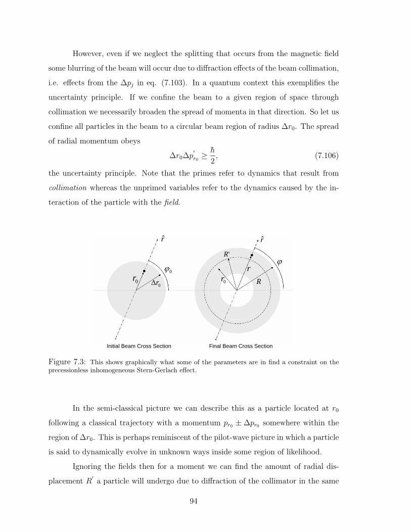
However, even if we neglect the splitting that occurs from the magnetic field
some blurring of the beam will occur due to diffraction effects of the beam collimation,
i.e. effects from the ∆pj in eq. (7.103). In a quantum context this exemplifies the
uncertainty principle. If we confine the beam to a given region of space through
collimation we necessarily broaden the spread of momenta in that direction. So let us
confine all particles in the beam to a circular beam region of radius ∆r0. The spread
of radial momentum obeys
∆r0∆p′
r0≥ h
2, (7.106)
the uncertainty principle. Note that the primes refer to dynamics that result from
collimation whereas the unprimed variables refer to the dynamics caused by the in-
teraction of the particle with the field.
0r0rΔ
0ϕ0r R
'R
rϕ
r r
Initial Beam Cross Section Final Beam Cross Section
Figure 7.3: This shows graphically what some of the parameters are in find a constraint on theprecessionless inhomogeneous Stern-Gerlach effect.
In the semi-classical picture we can describe this as a particle located at r0
following a classical trajectory with a momentum pr0 ± ∆pr0 somewhere within the
region of ∆r0. This is perhaps reminiscent of the pilot-wave picture in which a particle
is said to dynamically evolve in unknown ways inside some region of likelihood.
Ignoring the fields then for a moment we can find the amount of radial dis-
placement R′a particle will undergo due to diffraction of the collimator in the same
94

way that we found the dynamical displacement R. Assuming we can add the maxi-
mal amount of uncertainty to an initial radial momentum of pr0 = 0, i.e. initially no
spreading, we have
pr0 + ∆pr0 = ∆pr0 = mv′= m
(R
′
τ
)(7.107)
but with a maximum uncertainty state we also have
∆pr0 ≈h
2∆r0(7.108)
so
R′ ≈ hτ
2m∆r0. (7.109)
We interpret R′to be the maximum amount of spreading that will occur due
only to the collimation of a given beam of width ∆r0. We can see that if we make
the time of flight τ longer or if we made the beam more narrow, i.e. smaller ∆r0, the
spreading would be more pronounced.
Now, in order to assure ourselves that the spreading from the spin interactions
is observable against the inevitably spreading from collimation we require that
R > R′. (7.110)
Without this condition observation of the ISGE would be swallowed up in a blur.
Using our definitions for R and R′from eq. (41) and eq. (7.109) we get the
inequality
b∆r0T >m
e(7.111)
where all parameters that can be experimentally adjusted have been consolidated to
the left side. Only physical constants are on the right. The semi-classical description
tells us that this is the condition for an observable effect.
We have already discussed the field locally in the previous section. At r0 there
is apparently then a local SGE with a precession frequency of
ω =e|B|2m
=ebr02m
(7.112)
about the local field direction r.
95
This could average away the transverse deflections due to the transverse com-
ponents of the spin if it is allowed to operate long enough. Avoiding this gives us one
more experimental condition. We require
T ≈ 2π
ω=
4πm
ebr0(7.113)
where T is the time of interaction or the time the particle spends in the field. Putting
the value of T into the condition of eq. (7.111) we arrive at
r0 < 4π∆r0. (7.114)
If this condition is met then (1) precession is not a valid argument to discount the
measurement of transverse components in the field because it is too slow to sufficiently
average them away and yet (2) the spreading from spin effects will be observable
despite the spreading due to collimation. If we recall our interpretation of r0 as the
initial location of a particle within a beam spot of width ∆r0 it is seen that this
condition is always met.
This is an extremely interesting result but it must be qualified. (1) It follows
an approach that neglects the kinetic energy terms which amounts to dropping im-
portant derivatives from a differential equation in x-space. (2) It is a semi-classical
derivation so it is neither purely classical nor purely quantum. Its interpretation
stands therefore on unclear ground. Whatever concepts might be most useful from
either of the two regimes can be borrowed at will despite their mutual inconsisten-
cies. (3) From (2) all variable definitions are vague. (4) As an example of (3) the
momentum pr was used in one case as a definite value whereas in another case it
was said to uphold the uncertainty principle. Therefore, perhaps the inconsistency
of the result with the uncertainty principle is a function of the application of the
semi-classical representation and not of the phenomenon itself. (5) The B-field is
only approximate. (6) In conjunction with (1) the incident waves were assumed to
be infinite plane waves as stated in sections 6.2.1 so in actuality, even if all spin “up”
components go “out” and all “down” components go “in” nothing but an infinite blur
will be detected.
96

There are many other concerns that might be mentioned. These are sufficient
though to point out that this discussion provides an interesting test, namely the
method of this section, that might be applied under any circumstance using any
approach or interpretation. Even if physically wrong it is useful in teaching us about
our own misunderstandings of both interpretations of the representations and of the
representations themselves.
7.11 Other Representations
Amongst the representations explored in this chapter there are several other
possible representations by which we can view and assess the question of the ISGE
and precession in the standard SGE. We mention here a few of those that may be
beneficial.
7.11.1 Propagators
The Green’s function method outlined in section 6.9 maps source points in
space to field points in space. But this glossed over the time evolution of the system.
We have yet to do a solution that does not trivialize the time-dependence but allows it
to naturally evolve.6 Propagators can do this. They are similar to Green’s functions
but they map temporally past points to temporally present or future points.
[28] gives analytic expressions for the states ψ↑↓ in the coordinates (x, y, z)
which supposedly justifies its claim in section 6.12.2. However, as many of the techni-
cal details in its derivation are cited from other papers and have not been sufficiently
verified or interpreted we only mention this for completeness and to point out the po-
tential fruitfullness of the propagator method of [28] for describing the time evolution
in the ISGE.
6Section 6.10 is the closest we have come to this so far. Eq. (7.84) might be generalized fromassuming incident plane waves (vj = 0) to assuming some sort of incident packet (a spread in vj).
97
7.11.2 Numerical Methods
To this point no numerical investigation has been done. While representing
these problems numerically gives concrete and definite results they do not offer the
same sort of insight as does the explicit confrontation of detail that an analytic
approach offers. However, for a computer the PDEs that we have dealt with here
could be solved for specific choices of parameters. This would not only give us one
more perspective on the phenomenon of the ISGE but one that focused on results.
This could guide our work in other more revealing analytic approaches including the
ones discussed in this chapter. For example, it could provide an estimate for how
accurate eq. (7.46) is for the near-origin approximation of section . 7.5.7. For this
reason numerical methods should be pursued in the future.
7.11.3 Perturbation Theory
Often a portion of a system can be designated as small. Using perturbation
methods these small effects can be eventually accounted for. This generally yields
approximate but often accurate results. Although one of the defining characteristics
of the ISGE is the equal treatment of field components there are several other pertur-
bation techniques that might be applied to solving the ISGE as was the Born method
in section 6.9.2.
7.11.4 Bohmian Mechanics
Because we desire to understand the inner workings of the measurement pro-
cess it is difficult to apply standard quantum techniques to gain understanding. In
a field that is formed by measurement axioms7 how does one objectively study the
nature of measurement itself? The methods of quantum mechanics have been effec-
tively designed and interpreted to match experimental results or potential results, not
processes.
There has been relatively little done with the other approaches that claim to
give an accounting of the behind-the-scenes dynamics of the measurement process
7Note the discussion of the “collapse” and “cut” axioms in section 3.2.2.
98

but they do exist. Many have applied the mechanics first introduced by de Broglie in
1927 and formalized by David Bohm in 1952 to inquiries of the SGE. In such cases
the actual dynamics of both the position and spin orientation of the particles can be
continuously and consistently described [37], [38], [13], [12]. This has even been done
using the representational algebra of section 7.7 to account for relativistic effects [39].
Insightful investigations of the sort proposed by Bohm should be extended to
the case of the ISGE. Like many other representations they have the potential to offer
unique insights into the operation of measurement and the SGE in general.
99

100

Chapter 8
Conclusions
There has been an overarching tension in all that we have done in this thesis.
It arises from the fact that while representations are necessary in order for rational
communication and comprehension they also necessarily alter the perceived behavior
of the phenomena they represent. They carry an accompanying value system and set
of assumptions. In the case of the traditional SGE these values and assumptions have
not been explicitly identified in the past because of its axiomatic role in the modern
interpretation and practice of quantum mechanics. In Chapter 5 we attempted to
show how this has limited our understanding, or possibility for understanding, in
various ways and proposed a study of the ISGE. The question then becomes, “How
does one study a phenomenon independent of of its representation?” In this thesis we
have used several different techniques in an effort to understand the SGE, and more
particularly the ISGE, on a deeper level.
8.1 The Method of Relativity
Despite the multiplicity of specific methods that we have used our overall
approach is not that different from the general methodology of Einsteinian relativity.
Instead of being confused by the relative nature of the several possible points of view
that can be taken to solve a single problem we have deliberately moved between these
“frames of reference” in order to study nature on a level independent of the frames
themselves. That is, by honestly recognizing our relative knowledge we can approach
more absolute knowledge.
101
In more concrete language we have approached the ISGE using several differ-
ent methods. Each method necessarily involved some simplifying assumptions and
approximations. By comparing the effects of these simplifications, i.e. the results,
between several methods we were able to conclude as to which behaviors belong to
the method and which belong to the phenomenon. By comparing several techniques
we gained confidence in our conclusions.
8.2 Our Results
For example, in our thematic account two distinct momenta were found using
the rest frame of the particles in the beam. We noted how this amounts to the
assumption of incoming plane waves. This assumption was also made in other sections
with similar results. However, using the Heisenberg representation made it more
explicit so that one could perhaps lift the assumption in graded steps thus more
closely returning to exact solutions.
In our use of differential equations we did not make the assumption of incoming
plane waves. It did however show us the effect of not having an asymptotically finite
field. Using the integral equations provided by Green’s functions provided for both
these issues: we could address the asymptotic behavior of the field without having to
assume incoming plane waves.
The Heisenberg representation also allowed us to treat the time-dependence in
a more natural way and using the Clifford algebra Cl3 we found a result that which
seemed to emphasize the rotations of a local precession and not the discreteness in
the momenta. Cl3 also gave us a way to convert systems of coupled equations into a
single equations in which the separation of variables might be useful.
Some of our most significant results have had to do precession because it is
so vital to the standard description of the SGE. We saw how the effect of precession
can be explicitly represented as a clearly mathematical trick without any necessary
recourse to the physical picture of rotating spin vectors (section 7.1.3). This doesn’t
help our intuition but by abstracting away from physical pictures it allows us a view
of its mathematical structure. Again, with this knowledge we could reconstruct and
102
study the effects of precession, gradually moving from the ISGE to the SGE, by
keeping higher and higher order terms in the expansion eq. (7.7).
We also saw how it was precession that by and large justified the usual in-
terpretation of the uncertainty principle in Stern-Gerlach measurement by averaging
away incompatible components. However, we saw that the precessionless ISGE could
require us to use a more definite notion of uncertainty as the appearance of any local-
ized spot on the detecting plate seems to violate its usual interpretation (see section
5.5.3).
Thus, the ISGE, which appears to be only a local version of the traditional
SGE in which the spin separations occur along a radial axis as defined by the initial
position of the particle, has opened the door for a clearer study of both the theory
and interpretation of physical science. We believe there are still several interesting
and unanswered questions as to the correct interpretation of the SGE. Being very
subtle and “relative” issues these may be pursued using the methodology of relativity
as we have used it here.
8.3 The Dangers of an Inadequate Philosophy
Perhaps one of the most interesting conclusions of applying methods involving
several representations is not the absolute knowledge that comes out but that the
apparent fact that there is absolute knowledge. For this reason we cannot be too
content with the prevalent “it works” attitude although it may be necessary for the
purposes of instruction. That is, “it works” should only serve as a temporary justifi-
cation for pursuing knowledge and not as a permanent replacement. Whether or not
something “works,” which is a relative term, theoretical and analytical studies should
be encouraged - using many different representations - as only they provide explicit
conceptual confrontation with all the details of nature. This will allow us to form a
more accurate picture of physical processes, for, as we hinted at in section 2.1
Without abstract ideas...‘you would not be able to deal with concrete,
particular, real-life problems. You would be in the position of a new-born
infant, to whom every object is a unique, unprecedented phenomenon...As
103

a human being [we] have no choice about the fact that [we] need a phi-
losophy. [Our] only choice is whether [we] define [our] philosophy by a
conscious, rational, disciplined process of thought and scrupulously log-
ical deliberation - or let [our] subconscious accumulate a junk heap of
unwarranted conclusions, false generalizations, undefined contradictions,
undigested slogans, unidentified wishes, doubts and fears, thrown together
by chance, but integrated by [our] subconscious into a kind of mongrel
philosophy and fused into a single,solid weight: self-doubt, like a ball and
chain in the place where [our] minds’s wings should have grown. [3] (p.
1-2)
In summary, the search for a more complete and consistent understanding of
the SGE has led us to an understanding, not only of the SGE and precession, but
more generally of the process of representation. We have seen that in the act of
representing a phenomenon for communication or study there is an inherent tension
contributes can contribute to our progress. In research this is manifest as the tension
between accurate historical accounts and clearly formed thematic ones, between the
physical and analytical justifications of our approximations, between the the realist
and positivist interpretations of physics, between the x and p representations, be-
tween mutually inconsistent approximation methods, etc. In physics education and
teaching this tension lies in the necessary balance of both clear and accurate commu-
nication. In any case we have seen the value of not only understanding the dispar-
ities of our representations but also in accepting and using them for our advantage
and progress. Thus, because of the inadequacy and necessity of our representations,
progress-oriented research and teaching require that we master the art of mediation.
104
Bibliography
[1] D.J. Griffiths, Introduction to Quantum Mechanics, (Prentice Hall, Upper SaddleRiver, 1995).
[2] T.S. Kuhn, The Structure of Scientific Revolutions, (The University of ChicagoPress, Chicago, 1996).
[3] A. Rand, Introduction to Objectivist Epistemology, (Meridian, New York, 1990).
[4] L. Peikoff, Objectivism: The Philosophy of Ayn Rand, (Meridian, New York,1993).
[5] J. Cushing, Quantum Mechanics: Historical Contingency and the CopenhagenHegemony, (University of Chicago, Chicago, 1994).
[6] E.A. Burt, The Metaphysical Foundations of Modern Science, (Humanity Books,New York, 1999).
[7] J.C. Leon, Science and Philosophy in the West, (Prentice Hall, Upper SaddleRiver, 1999).
[8] A. Grometsein, The Roots of Things, (Prentice Hall, Upper Saddle River, 1999).
[9] L. Ballentine, Quantum Mechanics, (Prentice Hall, Englewood Cliffs, 1990).
[10] A. Peres, Quantum Theory: Concepts and Methods, (Kluwer Acdemic Publishers,Dordrecht, 1993).
[11] J.S. Bell, Speakable and Unspeakable in Quantum Mechanics, (Cambridge Uni-versity Press, Cambridge, 2004).
[12] D. Bohm and B.J. Hiley, The Undivided Universe, (Routledge, London, 1993).
[13] P. Holland, The Quantum Theory of Motion: An Account of the de-Broglie-BohmCausal Interpretation of Quantum Mechanics, (Cambridge University Press, Cam-bridge, 1995).
[14] H. Kragh, “Max Planck: the reluctant revolutionary,” Physics World, retrievedon May 10, 2005.
[15] P.M. Parker, “The Bohr-Sommerfeld Model of the Atom,” PHYSNET, retrievedon May 10, 2005.
105

[16] B. Friedrich and D. Herschbach, “Stern and Gerlach: How a Bad Cigar HelpedReorient Atomic Physics,” Physics Today, 53-59 (2003).
[17] Image at retreived on June 13, 2005.
[18] T.E. Phipps and J.B. Taylor, “The magnetic moment of the hydrogen atom,”Phys. Rev. 29, 309-320 (1927).
[19] F. Aaserud and D. Favrholdt eds., Niels Bohr Collected Works vol. 10, (Elsevier,Amsterdam, 1999).
[20] N. Bohr, Atomic Physics and Human Knowledge, (John Wiley & Sons, Inc., NewYork, 1958).
[21] W. Heisenberg, Physics and Philosophy: The Revolution in Modern Science,(Harper and Row, New York, 1958).
[22] R. Feynman, The Character of Physical Law, (MIT Press, Cambridge, 1965).
[23] O. Stern, “Ein Weg zur experiemtellen prufung der Richtungsquantelung imMagnetfeld” Zeits.Phys. 7, 249-253 (1921).
[24] W. Pauli, (1932), “Les thories quantiques du magntisme. L’lectron magntique,”in 6ime Conseil de Physique Solvay, Le Magntisme, Bruxelles,1932, pp.175-280,(Paris).
[25] P. Alstrom, P. Hijorth, and R. Mattuck, “Paradox in the classical treatment ofStern-Gerlach experiment,” Am. J. Phys. 50 (8), 697-698 (1982).
[26] S. Singh and N. K. Sharma, “Comment on ‘Paradox in the classical treatmentof the Stern-Gerlach experiment’,” Am. J. Phys. 52 (3), 274-275 (1984).
[27] P.A. Tippler and R.A. Llewellyn, Modern Physics, (W.H. Freeman and Company,New York, 2003).
[28] M.O. Scully, W.E. Lamb Jr., and A. Barut, “On the Theory of the Stern-GerlachApparatus,” Found. of Phys. 17 (6), 575-583 (1987).
[29] G. Potel, et. al., “Quantum mechanical description of Stern-Gerlach experi-ments,” retrieved on September 29, 2004.
[30] J. Larsen, B.M. Garraway, and S. Stenholm, “Transient effects on electron spinobservation,” Phys. Rev. A 69 (032103), (2004).
[31] G.B. Arfken and H.J. Weber, Mathematical Methods for Physicists, (HarcourtAcademic Press, San Diego, 2001).
[32] P.M. Morse and H. Feshbach, Methods of Theoretical Physics Parts I,II,(McGraw-Hill, New York, 1953).
106

[33] E. Merzbacher, Quantum Mechanics, (John Wiley & Sons, Inc., New York, 1998).
[34] E.S. Cheb-Terrab, “Solutions for the general, confluent and biconfluent Heunequations and their connection with Abel equations,” J. Phys. A: Math. Gen. 379923-9949 (2004).
[35] A. Ronveaux, ed., Heun’s Differential Equations, (Oxford University Press, Ox-ford, 1995).
[36] C. Doran and A. Lasenby, Geometric Albegra for Physicsits, (Cambridge Univer-sity Press, Cambridge, 2003).
[37] C. Dewdney, P.R. Holland, and A. Kyprianidis, “What happens in a spin mea-surement?” Phys. Lett. A 119, (6) 259-267 (1986).
[38] C. Dewdney et. al., “Spin and non-locality in quantum mechanics” Nature 336,536-544 (1988).
[39] A. Challinor, et al. “A relativistic, causal account of a spin measurement,” Phys.Lett. A 218, 128-??? (1996).
[40] F. Weinet, “Wrong Theory–Right Experiment: The Significance of the Stern-Gerlach Experiments,” Stud. Hist. Phil. Mod. Phys. 23 (1) 75-86 (1995).
[41] B. Friedrich and D. Herschbach, “Space Quantization: Otto Stern’s Lucky Star,”Daedalus, 127, (1) 165-192 (1998).
[42] D. Kleppner and R. Jackiw, “One Hundred Years of Quantum Physics,” Science,289, 893-898, August 11 2000.
107