research 303 - a review of the hdm/dtims pavement … · a review of the hdm/dtims pavement models...
TRANSCRIPT
A review of the HDM/dTIMS pavement models based on calibration site data
T.F.P. Henning, S.B. Costello, T.G. Watson, MWH NZ Ltd Land Transport New Zealand Research Report 303

ISBN 0-478-28715-1 ISSN 1177-0600
© 2006, Land Transport New Zealand PO Box 2840, Waterloo Quay, Wellington, New Zealand Telephone 64-4 931 8700; Facsimile 64-4 931 8701 Email: [email protected] Website: www.landtransport.govt.nz Henning, T.F.P.1, Costello, S.B.1, Watson, T.G.1 2006. A review of the HDM/dTIMS pavement models based on calibration site data. Land Transport New Zealand Research Report 303. 123pp. 1 MWH New Zealand Ltd, PO Box 12 941, Penrose, Auckland
Keywords: calibration, crack initiation, dTIMS, HDM, LTPP, pavement performance, road deterioration, roughness model, rutting, surface texture

An important note for the reader Land Transport New Zealand is a Crown entity established under the Land Transport Management Act 2003. The objective of Land Transport New Zealand is to allocate resources and to undertake its functions in a way that contributes to an integrated, safe, responsive and sustainable land transport system. Each year, Land Transport New Zealand invests a portion of its funds on research that contributes to this objective. The research detailed in this report was commissioned by Land Transport New Zealand. While this report is believed to be correct at the time of its preparation, Land Transport New Zealand, and its employees and agents involved in its preparation and publication, cannot accept any liability for its contents or for any consequences arising from its use. People using the contents of the document, whether directly or indirectly, should apply and rely on their own skill and judgement. They should not rely on its contents in isolation from other sources of advice and information. If necessary, they should seek appropriate legal or other expert advice in relation to their own circumstances, and to the use of this report. The material contained in this report is the output of research and should not be construed in any way as policy adopted by Land Transport New Zealand but may be used in the formulation of future policy

Acknowledgment This project has been co-funded by Land Transport New Zealand and Transit New Zealand (Transit). In addition to direct financial contribution Transit has also provided the data for model calibration and model development work.

5
Contents
Executive summary ........................................................................................... 7
Abstract............................................................................................................13
1. Introduction ............................................................................................15 1.1 Background to the research .................................................................15 1.2 Scope of the report.............................................................................15
2. Background to the study ..........................................................................16 2.1 Long-term pavement performance studies in New Zealand .......................16 2.2 Research objectives ............................................................................16 2.3 LTPP Data .........................................................................................17
3. Calibration analysis approach...................................................................20 3.1 An important note on HDM models........................................................20
3.1.1 The philosophy behind HDM models ............................................20 3.1.2 Data-driven models ..................................................................20
3.2 Calibration levels according to HDM.......................................................21 3.3 Analysis approach for HDM calibration level 2 .........................................22
3.3.1 Crack initiation ........................................................................22 3.3.2 Crack progression models..........................................................24 3.3.3 Rut progression .......................................................................24 3.3.4 Rutting calibration methodology .................................................26 3.3.5 Surface texture........................................................................27 3.3.6 Roughness progression .............................................................29 3.3.7 Roughness model calibration .....................................................30 3.3.8 Pothole initiation and progression ...............................................32
3.4 Analysis approach for HDM calibration level 3 – Adaptation.......................32
4. Crack initiation.........................................................................................34 4.1 HDM level 2 calibration........................................................................34
4.1.1 Cracking data used for the level 2 calibration ...............................34 4.1.2 Results ...................................................................................35
4.2 A Review of the cracking model format ..................................................36 4.2.1 Crack initiation data for the model review....................................36 4.2.2 Refining the existing HDM model format ......................................38 4.2.3 Variable analysis ......................................................................39 4.2.4 Multivariate analysis .................................................................44 4.2.5 Linear model (LM) regression analysis results...............................45 4.2.6 Generalised linear model (GLM)..................................................47
4.3 Summary of modelling review ..............................................................51
5. Texture ....................................................................................................53 5.1 A review of the simplified texture model ................................................53
5.1.1 Description of data ...................................................................53 5.1.2 Variable analysis ......................................................................54 5.1.3 Standardised analysis ...............................................................54
5.2 Testing the texture model on the basis of LTPP data ................................55

6
6. Rutting.................................................................................................... 57 6.1 Rut depth measurements and data....................................................... 57 6.2 Calibrating the existing HDM rutting models .......................................... 58
6.2.1 HDM-III rut progression calibration results .................................. 58 6.2.2 HDM-4 rut progression calibration results.................................... 60
6.3 Refining the rut progression model....................................................... 62 6.3.1 Description of the data ............................................................. 62 6.3.2 Variable analysis ..................................................................... 62 6.3.3 Linear model (LM) regression analysis results .............................. 65 6.3.4 Future development requirements for rut progression model.......... 67
6.4 Rut depth standard deviation............................................................... 67
7. Roughness .............................................................................................. 70 7.1 LTPP roughness data .......................................................................... 70 7.2 A review of the roughness model ......................................................... 71
7.2.1 Environmental component ........................................................ 71 7.2.2 Structural component .............................................................. 71 7.2.3 Incremental change caused by rutting ........................................ 72
7.3 Proposed changes to the roughness model. ........................................... 72
8. Recommendations ................................................................................... 75 8.1 The future of the New Zealand LTPP sections ......................................... 75 8.2 Investigate the rapid failure stage for roughness and rutting progression ... 75 8.3 Introducing uncertainty and statistical distribution in some models ........... 76
9. References .............................................................................................. 77
Appendices ...................................................................................................... 79

Executive summary
7
Executive summary
The aim of this research, carried out in 2005, was primarily to test the current pavement
deterioration models adopted in the New Zealand system. Most of these models were
adopted from HDM-III and HDM-4, but some locally developed models were also tested.
The model calibrations performed could be divided into the following categories:
• Calibration Level 2 – adjustment of the calibration coefficient. For this calibration
level, all other model coefficients were kept at the default level.
• Calibration Level 3 (model adjustment) – regression to obtain the best model
coefficients for New Zealand conditions. The original model format is kept and the
values of all the model coefficients are adjusted in order to minimise the error
between the predicted and the observed data points.
• Calibration Level 3 (new model format) – data-driven models are developed from
first principles based on the Long Term Pavement Performance (LTPP) data.
In all cases, care was taken to ensure that sufficient and appropriate data were used
during the analysis. For example, given the relatively young age of the LTPP programme,
more data had to be sourced in order to perform the calibration of the cracking model. It
should also be noted that only the priority performance prediction model was calibrated
during this study. There are also other models, such as the potholing model, which have
not been addressed in this report, but which have been included in the overall model
developments for New Zealand. A summary of the model calibration results is provided in
the following sections.
Crack Initiation
In agreement with engineering judgement, this report again emphasised the importance
of crack initiation. It signals a significant turning point in the behaviour of the pavement,
and is often the starting point of accelerated deterioration. It has also been confirmed
that a cracked pavement will have shorter expected life even if it is resurfaced. The crack
initiation calibration included all the calibration steps and the results are presented in
Table ES1.

A REVIEW OF THE HDM/DTIMS PAVEMENT MODELS BASED ON CALIBRATION SITE DATA
8
Table ES1 Summary of the crack initiation calibration results.
Calibration Level/Method
Results Error/Accuracy
Level 2 –
Adjusting Calibration Coefficients
Regional Classification
High and Moderate Low and Limited
Kci 0.49 (0.52*) 0.59 (0.64*)
Error – Default 194 477
Error – Calibrated 27 160
Note: Calibration was performed on LTPP data. Values in brackets resulted from calibration
performed on regional data
Level 3 – Adjusting
Model Coefficients
Default HDM-4 Model Coefficients
a0 a1 a2 a3 a4
13.2 0 20.7 20 0.22
Adjusted HDM-4 Model Coefficients for Chip Seals
a0 a1 a2 a3 a4
8.3 0 18.54 0.01 0.34
17597.7
6697.9
Level 3 – New Model
Format (Linear Model)
For PCA = 0 (sections not cracked before resurface)
⎥⎦
⎤⎢⎣
⎡ −−=
log(AADT)*OT)0.08log(HT+T)0.3log(AADOT)1.25log(HT5.7
exp*KciICA
For PCA > 0 (sections were cracked before resurface)
⎥⎦
⎤⎢⎣
⎡ −−=
log(AADT)*log(HTOT)*0.08+DT)0.47log(AAOT)0.68log(HT4.6
exp*KciICA
where:
ICA is the crack initiation time in years after the surface is constructed
HTOT is the total surface thickness (in mm) of all the layers
AADT is the annual average daily traffic
5157
Level 3 – Generalised
Model
{ }⎥⎦
⎤⎢⎣
⎡⎟⎟⎠
⎞⎜⎜⎝
⎛+−−
=++=
SNPLog(HTOT)Log(AADT)(0,1)stat.pca 0.141AGE2-1)p(stat.aca
655.0275.0455.0)440.3,062.5(
exp1for
where:
p(stat.aca) is the probability of a section being cracked
AGE2 is the surface age in years, since construction
stat..PCA is the cracked status before resurfacing (0 or 1 for not cracked or cracked)
HTOT is the total surface thickness (in mm) of all the layers
AADT annual number of equivalent standard axles (millions/lane)
SNP is the modified structural number

Executive summary
9
Both the linear model and the generalised model deviate substantially from the original
HDM model. The main reason for the significant difference is that the latter two models
are purely data-driven. They suffer one big disadvantage in the sense that they can only
be adopted within the environment for which they were developed. It is thus
recommended that all the model formats are tested on any network where they are
applied. However, this would not be an onerous task and it could be easily performed for
all state highways.
Given the advantages of the logistic model as presented in the report, it is recommended
that this model format is adopted for New Zealand roads. Part of this adoption will include
testing the model for other regions and formulating the practical inclusion of the model in
the decision process of the pavement management system.
Texture
In a previous study by Transit in 2003 a simplified texture model was developed as an
alternative to the HDM texture model. That report recommended a different approach for
determining model coefficients depending on the availability of data. This study has
confirmed the model format to be appropriate, but has recommended that different
coefficients should be developed for each chip size, but not for individual regions. The
recommended model coefficients are presented in Table ES2.
Table ES2 Recommended model coefficients
Type a0 Std. Error a1 Std. Error
AC 1.024727 0.164577 −0.01889 0.009675
CHIP.G2 4.314283 0.101516 −0.12662 0.006757
CHIP.G3 4.158183 0.071979 −0.13461 0.004663
CHIP.G4 3.407922 0.177842 −0.10949 0.011158
CHIP.G5 3.479998 0.120092 −0.12425 0.007992
CHIP.G6 2.319671 0.242437 −0.07236 0.015257
OG 1.182618 0.142981 0.005555 0.00809
The model format and coefficients were tested on the calibration SLP data and a
reasonably good fit was established.
The base texture model seems to be yielding satisfactory results. However, more work
needs to be completed in the area of the rapid deterioration phase of texture loss
(flushing model). With this model, more understanding needs to be developed on the
interaction between variables such as traffic, and the surface characteristics such as total
thickness of the surface.
Rutting
The rut depth progression has been calibrated according to both the HDM-III and HDM-4
model. The resulting coefficient from these analyses are presented in Table ES3.

A REVIEW OF THE HDM/DTIMS PAVEMENT MODELS BASED ON CALIBRATION SITE DATA
10
Table ES3 Rut depth progression calibration results.
HDM-III HDM-4
Sensitivity Risk Area1
Calibration Coefficient
(Krp)
Error Function (RMSE)2
Calibration Coefficient (Krp)
Error Function (RMSE)2
Low and Limited
0.87 23,333 (30,746) 1.03 2,719 (2,729)
Medium and High
0.81 729 (1,346) 0.98 931 (933)
All Data 0.84 22,583 (32,092) 1.01 3,658 (3662)
Note: 1 The data was not sufficient (i.e. nor enough data points) to perform successful calibration on individual sensitivity risk areas
2 The values in brackets indicate the error function result using the default calibration coefficient (Krp=1). RMSE = root mean square error
An attempt was made to improve the rutting model format, but the model could not be
improved. However, it was observed that for most of the pavement life a fairly constant
rate of rutting progression occurs (this equates to approximately 0.3 mm per year based
on the LTPP data). The recommended work for the rut progression model includes:
• Investigate rut progression model forms on the CAPTIF data. Two major trends
must be investigated:
- Determine the factors contributing towards stable rut progression observed
during most of the pavement life. In particular see if the CAPTIF data conforms
to the constant 0.3 mm rut progression of pavements. - Determine the factors contributing towards a pavement that starts accelerated
deterioration that includes a rapid rut progression. • Further analysis into tracking rutting on individual sections over time. As the LTPP
data become available for longer time periods, this analysis would become more
useful. By combining trends from the LTPP data and the CAPTIF data, it may also
be possible to develop model formats from basic principles.
Roughness
The roughness model calibration could not be performed based on the current available
data. The data did, however, confirm that the HDM-4 model format does not reflect the
actual behaviour of most pavements in New Zealand. The model suggests a relatively
long period of the pavement life during which the deterioration is slow. Then it reaches a
stage of rapid deterioration. The aim of the future model development would be to predict
the timing when the rapid deterioration commences. Insufficient LTPP data existed to perform the desired model development. Only a limited
number of sections have reached the rapid deterioration stage. It is recommended that
some CAPTIF data be applied to develop the model format. In addition to this, extended
LTPP data can then be used to confirm the model behaviour on the state highways as it
becomes available. The recommended work includes:

Executive summary
11
• Investigate the roughness reduction trend after construction. The aim is to
determine how much of this reduction is actual smoothing of the pavement versus
the perceived roughness reduction caused by measurement technique.
• Confirm the roughness trend during the gradual deterioration phase with more LTPP
and CAPTIF data.
• Determine the factors contributing towards the initiation of the rapid deterioration
phase of roughness progression.
A new relationship for the rut depth standard deviation is proposed:
[ ]0.9369RDM)0.8804log(exprds −=
However, this model will suffer the same limitation as the previous model since it is a
function of the mean rut depth (RDM). The proposal is to develop a new model format
from first principles which will not be reliant on the mean rutting.
Recommended further work
The future of the New Zealand LTPP sections
This report has demonstrated that the level of data collection accuracy is appropriate for
calibration and pavement model development. Some intuitive trends with some models
(such as roughness) have been confirmed for the first time since the appropriate level of
data accuracy existed. However, this study has also highlighted the need for further
model development based on individual section data. It has been suggested that some of
the models such as roughness and rutting could be developed utilising some CAPTIF data,
but ultimately could only be confirmed with the LTPP data.
Furthermore, the report has highlighted the significance of the rapid failure stages of
pavement deterioration modelling. In order to understand the behaviour during rapid
deterioration better, more data during this stage is needed.
It is therefore recommended that the LTPP surveys continue on both the Transit and local
authority networks. It is difficult to predict the time required, but it is estimated that the
surveys should continue for at least another five years.
In terms of the current data collection precision and accuracy requirements, it is
recommended that the current standard be maintained.
Investigate the rapid failure stage for roughness and rutting progression
As a next stage to this research, a proposal was accepted for the 2005/06 Land Transport
New Zealand Research Programme. This study is aimed at linking the LTPP and the
CAPTIF programmes. The objectives of this research are explained in the extract from the
research proposal:
Linking the outputs from CAPTIF with the LTPP study is the next logical step
towards building on the understanding of pavement performance/
deterioration under New Zealand conditions. Comparing field performance

A REVIEW OF THE HDM/DTIMS PAVEMENT MODELS BASED ON CALIBRATION SITE DATA
12
(LTPP) with the accelerated load performance (CAPTIF) will significantly
increase the confidence in outputs from both these programs. The specific
objectives of the study include:
1. Calibration coefficients and new model formats have been developed
based on the Transit LTPP data (Transfund Research Programme
04/05). The first objective would be to confirm and improve the model
format and results based on existing CAPTIF data.
2. To develop relative performance factors for different treatments and
material types, similar to the work completed in Australia (Martin
2004). It should be appreciated that the data from both programmes
will greatly extend the range of applicability of both programmes.
3. To gain a better understanding of the environmental impact on
pavements. The LTPP sections are subjected to normal climatic
influences whereas the CAPTIF testing was conducted under controlled
conditions. It is therefore possible to investigate the specific
environmental impacts on pavement performance, something which is
relatively complex to do based on LTPP work alone.
4. Confirm CAPTIF life cycle and mass limit study results with the LTPP
performance data.1
An obvious emphasis of this study would be to increase the understanding of the
deterioration of the pavement during the rapid failure stages.
Introducing uncertainty and statistical distribution in some models
According to some network experience combined with engineering observations, some of
the pavement behaviour cannot be explained according to deterministic model formats.
For example, this report has suggested a generalised linear model format for predicting
cracking. Likewise, defects such as potholing and failures (shoving) would be easy to fit
according to some statistical distribution such as a Proportional Intensity Model. This
change in modelling approach would not be transferable like the HDM approach. However,
it would produce modelling outcomes that more closely resemble actual behaviour in New
Zealand. It is recommended that this development is undertaken as part of the dTIMS CT
development consortium tasks, since it will optimise the input from all practitioners in
New Zealand.
1 Research Proposal: Benchmarking pavement performance between Transit’s LTPP & CAPTIF
programmes 05/06 Research Round. MWH New Zealand Ltd.

Abstract
13
Abstract
New Zealand started a Long-Term Pavement Performance (LTPP) programme
on the State Highway network during 2000. This report presents the first
concrete outcomes from the calibration analysis, undertaken in 2005.
The cracking model, particularly the crack initiation model, is one of the most
crucial in the simulation of pavement deterioration. It contributes to many
other pavement models such as roughness and rutting. A comprehensive
process of data analysis was carried out including a traditional calibration
coefficient adjustment of the HDM-4 model, adjustment of all HDM model
coefficients based on maximum likelihood estimation, linear model
regression, and logistic model development. The same process was followed
for the texture and rut progression model. The simplified model format of the
texture model has been calibrated. Reviewing the model format of the rut
progression has been less successful due to data shortages but a path for the
next stage of development is proposed.
This research from 2005 highlights the merits of the various calibration and
model-development techniques as well as providing a comparison of the
model outcomes. This is done both in terms of their accuracy in predicting
crack occurrence on a network and their applicability to networks outside of
the development area.

A REVIEW OF THE HDM/DTIMS PAVEMENT MODELS BASED ON CALIBRATION SITE DATA
14

1. Introduction
15
1. Introduction
1.1 Background to the research
The intent of this research was to review the major pavement deterioration models used
in the New Zealand Deighton's Total Infrastructure Management System (dTIMS).The
New Zealand dTIMS system was adopted during 1999 and consists of the following
components:
• a software analysis platform, dTIMS, which was superseded by a later version,
dTIMS CT in 2004,
• an analysis framework developed to simulate New Zealand best practice in
maintenance decision making,
• pavement deterioration models, which are based on the World Bank’s Highway
Design and Maintenance models(HDM-III), HDM-4 and some locally developed
models,
• all supporting software required to perform data preparation and reporting.
This research was commissioned through the Land Transport New Zealand Research
Programme and was carried out in 2005. It is the first calibration study aimed at
reviewing the HDM models for New Zealand conditions. It will also set the basis for
further research in this area.
1.2 Scope of the report
The purpose of this report is not only to report the findings from the calibration analysis
and model development, but also to provide a strategy for future calibration needs. This
strategy includes a recommendation regarding the recommended analysis approach.
The report starts with a brief summary of calibration levels and the analysis approach that
has been considered during the analysis work. The existing HDM approach was adhered to
wherever possible. However, where appropriate, alternative methods were recommended
based on New Zealand and other international experience.
The report then documents the findings from a calibration performed on the major
performance models. As a first attempt only the calibration coefficients are adjusted. This
section highlights all the issues related to a poor match between the prediction model and
the actual behaviour of the pavement. Outcomes from this section include the provision of
regional calibration coefficients, further model development areas and proposed
calibration processes.
Subsequently, the model formats are reviewed from basic principles. Significant variables
are identified according to their influence on the dependent variables. Inter-relationships
of variables are investigated leading towards the definition of new model formats. Where
possible new model formats are compared with adjusted HDM models.
The last section makes recommendations and puts into place a 'road map' for future
modelling calibration needs.

A REVIEW OF THE HDM/DTIMS PAVEMENT MODELS BASED ON CALIBRATION SITE DATA
16
2. Background to the study
2.1 Long-term pavement performance studies in New Zealand
During the implementation of the asset management system in New Zealand, the HDM
models were adopted with the knowledge that they would require calibration once the
appropriate data became available. The need for calibration has also been highlighted in a
number of modelling reports completed for both Transit New Zealand (Transit) regions
and local authorities. As a result two Long-term Pavement Performance (LTPP)
programmes were initiated:
• Transit established 63 LTPP sections on the state highways. An annual condition
survey is performed on these sections and during April 2005 these sections were
surveyed for the fourth time.
• Land Transport New Zealand, in association with 21 local authorities, established 82
sections on typical local authority roads in both urban and rural networks.
This report documents the calibration results based on the 2004/05 analysis round,
formulates recommended calibration procedures, and reviews the appropriateness of the
local authority data based on the past two years of survey data.
2.2 Research objectives
According to the HDM modelling philosophy, pavement deterioration models are provided
with a set of default calibration coefficients. The intention of these coefficients is to be
able to adjust the models for different climatic conditions. For example, most of the
technical development work on the original HDM models was undertaken in Brazil and the
climate and road building materials of New Zealand differ significantly from those in
Brazil. In theory, the calibration coefficients are provided to cater for these differences. In
a wetter climate with more sensitive soils, as exists in New Zealand, the expectation is
that the calibration coefficients would need to be altered to reflect these conditions.
Some initial calibration analysis suggested that, for some defects, changing the calibration
coefficients alone may not give satisfactory results. Henning & Tapper (2004) indicated
that some models such as the roughness progression do not necessarily follow the model
format as described by HDM. Figure 2.1 illustrates an example of a pavement
deterioration model that required a model form change in order to reflect the actual
pavement deterioration.

2. Background to the study
17
ActualObservations
from FieldMeasurements
Standard HDMModel Form
(Un-Calibrated)
New ModelForm
Resultingfrom this
Experiment
New PavementDeteriorationModel Form
Pave
men
tC
ondi
tion
Time Figure 2.1 Example of changing the model format to fit actual data.
The main purpose of this research is to improve the fundamental understanding of
pavement performance/deterioration including the regional variation. This was achieved
through addressing the following objectives:
• To complete a full review of the pavement deterioration models used in dTIMS. This
objective included the provision of calibration coefficients for the different climatic
areas in New Zealand (Level 2 calibration).
• Should the analysis suggest a need for calibration beyond adjusting the calibration
coefficients, to develop new model forms.
• To test the appropriateness of the local authority sections and data in terms of the
defined experimental design.
• To develop a medium-term research strategy for model calibration in New Zealand.
2.3 LTPP data
The LTPP sections consist of 300 m-long sections selected according to a design matrix
that ensures representative samples from different climatic areas, traffic, pavement, and
network types. These sections are established on existing networks across the state
highway and local authority network. On some of these sections (sterilised sections), no
maintenance is allowed other than safety-related maintenance (e.g. pothole patching).
The remaining sections are subject to normal maintenance practices for that particular
network.
The LTPP data consist of inventory, as-built, traffic, strength, maintenance, and condition
data. A summary of the data sources is provided in Table 2.1.

A REVIEW OF THE HDM/DTIMS PAVEMENT MODELS BASED ON CALIBRATION SITE DATA
18
Table 2.1 LTPP data sources.
Data Item Description Data Source
Inventory Pavement layer and surface details Originally from RAMM* and other records but further validated by test pit information
Rainfall Rainfall data Purchased from NIWA
Pavement Strength
Analysed Falling Weight Deflectometer Data (FWD)
Annual FWD Surveys spaced at 50 m intervals
Traffic Collected traffic data (AADT**) and the estimated percentage of vehicle type distribution
RAMM (for local authorities) and the Transit Traffic Management System (TMS) for state highways
Maintenance Records
Detail on any maintenance recorded on the LTPP sections
Submitted through software provided
Condition Data Manually measured condition items such as roughness, rutting, texture and visual defects
Sourced through a condition survey contract
* averaged annual daily traffic ** road asset management and maintenance system
The condition surveys for both the programmes (Transit LTPP and Land Transport New
Zealand) are secured through performance-specified survey contracts. According to these
contracts, the accepted tolerances on the data collection precision are specified and the
contractor nominates the instruments to be used. Henning et al. (2004a) and Transit
(2001) documented the survey process along with the contracted technical specifications.
The contractor opted to use the following instruments for the condition surveys.
Roughness The roughness is measured using an ARRB Walking Profilometer. Three
measurements are conducted in each wheel path to achieve the required repeatability.
Rutting The transverse profile is measured with a self-driven Transverse Profile Beam
(Figure 2.2). The transverse profile is measured at 10 m intervals and two measurements
are conducted to achieve the required repeatability. The rut depth is subsequently
determined using the HDM 2-m straight-edge method. The data are stored for 50-m
subsections.
Figure 2.1 Transverse Profile Beam.

2. Background to the study
19
Texture The surface texture depth is measured on only 24 state highway LTPP sites. The
Transit Stationary Laser Profilometer is used to measure a 1.6-m continuous length of the
macro texture. These measurements are repeated at 10-m intervals in both wheel paths,
thus resulting in a 16% sample size over the length of the LTPP site. This report also
included some results taken on the network using the high speed laser measurements.
Visual rating The visual assessment of defects is conducted according to the HDM
definition. This requires a detailed description of the defects, their location and extent. For
example, all the cracks are recorded according to the type and the length/area of the
crack.
Referencing Great emphasis has been placed on performing the measurement in the
same position each year. The start and end positions of the sections were fixed according
to GPS (global positioning system) co-ordinates, and metal pegs were also driven into the
pavement at these positions.
Data used in this research The data used in this research included only the Transit
data, since the local authority data consisted of only two years of measurements.

A REVIEW OF THE HDM/DTIMS PAVEMENT MODELS BASED ON CALIBRATION SITE DATA
20
3. Calibration analysis approach
3.1 An important note on HDM models
This study has attempted either to improve or to suggest alternatives for the HDM
pavement deterioration models. It is, however, paramount that the reader understands
the difference between the philosophy behind the HDM models and data-driven models.
3.1.1 The philosophy behind HDM models
During the development of the HDM models, the World Bank aimed to provide generic
type models which could be adopted internationally (provided that it is possible to
calibrate them according to local climatic conditions and construction practices).
This approach necessitated the definition of the base models according to fundamental
pavement behaviour principles. This means that the basic model format and all
contributing variables were derived according to engineering principles. Model coefficients
were then determined according to many international studies, e.g. in Brazil, Kenya, and
Malaysia.
The main characteristics of these models are that they are transferable, and are able to
model inter-effects of input variables. For example, these models could investigate what
will happen if the rainfall in a particular area doubles while the traffic also increases by,
say, 30%. The latter feature is possible since all variables affecting a particular model are
included in the outcome, regardless of their apparent significance.
3.1.2 Data-driven models
Data-driven models are based on exclusive data for the study area which means the
resulting model can only be adopted for that network. Data-driven models could be much
more accurate than say, the HDM type approach, but also suffer some limitations including:
• They are only applicable for the given study area and are not transferable to other
networks.
• They are valid only for the tested conditions, e.g. a model may have been
developed based on well-designed pavements and may not be applicable for
‘under’-designed pavements.
• As a consequence of the above, some of the models may not be able to test certain
changes to the network. For example, a step-wise regression may reveal that
rainfall is not significantly influencing pavement deterioration. However, this may
be applicable only to the range of rainfall tested during the analysis. Should the
current rainfall double, we would expect to see increased deterioration.
3. Calibration analysis approach
21
3.2 Calibration levels according to HDM
It is possible to obtain different levels of empirical calibration depending on the availability
of data, funding for research, and time available before outcomes are defined. A more
detailed and robust outcome can be expected if the calibration is based on high precision
data collected and analysed according to sound statistical principles. The reality of road
condition information is that it can be collected with differing levels of precision, accuracy,
and sophistication. For lower order calibration, normal network level condition data may
be appropriate. However, with any increase in accuracy required from the calibration
process, a corresponding increase in data quality will also be required. This may even
require a full scale performance trial to yield the required data.
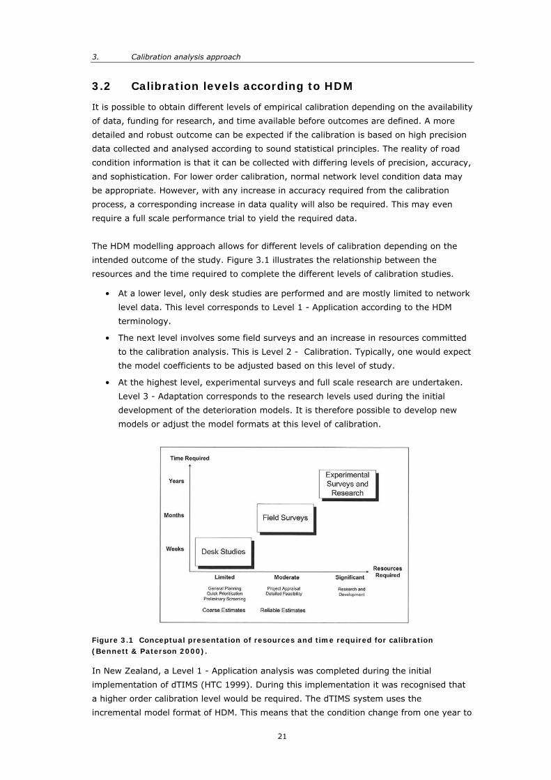
The HDM modelling approach allows for different levels of calibration depending on the
intended outcome of the study. Figure 3.1 illustrates the relationship between the
resources and the time required to complete the different levels of calibration studies.
• At a lower level, only desk studies are performed and are mostly limited to network
level data. This level corresponds to Level 1 - Application according to the HDM
terminology.
• The next level involves some field surveys and an increase in resources committed
to the calibration analysis. This is Level 2 - Calibration. Typically, one would expect
the model coefficients to be adjusted based on this level of study.
• At the highest level, experimental surveys and full scale research are undertaken.
Level 3 - Adaptation corresponds to the research levels used during the initial
development of the deterioration models. It is therefore possible to develop new
models or adjust the model formats at this level of calibration.
Figure 3.1 Conceptual presentation of resources and time required for calibration (Bennett & Paterson 2000).
In New Zealand, a Level 1 - Application analysis was completed during the initial
implementation of dTIMS (HTC 1999). During this implementation it was recognised that
a higher order calibration level would be required. The dTIMS system uses the
incremental model format of HDM. This means that the condition change from one year to

A REVIEW OF THE HDM/DTIMS PAVEMENT MODELS BASED ON CALIBRATION SITE DATA
22
another is forecast. Calibrating the incremental model therefore requires robust condition
data, as the expected condition change from one year to another is relatively small. The
objective for the New Zealand calibration programmes was to collect the condition data to
satisfy Level 3 – Adaptation. The intention was to be able to perform a Level 2 calibration
within the shortest time-frame. Later, with sufficient data becoming available, a Level 3
calibration becomes possible, as explained in this study.
While the layout of the experiment and the development of the condition survey
specifications are an integral part of the study, this will not be documented in detail as
part of this report. For further information on the data collection, a copy of Henning et al.
(2004b) is provided in Appendix A.
3.3 Analysis approach for HDM calibration Level 2
The main objective for Level 2 calibration is to adjust the calibration coefficients. The
following sections provide experience and best practice regarding the calibration of the
different pavement deterioration models.
3.3.1 Crack initiation
3.3.1.1 Existing model format
The HDM-4 crack initiation model forms are separated firstly for stabilised and granular
bases and secondly for original surfacing and resurfacing of existing surfaces. Most
New Zealand roads fall within the granular base category because most pavements are
only lightly stabilised compared to world practice. The crack initiation for these types of
pavements is (NDLI 1995): Original Surfaces:
⎭⎬⎫
⎩⎨⎧
+⎥⎦
⎤⎢⎣
⎡⎟⎠⎞
⎜⎝⎛+= CRTSNPYE4aSNPaexpaCDSKICA 2210
2cia
(Equation 3.1)
Resurfaced Surfaces:
⎪⎪
⎭
⎪⎪
⎬
⎫
⎪⎪
⎩
⎪⎪
⎨
⎧
+
⎥⎥⎥⎥⎥
⎦
⎤
⎢⎢⎢⎢⎢
⎣
⎡
⎟⎟⎟⎟⎟
⎠
⎞
⎜⎜⎜⎜⎜
⎝
⎛
⎟⎟⎠
⎞⎜⎜⎝
⎛
⎥⎦
⎤⎢⎣
⎡⎟⎠⎞
⎜⎝⎛+
= CRTHSNEWao,
aPCRW-1MAX
*SNPYE4aSNPaexpa
MAXCDSKICA
43
22102
cia (Equation 3.2)
where:
ICA time to initiation of ALL structural cracks (years)
CDS construction defects indicator for bituminous surfaces
YE4 annual number of equivalent standard axles (millions/lane)
SNP average annual adjusted structural number of the pavement
HSNEW thickness of the most recent surface (mm)
PCRW area of all cracking before latest reseal or overlay (% of total cracking
area)

3. Calibration analysis approach
23
Kcia calibration factor for initiation of all structural cracking
CRT crack retardation time because of maintenance (years)
ai model coefficients
The expressions basically consist of a structural crack component which is dependent on
the SNP and the YE4/SNP2. This value is then multiplied by the previous cracking and
thickness of a new surface, for resurfaced sections.
3.3.1.2 Crack initiation calibration methodology
The HDM proposed method to calibrate crack initiation models is (Bennett & Paterson
2000):
PTCImeanOTCImean Kci = (Equation 3.3)
where the ( )[ ]{ } PTCI - OTCImeanSQRT RMSE n1,j2
jj ==
RMSE root means square error is the error function to minimise
OTCI observed time to crack initiation
PTCI predicted time to crack initiation
The disadvantage of the HDM approach is that it takes account only of sections that are
cracked, thus ignoring sections which outlast expected performance. This method will
therefore be biased towards early cracked sections. In order to take account of sections
that are un-cracked beyond the point of predicted cracking, Jooste proposed an
alternative method as documented in Rohde et al. (1998).
According to this method, Kci is determined according to an iterative process which
minimises the error (Err) between the predicted and the actual crack initiation process.
The error is calculated according to Rohde et al. (1998):
( )∑ −= 22i SAGETYCRwErr (Equation 3.4)
where:
Err is the error function to be minimised over the number of sections
SAGE2 is the actual seal age at the time when crack initiation took place (first
observation of cracking) or the current age when the section is still
uncracked;
TYCR is the predicted time to crack initiation
wi is the weighting factors:
0.0 if TYCR > SAGE2 and the pavement is uncracked
1.0 if TYCR < SAGE2 and the pavement is uncracked
1.5 if TYCR < SAGE2 and the pavement is cracked
1.0 if TYCR > SAGE2 and the pavement is cracked
The above weightings were subjectively derived and tested according to the model
prediction outcome. According to outputs presented later in this report, the weightings
are seen to be working well for New Zealand conditions.

A REVIEW OF THE HDM/DTIMS PAVEMENT MODELS BASED ON CALIBRATION SITE DATA
24
Note that the differences between the RMSE and the Err error functions are:
• RMSE is expressed in terms of predicted and actual crack initiation. The Err
function also incorporates surface age for pavements that have not cracked yet.
• The RMSE is calculated by taking the mean and square root of the difference
between the predicted and actual crack initiation. The Err only takes the power of
the difference, but it includes a weighting factor which is not included in the
RMSE.
3.3.2 Crack progression models
The HDM crack progression model has a sigmoidal format. It is normally problematic to
calibrate these since it takes a long time to collect these data in an experiment, and crack
progression is seldom found on a network given early maintenance intervention. For this
reason the HDM guidelines (Bennett & Paterson 2000) recommend a simple approach of:
cicp K
1 K = (Equation 3.5)
where: Kcp is the calibration coefficient for crack progression
Kci is the calibration coefficient for crack initiation
For instances where crack progression data are available, the following method could be
used:
ET30meanPT30mean K cp = (Equation 3.6)
where:
PT30 is the predicted age at 30% cracking
ET30 is the actual age at 30% cracking
According to previous attempts, the calibration of the crack progression model is difficult.
Firstly, no historical data are kept after cracks have been sealed. Secondly, cracked
sealed quantities are often not kept. However, the crack progression model has a low
priority since engineering experience has indicated that the actual crack quantity is not
very significant compared to the simple information of when a pavement cracks (i.e. crack
initiation). This fact has been confirmed in some of the results in this report (see
Section 4.2.2). For this reason, the crack progression model will not be investigated in
this report.
3.3.3 Rut progression
3.3.3.1 Model description
The HDM-4 rutting model consists of the following components:
• initial densification,
• structural deformation,
• plastic deformation,
• wear from studded tyres.

3. Calibration analysis approach
25
Only the first three components of the rut progression are relevant to New Zealand
conditions as studded tyres are not used in New Zealand. The following paragraphs
discuss the model formats in more detail.
3.3.3.2 Initial densification
The initial densification is given by (NDLI 1995):
( )( )[ ]4321 aaDEFaa60rid COMPSNPYE410aKRDO +
= (Equation 3.7)
where:
RDO is the rutting caused by initial densification (mm)
Krid calibration coefficient for initial densification
YE4 annual number of equivalent standard axles (millions/lane)
DEF average annual Benkelman Beam deflection (mm)
SNP adjusted structural number of the pavement
COMP relative compaction (%)
ai model coefficients The initial densification phase for rutting is valid for New Zealand conditions. Of specific
interest is the relationship between the initial rut progression and the standard deviation.
Currently, HDM-4 provides a positive linear relationship between rutting and the resulting
rut depth standard deviation. It is believed that this trend may be negative during the
initial stages of densification. The rut depth standard deviation is further discussed in
Section 6.4.
3.3.3.3 Structural deformation
It is recognised by engineers that rutting is a very good indicator of the structural health
of a pavement. For example, rutting is one of the key performance indices used on
performance-specified maintenance contracts. Koniditsiotis & Kumar (2004) have
demonstrated how to utilise the shape of the transverse profile in order to predict
pavement structural capacity. The authors have establish a remarkable correlation
between the rut patterns and pavement strength/capacity. It is anticipated that the
rutting performance on networks will become more important in future as the
understanding of this condition indicator increases.
HDM-4 provides two forms of rutting progression for cracked and un-cracked sections
(NDLI 1995):
• Structural deformation for un-cracked sections
( )a3a2a1
0rstUC COMPYE4SNPaKΔRDST = (Equation 3.8)

A REVIEW OF THE HDM/DTIMS PAVEMENT MODELS BASED ON CALIBRATION SITE DATA
26
• Structural deformation after cracking
( )a4a3a2a1
0rstcrk ACXMMPYE4SNPaKΔRDST = (Equation 3.9)
where
∆RDST is the incremental increase in structural deformation in the analysis year
(mm)
Krst calibration coefficient for structural deformation
YE4 annual number of equivalent standard axles (millions/lane)
COMP relative compaction (%)
MMP mean monthly precipitation (mm/month)
SNP adjusted structural number of the pavement
ACX area of indexed cracking (% of total carriageway area)
ai model coefficients
3.3.3.4 Plastic deformation
The HDM-4 plastic deformation is presented as (NDLI 1995):
a2a10
3rpd HSYE4ShaCDSKΔRDPD= (Equation 3.10)
where:
∆RDPD is the incremental increase in plastic deformation in the analysis year
(mm)
Krpd calibration coefficient for plastic deformation
CDS construction defects indicator
YE4 annual number of equivalent standard axles (millions/lane)
Sh speed of heavy vehicles (km/h)
HS total thickness of the bitumen surface
ai model coefficients
Default model coefficients are provided for both asphalt and chipseal pavements. The
model format and the coefficients have to be validated for New Zealand roads, which
often consist of multiple-surfaced layers.
3.3.4 Rutting calibration methodology
The calibration of the rut progression is a simple process of comparing the predicted with
the actual rut depths:
Calculate the adjustment factor for mean rut depth progression, by geometric means or
from log values (logORDMj and logPRDMj) as follows (Bennett & Paterson 2000):
PRDMj)] [Sum(log / ORDMj)] (log [Sum Kor [PRDMj] MeanGeometric / [ORDMj] MeanGeometric K
rp
rp
=
= (Equations 3.11, 3.12)
where
Krp is the rut depth progression calibration coefficient
PRDMj is the predicted rut depth for section

3. Calibration analysis approach
27
ORDM is the observed rut depth The rut depth standard deviation is calibrated according to the same principle.
3.3.5 Surface texture
The classical HDM format of the texture depth model incorporated a complex process of
combining two stages in the loss of texture depth (Figure 3.2). The initial stage sees a
rapid loss in texture depth caused by the re-orientation and embedment of the seal chips.
This stage is followed by a very slow loss in texture depth caused by the interaction
between the surface and the vehicle tyres. The application of the texture depth model is
difficult, given the sensitivity of the model towards the intercept point between the rapid
texture loss phase and the gradual loss of texture later during the surface life. The main
disadvantage of the model was the sensitivity to the reset (works effect) setting following
construction. For example, if the wrong texture depth was assigned following
construction, the error was compounded by the steep gradient for the initial texture loss
according to HDM.
For this reason Transit (2003) conducted a study to determine a simplified method of
calibrating the texture depth model. This was achieved by assuming a simplified model
format as illustrated in Figure 3.2. Therefore, only the texture loss slope is derived and
applied to the current texture value. For new work, a default texture depth at year one or
two is assumed.
Initial Stage Slow Texture Loss
Original HDMModel Format
SimplifiedModel Format
Time
Mea
n Te
xtur
eD
epth
Figure 3.2 Changes to texture depth model format.
The proposed model calibration methodology included an option of three different
methods Transit (2003):
• Method 1 - Section Calibration of Texture Coefficients using the current HDM
incremental texture model;
• Method 2 - National Calibration of Texture Coefficients using the current HDM
incremental texture model; and

A REVIEW OF THE HDM/DTIMS PAVEMENT MODELS BASED ON CALIBRATION SITE DATA
28
• Method 3 – Regional Calibration of Texture performance using developed
Surface Age texture model.
Method 1 involves analysing section specific data as illustrated in Figure 3.3.
The details for the calculation of the calibration coefficients are as follows (Transit 2003):
)Y1(YLog
)t(tkkn
n10
1nn21 += + (Equation 3.13)
where:
tn, tn+1 is texture depth at year Yn and Yn+1 and tn>tn+1
Y(n, n+1) is the surface age at date of texture reading ((reading date – surface
date)/365)
kt1kt2 is texture deterioration slope
(NELV) logktkt t kt 1021n1 += (Equation 3.14)
where:
NELV = {365.Yn[(1-f)AADT+10fAADT]}
f = fraction of HCVs
kt2 = kt1kt2/kt1
2.0
2.1
2.2
2.3
2.4
2.5
2.6
2.7
3 4 5 6 7 8 9 10
Surface Age (Years)
Ave
rage
Mea
n Pr
ofile
Dep
th (m
m)
Measured MPD on Treatment Length Basis for Texture Calibration
Figure 3.3 Method 1 section calibration principle (treatment length) (Transit 2003).
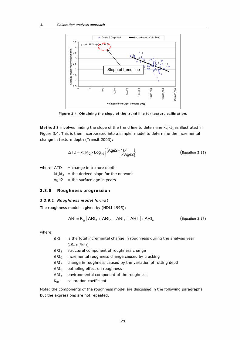
Method 2 involves the analysis of a full network or regional analysis to yield the
calibration coefficients for the HDM texture depth model. It follows a similar process to
Method 1, with the exception that kt1kt2 (regression slope) is determined by performing a
regression analysis on the texture depth and equivalent light vehicles (Figure 3.4). Once
kt1kt2 is determined, the equations for Method 1 are used to determine kt1 and kt2.
3. Calibration analysis approach
29
y = -0.181 * Ln(x) + 4.9430
0.5
1
1.5
2
2.5
3
3.5
4
4.5
1 10 100
1,00
0
10,0
00
100,
000
1,00
0,00
0
10,0
00,0
00
100,
000,
000
Net Equivalent Light Vehicles (log)
Ave
rage
Mea
n Pr
ofile
Dep
th (m
m)
Grade 2 Chip Seal Log. (Grade 2 Chip Seal)
Figure 3.4 Obtaining the slope of the trend line for texture calibration.
Method 3 involves finding the slope of the trend line to determine kt1kt2 as illustrated in
Figure 3.4. This is then incorporated into a simpler model to determine the incremental
change in texture depth (Transit 2003):
( )⎭⎬⎫
⎩⎨⎧ +×= Age2
1Age2LogktktΔTD 1021 (Equation 3.15)
where: ∆TD = change in texture depth
kt1kt2 = the derived slope for the network
Age2 = the surface age in years
3.3.6 Roughness progression
3.3.6.1 Roughness model format
The roughness model is given by (NDLI 1995):
[ ] etRCSgp ΔRIΔRIΔRIΔRIΔRIKΔRI ++++= (Equation 3.16)
where:
∆RI is the total incremental change in roughness during the analysis year
(IRI m/km)
∆RIS structural component of roughness change
∆RIC incremental roughness change caused by cracking
∆RIR change in roughness caused by the variation of rutting depth
∆RIt potholing effect on roughness
∆RIe environmental component of the roughness
Kgp calibration coefficient
Note: the components of the roughness model are discussed in the following paragraphs
but the expressions are not repeated.
Slope of trend line

A REVIEW OF THE HDM/DTIMS PAVEMENT MODELS BASED ON CALIBRATION SITE DATA
30
In the New Zealand context the potholing and cracking components of the roughness
model can be ignored. New Zealand engineers follow an intensive routine maintenance
regime so that these two parameters do not affect the roughness significantly.
3.3.7 Roughness model calibration
The roughness model consists of two calibration factors, namely Kge (an environmental
calibration coefficient) and Kgp (the calibration coefficient that caters for roughness
increase caused by traffic loading).
The recommended calibration procedure for the roughness model is summarised below.
3.3.7.1 Adjustment of the environmental coefficient
According to Bennett & Paterson (2000), Kge and Kgp seldom need adjustment once the
environmental coefficient m is established. The guides recommend a slice-in-time2
analysis for adjustment of the environmental coefficient, inverting the absolute models of
Paterson & Attoh-Okine (1992):
[ ]
3AGE)SNP1(
4NE135RIlnAPAT056.0ACRX0068.0RDS143.0RI02.1lnm
5t
0tttt ⎥⎦
⎤⎢⎣
⎡
++−−−−
= (Equation 3.17)
[ ]
3AGE)SNP1(4NE263RIlnRIln
m5t
0t ⎥⎦
⎤⎢⎣
⎡
++−
= (Equation 3.18)
where:
RIt = roughness at AGE3 years after construction
RI0 = roughness when new
NE4t = cumulative axle loading since construction
RDSt = standard deviation of rut depth at AGE3
ACRXt = area of indexed cracking at AGE3
APATt = area of patching at AGE3
This method is not always effective since it strongly relies on the correct estimation of
RI0. If it is based on actual data, it is often found that the scatter in RI0 ranges more than
the actual increase of roughness over time. Experience in New Zealand suggested that
this method does not yield satisfactory results (Hallett & Tapper 2000).
3.3.7.2 Adjustment of all model coefficients – Riley’s method
Riley proposed an alternative calibration analysis process for the roughness model in
Henning & Riley (2000). An extract from this method is provided below:
2 Slice-in time method takes the performance of pavements at a current date. The predicted value
(for the given age) is compared with the performance of the pavement since its construction to the current age.

3. Calibration analysis approach
31
The following steps should be carried out in a spreadsheet.
Step 1
Obtain the best estimate of the environmental variable (m).
Step 2
Calculate the mean incremental values of IRI and RDS. In Excel the SLOPE
function is useful for this purpose.
Step 3
Calculate the mean absolute values of IRI.
Step 4
Calculate the predicted values of the structural term using SNC, axle loading,
construction age and the initial estimate of m from Step 1:
5SNC)(1YE4AGE3)exp(m
term Structural+
=
Step 5
Make a multiple linear regression of observed mean incremental IRI against
the following terms:
predicted structural component of roughness increment from Step 4
observed mean increment in RDS from Step 2
observed mean absolute value of IRI from Step 3
The intercept should be set to zero when carrying out the regression.
The regression coefficients will then give a modified version of the component
incremental model:
a5 IRI3aRDS2a)SNC1(
4YE)3AGEmexp(1aIRI +++
=
If the derived value of m (regression coefficient a3) differs significantly from
the value obtained in step 1, repeat steps 4 and 5 using the value a3. Repeat
the process until a stable value of m is obtained.
It is thought that the above method will be appropriate for rural roads where
a time series of high speed data is available. However, many RCAs may have
a time series of roughness data but lack data on RDS, having only RAMM
data (length with rutting > 20 mm or 30 mm). It is thought that RDS is a
major influence on roughness.

A REVIEW OF THE HDM/DTIMS PAVEMENT MODELS BASED ON CALIBRATION SITE DATA
32
In urban areas, the area of patching may be a significant roughness
component. If a historical time series of patched areas (whether pavement
repairs or utility cuts) is available the mean incremental patching should be
included as an additional term in the regression described above.
3.3.8 Pothole initiation and progression
Pothole initiation is fixed based on the cracking and ravelling initiation and progression.
Only the progression can be calibrated according to Bennett & Paterson (2000):
For each calibration section, estimate the time for initiation of cracking
(PTCI), the time for initiation of potholing (PTPI), and the time for
progression of potholing to X units (PTPX) up to 500 potholing units.
Compute the observed and predicted potholing times as follows:
PTPIj - AGESOTPXj =
PTPIj - PTPXj PTPXj =
Determine the potholing adjustment factor, either by linear regression of
OTPXj against PTPXj, or as follows:
( )( )
PTPXjmean
OTPXjmean Kph =
Calibrating potholing in New Zealand would not be possible. Even on the calibration
sections, potholes are not allowed because of safety concerns to the user. For that
reason, the default model settings are accepted for pothole prediction.
3.4 Analysis approach for HDM calibration level 3 – Adaptation
Level 3 – Adaptation analysis could include either of the following approaches:
Adjusting current base HDM model format. The HDM base models are provided with
a number of coefficients in addition to the calibration coefficients. These coefficients are
provided to make provision for different material types, construction methods and soil
conditions. They provide significant flexibility to the model calibration process. In Transit
(2004) it was demonstrated that the correlation of the crack initiation model is greatly
improved by adjusting these coefficients.
Developing new models based on first principles. Should it be established that a
particular model format is inappropriate for the area in which it is applied, a new model
format needs to be established. It is recommended that a similar approach be followed to
the original HDM models as follows (adapted from Bennett & Paterson 2000):
3. Calibration analysis approach
33
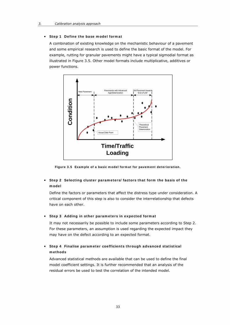
• Step 1 Define the base model format
A combination of existing knowledge on the mechanistic behaviour of a pavement
and some empirical research is used to define the basic format of the model. For
example, rutting for granular pavements might have a typical sigmodial format as
illustrated in Figure 3.5. Other model formats include multiplicative, additives or
power functions.
C
ondi
tion
Time/TrafficLoading
New Pavement Pavements with AdvancedAge/Deterioration
Old Pavement towards‘End of Life”
Actual Data Point
TheoreticalPavementDeterioration
Figure 3.5 Example of a basic model format for pavement deterioration.
• Step 2 Selecting cluster parameters/factors that form the basis of the
model
Define the factors or parameters that affect the distress type under consideration. A
critical component of this step is also to consider the interrelationship that defects
have on each other.
• Step 3 Adding in other parameters in expected format
It may not necessarily be possible to include some parameters according to Step 2.
For these parameters, an assumption is used regarding the expected impact they
may have on the defect according to an expected format.
• Step 4 Finalise parameter coefficients through advanced statistical
methods
Advanced statistical methods are available that can be used to define the final
model coefficient settings. It is further recommended that an analysis of the
residual errors be used to test the correlation of the intended model.

A REVIEW OF THE HDM/DTIMS PAVEMENT MODELS BASED ON CALIBRATION SITE DATA
34
4. Crack initiation
4.1 HDM level 2 calibration
4.1.1 Cracking data used for the level 2 calibration
Given that the LTPP data have only been collected for the past three years, the data were
not statistically robust for crack initiation calibration. An opportunity existed, however, to
utilise the network survey data collected on the LTPP sections for this purpose. Most of
the Transit LTPP sections are contained within the Transit benchmark sections. These
benchmark sections are 1 km-long sections that undergo repetitive High Speed Data
(HSD) surveys on an annual basis, and the visual rating is undertaken on these sites
according to the RAMM survey methods. The repetitive HSD data are then used to
benchmark the network HSD surveys in order to identify any bias in the equipment during
the surveys. Since comprehensive inventory and condition data (RAMM rating) were
available on these sections dating back as far as 1999, it was possible to perform the
crack calibration using the benchmark section data.
Historical crack records from the RAMM rating data were interpreted according to
Figure 4.1. Note that the inspection length of the rating was not always consistent since
the start/end may have shifted over the years. However, it was aimed at using only the
data points within the boundaries of the benchmark section.3 Also note that the survey of
the entire benchmark section length started in 2001.
1 Km Benchmark Length
300m Calibration Length (LTPP)
Distance
Tim
e (Y
ears
)
1995
2001
2002
Resurface Date
PCA (%Cracking Before Resurface)
Cracking observed for the first time
Time to Crack Initiation (TYCR)
Inspection Lengths
Figure 4.1 Interpretation of cracking data (Transit 2004).
3 The time to crack initiation was defined as the first observation in time when the crack
percentage exceeded 0.5% of the total benchmark pavement area or the area of the rated section if it was shorter than the benchmark section.

4. Crack initiation
35
4.1.2 Results
The resulting regional calibration factors are presented in Table 4.1 and Figure 4.2. The
Transit LTPP sections are located in four climatic regions as described in Henning et al.
(2004b), according to a climatic classification method proposed by Cenek (2001).
According to this method, the climatic regions are classified according to the ratio of
rainfall:wet strength properties of the soil. High and moderate risk areas include wetter
areas combined with more sensitive soil areas (e.g. Northland), whereas low and limited
risk areas are the drier and more stable soil types such as Canterbury. Statistically, more
than 15 sections in each sub-category are required in order to have sufficient data for
meaningful results. Sufficient data were available to group the results into only two
climatic regions in order to obtain statistically significant results. The table indicates a
smaller crack initiation factor (Kci) for the high and moderate risk areas, thus suggesting
an earlier crack initiation period. This observation is consistent with expectations, and
also confirms the validity of the climatic regions as adopted for this study. The New
Zealand outcome (Kci equals approximately 0.5) compares well with other international
calibration results (Rohde et al. 2002). Furthermore, New Zealand heavy rainfall and clay-
type materials are expected to give a calibration coefficient which is less than 1.
Table 4.1 Summary of calibration result for different climatic regions (Transit 2004).
Factor Regional Classification
High and Moderate Low and Limited
Kci 0.49 (0.52) 0.59 (0.64)
Error(Err) – Default 194 477
Error(Err) – Calibrated
27 160
Notes: The error is calculated according to Section 3.3.1. The values in brackets are the calibration coefficients obtained from data explained in
Section 4.2.1.
Figure 4.2 illustrates the comparison between observed and predicted crack initiation. It
further classifies the data according to four categories that indicate the relationship
between predicted and actual crack initiation time. An observation from this figure is that
the range of predicted crack initiation is much narrower compared with the range in
actual crack initiation time. This observation corresponds well with calibration results
obtained elsewhere (Henning et al. 1998). The wider spread in actual crack initiation time
compared to the model can be explained as follows:
• A wider range will always be recorded in observed than predicted values because of
the natural spread of the actual data and influences from external factors which are
not incorporated into the model.
• The model calibration outcome as presented in this section involved only the
adjustment of the climatic calibration coefficient. A closer fit between the actual and
the predicted crack initiation can be obtained by adjusting all the model
coefficients.
• different crack mechanisms may possibly exist, and aggregating them into one
single analysis produces a poorer fit between the actual and predicted observations.

A REVIEW OF THE HDM/DTIMS PAVEMENT MODELS BASED ON CALIBRATION SITE DATA
36
The latter two points relate to model form definitions and will be discussed further in this
chapter.
Cracking Initiation (Calibrated)
02468
10121416
0 2 4 6 8 10 12 14 16
Predicted Initiation Time
Obs
erve
d In
itiat
ion
Tim
e
Cracked Earlier than Predicted Cracked Later Than PredictedPredicted Cracked Still Uncracked Predicted Uncracked Still Uncracked
Line of Equality
Notes: Data included for all Benchmark Sections that correspond with the LTPP sections (i.e. 40
sections across New Zealand). When calculating the predicted initiation time, the SNP was based on the back analysis of the average FWD reading for each section. Results represent a default HDM-III crack initiation model.
Figure 4.2 Comparing actual cracking with predicted cracking (Transit 2004).
4.2 A review of the cracking model format
4.2.1 Crack initiation data for the model review
As illustrated in Section 4.1.1, the crack initiation data are limited for the Transit LTPP
sections and benchmark sections. In order to expand the crack initiation data, network
RAMM survey data were considered and found to be appropriate. The RAMM rating
consists of assessing the length of cracked wheel path. This length of cracking is
subsequently converted to percentage cracking, according to conversion factors
documented in HTC (1999):
hinsp_lengt
50Alligator0.28
2
hinsp_lengt
50xAlligator0.0004 Cracking Percentage += ⎟
⎠⎞
⎜⎝⎛ (Equation 4.1)
where:
Percentage Cracking is percentage of the total lane area cracked
Alligator length (m) of the wheel path showing alligator cracking
insp_length inspection length in (m) The accuracy of this conversion does not cause any concern, since the crack initiation is
identified at a point when the cracking exceeds 0.5% (or an equivalent of approximately
2 m of cracking on a 50-m rating section), and the accuracy is therefore not too sensitive
to the outcome. It was important though, to select appropriate rating sections for the
analysis in order to ensure that the same 50-m rating section was assessed for a number
of years.

4. Crack initiation
37
Two Transit regions (East Wanganui and Coastal Otago) were selected for the crack
analysis. These two regions represent pavement deterioration for a medium and low
climatic sensitivity area respectively (see Henning et al. 2004b). Furthermore, the data
availability and knowledge of these networks allowed for an in-depth data interrogation.
Specific sections used for the analysis were extracted according to the following criteria:
• Sections were included where the location of the 50-m rating sections have not
changed from survey to survey.
• Each section had a minimum of four rating years.
• All information was extracted for comparing before-and-after performance of
resurfacing (cracking in particular).
Only chipseal pavements were analysed for the purposes of the model development. Once
the model format has been reviewed, further analysis will also be completed on
alternative surface types. The data were also categorised for sections that had more than
three layers of surfaces, and whether they were cracked before resurfacing. The
distribution from the cracking data for the respective regions is presented in Figure 4.3.
East Wanganui
Time to Crack Initiation
Num
ber o
f Obs
erva
tions
2 4 6 8 10 12 14
05
1015
2025
Coastal Otago
Time to Crack Initiation
Num
ber o
f Obs
erva
tions
5 10 15
010
2030
40
Note difference in scale Figure 4.3 Distribution of crack initiation for the two regions.
As expected, the average time to crack initiation was longer on the Coastal Otago region,
thus confirming the appropriateness of the climatic classification. Coastal Otago consists
of more stable soils and climatic conditions. It is also observed that more data were
extracted from the Coastal Otago region, since the rating sections for this region were
more stable over time. The imbalance of the data between the two regions was
considered in the analysis.

A REVIEW OF THE HDM/DTIMS PAVEMENT MODELS BASED ON CALIBRATION SITE DATA
38
4.2.2 Refining the existing HDM model format
In the 2004 Transit study two methods were shown to be available to improve the crack
initiation model:
• accept the HDM model format, but adjust all the model coefficients based on local
data,
• a full review of the model that includes multivariate and regression analysis.
Both these methods were used and the adjustment of the HDM model coefficients is
described in this section. Model coefficients a0 to a4 were adjusted by minimising the error
between the predicted and the observed crack initiation (see Section 3.1.3). Note that
both the cracked and uncracked sections were considered during this analysis.
Table 4.2 Resulting model coefficients for existing HDM model format.
Default HDM crack initiation model HDM crack initiation model with adjusted coefficients
a0 a1 a2 a3 a4
13.2 0 20.7 20 0.22
a0 a1 a2 a3 a4
8.3 0 18.54 0.01 0.34
Cracking Initiation (Un-Calibrated)
02468
10121416
0 2 4 6 8 10 12 14
Predicted Initiation Time
Obs
erve
d In
itiat
ion
Tim
e
Cracked Earlier than Predicted Cracked Later Than Predicted
Error = 17597.7
Cracking Initiation (Calibrated)
02468
10121416
0 2 4 6 8 10 12 14
Predicted Initiation Time
Obs
erve
d In
itiat
ion
Tim
e
Cracked Earlier than Predicted Cracked Later Than Predicted
Error = 6697.9
Note: For the purpose of clarity, sections with no cracking observed are not indicated on the graphs.
Observations from Table 4.2 include:
• Using the new coefficients has reduced the error significantly from 17,597 to 6,697.
• Uncalibrated, the predicted crack initiation ranged from 1 to 13 years compared to
the actual 1 to 16 years. The corresponding range for the predicted cracking
initiation using refined coefficients ranged from 1 to just over 8 years. The current
model and/or calibration process has limitations since the outcome gives a better fit
for the over-all model, but does not necessary reflect the reality (e.g. the actual
maximum is 16 years).
• The uncalibrated model does not predict any crack initiation over 13 years, and the
maximum time to crack initiation for the calibrated model is just over 8 years.
• Most of the predicted crack initiation periods are between 10 and 13 years, and
between 6 and 8 years for the default and calibrated model respectively.

4. Crack initiation
39
Changes to the model coefficients suggest that cracking initiation caused by the
loading/strength relation YE4/SNP2 is reduced (both a0 and a2 have reduced). The
influence of the new surface thickness has increased (a4 increased). The influence of
percentage cracking before resurfacing has changed completely. The coefficient a4 has
changed from a value of 20 to a significantly smaller number (0.01). For the default
model, the ratio between the previous cracking and the coefficient was a continuous
variable, whereas the calibrated model suggested that it is a binary variable (either 0 or
1). This suggests that crack initiation is a function of whether the old surface consisted of
previous cracking or not. The actual value of previous cracking is not significant. Although the calibrated model has a significantly better fit to the actual crack initiation, it
is observed that the scatter between predicted and observed crack initiation time is still
significant. Having looked at the figures in Table 4.2, one has to conclude that the model
has little 'prediction power'.
4.2.3 Variable analysis
New model form development can be divided into three stages as follows:
• Variable analysis is aimed at better understanding the relationships between the
possible variables and the predicted variable. During this stage it is also important
to search for any inter-variable relationships. General trends and possible relation
forms are noted during this phase, since it could simplify regression analysis which
follows later.
• Subsequently multi-variate analysis is undertaken to determine the significant
variables that influence the independent variable.
• Last, the regression is undertaken to define in which format the variables are
combined, in order to predict the outcome of the independent variable.
Table 4.3 shows the variables considered during the analysis in the following sections.
Table 4.3 Variables considered for predicting crack initiation.
Variable Description Variable Type
AADT the annual average daily traffic Continuous
YE4 annual number of equivalent standard axles (millions/lane)
Continuous
SNP Structural Number of the Pavement Continuous
Surf_Gen generation of the surface (for example first generation surfaces would be equal to 0 and represent the original surface layer after construction, and 1 representing all subsequent surfaces)
Factor
CS_PCA cracked status before resurfacing (0 or 1 for uncracked or cracked)
Factor
HTOT total surface thickness (mm) of all the layers Continuous
HNEW surface thickness (mm) of the latest surfaced layer Continuous
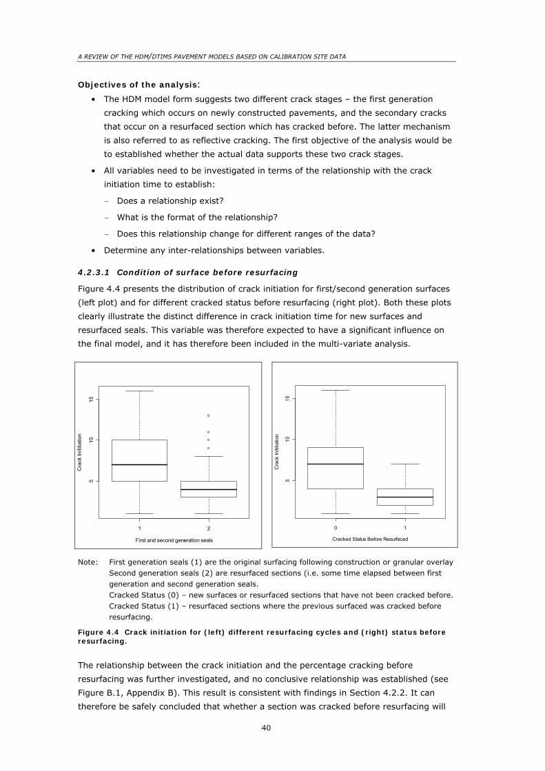
A REVIEW OF THE HDM/DTIMS PAVEMENT MODELS BASED ON CALIBRATION SITE DATA
40
Objectives of the analysis: • The HDM model form suggests two different crack stages – the first generation
cracking which occurs on newly constructed pavements, and the secondary cracks
that occur on a resurfaced section which has cracked before. The latter mechanism
is also referred to as reflective cracking. The first objective of the analysis would be
to established whether the actual data supports these two crack stages.
• All variables need to be investigated in terms of the relationship with the crack
initiation time to establish:
- Does a relationship exist?
- What is the format of the relationship?
- Does this relationship change for different ranges of the data?
• Determine any inter-relationships between variables.
4.2.3.1 Condition of surface before resurfacing
Figure 4.4 presents the distribution of crack initiation for first/second generation surfaces
(left plot) and for different cracked status before resurfacing (right plot). Both these plots
clearly illustrate the distinct difference in crack initiation time for new surfaces and
resurfaced seals. This variable was therefore expected to have a significant influence on
the final model, and it has therefore been included in the multi-variate analysis.
1 2
510
15
First and second generation seals
Cra
ck In
ititia
tion
0 1
510
15
Cracked Status Before Resurfaced
Cra
ck In
ititia
tion
Note: First generation seals (1) are the original surfacing following construction or granular overlay Second generation seals (2) are resurfaced sections (i.e. some time elapsed between first generation and second generation seals. Cracked Status (0) – new surfaces or resurfaced sections that have not been cracked before. Cracked Status (1) – resurfaced sections where the previous surfaced was cracked before resurfacing.
Figure 4.4 Crack initiation for (left) different resurfacing cycles and (right) status before resurfacing.
The relationship between the crack initiation and the percentage cracking before
resurfacing was further investigated, and no conclusive relationship was established (see
Figure B.1, Appendix B). This result is consistent with findings in Section 4.2.2. It can
therefore be safely concluded that whether a section was cracked before resurfacing will

4. Crack initiation
41
have a significant influence on the crack initiation period. However, the actual crack
percentage before resurfacing is not significant.
It remains questionable whether both these variables should be included in the model.
One of the aims of this process is to keep the final model as simple as possible, which
may result in only one of these two variables being used.
4.2.3.2 Thickness of the new surface and the total surface thickness
Figure 4.5 shows the relationship between surface thickness and crack initiation. Two
thicknesses were considered:,
• the new surface thickness,
• the total surface thickness.
No apparent relationship exists between the new surface thickness and the crack initiation
time. Note, however, that the new surface thickness was derived from an assumed
thickness given the surface code in RAMM. From experience, these data are not always
accurate. Furthermore, the thickness does not indicate the film thickness of the bitumen
in the surface. The film thickness of the bitumen is the inferred variable adopted in the
HDM model. Oliver (2004) has demonstrated the significance of the bitumen age and
thickness on the crack initiation period. However, this relationship was not confirmed with
the data from the State Highway RAMM database.
Figure 4.5 (right-hand plot) shows an apparent exponential relationship between the total
thickness and the crack initiation period. Possible explanations for this observed trend
are:
• Multiple surface layers indicate older pavements which are more prone to cracking
or were cracked before the last resurfacing. Cracking observed on these sections is
therefore reflective cracking of third, fourth or even later generation seals.
• Multiple surface layers are well known to be more unstable (HTC 1999). Significant
movement and flexing of the surface layers can therefore be assumed to occur,
thus resulting in more strains and subsequent cracking of the newly surfaced layer.
Uncertainty still exists as to whether the total surface thickness should be included as a
continuous variable, or whether thickness should be categorised into different levels. This
aspect is further investigated in Section 4.2.5.

A REVIEW OF THE HDM/DTIMS PAVEMENT MODELS BASED ON CALIBRATION SITE DATA
42
5 8 10 12
510
15
Thickness of new surface
Tim
e to
cra
ck in
itiat
ion
5 15 22 27 30 34 40 49 52 64 112
510
15
total thickness of surface
Cra
ck In
ititia
tion
Figure 4.5 Relationship between (left) thickness of new surface and (right) total surface thickness with the crack initiation period.
4.2.3.3 Pavement strength (SNP)
The relationship between the crack initiation and structural number (as an isolated
variable) was investigated, and no apparent relationship was observed. Figure 4.6
illustrates the crack initiation as a function of structural number. The figure shows the
same relation, but for different surface thicknesses and cracked status. No sensible
relation was observed in any of the graphs depicted in Appendix B.
510
15
0 1 2 3 4 5 6
0 1 2 3 4 5 6
510
15
Structural Number
Cra
ck In
ititia
tion
0
1
Given : Thin -1 or Thick-2
0
1
Giv
en :
Sta
tus
of C
rack
ing
befo
re R
esur
face
(0-n
o cr
acks
)
Figure 4.6 Crack initiation as a function of structural number for different combinations of surface thickness and cracked status.
The lack of a relation between SNP and the crack initiation is not completely unexpected,
because it excludes the interaction of the traffic. In reality we know that pavements are
constructed according to the expected traffic loading. For example, we expect a stronger

4. Crack initiation
43
pavement to show a longer crack initiation period than comparable pavements, which
carry the same traffic loading but are weaker. The interaction between cracking, traffic
loading and SNP is discussed in Section 4.2.3.5.
Despite the lack of a relationship, it is observed from Figure B.2, Appendix B, that newly
surfaced sections, that showed no obvious signs of being cracked before, have a vastly
superior performance to sections which have been cracked or have multiple-surfaced
layers. The figure indicates an average crack initiation of close to ten years for these new
surfaces, and less than five years for other sections.
4.2.3.4 Traffic loading
Figure 4.7 illustrates a possible relationship between the log of traffic loading (YE4),
average annual daily traffic (AADT), and the crack initiation. It seems that a consistent
relationship exists between traffic loading and cracking, regardless of cracked status
before resurfacing. The log format was used for the traffic since all indications are that it
is valid for crack initiation.
Since the total traffic loading is derived from the average annual daily traffic (AADT), a
strong relationship with AADT is also expected. It is yet to be determined which one of
these two parameters will provide the best estimate for the model. This aspect is also
discussed in the following sections.
-6 -5 -4 -3 -2 -1
510
15
-6 -5 -4 -3 -2 -1
Log (Traffic Loading in ESAs )
Obs
erve
d Ti
me
To C
rack
Initi
atio
n
0
1
Given : Cracked Status Before -> none-=0, yes=1)
5 6 7 8 9 10
510
15
5 6 7 8 9 10
Log (Annual Daily Traffic Loading )
Obs
erve
d Ti
me
To C
rack
Initi
atio
n
0
1
Given : Cracked Status Before -> none-=0, yes=1)
Figure 4.7 Observed crack initiation period as a function of traffic loading and annual daily traffic.
4.2.3.5 Traffic loading and structural number relation
The previous sections investigated the relationship between the traffic and SNP separately
with the time to crack initiation. These suggest that not only traffic loading is directly
related to the crack initiation. The next question was how the SNP and traffic loading as a
combined variable relates to the crack initiation. Of specific interest was whether the
(traffic loading/SNP2) relation differs for new surfaces and previously cracked surfaces.

A REVIEW OF THE HDM/DTIMS PAVEMENT MODELS BASED ON CALIBRATION SITE DATA
44
Note that (traffic loading/SNP2) was investigated, since this is one of the factors in the
HDM model (see Section 3.3.1.1). This relationship is illustrated in Figure 4.8, in which
there seems to be a strong relationship between the traffic/SNP2 and the crack initiation.
This relationship seems to be of an exponential form. (Specific relationship significance
and formats are discussed in Section 4.2.4).
The figure further shows that the relationship has a similar format regardless of whether
sections have been uncracked or cracked before resurfacing. However, the relationship
appears to be more distinct for previously un-cracked sections.
0.000 0.005 0.010 0.015
510
15
0.000 0.005 0.010 0.015
Traffic Loading(YE4)/SNP2
Obs
erve
d Ti
me
To C
rack
Initi
atio
n
0
1
Given : Cracked Status Before -> none-=0, yes=1)
Figure 4.8 Crack initiation as a function of traffic loading and SNP.
4.2.4 Multivariate analysis
Multivariate analysis involves getting a better understanding of the significant factors in
the prediction of crack initiation. It is important not only to get an understanding of how
the factors relate to the crack initiation, but also to clarify how these factors relate to
each other. As a first step, all the factors considered for the model were plotted against
each other, and these are presented in Figure B.4, Appendix B. Although the apparent
relationships did not reveal any unexpected trends, some issues to address are still worth
mentioning:
• The traffic loading (YE4) is derived by assuming a certain percentage of heavy
vehicles from the annual average daily traffic (AADT). We therefore expect these
two factors to be related. What is more important though, is to consider which one
of the two variables would be the most appropriate in the cracking model, and

4. Crack initiation
45
under which circumstances. For example, we may find that YE4 should be used for
the first occurrence of cracking, and AADT for the reflective cracking.
• Obviously a relation between YE4 and SNP should exist as individual factors
compared with the YE4/SNP2 variable. What the optimal relationship of these
factors is as a single predictor should be further investigated. For example, we need
to establish whether SNP should be raised to the power of two, or any other value.
Both the AADT and YE4 factors will be used during the regression analysis. The YE4/SNP2
combined factor was tested for significance. It was established that these factors were
significant predictors of crack initiation for both cracked and un-cracked sections before
resurfacing (see Figure B.5, Appendix B).
4.2.5 Linear model (LM) regression analysis results
A stepwise model regression was used to obtain the significant variables influencing the
time to crack initiation. Both forward and backward step methods were used for the
analysis. With the forward method, each variable is introduced incrementally and tested
to see if it contributes meaningfully towards predicting the outcome. This process is
continued until no more variables or combination of variables improve the model. With
the backward method, the process starts with all the possible variables included in the
model and removed one-by-one until the model outcome is optimal (i.e. ending up with
the lowest error). The process resulted in the crack initiation time being predicted by:
( )):(__~ AADTHTOTAADTHTOTPCACSGenSurffICA ++++ (Equation 4.2)
where:
ICA is the crack initiation time in years after the surface is constructed
Surf_Gen is the generation of the surface (e.g. first generation surfaces
would be equal to 0 and represent the original surface layer after
construction, and 1 representing all subsequent surfaces)
CS_PCA is the cracked status before resurfacing (0 or 1 for uncracked or
cracked)
HTOT is the total surface thickness (mm) of all the layers
AADT is the annual average daily traffic The model coefficients and respective model statistics are presented in Table 4.4 and
model diagnostics are given in Figure B.6, Appendix B. The model outcome has confirmed
the observations made in the previous sections regarding the significance of the model
variables as follows:
• The status of the overall surface is the prominent predictor of cracking. That
includes how thick the total surface is and whether it has cracked before
resurfacing.
• The only other significant variable is the traffic.
• The pavement strength (SNP) and traffic loading (YE4) were not significant factors.
• An inter-relation also exists between the HTOT and AADT, which suggests that the
influence of total surface thickness differs for different traffic ranges (see
Figure 4.9).

A REVIEW OF THE HDM/DTIMS PAVEMENT MODELS BASED ON CALIBRATION SITE DATA
46
Table 4.4 Results of regression analysis for predicted crack initiation.
Variable Estimate Std Error t value Pr(>|t|) Significance1
Intercept 1.088e1 4.051e−1 26.845 < 2e−16 ***
Surf_Gen −7.659e−1 3.783e−1 −2.025 0.0434 *
CS_PCA −3.288 3.868e−1 −8.500 < 2e−16 ***
HTOT −1.858e−1 2.489e−2 −7.465 3.35e−13 ***
AADT −4.693e−4 6.578e−5 −7.134 3.14e−12 ***
HTOT:AADT 1.858e−5 3.179e−6 5.844 8.84e−9 ***
Note 1 Significance codes: 0 '***' 0.001 '**' 0.01 '*' 0.05 '.' 0.1 ' ' 1 Residual standard error: 2.758 on 540 degrees of freedom Multiple R-Squared: 0.3581. Adjusted R-squared: 0.3522 F-statistic: 60.25 on 5 and 540 DF, p-value: < 2.2e−16
510
15
0 10 20 30 40 50
0 10 20 30 40 50
0 10 20 30 40 50
510
15
Total Surface Thickness(mm)
Obs
erve
d Ti
me
To C
rack
Initi
atio
n
6 7 8 9 10
Given : Log(Average Annual Daily Traffic)
Figure 4.9 Inter-relationship between total surface thickness (mm) and log traffic (AADT).
The model could be further improved by considering other model formats. For example,
by transforming the observed crack initiation to a logarithmic scale raised the R2 to 0.45.
(see Figure B.7, Appendix B). A simplified and recommended form of the model can be
given by: For PCA = 0 (sections not cracked before resurface)
[ ]log(AADT)OT)0.08log(HT+T)0.3log(AADOT)1.25log(HT5.7exp*KciICA *−−= (Equation 4.3)

4. Crack initiation
47
For PCA > 0 (sections were cracked before resurface)
[ ]log(AADT)*log(HTOT)*0.08+DT)0.47log(AAOT)0.68log(HT4.6exp*KciICA −−= (Equation 4.4)
where:
ICA is the crack initiation time in years after the surface is constructed
HTOT is the total surface thickness (in mm) of all the layers
AADT is the annual average daily traffic
The final comparison of the predicted versus the observed crack initiation for the new
model format is presented in Figure 4.10. This figure compares the resulting predicted
crack initiation for the adjusted HDM-4 model (left plot - see Section 4.2.2.), and the new
model format (right plot), resulting from the linear regression and expressions indicated
above.
Cracking Initiation (Calibrated)
02468
10121416
0 2 4 6 8 10 12 14
Predicted Initiation Time
Obs
erve
d In
itiat
ion
Tim
e
Cracked Earlier than Predicted Cracked Later Than Predicted
Cracking Initiation (New Model Form)
02468
10121416
0 2 4 6 8 10 12 14 16
Predicted Initiation Time
Obs
erve
d In
itiat
ion
Tim
e
Cracked Earlier than Predicted Cracked Later than Predicted
Error = 6697.9 Error = 5157
Figure 4.10 Comparing predicted versus actual crack initiation for new model format.
Comparing the figures, this illustrates an overall better fit of the new model format. Note
that the predicted values are more evenly spread across the range of initiation times (two
years to ten years), as opposed to the concentration of predicted values between six and
eight years for the HDM model. The error of the new model format is lower than the
adjusted HDM model and has improved the accuracy by a factor of three, compared to
the default HDM model.
However, a large scatter is still observed between the predicted and actual values. Some
reasons for this scatter are discussed in the subsequent section.
4.2.6 Generalised linear model (GLM)
From the previous sections we have observed that the best correlation coefficient
obtained from the data is R2 = 0.45 for the linear model (LM) regression. This means that
in the case of the LM, 45% of the crack initiation behaviour can be explained by the
variables included in the derived expression. Therefore many other factors can be
assumed to influence the model outcome that are not included in the expression, and in
most cases for which no data exist. Some of these missing variables could include:

A REVIEW OF THE HDM/DTIMS PAVEMENT MODELS BASED ON CALIBRATION SITE DATA
48
• the quality of the bitumen,
• construction practices,
• oxidation properties of the bitumen,
• bitumen film thickness,
• specific rainfall and/or other climatic effects.
Generally, the robustness of the model can be improved by including some of these
factors such as construction quality to the model (see Watanatada et al. (1987) and
Henning et al. (1998)). The problem with these factors is that this information is rarely
available for networks, and it therefore does not contribute effectively to make the model
more applicable to the network under consideration.
Second, the pavement model will never be able to predict pavement behaviour 100%
accurately, because some random effects will always exist that may influence behaviour
outside the scope of the prediction model. For this reason, correlation coefficients of less
than 0.5 are common in pavement performance prediction. The question is whether such
low success rates are really acceptable within the pavement management system.
An alternative method would be considering the actual statistical distribution of the failing
point or defect initiation point. Therefore, by presenting the prediction model in a different
way, we incorporate uncertainty resulting from the factors previously ignored in the
absolute model. Using this approach the model does not necessarily become more
accurate, but it will be more robust in quantifying probabilities of failure.
This approach is commonly used in other engineering applications such as determining
the concrete crushing strength for bridge structures. Figure 4.11 illustrates this principle.
Seven concrete samples are tested at six crushing values. At the minimum required
strength, only one of the seven samples has failed (14%). The specification for the
concrete strength may have specified that only 5% of the samples are allowed to fail,
which suggests that this concrete batch does not comply with the specification. In
statistical terms, this illustration presents a binary model that yields the distribution of
whether a sample has failed or not. According to this approach, it is also possible to
create a binary crack initiation distribution for pavements. In this instance we will create a
distribution of crack status for different surface ages.
For the purposes of this analysis, all the crack data has been transformed to a binary
format detailing the age of the surface at which the cracked status changes to 'true'.
Similarly, uncracked surfaces will remain cracked status = 'false' at the given surface age.
As in the previous section, a stepwise regression was performed, with the only difference
being that no intercept was specified. Given the nature of this model, two outcomes are
possible and, by specifying an intercept, the model accuracy is greatly reduced. The
resulting model from this analysis was:
( )SNPLog(HTOT)Log(AADT) t.PCA)FACTOR(staAGE2f~STAT.ACA ++++ (Equation 4.5)

4. Crack initiation
49
where:
STAT.ACA cracked status within a given year
AGE2 is the surface age in years, since construction
stat.PCA is the cracked status before resurfacing (0 or 1 for not cracked or
cracked)
HTOT is the total surface thickness (in mm) of all the layers
AADT annual number of equivalent standard axles (millions/lane)
SNP is the modified structural number
Strength Level (Mpa)
Perf
orm
ance
of
Con
cret
e Sa
mpl
e
Sample 1
Sample 7
Sample 6
Sample 5
Sample 4
Sample 3
Sample 2
Concrete sample is still strong enough to withstand the load
Point where the concrete sample fails
Failure Distribution
Min
imum
Str
engt
h R
equi
red
Figure 4.11 Example: Crushing strength of concrete samples.
Table 4.5 Results of regression analysis for predicted crack initiation.
Variable Estimate Std. Error t value Pr(>|t|) Signif.1
age2 0.141 0.010 13.931 < 2e−16 ***
factor(stat.pca)0 −5.062 0.496 −10.211 < 2e−16 ***
factor(stat.pca)1 −3.440 0.508 −6.778 1.22e−11 ***
log(adt) 0.455 0.057 7.949 1.88e−15 ***
log(htot) 0.275 0.078 3.542 3.97 e−4 ***
snp −0.655 0.052 −12.721 < 2e−16 ***
Note: Significance codes: 0 '***' 0.001 '**' 0.01 '*' 0.05 '.' 0.1 ' ' 1 Null deviance: 10462 on 7547 degrees of freedom Residual deviance: 5606 on 7541 degrees of freedom AIC: 5618
Again, the results obtained from the GLM analysis have been consistent with the data
observations presented in earlier sections. We are starting to observe a much higher
correlation for the coefficients and for the overall model fit.
The following expression can be used to convert the model format into a proportional
model (Chambers & Hastie 1992):

A REVIEW OF THE HDM/DTIMS PAVEMENT MODELS BASED ON CALIBRATION SITE DATA
50
( )[ ]Bxap −−+= exp11 (Equation 4.6)
where:
p is the probability that a specific event occurs (p(Y=1)
α is the coefficient on the constant term
B is the coefficient on the independent variables
x is the independent variable(s)
Therefore, the recommended crack initiation model is:
{ }
⎥⎦
⎤⎢⎣
⎡⎟⎟⎠
⎞⎜⎜⎝
⎛+−−
=++=
SNPLog(HTOT)Log(AADT)(0,1)stat.pca 0.141AGE2-1)p(stat.aca
655.0275.0455.0)440.3,062.5(
exp1for (Equation 4.7)
where:
p(stat.aca) is the probability of a section being cracked
AGE2 is the surface age in years, since construction
stat.PCA is the cracked status before resurfacing (0 or 1 for uncracked or cracked)
HTOT is the total surface thickness (mm) of all the layers
AADT is annual number of equivalent standard axles (millions/lane)
SNP is the modified structural number Figure 4.12 illustrates an example of the output from the GLM model. It shows two
probability plots of cracked status for sections being cracked or uncracked before
resurfacing. It suggests that, for the given data, one can expect sections to crack in 3 to
15 years, depending on the crack status before resurfacing. Further outputs from the GLM model are presented in Figures B.8 and B.9, Appendix B.
With these outputs, the sensitivity of the model was tested for different levels of traffic
and structural number. It is observed that the probability of cracking changes significantly
for varying levels of the independent variables. This is a significant observation since it
illustrates that the model has significant predictive capabilities.
Figure B.10, Appendix B illustrates the diagnostic plots for the proposed model for the
various independent variables. On these plots two lines are fitted to the data. The solid
line represents the smoothing line (line of least error) while the dotted line is the fitted
line from the model. If these two lines correlate, we can assume that the model format is
appropriate. From the plots presented, we can observe that the model format is
appropriate for the variables included in the model.
However, it should again be mentioned that this model is a strongly data-driven model,
and is only applicable for the data it was derived from. Further tests of the model are
required in order to assert the applicability on other state highway networks.

4. Crack initiation
51
0 10 20 30 40
0.0
0.2
0.4
0.6
0.8
1.0
Surface Age (yrs)
Pro
babi
lity
of B
eing
Cra
cked
Cracked Status Before Resurfacing
CrackedNot Cracked
Note: Data plotted for AADT = 2500, HTOT = 60 mm, SNP = 2.5
Confidence interval plotted for two standard deviations Expected crack initiation where p = 0.5
Figure 4.1 Output from the GLM model giving probability of cracking for a given year.
4.3 Summary of modelling review
This chapter has presented a full modelling review that included:
• an HDM Level 2 calibration resulting in environmental calibration coefficients,
• a model review of the existing HDM-4 model format resulting in new proposed
model coefficients,
• a new proposed model format that included the development of a simplified linear
model,
• a newly proposed concept in predicting the cracked status using linear logistic
methodologies.
This chapter has demonstrated that any reviews resulted in a more robust prediction of
crack initiation compared to the default HDM-4 model. This is expected, since all the
processes (in the order listed above) are progressively moving towards a more data-
driven model that will yield a better fit between predicted and actual behaviour.
In particular, the logistic model provides the most promising results. Various factors
contribute towards the logistic model that is recommended for adoption in New Zealand
including:
• More explaining variables are included to the logistic model. In particular it contains
the surface age (AGE2) as an independent variable. The surface age acts as a
moderator for other factors for which no data are available (e.g. oxidation of

A REVIEW OF THE HDM/DTIMS PAVEMENT MODELS BASED ON CALIBRATION SITE DATA
52
bitumen). Note the surface age of crack initiation is the independent variable for all
the other model formats.
• The model format is relatively simple with most factors included in the model in an
additive method.
• With the logistic model, all data on the network are being considered as a basis for
the analysis and as a result the model takes account of both under-performing and
over-performing pavements. Despite all best intentions this is not achieved with the
HDM-type model calibration which mostly considers existing crack information and
therefore does not take full account of uncracked/over-performing sections.
• The model not only gives a definitive predicted value such as expected crack
initiation; it also gives a probability of a section being cracked for a given set of
circumstances. This allows for much flexibility in the adoption of the model into a
pavement management system. For example, triggers can be set according to
different risk/criticality considerations. This flexibility could also be considered in
the interaction with other models such as rutting and roughness. For example, we
may want to do crack sealing when the probability of cracking reaches 50%.
However, the influence of cracking on the rutting may become an issue if this
probability of cracking reaches say 70%.
• The model responded well on varying levels for the variables, thus making it ideal
for sensitivity analyses such as investigating the effect of changing traffic volumes
and pavement design options. This will greatly enhance the predictability within the
current New Zealand system compared to the current approach.
Despite the advantages mentioned, the current model is a very strong function of the
data it was derived from. For example, the model contains the average traffic (AADT)
instead of the traffic loading (YE4) as is expected. However, from experience we know
that we have more confidence in the AADT data compared to the traffic load (YE4)4.
Therefore, having a less meaningful but more accurate variable sometimes gives better
model outcomes, compared to variables with questionable quality.
Given that the logistic model is a very strongly data-driven model, it must be tested for
more networks before it is adopted into a national modelling system.
4 Data reviews in New Zealand have shown that the AADT data on state highways is robust in most
cases but that traffic loading (a function of traffic composition and assumed loading per axles) does not always reflect reality.

5. Texture
53
5. Texture
5.1 A review of the simplified texture model
In this section, a statistical model was used to predict the texture, and in particular, the
mean profile depth (MPD), of roads. This builds on previous suggested methods outlined
in Section 3.3.5. The process of the texture calibration involved two distinct steps:
• A model development process was followed on network High Speed Data (HSD)
measurements.
• These results were then compared with the LTPP texture data, which was collected
using the Transit Stationary Laser Profilometer.
5.1.1 Description of data
The data consist of measured MPD and total equivalent vehicles NELV data across six
regions for seven different road surface types (referred to as the original data). The data
are summarised in Table 5.1. Of particular interest is the relatively sparse data set for
Auckland and Christchurch. Also included within Table 5.1 is the calibration data that
consists of measured MPD for three surface types. Note that a data point in the MPD data
is an average MPD over a 50-m length of high speed measurement. Conversely, a
calibration data point represents a more accurate measurement, but over a length of only
1.6 m. It is assumed that the two sets of data can be reasonably compared without any
applied weighting because of the differences and accuracy in measurement techniques
(i.e. they approximately balance each other out). Further, the differences in length in the
original sample can also be somewhat ignored, as they tend to be relatively similar and
any weighting would add little value and more complexity. Table 5.1 Number (N) and length (km) of roads in each region by surface type.
Surface Type
Asphalt CHIP.G2 CHIP.G3 CHIP.G4 CHIP.G5 CHIP.G6 Open Graded
Region N (km) N (km) N (km) N (km) N (km) N (km) N (km)
Auckland 197 (37) – – 57 (38) 53 (14) – – – – 909 (530)
Calibration – – – – 485 (1) 60 (0) 39 (0) – – – –
Christchurch 85 (20) – – 67 (58) 28 (12) 61 (63) 9 (6) 70 (36)
Northland 93 (46) 410 (831) 739 (1165) 54 (51) 174 (378) 8 (39) 23 (13)
Otago 87 (45) 100 (183) 825 (1650) 150 (281) 329 (810) 30 (108) 47 (30)
Wanganui 60 (12) 261 (421) 541 (796) 59 (59) 227 (392) – – 14 (8)
Wellington 169 (50) 68 (75) 701 (1112) 47 (36) 39 (25) 59 (47) 424 (584)
TOTAL 691 (212) 839 (1509) 3415 (4819) 451 (452) 869 (1668) 106 (200) 1487 (1201)
Note: Total N = 7274 (10060 km) exclusive of calibration data. Chip.Gx – chipseal with grade 2 to 6.

A REVIEW OF THE HDM/DTIMS PAVEMENT MODELS BASED ON CALIBRATION SITE DATA
54
5.1.2 Variable analysis
The influence of the predictor variables, ‘Region’, ‘Type’, and ‘NELV’, on the dependent
variable MPD, was initially investigated by comparing variable analysis observations of
MPD across all predictors (Figure 5.1). It is clear that surface ‘Type’ (the middle plot) has
some clear effect on MPD, while ‘Region’ (the left plot) has little effect on the MPD
(excluding Auckland and Christchurch). The logarithm of NELV appears to have some
linear relationship with a negative slope.
Auck
land
Chr
istc
hurc
h
Nor
thla
nd
Ota
go
Wan
ganu
i
Wel
lingt
on
0
1
2
3
4
5Region
MP
D (m
m)
AC
CH
IP.G
2
CH
IP.G
3
CH
IP.G
4
CH
IP.G
5
CH
IP.G
6
OG
0
1
2
3
4
5Type
+++
+
+
+++ ++
++
+
+++
++++
+
++++
+
+++++++
++
+++++++
+
+
+
+
++
+
++
++++
+
+
++++
+
++
++++
+
++
+
+
+
+
++
++
+++
++++
++++
++
++
+
+
+
+
++
++
++
++++++++
+
+++++
++++++++
+
++
++
+++++++++++
+
++
+
++
+++
+
+++
+
++++++++
++
+
++
+
++
+
+
++++
++++++++++++++
++
+++
++
+
++++
+
+++
++++
+
+
+++++
++
+
++++
+
++++++++++
+
+
++
+++
+++++++
+
+++
++
++
+
++
+++++
+
+++++++++
+
+++
++
+++
++
+
+++
+
++
++
+
+
+
++++
++++++++++
+
++
++
++
++++++++++++++++++
+
+++
++++++++
+
+++++++++++++++
++
++++
+
+
+
++
+
++++++
++++++++++++
+
++++
+
++++
+++
+
++++++++++++++
++++
++
++
+
+++
+
+++
+
++
+
+
+
++
++
++++
+++
+
++++++
+++
+
+
+
+
+++++
+
+
++++++++
+++++
++++++
+
+
+
+++++++
+
+
++
++
+++
++
++++++++++
+
+
++++++
++
++++++++
+
++++
+++++++
++
++
+++++++++
+++
++++++
+
+
+++++++
++
++
+
++++
+
+
+
++++++
++++
+++
+
++
+++++++++++++++++++++
+
+
++++++
+
+++++++++
+
++++++++
+++++
+
++
++
+
+++
++++++++++++
++++++++
++
++++
++
+++++
+
++++++
+++
+++
++
+
+++++
+
++++++
+
+++
++++++++++++
+++
++++++
++
++++
+
+++
+
+++++++
++
++
++++++++++++
+
+
+
+++++
++
+
+
+
+++
+
++++++
+
++
+
+
+++
++
+
+++++
++
+
++++++++
+
++
+
++
+
++
+
++
+++
+
++
+
++
++
+
+++
+
+++
++
+
++
+
++++
+
++
+
+++
++++
+++++
++
++
++++++++
++
+++
+
+
+
++++++++++
+
+
++
+
++
+
++
+++++
++++
+++++
+
+++
+
+++++
++
++++++++
+
+
++++++
+
++++
+
+
++
++++
+
++++
+
+
+++
+
++
++
+
+
+
+
+
+
+
+
+
+++
++++
+++
+
+++
+
+++
++++
+
++
+++++
+++++++++++
++++++++
+
+++++++++++++
++++++++++++++
++++
++++++++++++
+++
+++++++
+
++++++++++
+
++++
+
++++++
+
++++
++++++++++++
+
++++
+
+
+++++++++++++++++++++++
++++
+
++++++++++++++++++++++++++++
+
++++++++++++++
+
+++++
+
++
+
+++++++++++
++
+
++
++++++++
++++
++++
++++++++++
++++++
+
+++++++++
++++++++++++++++++++
++
+
+
+
++++++++++++++++
+
++++++++++++++++++++++++++++++++++++++
++++
++
+++
+ +
+++
++++++++
+++
+++++++
++++++ ++
+
+++++++++
+++
+++
+++++
+
++
+++
+
+
+
++
+
+++
+
++
++
+
++++
+
+
++++
++
++
+
+++++++++++
++++++++++++++++++
+++ ++++++++++++++
+
+
+++
+
+++
+
+
+
+++
+++++
+
+++
+++
+++
+
+
+
++++
+++
++++++++
+
+++++++++++++
+
++++++
++++++
+
+
++++
+++++
+
+
+
+
++
++++
+
+++
+
+
+++
+
++
+
++
+
+++
++++++++++++
+
+
++++++++
++
+
+++
++
++
+
+
+++
++
+++
+
+
+++++++
++++
+
+
+
+++++++
++
+
+
+++
+
+
+
++
++++++
++++++++
++++
+++++
++
+++++++++++
++++++++++++++
+++
++++
+
+
+
+++++
+
+++
+++++
+++
+
+++++
+
+
++
++
+
+
++++
+++
++++
++++++
+
+
++
+++
+
++++
+
++
++++
++++
++
+
+
+++++
+
++
+++
+
+
+
+
+++
+
+++++
+
+++++++
+
++++
+++++
+
++
++++++++
+++++
+
+
+
++
+++++++
++
++++
+
+++
++
+
+
++
+++++
++
+
+++++++++++++
+
+++++
+ ++
+
+
+
++++++
+
++++
++++++++
+
+++
+
++
+
++++++++
++
+
++
++++++
+
+
+++
++++++
+
++
++
+
+
+++
+++++
++++
++
++++++++++++++++++
++
++
+
+++++++
++
+
+++++
+
++
++
+
+
+++
+
+++++++++++
+
+
++++++++
+
++++
++
++
++++++++++++++++
+
+++++++
+
+
+++++
+
+
+++
++
+++
+
+++
++
++
+++++
+
+
++++++
++++++++
++
+++++
+
++++++++
+
++
+
+++
+
+
+++
+
+++++++++++
++++++++++++
+++
+++++++++++++
+
+
++
+
+
++++++++++
++
+
+++++++++++++++
+
++++++++++
+
+++++++++++++++
+
++
++
+++++++
+
+++
+
+++
+
+
+++++
+
+++++++++
+
+
+++++++
++
+++++
+
++
+++++++++
++++++++++++
+
++++++++++++++++++++++++++
++++
++++
++++
++++++++++++
+
++
+
+++++++
+
++++++++
+
++++++++++
+
+
++++
+
++
++
+
+++
+
++
++++++
+
+
+
++
+
++++
+
+++++++++++++
++++++++++
+
++++++++++++++++++++++++++++++
+
+
++
++
+++++++++++
+
+++++++++++
++++++++
+
+
+++++++
+
+++
+
++++++++++++++
++++
+
+
+
+
+++
++++++
+
+++
++
+
++++++++++++++
+
++
+++
++++
++
+++++
+
+
++
+
++++
++
+
+++++++++++
++
+
+++++
+
++
+++
+++
+
+
++
+++
+
+
++
++
++++
++++++
++
++++++++++++
+++++++++++++++++++++++++++++++
+
++++++++++++++++++++++
+
+++++++++++++++++++++++++++++++++++++++++++++++++++
+
++++++++++
+
+
+++++++
+
++++++
++++
+
++++++
++
++
+
+++++++++++
+ ++ ++ ++ ++
+++
++
+++++
+++++++++
++
+++
+
+++++++++++++
+++
++
+++++++++++++
+
++++++++++++++
+
++++
++++++++++++++++
++++ +++++++++++++++++
++
+
+
+
+++++
+++
++++++++
++++++++++++++++++++++
+
++++++++++++++++++++++++++
+ ++++ +
+
++++++++
+
++
+++++++++++++
+++++++++++
+
+++++++++++++++
+++++++++++++
++
+
++
++
++
+
+++
++
+
++++++
++++
+
++
+
+
+++++
++++
+++
++
+
+
+
+
+++
+++++
+
+++++
+++++++
+
+
+++
+
+++++++
+
+
+
++++
++
+
++
+++
+
++
+++++
+
+
+
++
+++
++++++
+++
+
+++
++
+
+
+
++
+++
++
+
++++
+++++
+
++++
++++
++
+
++
++++
+
+
+++++++++
++++++
+
+
+++
+++
++++
+++
++
+
+
+++
+++
++
+
++
+++
+++
+
+
+
+
+
++
+++++
+
+
+
++++
+++++
+
++++
++
+++++
++
+
+
+
+
+++++
+
+
++++
+
++++++++++++++++++
+++++++++
+++++
+
++
+++++++++
++++++++++++
+
++++++++++++++++++++++++++
++++
++++
++++
++++++++++++
+
++
+
+++++++
+
++++++++
+
++++++++++
+
+
++++
+
++
++
+
+++
+
++
++++++
+
+
+
++
+
++++
+
+++++++++++++
++++++++++
+
++++++++++++++++++++++++++++++
+
+
++
++
+++++++++++
+
+++++++++++
++++++++
+
+
+++++++
+
+++
+
++++++++++++++
++++
+
+
+
+
+++
++++++
+
+++
++
+
++++++++++++++
+
++
+++
++++
++
+++++
+
+
++
+
++++
+
++
++++++++++
+++
++
+++
+
++
+++
++
+
+++
++
+
+
++++++++++
+ +++++++++++++++++++++++++
+++++++++++++
+ ++
+
+
++
++++
++++++++
+
++++++++++++++++++++++
+
+++
+
++++++++
++++
+
+++
+++
+++
++
+
+
+++
+
+++
+
++
++++
++
+
++++
++
++
+
++++++++
+++++++++++++++++++++++++++++++++++++++
++++++++++++++++++++++++++++++++++++++++++++++++++++++++++++++++++
++++++++++++++++
+++++++++++++++++++
+++++++++++++++++++++++++++++++++++++++++++++++++++++++++++++++++++++++++++++++++++++++++++++++++++++++++++++++++++++
++++++++++++++++++++++++++
+
++++++++++++++++++++
++++++++++++++++++++++++
+++++++++++++++++++++++
+++++++++++++++++++++++
++++++++++++++++++++++
+++++++
+++
+++++++
+
+++++++++++++++++++++++
++++++++
++++++++++++++++++++++++++++++++++++++++++++++++++++++++++++++++++++++++++++++++++++++++++++++++++++
+++
++
+
++
+
+++ +
+
+++++++++++++++
++
++++++++
++++++++++++
+++
+++++
++++
+
+
++++
+++++++++++++
+
++
++
++
++
+
+
++
++
+
++++
+
+++++
++
++++
+++++++++++
++++++++
++++++++
++++
++
+
+++
++
++
+++++
++++++++++++++++++
++
+++
+++
+
++
++++++
+
+
+
+
++++
++
+++++
+
+
++
+++++++++
+++++
++
+++++++++
+++
++
+++++
+++
+++
++
++++
+
+
+
++
++
++
+
+++++++
+
+
+++++
+
+++
+
+
++++
+
++
++
+
++
+
++++++++
+
+
++++++++
+
++
+++++++++
+
++++++
+++++++
++
++
+++++
+
+++
+
++
+
+++++++
+++
+++
+
++
++
+
+
++
+
++
+
+
+++++++
+++++++++
++
+
++
+
+
++
+++
+
++++++++
+
++
+++
++++
+
+++
+
+++++
+++
++
+++
+++++++
++++++++
++++
+
++
+
+
+++++++++
+
+
++
++
+++
++++
+
+++++
++++
+++++
+
++++
+
++++
+++
+
+++++
++++++++++++++
+
+
++++++
++
++
+
++
+
++++++++++
+
++
+++++
++++
++++
++
+++
++++
+
+
++++++
+
+++++
+
+++++++++++
+++++
++++
+
++
+++++++
+
+
+
++++++
+++++++++++++
++++++++
++++++++
+++++
+
+++
+++
++
++++
+++
+++++++++++++
+
+
+
+
+++
+
+++++++
+
++
++
+++
+++
+
+++
+++
+
+++
++++
+++++++
++
++++++++
+++++++
++
++++++++++++++++
+
++ +
+++
+
++
++
+++++
+
+++++++++++++
+
++
++
+
+
+
++++
+
+++
+
+
++++++
+
+++
+++++
+++++++++++++++++
+
++++++++++++++++++++++++++++++++
+
+++++++++++++++++++++
++++++++++
++++++++++++++
++++
+++++++++++++++
++++++++++
+++++++
+
++++
+
+
+
+++++++++++++
++++++
+++++++++++++++++++++++++++
+
+++++++
++
+
++++
+
+
+
++
+
++
+
+
++++
+
+
+
++++
+++
+
++++++
+++++
++++++++++++++++++++++++++++++++
++++++++
+
++++
+
++ +
++
++
++
++++
+++
++++
+
+++
+
+++++
+++
+
++
+++++
+
+
+
++++
++++
++++++++
+++
+
+++
+
+
+
+
+
++++++++
+++++++
++
+++++++
+
+++
++++++
+++++++++++
++++++
++++++
++++
+++++++++
+
+++++++++++++++++++
+++++++++++++++++
++
+++++++++
++++++++
+
++++
+
+++
+++++
+++++
+++++++++++
+++++
+
+++++++
++++++++++++++++++++++++
++++++++++++++++
++
++++++++
++
+++++++
+++
+++++++++
+
+
++++++
+++++++++++++++++++++++++++++++++++++++++++++++++++++++++++++++++++++++++++++++++
+
+++++++++++++++++++++++++++++++++++++++++++
++++++++++++++
++++++++++++++++++++++++++++
++
+
+++++
+
++++++++
+++++++
+++++
++++++++
+
++++++++++++++++++++++++++++++++++
+
+++++++++
+
+
+
++++++
+
+++++++++++++++++++++++++++++++++++++++++++++++++++++++++++++++++++
++
++
+
+++++++
++++++++++++
+
+
+
+++++
+++++++++
++++
++
+++++
++++++++++++++
+
++
+
++++++++++++++
++++++++++++++++++++++++++++++++++++++++++++++++++++++++++++++++++++
+++++++++++++++
++++++++++++++++++++++++++++++++
++
+++++++++++++++++++++++++++++++++++++++++++++++++++++++++++++++++++++++
++++
+
++++++++++++++++++++++++++++++++++++++++++++++++++++++++++++++++++++++++
++++++++++++++++++++++++++++++++++++++++++++++++++++++++++++++++++++++++++++++++++++++++++++++++++++++++++++++++++++++++++++++++++++++++++++++++++++++++++++++++++++++++++++++++
++++++++++++++++++++++++++++++++++++++++++++++++++++++++++
++++
+++++
++
+
+++++
+
+++++++++
++
+
+++++
++
++++++++++
+
+
++
+
+
++++
+++++
+
++
+
+++
+
+
+
+++++++++
++++
+
+++++
++++
++++
++
++++++++++++++
++++++
+++
+
++++
+++++++++++
+
++
+
++++++
+
+++++
+
+++
++++
+++ +++++++++
+++
+
+
++++
+
+++
++
+
+++++++++++++++++
+
++
+
++
+++++++++++++++
++
+
++++++++
+
++++++++
+
+
++++++++++++
+
++++++++++++++++++
+
++++
+
++++++++++++++++++++++++
+
++++
+
+
8 10 12 14 16 18 200
12
34
5
NELV
log(NELV)
Figure 5.1 Un-standardised plots of predictor variables versus MPD.
A conditional plot of the data is also given in Appendix C, and clearly shows an
approximate linear relationship within each plot window (where significant data exist).
Further, this plot indicates that the slope in each window is somewhat different for each
condition. For example, the slope decreases from Chip.G2 to Chip.G6. We investigate
these relationships further with the use of standardised statistical analysis.
5.1.3 Standardised analysis
A stepwise regression was performed on the data, including all second order interaction
effects, to establish the form of the model and estimate the effects of each predictor
variable. Results and diagnostics are given in Appendix C. The final model form chosen by
the stepwise regression process was:
( ) 1Region:TypeType:log(NELV)RegionTypeNELVlogMPD −++++= (Equation 5.1)
where log (NELV) : Type and Type : Region are interaction effects between the
explanatory variables. Additionally, we have excluded a global intercept term (indicated
by the ‘-1’ term) because of the interaction effects. The selection of Type : Region as an
interaction effect is thought to be misleading, as it is due predominantly to the lack of
data in some cells more than to any real effect. Further, dropping this interaction term
resulted in small reduction in the R2 value. (It should be noted here that the high R2
values are somewhat misleading, as because of the model setup they do not indicate
residual model fit and, rather, can only be used as a comparison between models). The
final model was therefore chosen as:

5. Texture
55
log(NELV)aaMPD 10 ×+= (Equation 5.2)
where: a0 and a1 are chip size specific coefficients
Full model details, including fitted values and diagnostic plots, are given in Appendix C.
In the above model, the first term on the right-hand side can be described as the slope
and the last term as the intercept for each type. The final model fit to the data, including
97.5% prediction levels, are depicted in Figure 5.2. Of particular interest are the wide
prediction levels, indicating large randomness in the observed data (i.e. a low traditional
R2 value). This may indicate a need for a more probabilistic approach to the application of
the model in practice.
AC
01
23
45
DataFitted Model97.5% Prediction Level
CHIP.G2
CHIP.G3
01
23
45 CHIP.G4
CHIP.G5
01
23
45 CHIP.G6
8 9 10 11 12 13 14 15 16 17 18 19 20OG
01
23
45
8 9 10 11 12 13 14 15 16 17 18 19 20
MP
D
Log(NELV) Figure 5.2 Plots of fitted model compared to observed data for each seal type.
Note: The proposed model is only applicable to chipseal pavements since the behaviour of
asphalt (in particular porous asphalt) is completely different. For example, as indicated in
Figure 5.2, the surface texture of porous asphalt (OG) is increasing with time (caused by
chip loss) and not decreasing as found with chipseal.
5.2 Testing the texture model on the basis of LTPP data
In this section the original data are compared with the calibration data (Table 5.1). One
way to achieve this is to see how our estimated model, based on the original data,
predicts the calibration data. Figure 5.3 shows this. It can be seen that the fitted model
generally contains the calibration data within a 97.5% prediction interval. It is interesting
to see that the original data displays a much greater spread along the x-axis, i.e. log
(NELV) values.

A REVIEW OF THE HDM/DTIMS PAVEMENT MODELS BASED ON CALIBRATION SITE DATA
56
+
+
++
+
+
+++
+
++
+
+
++++
+++++++
+
+
++
+
+
++
++
++
++
+++
+
++
+
++
+++
+
+++
+
+++
+
++
++
+
+
+
++
+
++
+
+
+
+
++
++++++
++++++++
++
+
++
++
+
++++
+
+
+
+
++++
+
+
+
++++
+
+
+
+++
+
+
++++++++
+
+
+
+
++
+
++
+++++++
+
+++
++
++
+
++
+
++
+
+
+
+
+++++
+
+
+
+
+++
+
+
+
++
++
+
+
+
+
+
+
+
+
+
+
+
+
++
++
++
+
++
+++++
+
++
++
+
+
+
++++
+
++++
++++++++
+
+++
++++++++
+
++++++++++
+
+++
+
++
+
+++
+
+
+
++
+
++++
++
++
++++
++
++++
+
+++
+
+
++++
+++
+
++++++++++++++
++++
++
++
+
++
+
+
+
++
+
++
+
+
+
++
++
++++
+
++
+
++++
++
++
+
+
+
+
+
+++++
+
+
++
+
++
++
+
++++
+
+
+++++
+
+
+
+++++
++
+
+
+
+
+
+
+++
++
+++++++++
+
+
+
+
+++++
+
+
+
+++++++
+
+++
+
+++++++
++
++
++
++++++
+
+++
+
++
+++
+
+
+++++++
++
++
+
++++
+
+
+
+++
+++
+
+++
+
+
+
+
++
+
+
+
+++++++++
+++++++
++
+
+
++
++++
+
+++++
++
+
+
+
++
+++
+++
+++++
+
++
++
+
+++
++
+++
+
+
+++
++
+++
++
+
++
+
+
++++
+
+
+
+++
+
+
+
+
++
+
+
+++
+
++
++
+
+++
++
+
++++
+
+
+
+++
+
++
++
+++++
+
+
+++
+++
+++
++
++++
+
+++
+
+++++++
++
+
+
++++++++
+
++
+
+
+
+
+
++++
++
+
+
+
+++
+
+++++
+
+
++
+
+
+
++
++
+
++
++
+
+
+
+
+
+++
++
++
+
++
+
++
+
++
+
++
+++
+
+
+
+
++
+
+
+
+++
+
+
++
+
+
+
++
+
++
++
+
++
+
+
++
++++
++++
+
++
+
+
+++++++
+
++
+++
+
+ ++
+
+
+
++++
+
+
+
+
+++
++++
+
+++
+
+++
+
++
+
++
+
+++
++
++
+
++
+++++
+
+
+
++
+
+
++
+++
+
++
++
+
+
+
++
+++++
+++
+
++
+++++++++++
++++
+++
++
++
+
++
+++++
+
+
+
+++++
+
++
++
+
+
+
++
+
++
+
+
+++++++
+
+
++++++
++
+
+
+++
++
++
++++++
++++++++++
+
+
++++
++
+
+
+++
++
+
+
+++
++
++
+
+
+++
+
+
++
++
+++
+
+
+
+++++
+++++
++
+
++
+++++
+
+++
+++++
+
++
+
+
+
+
+
+
+
++
+
+
+++++++++
+
+
+++++
++++++
+++
++
+++++++++++
+
+
+
+
+
+
+
+++
++++
+
+
++
+
+++++++++++++++
+
+++
+
+++
+++
+
+++
+++++++
+++
+
+
+
++
++
+
++++++
+
+++
+
+++
+
+
+
++++
+
+++++++++
+
+
++
+++
++
++
+++++
+
+
+
++++++
+
+
+
+++++++
+++
++
+
++++
++++++++++++++++
+++
+++
+
+++
++
++
+
+++
+
++++++++
+
++
+
++
+
+++++++
+
+++++
+
++
+
+
++++
+++++
+
+
++++
+
++
++
+
+
++
+
++
+++
++
+
+
+
+
++
+
++++
+
++
++
++++
++
+++
++++++++++
+
++++
++
+
++++
+++
+++++
++++++
+++
++
+
+
++
++
+
+
+
+
+
++++++
+
++
+++
++
+++
+
++++++++
+
+
+++
++++
+
++
+
+
++++++++++
++++
+
+++
+
+
+
+
+++
++
++
++
+
++
+
++
+
+
++++++
+
++++++
+
+
+
+++
+
+++
++
+
+
+
++
+
+
++
+
++++
+ ++++ +
+
++++++++
+
++
+++
++++
++++++
+++++
+
++++
+
+
++++
++
+++++++
++
+
++
+++
+++
++++
++
+
++
++
+
+
+
+
++
++
+
+
+
++++
+
+++
+
++
+
+
+++
++
++++
+
++
+
+
+
+
+
+
++
+
+++++
+
+++++
++++
+++
+
+
+++
+
++
+
++++
+
+
+
+++
+
+
+
+
+
+
+++
+
++
+++++
+
+
+
++
+++
++++
++
+
++
+
+++
++
+
+
+
++
+++
++
+
++++
+++++
+
+
+++
+++
+
++
+
+
+
++++
+
+
+++++++++
++++++
+
+
++
+
+++
++
++
+++
++
+
+
+
+
+
++
+
++
+
++
+++
+
+
+
+
+
+
+
+
+
+
+++++
+
+
+
+++
+
+++++
+
+++
+
+
+
++++
+
++
+
+
+
+
+++++
+
+
+
+
++
+
+++++++++
+
++++
++++
+++++++++
+++++
+
+
+
++++++
+
+
+
+++++++
+++
++
+
++++
++++++++++++++++
+++
+++
+
+++
++
++
+
+++
+
++++++++
+
++
+
++
+
+++++++
+
+++++
+
++
+
+
++++
+++++
+
+
++++
+
++
++
+
+
++
+
++
+++
++
+
+
+
+
++
+
++++
+
++
++
++++
++
+++
++++++++++
+
++++
++
+
++++
+++
+++++
++++++
+++
++
+
+
++
++
+
+
+
+
+
++++++
+
++
+++
++
+++
+
++++++++
+
+
+++
++++
+
++
+
+
++++++++++
++++
+
+++
+
+
+
+
+++
++
++
++
+
++
+
++
+
+
++++++
+
++++++
+
+
+
+++
+
+++
++
+
+
+
++
+
+
++
+
++++
+
+
+
++
+
+
++
+
++++
++
+
+
+
++
+++
+
+++
+
+
++
+
+
+
+
+
+
+
+
+
+
+
++
++
++++
+
+
+++
+++++
+
++
+++++
++
++
+
+
++
++
+
+++++++
++
+
+
+++++
+
+++
+
++
+
+
++++++
+++
+++
+
++
+
+
+
+
++
+
++
+
+
+
++
+++
+
+++++
++
+
+
+
+
+
+
+
+
+
++
+++
+
++++
+++
+
+
+
+
+++
+++
+
+
+
+
+
+
+++++
+++
+
+
+++
+
+++++
+
+
+++++
++
++++
+
++
+
+
+++++++++
+
+
++
+
+
+++
+
+++
+
+
++++
+
++
+
+
+++
+
+
++++
+
++
++
++
+
+
+++
+
+
++++++
++
+
++
+
+
+
+
+
++++
++
++
++
+
++
+
+
+++++++++
+
++
+
+
+++
++++
++
+
+
+
+
+
++
++
++
+
+
++++++
+
+++++
+
++++
++
+++++
+++
++
+
+++
+
++
++
+
+
++
+
+
+
+
++
++
++
+++++++++++
+
+
+++++++
+
++
+
+++++
+++++
+
+++
+++
++
++++
+++
+++++++++++++
+
+
+
+
+++
+
+
++++++
+
++
++
+
++
+
++
+
+++
+
++
+
+++
++++
+
+
+++++
++
+
+++++++
++
++
+++
++
+++++++
+++++
+++
++
++
+++
+
+
+
+ ++
++++
+
+++
+
++
++++
+
+
+
+
+
+
+
+
+++
+
+++++++
+
+++
+
+++
+
+
+
++++
++++
+
++
+
++++
+
+
+++++++++
++
+
+++++
+
+
++
+
++++
+++
+
+
++
+
+
++++
+++
++
+
++
+
+
8 10 12 14 16 18 20
CHIP.G30
12
34
MP
D
Log(NELV)
+
+
+
++
++
+
+
+
++
+
+
++
+
+
+
+
++
+
+
+++
++++
+
++++
+
++
+
+
+++++
++
++
+++++
+
+
+
++++++
+
++++
+
+
+
+
++++
+
++
+
+
+
+
+++
+
++
++
+
+
+
+
+
+
+
+
+
+
++
++
++
+++
+
++
+
+
++
+
+
+++
+
++
+
++++
++
+++++++++
++++++++
+
+
+
+++++
+
+++++
++
+
++++
+
+
++
+
++
+++
+
+
++
+++
+
+
++
++
++++
++
+++
+
+
++
++
++++
++
++
+++
++
+++
+
++
+++
+
+
+
+++
++
+
+
++++++++++
+
++ +
+++
+
+
+
++
++++
+
+
+++++++++++++
+
++
++
+
+
+
+
+++
+
+++
+
+
++++
++
+
+
+
+
+
+
+++
+++++
++++
+++
++
+++++++
+
+++
+
+++++
+++++++++++
+
+++++
++
+
+
+
++++
+++++
++
++
+
+
+
+++
++
++
8 10 12 14 16 18 20
CHIP.G4M
PD
Log(NELV)
Original dataCalibration dataFitted Model97.5% Prediction Level +
+++
++++++++++++
+++
+
+++++++
+
++
++
+++++
+
+++
+++
++
+
+
++++++
+
++++
++++++
+
++++
+
++
+++
+
+
++
+
+
+++++
+
++++
++
+
++++
+
+
++++
+++
++
+
++
+++
+
+++++++
++++
+
++++
+++++++++++++++++++++++
+
+
++++++++++
++++
+
+++
++
+
++
+
++++++
+
++++
++
+
++
+
+
+++++
+
++++
++
++
+++++
+
++++
++
++++
+
++++
+
++++
++++++++++++++++
++++
+
+
+
+
+
++
++++++++
+++++
+
+
+++++
+
+++
++
++++++
+++++++++++++++++++++
+
+++
++
+++
+
+
++++++++++
++
++++++++++++++++++++
+
+++++++
+++
+
++++
++
+++++++++++
++++
+
+
++++++++++++++++++++
++
+++
++++++++++++
+++
++
++
+++
++++
+
+
+++++++++
+
+
+
++++
++
+
+++++
+
++++
+
+++++
+
+
+
+
+
+
+
++++++++
++
+ +
+
+++++++++++++++++++++++
+++++
++++++++
+
++
+ +
+
++
+
+++++++++++++
+
+
++++++
++++++++++++++++++++
+++++
+
+++
+++++++++++++
+++
++
+++
+
++++++
+++++++++
+++++
++++
++++
+++++++++++
+
+
++++++++
+
++++++
+
++
++
+
+
+
+++++++++++++
+
+++++
+
++++++++++++++++++++++++++
+
+++++
++
++
+
++++
+
+
+
++
+
++
+
+
++++
+
+
+
++
++
++++
+
+
+++
++
+++
+++
+
++
+
++
+++
+++
+
+++
+
++++++++
+
++
+
+
+
+
++++++
+
+
++++
8 10 12 14 16 18 20
CHIP.G5M
PD
Log(NELV)
Figure 5.3 Plots of the fitted model (based on the original data) compared to the calibration data.
From Figure 5.3 the conclusion is that the fitted model based on the original data is a
reasonable representation of texture deterioration (MPD). As a final model, the
recommendation is that the model be re-fitted with all the data, with both the original and
calibration included. This is presented in Appendix C.
As indicated, the texture model gives reasonable results, and no significant change is
suggested to the model. However, a concern still exists regarding the accelerated phase
of texture loss (flushing). It is recommended that this phase of texture loss is investigated
further.

6. Rutting
57
6. Rutting
6.1 Rut depth measurements and data
The Transverse Profiler Beam (TPB, see Figure 2.2) is used to measure the transverse
profile of the road. From this profile a 2-m straight-edge simulation analysis is used to
determine the rut depth. Henning et al. (2004a) demonstrated that this method of
measurement satisfies the data accuracy requirements for rut depth model calibration.
Figure 6.1 compares the incremental rut change between the three survey periods. This
figure contains all the rutting measurements except for those sections where
rehabilitation was performed, or where the field notes suggested faulty measurements.
The specified accuracy of the rut measurements is approximately 0.5 mm/year. The
average incremental rut change is 0.47 mm/year for 380 observations (Standard
Deviation = 1 and the changes ranged from −2.5 to 6.4 mm/year).
Observed Incremental Rut Change
Num
ber o
f 100
m S
ectio
ns
Delta Rutting Between First and Second Surveys
-4 -3 -2 -1 0 1 2 3 4 5 6 7 80
10
20
30
40
50
60
70
80
90
Delta Rutting Between Second and Third Surveys
-4 -3 -2 -1 0 1 2 3 4 5 6 7 8
Figure 6.1 Distribution of incremental rut change for first three survey rounds.
Observations from this figure include:
• For both survey periods, most of incremental rutting change is within 1 mm/year.
• The respective distribution of rut change suggested more deterioration observed
between the second and third survey rounds than between the first two survey
rounds. One explanation for this trend could be that a number of resurfacing
projects were carried out between the first and second survey rounds. Most of the
field notes indicated the re-orientation of chips was a reason for rut depth
improvement between the first two survey rounds.
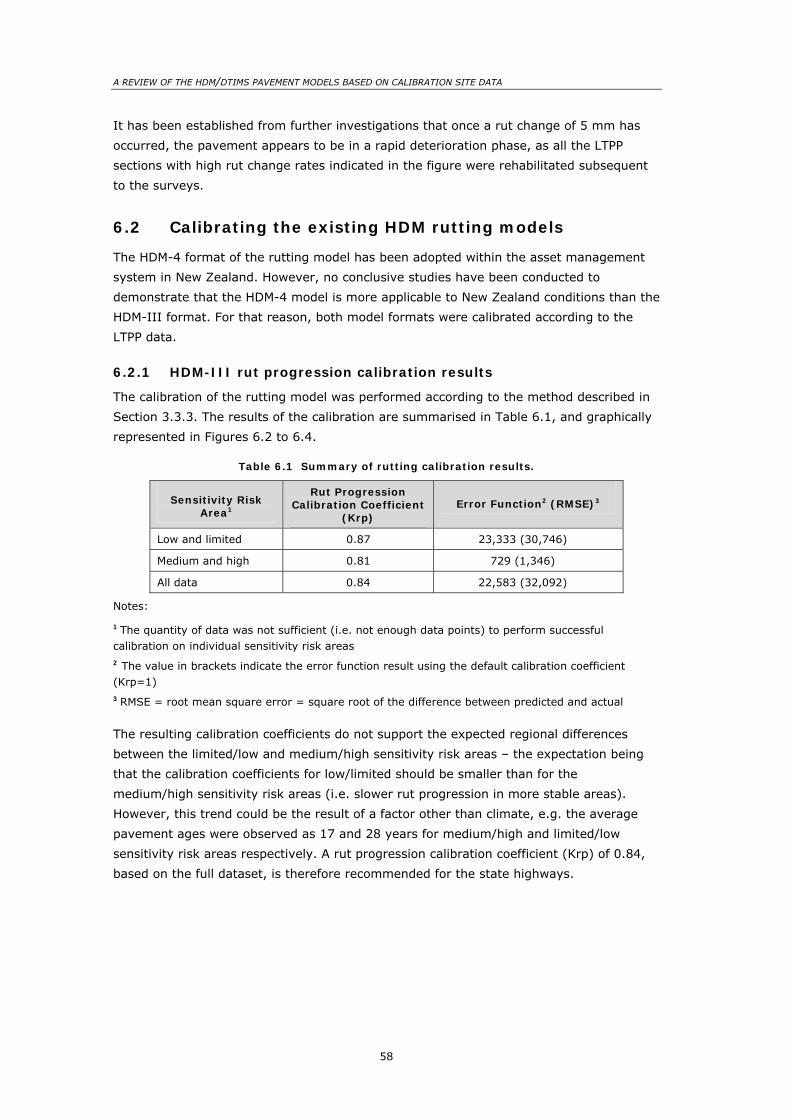
A REVIEW OF THE HDM/DTIMS PAVEMENT MODELS BASED ON CALIBRATION SITE DATA
58
It has been established from further investigations that once a rut change of 5 mm has
occurred, the pavement appears to be in a rapid deterioration phase, as all the LTPP
sections with high rut change rates indicated in the figure were rehabilitated subsequent
to the surveys.
6.2 Calibrating the existing HDM rutting models
The HDM-4 format of the rutting model has been adopted within the asset management
system in New Zealand. However, no conclusive studies have been conducted to
demonstrate that the HDM-4 model is more applicable to New Zealand conditions than the
HDM-III format. For that reason, both model formats were calibrated according to the
LTPP data.
6.2.1 HDM-III rut progression calibration results
The calibration of the rutting model was performed according to the method described in
Section 3.3.3. The results of the calibration are summarised in Table 6.1, and graphically
represented in Figures 6.2 to 6.4.
Table 6.1 Summary of rutting calibration results.
Sensitivity Risk Area1
Rut Progression Calibration Coefficient
(Krp) Error Function2 (RMSE)3
Low and limited 0.87 23,333 (30,746)
Medium and high 0.81 729 (1,346)
All data 0.84 22,583 (32,092)
Notes:
1 The quantity of data was not sufficient (i.e. not enough data points) to perform successful calibration on individual sensitivity risk areas 2 The value in brackets indicate the error function result using the default calibration coefficient (Krp=1) 3 RMSE = root mean square error = square root of the difference between predicted and actual
The resulting calibration coefficients do not support the expected regional differences
between the limited/low and medium/high sensitivity risk areas – the expectation being
that the calibration coefficients for low/limited should be smaller than for the
medium/high sensitivity risk areas (i.e. slower rut progression in more stable areas).
However, this trend could be the result of a factor other than climate, e.g. the average
pavement ages were observed as 17 and 28 years for medium/high and limited/low
sensitivity risk areas respectively. A rut progression calibration coefficient (Krp) of 0.84,
based on the full dataset, is therefore recommended for the state highways.

6. Rutting
59
Predicted vs. Observed Rut Depth (Calibrated for high-medium)
2 4 6 8 10 12 14 16 18 20 22 24
Observed Rut Depth
2
4
6
8
10
12
14
16
18
20
22
24
Pre
dict
ed R
ut D
epth
Minimised Error Function (RMSE) = 729Number of observations = 132
Figure 6.2 Comparing the observed and predicted rut depth for the calibrated model (high and medium sensitivity areas).
Obsreved vs. Predicted Rut Depth (Low-Limted sens)
0 2 4 6 8 10 12 14 16 18 20 22 24
Observed Rut Depth
0
2
4
6
8
10
12
14
16
18
20
22
24
Pre
dict
ed R
ut D
epth
Minimised error funtion (RMSE) = 23 333Number of Observations = 252
Figure 6.3 Comparing the observed and predicted rut depth for the calibrated model (limited and low sensitivity areas).
Figures 6.2 and 6.3 depict the comparison between predicted and observed rut depths.
The limited and low sensitivity risk areas have a better fit compared to the medium and
high sensitivityareas.
On both these graphs the correlation between the predicted and the actual data is within
the expected range (approximately ± 2 mm). However, if the predicted and actual

A REVIEW OF THE HDM/DTIMS PAVEMENT MODELS BASED ON CALIBRATION SITE DATA
60
incremental rutting change is compared, then the correlation seems to be much worse.
For example, Figure 6.4 illustrates similar data to Figure 6.3, but only shows the
incremental change in rutting from one year to another. Even though the calibration
yielded acceptable results, the recommendation is to review the rutting model format in
order to establish a better correlation between the model and actual pavement behaviour.
-4 -2 0 2 4 6 8
Observed Incrmental Rut Change (mm)
0
1
2
3
4
5
6
7
8
Pre
dict
ed In
crem
enta
l Rut
Cha
nge
(mm
)
Figure 6.4 Comparing the observed and predicted rut depth incremental change for the calibrated model (limited and low sensitivity areas).
6.2.2 HDM-4 Rut progression calibration results
Table 6.2 lists the resulting calibration coefficients for the rut progression model as
defined in HDM-4. It suggests that the default model closely resembles the actual
behaviour of pavements in New Zealand, since the required calibration coefficients are
close to the default value of 1. In addition, the error function is small in comparison with
the outcome from the HDM-III rut model. This can be largely explained by a more normal
distribution of observed and predicted points centred around the line of equality
(Figure 6.5).
Table 6.2 Summary of rutting calibration results HDM-4.
Sensitivity Risk Area1
Rut Progression Calibration Coefficient
(Krp) Error Function2 (RMSE)3-
Low and Limited 1.03 2,719 (2,729)
Medium and High 0.98 931 (933)
All Data 1.01 3,658 (3662)
Notes:
1 The quantity of data was not sufficient (i.e. not enough data points) to perform successful calibration on individual sensitivity risk areas 2 The value in brackets indicate the error function result using the default calibration coefficient (Krp=1) 3 RMSE = root mean square error = square root of the difference between predicted and actual

6. Rutting
61
0 2 4 6 8 10 12 14 16 18 20 22
Observed Rut Depth (m m)
0
2
4
6
8
10
12
14
16
18
20
22
Pred
icte
d R
ut D
epth
(mm
)
Minim ised Error Function (RMSE = 3657.7)Number of Observations = 813
Figure 6.5 Comparing the observed and predicted rut depth for the calibrated HDM-4 model (all data points).
Figure 6.6 depicts the predicted and observed incremental rut change. This figure
suggests that the predicted incremental change varies very little around the average
prediction of about 0.3 mm to 0.4 mm per year.
-4 -2 0 2 4 6 8 10 12
Obeserved Increm ental Rut Change (m m /year)
0
1
2
3
4
5
6
7
8
Pre
dict
ed In
crem
enta
l Rut
Cha
nge
(mm
/yea
r)
Figure 6.6 Comparing the observed and predicted rut depth incremental change for the calibrated HDM-4 model (all data).

A REVIEW OF THE HDM/DTIMS PAVEMENT MODELS BASED ON CALIBRATION SITE DATA
62
6.3 Refining the rut progression model
6.3.1 Description of the data
Four years of surveyed rutting data have been used for the analysis presented in this
section. Because of accuracy requirements, only LTPP data were used for the analysis
(see Section 2.3). Figure 6.7 illustrates the incremental rut change measured. Survey
numbers indicated in the figure represent the delta rut between two surveys (e.g. 2 is the
incremental rut difference between survey 1 and 2). The figure depicts a growing rut change for each survey. Note that all negative rut
changes, corresponding with rehabilitations, were excluded from the analysis. Note that,
although the rutting has increased for the last survey period, the outliers in the data have
decreased significantly. Although the equipment used has remained the same, some
improvements were made to make the equipment more stable during the surveys.
2 3 4
-20
24
68
10
Survey Period
Incr
emen
tal R
ut C
hang
e
Figure 6.7 Incremental rut change.
6.3.2 Variable analysis
The variables considered during the analysis in the following sections are shown in
Table 6.3.

6. Rutting
63
Table 6.3 Variables considered for predicting rut progression.
Variable Description Variable Type
AADT Annual average daily traffic Continuous
YE4 Annual number of equivalent standard axles (millions/lane)
Continuous
SNP Structural number of the pavement Continuous
MMP Mean monthly precipitation Continuous
wpiri Wheel path IRI (mm/km) Continuous
HTOT Total surface thickness (mm) of all the layers Continuous
Sens Climatic sensitivity area Factor
AGE3 Age of the pavement (years) Continuous
AGE 2 Age of the surface Continuous
OTCI Time to crack initiation Continuous
Stat.crx Cracked status Binary
D0-D9 FWD-deflections for given geophones (micro mm) Continuous
maxdef FWD-maximum deflection from all geophones (micro mm)
Continuous
SF1 & SF2 FWD- deflection shape Factor 1 and 2 Continuous
SCI FWD- surface curvature index Continuous
BCI FWD- base curvature index Continuous
BDI FWD- base damage index Continuous
In terms of the stratified data, not much difference was observed between the average
incremental rutting for different climatic regions and for the cracked status of the
pavement (see Figure 6.8).
H L
-20
24
68
10
Climatic Sensitivity Area
Incr
emen
tal R
ut C
hang
e
FALSE TRUE
-20
24
68
10
Cracked?
Incr
emen
tal R
ut C
hang
e
Figure 6.8 Incremental rut change for stratified data.
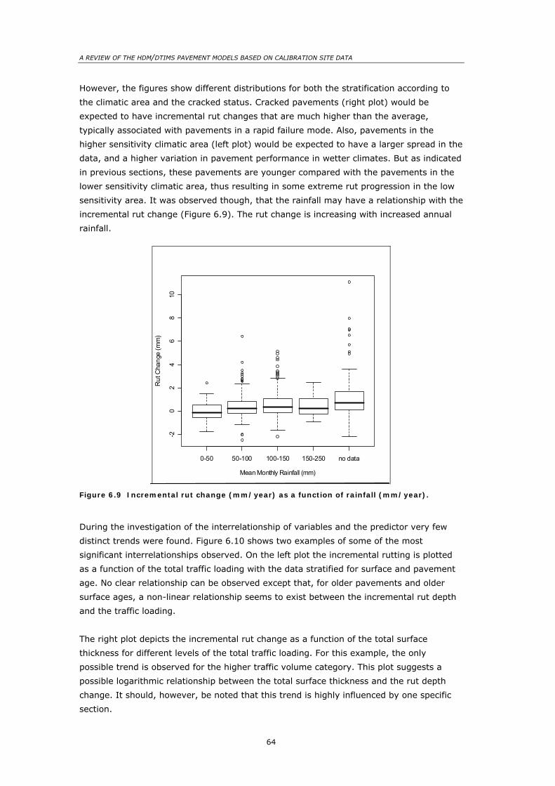
A REVIEW OF THE HDM/DTIMS PAVEMENT MODELS BASED ON CALIBRATION SITE DATA
64
However, the figures show different distributions for both the stratification according to
the climatic area and the cracked status. Cracked pavements (right plot) would be
expected to have incremental rut changes that are much higher than the average,
typically associated with pavements in a rapid failure mode. Also, pavements in the
higher sensitivity climatic area (left plot) would be expected to have a larger spread in the
data, and a higher variation in pavement performance in wetter climates. But as indicated
in previous sections, these pavements are younger compared with the pavements in the
lower sensitivity climatic area, thus resulting in some extreme rut progression in the low
sensitivity area. It was observed though, that the rainfall may have a relationship with the
incremental rut change (Figure 6.9). The rut change is increasing with increased annual
rainfall.
0-50 50-100 100-150 150-250 no data
-20
24
68
10
Mean Monthly Rainfall (mm)
Rut
Cha
nge
(mm
)
Figure 6.9 Incremental rut change (mm/year) as a function of rainfall (mm/year).
During the investigation of the interrelationship of variables and the predictor very few
distinct trends were found. Figure 6.10 shows two examples of some of the most
significant interrelationships observed. On the left plot the incremental rutting is plotted
as a function of the total traffic loading with the data stratified for surface and pavement
age. No clear relationship can be observed except that, for older pavements and older
surface ages, a non-linear relationship seems to exist between the incremental rut depth
and the traffic loading.
The right plot depicts the incremental rut change as a function of the total surface
thickness for different levels of the total traffic loading. For this example, the only
possible trend is observed for the higher traffic volume category. This plot suggests a
possible logarithmic relationship between the total surface thickness and the rut depth
change. It should, however, be noted that this trend is highly influenced by one specific
section.

6. Rutting
65
In summary, no conclusive trends were observed for the variable analysis.
-20
24
68
10
0.00 0.01 0.02 0.03 0.04
0.00 0.01 0.02 0.03 0.04
-20
24
68
10
Traffic Loading (YE4)
Incr
emen
tal R
ut C
hang
e (m
m/y
r)
2 4 6 8 10 12 14
Given : Surface Age
050
100
150
Giv
en :
Pav
emen
t Age
-20
24
68
100 20 40 60 80 100 120
0 20 40 60 80 100 120
-20
24
68
10
Total Surface Thickness
Incr
emen
tal R
ut C
hang
e (m
m/y
r)
0.00 0.05 0.10 0.15 0.20 0.25 0.30
Given : Total traffic Loading - YE4
Figure 6.10 Testing the interrelationships of variables affecting rut change.
6.3.3 Linear model (LM) regression analysis results
A stepwise regression was performed according to the same approach as explained in
Section 4.2.5. Table 6.4 lists each step of the regression process and its effect on the AIC
(Akaike’s Information Criterion). The AIC is like a fault term with the lower values
indicating better fit with the observed data. See also Appendix D (Figure D.1) for the
resulting model coefficients and model diagnostic plots. The resulting model has an
overall R2 of 0.4 and most variables included to the regression were found to be
significant.
The table also indicates that most variables included in the model are able to improve the
AIC, thus suggesting that the model is significantly contributing towards explaining the
independent variable (rut progression). This phenomenon is typical of a trend that has no
distinct variable/s explaining it. Also, it is observed that multiplication of variables
significantly drops the AIC. Each step, including a multiplication, reduces the AIC more
than any individual variable. This confirms the model approach as suggested in HDM-4
(see Section 3.3.3.1).

A REVIEW OF THE HDM/DTIMS PAVEMENT MODELS BASED ON CALIBRATION SITE DATA
66
Table 6.4 ANOVA (analysis of variance) results from linear model regression for rut
progression.
Step Step Factor Deviance Residuals Deviation AIC
1 intercept 1153.4 338.0
2 mmp 54.06 1099.3 305.2
3 ye4 39.02 1060.3 281.0
4 snp 20.60 1039.7 268.7
5 ye4:snp 110.06 929.6 189.5
6 age3 10.61 919.0 183.1
7 ye4:age3 29.57 889.4 161.4
8 sf2 6.71 882.7 157.9
9 ye4:sf2 89.06 793.7 82.7
10 age3:sf2 19.23 774.4 66.9
11 age2 9.47 765.0 60.0
12 ye4:age2 4.88 760.1 57.3
13 adt 5.81 754.3 53.7
14 sci 5.83 748.5 50.1
15 age3:sci 15.73 732.7 36.7
16 ye4:sci 4.47 728.3 34.2
17 sf2:sci 7.84 720.4 28.4
18 bci 16.93 703.5 13.1
19 age2:bci 14.12 689.4 0.4
20 ye4:bci 6.52 682.8 −4.5
21 sci:bci 7.87 675.0 −10.9
22 age2:sci 5.54 669.4 −14.9
23 ye4:sf2 1.11 670.5 −15.7
24 sf1 2.26 668.3 −16.1
25 age2:sf1 6.43 661.8 −21.2
26 (-)age2:sci 0.21 662.1 −22.9
Figure 6.11 illustrates the difference between the predicted and observed rut depth for
the resulting model. This figure looks similar to Figure 6.4 in the sense that it has a
cluster of data concentrated around the average of the predictor, and beyond that point,
very little predictive power. This means that if we want to predict the incremental rut
change, we may just assume it to be equal to the average, say 0.3 mm per year.
Although an average rut progression rate does not incorporate changing variables, this
model simplification may well be adopted within the New Zealand modelling approach. It
is important though, to confirm this progression rate with more data.

6. Rutting
67
-2 0 2 4 6
-20
24
68
10
Predicted Incremental Rut Change
Obs
erve
d R
ut C
hang
e
Figure 6.11 Comparing the predicted and observed incremental rut change.
6.3.4 Future development requirements for rut progression model
• Investigate rut progression model forms on the CAPTIF data. Two major trends
must be investigated:
- Determine the factors contributing towards stable rut progression observed
during most of the pavement life. In particular see if the CAPTIF data confirms
the constant 0.3-mm rut progression of pavements. - Determine the factors contributing towards a pavement that starts accelerated
deterioration including a rapid rut progression. • Further tracking of rutting on individual sections over time. Since the LTPP data are
becoming available for longer time periods, this analysis would become more
useful. Also, by combining trends from the LTPP data and the CAPTIF data, it may
be possible to develop model formats from basic principles.
6.4 Rut depth standard deviation
The standard deviation of rut depth (rds) is used in the roughness model. At present, it is
calculated from the mean total rut depth (rdm) and has two forms, the HDM model
(NDLI 1995):
( )max 0.3, 0.9 0.04rds rdm rdm= −⎡ ⎤⎣ ⎦ (Equation 6.1)
and the New Zealand model (HTC 1999).
0.21 0.69rds rdm= + (Equation 6.2)
Using the test data, each of these models is reviewed, and a new one is proposed.

A REVIEW OF THE HDM/DTIMS PAVEMENT MODELS BASED ON CALIBRATION SITE DATA
68
Figure 6.12 shows the relationship between rdm and rds. It is clear that a log transform
of both variables (the right-hand plot) displays a more normally distributed linear trend.
This is also intuitively obvious, as rds is strictly positive and skewed towards the right
(likewise for rdm). It should be noted here that none of the existing models utilise this
basic property of variance.
5 10 15 20 25
05
1015
2025
rdm
rds
1.0 1.5 2.0 2.5 3.0-1
01
23
log(rdm)
log(
rds)
Figure 6.12 Plots showing the relationship between rdm and rds. (The plot on the right-hand side displays a log transform of both variables.)
The basic model developed in this report uses the log transforms of rds and rdm (referred
to as Model 1). Using standard linear regression the fitted model was found to be:
( ) ( )( )
2log 0.8804log 0.9369 0.49
exp 0.8804log 0.9369
rds rdm R
rds rdm
= − =
= −⎡ ⎤⎣ ⎦ (Equations 6.3 and 6.4)
with model diagnostics given in Appendix D.
Figure 6.13 shows the model fit to the observed data (left-hand plot) and a comparison of
all three models (right-hand plot). It is clear that the HDM.RDS model is not appropriate
for New Zealand use. Comparing the other two models, the NZ.RDS shows an increasing
linear trend, while Model 1 shows an increasing concave function. Further, Model 1 decays
to zero (i.e. the y intercept) while the NZ.RDS model shows a positive y intercept, which
is clearly impossible. Another feature of the new model is that the variance structure is
multiplicative as opposed to additive. Therefore, as RDM increases, so does the variance
around RDS. This suggests that any deterministic prediction of the RDS based on large
values of RDM is somewhat questionable, and should possibly be based on a more
probabilistic approach.

6. Rutting
69
0 5 10 15 20 25
05
1015
rdm
rds
DataFitted Model97.5% Prediction Level
0 5 10 15 20 25
05
1015
rdm
rds
DataFitted ModelNZ.rdsHDM.rds
Figure 6.13 Plots of model fit and comparison between models.

A REVIEW OF THE HDM/DTIMS PAVEMENT MODELS BASED ON CALIBRATION SITE DATA
70
7. Roughness
7.1 LTPP roughness data
The HMD-4 roughness model format was developed with the underlying philosophy that
the roughness will always increase incrementally, regardless of how lightly the pavement
is loaded or how minor the environmental effects may be. This trend could not be
supported by the actual data, and as a result the calibration of the roughness model was
not possible. Figure 7.1 illustrates the distribution of incremental roughness change
between the three surveys. This figure suggests that hardly any change in roughness
occurs from one year to another for most of the sections.
Incremental Roughness Change (IRI)
Num
ber o
f 100
m
Subs
ectio
ns
Survey Period: Oct 02 - Feb 03
-1.2-1.0
-0.8-0.6
-0.4-0.2
0.00.2
0.40.6
0.81.0
1.21.4
0
20
40
60
80
100
120
140
160
180
Survey Period: Oct 03 - Feb 04
-1.2-1.0
-0.8-0.6
-0.4-0.2
0.00.2
0.40.6
0.81.0
1.21.4
Figure 7.1 Distribution of incremental roughness.
It is further noted that the distribution of the roughness change between the 2002 and
2003 survey rounds is wider than between the 2003 and 2004 survey rounds. According
to the site notes, many of the negative changes (i.e. roughness improvements) for the
2002 to 2003 survey periods could be explained by texture loss on newly resurfaced
roads, and flushing on older pavements. These effects were less pronounced in the 2003
to 2004 survey rounds because of less resurfacing in that period.
Given that the accuracy of the roughness measurements is specified at ± 0.2 IRI
(Transit 2001, Henning et al. 2004a), any measurements within this tolerance do not
necessarily indicate a trend towards improvement or deterioration. Referring to
Figure 3.3, this would suggest that, for most of the measurements, the roughness can be
assumed not to have changed at all. Where section data indicated a definite change in
roughness, this was usually explained by the survey field notes. For example, where the

7. Roughness
71
roughness improved, obvious signs of flushing or texture loss were present. Sections that
showed clear indications of roughness deterioration were in a rapid deterioration phase,
and most of these sections were rehabilitated shortly following the surveys. Given the above, it was not surprising that any attempt to calibrate the existing HDM
model did not yield satisfactory results, from which it was concluded that the roughness
model format probably needed adjustment as discussed in Section 7.2.
7.2 A review of the roughness model
7.2.1 Environmental component
It is recognised that roughness sometimes increases because of environmental effects
only. This is very applicable to New Zealand conditions, given the geological makeup.
Even if no traffic travels on certain roads, the roughness will increase. A good example of
in-situ material where this phenomenon is common is the peat areas in the Waikato.
However, in most cases the total roughness progression is very low, and one would
therefore expect the environmental component of the deterioration to be even smaller.
Little work has been undertaken in New Zealand in order to understand the environmental
impact on roughness. This research would take a very long time, and understanding some
of the more significant variables of the model first would be useful before such a study is
undertaken.
7.2.2 Structural component
The structural component of the roughness model is of main interest for this study. This
model is of the following format (NDLI 1995):
YE4SNPK)AGE3)(1exp(mK*aΔRI 5gm0S
−+= (Equation 7.1)
where:
∆RIs structural component of roughness change
a0 model coefficient
m environmental coefficient
Kgm environmental calibration coefficient
AGE3 pavement age
SNPK structural number including crack influence
YE4 annual number of equivalent standard axles (millions/lane)
The influence of the strength component is illustrated in Figure 7.2. Also indicated in the
figure is the relative influence of the strength component in the rutting model.

A REVIEW OF THE HDM/DTIMS PAVEMENT MODELS BASED ON CALIBRATION SITE DATA
72
0
0.05
0.1
0.15
0.2
0.25
0.3
0.35
0.4
0.45
0.05 0.1 0.2 0.4 0.8 1.6
Annual Axle Loading (million equevalent axles /year)
Incr
emen
tal R
ut C
hang
e (m
m/y
ear)
-0.005
0.005
0.015
0.025
0.035
0.045
0.055
0.065
0.075
Incr
emen
tal R
ough
ness
Cha
nge
(IRI/Y
ear)
Incremental Rut Change Incremental Roughness Change
Figure 7.2 Comparing the influence of the strength component on roughness and rutting change (Note, in both cases a pavement age of 10 years was assumed).
Observations from this figure are:
• The strength component in the roughness model is significantly more sensitive for
increasing traffic loading compared to the strength component in the rutting model.
Although the scale is different for the two parameters, the figure shows an
exponential growth of the roughness model because of the strength component;
• The incremental change for the roughness model is very low if compared with the
expected accuracy achievable with roughness survey equipment. Calibrating
according to such low incremental changes has proven to be problematic.
Therefore, we are trying to predict annual changes which we cannot observe, even
by using the most accurate instruments in the industry.
7.2.3 Incremental change caused by rutting
The interaction between rutting and roughness is well observed for network data in New
Zealand. However, evidence of initial reduction in rutting variation exists during the early
years of pavement life (see Section 6.3). The rutting, in combination with some macro
texture effects, is therefore contributing towards an initial reduction of roughness, which
is not recognised in the roughness model.
7.3 Proposed changes to the roughness model
Most network analysis performed in New Zealand has suggested difficulties in calibrating
the roughness model, or in obtaining meaningful roughness prediction from the modelling
system (MWH 2004). In most cases, very low calibration coefficients are used, and
regardless of the maintenance quantities scheduled, the roughness deteriorates for the
network.
Observing the LTPP data also suggests that the roughness progression is somewhat
different from the HDM model. Figure 7.3 illustrates this difference diagrammatically.

7. Roughness
73
Traffic Loading or Time
Rou
ghne
ss P
rogr
essi
onGradual Deterioration
Phase
Initial DensificationPhase
Rapid Deteriorationphase
Rapid FailureInitialisation
Classic roughness progression of unbound granularpavements e.g. HDM
Observe Roughness Distribution
Note: The figure is based on very limited data and is only applicable to chipseal pavements
Figure 7.3 Schematic comparison between the HDM roughness model and observed behaviour in New Zealand.
The HDM model would, in most circumstances, predict a continuous roughness
progression, even if very low calibration coefficients are selected. The actual roughness
data from the LTPP database suggests the following differences:
• Evidence exists of an initial reduction in roughness following construction and
resurfacing. The significant reduction of roughness following resurfacing is believed
to be caused by the re-orientation of chip, and is more prominently observed for
Walking Profilometer measurements used on the LTPP sites (see Figure 7.4). This
trend is less evident for HSD type measurements undertaken on the same sections.
However, a reduction in roughness still occurs initially following construction. This
trend correlates with the initial reduction in rut depth standard deviation.
• Following the initial 'settling-in' phase, the roughness remains unchanged for a very
long time. For example, hardly any roughness change can be observed on low
volume roads for a significant period of time. This will only change when the
pavement reaches the end of its capacity life, the traffic changes significantly, or
when water enters the pavement (Land Transport New Zealand 2005). After this
the pavement goes into a rapid failure mode, which is characterised by an
exponential roughness progression rate.
The model form described above and illustrated in the figure is not uncommon in the
engineering industry. It is often referred to as the 'bath tub' model format, which signifies
the performance of most mechanical components such as motor engines etc. Should this
model format be appropriate for New Zealand, the focus of the model will change from
'how much does the roughness change in a year?' to 'when does the rapid deterioration
start?' It is recognised that the classic HDM roughness model may still be valid for some
pavement types and pavements constructed for higher volume roads.

A REVIEW OF THE HDM/DTIMS PAVEMENT MODELS BASED ON CALIBRATION SITE DATA
74
0
5
10
15
20
25
30
35
40
45
50
<-1.2 -1.0 to-1.2
-0.8 to-1.0
-0.6 to-0.8
-0.4 to-0.6
-0.2 to-0.4
0 to -0.2
0 to+0.2
0.2 to+0.4
0.4 to+0.6
0.6 to+0.8
0.8 to+1.0
1.0 to+1.2
>1.2
Change in IRI Distribution
Perc
enta
ge o
f Sec
tions
Calibration Benchmark Figure 7.4 Comparing the incremental roughness change between LTPP data (calibration) and HSD data (benchmark) (Transit 2005).
During the past three years only two LTPP sections have progressed to this rapid
deterioration stage. It will take at least five to ten years before the LTPP experiment will
have sufficient data available to develop the proposed model format. However, by
combining the LTPP data with the Transit CAPTIF (Canterbury Accelerated Pavement
Testing Indoor Facility) data, it would be possible to investigate the merits of such a
model further. A research study to do that has been approved for the 2005/06 financial
year. For that reason, this report will not discuss the roughness model any further.

8. Recommendations
75
8. Recommendations
8.1 The future of the New Zealand LTPP sections
This report has demonstrated that the level of data collection accuracy is appropriate for
calibration and pavement model development. Some intuitive trends with some models
(such as roughness) have been confirmed for the first time since the appropriate level of
data accuracy existed. However, this study has also highlighted the need for further
model development based on an individual section data. It has been suggested that some
of the models such as roughness and rutting could be developed utilising some CAPTIF
data, but ultimately could only be confirmed with the LTPP data.
Furthermore, the report has highlighted the significance of the rapid failure stages of
pavement deterioration modelling. To understand the behaviour during rapid deterioration
better, more data during this stage are needed.
The recommendation is therefore that the LTPP surveys continue on both the Transit and
local authority networks. It is difficult to put a time period on the required survey
duration, but the period estimated is at least another five years.
In terms of the current data collection precision and accuracy requirements, the
recommendation is that the current standard be maintained.
8.2 Investigate the rapid failure stage for roughness and rutting progression
As a next stage to this research, a proposal was accepted for the 2005/06 Land Transport
New Zealand Research Programme. This study is aimed at linking both the LTPP and the
CAPTIF programmes. The objectives of this research are explained in the extract from the
research proposal:
Linking the outputs from CAPTIF with the LTPP study is the next logical step
towards building on the understanding of pavement performance/
deterioration under New Zealand conditions. Comparing field performance
(LTPP) with the accelerated load performance (CAPTIF) will significantly
increase the confidence in outputs from both these programmes. The specific
objectives of the study include:
1. Calibration coefficients and new model formats have been developed
based on the Transit LTPP data (Transfund Research Programme
04/05). The first objective would be to confirm and improve the model
format and results based on existing CAPTIF data;
2. To develop relative performance factors for different treatments and
material types, similar to the work completed in Australia (Martin
et al 2004). It should be appreciated that the data from both

A REVIEW OF THE HDM/DTIMS PAVEMENT MODELS BASED ON CALIBRATION SITE DATA
76
programmes will greatly extend the range of applicability of both
programmes;
3. To gain a better understanding of the environmental impact on
pavements. The LTPP sections are subjected to normal climatic
influences whereas the CAPTIF testing was conducted under controlled
conditions. It is therefore possible to investigate the specific
environmental impacts on pavement performance, something which is
relatively complex to do based on LTPP work alone; and
4. Confirm CAPTIF life cycle and mass limit study results with the LTPP
performance data.5
An obvious emphasis of this study would be to increase the understanding of the
deterioration of the pavement during the rapid failure stages.
8.3 Introducing uncertainty and statistical distribution in some models
According to some network experience combined with engineering observations, some of
the pavement behaviour cannot be explained according to deterministic model formats.
For example, this report has suggested a generalised linear model format for predicting
cracking. Likewise, defects such as potholing and failures (shoving) would be easy to fit
according to some statistical distribution such as a Proportional Intensity Model.
This change in modelling approach would not be transferable, similar to the HDM
approach. However, it would produce modelling outcomes that more closely resemble
actual behaviour in New Zealand.
It is recommended that this development is undertaken as part of the dTIMS CT
development consortium tasks, since it will optimise the input from all practitioners in
New Zealand.
5 Research Proposal: Benchmarking pavement performance between Transit’s LTPP & CAPTIF
programmes 05/06 Research Round. MWH New Zealand Ltd.

9. References
77
9. References
Bennett, C.R., Paterson, W.D.O. 2000. A guide to the calibration and adaptation. HDM - 4.
Volume 5. The Highway Development and Management Series. PIARC.
Cenek, P.D. 2001. Summary report- Regionalisation of roading authorities for pavement
deterioration modelling. Memorandum to Ken Hudson. Opus Central Laboratories:
Lower Hutt, NZ.
Chambers, J.M., Hastie, T.J. 1992. Statistical Model in S. Chapman and Hall: London, UK.
Hallet, J.E., Tapper, M.S. 2000. Pavement modelling - Data input effects. Paper presented
at NZHIT Conference. Beca Carter Hollings & Ferner Ltd: Rotorua, New Zealand.
Henning, T.F.P., Costello, S.B., Dunn, R.C.M., Parkman, C.C., Hart, G. 2004a. The
establishment of a long-term pavement performance study on the New Zealand State
Highway Network. Road & Transport Research 13(2): 17-32.
Henning, T.F.P., Dunn, R.C.M., Costello, S.B., Hart, G., Parkman, C.C., Burgess G. 2004b.
Long-term pavement performance (LTPP) studies in New Zealand – Lessons, the
challenges and the way ahead. Proceedings of the 6th International Conference for
Managing Pavements: Brisbane, Australia.
Henning, T.F.P., Riley, M. 2000. Calibration guidelines for pavement deterioration models
and work effects models in dTIMS. HTC Infrastructure Management. Auckland,
New Zealand.
Henning, T.F.P., Tapper, M. 2004. Calibration of pavement deterioration models based on
the 2003 calibration data. Special study completed by MWH New Zealand Ltd and Beca
Carter Hollings & Ferner Ltd. The Asset Management Team, Transit New Zealand:
Wellington, New Zealand.
Henning, T.F.P., Visser, A.T., Sadzik, E.S. 1998. An attempt to calibrate HDM-III
prediction models on the basis of PMS data. CAPSA 1999. SABITA, South Africa.
HTC Infrastructure Management. 1999. Technical reference manual Volume I. HTC
Infrastructure Management: Auckland, New Zealand.
Koniditsiotis, C., Kumar, A. 2004. Prediction of road pavement structural capacity from
transverse profile shape. Proceedings of the 6th International Conference for Managing
Pavements: Brisbane, Australia.
Land Transport New Zealand. 2005. dTIMS CT conceptual development for low volume
roads. Technical report completed by the dTIMS CT Development Consortium. MWH
New Zealand Ltd: Auckland, New Zealand.

A REVIEW OF THE HDM/DTIMS PAVEMENT MODELS BASED ON CALIBRATION SITE DATA
78
Martin, T.C., Toole, T., Oliver, J.W.H. 2004. The development of HDM-4 technology road
deterioration models for Australia's sealed granular pavements. 6th International
Conference for Managing Pavements: Brisbane, Australia.
MWH New Zealand Ltd. 2004. Appendix 18 – TNZ Region 9 (Wellington) dTIMS analysis.
Transit New Zealand: Wellington, New Zealand.
NDLI. 1995. Modelling road deterioration and maintenance effects in HDM-4. Final Report
ADB BETA 5549. Vancouver, BC, Canada.
Oliver, J.W.H. 2004. Prediction of the life of sprayed seals and the effect of climate,
durability and seal size. 6th International Conference for Managing Pavements:
Brisbane, Australia.
Paterson, W.D.O., Attoh-Okine, B. 1992. Simplified models of paved road deterioration
based on HDM-III. Transportation Research Board, 71st Annual Meeting: Washington,
DC, USA.
Rohde, G.T., Jooste, F., Sadzik, E.S., Henning, T.F.P. 1998. The calibration and use of
HDM-4 performance models in a pavement management system. 4th International
Conference on Managing Pavements. ICC: Durban, South Africa.
Rohde, G.T., Wolmerans, I., Sadzik, E.S. 2002. The calibration and validation of HDM
performance models in the Gauteng PMS. 21st Annual South African Transport
Conference. CSIR: South Africa.
Transit New Zealand. 2001. Transit New Zealand calibration sections survey contract
number TNZ SM3-688/P6/10. Transit New Zealand: Napier, New Zealand.
Transit New Zealand. 2003. Safety related surface issues final report. Special study
completed by MWH New Zealand Ltd and Opus International Consultants. The Asset
Management Team, Transit New Zealand: Wellington, New Zealand.
Transit New Zealand 2004. Calibration of pavement deterioration models based on the
2003 calibration data. Special study completed by MWH New Zealand Ltd and Beca
Carter Hollings & Ferner Ltd. The Asset Management Team, Transit New Zealand:
Wellington, New Zealand.
Transit New Zealand. 2005. Benchmarking Transit high speed surveys with calibration
surveys. Special study completed by MWH New Zealand Ltd. The Asset Management
Team, Transit New Zealand: Wellington, New Zealand.
Watanatada, T., Harral, C.G., Paterson, W.D.O., Dhareshwar, A.M., Bhandari, A.,
Tsunokawa, K. 1987. The highway design and maintenance standards model. World
Bank. The John Hopkins University Press: Baltimore, Maryland, US.

Appendix A
79
Appendix A Paper on the establishment of the LTPP programmes
Long-term Pavement Performance (LTPP) Studies in New Zealand – Lessons, the
Challenges and the Way Ahead
Henning T.F.P.1, Dunn R.C.M.2, Costello S.B. 2, Hart G.3, Parkman C.C.3 and Burgess G.4
1. MWH New Zealand Ltd., Auckland
2. The University of Auckland
3. Transit New Zealand
4. Transfund New Zealand, Christchurch
SYNOPSIS
New Zealand embarked on a Long-Term Pavement Performance (LTPP) programme with the establishment of 63 LTPP sites on the State Highway network during 2000. In 2003, this programme was expanded to include more than 21 local road controlling agencies by instituting a further 82 LTPP sites. By including rural sites and low volume rural roads in the study, the LTPP programme now covers a wide spectrum of pavement construction, traffic composition and climatic zones experienced in NZ. Before commencement in New Zealand, earlier LTPP studies undertaken overseas were reviewed, namely: World Bank Highway Design and Maintenance Standards (HDM-III) study in Brazil, the Strategic Highway Research Programme (SHRP) in the USA and International Study of Highway Development and Management (ISOHDM) calibration studies performed in both Australia and South Africa. This paper describes the many cases where new principles and ideas have been applied to address the specific challenges presented by the New Zealand roading environment. As an example, a performance based survey contract was developed for this project in order to achieve the accuracy requirements for the data collection. The value of reviewing international ‘best’ practice was most useful in developing the specific New Zealand LTPP study objectives, which were: 1. establish a representative sample of LTPP sections across New Zealand
considering the combined effects of climate and sub-soil moisture sensitivity; 2. enhance the existing data collection being undertaken on a network level; 3. collect data to a precision level suitable to perform incremental model calibration
and to adjust model formats if required.

A REVIEW OF THE HDM/DTIMS PAVEMENT MODELS BASED ON CALIBRATION SITE DATA
80
For the state highway study, a third round of surveys has been completed. Hence, it is now possible to assess the philosophy adopted for this New Zealand programme. This paper reviews the data collection methodology, relative to the original study objectives, assumptions and specifications. The statistical characteristics recorded for the design matrix factors for the state highway LTPP sections has indicated that the full range of expected values on the New Zealand network are being monitored. The statistics also show that there is a reasonably even distribution for most variables, thus not creating a bias towards the mean value. Furthermore, it is concluded that an appropriate level of data collection accuracy has been adopted for the New Zealand programme. At this early stage, the LTPP New Zealand programme has been successful in achieving the goals and objectives. On the other hand, a review of the data has highlighted areas where further research is required and proceeding – for example further work is required to confirm that all the main drivers that contribute to deterioration in the New Zealand environment are currently being recorded as part of the LTPP programme. The next major stage of the programme is to investigate the model format and determine the calibration requirements.

Appendix A
81
INTRODUCTION
Background to Pavement Deterioration Modelling in New Zealand During 1998, New Zealand significantly enhanced its asset management approach through the incorporation of predictive capabilities to forecast long-term pavement maintenance needs. A system consisting of an optimisation analysis process (dTIMS) was combined with the World Bank Highway Development and Management (ISOHDM) pavement deterioration models. The system has been adopted by Transit New Zealand and most of the 74 territorial road-controlling authorities throughout the country. Since initiation, it was realised that in order to achieve better correlation between the predictive models and actual pavement deterioration, it would be necessary to enhance current desk-top calibration of the models with actual long-term pavement performance studies (LTPP). In this regard, two LTPP studies are underway in New Zealand:
• Transit New Zealand established 63 sections on the state highways across the North and South Islands; and,
• Approximately 21 road controlling authorities have established a total of 82 sections in both urban and rural areas.
The Transit sections were surveyed for the first time in 2000. The survey of road controlling authority sections commenced in 2003. Transfund New Zealand, the funding agency for roading in New Zealand, is co-ordinating and managing the LTPP study for road controlling authorities. This paper documents the process of the experimental layout and planning of the LTPP studies which has been largely based on similar international studies.
Objectives of this Paper The main objectives of this paper are to outline and discuss the resulting experimental layout and data collection regime adopted. Secondly, to discuss the results from the data collected to date. This paper also gives an outline of the comprehensive literature review which was undertaken prior to the study. LTPP studies are a long-term investment therefore it is important to determine the appropriateness and relevance of the data at an early stage of the research project. Such concerns are discussed in this paper in an attempt to answer the following questions:
• Is the sample size sufficient? • Are all factors (independent variables) sufficiently covered with the
experimental layout (design matrix)? • Are the expected range for each factor measured? and, • Is the data collection methodology appropriate and is the precision of
measurements sufficiently accurate?

A REVIEW OF THE HDM/DTIMS PAVEMENT MODELS BASED ON CALIBRATION SITE DATA
82
SUMMARY OF INTERNATIONAL CALIBRATION STUDIES
Scope of Literature Review A literature review was undertaken on those LTPP studies which closely resembled the intended work in New Zealand. From the outset, the intention was to use the original HDM pavement models (Paterson, 1987) as a basis for the LTPP programme. This prompted the need to review the original HDM studies (GEIPOT, 1981) along with known calibration studies performed elsewhere to calibrate World Bank models, for example in South Africa and Australia (Rohde, et. al, 1998 and Tepper and Martin, 1999). In addition some non-HDM studies were reviewed, particularly in relation to the experimental design matrix and data collection regime for example USA and Australia (FHWA, 2000 and Martin, 1994).
Original Studies for HDM-III (Brazil) The World Bank HDM-III model is comprised of three different levels: a life-cycle maintenance analysis philosophy, pavement deterioration / work effects / road user cost models and lastly the analysis software. The Brazil study (GEIPOT, et. al, 1981) mainly focused on the development of the pavement and road user cost models. The primary interest in this Brazil study was the design matrix used for the site establishment, especially the road characterisation in the matrix. The technical team conducting this study was faced with similar objectives and constraints that most countries face during the planning stage of the experiment such as:
• The data had to be sufficient for statistical analyses but the study scope was limited by the total number of sections and the measurements to be taken; and,
• It was difficult to populate all the cells of a design matrix, such as, strong pavements on low volume roads.
The resulting design matrix for the Brazil study is depicted in Figure 1.

Appendix A
83
Figure 1: Design Matrix for the Paved Road HDM-III Study in Brazil (GEIPOT, et. al, 1981)
The numbers in the cells of the design matrix represent the section identification numbers and the study was conducted on a total of 65 test sections. Some pertinent observations obtained from the study included:
• The number of sections identified for the study 65, was the absolute minimum in order to perform reliable statistical analyses;
• The selected sections included in-service pavements and some specifically constructed pavements - the latter were constructed under controlled conditions;
• The design matrix included a factor for the maintenance regime - some of the pavements were subjected to normal maintenance while others only underwent emergency routine maintenance.
One aspect, which has been adopted in recent calibration studies including the New Zealand study, is the crack rating method. According to the HDM-III definition, cracks are measured linearly or according to the area, depending on crack type, and expressed as an area of the section affected by the cracking. The area effected by a linear crack is calculated by multiplying the length with a standard width of 0.5m.
Strategic Highway Research Programme (SHRP) LTPP study - USA The SHRP study (FHWA, 2000) is undoubtedly the most elaborate study of its kind ever conducted. Started in 1989, this LTPP programme is planned to observe pavements for a period of 20 years across the USA and Canada. As the SHRP study had a much wider scope compared to the intended studies in New Zealand, only relevant aspects of it were reviewed. Relevant to New Zealand was the long-term monitoring of in-service pavements. The objective for this study component of the SHRP program was to investigate the effect of loading, environment, material properties, construction quality and maintenance levels on the performance of pavements. Two aspects considered from the SHRP program, included the approach followed for the experimental design and the planning and documentation of data collection.

A REVIEW OF THE HDM/DTIMS PAVEMENT MODELS BASED ON CALIBRATION SITE DATA
84
Of specific interest was the review undertaken on the actual sections established versus the original design matrix. This approach was extended by Benson (1991) who has developed a technique to evaluate the success of the LTPP site establishment relative to the original design matrix and study objectives. For this review an effectiveness ratio was developed to test the variances of the expected versus the achieved variances of the sampling pattern. The effectiveness ratio is defined as:
Achieved VarianceMedian VarianceDesired100essEffectiven ×=
This effectiveness ratio has also been used in the identification of the priority cells (i.e. those cells which would be harder to populate) in the design matrix during the site establishment. Some of the Benson’s (1991) conclusions were:
• For cases where the factorial design was not balanced, regional model development must be considered due to the concern over the inference space;
• In cases where pavements with similar failure mechanisms exist, data for these sections could be combined in order to achieve better balances of factors in the design matrix;
• Regional data collection operations had to be reviewed in order to identify and illuminate sources of bias;
• Distributions have to be investigated to check for non-normality, bi-modalism and extreme cases.
Another important aspect of the SHRP-LTPP study (SHRP-LTPP, 1990 and 1999) was the detail to which data collection regimes and methods were specified. Appendix A summarises the pavement monitoring conducted for the study.
LTPP Studies in Australia Two LTPP studies conducted in Australia were reviewed:
• A study into the development of new pavement deterioration models (Martin, 1994) - this Australian Road Research Board (ARRB) study commenced during 1990 and one of the main focuses was to assist in the calculation of road agency expenditure (road track cost);
• A second study (Tepper and Martin, 1999) was the calibration of HDM–4 models - this study, also done by ARRB, included eight LTPP sections in Victoria, Queensland, New South Wales and Tasmania.
The first study was aimed at a strategic level and for this reason, network level type data collection was used (namely, high speed data) as opposed to a more detailed level as proposed for HDM calibration studies. This approach resulted in the affordability of a higher number of sections, 150 sections were surveyed. The second study was specifically designed to calibrate HDM-4 models. The study layout was also planned to focus on the work effects models. The work effects models predict the influence of different maintenance options on the immediate and long-term performance of the pavements. For this reason, the experiment consisted

Appendix A
85
of constructing sections of roads with different maintenance treatments - an example of the sections layout is given in Figure 2.
Figure 2: Example of Maintenance Treatments Applied on Australia’s LTPP Study Sections
(Tepper and Martin, 1999)
A falling weight deflectometer (FWD) was used for all strength measurements and the ARRB Multi-laser profilometer was used for measuring the longitudinal and transversal profiles. All the sections were tested prior to and on completion of the maintenance treatments. Subsequent measurements were also undertaken on an annual basis. Appendix B illustrates the section characteristics used in this ARRB HDM-4 study.
South Africa (Gautrans) HDM-III and HDM-4 Calibration Studies The Gauteng Provincial Government road department (Gautrans) initiated a LTPP study in 1993, which consisted of 36 sections (Rohde et al, 1998). A review of this study has been particularly useful for the New Zealand projects since it had similar objectives and it had been conducted over the last 10 years. Particular aspects of technical interest were:
• The design matrix that included factors such as traffic, base types, environments and pavement condition;
• Each site was 500m long and divided into 50m subsections; • The data collection regime on the sections consisted of test pit and FWD
measurements to quantify the pavement characteristics and a combination of manual rating, high speed data (HSD) roughness and manual rutting measurements to determine the condition data.
Appendix C illustrates the range of the parameters from the Gautrans LTPP sections. Ten years later, Rohde et al (2002) reviewed the calibration results and concluded the following:
• The original HDM-4 cracking model was satisfactory in its current form; • The rutting model format required improvement; • The roughness model performed satisfactorily • Overall, the pavement condition distribution predicted, correlated well with
the network trends and, therefore, was satisfactory for the PMS application

A REVIEW OF THE HDM/DTIMS PAVEMENT MODELS BASED ON CALIBRATION SITE DATA
86
In summary the results from the study suggested that the level of data accuracy was appropriate for the HDM model calibration coefficient adjustment. However, if a model format needed to be reviewed, then data collection at a higher level of accuracy would be required.
Summary of the LTPP Studies Review Below is a summary of the main aspects gained from the review of the international LTPP studies outlined in the previous sections.
Table 1: Relevant Issues from International LTPP Studies
Study Relevant Items New Zealand Context/Recommendation
The design matrix is simple and incorporates only major factors effecting pavement deterioration.
A similar approach applicable to New Zealand.
Specific pavements were built to monitor certain material types.
The New Zealand programme is to monitor in-service pavement deterioration
On sterilised sections only limited maintenance to ensure safety.
A similar approach applicable to New Zealand.
A well defined measure of visual crack detection was used
A similar approach applicable to New Zealand.
HDM-III – Brazil
Traffic monitoring was done at a high level A similar approach applicable to New Zealand.
The scope of the study was vast. The New Zealand programme is on a much smaller scale.
Multiple objectives were addressed with the study. Main objective is to investigate pavement performance.
Experimental design only considers major pavement deterioration factors.
A similar approach applicable to New Zealand.
An un-weighted stratified sampling method was used rather than a random method. The aim is to incorporate extreme points.
A similar approach applicable to New Zealand. SHRP-USA
An effectiveness ratio was developed to test the applicability of chosen sites, relative to the original design matrix.
A similar approach applicable to New Zealand.
Different maintenance treatments were tested within one section to determine work study effects.
The New Zealand programme is to monitor in-service pavement deterioration
Experimental layout effectively isolates certain factors on the design matrix e.g. everything else is the same while maintenance treatment is varied.
The New Zealand programme is to monitor in-service pavement deterioration. HDM-4 Australia
Mix of different LTPP site types were used –e.g. specially built and in-service pavements.
Good benchmarking for in-service and specific type pavements.
Experimental design only considers major pavement deterioration factors.
A similar approach applicable to New Zealand.
The site layout included 500m long sections divided into 50m sub-sections
A similar approach to be adopted in New Zealand. However a shorter total length will be used.
Visual Rating to include all HDM distresses. A similar approach applicable to New Zealand.
Data collection precision was sufficient for Level II calibration.
Level III precision will be required to allow for model format adjustment.
Sterilised sites did not get any maintenance. A similar approach applicable to New Zealand.
HDM-III and HDM-4 Gautrans SA
In-service pavement were monitored over an extended period
A similar approach applicable to New Zealand

Appendix A
87
LAYOUT OF THE NEW ZEALAND LTPP STUDIES
Objectives for the New Zealand LTPP Programme In all the international LTPP studies reviewed, it was evident that specific factors, that ranged from technical to environmental, were specifically addressed by the study objectives. A similar methodological approach was taken in the New Zealand LTPP studies – below is a table showing the factors and resulting main study objectives.
Table2: New Zealand LTPP Factors and Resulting Objectives
Topic Factors Considered Resulting Objective
Climate and Geology
New Zealand has a diverse climate (rainfall) and geological features. Both rainfall and the geological makeup affect the behaviour of pavements. Some soils are sensitive to variation in rainfall (e.g. winter summer differences), while other soils are comparatively stable even if the rainfall varies throughout the year.
Objective 1: A representative sample of LTPP sections have to be established across New Zealand.
This objective also implies a careful consideration of the classifying areas according to the combined effect of climate/rainfall and the moisture sensitivity of the soils.
New Zealand Maintenance
Practice
Authorities apply micro maintenance management on pavements. For example, treatments are applied on relatively short section lengths (e.g. 200 to 500 m) plus maintenance decisions are taken based on relatively accurate condition data information (e.g. 100% condition assessment using HSD technology).
Objective 2: Condition measurements should reflect or enhance the accuracy requirements of maintenance planning (for example HSD).
Data Accuracy
The pavement modelling system utilises the incremental format of the HDM models, therefore the change in condition from one year to another is predicted rather than predicting the absolute condition status based on the value during the original construction date. Data collection accuracy had to be consistent with the annual change of each condition parameter. For example, if a rut change of say 0.5 mm per year is expected, the survey error and variation have to be consistent within this predicted range.
Some limited experience in using the HDM models for New Zealand roads suggested that the calibration of the models may require some model adjustment rather than simply adjusting the calibration coefficients. According to the HDM-4 requirements (Bennett and Paterson, 2002), model adjustments require a higher level of accuracy in the measurements
Objective 3: All condition measurements must be recorded to an accuracy that will allow for model form adjustment and calibration based on incremental pavement deterioration.
In addition to these main objectives, there were a number of other objectives and goals of the New Zealand study – however, for this paper they have been omitted and are given in Henning and Hart (2000).
Experimental Design
Regional Classification Most of the international LTPP studies have used regional classification according to climatic/rainfall factors. For these studies, indexes such as Thornthwaite Index and the Weinert N value were used to classify regions according to precipitation and evaporation characteristics (Weinert, 1987 and Thornthwaite, 1954) For New Zealand regions, a combined factor for climate and the geological makeup was required. Cenek (2001) proposed an index, which is a ratio of the subgrade

A REVIEW OF THE HDM/DTIMS PAVEMENT MODELS BASED ON CALIBRATION SITE DATA
88
strength over the sub-soil moisture content. This index is an indication of the soil sensitivity as a function of variance in rainfall and the wet strength characteristics of the soil. The Cenek (2001) expression is:
51
50
3
10
.
.MoistureStrength WetLog
Indicator MoistureStrength Subgarde
⎥⎥⎦
⎤
⎢⎢⎣
⎡⎟⎟⎠
⎞⎜⎜⎝
⎛=
The wet strength is a ranking from 1 to 100 of the soil wet-strength in the New Zealand Soil Classification. The moisture has been derived from the National Institute of Water and Atmospheric Research (NIWA) soil moisture deficit data. According to Cenek (2001), there is a direct relationship between the moisture deficit index and Thornthwaite Index. The wet strength is a good predictor of subgrade strength to moisture susceptibility, since this reflects the worse case for pavement failure. Considering this approach, New Zealand was divided into three and four sensitivity areas for the Transfund and Transit studies respectively. These sensitivity areas were not necessarily neighbouring geographical areas - for example, most of northern part of the Northern Island (Northland) and the west coast of the South Island, have similar sensitivity numbers and were, therefore, classified as one calibration area.
Pavement Loading (Traffic) The majority of New Zealand rural roads are relatively light trafficked in comparison to many other countries. Only the major urban highways and arterial routes have traffic volumes exceeding an annual average daily traffic (AADT) of more than 10,000 veh/day. For this reason, the LTPP study design matrix on the state highways used three pavement loading classes including (Henning, 2000):
• Less than 100 Equivalent Standard Axles (ESA) per day; • Between 100 and 200 ESA’s; and • Greater than 300 ESA’s per day.
For the local authority LTPP study, only two traffic classes were used, with 200 ESA’s/day being the traffic limit between high and low volumes.
Pavement Type/Strength No provision was made in this LTPP study for separate surfacing categories. According to New Zealand pavement maintenance strategies, only pavements with higher pavement loadings are surfaced with asphalt concrete (AC), which automatically ensured representative sampling of chip seals and AC surfaced pavements. In order to achieve a better representation of the variability of pavement behaviour, the pavement type/strength has been considered in combination with the pavement loading. This method ensured that relatively weak pavements carrying high pavement loads and relatively strong pavements carrying lighter pavement loads were included.

Appendix A
89
As no strength data, such as FWD, existed prior to the site selection process, the pavement composition was used as a predictor of the strength. The strength was classified as shown in Table 3.
Table 3: Strength Classification Used for the New Zealand LTPP Studies
Study Weak Pavements Strong Pavements
Transit State Highways
Unbounded chip seal with total pavement shallower than 300mm
Unbounded chip seal with total pavement deeper than 300mm or,
(Asphaltic surfaced pavements)
Local Authorities
Unbounded chip seal with total pavement shallower than 250mm
Unbounded chip seal with total pavement deeper than 250mm or,
Asphaltic surfaced pavements The strength classification system depicted in Table 3 needed to be validated by actual strength tests. Some results of the validation are presented later.
Pavement Condition/Age In order to have continuous distribution of pavement deterioration, both the age and the condition were considered. Care was taken not to only consider the pavement age in the selection process in order to prevent bias towards superior performing pavements.
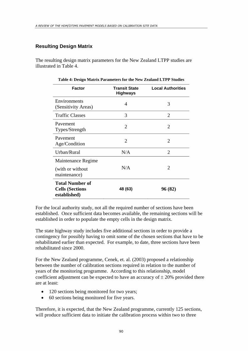
A REVIEW OF THE HDM/DTIMS PAVEMENT MODELS BASED ON CALIBRATION SITE DATA
90
Resulting Design Matrix The resulting design matrix parameters for the New Zealand LTPP studies are illustrated in Table 4.
Table 4: Design Matrix Parameters for the New Zealand LTPP Studies
Factor Transit State Highways
Local Authorities
Environments (Sensitivity Areas) 4 3
Traffic Classes 3 2
Pavement Types/Strength 2 2
Pavement Age/Condition 2 2
Urban/Rural N/A 2
Maintenance Regime
(with or without maintenance)
N/A 2
Total Number of Cells (Sections established)
48 (63) 96 (82)
For the local authority study, not all the required number of sections have been established. Once sufficient data becomes available, the remaining sections will be established in order to populate the empty cells in the design matrix. The state highway study includes five additional sections in order to provide a contingency for possibly having to omit some of the chosen sections that have to be rehabilitated earlier than expected. For example, to date, three sections have been rehabilitated since 2000. For the New Zealand programme, Cenek, et. al. (2003) proposed a relationship between the number of calibration sections required in relation to the number of years of the monitoring programme. According to this relationship, model coefficient adjustment can be expected to have an accuracy of ± 20% provided there are at least:
• 120 sections being monitored for two years; • 60 sections being monitored for five years.
Therefore, it is expected, that the New Zealand programme, currently 125 sections, will produce sufficient data to initiate the calibration process within two to three

Appendix A
91
years of data collection. The duration of the study is undetermined but it is expected to be at least ten years.
Section Selection Criteria It was decided to adopt most of the geometric and condition homogeneity criteria as specified in the HDM-4 Calibration Guidelines (Bennett and Paterson, 2000) and New Zealand Calibration Guidelines (Henning and Riley, 2000). These criteria included:
• avoiding steep gradients; • disallowing sag curves; • excluding sections with major drainage structures; • restricting the total surface thickness.
The major advantage of adopting the above was consistency for the data collection. However, by excluding highway sections according to the above criteria, it is not known whether the resulting models to be developed will be appropriate for these sections.
Data Collection Regime
Survey Accuracy and Intervals Requirements In accordance with the study objectives, the data collection needed to be undertaken with an accuracy that would allow calibration of the models (namely, adjusting calibration coefficients) in the short term as well as providing for adjusting the model format at a later stage. In order to achieve both of these, a number of factors were considered, including:
• The precision output of the various data collection equipment; • The referencing methodology of measurements – to ensure that consecutive
surveys are performed at exactly the same location (within ± 100mm of the original location);
• The expected variation in data due to the change in the physical condition and in conducting the measurements itself.
Ultimately, results from the LTPP study will have to be applied to the network level pavement deterioration which is based on HSD measurements. Therefore, consistency in the approach between the two levels of data collection was imperative. For example, for Transit New Zealand, a standard wheel track spacing (distance between left and right laser beams of 1.75m) is used for all HSD roughness measurements. During the LTPP condition measurements a similar approach had to be followed.
Referencing Method and Section Layout The minimum length of 300m for a LTPP section was based on the requirements for a longitudinal profile analysis (roughness calculation) as specified by Sayers and Karamihas (1996). For New Zealand highways, which have a typical curvilinear

A REVIEW OF THE HDM/DTIMS PAVEMENT MODELS BASED ON CALIBRATION SITE DATA
92
alignment, a longer minimum length would have been impractical, as it would have required compromise on the geometrical requirements mentioned earlier. The 300m sections were divided into 50m subsections similar to the layout used for the Gautrans LTPP study (Rohde, et. al 1998). Both the start and end point of the LTPP sections were indicated with marker posts alongside the road; on the centreline of the road, a steel rod was driven flush with the road surface. In addition, the GPS co-ordinates of these positions were recorded. The combination of methods ensured the exact positioning of the start and end position, should physical marks be lost due to maintenance or resurfacing. Measurement positions were temporarily marked using spray paint on the road surface and the location of these marks was recorded on site layout plans. The photograph in Figure 3 illustrates a typical layout of a LTPP section.
Figure 3: Photo of a LTPP Section on the State Highway
Condition Measurements Once established, the pavement strength and pavement layer composition were determined for all LTPP sections using the FWD and test pits. A sample of the test pit material was subjected to typical soil indicator laboratory tests. On the state highways, FWD surveys are repeated on an annual basis. Annual pavement condition measurements for both LTPP studies in New Zealand are conducted based on an outcome-based contract. Rather than specifying the equipment used for the surveys, the accuracy and the repeatability of the measurement are specified. The methodology used for the various measurements is summarised next. Further details are provided in Transit (2000) and more recently in Henning, et. al. (2004). For the roughness measurements, equipment that met the World Bank Class 1 (Sayers and Karamihas, 1996) and ASTME950 requirements was specified. The contractor responsible for the surveys opted to use the ARRB Walking Profilometer
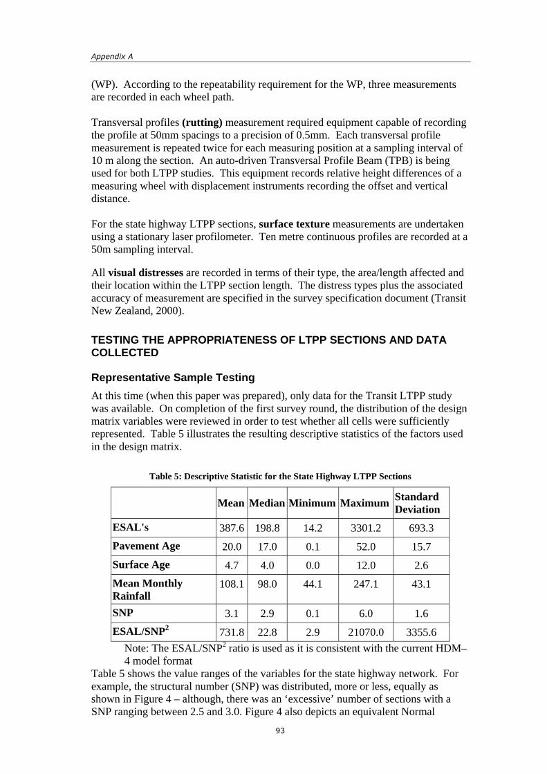
Appendix A
93
(WP). According to the repeatability requirement for the WP, three measurements are recorded in each wheel path. Transversal profiles (rutting) measurement required equipment capable of recording the profile at 50mm spacings to a precision of 0.5mm. Each transversal profile measurement is repeated twice for each measuring position at a sampling interval of 10 m along the section. An auto-driven Transversal Profile Beam (TPB) is being used for both LTPP studies. This equipment records relative height differences of a measuring wheel with displacement instruments recording the offset and vertical distance. For the state highway LTPP sections, surface texture measurements are undertaken using a stationary laser profilometer. Ten metre continuous profiles are recorded at a 50m sampling interval. All visual distresses are recorded in terms of their type, the area/length affected and their location within the LTPP section length. The distress types plus the associated accuracy of measurement are specified in the survey specification document (Transit New Zealand, 2000).
TESTING THE APPROPRIATENESS OF LTPP SECTIONS AND DATA COLLECTED
Representative Sample Testing At this time (when this paper was prepared), only data for the Transit LTPP study was available. On completion of the first survey round, the distribution of the design matrix variables were reviewed in order to test whether all cells were sufficiently represented. Table 5 illustrates the resulting descriptive statistics of the factors used in the design matrix.
Table 5: Descriptive Statistic for the State Highway LTPP Sections
Mean Median Minimum Maximum Standard Deviation
ESAL's 387.6 198.8 14.2 3301.2 693.3 Pavement Age 20.0 17.0 0.1 52.0 15.7 Surface Age 4.7 4.0 0.0 12.0 2.6 Mean Monthly Rainfall
108.1 98.0 44.1 247.1 43.1
SNP 3.1 2.9 0.1 6.0 1.6 ESAL/SNP2 731.8 22.8 2.9 21070.0 3355.6
Note: The ESAL/SNP2 ratio is used as it is consistent with the current HDM–4 model format
Table 5 shows the value ranges of the variables for the state highway network. For example, the structural number (SNP) was distributed, more or less, equally as shown in Figure 4 – although, there was an ‘excessive’ number of sections with a SNP ranging between 2.5 and 3.0. Figure 4 also depicts an equivalent Normal
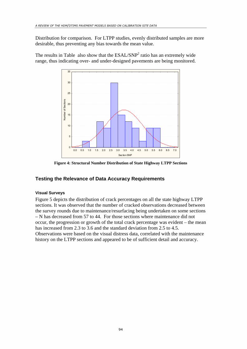
A REVIEW OF THE HDM/DTIMS PAVEMENT MODELS BASED ON CALIBRATION SITE DATA
94
Distribution for comparison. For LTPP studies, evenly distributed samples are more desirable, thus preventing any bias towards the mean value. The results in Table also show that the ESAL/SNP2 ratio has an extremely wide range, thus indicating over- and under-designed pavements are being monitored.
0.0 0.5 1.0 1.5 2.0 2.5 3.0 3.5 4.0 4.5 5.0 5.5 6.0 6.5 7.0
Sec tion SNP
0
5
10
15
20
25
30
35
Num
ber o
f Sec
tions
Figure 4: Structural Number Distribution of State Highway LTPP Sections
Testing the Relevance of Data Accuracy Requirements
Visual Surveys Figure 5 depicts the distribution of crack percentages on all the state highway LTPP sections. It was observed that the number of cracked observations decreased between the survey rounds due to maintenance/resurfacing being undertaken on some sections – N has decreased from 57 to 44. For those sections where maintenance did not occur, the progression or growth of the total crack percentage was evident – the mean has increased from 2.3 to 3.6 and the standard deviation from 2.5 to 4.5. Observations were based on the visual distress data, correlated with the maintenance history on the LTPP sections and appeared to be of sufficient detail and accuracy.

Appendix A
95
Sur vey Round: 1 ACA: N = 57, Mean = 2.29, StdDv = 2.55, Max = 7.98, Min = 0.03Survey Round: 2 ACA: N = 44, Mean = 3.62, StdDv = 4.50, Max = 12.38, Min = 0.04
Cracking Percentage
Perc
ent o
f Obs
erva
tions
Survey Round: 1
0 1 2 3 4 5 6 7 8 9 10 11 12 13 140%
2%
4%
6%
8%
10%
12%
14%
16%
18%
20%
22%
24%
26%
28%
Survey Round: 2
0 1 2 3 4 5 6 7 8 9 10 11 12 13 14
Figure 5: Comparing Crack Status between Survey Rounds (Transit, 2003)
Rutting Measurements Figure 6 illustrates the change of rut values between the two survey rounds. The negative changes shown in rut depth suggests either maintenance has been undertaken or there were measurement errors. The data was interrogated and it was established that the measurements were undertaken within the specified tolerances. Over 70% of the incremental change was less than 0.6 mm compared to the assumed 0.5mm per year - therefore it can be accepted that the rut measurement accuracy specified was appropriate.
0%1%
2%
6%
21%
31%
20%
9%
4%2%
0%1% 1% 0% 0% 0% 0% 0% 0% 0%
-2.50 -1.61 -0. 71 0.18 1.08 1.97 2.86 3.76 4.65 5.55 6.44Incremental Rut Change Between Surv eys (mm)
0
10
20
30
40
50
60
70
80
90
Num
ber o
f 50m
Sub
Sec
tions
Rut change: N = 25 4, Mea n = 0. 13, S tdD v = 0.9 4, Max = 6.4, Mi n = -2.5
Figure 6: Comparing Incremental Rut Change between Survey Rounds (Transit, 2003)
Figure 6 shows the equivalent Normal Distribution of the rut change results. Except for the sections recording ‘extreme’ rut changes over 2mm, the distribution shows Normality. These ‘extreme’ rut change sections required rehabilitation.

A REVIEW OF THE HDM/DTIMS PAVEMENT MODELS BASED ON CALIBRATION SITE DATA
96
Roughness Figure 7 illustrates the incremental change in roughness between the survey rounds. As indicated before some sections have been maintained and there has been an improvement in roughness between the survey rounds. More than 70% of the 100m observations had a roughness change less than ± 0.2 IRI between the survey rounds. This relatively small change in roughness thus warranting the accuracy at which the LTPP sections are surveyed. The average roughness change is slightly negative, implicating an average roughness reduction/improvement. This could be due to either a small bias in the measurements or due to other external factors. Barraclough, et. al. (2003) has indicated that the roughness measurements are sensitive to macro texture – for example some roughness reduction is due to chip embedment. However, this has not been confirmed for the LTPP data.
1%0%0%0%0%0%0%0%0%0%2%
3%
5%
9%
12%
26%
28%
9%
2%1%
0%0%0%0%0%0%0%0%0 %0%
-1.43 -1.17 -0.92 -0.67 -0.41 -0.16 0.10 0.35 0.61 0.86 1.12A nnual Rough ness Chan ge (IR I)
0
10
20
30
40
50
60
70
80
Num
ber o
f 100
m O
bser
vatio
ns
N = 270, Mean = -0.145, StdDv = 0.241, Max = 1.12, Min = -1.43
Figure 7: Comparing Roughness Change between Survey Rounds (Transit, 2003)
Henning, et. al. (2004) also compared these manual measurements with HSD. The conclusion was that the HSD accuracy was reduced due to, amongst other factors, location referencing of the measurements. Variances of these HSD measurements were outside the expected annual deterioration thus reducing the value of the data for calibration purposes.
SUMMARY AND LESSONS LEARNED
The New Zealand LTPP programme consists of two components. The main objective of both these LTPP studies is to monitor the pavement deterioration to an accuracy which will enable the calibration of the World Bank HDM models and, where required, provide sufficient data for model format adjustment. From these objectives, the study layout and data collection regime were developed having undertaken a literature review of relevant international LTPP studies.

Appendix A
97
The Transit New Zealand study, which commenced in 2001, is monitoring 63 sections on the national state highway network. For these sections, data from the two survey rounds, 2001/02 and 2002/03 was presented. The road controlling authority LTPP study has 82 sections, which have been established across 21 road authorities networks including urban and rural sections. The first survey on these sections commenced in November 2003. A literature review of international studies was undertaken to assist the setting up of the design matrix and methodological approach for the New Zealand LTPP studies. The international studies reviewed were:
• HDM-III studies in Brazil; • SHRP studies in the USA and Canada; • ISOHDM calibration studies in countries such as Australia and South Africa.
The literature review of international LTPP was valuable for the development of the scope, goals and objectives during the initial stages of the New Zealand programme. It assisted in highlighting factors to be considered. For example, a decision was required, whether to monitor specially constructed pavements or to limit the study to in-service pavements. It was decided to focus the New Zealand LTPP studies on the pavement performance of typical roads existing on the network, that is to study only in-service pavements taking into account normal maintenance and limited maintenance regimes. Furthermore, the literature review was useful in determining the design matrix, site layout and data collection regime on these pavements. Some of the aspects, which were of particular importance for use on the New Zealand LTPP programme were given in Table 2 earlier. The design matrix developed for the New Zealand programme included factors such as environment, traffic, pavement type/strength, pavement condition/age, network type and maintenance regime. The New Zealand LTPP programme has highlighted the importance of the following:
• If pavement strength or composition is used as a factor in the design matrix, it must be categorised according to the design loading it is expected to carry. This will ensure that the study includes pavements which are under- or over-designed;
• Regional classification should not only include climate or rainfall factors but should also include the impact of the climate on the regional geological make-up. For this programme, a ratio between the subgrade strength and a moisture indicator was used;
• Considering pavements of different ages, reduces the time required for the study. However, the pavement age should be considered in combination with condition data. For example, pavement showing deterioration at an early age must be included with some equally aged pavements without any distresses visible;
• Normally, not all the data are available during the initial establishment of the sections. The New Zealand LTPP programme adopted an incremental establishment of sites where say 80% of the sections were established prior to the first survey round. Following this, the remaining sections are being established to cover gaps in the design matrix.

A REVIEW OF THE HDM/DTIMS PAVEMENT MODELS BASED ON CALIBRATION SITE DATA
98
In defining the data collection regime, the HDM calibration guidelines (Bennett and Paterson, 2000) and the Gautrans study (Rohde, et. al, 1998) suggested that HSD type data is sufficient only for adjusting the model calibration coefficients. If the model formats need adjustment, then higher precision data would be required. Henning, et. al. (2004) demonstrated that referencing (location of the data measurements) significantly contributes to the variance in the results – this applies particularly to HSD. Hence, the New Zealand LTPP studies recommended manual measurement as it was intended to adjust the model formats if required. A review of the data collection regime indicates that it is at an appropriate level for the New Zealand studies. For example 70% of the incremental rutting change was less than 0.6 mm compared to the assumed 0.5mm per year. Similarly, more than 70% of the 100m observations had a roughness change of less than 0.2 IRI between the survey rounds. This study has demonstrated the importance of aligning data collection regimes with the study outcome and with current data collection regimes on a network level. At this early stage, the LTPP New Zealand programme has been successful in achieving its goals and objectives. On the other hand, a review of the data has highlighted areas where further research is required and proceeding – for example in determining the factors contributing to the annual condition change and actual deterioration compared to recorded characteristics. The next major stage of the programme is to investigate the model format and determine the calibration requirements.

Appendix A
99
REFERENCES Barraclough, B., Brown, D.N., And Henning, T.F.P. 2002 Calibration and Validation
Report. MWH New Zealand, Wellington, New Zealand. Bennett, C.R. Paterson, W.D.O. (2000) A Guide to the Calibration and Adaptation.
HDM - 4. Volume 5. The Highway Development and Management Series. PIARC
Benson, P. (1991) Biases and Gaps in the GPS database. Paper delivered at the
Proceedings of SHRP midcourse Assessment, Guide No. SHRP-LTPP-UWP-91-514. Strategic Highway Research Programmes, National Research. USA
Cenek, P.D. (2001). Summary Report- Regionalisation of Roading Authorities for
Pavement Deterioration Modelling. Memorandum to Ken Hudson, Opus Central Laboratories, Lower Hutt, NZ.
Cenek, P.D. (2003). Experimental Design for Determining Calibration Coefficients
for HDM-III Field Deterioration Models incorporated in RIMS dTIMS. Opus Central Laboratories, Lower Hutt, NZ.
FHWA, (2000). LTPP Product Plan. Publication No. FHA-RD-01-086. US
Department of Transportation. Federal Highway Administration. USA. GEIPOT (Ministerio Dos Transportes), UNDP (United Nations Development
Programme), (1981) Research on Interrelationships Between Cost of Highway Construction, Maintenance and Utilisation. Final Report. Volume 2 – Methods and Organization. Brazilia
Henning, T.F.P. Hart, G. (2000) Calibration Sites for Pavement Deterioration
Modelling. Transit Operational Policy Document. Asset Management Team. Transit New Zealand, Wellington, New Zealand.
Henning, T.F.P. Costello, S.B. Dunn, R.C.M. Parkman, C.C. and Hart, G. (2004) The
Establishment of A Long-Term Pavement Performance Study on The New Zealand State Highway Network. Accepted for publication in the ARRB Journal.
Henning, T.F.P. Riley,M. (2000) Calibration Guidelines for Pavement Deterioration
Models and Work Effects Models in dTIMS. HTC Infrastructure Management. Auckland.
Martin, T. (1994). Pavement Behaviour Prediction for Life-cycle Costing. Research
Report ARR No. 255. Australian Road Research Board Ltd. Victoria, Australia.
Martin, T. (2003). Pavement Performance Prediction Deterioration Model
Development - Data Review and Calibration of HDM-4 Road Deterioration Models. Research Report RC 2051. Australian Road Research Board Ltd. Victoria, Australia.

A REVIEW OF THE HDM/DTIMS PAVEMENT MODELS BASED ON CALIBRATION SITE DATA
100
Paterson, W.D.O. (1987) Road Deterioration and Maintenance Effect Models for Planning and Maintenance. World Bank Publications. Washington DC. USA
Rohde, G.T, Jooste, F, Sadzik, ES and Henning, TFP, (1998). “The Calibration and
Use of HDM-4 Performance Models in a Pavement Management System”. 4th International Conference on Managing Pavements. ICC Durban, ISBN: 0-620-22378-2.
Rohde, G.T. Wolmerans, I and Sadzik, E.S. (2002). The calibration and Validation of
HDM Performance Models in the Gauteng PMS. 21st Annual South African Transport Conference, CSIR, South Africa.
Sayers, A.W. and Karamihas, S.M. (1996). Measuring and Analyzing Road Profiles.
Short Course. The University of Michigan Transportation Research Institute. USA
SHRP-LTPP, (1990). Guide for Field Materials Sampling, Handling and Testing.
Operational Guide No. SHRP-LTPP-OM-006. Strategic Highway Research Programmes, National Research, USA
SHRP-LTPP, (1999). Introduction to LTPP Data. Strategic Highway Research
Programmes, National Research Council, USA Thornthwaite, C. W. (1954). Estimating Soil Tractionability from Climatic Data. Centerton, N.J. Johns Hopkins University, Laboratory of Climatology. Transit New Zealand, (2000). Calibration Sections Survey, Contract Number SM3-
688/P6/10 Transit New Zealand, Wellington, NZ Transit New Zealand, (2003). Calibration of Pavement Deterioration Models Based
on the 2003 Calibration Data, Transit New Zealand, Wellington, NZ Tepper, S. Martin. T. (1999) Long-term Pavement Performance Maintenance
(LTPPM) – Progress Report. Report RC90268-1. For Austroads. ARRB Transportation Research Ltd. Melbourne, Australia.
Weinert, H.H. (1974). A climatic Index of Weathering and its Application in Road
Construction. Geotechnique, Vol. 24, Pretoria, SA.