Research and Development at U.S. Research Universities:

An Analysis of Scope Economies

by

Kwansoo Kim

Bradford Barham

Jean-Paul Chavas

and

Jeremy Foltz *

Abstract: This work investigates the presence and sources of economies of scope in R&D at U.S. research universities. The analysis evaluates the tradeoffs and synergies arising between traditional university research outputs (articles and doctorates) and academic patents. We propose a new measure of economies of scope based on a primal representation of the underlying technology. We derive a decomposition of economies of scope which identifies its sources (e.g., complementarity effects and scale effects). Non-parametric estimates of scope economies using R&D input and output data from 92 research universities show significant economies of scope between articles and patents, but modest complementarities. (JEL O3, O31, O33, C6, L31)

Keywords: R&D, university, patent, scope, complementarity, scale.

* Kwansoo Kim is Assistant Professor, Seoul National University, Seoul, Korea; Bradford

Barham, Jean-Paul Chavas and Jeremy Foltz are respectively Professor, Professor, and Assistant

Professor, University of Wisconsin, Taylor Hall, Madison, WI 53706. Senior authorship is

equally shared. Correspondence should be sent to jdfoltz@wisc.edu.

1

Research and Development at U.S. Research Universities: An Analysis of Scope Economies

This work investigates the presence and sources of economies of scope in R&D at U.S. research

universities. The analysis evaluates the tradeoffs and synergies arising between traditional

university research outputs (articles and doctorates) and academic patents. We propose a new

measure of economies of scope based on a primal representation of the underlying technology.

We derive a decomposition of economies of scope which identifies its sources (e.g.,

complementarity effects and scale effects). Non-parametric estimates of scope economies using

R&D input and output data from 92 research universities show significant economies of scope

between articles and patents, but modest complementarities. (JEL O3, O31, O33, C6, L31)

Research and development (R&D) are fundamental to technological progress and

economic growth. Because universities are dedicated to the production and dissemination of new

knowledge and new technologies, university spillovers and their effects on economic growth

have been the subject of much interest (e.g., Adam Jaffe, 1989; Rebecca Henderson et al., 1998;

Bronwyn H. Hall et al., 2003b; Lee Branstetter, 2003; Suzanne Scotchmer, 2004). In the early

1980s, changes in federal policies, starting with the Bayh-Dole Act, made it easier for U.S.

universities to retain the property rights to inventions obtained from federally funded research.

This broad institutional change in intellectual property rights, combined with recent tightening in

state and federal budgets, have helped to increase university efforts to secure both research

sponsorship and intellectual property right royalties from the private sector.

Over the last ten years, academic patenting in the U.S. has increased sharply (Jeremy D.

Foltz et al., 2005). University tech transfer offices, many recently established, intensified their

1

efforts to secure property rights to new knowledge and to transfer their research findings to the

private sector through licensing arrangements, start-ups, and other remunerative arrangements.

These efforts have raised a wide range of questions about the changing role of public and private

research universities in the economy, society, and the pursuit of knowledge (e.g., Pierre Azoulay

et al., 2004; Lee Branstetter, 2003; Bronwyn H. Hall et al., 2003b; Rebecca Henderson et al.,

1998; Richard A. Jensen and Marie C. Thursby, 2001; Bhaven Sampat et al., 2003). One key

issue is the existence of possible synergies between patenting and more traditional university

outputs; i.e. the existence and nature of economies of scope within research universities.

Following the pioneering work by William J. Baumol et al. (1982), economies of scope

measure the benefit for a firm to produce multiple outputs. Measuring such benefits for

universities has provided useful insights into their organizational structure (e.g., Elchanan Cohn,

et al., 1989; Hans De Groot et al., 1991; G. Thomas Sav, 2004). But, does the diversification of

research universities into patenting activities generate significant synergies? In principle,

university patenting and private-public partnering activities can help research universities

become more effective in stimulating innovations (e.g., Hall et al., 2003b). However, at this

point, the nature and magnitude of these benefits remain unclear. How large are these benefits?

And how are they distributed among universities of different sizes or different types (e.g., private

versus public universities)?

This paper investigates the presence and sources of economies of scope in R&D

production at U.S. research universities. The analysis addresses the following issue in the

literature on academic patenting: whether synergies arise between traditional university research

outputs (articles and doctorates) and the more recent and burgeoning output of academic patents.

Framing the empirical analysis requires a theoretical exposition of the concept of economies of

2

scope that deepens our understanding of this phenomenon in ways that are relevant not only to

R&D processes but also to the many other economic contexts where scope economies may arise.

Overall, our paper makes three methodological contributions.

First, the conventional approach to measuring economies of scope typically involves

analyzing complete specialization among outputs (see Baumol et al., 1982). This is relevant in

the evaluation of mergers and acquisitions when firms are deciding on whether to produce jointly

distinctive outputs or to spin off separate operations. However, universities are rarely completely

specialized. On that basis, we develop an analysis that allows for partial specialization between

production processes. Allowing for partial specialization permits a search for economies of scope

across a more nuanced range of possible outcomes than is typically depicted in previous

economies of scope studies.

The second methodological contribution of this paper is to develop and apply a primal

approach to economies of scope. The approach relies on David G. Luenberger’s (1995) shortage

function as a representation of the underlying technology. This primal approach is especially

useful in measuring scope economies in contexts where input cost data are difficult to obtain or

fraught with measurement problems, such as in our empirical study with respect to certain input

prices that shape university research and teaching outputs.

The third and perhaps most far-reaching contribution of this paper is its decomposition of

economies of scope into three measures: complementarities between outputs, economies of scale

in multiple outputs (along different degrees of specialization), and a convexity component. This

decomposition provides a clear picture of the basis for scope economy outcomes in production of

multiple outputs, because it permits identification of whether the scale of operation and/or the

complementarity of outputs are driving scope benefits. This decomposition extends the

3

contributions of Paul Milgrom and John Roberts (1990) by making identification of

complementarity and other sources of scope economies both more tractable and intuitive. Our

empirical analysis of U.S. research universities illustrates how both scale and complementarity

can drive scope outcomes for economic entities as their size and type change.

Finally, our scope analysis is applied to U.S. research universities. This provides

evidence on the synergies that exist between patenting and more traditional academic research

outputs. R&D input and output data from 92 top-tier U.S. research universities are used to

estimate economies of scope for public and private universities of different sizes. The estimates

are obtained using a non-parametric representation of the underlying technology, and control for

quality of article and patent outputs. The empirical results show that significant variations exist

in the magnitude and sources of economies of scope across U.S. universities. Indeed, while scope

economies are evident in most of the sample, evidence for strong complementarity among these

research activities is more limited.

The organization of the paper is as follows. Section 2 provides the basic model and a

characterization of firms going from integrated, to mildly specialized, to fully specialized output

choices. Section 3 proposes a new primal measure of scope economies based on Luenberger’s

(1995) shortage function. Section 4 presents a decomposition of scope economies which

identifies the potential sources of scope benefits among outputs. Section 5 discusses the dataset

on university research outputs and inputs. Using a non-parametric approach, section 6 applies

our proposed methodology to estimate scope economies and their sources across a spectrum of

specialization for U.S. research universities. Section 7 reports the empirical results, and section 8

concludes.

4

I. The Model

Consider a firm facing a production process producing m outputs using n inputs, where y

= (y1, …, ym) ∈ R m+ is the vector of outputs, and x ∈ R n

+ is the vector of inputs. Using the netput

notation (where inputs are negative and outputs are positive), the netputs are z ≡ (-x, y). The

technology is represented by the production possibility set F ⊂ R n− ×R m

+ , where z ≡ (-x, y) ∈ F

means that outputs y can be produced from inputs x. Throughout the paper, we assume that the

set F is closed and with a non-empty interior. We want to investigate under what conditions the

multiproduct firm would gain (or lose) from reorganizing its production activities in a more

specialized way. The reorganization involves breaking up the firm into K specialized firms, 2 ≤

K ≤ m. Given the output index I = {1, …, m}, consider its partition I = {IA1, IA2, …, IAK, IB},

where IA = {IA1, IA2, …, IAK}, IAk being the set of outputs that the k-th firm is specializing in, k =

1, …, K, while IB being the set of outputs that no particular firm specializes in. Let yk = (y1k, …,

ymk) denote the outputs produced by the k-th specialized firm, k = 1, …, K.

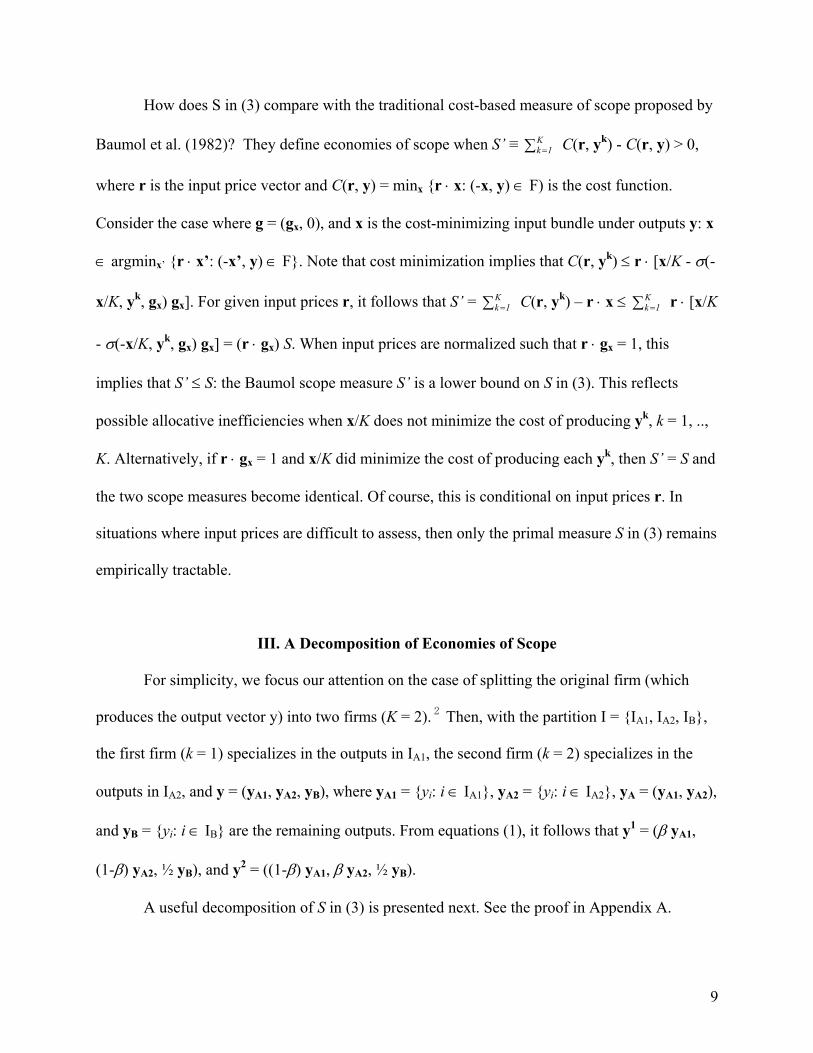
Our analysis of the economics of specialization has two objectives in mind. First, we

explore what happens under alternative specialization schemes holding total output constant.

This requires selecting the outputs of specialized firms such that ∑ K1k= yk = y, where the K

specialized firms produce the same aggregate output vector y as the original firm. Second, we

want to allow various degrees of specialization, going from “mild specialization” to “complete

specialization”. In this context, given y = (y1, …, ym), consider the following patterns of

specialization for the k-th firm

(1a) yik = β yi, if i ∈ IAk,

(1b) = yi (1-β)/(K-1), if i ∈ IAk’, k’ ≠ k,

(1c) = yi/K, if i ∈ IB,

5

for some β, 1/K < β ≤ 1, k = 1, …, K. This represents a reorganization of the original firm into K

firms toward greater specialization, where the k-th firm becomes more specialized in the

production of outputs in the sets IAk, k = 1, …, K.

Note that the specification (1a)-(1c) always satisfies ∑ K1k= yi

k = yi, i = 1, …, m. This

guarantees that the same aggregate outputs are being produced before and after the firm

reorganization. The parameter β in (1a) represents the proportion of the original outputs {yi: i ∈

IAk} produced by the k-th firm. And from (1b), (1-β) represents the proportion of the original

outputs {yi: i ∈ IAk’, k’ ≠ k} produced by the k-th firm. When β = 1, this means that the k-th firm

produces the same quantities {yi: i ∈ IAk} as the original firm and that such outputs are produced

only by the k-th firm. In this case, the k-th firm is completely specialized in the production of the

outputs in the set IAk (and it produces none of the other outputs in the sets IA). Alternatively,

when 1/K < β < 1, we allow for partial specialization. For example, if K = 2 and β = 0.9, then the

first firm (corresponding to k = 1) produces 90% of the quantities {yi: i ∈ IA1} produced by the

original firm, while the second firm (corresponding to k = 2) produces the remaining 10%. And

the second firm (k = 2) produces 90% of the quantities {yi: i ∈ IA2} produced by the original

firm, while the first firm (k = 1) produces the remaining 10%. Finally, note that (1c) allocates the

outputs in the set IB equally among the K specialized firms. This simply reflects that the outputs

in IB are not involved in the patterns of specialization as the firm reorganizes.

Equations (1a)-(1c) include as a special case the situation where β = 1 and IB = ∅. This

is the case of complete specialization (e.g., as investigated by Baumol et al., 1982 based on a cost

function). As such, our approach extends previous analyses in two directions. First it allows for

specialization in a subset of outputs (when IB ≠ ∅). This can become relevant in the economics

of specialization when 2 ≤ K < m, i.e., when the number of specialized firms is less than the

6

number of outputs. Second, as noted above, it allows for partial specialization in the outputs of

the set IA (with 1/K < β < 1). This is relevant when the K firms want to explore the economics of

becoming more specialized (thus deemphasizing the production of some of their outputs) but

without a complete shutdown of some of their production lines.

II. Economies of Scope

To investigate the economics of specialization, we need to rely on measures that can be

meaningfully added across firms. This is the case of the cost function which has provided the

standard basis for measuring economies of scope. In this context, Baumol et al. (1982) have

defined economies of scope (diseconomies of scope) as situations where it is less costly (more

costly) to produce the aggregate outputs y from an integrated firm as compared to specialized

firms. This has stimulated empirical analyses of the benefit (or cost) of producing from an

integrated multi-output firm. However, the cost function requires that all inputs be market goods

with observable prices. There are situations where some inputs have prices that are not

observable or that do not reflect their marginal contribution to the production process. An

example in higher education includes Ph.D. students: their cost to a university can differ

significantly from their marginal contribution to university research productivity. Under such

scenarios, the use of the cost function becomes problematic. But under the convexity assumption,

it is well known that the cost function is dual to the underlying technology. This means that there

are alternative ways of measuring economies of scope directly from the production technology.

Like the cost function, this requires using a measurement of the production technology that can

be meaningfully added across firms. A measurement that satisfies this property is Luenberger’s

7

shortage function, which we use below in our analysis of the scope economies associated with

integrated production.

Following Luenberger (1995), letting g ∈ R mn++ -{0} be some reference netput bundle,

define the shortage function:

(2) σ(z, g) = minγ {γ : (z - γ g) ∈ F} if (z - γ g) ∈ F for some scalar γ,

= +∞ otherwise.

The shortage function σ(z, g) in (2) measures how far the point z is from the frontier of

technology, expressed in units of the reference bundle g. To illustrate, consider the case where g

= (0, …, 0, 1). Then, the shortage function is σ(z, g) = minγ {γ: (z1, …, zm-1, zm - γ) ∈ F} = zm -

f(z1, …, zm-1), where f(z1, …, zm-1) is a (multi-output) production frontier, and feasibility implies

that zm ≤ f(z1, …, zm-1). Under differentiability, this implies that ∂σ/∂zi = -∂f/∂zi, i.e. that the

marginal shortage ∂σ/∂zi is the negative of the marginal product ∂f/∂zi with respect to the i-th

netput, i = 1, …, m-1. Note that, given a reference bundle g, the shortage function can be

meaningfully added across firms. As such, the shortage function provides a convenient basis for

analyzing scope issues and the benefit/cost of specialization.１

Starting from a firm using netputs z ≡ (-x, y), we analyze whether there are any benefits

from reorganizing its production activities according to equation (1), where yk ∈ R m+ is produced

by the k-th specialized firm, k = 1, …, K, with y = ∑ =K

1k yk. If the k-th firm uses inputs xk, the

shortage function associated with (-xk, yk) is σ(-xk, yk, g). In a way similar to (1c), consider the

case where inputs x are equally divided between the K firms, with xk = x/K, k = 1, …, K.

Definition 1: Given equations (1), economies of scope (diseconomies of scope) with respect to

the partition I = {IA1, …, IAK, IB} in the production of outputs y are said to exist if

8

(3) S(β, IA1, …, IAK, IB, z, g) ≡ ∑ =Κ

1k σ(-x/K, yk, g) - σ(z, g) > (<) 0,

Note that ∑ =K

1k σ(-x/K, yk, g) can be interpreted as the smallest distance to the

technology frontier (as measured by the number of units of the reference bundle g) when the

aggregate netputs z = (-x, y) are produced by K specialized firms: (-x/K, yk), k = 1, …, K. Thus,

equation (3) compares the distance to the technology frontier producing y from an integrated

firm versus specialized firms.

To help interpret (3), consider the case where netputs are market goods with prices p ∈

R mn+++ . Then, starting from the aggregate netput z and under technical efficiency, πa = p ⋅ [z - σ(-

x, y, g) g] is the profit for the integrated firm, while πs = p ⋅ [ ∑ =K

1k zk - σ(-x/K, yk, g) g] is the

aggregate profit for the K specialized firms, where zk = (-x/K, yk), and yk satisfies (1), k = 1, …,

K. It follows that the difference in profit is

πa - πs = [ ∑ =K

1k σ(-x/K, yk, g) - σ(-x, y, g)] p ⋅ g,

where (πa - πs) measures the benefit of integrated production in a multiproduct firm. When

positive, this difference reflects positive synergy among outputs. Given p ⋅ g > 0, this makes it

clear that S(β, IA1, …, IAK, IB, z, g) > 0 in (3) corresponds to economies of scope, identifying the

presence of synergies or positive externalities in the production process among the outputs in IAk,

k = 1, …, K. Alternatively, diseconomies of scope exist (with S(β, IA1, …, IAK, IB, z, g) < 0) if

producing netputs z from an integrated firm (as opposed to K specialized firms) reduces the

benefits. This identifies the presence of negative externalities in the production process among

the outputs in IAk, k = 1, …, K.

9

How does S in (3) compare with the traditional cost-based measure of scope proposed by

Baumol et al. (1982)? They define economies of scope when S’ ≡ ∑ =K

1k C(r, yk) - C(r, y) > 0,

where r is the input price vector and C(r, y) = minx {r ⋅ x: (-x, y) ∈ F) is the cost function.

Consider the case where g = (gx, 0), and x is the cost-minimizing input bundle under outputs y: x

∈ argminx’ {r ⋅ x’: (-x’, y) ∈ F}. Note that cost minimization implies that C(r, yk) ≤ r ⋅ [x/K - σ(-

x/K, yk, gx) gx]. For given input prices r, it follows that S’ = ∑ =K

1k C(r, yk) – r ⋅ x ≤ ∑ =K

1k r ⋅ [x/K

- σ(-x/K, yk, gx) gx] = (r ⋅ gx) S. When input prices are normalized such that r ⋅ gx = 1, this

implies that S’ ≤ S: the Baumol scope measure S’ is a lower bound on S in (3). This reflects

possible allocative inefficiencies when x/K does not minimize the cost of producing yk, k = 1, ..,

K. Alternatively, if r ⋅ gx = 1 and x/K did minimize the cost of producing each yk, then S’ = S and

the two scope measures become identical. Of course, this is conditional on input prices r. In

situations where input prices are difficult to assess, then only the primal measure S in (3) remains

empirically tractable.

III. A Decomposition of Economies of Scope

For simplicity, we focus our attention on the case of splitting the original firm (which

produces the output vector y) into two firms (K = 2).２ Then, with the partition I = {IA1, IA2, IB},

the first firm (k = 1) specializes in the outputs in IA1, the second firm (k = 2) specializes in the

outputs in IA2, and y = (yA1, yA2, yB), where yA1 = {yi: i ∈ IA1}, yA2 = {yi: i ∈ IA2}, yA = (yA1, yA2),

and yB = {yi: i ∈ IB} are the remaining outputs. From equations (1), it follows that y1 = (β yA1,

(1-β) yA2, ½ yB), and y2 = ((1-β) yA1, β yA2, ½ yB).

A useful decomposition of S in (3) is presented next. See the proof in Appendix A.

10

Proposition 1: Assume that the shortage function σ(z, g) is continuous in z and differentiable

almost everywhere in y ∈ R m+ . Under equations (1) with K = 2, there are economies of scope in

the production of outputs y = (yA1, yA2, yB) ∈ R m++ if and only if

S(β, IA1, IA2, IB, z, g) ≡ SC(β, IA1, IA2, IB, z, g) + SR(β, IA1, IA2, IB, z, g)

(4) + SV(β, IA1, IA2, IB, z, g) > 0,

where

SC(β, IA1, IA2, IB, z, g) ≡ - ∫ −

A2

A2

y β

y β)(1[∂σ/∂γ(-½ x, β yA1, γ, ½ yB, g)

(5a) - ∂σ/∂γ(-½ x, (1-β) yA1, γ, ½ yB, g)] dγ,

(5b) SR(β, IA1, IA2, IB, z, g) ≡ 2 σ(½ z, g) - σ(z, g),

SV(β, IA1, IA2, IB, z, g) ≡ σ(-½ x, β yA, ½ yB, g) + σ(-½ x, (1-β) yA, ½ yB, g)

(5c) - 2 σ(½ z, g).

Proposition 1 gives a necessary and sufficient condition for economies of scope in the

production of outputs y. Equation (4) decomposes the scope measure S(β, IA1, IA2, IB, z, g) in (3)

into three additive terms: SC(β, IA1, IA2, IB, z, g) given in (5a), SR(β, IA1, IA2, IB, z, g) given in

(5b), and SV(β, IA1, IA2, IB, z, g) given in (5c).

The term SC in (5a) depends on how yA1 affects the marginal shortage of yA2. As

illustrated in section 3, marginal shortage can be interpreted as the negative of the marginal

product. With this interpretation in mind, given β ∈ (0.5, 1], we define complementarities

between yA1 and yA2 at point y as any situation where the shortage function σ(z, g) satisfies

[∂σ/∂yA2(-½ x, β yA1, γ yA2, ½ yB, g) - ∂σ/∂yA2 (-½ x, (1-β) yA1, γ yA2, ½ yB, g)] ≤ 0 for all γ ∈ [0,

1], with the inequality being strict over a set of nonzero measure. Then, it is clear from (5a) that

11

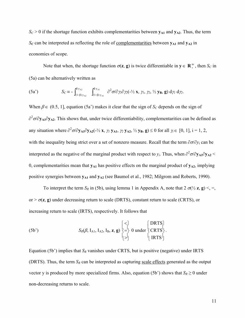
SC > 0 if the shortage function exhibits complementarities between yA1 and yA2. Thus, the term

SC can be interpreted as reflecting the role of complementarities between yA1 and yA2 in

economies of scope.

Note that when, the shortage function σ(z, g) is twice differentiable in y ∈ R m+ , then SC in

(5a) can be alternatively written as

(5a’) SC ≡ - ∫ −

A2

A2

y β

y β)(1 ∫ −

A1

A1

y β

y β)(1∂2σ/∂γ1∂γ2(-½ x, γ1, γ2, ½ yB, g) dγ1 dγ2.

When β ∈ (0.5, 1], equation (5a’) makes it clear that the sign of SC depends on the sign of

∂2σ/∂yA1∂yA2. This shows that, under twice differentiability, complementarities can be defined as

any situation where ∂2σ/∂yA1∂yA2(-½ x, γ1 yA1, γ2 yA2, ½ yB, g) ≤ 0 for all γi ∈ [0, 1], i = 1, 2,

with the inequality being strict over a set of nonzero measure. Recall that the term ∂σ/∂yi can be

interpreted as the negative of the marginal product with respect to yi. Thus, when ∂2σ/∂yA1∂yA2 <

0, complementarities mean that yA1 has positive effects on the marginal product of yA2, implying

positive synergies between yA1 and yA2 (see Baumol et al., 1982; Milgrom and Roberts, 1990).

To interpret the term SR in (5b), using lemma 1 in Appendix A, note that 2 σ(½ z, g) <, =,

or > σ(z, g) under decreasing return to scale (DRTS), constant return to scale (CRTS), or

increasing return to scale (IRTS), respectively. It follows that

(5b’) SR(β, IA1, IA2, IB, z, g)

>=<

0 under

IRTSCRTSDRTS

.

Equation (5b’) implies that SR vanishes under CRTS, but is positive (negative) under IRTS

(DRTS). Thus, the term SR can be interpreted as capturing scale effects generated as the output

vector y is produced by more specialized firms. Also, equation (5b’) shows that SR ≥ 0 under

non-decreasing returns to scale.

12

Finally, the term SV(β, IA1, IA2, IB, z, g) in (5c) reflects the effect of convexity. From

lemma 2 in Appendix A, if the technology F is convex, the shortage function σ(z, g) is convex in

z and satisfies σ(θ z + (1-θ) z’, g) ≤ θ σ(z, g) + (1-θ) σ(z’, g) for any θ ∈ [0, 1] and any z and z’.

Choosing θ = ½, it follows that SV(β, IA1, IA2, IB, z, g) ≥ 0 under a convex technology. In other

words, a convex technology is sufficient to imply that SV ≥ 0. In addition, note that SV = 0 when β

= 0.5. Thus, under a convex technology, one can expect SV to increase with the degree of

specialization β ∈ [0.5, 1].

The decomposition provided in Proposition 1 indicates that there can be multiple sources

of economies of scope. Identifying the role played by each source appears useful as it can

provide useful insights into the economics of specialization. This is illustrated next in an

application to U.S. universities.

IV. Data

The dataset combines information on research inputs and outputs in the sciences and

engineering for 92 US universities, including 61 public universities and 31 private universities

for the period of 1995-1998. This dataset contains for all 92 universities the following data:

1) Total patent counts and patent citations from all science and engineering fields (U.S.

Patent Office, 2004; and Hall et al., 2003a),

2) Article counts and citations from all science and engineering fields (ISI Web of

Science, 2004),

3) Total number of doctorates and bachelor degrees granted in the sciences as well as the

number of graduate students, faculty, and post-docs (National Science Foundation, 2004).

13

Further details on the sources of the data and key choices in the construction of the

dataset can be found in Appendix B. One key aspect of the dataset warrants discussion here. The

dataset focuses on scientific inputs and outputs, reflecting our interest in studying economies of

scope between university research and university patents. Thus, our measures of scientific inputs

and outputs are appropriate to investigate the possible tradeoff that exists between university

research outputs and university patents (which are almost entirely produced by the sciences).

In order to proceed with the empirical analysis, we need a representation of the university

production process. In the case of student training, we measure undergraduate bachelor’s degrees

in the sciences as university outputs. However, graduate students can be both inputs and outputs:

they are outputs of the university educational function; but they are also inputs into the research

process (especially through their theses and dissertations). To account for this dual function of

graduate students, we assume that they are outputs, except in their final year when they are

treated as inputs into the university research process. Since there is typically a one or two year

delay between when research takes form as an article or patent and when a graduate student

worked on it, we think that our assumption is a reasonable match with the output data we have.

Thus, we measure continuing graduate students as outputs, and PhD’s granted as inputs. In this

context, universities are involved in the production of four outputs (journal articles, patents,

trained undergraduate students, and trained graduate students) using three inputs (faculty, post-

doctoral researchers, and PhD graduate students).

To account for quality differentials, quality adjustments are made on university output

measures of patents and articles as well as input measure of faculty. Quality-adjusted output

measures are obtained, where citations of articles and patents are used to control for quality of

those two research outputs. Quality-adjusted input measure for faculty is obtained by multiplying

14

total faculty numbers and the university’s average faculty salary (National Science Foundation,

2004). Science patent assignee and citation information were obtained from the NBER patent

database (Hall et al., 2003a), while the Science Citation Index (ISI Web of Science, 2004)

provided the science article and citation counts by year for each university. Patents are credited

by application year rather than by grant date in order to measure them as close as possible to the

date research efforts occurred. Quality adjustments were sought because in the case of research

output, quality is likely to matter significantly to the implicit value of the research and also to the

potential synergies between patents and articles. In the first case, highly cited articles and patents

are likely to generate flows of additional research or licensing funds to the author or assignee,

while in the latter research that gives rise, for example, to an article that is highly cited may also

be more likely to generate a patent than would a larger number of un-cited articles. Empirically,

studies of patent citations have shown that they provide a reasonable proxy for both the quality

of a patent and knowledge spillovers from patents, because each time a new patent uses a piece

of research from another patent it is obligated to cite the previous patent (Henderson et al.,

1998). Article citations are also commonly used as measures of quality in studies of departmental

or university quality (e.g., Amy Adams, 1998).

Using citations as a quality measure requires attending to the time dependency of the

counts, namely the truncation problem associated with more recent articles or patents that may

not have had time to generate many citations (Sampat et al., 2003). The quality adjustment

measure used for each life science article/patent is the deviation from the average citation rate of

an article/patent in the same broad class/category published in the same year. For example, a

1995 biochemistry article with 10 citations is compared to the average level of citations of all

biochemistry articles produced in that year. For a given year, the average article within a

15

category has a citation rate of 1, with higher quality articles then having a measure greater than

one and lower quality articles receiving a measure between zero and one. This relative citation

approach minimizes a truncation bias that would be introduced by using an absolute citation

count. Further details on the citation measure are provided in Appendix B.

Finally, we account for the fact that the production process for universities is dynamic:

the process of scientific discovery is typically time-consuming. For example, lagged inputs can

affect current outputs in the presence of production lags (e.g., it takes time for research to be

published). And lagged outputs may affect current outputs in the presence of temporal synergies

in production. This implies a need to incorporate dynamics in the representation of the

underlying technology. This is done by specifying and estimating a multi-period production

technology over a four-year period. Outputs for the current year are assumed to depend on inputs

of the current year, but also on inputs and outputs from the three previous years. The effects of

lagged quantities are captured by a weighted average of the corresponding quantities, with

weight equal to 0.5 for lag one-year, 0.37 for lag two-years, and 0.13 for lag three-years. As a

result, our dynamic production process is represented by eight outputs (four current outputs and

four lagged outputs) and six inputs (three current inputs, and three lagged inputs). Our empirical

investigation of economies of scope between university research outcomes (patents and articles)

relies on data for 1995-1998 (the most recent years with complete data available).

V. Empirical Analysis

The shortage function described in equation (2) provides a generic representation of the

frontier of technology. It can be estimated either using parametric methods (involving a

parametric specification followed by an econometric estimation of the parameters) or non-

16

parametric methods. Below, we rely on a non-parametric approach for several reasons. First, it

provides a flexible representation of the multi-output production frontier. Second, it does not

require imposing a parametric structure on the problem. Third, when the number of netputs is

large, it is not subject to collinearity problems. Finally, it does not require that each data point be

on the frontier technology, which allows for possible technical inefficiencies (see Foltz et al.,

2005).

Thus, we use input and output data to recover an estimate of the underlying multi-output

production technology for universities. Again, this is done by representing the dynamic process

of producing outputs (research articles, patents, undergraduate degrees granted, and graduate

students (excluding final-year doctorates)) using a set of inputs (post-docs, doctorates in their

final year of study, and faculty). And using the shortage function in (2), we have measurements

of how far is each point from the production frontier.

Next, a nonparametric representation of economies of scope is investigated. To assess

economies of scope between research articles and patents, we break up the original university

into 2 specialized universities. We then identify the following partition I: IA1 = patents, IA2 =

research articles, IB = doctoral students in labs and bachelor degrees. This partition corresponds

to scenarios of increasing specialization, where one university may specialize in patents while

another in research publications. Note also that doctoral students in labs and bachelor degrees are

included in the set of outputs that no particular firm specializes in. As shown in section 3,

economies of scope (diseconomies of scope) with respect to the partition I = {IA1, IA2, IB} are

defined as in equation (3).

Evaluating equation (3) requires the estimation of the shortage function under alternative

scenarios. This requires first choosing a reference bundle g that will be the same under each

17

scenario. Our chosen reference bundle g = (g1, …, gn+m) involves choosing gi = 1 for current and

lagged faculty input, gi = 0.00513 for current and lagged post-docs, gi = 0.00335 for current and

lagged doctorates in their final year of study, and gi = 0 otherwise. The numbers 0.00513 and

0.00335 are the ratios of post-docs per faculty, and of final-year doctorates per faculty, evaluated

at sample means. The choice gi = 1 for faculty means that our reference bundle can be interpreted

as a typical input bundle associated with one faculty. Here faculty is measured in terms of

(adjusted) faculty salary. With all shortage measurements being made in terms of units of this

reference bundle g, it follows that such measurements can be interpreted in terms of changes in

faculty salaries, with proportional adjustments in post-docs and final-year doctorates. This

provides a simple and logical measure of the distance from the frontier technology under

alternative scenarios. A strength of this approach, as opposed to a dual counterpart (a cost

function approach), is that the price information of some major inputs (e.g., post-docs, doctorates

in their final year of study) are not required to assess economies of scope.

The non-parametric estimation of the technology and the associated shortage function is

done as follows. Following Sidney Afriat (1972), Hal R.Varian (1984) and others, given a set of

observations on T universities, zt ≡ (-xt, yt), t = 1, …, T, a nonparametric representation of the

technology under variable return to scale (VRTS) is Fv = {z: ∑ =T

1t λt zt ≥ z, ∑ =T

1t λt = 1, λt ≥ 0, t

= 1, …, T}. In general, the set Fv is convex and satisfies (-xt, yt) ∈ Fv, t = 1, …, T. It does not

require that all firms be technically efficient. Indeed, while technically efficient firms are

necessarily located on the boundary of Fv, it allows for technically inefficient firms (located in

the interior of Fv). Finally, it allows for increasing, constant, as well as decreasing return to

scale. Then, given Fv, a nonparametric estimate of the shortage function under VRTS is

(6) σ(-x, y, g) = minγ,λ { γ: ∑ =T

1t λt zt ≥ z - γ g, ∑ =T

1t λt = 1, λt ≥ 0, t = 1, …, T}.

18

This is standard linear programming problem.３ It can be solved for different values of z

≡ (-x, y). For example, when evaluated at yk and x/2 (as given in (1) where ∑ =2

1k yk = y), this

yields σ(-x/2, yk, g). This provides the information required to evaluate economies of scope S (as

given in equation (3)).

From proposition 1, we have shown that S can be decomposed into three additive parts

(see equation (4)). The parts associated with scale effects (SR in equation (5b)) and convexity

effects (SV in equation (5c)) can be easily obtained from (6) evaluated at appropriate netput levels

z. The part associated with complementarity effects (SC in (5a)) can be recovered from equation

(4) by subtracting SR and SV from our scope measure S. This provides all the information

necessary to both evaluate economies of scope S in (3) as well as its decomposition given in (4)

and (5).

Finally, the analysis can be conducted with various degree of specialization. Since the

complete shutdown of any operation in university production is not plausible, we will focus our

attention on partial specialization scenarios where 1/2 < β < 1.

VI. Results and Implications

In general, economies of scope reflect properties of the underlying technology. This

means that, for a given feasible set F, any two universities using/producing similar netputs would

exhibit the same economies of scope. Yet, there is much heterogeneity among universities both

in terms of size and scope. In this context, a small university and a large university are located at

different points of the feasible set F. Similarly, some universities are more specialized than

others, which again locate them at different points of the underlying technology. Thus, given the

flexible representation of the technology F allowed by estimating it non-parametrically,

19

economies of scope is likely to vary depending on the point of evaluation. For example, it may

be that the nature of complementarities between outputs varies between small universities and

large universities at different degrees of specialization. Thus, rather than compare the actual

estimates, to facilitate comparisons across university types and sizes in the following scenario,

we control for the degree of specialization in academic research outputs. Specifically, we first

choose a point of partial integration (β = 0.8), and construct scope estimates and their

decomposition for 52 universities which are on the production frontier - 36 public and 16 private

– (see Appendix B, Table B-1 for a complete listing). Then, in several figures below, we explore

how the level and sources of scope vary with different degrees of integration-specialization in

production of patents and articles.

The economy of scope estimates associated with integrated production of academic

patents and research articles are constructed using equations (3) and (6) from above. These

estimates are then decomposed into their complementarity, scale, and convexity components

using equations (4) and (5). Scope benefits are measured relative to faculty input: S/Fac. Given

that the reference bundle g represents one “unit of faculty”, this measures the proportion of

faculty that can be saved by producing university outputs in a relatively integrated fashion

(compared to more specialized schemes, β = 1.0). Similarly, the decompositions of scope into

complementarity, scale and convexity effects are measured relative to faculty input: SC/Fac,

SR/Fac, and SV/Fac, respectively. From (5b’), the SR estimate is positive, zero, or negative under

IRTS, CRTS, or DRTS, respectively. We briefly discuss the patterns revealed from the 52

university estimates reported in Appendix table B-1 in order to set the context for a comparison

of estimates for a representative sample of private and public universities that are depicted in

Table 1 and Figures 1-4 below.

20

On average, scope estimates for both public and private universities are positive (0.26,

0.56), respectively. Sources of scope vary notably across university types, but several general

patterns can be identified. One is that for public and private universities that are relatively small,

their main source of scope comes from the scale component (See a listing of the universities in

this category in Appendix B, Table B-1). This result is not surprising given that the scope

simulation design divides the universities in two to compare how they would do as separate units

with relatively more specialization in patents or articles. Scale is also the main source for scope

estimates for the private universities, which are on average smaller than public ones. A second

important pattern is that only 4 of the 52 universities show strong evidence of complementarity

as a lead source of scope in this specific scenario of partial integration (β = 0.8). Finally, there is

a group of eight large public universities for which the scope estimates are effectively zero, or

slightly negative, because the scale component contributes negatively to their scope estimates.

This heterogeneity in the degree of scope and its sources are depicted in Table 1 and

explored further in Figures 1-4 for seven public universities and six private universities. These

universities were chosen on the following basis: 1/ each is on the production frontier; 2/ each is

involved in significant levels of patenting; and 3/ together, they offer a cross-section

representation of universities with respect to type (public vs. private), size, and extent of and

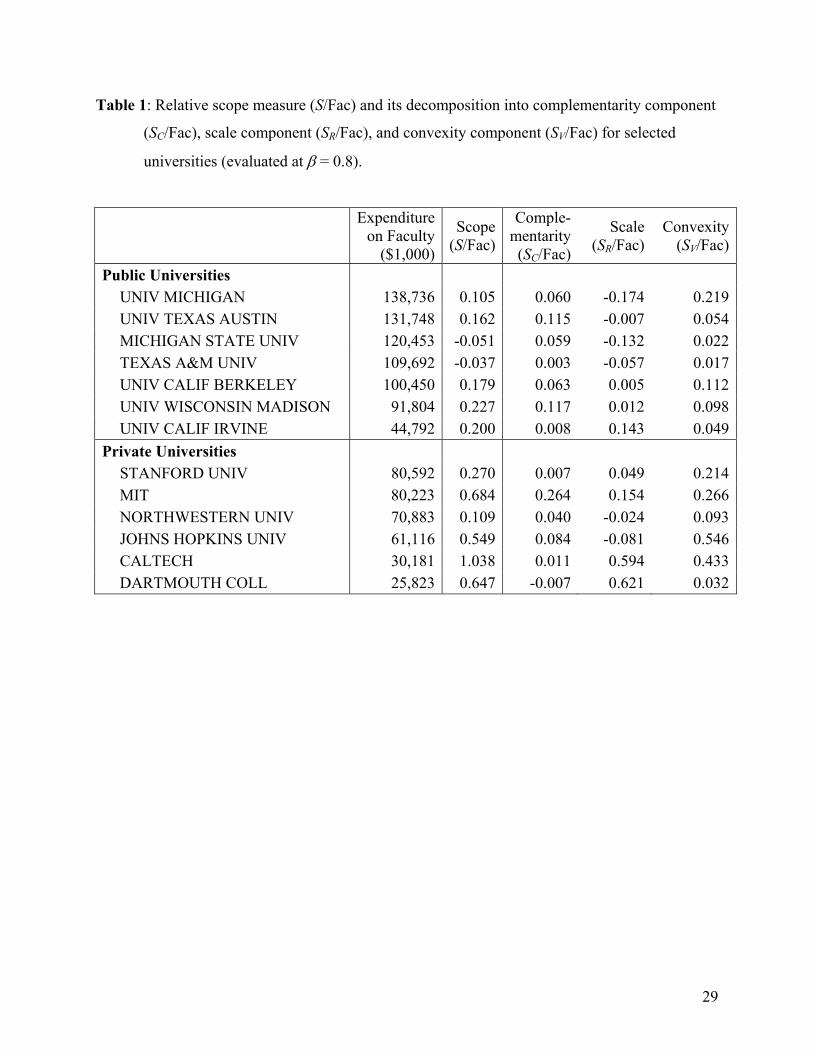
sources of scope. As shown in Table 1, the proportion S/Fac varies from -0.037 (for Texas A&M

University) to 1.038 (for Caltech). As in the larger sample data, the scope estimates in Table 1

reflect the finding that economies of scope are prevalent between patents and more traditional

university outputs. Table 1 also illustrates the finding that the relative measures of S/Fac vary

systematically across universities with these estimates being larger for smaller universities and,

accordingly, for private universities.

21

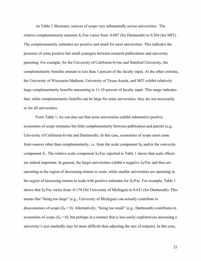
As Table 1 illustrates, sources of scope vary substantially across universities. The

relative complementarity measure SC/Fac varies from -0.007 (for Dartmouth) to 0.264 (for MIT).

The complementarity estimates are positive and small for most universities. This indicates the

presence of some positive but small synergies between research publications and university

patenting. For example, for the University of California-Irvine and Stanford University, the

complementarity benefits amount to less than 1 percent of the faculty input. At the other extreme,

the University of Wisconsin-Madison, University of Texas-Austin, and MIT exhibit relatively

large complementarity benefits amounting to 11-26 percent of faculty input. This range indicates

that, while complementarity benefits can be large for some universities, they are not necessarily

so for all universities.

From Table 1, we can also see that some universities exhibit substantive positive

economies of scope estimates but little complementarity between publication and patents (e.g.,

University of California-Irvine and Dartmouth). In this case, economies of scope must come

from sources other than complementarity, i.e. from the scale component SR and/or the convexity

component SV. The relative scale component SR/Fac reported in Table 1 shows that scale effects

are indeed important. In general, the larger universities exhibit a negative SR/Fac and thus are

operating in the region of decreasing returns to scale, while smaller universities are operating in

the region of increasing returns to scale with positive estimates for SR/Fac. For example, Table 1

shows that SR/Fac varies from -0.174 (for University of Michigan) to 0.621 (for Dartmouth). This

means that “being too large” (e.g., University of Michigan) can actually contribute to

diseconomies of scope (SR < 0). Alternatively, “being too small” (e.g., Dartmouth) contributes to

economies of scope (SR > 0), but perhaps in a manner that is less easily exploited (as increasing a

university’s size markedly may be more difficult than adjusting the mix of outputs). In this case,

22

small universities (e.g., University of California-Irvine, Dartmouth) can exhibit economies of

scope in the absence of complementarity because of scale effects. Additionally, some universities

operating close to the region of constant returns to scale are associated with small SR/Fac (e.g.,

University of California-Berkeley, University of Wisconsin-Madison). Finally, the relative

convexity component SV/Fac reported in Table 1 varies between 0.017 (for Texas A&M) and

0.546 (for Johns Hopkins). As expected, it is non-negative under a convex technology. The

results indicate that the degree of convexity of the technology also varies substantially across

evaluation points.

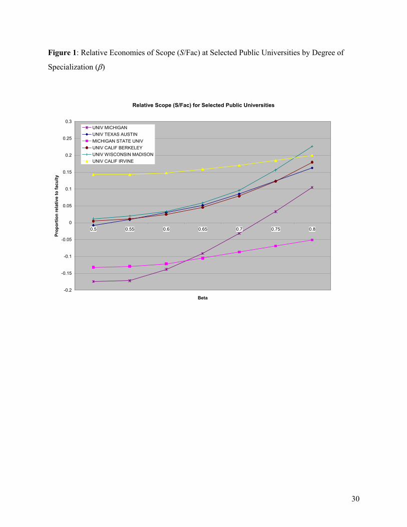
Additional estimates of relative economies of scope are presented in Figures 1 and 2.

Figure 1 depicts for selected public universities how the relative scope measure S/Fac varies with

the degree of specialization, β. In general, scope benefits increase with the degree of

specialization, which demonstrates that the incentives of selected universities to take advantage

of such benefits by combining patenting and article producing activities are most evident under

scenarios associated with high degrees of specialization. However, note that this tendency also

varies across universities. This increase in scope benefits is found to be modest for the University

of California-Irvine, but quite large for the University of Michigan. Figure 2 depicts similar

estimates for selected private universities. Figure 2 illustrates that the relative scope benefits

S/Fac increase with β, strongly so for some universities (e.g., Johns Hopkins) but only mildly so

for others (e.g., Dartmouth). Again, it appears that the benefits of integration across outputs

depend on the degree of specialization.

Additional information on complementarity effects is presented in Figures 3 and 4 for

public and private universities, respectively. These figures depict how the relative

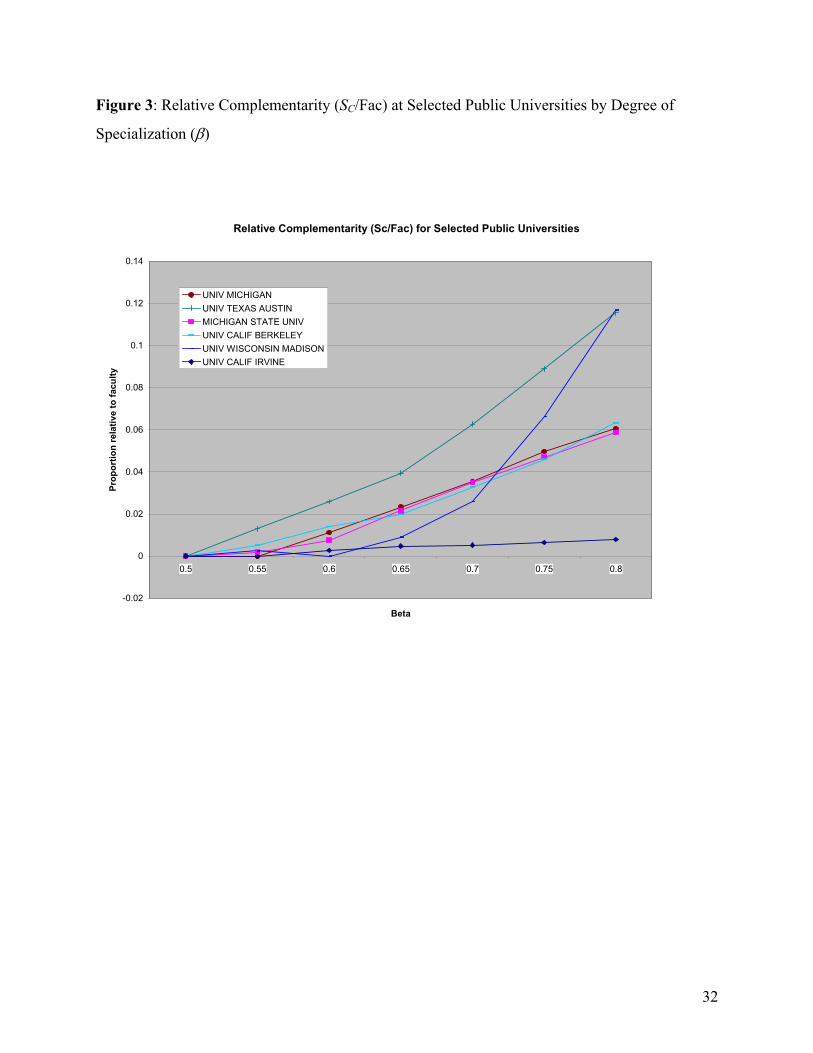
complementarity component SC/Fac varies with the degree of specialization β ∈ [0.5, 0.8]. Since

23

SC = 0 when β = 0.5, we find in general that SC/Fac tends to increase with β. Again, this indicates

that complementarity effects tend to be larger when comparing a university as an integrated firm

with two more highly specialized firms. This is true for public universities as well as private

universities. However, the patterns differ between public and private universities. For the

former, except for the University of California-Irvine (for which changing β has little impact),

SC/Fac tends to increase significantly as β rises, reflecting the strong potential for exploiting the

apparent complementarity between publications and patents by producing them in an integrated

fashion. As shown in Figure 3, the rate of increase is particularly high for the University of

Wisconsin-Madison for β ≥ 0.7, and for the University of Texas-Austin. For these two

universities, the productivity gains due to publication-patent complementarities appear to be

especially large when evaluated at a level above β ≥ 0.7, corresponding to a high degree of

specialization. Figure 4 shows that the relative complementarity effects SC/Fac are small for all

private universities when β ∈ [0.5, 0.65]. Except for Johns Hopkins and MIT, they remain small

for private universities (including here Cal Tech, Stanford, and Northwestern) as the degree of

specialization β rises. Only above β > 0.7 for MIT does there appear to be large scope economies

attributable to complementarity between articles and patents. Overall, these estimates suggest

that the benefits of complementarity vary markedly across universities as well as degree of

specialization, and that complementarities between articles and patents contribute significantly to

scope benefits only for selected universities.

VII. Concluding Remarks

We have presented an economic analysis of scope economies at US universities, with a

focus on the decomposition of economies of scope evaluated directly from the technology. We

24

first developed a conceptual model allowing for the investigation of economies of scope in a

primal framework where the benefits of producing from an integrated firm can be measured

directly from the technology of university production, using Luenberger’s shortage function.

This measure covers both the case of complete specialization (typically found in previous

literature on economies of scope) and the case of partial specialization (suitable for investigating

economies of scope in university production). Further, this approach allows for a decomposition

of economies of scope into three additive parts measuring scale effects, complementarity effects

and convexity effects. Relying on a non-parametric approach, we first recovered the production

technology of 92 US universities using 1995-1998 data, and evaluated the associated

Luenberger’s shortage function. Then, measures of economies of scope and their decomposition

results are obtained and analyzed.

Our analysis uncovered several important findings. First, we find that economies of scope

are prevalent between patents and more traditional university outputs. Second, we documented

how economies of scope measures of US universities during the 1995 to 1998 period vary with

university size. We find that economies of scale (diseconomies of scale) associated with small

(large) universities contribute to generating economies (diseconomies) of scope. Third, we

uncovered evidence that complementarity effects are size-sensitive and vary across universities.

We found large complementarity benefits between research articles and patents for a few

universities, both private (MIT) and public (University of Texas-Austin, University of

Wisconsin-Madison). However, such complementarity effects are found to be negligible for

small universities, as well as many large universities. This suggests that synergies between

articles and patents exist but are not widespread within the academic community. Fourth, our

decomposition of scope effects into scale component, complementarity component and

25

convexity component provides useful information on the sources of scope benefits. For example,

we found that scope effects tend to be important for small universities because of scale effects

(and not because of complementarity effects). However, for the large public/private universities,

scale effects tend to be smaller, while complementarity effects can become more important.

Our analysis suggests a need for future research to evaluate whether economies of scope

may have changed over time. Also, our finding that economies of scope and complementarities

can vary a lot across universities raises the question: what factors contribute to the presence of

scope economies and complementarities in the research activities at U.S. universities? That

undertaking appears challenging, because at the core of the university research mission is the

creative process of inquiry, discovery, invention, and innovation. For example, given the

complexities involved in the dynamic production of new knowledge, identifying why major

complementarities in research activities arise for some universities (e.g., MIT or the University

of Wisconsin-Madison) and not others may be quite difficult. Nonetheless, exploring such issues

has considerable value, even if it could only identify that some complementarity and scope

benefits may not be easily transferable across universities. Finally, while this paper focused on

the presence and sources of scope economies at U.S. research universities, it would be useful to

undertake similar analyses of other multiproduct industries (e.g., the banking industry, R&D in

life sciences, the food industry, and environmental management).

26

References

Adams, Amy, “Citation Analysis: Harvard Tops in Scientific Impact.” Science. 1998, 281

(September 25), 1936.

Afriat, Sidney, “Efficiency Estimation of Production Functions” International Economic Review ,

1972, 13, 568-598.

Azoulay, Pierre, Ding, Waverly, and Stuart, Toby, “The Impact of Academic Patenting on Public

Research Output.” Working Paper, Columbia University, New York, July 2004.

Baumol, William J., Panzar, John C., and Willig, Robert D, Contestable Markets and the Theory

of Industry Structure. Harcourt Brace Jovanovich, Inc., New York, 1982.

Branstetter, Lee, “Is Academic Science Driving a Surge in Industrial Innovation? Evidence from

Patent Citations.” Working Paper, Columbia Business School, New York, January 2003.

Chambers, Robert G., Chung, Yangho and Färe, Rolf, “Benefit and Distance Functions” Journal

of Economic Theory, 1996, 76, 407-419.

Cohn, Elchanan, Rhine, Sherrie L.W. and Santos, Maria C., “Institutions of Higher Education as

Multi-product Firms: Economies of Scale and Scope” Review of Economics and

Statistics,1989, 71, 284-290.

De Groot, Hans, MacMahon, Walter W. and Volkwein, J. Fredericks, “The Cost Structure of

American Research Universities” Review of Economics and Statistics, 1991, 73, 424-431.

Färe, Rolf, and Grosskopf, Shawna, “Theory and Applications of Directional Distance

Functions” Journal of Productivity Analysis, 2000, 13, 93-103.

27

Foltz, Jeremy D., Barham, Bradford L. Chavas, Jean Paul and Kim, Kwansoo, “Efficiency and

Technological Change at US Research Universities” Working Paper, University of

Wisconsin, Madison, 2005.

Hall, Bronwyn H., Jaffe, Adam B. and Trajtenberg, Manuel, “The NBER Patent Citation Data

File: Lessons, Insights, and Methodological Tools.” in A. Jaffe and M. Trajtenberg eds.

Patents, Citations, and Innovations: A Window on the Knowledge Economy. Cambridge

MA: MIT University Press. 2003a.

Hall, Bronwyn H., Link, Albert N. and Scott, John, T., “Universities as Research Partners”

Review of Economics and Statistics, 2003b, 85, 485-491.

Henderson, Rebecca, Jaffe, Adam, B. and Trajtenberg, Manuel, “University as a Source of

Commercial Technology: A Detailed Analysis of University Patenting, 1965-1998.”

Review of Economics and Statistics, 1998, 80, 119-27.

ISI Web of Science, “Science Citation Index (SCI)”. Thompson Scientific Publishing. Accessed

online at http://isi0.isiknowledge.com/ (Last accessed May, 2004).

Jaffe, Adam, B., “Real Effects of Academic Research” American Economic Review, 1989, 79,

957-970.

Jensen, Richard, A., and Thursby, Marie C., “Proofs and Prototypes for Sale: The Licensing of

University Inventions” American Economic Review, 2001, 91, 240-259.

Luenberger, David G., Microeconomic Theory. McGraw-Hill, Inc., New York, 1995.

Milgrom, Paul, and Roberts, John, “The Economics of Modern Manufacturing: Technology,

Strategy and Organization” American Economic Review, 1990, 80, 511-528.

28

National Science Foundation, "NSF Webcaspar: Your Virtual Bookshelf of Statistics on

Academic Science and Engineering." http://caspar.nsf.gov/ (Last accessed July, 2004).

Sampat, Bhaven N., Mowery, David C.,and Ziedonis Arvids A., “Changes in University Patent

Quality after the Bayh-Dole Act: A Re-Examination.” Working Paper, Georgia Institute

of Technology, 2003.

Sav, G. Thomas, “Higher Education Costs and Scale and Scope Economies” Applied Economics,

2004, 36, 607-614.

Shephard, Ronald, Theory of Cost and Production Functions, Princeton University Press.

Princeton, NJ, 1970.

Scotchmer, Suzanne, Innovation and Incentives. MIT Press, Cambridge, MA, 2004.

U. S. Patent Office, "Patent Bibliographic and Abstract Database."

http://www.uspto.gov/patft/index.html. (Last accessed July, 2004).

Varian, Hal R., “The Nonparameteric Approach to Production Analysis” Econometrica, 1984, 52,

579-597.

29

Table 1: Relative scope measure (S/Fac) and its decomposition into complementarity component

(SC/Fac), scale component (SR/Fac), and convexity component (SV/Fac) for selected

universities (evaluated at β = 0.8).

Expenditure

on Faculty ($1,000)

Scope(S/Fac)

Comple-mentarity (SC/Fac)

Scale (SR/Fac)

Convexity (SV/Fac)

Public Universities UNIV MICHIGAN 138,736 0.105 0.060 -0.174 0.219UNIV TEXAS AUSTIN 131,748 0.162 0.115 -0.007 0.054MICHIGAN STATE UNIV 120,453 -0.051 0.059 -0.132 0.022TEXAS A&M UNIV 109,692 -0.037 0.003 -0.057 0.017UNIV CALIF BERKELEY 100,450 0.179 0.063 0.005 0.112UNIV WISCONSIN MADISON 91,804 0.227 0.117 0.012 0.098UNIV CALIF IRVINE 44,792 0.200 0.008 0.143 0.049

Private Universities STANFORD UNIV 80,592 0.270 0.007 0.049 0.214MIT 80,223 0.684 0.264 0.154 0.266NORTHWESTERN UNIV 70,883 0.109 0.040 -0.024 0.093JOHNS HOPKINS UNIV 61,116 0.549 0.084 -0.081 0.546CALTECH 30,181 1.038 0.011 0.594 0.433DARTMOUTH COLL 25,823 0.647 -0.007 0.621 0.032

30

Figure 1: Relative Economies of Scope (S/Fac) at Selected Public Universities by Degree of

Specialization (β)

Relative Scope (S/Fac) for Selected Public Universities

-0.2

-0.15

-0.1

-0.05

0

0.05

0.1

0.15

0.2

0.25

0.3

0.5 0.55 0.6 0.65 0.7 0.75 0.8

Beta

Prop

ortio

n re

lativ

e to

facu

lty

UNIV MICHIGANUNIV TEXAS AUSTINMICHIGAN STATE UNIVUNIV CALIF BERKELEYUNIV WISCONSIN MADISONUNIV CALIF IRVINE

31

Figure 2: Relative Economies of Scope (S/Fac) at Selected Private Universities by Degree of

Specialization (β)

Relative Scope (S/Fac) for Selected Private Universities

-0.2

0

0.2

0.4

0.6

0.8

1

1.2

0.5 0.55 0.6 0.65 0.7 0.75 0.8

Beta

Prop

ortio

n re

lativ

e to

facu

lty

STANFORD UNIVMITNORTHWESTERN UNIVJOHNS HOPKINS UNIVCALTECHDARTMOUTH COLL

32

Figure 3: Relative Complementarity (SC/Fac) at Selected Public Universities by Degree of

Specialization (β)

Relative Complementarity (Sc/Fac) for Selected Public Universities

-0.02

0

0.02

0.04

0.06

0.08

0.1

0.12

0.14

0.5 0.55 0.6 0.65 0.7 0.75 0.8

Beta

Prop

ortio

n re

lativ

e to

facu

lty

UNIV MICHIGANUNIV TEXAS AUSTINMICHIGAN STATE UNIVUNIV CALIF BERKELEYUNIV WISCONSIN MADISONUNIV CALIF IRVINE

33

Figure 4: Relative Complementarity (SC/Fac) for Selected Private Universities by Degree of

Specialization (β)

Relative Complementarity (Sc/Fac) for Selected Private Universities

-0.05

0

0.05

0.1

0.15

0.2

0.25

0.3

0.5 0.55 0.6 0.65 0.7 0.75 0.8

Beta

Prop

ortio

n re

lativ

e to

facu

lty

STANFORD UNIVMITNORTHWESTERN UNIVJOHNS HOPKINS UNIVCALTECHDARTMOUTH COLL

34

Appendix A

Proof of Proposition 1: From equation (4), economies of scope are defined as

S ≡ σ(-½ x, β yA1, (1-β) yA2, ½ yB, g) + σ(-½ x, (1-β) yA1, β yA2, ½ yB, g)

- σ(x, y, g) > 0.

When σ(z, g) is continuous in z and differentiable almost everywhere in y, this can be

alternatively written as

S = - ∫ −

A2

A2

y β

y β)(1[∂σ/∂γ(-½ x, β yA1, γ, ½ yB, g) - ∂σ/∂γ(-½ x, (1-β) yA1, γ, ½ yB, g)] dγ

+ σ(-½ x, β yA, ½ yB, g) + σ(-½ x,(1-β) yA, ½ yB, g) - 2 σ(½ z, g),

+ 2 σ(½ z, g) - σ(-x, y, g).

Lemma 1: σ(k z, g)

>=<

k σ(z, g) under

IRTSCRTSDRTS

.

Proof: By definition, the technology exhibits increasing return to scale (IRTS), constant return to

scale (CRTS), or decreasing return to scale (DRTS) when, for all α > 1, α F ⊂ F, α F = F,

or α F ⊃ F, respectively. Let k ∈ (0, 1). Consider the case where there is a γ satisfying (k

z - γ g) ∈ F. Then

σ(k z, g) = minγ {γ: (k z - γ g) ∈ F},

= k minδ {δ: (z - δ g) ∈ (1/k) F}, where δ = γ/k,

>=<

k σ(z, g) when (1/k) F

⊂=⊃

F, i.e., under

IRTSCRTSDRTS

.

35

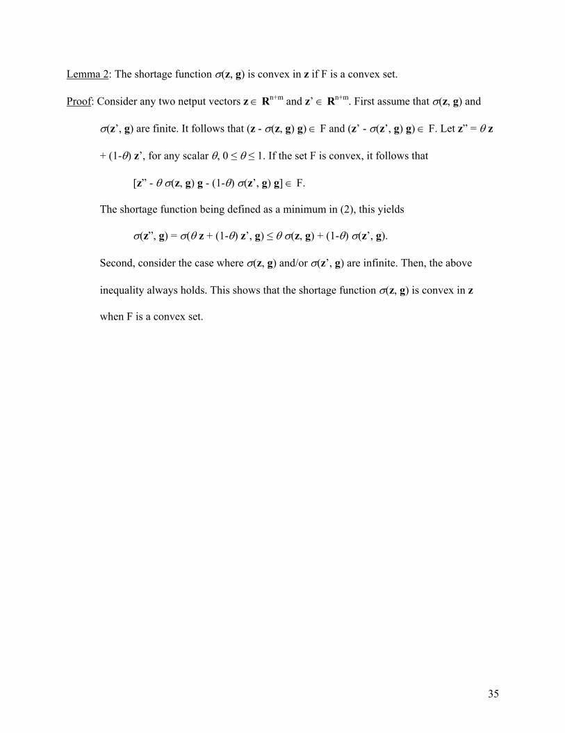
Lemma 2: The shortage function σ(z, g) is convex in z if F is a convex set.

Proof: Consider any two netput vectors z ∈ Rn+m and z’ ∈ Rn+m. First assume that σ(z, g) and

σ(z’, g) are finite. It follows that (z - σ(z, g) g) ∈ F and (z’ - σ(z’, g) g) ∈ F. Let z” = θ z

+ (1-θ) z’, for any scalar θ, 0 ≤ θ ≤ 1. If the set F is convex, it follows that

[z” - θ σ(z, g) g - (1-θ) σ(z’, g) g] ∈ F.

The shortage function being defined as a minimum in (2), this yields

σ(z”, g) = σ(θ z + (1-θ) z’, g) ≤ θ σ(z, g) + (1-θ) σ(z’, g).

Second, consider the case where σ(z, g) and/or σ(z’, g) are infinite. Then, the above

inequality always holds. This shows that the shortage function σ(z, g) is convex in z

when F is a convex set.

36

Appendix B: Data

Patents

Patent data were culled from the NBER patent database, where they were identified as

having a university assignee. Patents assigned to the University of California system were

associated with a campus (Berkeley, Davis, Los Angeles, etc.) by the location of their authors

through searches of campus directories. Relative citations for patents were generated by year

and by patent class comparing each individual patent to the universe of all patents in that class

(whether owned by universities or not). A university’s patent count for that year is then adjusted

by the ratio of number of citations received to the expected citations for that portfolio:

)(

##citationsE

receivedcitationspatentsPatentsAdjustedQuality ×=

where the number of expected citations, E(citations) is calculated as the number of citations that

same portfolio of patents would receive if each patent received the average citation rate for its

US patent class for that year.

Articles

Article data were culled from the ISI-Web of Science database based on universities

included in their “University Science Indicators” and categories established in that same

document. The Web of Science includes only the major journals in a field as identified by

impact factors, such that our article measures necessarily cut out articles written for lesser

journals. In addition the citation measures are only for citations in other major journals. This

truncation, we believe serves our purposes of adding a subtle quality measure even to our

quantity measures. Articles listed in all science disciplines were chosen.

Relative citations for articles were generated by category compared to citations of other

articles assigned to the universities in the sample, rather than to all articles, and these measures

were constructed annually. The same techniques of generating relative citations used for patents

were used for articles.

Universities included in the sample:

Arizona State U., Boston U., Brandeis U., Brown U., Caltech, Carnegie Mellon U., Case

Western Reserve U., Colorado State U., Cornell U., Dartmouth College, Emory U., Florida State

37

U., Georgetown U., Georgia Inst. of Technology., Harvard U., Indiana U., Iowa State U., Johns

Hopkins U., Lehigh U., Loyola U., Michigan State U., MIT, N Carolina State U., New Mexico

State U., Northwestern U., Ohio State U., Oregon State U., Penn State U., Princeton U., Purdue

U., Rice U., Stanford U., Syracuse U., Texas A&M U., Tufts U., U. Alabama, U. Alaska, U.

Arizona, U. C. Berkeley, U. C. Davis, U. C. Irvine, U. C. Los Angeles, U. C. Riverside, U. C.

San Diego, U. C. Santa Barbara, U. C. Santa Cruz, U. Chicago, U. Cincinnati, U. Colorado, U.

Connecticut, U. Delaware, U. Florida, U. Georgia, U. Hawaii, U. of Illinois Chicago, U. Illinois

Urbana, U. Iowa, U. Kansas, U. Kentucky, U. Maryland Baltimore, U. Maryland College

Park, U. Miami, U. Michigan, U. Minnesota, U. Missouri, U. N. Carolina Chapel Hill, U.

Nebraska, U. New Hampshire, U. New Mexico, U. Oregon, U. Penn, U. Pittsburgh, U.

Rochester, U. So Calif, U. Tennessee, U. Texas Austin, U. Texas Houston, U. Utah, U.

Vermont, U. Virginia, U. Washington, U. Wisconsin Madison, Utah State U., Vanderbilt

U., Virginia Polytech Inst, W. Virginia U., Wake Forest U., Washington State U., Washington

U., Wayne State U., Yale U., Yeshiva U.

38

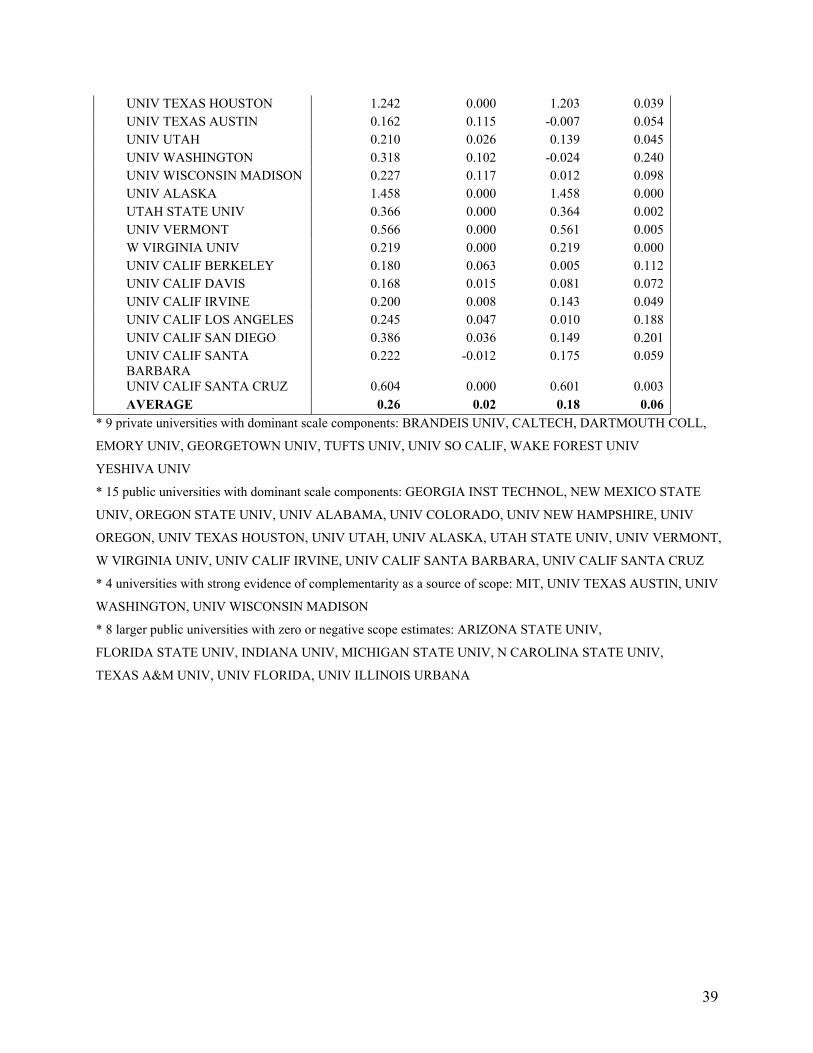
Table B-1: Relative scope measure (S/Fac) and its decomposition into complementarity

component (SC/Fac), scale component (SR/Fac), and convexity component (SV/Fac) for 52

universities (evaluated at β = 0.8).

Scope

(S/Fac)

Comple-mentarity(SC/Fac)

Scale (SR/Fac)

Convexity (SV/Fac)

Private Universities BOSTON UNIV 0.186 0.007 0.098 0.081 BRANDEIS UNIV 1.021 0.000 1.021 0.000 CALTECH 1.038 0.011 0.594 0.433 DARTMOUTH COLL 0.647 -0.007 0.621 0.032 EMORY UNIV 0.362 -0.003 0.285 0.080 GEORGETOWN UNIV 0.245 -0.012 0.204 0.054 HARVARD UNIV 1.314 0.017 0.022 1.275 JOHNS HOPKINS UNIV 0.548 0.084 -0.081 0.546 MIT 0.684 0.264 0.154 0.266 NORTHWESTERN UNIV 0.109 0.040 -0.024 0.093 STANFORD UNIV 0.270 0.007 0.049 0.214 TUFTS UNIV 0.271 0.001 0.214 0.056 UNIV PITTSBURGH 0.076 0.023 -0.104 0.156 UNIV SO CALIF 0.147 0.001 0.127 0.019 WAKE FOREST UNIV 0.824 -0.003 0.816 0.011 YESHIVA UNIV 1.273 -0.003 1.260 0.016 AVERAGE 0.56 0.03 0.33 0.21

Public Universities ARIZONA STATE UNIV -0.003 0.006 -0.011 0.002 FLORIDA STATE UNIV 0.009 0.008 -0.007 0.007 GEORGIA INST TECHNOL 0.333 -0.005 0.307 0.031 INDIANA UNIV 0.019 0.000 -0.007 0.026 MICHIGAN STATE UNIV -0.051 0.059 -0.132 0.022 NEW MEXICO STATE UNIV 0.343 0.000 0.339 0.003 N CAROLINA STATE UNIV 0.068 0.023 0.006 0.039 OHIO STATE UNIV -0.080 0.027 -0.162 0.054 OREGON STATE UNIV 0.477 -0.013 0.461 0.029 PENN STATE UNIV 0.094 0.051 -0.035 0.078 TEXAS A&M UNIV -0.037 0.003 -0.057 0.017 UNIV ALABAMA 0.173 0.020 0.114 0.039 UNIV COLORADO 0.134 -0.001 0.103 0.032 UNIV FLORIDA 0.011 0.041 -0.095 0.065 UNIV ILLINOIS URBANA -0.040 0.032 -0.177 0.104 UNIV MICHIGAN 0.105 0.060 -0.174 0.219 UNIV MINNESOTA 0.112 0.026 -0.104 0.191 UNIV NEW HAMPSHIRE 0.459 0.000 0.459 0.000 UNIV OREGON 0.381 0.000 0.380 0.001 UNIV TENNESSEE 0.092 0.011 0.014 0.067

39

UNIV TEXAS HOUSTON 1.242 0.000 1.203 0.039 UNIV TEXAS AUSTIN 0.162 0.115 -0.007 0.054 UNIV UTAH 0.210 0.026 0.139 0.045 UNIV WASHINGTON 0.318 0.102 -0.024 0.240 UNIV WISCONSIN MADISON 0.227 0.117 0.012 0.098 UNIV ALASKA 1.458 0.000 1.458 0.000 UTAH STATE UNIV 0.366 0.000 0.364 0.002 UNIV VERMONT 0.566 0.000 0.561 0.005 W VIRGINIA UNIV 0.219 0.000 0.219 0.000 UNIV CALIF BERKELEY 0.180 0.063 0.005 0.112 UNIV CALIF DAVIS 0.168 0.015 0.081 0.072 UNIV CALIF IRVINE 0.200 0.008 0.143 0.049 UNIV CALIF LOS ANGELES 0.245 0.047 0.010 0.188 UNIV CALIF SAN DIEGO 0.386 0.036 0.149 0.201 UNIV CALIF SANTA

BARBARA 0.222 -0.012 0.175 0.059

UNIV CALIF SANTA CRUZ 0.604 0.000 0.601 0.003 AVERAGE 0.26 0.02 0.18 0.06

* 9 private universities with dominant scale components: BRANDEIS UNIV, CALTECH, DARTMOUTH COLL,

EMORY UNIV, GEORGETOWN UNIV, TUFTS UNIV, UNIV SO CALIF, WAKE FOREST UNIV

YESHIVA UNIV

* 15 public universities with dominant scale components: GEORGIA INST TECHNOL, NEW MEXICO STATE

UNIV, OREGON STATE UNIV, UNIV ALABAMA, UNIV COLORADO, UNIV NEW HAMPSHIRE, UNIV

OREGON, UNIV TEXAS HOUSTON, UNIV UTAH, UNIV ALASKA, UTAH STATE UNIV, UNIV VERMONT,

W VIRGINIA UNIV, UNIV CALIF IRVINE, UNIV CALIF SANTA BARBARA, UNIV CALIF SANTA CRUZ

* 4 universities with strong evidence of complementarity as a source of scope: MIT, UNIV TEXAS AUSTIN, UNIV

WASHINGTON, UNIV WISCONSIN MADISON

* 8 larger public universities with zero or negative scope estimates: ARIZONA STATE UNIV,

FLORIDA STATE UNIV, INDIANA UNIV, MICHIGAN STATE UNIV, N CAROLINA STATE UNIV,

TEXAS A&M UNIV, UNIV FLORIDA, UNIV ILLINOIS URBANA

40

Footnotes

１ Note that other measures have been developed in the literature. They include the directional

distance function Dg(z, g) discussed by Robert G. Chambers, Yangho Chung, and Rolf Färe and

Rolf Färe, and Shawna Grosskopf: Dg(z, g) ≡ maxβ {β: (z + β g) ∈ F}. Since it satisfies σ(z, g) =

-Dg(z, g), it should be clear that the analysis presented below could be presented equivalently

using the directional distance function. Other measures include Shephard’s output distance

function DO(z) ≡ minθ {θ: (-x, y/θ) ∈ F}, and Shephard’s input distance function DI(z) ≡ maxθ

{θ: (-x/θ, y) ∈ F}. The relationships between these functions and the shortage function have

been analyzed in the literature (Rolf Färe, and Shawna Grosskopf; Robert G. Chambers, Yangho

Chung, and Rolf Färe). However, by measuring input or output proportions, the Shephard’s

functions are not additive across firms. As such they do not provide attractive measurements for

analyzing economies of scope.

２ Note that, in the case where IB = ∅ and β = 1, this involves no loss of generality since any

partition of IA can always be decomposed into a series of binary partitions.

３ Below, the linear programming problem (6) is solved using GAMS software.