research regarding the use of new systems to control … regarding the use of new systems to control...

Research regarding the use of new systems to control fluid flow in pipelines

OLIMPIU STOICUTA, MARIN SILVIU NAN, GABRIEL DIMIRACHE, NICOLAE BUDA,

DAN LIVIU DANDEA Control, Applied Informatics and Computers Department; Department of Machines, Installations and

Transport University of Petrosani

20 University Street, Petroşani ROMANIA

[email protected], [email protected], [email protected], [email protected], [email protected]

http://www.ime.upet.ro/mi/index.html Abstract: - In this paper a research is made on the design of a new fluid flow control system on transport pipelines. The flow control system is based on a sensorless speed control system of an induction motor with the squirrel – cage. The estimator component for rotor flux and speed from the induction motor speed control system is an Extended Gopinath Observer. Key-Words: - Extended Gopinath Observer, Sensorless Control, Flow Control Simulation, Centrifugal Pumps. 1 Introduction This paper presents a new flux and rotor speed observer [9] called an Extended Gopinath Observer (EGO). The design of the EGO observer is done based on an adaptive mechanism using the notion of Popov hyperstability [7]. Thus, this type of observer is included in the estimation methods based on an adaptation mechanism, along with the Extended Luenberger Observer (ELO) proposed by Kubota [4] and the Model Adaptive System (MRAS) observer proposed by Schauder [1].

This type of speed control system is used in the second part of the paper in the design of a pipe flow control system.

2 The Extended Gopinath Observer The equations that define the rotor flux Gopinath observer are [9]:

* * * *

s s s sa b 12 11r

* *s s s21 22r r

d ˆi a i a i a b udtd d dˆ ˆa i a g i idt dt dt

(1)

where:

* * *11 a ba a a ; * * *

r12 13 14 pa a j a z ; * *21 31a a

** m13 * * * *

s r r

LaL L T

;*

* m14 * * *

s r

LaL L

;*

* m31 *

r

LaT

* *r22 33 pa a j z ; *

33 *r

1aT

; *11 * *

s

1bL

;

** ss *

s

LTR

*

* rr *

r

LTR

;

2*m*

* *s r

L1

L L

; *

a * *s

1aT

;*

*b * *

r

1aT

.

In the relations above, are marked with “*” the identified electrical sizes of the induction motor.

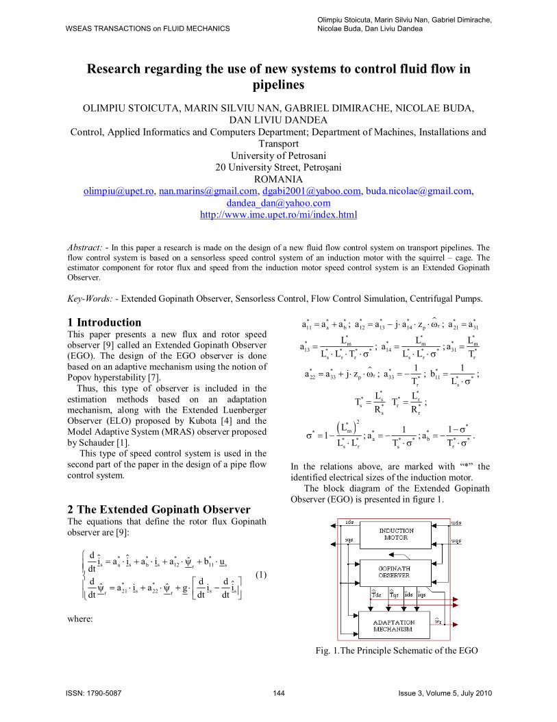
The block diagram of the Extended Gopinath Observer (EGO) is presented in figure 1.

Fig. 1.The Principle Schematic of the EGO

WSEAS TRANSACTIONS on FLUID MECHANICSOlimpiu Stoicuta, Marin Silviu Nan, Gabriel Dimirache, Nicolae Buda, Dan Liviu Dandea

ISSN: 1790-5087 144 Issue 3, Volume 5, July 2010

The essential element in the stability of the

Gopinath flux observer is the g gain, which is a complex number in the following form:

a bg g j g (2)

In order to design this type of estimator we need to position the estimator’s poles in the left Nyquist plane so that the estimator’s stability is assured.

The expressions ga and gb after the pole positioning are [9]:

* *31 33

a 2 2*33 p r

*31 p r

b 2 2*33 p r

a aga z

a zg

a z

(3)

In these conditions the Gopinath rotor flux

observer is completely determined. Next, in order to determine the adaptation

mechanism used to estimate the rotor speed, we will consider as a reference model the „stator curents - rotor fluxes” model of the induction engine and as an ajustable model, the model of the Gopinath rotor flux observer. The equations mentioned above written under the input-state-output canonic form are: Reference model:

d x A x B udt

dy C xdt

(4)

Ajustable model:

1

d ˆ ˆ ˆx A x A x B u G y ydt

dˆ ˆy C xdt

(5)

where:

11 12

21 22

a aA

a a

; * *a 12

*22

a aA

0 a

; *b

1 *21

a 0A

a 0

0G

g

; s

r

ix

; s

r

ix

;

su u ; 11bB

0

; C 1 0 .

In the above relations we marked with „~” the Gopinath estimator’s matrices which are dependent upon the rotor speed, which in turn needs to be estimated based on the adaptation mechanism.

Next, in order to determine the expression that defines the adaptation mechanism we will assume that the identified electric sizes are identical with the real electric sizes of the induction engine.

In other words:

*ij ija a ;i, j 1, 2 and *

11 11b b .

In order to build the adaptive mechanism, for start we will calculate the estimation error given by the difference:

ˆe x xx (6) Derivation the relation (6) in relation with time

and by using the relations (4) and (5) the relation (6) becomes:

1

d de A A x A x G C ex xdt dt (7)

If the determinant, 2det I G C 0 , then it

exists a unique inverse matrix 1

2M I G C

so that the expression (7) can be written like this:

1 1d e M A A e M A A A xx xdt

(8)

Equation (8) describes a linear system defined by

the term 1M A A ex in inverse connection

with a non linear system defined by the term ye

which receives at input the error y xe C e between the models and has at the output the term:

1M A A A x (9)

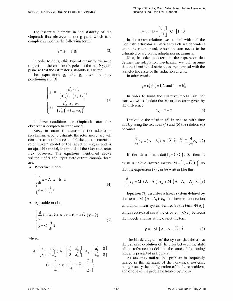
The block diagram of the system that describes

the dynamic evolution of the error between the state of the reference model and the state of the tuning model is presented in figure 2.

As one may notice, this problem is frequently treated in the literature of the non-linear systems, being exactly the configuration of the Lure problem, and of one of the problems treated by Popov.



Fig. 2: The block diagram of the system that describes the dynamic evolution of the error

between the state of the reference model and the state of the control model

Considering, according to the Popov terminology, the non-linear block described by

ey the integral input- output index associated to

it is:

1t T0 1 y0

t , t Re e t t dt (10)

In order for block to be hyper-stable a necessary

condition is:

1t T 21 y0

0, t Re e t t dt 0 (11)

for any input-output combination and where 0 is a positive constant.

In the above relation we marked with Tye the

following expression

Tyye e 0 (12)

Obtained in order to keep the compatibility

between the input and output dimensions, and ye represents the conjugate of the complex variable ye .

Under these circumstances, using the relation (9) the expression (11) becomes:

1t T 21 y 10

0, t Re e t M A A A xdt 0

(13) Next we assume that the error 1M A A A

is determined only by the rotor speed of the induction machine. In this case we may write:

r1 r erM A A A A (14)

where: 14 p

erp 14

0 j a zA

0 j z 1 a g

.

For any positive derivable f function we can

demonstrate the following inequality:

1t 211 0

KdfK f dt f 0dt 2

(15)

On the other hand, using the relation (14), the

expression (13) becomes:

1t T 2r1 y er r0

0,t Re e t A x dt 0

(16)

By combining the relations (15) and (16) we can write the following relations:

rr

Ty er 1

fdfˆRe e A x Kdt

(17)

Because 1K is a constant and then, in case of a

slower r parameter variation related to the adaptive law, we can write:

T

r i y er ˆk Re e A x dt (18) After replacing the variables that define the

above expression (18) and taking into account the arbitrary nature of the iK positive constant we obtain:

r qr dri yd yqk e e dt (19)

where dsyd dse i i and qsyq qse i i . Sometimes, instead of the adaptation law (19) we

can use the following form: r qr dr qr drR yd yq i yd yqK e e k e e dt

(20) From the above relation we ca observe that a

new proportional component apears from the desire to have 2 coefficients that can control the speed estimation dynamics. This fact isn’t always necesary



because we can obtain very good results by using only expresion (19).

Thus expresion (20) represents the general formula of the adaptation mechanism where RK represents the proportionality constant and

i R RK K T ; where RT represents the integration time of the proportional-integral regulator that defines the adaptation mechanism.

3 The Mathematical Description of the Vector Control System

The block diagram of the control system of the mechanical angular speed r of the induction engine with a discreet orientation after the rotor flux (DFOC) is presented in figure 3.

In figure 3 were marked with B1 the control block of the speed control system with direct orientation after the rotor flux (DFCO) and with B2 the extended Gopinath estimator block (EGO).

Some of the equations that define the vector control system are given by the elements which compose the field orientation block and consist of:

Fig.3 The block diagram of the DFOC vector control system which contains an EGO loop. [9]

stator tensions decoupling block (C1Us):

rrds dsr r

r rrr r

2qs

qsr11 13 r 31 p11 r

ds qsdsr rqs 11 qs 14 p r 31 p

11 r

1 iu b v a a z ib

1 i iu b v a z a z i

b

(21) PI flux controller (PI_ψ) defined by the K proportionality constant and the T integration time:

r

6r r

ds 6 r r

dxdt

Ki x K

T

(22)

couple PI controller (PI_Me) defined by the MK proportionality constant and the MT integration time:

r

7e e

Mqs 7 M e e

M

dx M Mdt

Ki x K M MT

(23)

Flux analyzer (AF):



2 2

dr qrr

qr drr r

r r

sin ; cos

(24)

current PI controller (PI_I) defined by the iK proportionality constant and the iT integration time:

rr

rr r

9dsds

idsds 9 i ds

i

dx i idt

Kv x K i iT

(25)

rr

rr r

10qsqs

iqsqs 10 i qs

i

dx i idt

Kv x K i iT

(26)

the calculate of the couple block (C1Me):

rqse a rM K i (27)

where: ma p

r

L3K z2 L

; pz is the pole pairs number.

In these conditions the vector control system is completely defined.

4 Pipe flow control system design The flow control system based on the modification of the speed of the centrifugal pump is presented in figure number 4.

Fig. 4 Conventional representation o a flow control

The following notations were used in figure 3: TD - flow transducer SPC -centrifugal pump L - the length of the pipe, from the pump to the flow transducer D - the interior diameter of the pipe P - the pressure drop on the length L of the pipe

F - inlet flow of the oil F* - prescribed flow for the control system PI FLOW - integral proportional type flow regulator DFOC SPEED - speed control system presented in figure 2.

One of the main problems in the practical implementation of a speed control system for an induction motor is the controller tuning.

In present, the controllers tuning of the induction motors speed control systems is made only through experimental methods, and the time allocated for this type of tests is a really long one.

The paper deals with the analytical tuning controllers through the method of repartition of zeros - poles and the symmetry criteria and module Kessler instance. [9]

Therefore, for the regulators composing block B2 of the speed control system the following analytical adjustment formulas are used. Current controller:

i *11

1Ta

; i * *11 d1

1Kb T

(28)

Flux controller:

*rT T ;

*r

* *m d1

TK2 L T

(29)

Couple controller:

*M d1T T ;

*Td1KM * *K Ta r d2

(30)

Speed controller:

24

*4 d2

T 1K

2 K T

;

* 2d2

3

T 1T 4

1

;

*d 2

4

TT

(31)

where: 41KF

and 4JTF

.

In the above mentioned formulas, *1dT and *

2dT are two time constancies imposed considering they need to respect the following conditions:

* *d1 rT T ; *

d2 4T T and * *d 2 d1T T (32)



The proportion and integration coefficients of the PI controller of the adapting mechanism of the Extended Gopinath Observer are determined using the linear equation of the estimation error (8).

The linearization of the relation defining the estimation error is made using an orthogonal benchmark r rd q related to the rotor flux module. Therefore the linear relation of the estimation error is the following:

a bd e M e M udt (33)

where:

a r0 13

3 r0 a

b r0 a r0 33

a aA a 0

g g a

; *4 14 p r

0A a z

0

;

5

a b

0 0 0A 0 0 0

g g 0

; 13 5N I A ; a 3M N A ;

b 4M N A ; rru ; T1 2 3e e e e .

Considering an identical method, the error:

qr dr1 2t e t t e t t (34)

Following the linearization in an orthogonal benchmark r rd q related to the rotor flux, it becomes:

*r 2e (35)

The following equalities have been considered realised when obtaining the previously mentioned linear expressions:

ds0ds0i i ; qs0qs0i i ; *

dr0dr0 r ; qr0qr0 ;

r0r0 (36)

Relation (35) may be written:

eC e (37)

where: *e rC 0 0 .

Therefore, based on relations (33) and (37) after having applied the Laplace Transformer in initial null conditions, the following transfer function is obtained:

1

e e 3 a b

sG s C s I M M

u s

(38)

Relation (38) may also be written:

2

1 0e u 3 2

2 1 0

s h s hG s Ks s s

(39)

where:

2*u p 14 rK z a ; 1 33 a a 13h a a g a ;

0 a 33 13 b r0h a a a g ; 2 a 13 33 ag a a 2 a ; 2 2

1 r0 a 33 a a a 132 a a a a g a ; 2 2

0 r0 a 13 33 a 33 r0 13 b ag a a a a a g a Therefore, the block diagram of the estimated

speed controll system is presented in figure 5.

Fig. 5. Control system used for speed estimation Considering the previously presented facts, the

transfer function of the open system is:

3 2

2 1 0d R u 3 2

2 1 0

s m s m s mG s k Ks s s s

(40)

where: R 1

2R

T h 1mT

; R 0 11

R

T h hmT

; 00

R

hmT

.

Considering the relation (40) the following

expression will be imposed for the determination of the proportionality coefficient of PI regulator composing the adaption mechanism:

Ru d1

1kK T

(41)

where: 2*u p 14 rK z a .

On the other hand, for the selection of the time constant of the controller, the transfer function of the closed system will be presented considering relation (42) defining the transfer function of the open system.

3 2

2 1 00 R u 4 3 2

3 2 1 0

s m s m s mG s k Ks n s n s n s n

(42)



where: 3 2 R un k K ; 2 1 R u 2n k K m ;

1 0 R u 1n k K m ; 0 R u 0n k K m .

It has been observed that for a time constancy: r

RTT2

(43)

considering the transfer function (42), the poles and zeros of the transfer function (42) are found in the left Nyquist plane.

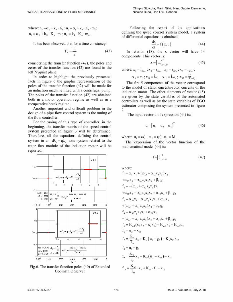
In order to highlight the previously presented facts in figure 6 the graphic representation of the poles of the transfer function (42) will be made for an induction machine fitted with a centrifugal pump. The poles of the transfer function (42) are obtained both in a motor operation regime as well as in a recuperative break regime. Another important and difficult problem in the design of a pipe flow control system is the tuning of the flow controller.

For the tuning of this type of controller, in the beginning, the transfer matrix of the speed control system presented in figure 3 will be determined. Therefore, all the equations defining the control system in an r rd q axis system related to the rotor flux module of the induction motor will be reported.

Fig.6. The transfer function poles (40) of Extended

Gopinath Observer

Following the report of the applications defining the speed control system model, a system of differential equations is obtained:

dx f x,udt

(44)

In relation (18), the x vector will have 14 components. This vector is:

1,14 T

i ix x (45)

where:r1 dsx i ;

r2 qsx i ;r3 drx i ;

r4 qrx i ;

5 rx ; rds11x i ; rqs12x i ; rdr13x .

The firs 5 components of the vector correspond to the model of stator currents-rotor currents of the induction motor. The other elements of vector (45) are given by the state variables of the automated controllers as well as by the state variables of EGO estimator composing the system presented in figure 2. The input vector u of expression (44) is:

T1 2 3u u u u (46) where: *

1 ru ; *2 ru ; 3 ru M .

The expression of the vector function of the mathematical model (44) is:

Ti i 1,14f f

(47)

where:

1 11 1 r 12 p 5 2

13 3 14 p 5 4 11 1

f x ( z x )x

x z x x g

2 r 12 p 5 1

11 2 14 p 5 3 13 4 11 2

f ( z x )x

x z x x x g

3 31 1 32 p 5 2 33 3

r 34 p 5 4 31 1

f x z x x x

( z x )x g

4 32 p 5 1 31 2

r 34 p 5 3 33 4 31 2

f z x x x

( z x )x x g

5 m1 3 2 4 1 m2 5 m3 3f K (x x x x ) K x K u

6 2 13f u x

7 8 1 3 a 13 12Kf x K u g K x xT

8 1 3f u g

9 6 2 13 11

Kf x K u x x

T

M10 7 M 7 12

M

Kf x K f xT



* * * *11 a 11 r 12 b 1 13 13 11 1f a x x a x a x b g

* * * *12 r 11 a 12 b 2 14 p 3 13 11 2f x a x a x a z g x b g

* *13 31 1 33 13 a 1 11 b 2 12

b r 1 11 a r 2 12

f a x a x g f f g f f

g x x g x x

14 13 2 12f x x x The following notations have been used in the above mentioned expressions:

11 ds 11 *

11

b v hgb

; 11 qs 2

211

b v hg

b

(48)

R3 14 R 13 2 12

R

Kg x K x x xT

(49)

ids 9 i 9

i

Kv x K fT

; iqs 10 i 10

i

Kv x K fT

(50)

2* * 12

1 13 13 31 p 3 1213

xh a x a z g xx

(51)

* * 11 122 14 p 3 13 31 p 3 11

13

x xh a z g x a z g xx

(52)

* 12r p 3 31

13

xz g ax (53)

The coefficients defining the stator currents-rotor currents model of the induction motor are:

11s

1T

; 121

; m13

s r

LL T

; m14

s

LL

m31

r s

LL T

; m32

r

LL

; 33r

1T

; 341

11s

1L

; m31

s r

LL L

; s

ss R

LT ;

r

rr R

LT ; rs

2m

LLL1

; pm1 m

z3K L2 J

;

m2FKJ

; m31KJ

.

where: J – is the inertia moment of the rotor, F – is the friction coefficient; sR - is the stator resistance;

rR - rotor resistance; sL is the stator inductance;

rL is the rotor inductance; mL is the mutual inductance; rM is the resistant couple and pz is the number of pole pairs of the induction machine. Because the speed control system is nonlinear, for the determination of the transfer matrix the system will be linearized (44) around the balance point. [10] For the determination of the balance point the following nonlinear equation system will

be solved using Newton’s method, for an imposed input vector and invariable in time.

if (x,u) 0 ; i 1 14 (54)

The obtained balance point for the input vector Nu , formed from the nominal input values of the

control system, will be marked with Ti i 1,14b b

.

Considering these conditions, the linearized system is:

L L

L

d x A x B udty C x

(55)

where:

iL N

j i 1,14; j 1,14

fA (b,u )x

;

iL N

k i 1,14;k 1,3

fB (b,u )u

;

LC 0 0 0 0 1 0 0 0 0 0 0 0 0 0 Going to Laplace transform in initial conditions null in expression (55) we may explain the transfer matrix of the control system in figure 3. [10]

1L 14 L LG s C s I A B (56)

The transfer matrix (56) is composed of three transfer functions linking the output of the control system with the three inputs of the vector (46). Within the design of the flow controller the used transfer function is the one that links the output of the system to the first element of the input vector. This transfer function will be noted as follows:

r1 *

r

sG s

s

(57)

The fixed part of the flow control system will be explained based on this transfer function. Therefore the transfer function of a small pipe ( L D ) will be presented. [4]

p0

2p

0

F skFG s p(s) T s 1

P

(58)



where: kp is the amplification factor pk 0.5 and

pT is the delay constancy of the resistive tube:

p0

ALTF

; 2DA

2

; Df L

(59)

In the last expression of relation (59), f is the coefficient of friction determined considering the Reynolds number. Expression (58) is obtained following the linearization of the equation on a resistive tube based on Taylor’s theory arround the balance point 0 0F ; P .

0 0

0

P(t) P ( P(t)) P p(t)F(t) F F(t)

(60)

As the flow transducers dynamically act as first order aperiodic systems we may say that the transfer function of the flow transducer is:

r T3

T

F s kG sF s T s 1

(61)

where: kT is the amplification factor and TT is the delay constancy of the transducer. In the design of the flow controller, this constancy TT is neglected because the it has a small value considering the time constancies dominated by the process. Due to the fact that there is a difference between the flow and angular speed of the centrifugal pump actuating motor, there is a direct proportion, and we may say that the motor-pump ensemble is defined by the following transfer function:

EE SP 1*

F sG s K G s

s

(62)

where: SPK is the slope characteristic to flow-speed of the centrifugal pump. In these conditions, the transfer function of the fix slope of the system is:

*

PF SP 1 2 3r

sG s 2 K G s G s G s

F s

(63)

In the above mentioned relation the coefficient multiplying the slope of the flow-speed characteristic of the centrifugal pump appears due to

the equation defining the pressure drop on a resistive tube:

2

2

FP2 A

(64)

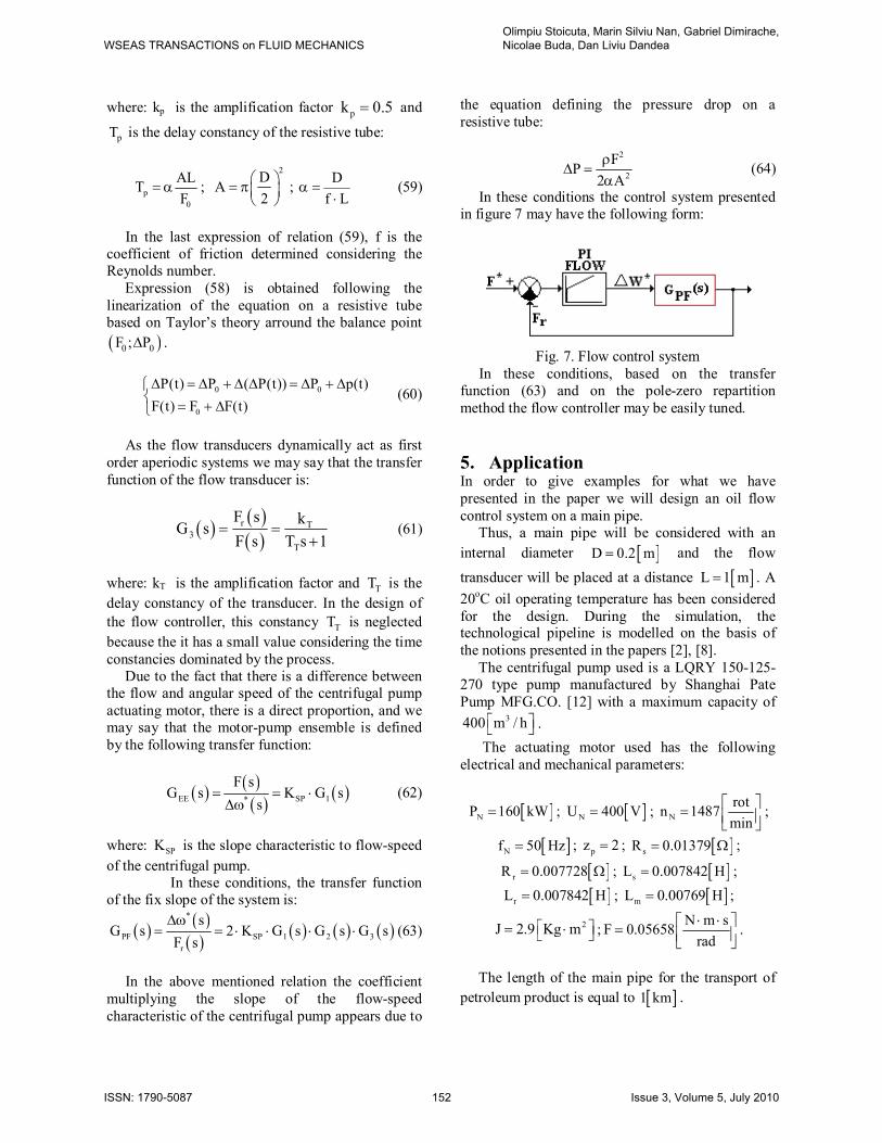
In these conditions the control system presented in figure 7 may have the following form:

Fig. 7. Flow control system

In these conditions, based on the transfer function (63) and on the pole-zero repartition method the flow controller may be easily tuned. 5. Application In order to give examples for what we have presented in the paper we will design an oil flow control system on a main pipe. Thus, a main pipe will be considered with an internal diameter D 0.2 m and the flow transducer will be placed at a distance L 1 m . A 20oC oil operating temperature has been considered for the design. During the simulation, the technological pipeline is modelled on the basis of the notions presented in the papers [2], [8]. The centrifugal pump used is a LQRY 150-125-270 type pump manufactured by Shanghai Pate Pump MFG.CO. [12] with a maximum capacity of

3400 m / h . The actuating motor used has the following electrical and mechanical parameters:

NP 160 kW ; NU 400 V ; Nrotn 1487min

;

Nf 50 Hz ; pz 2 ; sR 0.01379 ;

rR 0.007728 ; sL 0.007842 H ;

rL 0.007842 H ; mL 0.00769 H ;

2J 2.9 Kg m ; N m sF 0.05658rad

.

The length of the main pipe for the transport of petroleum product is equal to 1 km .



For the design of the controllers from speed control systems the following values of the constancies *

d1T and *d2T have been used:

*

d1T 1 msec ; *d2T 7.5 msec . (65)

Following the tuning of flow controller based on the described procedure in this paper the following values of the coefficients defining the controller have been obtained: qK 5 ; qT 0.0005 sec .

For the simulation of flow control system with the modification of the speed of the centrifugal pump, for the flow *F different values have been imposed, respectively 50, 80, 150 and 200 [m3/h]. The simulation of the control system has used Matlab-Simulink software, and following the simulation the following graphs have been obtained:

Fig. 8 Time proportioned flow variation

Fig. 9 Pressure drop variation on the pipe

Fig. 10 Motor’s speed time variation

Considering all the previously presented it is observed that the control system has a very good dynamics.



6 Conclusions The used concepts and ideas in the design of the control system presented in the paper may be used and developed for other types of flow control systems as well. Because of the real advantages of the sensorless control of speed and good dynamic control performances of the new control system we may say that implementing and using the system is a real advantage. References: [1] C. Schauder (1992) Adaptive Speed Identification

for Vector Control of Induction Motors without Rotational Transducers, IEEE Trans. Ind. Applicat., Vol.28, no.5, pp. 1054-1061

[2] D. Matko, G. Geiger, M.A. Kunc (2006) Modelling of Pipelines in State – Space, Proc. WSEAS Int. Conf. on Fluid Mechanics and Aerodinamics, pp.174 – 179.

[3] F.K. Benra, H.J. Dohmen (2008) Numerical and Experimental Investigation of the Flow in a Centrifugal Pump Stage, Proc. WSEAS Int. Conf. on Fluid Mechanics, pp.71 – 76.

[4] H. Kubota, K. Matsuse and T.Nakano (1990) New Adaptive Flux observer of Induction Motor for Wide Speed range Motor Drives, in Proc. Int. Conf. IEEE IECON, pp. 921-926

[5] I. Al-Bahaddly (2007) Energy Saving with Variable Speed Drives in Industry Application, Proc. WSEAS Int. Conf. on Circuits, Systems, Signal and Telecommunication, pp.53 – 58.

[6] I. Lie, V. Tiponut, I. Bogdanov, S. Ionel, C.D. Caleanu (2007) The Development of CPLD – Based Ultrasonic Flow meter, Proc. WSEAS Int. Conf. on Circuits, pp.190 – 193.

[7] M. Popov, Hyperstability of Control Systems (1973) Springer Verlag, New York

[8] M. Tertisco (1991) Continuous Industrial Automation, Teaching and Pedagogical Publishing Group, Bucharest.

[9] O. Stoicuţa, T.Pana (2009) Design and stability study of an induction motor vector control system with extended rotor –flux and rotor - resistance Gopinath observer, ELECTROMOTION, Lile, France, pp.1-8.

[10]O. Stoicuta.,H. Campian, T. Pana (2005) Transfer Function Determination for Vector-Controlled Induction Motor Drives, ELECTROMOTION, Lausanne, Switzerland, pp. 316-321.

[11]O. Stoicuta, M.S. Nan, G. Dimirache, N. Buda, D. Dandea (2010) Research regarding the design of an new transport pipe flow control

system, Proc. WSEAS Int. Conf. Application of Electical Engineering, AEE’10.

[12] *** www.ptcm.com



research regarding the use of new systems to control … regarding the use of new systems to control...

Documents