RESEARCH REPORT SERIES(Statistics - #2006-6)

Statistical Properties of

Model-Based Signal Extraction Diagnostic Tests

Tucker McElroy

Statistical Research DivisionU.S. Census Bureau

Washington, DC 20233

Report Issued: June 5, 2006

Disclaimer: This report is released to inform interested parties of ongoing research and to encourage discussion of work

in progress. The views expressed are those of the author and not necessarily those of the U.S. Census Bureau.

Statistical Properties of Model-Based Signal Extraction Diagnostic

Tests

Tucker McElroy

U.S. Census Bureau

Abstract

A model-based diagnostic test for signal extraction was first described in Maravall (2003), and

this basic idea was modified and studied in Findley, McElroy, and Wills (2004). The paper at

hand improves on the latter work in two ways: central limit theorems for the diagnostics are

developed, and two hypothesis-testing paradigms for practical use are explicitly described. A

further modified diagnostic provides an interpretation of one-sided rejection of the Null Hypoth-

esis, yielding general notions of “over-modeling” and “under-modeling.” The new methods are

demonstrated on two U.S. Census Bureau time series exhibiting seasonality.

Keywords. ARIMA model, Seasonal adjustment, Filtering, Central limit theorem.

Disclaimer This paper is released to inform interested parties of ongoing research and to encour-

age discussion of work in progress. The views expressed are those of the author and not necessarily

those of the U.S. Census Bureau.

1 Introduction

The model-based approach to signal extraction, while elegant and optimal under certain condi-

tions, is still in need of a suite of diagnostics capable of identifying the quality of the procedure.

Certainly, model inadequacy – assessed for example through Ljung-Box statistics – will imply a poor

signal estimate, but the inverse statement need not hold, i.e., goodness of model fit, as indicated

through standard ARIMA model diagnostics, need not indicate the goodness of the corresponding

signal extraction method. This is the case, because deviations of the data from the fitted ARIMA

model, deemed harmless according to standard ARIMA goodness-of-fit measures, may cause seri-

ous problems from the perspective of accurately estimating an ambient signal, e.g., a seasonal or

a trend. One reason for this phenomenon is that the maximum likelihood procedure for fitting

ARIMA models typically fits the best model to the data, without regard to the postulated com-

ponent models. This is the case even with a structural components approach (Harvey 1989), since

1

poorness of fit of the component models is only assessed in a global sense. Thus, for some series,

the quality of the signal extraction may be in doubt and can be assessed through various spectrum

diagnostics, assuming a frequency-based characterization of signal and noise – see Findley, Monsell,

Bell, Otto, and Chen (1998) and Soukup and Findley (1999).

In the seasonal adjustment program SEATS (Gomez and Maravall, 1997) a series of diagnostics,

based on quantifying the variation in estimated signals, have been in use for several years, and

have recently been documented in Maravall (2003) and associated with a statistical test. These

model-based seasonal adjustment diagnostics for over- and under-smoothing of the seasonal com-

ponent were later adapted for finite sample signal extraction in Findley, McElroy, and Wills (2004).

The basic concept is to measure the variation of an estimated signal – assessed through a variance

estimate of the appropriately “differenced” signal extraction – and compare this quantity to what

we would expect if our model were true. Thus, extreme values of variation, relative to a benchmark

computed from a hypothesized model, would indicate model inadequacy with respect to the com-

ponent model for the desired signal. For example, an extreme diagnostic computed for the trend

would indicate poor modelling of the low frequencies, since these constitute the spectral domain of

trends.

Further, one may distinguish between intra- and inter-component variation. The former is con-

cerned with the expected second-order structure of an estimated signal, measured through its

auto-covariance function. The latter treats the expected variation across estimated components,

measured through the cross-covariance function. When modified slightly, these diagnostics can

be interpreted as weighted measures of model fit, placing more weight on discrepancies between

model and truth that occur at frequencies pertinent to the signal of interest. With this spectral

interpretation the diagnostics of Maravall (2003) seem to be a fairly natural measure.

Mathematically, the diagnostics can typically be viewed as a quadratic form in the differenced

data. This simple structure facilitates a finite sample description in terms of mean and variance of

the statistic, as well as the analysis of the asymptotic behavior. A full knowledge of the covariance

structure of the signal error process is required, which can easily be obtained via a matrix-based

approach to filtering (McElroy, 2005). This paper generalizes the results of Findley, McElroy, and

Wills (2004), describing the statistical behavior with full rigor. First the background notation

for signal extraction is developed, and two hypothesis testing schemas are described. In the next

section we discuss the statistical properties of the diagnostics, as well as their applications. These

methods are demonstrated on two time series in the following section. Proofs are contained in an

Appendix.

2

1.1 Signal Extraction Notations

Since we wish to consider mean square optimal signal extraction from a finite sample, we follow

the approach of McElroy (2005). Consider a nonstationary time series Yt that can be written as

the sum of two possibly nonstationary components St and Nt, the signal and the noise:

Yt = St + Nt (1)

Following Bell (1984), we let Yt be an integrated process such that Wt = δ(B)Yt is stationary,

where B is the backshift operator and δ(z) is a polynomial with all roots located on the unit circle

of the complex plane (also, δ(0) = 1 by convention). This δ(B) is the differencing operator of the

series, and we assume it can be factored into relatively prime polynomials δS(z) and δN (z) (i.e.,

polynomials with no common zero), such that

Ut = δS(B)St Vt = δN (B)Nt (2)

are stationary time series. Note that included as special cases are δS = 1 and/or δN = 1, in which

case either the signal or the noise or both are stationary. We let d be the order of δ, and dS and

dN are the orders of δS and δN ; since the latter operators are relatively prime, δ = δS · δN and

d = dS + dN .

For example, the noise could be a nonstationary seasonal with trend plus irregular signal (or

nonseasonal), in which case δS(z) could be (1− z)2, and the noise has differencing operator δN (z) =

1 + z + z2 + · · · z11 for monthly data. This is the appropriate setup for seasonal adjustment, in

which case we are interested in estimating St.

As in Bell and Hillmer (1988), we assume Assumption A of Bell (1984) holds on the component

decomposition, and we treat the case of a finite sample with t = 1, 2, · · · , n. Assumption A states

that the initial d values of Yt, i.e., the variables Y1, Y2, · · · , Yd, are independent of {Ut} and {Vt}.For a discussion of the implications of this assumption, see Bell (1984) and Bell and Hillmer (1988).

A further assumption that we make is that {Ut} and {Vt} are uncorrelated time series.

Now we can write (2) in a matrix form, as follows. Let ∆ be an n − d × n matrix with entries

given by ∆ij = δi−j+d (the convention being that δk = 0 if k < 0 or k > d). The matrices ∆S and

∆N have entries given by the coefficients of δS(z) and δN (z), but are n − dS × n and n − dN × n

dimensional respectively. This means that each row of these matrices consists of the coefficients of

the corresponding differencing polynomial, horizontally shifted in an appropriate fashion. Hence

W = ∆Y U = ∆SS V = ∆NN

3

where Y is the transpose (denoted by Y ′) of (Y1, Y2, · · · , Yn), and W , U , V , S, and N are also

column vectors. It follows from the equation

Wt = δN (B)Ut + δS(B)Vt (3)

that we need to define further differencing matrices ∆N and ∆S with row entries given by the

coefficients of δN (z) and δS(z) respectively, which are n−d×n−dS and n−d×n−dN dimensional.

Then we can write down the matrix version of (3):

W = ∆NU + ∆SV (4)

We will be interested in estimates of U and V . The minimum mean squared error linear signal

extraction estimate is Ut, which can be expressed as some linear function of the differenced data

vector W ; putting this together for each time t, we obtain the various rows of a matrix F :

U = FW.

We note that the various rows of F differ (unlike in the bi-infinite filtering case), since only a finite

number of Yt’s are available to filter. The last row of F , for example, corresponds to the concurrent

filter, i.e., a one-sided filter used to extract a signal at “time present.”

For any random vector X, let ΣX denote its covariance matrix. With these notations in hand, we

can now state the signal extraction formulas, which are given in Proposition 1 of McElroy (2005):

U = ΣU∆′NΣ−1

W W = FW (5)

which implicitly defines F . Later on, it will be necessary to discuss spectra. For a stationary

process {Xt}, we use fX(λ) to denote its spectral density; this is related to the autocovariance

matrix ΣX by the formula

[ΣX ]jk =12π

∫ π

−πfX(λ)ei(j−k)λ dλ.

More generally, for any bounded positive symmetric function g(λ), we define

[Σ(g)]jk =12π

∫ π

−πg(λ)ei(j−k)λ dλ. (6)

This will be called the ACF matrix of g, and is always Toeplitz. Note our use of 2π, which differs

from some authors.

1.2 Hypothesis Testing Framework

In this paper, we must make a distinction between a specified model for W – whose covariance

matrix is denoted ΣW – and the true covariance matrix for W , based on the true underlying

4

Data Generating Process (DGP) – denoted by ΣW . The perspective is that a specified ΣW –

determined either via ad hoc principles or through maximum likelihood estimation – will differ

from ΣW . However, we assume that at least the differencing operators δS and δN have been

correctly ascertained. Note that, denoting the true spectral density by fW , ΣW = Σ(fW ).

Let us denote a particular choice of model – our Null model – by ΣW , the model’s covariance

matrix under the Null Hypothesis. This Null Hypothesis is simply a particular choice of AR and

MA polynomials that determine the ARMA model for Wt. We further suppose that a specification

of ΣW in turn determines ΣU and ΣV , which will be the case if we obtain the models for S and

N via a canonical decomposition (Hillmer and Tiao, 1982) of the model for Y . In this fashion,

we can explore model inadequacy directly through the choice of ΣW , without explicitly accounting

for ΣU and ΣV ; this also covers the approach of SEATS, which uses the canonical decomposition

technique.

The alternative space consists of any other ARMA model for Wt, including different polynomial

orders, coefficients, and innovation variance. However, the differencing polynomials δS and δN are

the same for both the Null and Alternative models. Note that ΣW could in practice be determined

by ARMA coefficient parameter estimates, which we will then treat as fixed rather than random.

This perspective is motivated by the difficulty of stipulating a random quantity for the Null model.

So our testing framework is

H0 : ΣW = ΣW (7)

H1 : ΣW 6= ΣW

As a second testing paradigm, we consider the “innovation-free” version of (7), where the data’s

covariance matrix is essentially assumed to have unit innovation variance σ2a:

H†0 : ΣW/σa

= ΣW/σa(8)

H†1 : ΣW/σa

6= ΣW/σa

This second paradigm is motivated by the observation that the signal extraction filters are de-

termined completely by the ARMA coefficients, and do not depend on the innovation variance.

Note that for both testing paradigms, the alternative space has no particular directionality that is

naturally associated with it. Thus, there is no basis for one-sided tests with these null and alter-

native hypotheses. We later argue that the spectrum provides an appropriate tool for determining

directionality of rejection of H0, in the context of estimating signals. The basic idea is, model inad-

equacy can be assessed in the context of signal extraction by measuring an estimated component’s

deviance from H0 in an appropriate spectral range; this will allow for meaningful one-sided tests.

5

Findley, McElroy, and Wills (2004) presented a test statistic for any differenced signal U based

on its sample variance. That work claimed asymptotic normality of the test statistic under H0;

in Section 2, this claim is verified under two different scenarios. We also expand the basic sample

variance results to include sample autocovariances and crosscovariances. Section 3 discusses various

applications of these asymptotic results to testing, power, and suitable interpretations for rejection

and non-rejection of H0. We consider two examples for which the diagnostic gives interesting

results. Proofs are contained in an Appendix.

2 Theoretical Results

We present several test statistics, which can all be written as a symmetric quadratic form in the

differenced data W = (W1, W2, · · · ,Wn−d)′. First we define two main examples of signal extraction

diagnostics, and then we discuss their asymptotic behavior in a theorem. Next, we extend to the

case that the data’s innovation variance is estimated, and examine the asymptotics of a modified

diagnostic for this scenario.

2.1 Autocovariance and Crosscovariance Diagnostics

The basic idea of SEATS’s diagnostic for over- and under-adjustment is to measure the second-

order properties of estimated signal and noise, and compare to what we should expect if our model

is true. Then any gross disparities lead us to rejection of our model, and hence of our filtering as

well. As a first step, consider the test statistic given by the sample second moment of Ut, compared

to its expectation under H0; this quantity is not scale-invariant, so it is then normalized by its

standard error under H0. The formula is given by

An =U′U

n=

W ′Σ−1W ∆NΣUΣU∆

′NΣ−1

W W

n, (9)

which follows from (5). Note that the normalization of n does not match the length of U , which

is n− dS . Later, we will normalize the diagnostics, so that the choice of n versus n− dS becomes

irrelevant. One way to measure the sample autocovariance is to insert a lag matrix in the inner

product above. Let L be an n − dS dimensional square matrix with Lij = 0 unless i = j + 1 and

Lj+1,j = 1. Then

An(h) =U′LhU

n=

W ′Σ−1W ∆NΣULhΣU∆

′NΣ−1

W W

n(10)

for any 0 ≤ h < n gives the lag h autocovariance estimate. It is necessary to symmetrize this

matrix in theoretical formulas, so let

Lsym, h =12(Lh + L

′h).

6

Then the autocovariance estimate can be rewritten as

An(h) =U′Lsym, hU

n=

W ′Σ−1W ∆NΣULsym, hΣU∆

′NΣ−1

W W

n. (11)

Notice that this is a symmetric quadratic form in the differenced data W . For the crosscovariance

between U and V , which are of length n− dS and n− dN respectively, it is necessary to trim the

longer vector. Without loss of generality, suppose that dN < dS so that V is longer. It will be

shown later that the first values (as opposed to the last values) of the vector should be trimmed;

this is achieved via the formula

[0 1n−dS] V = [0 1n−dS

] ΣV ∆′SΣ−1

W W. (12)

Here 1n−dSdenotes the n−dS dimensional identity matrix, and 0 denotes a zero matrix of dimension

n− dS × dS − dN . We then take the inner product with U , inserting the lag matrix Lh:

Cn(h) =W ′Σ−1

W

(∆NΣULh[0 1]ΣV ∆

′S

)symΣ−1

W W

n(13)

The [0 1] matrix has the same dimensions as in (12) above. Note that we have symmetrized the

interior matrix. In this manner, the autocovariance and crosscovariance diagnostics are defined.

2.2 Fixed Parameters Case

Suppose that an ARMA model for Wt is completely specified. When following the Hilmer and

Tiao (1982) approach, it may be possible to obtain a canonical decomposition and thereby derive

ARMA models for Ut and Vt. Or if a structural approach is adopted (Harvey 1989), the models for

Ut and Vt could be specified directly. Note that model-based filters do not depend on innovation

variance (see McElroy 2005), but the mean squared errors of the estimates they produce do, and

the mean and variance of the test statistics will as well. The following theorem summarizes the

small sample properties and asymptotics of An(h) and Cn(h), and is appropriate for the testing

paradigm described by (7). Since both of these statistics have the form Q(W ) = W′BW/n for

some symmetric matrix B, we describe the results in terms of Q(W ). For the asymptotic results,

the various spectral densities need to satisfy a certain smoothness condition. Writing γg(h) for the

hth coefficient of g(λ) in the Fourier basis, we say that g is in the space C1 if

∑

h

|h||γg(h)| < ∞.

It is a standard fact that C1 ⊂ C1([−π, π]), the space of once continuously differentiable functions

on [−π, π].

7

Theorem 1 Assume that Assumption A holds on the component decomposition (1) and that {Ut}and {Vt} are independent. If the third and fourth cumulants of the true DGP of Wt are zero, then

the true mean and variance of Q(W ) are given by

EQ(W ) =1n

tr(BΣW ) (14)

V arQ(W ) =2n2

tr((BΣW )

2)

where tr denotes the trace of a matrix. The matrix B is either Σ−1W ∆NΣULsym, hΣU∆

′NΣ−1

W or

Σ−1W

(∆NΣULh[01]ΣV ∆

′S

)symΣ−1

W depending on whether we are considering autocovariances or

crosscovariances. Moreover, if fW , fW , fU , fV ∈ C1, and if fW is strictly positive with 1/fW ∈ C1,

then the mean and variance have the following limiting behavior as n →∞:

EQ(W ) → 12π

∫ π

−πg(λ) fW (λ) dλ

nV arQ(W ) → 22π

∫ π

−πg2(λ) f2

W (λ) dλ

where g(λ) = f2U (λ)|δN (e−iλ)|2 cos(hλ)/f2

W (λ) in the autocovariance case, and in the crosscovari-

ance case

g(λ) = fU (λ)fV (λ)(δN (e−iλ)δS(eiλ)e−ihλ + δN (eiλ)δS(e−iλ)eihλ

)/2f2

W (λ).

Also, if the process {Wt} satisfies either condition (B) or (HT) referenced in the Appendix, then

the following Central Limit Theorem holds as n →∞:

τn =√

n(Q(W )− EQ(W ))√

nV arQ(W )L=⇒ N (0, 1)

Remark 1 The assumptions are common to the literature on convergence of functionals of the

periodogram (see Taniguchi and Kakizawa (2000)), and do not seem very stringent. A linear Gaus-

sian process satisfies the cumulant condition as well as condition (B). A non-Gaussian stationary

process (with third and fourth order cumulants zero) that is a causal filter of white noise with C1

spectral density satisfies condition (HT). If we formulate an ARMA model for Wt and apply the

canonical decomposition, then necessarily fW , fU , fV ∈ C1. If ARMA is the correct specification,

then clearly fW ∈ C1 as well. The data need not be Gaussian, but must “look” Gaussian up to

fourth order. The programs X13−AS and TRAMO−SEATS provide diagnostics for the presence

of skewness and kurtosis; if skewness and kurtosis are present, the asymptotic distribution may not

have unit variance.

In order to compute the mean and standard error, it is necessary to assume something about

the DGP, such as that provided by the hypothesis H0. In practice, one could use Theorem 1 as

follows: estimate a model for Wt, and declare this to be the Null model described by ΣW , now

8

viewed as having fixed (nonrandom) parameters. If we have a method for uniquely determining fU

and fV from fW (such as the canonical decomposition approach of Hillmer and Tiao (1982)), then

an α probability of Type I error has the interpretation that an independent replicate, i.e., a series

with DGP given by ΣW , with filters computed without re-estimation of model parameters, would

have probability α of falsely rejecting H0. Note that if we were to re-estimate model parameters

for the independent replicate, H0 would no longer be true for that series (since its DGP given by

ΣW would in general differ from maximum likelihood estimates of that DGP).

Hence, this gives the following application for power studies: if a model ΣW is fitted to a series,

then we set the Null model equal to the estimate, and simulate series (assuming some distribution

compatible with our assumptions) from H0; then, since the Null model is correct for each simulation,

we construct model-based filters based on H0, without re-estimating model parameters for each

simulation. The quantiles of the test statistic’s empirical distribution function form estimates of

the testing procedure’s critical values. Next, selecting any other choice of ΣW , we can compute

filters and test statistics based on the false Alternative model, and compute the probability of Type

II error for a given critical value, thus obtaining a power surface.

2.3 Estimated Innovation Variance Case

We now focus on a scenario where all of the model parameters are specified except for the

innovation variance σ2ε ; hence, our results will be appropriate for the second hypothesis testing

paradigm (8). For example, if it is thought that the data can be modelled with an airline model,

and we wish to test whether the signal extraction using a (.6, .6) airline model is reasonable, i.e.,

Wt = (1−B)(1−B12)Yt = (1− .6B)(1− .6B12)εt,

then we should estimate the innovation variance σ2ε from the data, assuming that the other two

parameters are correct. In this section, we describe how to modify the diagnostics to accommodate

this situation.

What is known then is the “innovation free” version of the covariance matrix of W , denoted by

ΣW/σε. Likewise ΣU/σε

is based on the model for Ut with innovation variance given in units of σ2ε .

Hence we can write the signal extraction matrix for U as F = ΣU/σε∆′NΣ−1

W/σε, which no longer

requires knowledge of σε. In fact, we can write (for the autocovariance diagnostic)

B = Σ−1W/σε

∆NΣU/σεLsym,hΣU/σε

∆′NΣ−1

W/σε.

A similar formula holds for the cross-covariance case. Thus, we can compute Q(W ) without prior

knowledge (or estimation) of σε, but its mean and variance do depend on the innovation variance.

9

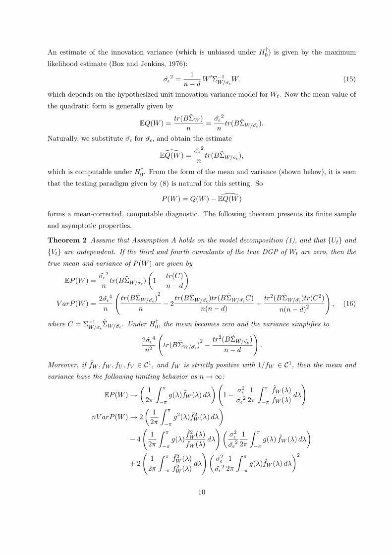
An estimate of the innovation variance (which is unbiased under H†0) is given by the maximum

likelihood estimate (Box and Jenkins, 1976):

σε2 =

1n− d

W ′Σ−1W/σε

W, (15)

which depends on the hypothesized unit innovation variance model for Wt. Now the mean value of

the quadratic form is generally given by

EQ(W ) =tr(BΣW )

n=

σε2

ntr(BΣW/σε

).

Naturally, we substitute σε for σε, and obtain the estimate

EQ(W ) =σε

2

ntr(BΣW/σε

),

which is computable under H†0. From the form of the mean and variance (shown below), it is seen

that the testing paradigm given by (8) is natural for this setting. So

P (W ) = Q(W )− EQ(W )

forms a mean-corrected, computable diagnostic. The following theorem presents its finite sample

and asymptotic properties.

Theorem 2 Assume that Assumption A holds on the model decomposition (1), and that {Ut} and

{Vt} are independent. If the third and fourth cumulants of the true DGP of Wt are zero, then the

true mean and variance of P (W ) are given by

EP (W ) =σε

2

ntr(BΣW/σε

)(

1− tr(C)n− d

)

V arP (W ) =2σε

4

n

(tr(BΣW/σε

)2

n− 2

tr(BΣW/σε)tr(BΣW/σε

C)n(n− d)

+tr2(BΣW/σε

)tr(C2)

n(n− d)2

), (16)

where C = Σ−1W/σε

ΣW/σε. Under H†

0, the mean becomes zero and the variance simplifies to

2σε4

n2

(tr(BΣW/σε

)2 − tr2(BΣW/σε

)n− d

).

Moreover, if fW , fW , fU , fV ∈ C1, and fW is strictly positive with 1/fW ∈ C1, then the mean and

variance have the following limiting behavior as n →∞:

EP (W ) →(

12π

∫ π

−πg(λ)fW (λ) dλ

) (1− σ2

ε

σε2

12π

∫ π

−π

fW (λ)fW (λ)

dλ

)

nV arP (W ) → 2(

12π

∫ π

−πg2(λ)f2

W (λ) dλ

)

− 4

(12π

∫ π

−πg(λ)

f2W (λ)

fW (λ)dλ

) (σ2

ε

σε2

12π

∫ π

−πg(λ) fW (λ) dλ

)

+ 2

(12π

∫ π

−π

f2W (λ)

f2W (λ)

dλ

)(σ2

ε

σε2

12π

∫ π

−πg(λ)fW (λ) dλ

)2

10

with g as in Theorem 1. Also, if the process {Wt} satisfies either condition (B) or (HT) referenced

in the Appendix, then the following Central Limit Theorem holds as n →∞:

√n

(P (W )− EP (W ))√nV arP (W )

L=⇒ N (0, 1) (17)

Remark 2 The variance of P (W ) under H†0 must be estimated by the following:

n V arP (W ) = 2σε4

(tr(BΣW/σε

)2

n− tr2(BΣW/σε

)n(n− d)

)

It is easily checked that this converges in probability to the limit of nV arP (W ), and so may be

substituted into (17) by Slutsky’s Theorem. Thus we compute the statistic

τ †n =√

nP (W )√

n V arP (W ),

which is asymptotically standard normal under H†0 .

Remark 3 If we treat σε and the ARMA parameters as fixed, then

σε2ΣW/σε

= ΣW .

It follows that

P (W )|H†

0= Q(W )− 1

ntr(BΣW ) = Q(W )− EQ(W )|H0

n V arP (W )|H†

0= 2

(tr(BΣW )

2

n− tr2(BΣW )

n(n− d)

)

= nV arQ(W )|H0 − 2tr2(BΣW )n(n− d)

.

Hence in this case, P (W ) has less variability than Q(W ). Thus it is easier to reject H†0 than H0

when the model parameters come from estimates that are treated as fixed. This makes sense, since

H0 implies H†0.

The application and interpretation of Theorem 2 is similar to that discussed for Theorem 1. For

an estimated model, an independent replicate with innovation variance re-estimated would falsely

reject H†0 with probability α, given the appropriate critical value. Note that in this case, the “unit-

innovation variance” DGP for the replicate and the model used for the filters exactly coincide,

so H†0 is true. If instead we were to re-estimate the non-innovation variance parameters for the

replicate, then we would obtain parameter estimates that would in general be different from the

DGP parameters, and thus H†0 would be false. So only the innovation variance is to be re-estimated

in this interpretation.

11

3 Applications and Extensions

A primary objective of this work is to determine the asymptotics of diagnostics introduced in

Findley, McElroy, and Wills (2004). Theorems 1 and 2 provide ways to compute asymptotic power

for the procedures, under a two-sided alternative. However, it is desirable to obtain an interpretation

for positive versus negative values of the diagnostic, so as to obtain a sensible one-sided test. In

addition, we want rejection of the Null Hypothesis to give us meaningful information about how

our model is incorrect for signal extraction, and how it might be modified.

In this section, we discuss a modification of the autocovariance diagnostic that facilitates such

interpretations. Then we demonstrate the properties of the diagnostic on two seasonal time series.

Finally, we explore the question of redundancy: how correlated are the various diagnostics with

one another when the model is correct? Can all this information be consolidated? We note that

even though the original over- and under-adjustment diagnostics of Maravall (2003) and later

Findley, McElroy, and Wills (2004) sought to address the issue of over- and under-smoothing of a

signal extraction component, in fact these diagnostics assess over- and under-modeling of various

components. This distinction is further clarified and explored in this section.

3.1 Over- and Under-Modeling

From the results of the previous section, we know that the autocovariance diagnostic, under some

conditions, converges in probability to

12π

∫ π

−πf2

U (λ)|δN (e−iλ)|2 cos(hλ)fW (λ)f2

W (λ)dλ =

12π

∫ π

−πfU (λ)

fS(λ)fY (λ)

cos(hλ)fW (λ)fW (λ)

dλ.

So An(0) is a measure of model discrepancy – fW /fW – weighted by the function fUfS/fY . Ob-

serve that the function fS/fY is an appealing weighting function, since it is bounded between 0

and 1 for all frequencies, and attains its minimum (zero) at “noise” frequencies and its maximum

(one) at “signal” frequencies, i.e., those frequencies that are roots of δN (e−iλ) and δS(e−iλ) respec-

tively. Such a weighting function fS/fY fully weights model discrepancy from truth fW /fW at

signal frequencies, but disregards discrepancies occurring at the noise frequencies. Unfortunately,

the asymptotic limit of An(0) does not provide such a weighting function; it weights the model

discrepancy by fUfS/fY , and the function fU can destroy the interpretation of fully weighting

signal frequencies. This is because fU can be quite general: for example, it can be flat or even have

a high-pass form 1 + ρ2 − 2ρ cosλ for ρ close to one (this would be problematic for a trend signal,

where low frequencies should receive more weight).

12

We propose the following modified diagnostic, which will correspond to the desired weighting

scheme fS/fY :

An(h) =W

′Σ−1

W ∆N (ΣULh)sym∆′NΣ−1

W W

n,

where (ΣULh)sym = (ΣULh + L′hΣU )/2. This can be written in the form Q(W ) as in Section 2,

with a matrix B = Σ−1W ∆NΣULhsym∆

′NΣ−1

W . The same types of theoretical results (Theorems 1

and 2) apply to An, but now the appropriate function g is defined by

g(λ) = fU (λ)|δN (e−iλ)|2 cos(hλ)f−2W (λ).

Thus we have the convergence

An(h) P−→ 12π

∫ π

−πcos(hλ)

fS(λ)fY (λ)

fW (λ)fW (λ)

dλ.

In addition,

EAn(h)|H0 =1n

tr(BΣW )|H0 →12π

∫ π

−πcos(hλ)

fS(λ)fY (λ)

dλ,

so we have

An(h)− EAn(h)|H0

P−→ 12π

∫ π

−πcos(hλ)

fS(λ)fY (λ)

(fW (λ)fW (λ)

− 1

)dλ. (18)

This is the numerator of the normalized modified diagnostic. We form a variance normalization

along the lines of Theorem 1 (use equation (14) with the above choice of B), and call the normalized

quantity τ . That is,

τ =An(h)− EAn(h)√

V ar(An(h)).

Note that we have developed this modified diagnostic with the testing paradigm H0 in mind, but

a similar treatment can easily be developed for H†0 .

Given these asymptotics, we can offer the following interpretation. Let us refer to the range of

frequencies where fS is high relative to fY as the “spectral range” of the signal. Now if fW > fW

in the spectral range of the signal, then (18) is positive and the diagnostic is too large. But if

fW < fW in the spectral range, then (18) is negative and the diagnostic is too small. Now when

fW < fW in a spectral band, the model is too chaotic for those frequencies since it assigns too

much variation there. This will be referred to as “over-modeling.” Conversely, fW > fW indicates

the model is too stable, as it assigns too little variation at the signal frequencies. This will be

referred to as “under-modeling.” Outside the spectral range of the signal these interpretations are

less meaningful, since the weighting function will dampen the effect of model discrepancies. These

observations can be used to form a meaningful one-sided testing procedure. First we summarize

13

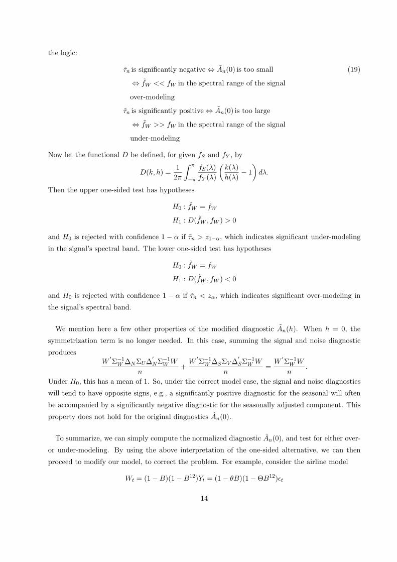
the logic:

τn is significantly negative ⇔ An(0) is too small (19)

⇔ fW << fW in the spectral range of the signal

over-modeling

τn is significantly positive ⇔ An(0) is too large

⇔ fW >> fW in the spectral range of the signal

under-modeling

Now let the functional D be defined, for given fS and fY , by

D(k, h) =12π

∫ π

−π

fS(λ)fY (λ)

(k(λ)h(λ)

− 1)

dλ.

Then the upper one-sided test has hypotheses

H0 : fW = fW

H1 : D(fW , fW ) > 0

and H0 is rejected with confidence 1− α if τn > z1−α, which indicates significant under-modeling

in the signal’s spectral band. The lower one-sided test has hypotheses

H0 : fW = fW

H1 : D(fW , fW ) < 0

and H0 is rejected with confidence 1 − α if τn < zα, which indicates significant over-modeling in

the signal’s spectral band.

We mention here a few other properties of the modified diagnostic An(h). When h = 0, the

symmetrization term is no longer needed. In this case, summing the signal and noise diagnostic

producesW

′Σ−1

W ∆NΣU∆′NΣ−1

W W

n+

W′Σ−1

W ∆SΣV ∆′SΣ−1

W W

n=

W′Σ−1

W W

n.

Under H0, this has a mean of 1. So, under the correct model case, the signal and noise diagnostics

will tend to have opposite signs, e.g., a significantly positive diagnostic for the seasonal will often

be accompanied by a significantly negative diagnostic for the seasonally adjusted component. This

property does not hold for the original diagnostics An(0).

To summarize, we can simply compute the normalized diagnostic An(0), and test for either over-

or under-modeling. By using the above interpretation of the one-sided alternative, we can then

proceed to modify our model, to correct the problem. For example, consider the airline model

Wt = (1−B)(1−B12)Yt = (1− θB)(1−ΘB12)εt

14

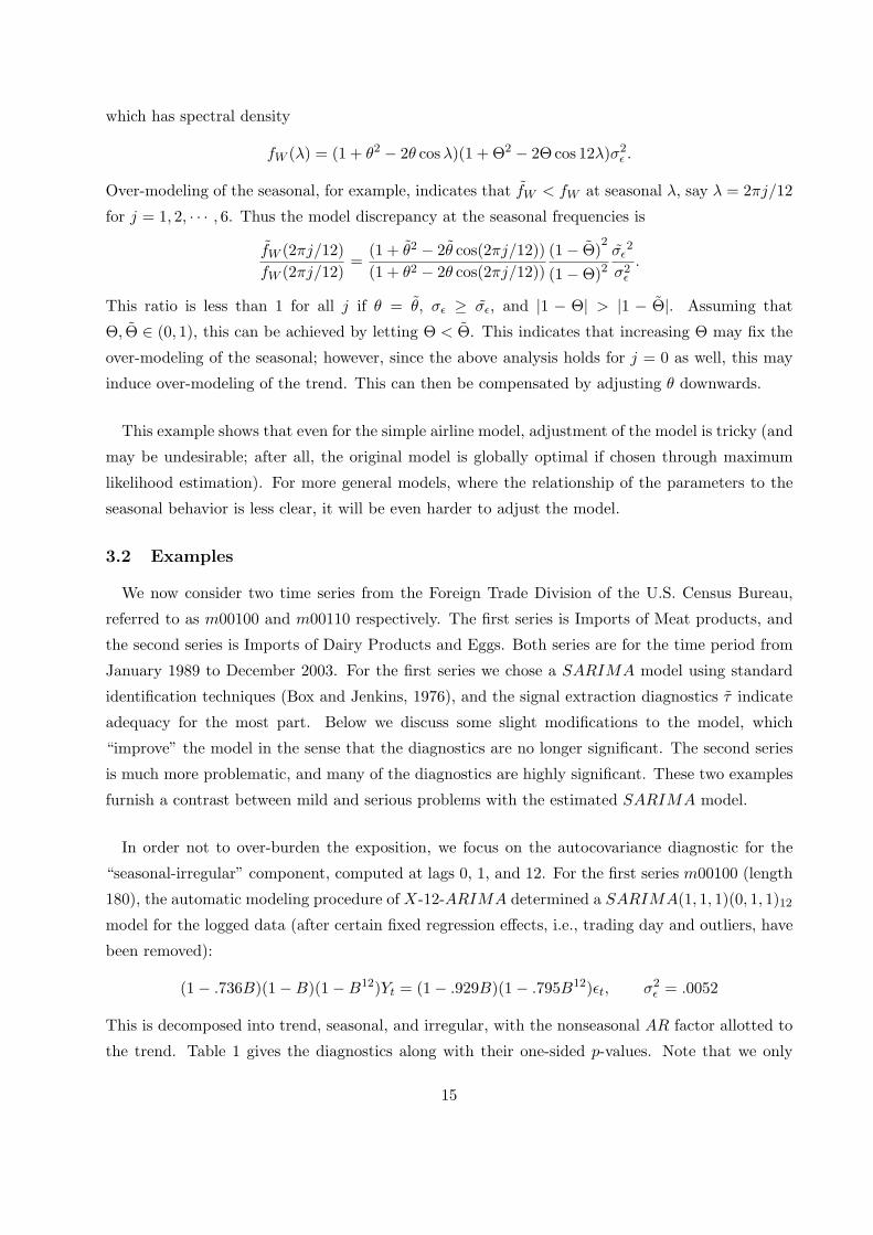
which has spectral density

fW (λ) = (1 + θ2 − 2θ cosλ)(1 + Θ2 − 2Θ cos 12λ)σ2ε .

Over-modeling of the seasonal, for example, indicates that fW < fW at seasonal λ, say λ = 2πj/12

for j = 1, 2, · · · , 6. Thus the model discrepancy at the seasonal frequencies is

fW (2πj/12)fW (2πj/12)

=(1 + θ2 − 2θ cos(2πj/12))(1 + θ2 − 2θ cos(2πj/12))

(1− Θ)2

(1−Θ)2σε

2

σ2ε

.

This ratio is less than 1 for all j if θ = θ, σε ≥ σε, and |1 − Θ| > |1 − Θ|. Assuming that

Θ, Θ ∈ (0, 1), this can be achieved by letting Θ < Θ. This indicates that increasing Θ may fix the

over-modeling of the seasonal; however, since the above analysis holds for j = 0 as well, this may

induce over-modeling of the trend. This can then be compensated by adjusting θ downwards.

This example shows that even for the simple airline model, adjustment of the model is tricky (and

may be undesirable; after all, the original model is globally optimal if chosen through maximum

likelihood estimation). For more general models, where the relationship of the parameters to the

seasonal behavior is less clear, it will be even harder to adjust the model.

3.2 Examples

We now consider two time series from the Foreign Trade Division of the U.S. Census Bureau,

referred to as m00100 and m00110 respectively. The first series is Imports of Meat products, and

the second series is Imports of Dairy Products and Eggs. Both series are for the time period from

January 1989 to December 2003. For the first series we chose a SARIMA model using standard

identification techniques (Box and Jenkins, 1976), and the signal extraction diagnostics τ indicate

adequacy for the most part. Below we discuss some slight modifications to the model, which

“improve” the model in the sense that the diagnostics are no longer significant. The second series

is much more problematic, and many of the diagnostics are highly significant. These two examples

furnish a contrast between mild and serious problems with the estimated SARIMA model.

In order not to over-burden the exposition, we focus on the autocovariance diagnostic for the

“seasonal-irregular” component, computed at lags 0, 1, and 12. For the first series m00100 (length

180), the automatic modeling procedure of X-12-ARIMA determined a SARIMA(1, 1, 1)(0, 1, 1)12

model for the logged data (after certain fixed regression effects, i.e., trading day and outliers, have

been removed):

(1− .736B)(1−B)(1−B12)Yt = (1− .929B)(1− .795B12)εt, σ2ε = .0052

This is decomposed into trend, seasonal, and irregular, with the nonseasonal AR factor allotted to

the trend. Table 1 gives the diagnostics along with their one-sided p-values. Note that we only

15

have a sensible interpretation for one-sided tests for the modified diagnostic τ . According to τ , the

model is adequate, whereas τ and τ † indicate under-modeling at lag 12. It is interesting that the

lag 0 diagnostics are all negative, although not significantly so. Thus we might proceed with the

diagnosis that there is mild under-modeling. Since Θ controls the seasonal movement, it can be

adjusted downwards to generate more variation at the seasonal frequencies, which increases fW in

the signal’s spectral band. In Table 2, we present the diagnostics obtained by fixing Θ = .6 (instead

of at the MLE value of .795) and keeping the other parameters the same (alternatively, one could

re-estimate the innovation variance with these fixed parameter values). Experimentation with other

values of Θ yields similar results: the under-modeling of the seasonal-irregular component is abated.

Table 1. Diagnostics with p-values for m00100.

Diagnostic Lag 0 p-value Lag 1 p-value Lag 12 p-value

τ -1.01 .155 -.15 .441 2.43 .007

τ † -1.57 .058 -.16 .438 2.62 .004

τ -1.03 .152 1.27 .101 1.07 .143

Table 2. Diagnostics with p-values for m00100, Θ fixed at .6

Diagnostic Lag 0 p-value Lag 1 p-value Lag 12 p-value

τ .08 .468 .19 .426 1.55 .061

τ † .10 .459 .20 .420 1.55 .061

τ -.70 .241 1.09 .137 .35 .363

The second series m00110 (length 180) in logs is modeled with a SARIMA(2, 0, 1)(0, 1, 1)12

model (after removing a temporary change and outlier regression effect):

(1− 1.065B + 0.209B2)(1−B12)Yt = (1− 0.528B)(1− 0.982B12)εt, σ2ε = .0085

The model coefficients were estimated using X-12-ARIMA. We note that convergence of the

maximum likelihood parameter estimation procedure was somewhat slow, and the diagnostics for

the seasonal-irregular are highly significant, as shown in Table 3. In the lag 0 case, the sign of τ

and τ † actually differ from τ . Restricting our attention to τ , we conclude from the significantly

negative lag zero diagnostic, together with (19), that there is over-modeling of the seasonal present.

However, the high value of Θ indicates that little can be done to increase Θ, and instead we may

consider lowering θ. Some experimentation show that this ameliorates the situation, and Table 4

displays results with θ = .2. Even with this low value of θ, some of the τ and τ † diagnostics are

significant (although less so); however, the τ is no longer significant, which is the most important

measure. Of course, another approach might be to adjust the model specification, perhaps to a

SARIMA (1, 1, 1)(0, 1, 1)12 or (0, 1, 1)(0, 1, 1)12.

16

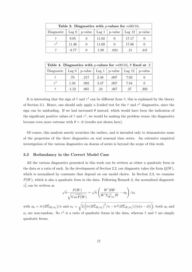
Table 3. Diagnostics with p-values for m00110.

Diagnostic Lag 0 p-value Lag 1 p-value Lag 12 p-value

τ 9.05 0 11.02 0 17.17 0

τ † 11.36 0 11.69 0 17.86 0

τ -3.77 0 1.98 .024 .15 .441

Table 4. Diagnostics with p-values for m00110, θ fixed at .2

Diagnostic Lag 0 p-value Lag 1 p-value Lag 12 p-value

τ .78 .217 2.46 .007 7.02 0

τ † 1.33 .092 2.47 .007 7.84 0

τ -1.52 .065 .24 .467 .27 .393

It is interesting that the sign of τ and τ † can be different from τ ; this is explained by the theory

of Section 3.1. Hence, one should only apply a 2-sided test for the τ and τ † diagnostics, since the

sign can be misleading. If we had increased θ instead, which would have been the indication of

the significant positive values of τ and τ †, we would be making the problem worse; the diagnostics

become even more extreme with θ = .6 (results not shown here).

Of course, this analysis merely scratches the surface, and is intended only to demonstrate some

of the properties of the three diagnostics on real seasonal time series. An extensive empirical

investigation of the various diagnostics on dozens of series is beyond the scope of this work.

3.3 Redundancy in the Correct Model Case

All the various diagnostics presented in this work can be written as either a quadratic form in

the data or a ratio of such. In the development of Section 2.2, our diagnostic takes the form Q(W ),

which is normalized by constants that depend on our model choice. In Section 2.3, we examine

P (W ), which is also a quadratic form in the data. Following Remark 2, the normalized diagnostic

τ †n can be written as√

nP (W )√V arP (W )

=√

n

(W

′BW

W ′Σ−1W/σε

W− a0

)/a1

with a0 = tr(BΣW/σε)/n and a1 =

√2

(tr(BΣW/σε

)2/n− tr2(BΣW/σε

)/(n(n− d))); both a0 and

a1 are non-random. So τ † is a ratio of quadratic forms in the data, whereas τ and τ are simply

quadratic forms.

17

For diagnostics of the form Q(W ), we can easily compute correlations. Given two such normalized

diagnostics for two signals S and S], the correlation is given by

Cov(Q(W ), Q](W ))√V arQ(W )V arQ](W )

=2tr(BΣW B]ΣW )

2√

tr(BΣW )2tr(B]ΣW )

2.

Thus, under H0 we can use this formula to compute the correlation for either τ or τ . We work out

some details for the latter case. The numerator works out to be

2tr

(∆NΣ1/2

U Lsym,hΣ1/2U

′∆′NΣ−1

W ΣW Σ−1W ∆]

NΣ]U

1/2Lsym,kΣ]

U

1/2′

∆]N

′Σ−1

W ΣW Σ−1W

)/n2.

Multiplying by n, it converges to

22π

∫ π

−π|δN (e−iλ)|2fU (λ) cos(hλ)

fW (λ)f2

W (λ)|δN

] (e−iλ)|2f ]U (λ) cos(kλ)

fW (λ)f2

W (λ)dλ.

This can be rewritten as

22π

∫ π

−π

fS(λ)fY (λ)

f ]S(λ)

fY (λ)cos(hλ) cos(kλ)

f2W (λ)

f2W (λ)

dλ.

This combines the weighting functions fS/fY and f ]S/fY . Taking h = k = 0, we see that the

correlation is always non-negative, but is closer to zero when S and S] occupy separate frequency

bands. For example, taking S] = N , the weighting function is fSfN/f2Y .

Note that the positive correlation effect does not imply that a particular diagnostic computed

for signal and noise should have opposite signs. It means that if one diagnostic is higher on another

data set, the other diagnostic will be higher too. This effect is reduced by using the modified

diagnostic, and by taking complementary signals.

4 Conclusion

This paper defines several diagnostics for goodness of signal extraction, and describes their sta-

tistical behavior. The original diagnostics τ and τ † were proposed in Findley, McElroy, and Wills

(2004), although essentially only for the lag zero auto-covariance case. Here we expand the class of

such diagnostics to include other lags and cross-covariance as well, and in addition present a mod-

ified τ that allows for interpretability of the sign. This allows us to conduct meaningful one-sided

tests, and provides some direction for how the model should be changed in order to correct over-

or under-modeling in particular signal frequency bands. We do not claim that it is easy to know

how a given SARIMA model should be altered; but we have tried to demonstrate that τ and τ †

cannot be used reliably to alter a model.

18

Of course, a given model chosen by maximum likelihood should be the best fit for the data,

since it is preferred to other SARIMA models (at least with the same differencing orders) by AIC

or another model comparison criterion. However, the Gaussian maximum likelihood procedure

looks for a model fW that is close to the truth fW in an average sense, over all the frequencies.

This is because the quantity W′Σ−1

W/σεW/(n− d) occurring in the likelihood function converges in

probability to

σ2ε

12π

∫ π

−π

fW (λ)fW (λ)

dλ.

One way to view Gaussian maximum likelihood estimation, is that it is a procedure that seeks out

fW from a model class such that the above quantity is close to σ2ε . Of course, this formula only

holds asymptotically. The diagnostics τ examine model discrepancy fW /fW over a range of “signal

frequencies,” which is achieved by integrating against the weighting function fS/fY ; in contrast,

maximum likelihood estimation uses the weight fY /fY = 1. This can be seen as addressing the

issue of global versus local fit, in a spectral sense. That is, a model fW may be good as an overall

fit to fW , considering all frequencies at once, but may be a poor fit at some particular band of

frequencies. By sacrificing the global fit, a model can arguably be improved locally, i.e., at the

signal and noise frequency bands.

In practice, a plethora of signal extraction diagnostics can be produced, and it is reasonable to

think that there may be some redundancy in them. For τ and τ , correlations between various

auto-covariance diagnostics can be calculated for each example, and in this fashion any redundancy

can be assessed. Future work will focus on large-scale empirical investigations of these statistics.

5 Appendix: Proofs

We first delineate a proposition that establishes asymptotic normality of a certain special class of

quadratic forms. Being of interest in its own right, this result can be applied to an approximation

of the diagnostics considered in this paper. We consider a stationary process {Wt}, whose spectral

density is denoted by fW (λ). Given a sample W = {W1,W2, · · · ,Wn}′, we denote the periodogram

by fW (λ):

fW (λ) =1n

∣∣∣∣∣n∑

t=1

Wte−iλt

∣∣∣∣∣2

Then it follows at once that

1n

W ′Σ(g)W =12π

∫ π

−πg(λ) fW (λ) dλ.

The following proposition describes the asymptotics of this quadratic form. Some mild conditions on

the data are required for the asymptotic theory; we follow the material in Taniguchi and Kakizawa

19

(2000, Section 3.1.1). Condition (B), due to Brillinger (1981), states that the process is strictly

stationary and condition (B1) of Taniguchi and Kakizawa (2000, page 55) holds. Condition (HT),

due to Hosoya and Taniguchi (1982), states that the process has a linear representation, and

conditions (H1) through (H6) of Taniguchi and Kakizawa (2000, pages 55 – 56) hold. Neither of

these conditions are stringent; for example, a causal linear filter of a white noise process with fourth

moments satisfies (HT).

Proposition 1 Suppose that the stationary process {Wt} satisfies either condition (B) or (HT).

Let g be any real, even, continuous function on [−π, π]. Then as n → ∞ the following assertions

hold:∫ π

−πg(λ) fW (λ) dλ

P−→∫ π

−πg(λ) fW (λ) dλ

√n

∫ π

−πg(λ)

(fW (λ)− fW (λ)

)dλ

L=⇒ N (0, V )

where the limiting variance V is given by

V = 4π

∫ π

−πg2(λ) f2

W (λ) dλ

+∫ π

−π

∫ π

−πg(λ) g(ω) QW (−λ, ω,−ω) dλ dω

and QW is the tri-spectral density of {Wt}, i.e.,

QW (λ1, λ2, λ3) =∑

t1,t2,t3∈Zexp{−i(λ1t1 + λ2t2 + λ3t3)}CW (t1, t2, t3)

and CW is the fourth-order cumulant function of the process.

Proof of Proposition 1. Since g is real, even, and continuous, the first convergence result

follow at once from Lemma 3.1.1 of Taniguchi and Kakizawa (2000). Note that they define the

periodogram with a 2π factor. 2

We next state and prove several approximation lemmas for the analysis of quadratic forms, which

are of interest in their own right and are used in the proof of Theorem 1.

Lemma 1 Let ∆ be the m− d×m dimensional matrix associated to an order d polynomial δ(z),

given by

∆ij = δj+d−i

where we let δk = 0 if k < 0 or k > d. Then, for m-dimensional Σ(g),

∆Σ(g)∆′= Σ(g · f)

where f(λ) = |δ(e−iλ)|2.

20

Proof of Lemma 1. Based on formula (6), we have(∆Σ(g)∆

′)jk

=∑

l,t

∆jlΣlt(g)∆kt

=12π

∑

l,t

δj+d−lδk+d−t

∫ π

−πg(λ)ei(l−t)λ dλ

=12π

∫ π

−πg(λ)ei(j−k)λ

∑

l

δj+d−le−i(j+d−l)λ

∑t

δk+d−tei(k+d−t)λ dλ

=12π

∫ π

−πg(λ)δ(e−iλ)δ(eiλ)ei(j−k)λ dλ,

which is the jkth entry of the Toeplitz matrix associated to g · f , as desired. 2

For the next three lemmas, we need a concept from Taniguchi and Kakizawa (2000). If we let

γg(j − k) = Σjk(g), then a discrete approximation is given by the Riemann sum

γg(h) =1n

n∑

k=1

g(λk)eihλk

with λk = 2πk/n. In this manner we define the Toeplitz approximation to Σ(g) via

Σjk(g) = γg(j − k).

See Taniguchi and Kakizawa (p. 490, 2000) for related results, which we cite here for easy reference.

It can be shown that

Σ(g) = H∗DH

with Hjk = n−1/2ei2πjk/n and D = diag{g(λ1), · · · , g(λn)}. The ∗ denotes conjugate transpose.

Lemma 2 Let f be a continuous function on [−π, π] in C1, and let Zt and Xt be two sequences of

(possibly correlated) random variables with uniformly bounded second moments. Let Z = (Z1, Z2, · · · , Zn)′

and X = (X1, X2, · · · , Xn)′, and let Σ(f) be n-dimensional. Then

Z′Σ(f)X = OP (1) + Z

′Σ(f)X

as n →∞.

Proof of Lemma 2.

E∣∣∣Z ′

Σ(f)X − Z′Σ(f)X

∣∣∣

≤∑

j,k

E|ZjXk|∣∣Σjk(f)− Σjk(f)

∣∣ ≤ supj

√E[Z2

j ] supk

√E[X2

k ]∑

j,k

∣∣Σjk(f)− Σjk(f)∣∣

using the Cauchy-Schwarz inequality. Now apply Lemma 7.2.9 of Taniguchi and Kakizawa (2000),

which is due to Wahba (1968), noting that boundedness in absolute mean implies that the expression

is bounded in probability. 2

21

Lemma 3 Let g and f be continuous functions on [−π, π] satisfying the same conditions as in

Lemma 2, and suppose that the random variables Zt have uniformly bounded second moments.

Then

Z′Σ(f)Σ(g)Σ(f)Z = OP (1) + Z

′Σ(f2 · g)Z

as n →∞.

Proof of Lemma 3.

Z′Σ(f)Σ(g)Σ(f)Z − Z

′Σ(f2 · g)Z = Z

′(Σ(f)Σ(g)− Σ(f · g))Σ(f)Z (20)

+ Z′ (

Σ(f · g)Σ(f)− Σ(f2 · g))Z

Let X = Σ(f)Z; a fact that we use repeatedly is that X will satisfy the same boundedness properties

as Z, so long as γf is absolutely summable:

Xj =n∑

k=1

Σjk(f)Zk =n∑

k=1

γf (j − k)Zk

X2j =

n∑

k,l=1

γf (j − k)γf (j − l)ZkZl

EX2j ≤

(sup

k

√EZ2

k

)2

supj{

∞∑

k,l=−∞|γf (j − k)||γf (j − l)|}

It is easy to see that the latter supremum is bounded by (∑∞

k=−∞ |γf (k)|)2. So in a like manner,

Y = Σ(g)X has bounded second moments, and we can apply Lemma 2 to Z′Σ(f)Y :

Z′Σ(f)Y = OP (1) + Z

′Σ(f)Y

Now Z′Σ(f)Y = V

′Σ(g)X, where V = Σ(f)Z also has bounded second moments (this follows from

Lemma 7.2.9 of Wahba (1968)). Again we apply Lemma 2, and finally obtain

Z′Σ(f)Σ(g)X = OP (1) + Z

′Σ(f)Σ(g)X;

the advantage of this representation is that Σ(f)Σ(g) = Σ(f · g) follows from the Hermitian form

of these matrices. In a like manner,

Z′Σ(f · g)X = OP (1) + Z

′Σ(f · g)X

by another application of Lemma 2. This shows that the first term on the right hand side of (20) is

OP (1). An analogous argument holds for the second term. Note that we only need that the Fourier

coefficients of f and g are absolutely summable, which follows from the conditions of the Lemma.

2

22

We also wish to consider inverses of Toeplitz matrices. It is clear from the Hermitian form of

Σ(f) that

Σ(f)−1 = H∗D−1H = Σ(1/f)

so long as f is nowhere equal to zero. We can extend Lemma 2 to this case as follows:

Lemma 4 Make the same assumptions as in Lemma 2, and suppose that f is strictly positive.

Then

Z′Σ(f)−1X = OP (1) + Z

′Σ(1/f)X

as n →∞.

Proof of Lemma 4. Use the same proof as Lemma 2, but now apply the result of Liggett (1971),

also found on page 491 and 492 of Taniguchi and Kakizawa (2000). Note that it is necessary that

f be bounded away from zero, so that we avoid division by zero. 2

With these lemmas, we can now prove Theorem 1 for the autocovariance diagnostics; for the

crosscovariances diagnostics, some additional tinkering with the lemmas will be needed.

Proof of Theorem 1. First consider the formulas given in (14); the expectation is immediate,

and the variance formula is standard, assuming that third and fourth order cumulants vanish – see

McCullagh (1987, p. 65). Note that the matrix of the quadratic form Q(W ) must be symmetric;

otherwise this formula for the variance is not true. This explains why we use the “symmetrization”

technique.

For the asymptotic results, we first prove the Central Limit Theorem, and note that the conver-

gences of mean and variance can be proved in an analogous manner, but are actually easier since

the formulas are deterministic. Consider the autocovariance diagnostic first, and let Z = Σ−1W W .

Then

An(h) = OP (1/n) + Z′∆NΣ(f2

U · l)∆′NZ/n

using Lemmas 2 and 3. Here l(λ) = cos(λh) and Lsym,h = Σ(l) (note that l ∈ C1). Applying

Lemma 1,

Z′∆NΣ(f2

U · l)∆′NZ/n = W

′Σ−1

W Σ(f2

U · l · |δN (e−i·)|2)

Σ−1W W/n.

Next, apply Lemma 4 to obtain

An(h) = OP (1) + W′Σ

(f2

U · l · |δN (e−i·)|2 · f−2W

)W.

Now since 1/fW ∈ C1 and C1 is closed under multiplication, it follows that f2U ·l·|δN (e−i·)|2·f−2

W ∈ C1,

and we can apply Lemma 2:

An(h) = OP (1) + W′Σ

(f2

U · l · |δN (e−i·)|2 · f−2W

)W.

23

Now under the additional assumption (B) or (HT), we can apply Proposition 1, since the function

f2U ·l·|δN (e−i·)|2·f−2

W is continuous and even (continuity of each function follows from its summability,

and the product is continuous because fW is strictly positive). This gives a limit theorem

√n

(Q(W )− 1

2π

∫ π

−πg(λ)fW (λ) dλ

)L=⇒ N (0, V ),

where g is defined in the theorem’s statement. Using the convergence for the mean and variance,

the limit result is proved.

Next, consider the cross-covariance diagnostic. Letting Z = Σ−1W W again, apply Lemma 2 several

times to obtain

Z′∆NΣULh[0 1]ΣV ∆

′SZ = OP (1) + Z

′∆NΣ(fU )Lh[0 1]Σ(fV )∆

′SZ.

In forming the approximations Σ, we utilize the dimension n − dS for both ΣU and ΣV . For the

latter matrix, this differs from our former definition, since ΣV is n − dN × n − dN dimensional.

Explicitly,

Σ(fV ) = G∗EG

with Gjk = (n− dS)−1/2ei2πjk/(n−dS) and E = diag{g(λ1), · · · , g(λn−dS), 0, · · · }; λj = 2πj/(n−dS).

It is easy to see that the approximation Lemmas are still valid when we use n−dS instead of n−dN

in the definition of Σ(fV ). For convenience let m = n− dS and calculate as follows:(H Lh [0 1] G∗

)jk

=m∑

t=1

m−1/2e−i2πj(t+h)/mm−1/2ei2π(t+dS−dN )k/m

= m−1e−i2πjh/mei2π(dS−dN )k/mm∑

t=1

e−i2πt(j−k)/m

= δj,ke−i2πj(h−dS+dN )/m

where δj,k is the Kronecker delta (not to be confused with the coefficients of δ(z)). This calculation

illustrates why we needed to modify the definition of Σ(fV ). So the above matrix is n−dS×n−dN

and “diagonal” in the sense that the only nonzero entries occur when the row and column index

are equal. Call this matrix F . Then

Σ(fU )Lh[0 1]Σ(fV ) = H∗C F E G

and C F E is another “rectangular diagonal” matrix, with jth diagonal entry given by

fU (λj)fV (λj)e−iλj(h−dS+dN )

24

so long as j ≤ m. Therefore,

(H∗C F E G)jk

=∑

l,t

m−1/2ei2πjl/mδl,tfU (λl)fV (λl)e−iλl(h−dS+dN )m−1/2e−i2πtk/m

= m−1m∑

t=1

e−i2πt(k−j)/mfU (λt)fV (λt)e−iλt(h−dS+dN ),

which can be viewed as just the jkth entry of a rectangular Toeplitz matrix Σ(fU ·fV ·e−i(h−dS+dN )·).

Applying the random vectors Z′∆N and ∆

′SZ, the inner product is OP (1) away from the form

Z′∆NΣ(fU · fV · e−i(h−dS+dN )·)∆

′SZ,

by applying Lemmas 2 and 3, extended to the rectangular scenario. Finally, we show how the

differencing matrices account for the time delay factor e−i(h−dS+dN )λ:(∆NΣ(fU · fV · e−i(h−dS+dN )·)∆

′S

)jk

=12π

∫ π

−πfU (λ)fV (λ)e−iλ(h−dS+dN )

∑

l

δNj+dN−l

∑t

δSk+dS−te

iλ(l−t) dλ

=12π

∫ π

−πfU (λ)fV (λ)

∑

l

δNj+dN−le

−iλ(j+dN−l)∑

t

δSk+dS−te

iλ(k+dS−t)e−iλ(h−j+k) dλ

=12π

∫ π

−πfU (λ)fV (λ)δN (e−iλ)δS(eiλ)e−iλheiλ(j−k) dλ

= Σjk

(fU · fV · δN (e−i·) · δS(ei·) · e−ih·

),

which can have complex entries. Notice that in order for the delay factors induced by the differencing

matrices to cancel with e−i(h−dS+dN )λ, it is necessary to trim V of its first dS − dN entries, as a

careful examination of our proof will reveal. At this point, we consider the symmetrization of this

form, which amounts to symmetrizing the delay factors δN (e−i·) · δS(ei·) · e−ih·. Apply Lemma 4 to

obtain

Cn(h) = OP (1/n) + W′Σ (g) W/n,

using the fact that 1/fW ∈ C1 as before. From here we apply Proposition 1 and the proof is

complete. 2

Proof of Theorem 2. We begin with the mean and variance calculations.

EP (W ) =tr(BΣW )

n− Eσε

2 tr(BΣW/σε)

n

and

Eσε2 = σε

2tr(Σ−1

W/σεΣW/σε

)

n− d

25

together yield the formula for the mean. For the variance we have

V arP (W ) = V arQ(W )− 2Cov(Q(W ), EQ(W )) + V arEQ(W )

=2n2

tr(BΣW )2 − 4

n2(n− d)tr(BΣW/σε

)tr(BΣW Σ−1W/σε

ΣW )

+2

n2(n− d)2tr2(BΣW/σε

)tr(Σ−1W/σε

ΣW )2,

which is easily manipulated into the stated form. The limiting mean and variance formulas are

justified using the same techniques as in Theorem 1. For the central limit theorem, we note that

P (W ) =1n

W′BW − σε

2

ntr(BΣW/σε

) =1n

W′ [

B − tr(BΣW/σε)Σ−1

W/σε

]W.

Thus P (W ) is a symmetric quadratic form, and the same asymptotic techniques apply to the matrix

B − tr(BΣW/σε)Σ−1

W/σε. Asymptotically, the associated Toeplitz matrix is Σ(g − βσ2

ε /fW ) with

β = σε−2 1

2π

∫ π

−πg(λ)fW (λ) dλ.

Hence P (W ) is asymptotically normal with mean and variance given by

12π

∫ π

−π(g(λ)− βσ2

ε /fW (λ))fW (λ) dλ

n−1 22π

∫ π

−π(g(λ)− βσ2

ε /fW (λ))2f2W (λ) dλ

respectively. It is easily checked that these are identical to the stated expressions for the limit of

the mean and variance. 2

References

[1] Bell, W. (1984) Signal Extraction for Nonstationary Time Series. The Annals of Statistics 12,

646 –664.

[2] Bell, W. and Hillmer, S. (1988) A Matrix Approach to Likelihood Evaluation and Signal

Extraction for ARIMA Component Time Series Models. SRD Research Report No. RR−88/22,

Bureau of the Census.

[3] Box, G. and Jenkins, G. (1976) Time Series Analysis, San Francisco, California: Holden-Day.

[4] Brillinger, D. (1981) Time Series Data Analysis and Theory. San Francisco: Holden-Day.

[5] Findley, D., McElroy, T., Wills, K. (2004) “Diagnostics for ARIMA-Model-Based Seasonal Ad-

justment,” 2004 Proceedings of the American Statistical Association [CD-ROM]: Alexandria,

VA.

26

[6] Findley, D. F., Monsell, B. C., Bell, W. R., Otto, M. C. and Chen, B. C. (1998) New Capabil-

ities and Methods of the X-12-ARIMA Seasonal Adjustment Program. ” Journal of Business

and Economic Statistics, 16 127–177 (with discussion).

[7] Gomez, V. and Maravall, A. (1997) Program SEATS Signal Extraction in ARIMA Time Series:

Instructions for the User (beta version: June 1997), Working Paper 97001, Ministerio de

Economıa y Hacienda, Dirrection General de Analysis y Programacion Presupuestaria, Madrid.

[8] Harvey, A. (1989) Forecasting, Structural Time Series Models and the Kalman Filter. Cam-

bridge: Cambridge University Press.

[9] Hillmer, S. and Tiao, G. (1982) An ARIMA-Model-Based Approach to Seasonal Adjustment.

Journal of the American Statistical Association 77, 377, 63 – 70.

[10] Hosoya, Y., and Taniguchi, M. (1982) A central limit theorem for stationary processes and the

parameter estimation of linear processes. Annals of Statistics 10, 132–153.

[11] Liggett, W.S. (1971) On the asymptotic optimality of spectral analysis for testing hypotheses

about time series. Annals of Mathematical Statistics 42, 1348–1358.

[12] Maravall, A. (2003) A Class of Diagnostics in the ARIMA-Model-Based Decomposition of a

Time Series. Memorandum, Bank of Spain.

[13] McCullagh, P. (1987) Tensor Methods in Statistics, London: Chapman and Hall.

[14] McElroy, T. (2005) Matrix Formulas for Nonstationary Signal Extraction. SRD Research Re-

port No. 2005/04, Bureau of the Census.

[15] Soukup, R. and Findley, D. (1999) On the spectrum diagnostics used by X-12-ARIMA to

indicate the presence of trading day effects after modeling or adjustment. Proceedings of the

Business and Economic Statistics Section, 144–149, American Statistical Association. Also

www.census.gov/pub/ts/papers/rr9903s.pdf

[16] Taniguchi, M. and Kakizawa, Y. (2000) Asymptotic Theory of Statistical Inference for Time

Series, New York City, New York: Springer-Verlag.

[17] Wahba, G. (1968) On the distribution of some statistics useful in the analysis of jointly sta-

tionary time series. Annals of Mathematical Statistics 39, 1849–1862.

27