reserve requirements for price and financial stability ... · pdf filereserve requirements for...
TRANSCRIPT

Reserve Requirements for Price and FinancialStability: When Are They Effective?∗
Christian Glocker and Pascal TowbinBanque de France
Reserve requirements are a prominent policy instrumentin many emerging countries. The present study investigatesthe circumstances under which reserve requirements are anappropriate policy tool for price or financial stability. We con-sider a small open-economy model with sticky prices, finan-cial frictions, and a banking sector that is subject to legalreserve requirements and compute optimal interest rate andreserve requirement rules. Overall, our results indicate thatreserve requirements can support the price stability objectiveonly if financial frictions are important and lead to substantialimprovements if there is a financial stability objective. Con-trary to a conventional interest rate policy, reserve require-ments become more effective when there is foreign currencydebt.
JEL Codes: E580, E520, F410, G18.
1. Introduction
Reserve requirements are a prominent policy instrument in manyemerging countries. China, for example, raised its reserve require-ments six times in 2010, while moving interest rates only once (seeKashyap and Stein 2012). The Central Bank of Turkey recently low-ered its policy interest rate and increased reserve requirements atthe same time. Among policymakers, reserve requirements are under
∗The authors would like to thank Carl Walsh and Robert King, MirkoAbbritti, Fabian Eser, and participants at the Banque de France seminar andthe IJCB conference in Ottawa for helpful comments and discussions. The viewsexpressed in this paper do not necessarily reflect those of the Banque de Franceor the Eurosystem. Author contact: Banque de France, 31 rue Croix des petitschamps, 75001 Paris, France. Tel: +33 (0) 1 42 92 33 88, +33 (0) 1 42 92 26 66,E-mail: [email protected], [email protected]
65

66 International Journal of Central Banking March 2012
discussion both as a financial stability tool—in particular, in order todeal with volatile capital flows—and as an unconventional monetarypolicy tool for price stability—in particular, when interest rate policyis constrained by the zero lower bound or an exchange rate objec-tive.1 The main objective of reserve requirements varies substantiallyacross countries and over time, and it is not always easy to iden-tify the main purpose (Gray 2011). The Central Bank of Malaysiarecently announced that changes in reserve requirements only serve afinancial stability objective, whereas the interest rate is used for pricestability (see Central Bank of Malaysia 2011). In Turkey, the centralbank considers the interest rate as the main instrument for pricestability, with a secondary role for financial stability, and reserverequirements as the main instrument for financial stability, with asecondary role for price stability (Basci 2010). Until 1993, the BancoCentral do Brasil used heterogeneous reserve requirements acrossregions in order to foster growth in poorer regions by facilitatingcredit supply there (see Carvalho and Azevedo 2008 and Maia deOliveira Ribeira and de Holanda Barbosa 2005). Other countriesuse reserve requirements both for price and financial stability, andthe respective weights vary.2 Using reserve requirements for multiplepurposes has both advantages and disadvantages: On the one hand,a setting where reserve requirements respond to price and financialdevelopments can lead to better outcomes as it increases the degreesof freedom; on the other hand, a separation of tasks might increasetransparency and facilitate communication.
The main aim of the present paper is to analyze under whichcircumstances reserve requirements are effective as an additionalmonetary policy tool to achieve price stability or as a macropruden-tial tool to achieve financial stability. To that purpose we consider asmall open-economy model with sticky prices, financial frictions, and
1In addition, reserve requirements serve also as a source of fiscal revenue andas a tool for liquidity management; see Goodfriend and Hargraves (1983) fora description on how the use of reserve requirements in the United States hasevolved over time.
2Montoro and Moreno (2011) survey the use of reserve requirements in LatinAmerica. Geiger (2008) and Goodfriend and Prasad (2006) discuss monetarypolicy in China, including the use of reserve requirements. The InternationalMonetary Fund (2010) and Moreno (2011) provide an overview on how reserverequirements are used as a macroprudential tool.

Vol. 8 No. 1 Reserve Requirements 67
a banking sector that is subject to legal reserve requirements. Apartfrom the interest rate, the central bank sets reserve requirementsand varies them in response to economic conditions.
Our analysis on the effectiveness of reserve requirements focuseson three key dimensions. The first dimension is the financial struc-ture of the economy. We start from an economy without financialfrictions and then add a financial accelerator mechanism, first withdomestic currency debt and finally with foreign currency debt. Thesecond dimension is the objective of the central bank. We assumethat the central bank receives an exogenous mandate from the gov-ernment in the form of a loss function it has to minimize. In thefirst setting, the central bank aims to minimize a weighted aver-age of the variability of output and inflation. In the second setting,the variability of loans enters additionally. The additional variableintends to capture an intrinsic motivation of the central bank to con-tain credit fluctuations, beyond their effect on price stability. Thecentral bank follows log-linear instrument rules and chooses the reac-tion coefficients that minimize the respective loss function. The thirddimension is operational and captures the type of variables that enterthe instrument rule. In the most general case, both the interest rateand reserve requirements respond to fluctuations in output, inflation,and credit. We consider more restrictive settings, where the policyinstruments respond only to a subset of variables or remain con-stant, compute the relative losses, and analyze interactions betweenthe two instruments.
We start by showing that the transmission of discretionarychanges in reserve requirements depends importantly on other mon-etary arrangements. In the traditional textbook description, changesin the reserve requirements affect the money multiplier and therebymoney supply and, if there are nominal rigidities, real activity.The textbook analysis assumes that the central bank keeps basemoney constant. But if monetary authorities target interest ratesor exchange rates, they accommodate reserve requirement changesautomatically through an endogenous expansion of the monetarybase. In that case, the main transmission channel builds on the inter-est rate differential between the interest rates on loans and reserves.If the remuneration of reserves is below the market rate, an increasein reserve requirements acts as a tax on banks and widens the spreadbetween lending and deposit rates. This can lead to a rise in lending

68 International Journal of Central Banking March 2012
rate and a subsequent decline in investment, but also to a declinein the deposit rate. Everything else fixed, the decline in the depositrate triggers an exchange rate depreciation and capital outflows, butalso an increase in consumption. The overall effect on total demandand inflation is therefore ambiguous.
We initially analyze an economy where the central bank onlycares about the variability of output and inflation and no financialfrictions are present. As supply shocks move output and inflation inopposite directions, an additional instrument in the form of reserverequirements could, in principle, improve the output-inflation trade-off. In our simulations, however, we find the gains to be negligi-ble. The finding can be related to the mechanism described above:with an interest rate rule, changes in reserve requirements tendto move investment and consumption in opposite directions. If weadd a financial accelerator as in Bernanke, Gertler, and Gilchrist(1999), the gains from using reserve requirements are larger. Adapt-ing reserve requirements to economic conditions can alleviate move-ments in the external finance premium. Reserve requirements areparticularly effective if firms borrow in foreign currency. Differentfrom an increase in the policy rate, a raise in reserve requirementsgenerates a depreciation and thereby a decline in firm equity, whichamplifies the effect of reserve requirements through balance sheeteffects. Gains are even larger if the central bank has an explicit finan-cial stability objective and aims to contain fluctuations in creditin addition to output and prices. Adjusting only the interest rateincreases the volatility of the three target variables substantially.Overall our results therefore indicate that reserve requirements cansupport the price stability objective only if financial frictions areimportant and lead to substantial improvements if there is a finan-cial stability objective and debt is denominated in foreign currency.Regarding the interaction between the two instruments, a separationof tasks, where the interest rate responds to fluctuations in out-put and inflation and reserve requirements to fluctuations in loans,appears advantageous, as stabilization losses are small in compari-son to a setting where both instruments respond to all variables andthe setting is considerably simpler.
Most of the more recent literature that studies the use of reserverequirements as a policy tool dates back to the period betweenthe 1980s and the early 1990s and focuses on advanced economies.
Vol. 8 No. 1 Reserve Requirements 69
Over the last twenty years, reserve requirements have been losingimportance as a monetary policy instrument in advanced economiesand there has been little new research on the topic. Fama (1980) andRomer (1985) focus on the microeconomic aspects and analyze theincidence of reserve requirements under different institutional set-tings. Baltensperger (1982) and Horrigan (1988) employ ISLM-typemodels to study the effect of reserve requirements on price and out-put stability. Siegel (1981) analyzes the effect of reserve requirementson price stability in a real model. Since the financial crisis, reserverequirements have received new attention. Kashyap and Stein (2012)analyze how reserve requirements can be used as an additional finan-cial stability tool and act as a Pigouvian tax in a partial equilibriummodel, but they do not consider the real economy and the conse-quences of price stickiness explicitly. Recent papers that study theconsequences of reserve remuneration are also relevant (Curdia andWoodford 2011, Ireland 2011) but different in focus, as they studyunconventional monetary policy at the zero lower bound.
In emerging-market economies, reserve requirements continue toplay an important role. Most research on the use of reserve require-ments in emerging economies has been empirical and focuses on theimpact of reserve requirements on interest spreads and bank profits(see, for instance, Carvalho and Azevedo 2008, Cerda and Larrain2005, Gomez 2007, Ocampo and Tovar 2003, Souza Rodrigues andTakeda 2004, and Vargas et al. 2010). The general conclusion fromthese studies is that increases in reserve requirements raise interestspreads and lower bank profits. However, the studies do not allowdrawing direct conclusion on the macroeconomic, general equilib-rium consequences of reserve requirements. There are also a fewtheoretical studies on the use of reserve requirements in emerg-ing economies. Reinhart and Reinhart (1999) use a variant of theDornbusch overshooting model to examine the effects of changesin reserve requirements on the exchange rate. Edwards and Vegh(1997) discuss the use of reserve requirements as a stabilizationtool in a stylized open-economy model, but they do not considerits interaction with monetary policy and the gains that derive fromusing reserve requirements as an additional instrument. Recently, afew central banks that use reserve requirements have built medium-sized dynamic stochastic general equilibrium (DSGE) models of therespective economies that feature reserve requirements (see Prada
70 International Journal of Central Banking March 2012
Sarmiento 2008 for Colombia and Bokan et al. 2009 for Croatia).In contrast to the present paper, these papers do not provide anexplicit evaluation regarding the gains of using reserve requirementsas an additional policy instrument and how the gains vary with eco-nomic circumstances. The paper is also related to the papers whichfind that interest rate policy is less effective in stabilizing the econ-omy when there is foreign currency debt (for example, Choi andCook 2004, Elekdag and Tchakarov 2007, Towbin and Weber 2011).We complement these studies by finding that reserve requirementsbecome more effective with foreign currency debt, in contrast toconventional monetary policy.
More generally, our study also contributes to the recent litera-ture that analyzes the interaction of monetary and macroprudentialpolicies (Bean et al. 2010, Cecchetti and Kohler 2010, Cecchettiand Li 2005, Darracq Paries, Sørensen, and Rodriguez-Palenzuela2011, Kannan, Rabanal, and Scott 2009). All of the cited studiesare closed-economy models, have a prominent role for the housingsector or bank capital, and focus on advanced economies.
In the remainder, section 2 details model and calibration.Sections 3 and 4 discuss the main results and extensions and section5 concludes.
2. The Model
The core of the model is a relatively standard small open-economymodel with investment, sticky prices, and a financial acceleratormechanism. In addition, household savings have to be intermediatedthrough banks in order to reach firms. Banks make loans to entre-preneurs to finance their capital stock. Banks are subject to reserverequirements set by the government.3 Households consume a bun-dle of home and foreign goods and have access to an internationallytraded bond.
2.1 The Banking Sector
Banks attract funding from households and lend to entrepreneurs.For ease of exposition, we analyze the tasks of lending and funding
3We therefore assume that there are no other means of external finance.Possibilities to circumvent banks would obviously weaken the effects of reserverequirements.

Vol. 8 No. 1 Reserve Requirements 71
separately and consider lending units and deposit units. Households’savings are remunerated at the deposit rate, while deposit units lendto lending units at the (risk-free) interbank rate. Lending units makerisky loans to entrepreneurs.4
2.2 Deposit Units
Deposit units operate in perfectly competitive input and output mar-kets. They collect deposits from households and rent a fraction tolending units on the interbank market and keep the rest as reserveswith the central bank. Profits accrue to households since they arethe owners of the deposit units.
Deposit unit j collects deposits Dt(j) from households and paysa deposit interest rate iDt (j). The bank has two possibilities to usethe deposits. It allocates a fraction 1 − ςt(j) of deposits to lend-ing in the interbank market and earns a gross return equal to iIBt .The remaining fraction of funds Rest(j) = ςt(j)Dt(j) is put into anaccount at the central bank, which is remunerated at the reserve rateiRt . The bank optimally chooses the composition of its assets, takinginto account the minimum reserve requirement ratio ςMP
t imposedby the monetary authority. The balance sheet of the deposit unitreads
Rest(j) + DIBt (j) = Dt(j), (1)
where DIBt (j) = (1 − ςt(j))Dt(j) is interbank lending. Deposit units
face convex costs in holding reserves Gςt(j)
Gςt(j) = ψ1
(ςt(j) − ςMP
t
)+
ψ2
2(ςt(j) − ςMP
t
)2, (2)
where ψ1 and ψ2 are cost function parameters. The first linear termdetermines steady-state deviations from the required reserve ratio.Holding excess reserves may generate some benefits, for example,because it reduces the costs of liquidity management. In addition, thecentral bank may impose a fee for not fulfilling the reserve require-ment. Both motivations would imply ψ1 < 0. The quadratic term
4An alternative would be to consider banks that collect savings and lend atthe same time. The opportunity cost of attracting an additional unit of depositwould then correspond to the interbank rate.

72 International Journal of Central Banking March 2012
with ψ2 > 0 guides the dynamics around the steady state. There areseveral motivations for such convex costs. First, the benefits fromholding excess reserves may decline because of decreasing returnsto scale. Second, the central bank may punish large negative devi-ations from its target with a larger penalty rate and phase out theremuneration of excess reserves at the same time.5
The profit maximization problem of a bank is
max{ςt(j),Dt(j)}
DivSt (j) (3)
subject to equation (2), and dividends (DivSt ) are given by
DivSt (j) =
[(1 − ςt(j))iIBt + ςt(j)iRt − iDt (j) − Gς
t(j)]· Dt(j). (4)
The first-order conditions of the optimization problem are
−[(
iIBt − iRt)
+ ψ1]
= ψ2(ςt(j) − ςMP
t
)(5)
iDt (j) =[(1 − ςt(j))iIBt + ςt(j)iRt − Gς
t(j)]. (6)
Equation (5) determines banks’ actual reserve ratio. It is decreas-ing in the spread between the interbank rate and the reserve rate andincreasing in the required reserve ratio ςMP
t . Equation (6) shows thatthe deposit rate is a weighted average of the rates received from lend-ing and reserve holdings, net of operating costs. The interest ratedifferential iIBt − iRt ≥ 0 represents the opportunity costs depositunits face by investing part of their assets in reserves. Reserverequirements therefore act as a tax on the banking system. Anincrease in the monetary authority’s target value of reserve require-ments increases the opportunity costs. As a consequence, the spreadbetween deposit and interbank rates rises.
2.2.1 Lending Units
Lending units do not interact with households. They are not sub-ject to reserve requirements, as they finance themselves through the
5One could also imagine that positive and negative deviations from the tar-get rate are asymmetric: Positive deviations generate small benefits and neg-ative deviations generate large costs. However, in a linearized setting such aspecification would be equivalent to ours.

Vol. 8 No. 1 Reserve Requirements 73
interbank market and do not hold any deposits from households.Lending units operate in perfectly competitive input and outputmarkets. They obtain funds from deposit units (DIB
t ) at the cost ofthe interbank rate and supply loans to entrepreneurs at the lend-ing rate (iLt ). The amount of interbank lending always equals thestock of loans supplied. The interaction between lending units andentrepreneurs is modeled by means of the financial contract as inBernanke, Gertler, and Gilchrist (1999).
2.2.2 Equilibrium in the Financial Sector
Equilibrium in the financial sector implies that ςt(j) = ςt since,due to equation (5), all deposit units face the same interbank andreserve interest rates as well as the same reserve requirement ratio.Moreover, equation (6) implies that once all banks have chosen thesame level of the reserve requirement ratio, they will henceforth allset the same deposit rate: iDt (j) = iDt . Based on these equilibriumconditions, the following consolidated financial sector balance sheetemerges:
Lt = (1 − ςt)Dt. (7)
Aggregate nominal reserves ςtPtDt correspond to the monetarybase in our model, as households do not hold cash. Taking intoaccount reserve remuneration, real seignorage revenue TS
t is
TSt = ςtDt −
iRt−1
πtςt−1Dt−1.
All seignorage revenue is redistributed as a lump-sum transfer tohouseholds.
2.3 The Household Sector
There is a continuum of households. In a given period householdsderive utility from consumption Ct and disutility from working(ht). Their instant utility function is u(Ct, ht) = lnCt − Ψh1+φ
t
1+φ .Consumption is a Cobb-Douglas bundle of home CH
t and foreignCF
t goods: Ct ∝ (CHt )γ(CF
t )1−γ . The resulting price index readsPt = (PH
t )γ(PFt )1−γ . Households can invest their savings in real
74 International Journal of Central Banking March 2012
deposits Dt and foreign nominal bonds Bt, evaluated at the nominalexchange St. Because of limited capital mobility, acquiring foreignbonds entails a small holding cost ψB
2 (St
PtBt)2.6 By supplying labor,
households receive labor income Wtht. In addition, they receive grossinterest payments on their deposits iDt−1Dt−1, interest payments onforeign bonds i∗t−1StBt−1, dividends from deposit units DivS
t andintermediate goods producers DivR
t , and lump-sum transfers Tt fromthe government.
PtCt + PtDt + StBt = iDt−1Pt−1Dt−1 + i∗t−1StBt−1 + PtWtht
+ Pt
∑j∈{S,R}
Div jt + PtTt +
ψB
2Pt
(St
PtBt
)2
(8)
Households discount instant utility with β. They maximize theirexpected lifetime utility function subject to the budget constraint,which leads to the familiar optimality conditions:
1 = EtΛt,t+1iDt
πt+1
1 − ψBSt
PtBt = Et
[Λt,t+1
i∗tπt+1
St+1
St
]Wt = Ψhφ
t Ct,
where the stochastic discount factor is given by Λt,t+k = βk Ct
Ct+kand
πt = Pt/Pt−1 is the gross inflation rate.
2.4 Capital Goods Producers
Capital goods producers build the capital stock, which is soldto entrepreneurs. They purchase the previously installed capitalstock net of depreciation from enterpreneurs and combine it withinvestment goods to produce the capital stock for the next period.
6The assumption ensures stationarity in small open-economy models (Schmitt-Grohe and Uribe 2003).
Vol. 8 No. 1 Reserve Requirements 75
Investment goods have the same composition as final consumptiongoods. Capital is subject to quadratic adjustment costs accordingto χ
2 ( It
Kt−1− δ)2Kt−1, where δ is the depreciation rate of capital.
The parameter χ captures the sensitivity of changes in the price ofcapital to fluctuations in the investment to capital ratio.
The market price of capital is denoted by Qt. The optimizationproblem is to maximize the present discounted value of dividendsby choosing the level of new investment It. Since the optimizationproblem is completely static, it reduces to
maxIt
[(Qt − 1)It − χ
2
(It
Kt−1− δ
)2
Kt−1
]. (9)
The maximization problem yields the following capital sup-ply curve: Qt = 1 + χ( It
Kt−1− δ). Finally, the aggregate capital
stock evolves according to the following law of motion: Kt =(1 − δ)Kt−1 + It.
2.5 Entrepreneurs
Entrepreneurs are the critical link between intermediate goods pro-ducers and capital goods producers. They purchase capital from thecapital goods producers at the beginning of the period and resell atthe end of the period. They rent it to intermediate goods producersat rental rate zt. The structure of this part of the model is the sameas in Bernanke, Gertler, and Gilchrist (1999) and we postpone thedetails to appendix 1.
Entrepreneurs finance their capital purchases out of their networth Nt and with bank loans from bank lending units. We considertwo cases: in the first case, the loan from the lending unit is denom-inated in domestic currency QtKt = Nt + Lt. In the second case,the loan is denominated in foreign currency QtKt = Nt + StL
∗t . We
interpret the foreign currency case as an approximation for finan-cial dollarization, i.e., an economy where domestic banks (whichare subject to reserve requirements) offer only loans in foreigncurrency.
The interaction between entrepreneurs and bank lending unitsis characterized by an agency problem: entrepreneurs’ projects faceidiosyncratic shocks that are not publicly observable and they have

76 International Journal of Central Banking March 2012
an incentive to underreport their earnings. Lenders can verify theidiosyncratic shock at a cost. The optimal financial contract deliversthe following key equation that links the spread between the aggre-gate expected real return on capital Etr
Kt+1 and the risk-free lending
rate to the entrepreneurs’ leverage:
QtKt = f
(Etr
Kt+1
iIBt /Etπt+1
)Nt, with f ′(·) > 0. (10)
Equation (10) shows that the external finance premium EtrKt+1
iIBt /Etπt+1
increases with the share of debt in total financing. The entrepre-neur’s real return on capital is given by
rKt =
zt + Qt(1 − δ)Qt−1
, (11)
where zt is the real rental cost of capital.7
With a probability 1 − ν, entrepreneurs leave the market andconsume their net worth. They are replaced by new entrepreneurswho receive a small transfer g from the departing entrepreneurs.Aggregate net worth is given by the following expression:
Nt = νVt + (1 − ν)g, (12)
where Vt denotes the net worth of surviving entrepreneurs. Differ-ent from Bernanke, Gertler, and Gilchrist (1999), but in line withGertler, Gilchrist, and Natalucci (2007), we assume that the lend-ing rate is fixed in nominal terms in the respective currency. In thedomestic currency case, the net worth of surviving entrepreneurs is
Vt = (1 − μ)rKt Qt−1Kt−1 − iLt−1
Pt−1
PtLt−1, (13)
7Equation (11) takes into account that in a model with investment adjust-ment costs and incomplete capital depreciation, one has to differentiate betweenthe entrepreneur’s return on capital (rK
t ) and the rental rate on capital (zt).The return on capital depends on the rental rate as well as on the deprecia-tion rate of capital, adjusted for asset price valuation effects (i.e., variations inQt/Qt−1).

Vol. 8 No. 1 Reserve Requirements 77
where the term μ reflects the deadweight cost associated with imper-fect capital markets (see Bernanke, Gertler, and Gilchrist 1999 forfurther details) and iLt is the state-contingent nominal lending ratespecified in the optimal financial contract (see Bernanke, Gertler,and Gilchrist 1999 and appendix 1). Combining equations (12) and(13) yields a dynamic equation for aggregate net worth.
In the scenario where entrepreneurial debt is denominated inforeign currency units, the equation is modified as follows:
Vt = (1 − μ)rKt Qt−1Kt−1 −
[i∗Lt−1
St
St−1
Pt−1
Pt
]St−1L
∗t
Pt−1.
In both cases, lending units finance themselves at the domes-tic interbank rate. Hence, the following no-arbitrage conditionbetween domestic currency and foreign currency lending ratesholds:8 Et−1i
∗Lt−1
St
St−1= iLt−1.
Movements in net worth stem from unanticipated changes inreturns and borrowing costs. Changes in Qt are likely to providethe main source of fluctuations in rK
t , which stresses that changesin asset prices play a key role in the financial accelerator. On theliabilities side, unexpected movements in the price level affect expost borrowing costs. For instance, unexpected inflation increasesentrepreneurs’ net worth. If debt is denominated in foreign cur-rency, then an unexpected change in the exchange rate similarlyshifts entrepreneurial net worth.
2.6 Intermediate Goods Producers
Intermediate goods producers buy labor input from householdsand rent capital from entrepreneurs. They produce differenti-ated intermediate goods and operate in competitive input andmonopolistically competitive output markets. The production func-tion of intermediate goods producer i ∈ [0, 1] is
yt(i) = ξAt Kt−1(i)αht(i)1−α. (14)
8See related derivations in Cespedes, Chang, and Velasco (2004) and Elkedagand Tchakarov (2007).

78 International Journal of Central Banking March 2012
ξAt is an aggregate technology term and follows an AR(1) process.
Cost minimization implies ht(i)Wt
ztKt−1(i)= 1−α
α and marginal costs aregiven by
mct ∝ W 1−αt zα
t
ξAt
. (15)
2.7 Final Goods Producers
Final goods producers buy differentiated intermediate domesticgoods from intermediate goods producers and transform them intoone unit of final domestic good. They resell these transformed goodsto households as consumption goods and to capital goods producersas investment goods. The final good is produced using a constantelasticity of substitution (CES) production function with elasticityof substitution ε to aggregate a continuum of intermediate goodsindexed by Yt = (
∫ 10 yt(i)
ε−1ε di)
εε−1 . Final domestic goods producers
operate in competitive output markets and maximize each periodthe following stream of profits PH
t Yt −∫ 10 pH
t (i)yt(i)di, where pHt (i)
is the price of intermediate good i. The demand for each interme-diate input good is yt(i) = (pt(i)/Yt)−ε · Yt and the aggregate pricelevel satisfies PH
t = (∫ 10 pH
t (i)1−εdi)1
1−ε .We assume that Calvo-type price staggering (Calvo 1983) applies
to the price-setting behavior of intermediate goods producers. Theprobability that a firm cannot reoptimize its price for k periods isgiven by θk. Profit maximization by an intermediate goods producerwho is allowed to reoptimize his price at time t chooses a target pricep∗
t to maximize the following stream of future profits:
max{p∗
t }t∈Z
Et
[ ∞∑k=0
θkΛt,t+kDivRt+k|t(i)
], (16)
where dividends are given by DivRt (i) = p∗
t
Pt· yt(i) −
mct+k|t(i)yt+k|t(i). The first-order condition is
Et
[ ∞∑k=0
θkΛt,t+kyt+k|t(i)(
p∗t
Pt+k− ε
ε − 1mct+k|t(i)
)]= 0. (17)

Vol. 8 No. 1 Reserve Requirements 79
Final import goods are provided in competitive markets and theforeign currency price is normalized to one: PF
t = St.
2.8 Equilibrium
The economy-wide resource constraint is given by
Yt = γPt
PHt
[Ct + It + Gt] +St
PHt
Xt + γPt
PHt
Ψt.
Foreigners buy an exogenous amount Xt (expressed in for-eign currency) of domestic goods and Ψt = Kt−1(χ
2 ( It
Kt−1− δ)2 +
μrKt Qt−1) + Gς
t(·) + ψB
2 (St
PtBt)2 captures adjustment costs.
The balance-of-payments identity is
StBt = PHt Yt − Pt[Ct + It + Gt] +
(1 + i∗t−1
)StBt−1 + PtΨt.
2.9 The Government Sector
Central bank policy has two dimensions: the central bank’s objectiveand the implementation of the policy.
The central bank’s objective is to minimize an exogenously givenloss function. We consider two cases. In the first case, the monetaryauthority’s loss function includes only the traditional objectives ofoutput and price stability. The price stability loss function L
PSt reads
LPS = E
[π2
t + λY (Yt)2], (18)
where Yt is the log-deviation of output from its steady-state valueand λY reflects the policymakers’ subjective weight of output sta-bility relative to price stability.
In the second case, the central bank cares also about financialstability and, as a consequence, the variability of loans enters theloss function:
LFS = E
[π2
t + λY (Yt)2 + λL(Lt)2]. (19)
Lt is the log-deviation of loans from their steady-state value, and λY
and λL reflect the policymakers’ subjective weight of output stabilityand loan stability relative to price stability.

80 International Journal of Central Banking March 2012
An alternative objective for the central bank would be tomaximize households’ welfare, implied by the utility function, as pro-posed, for example, in Schmitt-Grohe and Uribe (2007). An advan-tage of such an approach is that the objective function is derivedendogenously from the model and does not require additional judg-ment on what variables to enter. The welfare evaluation is thenconsistent with the households’ utility function. Our loss function isexogenously given and the central bank does not directly maximizehousehold’s welfare.
It is, however, not obvious whether a central bank should or doestry to maximize a household’s welfare. Most central banks receivea mandate from the general government that they have to fulfill.By using an exogenous loss function, we also acknowledge that ourmodel is only an imperfect description of reality and we may needto use information that comes from outside the model to assesswelfare.9
By including the variability of loans in the loss function, weintend to approximate the fact that a central bank may want toavoid abrupt fluctuations in credit for some financial stability rea-son. For example, the government may worry that large swings incredit increase the risk of financial crises and therefore mandate thecentral bank to control credit fluctuations. Studies from the Bank forInternational Settlements have pointed out that deviation of creditfrom its trend can predict financial crisis (Borio and Drehmann 2009,Borio and Lowe 2002).10 Studying examples where loans enter theloss function allows us to account for this possibility in a “normaltimes” setting, without explicitly modeling a crisis mechanism. How-ever, since we make use of outside information, containing creditfluctuations may not be optimal from a pure model-based perspec-tive. For instance, Faia and Monacelli (2007) take a model-based
9Using a related argument, Blanchard (2009) concludes, “Ad-hoc welfare func-tions, in terms of deviations of inflation and deviations of output from somesmooth path, may be the best we can do given what we know.” Svensson (2008)argues that loss functions in policy models should be based on a central bank’smandate rather than model-consistent welfare calculations. Even if not addressedin the present paper, in our view model-consistent welfare evaluation that derivesfrom a sufficiently rich model can nonetheless inform policy about the formulationof a central bank mandate.
10Instead of the level of real credit, these studies look at credit over GDP.

Vol. 8 No. 1 Reserve Requirements 81
welfare criterion and find that the presence of financial frictions con-strains investment and leads to an inefficiently small expansion oflending in response to a productivity shock.
The use of an exogenous loss function also means that there isno immediate benchmark to assess the welfare implications of lossfunction differences. In order to evaluate the importance of loss func-tion differences, we compare the values of our loss function with thecorresponding numbers we obtain for the Great Moderation period(1984:Q1 to 2007:Q2) relative to the pre-Great Moderation period(1960:Q1 to 1983:Q4) for the United States.11
The implementation of the central bank’s policy is characterizedby the set of variables the central bank monitors and the instru-ments it uses. In the most general case, the central bank monitorsthe deviations of output, inflation, and loans from their long-runvalues. We will also consider cases where the central bank followsonly output and inflation. We consider four main policy rules.
Under the first rule, the central bank only sets the interest rateand keeps reserve requirements constant:
Policy I:{
ıIBt = φπ,iIBπt + φY,iIB Yt + φL,iIBLt
ςMPt = 0,
(20)
where ıIBt and ςMPt are the percentage and level deviations from
their steady-state values. With φL,iIB = 0, the rule nests the stan-dard interest rate rule where the central bank sets the interest rateas a linear function of output and inflation as a special case. In themore general case, the central bank also responds to fluctuations inloans. A specification where monetary policy responds to financialconditions is, for example, proposed in Faia and Monacelli (2007).Note that the central bank can respond to fluctuations in loans with-out an explicit financial stability objective. Loans may contain use-ful information about the state of the economy, and responding to
11Of course, such a comparison gives only a relative benchmark, which leavesthe absolute welfare gains from economic stabilization open. Estimates on the costof business-cycle fluctuations that are derived from general equilibrium modelsvary substantially. Lucas (1987) concludes that the cost of business-cycle fluc-tuations amounts to only about 0.1 percent of steady-state consumption. Usingpreferences that are consistent with asset price risk premia, Tallarini (2000) showsthat they can exceed 10 percent.
82 International Journal of Central Banking March 2012
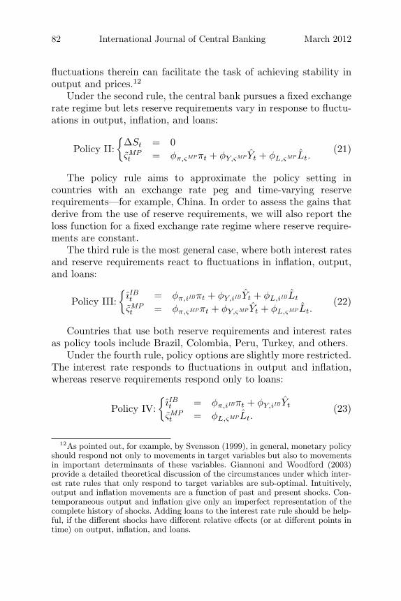
fluctuations therein can facilitate the task of achieving stability inoutput and prices.12
Under the second rule, the central bank pursues a fixed exchangerate regime but lets reserve requirements vary in response to fluctu-ations in output, inflation, and loans:
Policy II:{
ΔSt = 0ςMPt = φπ,ςMPπt + φY,ςMP Yt + φL,ςMPLt.
(21)
The policy rule aims to approximate the policy setting incountries with an exchange rate peg and time-varying reserverequirements—for example, China. In order to assess the gains thatderive from the use of reserve requirements, we will also report theloss function for a fixed exchange rate regime where reserve require-ments are constant.
The third rule is the most general case, where both interest ratesand reserve requirements react to fluctuations in inflation, output,and loans:
Policy III:{
ıIBt = φπ,iIBπt + φY,iIB Yt + φL,iIBLt
ςMPt = φπ,ςMPπt + φY,ςMP Yt + φL,ςMPLt.
(22)
Countries that use both reserve requirements and interest ratesas policy tools include Brazil, Colombia, Peru, Turkey, and others.
Under the fourth rule, policy options are slightly more restricted.The interest rate responds to fluctuations in output and inflation,whereas reserve requirements respond only to loans:
Policy IV:{
ıIBt = φπ,iIBπt + φY,iIB Yt
ςMPt = φL,ςMPLt.
(23)
12As pointed out, for example, by Svensson (1999), in general, monetary policyshould respond not only to movements in target variables but also to movementsin important determinants of these variables. Giannoni and Woodford (2003)provide a detailed theoretical discussion of the circumstances under which inter-est rate rules that only respond to target variables are sub-optimal. Intuitively,output and inflation movements are a function of past and present shocks. Con-temporaneous output and inflation give only an imperfect representation of thecomplete history of shocks. Adding loans to the interest rate rule should be help-ful, if the different shocks have different relative effects (or at different points intime) on output, inflation, and loans.
Vol. 8 No. 1 Reserve Requirements 83
We include policy IV in order to assess the costs of a separationof the monetary authority’s objectives. Since policy IV is a specialcase of policy III, the minimal loss under policy IV will be at leastas large as under policy III. In practice, however, assigning differ-ent targets to different instruments may improve accountability andfacilitate communication.
For each policy rule, the central bank then chooses the coeffi-cients that minimize the loss function under study. Tables 3 to 5(shown later in this paper when they are discussed individually)show the parameter values for the optimal policy projections (φ’s),which satisfy the following minimization problem:
φπ,x
φY,x
φL,x
⎫⎬⎭ = arg minφπ,x,φY,x,φL,x
LPS,FSt ∀x ∈ {iIB, ςMP}. (24)
The central bank also sets the rate at which reserves are remu-nerated. In our specification, we assume that the central bank keepsthe spread between the reserve rate and the interbank rate iIBt − iRtconstant. As can be seen from equation (5), such a policy impliesthat the difference between the actual reserve ratio and the targetratio ςMP
t − ςt remains constant.13
The government balances its budget every period. It uses theseignorage revenue net of interest payments to finance governmentexpenditure and lump-sum transfer payments. Government expendi-tures Gt follow an exogenous AR(1) process and lump-sum transfersTt adjust as a residual.
Gt − Tt = TSt
2.10 Shocks
Five shocks drive the economy’s dynamics: a cost-push shock (ξCPt ),
a technology shock (ξAt ), a government spending shock (Gt), a
foreign interest rate shock (i∗t ), and a foreign export demand shock
13If the central bank lets the spread vary, fluctuations in actual reserves becomea function of the parameter ψ2. The smaller ψ2 is, the more sensitive actualreserve holdings are to variations in the spread. A policy that keeps the spreadconstant therefore allows the central bank to control fluctuations in the reserverate directly, even if the cost for banks to deviate from the target ψ2 are relativelysmall.

84 International Journal of Central Banking March 2012
Table 1. Calibration of the Shocks
ρ σ2 Description
0.89 1.13 Technology Shock (ξAt )
0.40 0.14 Cost-Push Shock (ξCPt )
0.86 4.63 Government Expenditures Shock (Gt)0.88 0.43 Foreign Interest Rate Shock (i∗t )0.80 5.01 Export Demand Shock (Xt)
Notes: All shocks are defined as first-order stochastic difference equations, where ρ denotesthe degree of first-order autocorrelation and σ2 is the variance of the structural innovationof the shock processes.
Table 2. Calibration
Ident. Value Description
δ 0.025 Depreciation Rate of Capitalβ 0.985 Discount Factorα 0.33 Capital Share in Productionø 3.00 Inverse of Frish Labor Supply Elasticityθ 0.75 Degree of Price Stickinessυ 0.97 Survival Rate of Entrepreneursχ 0.25 Capital Adjustment Costsη 0.05 Elasticity of External Finance Premium to
Entrepreneurs’ Level of Leverage (fromthe Financial Accelerator; see appendix 1)
ψB 0.02 Adjustment Costs for Net Foreign Assetsγ 0.75 Share of Domestically Produced Goods in
Domestic Absorption
(Xt). All shocks follow AR(1) processes. The values attached to thevariance of the random shock component as well as the degree ofautocorrelation can be found in table 1. The values therein are takenfrom an estimated DSGE model as described in Christoffel, Coenen,and Warne (2008).
2.11 Calibration and Solution of the Model
Table 2 lists the details for parameters which are standard. Severalparameters are not calibrated directly and are specified such thatthey match model-specific variables to their empirical counterparts.

Vol. 8 No. 1 Reserve Requirements 85
This applies to the parameters ψ1 and the steady-state value ofςMPt in equation (2). These coefficients are calibrated such that they
imply an interest rate differential between the interbank rate (iIBt )and the interest rate on reserves (iRt ) in the steady state of 150 basispoints on quarterly basis and a steady-state share of reserve ratioof 0.10. The steady-state leverage ratio of entrepreneurs is two. Wechoose the other parameters of the financial contract to generate asteady-state external finance premium of 50 basis points and an elas-ticity to leverage of η = 0.05 (Christensen and Dib 2008). Combinedwith the interbank rate, this pins down the marginal steady-stateproductivity of capital and the ratio of output to capital. The impliedinvestment share is 0.22. We choose consumption share in output toequal 0.55, which implies a government share of 0.23. We assumethat 75 percent of total spending falls on home goods and balancedtrade in the long run. This implies that exports over output is 0.25.
Regarding the loss function, we choose for simplicity equalweights and set parameters λY and, where appropriate, λL equalto one.
In order to solve the model, we first log-linearize the non-linearequations system around the non-stochastic steady state. The log-linearized equilibrium equations are shown in appendix 2. In general,a hat denotes the percentage deviation from the steady state and atilde denotes level deviations.
3. Reserve Requirements as an Instrument for Price andFinancial Stability
Our analysis on the use of reserve requirements as a policy toolvaries along three dimensions. The first dimension is the financialstructure of the economy. We consider a first case where no financialfrictions are present, apart from the assumption that savings haveto be intermediated through banks and the requirement for banks tohold reserves. We then add a financial accelerator mechanism withdomestic currency debt in the second case and with foreign currencydebt in the third case.14 The second dimension is the central bank’sobjective. In the first example, the central bank has the relatively
14For the no-financial-accelerator case, we abstract from the role of entrepre-neurs, and capital is completely financed by deposits.
86 International Journal of Central Banking March 2012
standard objective of minimizing a weighted average of inflation andoutput variability; in the second example, the variability of loansenters additionally. The third dimension is operational: it includesthe number of variables the central bank monitors and how it usesits instruments.
The main aim of this section is therefore to analyze to whatextent the use of time-varying reserve requirements can improve pol-icy outcomes, as the structure of the economy, the objective of thecentral bank, and the implementation of policy varies. In section3.1 we analyze how the effects of discretionary changes in reserverequirements vary with other monetary arrangements and with thefinancial structure. The analysis of the transmission mechanism pre-pares the ground for the interpretation of the results in the subse-quent sections. Sections 3.2 and 3.3 present the results for the pricestability and financial stability objective function.
3.1 The Effects of Discretionary Changes in ReserveRequirements
The present section discusses how the effects of reserve requirementshocks change with monetary policy and the financial structure. Tosimplify the discussion, we assume that reserve requirements fol-low an exogenous AR(1) process with autocorrelation 0.7 and weabstract from a systematic component in reserve requirement policy.
We start by analyzing how the effects of changes in reserverequirements on the real economy depend on the use of other mon-etary policy instruments in an economy without a financial accel-erator. Changes in reserve requirements can have two effects: First,they influence the money supply. For a given monetary base, higherreserve requirements imply smaller broad money aggregates and weexpect an economic contraction. If the rate of reserve remunerationlies below the market interest rate, a second effect occurs: reserverequirements also act as a tax on the banking sector and drive awedge between deposit rates and lending rates. In the following wewill discuss the relative importance of the two effects under threedifferent monetary policies: a standard interest rate rule for the inter-bank rate as described by policy I in equation (20), a fixed exchangerate regime as given by policy II (see equation (21)), and, for illus-trative purposes, the textbook example of a monetary policy where

Vol. 8 No. 1 Reserve Requirements 87
base money supply is constant and there is no monetary policy rulefor the interbank rate (see, for instance, Burda and Wyplosz 2005).15
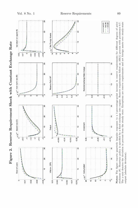
Figures 1, 2, and 3 show the effects of a 1-percentage-point dis-cretionary change of reserve requirements under different monetarypolicies for various degrees of price stickiness.
Under the interest rate rule, the effect as a tax on the bank-ing sector dominates. If the central bank targets an interest rate,money becomes endogenous and changes in reserve requirements areaccommodated. But higher reserve requirements increase the spreadbetween lending and deposit rates. Under the interest rate rule, thedeposit rate falls and the lending rate rises. A tightening throughan increase in reserve requirements leads therefore to quite differ-ent effects than a tightening through an increase in the policy rate,which would raise the level of interest rates in general. The higherspread has two important consequences. The increase in the lendingrate implies higher costs of credit for the real sector, which leadsto a decline in investment and the capital stock. The fall in invest-ment, however, does not necessarily lead to a decline in output, asthere is also an effect on consumption and on exports. A decline inthe deposit rate encourages consumption spending, as consumptionis linked to the real deposit rate through the Euler equation. Con-tractionary monetary policy would appreciate the exchange rate. Incontrast, an increase in reserve requirements tightens credit condi-tions and depreciates the exchange rate at the same time. Becauseof the uncovered interest parity, the decline in the deposit rate alsoleads to an exchange rate depreciation and a rise in exports. Becauseof the opposing effects on investment on the one side, and consump-tion and exports on the other side, the total effect on output isambiguous. For our calibration, inflation tends to increase, contraryto the popular notion that reserve requirements can be increased tocontain inflation. The increase in the tax on banks increases overallproduction costs, which puts upward pressures on the overall pricelevel.
The effects under a fixed exchange rate are broadly comparableto the ones under an interest rate rule, but with some notable dif-ferences. Under a fixed exchange rate and high capital mobility, the
15Base money (μt) is defined as total bank reserves: μtPt
= ςtDt. A constantbase money rule is characterized by Δμt = 0.

88 International Journal of Central Banking March 2012Fig
ure
1.R
eser
veR
equir
emen
tShock
with
anIn
tere
stR
ate
Rule
Note
s:T
he
figu
rere
por
tsqu
arte
rly
impuls
ere
spon
ses
toa
1-per
cent
age-
poi
ntin
crea
sein
rese
rve
requ
irem
ents
for
diff
eren
tdeg
rees
ofpri
cest
icki
nes
s(θ
).M
onet
ary
pol
icy
issp
ecifi
edby
anin
tere
stra
teru
lefo
rth
ein
terb
ank
inte
rest
rate
asdefi
ned
byeq
uat
ion
(20)
wit
hø π
,IB
=1.
5an
dot
her
coeffi
cien
tseq
ual
toze
ro.R
eser
vere
quir
emen
tsfo
llow
anA
R(1
)pro
cess
wit
hper
sist
ence
0.7.
The
y-ax
isden
otes
the
dev
iati
onin
per
cent
from
the
stea
dy
stat
e.E
xcep
tion
sar
ere
serv
ere
quir
emen
tsan
dnet
fore
ign
asse
tsov
erst
eady-
stat
eou
tput
(abso
lute
dev
iati
on).
An
incr
ease
inth
eex
chan
gera
teim
plies
adep
reci
atio
nof
the
dom
esti
ccu
rren
cy.
Vol. 8 No. 1 Reserve Requirements 89Fig
ure
2.R
eser
veR
equir
emen
tShock
with
Con
stan
tExch
ange
Rat
e
Note
s:T
he
figu
rere
por
tsqu
arte
rly
impuls
ere
spon
ses
toa
1-per
cent
age-
poi
ntin
crea
sein
rese
rve
requ
irem
ents
for
diff
eren
tdeg
rees
ofpri
cest
icki
nes
s(θ
).M
onet
ary
pol
icy
issp
ecifi
edby
afixe
dex
chan
gera
tere
gim
e.R
eser
vere
quir
emen
tsfo
llow
anA
R(1
)pro
cess
wit
hper
sist
ence
0.7.
The
y-ax
isden
otes
the
dev
iati
onin
per
cent
from
the
stea
dy
stat
e.E
xcep
tion
sar
ere
serv
ere
quir
emen
tsan
dnet
fore
ign
asse
tsov
erst
eady-
stat
eou
tput
(abso
lute
dev
iati
on).

90 International Journal of Central Banking March 2012Fig
ure
3.R
eser
veR
equir
emen
tShock
with
Con
stan
tB
ase
Mon
ey
Note
s:T
he
figu
rere
por
tsqu
arte
rly
impuls
ere
spon
ses
toa
1-per
cent
age-
poi
ntin
crea
sein
rese
rve
requ
irem
ents
for
diff
eren
tdeg
rees
ofpri
cest
icki
nes
s(θ
).M
onet
ary
pol
icy
issp
ecifi
edby
aco
nst
ant
bas
em
oney
rule
assp
ecifi
edin
the
text
.R
eser
vere
quir
emen
tsfo
llow
anA
R(1
)pro
cess
wit
hper
sist
ence
0.7.
The
y-ax
isden
otes
the
dev
iati
onin
per
cent
from
the
stea
dy
stat
e.E
xcep
tion
sar
ere
serv
ere
quir
emen
tsan
dnet
fore
ign
asse
tsov
erst
eady-
stat
eou
tput
(abso
lute
dev
iati
on).
An
incr
ease
inth
eex
chan
gera
teim
plies
adep
reci
atio
nof
the
dom
esti
ccu
rren
cy.

Vol. 8 No. 1 Reserve Requirements 91
central bank is forced to stabilize the nominal deposit rate almostcompletely and the increase is absorbed by the lending rate. Theincrease in consumption, stemming from a decrease in ex ante realinterest rates, is more muted and the effect on investment prevails.
Under a constant base money rule, the impulse responses arequalitatively similar to those of a standard contractionary mone-tary policy interest rate shock. Interest rates rise, whereas outputand inflation fall. The increase in reserve requirements increases thedemand for deposits by banks. In order to attract more deposits,the deposit rate has to increase. This puts upward pressure on lend-ing rates, as marginal funding costs increase. As in the other cases,investment declines, but now, due to the rise in the deposit rate,consumption declines as well. This leads to an unambiguous declinein prices and output. Compared with the other policies considered,the magnitude of the responses is substantially larger; for example,the decline in investment is about ten times larger. The effect thatderives from the contraction in broad money dominates the effectsfrom the tax on banks.16 However, the money multiplier effect isonly important if there are nominal rigidities. The impulse responsefunctions in figures 1, 2, and 3 show each variable’s reaction for dif-ferent degrees of price stickiness. Under the constant base moneypolicy, the effects of reserve requirements are more sensitive to pricestickiness than under the other two monetary policies. Without pricestickiness, the reaction of the real variables is the same independentof the underlying monetary policy. This can be seen well in figures1 and 2 by means of the black solid line. In the case of figure 3, thereal variables show exactly the same reaction as in figures 1 and 2;however, due to the scaling of the y-axis, this can be hardly distin-guished from zero. Intuitively, monetary effects overturn the effectsfrom the tax only if nominal rigidities are important.
We now turn to a discussion on the effects of including a financialaccelerator mechanism. Figure 4 compares the effects of a reserverequirement shock with no financial accelerator, with a financial
16The different magnitudes under alternative monetary regimes also help toexplain the fact that authorities in Brazil and Croatia cut reserve requirementsby 10 percentage points and more in the recent financial crisis, while textbookdescriptions that treat reserve requirements from a constant base money perspec-tive warn of the potentially large effects that derive from small changes in reserverequirements (see, for instance, Burda and Wyplosz 2005, p. 206).

92 International Journal of Central Banking March 2012Fig
ure
4.R
eser
veR
equir
emen
tShock
and
Fin
anci
alFri
ctio
ns
Note
s:T
he
figu
rere
por
tsqu
arte
rly
impuls
ere
spon
ses
toa
1-per
cent
age-
poi
ntin
crea
sein
rese
rve
requ
irem
ents
.M
onet
ary
pol
icy
issp
ecifi
edby
anin
tere
stra
teru
lefo
rth
ein
terb
ank
inte
rest
rate
asdefi
ned
byeq
uat
ion
(20)
wit
hø π
,IB
=1.
5an
dot
her
coeffi
cien
tseq
ual
toze
ro.
Res
erve
requ
irem
ents
follow
anA
R(1
)pro
cess
wit
hper
sist
ence
0.7.
The
adju
stm
ent
ofth
eec
onom
yis
show
nfo
rdiff
eren
tm
odel
spec
ifica
tion
s;in
par
ticu
-la
r,th
esc
enar
ios
repre
sent
(i)
am
odel
wit
hth
efinan
cial
acce
lera
tor
bas
edon
dom
esti
ccu
rren
cydeb
t,(i
i)a
mod
elw
ith
the
finan
cial
acce
lera
tor
bas
edon
fore
ign
curr
ency
deb
t,an
d(i
ii)
am
odel
wit
hou
tth
efinan
cial
acce
lera
tor.
The
y-ax
isden
otes
the
dev
iati
onin
per
cent
from
the
stea
dy
stat
e.E
xcep
tion
sar
ere
serv
ere
quir
emen
tsan
dnet
fore
ign
asse
tsov
erst
eady-
stat
eou
tput
(abso
lute
dev
iati
on).
An
incr
ease
inth
eex
chan
gera
teim
plies
adep
reci
atio
nof
the
dom
esti
ccu
rren
cy.

Vol. 8 No. 1 Reserve Requirements 93
accelerator and domestic currency debt, and with a financial mecha-nism and foreign currency debt under an interest rate policy. In com-parison with the baseline case, introducing a financial acceleratorwith domestic currency debt strengthens the effect on investment.Because of movements in the external finance premium, investmentbecomes more sensitive to fluctuations in the interbank rate. For-eign currency debt amplifies the transmission of reserve require-ment shocks on investment further. The fall in investment is aboutfour times larger than in the case without a financial accelerator.The decline in the deposit rate depreciates the domestic currency,which increases the domestic currency value of firms’ debt, net worthdeclines, and the external finance premium rises further. Foreigncurrency debt strengthens therefore the transmission mechanism ofreserve requirements—in particular, if the central bank follows aninterest rate rule. This is in contrast to policy interest rate increases,where the contractionary effects of interest hikes tend to be weakenedbecause of a currency appreciation and an increase in entrepreneurs’net worth.
3.2 Optimal Reserve Requirement Rules with a Price StabilityObjective
In the present section we keep the objective fixed and consider onlythe price stability loss function defined in equation (18), while wevary the structure of the economy and the operational policy rules.
We start with a situation where the central bank only moni-tors fluctuations in output and inflation and does not respond toloans (labeled setting A). The results are displayed in table 3. Wereport the optimized coefficients in the policy rules and the valueof the resulting loss function—in particular, its absolute value andthe value relative to a policy that keeps the exchange rate and thereserve requirement ratio (ςMP
t ) constant.Consider first the economy without financial frictions. The main
result is that the use of reserve requirements adds little in termsof economic stabilization. Under policy A(III), where the centralbank sets reserve requirements in addition to interest rates, the lossfunction is only about 2 percent lower compared with policy A(I),where the reserve requirement ratio is kept constant throughout.By comparison, the corresponding loss function value for the United

94 International Journal of Central Banking March 2012
Table 3. Optimal Policy Rules under a PriceStability Objective
Policy A(I) Policy A(II) Policy A(III)
iIBt ςMPt iIBt ςMP
t iIBt ςMPt
Without Financial Frictions
øY,j 0.2 — — 10.8 0.1 5.9øπ,j 2.1 — — 28.6 1.9 12.5
LPS 17.2 (0.42) 40.2 (0.98) 16.8 (0.41)
With Financial Frictions and Domestic Currency Debt
øY,j 0.6 — — 13.2 0.4 11.0øπ,j 2.8 — — 31.9 2.2 17.5
LPS 23.1 (0.48) 45.3 (0.94) 20.7 (0.43)
With Financial Frictions and Foreign Currency Debt
øY,j 0.7 — — 13.2 0.5 15.3øπ,j 3.1 — — 31.9 2.9 28.9
LPS 26.1 (0.54) 45.3 (0.94) 23.7 (0.49)
Notes: The table shows the parameter values for policy A(I), policy A(II), and policyA(III) as specified in equations (20)–(22) for the optimal policy projections under the lossfunction defined in equation (18). The value in parentheses denotes the value relative tofixed exchange rate policy with constant reserve requirements.
States from 1960:Q1 to 1983:Q4 is about 4.3 times higher than from1984:Q1 to 2007:Q2.17 Under a fixed exchange rate regime, the valueof the loss function is more than twice as large as under an interestrate rule (reported in parentheses) and the gains from using reserverequirements under an exchange rate peg are limited. The loss func-tion is only about 2 percent smaller. Adding financial frictions doesnot alter the general picture. Not surprisingly, the absolute valueof the loss function is higher in each case. In addition, the optimal
17Our inflation measure is quarter-to-quarter CPI inflation; output gap andcredit gap are the percentage deviation from trend computed with a Hodrick-Prescott filter with smoothing parameter 1,600. Data for real GDP and CPI arefrom the Federal Reserve Bank of St. Louis database; credit is from the IMFInternational Financial Statistics (line 22d).

Vol. 8 No. 1 Reserve Requirements 95
response to output and inflation fluctuations is generally stronger.While we obtain the same ranking of the policy rules, the relativegains of policy A(III) over policy A(I) are slightly larger, improvingby about 10 percent with domestic currency debt and with foreigncurrency debt. Foreign currency debt weakens also the advantage ofinterest rate rules over exchange rate pegs, as foreign currency debtweakens the effects of interest rate movements on output because ofbalance sheet effects.18
We turn now to situation B, where the central bank also respondsto fluctuations in loans but minimizes the same loss function (LPS
t )as before. Note that here the central bank responds to loans becausethey contain information about the state of the economy, not becausethe containment of loan fluctuations is an end in itself. The resultsare reported in table 4. In an economy without financial frictions,the use of reserve requirements brings again little gain, both underan interest rate rule and under a peg. Losses are between 3 and4 percent smaller. However, reacting to loans leads to lower losses.Compared with setting A, losses are about 10 percent smaller. Theresult indicates that even in an economy without financial frictions,responding to loans can generate some benefits, as loans containuseful information about the state of the economy.19
Introducing a financial accelerator mechanism with domestic cur-rency debt leads to two new important results. First, using reserverequirements as a second policy tool helps to stabilize the econ-omy. The loss function under policy B(III) is 22 percent lower thanunder policy B(I). Second, separating the targets for interest ratesand reserve requirements leads to only minor losses in terms of eco-nomic stabilization. Under policy B(IV), where reserve requirementsrespond only to loans and interest rates to output and inflation, theloss function is only 3 percent higher than under the more general
18Results for the reserve requirement rule under a peg are unaffected by foreigncurrency debt, as the exchange rate is constant.
19A shock-specific analysis (using the previously optimized policy rules) indi-cates that the gains derive mainly from lower loss functions for technology, cost-push, and external demand shocks. For standard calibrations, these shocks inducemore relative variation in loans than foreign interest rate and goverment spendingshocks. A larger degree of variation in turn may increase the predictive contentfor inflation and output.
96 International Journal of Central Banking March 2012
Table 4. Optimal Policy Rules under a PriceStability Objective
Policy B(I) Policy B(II) Policy B(III) Policy B(IV)
iIBt ςMPt iIBt ςMP
t iIBt ςMPt iIBt ςMP
t
Without Financial Frictions
øL,j 0.7 — — 13.3 0.2 5.5 — 13.6øY,j 0.3 — — 8.5 0.1 7.1 0.2 —øπ,j 2.4 — — 35.6 2.1 16.7 2.5 —
LPS 15.6 (0.38) 39.4 (0.96) 15.2 (0.37) 15.5 (0.38)
With Financial Frictions and Domestic Currency Debt
øL,j 0.9 — — 18.7 0.7 15.7 — 19.7øY,j 0.4 — — 10.0 0.3 6.1 0.2 —øπ,j 2.8 — — 39.9 2.7 21.6 2.5 —
LPS 19.8 (0.41) 43.3 (0.91) 15.4 (0.32) 15.9 (0.33)
With Financial Frictions and Foreign Currency Debt
øL,j 1.3 — — 18.7 0.8 23.0 — 25.4øY,j 0.5 — — 10.0 0.4 10.9 0.2 —øπ,j 3.3 — — 39.9 2.4 19.1 2.5 —
LPS 23.2 (0.48) 43.3 (0.91) 16.9 (0.35) 17.0 (0.35)
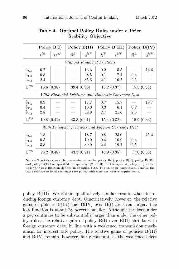
Notes: The table shows the parameter values for policy B(I), policy B(II), policy B(III),and policy B(IV) as specified in equations (20)–(23) for the optimal policy projectionsunder the loss function defined in equation (18). The value in parentheses denotes thevalue relative to fixed exchange rate policy with constant reserve requirements.
policy B(III). We obtain qualitatively similar results when intro-ducing foreign currency debt. Quantitatively, however, the relativegains of policies B(III) and B(IV) over B(I) are even larger: Theloss function is about 28 percent smaller. Although the loss undera peg continues to be substantially larger than under the other pol-icy rules, the relative gain of policy B(I) over B(II) shrinks withforeign currency debt, in line with a weakened transmission mech-anism for interest rate policy. The relative gains of policies B(III)and B(IV) remain, however, fairly constant, as the weakened effect

Vol. 8 No. 1 Reserve Requirements 97
of interest rate changes is compensated by stronger effects of reserverequirements.
3.3 Optimal Reserve Requirement Rules with a FinancialStability Objective
In this section we consider a case where the central bank explicitlywants to stabilize the fluctuations in loans, as reflected in the lossfunction LFS
t in equation (19).The results are displayed in table 5. The optimal policy rules
imply four key results: First, the use of reserve requirements as apolicy tool leads to substantially lower loss function values, but onlyif there are financial frictions. Compared with policy C(III), the lossunder policy C(I) rises by around 53 percent with domestic cur-rency debt and by even more (89 percent) in the economy withforeign currency debt. For the foreign currency debt, the percentagereduction in the loss function corresponds to roughly 30 percent ofthe percentage reduction the United States has experienced in thecorresponding loss function in the Great Moderation period.20 Thehigher loss under policy C(I) can be explained with the example ofa technology shock as depicted in figure 5. The expansionary shocktriggers a decline in inflation and an increase in loans. A policyaiming to stabilize inflation would favor a decline in the interbankinterest rate in order to keep real rates low. The macroprudentialpolicy, however, would favor an increase in the interbank rate whichthen attenuates credit demand of entrepreneurs. Hence, two goalsshould be implemented with one policy instrument: the interbankrate should increase and decrease at the same time. The final reac-tion of the interest rate will be such that it accommodates bothpolicy goals imperfectly.
Second, a separation of tasks, where reserve requirements onlyrespond to loans and interest rates to output and inflation fluctua-tions leads only to minor stabilization losses. Under policy C(III),both interest rates and reserve requirements react simultaneouslyto developments in output, inflation, and loans. Such a framework
20From 1960:Q1 to 1983:Q4 the loss function value is about 310 percent largerthan from 1984:Q1 to 2007:Q2.

98 International Journal of Central Banking March 2012
Table 5. Optimal Policy Rules with a FinancialStability Objective
Policy C(I) Policy C(II) Policy C(III) Policy C(IV)
iIBt ςMPt iIBt ςMP
t iIBt ςMPt iIBt ςMP
t
Without Financial Frictions
øL,j 0.9 — — 21.8 0.6 13.7 — 9.2øY,j 0.1 — — 9.3 0.1 5.7 0.4 —øπ,j 3.1 — — 28.9 2.6 21.1 3.4 —
LFS 24.5 (0.52) 46.2 (0.98) 21.7 (0.46) 22.6 (0.48)
LPS|FS/L
PS 1.39 1.06 1.25 1.26
With Financial Frictions and Domestic Currency Debt
øL,j 1.2 — — 31.2 0.8 26.1 — 13.9øY,j 0.1 — — 13.5 0.1 7.3 0.3 —øπ,j 3.6 — — 27.2 2.8 16.4 3.3 —
LFS 33.7 (0.57) 53.8 (0.91) 22.1 (0.37) 22.9 (0.37)
LPS|FS/L
PS 1.50 1.17 1.24 1.22
With Financial Frictions and Foreign Currency Debt
øL,j 1.2 — — 31.2 1.1 25.1 — 20.7øY,j 0.2 — — 13.5 0.1 8.9 0.4 —øπ,j 3.9 — — 27.2 2.9 13.4 3.4 —
LFS 40.2 (0.68) 53.8 (0.91) 21.2 (0.35) 21.4 (0.36)
LPS|FS/L
PS 1.65 1.17 1.05 1.06
Notes: The table shows the parameter values for policy C(I), policy C(II), policy C(III),and policy C(IV) as specified in equations (20)–(23) for the optimal policy projectionsunder the loss function defined in equation (19). The value in parentheses denotes thevalue relative to fixed exchange rate policy with constant reserve requirements.
might not be very transparent and therefore difficult to commu-nicate. Under policy C(IV), reserve requirements only respond tofluctuations in loans, whereas interest rates focus on output andinflation. As can be seen from table 5, policy C(IV) implies nearlythe same loss function as policy C(III). As discussed in section 3.1, areserve requirement increase unambiguously lowers aggregate credit

Vol. 8 No. 1 Reserve Requirements 99Fig
ure
5.Tec
hnol
ogy
Shock
Note
s:T
he
figu
rere
por
tsqu
arte
rly
impuls
ere
spon
ses
toan
expan
sion
ary
tech
nol
ogy
shoc
k.M
onet
ary
pol
icy
issp
ecifi
edby
the
thre
epol
icy
regi
mes
outl
ined
inse
ctio
n3.
2th
atm
inim
ize
loss
funct
ion
(24)
asre
por
ted
inta
ble
3.T
her
eis
no
finan
cial
acce
lera
tor.
The
y-ax
isden
otes
the
dev
iati
onin
per
cent
from
the
stea
dy
stat
e.E
xcep
tion
sar
ere
serv
ere
quir
emen
tsan
dnet
fore
ign
asse
tsov
erst
eady-
stat
eou
tput
(abso
lute
dev
iati
on).
An
incr
ease
inth
eex
chan
gera
teim
plies
adep
reci
atio
nof
the
dom
esti
ccu
rren
cy.
100 International Journal of Central Banking March 2012
but tends to have small and ambiguous effects on inflation and out-put. Since reserve requirement policy has small direct effects on out-put and inflation, a reserve requirement rule that focuses on loansleads only to small losses.
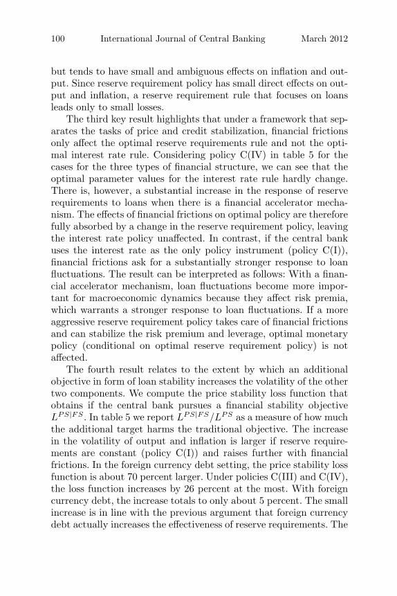
The third key result highlights that under a framework that sep-arates the tasks of price and credit stabilization, financial frictionsonly affect the optimal reserve requirements rule and not the opti-mal interest rate rule. Considering policy C(IV) in table 5 for thecases for the three types of financial structure, we can see that theoptimal parameter values for the interest rate rule hardly change.There is, however, a substantial increase in the response of reserverequirements to loans when there is a financial accelerator mecha-nism. The effects of financial frictions on optimal policy are thereforefully absorbed by a change in the reserve requirement policy, leavingthe interest rate policy unaffected. In contrast, if the central bankuses the interest rate as the only policy instrument (policy C(I)),financial frictions ask for a substantially stronger response to loanfluctuations. The result can be interpreted as follows: With a finan-cial accelerator mechanism, loan fluctuations become more impor-tant for macroeconomic dynamics because they affect risk premia,which warrants a stronger response to loan fluctuations. If a moreaggressive reserve requirement policy takes care of financial frictionsand can stabilize the risk premium and leverage, optimal monetarypolicy (conditional on optimal reserve requirement policy) is notaffected.
The fourth result relates to the extent by which an additionalobjective in form of loan stability increases the volatility of the othertwo components. We compute the price stability loss function thatobtains if the central bank pursues a financial stability objectiveLPS|FS. In table 5 we report LPS|FS/LPS as a measure of how muchthe additional target harms the traditional objective. The increasein the volatility of output and inflation is larger if reserve require-ments are constant (policy C(I)) and raises further with financialfrictions. In the foreign currency debt setting, the price stability lossfunction is about 70 percent larger. Under policies C(III) and C(IV),the loss function increases by 26 percent at the most. With foreigncurrency debt, the increase totals to only about 5 percent. The smallincrease is in line with the previous argument that foreign currencydebt actually increases the effectiveness of reserve requirements. The

Vol. 8 No. 1 Reserve Requirements 101
Table 6. Optimal Policy Rules with ImperfectCapital Mobility
No FA FA with DCD FA with FCD
C(I) C(IV) C(I) C(IV) C(I) C(IV)
Low Capital Mobility 28.8 26.4 38.6 34.5 49.9 33.1High Capital Mobility 24.5 22.6 33.7 22.9 40.2 21.4
(compare Table 5)
Notes: The table shows the value of the loss function defined in equation (19) under highand low capital mobility (ψB = 0.02 and ψB = 0.10). The policy rules correspond to thoseoutlined in table 5. “No FA” refers to the model without the financial accelerator, “FAwith DCD” features the financial accelerator based on domestic currency debt, and “FAwith FCD” features it based on foreign currency debt.
result indicates that asking the central bank to control credit canlead to substantially higher fluctuations in output and prices withoutan additional instrument, but that the use of reserve requirementscan contain the resulting losses.
4. Extensions: Limited Capital Mobility and the Role ofSpecific Shocks
The present section considers two extensions. First, we consider howlimited capital mobility affects our results. Second, we analyze therole of specific shocks. In both cases the central bank has a finan-cial stability loss function. To save space, we focus on the policieswhere only the interest rate moves, C(I), and reserve requirementsand interest rates pursue separate tasks, C(IV).
In many emerging countries capital mobility is imperfect, bothbecause of technical impediments and because of capital controls.Capital controls are sometimes under discussion as a substitutefor macroprudential policies. To analyze the role of limited capi-tal mobility, we increase the sensitivity of the country risk premiumψB from 0.02 to 0.10. The increased sensitivity makes the financingof external imbalances more costly and moves the economy towardsfinancial autarky.21 Table 6 compares the results for low and high
21In the present analysis costs are symmetric for in- and outflows. Consideringasymmetries could be an interesting extension.

102 International Journal of Central Banking March 2012
Table 7. Optimal Policy Rules for Specific Shocks
No FA FA with DCD FA with FCD
C(I) C(IV) C(I) C(IV) C(I) C(IV)
Technology 1.00 0.96 1.54 1.01 1.94 1.22Cost Push 1.00 0.92 1.38 1.07 2.07 1.46Government Expenditures 1.00 0.91 1.05 1.02 1.37 1.18Foreign Interest Rate 1.00 0.99 1.33 1.26 1.53 1.38Export Demand 1.00 0.99 1.10 1.07 1.17 1.13
Notes: The table shows the value of the loss function defined in equation (19) if onlyone type of shock hits the economy. The policy rules considered for the interest rate andreserve requirements correspond to those outlined in table 5. “No FA” refers to the modelwithout the financial accelerator, “FA with DCD” features the financial accelerator basedon domestic currency debt, and “FA with FCD” features it based on foreign currency debt.
capital mobility. There are two main findings: First, capital con-trols increase the loss function values for both type of policy rules,irrespective of the financial structure. Imperfect capital mobility con-strains the possibility of the economy to absorb shocks through thecurrent account. Second, capital controls reduce the effectiveness ofreserve requirements. The loss of policy C(I) relative to C(IV) dropsfrom 1.5 to 1.1 with domestic currency debt and from 1.9 to 1.5 withforeign currency debt. Limited capital mobility increases the offset-ting effects of reserve requirements on consumption, as consumptionsmoothing possibilities are limited. Furthermore, in the foreign cur-rency debt case, the effects of reserve requirement changes becomesmaller, as the nominal exchange rate response becomes more muted.
We intend to analyze to what extent our results are affected bythe types of shocks that hit the economy. Table 7 considers eachof the five shocks separately when the central bank has a financialstability objective (LFS). Different from the previous exercise, thecentral bank chooses different coefficients for each type of shock.While such a setting is admittedly unrealistic, it allows us to assesswhether our results are driven by a specific shock and if the hetero-geneity in the optimal responses conditional on some specific shockis important.
The results broadly confirm our previous findings but highlightthat the results for specific shocks vary with the financial structureof the economy. If there is no financial accelerator mechanism, the

Vol. 8 No. 1 Reserve Requirements 103
gains of using reserve requirements are limited for all types ofshocks, in line with our previous finding. In the model with a finan-cial accelerator and domestic currency debt, the gains from usingreserve requirements derive mainly from supply shocks (cost pushand technology), whereas they remain small for demand and foreignshocks. A financial accelerator mechanism amplifies both the effectsof reserve requirements and of policy rate changes. A reserve require-ment rule that responds to loan fluctuations generates substantialbenefits only for those shocks that do not move loans, output, andinflation in the same direction. For other shocks, interest rate policycan move all target variables in the desired direction. With foreigncurrency debt, there are also gains for demand and foreign shockswhen applying a reserve requirement rule. Foreign currency debtcomplicates the task of interest rate policy to stabilize loans forall shocks. While a raise in the policy rate increases risk-free rates,the associated exchange rate appreciation increases entrepreneurs’net worth, which leads to a decline in risk premia and attenuatesthe contraction in loans. At the same time, foreign currency debtincreases the effects of discretionary reserve requirement changes.
5. Conclusion
The present paper aims to provide a framework to analyze if andunder which circumstances reserve requirements can be an effectivetool. We build a small open-economy model with nominal rigidities,financial frictions, and a banking sector that is subject to reserverequirements. If the central bank pursues mainly a price stabilityobjective and uses the interest rate as its main policy instrument,varying reserve requirements contributes little to economic stability.Higher reserve requirements increase interest rate spreads, whichinduces upward pressure on consumption due to lower deposit rates,and downward pressure on investment due to higher lending rates.However, if there are financial frictions—in particular, in conjunctionwith foreign currency debt and an objective to stabilize credit—thegains from adapting reserve requirements to economic conditions aresubstantial. An increase in reserve requirements allows to generatean exchange rate depreciation and tougher credit conditions at thesame time, whereas interest rate policy through interest rates has toforgive one or the other.

104 International Journal of Central Banking March 2012
We interpret our results as reflecting the Tinbergen rule. Asnoted by Tinbergen (1952), the policymaker cannot intend to hittargets for more objective variables than the number of instrumentsavailable. However, as Tinbergen (1952) emphasizes, the availabilityof N instruments does not guarantee that as many as N objectivetargets can be hit. There must be N independent instruments, in thesense that the effects of any one instrument on the objectives are notproportional to those of any other, or of any combination of others.In line with this, we find that in an economy without financial fric-tions and where the central bank pursues a price stability mandate,the gains from using reserve requirements as an additional instru-ment are negligible but can improve policy outcomes substantiallyin an economy where financial frictions are present and the centralbank has a financial stability objective.
Appendix 1. Financial Contract between Lending Banksand Entrepreneurs
This appendix refers to section 2.5. The loan contract between entre-preneurs and lending bank units introduces a further friction into themodel. This contract’s structure is as described in Bernanke, Gertler,and Gilchrist (1999). The financial contract involves two parties:an entrepreneur with net worth and a bank which can raise fundsfrom households. There is a continuum of entrepreneurs indexed byj ∈ (0, 1) who purchase a capital stock from capital goods produc-ers and rent it to intermediate goods producers. Each entrepreneurfinances his end-of-time-t capital holdings with his end-of-time-t networth and bank loans from the financial intermediary. Let Nt(j) behis net worth, Lt(j) his stock of loans, Qt the current market priceof one unit of capital and Kt(j) its end-of-time-t capital stock, andthen this entrepreneur’s balance sheet reads
QtKt(j) = Nt(j) + Lt(j). (25)
Capital is homogeneous and so it does not matter whether capitalpurchased by the entrepreneur is newly produced within the currentperiod or is old, already depreciated, capital. Having the entrepre-neur purchase his total capital stock each period makes sure that
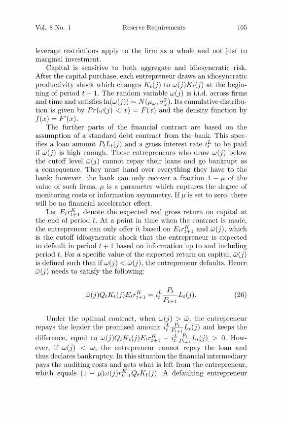
Vol. 8 No. 1 Reserve Requirements 105
leverage restrictions apply to the firm as a whole and not just tomarginal investment.
Capital is sensitive to both aggregate and idiosyncratic risk.After the capital purchase, each entrepreneur draws an idiosyncraticproductivity shock which changes Kt(j) to ω(j)Kt(j) at the begin-ning of period t + 1. The random variable ω(j) is i.i.d. across firmsand time and satisfies ln(ω(j)) ∼ N(μω, σ2
ω). Its cumulative distribu-tion is given by Pr(ω(j) < x) = F (x) and the density function byf(x) = F ′(x).
The further parts of the financial contract are based on theassumption of a standard debt contract from the bank. This spec-ifies a loan amount PtLt(j) and a gross interest rate iLt to be paidif ω(j) is high enough. Those entrepreneurs who draw ω(j) belowthe cutoff level ω(j) cannot repay their loans and go bankrupt asa consequence. They must hand over everything they have to thebank; however, the bank can only recover a fraction 1 − μ of thevalue of such firms. μ is a parameter which captures the degree ofmonitoring costs or information asymmetry. If μ is set to zero, therewill be no financial accelerator effect.
Let EtrKt+1 denote the expected real gross return on capital at
the end of period t. At a point in time when the contract is made,the entrepreneur can only offer it based on Etr
Kt+1 and ω(j), which
is the cutoff idiosyncratic shock that the entrepreneur is expectedto default in period t + 1 based on information up to and includingperiod t. For a specific value of the expected return on capital, ω(j)is defined such that if ω(j) < ω(j), the entrepreneur defaults. Henceω(j) needs to satisfy the following:
ω(j)QtKt(j)EtrKt+1 = iLt
Pt
Pt+1Lt(j). (26)
Under the optimal contract, when ω(j) > ω, the entrepreneurrepays the lender the promised amount iLt
Pt
Pt+1Lt(j) and keeps the
difference, equal to ω(j)QtKt(j)EtrKt+1 − iLt
Pt
Pt+1Lt(j) > 0. How-
ever, if ω(j) < ω, the entrepreneur cannot repay the loan andthus declares bankruptcy. In this situation the financial intermediarypays the auditing costs and gets what is left from the entrepreneur,which equals (1 − μ)ω(j)rK
t+1QtKt(j). A defaulting entrepreneur
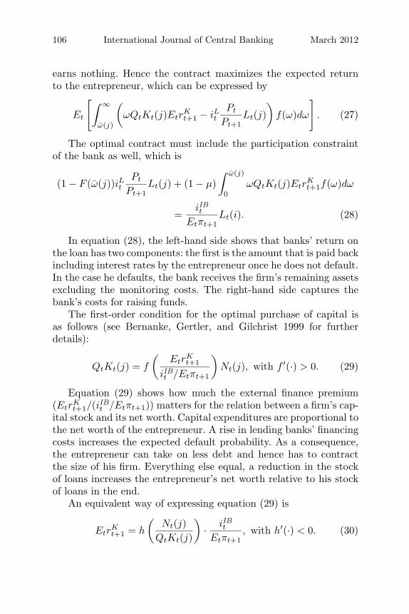
106 International Journal of Central Banking March 2012
earns nothing. Hence the contract maximizes the expected returnto the entrepreneur, which can be expressed by
Et
[∫ ∞
ω(j)
(ωQtKt(j)Etr
Kt+1 − iLt
Pt
Pt+1Lt(j)
)f(ω)dω
]. (27)
The optimal contract must include the participation constraintof the bank as well, which is
(1 − F (ω(j))iLtPt
Pt+1Lt(j) + (1 − μ)
∫ ω(j)
0ωQtKt(j)Etr
Kt+1f(ω)dω
=iIBt
Etπt+1Lt(i). (28)
In equation (28), the left-hand side shows that banks’ return onthe loan has two components: the first is the amount that is paid backincluding interest rates by the entrepreneur once he does not default.In the case he defaults, the bank receives the firm’s remaining assetsexcluding the monitoring costs. The right-hand side captures thebank’s costs for raising funds.
The first-order condition for the optimal purchase of capital isas follows (see Bernanke, Gertler, and Gilchrist 1999 for furtherdetails):
QtKt(j) = f
(Etr
Kt+1
iIBt /Etπt+1
)Nt(j), with f ′(·) > 0. (29)
Equation (29) shows how much the external finance premium(Etr
Kt+1/(iIBt /Etπt+1)) matters for the relation between a firm’s cap-
ital stock and its net worth. Capital expenditures are proportional tothe net worth of the entrepreneur. A rise in lending banks’ financingcosts increases the expected default probability. As a consequence,the entrepreneur can take on less debt and hence has to contractthe size of his firm. Everything else equal, a reduction in the stockof loans increases the entrepreneur’s net worth relative to his stockof loans in the end.
An equivalent way of expressing equation (29) is
EtrKt+1 = h
(Nt(j)
QtKt(j)
)· iIBtEtπt+1
, with h′(·) < 0. (30)

Vol. 8 No. 1 Reserve Requirements 107
For an entrepreneur who is not fully self-financed, the expectedreturn to capital has to be equal to the marginal cost of externalfinance. Equation (30) expresses the equilibrium condition that theratio rK
t+1/(iIBt /Etπt+1) of the cost of external finance to the safe ratedepends on the share of the entrepreneur’s new capital purchase thatis financed by his own net worth.
Appendix 2. The Log-Linearized Equations
The following equations describe the equilibrium of the model inlog-linearized form as referred to in section 2.11. The equationshere refer to the model with domestic currency debt. A hat denotesthe percentage deviation from the steady state and a tilde denoteslevel deviations. The variable Bt denotes the deviation of net foreignassets from the steady-state level of output.
Households
• Consumption-saving decision:
EtCt+1 − Ct = ıDt − Etπt+1
• Uncovered interest parity condition:
ıDt + ψBBt = ı∗t + EtΔst+1
• Labor supply:
wt = φht + Ct
Deposit Banks
• Reserve requirements:
ıIBt =iR
iIBıRt − ψ2
(ςt − ςMP
t
)• Deposit rate:
ıDt = a1ıIBt − a2ς
MPt ,
where a1 = (1 − ς) iIB
iD + ς iR
iD and a2 = iIB−iR
iD .

108 International Journal of Central Banking March 2012
Entrepreneurs and Lending Banks
• Leverage and external finance premium:
EtrKt+1 − ıIBt + Etπt+1 = η[Qt + Kt − Nt]
• Loan rate (nominal and real):
rLt = Qt + Kt + Etr
Kt+1 − Lt
ıLt = rLt + Etπt+1
Entrepreneurs
• Balance sheet:
Qt + Kt = εLLt + (1 − εL)Nt
• Net worth:
Nt = νNt−1 + (1 − ν)[Qt−1 + Kt−1] + rKt
+ νεL
1 − εL
[rKt −
(ıLt−1 − πt
)]Intermediate Goods Producers
• Production function:
yt = ξAt + αKt−1 + (1 − α)ht
• Marginal costs:
mct = αzt + (1 − α)Wt − ξAt
• Cost minimization:
ht + Wt = zt + Kt−1
• Price setting:
πdt = βEtπ
dt+1 +
(1 − θ)(1 − θβ)θ
mct + ξCPt

Vol. 8 No. 1 Reserve Requirements 109
Capital Goods Producers
• Investment demand:
Qt = χ[It − Kt−1]
• Price of capital:
rKt − Qt−1 =
MPKrK
zt +1 − δ
rKQt,
where MPK is the marginal product of capital.
• Capital dynamics:
Kt = (1 − δ)Kt−1 + δIt
Monetary and Macroprudential Policy
See section 2.9 and section 3.2 for the details.
Market Clearing
• Goods market:
Yt = γ[cyCt + iy It + gyGt + (1 − γ)εt] + (1 − γ)[εt + Xt]
• Balance of payments:
Bt = Yt − [cyCt + iy It + gyGt + (1 − γ)εt] + i∗Bt−1
• Real exchange rate:
εt − εt−1 = Δst − πdt
• CPI—inflation rate:
πt = γπdt + (1 − γ)Δst
References
Baltensperger, E. 1982. “Reserve Requirements and Economic Sta-bility.” Journal of Money, Credit, and Banking 14 (2): 205–15.

110 International Journal of Central Banking March 2012
Basci, E. 2010. “Central Banks and Financial Stability.” Presenta-tion at the ECB High-Level Policy Workshop on MacroprudentialPolicy, Frankfurt, December 15.
Bean, C., M. Paustian, A. Penalver, and T. Taylor. 2010. “MonetaryPolicy after theFall.”Paper presented at theFederalReserveBankof Kansas City Economic Symposium on Macroeconomic Chal-lenges: The Decade Ahead, Jackson Hole, Wyoming, August 28.
Bernanke, B., M. Gertler, and S. Gilchrist. 1999. “The FinancialAccelerator in a Quantitative Business Cycle Framework.” InHandbook of Macroeconomics, Vol. 1C, ed. J. B. Taylor and M.Woodford (chapter 21). Amsterdam: North-Holland.
Blanchard, O. 2009. “The State of Macro.” Annual Review of Eco-nomics 1 (1): 209–28.
Bokan, N., L. Grguric, I. Krznar, and M. Lang. 2009. “The Impact ofthe Financial Crisis and Policy Responses in Croatia.” CroatianNational Bank Working Paper No. 22 (December).
Borio, C., and M. Drehmann. 2009. “Assessing the Risk of BankingCrises—Revisited.” BIS Quarterly Review (March): 29–46.
Borio, C., and P. Lowe. 2002. “Assessing the Risk of Banking Crises.”BIS Quarterly Review (December): 43–54.
Burda, M., and C. Wyplosz. 2005. Macroeconomics: A EuropeanText, 4th Edition. Oxford University Press.
Calvo, G. 1983. “Staggered Prices in a Utility-Maximizing Frame-work.” Journal of Monetary Economics 12 (3): 383–98.
Carvalho, F. A., and C. Azevedo. 2008. “The Incidence of ReserveRequirements in Brazil: Do Bank Stockholders Share the Bur-den?” Banco Central do Brasil, Working Paper No. 160.
Cecchetti, S., and M. Kohler. 2010. “On the Equivalence of CapitalAdequacy and Monetary Policy.” Paper prepared for the con-ference on Monetary Policy and Financial Stability in the Post-Crisis Era hosted by the South African Reserve Bank (SARB),Pretoria, November 4–5.
Cecchetti, S., and L. Li. 2005. “Do Capital Adequacy RequirementsMatter for Monetary Policy?” NBER Working Paper No. 11830.
Central Bank of Malaysia. 2011. “Increase in the Statutory ReserveRequirement (SRR) Ratio.” Press Statement, March 11.
Cerda, R., and F. Larrain. 2005. “Inversion Privada e ImpuestosCorporativos: Evidencia para Chile.” Banco Central de Chile,Working Paper No. 297.

Vol. 8 No. 1 Reserve Requirements 111
Cespedes, L. F., R. Chang, and A. Velasco. 2004. “Balance Sheetand Exchange Rate Policy.” American Economic Review 94 (4):1183–93.
Choi, W., and D. Cook. 2004. “Liability Dollarization and the BankBalance Sheet Channel.” Journal of International Economics 64(2): 247–75.
Christensen, I., and A. Dib. 2008. “The Financial Accelerator in anEstimated New Keynesian Model.” Review of Economic Dynam-ics 11 (1): 155–78.
Christoffel, K., G. Coenen, and A. Warne. 2008. “The New Area-Wide Model of the Euro Area: A Micro-Founded Open-EconomyModel for Forecasting and Policy Analysis.” ECB Working PaperNo. 944.
Curdia, V., and M. Woodford. 2011. “The Central-Bank BalanceSheet as an Instrument of Monetary Policy.” Journal of Mone-tary Economics 58 (1): 54–79.
Darracq Paries, M., C. K. Sørensen, and D. Rodriguez-Palenzuela.2011. “Macroeconomic Propagation under Different RegulatoryRegimes: Evidence from an Estimated DSGE Model for the EuroArea.” International Journal of Central Banking 7 (4): 49–113.
Edwards, S., and C. Vegh. 1997. “Banks and Macroeconomic Dis-turbances under Predetermined Exchange Rates.” Journal ofMonetary Economics 40 (2): 239–78.
Elekdag, S., and I. Tchakarov. 2007. “Balance Sheets, ExchangeRate Policy, and Welfare.” Journal of Economic Dynamics andControl 31 (12): 3986–4015.
Faia, E., and T. Monacelli. 2007. “Optimal Interest Rate Rules,Asset Prices, and Credit Frictions.” Journal of EconomicDynamics and Control 31 (10): 3228–54.
Fama, E. 1980. “Banking in the Theory of Finance.” Journal ofMonetary Economics 6 (1): 39–57.
Geiger, M. 2008. “Instruments of Monetary Policy in China andTheir Effectiveness: 1994–2006.” UNCTAD Discussion Paper No.187 (February).
Gertler, M., S. Gilchrist, and F. Natalucci. 2007. “External Con-straints on Monetary Policy and the Financial Accelerator.”Journal of Money, Credit, and Banking 39 (2–3): 295–330.
Giannoni, M., and M. Woodford. 2003. “Optimal Interest-RateRules: II. Applications.” NBER Working Paper No. 9420.

112 International Journal of Central Banking March 2012
Gomez, M. A. 2007. “El Encaje Bancario en Colombia Perspec-tiva General.” Banco de la Republica Colombia, Borradores deEconomia No. 470.
Goodfriend, M., and M. Hargraves. 1983. “A Historical Assess-ment of the Rationales and Functions of Reserve Require-ments.” Economic Review (Federal Reserve Bank of Richmond)(March/April): 3–21.
Goodfriend, M., and E. Prasad. 2006. “Monetary Policy Implemen-tation in China.” BIS Working Paper No. 31.
Gray, S. 2011. “Central Bank Balances and Reserve Requirements.”IMF Working Paper No. 11/36.
Horrigan, B. 1988. “Are Reserve Requirements Relevant for Eco-nomic Stabilization?” Journal of Monetary Economics 21 (1):97–105.
International Monetary Fund. 2010. “Regional Economic Outlook:Western Hemisphere.” (October).
Ireland, P. 2011. “The Macroeconomic Effects of Interest onReserves.” No. 772, Boston College Working Papers in Economics.
Kannan, P., P. Rabanal, and A. Scott. 2009. “Monetary and Macro-prudential Policy Rules in a Model with House Price Booms.”IMF Working Paper No. 09/251.
Kashyap, A., and J. Stein. 2012. “The Optimal Conduct of MonetaryPolicy with Interest on Reserves.” American Economic Journal:Macroeconomics 4 (1): 266–82.
Lucas, R. 1987. Models of Business Cycles. New York: Basil Black-well.
Maia de Oliveira Ribeira, E., and F. de Holanda Barbosa. 2005.“A Demanda de Reservas Bancarias no Brasil.” Getulio VargasFoundation (Brasil), Ensaios Economicos No. 581.
Montoro, C., and R. Moreno. 2011. “The Use of Reserve Require-ments as a Policy Instrument in Latin America.” BIS QuarterlyReview (March): 53–65.
Moreno, R. 2011. “Policymaking from a ‘Macroprudential’ Perspec-tive in Emerging Market Economies.” BIS Working Paper No.336.
Ocampo, J. A., and C. E. Tovar. 2003. “La Experiencia Colombianacon los Encajes a los Flujos de Capital.” Revista de la Cepal 81:7–32.

Vol. 8 No. 1 Reserve Requirements 113
Prada Sarmiento, J. D. 2008. “Financial Intermediation and Mone-tary Policy in a Small Open Economy.” Borradores de EconomiaNo. 531, Banco de la Republica de Colombia.
Reinhart, C., and V. Reinhart. 1999. “On the Use of ReserveRequirements in Dealing with Capital Flow Problems.” Inter-national Journal of Finance and Economics 4 (1): 27–54.
Romer, D. 1985. “Financial Intermediation, Reserve Requirements,and Inside Money: A General Equilibrium Analysis.” Journal ofMonetary Economics 16 (2): 175–94.
Schmitt-Grohe, S., and M. Uribe. 2003. “Closing Small Open Econ-omy Models.” Journal of International Economics 61 (1): 163–85.
———. 2007. “Optimal Simple and Implementable Monetary andFiscal Rules.” Journal of Monetary Economics 54 (6): 1702–25.
Siegel, J. 1981. “Bank Reserves and Financial Stability.” Journal ofFinance 36 (5): 1073–84.
Souza Rodrigues, E. A., and T. Takeda. 2004. “Recolhimentos Com-pulsorios E Distribuicao Das Taxas De Emprestimos BancariosNo Brasil.” Paper provided by Associacao Nacional dos Cen-tros de Posgraduacao em Economia in its series Anais do XXXIIEncontro Nacional de Economia, No. 095.
Svensson, L. E. O. 1999. “How Should Monetary Policy Be Con-ducted in an Era of Price Stability?” In New Challenges forMonetary Policy, 195–259. Proceedings of the Federal ReserveBank of Kansas City Annual Economic Symposium, JacksonHole, Wyoming, August 26–28.
———. 2008. “Optimal Monetary Policy.” Keynote Lecture at theWorkshop on Optimal Monetary Policy, Norges Bank, November21–22.
Tallarini, T. 2000. “Risk-Sensitive Real Business Cycles.” Journalof Monetary Economics 45 (3): 507–32.
Tinbergen, J. 1952. On the Theory of Macroeconomic Policy.Amsterdam: North Holland.
Towbin, P., and S. Weber. 2011. “Limits of Floating Exchange Rates:The Role of Foreign Currency Debt and Import Structure.” IMFWorking Paper No. 11/42.
Vargas, H., C. Varela, Y. R. Betancourt, and N. Rodriguez. 2010.“Effects of Reserve Requirements in an Inflation TargetingRegime: The Case of Colombia.” Banco de la Republica Colom-bia Working Paper No. 587.