reservoir geomechanics - amazon s3 · reservoir geomechanics in situ stress and rock mechanics...
TRANSCRIPT

Reservoir Geomechanics
In situ stress and rock mechanics applied to reservoir processes ��� ���������������������
Week 3 – Lecture 5 Rock Strength – Chapter 4 Part I
Mark D. Zoback Professor of Geophysics
Stanford|ONLINE gp202.class.stanford.edu

2
Propagation of Hydraulic Fractures The Vertical Growth of Hydraulic Fractures Next
Lecture Stanford|ONLINE gp202.class.stanford.edu
2
Overview

Section 1 • Compressive Strength • Strength Criterion Section 2 • Strength Anisotropy • Shear Enhanced Compaction • Strength from Logs Section 3 • Tensile Strength • Hydraulic Fracture Propagation • Vertical Growth of Hydraulic Fractures
Stanford|ONLINE gp202.class.stanford.edu
Outline
3

Types of Rock Mechanics Tests
Figure 4.1 – pg.86 Stanford|ONLINE gp202.class.stanford.edu
4

Stress-Strain Curves for Rand Quartzite
Strength Depends on Confining Pressure
Stanford|ONLINE gp202.class.stanford.edu
5

Mohr Circles in Two Dimensions
3
Equations 4.1 & 4.2 – pg.89 Stanford|ONLINE gp202.class.stanford.edu
6
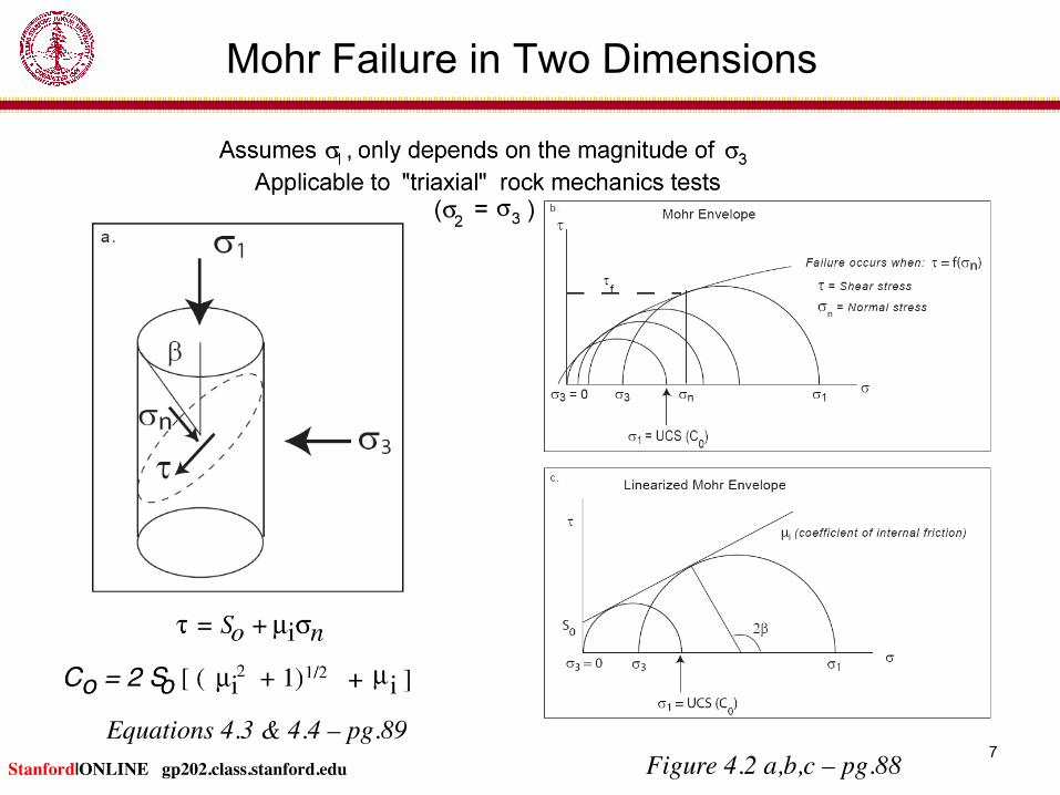
Mohr Failure in Two Dimensions
Equations 4.3 & 4.4 – pg.89 Figure 4.2 a,b,c – pg.88 Stanford|ONLINE gp202.class.stanford.edu
7

Practical Guide to Determination of C0 and µi
nn
i 21−
=µ
Figure 4.3 b – pg.90
Equation 4.5 – pg.89
Stanford|ONLINE gp202.class.stanford.edu
8
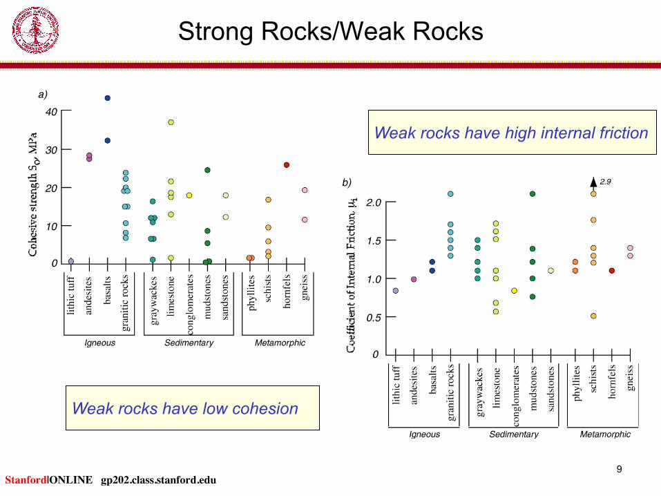
Strong Rocks/Weak Rocks
Weak rocks have low cohesion
Weak rocks have high internal friction
Stanford|ONLINE gp202.class.stanford.edu
9

More Complex Failure Criterion that Describe Rock Strength in Compression
Over the years, comprehensive laboratory studies have yielded a variety of failure criterion to describe rock strength in compression which are summarized below. However, to quote Mark Twain,
The efforts of many researchers have already cast much darkness on the subject, and it is likely that, if they continue, we will soon know nothing about it at all.
This statement, reflective of Twain’s inherent cynicism, is unfortunately
applicable of the degree to which concepts about rock failure based on laboratory rock mechanics has made the subject of rock strength sufficiently complex that it can almost never be practically applied in case studies. Thus, the most important thing to keep in mind is that
Strong rock is strong, weak rock isn't
Our first goal is to capture the essential rock strength. Using advanced
failure criterion to describe rock strength is a worthy, but secondary, objective.
Stanford|ONLINE gp202.class.stanford.edu
10

Strength Criteria in Which the Stress at Failure, σ1, Depends Only on σ3
Linearized Mohr-Coulomb criterion (Jaeger and Cook, 1979)
Empirical criterion of Hoek and Brown (1980)
where m and s are constants that depend on the properties of the rock and on the extent to which it was broken before being subjected to the failure.
€
σ1 = qσ3 + C0
€
q = ( µ2 +1 + µ)2
€
σ1 =σ 3 + C0 mσ 3
C0
+ s
Equations 4.6 - 4.8 – pg.93
Equation 4.9 – pg.98
€
tanΦ = µ
Stanford|ONLINE gp202.class.stanford.edu
11

Polyaxial Strength Criteria (The Stress at Failure, σ1, Depends on σ2)
Modified Lade criterion (Ewy, 1998) – A personal favorite
€
I1'( )3
I3' − 27
#
$
% %
&
'
( (
I1'( )m
ρa
#
$
% %
&
'
( (
=η
€
I1' = (σ1 + S ) + (σ 2 + S ) + (σ 3 + S )I3' = (σ1 + S )(σ 2 + S )(σ 3 + S )
€
η = 4µ2 9 µ2 +1 − 7µ
µ2 +1 − µ
€
S = So /tanΦ
Equations 4.13 - 4.17 – pg.100
Among Failure Criterion that are Functions of Three Principal Stresses
Stanford|ONLINE gp202.class.stanford.edu
12

Failure Envelopes in Stress Space
Figure 4.6 – pg.94 Stanford|ONLINE gp202.class.stanford.edu
13

Rock Strength is a Function of Simple Effective Stress
Figure 4.11 a-d – pg.105 Stanford|ONLINE gp202.class.stanford.edu
14
Section 1 • Compressive Strength • Strength Criterion Section 2 • Strength Anisotropy • Shear Enhanced Compaction • Strength from Logs Section 3 • Tensile Strength • Hydraulic Fracture Propagation • Vertical Growth of Hydraulic Fractures
Stanford|ONLINE gp202.class.stanford.edu
Outline
15

Strength Anisotropy
( )( ) ββµ−
σµ+=σ=σ
2sincot1S2
ww
3ww31
if w
w12tanµ
−=β
σ1min = σ3 + 2 Sw + µwσ 3( ) µw
2 +1( )12 + µw
"
# $
%
& '
Parallel Planes of Weakness (Bedding/Foliation)
Equations 4.33 - 4.34 – pg.107
Stanford|ONLINE gp202.class.stanford.edu
16

Highly Foliated Gneiss
Stanford|ONLINE gp202.class.stanford.edu
17

Cam-Clay Model: Elliptical End Caps
Figure 4.19 – pg.119
Shear Enhanced Compaction (End Cap)
Stanford|ONLINE gp202.class.stanford.edu
18
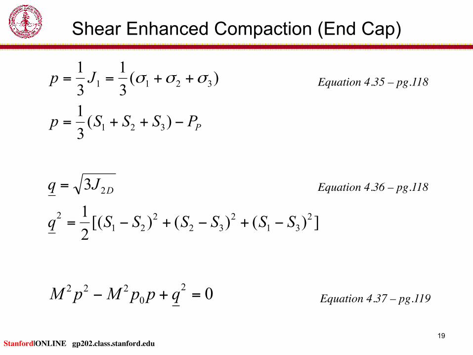
PPSSSp
Jp
−++=
++==
)(31
)(31
31
321
3211 σσσ
])()()[(21
3
231
232
221
2
2
SSSSSSq
Jq D
−+−+−=
=
020
222 =+− qppMpM Equation 4.37 – pg.119
Equation 4.36 – pg.118
Equation 4.35 – pg.118
Stanford|ONLINE gp202.class.stanford.edu
19
Shear Enhanced Compaction (End Cap)

Shear Enhanced Compaction (End Cap)
0
100
200
300
0 100 200 300 400
((Sh+SH+Sv)/3)-Pp (MPa)
Sv-Sh
(MPa)
Adamswiller (W97)
Berea (W97)
Boise-2 (W97)
Darley Dale (W97)
Rothbach-1 (W97)
Rothbach-2 (W97)
Kayenta (W97)
Navajo (D73)
Kayenta (D73)
Cutler (D97)
Adamswiller (W97)
Berea (W97)
Boise (W97)
Darley Dale (W97)
Rothbach-2 (W97)
Kayenta (W97)
Berea (J&T79)
Bad Durck (S98)
Castlegate (B&J98)
Berea (H63)
Galesville (B81)
Berea (K91)
Vosges (F98)
Red Wildmoor (Pap00)
21%
23%
35%
20%
21%
15%
Figure 4.20 – pg.120 Stanford|ONLINE gp202.class.stanford.edu
20

End Caps and Lab Tests
Figure 4.19 – pg.119 Stanford|ONLINE gp202.class.stanford.edu
21
Deformation Analysis in Reservoir Space (DARS)
To understand the deformation mechanisms of a producing reservoir utilizing relatively simple laboratory tests and in situ measurements
DARS is a formalism for estimating the evolution of
porosity, permeability and the potential for induced normal faulting in a producing reservoir
Stanford|ONLINE gp202.class.stanford.edu
22
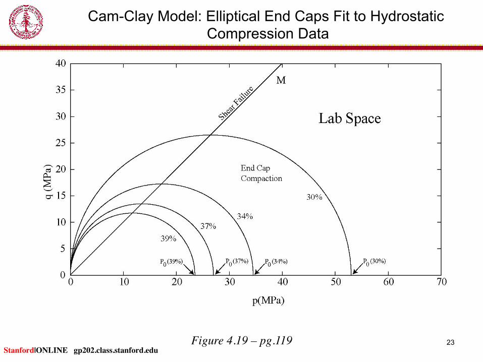
Figure 4.19 – pg.119 Stanford|ONLINE gp202.class.stanford.edu
Cam-Clay Model: Elliptical End Caps Fit to Hydrostatic Compression Data
23

Lab Space
Reservoir Space
DARS
Pp (MPa)
p (MPa)
q (M
Pa)
Shm
in (M
Pa)
Stanford|ONLINE gp202.class.stanford.edu
24
Deformation Analysis in Reservoir Space (DARS)

Lab Space
Reservoir Space
DARS
Pp (MPa)
p (MPa)
q (M
Pa)
Shm
in (M
Pa)
Stanford|ONLINE gp202.class.stanford.edu
25
Deformation Analysis in Reservoir Space (DARS)

26

Gulf of Mexico Field X
Stanford|ONLINE gp202.class.stanford.edu
27
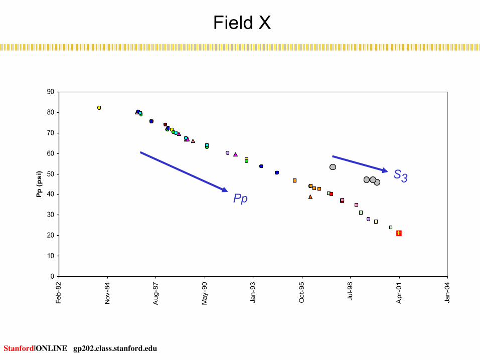
Pp
S3
0
10
20
30
40
50
60
70
80
90
Feb-82
Nov-84
Aug-87
May-90
Jan-93
Oct-95
Jul-98
Apr-01
Jan-04
Pp (p
si)
Pp
S3
Field X
Stanford|ONLINE gp202.class.stanford.edu
28

29

Initial porosity 26.5%
Stanford|ONLINE gp202.class.stanford.edu
30
DARS

Estimating Rock Strength From Geophysical Logs
• Why? • What? • How Well Does it Work?
• Be Careful Out There!
Stanford|ONLINE gp202.class.stanford.edu
31

Figure 4.15 – pg.111 Figure 4.16 – pg.112 Figure 4.14 – pg.110

Eq. No. UCS, MPa Region Where Developed General Comments Reference 1 0.035 Vp – 31.5 Thuringia, Germany - (Freyburg 1972) 2 1200 exp(-0.036Δt) Bowen Basin, Australia
Fine grained, both consolidated and unconsolidated sandstones with wide porosity range
(McNally 1987)
3 1.4138×10⁷ Δt-3 Gulf Coast Weak and unconsolidated sandstones Unpublished
4 3.3×10⁻²⁰ ρ2Vp4 [(1+ν)/(1-ν)]2(1-2ν) [1+ 0.78Vclay] Gulf Coast Applicable to sandstones
with UCS >30 MPa (Fjaer, Holt et al. 1992) 5 1.745×10⁻⁹ ρVp
2 - 21 Cook Inlet, Alaska Coarse grained sands and conglomerates (Moos, Zoback et al. 1999)
6 42.1 exp(1.9×10⁻¹¹ ρVp2) Australia Consolidated sandstones with
0.05<φ<0.12 and UCS>80MPa
Unpublished
7 3.87 exp(1.14×10⁻¹⁰ ρVp2) Gulf of Mexico - Unpublished
8 46.2 exp(0.000027E) - - Unpublished 9 A (1-Bφ)2 Sedimentary basins
worldwide Very clean, well consolidated sandstones with φ<0.30
(Vernik, Bruno et al. 1993)
10 277 exp(-10φ) - Sandstones with 2<UCS<360MPa and 0.002<φ<0.33
Unpublished
Units used: Vp (m/s), Δt (µs/ft), ρ (kg/m3), Vclay (fraction), E (MPa), φ (fraction)
Table 4.1 – pg.113
Sandstone
Stanford|ONLINE gp202.class.stanford.edu
33
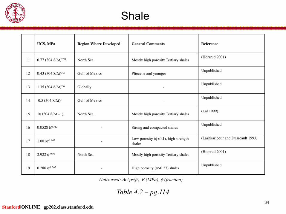
UCS, MPa Region Where Developed General Comments Reference
11 0.77 (304.8/Δt)2.93 North Sea Mostly high porosity Tertiary shales (Horsrud 2001)
12 0.43 (304.8/Δt)3.2 Gulf of Mexico Pliocene and younger Unpublished
13 1.35 (304.8/Δt)2.6 Globally - Unpublished
14 0.5 (304.8/Δt)3 Gulf of Mexico - Unpublished
15 10 (304.8/Δt –1) North Sea Mostly high porosity Tertiary shales (Lal 1999)
16 0.0528 E0.712 - Strong and compacted shales Unpublished
17 1.001φ-1.143 - Low porosity (φ<0.1), high strength shales
(Lashkaripour and Dusseault 1993)
18 2.922 φ–0.96 North Sea Mostly high porosity Tertiary shales (Horsrud 2001)
19 0.286 φ-1.762 - High porosity (φ>0.27) shales Unpublished
Table 4.2 – pg.114
Units used: Δt (µs/ft), E (MPa), φ (fraction)
Shale
Stanford|ONLINE gp202.class.stanford.edu
34
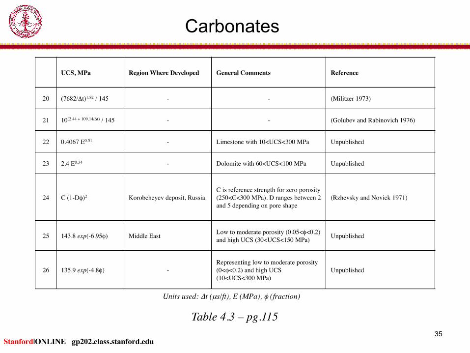
UCS, MPa Region Where Developed General Comments Reference 20 (7682/Δt)1.82 / 145 - - (Militzer 1973) 21 10(2.44 + 109.14/Δt) / 145 - - (Golubev and Rabinovich 1976) 22 0.4067 E0.51 - Limestone with 10<UCS<300 MPa Unpublished 23 2.4 E0.34 - Dolomite with 60<UCS<100 MPa Unpublished
24 C (1-Dφ)2 Korobcheyev deposit, Russia C is reference strength for zero porosity (250<C<300 MPa). D ranges between 2 and 5 depending on pore shape (Rzhevsky and Novick 1971)
25 143.8 exp(-6.95φ) Middle East Low to moderate porosity (0.05<φ<0.2) and high UCS (30<UCS<150 MPa) Unpublished
26 135.9 exp(-4.8φ) - Representing low to moderate porosity (0<φ<0.2) and high UCS (10<UCS<300 MPa)
Unpublished
Table 4.3 – pg.115
Units used: Δt (µs/ft), E (MPa), φ (fraction)
Carbonates
Stanford|ONLINE gp202.class.stanford.edu
35

Φ, degree General Comments Reference
27 sin-1 ((Vp-1000) / (Vp+1000)) Applicable to shale (Lal 1999)
28 70 - 0.417GR Applicable to shaly sedimentary rocks with 60< GR <120
Unpublished
Table 4.4 – pg.116
Units used: Vp (m/s), GR (API)
Coefficient of Internal Friction
Stanford|ONLINE gp202.class.stanford.edu
36
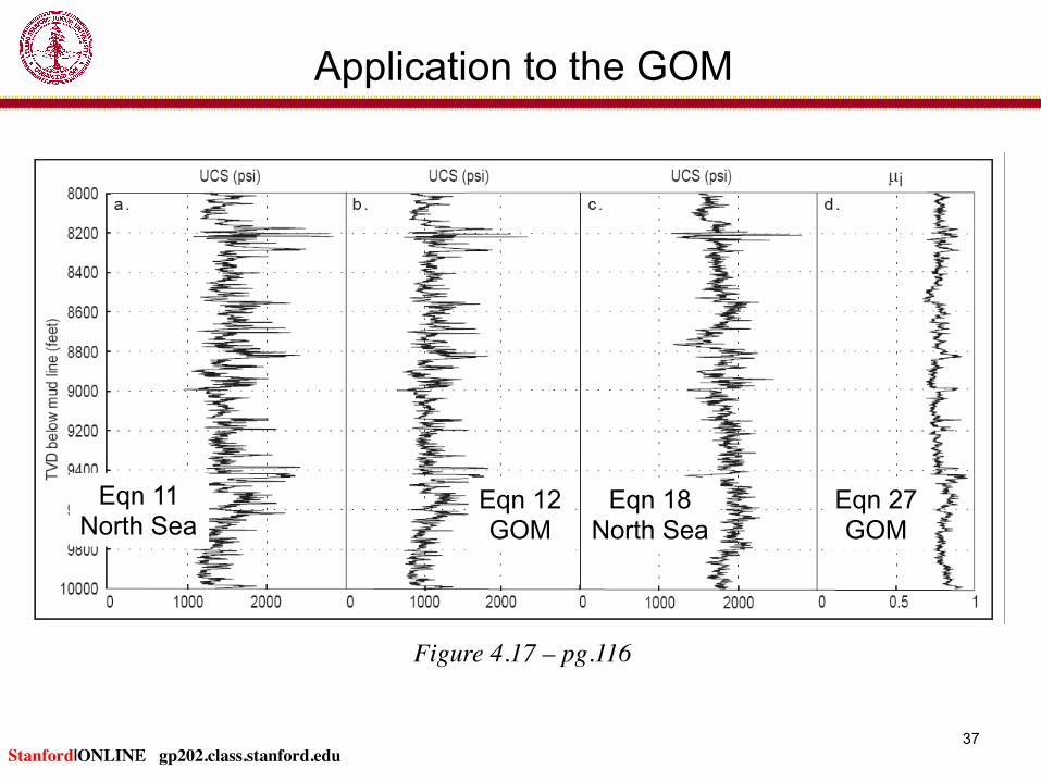
Figure 4.17 – pg.116
Application to the GOM
Eqn 11 North Sea
Eqn 12 GOM
Eqn 18 North Sea
Eqn 27 GOM
Stanford|ONLINE gp202.class.stanford.edu
37
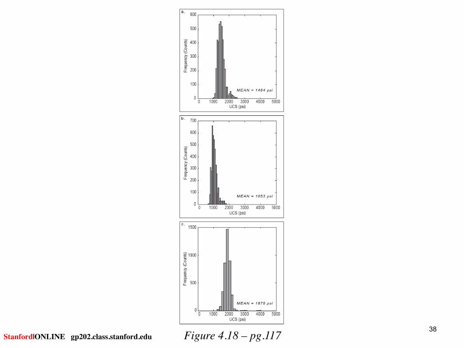
Figure 4.18 – pg.117 Stanford|ONLINE gp202.class.stanford.edu
38

Organic Rich Shales
• Bedding plane and sample cylinder axis is either parallel (horizontal samples) or perpendicular (vertical samples)
• 3-10 % porosity • All room dry, room temperature experiments
Sample group Clay Carbonate QFP TOC (wt%)
Barnett-dark 29-43 0-6 48-59 4.1-5.8
Barnett-light 2-7 37-81 16-53 0.4-1.3
Haynesville-dark 36-39 20-23 31-35 3.7-4.1
Haynesville-light 20-22 49-53 23-24 1.7-1.8
Fort St. John 32-39 3-5 54-60 1.6-2.2
Eagle Ford-dark 12-21 46-54 22-29 4.4-5.7
Eagle Ford-light 6-14 63-78 11-18 1.9-2.5
Stanford|ONLINE gp202.class.stanford.edu
39

0
10
20
30
40
50
60
70
80
0 10 20 30 40 50
Clay Content [%]
Youn
g's
Mod
ulus
[MPa
]
Barnett Dark Barnett LightHaynesville Dark Haynesville LightFt. St. John
Young’s Modulus
Bed-‐Parallel Samples
• Modulus correlate with clay content and porosity
• Bedding parallel samples are systematically stiffer
0
50
100
150
200
250
0 10 20 30 40 50
Approximate Clay Content [%]
UC
S [M
Pa]
0
0.2
0.4
0.6
0.8
1 Coefficient of Internal Friction
Unconfined Compressive StrengthInternal Frictional Coefficient
Strength
Youn
g’s
Mod
ulus
(GP
a)
UC
S (M
Pa)
Approximate Clay Content (%) Approximate Clay Content (%)
• Strength decreases with clay content
• Internal friction coefficient decreases from 0.9 to 0.2
Stanford|ONLINE gp202.class.stanford.edu
40

Section 1 • Compressive Strength • Strength Criterion Section 2 • Strength Anisotropy • Shear Enhanced Compaction • Strength from Logs Section 3 • Tensile Strength • Hydraulic Fracture Propagation • Vertical Growth of Hydraulic Fractures
Stanford|ONLINE gp202.class.stanford.edu
Outline
41

Stanford|ONLINE gp202.class.stanford.edu
42
Rock Strength Measurement
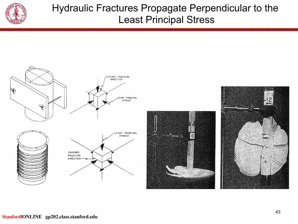
Hydraulic Fractures Propagate Perpendicular to the Least Principal Stress
Stanford|ONLINE gp202.class.stanford.edu
43
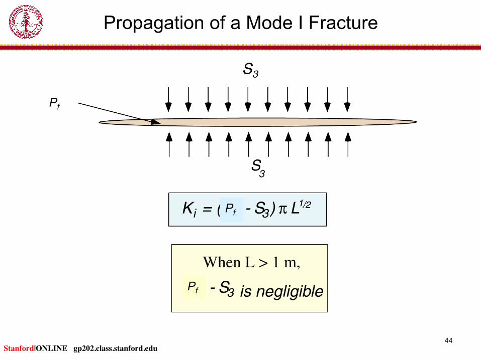
Propagation of a Mode I Fracture
Pf
Pf
Pf
Stanford|ONLINE gp202.class.stanford.edu
44

Tensile Strength of Mode I Cracks in Sedimentary Rocks is Irrelevant for Fracture Propagation*
*Once the fracture begins to propagate
Stanford|ONLINE gp202.class.stanford.edu
45

What Controls the Vertical Growth of Hydraulic Fractures?
46

Case 1 – A Strong Contrast Between the Magnitude of Shmin Within the Target Formation Prevents Vertical Propagation
3000 6000 psi
Stanford|ONLINE gp202.class.stanford.edu
47
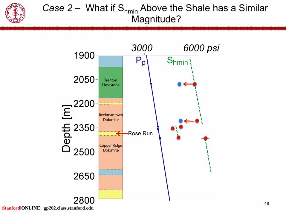
3000 6000 psi
Case 2 – What if Shmin Above the Shale has a Similar Magnitude?
Stanford|ONLINE gp202.class.stanford.edu
48

Multi-Stage Hydraulic Fracturing
Microseismic Events
Hydraulic Fractures
Well
Stanford|ONLINE gp202.class.stanford.edu
49

Fisher (2010)
Tendency for Upward Vertical Hydraulic Fracture Growth in the Marcellus Shale
Stanford|ONLINE gp202.class.stanford.edu
50

http://nwis.waterdata.usgs.gov/nwis/inventory
Tendency for Downward Growth of Hydraulic Fractures in the Barnett Shale into the Ellenburger Limestone
Fisher (2010)
Stanford|ONLINE gp202.class.stanford.edu
51

What Controls the Vertical Growth of Hydraulic Fractures?
The Variation of the S3 (Shmin)
With Depth
Measure It!
52
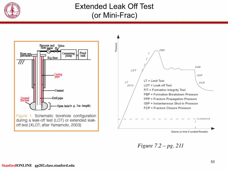
Extended Leak Off Test (or Mini-Frac)
Figure 7.2 – pg. 211
Stanford|ONLINE gp202.class.stanford.edu
53

Case 1 – A Strong Contrast Between the Magnitude of Shmin Within the Target Formation Prevents Vertical Propagation
3000 6000 psi
Stanford|ONLINE gp202.class.stanford.edu
54