residential curbside characterization
TRANSCRIPT
Residential Curbside Characterization
October 2018 FINAL
Seattle | Oakland
www.cascadiaconsulting.com

This page intentionally left blank
King County Waste Monitoring 2018 Task 1: Residential Curbside Characterization
Table of Contents 1. Introduction and Summary .............................................................................................. 1
2. Summary of Methodology ............................................................................................... 6
Commonly Used Terms .......................................................................................................................... 6
Study Design ........................................................................................................................................... 7
Collect Data ............................................................................................................................................ 7
Changes to the Methodology from the Previous Study ......................................................................... 8
3. Findings ........................................................................................................................... 9
Interpreting the Composition Results .................................................................................................... 9
Results .................................................................................................................................................. 10
Comparisons to Previous Organics Studies .......................................................................................... 49
Appendix A: Material Type Definitions ................................................................................. 52
Appendix B: Study Design .................................................................................................... 54
Appendix C. Greenhouse Gas Impacts .................................................................................. 63
Appendix D: Calculations ..................................................................................................... 68
Appendix E: Example Field Forms ........................................................................................ 74
Appendix F: Detailed Composition Tables ............................................................................ 80
King County Waste Monitoring 2018 Task 1: Residential Curbside Characterization
Tables Table 1. Detailed Composition, Single-family Generation ............................................................................................. 2 Table 2. Key Organics Metrics ....................................................................................................................................... 3 Table 3. Jurisdiction Service Schedule and Service Type ............................................................................................... 7 Table 4. Top Five Material Types, Single-family Generation ....................................................................................... 11 Table 5. Detailed Composition, Single-family Generation ........................................................................................... 12 Table 6. Top Five Material Types, Single-family Garbage ............................................................................................ 14 Table 7. Detailed Composition, Single-family Garbage ............................................................................................... 15 Table 8. Top Five Material Types, Single-family Recycling .......................................................................................... 17 Table 9. Detailed Composition, Single-family Recycling .............................................................................................. 18 Table 10. Top Five Material Types, Single-family Organics ......................................................................................... 23 Table 11. Detailed Composition, Single-family Organics ............................................................................................. 24 Table 12. Organics Set-out Rate by Service Schedule and Customer Type ................................................................. 26 Table 13. Comparison of Key Organics Metrics by Service Type ................................................................................. 28 Table 14. Comparison of Key Organics Metrics by Service Type ................................................................................. 28 Table 15. Comparison of Key Organics Metrics by Service Schedule .......................................................................... 28 Table 16. Comparison of Key Organics Metrics by Service Schedule .......................................................................... 28 Table 17: Comparison of Key Data between 2011 and 2017 ...................................................................................... 49 Table 18. Set-out Rate by Field Season ....................................................................................................................... 50 Table 19. Household Food Scraps and Compostable Paper Capture Rates ................................................................. 50 Table 20. T-test Results................................................................................................................................................ 51 Table 21. 2017 Sampling Schedule .............................................................................................................................. 54 Table 22. Service Types and Service Schedules by City ............................................................................................... 57 Table 23: Jurisdictions with Routes Randomly Selected for Sampling in 2017 ........................................................... 58 Table 24. Material types Included in the GHG Analysis ............................................................................................... 63 Table 25: Modeled Transportation Distances ............................................................................................................. 64 Table 26. Estimated GHG Reductions from Recycling and Organics Service ............................................................... 65 Table 27. Recovered Tons at Each Modeled Diversion Level ...................................................................................... 66 Table 28. Change in MtCO2e at Each Modeled Diversion Level .................................................................................. 67 Table 29. Detailed Composition, Single-family Embedded Service ............................................................................. 80 Table 30. Detailed Composition, Single-family Subscription Service ........................................................................... 80 Table 31. Detailed Composition, Single-family Weekly Collection .............................................................................. 81 Table 32. Detailed Composition, Single-family Every Other Week Collection ............................................................. 81 Table 33. Detailed Composition, Single-family Embedded Service with Weekly Collection ....................................... 82 Table 34. Detailed Composition, Single-family Embedded Service with EOW Collection ........................................... 82 Table 35. Detailed Composition, Single-family Subscription Service with Weekly Collection ..................................... 83 Table 36. Detailed Composition, Single-family Subscription Service with EOW Collection......................................... 83
King County Waste Monitoring 2018 Task 1: Residential Curbside Characterization
Figures Figure 1. Recycling Set-out Rate by Service Schedule ................................................................................................... 3 Figure 2. Organics Set-out Rate by Service Schedule and Service Type ........................................................................ 3 Figure 3. Recyclables Capture Rate by Service Schedule ............................................................................................... 4 Figure 4. Household Food Scraps and Compostable Paper Capture Rate Over Time ................................................... 4 Figure 5. Recycling Contamination Rate Distribution .................................................................................................... 4 Figure 6. Organics Contamination Rate Distribution ..................................................................................................... 5 Figure 7. Annual Tons by Material Stream .................................................................................................................. 10 Figure 8. Composition by Material Class, Single-family Generation ............................................................................ 11 Figure 9. Annual Generated Pounds per Household by Services Utilized ................................................................... 13 Figure 10. Composition by Material Class, Single-family Garbage .............................................................................. 14 Figure 11. Annual Garbage Pounds per Household Rates by Services Utilized ........................................................... 16 Figure 12. Composition by Material Class, Single-family Recycling ............................................................................. 17 Figure 13. Annual Recycling Pounds per Household by Services Utilized ................................................................... 19 Figure 14. Annual Recycling Pounds per Household by Service Schedule ................................................................... 19 Figure 15. Recycling Set-out Rate by Service Schedule ............................................................................................... 20 Figure 16. Recyclable Paper Participation Rate by Service Schedule .......................................................................... 20 Figure 17. Recyclable Plastic Participation Rate by Service Schedule ......................................................................... 21 Figure 18. Recyclable Metal Participation Rate by Service Schedule .......................................................................... 21 Figure 19. Recyclable Glass Participation Rate by Service Schedule ........................................................................... 22 Figure 20. Composition by Material Class, Single-family Organics .............................................................................. 23 Figure 21. Annual Organics Pounds per Household by Services Utilized .................................................................... 25 Figure 22. Annual Organics Pounds per Household by Service Schedule and Service Type ........................................ 25 Figure 23. Organics Set-out Rate by Service Schedule and Service Type .................................................................... 26 Figure 24. Food Scrap and Compostable Paper Participation Rate ............................................................................. 27 Figure 25. Recyclables Capture Rate by Service Schedule ........................................................................................... 29 Figure 26. Recyclables Capture Rate ........................................................................................................................... 30 Figure 27. Recyclables Capture Rate Weekly Service .................................................................................................. 30 Figure 28. Recyclables Capture Rate Every Other Week Service ................................................................................. 30 Figure 29. Recyclable Paper Capture Rate by Service Schedule .................................................................................. 31 Figure 30. Recyclable Paper Capture Rate ................................................................................................................... 31 Figure 31. Recyclable Paper Capture Rate, Weekly Service ........................................................................................ 32 Figure 32. Recyclable Paper Capture Rate EOW Service ............................................................................................. 32 Figure 33. Recyclable Plastic Capture Rate by Service Schedule ................................................................................. 32 Figure 34. Recyclable Plastic Capture Rate .................................................................................................................. 33 Figure 35. Recyclable Plastic Capture Rate Weekly Service ........................................................................................ 33 Figure 36. Recyclable Plastic Capture Rate EOW Service ............................................................................................ 33 Figure 37. Recyclable Metal Capture Rate by Service Schedule .................................................................................. 33 Figure 38. Recyclable Metal Capture Rate ................................................................................................................... 34 Figure 39. Recyclable Metal Capture Rate Weekly Service ......................................................................................... 34 Figure 40. Recyclable Metal Capture Rate EOW Service ............................................................................................. 34 Figure 41. Recyclable Glass Capture Rate by Service Schedule ................................................................................... 35 Figure 42. Recyclable Glass Capture Rate .................................................................................................................... 35 Figure 43. Recyclable Glass Capture Rate Weekly Service .......................................................................................... 36 Figure 44. Recyclable Glass Capture Rate EOW Service .............................................................................................. 36 Figure 45. Recyclables Diversion Efficiency ................................................................................................................. 37 Figure 46. Recyclable Paper Diversion Efficiency ........................................................................................................ 37 Figure 47. Recyclable Plastic Diversion Efficiency ....................................................................................................... 38 Figure 48. Recyclable Metal Diversion Efficiency ........................................................................................................ 38
King County Waste Monitoring 2018 Task 1: Residential Curbside Characterization
Figure 49. Recyclable Glass Diversion Efficiency ......................................................................................................... 39 Figure 50. All Compostables Capture Rate by Service Schedule and Service Type ..................................................... 40 Figure 51. All Compostables Capture Rate .................................................................................................................. 41 Figure 52. All Compostables Capture Rate Embedded Weekly ................................................................................... 42 Figure 53. All Compostables Capture Rate Embedded Every Other Week .................................................................. 42 Figure 54. All Compostables Capture Rate Subscription Weekly ................................................................................ 42 Figure 55. All Compostables Capture Rate Subscription Every Other Week ............................................................... 42 Figure 56. Food Scraps and Compostable Paper Capture Rate, by Service Schedule and Service Type ..................... 43 Figure 57. Food Scraps and Compostable Paper Capture Rate ................................................................................... 43 Figure 58. FSCP Capture Rate Embedded Weekly Service ........................................................................................... 44 Figure 59. FSCP Capture Rate Embedded Every Other Week Service ......................................................................... 44 Figure 60. FSCP Capture Rate Subscription Weekly Service ........................................................................................ 44 Figure 61. FSCP Capture Rate Subscription Every Other Week Service ....................................................................... 44 Figure 62. All Compostables Diversion Efficiency ........................................................................................................ 45 Figure 63. Food Scraps and Compostable Paper Diversion Efficiency ......................................................................... 45 Figure 64. Recycling Contamination Rate Distribution ................................................................................................ 46 Figure 65. Recycling Contamination Rate Distribution Weekly Service....................................................................... 47 Figure 66. Recycling Contamination Rate Distribution Every Other Week Service ..................................................... 47 Figure 67. Organics Contamination Rate Distribution ................................................................................................. 47 Figure 68. Organics Contamination Rate Distribution Embedded Weekly Service ..................................................... 48 Figure 69. Organics Contamination Rate Distribution Embedded Every Other Week Service .................................... 48 Figure 70. Organics Contamination Rate Distribution Subscription Weekly Service ................................................... 48 Figure 71. Organics Contamination Rate Distribution Subscription Every Other Week Service ................................. 48 Figure 72. Household Food Scraps and Compostable Paper Capture Rate Over Time ............................................... 51 Figure 73. Organics Route Data Collection Area Illustration ....................................................................................... 59 Figure 74. Overview of the Sample Selection and Sorting Process ............................................................................. 62 Figure 75. Set Out Count Form .................................................................................................................................... 75 Figure 76. Sample Label ............................................................................................................................................... 76 Figure 77. Sample Tally Sheet ...................................................................................................................................... 77 Figure 78. Customer Hand Out .................................................................................................................................... 78 Figure 79. Customer Interaction Tracking Form .......................................................................................................... 79
1 King County Waste Monitoring 2018 Task 1: Residential Curbside Characterization
1. Introduction and Summary
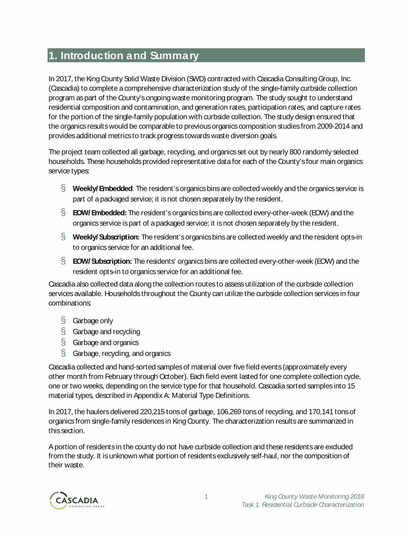
In 2017, the King County Solid Waste Division (SWD) contracted with Cascadia Consulting Group, Inc. (Cascadia) to complete a comprehensive characterization study of the single-family curbside collection program as part of the County's ongoing waste monitoring program. The study sought to understand residential composition and contamination, and generation rates, participation rates, and capture rates for the portion of the single-family population with curbside collection. The study design ensured that the organics results would be comparable to previous organics composition studies from 2009-2014 and provides additional metrics to track progress towards waste diversion goals.
The project team collected all garbage, recycling, and organics set out by nearly 800 randomly selected households. These households provided representative data for each of the County’s four main organics service types:
§ Weekly/Embedded: The resident’s organics bins are collected weekly and the organics service is part of a packaged service; it is not chosen separately by the resident.
§ EOW/Embedded: The resident’s organics bins are collected every-other-week (EOW) and the organics service is part of a packaged service; it is not chosen separately by the resident.
§ Weekly/Subscription: The resident’s organics bins are collected weekly and the resident opts-in to organics service for an additional fee.
§ EOW/Subscription: The residents’ organics bins are collected every-other-week (EOW) and the resident opts-in to organics service for an additional fee.
Cascadia also collected data along the collection routes to assess utilization of the curbside collection services available. Households throughout the County can utilize the curbside collection services in four combinations:
§ Garbage only § Garbage and recycling § Garbage and organics § Garbage, recycling, and organics
Cascadia collected and hand-sorted samples of material over five field events (approximately every other month from February through October). Each field event lasted for one complete collection cycle, one or two weeks, depending on the service type for that household. Cascadia sorted samples into 15 material types, described in Appendix A: Material Type Definitions.
In 2017, the haulers delivered 220,215 tons of garbage, 106,269 tons of recycling, and 170,141 tons of organics from single-family residences in King County. The characterization results are summarized in this section.
A portion of residents in the county do not have curbside collection and these residents are excluded from the study. It is unknown what portion of residents exclusively self-haul, nor the composition of their waste.
2 King County Waste Monitoring 2018 Task 1: Residential Curbside Characterization
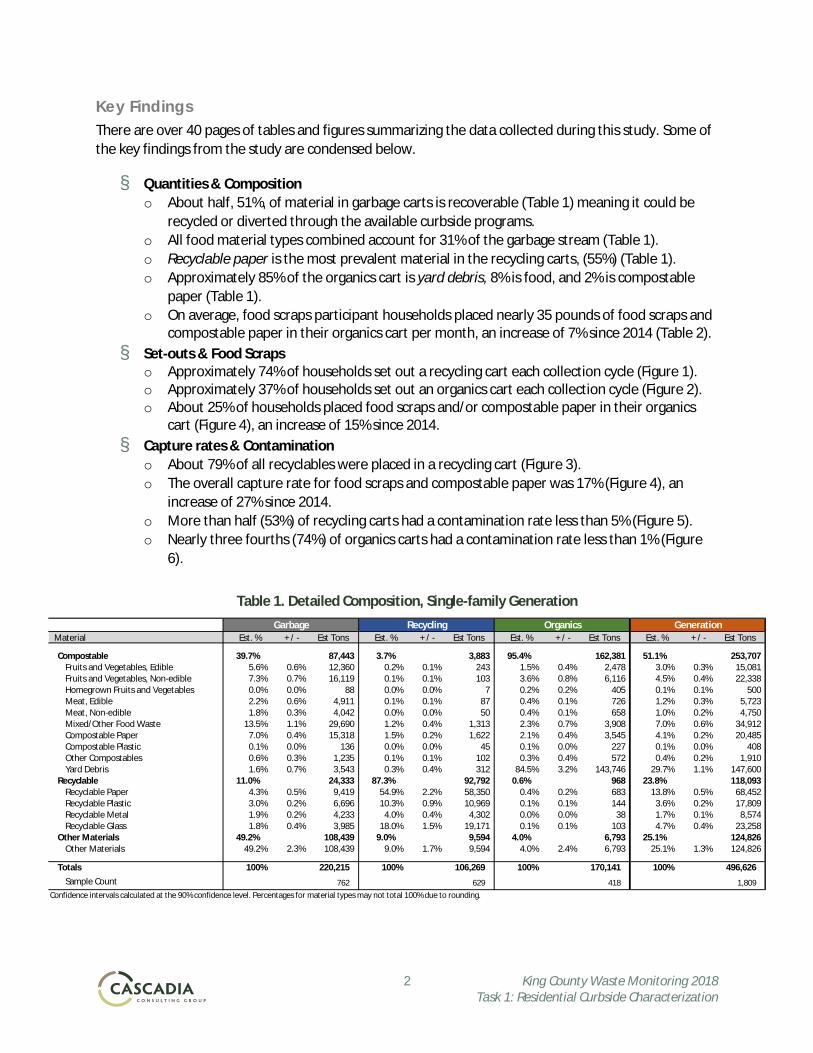
Key Findings There are over 40 pages of tables and figures summarizing the data collected during this study. Some of the key findings from the study are condensed below.
§ Quantities & Composition o About half, 51%, of material in garbage carts is recoverable (Table 1) meaning it could be
recycled or diverted through the available curbside programs. o All food material types combined account for 31% of the garbage stream (Table 1). o Recyclable paper is the most prevalent material in the recycling carts, (55%) (Table 1). o Approximately 85% of the organics cart is yard debris, 8% is food, and 2% is compostable
paper (Table 1). o On average, food scraps participant households placed nearly 35 pounds of food scraps and
compostable paper in their organics cart per month, an increase of 7% since 2014 (Table 2). § Set-outs & Food Scraps
o Approximately 74% of households set out a recycling cart each collection cycle (Figure 1). o Approximately 37% of households set out an organics cart each collection cycle (Figure 2). o About 25% of households placed food scraps and/or compostable paper in their organics
cart (Figure 4), an increase of 15% since 2014. § Capture rates & Contamination
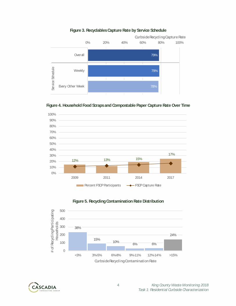
o About 79% of all recyclables were placed in a recycling cart (Figure 3). o The overall capture rate for food scraps and compostable paper was 17% (Figure 4), an
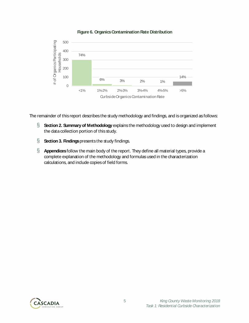
increase of 27% since 2014. o More than half (53%) of recycling carts had a contamination rate less than 5% (Figure 5). o Nearly three fourths (74%) of organics carts had a contamination rate less than 1% (Figure
6).
Table 1. Detailed Composition, Single-family Generation
Garbage Recycling Organics Generation Material Est. % + / - Est Tons Est. % + / - Est Tons Est. % + / - Est Tons Est. % + / - Est Tons
Compostable 39.7% 87,443 3.7% 3,883 95.4% 162,381 51.1% 253,707 Fruits and Vegetables, Edible 5.6% 0.6% 12,360 0.2% 0.1% 243 1.5% 0.4% 2,478 3.0% 0.3% 15,081 Fruits and Vegetables, Non-edible 7.3% 0.7% 16,119 0.1% 0.1% 103 3.6% 0.8% 6,116 4.5% 0.4% 22,338 Homegrown Fruits and Vegetables 0.0% 0.0% 88 0.0% 0.0% 7 0.2% 0.2% 405 0.1% 0.1% 500 Meat, Edible 2.2% 0.6% 4,911 0.1% 0.1% 87 0.4% 0.1% 726 1.2% 0.3% 5,723 Meat, Non-edible 1.8% 0.3% 4,042 0.0% 0.0% 50 0.4% 0.1% 658 1.0% 0.2% 4,750 Mixed/Other Food Waste 13.5% 1.1% 29,690 1.2% 0.4% 1,313 2.3% 0.7% 3,908 7.0% 0.6% 34,912 Compostable Paper 7.0% 0.4% 15,318 1.5% 0.2% 1,622 2.1% 0.4% 3,545 4.1% 0.2% 20,485 Compostable Plastic 0.1% 0.0% 136 0.0% 0.0% 45 0.1% 0.0% 227 0.1% 0.0% 408 Other Compostables 0.6% 0.3% 1,235 0.1% 0.1% 102 0.3% 0.4% 572 0.4% 0.2% 1,910 Yard Debris 1.6% 0.7% 3,543 0.3% 0.4% 312 84.5% 3.2% 143,746 29.7% 1.1% 147,600
Recyclable 11.0% 24,333 87.3% 92,792 0.6% 968 23.8% 118,093 Recyclable Paper 4.3% 0.5% 9,419 54.9% 2.2% 58,350 0.4% 0.2% 683 13.8% 0.5% 68,452 Recyclable Plastic 3.0% 0.2% 6,696 10.3% 0.9% 10,969 0.1% 0.1% 144 3.6% 0.2% 17,809 Recyclable Metal 1.9% 0.2% 4,233 4.0% 0.4% 4,302 0.0% 0.0% 38 1.7% 0.1% 8,574 Recyclable Glass 1.8% 0.4% 3,985 18.0% 1.5% 19,171 0.1% 0.1% 103 4.7% 0.4% 23,258
Other Materials 49.2% 108,439 9.0% 9,594 4.0% 6,793 25.1% 124,826 Other Materials 49.2% 2.3% 108,439 9.0% 1.7% 9,594 4.0% 2.4% 6,793 25.1% 1.3% 124,826
Totals 100% 220,215 100% 106,269 100% 170,141 100% 496,626Sample Count 762 629 418 1,809
Confidence intervals calculated at the 90% confidence level. Percentages for material types may not total 100% due to rounding.
3 King County Waste Monitoring 2018 Task 1: Residential Curbside Characterization
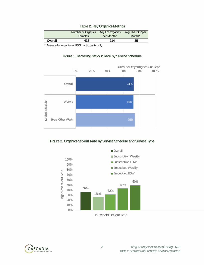
Table 2. Key Organics Metrics
Figure 1. Recycling Set-out Rate by Service Schedule
Figure 2. Organics Set-out Rate by Service Schedule and Service Type
Number of Organics Samples
Avg. Lbs Organics per Month*
Avg. Lbs FSCP per Month*
Overall 418 214 35* Average for organics or FSCP participants only.
74%
74%
75%
0% 20% 40% 60% 80% 100%
Overall
Weekly
Every Other WeekServ
ice
Sche
dule
Curbside Recycling Set-Out Rate
37%
26%32%
43%50%
0%
10%
20%
30%
40%
50%
60%
70%
80%
90%
100%
Household Set-out Rate
Org
anic
s Set
-out
Rat
e
Overall
Subscription Weekly
Subscription EOW
Embedded Weekly
Embedded EOW
4 King County Waste Monitoring 2018 Task 1: Residential Curbside Characterization
Figure 3. Recyclables Capture Rate by Service Schedule
Figure 4. Household Food Scraps and Compostable Paper Capture Rate Over Time
Figure 5. Recycling Contamination Rate Distribution
79%
79%
78%
0% 20% 40% 60% 80% 100%
Overall
Weekly
Every Other Week
Serv
ice
Sche
dule
Curbside Recycling Capture Rate
12% 13% 15%17%
0%
10%
20%
30%
40%
50%
60%
70%
80%
90%
100%
2009 2011 2014 2017
Percent FSCP Participants FSCP Capture Rate
38%
15%10%
6% 6%
24%
0
100
200
300
400
500
<3% 3%-5% 6%-8% 9%-11% 12%-14% >15%
# of
Rec
yclin
g Par
ticip
atin
g Ho
useh
olds
Curbside Recycling Contamination Rate
5 King County Waste Monitoring 2018 Task 1: Residential Curbside Characterization
Figure 6. Organics Contamination Rate Distribution
The remainder of this report describes the study methodology and findings, and is organized as follows:
§ Section 2. Summary of Methodology explains the methodology used to design and implement the data collection portion of this study.
§ Section 3. Findings presents the study findings.
§ Appendices follow the main body of the report. They define all material types, provide a complete explanation of the methodology and formulas used in the characterization calculations, and include copies of field forms.
74%
6% 3% 2% 1%14%
0
100
200
300
400
500
<1% 1%-2% 2%-3% 3%-4% 4%-5% >5%
# of
Org
anic
s Par
ticip
atin
g Ho
useh
olds
Curbside Organics Contamination Rate
6 King County Waste Monitoring 2018 Task 1: Residential Curbside Characterization
2. Summary of Methodology
This section summarizes the three main steps of the study methodology and highlights the revisions in the methodology from previous studies.
Commonly Used Terms
This study includes several unique terms and definitions. Definitions for these terms are below.
§ King County. Refers to King County, excluding Seattle. § Household or Resident: For this study, a household or resident is defined as a single-family
residence in King County, excluding the City of Seattle, with curbside garbage collection. § Generation: In this report, generation refers to the sum of all curbside collected material:
garbage, recycling, and organics. Generation does not include self-hauled materials to disposal, recycling, or composting facilities, and it does not include organic material composted or otherwise managed on the residents’ property.
§ Recycling Service. For this study, recycling service only includes commercially collected curbside/alley programs.
§ Organics Service. For this study, organics service only includes commercially collected curbside/alley programs where residents may combine food waste, compostable paper, and yard waste in a single cart.
§ Service Schedule: The service schedule refers to the frequency of the collection. Weekly service means the carts are collected one time per week. Every other week (EOW), means the carts are collected every other week. A household may have a different service schedule for each stream (garbage, recycling, and organics).
§ Service Type: The service type refers to the method by which a household signs up for organics service, either an opt-in subscription method or an opt-out embedded method.
§ Subscribe, Subscription, Subscriber: These terms refer to the universe of households that must opt-in to organics service as an add-on service.
§ Embedded: This term refers to the universe of households with organics service as part of a package with garbage and recycling service; it is not chosen separately by the resident. If desired, a resident may opt-out of the embedded service, which is why the number of customers in an embedded jurisdiction may be less than the number of households.
§ Organics Customer. An organics customer is a King County household that either receives embedded organics service or has opted-in to a subscription organics service.
§ Set-Out. A set-out is a garbage, recycling, or organics service container placed on the curb/alley for pick up by the collection company. It is important to distinguish between a customer (meaning a household that has recycling or organics service) and a set-out (where the resident uses the service and physically sets out the container for collection).
§ FSCP Participant. A FSCP participant is a household that places at least some food scraps or compostable paper (FSCP) in the organics service container.
7 King County Waste Monitoring 2018 Task 1: Residential Curbside Characterization
§ Data Collection Area. A data collection area is the area inside the boundaries of a single organics route and includes the sections of garbage and recycling routes that fall into the boundaries of the organics route.
§ Sample. A sample includes all material set out for collection from a household from a single stream (either garbage, recycling, or organics), including bagged material set next to the cart. Each household may have as many as three samples (one sample from each stream) or as few as one (a household that has only a garbage set-out, for example).
The consultant team also worked with SWD staff to identify material types and definitions for this study. The 15 material types are grouped into three material classes: Compostable, Recyclable, and Other Materials. See Appendix A: Material Type Definitions for a complete list of the material types and detailed definitions.
Study Design
Before scheduling the fieldwork, the consultant team met with key staff at the SWD to define the study universe, schedule field seasons, develop field protocols, and discuss sort location logistics.
The study “universe” included all King County cities and unincorporated areas (excluding Seattle) where combined FSCP and yard debris collection service is offered. The list of cities, their service type and service schedule for each stream (garbage, recycling, and organics) is included in Appendix B: Study Design. The universe includes only routes primarily serving single-family residences.
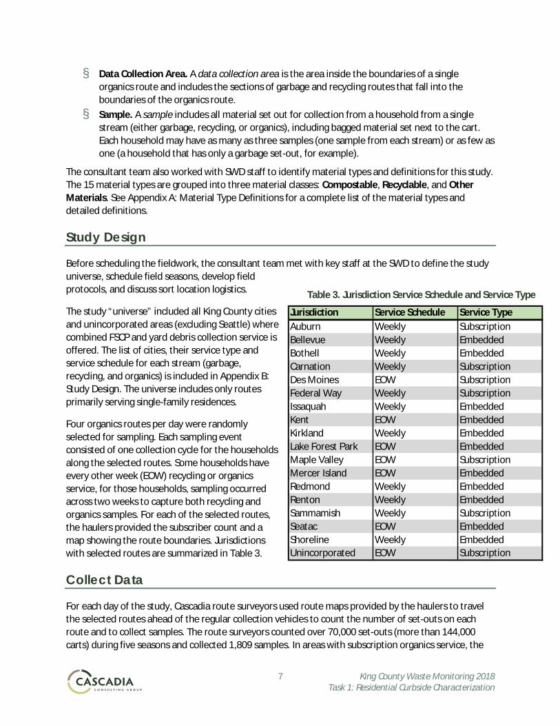
Four organics routes per day were randomly selected for sampling. Each sampling event consisted of one collection cycle for the households along the selected routes. Some households have every other week (EOW) recycling or organics service, for those households, sampling occurred across two weeks to capture both recycling and organics samples. For each of the selected routes, the haulers provided the subscriber count and a map showing the route boundaries. Jurisdictions with selected routes are summarized in Table 3.
Collect Data
For each day of the study, Cascadia route surveyors used route maps provided by the haulers to travel the selected routes ahead of the regular collection vehicles to count the number of set-outs on each route and to collect samples. The route surveyors counted over 70,000 set-outs (more than 144,000 carts) during five seasons and collected 1,809 samples. In areas with subscription organics service, the
Table 3. Jurisdiction Service Schedule and Service Type
Jurisdiction Service Schedule Service TypeAuburn Weekly SubscriptionBellevue Weekly EmbeddedBothell Weekly EmbeddedCarnation Weekly SubscriptionDes Moines EOW SubscriptionFederal Way Weekly SubscriptionIssaquah Weekly EmbeddedKent EOW EmbeddedKirkland Weekly EmbeddedLake Forest Park EOW EmbeddedMaple Valley EOW SubscriptionMercer Island EOW EmbeddedRedmond Weekly EmbeddedRenton Weekly EmbeddedSammamish Weekly SubscriptionSeatac EOW EmbeddedShoreline Weekly EmbeddedUnincorporated EOW Subscription
8 King County Waste Monitoring 2018 Task 1: Residential Curbside Characterization
route surveyors also counted the total number of households on the route where the hauler could not provide a household count. After traveling each route, the route surveyors brought the collected samples to the Bow Lake transfer station for hand sorting.
The average garbage set-out weighed approximately 23 pounds, the average recycling set-out weighed approximately 23 pounds, and the average organics set-out weighed approximately 56 pounds. The field crew sorted each sample into 15 material types; each material type was weighed independently. The crew leader recorded the weight for each sorted material type on the sampling form, reviewed the form, and later entered the data into a custom database for analysis. A full description of the hand-sort procedure is included in Appendix B: Study Design.
Changes to the Methodology from the Previous Study
By design, the current study collected and characterized organics samples in much the same way as previous studies, allowing for comparisons over time. However, this study included samples from more streams (garbage and recycling), included more field days, and simplified the material list. These bullets detail the key differences between the 2014 and 2017 studies.
§ In 2014, sampling was completed over eight field periods of two days each for 16 sampling days. In 2017, the sampling was completed over five field periods each lasting a full collection cycle (one week for most households, two weeks for some households). Collecting samples for the full collection cycle was required to sample all streams from a household with EOW service.
§ The 2014 study only collected organics samples from selected households. The current study collected samples of garbage and recycling (when set out) from the selected households in addition to the organics set-out. Including the garbage and recycling streams paints a fuller picture of the average household composition and allows for unique insights into residential solid waste patterns.
§ The material list for 2017 was streamlined to better align with SWD’s other data collection efforts and materials management initiatives.
9 King County Waste Monitoring 2018 Task 1: Residential Curbside Characterization
3. Findings
Interpreting the Composition Results
How Data Is Presented For each stream, composition data are presented in three ways throughout this report:
1. An overview of composition, by Material Class, is presented as a bar chart.
2. A table lists the five most prevalent material types. 3. A detailed table lists the full composition and quantity results
for the 15 material types. Please refer to Appendix A: Material Type Definitions for a detailed list of definitions for material types used in the study.
Throughout the report, there are also tables and figures that communicate information about participation rates, material capture rates, and the distribution of certain behaviors among households.
Means and Error Ranges The data from the sorting process were treated with a statistical procedure that provides two kinds of composition information for each of the material types:
§ Estimates of composition by weight. § The precision of the composition estimates.
All estimates of precision were calculated at the 90% confidence level. The equations used in these calculations appear in Appendix D: Calculations.
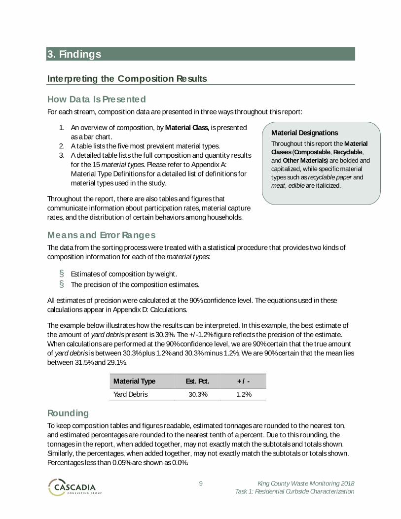
The example below illustrates how the results can be interpreted. In this example, the best estimate of the amount of yard debris present is 30.3%. The +/-1.2% figure reflects the precision of the estimate. When calculations are performed at the 90% confidence level, we are 90% certain that the true amount of yard debris is between 30.3% plus 1.2% and 30.3% minus 1.2%. We are 90% certain that the mean lies between 31.5% and 29.1%.
Material Type Est. Pct. + / -
Yard Debris 30.3% 1.2%
Rounding To keep composition tables and figures readable, estimated tonnages are rounded to the nearest ton, and estimated percentages are rounded to the nearest tenth of a percent. Due to this rounding, the tonnages in the report, when added together, may not exactly match the subtotals and totals shown. Similarly, the percentages, when added together, may not exactly match the subtotals or totals shown. Percentages less than 0.05% are shown as 0.0%.
Material Designations Throughout this report the Material Classes (Compostable, Recyclable, and Other Materials) are bolded and capitalized, while specific material types such as recyclable paper and meat, edible are italicized.
10 King County Waste Monitoring 2018 Task 1: Residential Curbside Characterization
It is important to recognize that the tons in the report were calculated using the more precise (not rounded) percentages. Using the rounded percentages to calculate tonnages yields quantities that differ from the rounded numbers in the report.
For example, the rounded percentage for yard debris in the organics stream in Table 5 is shown as 84.5%, while the more precise number, 84.4860987507027%, was used in calculations. If the rounded numbers (84.5%) had been used in the calculations, yard debris would be 143,770 tons. Using the more precise numbers, yard debris is calculated to be 143,746 tons as shown in Table 5—a difference of 24 tons.
Results
This section describes the single-family residential curbside characterization results in nine subsections:
1. Composition of single-family generation. 2. Composition of material set out in garbage service carts. 3. Composition of material set out in recycling service carts. 4. Recycling set-outs and participation rates. 5. Composition of material set out in organics service carts. 6. Organics set-outs and food scrap participation rates. 7. Capture rates for key recyclable materials. 8. Capture rates for food scrap and compostable paper. 9. Patterns of contamination behavior.
Single-family Generation
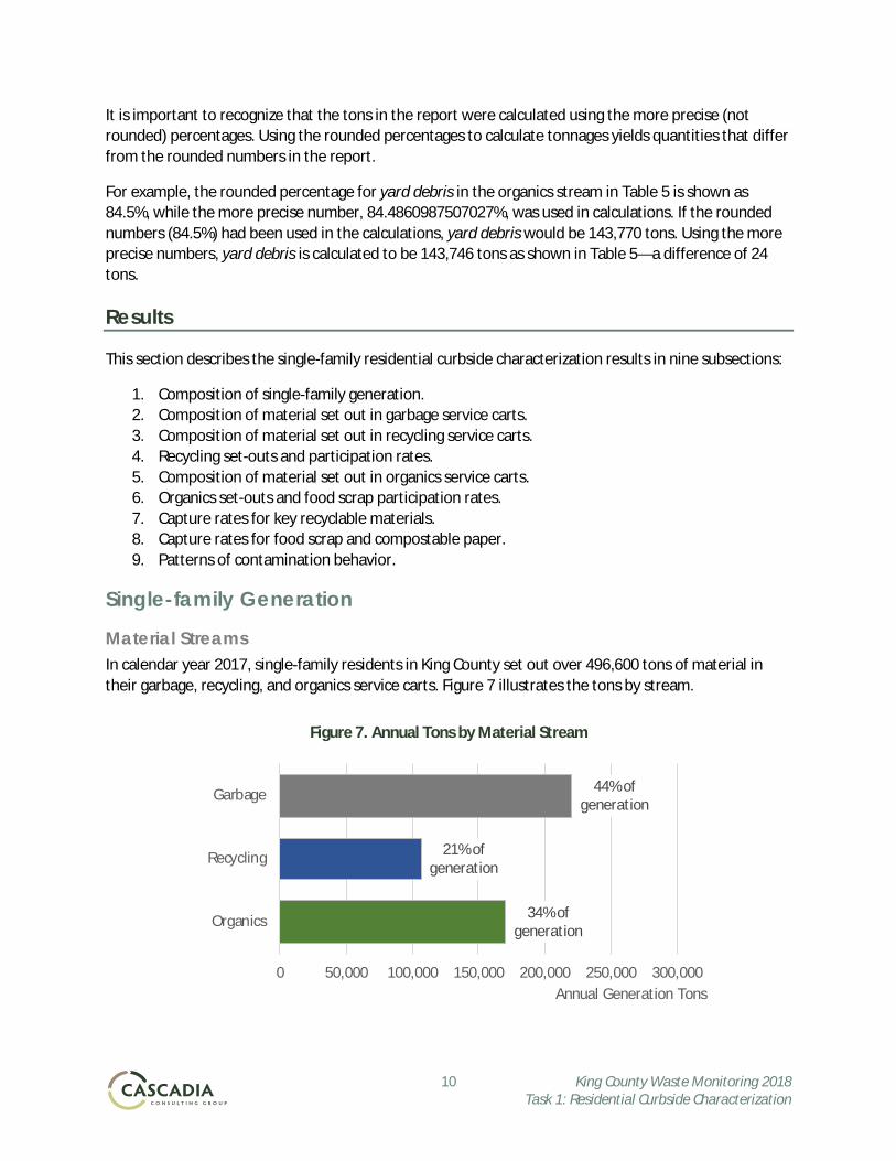
Material Streams In calendar year 2017, single-family residents in King County set out over 496,600 tons of material in their garbage, recycling, and organics service carts. Figure 7 illustrates the tons by stream.
Figure 7. Annual Tons by Material Stream
34% of generation
21% of generation
44% of generation
0 50,000 100,000 150,000 200,000 250,000 300,000
Organics
Recycling
Garbage
Annual Generation Tons

11 King County Waste Monitoring 2018 Task 1: Residential Curbside Characterization
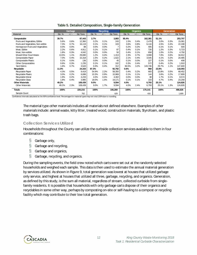
Composition Figure 8 summarizes composition by recoverability for all materials collected from single-family generators in King County. Table 4 summarizes the five most prevalent materials generated by these residents (by weight). Table 5 presents the detailed composition of materials collected from single-family generators in King County.
Key Findings
§ Of all the material generated by King County single-family households, 51% (253,707 tons) is Compostable and 24% (118,093 tons) is Recyclable.
§ The four most prevalent divertible material types (yard debris, recyclable paper, mixed/other food waste, and recyclable glass) account for over 55% of total generation.
§ Yard debris (30%, 147,600 tons) is the most prevalent material generated by single-family households in King County.
Figure 8. Composition by Material Class, Single-family Generation
Table 4. Top Five Material Types, Single-family Generation
25% of generation
24% of generation
51% of generation
0 50,000 100,000 150,000 200,000 250,000 300,000
Other Materials
Recyclable
Compostable
Annual Generation Tons
Est. Est. Material Percent Tons
Yard Debris 29.7% 147,600Other Materials 25.1% 124,826Recyclable Paper 13.8% 68,452Mixed/Other Food Waste 7.0% 34,912Recyclable Glass 4.7% 23,258
Total 80.4% 399,048
12 King County Waste Monitoring 2018 Task 1: Residential Curbside Characterization
Table 5. Detailed Composition, Single-family Generation
The material type other materials includes all materials not defined elsewhere. Examples of other materials include: animal waste, kitty litter, treated wood, construction materials, Styrofoam, and plastic trash bags.
Collection Services Utilized Households throughout the County can utilize the curbside collection services available to them in four combinations:
§ Garbage only, § Garbage and recycling, § Garbage and organics, § Garbage, recycling, and organics.
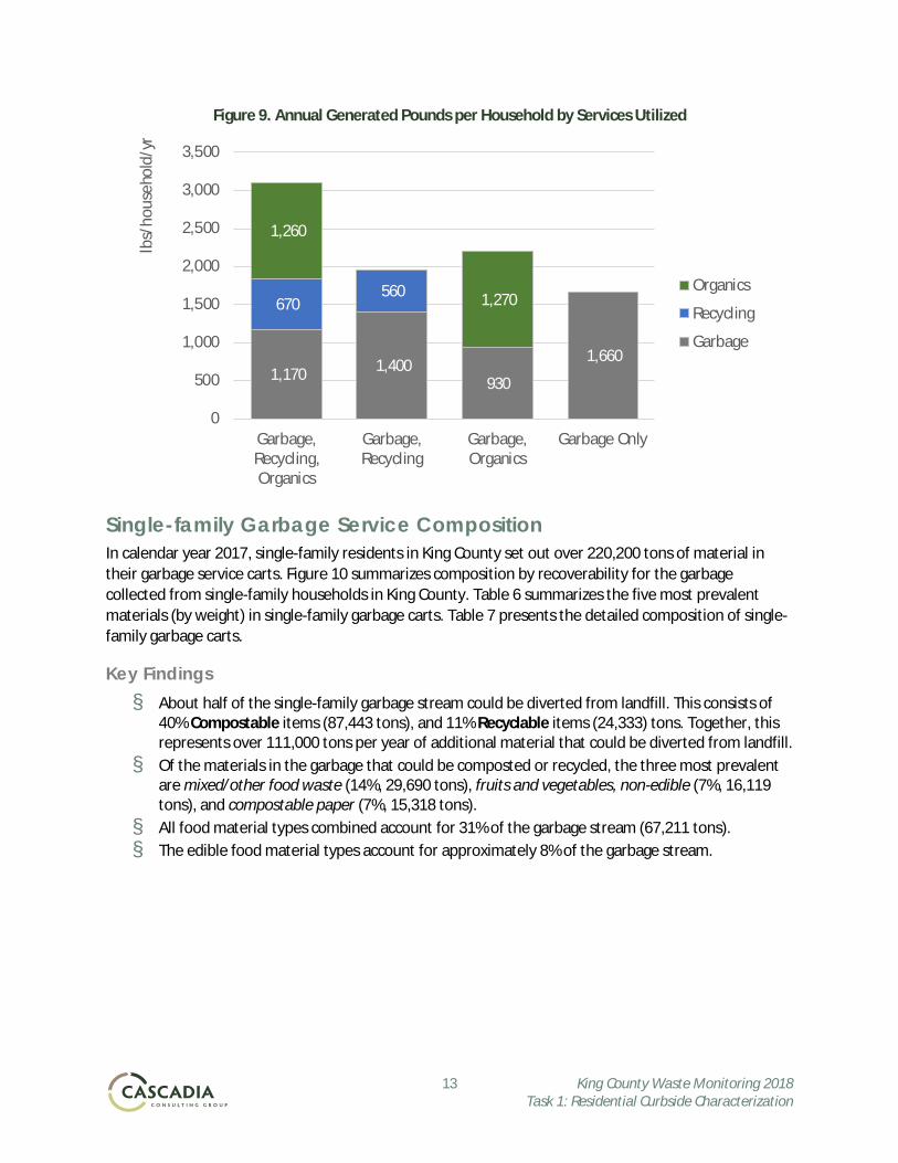
During the sampling events, the field crew noted which carts were set out at the randomly selected households and weighed each sample. This data is then used to estimate the annual material generation by services utilized. As shown in Figure 9, total generation was lowest at houses that utilized garbage only service, and highest at houses that utilized all three, garbage, recycling, and organics. Generation, as defined by this study, is the sum all material, regardless of stream, collected curbside from single-family residents. It is possible that households with only garbage carts dispose of their organics and recyclables in some other way, perhaps by composting on-site or self-hauling to a compost or recycling facility which may contribute to their low total generation.
Garbage Recycling Organics Generation Material Est. % + / - Est Tons Est. % + / - Est Tons Est. % + / - Est Tons Est. % + / - Est Tons
Compostable 39.7% 87,443 3.7% 3,883 95.4% 162,381 51.1% 253,707 Fruits and Vegetables, Edible 5.6% 0.6% 12,360 0.2% 0.1% 243 1.5% 0.4% 2,478 3.0% 0.3% 15,081 Fruits and Vegetables, Non-edible 7.3% 0.7% 16,119 0.1% 0.1% 103 3.6% 0.8% 6,116 4.5% 0.4% 22,338 Homegrown Fruits and Vegetables 0.0% 0.0% 88 0.0% 0.0% 7 0.2% 0.2% 405 0.1% 0.1% 500 Meat, Edible 2.2% 0.6% 4,911 0.1% 0.1% 87 0.4% 0.1% 726 1.2% 0.3% 5,723 Meat, Non-edible 1.8% 0.3% 4,042 0.0% 0.0% 50 0.4% 0.1% 658 1.0% 0.2% 4,750 Mixed/Other Food Waste 13.5% 1.1% 29,690 1.2% 0.4% 1,313 2.3% 0.7% 3,908 7.0% 0.6% 34,912 Compostable Paper 7.0% 0.4% 15,318 1.5% 0.2% 1,622 2.1% 0.4% 3,545 4.1% 0.2% 20,485 Compostable Plastic 0.1% 0.0% 136 0.0% 0.0% 45 0.1% 0.0% 227 0.1% 0.0% 408 Other Compostables 0.6% 0.3% 1,235 0.1% 0.1% 102 0.3% 0.4% 572 0.4% 0.2% 1,910 Yard Debris 1.6% 0.7% 3,543 0.3% 0.4% 312 84.5% 3.2% 143,746 29.7% 1.1% 147,600
Recyclable 11.0% 24,333 87.3% 92,792 0.6% 968 23.8% 118,093 Recyclable Paper 4.3% 0.5% 9,419 54.9% 2.2% 58,350 0.4% 0.2% 683 13.8% 0.5% 68,452 Recyclable Plastic 3.0% 0.2% 6,696 10.3% 0.9% 10,969 0.1% 0.1% 144 3.6% 0.2% 17,809 Recyclable Metal 1.9% 0.2% 4,233 4.0% 0.4% 4,302 0.0% 0.0% 38 1.7% 0.1% 8,574 Recyclable Glass 1.8% 0.4% 3,985 18.0% 1.5% 19,171 0.1% 0.1% 103 4.7% 0.4% 23,258
Other Materials 49.2% 108,439 9.0% 9,594 4.0% 6,793 25.1% 124,826 Other Materials 49.2% 2.3% 108,439 9.0% 1.7% 9,594 4.0% 2.4% 6,793 25.1% 1.3% 124,826
Totals 100% 220,215 100% 106,269 100% 170,141 100% 496,626Sample Count 762 629 418 1,809
Confidence intervals calculated at the 90% confidence level. Percentages for material types may not total 100% due to rounding.
13 King County Waste Monitoring 2018 Task 1: Residential Curbside Characterization
Figure 9. Annual Generated Pounds per Household by Services Utilized
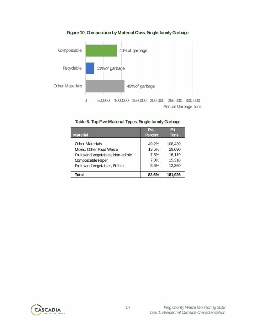
Single-family Garbage Service Composition In calendar year 2017, single-family residents in King County set out over 220,200 tons of material in their garbage service carts. Figure 10 summarizes composition by recoverability for the garbage collected from single-family households in King County. Table 6 summarizes the five most prevalent materials (by weight) in single-family garbage carts. Table 7 presents the detailed composition of single-family garbage carts.
Key Findings § About half of the single-family garbage stream could be diverted from landfill. This consists of
40% Compostable items (87,443 tons), and 11% Recyclable items (24,333) tons. Together, this represents over 111,000 tons per year of additional material that could be diverted from landfill.
§ Of the materials in the garbage that could be composted or recycled, the three most prevalent are mixed/other food waste (14%, 29,690 tons), fruits and vegetables, non-edible (7%, 16,119 tons), and compostable paper (7%, 15,318 tons).
§ All food material types combined account for 31% of the garbage stream (67,211 tons). § The edible food material types account for approximately 8% of the garbage stream.
1,170 1,400 930
1,660
670 560
1,260
1,270
0
500
1,000
1,500
2,000
2,500
3,000
3,500
Garbage,Recycling,Organics
Garbage,Recycling
Garbage,Organics
Garbage Only
lbs/
hous
ehol
d/yr
Organics
Recycling
Garbage
14 King County Waste Monitoring 2018 Task 1: Residential Curbside Characterization
Figure 10. Composition by Material Class, Single-family Garbage
Table 6. Top Five Material Types, Single-family Garbage
49% of garbage
11% of garbage
40% of garbage
0 50,000 100,000 150,000 200,000 250,000 300,000
Other Materials
Recyclable
Compostable
Annual Garbage Tons
Est. Est. Material Percent Tons
Other Materials 49.2% 108,439Mixed/Other Food Waste 13.5% 29,690Fruits and Vegetables, Non-edible 7.3% 16,119Compostable Paper 7.0% 15,318Fruits and Vegetables, Edible 5.6% 12,360
Total 82.6% 181,926
15 King County Waste Monitoring 2018 Task 1: Residential Curbside Characterization
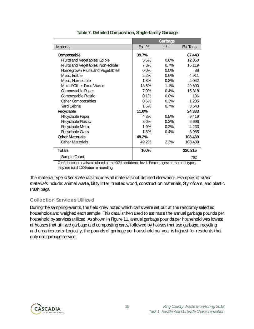
Table 7. Detailed Composition, Single-family Garbage
The material type other materials includes all materials not defined elsewhere. Examples of other materials include: animal waste, kitty litter, treated wood, construction materials, Styrofoam, and plastic trash bags.
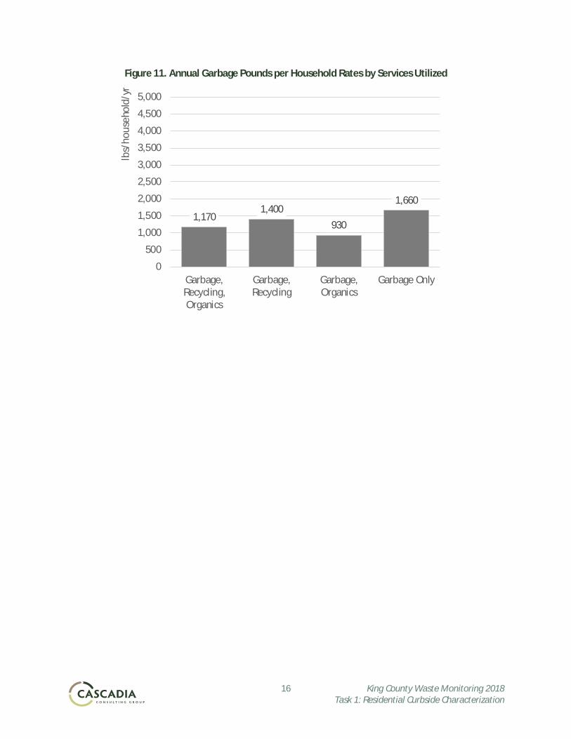
Collection Services Utilized During the sampling events, the field crew noted which carts were set out at the randomly selected households and weighed each sample. This data is then used to estimate the annual garbage pounds per household by services utilized. As shown in Figure 11, annual garbage pounds per household was lowest at houses that utilized garbage and composting carts, followed by houses that use garbage, recycling and organics carts. Logically, the pounds of garbage per household per year is highest for residents that only use garbage service.
Garbage Material Est. % + / - Est Tons
Compostable 39.7% 87,443 Fruits and Vegetables, Edible 5.6% 0.6% 12,360 Fruits and Vegetables, Non-edible 7.3% 0.7% 16,119 Homegrown Fruits and Vegetables 0.0% 0.0% 88 Meat, Edible 2.2% 0.6% 4,911 Meat, Non-edible 1.8% 0.3% 4,042 Mixed/Other Food Waste 13.5% 1.1% 29,690 Compostable Paper 7.0% 0.4% 15,318 Compostable Plastic 0.1% 0.0% 136 Other Compostables 0.6% 0.3% 1,235 Yard Debris 1.6% 0.7% 3,543
Recyclable 11.0% 24,333 Recyclable Paper 4.3% 0.5% 9,419 Recyclable Plastic 3.0% 0.2% 6,696 Recyclable Metal 1.9% 0.2% 4,233 Recyclable Glass 1.8% 0.4% 3,985
Other Materials 49.2% 108,439 Other Materials 49.2% 2.3% 108,439
Totals 100% 220,215Sample Count 762
Confidence intervals calculated at the 90% confidence level. Percentages for material types may not total 100% due to rounding.
16 King County Waste Monitoring 2018 Task 1: Residential Curbside Characterization
Figure 11. Annual Garbage Pounds per Household Rates by Services Utilized
1,170 1,400
930
1,660
0
500
1,000
1,500
2,000
2,500
3,000
3,500
4,000
4,500
5,000
Garbage,Recycling,Organics
Garbage,Recycling
Garbage,Organics
Garbage Only
lbs/
hous
ehol
d/yr
17 King County Waste Monitoring 2018 Task 1: Residential Curbside Characterization
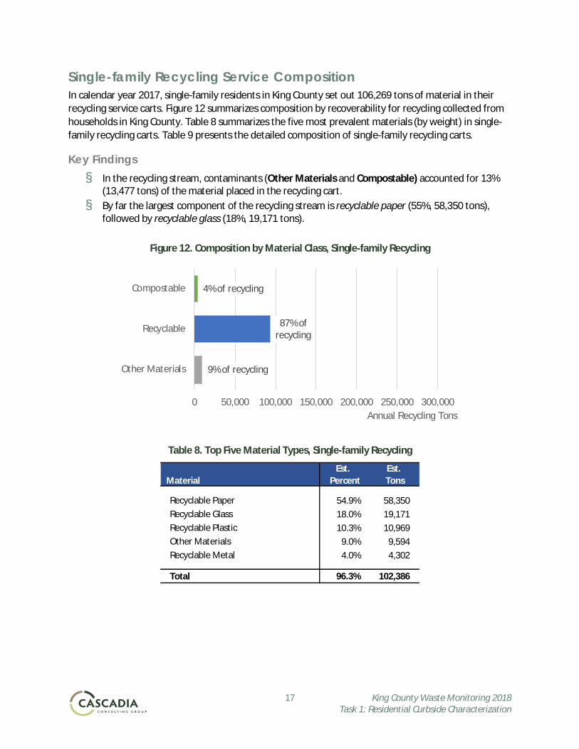
Single-family Recycling Service Composition In calendar year 2017, single-family residents in King County set out 106,269 tons of material in their recycling service carts. Figure 12 summarizes composition by recoverability for recycling collected from households in King County. Table 8 summarizes the five most prevalent materials (by weight) in single-family recycling carts. Table 9 presents the detailed composition of single-family recycling carts.
Key Findings § In the recycling stream, contaminants (Other Materials and Compostable) accounted for 13%
(13,477 tons) of the material placed in the recycling cart. § By far the largest component of the recycling stream is recyclable paper (55%, 58,350 tons),
followed by recyclable glass (18%, 19,171 tons).
Figure 12. Composition by Material Class, Single-family Recycling
Table 8. Top Five Material Types, Single-family Recycling
9% of recycling
87% of recycling
4% of recycling
0 50,000 100,000 150,000 200,000 250,000 300,000
Other Materials
Recyclable
Compostable
Annual Recycling Tons
Est. Est. Material Percent Tons
Recyclable Paper 54.9% 58,350Recyclable Glass 18.0% 19,171Recyclable Plastic 10.3% 10,969Other Materials 9.0% 9,594Recyclable Metal 4.0% 4,302
Total 96.3% 102,386
18 King County Waste Monitoring 2018 Task 1: Residential Curbside Characterization
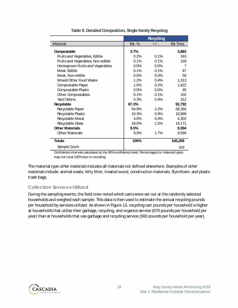
Table 9. Detailed Composition, Single-family Recycling
The material type other materials includes all materials not defined elsewhere. Examples of other materials include: animal waste, kitty litter, treated wood, construction materials, Styrofoam, and plastic trash bags.
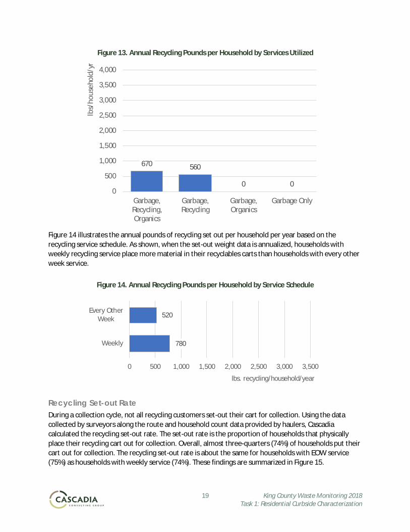
Collection Services Utilized During the sampling events, the field crew noted which carts were set out at the randomly selected households and weighed each sample. This data is then used to estimate the annual recycling pounds per household by services utilized. As shown in Figure 13, recycling cart pounds per household is higher at households that utilize their garbage, recycling, and organics service (670 pounds per household per year) than at households that use garbage and recycling service (560 pounds per household per year).
Recycling Material Est. % + / - Est Tons
Compostable 3.7% 3,883 Fruits and Vegetables, Edible 0.2% 0.1% 243 Fruits and Vegetables, Non-edible 0.1% 0.1% 103 Homegrown Fruits and Vegetables 0.0% 0.0% 7 Meat, Edible 0.1% 0.1% 87 Meat, Non-edible 0.0% 0.0% 50 Mixed/Other Food Waste 1.2% 0.4% 1,313 Compostable Paper 1.5% 0.2% 1,622 Compostable Plastic 0.0% 0.0% 45 Other Compostables 0.1% 0.1% 102 Yard Debris 0.3% 0.4% 312
Recyclable 87.3% 92,792 Recyclable Paper 54.9% 2.2% 58,350 Recyclable Plastic 10.3% 0.9% 10,969 Recyclable Metal 4.0% 0.4% 4,302 Recyclable Glass 18.0% 1.5% 19,171
Other Materials 9.0% 9,594 Other Materials 9.0% 1.7% 9,594
Totals 100% 106,269Sample Count 629
Confidence intervals calculated at the 90% confidence level. Percentages for material types may not total 100% due to rounding.
19 King County Waste Monitoring 2018 Task 1: Residential Curbside Characterization
Figure 13. Annual Recycling Pounds per Household by Services Utilized
Figure 14 illustrates the annual pounds of recycling set out per household per year based on the recycling service schedule. As shown, when the set-out weight data is annualized, households with weekly recycling service place more material in their recyclables carts than households with every other week service.
Figure 14. Annual Recycling Pounds per Household by Service Schedule
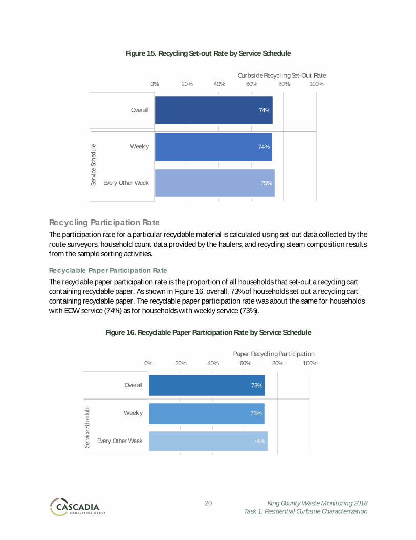
Recycling Set-out Rate During a collection cycle, not all recycling customers set-out their cart for collection. Using the data collected by surveyors along the route and household count data provided by haulers, Cascadia calculated the recycling set-out rate. The set-out rate is the proportion of households that physically place their recycling cart out for collection. Overall, almost three-quarters (74%) of households put their cart out for collection. The recycling set-out rate is about the same for households with EOW service (75%) as households with weekly service (74%). These findings are summarized in Figure 15.
670 560
0 0 0
500
1,000
1,500
2,000
2,500
3,000
3,500
4,000
Garbage,Recycling,Organics
Garbage,Recycling
Garbage,Organics
Garbage Only
lbs/
hous
ehol
d/yr
780
520
0 500 1,000 1,500 2,000 2,500 3,000 3,500
Weekly
Every OtherWeek
lbs. recycling/household/year
20 King County Waste Monitoring 2018 Task 1: Residential Curbside Characterization
Figure 15. Recycling Set-out Rate by Service Schedule
Recycling Participation Rate The participation rate for a particular recyclable material is calculated using set-out data collected by the route surveyors, household count data provided by the haulers, and recycling steam composition results from the sample sorting activities.
Recyclable Paper Participation Rate The recyclable paper participation rate is the proportion of all households that set-out a recycling cart containing recyclable paper. As shown in Figure 16, overall, 73% of households set out a recycling cart containing recyclable paper. The recyclable paper participation rate was about the same for households with EOW service (74%) as for households with weekly service (73%).
Figure 16. Recyclable Paper Participation Rate by Service Schedule
74%
74%
75%
0% 20% 40% 60% 80% 100%
Overall
Weekly
Every Other WeekServ
ice
Sche
dule
Curbside Recycling Set-Out Rate
73%
73%
74%
0% 20% 40% 60% 80% 100%
Overall
Weekly
Every Other Week
Serv
ice
Sche
dule
Paper Recycling Participation
21 King County Waste Monitoring 2018 Task 1: Residential Curbside Characterization
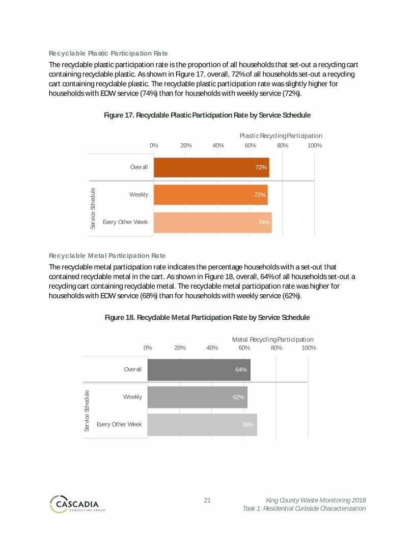
Recyclable Plastic Participation Rate The recyclable plastic participation rate is the proportion of all households that set-out a recycling cart containing recyclable plastic. As shown in Figure 17, overall, 72% of all households set-out a recycling cart containing recyclable plastic. The recyclable plastic participation rate was slightly higher for households with EOW service (74%) than for households with weekly service (72%).
Figure 17. Recyclable Plastic Participation Rate by Service Schedule
Recyclable Metal Participation Rate The recyclable metal participation rate indicates the percentage households with a set-out that contained recyclable metal in the cart. As shown in Figure 18, overall, 64% of all households set-out a recycling cart containing recyclable metal. The recyclable metal participation rate was higher for households with EOW service (68%) than for households with weekly service (62%).
Figure 18. Recyclable Metal Participation Rate by Service Schedule
72%
72%
74%
0% 20% 40% 60% 80% 100%
Overall
Weekly
Every Other Week
Serv
ice
Sche
dule
Plastic Recycling Participation
64%
62%
68%
0% 20% 40% 60% 80% 100%
Overall
Weekly
Every Other Week
Serv
ice
Sche
dule
Metal Recycling Participation
22 King County Waste Monitoring 2018 Task 1: Residential Curbside Characterization
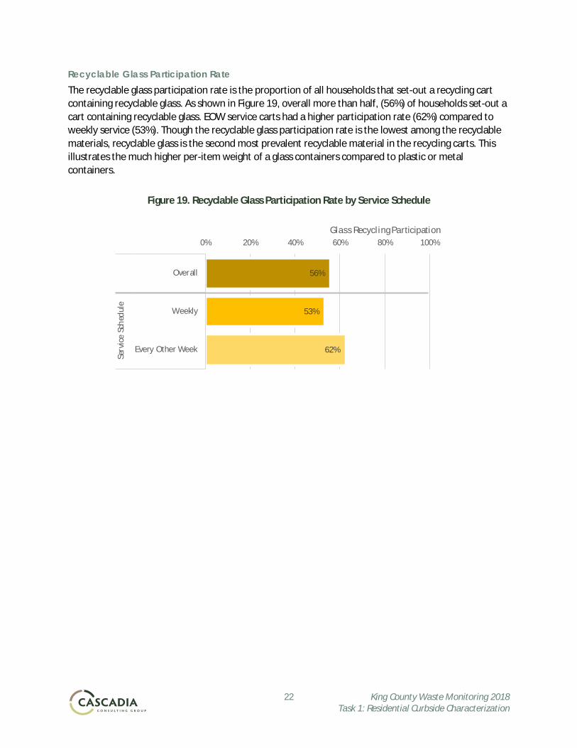
Recyclable Glass Participation Rate The recyclable glass participation rate is the proportion of all households that set-out a recycling cart containing recyclable glass. As shown in Figure 19, overall more than half, (56%) of households set-out a cart containing recyclable glass. EOW service carts had a higher participation rate (62%) compared to weekly service (53%). Though the recyclable glass participation rate is the lowest among the recyclable materials, recyclable glass is the second most prevalent recyclable material in the recycling carts. This illustrates the much higher per-item weight of a glass containers compared to plastic or metal containers.
Figure 19. Recyclable Glass Participation Rate by Service Schedule
56%
53%
62%
0% 20% 40% 60% 80% 100%
Overall
Weekly
Every Other Week
Serv
ice
Sche
dule
Glass Recycling Participation
23 King County Waste Monitoring 2018 Task 1: Residential Curbside Characterization
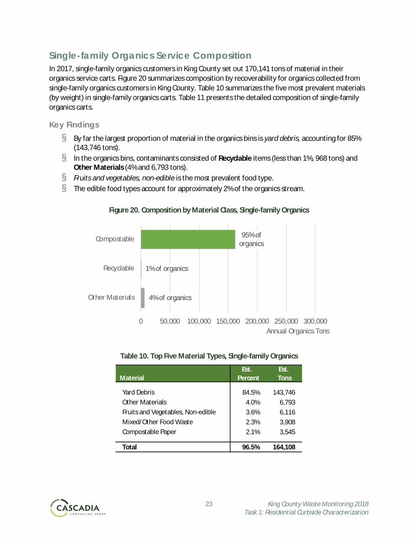
Single-family Organics Service Composition In 2017, single-family organics customers in King County set out 170,141 tons of material in their organics service carts. Figure 20 summarizes composition by recoverability for organics collected from single-family organics customers in King County. Table 10 summarizes the five most prevalent materials (by weight) in single-family organics carts. Table 11 presents the detailed composition of single-family organics carts.
Key Findings § By far the largest proportion of material in the organics bins is yard debris, accounting for 85%
(143,746 tons). § In the organics bins, contaminants consisted of Recyclable items (less than 1%, 968 tons) and
Other Materials (4% and 6,793 tons). § Fruits and vegetables, non-edible is the most prevalent food type. § The edible food types account for approximately 2% of the organics stream.
Figure 20. Composition by Material Class, Single-family Organics
Table 10. Top Five Material Types, Single-family Organics
4% of organics
1% of organics
95% of organics
0 50,000 100,000 150,000 200,000 250,000 300,000
Other Materials
Recyclable
Compostable
Annual Organics Tons
Est. Est. Material Percent Tons
Yard Debris 84.5% 143,746Other Materials 4.0% 6,793Fruits and Vegetables, Non-edible 3.6% 6,116Mixed/Other Food Waste 2.3% 3,908Compostable Paper 2.1% 3,545
Total 96.5% 164,108
24 King County Waste Monitoring 2018 Task 1: Residential Curbside Characterization
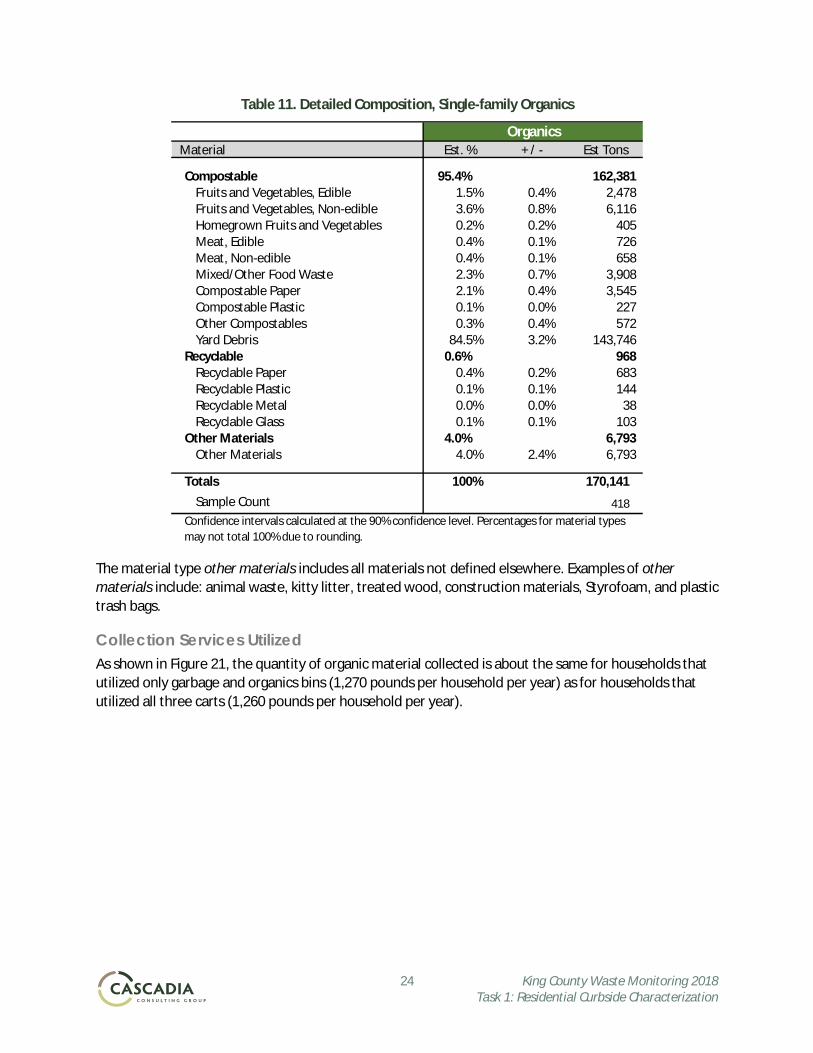
Table 11. Detailed Composition, Single-family Organics
The material type other materials includes all materials not defined elsewhere. Examples of other materials include: animal waste, kitty litter, treated wood, construction materials, Styrofoam, and plastic trash bags.
Collection Services Utilized As shown in Figure 21, the quantity of organic material collected is about the same for households that utilized only garbage and organics bins (1,270 pounds per household per year) as for households that utilized all three carts (1,260 pounds per household per year).
Organics Material Est. % + / - Est Tons
Compostable 95.4% 162,381 Fruits and Vegetables, Edible 1.5% 0.4% 2,478 Fruits and Vegetables, Non-edible 3.6% 0.8% 6,116 Homegrown Fruits and Vegetables 0.2% 0.2% 405 Meat, Edible 0.4% 0.1% 726 Meat, Non-edible 0.4% 0.1% 658 Mixed/Other Food Waste 2.3% 0.7% 3,908 Compostable Paper 2.1% 0.4% 3,545 Compostable Plastic 0.1% 0.0% 227 Other Compostables 0.3% 0.4% 572 Yard Debris 84.5% 3.2% 143,746
Recyclable 0.6% 968 Recyclable Paper 0.4% 0.2% 683 Recyclable Plastic 0.1% 0.1% 144 Recyclable Metal 0.0% 0.0% 38 Recyclable Glass 0.1% 0.1% 103
Other Materials 4.0% 6,793 Other Materials 4.0% 2.4% 6,793
Totals 100% 170,141Sample Count 418
Confidence intervals calculated at the 90% confidence level. Percentages for material types may not total 100% due to rounding.

25 King County Waste Monitoring 2018 Task 1: Residential Curbside Characterization
Figure 21. Annual Organics Pounds per Household by Services Utilized
Figure 22 illustrates the annual pounds of organics set out per organics customer, based on the service type and service schedule. As shown, organics customers with weekly service place more material in their organics carts (1,390 pounds per year for subscription, 1,190 pounds for embedded) than organics customers with EOW service (620 pounds per year for subscription, 1,070 pounds for embedded). Weekly service appears to encourage organics customers to set-out more material than EOW service.
Figure 22. Annual Organics Pounds per Household by Service Schedule and Service Type
1,260
0
1,270
0 0
500
1,000
1,500
2,000
2,500
3,000
3,500
4,000
4,500
5,000
Garbage,Recycling,Organics
Garbage,Recycling
Garbage,Organics
Garbage Only
lbs/
hous
ehol
d/yr
1,190
1,070
1,390
620
0 500 1,000 1,500 2,000 2,500 3,000 3,500
EmbeddedWeekly
EmbeddedEOW
SubscriptionWeekly
SubscriptionEOW
lbs. organics/household/year
26 King County Waste Monitoring 2018 Task 1: Residential Curbside Characterization
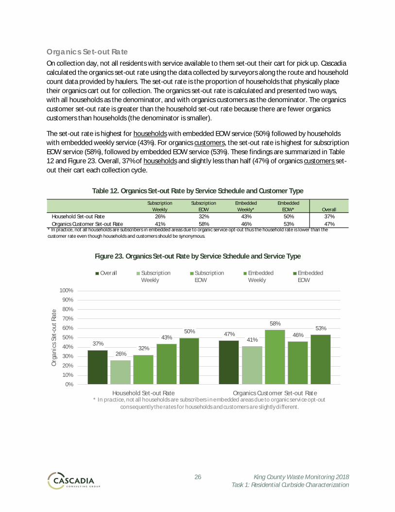
Organics Set-out Rate On collection day, not all residents with service available to them set-out their cart for pick up. Cascadia calculated the organics set-out rate using the data collected by surveyors along the route and household count data provided by haulers. The set-out rate is the proportion of households that physically place their organics cart out for collection. The organics set-out rate is calculated and presented two ways, with all households as the denominator, and with organics customers as the denominator. The organics customer set-out rate is greater than the household set-out rate because there are fewer organics customers than households (the denominator is smaller).
The set-out rate is highest for households with embedded EOW service (50%) followed by households with embedded weekly service (43%). For organics customers, the set-out rate is highest for subscription EOW service (58%), followed by embedded EOW service (53%). These findings are summarized in Table 12 and Figure 23. Overall, 37% of households and slightly less than half (47%) of organics customers set-out their cart each collection cycle.
Table 12. Organics Set-out Rate by Service Schedule and Customer Type
Figure 23. Organics Set-out Rate by Service Schedule and Service Type
Subscription Weekly
Subscription EOW
Embedded Weekly*
Embedded EOW* Overall
Household Set-out Rate 26% 32% 43% 50% 37%Organics Customer Set-out Rate 41% 58% 46% 53% 47%
* In practice, not all households are subscribers in embedded areas due to organic service opt-out thus the household rate is lower than the customer rate even though households and customers should be synonymous.
37%
47%
26%
41%32%
58%
43% 46%50% 53%
0%
10%
20%
30%
40%
50%
60%
70%
80%
90%
100%
Household Set-out Rate Organics Customer Set-out Rate
Org
anic
s Set
-out
Rat
e
Overall SubscriptionWeekly
SubscriptionEOW
EmbeddedWeekly
EmbeddedEOW
* In practice, not all households are subscribers in embedded areas due to organic service opt-out consequently the rates for households and customers are slightly di fferent.
27 King County Waste Monitoring 2018 Task 1: Residential Curbside Characterization
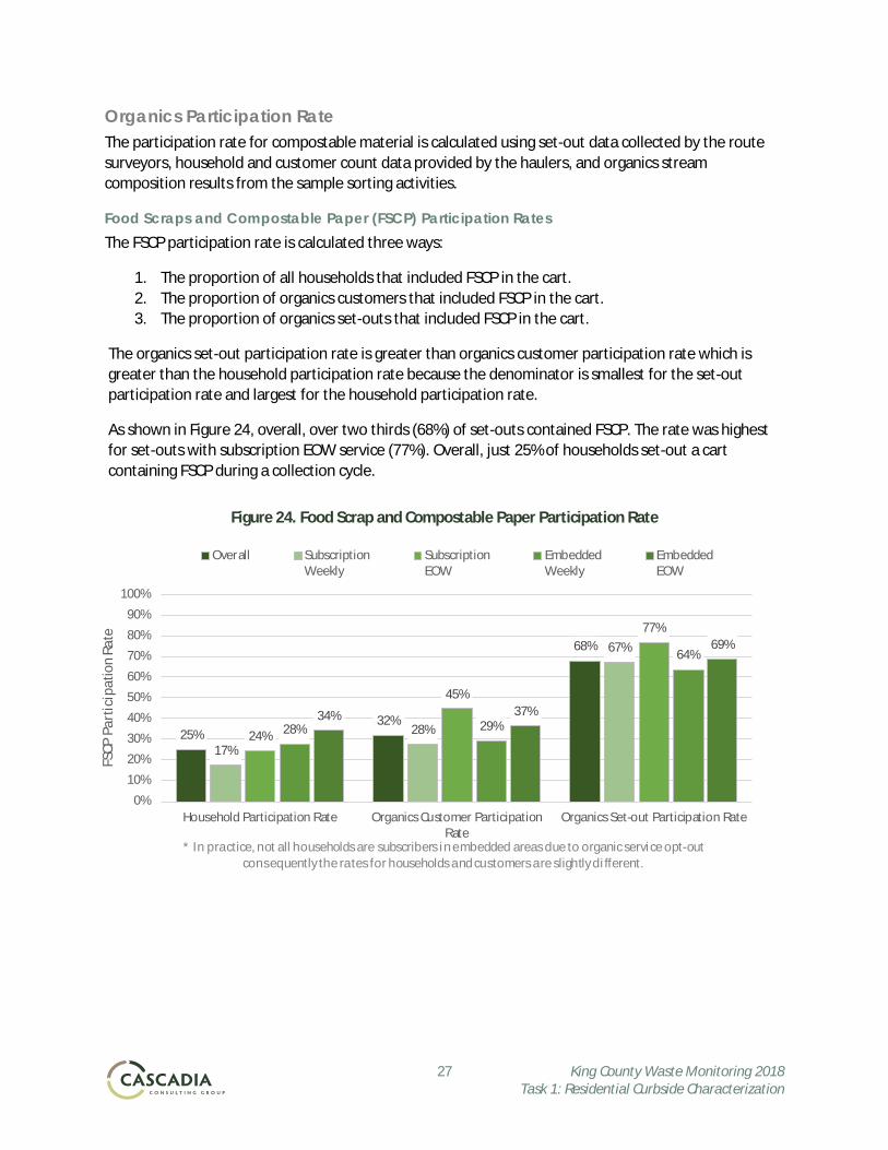
Organics Participation Rate The participation rate for compostable material is calculated using set-out data collected by the route surveyors, household and customer count data provided by the haulers, and organics stream composition results from the sample sorting activities.
Food Scraps and Compostable Paper (FSCP) Participation Rates The FSCP participation rate is calculated three ways:
1. The proportion of all households that included FSCP in the cart. 2. The proportion of organics customers that included FSCP in the cart. 3. The proportion of organics set-outs that included FSCP in the cart.
The organics set-out participation rate is greater than organics customer participation rate which is greater than the household participation rate because the denominator is smallest for the set-out participation rate and largest for the household participation rate.
As shown in Figure 24, overall, over two thirds (68%) of set-outs contained FSCP. The rate was highest for set-outs with subscription EOW service (77%). Overall, just 25% of households set-out a cart containing FSCP during a collection cycle.
Figure 24. Food Scrap and Compostable Paper Participation Rate
25%32%
68%
17%
28%
67%
24%
45%
77%
28% 29%
64%
34% 37%
69%
0%
10%
20%
30%
40%
50%
60%
70%
80%
90%
100%
Household Participation Rate Organics Customer ParticipationRate
Organics Set-out Participation Rate
FSCP
Par
ticip
atio
n Ra
te
Overall SubscriptionWeekly
SubscriptionEOW
EmbeddedWeekly
EmbeddedEOW
* In practice, not all households are subscribers in embedded areas due to organic service opt-out consequently the rates for households and customers are slightly di fferent.
28 King County Waste Monitoring 2018 Task 1: Residential Curbside Characterization
Organics Data Comparisons between Service Schedules and Subscription Types Table 13 compares key metrics between organics customer types, embedded versus subscription. The set-out rate is similar for both types of customers (48% for embedded, 46% for subscription). The FSCP participation rate is also similar for both types of customers (32% for embedded and 33% for subscription). The averaged pounds of organics per month is slightly higher for subscribers (236 pounds per month) than for those with embedded service (202 pounds per month).
Table 13. Comparison of Key Organics Metrics by Service Type
Table 14. Comparison of Key Organics Metrics by Service Type
Table 15 compares key metrics between organics collection schedules. The organics set-out rate and FSCP participation rate is highest for EOW service (55% and 39%, respectively). However, the average pounds of organics per month and averaged FSCP per month is higher for weekly service (233 and 39, respectively). This compares to 169 pounds of organics per month and 26 pounds of FSCP per month for EOW service. These data are shown in Table 16.
Table 15. Comparison of Key Organics Metrics by Service Schedule
Table 16. Comparison of Key Organics Metrics by Service Schedule
Number of Sampled Households
Organic Customers Set-out Rate
FSCP Participation Rate
Embedded 468 48% 32%Subscription 328 46% 33%Overall 796 47% 32%
Number of Organics Samples
Avg. Lbs Organics per Month*
Avg. Lbs FSCP per Month*
Embedded 277 202 40Subscription 141 236 26Overall 418 214 35
* Average for organics or FSCP participants only.
Number of Sampled Households
Organic Customers Set-out Rate
FSCP Participation Rate
Weekly 432 44% 29%EOW 364 55% 39%Overall 796 47% 32%
Number of Organics Samples
Avg. Lbs Organics per Month*
Avg. Lbs FSCP per Month*
Weekly 208 233 39EOW 210 169 26Overall 418 214 35
* Average for organics or FSCP participants only.

29 King County Waste Monitoring 2018 Task 1: Residential Curbside Characterization
Recycling Capture Rate and Diversion Efficiency Capture rate refers to the proportion (as a percentage) of a targeted material collected for diversion (recycling or composting), relative to the total quantity of that material generated. In the context of this study, it is important to note that generated is not all material created by single-family residents. In this report, the quantity generated refers to the sum of all curbside collected material: garbage, recycling, and organics. Generation does not include self-hauled materials to disposal, recycling or composting facilities, and it does not include organic material composted or otherwise managed on the residents’ property.
Even with these caveats and distinctions, capture rates are useful to help SWD staff direct education and outreach efforts where additional quantities of recyclable and compostable material could be diverted from landfill. Two main factors can increase the capture rate:
1. Increase Set-outs: It is possible to in increase the capture rate by increasing the number of recycling or organics carts set-out each collection cycle.
2. Improve Diversion Efficiency: It is possible to increase the capture rate by decreasing the amount of recoverable material a customer places in the garbage cart either by moving that material to a diversion cart or by not generating the material.
Recyclables Capture Rate As illustrated in Figure 25 the recyclables capture rate at households with weekly recycling available to them is nearly the same as at households with EOW service (79% and 78%, respectively). This appears to indicate that the service schedule does not affect whether residents place their recyclable materials in the recycling cart or garbage cart.
Figure 25. Recyclables Capture Rate by Service Schedule
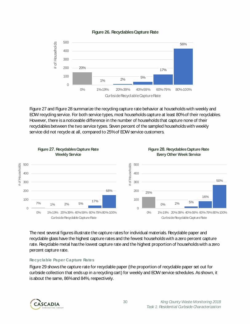
This study found that overall recyclables capture rate did not follow a normal distribution pattern throughout the population but rather a bimodal (“all or nothing”) distribution, as illustrated in the distribution of individual household capture rates in Figure 26. This figure shows the proportion of households that fall within a specified range of capture rates (each range is called a cohort). Of the households sampled for this study, the majority, 56%, place at least 80% of their recyclable materials in the recycling cart. Approximately 20% of sampled households place none of their recyclable materials in the recycling cart.
79%
79%
78%
0% 20% 40% 60% 80% 100%
Overall
Weekly
Every Other Week
Serv
ice
Sche
dule
Curbside Recycling Capture Rate
30 King County Waste Monitoring 2018 Task 1: Residential Curbside Characterization
Figure 26. Recyclables Capture Rate
Figure 27 and Figure 28 summarize the recycling capture rate behavior at households with weekly and EOW recycling service. For both service types, most households capture at least 80% of their recyclables. However, there is a noticeable difference in the number of households that capture none of their recyclables between the two service types. Seven percent of the sampled households with weekly service did not recycle at all, compared to 25% of EOW service customers.
Figure 27. Recyclables Capture Rate Weekly Service
Figure 28. Recyclables Capture Rate Every Other Week Service
The next several figures illustrate the capture rates for individual materials. Recyclable paper and recyclable glass have the highest capture rates and the fewest households with a zero percent capture rate. Recyclable metal has the lowest capture rate and the highest proportion of households with a zero percent capture rate.
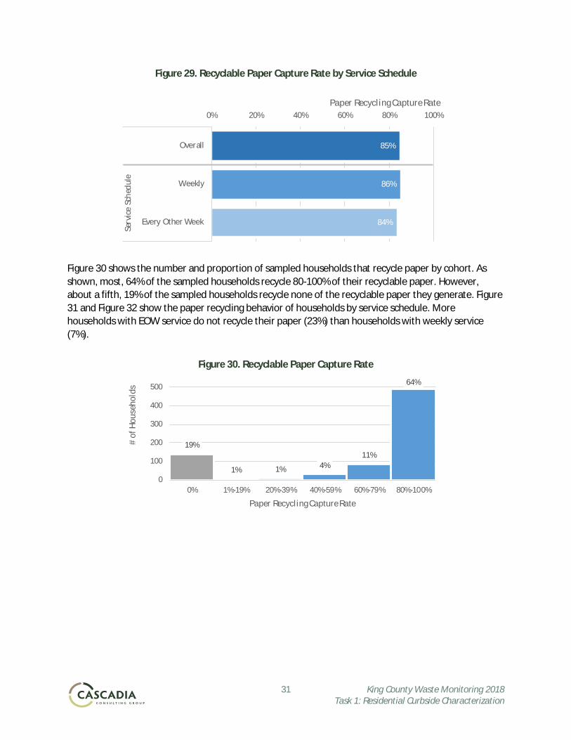
Recyclable Paper Capture Rates Figure 29 shows the capture rate for recyclable paper (the proportion of recyclable paper set out for curbside collection that ends up in a recycling cart) for weekly and EOW service schedules. As shown, it is about the same, 86% and 84%, respectively.
20%
1% 2% 5%
17%
56%
0
100
200
300
400
500
0% 1%-19% 20%-39% 40%-59% 60%-79% 80%-100%
# of
Hou
seho
lds
Curbside Recyclable Capture Rate
7% 1% 2% 5%17%
68%
0
100
200
300
400
500
0% 1%-19% 20%-39% 40%-59% 60%-79% 80%-100%
# of
Hou
seho
lds
Curbside Recyclable Capture Rate
25%
0% 2% 5%
16%
50%
0
100
200
300
400
500
0% 1%-19% 20%-39% 40%-59% 60%-79% 80%-100%
# of
Hou
seho
lds
Curbside Recyclable Capture Rate
31 King County Waste Monitoring 2018 Task 1: Residential Curbside Characterization
Figure 29. Recyclable Paper Capture Rate by Service Schedule
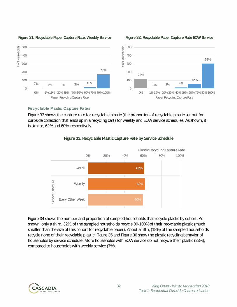
Figure 30 shows the number and proportion of sampled households that recycle paper by cohort. As shown, most, 64% of the sampled households recycle 80-100% of their recyclable paper. However, about a fifth, 19% of the sampled households recycle none of the recyclable paper they generate. Figure 31 and Figure 32 show the paper recycling behavior of households by service schedule. More households with EOW service do not recycle their paper (23%) than households with weekly service (7%).
Figure 30. Recyclable Paper Capture Rate
85%
86%
84%
0% 20% 40% 60% 80% 100%
Overall
Weekly
Every Other Week
Serv
ice
Sche
dule
Paper Recycling Capture Rate
19%
1% 1% 4%11%
64%
0
100
200
300
400
500
0% 1%-19% 20%-39% 40%-59% 60%-79% 80%-100%
# of
Hou
seho
lds
Paper Recycling Capture Rate
32 King County Waste Monitoring 2018 Task 1: Residential Curbside Characterization
Figure 31. Recyclable Paper Capture Rate, Weekly Service
Figure 32. Recyclable Paper Capture Rate EOW Service
Recyclable Plastic Capture Rates Figure 33 shows the capture rate for recyclable plastic (the proportion of recyclable plastic set out for curbside collection that ends up in a recycling cart) for weekly and EOW service schedules. As shown, it is similar, 62% and 60%, respectively.
Figure 33. Recyclable Plastic Capture Rate by Service Schedule
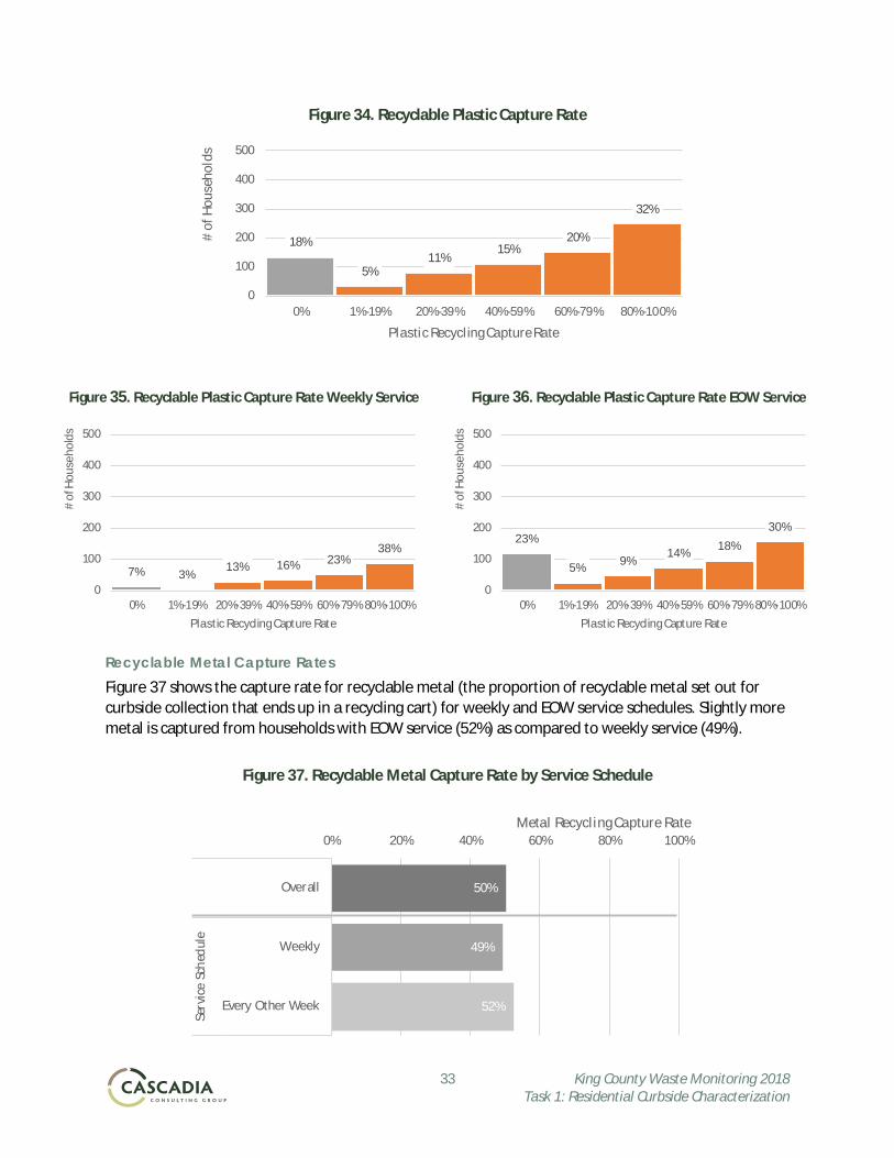
Figure 34 shows the number and proportion of sampled households that recycle plastic by cohort. As shown, only a third, 32%, of the sampled households recycle 80-100% of their recyclable plastic (much smaller than the size of this cohort for recyclable paper). About a fifth, (18%) of the sampled households recycle none of their recyclable plastic. Figure 35 and Figure 36 show the plastic recycling behavior of households by service schedule. More households with EOW service do not recycle their plastic (23%), compared to households with weekly service (7%).
7% 1% 0% 3% 10%
77%
0
100
200
300
400
500
0% 1%-19% 20%-39% 40%-59% 60%-79% 80%-100%
# of
Hou
seho
lds
Paper Recycling Capture Rate
23%
1% 2% 4%12%
59%
0
100
200
300
400
500
0% 1%-19% 20%-39% 40%-59% 60%-79% 80%-100%
# of
Hou
seho
lds
Paper Recycling Capture Rate
62%
62%
60%
0% 20% 40% 60% 80% 100%
Overall
Weekly
Every Other Week
Serv
ice
Sche
dule
Plastic Recycling Capture Rate
33 King County Waste Monitoring 2018 Task 1: Residential Curbside Characterization
Figure 34. Recyclable Plastic Capture Rate
Figure 35. Recyclable Plastic Capture Rate Weekly Service
Figure 36. Recyclable Plastic Capture Rate EOW Service
Recyclable Metal Capture Rates Figure 37 shows the capture rate for recyclable metal (the proportion of recyclable metal set out for curbside collection that ends up in a recycling cart) for weekly and EOW service schedules. Slightly more metal is captured from households with EOW service (52%) as compared to weekly service (49%).
Figure 37. Recyclable Metal Capture Rate by Service Schedule
18%
5%11%
15%20%
32%
0
100
200
300
400
500
0% 1%-19% 20%-39% 40%-59% 60%-79% 80%-100%
# of
Hou
seho
lds
Plastic Recycling Capture Rate
7% 3%13% 16% 23%
38%
0
100
200
300
400
500
0% 1%-19% 20%-39% 40%-59% 60%-79% 80%-100%
# of
Hou
seho
lds
Plastic Recycling Capture Rate
23%
5% 9%14% 18%
30%
0
100
200
300
400
500
0% 1%-19% 20%-39% 40%-59% 60%-79% 80%-100%
# of
Hou
seho
lds
Plastic Recycling Capture Rate
50%
49%
52%
0% 20% 40% 60% 80% 100%
Overall
Weekly
Every Other Week
Serv
ice
Sche
dule
Metal Recycling Capture Rate
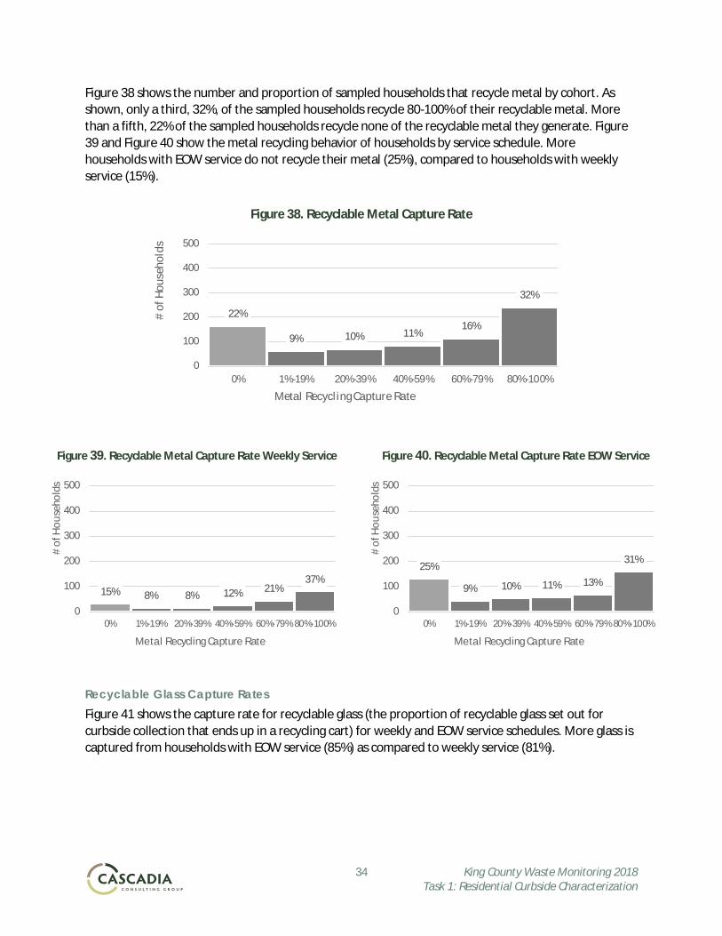
34 King County Waste Monitoring 2018 Task 1: Residential Curbside Characterization
Figure 38 shows the number and proportion of sampled households that recycle metal by cohort. As shown, only a third, 32%, of the sampled households recycle 80-100% of their recyclable metal. More than a fifth, 22% of the sampled households recycle none of the recyclable metal they generate. Figure 39 and Figure 40 show the metal recycling behavior of households by service schedule. More households with EOW service do not recycle their metal (25%), compared to households with weekly service (15%).
Figure 38. Recyclable Metal Capture Rate
Figure 39. Recyclable Metal Capture Rate Weekly Service
Figure 40. Recyclable Metal Capture Rate EOW Service
Recyclable Glass Capture Rates Figure 41 shows the capture rate for recyclable glass (the proportion of recyclable glass set out for curbside collection that ends up in a recycling cart) for weekly and EOW service schedules. More glass is captured from households with EOW service (85%) as compared to weekly service (81%).
22%
9% 10% 11%16%
32%
0
100
200
300
400
500
0% 1%-19% 20%-39% 40%-59% 60%-79% 80%-100%
# of
Hou
seho
lds
Metal Recycling Capture Rate
15% 8% 8% 12% 21%37%
0
100
200
300
400
500
0% 1%-19% 20%-39% 40%-59% 60%-79% 80%-100%
# of
Hou
seho
lds
Meta l Recycling Capture Rate
25%
9% 10% 11% 13%
31%
0
100
200
300
400
500
0% 1%-19% 20%-39% 40%-59% 60%-79% 80%-100%
# of
Hou
seho
lds
Meta l Recycling Capture Rate

35 King County Waste Monitoring 2018 Task 1: Residential Curbside Characterization
Figure 41. Recyclable Glass Capture Rate by Service Schedule
Figure 42 shows the number and proportion of sampled households that recycle glass by cohort. As shown, the majority, 72%, of the sampled households recycle 80-100% of their recyclable glass. Meanwhile, 13% of the sampled households recycle none of the recyclable glass they generate. Figure 43 and Figure 44 show the glass recycling behavior of households by service schedule. About the same proportion of households with EOW service (13%) as weekly service (11%) do not recycle their glass.
Figure 42. Recyclable Glass Capture Rate
82%
81%
85%
0% 20% 40% 60% 80% 100%
Overall
Weekly
Every Other Week
Serv
ice
Sche
dule
Glass Recycling Capture Rate
13%1% 2% 6% 6%
72%
0
100
200
300
400
500
0% 1%-19% 20%-39% 40%-59% 60%-79% 80%-100%
# of
Hou
seho
lds
Glass Recycling Capture Rate
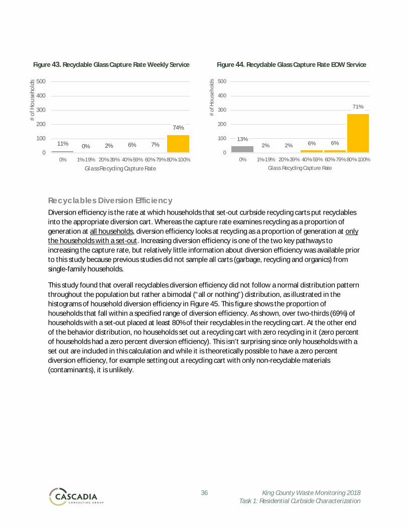
36 King County Waste Monitoring 2018 Task 1: Residential Curbside Characterization
Figure 43. Recyclable Glass Capture Rate Weekly Service
Figure 44. Recyclable Glass Capture Rate EOW Service
Recyclables Diversion Efficiency Diversion efficiency is the rate at which households that set-out curbside recycling carts put recyclables into the appropriate diversion cart. Whereas the capture rate examines recycling as a proportion of generation at all households, diversion efficiency looks at recycling as a proportion of generation at only the households with a set-out. Increasing diversion efficiency is one of the two key pathways to increasing the capture rate, but relatively little information about diversion efficiency was available prior to this study because previous studies did not sample all carts (garbage, recycling and organics) from single-family households.
This study found that overall recyclables diversion efficiency did not follow a normal distribution pattern throughout the population but rather a bimodal (“all or nothing”) distribution, as illustrated in the histograms of household diversion efficiency in Figure 45. This figure shows the proportion of households that fall within a specified range of diversion efficiency. As shown, over two-thirds (69%) of households with a set-out placed at least 80% of their recyclables in the recycling cart. At the other end of the behavior distribution, no households set out a recycling cart with zero recycling in it (zero percent of households had a zero percent diversion efficiency). This isn’t surprising since only households with a set out are included in this calculation and while it is theoretically possible to have a zero percent diversion efficiency, for example setting out a recycling cart with only non-recyclable materials (contaminants), it is unlikely.
11% 0% 2% 6% 7%
74%
0
100
200
300
400
500
0% 1%-19% 20%-39% 40%-59% 60%-79% 80%-100%
# of
Hou
seho
lds
Glass Recycling Capture Rate
13%2% 2% 6% 6%
71%
0
100
200
300
400
500
0% 1%-19% 20%-39% 40%-59% 60%-79% 80%-100%
# of
Hou
seho
lds
Glass Recycling Capture Rate
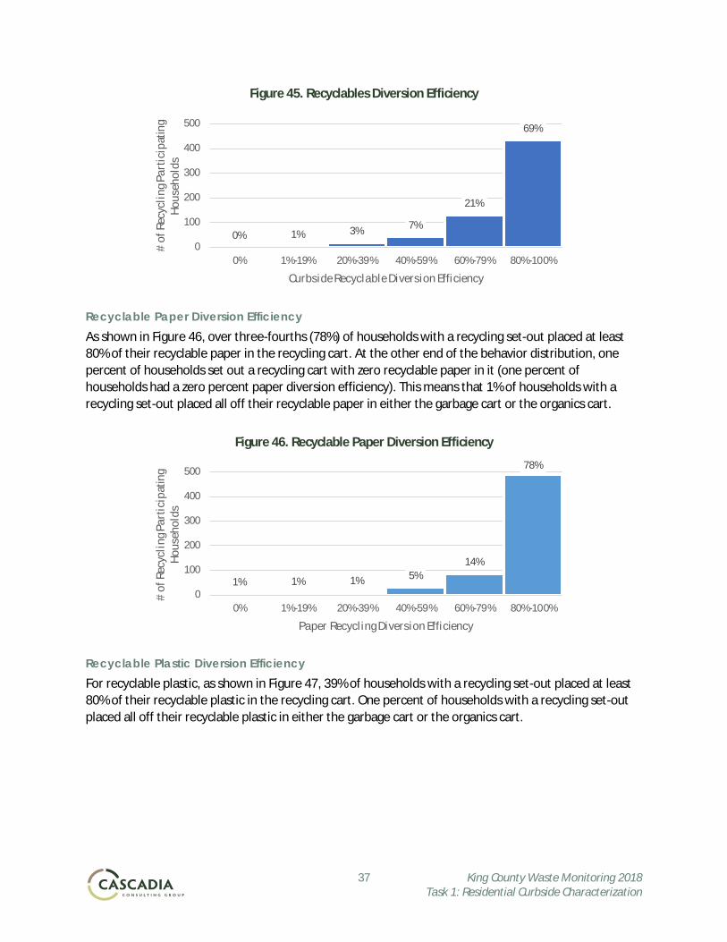
37 King County Waste Monitoring 2018 Task 1: Residential Curbside Characterization
Figure 45. Recyclables Diversion Efficiency
Recyclable Paper Diversion Efficiency As shown in Figure 46, over three-fourths (78%) of households with a recycling set-out placed at least 80% of their recyclable paper in the recycling cart. At the other end of the behavior distribution, one percent of households set out a recycling cart with zero recyclable paper in it (one percent of households had a zero percent paper diversion efficiency). This means that 1% of households with a recycling set-out placed all off their recyclable paper in either the garbage cart or the organics cart.
Figure 46. Recyclable Paper Diversion Efficiency
Recyclable Plastic Diversion Efficiency For recyclable plastic, as shown in Figure 47, 39% of households with a recycling set-out placed at least 80% of their recyclable plastic in the recycling cart. One percent of households with a recycling set-out placed all off their recyclable plastic in either the garbage cart or the organics cart.
0% 1% 3% 7%
21%
69%
0
100
200
300
400
500
0% 1%-19% 20%-39% 40%-59% 60%-79% 80%-100%
# of
Rec
yclin
g Par
ticip
atin
g Ho
useh
olds
Curbside Recyclable Diversion Efficiency
1% 1% 1% 5%14%
78%
0
100
200
300
400
500
0% 1%-19% 20%-39% 40%-59% 60%-79% 80%-100%
# of
Rec
yclin
g Par
ticip
atin
g Ho
useh
olds
Paper Recycling Diversion Efficiency

38 King County Waste Monitoring 2018 Task 1: Residential Curbside Characterization
Figure 47. Recyclable Plastic Diversion Efficiency
Recyclable Metal Diversion Efficiency As shown in Figure 48, 39% of households placed at least 80% of their recyclable metal in the recycling cart. At the other end of the behavior distribution, 7% of households with a recycling set-out placed all off their recyclable metal in either the garbage cart or the organics cart.
Figure 48. Recyclable Metal Diversion Efficiency
Recyclable Glass Diversion Efficiency Figure 49 shows the diversion efficiency for glass. As shown, over three-quarters (78%) of households with a recycling set-out placed at least 80% of their recyclable glass in the recycling cart. At the other end of the behavior distribution, 5% of households with a recycling set-out placed all their recyclable glass in either the garbage cart or the organics cart.
1%6%
13%18%
24%
39%
0
100
200
300
400
500
0% 1%-19% 20%-39% 40%-59% 60%-79% 80%-100%
# of
Rec
yclin
g Par
ticip
atin
g Ho
useh
olds
Plastic Recycling Diversion Efficiency
7% 10% 12% 14%19%
39%
0
100
200
300
400
500
0% 1%-19% 20%-39% 40%-59% 60%-79% 80%-100%
# of
Rec
yclin
g Par
ticip
atin
g Ho
useh
olds
Metal Recycling Diversion Efficiency
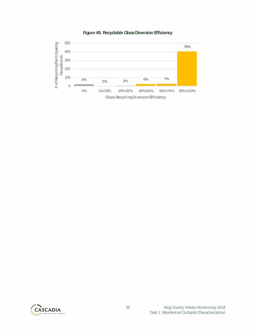
39 King County Waste Monitoring 2018 Task 1: Residential Curbside Characterization
Figure 49. Recyclable Glass Diversion Efficiency
5% 2% 2% 6% 7%
78%
0
100
200
300
400
500
0% 1%-19% 20%-39% 40%-59% 60%-79% 80%-100%
# of
Rec
yclin
g Par
ticip
atin
g Ho
useh
olds
Glass Recycling Diversion Efficiency
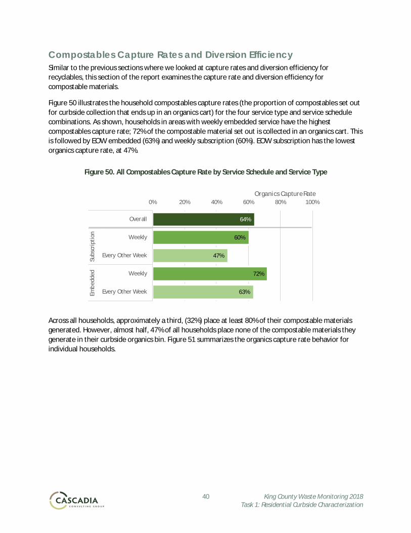
40 King County Waste Monitoring 2018 Task 1: Residential Curbside Characterization
Compostables Capture Rates and Diversion Efficiency Similar to the previous sections where we looked at capture rates and diversion efficiency for recyclables, this section of the report examines the capture rate and diversion efficiency for compostable materials.
Figure 50 illustrates the household compostables capture rates (the proportion of compostables set out for curbside collection that ends up in an organics cart) for the four service type and service schedule combinations. As shown, households in areas with weekly embedded service have the highest compostables capture rate; 72% of the compostable material set out is collected in an organics cart. This is followed by EOW embedded (63%) and weekly subscription (60%). EOW subscription has the lowest organics capture rate, at 47%.
Figure 50. All Compostables Capture Rate by Service Schedule and Service Type
Across all households, approximately a third, (32%) place at least 80% of their compostable materials generated. However, almost half, 47% of all households place none of the compostable materials they generate in their curbside organics bin. Figure 51 summarizes the organics capture rate behavior for individual households.
64%
60%
47%
72%
63%
0% 20% 40% 60% 80% 100%
Overall
Weekly
Every Other Week
Weekly
Every Other Week
Subs
crip
tion
Embe
dded
Organics Capture Rate
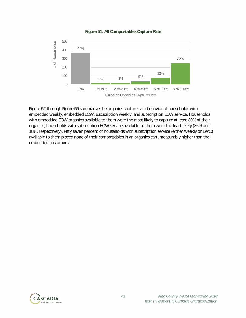
41 King County Waste Monitoring 2018 Task 1: Residential Curbside Characterization
Figure 51. All Compostables Capture Rate
Figure 52 through Figure 55 summarize the organics capture rate behavior at households with embedded weekly, embedded EOW, subscription weekly, and subscription EOW service. Households with embedded EOW organics available to them were the most likely to capture at least 80% of their organics; households with subscription EOW service available to them were the least likely (36% and 18%, respectively). Fifty seven percent of households with subscription service (either weekly or EWO) available to them placed none of their compostables in an organics cart, measurably higher than the embedded customers.
47%
2% 3% 5%10%
32%
0
100
200
300
400
500
0% 1%-19% 20%-39% 40%-59% 60%-79% 80%-100%
# of
Hou
seho
lds
Curbside Organics Capture Rate
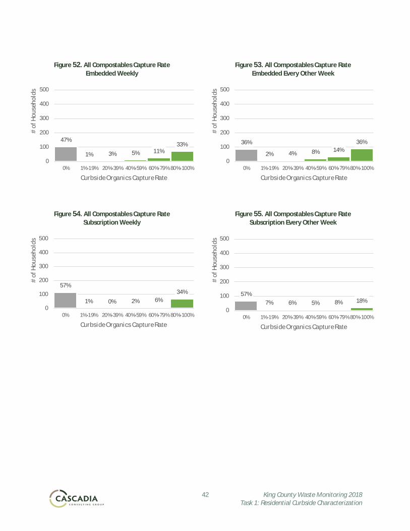
42 King County Waste Monitoring 2018 Task 1: Residential Curbside Characterization
Figure 52. All Compostables Capture Rate Embedded Weekly
Figure 53. All Compostables Capture Rate Embedded Every Other Week
Figure 54. All Compostables Capture Rate Subscription Weekly
Figure 55. All Compostables Capture Rate Subscription Every Other Week
47%
1% 3% 5% 11%33%
0
100
200
300
400
500
0% 1%-19% 20%-39% 40%-59% 60%-79% 80%-100%
# of
Hou
seho
lds
Curbside Organics Capture Rate
36%
2% 4% 8% 14%36%
0
100
200
300
400
500
0% 1%-19% 20%-39% 40%-59% 60%-79% 80%-100%
# of
Hou
seho
lds
Curbside Organics Capture Rate
57%
1% 0% 2% 6%34%
0
100
200
300
400
500
0% 1%-19% 20%-39% 40%-59% 60%-79% 80%-100%
# of
Hou
seho
lds
Curbside Organics Capture Rate
57%7% 6% 5% 8% 18%
0
100
200
300
400
500
0% 1%-19% 20%-39% 40%-59% 60%-79% 80%-100%
# of
Hou
seho
lds
Curbside Organics Capture Rate
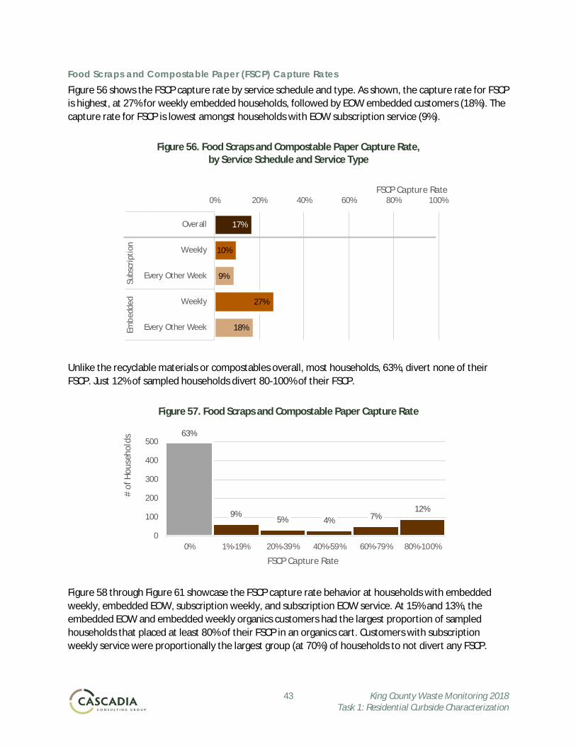
43 King County Waste Monitoring 2018 Task 1: Residential Curbside Characterization
Food Scraps and Compostable Paper (FSCP) Capture Rates Figure 56 shows the FSCP capture rate by service schedule and type. As shown, the capture rate for FSCP is highest, at 27% for weekly embedded households, followed by EOW embedded customers (18%). The capture rate for FSCP is lowest amongst households with EOW subscription service (9%).
Figure 56. Food Scraps and Compostable Paper Capture Rate, by Service Schedule and Service Type
Unlike the recyclable materials or compostables overall, most households, 63%, divert none of their FSCP. Just 12% of sampled households divert 80-100% of their FSCP.
Figure 57. Food Scraps and Compostable Paper Capture Rate
Figure 58 through Figure 61 showcase the FSCP capture rate behavior at households with embedded weekly, embedded EOW, subscription weekly, and subscription EOW service. At 15% and 13%, the embedded EOW and embedded weekly organics customers had the largest proportion of sampled households that placed at least 80% of their FSCP in an organics cart. Customers with subscription weekly service were proportionally the largest group (at 70%) of households to not divert any FSCP.
17%
10%
9%
27%
18%
0% 20% 40% 60% 80% 100%
Overall
Weekly
Every Other Week
Weekly
Every Other Week
Subs
crip
tion
Embe
dded
FSCP Capture Rate
63%
9%5% 4% 7%
12%
0
100
200
300
400
500
0% 1%-19% 20%-39% 40%-59% 60%-79% 80%-100%
# of
Hou
seho
lds
FSCP Capture Rate
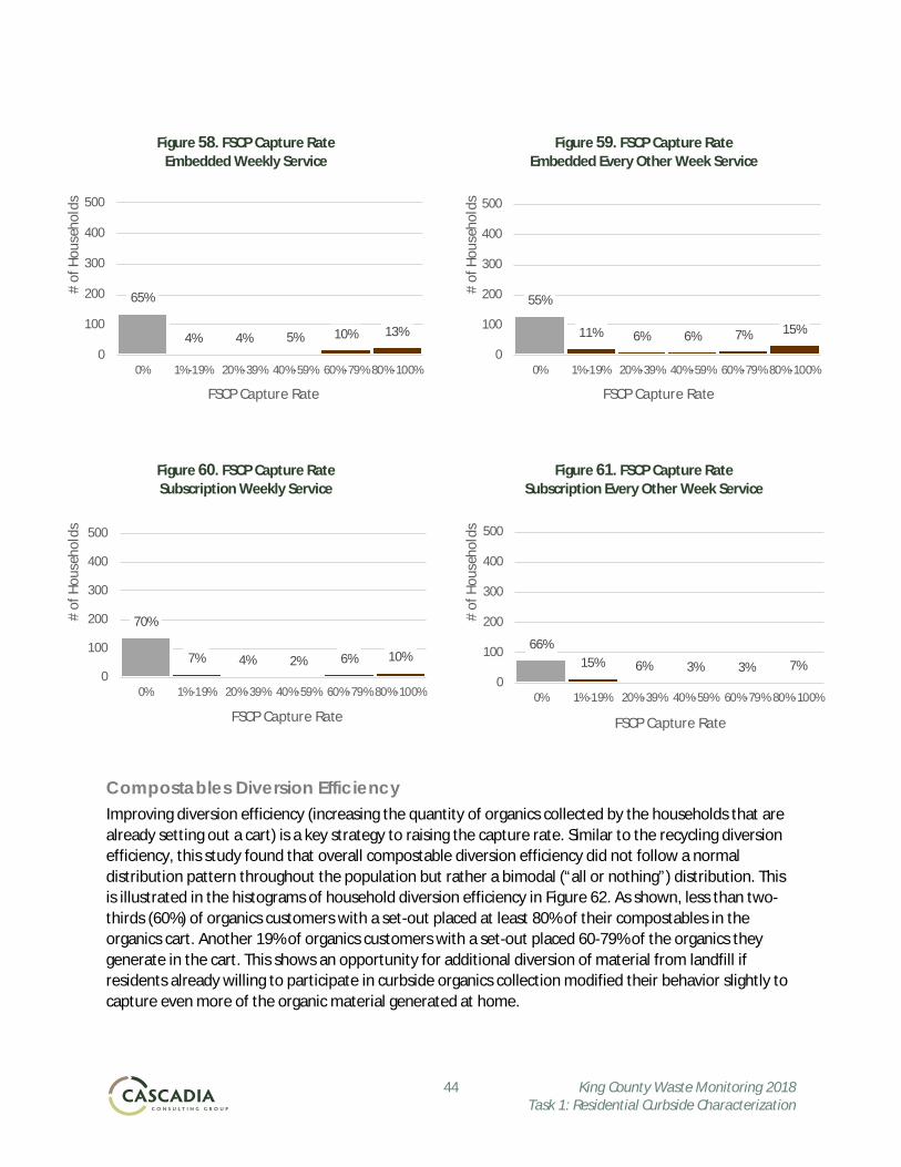
44 King County Waste Monitoring 2018 Task 1: Residential Curbside Characterization
Figure 58. FSCP Capture Rate Embedded Weekly Service
Figure 59. FSCP Capture Rate Embedded Every Other Week Service
Figure 60. FSCP Capture Rate Subscription Weekly Service
Figure 61. FSCP Capture Rate Subscription Every Other Week Service
Compostables Diversion Efficiency Improving diversion efficiency (increasing the quantity of organics collected by the households that are already setting out a cart) is a key strategy to raising the capture rate. Similar to the recycling diversion efficiency, this study found that overall compostable diversion efficiency did not follow a normal distribution pattern throughout the population but rather a bimodal (“all or nothing”) distribution. This is illustrated in the histograms of household diversion efficiency in Figure 62. As shown, less than two-thirds (60%) of organics customers with a set-out placed at least 80% of their compostables in the organics cart. Another 19% of organics customers with a set-out placed 60-79% of the organics they generate in the cart. This shows an opportunity for additional diversion of material from landfill if residents already willing to participate in curbside organics collection modified their behavior slightly to capture even more of the organic material generated at home.
65%
4% 4% 5% 10% 13%
0
100
200
300
400
500
0% 1%-19% 20%-39% 40%-59% 60%-79% 80%-100%
# of
Hou
seho
lds
FSCP Capture Rate
55%
11% 6% 6% 7% 15%
0
100
200
300
400
500
0% 1%-19% 20%-39% 40%-59% 60%-79% 80%-100%
# of
Hou
seho
lds
FSCP Capture Rate
70%
7% 4% 2% 6% 10%0
100
200
300
400
500
0% 1%-19% 20%-39% 40%-59% 60%-79% 80%-100%
# of
Hou
seho
lds
FSCP Capture Rate
66%15% 6% 3% 3% 7%
0
100
200
300
400
500
0% 1%-19% 20%-39% 40%-59% 60%-79% 80%-100%
# of
Hou
seho
lds
FSCP Capture Rate
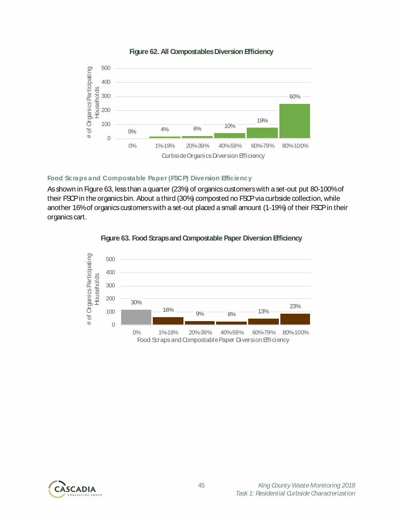
45 King County Waste Monitoring 2018 Task 1: Residential Curbside Characterization
Figure 62. All Compostables Diversion Efficiency
Food Scraps and Compostable Paper (FSCP) Diversion Efficiency As shown in Figure 63, less than a quarter (23%) of organics customers with a set-out put 80-100% of their FSCP in the organics bin. About a third (30%) composted no FSCP via curbside collection, while another 16% of organics customers with a set-out placed a small amount (1-19%) of their FSCP in their organics cart.
Figure 63. Food Scraps and Compostable Paper Diversion Efficiency
0% 4% 6% 10%19%
60%
0
100
200
300
400
500
0% 1%-19% 20%-39% 40%-59% 60%-79% 80%-100%
# of
Org
anic
s Par
ticip
atin
g Ho
useh
olds
Curbside Organics Diversion Efficiency
30%16%
9% 8% 13%23%
0
100
200
300
400
500
0% 1%-19% 20%-39% 40%-59% 60%-79% 80%-100%
# of
Org
anic
s Par
ticip
atin
g Ho
useh
olds
Food Scraps and Compostable Paper Diversion Efficiency
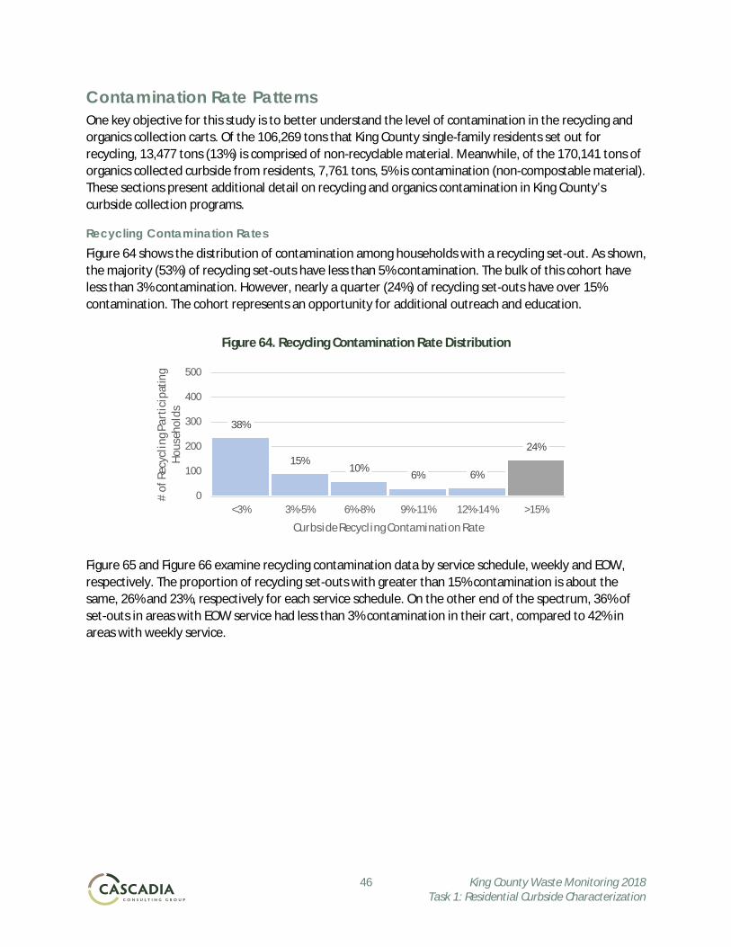
46 King County Waste Monitoring 2018 Task 1: Residential Curbside Characterization
Contamination Rate Patterns One key objective for this study is to better understand the level of contamination in the recycling and organics collection carts. Of the 106,269 tons that King County single-family residents set out for recycling, 13,477 tons (13%) is comprised of non-recyclable material. Meanwhile, of the 170,141 tons of organics collected curbside from residents, 7,761 tons, 5% is contamination (non-compostable material). These sections present additional detail on recycling and organics contamination in King County’s curbside collection programs.
Recycling Contamination Rates Figure 64 shows the distribution of contamination among households with a recycling set-out. As shown, the majority (53%) of recycling set-outs have less than 5% contamination. The bulk of this cohort have less than 3% contamination. However, nearly a quarter (24%) of recycling set-outs have over 15% contamination. The cohort represents an opportunity for additional outreach and education.
Figure 64. Recycling Contamination Rate Distribution
Figure 65 and Figure 66 examine recycling contamination data by service schedule, weekly and EOW, respectively. The proportion of recycling set-outs with greater than 15% contamination is about the same, 26% and 23%, respectively for each service schedule. On the other end of the spectrum, 36% of set-outs in areas with EOW service had less than 3% contamination in their cart, compared to 42% in areas with weekly service.
38%
15%10%
6% 6%
24%
0
100
200
300
400
500
<3% 3%-5% 6%-8% 9%-11% 12%-14% >15%
# of
Rec
yclin
g Par
ticip
atin
g Ho
useh
olds
Curbside Recycling Contamination Rate
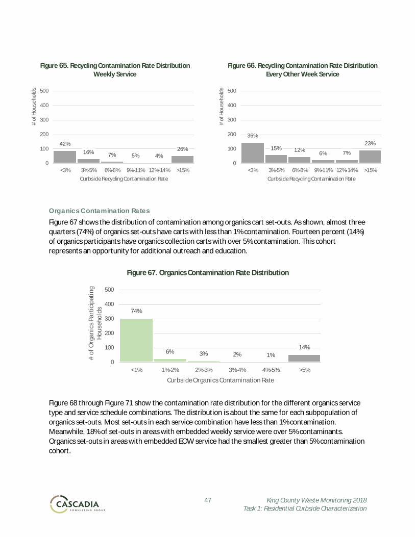
47 King County Waste Monitoring 2018 Task 1: Residential Curbside Characterization
Figure 65. Recycling Contamination Rate Distribution Weekly Service
Figure 66. Recycling Contamination Rate Distribution Every Other Week Service
Organics Contamination Rates Figure 67 shows the distribution of contamination among organics cart set-outs. As shown, almost three quarters (74%) of organics set-outs have carts with less than 1% contamination. Fourteen percent (14%) of organics participants have organics collection carts with over 5% contamination. This cohort represents an opportunity for additional outreach and education.
Figure 67. Organics Contamination Rate Distribution
Figure 68 through Figure 71 show the contamination rate distribution for the different organics service type and service schedule combinations. The distribution is about the same for each subpopulation of organics set-outs. Most set-outs in each service combination have less than 1% contamination. Meanwhile, 18% of set-outs in areas with embedded weekly service were over 5% contaminants. Organics set-outs in areas with embedded EOW service had the smallest greater than 5% contamination cohort.
42%16% 7% 5% 4%
26%
0
100
200
300
400
500
<3% 3%-5% 6%-8% 9%-11% 12%-14% >15%
# of
Hou
seho
lds
Curbside Recycling Contamination Rate
36%
15% 12% 6% 7%
23%
0
100
200
300
400
500
<3% 3%-5% 6%-8% 9%-11% 12%-14% >15%
# of
Hou
seho
lds
Curbside Recycling Contamination Rate
74%
6% 3% 2% 1%14%
0
100
200
300
400
500
<1% 1%-2% 2%-3% 3%-4% 4%-5% >5%
# of
Org
anic
s Par
ticip
atin
g Ho
useh
olds
Curbside Organics Contamination Rate
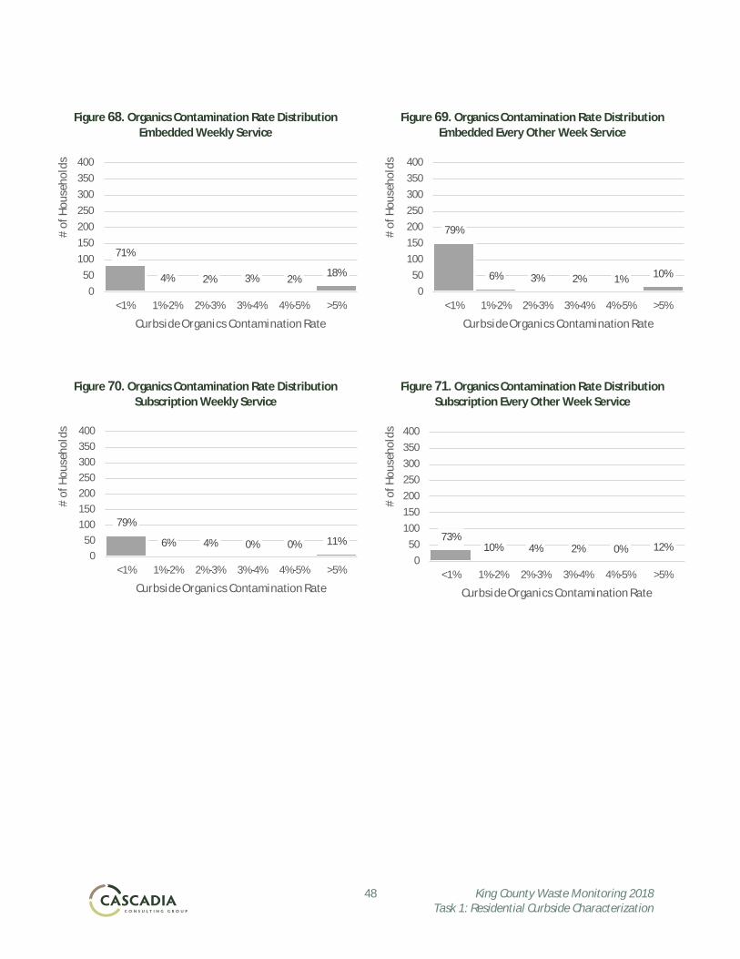
48 King County Waste Monitoring 2018 Task 1: Residential Curbside Characterization
Figure 68. Organics Contamination Rate Distribution Embedded Weekly Service
Figure 69. Organics Contamination Rate Distribution Embedded Every Other Week Service
Figure 70. Organics Contamination Rate Distribution Subscription Weekly Service
Figure 71. Organics Contamination Rate Distribution Subscription Every Other Week Service
71%
4% 2% 3% 2% 18%
050
100150200250300350400
<1% 1%-2% 2%-3% 3%-4% 4%-5% >5%
# of
Hou
seho
lds
Curbside Organics Contamination Rate
79%
6% 3% 2% 1% 10%
050
100150200250300350400
<1% 1%-2% 2%-3% 3%-4% 4%-5% >5%
# of
Hou
seho
lds
Curbside Organics Contamination Rate
79%
6% 4% 0% 0% 11%0
50100150200250300350400
<1% 1%-2% 2%-3% 3%-4% 4%-5% >5%
# of
Hou
seho
lds
Curbside Organics Contamination Rate
73%10% 4% 2% 0% 12%
050
100150200250300350400
<1% 1%-2% 2%-3% 3%-4% 4%-5% >5%
# of
Hou
seho
lds
Curbside Organics Contamination Rate
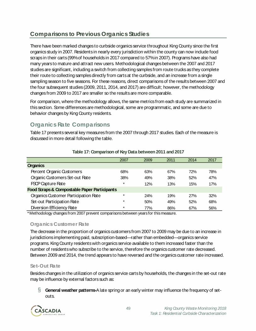
49 King County Waste Monitoring 2018 Task 1: Residential Curbside Characterization
Comparisons to Previous Organics Studies
There have been marked changes to curbside organics service throughout King County since the first organics study in 2007. Residents in nearly every jurisdiction within the county can now include food scraps in their carts (99% of households in 2017 compared to 57% in 2007). Programs have also had many years to mature and attract new users. Methodological changes between the 2007 and 2017 studies are significant, including a switch from collecting samples from route trucks as they complete their route to collecting samples directly from carts at the curbside, and an increase from a single sampling season to five seasons. For these reasons, direct comparisons of the results between 2007 and the four subsequent studies (2009, 2011, 2014, and 2017) are difficult; however, the methodology changes from 2009 to 2017 are smaller so the results are more comparable.
For comparison, where the methodology allows, the same metrics from each study are summarized in this section. Some differences are methodological, some are programmatic, and some are due to behavior changes by King County residents.
Organics Rate Comparisons Table 17 presents several key measures from the 2007 through 2017 studies. Each of the measure is discussed in more detail following the table.
Table 17: Comparison of Key Data between 2011 and 2017
Organics Customer Rate The decrease in the proportion of organics customers from 2007 to 2009 may be due to an increase in jurisdictions implementing paid, subscription-based—rather than embedded—organics service programs. King County residents with organics service available to them increased faster than the number of residents who subscribe to the service, therefore the organics customer rate decreased. Between 2009 and 2014, the trend appears to have reversed and the organics customer rate increased.
Set-Out Rate Besides changes in the utilization of organics service carts by households, the changes in the set-out rate may be influence by external factors such as:
§ General weather patterns-A late spring or an early winter may influence the frequency of set-outs.
2007 2009 2011 2014 2017Organics
Percent Organic Customers 68% 63% 67% 72% 78%Organic Customers Set-out Rate 38% 49% 38% 52% 47%FSCP Capture Rate * 12% 13% 15% 17%
Food Scraps & Compostable Paper ParticipantsOrganics Customer Participation Rate * 24% 19% 27% 32%Set-out Participation Rate * 50% 49% 52% 68%Diversion Efficiency Rate * 77% 86% 67% 56%
*Methodology changes from 2007 prevent comparisons between years for this measure.
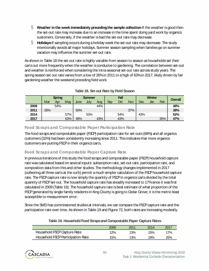
50 King County Waste Monitoring 2018 Task 1: Residential Curbside Characterization
§ Weather in the week immediately preceding the sample collection-If the weather is good then the set-out rate may increase due to an increase in the time spent doing yard work by organics customers. Conversely, if the weather is bad the set-out rate may decrease.
§ Holidays-If sampling occurs during a holiday week the set-out rate may decrease. The study intentionally avoids all major holidays. Summer season sampling when families go on summer vacation may influence the summer set-out rate.
As shown in Table 18 the set-out rate is highly variable from season to season as households set their carts out more frequently when the weather is conducive to gardening. The correlation between set-out and weather is reinforced when considering the intra-seasonal set-out rate across study years. The spring season set out rate varies from a low of 26% in 2011 to a high of 63% in 2017, likely driven by fair gardening weather the weekend preceding field work.
Table 18. Set-out Rate by Field Season
Food Scraps and Compostable Paper Participation Rate The food scraps and compostable paper (FSCP) participation rate for set-outs (68%) and all organics customers (32%) has been consistently increasing since 2011. This indicates that more organics customers are putting FSCP in their organics carts.
Food Scraps and Compostable Paper Capture Rate In previous iterations of this study the food scraps and compostable paper (FSCP) household capture rate was calculated based on several inputs: subscription rate, set-out rate, participation rate, and composition data from this and other studies. The methodology changes implemented in 2017 (collecting all three carts at the curb) permit a much simpler calculation of the FSCP household capture rate. The FSCP capture rate is now simply the quantity of FSCP in organics carts divided by the total quantity of FSCP set-out. The household capture rate has steadily increased to 17% since it was first calculated in 2009 (Table 19). The household capture rate is best estimate of what proportion of the FSCP generated by single family residents in King County is going to Cedar Grove; it is the metric least susceptible to measurement error.
Since the SWD has commissioned studies at intervals, we can compare the FSCP capture rate and the participation rate over time. As shown in Table 19 and Figure 72, both rates are increasing modestly.
Table 19. Household Food Scraps and Compostable Paper Capture Rates
Spring Summer Fall WinterMar Apr May June July Aug Sep Oct Nov Dec Jan Feb
2009 54% 44% 49%2011 26% 50% 37% 38%2014 57% 53% 54% 43% 52%2017 63% 49% 43% 43% 35% 47%
Overall
2009 2011 2014 2017Household FSCP Capture Rate 12% 13% 15% 17%Household FSCP Participation Rate 15% 13% 19% 25%
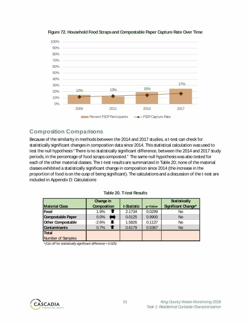
51 King County Waste Monitoring 2018 Task 1: Residential Curbside Characterization
Figure 72. Household Food Scraps and Compostable Paper Capture Rate Over Time
Composition Comparisons Because of the similarity in methods between the 2014 and 2017 studies, a t-test can check for statistically significant changes in composition data since 2014. This statistical calculation was used to test the null hypothesis “There is no statistically significant difference, between the 2014 and 2017 study periods, in the percentage of food scraps composted.” The same null hypothesis was also tested for each of the other material classes. The t-test results are summarized in Table 20; none of the material classes exhibited a statistically significant change in composition since 2014 (the increase in the proportion of food is on the cusp of being significant). The calculations and a discussion of the t-test are included in Appendix D: Calculations
Table 20. T-test Results
12% 13% 15%17%
0%
10%
20%
30%
40%
50%
60%
70%
80%
90%
100%
2009 2011 2014 2017
Percent FSCP Participants FSCP Capture Rate
Change in Material Class Composition t-Statistic p-ValueFood 1.9% 2.1734 0.0299 NoCompostable Paper 0.0% 0.0125 0.9900 NoOther Compostable -2.6% 1.5826 0.1137 NoContaminants 0.7% 0.6179 0.5367 NoTotalNumber of Samples*(Cut-off for statistically significant difference = 0.025)
Statistically Significant Change*

52 King County Waste Monitoring 2018 Task 1: Residential Curbside Characterization
Appendix A: Material Type Definitions
Compostable Items 1. Fruits and Vegetables, Edible—the edible portion of food that comes from a plant but does not
appear to have grown on the customer’s property. Examples include vegetables and fruits. Includes fruits and vegetables in the original or another container when the container weight is less than 10% of the total weight.
2. Fruits and Vegetables, Non-edible —the non-edible portions of food that comes from plants. Examples include fruit peels, vegetable peelings and potato skins, pits, cores, juiced oranges.
3. Homegrown Fruits and Vegetables—food that comes from a plant growing on or cleared from the customer’s property. Examples will include fruits and vegetables disposed of in the set-out because of falling or pruning from trees and gardens.
4. Meat, Edible—the edible portion of non-dairy food that comes from an animal. Examples include eggs and eggs in shell, fresh meat, cooked meat, and meat scraps. Does not include dairy products such as cheese and milk. Includes meat in the original or another container when the container weight is less than 10% of the total weight.
5. Meat, Non-edible —the non-edible portions of food that comes from an animal. Examples include egg shells, bones, gristle and meat trimmings, fish skins, and seafood shells.
6. Mixed/Other Food Waste—any food that cannot be put in the above categories. Examples include food items that are a combination of the above categories, as well as coffee grounds, tea packets, grains, crackers, bread, dairy, and cereal. Includes food in the original or another container when the container weight is less than 10% of the total weight.
7. Compostable Paper—any food-soiled and other compostable paper items without a plastic lining/coating, such as paper towels, napkins, tissues, uncoated paper bags and wrapping, and other papers that were soiled with food during use; uncoated paper food service packaging (e.g. cups, plates, bowls); compostable paper cups; pizza boxes; waxed cardboard boxes; coffee filters; newspaper (if used to contain food waste); and shredded paper.
8. Yard Debris—includes leaves, grass clippings, sod, garden wastes, brush, prunings, logs, and clumped soil and rocks associated with yard debris.
9. Compostable Plastic—includes compostable plastic items, such as film “plastic” bags made of materials such as corn starch or soy designed to compost (e.g. BioBag, EcoSafe) and compostable plastic (“PLA”) containers and packaging (e.g. cups/lids, bowls, clamshells, plates, trays, cutlery, straws). Compostable plastic containers and packaging are marked with the words “compostable” or “#7 PLA” in the plastic identifier.
10. Other Compostables—other compostable organic materials, not included above, such as hair, popsicle sticks, chopsticks, and toothpicks.
Recyclable Items 11. Recyclable Paper—includes non-coated paper and bleached polycoated paperboard cartons
normally recycled in curbside collection programs when not significantly contaminated. Examples include newspapers (not used to contain food waste), newspaper inserts, corrugated cardboard, magazines, phone books, junk mail, chipboard, boxboard, egg cartons, printing, writing paper, milk cartons, ice cream cartons, and paper cups with a plastic layer designed to be used for beverages or food (e.g. most to-go coffee cups and fast food soda cups).
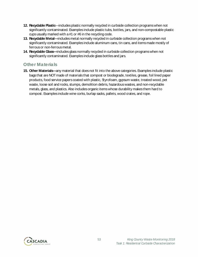
53 King County Waste Monitoring 2018 Task 1: Residential Curbside Characterization
12. Recyclable Plastic—includes plastic normally recycled in curbside collection programs when not significantly contaminated. Examples include plastic tubs, bottles, jars, and non-compostable plastic cups usually marked with a #1 or #6 in the recycling code.
13. Recyclable Metal—includes metal normally recycled in curbside collection programs when not significantly contaminated. Examples include aluminum cans, tin cans, and items made mostly of ferrous or non-ferrous metal.
14. Recyclable Glass—includes glass normally recycled in curbside collection programs when not significantly contaminated. Examples include glass bottles and jars.
Other Materials 15. Other Materials—any material that does not fit into the above categories. Examples include plastic
bags that are NOT made of materials that compost or biodegrade, textiles, grease, foil lined paper products, food service papers coated with plastic, Styrofoam, gypsum waste, treated wood, pet waste, loose soil and rocks, stumps, demolition debris, hazardous wastes, and non-recyclable metals, glass, and plastics. Also includes organic items whose durability makes them hard to compost. Examples include wine corks, burlap sacks, pallets, wood crates, and rope.
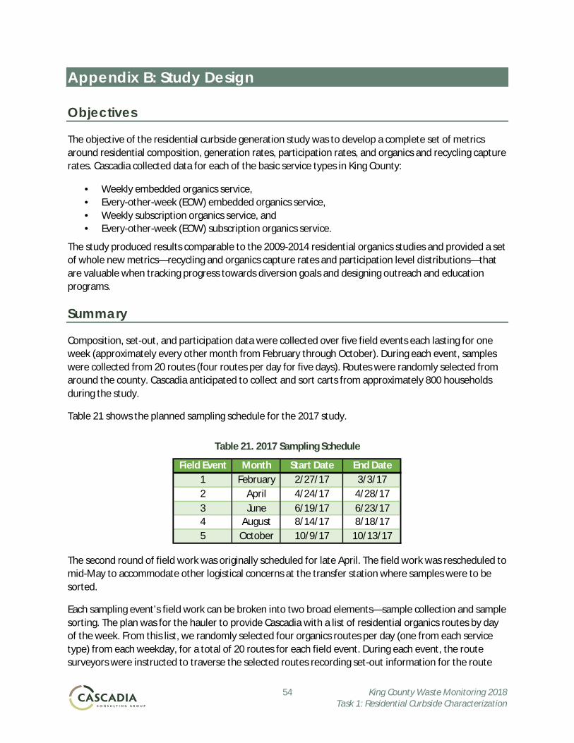
54 King County Waste Monitoring 2018 Task 1: Residential Curbside Characterization
Appendix B: Study Design
Objectives
The objective of the residential curbside generation study was to develop a complete set of metrics around residential composition, generation rates, participation rates, and organics and recycling capture rates. Cascadia collected data for each of the basic service types in King County:
· Weekly embedded organics service, · Every-other-week (EOW) embedded organics service, · Weekly subscription organics service, and · Every-other-week (EOW) subscription organics service.
The study produced results comparable to the 2009-2014 residential organics studies and provided a set of whole new metrics—recycling and organics capture rates and participation level distributions—that are valuable when tracking progress towards diversion goals and designing outreach and education programs.
Summary
Composition, set-out, and participation data were collected over five field events each lasting for one week (approximately every other month from February through October). During each event, samples were collected from 20 routes (four routes per day for five days). Routes were randomly selected from around the county. Cascadia anticipated to collect and sort carts from approximately 800 households during the study.
Table 21 shows the planned sampling schedule for the 2017 study.
Table 21. 2017 Sampling Schedule
The second round of field work was originally scheduled for late April. The field work was rescheduled to mid-May to accommodate other logistical concerns at the transfer station where samples were to be sorted.
Each sampling event’s field work can be broken into two broad elements—sample collection and sample sorting. The plan was for the hauler to provide Cascadia with a list of residential organics routes by day of the week. From this list, we randomly selected four organics routes per day (one from each service type) from each weekday, for a total of 20 routes for each field event. During each event, the route surveyors were instructed to traverse the selected routes recording set-out information for the route
Field Event Month Start Date End Date1 February 2/27/17 3/3/172 April 4/24/17 4/28/173 June 6/19/17 6/23/174 August 8/14/17 8/18/175 October 10/9/17 10/13/17
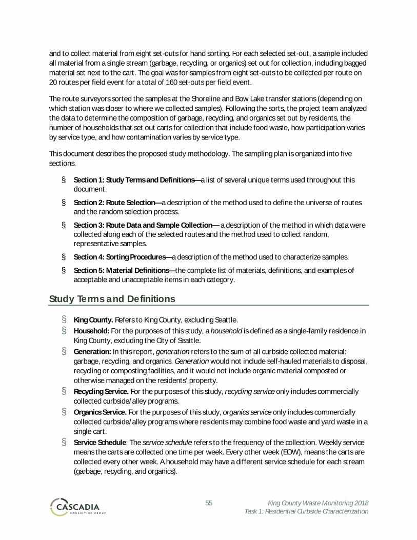
55 King County Waste Monitoring 2018 Task 1: Residential Curbside Characterization
and to collect material from eight set-outs for hand sorting. For each selected set-out, a sample included all material from a single stream (garbage, recycling, or organics) set out for collection, including bagged material set next to the cart. The goal was for samples from eight set-outs to be collected per route on 20 routes per field event for a total of 160 set-outs per field event.
The route surveyors sorted the samples at the Shoreline and Bow Lake transfer stations (depending on which station was closer to where we collected samples). Following the sorts, the project team analyzed the data to determine the composition of garbage, recycling, and organics set out by residents, the number of households that set out carts for collection that include food waste, how participation varies by service type, and how contamination varies by service type.
This document describes the proposed study methodology. The sampling plan is organized into five sections.
§ Section 1: Study Terms and Definitions—a list of several unique terms used throughout this document.
§ Section 2: Route Selection—a description of the method used to define the universe of routes and the random selection process.
§ Section 3: Route Data and Sample Collection— a description of the method in which data were collected along each of the selected routes and the method used to collect random, representative samples.
§ Section 4: Sorting Procedures—a description of the method used to characterize samples.
§ Section 5: Material Definitions—the complete list of materials, definitions, and examples of acceptable and unacceptable items in each category.
Study Terms and Definitions
§ King County. Refers to King County, excluding Seattle. § Household: For the purposes of this study, a household is defined as a single-family residence in
King County, excluding the City of Seattle. § Generation: In this report, generation refers to the sum of all curbside collected material:
garbage, recycling, and organics. Generation would not include self-hauled materials to disposal, recycling or composting facilities, and it would not include organic material composted or otherwise managed on the residents’ property.
§ Recycling Service. For the purposes of this study, recycling service only includes commercially collected curbside/alley programs.
§ Organics Service. For the purposes of this study, organics service only includes commercially collected curbside/alley programs where residents may combine food waste and yard waste in a single cart.
§ Service Schedule: The service schedule refers to the frequency of the collection. Weekly service means the carts are collected one time per week. Every other week (EOW), means the carts are collected every other week. A household may have a different service schedule for each stream (garbage, recycling, and organics).
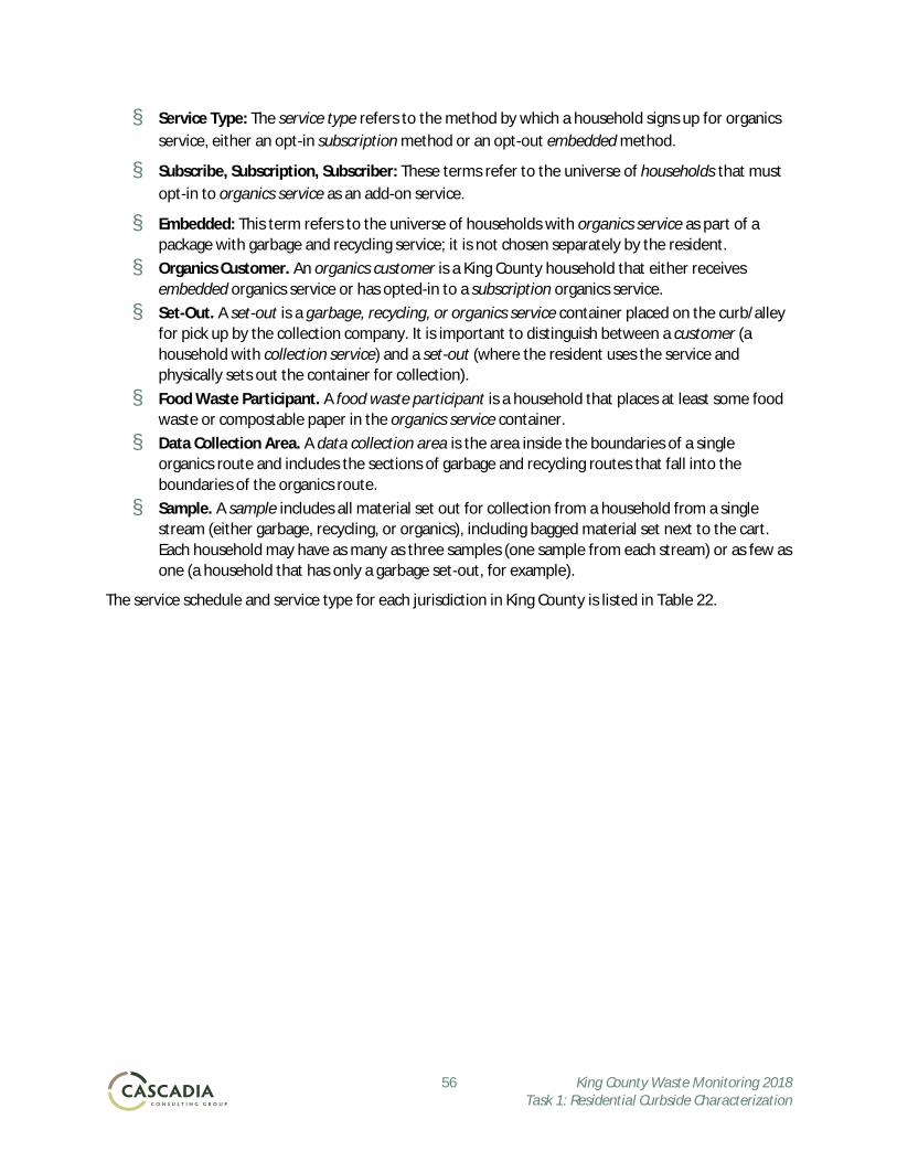
56 King County Waste Monitoring 2018 Task 1: Residential Curbside Characterization
§ Service Type: The service type refers to the method by which a household signs up for organics service, either an opt-in subscription method or an opt-out embedded method.
§ Subscribe, Subscription, Subscriber: These terms refer to the universe of households that must opt-in to organics service as an add-on service.
§ Embedded: This term refers to the universe of households with organics service as part of a package with garbage and recycling service; it is not chosen separately by the resident.
§ Organics Customer. An organics customer is a King County household that either receives embedded organics service or has opted-in to a subscription organics service.
§ Set-Out. A set-out is a garbage, recycling, or organics service container placed on the curb/alley for pick up by the collection company. It is important to distinguish between a customer (a household with collection service) and a set-out (where the resident uses the service and physically sets out the container for collection).
§ Food Waste Participant. A food waste participant is a household that places at least some food waste or compostable paper in the organics service container.
§ Data Collection Area. A data collection area is the area inside the boundaries of a single organics route and includes the sections of garbage and recycling routes that fall into the boundaries of the organics route.
§ Sample. A sample includes all material set out for collection from a household from a single stream (either garbage, recycling, or organics), including bagged material set next to the cart. Each household may have as many as three samples (one sample from each stream) or as few as one (a household that has only a garbage set-out, for example).
The service schedule and service type for each jurisdiction in King County is listed in Table 22.
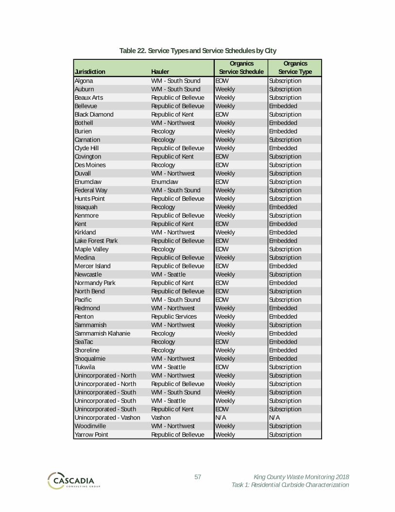
57 King County Waste Monitoring 2018 Task 1: Residential Curbside Characterization
Table 22. Service Types and Service Schedules by City
Organics OrganicsJurisdiction Hauler Service Schedule Service TypeAlgona WM - South Sound EOW SubscriptionAuburn WM - South Sound Weekly SubscriptionBeaux Arts Republic of Bellevue Weekly SubscriptionBellevue Republic of Bellevue Weekly EmbeddedBlack Diamond Republic of Kent EOW SubscriptionBothell WM - Northwest Weekly EmbeddedBurien Recology Weekly EmbeddedCarnation Recology Weekly SubscriptionClyde Hill Republic of Bellevue Weekly EmbeddedCovington Republic of Kent EOW SubscriptionDes Moines Recology EOW SubscriptionDuvall WM - Northwest Weekly SubscriptionEnumclaw Enumclaw EOW SubscriptionFederal Way WM - South Sound Weekly SubscriptionHunts Point Republic of Bellevue Weekly SubscriptionIssaquah Recology Weekly EmbeddedKenmore Republic of Bellevue Weekly SubscriptionKent Republic of Kent EOW EmbeddedKirkland WM - Northwest Weekly EmbeddedLake Forest Park Republic of Bellevue EOW EmbeddedMaple Valley Recology EOW SubscriptionMedina Republic of Bellevue Weekly SubscriptionMercer Island Republic of Bellevue EOW EmbeddedNewcastle WM - Seattle Weekly SubscriptionNormandy Park Republic of Kent EOW EmbeddedNorth Bend Republic of Bellevue EOW SubscriptionPacific WM - South Sound EOW SubscriptionRedmond WM - Northwest Weekly EmbeddedRenton Republic Services Weekly EmbeddedSammamish WM - Northwest Weekly SubscriptionSammamish Klahanie Recology Weekly EmbeddedSeaTac Recology EOW EmbeddedShoreline Recology Weekly EmbeddedSnoqualmie WM - Northwest Weekly EmbeddedTukwila WM - Seattle EOW SubscriptionUnincorporated - North WM - Northwest Weekly SubscriptionUnincorporated - North Republic of Bellevue Weekly SubscriptionUnincorporated - South WM - South Sound Weekly SubscriptionUnincorporated - South WM - Seattle Weekly SubscriptionUnincorporated - South Republic of Kent EOW SubscriptionUnincorporated - Vashon Vashon N/A N/AWoodinville WM - Northwest Weekly SubscriptionYarrow Point Republic of Bellevue Weekly Subscription
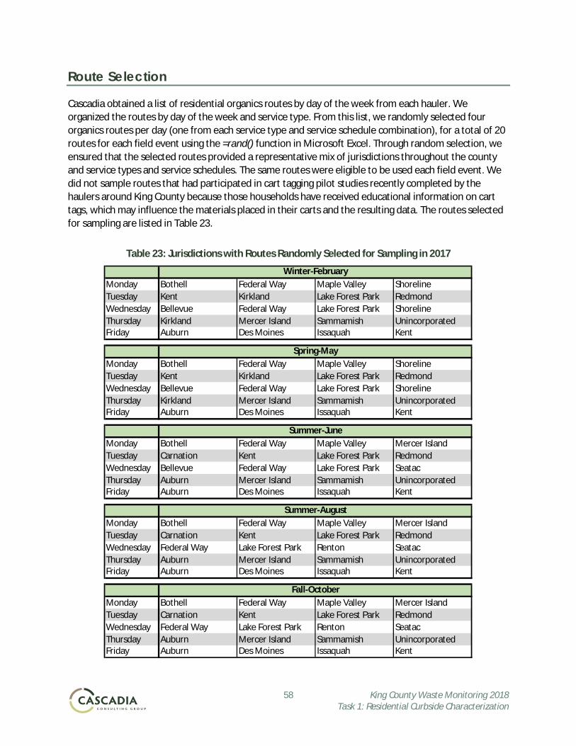
58 King County Waste Monitoring 2018 Task 1: Residential Curbside Characterization
Route Selection
Cascadia obtained a list of residential organics routes by day of the week from each hauler. We organized the routes by day of the week and service type. From this list, we randomly selected four organics routes per day (one from each service type and service schedule combination), for a total of 20 routes for each field event using the =rand() function in Microsoft Excel. Through random selection, we ensured that the selected routes provided a representative mix of jurisdictions throughout the county and service types and service schedules. The same routes were eligible to be used each field event. We did not sample routes that had participated in cart tagging pilot studies recently completed by the haulers around King County because those households have received educational information on cart tags, which may influence the materials placed in their carts and the resulting data. The routes selected for sampling are listed in Table 23.
Table 23: Jurisdictions with Routes Randomly Selected for Sampling in 2017
Monday Bothell Federal Way Maple Valley ShorelineTuesday Kent Kirkland Lake Forest Park RedmondWednesday Bellevue Federal Way Lake Forest Park ShorelineThursday Kirkland Mercer Island Sammamish UnincorporatedFriday Auburn Des Moines Issaquah Kent
Monday Bothell Federal Way Maple Valley ShorelineTuesday Kent Kirkland Lake Forest Park RedmondWednesday Bellevue Federal Way Lake Forest Park ShorelineThursday Kirkland Mercer Island Sammamish UnincorporatedFriday Auburn Des Moines Issaquah Kent
Monday Bothell Federal Way Maple Valley Mercer IslandTuesday Carnation Kent Lake Forest Park RedmondWednesday Bellevue Federal Way Lake Forest Park SeatacThursday Auburn Mercer Island Sammamish UnincorporatedFriday Auburn Des Moines Issaquah Kent
Monday Bothell Federal Way Maple Valley Mercer IslandTuesday Carnation Kent Lake Forest Park RedmondWednesday Federal Way Lake Forest Park Renton SeatacThursday Auburn Mercer Island Sammamish UnincorporatedFriday Auburn Des Moines Issaquah Kent
Monday Bothell Federal Way Maple Valley Mercer IslandTuesday Carnation Kent Lake Forest Park RedmondWednesday Federal Way Lake Forest Park Renton SeatacThursday Auburn Mercer Island Sammamish UnincorporatedFriday Auburn Des Moines Issaquah Kent
Winter-February
Summer-June
Summer-August
Fall-October
Spring-May
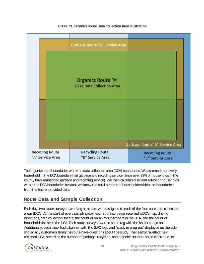
59 King County Waste Monitoring 2018 Task 1: Residential Curbside Characterization
Figure 73. Organics Route Data Collection Area Illustration
The organic route boundaries were the data collection area (DCA) boundaries. We assumed that every household in the DCA boundary had garbage and recycling service (since over 99% of households in the county have embedded garbage and recycling service). We then calculated set-out rates for households within the DCA boundaries because we knew the total number of households within the boundaries from the hauler provided data.
Route Data and Sample Collection
Each day, two route surveyors working as a team were assigned to each of the four base data collection areas (DCA). At the start of every sampling day, each route surveyor received a DCA map, driving directions, data collection sheets, the count of organics subscribers in the DCA, and the count of households in the in the DCA. Each route surveyor wore a name tag with the hauler’s logo on it. Additionally, each truck had a banner with the SWD logo and “study in progress” displayed on the side, should any customers along the route have questions about the study. The teams travelled their assigned DCA, recording the number of garbage, recycling, and organics set-outs on an electronic set-
60 King County Waste Monitoring 2018 Task 1: Residential Curbside Characterization
out count form. Paper field forms were available as a back-up to the electronic entry forms. An example of the set-out count form is included in Appendix E: Example Field Forms.
The route surveyors traversed the DCA 30 minutes before the hauler begins collection. This ensured that the sampler was sufficiently ahead of the hauler to prevent any disruptions to collection operations while allowing residents the maximum time to set out their carts for counting and collection.
Cascadia informed both the haulers and local police in the areas we were collecting samples of our sampling and collection plan the week prior to the start of sampling to ensure that all channels were properly informed should resident questions or interactions come up. We also had handouts with information about the study to provide to customers with questions about the study. Cascadia also tracked the number and type of customer interactions that occurred during the study, including recording the addresses of any customers who opt out of the study so they could be excluded from future rounds of sample collection. Examples of a customer handout and interaction tracking form are included in Appendix E: Example Field Forms.
The route survey teams were also responsible for selecting set-outs for sampling. Using a predetermined sampling interval, each route survey team collected all material from eight set-outs each day. The sampling interval was determined using the following procedure:
1. For each sampling day and DCA, the expected number of set-outs, L, was estimated using organics route data provided by the haulers. The number L was then reduced by one-fifth (producing 0.8 x L). This was done to ensure that the targeted number of set-outs were selected on each sampling day, even if there were fewer set-outs than expected.
2. Next, the interval n was determined to ensure systematic sampling of set-outs. If r represented the number of samples needed, and .8 x L represented the number of expected set-outs, then
( ) rLn ¸´= 8. ; every nth set-out were selected for sampling. To help facilitate this process, the sampling interval was noted on the set-out count form.
All the material from a single stream from each set-out constituted a sample. Each sample was stored and labeled separately. An example sample label is included in Appendix E: Example Field Forms. After the route survey team completed their DCA they transported the samples to the sorting facility.
Sorting Procedures
The goal was for all material set out from approximately 32 households were sorted each day for each sampling event, approximately 160 households total for each field event. The sorting procedure included the following four steps.
Step 1: Review methodology and sorting categories with the crew. To provide consistent sorting, Cascadia used highly trained crewmembers throughout the project. Before the sorting began, all crewmembers reviewed the procedures, forms, and material definitions. The material definitions are included in Appendix A: Material Type Definitions.
Step 2: Sort Sample. Once the sample was placed on the sorting table, two- to three-person sorting crews sorted material by hand into the prescribed material categories. The sorting crew manager monitored the accuracy of sorting, rejecting materials improperly classified.
61 King County Waste Monitoring 2018 Task 1: Residential Curbside Characterization
Step 3: Weigh the Sample. The field crew manager verified the purity of each material as it was weighed using a pre-tared scale and recorded the data on the sample tally sheet. An example of a sample tally sheet is included in Appendix E: Example Field Forms.
Step 4: Review Data. At the conclusion of each sorting day, the field crew manager conducted a quality control review of the data recorded.
The sample selection, collection, and sorting process is summarized in Figure 74.
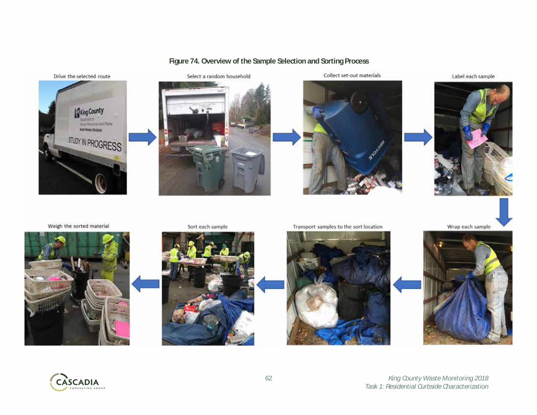
62 King County Waste Monitoring 2018 Task 1: Residential Curbside Characterization
Figure 74. Overview of the Sample Selection and Sorting Process
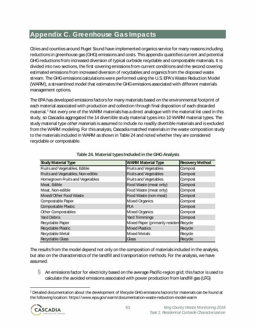
63 King County Waste Monitoring 2018 Task 1: Residential Curbside Characterization
Appendix C. Greenhouse Gas Impacts
Cities and counties around Puget Sound have implemented organics service for many reasons including reductions in greenhouse gas (GHG) emissions and costs. This appendix quantifies current and potential GHG reductions from increased diversion of typical curbside recyclable and compostable materials. It is divided into two sections, the first covering emissions from current conditions and the second covering estimated emissions from increased diversion of recyclables and organics from the disposed waste stream. The GHG emissions calculations were performed using the U.S. EPA’s Waste Reduction Model (WARM), a streamlined model that estimates the GHG emissions associated with different materials management options.
The EPA has developed emissions factors for many materials based on the environmental footprint of each material associated with production and collection through final disposition of each discarded material.1 Not every one of the WARM materials has a direct analogue with the material list used in this study, so Cascadia aggregated the 14 divertible study material types into 10 WARM material types. The study material type other materials is assumed to include no readily divertible materials and is excluded from the WARM modeling. For this analysis, Cascadia matched materials in the waste composition study to the materials included in WARM as shown in Table 24 and noted whether they are considered recyclable or compostable.
Table 24. Material types Included in the GHG Analysis
The results from the model depend not only on the composition of materials included in the analysis, but also on the characteristics of the landfill and transportation methods. For the analysis, we have assumed:
§ An emissions factor for electricity based on the average Pacific-region grid; this factor is used to calculate the avoided emissions associated with power production from landfill gas (LFG)
1 Detailed documentation about the development of lifecycle GHG emissions factors for materials can be found at the following location: https://www.epa.gov/warm/documentation-waste-reduction-model-warm
Study Material Type WARM Material Type Recovery MethodFruits and Vegetables, Edible Fruits and Vegetables CompostFruits and Vegetables, Non-edible Fruits and Vegetables CompostHomegrown Fruits and Vegetables Fruits and Vegetables CompostMeat, Edible Food Waste (meat only) CompostMeat, Non-edible Food Waste (meat only) CompostMixed/Other Food Waste Food Waste (non-meat) CompostCompostable Paper Mixed Organics CompostCompostable Plastic PLA CompostOther Compostables Mixed Organics CompostYard Debris Yard Trimmings CompostRecyclable Paper Mixed Paper (primarily residentRecycleRecyclable Plastic Mixed Plastics RecycleRecyclable Metal Mixed Metals RecycleRecyclable Glass Glass Recycle
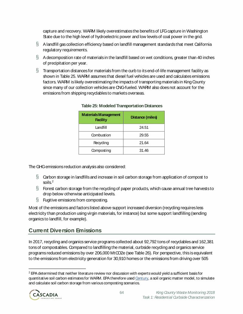
64 King County Waste Monitoring 2018 Task 1: Residential Curbside Characterization
capture and recovery. WARM likely overestimates the benefits of LFG capture in Washington State due to the high level of hydroelectric power and low levels of coal power in the grid.
§ A landfill gas collection efficiency based on landfill management standards that meet California regulatory requirements.
§ A decomposition rate of materials in the landfill based on wet conditions, greater than 40 inches of precipitation per year.
§ Transportation distances for materials from the curb to its end-of-life management facility as shown in Table 25. WARM assumes that diesel fuel vehicles are used and calculates emissions factors. WARM is likely overestimating the impacts of transporting materials in King County since many of our collection vehicles are CNG-fueled. WARM also does not account for the emissions from shipping recyclables to markets overseas.
Table 25: Modeled Transportation Distances
Materials Management Facility
Distance (miles)
Landfill 24.51
Combustion 29.55
Recycling 21.64
Composting 31.46
The GHG emissions reduction analysis also considered:
§ Carbon storage in landfills and increase in soil carbon storage from application of compost to soils.2
§ Forest carbon storage from the recycling of paper products, which cause annual tree harvests to drop below otherwise anticipated levels.
§ Fugitive emissions from composting.
Most of the emissions and factors listed above support increased diversion (recycling requires less electricity than production using virgin materials, for instance) but some support landfilling (sending organics to landfill, for example).
Current Diversion Emissions
In 2017, recycling and organics service programs collected about 92,792 tons of recyclables and 162,381 tons of compostables. Compared to landfilling the material, curbside recycling and organics service programs reduced emissions by over 206,000 MtCO2e (see Table 26). For perspective, this is equivalent to the emissions from electricity generation for 30,910 homes or the emissions from driving over 505
2 EPA determined that neither literature review nor discussion with experts would yield a sufficient basis for quantitative soil carbon estimates for WARM. EPA therefore used Century, a soil organic matter model, to simulate and calculate soil carbon storage from various composting scenarios.
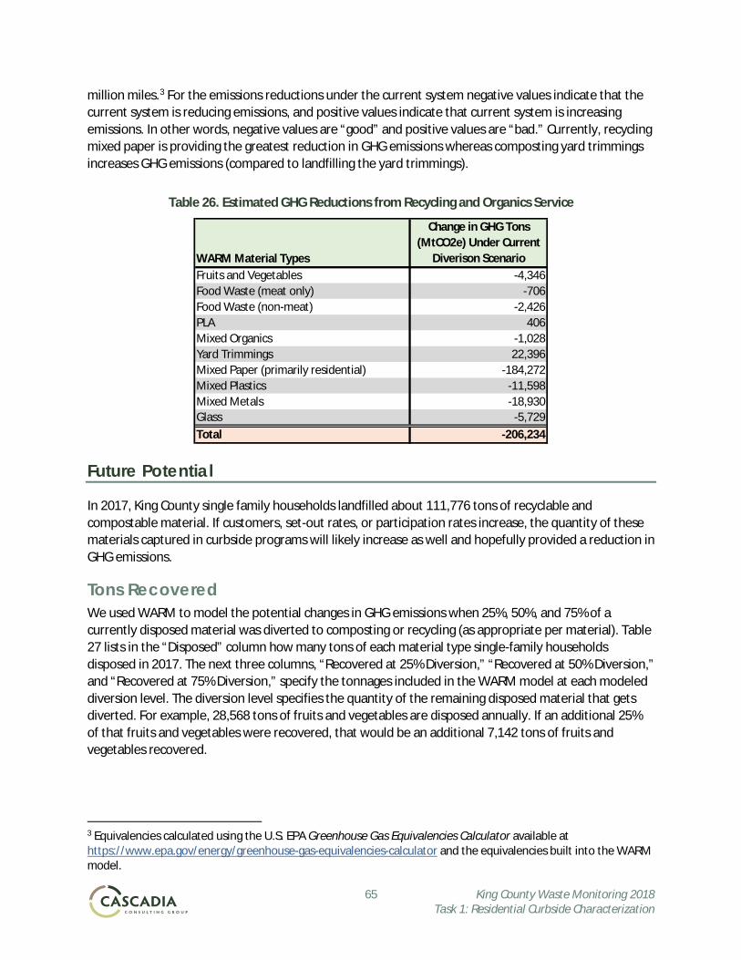
65 King County Waste Monitoring 2018 Task 1: Residential Curbside Characterization
million miles.3 For the emissions reductions under the current system negative values indicate that the current system is reducing emissions, and positive values indicate that current system is increasing emissions. In other words, negative values are “good” and positive values are “bad.” Currently, recycling mixed paper is providing the greatest reduction in GHG emissions whereas composting yard trimmings increases GHG emissions (compared to landfilling the yard trimmings).
Table 26. Estimated GHG Reductions from Recycling and Organics Service
Future Potential
In 2017, King County single family households landfilled about 111,776 tons of recyclable and compostable material. If customers, set-out rates, or participation rates increase, the quantity of these materials captured in curbside programs will likely increase as well and hopefully provided a reduction in GHG emissions.
Tons Recovered We used WARM to model the potential changes in GHG emissions when 25%, 50%, and 75% of a currently disposed material was diverted to composting or recycling (as appropriate per material). Table 27 lists in the “Disposed” column how many tons of each material type single-family households disposed in 2017. The next three columns, “Recovered at 25% Diversion,” “Recovered at 50% Diversion,” and “Recovered at 75% Diversion,” specify the tonnages included in the WARM model at each modeled diversion level. The diversion level specifies the quantity of the remaining disposed material that gets diverted. For example, 28,568 tons of fruits and vegetables are disposed annually. If an additional 25% of that fruits and vegetables were recovered, that would be an additional 7,142 tons of fruits and vegetables recovered.
3 Equivalencies calculated using the U.S. EPA Greenhouse Gas Equivalencies Calculator available at https://www.epa.gov/energy/greenhouse-gas-equivalencies-calculator and the equivalencies built into the WARM model.
WARM Material TypesFruits and Vegetables -4,346Food Waste (meat only) -706Food Waste (non-meat) -2,426PLA 406Mixed Organics -1,028Yard Trimmings 22,396Mixed Paper (primarily residential) -184,272Mixed Plastics -11,598Mixed Metals -18,930Glass -5,729Total -206,234
Change in GHG Tons (MtCO2e) Under Current
Diverison Scenario
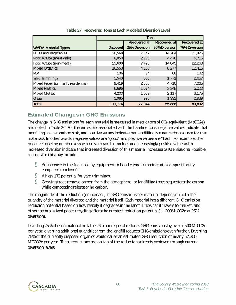
66 King County Waste Monitoring 2018 Task 1: Residential Curbside Characterization
Table 27. Recovered Tons at Each Modeled Diversion Level
Estimated Changes in GHG Emissions The change in GHG emissions for each material is measured in metric tons of CO2 equivalent (MtCO2e) and noted in Table 26. For the emissions associated with the baseline tons, negative values indicate that landfilling is a net carbon sink, and positive values indicate that landfilling is a net carbon source for that materials. In other words, negative values are “good” and positive values are “bad.” For example, the negative baseline numbers associated with yard trimmings and increasingly positive values with increased diversion indicate that increased diversion of this material increases GHG emissions. Possible reasons for this may include:
§ An increase in the fuel used by equipment to handle yard trimmings at a compost facility compared to a landfill.
§ A high LFG potential for yard trimmings. § Growing trees remove carbon from the atmosphere, so landfilling trees sequesters the carbon
while composting releases the carbon.
The magnitude of the reduction (or increase) in GHG emissions per material depends on both the quantity of the material diverted and the material itself. Each material has a different GHG emission reduction potential based on how readily it degrades in the landfill, how far it travels to market, and other factors. Mixed paper recycling offers the greatest reduction potential (11,203MtCO2e at 25% diversion).
Diverting 25% of each material in Table 26 from disposal reduces GHG emissions by over 7,500 MtCO2e per year; diverting additional quantities from the landfill reduces GHG emissions even further. Diverting 75% of the currently disposed organics would cause an estimated GHG reduction of nearly 52,300 MTCO2e per year. These reductions are on top of the reductions already achieved through current diversion levels.
WARM Material Types DisposedRecovered at
25% DiversionRecovered at
50% DiversionRecovered at
75% DiversionFruits and Vegetables 28,568 7,142 14,284 21,426Food Waste (meat only) 8,953 2,238 4,476 6,715Food Waste (non-meat) 29,690 7,423 14,845 22,268Mixed Organics 16,553 4,138 8,277 12,415PLA 136 34 68 102Yard Trimmings 3,543 886 1,771 2,657Mixed Paper (primarily residential) 9,419 2,355 4,710 7,065Mixed Plastics 6,696 1,674 3,348 5,022Mixed Metals 4,233 1,058 2,117 3,175Glass 3,985 996 1,992 2,989Total 111,776 27,944 55,888 83,832
Tons
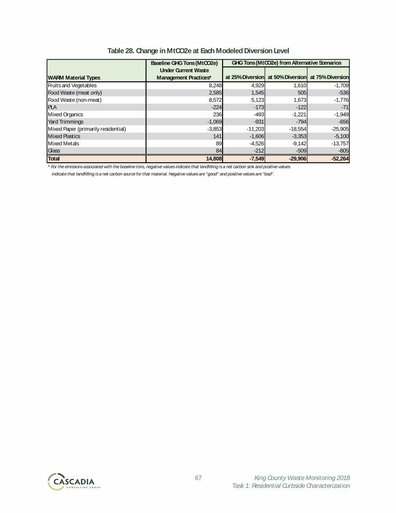
67 King County Waste Monitoring 2018 Task 1: Residential Curbside Characterization
Table 28. Change in MtCO2e at Each Modeled Diversion Level
WARM Material Types at 25% Diversion at 50% Diversion at 75% DiversionFruits and Vegetables 8,248 4,929 1,610 -1,709Food Waste (meat only) 2,585 1,545 505 -536Food Waste (non-meat) 8,572 5,123 1,673 -1,776PLA -224 -173 -122 -71Mixed Organics 236 -493 -1,221 -1,949Yard Trimmings -1,069 -931 -794 -656Mixed Paper (primarily residential) -3,853 -11,203 -18,554 -25,905Mixed Plastics 141 -1,606 -3,353 -5,100Mixed Metals 89 -4,526 -9,142 -13,757Glass 84 -212 -509 -805Total 14,808 -7,549 -29,906 -52,264* For the emissions associated with the baseline tons, negative values indicate that landfilling is a net carbon sink and positive values
indicate that landfilling is a net carbon source for that material. Negative values are "good" and positive values are "bad".
GHG Tons (MtCO2e) from Alternative ScenariosBaseline GHG Tons (MtCO2e) Under Current Waste
Management Practices*

68 King County Waste Monitoring 2018 Task 1: Residential Curbside Characterization
Appendix D: Calculations
Estimating Composition
Composition estimates were calculated using a method that gave equal weighting or “importance” to each sample. Confidence intervals (error ranges) were calculated based on assumptions of normality in the composition estimates.
In the descriptions of calculation methods, the following variables are used frequently:
§ i denotes an individual sample § j denotes the material type § cj is the weight of the material type j in a sample § w is the weight of an entire sample § rj is the composition estimate for material j (r stands for ratio) § s denotes a particular sector or subsector of the organics stream § n denotes the number of samples in the particular group that is being analyzed at that step
Estimating the Composition For a given sampling stratum, the composition estimate denoted by rj represents the ratio of the component’s weight to the total weight of all the samples in the stratum. This estimate was derived by summing each component’s weight across all the selected samples belonging to a given stratum and dividing by the sum of the total weight for all the samples in that stratum, as shown in the following equation:
where:
§ c = weight of particular component § w = sum of all component weights § for i = 1 to n, where n = number of selected samples § for j = 1 to m, where m = number of components
rc
wj
iji
ii
=åå
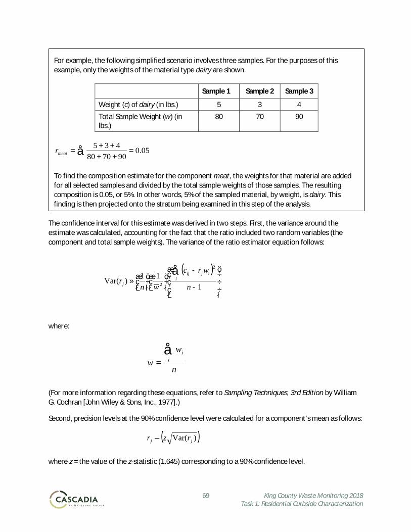
69 King County Waste Monitoring 2018 Task 1: Residential Curbside Characterization
The confidence interval for this estimate was derived in two steps. First, the variance around the estimate was calculated, accounting for the fact that the ratio included two random variables (the component and total sample weights). The variance of the ratio estimator equation follows:
where:
(For more information regarding these equations, refer to Sampling Techniques, 3rd Edition by William G. Cochran [John Wiley & Sons, Inc., 1977].)
Second, precision levels at the 90% confidence level were calculated for a component’s mean as follows:
where z = the value of the z-statistic (1.645) corresponding to a 90% confidence level.
For example, the following simplified scenario involves three samples. For the purposes of this example, only the weights of the material type dairy are shown.
Sample 1 Sample 2 Sample 3
Weight (c) of dairy (in lbs.) 5 3 4
Total Sample Weight (w) (in lbs.)
80 70 90
To find the composition estimate for the component meat, the weights for that material are added for all selected samples and divided by the total sample weights of those samples. The resulting composition is 0.05, or 5%. In other words, 5% of the sampled material, by weight, is dairy. This finding is then projected onto the stratum being examined in this step of the analysis.
05.0907080
435=
++++
= åmeatr
( )
÷÷÷
ø
ö
ççç
è
æ
-
-÷øö
çèæ
÷øö
çèæ»
å1
11)Var(
2
2 n
wrc
wnr i
ijij
j
ww
n
ii=
å
( ))Var( jj rzr ±
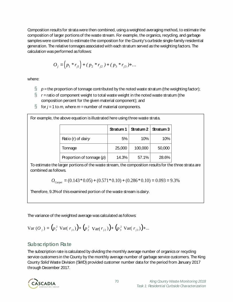
70 King County Waste Monitoring 2018 Task 1: Residential Curbside Characterization
Composition results for strata were then combined, using a weighted averaging method, to estimate the composition of larger portions of the waste stream. For example, the organics, recycling, and garbage samples were combined to estimate the composition for the County’s curbside single-family residential generation. The relative tonnages associated with each stratum served as the weighting factors. The calculation was performed as follows:
where:
§ p = the proportion of tonnage contributed by the noted waste stratum (the weighting factor); § r = ratio of component weight to total waste weight in the noted waste stratum (the
composition percent for the given material component); and § for j = 1 to m, where m = number of material components.
The variance of the weighted average was calculated as follows:
Subscription Rate The subscription rate is calculated by dividing the monthly average number of organics or recycling service customers in the County by the monthly average number of garbage service customers. The King County Solid Waste Division (SWD) provided customer number data for the period from January 2017 through December 2017.
( )O p r p r p rj j j j= + + +1 1 2 2 3 3* ( * ) ( * ) ...
For example, the above equation is illustrated here using three waste strata.
Stratum 1 Stratum 2 Stratum 3
Ratio (r) of dairy 5% 10% 10%
Tonnage 25,000 100,000 50,000
Proportion of tonnage (p) 14.3% 57.1% 28.6%
To estimate the larger portions of the waste stream, the composition results for the three strata are combined as follows.
%3.9093.0)10.0*286.0()10.0*571.0()05.0*143.0( ==++=CarpetO
Therefore, 9.3% of this examined portion of the waste stream is dairy.
( ) ( ) ( ) +... + + = ) Var( ) Var( ) Var( ) ( Var 3 2 3 2
2 2 1
2 1 j j j j r p r p r p O
71 King County Waste Monitoring 2018 Task 1: Residential Curbside Characterization
𝑎𝑎𝑎𝑎𝑎𝑎.𝑚𝑚𝑚𝑚𝑚𝑚𝑚𝑚ℎ𝑙𝑙𝑙𝑙 𝑚𝑚𝑜𝑜𝑜𝑜𝑎𝑎𝑚𝑚𝑜𝑜𝑜𝑜𝑜𝑜 𝑚𝑚𝑜𝑜 𝑜𝑜𝑎𝑎𝑜𝑜𝑙𝑙𝑜𝑜𝑙𝑙𝑜𝑜𝑚𝑚𝑜𝑜 𝑜𝑜𝑐𝑐𝑜𝑜𝑚𝑚𝑚𝑚𝑚𝑚𝑎𝑎𝑜𝑜𝑜𝑜 ÷ 𝑎𝑎𝑎𝑎𝑎𝑎.𝑚𝑚𝑚𝑚𝑚𝑚𝑚𝑚ℎ𝑙𝑙𝑙𝑙 𝑜𝑜𝑎𝑎𝑜𝑜𝑔𝑔𝑎𝑎𝑜𝑜𝑎𝑎 𝑜𝑜𝑐𝑐𝑜𝑜𝑚𝑚𝑚𝑚𝑚𝑚𝑎𝑎𝑜𝑜𝑜𝑜 = 𝑜𝑜𝑐𝑐𝑔𝑔𝑜𝑜𝑜𝑜𝑜𝑜𝑜𝑜𝑠𝑠𝑚𝑚𝑜𝑜𝑚𝑚𝑚𝑚 𝑜𝑜𝑎𝑎𝑚𝑚𝑎𝑎
Set-out Rate The set-out rate is calculated by dividing the total number of carts set out from each stream for along surveyed routes by the total number of customers for each stream along surveyed routes. For the purposes of this study all households were assumed to be garbage customers and recycling customers. In jurisdictions with embedded organics service all households were assumed to be organics customers. In jurisdictions with subscription organics service the haulers provided the number of organics customers on the surveyed organics routes.
𝑚𝑚𝑐𝑐𝑚𝑚𝑔𝑔𝑎𝑎𝑜𝑜 𝑚𝑚𝑜𝑜 𝑜𝑜𝑎𝑎𝑚𝑚 𝑚𝑚𝑐𝑐𝑚𝑚𝑜𝑜 𝑚𝑚𝑚𝑚 𝑜𝑜𝑚𝑚𝑐𝑐𝑚𝑚𝑎𝑎𝑜𝑜 ÷ 𝑚𝑚𝑐𝑐𝑚𝑚𝑔𝑔𝑎𝑎𝑜𝑜 𝑚𝑚𝑜𝑜 𝑜𝑜𝑐𝑐𝑜𝑜𝑚𝑚𝑚𝑚𝑚𝑚𝑎𝑎𝑜𝑜𝑜𝑜 𝑚𝑚𝑚𝑚 𝑜𝑜𝑚𝑚𝑐𝑐𝑚𝑚𝑎𝑎𝑜𝑜 = 𝑜𝑜𝑎𝑎𝑚𝑚 𝑚𝑚𝑐𝑐𝑚𝑚 𝑜𝑜𝑎𝑎𝑚𝑚𝑎𝑎
Participation Rate The customer participation rate for any material is a measure of the people who have signed up for a service (not all households organics service even if it’s available) that place the material of interest in the correct cart (recyclables in the recycling cart and organics in the organics cart). Placing recyclables in an organics cart does not count when calculating the participation rate. The set-out participation rate is a measure of the number of carts set out for collection that contain the material of interest.
For example, the set-out food scraps participation rate is calculated by dividing the number of samples that contained food scraps by the total number of samples collected.
(𝑜𝑜𝑎𝑎𝑚𝑚𝑠𝑠𝑙𝑙𝑎𝑎𝑜𝑜 𝑤𝑤𝑜𝑜𝑚𝑚ℎ 𝑜𝑜𝑚𝑚𝑚𝑚𝑓𝑓 𝑜𝑜𝑜𝑜𝑜𝑜𝑎𝑎𝑠𝑠𝑜𝑜) ÷ (𝑚𝑚𝑚𝑚𝑚𝑚𝑎𝑎𝑙𝑙 𝑜𝑜𝑎𝑎𝑚𝑚𝑠𝑠𝑙𝑙𝑎𝑎𝑜𝑜)= 𝑜𝑜𝑎𝑎𝑚𝑚 𝑚𝑚𝑐𝑐𝑚𝑚 𝑜𝑜𝑚𝑚𝑚𝑚𝑓𝑓 𝑜𝑜𝑜𝑜𝑜𝑜𝑎𝑎𝑠𝑠𝑜𝑜 𝑠𝑠𝑎𝑎𝑜𝑜𝑚𝑚𝑜𝑜𝑜𝑜𝑜𝑜𝑠𝑠𝑎𝑎𝑚𝑚𝑜𝑜𝑚𝑚𝑚𝑚 𝑜𝑜𝑎𝑎𝑚𝑚𝑎𝑎
The customer food scraps participation rate is calculated by multiplying the set-out food scraps participation rate by the set-out rate. The premise is that we know what percent of set-outs have food scraps and we know what percent of customers set their carts out, so the percent of customers who participate is the product of those two numbers.
(𝑜𝑜𝑎𝑎𝑚𝑚 𝑚𝑚𝑐𝑐𝑚𝑚 𝑜𝑜𝑎𝑎𝑚𝑚𝑎𝑎) × (𝑜𝑜𝑎𝑎𝑚𝑚 𝑚𝑚𝑐𝑐𝑚𝑚 𝑜𝑜𝑚𝑚𝑚𝑚𝑓𝑓 𝑜𝑜𝑜𝑜𝑜𝑜𝑎𝑎𝑠𝑠𝑜𝑜 𝑠𝑠𝑎𝑎𝑜𝑜𝑚𝑚𝑜𝑜𝑜𝑜𝑜𝑜𝑠𝑠𝑎𝑎𝑚𝑚𝑚𝑚𝑚𝑚 𝑜𝑜𝑎𝑎𝑚𝑚𝑎𝑎)= 𝑜𝑜𝑐𝑐𝑜𝑜𝑚𝑚𝑚𝑚𝑚𝑚𝑎𝑎𝑜𝑜 𝑜𝑜𝑚𝑚𝑚𝑚𝑓𝑓 𝑜𝑜𝑜𝑜𝑜𝑜𝑎𝑎𝑠𝑠𝑜𝑜 𝑠𝑠𝑎𝑎𝑜𝑜𝑚𝑚𝑜𝑜𝑜𝑜𝑜𝑜𝑠𝑠𝑎𝑎𝑚𝑚𝑜𝑜𝑚𝑚𝑚𝑚 𝑜𝑜𝑎𝑎𝑚𝑚𝑎𝑎
Evaluating Changes in the Composition Between Studies
Comparisons examined the changes in the composition percentages for each of four material groups. To control for population changes and other factors that may influence the total amount of material composted from year to year, the tests described in this appendix measure material proportions, not actual tonnage. For example, say that Food accounts for 10% of composted material each year, and that a total of 1,000 tons of material was composted in one year and 2,000 tons composted in the next. While the amount of Food increased from 1,000 to 2,000 tons, the percentage remained the same. Therefore, the tests would indicate that there had been no change.
The purpose of conducting these comparisons is to identify trends within the organics stream in the percentage of selected types of waste disposed over time. One specific example is stated as follows:
72 King County Waste Monitoring 2018 Task 1: Residential Curbside Characterization
Hypothesis: “There is no statistically significant difference, between the 2014 and 2017 study periods, in the percentage of Food composted.”
Statistics are then employed to look for evidence disproving the hypothesis. A “significant” result means that there is enough evidence to disprove the hypothesis and it can be concluded that there is a true difference across years. “Insignificant” results indicate that either a) there is no true difference, or b) even though there may be a difference, there is not enough evidence to prove it.4
The purpose of these tests is to identify changes across years; however, the study did not attempt to investigate why or how these changes occurred. The changes may be due to a variety of. Future studies could be designed to test the influence of various potential sources of the increase/decrease of specific materials in the disposed waste stream.
Statistical Considerations The analyses were based on the component percentages, by weight. As described in Appendix D: Calculations, these percentages are calculated by dividing the sum of the selected component weights by the sum of the corresponding sample weights. T-tests (modified for ratio estimation) were used to examine the variations from year to year.
Normality The distributions of some of the material types may be skewed and may not follow a normal distribution. Although t-tests assume a normal distribution, they are very robust to departures from this assumption, particularly with large sample sizes. In addition, the material classes are sums of the material types, which improve our ability to meet the assumptions of normality.
Dependence There may be dependence between material types (i.e., if a person disposes of material A, they always dispose of material B at the same time).
There is certainly a degree of dependence between the calculated percentages. Because the percentages sum to 100 (in the case of year-to-year comparisons), if the percentage of material A increases, the percentage of some other material must decrease.
Multiple T-Tests In all statistical tests, there is a chance of incorrectly concluding that a result is significant. The year-to-year comparison required conducting several t-tests (one for each material class), each of which carries that risk. However, we were willing to accept only a 10% chance, overall, of making an incorrect
conclusion. Therefore, each test was adjusted by setting the significance threshold to 010.w
(w = the
number of t-tests).
The adjustment can be explained as follows:
4 Please see the “Power Analysis” discussion on page 69.

73 King County Waste Monitoring 2018 Task 1: Residential Curbside Characterization
For each test, we set a 1 010-
.w
chance of not making a mistake, which results in a 1 010-æ
èçöø÷
.w
wchance
of not making a mistake during all w tests.
Since one minus the chance of not making a mistake equals the chance of making a mistake, by making this adjustment, we have set the overall risk of making a wrong conclusion during any one of the tests at
1 1 010 010- -æèç
öø÷
æ
èçç
ö
ø÷÷ =
. .w
w
.
The chance of a “false positive” for the year-to-year comparisons made in this study is restricted to 10% overall, or 2.5% for each test (10% divided by the four tests equals 2.5%).
For more detail regarding this issue, please refer to Section 11.2 “The Multiplicity Problem and the Bonferroni Inequality” of An Introduction to Contemporary Statistics by L.H. Koopmans (Duxbury Press, 1981).
Power Analysis As the number of samples is increased, so is the ability to detect differences. In the future, an a priori power analysis might benefit this research by determining how many samples would be required to detect a particular minimum difference of interest.
Interpreting the Calculation Results For the purposes of this study, only those calculation results with a p-value of less than 2.5% are considered to be statistically significant. As described above, the threshold for determining statistically significant results (the “alpha-level”) is conservative, accounting for the fact that so many individual tests were calculated.
The t-statistic is calculated from the data. According to statistical theory, the larger the absolute value of the t-statistic, the less likely the two populations are to have the same mean. The p-value describes the probability of observing the calculated t-statistic if there were no true difference between the population means.
74 King County Waste Monitoring 2018 Task 1: Residential Curbside Characterization
Appendix E: Example Field Forms
This appendix contains examples of the field forms used throughout the study, including:
§ Set Out Count Form § Sample Label § Sample Tally Sheet § Customer Hand Out § Customer Interaction Tracking Form
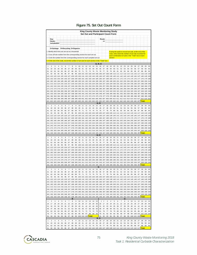
75 King County Waste Monitoring 2018 Task 1: Residential Curbside Characterization
Figure 75. Set Out Count Form
King County Waste Monitoring StudySet Out and Participant Count Form
Day: Route:Hauler: n=Jurisdiction:
G=Garbage R=Recycling O=Organics
1. Identify which bins are set out at a household
2. Cross off one number from the corresponding section for each set out
3. Circle the number from the corresponding section for each sampled set out
4. At the end of the route, record the number of set outs for each section in the "Total" box
G, R, O1 2 3 4 5 6 7 8 9 10 11 12 13 14 15 16 17 18 19 20 21 22 23 24 25 26 27 28 29 30
31 32 33 34 35 36 37 38 39 40 41 42 43 44 45 46 47 48 49 50 51 52 53 54 55 56 57 58 59 6061 62 63 64 65 66 67 68 69 70 71 72 73 74 75 76 77 78 79 80 81 82 83 84 85 86 87 88 89 9091 92 93 94 95 96 97 98 99 100 101 102 103 104 105 106 107 108 109 110 111 112 113 114 115 116 117 118 119 120121 122 123 124 125 126 127 128 129 130 131 132 133 134 135 136 137 138 139 140 141 142 143 144 145 146 147 148 149 150151 152 153 154 155 156 157 158 159 160 161 162 163 164 165 166 167 168 169 170 171 172 173 174 175 176 177 178 179 180181 182 183 184 185 186 187 188 189 190 191 192 193 194 195 196 197 198 199 200 201 202 203 204 205 206 207 208 209 210211 212 213 214 215 216 217 218 219 220 221 222 223 224 225 226 227 228 229 230 231 232 233 234 235 236 237 238 239 240241 242 243 244 245 246 247 248 249 250 251 252 253 254 255 256 257 258 259 260 261 262 263 264 265 266 267 268 269 270271 272 273 274 275 276 277 278 279 280 281 282 283 284 285 286 287 288 289 290 291 292 293 294 295 296 297 298 299 300301 302 303 304 305 306 307 308 309 310 311 312 313 314 315 316 317 318 319 320 321 322 323 324 325 326 327 328 329 330331 332 333 334 335 336 337 338 339 340 341 342 343 344 345 346 347 348 349 350 351 352 353 354 355 356 357 358 359 360361 362 363 364 365 366 367 368 369 370 371 372 373 374 375 376 377 378 379 380 381 382 383 384 385 386 387 388 389 390391 392 393 394 395 396 397 398 399 400 401 402 403 404 405 406 407 408 409 410 411 412 413 414 415 416 417 418 419 420421 422 423 424 425 426 427 428 429 430 431 432 433 434 435 436 437 438 439 440 441 442 443 444 445 446 447
G, R1 2 3 4 5 6 7 8 9 10 11 12 13 14 15 16 17 18 19 20 21 22 23 24 25 26 27 28 29 30
31 32 33 34 35 36 37 38 39 40 41 42 43 44 45 46 47 48 49 50 51 52 53 54 55 56 57 58 59 6061 62 63 64 65 66 67 68 69 70 71 72 73 74 75 76 77 78 79 80 81 82 83 84 85 86 87 88 89 9091 92 93 94 95 96 97 98 99 100 101 102 103 104 105 106 107 108 109 110 111 112 113 114 115 116 117 118 119 120121 122 123 124 125 126 127 128 129 130 131 132 133 134 135 136 137 138 139 140 141 142 143 144 145 146 147 148 149 150151 152 153 154 155 156 157 158 159 160 161 162 163 164 165 166 167 168 169 170 171 172 173 174 175 176 177 178 179 180181 182 183 184 185 186 187 188 189 190 191 192 193 194 195 196 197 198 199 200 201 202 203 204 205 206 207 208 209 210211 212 213 214 215 216 217 218 219 220 221 222 223 224 225 226 227 228 229 230 231 232 233 234 235 236 237 238 239 240241 242 243 244 245 246 247 248 249 250 251 252 253 254 255 256 257 258 259 260 261 262 263 264 265 266 267 268 269 270271 272 273 274 275 276 277 278 279 280 281 282 283 284 285 286 287 288 289 290 291 292 293 294 295 296 297 298 299 300301 302 303 304 305 306 307 308 309 310 311 312 313 314 315 316 317 318 319 320 321 322 323 324 325 326 327 328 329 330331 332 333 334 335 336 337 338 339 340 341 342 343 344 345 346 347 348 349 350 351 352 353 354 355 356 357
G, O1 2 3 4 5 6 7 8 9 10 11 12 13 14 15 16 17 18 19 20 21 22 23 24 25 26 27 28 29 30
31 32 33 34 35 36 37 38 39 40 41 42 43 44 45 46 47 48 49 50 51 52 53 54 55 56 57 58 59 6061 62 63 64 65 66 67 68 69 70 71 72 73 74 75 76 77 78 79 80 81 82 83 84 85 86 87 88 89 9091 92 93 94 95 96 97 98 99 100 101 102 103 104 105 106 107 108 109 110 111 112 113 114 115 116 117 118 119 120121 122 123 124 125 126 127 128 129 130 131 132 133 134 135 136 137 138 139 140 141 142 143 144 145 146 147 148 149 150151 152 153 154 155 156 157 158 159 160 161 162 163 164 165 166 167 168 169 170 171 172 173 174 175 176 177 178 179 180181 182 183 184 185 186 187 188 189 190 191 192 193 194 195 196 197 198 199 200 201 202 203 204 205 206 207 208 209 210211 212 213 214 215 216 217 218 219 220 221 222 223 224 225 226 227 228 229 230 231 232 233 234 235 236 237 238 239 240241 242 243 244 245 246 247 248 249 250 251 252 253 254 255 256 257 258 259 260 261 262 263 264 265 266 267 268 269 270271 272 273 274 275 276 277 278 279 280 281 282 283 284 285 286 287 288 289 290 291 292 293 294 295 296 297 298 299 300301 302 303 304 305 306 307 308 309 310 311 312 313 314 315 316 317 318 319 320 321 322 323 324 325 326 327 328 329 330331 332 333 334 335 336 337 338 339 340 341 342 343 344 345 346 347 348 349 350 351 352 353 354 355 356 357
G1 2 3 4 5 6 7 8 9 10 11 12 13 14 15 16 17 18 19 20 21 22 23 24 25 26 27 28 29 30
31 32 33 34 35 36 37 38 39 40 41 42 43 44 45 46 47 48 49 50 51 52 53 54 55 56 57 58 59 6061 62 63 64 65 66 67 68 69 70 71 72 73 74 75 76 77 78 79 80 81 82 83 84 85 86 87 88 89 9091 92 93 94 95 96 97 98 99 100 101 102 103 104 105 106 107 108 109 110 111 112 113 114 115 116 117 118 119 120121 122 123 124 125 126 127 128 129 130 131 132 133 134 135 136 137 138 139 140 141 142 143 144 145 146 147 148 149 150151 152 153 154 155 156 157 158 159 160 161 162 163 164 165 166 167 168 169 170 171 172 173 174 175 176 177 178 179 180181 182 183 184 185 186 187 188 189 190 191 192 193 194 195 196 197 198 199 200 201 202 203 204 205 206 207 208 209 210211 212 213 214 215 216 217 218 219 220 221 222 223 224 225 226 227 228 229 230 231 232 233 234 235 236 237 238 239 240241 242 243 244 245 246 247 248 249 250 251 252 253 254 255 256 257 258 259 260 261 262 263 264 265 266 267 268 269 270271 272 273 274 275 276 277 278 279 280 281 282 283 284 285 286 287 288 289 290 291 292 293 294 295 296 297 298 299 300301 302 303 304 305 306 307 308 309 310 311 312 313 314 315 316 317 318 319 320 321 322 323 324 325 326 327 328 329 330331 332 333 334 335 336 337 338 339 340 341 342 343 344 345 346 347 348 349 350 351 352 353 354 355 356 357
R O1 2 3 4 5 6 7 8 9 10 11 12 13 14 15 1 2 3 4 5 6 7 8 9 10 11 12 13 14 15
16 17 18 19 20 21 22 23 24 25 26 27 28 29 30 16 17 18 19 20 21 22 23 24 25 26 27 28 29 3031 32 33 34 35 36 37 38 39 40 41 42 43 44 45 31 32 33 34 35 36 37 38 39 40 41 42 43 44 4546 47 48 49 50 51 52 53 54 55 56 57 58 59 60 46 47 48 49 50 51 52 53 54 55 56 57 58 59 6061 62 63 64 65 66 67 68 69 70 71 72 73 74 75 61 76 77 78 79 80 81 82 83 84 85 86 87 88 8976 77 78 79 80 81 82 83 84 85 86 87 88 89 90 76 91 92 93 94 95 96 97 98 99 100 101 102 103 10491 92 93 94 95 96 97 98 99 100 101 102 91 92 93 94 95 96 97 98 99 100 101 102
R, O1 2 3 4 5 6 7 8 9 10 11 12 13 14 15 16 17 18 19 20 21 22 23 24 25 26 27 28 29 3031 32 33 34 35 36 37 38 39 40 41 42 43 44 45 46 47 48 49 50 51 52 53 54 55 56 57 58 59 6061 62 63 64 65 66 67 68 69 70 71 72 73 74 75 76 77 78 79 80 81 82 83 84 85 86 87 88 89 9091 92 93 94 95 96 97 98 99 100 101 102 103 104 105 106 107 108 109 110 111 112 113 114 115 116 117 Total:
Total:
If using the ipads to record set outs, at the end of the route, write down the number of set outs recorded for each combination of carts in the "Total" box in each section
Total:
Total:
Total:
Total:
Total:
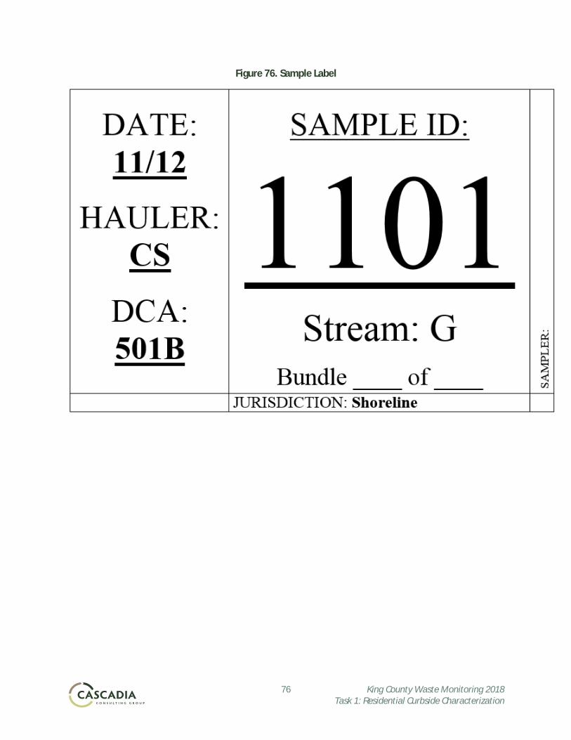
76 King County Waste Monitoring 2018 Task 1: Residential Curbside Characterization
Figure 76. Sample Label
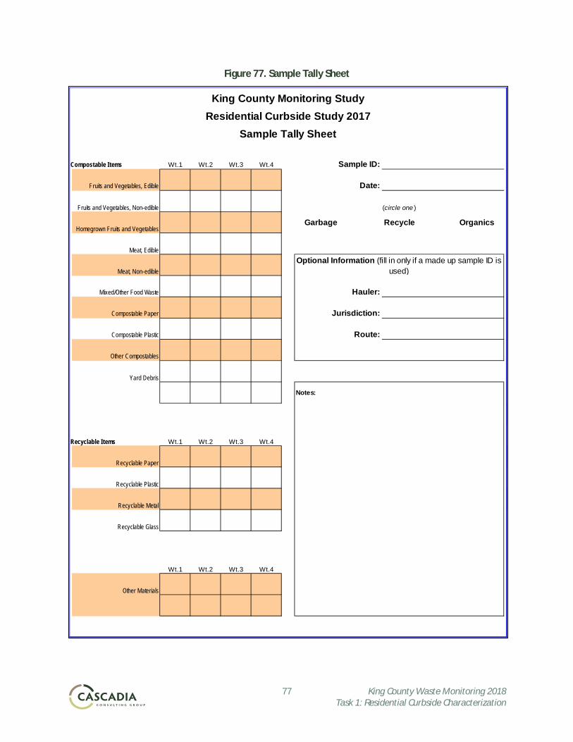
77 King County Waste Monitoring 2018 Task 1: Residential Curbside Characterization
Figure 77. Sample Tally Sheet
Compostable Items Wt.1 Wt.2 Wt.3 Wt.4 Sample ID:
Fruits and Vegetables, Edible Date:
Fruits and Vegetables, Non-edible
Homegrown Fruits and Vegetables
Meat, Edible
Meat, Non-edible
Mixed/Other Food Waste Hauler:
Compostable Paper Jurisdiction:
Compostable Plastic Route:
Other Compostables
Yard Debris
Notes:
Recyclable Items Wt.1 Wt.2 Wt.3 Wt.4
Recyclable Paper
Recyclable Plastic
Recyclable Metal
Recyclable Glass
Wt.1 Wt.2 Wt.3 Wt.4
Other Materials
Sample Tally SheetResidential Curbside Study 2017
King County Monitoring Study
Optional Information (fill in only if a made up sample ID is used)
Garbage Recycle Organics
(circle one )
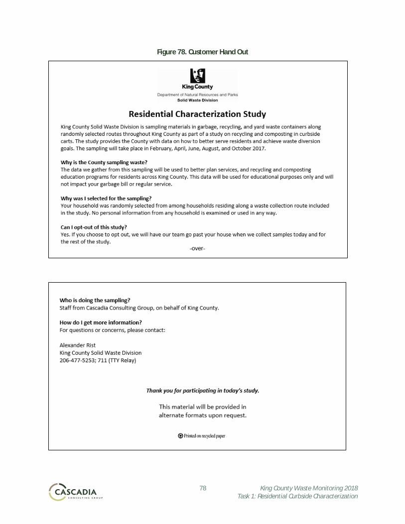
78 King County Waste Monitoring 2018 Task 1: Residential Curbside Characterization
Figure 78. Customer Hand Out
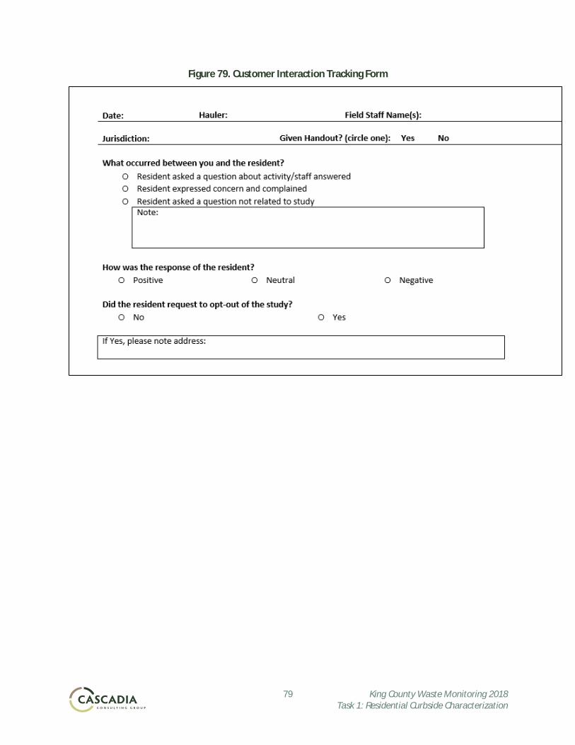
79 King County Waste Monitoring 2018 Task 1: Residential Curbside Characterization
Figure 79. Customer Interaction Tracking Form
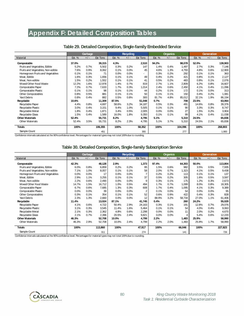
80 King County Waste Monitoring 2018 Task 1: Residential Curbside Characterization
Appendix F: Detailed Composition Tables
Table 29. Detailed Composition, Single-family Embedded Service
Table 30. Detailed Composition, Single-family Subscription Service
Garbage Recycling Organics Generation Material Est. % + / - Est Tons Est. % + / - Est Tons Est. % + / - Est Tons Est. % + / - Est Tons
Compostable 37.0% 39,315 4.3% 2,510 94.2% 98,078 52.0% 139,903 Fruits and Vegetables, Edible 5.2% 0.7% 5,502 0.3% 0.2% 147 1.4% 0.4% 1,497 2.7% 0.3% 7,146 Fruits and Vegetables, Non-edible 7.6% 0.9% 8,062 0.1% 0.0% 45 4.6% 1.3% 4,793 4.8% 0.6% 12,900 Homegrown Fruits and Vegetables 0.1% 0.1% 71 0.0% 0.0% - 0.3% 0.2% 292 0.1% 0.1% 363 Meat, Edible 1.6% 0.3% 1,656 0.1% 0.1% 49 0.4% 0.2% 421 0.8% 0.1% 2,127 Meat, Non-edible 1.5% 0.2% 1,552 0.1% 0.1% 41 0.5% 0.2% 483 0.8% 0.1% 2,076 Mixed/Other Food Waste 12.2% 1.6% 12,978 1.4% 0.7% 819 2.7% 1.1% 2,809 6.2% 0.8% 16,607 Compostable Paper 7.2% 0.7% 7,633 1.7% 0.3% 1,014 2.4% 0.6% 2,450 4.1% 0.4% 11,096 Compostable Plastic 0.1% 0.1% 98 0.1% 0.1% 44 0.2% 0.1% 172 0.1% 0.0% 313 Other Compostables 0.8% 0.5% 881 0.1% 0.1% 50 0.1% 0.1% 150 0.4% 0.2% 1,081 Yard Debris 0.8% 0.4% 882 0.5% 0.8% 300 81.7% 4.8% 85,012 32.1% 1.9% 86,194
Recyclable 10.6% 11,309 87.5% 51,048 0.7% 708 23.5% 63,064 Recyclable Paper 4.4% 0.8% 4,697 58.6% 3.2% 34,187 0.5% 0.3% 491 14.6% 0.8% 39,376 Recyclable Plastic 3.0% 0.4% 3,151 9.4% 1.0% 5,505 0.1% 0.1% 90 3.3% 0.3% 8,747 Recyclable Metal 1.8% 0.4% 1,871 3.4% 0.5% 2,005 0.0% 0.0% 27 1.5% 0.2% 3,904 Recyclable Glass 1.5% 0.4% 1,589 16.0% 1.8% 9,350 0.1% 0.1% 99 4.1% 0.4% 11,038
Other Materials 52.4% 55,731 8.2% 4,795 5.1% 5,310 24.5% 65,836 Other Materials 52.4% 3.5% 55,731 8.2% 2.3% 4,795 5.1% 3.7% 5,310 24.5% 2.1% 65,836
Totals 100% 106,355 100% 58,352 100% 104,096 100% 268,803Sample Count 451 355 277 1,083
Confidence intervals calculated at the 90% confidence level. Percentages for material types may not total 100% due to rounding.
Garbage Recycling Organics Generation Material Est. % + / - Est Tons Est. % + / - Est Tons Est. % + / - Est Tons Est. % + / - Est Tons
Compostable 42.3% 48,128 2.9% 1,373 97.4% 64,303 50.0% 113,804 Fruits and Vegetables, Edible 6.0% 0.8% 6,859 0.2% 0.2% 95 1.5% 0.6% 982 3.5% 0.5% 7,935 Fruits and Vegetables, Non-edible 7.1% 1.0% 8,057 0.1% 0.1% 58 2.0% 0.7% 1,323 4.1% 0.5% 9,438 Homegrown Fruits and Vegetables 0.0% 0.0% 17 0.0% 0.0% 7 0.2% 0.2% 113 0.1% 0.1% 137 Meat, Edible 2.9% 1.1% 3,255 0.1% 0.1% 37 0.5% 0.2% 305 1.6% 0.5% 3,597 Meat, Non-edible 2.2% 0.6% 2,490 0.0% 0.0% 9 0.3% 0.1% 175 1.2% 0.3% 2,673 Mixed/Other Food Waste 14.7% 1.5% 16,712 1.0% 0.5% 494 1.7% 0.7% 1,099 8.0% 0.8% 18,305 Compostable Paper 6.7% 0.6% 7,685 1.3% 0.3% 608 1.7% 0.4% 1,095 4.1% 0.3% 9,389 Compostable Plastic 0.0% 0.0% 39 0.0% 0.0% 2 0.1% 0.0% 54 0.0% 0.0% 95 Other Compostables 0.3% 0.1% 354 0.1% 0.1% 52 0.6% 0.9% 422 0.4% 0.3% 828 Yard Debris 2.3% 1.3% 2,660 0.0% 0.0% 12 88.9% 3.2% 58,734 27.0% 1.1% 61,406
Recyclable 11.4% 13,024 87.1% 41,745 0.4% 260 24.2% 55,029 Recyclable Paper 4.1% 0.6% 4,722 50.4% 2.9% 24,163 0.3% 0.1% 191 12.8% 0.7% 29,076 Recyclable Plastic 3.1% 0.3% 3,545 11.4% 1.6% 5,464 0.1% 0.1% 54 4.0% 0.4% 9,063 Recyclable Metal 2.1% 0.3% 2,362 4.8% 0.6% 2,298 0.0% 0.0% 11 2.0% 0.2% 4,670 Recyclable Glass 2.1% 0.7% 2,396 20.5% 2.4% 9,821 0.0% 0.0% 4 5.4% 0.6% 12,220
Other Materials 46.3% 52,708 10.0% 4,799 2.2% 1,483 25.9% 58,990 Other Materials 46.3% 2.9% 52,708 10.0% 2.4% 4,799 2.2% 2.0% 1,483 25.9% 1.7% 58,990
Totals 100% 113,860 100% 47,917 100% 66,046 100% 227,823Sample Count 311 274 141 726
Confidence intervals calculated at the 90% confidence level. Percentages for material types may not total 100% due to rounding.
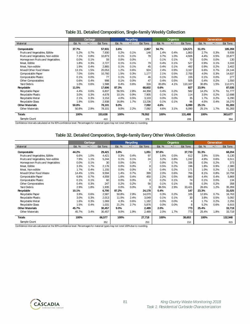
81 King County Waste Monitoring 2018 Task 1: Residential Curbside Characterization
Table 31. Detailed Composition, Single-family Weekly Collection
Table 32. Detailed Composition, Single-family Every Other Week Collection
Garbage Recycling Organics Generation Material Est. % + / - Est Tons Est. % + / - Est Tons Est. % + / - Est Tons Est. % + / - Est Tons
Compostable 37.7% 57,931 3.6% 2,857 94.7% 124,571 51.0% 185,359 Fruits and Vegetables, Edible 5.2% 0.7% 7,930 0.2% 0.1% 146 1.4% 0.4% 1,863 2.7% 0.3% 9,939 Fruits and Vegetables, Non-edible 7.1% 0.8% 10,873 0.1% 0.1% 78 3.7% 1.0% 4,926 4.4% 0.5% 15,877 Homegrown Fruits and Vegetables 0.0% 0.1% 59 0.0% 0.0% - 0.1% 0.1% 70 0.0% 0.0% 130 Meat, Edible 1.8% 0.3% 2,727 0.1% 0.1% 79 0.4% 0.1% 527 0.9% 0.1% 3,333 Meat, Non-edible 1.9% 0.4% 2,865 0.1% 0.1% 45 0.4% 0.1% 492 0.9% 0.2% 3,402 Mixed/Other Food Waste 13.1% 1.5% 20,053 1.2% 0.6% 924 2.4% 0.9% 3,167 6.6% 0.7% 24,144 Compostable Paper 7.0% 0.6% 10,760 1.5% 0.3% 1,177 2.1% 0.5% 2,700 4.0% 0.3% 14,637 Compostable Plastic 0.1% 0.0% 77 0.1% 0.1% 46 0.1% 0.0% 155 0.1% 0.0% 277 Other Compostables 0.6% 0.4% 998 0.1% 0.0% 47 0.4% 0.5% 505 0.4% 0.2% 1,550 Yard Debris 1.0% 0.6% 1,588 0.4% 0.6% 316 83.8% 4.1% 110,167 30.8% 1.5% 112,071
Recyclable 11.5% 17,606 87.3% 68,602 0.6% 827 23.9% 87,035 Recyclable Paper 4.4% 0.6% 6,837 56.5% 2.8% 44,358 0.4% 0.2% 582 14.2% 0.7% 51,777 Recyclable Plastic 3.0% 0.3% 4,678 10.1% 0.9% 7,905 0.1% 0.1% 114 3.5% 0.2% 12,698 Recyclable Metal 2.1% 0.3% 3,153 4.0% 0.5% 3,103 0.0% 0.0% 35 1.7% 0.2% 6,290 Recyclable Glass 1.9% 0.5% 2,938 16.8% 1.7% 13,236 0.1% 0.1% 96 4.5% 0.4% 16,270
Other Materials 50.8% 78,101 9.0% 7,092 4.6% 6,090 25.1% 91,283 Other Materials 50.8% 2.9% 78,101 9.0% 2.2% 7,092 4.6% 3.1% 6,090 25.1% 1.7% 91,283
Totals 100% 153,638 100% 78,552 100% 131,488 100% 363,677Sample Count 410 376 208 994
Confidence intervals calculated at the 90% confidence level. Percentages for material types may not total 100% due to rounding.
Garbage Recycling Organics Generation Material Est. % + / - Est Tons Est. % + / - Est Tons Est. % + / - Est Tons Est. % + / - Est Tons
Compostable 44.2% 29,421 3.8% 1,051 97.6% 37,733 51.3% 68,204 Fruits and Vegetables, Edible 6.6% 1.0% 4,421 0.3% 0.4% 97 1.6% 0.5% 612 3.9% 0.5% 5,130 Fruits and Vegetables, Non-edible 7.9% 1.1% 5,244 0.1% 0.1% 24 3.2% 0.8% 1,242 4.9% 0.6% 6,511 Homegrown Fruits and Vegetables 0.0% 0.1% 30 0.0% 0.0% 7 0.9% 0.7% 336 0.3% 0.2% 373 Meat, Edible 3.3% 1.7% 2,176 0.0% 0.0% 8 0.5% 0.2% 196 1.8% 0.9% 2,380 Meat, Non-edible 1.7% 0.4% 1,155 0.0% 0.0% 6 0.4% 0.2% 171 1.0% 0.2% 1,332 Mixed/Other Food Waste 14.4% 1.5% 9,594 1.4% 0.7% 399 2.0% 0.6% 766 8.1% 0.8% 10,759 Compostable Paper 6.8% 0.7% 4,559 1.6% 0.4% 450 2.2% 0.5% 860 4.4% 0.4% 5,869 Compostable Plastic 0.1% 0.1% 60 0.0% 0.0% 0 0.2% 0.1% 74 0.1% 0.0% 134 Other Compostables 0.4% 0.3% 247 0.2% 0.2% 56 0.1% 0.1% 55 0.3% 0.2% 358 Yard Debris 2.9% 1.8% 1,935 0.0% 0.0% 3 86.5% 2.9% 33,421 26.6% 1.2% 35,359
Recyclable 10.1% 6,700 87.2% 24,178 0.4% 147 23.3% 31,025 Recyclable Paper 3.9% 0.6% 2,587 50.8% 2.9% 14,070 0.3% 0.2% 105 12.6% 0.7% 16,763 Recyclable Plastic 3.0% 0.3% 2,013 11.0% 2.4% 3,049 0.1% 0.1% 30 3.8% 0.5% 5,092 Recyclable Metal 1.6% 0.3% 1,069 4.3% 0.6% 1,182 0.0% 0.0% 4 1.7% 0.2% 2,255 Recyclable Glass 1.5% 0.4% 1,031 21.2% 2.7% 5,876 0.0% 0.0% 8 5.2% 0.6% 6,915
Other Materials 45.7% 30,457 9.0% 2,489 2.0% 773 25.4% 33,719 Other Materials 45.7% 3.4% 30,457 9.0% 1.9% 2,489 2.0% 1.7% 773 25.4% 1.8% 33,719
Totals 100% 66,577 100% 27,718 100% 38,653 100% 132,948Sample Count 352 253 210 815
Confidence intervals calculated at the 90% confidence level. Percentages for material types may not total 100% due to rounding.
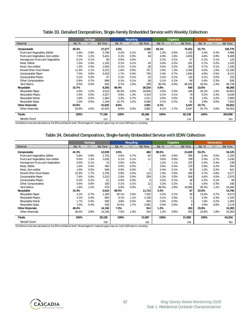
82 King County Waste Monitoring 2018 Task 1: Residential Curbside Characterization
Table 33. Detailed Composition, Single-family Embedded Service with Weekly Collection
Table 34. Detailed Composition, Single-family Embedded Service with EOW Collection
Garbage Recycling Organics Generation Material Est. % + / - Est Tons Est. % + / - Est Tons Est. % + / - Est Tons Est. % + / - Est Tons
Compostable 35.3% 27,277 4.5% 2,050 93.1% 76,451 51.7% 105,778 Fruits and Vegetables, Edible 4.9% 0.9% 3,799 0.2% 0.1% 86 1.3% 0.5% 1,102 2.4% 0.4% 4,986 Fruits and Vegetables, Non-edible 7.0% 1.2% 5,431 0.1% 0.0% 34 4.9% 1.6% 4,004 4.6% 0.8% 9,469 Homegrown Fruits and Vegetables 0.1% 0.1% 58 0.0% 0.0% - 0.1% 0.1% 67 0.1% 0.1% 125 Meat, Edible 1.5% 0.4% 1,192 0.1% 0.1% 49 0.4% 0.2% 291 0.7% 0.2% 1,533 Meat, Non-edible 1.3% 0.3% 1,004 0.1% 0.1% 38 0.5% 0.2% 393 0.7% 0.1% 1,435 Mixed/Other Food Waste 11.9% 2.1% 9,223 1.6% 0.9% 707 2.9% 1.3% 2,400 6.0% 1.0% 12,330 Compostable Paper 7.0% 0.9% 5,423 1.7% 0.4% 755 2.4% 0.7% 1,944 4.0% 0.5% 8,121 Compostable Plastic 0.1% 0.0% 47 0.1% 0.1% 43 0.2% 0.1% 125 0.1% 0.0% 215 Other Compostables 0.9% 0.7% 698 0.1% 0.1% 38 0.1% 0.1% 99 0.4% 0.3% 835 Yard Debris 0.5% 0.3% 403 0.7% 1.0% 299 80.4% 6.0% 66,026 32.6% 2.4% 66,728
Recyclable 10.7% 8,293 86.9% 39,334 0.8% 640 23.6% 48,268 Recyclable Paper 4.6% 1.0% 3,513 59.3% 4.0% 26,845 0.5% 0.4% 446 15.1% 1.0% 30,803 Recyclable Plastic 2.9% 0.5% 2,257 9.5% 1.3% 4,310 0.1% 0.1% 79 3.2% 0.3% 6,646 Recyclable Metal 1.8% 0.5% 1,364 3.3% 0.7% 1,511 0.0% 0.0% 25 1.4% 0.2% 2,899 Recyclable Glass 1.5% 0.5% 1,159 14.7% 2.2% 6,669 0.1% 0.2% 91 3.9% 0.5% 7,919
Other Materials 53.9% 41,625 8.6% 3,881 6.1% 5,047 24.7% 50,553 Other Materials 53.9% 4.6% 41,625 8.6% 3.0% 3,881 6.1% 4.7% 5,047 24.7% 2.6% 50,553
Totals 100% 77,195 100% 45,266 100% 82,138 100% 204,599Sample Count 212 190 119 521
Confidence intervals calculated at the 90% confidence level. Percentages for material types may not total 100% due to rounding.
Garbage Recycling Organics Generation Material Est. % + / - Est Tons Est. % + / - Est Tons Est. % + / - Est Tons Est. % + / - Est Tons
Compostable 41.3% 12,038 3.5% 460 98.5% 21,628 53.2% 34,125 Fruits and Vegetables, Edible 5.8% 0.9% 1,703 0.5% 0.7% 62 1.8% 0.6% 395 3.4% 0.5% 2,160 Fruits and Vegetables, Non-edible 9.0% 1.3% 2,630 0.1% 0.1% 11 3.6% 0.9% 789 5.3% 0.7% 3,430 Homegrown Fruits and Vegetables 0.0% 0.1% 13 0.0% 0.0% - 1.0% 1.1% 225 0.4% 0.4% 238 Meat, Edible 1.6% 0.4% 464 0.0% 0.0% - 0.6% 0.4% 129 0.9% 0.2% 594 Meat, Non-edible 1.9% 0.5% 548 0.0% 0.0% 3 0.4% 0.1% 90 1.0% 0.2% 641 Mixed/Other Food Waste 12.9% 1.7% 3,756 0.9% 0.4% 112 1.9% 0.5% 409 6.7% 0.8% 4,277 Compostable Paper 7.6% 0.9% 2,210 2.0% 0.5% 259 2.3% 0.5% 506 4.6% 0.5% 2,975 Compostable Plastic 0.2% 0.2% 51 0.0% 0.0% 0 0.2% 0.1% 48 0.2% 0.1% 99 Other Compostables 0.6% 0.6% 183 0.1% 0.1% 12 0.2% 0.2% 51 0.4% 0.3% 246 Yard Debris 1.6% 1.2% 479 0.0% 0.0% 1 86.5% 2.8% 18,986 30.3% 1.1% 19,466
Recyclable 10.3% 3,016 89.5% 11,713 0.3% 67 23.0% 14,796 Recyclable Paper 4.1% 0.7% 1,185 56.1% 3.0% 7,342 0.2% 0.1% 46 13.4% 0.7% 8,573 Recyclable Plastic 3.1% 0.4% 894 9.1% 1.1% 1,196 0.1% 0.0% 11 3.3% 0.3% 2,100 Recyclable Metal 1.7% 0.4% 508 3.8% 0.5% 494 0.0% 0.0% 3 1.6% 0.2% 1,004 Recyclable Glass 1.5% 0.4% 430 20.5% 2.7% 2,681 0.0% 0.0% 8 4.9% 0.6% 3,119
Other Materials 48.4% 14,106 7.0% 914 1.2% 263 23.8% 15,283 Other Materials 48.4% 3.8% 14,106 7.0% 1.4% 914 1.2% 0.8% 263 23.8% 1.8% 15,283
Totals 100% 29,159 100% 13,087 100% 21,958 100% 64,204Sample Count 239 165 158 562
Confidence intervals calculated at the 90% confidence level. Percentages for material types may not total 100% due to rounding.
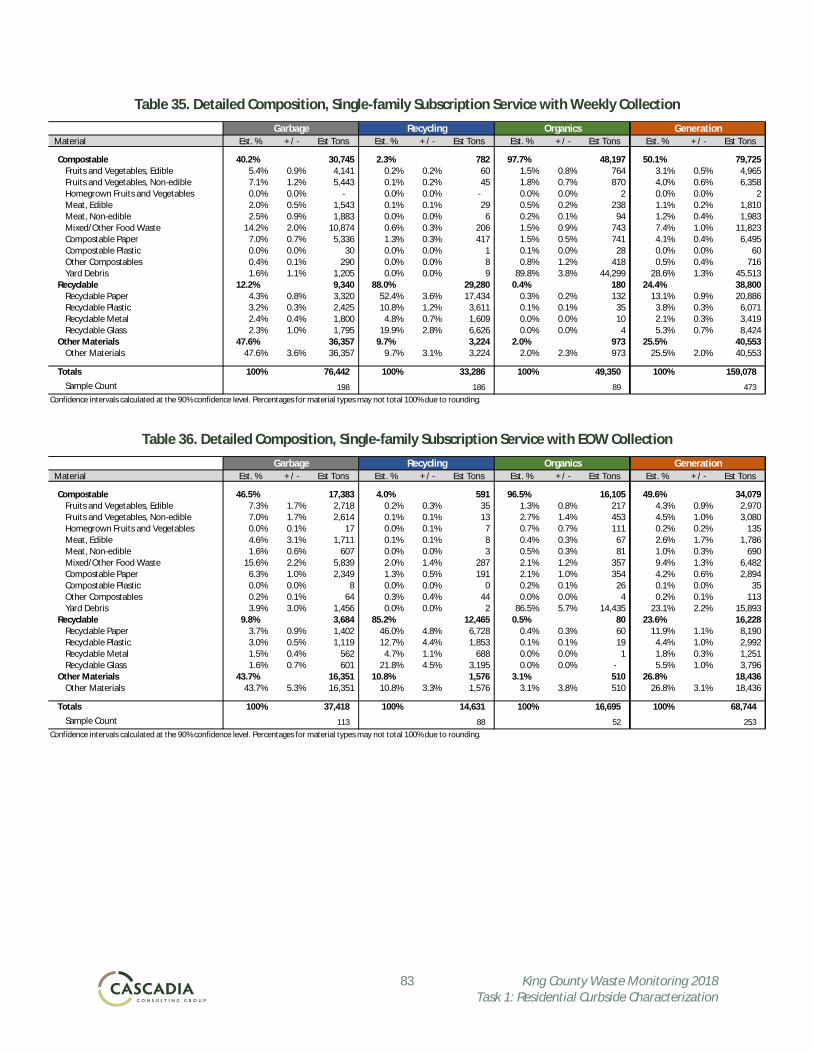
83 King County Waste Monitoring 2018 Task 1: Residential Curbside Characterization
Table 35. Detailed Composition, Single-family Subscription Service with Weekly Collection
Table 36. Detailed Composition, Single-family Subscription Service with EOW Collection
Garbage Recycling Organics Generation Material Est. % + / - Est Tons Est. % + / - Est Tons Est. % + / - Est Tons Est. % + / - Est Tons
Compostable 40.2% 30,745 2.3% 782 97.7% 48,197 50.1% 79,725 Fruits and Vegetables, Edible 5.4% 0.9% 4,141 0.2% 0.2% 60 1.5% 0.8% 764 3.1% 0.5% 4,965 Fruits and Vegetables, Non-edible 7.1% 1.2% 5,443 0.1% 0.2% 45 1.8% 0.7% 870 4.0% 0.6% 6,358 Homegrown Fruits and Vegetables 0.0% 0.0% - 0.0% 0.0% - 0.0% 0.0% 2 0.0% 0.0% 2 Meat, Edible 2.0% 0.5% 1,543 0.1% 0.1% 29 0.5% 0.2% 238 1.1% 0.2% 1,810 Meat, Non-edible 2.5% 0.9% 1,883 0.0% 0.0% 6 0.2% 0.1% 94 1.2% 0.4% 1,983 Mixed/Other Food Waste 14.2% 2.0% 10,874 0.6% 0.3% 206 1.5% 0.9% 743 7.4% 1.0% 11,823 Compostable Paper 7.0% 0.7% 5,336 1.3% 0.3% 417 1.5% 0.5% 741 4.1% 0.4% 6,495 Compostable Plastic 0.0% 0.0% 30 0.0% 0.0% 1 0.1% 0.0% 28 0.0% 0.0% 60 Other Compostables 0.4% 0.1% 290 0.0% 0.0% 8 0.8% 1.2% 418 0.5% 0.4% 716 Yard Debris 1.6% 1.1% 1,205 0.0% 0.0% 9 89.8% 3.8% 44,299 28.6% 1.3% 45,513
Recyclable 12.2% 9,340 88.0% 29,280 0.4% 180 24.4% 38,800 Recyclable Paper 4.3% 0.8% 3,320 52.4% 3.6% 17,434 0.3% 0.2% 132 13.1% 0.9% 20,886 Recyclable Plastic 3.2% 0.3% 2,425 10.8% 1.2% 3,611 0.1% 0.1% 35 3.8% 0.3% 6,071 Recyclable Metal 2.4% 0.4% 1,800 4.8% 0.7% 1,609 0.0% 0.0% 10 2.1% 0.3% 3,419 Recyclable Glass 2.3% 1.0% 1,795 19.9% 2.8% 6,626 0.0% 0.0% 4 5.3% 0.7% 8,424
Other Materials 47.6% 36,357 9.7% 3,224 2.0% 973 25.5% 40,553 Other Materials 47.6% 3.6% 36,357 9.7% 3.1% 3,224 2.0% 2.3% 973 25.5% 2.0% 40,553
Totals 100% 76,442 100% 33,286 100% 49,350 100% 159,078Sample Count 198 186 89 473
Confidence intervals calculated at the 90% confidence level. Percentages for material types may not total 100% due to rounding.
Garbage Recycling Organics Generation Material Est. % + / - Est Tons Est. % + / - Est Tons Est. % + / - Est Tons Est. % + / - Est Tons
Compostable 46.5% 17,383 4.0% 591 96.5% 16,105 49.6% 34,079 Fruits and Vegetables, Edible 7.3% 1.7% 2,718 0.2% 0.3% 35 1.3% 0.8% 217 4.3% 0.9% 2,970 Fruits and Vegetables, Non-edible 7.0% 1.7% 2,614 0.1% 0.1% 13 2.7% 1.4% 453 4.5% 1.0% 3,080 Homegrown Fruits and Vegetables 0.0% 0.1% 17 0.0% 0.1% 7 0.7% 0.7% 111 0.2% 0.2% 135 Meat, Edible 4.6% 3.1% 1,711 0.1% 0.1% 8 0.4% 0.3% 67 2.6% 1.7% 1,786 Meat, Non-edible 1.6% 0.6% 607 0.0% 0.0% 3 0.5% 0.3% 81 1.0% 0.3% 690 Mixed/Other Food Waste 15.6% 2.2% 5,839 2.0% 1.4% 287 2.1% 1.2% 357 9.4% 1.3% 6,482 Compostable Paper 6.3% 1.0% 2,349 1.3% 0.5% 191 2.1% 1.0% 354 4.2% 0.6% 2,894 Compostable Plastic 0.0% 0.0% 8 0.0% 0.0% 0 0.2% 0.1% 26 0.1% 0.0% 35 Other Compostables 0.2% 0.1% 64 0.3% 0.4% 44 0.0% 0.0% 4 0.2% 0.1% 113 Yard Debris 3.9% 3.0% 1,456 0.0% 0.0% 2 86.5% 5.7% 14,435 23.1% 2.2% 15,893
Recyclable 9.8% 3,684 85.2% 12,465 0.5% 80 23.6% 16,228 Recyclable Paper 3.7% 0.9% 1,402 46.0% 4.8% 6,728 0.4% 0.3% 60 11.9% 1.1% 8,190 Recyclable Plastic 3.0% 0.5% 1,119 12.7% 4.4% 1,853 0.1% 0.1% 19 4.4% 1.0% 2,992 Recyclable Metal 1.5% 0.4% 562 4.7% 1.1% 688 0.0% 0.0% 1 1.8% 0.3% 1,251 Recyclable Glass 1.6% 0.7% 601 21.8% 4.5% 3,195 0.0% 0.0% - 5.5% 1.0% 3,796
Other Materials 43.7% 16,351 10.8% 1,576 3.1% 510 26.8% 18,436 Other Materials 43.7% 5.3% 16,351 10.8% 3.3% 1,576 3.1% 3.8% 510 26.8% 3.1% 18,436
Totals 100% 37,418 100% 14,631 100% 16,695 100% 68,744Sample Count 113 88 52 253
Confidence intervals calculated at the 90% confidence level. Percentages for material types may not total 100% due to rounding.