residential microgrids for disaster recovery operations ... · 7 transient-simulation scenarios and...

i

Residential Microgrids for Disaster Recovery Operations

James W. Hurtt

Thesis submitted to the Faculty of the

Virginia Polytechnic Institute and State University

in partial fulfillment of the requirements for the degree of

Master of Science

in

Electrical Engineering

Lamine Mili, Chair

Jason Lai

C. Yaman Evrenosoglu

November 15, 2012

Falls Church, Virginia

Keywords: Microgrids, Distributed Generation, Modeling, Disaster Recovery

© Copyright 2012, James Hurtt

ii

Abstract

The need for a continuous supply of electric power is vital to providing the basic services of

modern life. The energy infrastructure that the vast majority of the world depends on, while very

reliable, is also very vulnerable. This infrastructure is particularly vulnerable to disruptions

caused by natural disasters. Interruptions of electric service can bring an end to virtually all the

basic services that people are dependent on. Recent natural disasters have highlighted the

vulnerabilities of large, economically developed, regions to disruptions to their supply of

electricity. The widespread devastation from the 2011 Japanese Tsunami and Hurricane Irene in

North America, have demonstrated both the vulnerability of the contemporary power grids to

long term interruption of service and also the potential of microgrids to ride through these

interruptions. Microgrids can be used before, during, and after a major natural disaster to supply

electricity, after the main grid source has been interrupted. This thesis researches the potential of

clean energy microgrids for disaster recovery. Also a model of a proposed residential microgrid

for transient analysis is developed. As the world demands more energy at increasingly higher

levels of reliability, the role of microgrids is expected to grow aggressively to meet these new

requirements. This thesis will look at one potential application for a microgrid in a residential

community for the purpose of operating in an independent island mode operation.

iii

Acknowledgements

I would first like to thank my friends, family, and colleagues for giving support over the years to

reach this level of academic achievement. In particular, my wife Anna, who has been an endless

source of strength and encouragement. As well as my parents who have nurtured me from a

young age to be hard working and be curious. My brother, for always being there and always

knowing more about the world than I ever will. I am especially grateful for my colleagues at

work who have given me the support I needed to work and achieve my academic goals

simultaneously. A special thanks to the late Louis Larkin, for whom I worked with for many

years. He taught me the value of engineering excellence.

My development as a researcher would not be possible without the support of my advisor, Dr.

Lamine Mili. His guidance and patience with me as my thesis slipped further behind schedule is

much appreciated. I am also very grateful for my committee members Dr. Lai and Dr.

Evrenosoglu for agreeing to sit on my committee and giving me very constructive feedback.

Finally, I would like to acknowledge my good friend, Ibrahima Diagne. Ibrahima has been an

invaluable friend and colleague over the past several years. He has helped me out on numerous

occasions. I would not be where I am today without his support. Thank you.

This thesis is dedicated to my son Daniel.

iv

Contents

1 Research Introduction ……………………………………………………………............... 1

1.1 Microgrid Definition .......................................................................................................... 2

1.2 Research Motivation …………………………………………………………….............. 3

1.3 Microgrid Concept and Scope of Study …………………………………………............. 4

1.4 Contributions ……………………………………………………………………............. 6

1.5 Thesis Overview ………………………………………………………………………… 6

2 Literature Review ………………………………………………………………………….. 8

2.1 Microgrid History ……………………………………………………………………….. 9

2.2 Microgrids in Contemporary Application ……………………………………………… 11

2.2.1 Microgrids for Disaster Recovery ……………………………………………… 11

2.3 Clean Energy and Fuel Independent Microgrids …………………………………......... 12

2.4 Trends in Microgrid Research and Development ……………………………………… 13

3 Hurricane Occurrence and Impact ……………………………………………………… 14

3.1 Brief Overview of Atlantic Hurricanes ………………………………………………… 14

3.2 Hurricane Impact to Electricity Delivery ………………………………………………. 16

3.2.1 Case Studies: Katrina, Wilma, Ike ……………………………………………... 16

3.2.1.1 Hurricane Katrina ………………………………………………………. 17

3.2.1.2 Hurricane Wilma ……………………………………………………….. 18

3.2.1.3 Hurricane Ike …………………………………………………………... 19

3.2.2 Summary of Case Studies ……………………………………………………… 19

4 Modeling Overview………………………………………………………………………... 21

4.1 Environmental Characteristics Model ………………………………………………….. 21

4.1.1 Wind Resource Environmental Model ……………………………………......... 21

4.1.2 Solar Resource Environmental Model …………………………………………. 24

4.2 Battery Storage Model …………………………………………………………………. 26

4.2.1 Battery Voltage Source Model …………………………………………………. 27

4.2.2 Battery Array Model and Implementation ……………………………………... 30

4.2.3 PSCAD Implementation and Verification ……………………………………... 32

4.3 Photovoltaic (PV) Model ………………………………………………………………. 35

4.3.1 Current Source Diode Model …………………………………………………... 35

4.3.2 Photovoltaic Sizing …………………………………………………………….. 39


4.4 Wind Turbine Model …………………………………………………………………… 45

4.4.1 Wind Turbine Transient Model ………………………………………………... 46

4.4.1.1 Wind Turbine Approximate Model ……………………………………. 46

4.4.1.2 Permanent Magnet Machine Model ……………………………………. 48

4.4.1.3 Three Phase Rectifier Model …………………………………………... 49


4.5 Residential Load Model ………………………………………………………………... 55

5 Microgrid Control System ……………………………………………………………….. 60

5.1 Concept of Operation ………………………………………………………………….. 60

5.2 Inverter Model …………………………………………………………………………. 63

5.2.1 Inverter Design …………………………………………………………………. 63

v

5.2.2 LC Filter Design ……………………………………………………………….. 66

5.2.3 Inverter PQ Controller …………………………………………………………. 68

5.2.4 PSCAD Implementation ……………………………………………………….. 72

5.3 Power Management Controller ………………………………………………………… 75

5.3.1 Island Mode Power Flow Balancing …………………………………………… 77

5.3.2 Environmental Resource Monitor ……………………………………………… 78

5.3.3 Emergency Load Control ………………………………………………………. 79

5.4 Island-mode Droop Control ……………………………………………………………. 80

6 Integrated Microgrid Model and Steady-State Verification Results ………………….. 84

6.1 Microgrid Implementation in PSCAD …………………………………………………. 84

6.1.1 Transformer and Line-Loss Consolidation …………………………………….. 84

6.1.2 PSCAD Microgrid Model ……………………………………………………… 85

6.2 Microgrid Steady-State Performance ………………………………………………….. 86

6.2.1 Grid-Connected Steady-State Operation ………………………………………. 86

6.2.2 Island-Mode Steady-State Operation ………………………………………….. 88

7 Transient-Simulation Scenarios and Results …………………………………………… 91

7.1 Scenario 1: Loss of Grid, Transition to Island Mode Operation ………………………. 92

7.2 Scenario 2: Island Mode - Interconnecting PV Microsources …………………………. 94

7.3 Scenario 3: Island Mode Operation-Variability of Microsources

with a Constant Load …………………………………………………………………... 99

7.4 Scenario 4: Island Mode-Wind Gust Ride Through ………………………………….. 102

7.5 Scenario 5: Island Mode-PMC Battery Management ………………………………… 105

7.6 Scenario 6: Island Mode-PMC Source Curtailment ………………………………….. 107

7.7 Scenario 7: Island Mode-Wind Turbine Fault Isolation ……………………………… 110

7.8 Scenario 8: Microgrid Resynchronization with the Grid ……………………………... 113

8 Conclusions and Future Work ………………………………………………………….. 116

8.1 Research Summary …………………………………………………………………… 116

8.2 Recommended Future Work ………………………………………………………….. 117

8.2.1 Communications Future Work ………………………………………………... 117

8.2.2 Controller Future Work ……………………………………………………….. 116

8.2.3 Economic Analysis Future Work ……………………………………………... 118

8.2.4 Proposed Pilot Implementation ………………………………………………. 119

References ……………………………………………………………………………………. 120

vi

List of Figures

1.1: Microgrid Concept for Residential Distribution ……………………………………. 3

1.2: Conceptualization of Proposed Residential Microgrid ……………………………... 4

1.3: One-line Diagram for the Single Phase Microgrid …………………………………. 5

2.1: Microgrid Concept for Remote Military Installations …………………………….. 10

2.2: Microgrid Megawatt Capacity Growth Projections ……………………………….. 13

3.1: Hurricane Cyclone Formation …………………………………………………….. 15

3.2: Major Landfall Hurricanes in 2005 and 2008 …………………………………….. 16

3.3: New Orleans and Surrounding Vicinity Power Outage Map ……………………... 18

3.4: Power Outage Map in the Houston Metro ………………………………………… 19

3.5: Number of Customers Without Power vs. Number of Weeks Since Landfall ……. 20

4.1: Annual Average Wind Resource for the State of Florida …………………………. 22

4.2: Average South Florida Wind Speed Sample Near Sea-Level …………………….. 23

4.3: Average South Florida Wind Speed Sample at 30 feet Height ……………………. 24

4.4: Average Solar Energy Resource for the Continental United States ………………. 25

4.5: Average Hourly Solar Irradiation for September in South Florida ……………….. 26

4.6: Typical Battery Discharge Curve of a 1.2 V Lead Acid Cell ……………………... 28

4.7: Equivalent circuit of a battery cell ………………………………………………… 30

4.8: PSCAD Implementation of the Battery Model Control …………………………… 33

4.9: PSCAD Implementation of Battery System Equivalent Circuit …………………... 33

4.10: Response of Battery System from Discharging to Charging State ………………. 34

4.11: Battery System Efficiency at Nominal Discharge ……………………………….. 34

4.12: The I-V curve for a BP 220 Watt module ………………………………………... 35

4.13: PV cell equivalent circuit model …………………………………………………. 36

4.14: PV Array Equivalent Circuit Implemented in PSCAD ………………………….. 41

4.15: Calculation of the Maximum Power Point Implemented in PSCAD ……………. 41

4.16: Short Circuit Current and Open Circuit Voltage Calculation in PSCAD ………... 42

4.17: Fill Factor Calculation for the PV Array ………………………………………… 42

4.18: Calculation of the Series and Shunt Resistance of the PV Array ………………... 43

4.19: The Power Output Response to a Change in Solar Irradiance …………………... 44

4.20: Efficiency of the PV Array System (Includes Inverter Losses) …………………. 44

4.21: Block Diagram of the Wind Turbine Transient Model ………………………….. 45

4.22: The Power Curve of the Hummer Power Unit …………………………………... 48

4.23: The Effect of a 3-Phase Full Wave Rectifier …………………………………….. 50

4.24: Wind Turbine Approximation Model ……………………………………………. 52

4.25: Existing PSCAD PM Machine Model …………………………………………… 52

4.26: 3-Phase Rectifier Bridge for Wind Turbine Model ……………………………… 53

4.27: Wind Turbine Response to a Change in Wind Speed ……………………………. 54

4.28: Efficiency of the Wind turbine System (Includes Mechanical, Generator, Rectifier,

and Inverter Losses) ……………………………………………………………………. 55

4.29: Hourly Energy Consumption Profile of a Standard Home and Home with PV and

High Efficiency Appliances ……………………………………………………………. 56

4.30: Hourly Demand Curve for High Efficiency Microgrid Home …………………... 57

4.31: Single Residence Average Hourly Generation and Demand Profile …………….. 58

4.32: Total Average Energy Generated and Consumed in a Single Residence ………... 59

vii

5.1: Top-Level Controller Hierarchy …………………………………………………... 61

5.2: Microgrid Operation and Reference Points ……………………………………….. 62

5.3: Battery Inverter Control Concept of Operation …………………………………… 62

5.4: H-Bridge Inverter with Filtering and Grid Connection …………………………… 63

5.5: Power Semiconductor Capability Chart …………………………………………... 65

5.6: General Control Loop for Real Power Control ……………………………………. 70

5.7: General Control Loop for Reactive Power Control ……………………………….. 70

5.8: PWM Train Generated from Carrier Signal ………………………………………. 71

5.9: PWM Generator for PQ Controller ……………………………………………….. 72

5.10: H-Bridge, LC Filter, and Isolation Transformer for the Inverter Circuit ………... 72

5.11: Control Loop for Real Power/Angle Control ……………………………………. 73

5.12: Control Loop for Reactive Power/Voltage Control ……………………………… 73

5.13: Verification of Voltage Output from the Inverter against Grid Voltage ………… 74

5.14: Currrent Harmonic Spectrum for Inverter at Full Load …………………………. 74

5.15: Voltage Harmonic Spectrum for Inverter at Full Load ………………………….. 75

5.16: PMC Top-Level Control Diagram ……………………………………………….. 76

5.17: Power Balancing Function Implementation in PSCAD …………………………. 78

5.18: Wind/Solar Resource Monitor Implementation in PSCAD ……………………… 79

5.19: PMC Emergency Load Control Implementation in PSCAD …………………….. 80

5.20: Droop Characteristics for Frequency and Voltage ………………………………. 81

5.21: Droop Controller Implementation for Phase Control on the Battery Inverter …… 82

5.22: Droop Controller Implementation for Voltage Control on the Battery Inverter …. 82

5.23: Voltage Transient Response with Droop Control ………………………………... 83

5.24: Phase Transient Response with Droop Control ………………………………….. 83

6.1: Microgrid Implemented in PSCAD ……………………………………………….. 85

6.2: Grid Connected Steady State Power ………………………………………………. 87

6.3: Grid Connected Steady State Voltage …………………………………………….. 87

6.4: Grid Connected Steady State Frequency ………………………………………….. 88

6.5: Island Mode Steady State Power ………………………………………………….. 89

6.6: Island Mode Steady State Voltage ………………………………………………… 89

6.7: Island Mode Steady State Frequency ……………………………………………… 90

7.1: One-line Diagram of the Microgrid with Measurement Points …………………… 92

7.2: Power Load Demand and Supply from PV, Batt, and WTG ……………………… 95

7.3: System Voltages for the Common Bus, Residence Bus, and Battery Bus ………... 94

7.4: Battery Phase Angle Change (w.r.t. to Residence Bus) …………………………… 95

7.5: System Frequency Response during Transition …………………………………… 95

7.6: Change in Power Output during Transition ……………………………………….. 97

7.7: Change in PV and Battery Output during Transition ……………………………... 97

7.8: Voltage Response during Transition ……………………………………………… 98

7.9: Frequency Response during Transition …………………………………………… 98

7.10: Battery Phase Angle (w.r.t. to Load Bus) during Transition …………………….. 99

7.11: Worst Case Solar Irradiance Variation Frequency ……………………………... 100

7.12: Worst Case Wind Speed Variation Frequency …………………………………. 100

7.13: Power Output Resulting From Resource Variation …………………………….. 101

7.14: Voltage Response to Changing Renewable Sources Variation ………………… 101

7.15: Battery Phase Angle Response to Changing Renewable Sources Output ……… 102

viii

7.16: Worst Case Wind Gust …………………………………………………………. 104

7.17: Power Output during Wind Gust ……………………………………………….. 104

7.18: Power Output during Wind Gust ……………………………………………….. 105

7.19: Battery Phase Angle Response during Wind Gust ……………………………... 105

7.20: Worst Case Battery Discharge Rate …………………………………………….. 106

7.21: PMC Reducing Curtailing Demand from Residences during

Battery Discharge ……………………………………………………………….. 107

7.22: Battery Phase Angle Response to Rapid Discharging ………………………….. 107

7.23: PMC Source Curtailment Due to High Battery SOC …………………………... 108

7.24: WTG 1 Breaker Initialized by PMC ……………………………………………. 109

7.25: Battery SOC Change during Curtailment ………………………………………. 109

7.26: Battery SOC Change during Curtailment ………………………………………. 110

7.27: Battery and WT Contribution to Fault Event …………………………………… 111

7.28: System Voltage Response to Fault Event ………………………………………. 112

7.29: WTG Inverter Fault Current Contribution and Isolation (after 3 cycles) …….… 112

7.30: WTG PM Generator Fault Current Contribution

and Isolation (after 3 cycles) ……………………………………………………. 112

7.31: Change in Power Output during Resynchronization …………………………… 114

7.32: System Voltage Change during Resynchronization ……………………………. 114

7.33: Battery Phase Angle Change during Resynchronization ………………….......... 115

ix

List of Tables

3.1: Electrical Infrastructure Impact from Major Hurricanes ………………………….. 20

4.1: Electrical Characteristics of the BP 3220 Panel …………………………………... 39

5.1: Inverter Hardware Specification …………………………………………………... 65

5.2: LC Filter Specification …………………………………………………………….. 68

5.3: Truth Table for the H-Bridge Inverter …………………………………………….. 71

5.4: PMC Load Balancing Truth Table ………………………………………………… 76

6.1: Grid-Connected Mode Steady State Operation Unit Status ……………………….. 86

6.2: Island Mode Steady State Operation Unit Status ………………………………….. 88

7.1: System Configuration for Scenario 1 ……………………………………………… 93

7.2: System Configuration for Scenario 2 ……………………………………………… 96

7.3: System Configuration for Scenario 3 …………………………………………….. 100





7.8: System Configuration for Scenario 8 ….................................................................. 113

1

Chapter 1

Research Introduction

Natural disasters have a devastating impact on people, the environment, and everyday way of

life. Virtually no place on earth is spared from natural disasters such as floods, hurricanes,

earthquakes, tsunami’s, drought, tornados, blizzards, and many other events. On the southeastern

seaboard of the United States, the primary threat is from hurricanes. In particular, the state of

Florida bears the brunt of many tropical systems. Between the years 1851-2004, 110 hurricanes

impacted the state [1]. This accounted for 40% of all hurricanes that have struck the eastern

seaboard of the United States during that time [1]. By the same margins, 35 major hurricanes

(category 3 and higher) have made landfall during this time in Florida [1]. Hurricane impacts

often result in extensive damage to local infrastructure. Electric service can quickly be

interrupted for millions of customers and in some cases, remain offline for weeks afterwards [2].

The growing development of microgrids has the potential to provide continuous power to these

affected communities during an outage of indefinite duration. Currently, a large number of

residences use emergency gasoline/diesel generators during outages. Drawbacks to the current

implementation of these generators are that they are isolated, typically non-redundant, produce

dangerous emissions, and are dependent on a large fuel supply during extended outages. The

safety concerns with emergency generators are of particular concern. According to [3], between

1999-2011, 755 people died in the United States from carbon monoxide poisoning from

emergency generators. Microgrids with “green” sources of energy generation can reduce

dependence on these gas generators while reducing emissions without heavy reliance on

inefficient emergency gasoline generators. Another consideration is the large number of injuries

2

that occur after a hurricane has past that are related to improper use and handling of gasoline

generators with injuries ranging from electric shock, carbon monoxide poisoning, and physical

injury. From this, it can be seen how an autonomous microgrid can provide additional safety

over existing technology.

1.1 Microgrid Definition

Microgrids have the potential to drastically alter the infrastructure and nature of power

generation on a global scale. While the formal definition of a microgrid varies by audience, a

common definition is an integrated energy system consisting of distributed energy resources and

multiple electrical loads operating as a single, autonomous grid either in parallel to or “islanded”

from the existing utility power grid [4]. The key distinguishing feature between a microgrid and

the classical macrogrid is the collocation of generation and load centers. The network minimizes

the burden of large transmission and distribution networks. Only a small, local, distribution

system is needed to interconnect generation and load centers. Figure 1.1 shows a conceptual

architecture for a microgrid, intertie with an existing radial distribution system.

3

Figure 1.1: Microgrid Concept for Residential Distribution [5]

1.2 Research Motivation

The primary motivation for pursuing this research topic is to highlight the key features that a

microgrid can provide to power system networks that the contemporary electric grid cannot

achieve. This includes greater reliability, resilience, emissions reduction, and rapid demand

management. In particular, in the event of large scale natural disasters, the limitations of the

existing grid are apparent. Dependence on high voltage transmission and distribution lines,

predominantly routed overhead, often result in widespread outages during and immediately

following a natural disaster. Customers in small towns and rural areas are generally given lower

priority to restoring service than the population centers in larger cities. Customers without

emergency generators or inadequate fuel supplies, face a prolonged outage. This research will

4

emphasize clean and sustainable microgrids as an alternative to the traditional emergency

gasoline generators. The robustness of the system to transients that occur during and after a

storm will also be evaluated.

1.3 Microgrid Concept and Scope of Study

The concept for this microgrid is 3 small residences, adjacent to each other, with renewable

sources installed on each property. One wind turbine and one PV array is connected to each

residence. The residences are tied back to a local substation on a single phase where they connect

to the local distribution substation. A battery storage bank is tied in to the substation at another

location to provide backup for the renewable devices. A notional concept for the microgrid is

captured using Google sketch-up and shown in Figure 1.2.

Figure 1.2: Conceptualization of Proposed Residential Microgrid

It can be seen that the proposed microgrid fits within the boundaries of the referenced residence

without an excessive amount of real estate required. In a practical system, the turbine would

likely be located further away from the residences to provided better airflow around the blades,

PV Array

Solar Heater

Wind Turbine

Batt Array

5

but this is shown for visualization purposes. The residences are tied to the same single phase

feeder from the residential distribution source. It is also assumed that a small amount of real

estate is required for the battery storage module shown in Figure 1.2. The details of the physical

layout are not covered in this thesis, but rather notionally given as a reference to the feasibility of

the proposed microgrid. The one-line diagram for the microgrid is shown in Figure 1.3. This one-

line is not representative of all residential distribution layouts. There are numerous variations of

residential distribution schemes that exist.

Figure 1.3: One-line Diagram for the Single Phase Microgrid

While the proposed model is limited to 3 residences and a small number of generation sources, it

is important to note that this system is highly scalable. The size of the microgrid for this research

is limited to reduce simulation time and provided more detailed results for a smaller network.

Future study into this system should consider a much larger number of nodes and is proposed in

Chapter 8. The proposed system can be implemented in a variety of network schemes that do not

6

alter the operation of the microgrid. The operation of the system is focused on island mode

generation and maintaining voltage and frequency stability with the residences. Grid-connected

mode is investigated for steady-state verification, as well as disconnecting and reconnecting to

the macrogrid, but is not the emphasis of this research. Scenarios to be investigated will be

focused on changing system conditions and how the microgrid responds.

1.4 Contributions

This research proposes a novel microgrid that is capable of being islanded from the main grid

and free of fuel source generations (namely gas generators and/or fuel cells). While significant

research is being performed in microgrids and disaster recovery currently (see Chapter 2), there

is limited research on microgrid systems for clean, sustainable electricity delivery. This novel

system architecture also produces novel solutions for power flow and system stability. The

constraints of this novel approach also leads to new challenges. For instance, control of power

output through phase angle droop control, rather than classical frequency control, is presented in

this research. Utilizing a battery array, rather than fossil system, for a reference point and for

stabilizing the microgrid power production is also discussed. Novel modeling and control

schemes for an islanded microgrid are also presented that allow for greater energy utilization and

demand side management. This work sets the foundation for further investigation and

implementation for future research studies.

1.5 Thesis Overview

This thesis is divided into 8 chapters. Chapter 1 provides an introduction to the topic and the

scope of the research. Chapter 2 covers the literature review of previous research efforts and

7

similar efforts performed on microgrid research. Chapter 3 provides motivation for this specific

research topic through reviewing hurricanes and impact on electric power delivery. Chapter 4

covers in detail the various sub-models that make up the generation sources, environmental

model, and residential loads. Chapter 5 goes over the control system and hierarchy of the

microgrid. Chapter 6 covers the interconnection of the sub-models from chapter 4 and control

system from chapter 5 together into an integration microgrid model along with steady state

results. Chapter 7 covers the results of various dynamic scenarios for the consolidated microgrid.

Chapter 8 concludes the thesis with final results and recommendations for future expansion of

the research topic.

8

Chapter 2

Literature Review

Recent natural disasters such as the 2011 Japanese Tsunami and Hurricane Irene (U.S. 2011)

have demonstrated the potential of microgrids for disaster recovery. In particular, university

research microgrids have made their way into the spotlight after these two events. During the

Japanese tsunami, the city of Sendai, which is located on the Northeastern coast of Japan, was

directly in the path of the major tsunami [6]. Hundreds of residents perished as catastrophic

damage occurred to buildings and infrastructure as far as 8 miles inland [6]. One surprising

success story from this devastation, was the resilience of the Tohoku Fukushi University

microgrid. This system supplied 1 megawatt of uninterrupted power to the university buildings

and hospital for several days until power was restored [6]. Through a combination of fuel cells,

photovoltaic panels, and natural gas microturbines the university was able to keep the lights on

while much of the city was left in the dark. A similar operational success story occurred when

Hurricane Irene struck the U.S. Northeast coast in 2011 [7]. Three university microgrids located

at Cornell University (38 MW microgrid), New York University-Washington Square Park (13.4

MW), and Utica College (3.6 MW) were able to supply uninterrupted power immediately

following the storm [7]. Overall, interest in microgrids for emergency events is growing and

accelerating by each new natural disaster.

9

2.1 Microgrid History

Basic microgrids have been around since the early days of electrification. Early generation

facilities, such as Thomas Edison’s generating stations in New York City, were located very

close to customer lighting loads. These systems were isolated where a few string of lights would

intertie to a single generator. As demand for lighting grew and the advent of alternating current,

the nature of electricity changed. Generation units grew larger, more interconnected, and located

further away from load centers. Large scale transmission lines interconnected the electrical grids

of multiple utilities together. From this growing interconnection, the macrogrid was formed and

individual microgrids became uneconomical compared with the larger economy of scale

networks [4]. Microgrids have held on in some key markets over the years where connection to a

macrogrid was either unreliable or unavailable for local demand. These include remote

communities, factories with large industrial loads, and critical infrastructure (i.e. hospitals,

emergency responders, military installations, etc…) [4]. In particular, the U.S. Department of

Defense (DoD) has been on the forefront of recent microgrid development projects for remote

military bases. Microgrid technology for the defense industry is being driven by the need to

reduce fuel convoys to forward operating bases [8]. These convoys traverse very dangerous

remote regions with heavy casualties by military personnel and contractors. Figure 2.1 show a

proposed microgrid for defense application developed by the Lockheed Martin Corporation.

10

Figure 2.1: Microgrid Concept for Remote Military Installations [8]

While microgrids have found a niche in defense and critical infrastructure markets, they are also

growing in distributed generation as well. With increasing demand for electricity, competitive

electricity markets, and greater reliability concerns, they are making a significant comeback.

New projects offer isolated, clean, and reliable power production for an adjacent customer

demand. Most major commercial buildings are now equipped with some form of emergency

power, typically a diesel generator with a short duration battery backup system [9]. In addition,

numerous universities are investing in microgrids for research opportunities and to meet local

demand. Residential communities have the potential for multiple homes with distributed

resources attached to them to work in concert to deliver cost effective, reliable, energy to homes.

While the residential market for microgrids is currently just beginning to emerg, it does offer the

largest market potential for growth. New pilot projects for microgrids are being developed at

numerous research universities, like the 4 referenced in Chapter 1, as well national laboratories.

The national renewable energy laboratory (NREL) in Golden, CO is developing a test microgrid

to test the many variations of the system configuration that can be utilized [9]. This project along

11

with others signals a are large shift in research and new product development into the area of

microgrid development.

2.2 Microgrids in Contemporary Application

There are several power operations where microgrids have a practical application. Common

implementations include peak load shaving for demand side management. In this situation,

dispatchable units such as a diesel generators, microturbines, fuel cell stacks, or battery array

come online to supply part of the load to a customer distribution during periods of high demand

(which usually occurs during mid-afternoon hours). This implementation can offer cost

competitive power in a real time electricity pricing market. Another implementation is for

backing up the local distribution network when electricity from the local network in unreliable

(i.e. weak grid). In this application a variety of resources would be on standby, ready to pickup

instantaneous drops in supply from the macrogrid. This application is very desirable in remote

regions where local utilities cannot meet high electric reliability due to a number of reasons. In

this case, microgrids can backup local supply and provide residents with a higher reliability

source of electricity.

2.2.1 Microgrids for Disaster Recovery

One area of particular interest, and the basis of this thesis, are microgrids for disaster recovery

operations. In this situation, the microgrid must provide power to the entire electric load for an

indefinite period of time. In previous research, [10] and [11] proposed microgrids for disaster

recovery, looking at both probability of micro-source failures and modeling of controls. In [10] a

small system is proposed consisting of a doubly-fed induction wind generator and a small hydro-

12

power turbine. This paper looks at both the connection to and disconnection from the grid during

a disaster event. In [11] the authors investigate a significantly more complex microgrid with

multiple wind turbines, diesel generators, and battery storage array. In this paper, the reliability

of a microgrid during a disaster event is evaluated. Of principle importance is the ability to

maintain power supply to the customer when one or more units go offline. During a widespread

outage, damage to the microgrid infrastructure must also be considered. The robustness of the

microgrid from internal faults should also be considered.

2.3 Clean Energy and Fuel Independent Microgrids

There is limited research available on microgrids that do not use either a diesel generator or a

microturbine as the primary generation source. During a prolonged power outage, the risk of

generation units losing their fuel supply is very high. This can be partially mitigated by

maintaining a large emergency fuel supply, but this has its drawbacks. Difficulty in predicting

fuel supply needed presents a major risk in not having enough storage or having too much

storage (which can result in fuel quality degradation over time). There is also safety concerns

associated with storing vast quantities of fuel in regards to poisoning or risk of fire. A fuel

independent system eliminates the risks associated with fuel consumption and storage. There

have been research and pilot projects in clean energy microgrids, but they have not focused

explicitly on disaster recovery [12]. At the time of writing this thesis, there is limited research on

clean energy and fuel independent microgrids that have been proposed for disaster recovery.

13

2.4 Trends in Microgrid Research & Development

Interest in microgrids has grown substantially over the past decade. In addition to new and

innovative research efforts, a large number of projects are starting to come online. Pike’s

Research Group in Boulder, CO performs market research on the current state of microgrid

development and the expected growth in the future [13]. As indicated by Figure 2.2 below,

exponential growth in the microgrid market is expected over the next 4 years.

Figure 2.2: Microgrid Megawatt Capacity Growth Projections [13]

The aggressive projection has microgrids doubling in capacity every 2 years. Even the base

projection has them doubling in capacity every 3 years. As they continue to grow at a rapid pace,

so too will their capabilities. Increasing efficiency of small scale generation sources, better

power flow through power electronics, and more advanced communication are expected to drive

their increased development. This will lead to a greater expansion in the applications of

microgrids and the markets that they can be introduced into. The largest market potential is in

residential based systems, which is the focus of this thesis.

14

Chapter 3

Hurricane Occurrence and Impact

Prior to designing a microgrid that can meet this challenge, it is important to first briefly review

hurricanes and their historical impact on electric power delivery. The widespread devastation

caused by major hurricanes is the primary motivation for this thesis topic. Investigating the

implementation of a practical microgrid that can be utilized to maintain power delivery to a

residential demand during and after a major storm is very beneficial. With this motivation, the

design can move forward.

3.1 Brief Overview of Atlantic Hurricanes

Hurricanes (also known as typhoon and cyclones) are major storms that form over warm tropical

waters. They are characterized by strong winds and heavy rain in a self-sustaining spiraling

storm system. They are formed when the heat from vaporization of the warm tropical waters

creates a heat cycle, caused by the cooling of the water molecules as they rise in the air [14].

This result in cooler moisture being forced down and warm water vapor rising back up. When

this cycle becomes sustainable, strong winds form causing a rotational spiral [14]. As the storm

begins to move, it will strengthen as it continues pass over the warmer waters that provide

additional energy for the system. Figure 3.1 shows the anatomy of a self sustaining hurricane.

15

Figure 3.1: Hurricane Cyclone Formation [14]

When winds sustained up to 38 MPH classify the storm as a tropical depression, between 38 and

74 MPH is a classified as a tropical storm, and winds 75 MPH and higher are classified as a

hurricane [14]. The National Hurricane Center categorizes hurricanes on a scale of 1 to 5, based

off of sustained wind speed. Major hurricanes are those being category 3 or higher. In the

Northern Atlantic Ocean, hurricanes typically formed near the Cape Verde islands off the coast

of Western Africa. They can also form in the southern Gulf of Mexico [14]. These storms cause

the most significant damage to people and property when they make landfall. Figure 3.2 is a map

of the largest hurricanes that hit the United States in 2005 and 2008, which are the most

devastating in recent history [2].

16

Figure 3.2: Major Landfall Hurricanes in 2005 and 2008 [2]

3.2 Hurricane Impact to Electricity Delivery

The high winds and heavy rain from hurricanes often results in widespread power outages. The

major brunt of the damage is to overhead distribution lines that are taken out of service during

the storm due to trees, line pole failures, and debris that comes in contact with lines. Damage can

also occur to power plants, transmission lines, and substations. The duration of a power outage

can range from several hours to several weeks.

3.2.1 Case Studies: Katrina, Wilma, Ike

To further motivate research into microgrids for disaster recovery, a review of 3 major

hurricanes that previously occurred was performed. Hurricanes Katrina, Wilma, and Ike are

review in this section. These storms were particularly devastating to local infrastructure. In

17

particular, the level of power outages that occurred from each of these storms was very

widespread. They were also selected given their relatively recent history. Hurricane records go

back to the 1850’s, but only the past few years of storms have been selected to assess the impact

on power outages for contemporary power systems.

3.2.1.1 Hurricane Katrina

Hurricane Katrina was a major hurricane that hit large portions of Florida and the Gulf Coast

states in August, 2005. The storm peaked at category 5 rating while at sea before eventually

making landfall as a strong category 3 [2]. Hurricane Katrina was one of the most widespread

devastating storms to ever hit the continental United States, both in terms of physical damage

and loss of life. It remains the costliest storm in U.S. history and one of the deadliest with over

1,200 people killed either directly or indirectly [2]. Rebuilding efforts in the areas of New

Orleans hardest hit by the storm are still ongoing. Hurricane Katrina was a unique storm in that it

made landfall twice, once in southeast Florida and then a week later in Louisiana. Both landfalls

resulted in widespread disruptions in power service. When Katrina hit Florida, over 1 million

customers lost power for several days [2]. After the second landfall in Louisiana, over 2.7

million customers were without power in four states [2]. Two weeks after the first landfall,

electric service had been restored to all affected residents in Florida, Mississippi, and Alabama.

However, given the widespread damage in Louisiana, over 40 percent of the customers were

without power [2]. Significant sections of the New Orleans area were without power 2 months

after the storm, as shown in Figure 3.3 below.

18

Figure 3.3: New Orleans and Surrounding Vicinity Power Outage Map [2]

(red = offline, green = online)

3.2.1.2 Hurricane Wilma

Hurricane Wilma was a major hurricane that struck southeast Florida in October, 2005. Wilma

was a strong category 5 storm at sea that weakened to a category 3 when it made landfall. Over

3.5 million customers were initially without power from the storm, including airports, hospitals,

and major ports [2]. Two weeks after the storm, power had been restored to all but 100,000

customers [2]. In all, it took over 3 weeks to restore power to all areas. Making matters more

difficult, fuel shortages plagued the area. Many residents that depended on emergency gas

generators for electricity during this outage were soon found to be without at gas [2].

19

3.2.1.3 Hurricane Ike

Hurricane Ike made landfall on the eastern Texas gulf on September 13, 2008 as a strong

category 2 storm. The storm was particularly noted for high wind gusts which reached category 4

strength at times. Over 2.1 million customers were without power in the greater-Houston area,

which bore the brunt of the storm [2]. Furthermore, the remnants of Ike remained a powerful

storm system as it worked its way through the interior of the United States, knocking out power

to an additional 1.8 million customers in Arkansas, Louisiana, Missouri, Kentucky, Indiana,

Ohio, and New York [2]. Much of the Houston metro remained without power for 10 days after

the storm, due to the widespread devastation. Two weeks after the storm, power had not been

restored to over 600,000 customers, as shown in Figure 3.4 below. It would take over 6 weeks

until power was restored to all customers impacted by the storm.

Figure 3.4: Power Outage Map in the Houston Metro [2]

3.2.2 Summary of Case Studies

The previous studies showed the widespread impact a major hurricane can have on electric

power service. In all of the case studies, power was not fully restored until weeks afterwards.

20

While the majority of power outages are resolved within the first few days of the storm, a small

minority of customers in rural areas and/or areas hard hit by the storm can be without power for

an extended period. As shown in Figure 3.5 below, all of the major hurricanes that struck the

U.S. in 2005 and 2009 resulted in widespread damage.

Figure 3.5: Number of customers without power vs. number of weeks since landfall [2]

The significant damage these storms bring to overhead lines and substations can result in

prolonged outages to a large number of customers. Table 3.1 below shows the impact the various

major storms in 2005 and 2008 had on the non-generation electricity infrastructure.

Table 3.1: Electrical Infrastructure Impact from Major Hurricanes [2]

21

Chapter 4

Modeling Overview

In this chapter, the individual sub-models for the microgrid are detailed. This includes the

environmental model, wind turbine, photovoltaic array, battery array, and residential loads.

These transient models are connected together to cover the dynamics of the environment, loads,

and sources. The individual models form the building blocks of the full model. The

interconnections of these resources into the complete microgrid are detailed in the next chapter.

4.1 Environmental Characteristics Model

An accurate model of the environment in the region where the microgrid is installed is critical for

sizing the generation needs and predicted energy output. For this design, the reference site is the

South Florida region of the United States. The model will focus on typical weather patterns

during the month of September (i.e. the peak of hurricane season). This region is a humid

tropical climate with average temperatures in September between 76 to 88 degrees Fahrenheit

[15]. Rainfall in September averages over 9 inches, with afternoon storms typical [15]. The

environmental model for the microgrid will assume the average conditions for wind speed and

solar irradiance during this time of year.

4.1.1 Wind Resource Environmental Model

Several published environmental studies have been performed to assess the wind resources in

Florida. The consensus is that the overall wind resource in the state is inconsistent for large scale

22

onshore commercial wind power development. Figure 4.1 show the average wind speed across

the state.

Figure 4.1: Annual Average Wind Resource for the State of Florida [16]

Coastal parts of the state have significantly better wind resources than the interior, but due to the

high population density near the coast, the development of commercial wind sites is unlikely

[17]. Although Florida is a low resource for large scale wind development, the resource that is

available is sufficient for small scale wind turbines in a distributed generation scheme. The wind

system will have a relatively low capacity factor and will experience extended periods of low to

no power output. With that in mind, the wind turbine can be sized with enough rated power to

still accommodate a significant part of the customer electricity demand. For the wind

environmental model for this system, an accounting of the average hourly wind resource, at the

23

expected height of the rotor is required. Figure 4.2 shows the hourly average wind speed for a

typical site in South Florida, collected over a 4 month period [18].

Figure 4.2: Average South Florida Wind Speed Sample near Sea-Level [18]

Using this data, the basis of the wind resource model can be developed. Higher frequency

perturbations such as wind gusts will not be included in the standard wind model, but will be

addressed in the dynamic scenarios in Chapter 7. The last step for this model is to adjust the

wind speed for the appropriate height of the wind turbine will operate at. Following the wind

profile power law, the wind speed in the previous figure can be evaluated at the expected height

of the wind turbine. The wind profile law is referenced from [19] and given as

α

⋅=

r

x

rxz

zVV , (4.1)

where

=xV Wind speed at new height,

=rV Wind speed at rated height,

24

=xz New height,

=rz Rated height,

=α Scaling exponent, assumed to be approximately 1/7 for most wind resources.

For residential permitting considerations, it is typically required that residential structures do not

exceed 30 feet in height to comply with local ordinances [20]. Taking this limit as the maximum

height, and using the data from Figure 4, the revised hourly wind model for South Florida at a

height of 30 ft is given in Figure 4.3.

Figure 4.3: Average South Florida Wind Speed Sample at 30 feet Height

4.1.2 Solar Resource Environmental Model

There have been numerous studies performed on the solar resource in the state of Florida. In

contrast to the wind resource, the solar resource in Florida is significant and is economical for

residential, commercial, and utility scale solar production. South Florida has the largest solar

25

resource on the east coast of the United States. The solar resource for the country is given in

Figure 4.4.

Figure 4.4: Average Solar Energy Resource for the Continental United States [21]

Given the availability of this resource as compared to wind, the dominant energy resource for the

microgrid will be solar power. The primary utilization of the solar resource will be for electricity

generation. A secondary utilization is water heating, which results in a reduction of electricity

demand (discussed further in 4.5). To develop the transient weather model, hourly solar data is

needed. This data is available through the National Solar Radiation Data Base (NSRDB) data

provided by NREL [22]. Using the NSRDB empirical information, data from 1,454

meteorological stations nationwide are available for reference for hourly site data from 1991-

2005. Using this data, the solar environmental model is constructed. Using the previously

established condition that September environmental data for West Palm Beach airport is

26

referenced. The solar irradiation data for the total radiation with respect to the surface is used.

The hourly data from [22] is plotted as the average solar resource environmental model shown in

Figure 4.5.

0 5 10 15 200

100

200

300

400

500

600

700

800

900

1000

Time of Day (hr)

Sola

r Ir

radia

nce (

W/m

2)

Solar Irradiance

Figure 4.5: Average Hourly Solar Irradiation for September in South Florida

This model serves as the basis of the photovoltaic design in Section 4.3. Short duration transients

such as cloud cover are not taken into account with the baseline solar resource model, but they

will be looked at in the transient scenarios in Chapter 6. One final consideration for photovoltaic

utilization is the changes in temperature. For the solar data selected (i.e. South Florida September

average), the daily average temperature is expected to vary from 77 to 89° F throughout the day.

Taking this into account, for short term transient events that are less than 1 hour in duration, the

temperature will be treated as a constant.

4.2 Battery Storage Model

27

The next step in modeling the microgrid is to develop the set of sub-models for the various

sources, including battery storage. There are several battery chemistry technologies that are

viable for microgrid energy storage. These include, but are not limited to, lead acid, nickel

cadmium, nickel metal-hydride, and lithium-ion. The benefits of the various types are dependent

on implementation specific constraints. Typically, lead-acid batteries are used in implementation

where charge cycling is the primary requirement, as is the case with renewable storage. Lead

acid battery array’s typically offer a lower price and longer life than the alternatives. As a result,

lead acid batteries are utilized for this microgrid model.

The battery storage model implemented in this microgrid system is referenced from [23]. It is

based of the charge & discharge characteristics of the terminal voltage of a battery throughout

the charge cycle. The classical battery model of a controlled voltage source and impedance in

series is utilized for this model. More advance models of batteries using time varying

components, variable resistances, and other elements have been proposed in various papers [24]-

[25], but are not implemented in this model. The need to limit runtime and minimize system-

level model made it compelling to use the classical, but still largely accurate, transient model

rather than the advanced proposed models. To apply practical constraints on sizing and

specifying the parameters of the battery array, the Sun Extender® battery modules datasheets

were referenced [26].

4.2.1 Battery Voltage Source Model

The behavior that the battery transient model must follow is shown in Figure 4.6. As the level of

charge, typically measured as amp-hour (Ah), in the battery changes the terminal voltage will

28

vary according to the voltage profile. In [23], the classical model is proposed to evaluate the

performance of plug-in electric hybrid vehicles. This same battery cell characteristic applies to

renewable storage batteries, like the ones used in a microgrid.

Figure 4.6: Typical Battery Discharge Curve of a 1.2 V Lead Acid Cell [23]

The fundamental equation for the internal voltage of a battery cell is referenced from [23] and

given by

( )itBAitQ

QKEE ⋅−+

−−= exp0 , (4.2)

where

=E Battery cell internal voltage (V),

=0E Constant cell voltage (V),

=K Polarization voltage (V),

=Q Battery rated capacity (Ah),

=it Current Ah discharge rate (Ah),

=A Exponential voltage range (V),

29

=B Exponential capacity (A 1−h ).

The value of Q is a known quantity that is located in the vendor datasheet for the battery cell.

The other unknown quantities can be evaluated by referencing the discharge curve for the given

battery cell. Evaluating 3 points on the discharge curve, the fully charged voltage, the end of the

exponential region, and the end of the nominal region, the battery model can be fully defined.

Knowing that the fully charged voltage occurs when current discharge rate is zero, the following

relationships are defined as

( ) AKEBAQ

QKEE +−=⋅−+

−−= 00 0exp

0, (4.3)

AKEE full −+=0 . (4.4)

Since the A parameter is defined as the exponential region voltage, this value can be found by

simply subtracting the full voltage from the exponential voltage:

expEEA full −= (4.5)

Finally, knowing that E = Enom, Q = Qnom, in the nominal range, K and B can be evaluated.

Applying those constraints and solving for K yields

( ) ( )nom

nom

fullnom QBAQQ

QKAKEE ⋅−⋅+

−−−+= exp , (4.6)

( ) [ ]

−⋅−⋅−+−=

nom

nomnomfullQQ

QQBAEEK 1exp . (4.7)

The same expression can be derived for the exponential region, yielding

( ) [ ]

−⋅−⋅−+−=

exp

expexp 1expQQ

QQBAEEK full . (4.8)

30

Finally, the two values of K can be set equal to each other, and an explicit solution for B can be

found. With all of these quantities known, the equivalent transient model of the battery cell is

complete and is represented in Figure 4.7.

Figure 4.7: Equivalent circuit of a battery cell [23]

The last parameter in the model is the internal resistance of the battery. While this parameter is

dependent on a number of factors such as cell temperature and rated charge/discharge rates, the

cell resistance is typically given on vendor datasheets. With the cell model now defined, the cells

can be scaled in series (voltage scaling) and parallel (current scaling) to meet the size

requirement for the energy storage in the microgrid.

4.2.2 Battery Array Model and Implementation

The battery model for the microgrid serves 2 main purposes for the system. The primary purpose

is to provide energy storage and supply load during low renewable resource availability. The

secondary purpose is to provide a voltage, phase angle, and frequency reference to the microgrid

when the main distribution network is offline. By implementing this secondary function into the

design of the microgrid, a near seamless transition from grid-connected to islanded-mode

31

operation occurs. To accommodate this battery, the system must be centralized and located

electrically close to the point of interconnection with the utility. Chapter 5 will discuss in detail

the system-level microgrid layout. Control of the battery system charge & discharge rate is

handled by the single phase inverter control. Chapter 5 provides more information on the power

control system. For the sizing of the battery array, several factors need to be determined. First is

the expected peak-output and duration the battery for all of the residential loads. The second

factor is the level of reserve margin required to maintain reliability. Finally, the battery array

output voltage must be determined such that cells are discharged at a safe rate and optimal

efficiency of the battery array is maintained. The charge rate of the battery array can be

calculated by determining when the maximum differential in power produced by the renewable

sources and the power demanded by the loads occurs. This can be represented by

storedemandsource PPP =−−max , (4.9)

where

=−maxsourceP Maximum power generated by the renewable resources,

=demandP Demand of residential load during maximum power generation,

=storeP The power being generated that is directed to store in the battery array.

The charge rate of the battery can now be expressed as

batt

store

echV

PI =−maxarg (4.10)

Note the value of the battery voltage can be adjusted to limit the magnitude of the charging

current. This is achieved by tying more individual battery modules in series to increase the

terminal voltage. From the Sun Xtender datasheet guide, the maximum current discharge for a 24

hour battery system are less than 40 amps [26]. Using this constraint and referencing source and

32

load data curves in Section 4.5, the battery voltage is set to a nominal 125 Volts DC. The total

energy storage of the battery of the can be determined from

storeloadsource EEE =− (4.11)

Taking into account the efficiency of the battery system during charging, the effective stored

energy is calculated as

( ) battloadsourcestore EEE η⋅−= (4.12)

A margin of 25% is applied on top of the final energy calculation. This provides contingency for

atypical weather pattern and/or the loss of a generation unit. From the load data calculated in

Section 4.5, the total amp-hour capacity of the battery is determined to be 750 Ah. Referencing

the Sun Xtender® PVX-340T battery modules, the total array requires 10 batteries tied in series

and at least 23 series strings tied in parallel [26]. This sums to a total of 230 batteries required for

the central battery storage bank.

4.2.3 PSCAD Implementation and Verification

The model discussed in the 4.2.1-2 is implanted in PSCAD. Using the control block in PSCAD

for constants, arithmetic, integration, and exponents the system in Figure 4.7 is implemented in

PSCAD in Figures 4.8 and 4.9.

33

Figure 4.8: PSCAD Implementation of the Battery Model Control.

Figure 4.9: PSCAD Implementation of Battery System Equivalent Circuit.

While the inverter and controller of the battery system are covered in other sections, the

performance of the battery system is shown in Figure 4.10. The response of the battery system

from a change in operation from discharging to charging is depicted in Figure 4.10 with

discharging power flow referenced as being positive.

34

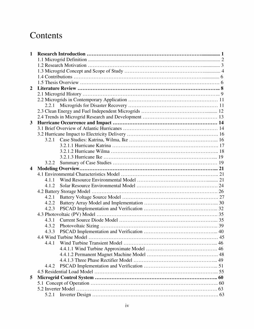
Figure 4.10: Response of Battery System from Discharging to Charging State

The system responds to the change in control input in a constant rate of change before settling to

the new operating point within 2 seconds. The oscillations dissipate a few seconds later. Finally

the efficiency of the battery system is given in Figure 4.11. The efficiency from terminal to

delivered power, of the battery array at a maximum power output of 10 kW is nominally 94.5%.

Note that high frequency oscillation in the efficiency shown in Figure 4.11 is due to inverter

circuit switching.

Figure 4.11: Battery System Efficiency at Nominal Discharge

Charging

Discharging

35

4.3 Photovoltaic (PV) Model

The photovoltaic model implemented in this microgrid system is referenced from [27]. It is a

classical PV model that uses a current source, series and shunt resistance, and a turn-on diode to

represent the behavior of a single cell. The model will be verified against the parameters of

commercially available BP Solar 200 Watt module.

4.3.1 Current Source Diode Model

Modeling of the PV array is performed by developing an equivalent circuit that represents the

characteristic performance of the current–voltage (I-V) curve for a given panel. The I-V curve

for the referenced panel is given in Figure 4.12.

Figure 4.12: The I-V curve for a BP 220 Watt module [28]

The most common PV model used in electric transient modeling is the single diode/current

source. In this model, the non-linear characteristics of the PV cell are captured in the diode turn-

on voltage. More advanced models have been proposed in [29] – [30], which have multiple

36

diodes in series and parallel to represent the I-V curve characteristic of a PV panel. However, for

this effort, the classical single diode equivalent circuit is implemented [27].

Figure 4.13: PV cell equivalent circuit model

To derive the values and/or dependencies for the equivalent circuit model, the following

relationships are derived as:

cellSHDsc IIII ++= , (4.13)

SHRshScellcell RIRIVS

⋅+⋅= . (4.14)

The current through the diode can be represented as

)1(0 −⋅=⋅

kT

Vq

D

D

eII , (4.15)

where

=0I Diode saturation current (A),

=q Magnitude of electron charge (1.6x10),

=k Boltzmann’s constant (1.38x10),

=DV Diode turn-on voltage (V),

=T Cell temperature (K).

37

From 4.14, it can be seen that Vd can be represented as the sum of the cell voltage plus the drop

across the series resistance. This results in the following expression

)1(

)(

0 −⋅=⋅+⋅

kT

RIVq

D

Scellcell

eII . (4.16)

Solving for cell current, the following relationship can be derived as [27]

SHDsccell IIII −−= , (4.17)

SH

ScellcellkT

RIVq

sccellR

RIVeIII

Scellcell ⋅+−−⋅−=

⋅+⋅

)1(

)(

0 . (4.18)

Knowing the characteristics of the cell, all the parameters can be calculated that are needed for

the model. The open-circuit cell voltage, not the general cell voltage, can be determined by using

the previous equation, and realizing that the cell generates no current in the open circuit

condition. Also, knowing that the shunt resistance is generally very large, it can be effectively

ignored for equivalent circuit calculations. Therefore, the open circuit voltage can be determined

as

)ln()1(00

,,

)0(

0

,

I

IVVeIII SC

celltcellOCkT

Vq

sccell

cellOC

⋅=→−⋅−==

+⋅

, (4.19)

where

q

TkV cellt

⋅=, (4.20)

Eq. 4.19 can now be used to solve the absolute diode current and eliminate that term from the

short-circuit current expression

cellt

cellOC

V

V

SC eII ,

,

0

−

⋅= , (4.21)

38

−=⋅⋅−=

⋅+−⋅+−

cellt

ScellcellOCcell

cellt

Scellcell

cellt

cellOC

V

RIVV

SC

V

RIV

V

V

SCSCcell eIeeIII ,

,

,,

, )()(

1 . (4.22)

Equation 4.22 is the final expression for the cell current. Since the Icell is also in the exponent,

an explicit solution is not possible. Therefore, for numerical solvers in MATLAB are used to

estimate the voltage & current pair. The next component to determine in the system is the series

resistance. By definition, the cell resistance is given by the ratio of fill-factors times the ratio of

open-circuit voltage to short-circuit current at standard test conditions (STC). This is expressed

as follows [27]

STCcellSCSTCcellOC

STCcellMPP

STCIV

PFF

@,@,

@,

⋅= , PV cell fill factor at STC, (4.23)

1

)72.ln(,0

+

+−=

STD

STDSTD

STCvoc

vocvocFF , Fill factor with normalized STC, (4.24)

where

cellt

STCcellOC

STDV

Vvoc

,

@,= , (4.25)

−=

STCcellOC

STCcellOC

STC

STC

cellSI

V

FF

FFR

@,

@,

,0

1 . (4.26)

The values for cell voltage, current, and maximum power can be determined directly from the

manufacturer’s datasheet for a given PV module. The final expressions needed for the model are

the correction factors for changes in solar irradiance and cell temperature. The relationship

between cell current and solar irradiance is directly proportional, whereas the relationship

between cell temperature and open circuit voltage are inversely proportional. The correction

factors, by definition, are given by

39

( )STC

STC

STCcellSCcellSC TTG

GII −+

= α@,, , (4.27)

( )STC

STC

celltSTCcellOCcellOC TTG

GVVV −+

⋅+= βln,@,, , (4.28)

where

=α Temperature coefficient of short-circuit current (A/° C),

=β Temperature coefficient of open-circuit voltage (A/° C),

=T Actual cell temperature (° C),

=STCT Rated STC cell temperature (° C), typically 25° C,

=G Actual solar irradiance (W/m²),

=STCG Rated STC solar irradiance (W/m²), typically 1000 W/m².

With the general PV model defined, the BP 200 specific parameters can be applied to the model

for implementation in PSCAD.

4.3.2 Photovoltaic Sizing

Using the constraints of available rooftop square footage, panel cost, and optimal array

orientation, the PV array can be sized appropriately. The electrical characteristics of the BP 3220

module are given in Table 4.1.

Table 4.1: Electrical Characteristics of the BP 3220 Panel [28]

Characteristic Value @ STC

Footprint 18 ft²

Maximum Power @ MPP 220 W

Voltage @ MPP 29.0 V

40

Current @ MPP 7.6 A

Short Circuit Current 8.4 A

Open Circuit Voltage 36.2 V

The PV array is scaled such that the PV array can supply the maximum daytime residential

demand with additional margin in the event of an atypical irradiation and also to supply excess

generation to the central battery array. Given these constraints, the PV array is sized for 3500 W

maximum output. This requires a minimum of 16, 220 W panels to satisfy this output. However,

the minimum of 16 panels is for normal operating parameters. The solar resource shown in

Figure 4.5 is below the rated output of the panels. The standard rule of thumb for derating of a

PV array for non-ideal solar resource is 125% DC to AC power ratio [31]. That is, 1.25 times the

rated AC power output is required from the DC power rating of the array. As a result, the total

number of panels required is 20 per array. The panels are tied in parallel to limit the magnitude

of the voltage swing seen by the inverter. Therefore, the DC link voltage will be within 5 Volts

+/- of the 29 V nominal MPP. With 20 panels in parallel, the maximum current through the DC

link will be almost 120 Amps. This is relatively high given the size of the unit. While it will

impact the overall efficiency of the inverter, it does allow for a relatively simple installation and

configuration of the array. The total square footage of the PV array is 288 ft², which is sufficient

for a standard home with ample space for spacing support structure for the panels.

4.3.3 PSCAD Implementation and Verification

The implementation of the PV array in PSCAD is realized through the control blocks and

electrical elements. The PV Array equivalent circuit is shown in Figure 4.14.

41

Figure 4.14: PV Array Equivalent Circuit Implemented in PSCAD

The calculation of the maximum power point in PSCAD is needed to determine the appropriate

setpoint for the inverter. The calculation is based on the approximation that the MPP voltage

occurs at approximately 73.3% of the open-circuit voltage [28]. Using this and filtering out the

switching harmonics with a FFT block, the MPP calculation carried out as shown in Figure 4.15.

It is important to note that MPP is tracked and calculated actively in modern inverter control

systems; however the 73.3% approximation is sufficient for the scope of this research. The open-

circuit voltage and short circuit voltage calculations are based on the equations given in 4.3.1.

The PSCAD implementation of the OC-Voltage and SC-Current are given in Figure 4.16.

Figure 4.15: Calculation of the Maximum Power Point Implemented in PSCAD.

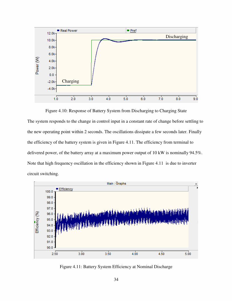
42

Figure 4.16: Short Circuit Current and Open Circuit Voltage Calculation in PSCAD.

The fill factor and resistance calculation are also implemented in PSCAD and are shown in

Figures 4.17-18. The parameters vary as the configuration of the array changes

Figure 4.17: Fill Factor Calculation for the PV Array.

43

Figure 4.18: Calculation of the Series and Shunt Resistance of the PV Array.

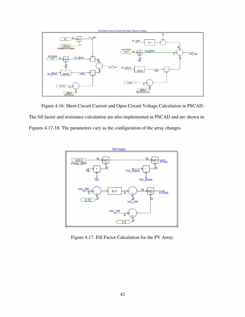
With the full system implemented in PSCAD, the performance of the model is verified. The

output of the PV array is dependent, primarily, on solar irradiance. As the solar irradiance varies,

the power output will vary accordingly. Figure 4.19 shows the change in output power as

irradiance varies. At time equals 5 seconds, the irradiance changes from a constant to a triangular

wave with a 10 sec period as the output varied from 1000 to 600 W/m². The system responds

accordingly with a slight lag due to the stored energy of the filtering. Finally, the efficiency of

the PV array is verified at full power. The nominal efficiency, from the terminals of the panel to

interconnection point, at maximum power is approximately 91.5%. Efficiency is higher at lower

power levels due to reduced line current. This is shown in Figure 4.20.

44

Figure 4.19: The Power Output Response to a Change in Solar Irradiance

Figure 4.20: Efficiency of the PV Array System which Includes Inverter Losses

45

4.4 Wind Turbine Model

The wind turbine generator (WTG) model for the microgrid systems is partially referenced from

[32] with several custom modeling features added. It is based on the permanent magnet machine

characteristics for generators attached to a varying source. While the design of the wind turbine

model is custom for this application, it does reference the Hummer Wind Power 5-kW unit to

apply practical limits to the WTG [33]. This unit is also referenced because it uses an auto-

adjusting yaw-drive axis, such that the turbine is always pointing in the direction of the wind. In

a low energy resource area, like Florida, this feature is important because it allows for maximum

energy harvesting in all wind directions, and also allows for a simpler model. Compared to the

battery and photovoltaic model where there is a single model entity, the wind turbine model

contains several discrete sub elements. The first is the wind turbine model which uses the input

of wind speed to drive the power level output. The second is the permanent magnet generator

which uses speed characteristics of the wind to vary the input torque to the generator and

produce a 3-phase sinusoidal output. The final segment is the 3-phase rectifier and filter which

rectifies to DC the output of the generator. Since these results in a significantly more complex

model than the solar and battery system, a block diagram is given in Figure 4.21.

Figure 4.21: Block Diagram of the Wind Turbine Transient Model

46

4.4.1 Wind Turbine Transient Model

The first step in developing the transient model is to determine the equations that drive the

transient model. The following sections cover the design of the individual sub-elements that

make up the turbine model.

4.4.1.1 Wind Turbine Approximate Model

Wind power uses the kinetic energy from the flow of air mass to generate electricity. The

relationship between the mass flow and the power produced is given by

25. vmE ⋅⋅= . (4.29)

This is the fundamental equation for kinetic energy. The energy of the mass of air through an

area is given as the following:

( ) 322 5.5.5. vAtpvAvtpvmE ⋅⋅=⋅⋅=⋅⋅= , (4.30)

where

=A The area the flow of wind passes through,

=p The density of air (approximately 1.2 kg/ 3m ),

=t total time energy is produced.

Solving for power gives the fundamental wind power equation, which is expressed as

35. vApt

EP ⋅⋅⋅== . (4.31)

The amount of energy extracted from the wind by the turbine depends on another important

factor, namely the tip-speed ratio (TSR). The TSR is defined as the ratio between the speed of

the turbine blade tip, time rotor radius, divided by the wind speed [34]. Finally we have

v

RTSR

Ω= , (4.32)

47

where

=Ω The rotational speed of the tip,

=R The rotor radius,

=v The wind speed.

From the previous equation it can be seen that this parameter varies as the wind speed varies. In

turbines with variable pitch, the tip speed ratio can be made relatively constant by adjusting the

blade geometry to maintain a constant speed on the tip. For fixed pitch application, which is used

in this implementation, the TSR will vary, while being at its maximum at rated power output of

the turbine. The last parameter that needs to be considered for the model is the coefficient of

power, Cp. The Cp is actually a ratio of extracted energy over total energy available. In a well-

designed turbine, the Cp ratio will be over 40% at its rated power output. It is also a function of

TSR. As the TSR varies, the Cp ratio will vary. The detailed relationship of these two quantities

is beyond the scope of this thesis, but using the fundamental relationship between the two, the

power Eq 4.31 can be further refined to take into account Cp as

( )TSRCpvApP ⋅⋅⋅⋅= 35. , (4.33)

where

Cp: Function of TSR.

For the implementation of the wind turbine in this model, it is important to realize that the full

machine dynamics of the turbine can be approximated for the electrical transient model. This is

important because it reduces the model complexity and decrease simulation runtime. Taking this

into account, the model of the turbine is therefore simplified into a lookup table. The lookup

table is based off the output of the Hummer Wind 5 kW turbine. Using the relationship between

power and wind speed shown in Fig. 4.22, the turbine model can be expressed as transfer

48

function of wind speed to mechanical power. Through a lookup table, this model can be directly

built into PSCAD (see section 4.4.2).

Figure 4.22: The Power Curve of the Hummer Power Unit [33]

4.4.1.2 Permanent Magnet Machine Model

The generator for the wind turbine is a permanent magnet (PM) generator. The latter is coupled

to the wind turbine, typically through a gearbox, to transfer energy from the turbine to the

generator. Its output varies as shaft torque and speed vary. This results in the generator

outputting a variable frequency and voltage magnitude. For this research, the existing machine

models in PSCAD are leveraged to develop the overall WTG model. The existing PSCAD

machine transient model is based on the park transformation of electric machines. The equations

that drive the model are given by

dt

d

dt

dirv r

d

q

qsq

θλ

λ++⋅= , (4.34)

dt

d

dt

dirv r

q

d

dsd

θλ

λ++⋅= , (4.35)

49

00

00 =+⋅=dt

dirv s

λ, (4.36)

dt

dir kd

kdkd

''0

λ+⋅= , (4.37)

dt

dir

kq

kqkq

''0

λ+⋅= , (4.38)

where:

kqmqqqq iLiL ⋅+⋅=λ , (4.39)

mkdmdddd iLiL 'λλ +⋅+⋅= , (4.40)

000 =⋅= iLlsλ , (4.41)

kqkqqmqkq iLiL ''' ⋅+⋅=λ , (4.42)

mkdkddmdkd iLiL '''' λλ +⋅+⋅= . (4.43)

Section 4.4.2 shows the PSCAD implementation of the PM machine model, consolidated into a

single block representation.

4.4.1.3 Three Phase Rectifier Model

From the permanent magnet generator, a rectifier is inserted into the circuit to rectify the output

to DC. There are several rectification types that can be implemented for this application. Active

rectification, where switching transistors are used instead of diodes to maintain a constant DC

voltage through variations in the front-end AC voltage, are widely used now in a number of wind

power electronics systems. However, given the relative small operating envelope that the PM

generator operates in and the need to a simple model for runtime optimization, a classical diode

rectification scheme is used. In the diode rectification model, the negative half-cycles are

inverted to the positive side and results in a crude DC output. As shown in Figure 4.23, the

50

rectifier outputs a rippled DC output that requires further filtering. The output voltage for a full

wave rectifier is the square-root of 3 times greater than the peak current as shown in

)cos(3)cos(33

ααπ

peak

peak

AVEDC VV

VV ⋅≈⋅

== , (4.44)

where

=DCV The fully rectified DC voltage,

=AVEV The average voltage of the rectified waveform,

=peakV The peak voltage of one AC line-line input waveform,

=α Firing angle for the rectifier (α = 0 for diode rectification).

Figure 4.23: The Effect of a 3-Phase Full Wave Rectifier

Finally, the filter capacitors for the rectifier can be determined from

fCR

VV

load

peak

ripple⋅⋅

= . (4.45)

For this application, the DC link serves no purpose other than to feed the inverter. As a result, the

inverter can accept a wide range of voltage inputs. It has the ability to boost low voltage input to

maintain the fixed output voltage on the interconnection side. As a result, a voltage swing of up

to +/- 5 Volts or a ripple voltage of 10 Volts is permissible. Like with the PV array, while a large

voltage swing can be managed by building it into the inverter controller design, limiting the

51

swing to less than 10 volts reduces simulation sampling time and simplifies the controller. Using

this constraint and referencing the Hummer Wind datasheet for nominal power output, the filter

capacitor can be calculated as

fVV

P

V

fVR

VC

ripple

RMS

nom

peak

rippleload

peak

⋅⋅

=

⋅⋅=

2

, (4.46)

( )

mFFC 072.3003072.

360102/48

5000

48

2

==

⋅⋅

= .

Note that the frequency of the full wave bridge is 6 times the fundamental frequency since all the

peaks are inverted to the positive waveform. The frequency is therefore 360 Hz. The capacitance

is rounded to the nearest decimal place. Therefore, 3 mF is an acceptable filter capacitor for the

rectifier.

4.4.2 PSCAD Implementation & Verification

The three independent sub-elements in Section 4.4.1 are consolidated into the full wind turbine

model that is implemented in PSCAD. The first segment is the wind turbine approximation

model shown in Fig. 4.24. This model inputs the wind speed and outputs the per unit rotational

speed of the turbine shaft based on a lookup table. The mechanical power generated is used to

determine the setpoint for the inverter controller. The PM machine model is an existing model

within PSCAD and one of the few consolidated models leveraged for this research as shown in

Fig. 4.25. The PM machine model inputs a rotational speed from the turbine and outputs a 3-

phase sinusoidal voltage. It also outputs the loaded electrical torque of the system for feedback to

52

the turbine, but it is not used in the application since the inverter load is set to match the turbine

rated power.

Figure 4.24: Wind Turbine Approximation Model

Figure 4.25: Existing PSCAD PM machine model.

Finally, the full wave diode bridge and filter capacitor, with equivalent ESR, are shown in Figure

4.26.

53

Figure 4.26: 3-Phase Rectifier Bridge for Wind Turbine Model

The model performance is verified by looking at the steady-state and transient response of the

turbine model to changes in wind speed. Electrical transient events are covered in Section 4.6.

The response of the real power output and reactive power load of the wind turbine is shown in

Figure 4.27. From that figure, it can be seen that the power output follows the change in wind,

but with a sharper slope since the power generated is the cube of the wind speed.

A

B

C

54

Figure 4.27: Wind Turbine Response to a Change in Wind Speed

Finally, the efficiency of the wind turbine is verified at nominal power. The nominal efficiency,

from mechanical shaft power to electrical point of interconnection, at maximum power is

approximately 79%. While the efficiency is relatively low, it is accurate of the specification of

the Hummerwind 5 kW unit. Higher efficiency can be achieved with large turbines, but this is

not part of the scope of this research. This is shown in Figure 4.28.

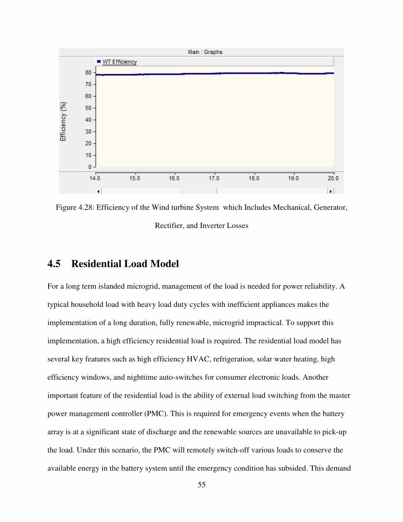
55

Figure 4.28: Efficiency of the Wind turbine System which Includes Mechanical, Generator,

Rectifier, and Inverter Losses

4.5 Residential Load Model

For a long term islanded microgrid, management of the load is needed for power reliability. A

typical household load with heavy load duty cycles with inefficient appliances makes the

implementation of a long duration, fully renewable, microgrid impractical. To support this

implementation, a high efficiency residential load is required. The residential load model has

several key features such as high efficiency HVAC, refrigeration, solar water heating, high

efficiency windows, and nighttime auto-switches for consumer electronic loads. Another

important feature of the residential load is the ability of external load switching from the master

power management controller (PMC). This is required for emergency events when the battery

array is at a significant state of discharge and the renewable sources are unavailable to pick-up

the load. Under this scenario, the PMC will remotely switch-off various loads to conserve the

available energy in the battery system until the emergency condition has subsided. This demand

56

management helps protect the microgrid from a complete system wide loss of power. To

determine the savings from a high efficiency home, the NREL-UCF report [35] on “smart

homes” in Florida is consulted. In this report, a control home and a high efficiency home are

referenced to determine the level of financial savings achieved from a high efficiency home with

rooftop solar PV panels installed. The comparison of the control home and the high efficiency

home are shown in Figure 4.29.

Figure 4.29: Hourly Energy Consumption Profile of a Standard Home and Home with PV and

High Efficiency Appliances [35]

According to the report, the high efficiency consumes 55% less energy throughout the day than

the standard home. This savings is applied across the yellow demand curve depicted in Figure

57

4.29. This results in the demand load profile in Figure 4.30. For a single home, the nameplate

generation from sections 4.3 and 4.4 give 8.6 kW of generation and 2.3 kW peak demand from

the residence. The surplus of generation is made up for by the inconsistent wind resource in

Florida, the need to store energy in the central battery array, and 50% margin for loss of up to 2

renewable sources in the microgrid. As a result, for a single residence, the average hourly wind,

solar, and demand are plotted together in Figure 4.31. The total energy generated versus energy

consumed is shown in Figure 4.32.

0 5 10 15 200

500

1000

1500

2000

2500

3000

Time of Day (hr)

Pow

er

(W)

Customer Demad

Figure 4.30: Hourly Demand Curve for High Efficiency Microgrid Home

58

0 5 10 15 200

500

1000

1500

2000

2500

3000

3500

4000

Time of Day (hr)

Pow

er

(W)

Customer Demad

Solar Power Generated

Wind Power Generated

Figure 4.31: Single Residence Average Hourly Generation and Demand Profile

59

0 5 10 15 200

10

20

30

40

50

60

Time of Day (hr)

Energ

y P

roduced/C

onsum

ed (

kW

h)

Generation (Wind + Solar)

Demand

Figure 4.32: Total Average Energy Generated and Consumed in a Single Residence

In Figure 4.32, it can be seen that during the early nighttime hours, generation is less than

demand and energy must be pulled from the central battery array. After approximately 10 am the

generation and load become equal and afterwards generation becomes greater in demand. The

excess energy is either stored in the battery array, or one or more generation units will be turned

off to meet demand. This forms the basis of the residential demand model. Note that this is the

typical case, and margin is provided to correct for sustained periods of abnormal operation.

60

Chapter 5

Microgrid Control System

This chapter provides an overview of the layered control system for the microgrid. The controller

utilizes top level control through the power management controller (PMC) that regulates system-

wide power flow and local control through PQ power regulation with droop control. The PMC

implemented balances supply and load with available resource and battery capacity. The PMC

presented in this thesis is an introductory step in the design of this style of microgrid control.

Droop control for island mode operation is also covered in this section.

5.1 Concept of Operation

The microgrid is designed to operate in two principle modes of operation: grid-connected and

island mode. Since this particular application is for disaster recovery, the emphasis is on

sustainable island mode operation. The control system is tiered such that local droop control are

contained with the generating units and higher level dispatching is centralized. Figure 5.1 shows

the control pyramid for the microgrid.

61

Figure 5.1: Top-Level Controller Hierarchy

For both modes of operation, the inverters for the renewable sources set their power flow based

off a reference voltage and phase angle. In the case of grid-connected mode, this is the

distribution voltage at the common bus. In the case of islanded mode, the reference is the output

of the battery inverter module. Because of this, it is the principle operation of the battery to

emulate the behavior of the distribution network during island mode. Therefore the battery

system shall maintain a relatively constant voltage as the units are brought online and be able to

deliver power or absorb power depending on the level of power being generated. These two

modes of operation are illustrated in Figure 5.2.

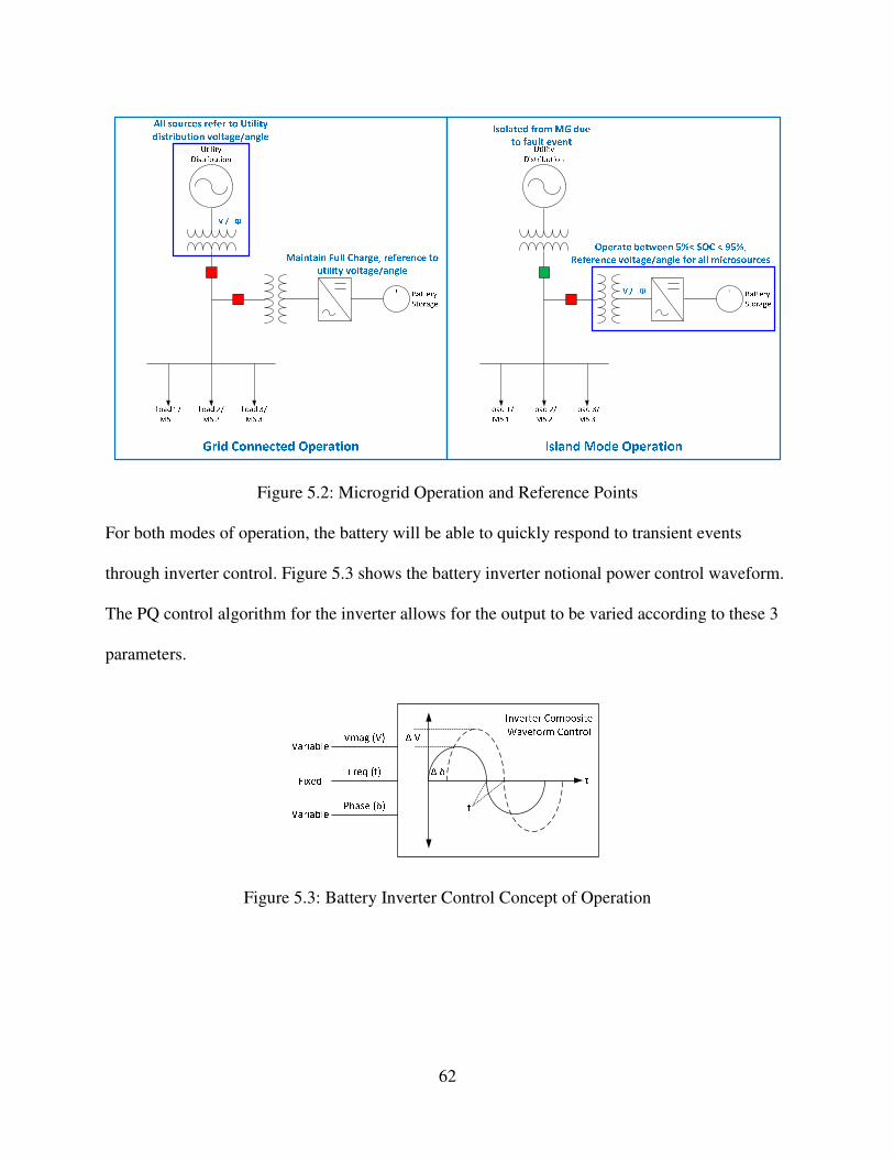
62

Figure 5.2: Microgrid Operation and Reference Points

For both modes of operation, the battery will be able to quickly respond to transient events

through inverter control. Figure 5.3 shows the battery inverter notional power control waveform.

The PQ control algorithm for the inverter allows for the output to be varied according to these 3

parameters.

Figure 5.3: Battery Inverter Control Concept of Operation

63

5.2 Inverter Model

The fundamental hardware element of the microgrid control is the inverter. The latter handles

real power and reactive power flow to and from the sources connected to it. The inverter model

implemented for this research is the H-Bridge single-phase inverter. This inverter design is

advantageous over other single-phase inverter designs, primarily because it allows for variable

sinusoidal voltage output with only half of the peak-peak voltage applied on the DC link. This

results in switching at much lower voltages. Figure 5.4 is referenced from [36] and shows a

typical configuration for an H-Bridge inverter from DC source to grid connection. The inverter

model and controller design for this research provides for a low level of fidelity and design

details. In chapter 8, recommendations are made to improve the controller design and include

bandwidth limitation, hardware constraints, and higher order filter design. However, the

proposed inverter model for this research is sufficient for analytical studies.

Figure 5.4: H-Bridge Inverter with Filtering and Grid Connection

5.2.1 Inverter Design

The inverter hardware design consists of the power electronics bridge, filter, and isolation

transformer. The bridge consists of 4 transistors, with fly-back diodes, switching at 10 kHz. This

Vmg Vg Vg

64

switching frequency was selected to reduce the size of the filtering. While ideally the switching

frequency should be set as high as possible to reduce filtering, it must be traded with physical

limitations of the circuit and latency of the switching controller. For the simulation, the switching

time should be limited such that the simulation runtime does not become excessively long. The

nominal output voltage for the bridge is 48 volts nominal for the renewable sources. This voltage

is selected to match the nominal voltage of the renewable sources and limits the size of the

flyback diodes for switching transients. For the battery array, 125-V nominal is selected due to

its requirement of being able to charge and discharge into the entire microgrid. The only changes

between the hardware of the 48-V and the 125-V bridge are the filtering devices and the isolation

transformer sizing.

The inverter bridge is designed to be universal between the 3 sources (i.e. PV array, WT, and

battery array). Therefore, its maximum power rating will be based on the maximum power flow

through the battery array. The maximum load of the battery system is 7.5 kVA nominal.

Allowing for 33% additional margin for short term transients, the maximum size of the inverter

is 10 kVA. For the 48-V bridge design, this results in a maximum current flow of 208 A and 80

A for the 125 V bridge.

The switching devices used for this inverter are insulated gate-bipolar transistor (IGBT). The

IGBT is a versatile power electronics device that is well suited for power switching applications.

In Figure 5.5, it can be seen that IGBT meets the requirements for the inverter bridge defined in

this section (i.e. 48V/125V, 10 kVA, and 10 kHz switching).

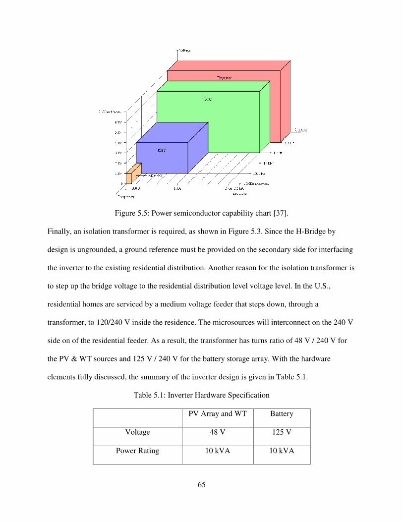
65

Figure 5.5: Power semiconductor capability chart [37].

Finally, an isolation transformer is required, as shown in Figure 5.3. Since the H-Bridge by

design is ungrounded, a ground reference must be provided on the secondary side for interfacing

the inverter to the existing residential distribution. Another reason for the isolation transformer is

to step up the bridge voltage to the residential distribution level voltage level. In the U.S.,

residential homes are serviced by a medium voltage feeder that steps down, through a

transformer, to 120/240 V inside the residence. The microsources will interconnect on the 240 V

side on of the residential feeder. As a result, the transformer has turns ratio of 48 V / 240 V for

the PV & WT sources and 125 V / 240 V for the battery storage array. With the hardware

elements fully discussed, the summary of the inverter design is given in Table 5.1.

Table 5.1: Inverter Hardware Specification

PV Array and WT Battery

Voltage 48 V 125 V

Power Rating 10 kVA 10 kVA

66

Current 208 A 80 A

Switching Frequency 10 kHz 10 kHz

Power Semiconductor IGBT IGBT

Isolation Transformer 48 V / 240 V 125 V / 240V

The last element of the hardware design, which also feeds the controller design, is the LC filter.

It is discussed next.

5.2.2 LC Filter Design

A well designed filter is important for reducing harmonics generated by the bridge. It allows

margin for reactive power control, and maintains stability through transient events. For this

application, a traditional LC filter is selected. The LC filter provides blocking of high-order

harmonics through a low-pass filter. The filter is tuned such that the 10-kHz switching and all

associated odd number harmonics are filtered out while maintaining the fundamental sinusoid.

The resonance frequency of the filter is given by

LC

f resπ2

1= . (5.1)

The resonance frequency ideally defines the spot where the frequency components below

frequencies are passed through and components above are blocked. In a real filter, the resonance

frequency represents the point where blocking begins and signal attenuation continues until the

higher frequency harmonics are at a negligible power level. The gain of the filter is important as

well for understanding the impact of the filter on system output. As shown in [38] the filter gain

is expressed as

67

( )( )( ) 2

00

1

2

1

1

++

==

ωω

s

Q

ssv

svsG , (5.2)

where

00 2 fπω = the resonance frequency of the filter,

L

CRQ = the quality factor of the filter.

The Q factor is used as part fo the design criteria. A Q factor larger than 0.5 results in an

underdamped system where a change in input will result in a sinusoidal and exponential decay to

the new setlling value. However, for very large values of Q, the greater the amplitude and the

longer the settling time. As a result, the filter is designed such that the Q value is optimized. For

determining the value of L and C, the following constraint for a well designed LC filter for AC

inverters is applied [39]:

210 0

swres

ωωω ≤≤ , (5.3)

2

0 ratedV

PC

⋅

⋅=

ω

α, (5.4)

where

=0ω Rated AC frequency of inverter (377 rad/sec),

=swω Switching frequency of the inverter bridge (62,381 rad/sec),

=α Reactive power factor (<5% for WT & PV array, 15% nominal for battery).

The filter capacitance for the battery array was determined for the battery array and WT & PV

inverter filters was determined and shown in Table 5.2. The value of the inductance is found

using the equation given in Eq 5.1. Through iteration to find the appropriate resonant frequency,

68

that satisfies the constraint in Eq 5.3, the values for inductance are given in Table 5.2. The full

design of the filter design is given below. The value of Q is sufficient for both applications and

the filter resonant frequency satisfies all constraints.

Table 5.2: LC Filter Specification

Battery Array WT & PV Array

resω 750 rad/sec 2,250 rad/sec

L 150 µH 50 µH

C 300 µF 100 µF

V 125 V 48 V

P 10 kW 5 kW

Q factor 2.21 0.65

5.2.3 Inverter PQ Controller

The controller for the inverter is based on the PQ control theory for power flow-calculation [36].

It provides the fundamental relationship between real power and phase angle, as well reactive

power and voltage differential. The relationship for power flow through an arbitrary point on an

electrical network can be stated as

( )δsinX

VVP

gmg ⋅= , (5.5)

( )

X

VVVQ

gmgmg δcos2

⋅⋅−= , (5.6)

where

=mgV The AC voltage of the microgrid source,

69

=gV The AC voltage of the point of interconnection,

=δ The phase angle difference between the two voltages,

=X The impedance of the equivalent inductance between the two voltages (usually a

transformer).

From Eqs. 5.5-5.6, the values of Vg and X are fixed by the network and are not practically

adjustable. However, the values of Vmg and δ are directly controllable by adjusting the PWM

sequence feeding into the IGBT bridge. The relationship between varying these two parameters

can be seen by taking the partial derivatives of the previous equations. For varying Vmg and δ,

the effect on real and reactive power are determined by deriving their partial derivatives with

respect to these variables, yielding

( )δsinX

V

V

P g

mg

=∂

∂, (5.7)

( )δδ

cosX

VVP gmg ⋅=

∂

∂. (5.8)

It can be seen from Eq 5.7 that varying the voltage has no impact on the power output, for small

deviations, due to the term being eliminated by the partial derivative. However in Eq. 5.8, it can

be seen that varying the phase angle has an impact on the changing power output. Similarly, we

derive the partial derivative of the reactive power with respect to Vmg and δ to get

( )

X

VV

V

Q gmg

mg

δcos2 ⋅−⋅=

∂

∂, (5.9)

( )X

VVQ gmg δ

δ

sin⋅⋅=

∂

∂ . (5.10)

It initially appears that both the phase angle and voltage have an impact on the reactive power,

but constraints still need to be applied. It is important to note that the value of the angle δ is

70

generally quite small (typically smaller than < 10°). Therefore, the sinusoidal function in Eq.

5.10 is typically very small for changing Q. As a result, the reactive power changes little for

changing voltage angle. By the same constraint the cosine function is very close to 1, and

therefore the right-side of Eq. 5.9 is a constant, and the Q value is directly proportional to the

change in Vmg. In summary, the control relationship between real power P is related to varying δ

and reactive power Q is related to varying Vmg. This is shown in Figures 5.6-5.7. The feedback

loop is based on transfer function relationship in implicitly stated in Eq. 5.8 and 5.9, respectively.

The PI controller is tuned experimentally in MATLAB to find the maximum points for stability.

Given the difference in voltage magnitude and filter size, the gains are slightly different for the

battery array as they are for the PV array and WT model.

Figure 5.6: General Control Loop for Real Power Control

Figure 5.7: General Control Loop for Reactive Power Control

71

Finally, the parameters for Vmg and δ need to be converted into a PWM train. This is performed

by using a carrier wave to sample and digitize the composite sinusoidal output of the controller.

A comparator is implemented to perform this task and mark the output high or low depending on

which signal is higher at a discrete point in time, the composite sinusoid or the carrier wave. This

output is shown in Figure 5.8. Finally, the truth table for the IGBTs is given in Table 5.3. It

shows the operating states of the inverter and its associated output.

Figure 5.8: PWM Train Generated from Carrier Signal [40]

Table 5.3: Truth Table for the H-Bridge Inverter

Q1 Q2 Q3 Q4 Output

1 0 0 1 Positive Half Cycle

1 0 1 0 Zero Output

0 1 1 0 Negative Half Cycle

0 1 0 1 Zero Output

72

5.2.4 PSCAD Implementation

With the inverter controller design complete, the full system can be modeled in PSCAD. In the

latter, the inverter hardware and control models are implemented using existing electrical and

control blocks. The comparator control circuit is shown in Figure 5.9. It is implemented as a

controlled sine wave generation with variable angle and magnitude input. The carrier signal

generator operates at a fixed 10 kHz. The full PSCAD implementation of the inverter bridge

electrical circuit is shown in Figure 5.10. The system in PSCAD also includes fly-back diodes to

prevent shorting of the DC input.

Figure 5.9: PWM Generator for PQ Controller

Figure 5.10: H-Bridge, LC Filter, and Isolation Transformer for the Inverter Circuit

73

The PI controllers for the PQ feedback loops are shown in Figure 5.11-5.12. The PSCAD

implementation for the P control includes an additional step for limiting the power setpoint to a

realistic value for the source, as well as a conversion of units from MW to W for power.

Verification of the output of the inverter is shown in Figure 5.13. Two-phase shifted sinusoids

can be seen.

Figure 5.11: Control Loop for Real Power/Angle Control

Figure 5.12: Control Loop for Reactive Power/Voltage Control

74

Figure 5.13: Verification of Voltage Output from the Inverter against Grid Voltage

Finally the voltage and current THD for the inverter in steady state operation are shown in Figure

5.14-5.15. From IEEE 1547, the THD is required to be less than <5% for TDD which is satisfied

by both current and voltage quantities.

Figure 5.14: Currrent Harmonic Spectrum for Inverter at Full Load

75

Figure 5.15: Voltage Harmonic Spectrum for Inverter at Full Load

5.3 Power Management Controller

During the grid-connected mode of operation, any excess generation or significant droop events

will be handled by the distribution power system that the microgrid is connected to. For island

mode operation, this is not the case and a local supervisory power control is required. For this

reason, the power management controller (PMC) is developed. The PMC serves 2 functions. The

first is balancing supply and load over the long term through curtailing generation units for

excessive generation. The second is to curtail demand during an emergency event with low

renewable production and low battery SOC. The top level control diagram for the PMC is shown

in Figure 5.16. The input parameters are on the left-hand side and the output control is on the

right. During island mode operation, short-term transients are handled by regulating the battery

array and not the PMC. The PMC is designed to provide long time scale stability to the system

by balancing source, generation, and battery SOC. The full breadths of capabilities for the PMC

load balancing controller are shown in Table 5.4.

76

Figure 5.16: PMC Top-Level Control Diagram

Table 5.4: PMC Load Balancing Truth Table

Source Demand Battery SOC PMC Action

High High High

(SOC > 95%)

No Action if Psource ≈ Pdemand, Else switch off

generation and discharge battery

High High Low

(.5 < SOC < .95)

Charge battery

High Low High Switch off source until Psource < Pdemand,

Discharge battery

High Low Low Charge battery

77

Low High High Discharge battery

Low High Low Discharge battery, once SOC < 50%, start

load curtailment

Low Low High Discharge battery, once SOC < 50%, start

load curtailment

Low Low Low Discharge battery, once SOC < 50%, start

load curtailment

5.3.1 Island Mode Power Flow Balancing

During island mode operation, long-term dispatch of generations is critical and is limited by the

SOC of the battery array. Short of transient events, this control function is needed to compensate

for changes in environmental resources, battery charge state, and current demand. The system

action is based on three inputs, namely resource availability, power demand, and battery SOC.

The implementation of the truth table shown in Table 5.4 is accomplished by using a sequential

switching algorithm. If generation is too high and the battery is fully charged, WT1 will be

switched off first. After a short-time delay, the power measurement will be performed again. If

generation is still too high, WT2 will be shut off. This will continue for WT3 before switching

off of the PV arrays begins. The wind turbines are switched off first because they are most likely

to running at some point throughout the day, whereas the PV modules have a fixed prescribed

period for generation (i.e. daylight hours). This cascading switching off of units will continue

until generation drop below demand and the battery begins to discharge. Once the battery SOC

drops below 95%, units will begin to be switched online in reverse order. This transition is

captured in Figure 5.17.

78

Figure 5.17: Power Balancing Function Implementation in PSCAD

5.3.2 Environmental Resource Monitor

The environmental resource monitor shuts off generation sources when the environmental

parameters go out of their boundary for delivering useful power. For PV array, it is when the

irradiance is too low to provide enough regulation voltage to drive the inverter. By definition,

this limit is for direct irradiance, less than 100 W/m². For the WTG, it is when the wind speed is

either too low to generate the minimum voltage necessary for the inverter or the wind speed is

too high or pushes the mechanical limits of the WTG assembly. By definition, this limit is wind

speed above 20 m/s and speeds below 3 m/s. The only action for the PMC to take is to

disconnect the unit or reconnect depending on the state of the environmental condition.

For implementation in PSCAD, the monitors are modeled as comparators with a reference value.

The reference value is the minimum thresholds that the PV and WTG can operate at. An output

value of HIGH or 1 refers to the breaker operation to disconnect all of the sources impacted by

the low resource condition. This implementation can be seen in Figure 5.18.

79

Figure 5.18: Wind/Solar Resource Monitor Implementation in PSCAD

5.3.3 Emergency Load Control

For situations where the battery SOC is low and there are little to no generation available by the

renewable sources, curtailment of demand is required. This capability is added to the PMC

despite the fact that for most normal operational scenarios, curtailment does not occur. Power

curtailment in this microgrid is directly proportional to the SOC of the battery array. When the

battery array is low, power demand will be clamped low. The opposite situation occurs in high

SOC conditions. For the purpose of this thesis study, the mechanism of curtailment is not

expanded beyond a fixed load value. In practical applications, curtailment would occur by

remotely disconnecting large loads from the residences. Typically, remotely operated relays

switch off loads such as HVAC units, refrigeration, or electric hot water heater systems during a

period of weak supply. Expanding the complexity of the load model is beyond the scope of this

research effort. In this model, the load is discretely reduced as the battery SOC passes certain

setpoints. The load will be curtailed as the SOC drops below 50%, 25%, 10%, and 5% with the

80

last value being where the load is completely shut off. Implementation in PSCAD involves a

measurement of the current battery SOC and comparators. As the SOC drops below the threshold

value, the comparator will activate a HIGH or value 1 to command the assigned breaker to open.

This can be seen in Figure 5.19.

Figure 5.19: PMC Emergency Load Control Implementation in PSCAD

5.4 Island-Mode Droop Control

Maintaining stable power flow dynamics in the microgrid during islanding mode is handled by

droop control. The droop controller is lower level control of the PMC that manages short

duration transients in the microgrid. The droop controller will respond to transient changes on

the network and compensate accordingly. The inverter for the central battery module will

perform all droop control activities. The classical curves for P vs. ω and Q vs. V droop are

shown in Figure 5.20.

81

Figure 5.20: Droop Characteristics for Frequency and Voltage

One constraint to this classical implementation is the relatively short distances between

generation units and the low inertia of the network, which can result in instability during

frequency droop control. This can be mitigated using phase-angle droop control over frequency

control. Given that generation for this microgrid is entirely inverter-based and that inverters can

change their phase angle output instantaneously, phase-droop control can be implemented.

Phase-droop control has been proposed in [41] as ways of providing greater stability in weak

networks that have little system inertia. Given that the implemented microgrid has no direct

rotating mass for generation, phase control can offer the benefit of greater stability. In this

implementation, the frequency is fixed at 60 Hz, with a feedback loop to prevent long term error

in frequency output. The voltage and phase-droop control are handled primarily by the battery

array. As changes in supply and load occur throughout the microgrid, the battery array

compensates to maintain normal operation. Consequently, the two different modes of operation,

require two different control loops. For grid-connected mode, the control loop is set to an

arbitrary value for P and Q to output V and δ. For island mode operation, P and Q output are not

specified, while the voltage and phase angle magnitudes are maintaned constant. For island

mode, the control loop is a direct feedback for voltage and phase angle. As a result gain, values

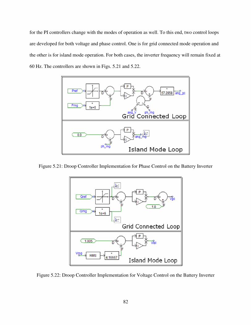
82

for the PI controllers change with the modes of operation as well. To this end, two control loops

are developed for both voltage and phase control. One is for grid connected mode operation and

the other is for island mode operation. For both cases, the inverter frequency will remain fixed at

60 Hz. The controllers are shown in Figs. 5.21 and 5.22.

Figure 5.21: Droop Controller Implementation for Phase Control on the Battery Inverter

Figure 5.22: Droop Controller Implementation for Voltage Control on the Battery Inverter

83

The voltage and phase response during island mode are shown in Figures 5.23 and 5.24. The

response droop for the voltage is less than 10% overshoot and well within the operational limits.

The droop control for the angle drops over 20% before recovery, but stabilizes in a relatively

short period. Stability is maintained during the transient events. With the droop control modeled,

the full model can be integrated.

Figure 5.23: Voltage Transient Response with Droop Control

Figure 5.24: Phase Transient Response with Droop Control

84

Chapter 6

Integrated Microgrid Model and Steady-State

Verification Results

This chapter reviews the integration of the hardware models developed in Chapter 4, along with

the control models in Chapter 5, into a complete microgrid top-level model. This complete model

will provide the ability to run numerous transient scenarios with respect to the microgrid

performance and response. While the microgrid presented here is limited to 3 residences, it is

scalable to a much larger number of residences. The constraint of 3 residences is to limit

simulation runtime while still showing the performance of the microgrid.

6.1 Microgrid Implementation in PSCAD

The full implementation in PSCAD requires that the submodels developed in Chapter 4 are

consolidated into a single top-level model. The consolidation requires simplification of

distribution transformers and breakers to improve simulation time and reduce model complexity.

The consolidations of the transformers are discussed in 6.1.1 and the full PSCAD model

presented in 6.1.2.

6.1.1 Transformer and Line-Loss Consolidation

To improve simulation runtime and reduce the complexity of non-vital system elements, the

transformers shown in Figure 1.3 are reduced to their equivalent impedances. This is further

simplified by neglecting the transformer resistive losses as well as core losses and focuses on the

85

inductive impedance of the series connection. By doing this, system-wide voltage will be

referenced to the residential 240 V. It is assumed that a 7% impedance transformer is used. This

results in approximately 200 µH equivalent inductance. It is also assumed that the distribution

line segments are no longer than 100 yards for any distance between residences and the central

battery array bus tie-in point. For simplicity, all line segments are assumed to be 100 yards in

length. The underground distribution cables are assumed to be 1/0 AWG conductor size and

approximated to be 30 mΩ for each 100 yard segment [42].

6.1.2 PSCAD Microgrid Model

The full model is consolidated into Figure 6.1. The test configuration is of a notional microgrid

network. It is an example of a common, but certainly not the only, single- phase distribution

scheme.

Figure 6.1: Microgrid Implemented in PSCAD

86

6.2 Microgrid Steady-State Performance

Prior to the transient analysis performed in Chapter 7, the model is first verified that it can

operate in steady-state mode. Steady-state operation is examined for two states, namely grid-

connected and island-mode operation. The scenarios described next will serve to verify the

steady state stability of the model.

6.2.1 Grid-Connected Steady-State Operation

The first scenario to be validated is that the system reaches a steady-state value for power,

voltage, and frequency in grid-connected mode. Here, the grid connection will be maintained and

all sources will be at their full power output. Table 6.1 provides the complete generation

configuration for this scenario. During this scenario, all of the breakers in Figure 6.1 are closed

(red). The simulation results are shown in Figure 6.2-6.4. From the results it can be seen that

power, voltage, and frequency results are constant for all sources.

Table 6.1: Grid-Connected Mode Steady State Operation Unit Status

Grid Battery PV Arrays WT Generators Load

Unit Status Online

Discharging

(10 kW)

3 kW

(1000 W/m)

4 kW

(10 m/s)

6 kW

1 kVAR

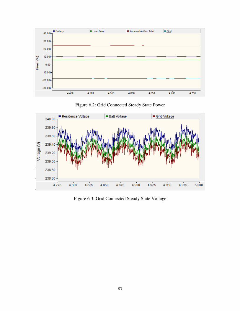
87

Figure 6.2: Grid Connected Steady State Power

Figure 6.3: Grid Connected Steady State Voltage

88

Figure 6.4: Grid Connected Steady State Frequency

6.2.2 Island-Mode Steady-State Operation

The second scenario to be validated is that the system reaches a steady-state value for power,

voltage, and frequency in island-mode operation. For this first scenario, the grid connection will

be disconnected and all sources will be at their full power output. The transition from a grid

connected mode will not be presented here as it is covered in Chapter 7. Table 6.2 provides the

complete generation configuration for this scenario. During this scenario, all of the breakers in

Figure 6.1 are closed (red), except for the BRK_grid which is open (green). The simulation

results of this scenario are shown in Figure 6.5-6.7. From the results it can be seen that Power,

Voltage, and Frequency results are constant for all sources.

Table 6.2: Island Mode Steady State Operation Unit Status


Unit Status Offline

Charging

(-17.5 kW)

3.5 kW

(1000 W/m)

4 kW

(10 m/s)

6 kW

1 kVAR

89

Figure 6.5: Island Mode Steady State Power

Figure 6.6: Island Mode Steady State Voltage

90

Figure 6.7: Island Mode Steady State Frequency

91

Chapter 7

Transient-Simulation Scenarios and Results

With the microgrid now completely developed, transient analysis can be performed for multiple-

operational scenarios. The simulation results presented here cover short-term and long-term

transient responses to very common electrical network events. A total of 8 transient events are

presented.

The measurement points for the simulations are shown in Figure 7.1. Note that the residence

voltages are only measured at one point. Based on earlier assumptions, it is assumed that each

generation and load will behave the same in parallel for each residence, implying that multiple

measurements are not necessary. The medium voltage measurements will be referred to the

secondary side of the load transformers and will be measured at 240 V nominal.

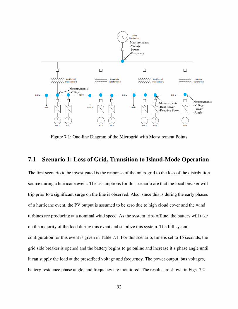
92

Figure 7.1: One-line Diagram of the Microgrid with Measurement Points

7.1 Scenario 1: Loss of Grid, Transition to Island-Mode Operation

The first scenario to be investigated is the response of the microgrid to the loss of the distribution

source during a hurricane event. The assumptions for this scenario are that the local breaker will

trip prior to a significant surge on the line is observed. Also, since this is during the early phases

of a hurricane event, the PV output is assumed to be zero due to high cloud cover and the wind

turbines are producing at a nominal wind speed. As the system trips offline, the battery will take

on the majority of the load during this event and stabilize this system. The full system

configuration for this event is given in Table 7.1. For this scenario, time is set to 15 seconds, the

grid side breaker is opened and the battery begins to go online and increase it’s phase angle until

it can supply the load at the prescribed voltage and frequency. The power output, bus voltages,

battery-residence phase angle, and frequency are monitored. The results are shown in Figs. 7.2-

Measurements:

-Voltage

-Power

-Frequency

Measurements:

-Voltage

-Power

-Angle

Measurements:

-Real Power

-Reactive Power

Measurements:

-Voltage

93

7.5. From the previous figures, it can be seen that the microgrid stabilizes in a short period of

time. The power transient lasts for less than 150 ms for the load. As the battery is brought online,

the system voltage rises rapidly to bring the battery to a full discharge state, but settled back to a

nominal 240 Volts once the battery and the 3 WTG’s balanced the load properly. In this scenario,

the output from the WTG’s drooped significantly as the changeover from grid to battery

reference angle occurred, however, once the battery had reach peak output, the WTG’s began to

supply more power to the load. It also important to note that the system frequency overshot was

significant during the switchover. However since all of the sources are asynchronously

connected, the system stabilized quickly due to phase angle droop control.

Table 7.1: System Configuration for Scenario 1


Before Event Online

Trickle

Discharge

Offline

Online

4 kW Power

(6 m/s Wind)

9 kW

3 kVAR

After Event Offline Discharge

No

Change

No Change No Change

94

Figure 7.2: Power Load Demand and Supply from PV, Batt, and WTG

Figure 7.3: System Voltages for the Common Bus, Residence Bus, and Battery Bus

Grid Connected Mode

Island Mode Transition

Island Mode

Steady State

Island Mode Transition Grid Connected Mode Island Mode

Steady State

Switching

Occurs

95

Figure 7.4: Battery Phase Angle Change (w.r.t. to Residence Bus)

Figure 7.5: System Frequency Response during Transition

7.2 Scenario 2: Island Mode - Interconnecting PV Microsources

The second scenario to be investigated is the switching on the PV array during island mode

operation. The assumptions are that battery array is 100% supporting all of the load centers. This

is a very likely scenario for after a hurricane once the wind speed is reduced and the sun has

come back out. Therefore, the WTG does not produce any power in this case. Here, the PV array

High Frequency Response

Grid Connected Mode

Island Mode Transition

96

needs to be switched online to relieve the battery array of supplying the entire load. The full

system configuration for this event is given in Table 7.2.



Before

Event

Offline Discharging Offline Offline

6 kW

3 kVAR

After

Event

Offline Charging

Online

(1000 W/m²)

Offline

No

Change

During the simulation, when the elapsed time equals 10 seconds, the PV arrays will switch

online and battery goes from a discharging mode of operation to a charging mode. It is assumed

that the battery has been operating for a long time and load curtailment is activated until the

battery has fully recharged. The results of the simulation are given in Figs. 7.6-7.10. It can be

seen from the simulation results that the introduction of the PV array to the microgrid allowed

for a very gracefully transition from battery discharge to charging mode with the load power

being maintained. The frequency drooped significantly as a result of the transition, but the low

value mark is still within the range of most modern electronic hardware tolerances [43].

97

Figure 7.6: Change in Power Output during Transition

Figure 7.7: Change in PV and Battery Output during Transition

Switching

Occurs

Battery

Discharging

Battery Charging

PV Ramp Up

Load Remains Constant

Battery Charging

PV Ramp Up

Load Remains Constant

Switching

Occurs

Battery

Discharging

WTG Remains Offline

98

Figure 7.8: Voltage Response during Transition

Figure 7.9: Frequency Response during Transition

Switching

Occurs

10%

Overshoot

Voltage Settles

<150 ms

Switching

Occurs

Frequency Settles

in <150ms

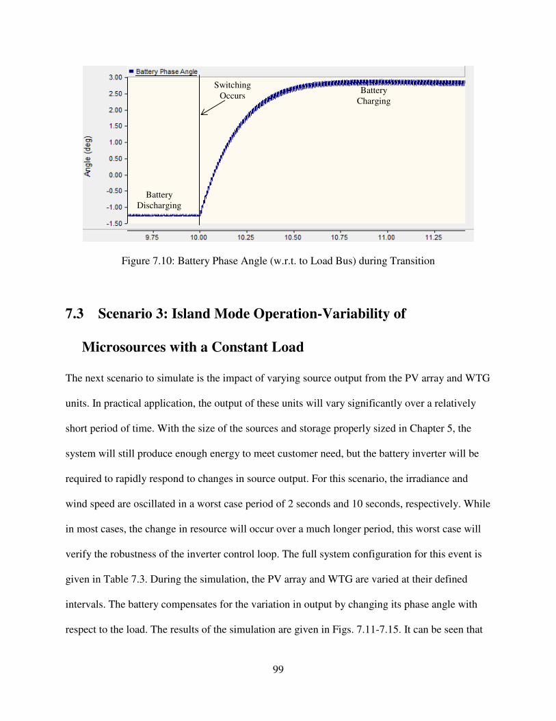
99

Figure 7.10: Battery Phase Angle (w.r.t. to Load Bus) during Transition

7.3 Scenario 3: Island Mode Operation-Variability of

Microsources with a Constant Load

The next scenario to simulate is the impact of varying source output from the PV array and WTG

units. In practical application, the output of these units will vary significantly over a relatively

short period of time. With the size of the sources and storage properly sized in Chapter 5, the

system will still produce enough energy to meet customer need, but the battery inverter will be

required to rapidly respond to changes in source output. For this scenario, the irradiance and

wind speed are oscillated in a worst case period of 2 seconds and 10 seconds, respectively. While

in most cases, the change in resource will occur over a much longer period, this worst case will

verify the robustness of the inverter control loop. The full system configuration for this event is

given in Table 7.3. During the simulation, the PV array and WTG are varied at their defined

intervals. The battery compensates for the variation in output by changing its phase angle with

respect to the load. The results of the simulation are given in Figs. 7.11-7.15. It can be seen that

Battery

Discharging

Battery

Charging

Switching

Occurs

100

the system remains stable while the sources fluctuate. The battery inverter is able to keep power

supply to the load effectively constant as the sources are varying. Since only real power was

being varied, only marginal changes in voltage output were observed.



Unit

Status

Offline

Discharging/

Compensation

5 ↔ 9 kW

(600-1000 W/m²)

.3 ↔ 4 kW

(4-6 m/s)

16 kW

4 kVAR

Figure 7.11: Worst Case Solar Irradiance Variation Frequency

Figure 7.12: Worst Case Wind Speed Variation Frequency

101

Figure 7.13: Power Output Resulting From Resource Variation

Figure 7.14: Voltage Response to Changing Renewable Sources Variation

Voltage Variation within

Normal Bounds

Battery Response to

Source Variation PV Linear

Response

WTG Cubic

Response

Voltage Variation within

Normal Bounds

102

Figure 7.15: Battery Phase Angle Response to Changing Renewable Sources Output

7.4 Scenario 4: Island Mode-Wind Gust Ride Through

Another environmental scenario to analyze is the impact of wind gusts on the system

performance. Unlike PV arrays, which have a linear relationship with solar irradiance to power

output, wind turbines have a cubic relationship between wind speed and power output. As a

result, a doubling of wind speed could result in an eightfold increase in power output. One other

factor impacting the cubic relationship is the coefficient of power for the wind turbine which

falls significantly as the wind speed increases. As a result, the power output from the wind

turbine can be highly variable during a gust event. Since a hurricane produces very strong

windgust events, this scenario is a plausible test of the microgrids resiliency to hurricane related

events. The full system configuration for this event is given in Table 7.4. The wind gust ramp

starts at time equal to 10 seconds. The wind gust performed is a worst case ramp, which would

typically be expected to occur over a much longer time period. The PMC is configured such that

wind speeds above 20 m/s and below 3 m/s will initiate a trip signal to all WTG breakers. The

primary purpose of this scenario is to test the delay in the PMC controller from the time the wind

speed exceeds 20 m/s, until the time the unit’s trip offline. The results of the simulation are given

103

in Figures 7.16-7.19. It can be seen that the power output from the WTG unit’s increases

exponentially at first due to the cubic relationship of wind speed and power, but then quickly

flattens at the coefficient of power deteriorates. As a result, the WTG units produce up to a

maximum of 35 kW. The battery system compensates for the surge in wind speed by going from

a discharge mode of operation to a charging mode very rapidly. When the WTG units finally go

offline to protect themselves from over speed, a very large undervoltage condition occurs of

about 30% on the system buses, but quickly stabilizes. From this event, it is likely the residential

loads may experience a temporary glitch in power supply, but it recovers quickly and normal

operation is restored.


Grid Battery

PV

Arrays

WT Generators Load

Before

Event

Offline

Discharge

Offline

4 kW

(6 m/s)

9 kW

3 kVAR

After

Event

No

Change

Charge

No

Change

Ramp to 35 kW

Ramp to 30 m/s

No Change

104

Figure 7.16: Worst Case Wind Gust

Figure 7.17: Power Output during Wind Gust

Wind Gust

Ramp Begins

Gust Begins

WTG Stabilizes WTG

Ramps Up

Battery Compensates

Load Increases Slightly

PMC Disconnects

all WTG’s

105

Figure 7.18: Power Output during Wind Gust

Figure 7.19: Battery Phase Angle Response during Wind Gust

7.5 Scenario 5: Island Mode-PMC Battery Management

For the next two scenarios, the performance of PMC developed in Chapter 5 is analyzed. The

PMC serves two primary functions, namely long term source/load balancing and battery charge

control. In the following scenario, the load curtailing capability and battery management are

investigated. The assumptions are that energy demand is high and renewable generation is

Voltage <20% Overshoot

Voltage <30%

Undershoot

Voltage

Stabilizes

Gust Begins WTG’s

Disconnected

106

offline. This is consistent with the operation of the microgrid in island mode during or just

immediately after a hurricane where the life of the battery is extended as far as possible until the

renewable sources can be brought back online. The full system configuration for this event is

given in Table 7.5. For this scenario, the battery discharge rate is accelerated to reduce

simulation time and test the response rate of the PMC. The discharge rate of the battery begins at

time equal 10 seconds. The results of the simulation are given in Figs. 7.20-7.22. It can be seen

that the start of curtailment occurs approximately 5 seconds after the battery discharge ramp

begins. This is due to the battery SOC crossing the 50% threshold. The curtailment continues

when the battery crosses the 25% and 10% threshold as well. The battery phase angle drops

while the battery is being discharged, until the load is finally cutoff.



Unit Status Offline

Rapid

Discharge

Offline Offline

Incrementally

Lowered to 0

Figure 7.20: Worst Case Battery Discharge Rate

Linear Discharge Ramp

PMC

Disconnects

all WTG’s

107

Figure 7.21: PMC Reducing Curtailing Demand from Residences during Battery Discharge

Figure 7.22: Battery Phase Angle Response to Rapid Discharging

7.6 Scenario 6: Island Mode-PMC Source Curtailment

The next verification of the PMC is the curtailment of the generation sources due to low demand

and high battery SOC. In this scenario, the PMC will sequentially shutoff generation sources

until the demand exceeds generation, so that the battery will begin to discharge from fully

charged. Here, the load should be minimally impacted by the switching events taking place. The

full system configuration for this event is given in Table 7.6. Starting at time equal to 20

50% Load Curtailment



Load Curtailment

Begins

Load Curtailment

Begins

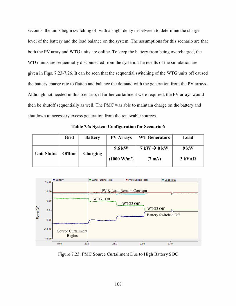
108

seconds, the units begin switching off with a slight delay in-between to determine the charge

level of the battery and the load balance on the system. The assumptions for this scenario are that

both the PV array and WTG units are online. To keep the battery from being overcharged, the

WTG units are sequentially disconnected from the system. The results of the simulation are

given in Figs. 7.23-7.26. It can be seen that the sequential switching of the WTG units off caused

the battery charge rate to flatten and balance the demand with the generation from the PV arrays.

Although not needed in this scenario, if further curtailment were required, the PV arrays would

then be shutoff sequentially as well. The PMC was able to maintain charge on the battery and

shutdown unnecessary excess generation from the renewable sources.



Unit Status Offline Charging

9.6 kW

(1000 W/m²)

7 kW 0 kW

(7 m/s)

9 kW

3 kVAR

Figure 7.23: PMC Source Curtailment Due to High Battery SOC

WTG1 Off

WTG2 Off

WTG3 Off

Battery Switched Off

PV & Load Remain Constant

Source Curtailment

Begins

109

Figure 7.24: WTG 1 Breaker Initialized by PMC

Figure 7.25: Battery SOC Change during Curtailment

WTG1 Breaker Initiated

Battery Charging

Leveled Off

110

Figure 7.26: Battery SOC Change during Curtailment

7.7 Scenario 7: Island Mode-Wind Turbine Fault Isolation

The next scenario to be investigated is impacted of a fault on the system. The microgrid is

designed such that any fault, with exception of the central battery array, can be isolated and

allow for continued operation of the remaining system. In this scenario, the terminals of the

inverter for WTG1 are faulted to ground, requiring the isolation of the WTG from the rest of

microgrid. The full system configuration for this event is given in Table 7.7. The scenario begins

at time equal to 10 seconds when the fault occurs. The WTG1 unit and the battery array supply

the fault current until the protection initiates and trips the WTG1 breaker. Although not in the

scope of this effort, it is assume that all protection devices are tuned for 3 cycle (based of 60 Hz)

clearing time. The results of the simulation are given in Figs. 7.27-7.30. It can be seen that a

surge in battery and WTG power occurred while the fault was on the line. Once the fault has

been isolated, the system returned to normal operating parameters, with one fewer WTG in

service. The system voltages drooped momentarily while the fault was active but quickly

Battery Charging

Leveled Off

111

stabilized. Since the voltage drop was less than 20% for 3 cycles, most residential loads are able

to ride through this momentarily glitch and not experience a visible loss in power.



Before

Event

Offline Discharge

9.6 kW

(1000 W/m²)

9 kW

(8 m/s)

6 kW

1 kVAR

After

Event

Offline Discharge No Change Fault on WTG1 No Change

Figure 7.27: Battery and WT Contribution to Fault Event

WTG Fault

Contributions

Battery Fault

Contributions

Fault Begins

112

Figure 7.28: System Voltage Response to Fault Event

Figure 7.29: WTG Inverter Fault Current Contribution and Isolation (after 3 cycles)

Figure 7.30: WTG PM Generator Fault Current Contribution and Isolation (after 3 cycles)

Voltage Stabilizes

in <400 ms

3 Cycling Clearing

of Fault

Rectifier Diode Current,

3 cycle clearing

Fault Begins

Fault Begins

Fault Begins

113

7.8 Scenario 8: Microgrid Resynchronization with the Grid

With the previous scenarios performed, the last event that needs to be looked at is the

interconnection of the microgrid to the macrogrid after an extended outage period. It is assumed

for this scenario that in order to prevent a large swing in power generation, only the battery array

would be online prior to resynchronization. All other sources are intentionally shut offline. It is

possible, but not shown here, that the WTG unit’s and PV arrays can come online after grid

connection is established and either recharge the battery array or back feed power to the grid.

The full system configuration for this event is given in Table 7.8. The PMC will protect from out

of phase connection to the grid by not synchronizing until both frequency, voltage, and phase

angle are within margin of the grid parameters. With the other sources offline, this is

accomplished by varying the output from the battery inverter. Once connected, the battery array

will switch back to grid connected mode of operation as discussed in Chapter 5 and reduce its

power output to zero. The results of the simulation are given in Figs. 7.31-7.33. It can be seen

that with just the battery array online and no other sources, the resynchronization is very direct.

The power output and bus voltages experience very negligible impact to the interconnection and

the switching offline of the battery array. The addition of metal-oxide varistors (MOVs), helped

to reduce the voltage spike experienced by the battery inverter and allow for a safe shutdown.



Before

Event

Offline Discharge Offline Offline

9 kW

3 kVAR

After

Event

Online Offline No Change No Change No Change

114

Figure 7.31: Change in Power Output during Resynchronization

Figure 7.32: System Voltage Change during Resynchronization

Resynchronization

Begins

Battery Ramps

Down to 0

Resynchronization

Begins

All Sources and Battery

Removed from System

115

Figure 7.33: Battery Phase Angle Change during Resynchronization

Resynchronization

Begins

Battery Transitions Offline

116

Chapter 8

Conclusions and Future Work

8.1 Research Summary

This thesis researched the design and operation of a residential microgrid for providing a

continuous source of power after a major natural disaster. The example natural disaster

referenced in this work was a hurricane striking South Florida. The system modeled in PSCAD

contained transient models of WTG’s, PV arrays, and a central battery array interconnected to an

existing distribution system network. The battery array served to act as a voltage/phase angle

reference for the renewable sources when operating in island mode. A central power

management controller (PMC) was also developed to manage these sources to ensure generation

and demand stay balanced along with the SOC of the battery array. Finally, phase-droop control

was implemented as a way to rapidly balance power changes due to the low inertia of the

inverter based generation. This complete system was simulated for various static and dynamic

scenarios where generation, load, and environmental resource were varied. The system

performed as expected with all switching related transient events settling in under 500

milliseconds and the battery able to rapidly charge or discharge depending on the system

conditions. While frequency and voltage occasionally exceeded the boundaries of a typical grid

system, they were acceptable on the microgrid due to its faster ability to respond to transients.

Energy models were also developed in MATLAB to ensure that the energy generated by the

sources met the demand of the customer throughout the day, with sufficient margin built-in. The

energy model was also used to determine the size of the energy storage array such that it could

117

operate for a sustained period of operation without generation from the renewable sources.

Overall, this thesis provided the basis for research into small microgrids to be used for ensuring

power delivery after a natural disaster. Future work can be built off this research to look at

further transient scenarios and more in-depth implementation of this proposed microgrid.

8.2 Recommended Future Work

The model developed provided the basis for studying residential microgrid scenarios. There are

several areas of study, which can be looked at to expand off this research. Proposed future

research involves looking at the communications network, expanded top level control algorithm,

and economic analysis.

8.2.1 Communications Future Work

The communications of the microgrid is important for tracking signal measurements and

determining what parameters need adjustment based off varying system conditions. Future

research in this area should look at the coordination and latency of communication from various

sources to a central controller location. This is particularly needed for geographically small

microgrids with numerous micro-generation resources. To this effect, future study into

residential microgrids should address the design of the communications infrastructure. Given the

near instantaneous response of inverter based generation to changes in source or load, the ability

to communicate this information to the controllers as quickly as possible is critical for system

stability.

118

8.2.2 Controller Future Work

This thesis provided the basis for centralized power management of a microgrid. Future work on

this model should involve expanding the capability of the PMC, particularly in grid-connected

mode of operation. There is great potential to expand the PMC to take a more active role in

providing localized real and reactive power supply into the macrogrid to help prevent outages

before they occur. A further study into the coordination of the top level controller and the

integrated communication system is also useful in determining the timing coordination between

the central controller and local controls of each inverter and protection device.

Further expanding the fidelity of the inverter controller and harmonic filter are also

recommended. The inverter model in this research provides a low fidelity model, with several

idealizations made. Revising the inverter control model will produce higher resolution transient

results. The design details should include bandwidth constraints, as well as a higher level filter

design.

8.2.3 Future Work on Economic Analysis

An economic evaluation for implementing the proposed microgrid is outside the scope of this

thesis, but remains a very important topic. Comparing the relative cost of the required hardware

for the microgrid and comparing it against the cost of a classical backup system (i.e. gas or diesel

generators) will help determine the financial viability of the project. The proposed microgrid in

this thesis has the inherent financial advantage of being a fuel-free resource, but this must

weighed against the capital cost and expected maintenance of the hardware required. In addition,

the life expectancy of the hardware is also important to evaluating the value of pursuing such an

119

implementation. A full life-cycle cost model will be needed to understand the financial benefits

or pitfalls of such a system. In addition, looking at dual uses for the microgrid such as peak

shaving or demand reduction should also be evaluated when assessing the financial viability.

8.2.4 Proposed Pilot Implementation

Implementing the microgrid in an existing residential distribution is relatively easy with respect

to hardware that is needed. All of the hardware referenced in this research is commercially

available at the time of writing the thesis. The ability to procure some or all of the hardware for

physical implementation is very practical. Two potential areas of difficulty are with respect to

the top level controls, which requires development, and utility imposed restrictions on distributed

generation. Currently the ability to implement a microgrid in a residential community is difficult

to impossible in some areas due to precautions taken by the local electric utility to ensure the

safety and reliability of electric power to their customers. Likewise, the controller for such a

microgrid requires further modeling and development before it is ready to be implemented to

scale. For future work on implementing the microgrid, it is important to engage a local utility and

encourage their participation into a pilot program to test the viability of the microgrid. If a utility

sees a financial advantage in such a system, for example reduced man power needs for line crews

after an outage, may encourage their support. The physical implementation of the proposed

microgrid could also be applied on an existing microgrid at a research university. Several options

are available when this system is ready for implementation.

120

References

[1] E. S. Blake, C.W. Landsea, and E.J. Gibney. The Deadliest, Costliest, and Most Intense

United States Tropical Cyclones from 1851 to 2010.

NOAA Technical Memorandum NWS NHC-6. National Weather Service. Aug 2011.

[2] P. Hoffman, W. Bryan, and A. Lippert. Comparing the Impacts of the 2005 and 2008

Hurricanes on U.S. Energy Infrastructure. U.S. Department of Energy. Feb 2009.

[3] J. Buyer. Technology Demonstration of a Prototype Low Carbon Monoxide Emission

Portable Generator. Consumer Product Safety Commission.

U.S. Page(s): 4. Apr 2012.

[4] P. Asmus, A. Cornelius, and C. Wheelock. Microgrids Islanded Power Grids and Distributed

Generation for Community, Commercial, and Institutional Applications. Pikes Research

Group. 4Q’09.

[5] R. Lasseter, A. Akhil, C. Marnay, J. Stephens, J. Dagle, R. Guttromson, A.S. Meliopoulous,

R. Yinger, and J. Eto. The CERTS MicroGrid Concept. Apr 2002.

[6] E. Strickland. A Microgrid That Wouldn’t Quit. http://spectrum.ieee.org/energy/the-smarter-

grid/a-microgrid-that-wouldnt-quit/0. Oct 2011.

[7] Smart Meters. Hurricane Irene Shines Spotlight on Microgrids. “http://www.smartmeters.com/the-news/2581-hurricane-irene-shines-spotlight-on-

microgrids.html

[8] S.I. Erwin. High-Tech Weapon Makers Set Sights on ‘Smart Microgrid’ Market.

http://www.nationaldefensemagazine.org/archive/2011/July/Pages/High-

TechWeaponMakersSetSightson%E2%80%98SmartMicrogrid%E2%80%99Market.aspx.

Jul 2011.

[9] H. Lammers. Microgrids: So Much More than Backup Energy. NREL Publication.

http://www.nrel.gov/news/features/feature_detail.cfm/feature_id=1980. Aug 2012.

[10] Y. Yuan, L. Wu, W. Song, and Z. Jiang. Collaborative Control of Microgrid for Emergency

Response and Disaster Relief. International Conference on Sustainable Power Generation

and Supply, 2009. SUPERGEN '09. Apr 2009.

[11] Z. Li, Y. Yuan, and F. Li. Evaluating the Reliability of Islanded Microgrid in An

Emergency Mode. UPEC 2010. Sep 2010.

[12] D. Cox. Microgrid Infrastructure Modeling for Residential Microgrids. IEEE Power

Engineering Society General Meeting, 2007. IEEE. Jul 2007.

121

[13] P. Asmus. Microgrids: Compelling Value Proposition, But Lack of Clear Policy Support.

Pike Research. http://www.pikeresearch.com/blog/articles/microgrids-compelling-value-

proposition-but-lack-of-clear-policy-support. Jan 2011.

[14] How do hurricanes form? http://spaceplace.nasa.gov/hurricanes/.

[15] Southeast Regional Climate Center. MIAMI WSCMO AIRPORT, FLORIDA

http://www.sercc.com/cgi-bin/sercc/cliMAIN.pl?fl5663.

[16] Florida 80-Meter Wind Map and Wind Resource Potential. Wind Powering America.

http://www.windpoweringamerica.gov/wind_resource_maps.asp?stateab=fl.

[17] FSU-COAPS. Florida's Missing Winds -- New Evidence Supports the Viability of

Harnessing Offshore Wind Energy in Florida.

http://www.ieses.fsu.edu/Archives/Florida-s-Missing-Winds-New-Evidence-Supports-

the-Viability-of-Harnessing-Offshore-Wind-Energy-in-Florida.

[18] South Florida Wind Resource Time of Day. http://turfgrass.com/wind/index.html.

[19] M.L. Ray, A.L. Rogers, and J.G. McGowan. Analysis of Wind Shear Models and Trends in

Different Terrains. Univ. of Massachusetts. Renewable Energy Research Laboratory.

2006.

[20] Ordinance No. 2012. Land Development Regulations. Brevard County, Florida.

http://ww3.brevardcounty.us/zoning/documents/TowerOrdinanceForWeb_02_12.pdf.

Feb 2012

[21] Does the "Sunshine" State have a sufficient solar resource to support solar energy

applications? Florida Solar Energy Center.

.http://www.fsec.ucf.edu/en/media/enews/2007/2007-04_Sunshine_state.htm. Mar. 2006.

[22] National Solar Radiation Database. September 2005 average for West Palm Beach, Florida.

http://rredc.nrel.gov/solar/old_data/nsrdb/1991-2005/.

[23] O. Tremblay, L. Dessaint, and A.I. Dekkiche. A Generic Battery Model for the Dynamic

Simulation of Hybrid Electric Vehicles. IEEE Vehicle and Propulsion Conference 2007.

Sep 2007.

[24] H. Zhag and M.Y. Chow. Comprehensive Dynamic Battery modeling for PHEV

Applications. IEEE PES General Meeting 2010. Jul 2010.

[25] F.M. Gonzalez-Longatt. Circuit Based Battery Models: A Review. 2nd

Latin American

Congress of Electrical Engineering Students. 2006

[26] Technical Manual for Sun Xtender Batteries. Concord Battery Corporation. Document No.

6-0100. Rev D. Jul 2011.

122

[27] F.M. Gonzalez-Longatt. Model of Photovoltaic Module in Matlab. 2nd

Latin American

Congress of Electrical, Electronics, and Computer Engineering Students. 2005

[28] 220 Watt Photovoltaic Module BP 3220. Datasheet. BP Solar. 2008

[29] M.G. Simões, B. Palle, S. Chakraborty, and C. Uriarte. Electrical Model Development and

Validation for Distributed Resources. National Renewable Energy Laboratory. Document

No. NREL/SR-581-41109. Apr 2007.

[30] M. Azab. Improved Circuit Model of Photovoltaic Array. International Journal of Electrical

Power and Energy Systems Engineering. Mar. 2009

[31] DC Loading of PV Powered Inverters. Advanced Energy. page 2, 2012

[32] M. Yin, G. Li, M. Zhou, and C. Zhao. Modeling of the Wind Turbine with a Permanent

Magnet Synchronous Generator for Integration. IEEE PES General Meeting 2007. Jun

2007.

[33] Hummer Wind Power Active Yaw Control Small Wind Turbine Technical Specifications.

Datasheet. Hummer Wind Power, LLC. 2009.

[34] K. Grogg. Harvesting the Wind: The Physics of Wind Turbines. Carleton College. Physics

and Astronomy Department. 2005.

[35] D.S. Parker. J.P. Dunlop, J.R. Sherwin, S.F. Barkaszi Jr., M.P. Anello, S. Durand, D.

Metzger, and J.K. Sonne. Florida Solar Energy Center.

http://www.fsec.ucf.edu/en/publications/html/FSEC-CR-1044-98/index.htm

[36] Y. Xue, J. Deng, and S. Ma. Power Flow Control of a Distributed Generation Unit in Micro-

grid. IEEE Power Electronics and Motion Control Conference, 2009. IPEMC ’09 6th

International. 2009

[37] C. Buttay. Switches Domain Map.

http://upload.wikimedia.org/wikipedia/commons/2/24/Switches_domain.svg.

[38] R.W. Erickson and D. Maksimovic. Fundamentals of Power Electronics. 2nd Edition.

Springer Science+Business Media, Inc. page(s): 282-283. 2001.

[39] H. Cha and T. Vu. Comparative Analysis of Low-pass Output Filter for Single-phase Grid-

connected Photovoltaic Inverter. APEC ’10. Page(s) 2-3. 2010.

[40] J. Doucet, D. Eggleston, and J. Shaw. DC/AC Pure Sine Wave Inverter. MQP Terms ABC

20062007. Worcerster Polytechnic Institute. 2007.

123

[41] R. Majumder, A. Ghosh, G. Ledwich, and F. Zare. Angle Droop versus Frequency Droop in

a Voltage Source Converter Based Autonomous Microgrid. Power Engineering Society

General Meeting, 2009. Annual IEEE. Jul 2009.

[42] Building Wire Copper. General Cable. Building Wire & Cable for Commercial and

Residential Applications. http://catalog.proemags.com/publication/1cfe0a62#/1cfe0a62/1.

Jan 2012.

[43] Voltage Tolerance Boundary. Pacific Gas & Electric.

http://www.pge.com/includes/docs/pdfs/mybusiness/customerservice/energystatus/power

quality/voltage_tolerance.pdf. Jan 1999.

residential microgrids for disaster recovery operations ... · 7 transient-simulation scenarios and...

Documents