residential revaluation report - thurston county, … revaluation report 2012 mass appraisal of...
TRANSCRIPT

Residential Revaluation Report
2012 Mass Appraisal of Region 9 for 2013 Property Taxes
Prepared For
Steven J. Drew
Thurston County Assessor
1
TABLE OF CONTENTS
Page No.
CERTIFICATE OF APPRAISAL ...................................................................................................................... 3
APPRAISAL TEAM ........................................................................................................................................... 4
MASS APPRAISAL CONCLUSIONS ............................................................................................................... 5
PREMISE OF THE APPRAISAL ...................................................................................................................... 6
Supporting Documents Used in the Mass Appraisal ................................................................................................. 6
CLIENT AND INTENDED USERS ................................................................................................................... 6
ASSUMPTIONS AND LIMITING CONDITIONS ........................................................................................... 7
SPECIAL ASSUMPTIONS, LIMITING, AND HYPOTHETICAL CONDITIONS ........................................ 7
JURISDICTIONAL EXCEPTION ..................................................................................................................... 7
PURPOSE AND INTENDED USE ..................................................................................................................... 8
TRUE AND FAIR VALUE ................................................................................................................................. 8
DATE OF APPRAISAL ...................................................................................................................................... 8
PROPERTY RIGHTS APPRAISED .................................................................................................................. 8
PERSONAL PROPERTY NOT INCLUDED IN THE APPRAISAL ............................................................... 8
MARKET AREA AND PROPERTIES APPRAISED ....................................................................................... 9
CITY AND NEIGHBORHOOD DESCRIPTION .............................................................................................. 9
ZONING .............................................................................................................................................................. 9
HIGHEST AND BEST USE ................................................................................................................................ 9
SCOPE OF THE APPRAISAL ......................................................................................................................... 10
REGION 9 MAP ............................................................................................................................................... 11
2
NEIGHBORHOOD MAP ................................................................................................................................. 12
RESIDENTIAL VALUATION PROCESS ...................................................................................................... 13
COST APPROACH .......................................................................................................................................... 14
Land Model Specification ............................................................................................................................................ 14
Land Model Calibration .............................................................................................................................................. 14
Multiple Regression Analysis Assumptions .............................................................................................................. 15
Validation of Region 9 Land Model ........................................................................................................................... 15
Building Cost Specification .......................................................................................................................................... 18
Construction Cost Tables ............................................................................................................................................ 18
Effective Age .................................................................................................................................................................. 19
Depreciation Rate Tables ............................................................................................................................................. 19
Condition ........................................................................................................................................................................ 20
Neighborhood Adjustment Model Specification ...................................................................................................... 21
Neighborhood Adjustment Calibration ..................................................................................................................... 21
Neighborhood Adjustment Model Validation .......................................................................................................... 22
RECONCILIATION AND CONCLUSION ..................................................................................................... 25
Summary of Inventory Statistics ................................................................................................................................ 25
APPENDIX ........................................................................................................................................................ 26
Neighborhood 10I1 – Group 01 ................................................................................................................................ 26
Neighborhood 11K1 – Group 02 ............................................................................................................................... 26
Neighborhood 11L1 – Group 03 ............................................................................................................................... 27
Neighborhood 13K1 – Group 04 ............................................................................................................................... 27
Neighborhood 17L1 – Group 05 ............................................................................................................................... 28
Neighborhood 18L1 – Group 06 ............................................................................................................................... 28
Neighborhood 15K1– Group 07 ................................................................................................................................ 29
Overall Sales Ratios for Region 9 .............................................................................................................................. 29
Multiple Regression Analysis Assumptions .............................................................................................................. 30
3
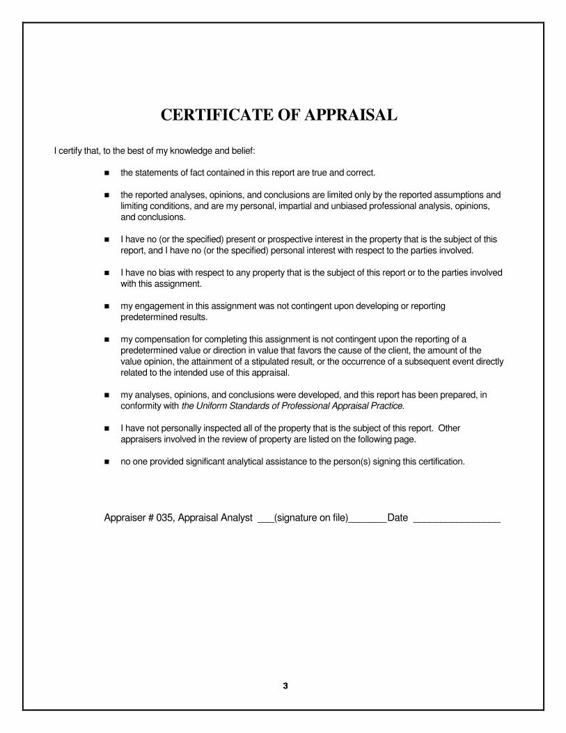
CERTIFICATE OF APPRAISAL I certify that, to the best of my knowledge and belief:
� the statements of fact contained in this report are true and correct.
� the reported analyses, opinions, and conclusions are limited only by the reported assumptions and limiting conditions, and are my personal, impartial and unbiased professional analysis, opinions, and conclusions.
� I have no (or the specified) present or prospective interest in the property that is the subject of this report, and I have no (or the specified) personal interest with respect to the parties involved.
� I have no bias with respect to any property that is the subject of this report or to the parties involved with this assignment.
� my engagement in this assignment was not contingent upon developing or reporting predetermined results.
� my compensation for completing this assignment is not contingent upon the reporting of a predetermined value or direction in value that favors the cause of the client, the amount of the value opinion, the attainment of a stipulated result, or the occurrence of a subsequent event directly related to the intended use of this appraisal.
� my analyses, opinions, and conclusions were developed, and this report has been prepared, in conformity with the Uniform Standards of Professional Appraisal Practice.
� I have not personally inspected all of the property that is the subject of this report. Other appraisers involved in the review of property are listed on the following page.
� no one provided significant analytical assistance to the person(s) signing this certification.
Appraiser # 035, Appraisal Analyst ___(signature on file)_______ Date ________________
4
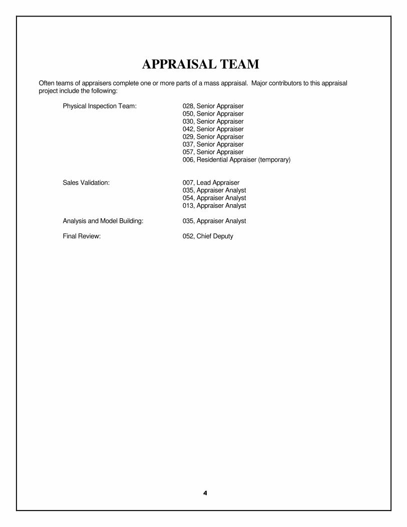
APPRAISAL TEAM
Often teams of appraisers complete one or more parts of a mass appraisal. Major contributors to this appraisal project include the following:
Physical Inspection Team: 028, Senior Appraiser
050, Senior Appraiser 030, Senior Appraiser 042, Senior Appraiser 029, Senior Appraiser
037, Senior Appraiser 057, Senior Appraiser 006, Residential Appraiser (temporary)
Sales Validation: 007, Lead Appraiser 035, Appraiser Analyst 054, Appraiser Analyst 013, Appraiser Analyst Analysis and Model Building: 035, Appraiser Analyst
Final Review: 052, Chief Deputy
5
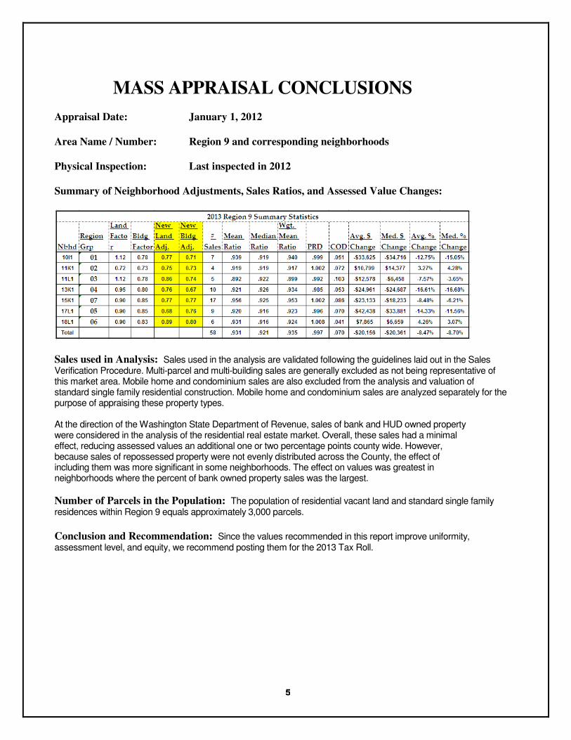
MASS APPRAISAL CONCLUSIONS
Appraisal Date: January 1, 2012
Area Name / Number: Region 9 and corresponding neighborhoods
Physical Inspection: Last inspected in 2012
Summary of Neighborhood Adjustments, Sales Ratios, and Assessed Value Changes:
Sales – Improved Valuation Change
Sales used in Analysis: Sales used in the analysis are validated following the guidelines laid out in the Sales Verification Procedure. Multi-parcel and multi-building sales are generally excluded as not being representative of this market area. Mobile home and condominium sales are also excluded from the analysis and valuation of standard single family residential construction. Mobile home and condominium sales are analyzed separately for the purpose of appraising these property types. At the direction of the Washington State Department of Revenue, sales of bank and HUD owned property were considered in the analysis of the residential real estate market. Overall, these sales had a minimal effect, reducing assessed values an additional one or two percentage points county wide. However, because sales of repossessed property were not evenly distributed across the County, the effect of including them was more significant in some neighborhoods. The effect on values was greatest in neighborhoods where the percent of bank owned property sales was the largest.
Number of Parcels in the Population: The population of residential vacant land and standard single family residences within Region 9 equals approximately 3,000 parcels.
Conclusion and Recommendation: Since the values recommended in this report improve uniformity, assessment level, and equity, we recommend posting them for the 2013 Tax Roll.
6
PREMISE OF THE APPRAISAL Supporting Documents Used in the Mass Appraisal
"A mass appraisal is the process of valuing a universe of properties as of a given date using standard methodology, employing common data, and allowing for statistical testing."
1
A mass appraisal for ad valorem taxes is a complicated process involving large amounts of data, gathered and analyzed by teams of appraisers. We do not intend this document to be a self-contained documentation of the mass appraisal but to summarize our methods, data, and to guide the reader to other documents or files, upon which we relied. These documents may include the following:
• Individual property records maintained in a computer database
• Sales ratios and other statistical studies
• Market studies
• Model building documents
• Real estate sales database.
• Previous studies and reports filed in our office.
• Assessor’s manuals for data collection analysis.
• Revaluation and sales verification manuals
• Property Tax Advisory Publications by the Washington State Dept. of Revenue.
• Title 84 RCW Property Tax Laws (Washington State Law)
• WAC 458 (Washington Administrative Code)
The Appraisal Standards Board of the Appraisal Foundation annually publishes the Uniform Standards of
Professional Appraisal Practice (USPAP). These standards are written by appraisers to regulate their profession and are the minimum standards for the conduct of property appraisal in the United States. They cover real, personal, and business property. We rely upon these standards in the development and reporting of our assessed values.
CLIENT AND INTENDED USERS
This report was prepared for Steven J. Drew, Thurston County Assessor. Other intended users include the County Board of Equalization and the State Board of Tax Appeals.
1 USPAP, Appraisal Standards Board of the Appraisal Foundation, p. 3
7
ASSUMPTIONS AND LIMITING CONDITIONS
The Appraisal Report, of which this statement is a part, is expressly subject to the following conditions: This revaluation is a mass appraisal assignment resulting in conclusions of market value. No one should rely on this study for any purpose other than administration and distribution of ad valorem taxation. The opinion of value on any parcel may not be applicable for any use other than ad valorem taxation. That the maps and drawings in this report are included to assist the reader in visualizing the property; however, no responsibility is assumed as to their exactness. That the legal description as given is assumed correct. No survey or search of title of the property has been made for this report, and no responsibility for legal matters is assumed. The report assumes good merchantable title and any liens or encumbrances that may exist have been disregarded. The opinions and values shown in the report apply to the subject parcels only. The assessors made no attempt to relate the conclusions of this report to any other revaluations, past, present, or future. The assumptions governing the use of multiple linear regression analysis have been met unless otherwise stated. Unless otherwise stated in this report, the existence of hazardous substances, including without limitation asbestos, polychlorinated biphenyl, petroleum leakage, or agricultural chemicals, which may or may not be present on the property, or other environmental conditions, were not called to the attention of nor did the appraiser become aware of such during the appraiser's inspection. The appraiser has no knowledge of the existence of such materials on or in the property unless otherwise stated. The appraiser, however, is not qualified to test such substances or conditions. If the presence of such substances, such as asbestos, urea formaldehyde foam insulation, or other hazardous substances or environmental conditions, may affect the value of the property, the value estimates is predicated on the assumption that there is no such condition on or in the property or in such proximity thereto that it would cause a loss in value. No responsibility is assumed for any such conditions, or for any expertise or engineering knowledge required to discover them.
SPECIAL ASSUMPTIONS, LIMITING, AND
HYPOTHETICAL CONDITIONS
We assume that none of the subject land is contaminated or that any contamination would affect the value except as shown in individual property records or otherwise stated.
Because of budget restraints, we have not inspected all comparable sales. We have inspected the interiors of only a small percentage of the properties.
JURISDICTIONAL EXCEPTION
Washington exempts all or a portion of the market value on specific types of property including “open space,” agricultural, forest, home improvement, and some low-income housing.

8
PURPOSE AND INTENDED USE
The intended use of this appraisal is for administration of ad valorem taxation. After certification by the Assessor, these values will be used as the basis for assessment of real estate taxes payable in 2013. We do not intend the values to be used for or relied upon for any other purpose.
This report serves as a record of the revaluation which is subject to review and change by the County Board of Equalization, the Washington State Board of Tax Appeals, and the courts.
TRUE AND FAIR VALUE
The basis of all assessments is the true and fair value of property. True and fair value means market value (Spokane etc. R. Company v. Spokane County, 75 Wash. 72 (1913): Mason County, 62 Wn. 2d (1963); AGO 57-58, No. 1/8/57; AGO 65-66, No. 65, 12/31/65)
The true and fair value of a property in money for property tax valuation purposes is its "market value" or amount of money a buyer willing but not obligated to buy would pay for it to a seller willing but not obligated to sell. In arriving at a determination of such value, the assessing officer can consider only those factors which can within reason be said to affect the price in negotiations between a willing purchaser and a willing seller, and he must consider all of such factors. (AGO 65,66, No. 65, 12/31/65)
DATE OF APPRAISAL
Properties are appraised as of January 1, 2012.
This report was completed June 1, 2012.
PROPERTY RIGHTS APPRAISED
This appraisal is of the fee simple interest in the real property. The fee simple estate is the absolute ownership unencumbered by any other interest or estate, subject only to the limitations imposed by the governmental powers of taxation, eminent domain, police power, and escheat.
2
PERSONAL PROPERTY NOT INCLUDED IN THE
APPRAISAL
No personal property was included in the value. Fixtures are generally accepted as real property. Business value is intangible personal property and it is not appraised.
2 The Dictionary of Real Estate Appraisal. 3d ed. Appraisal Institute, p.140
9
MARKET AREA AND PROPERTIES APPRAISED
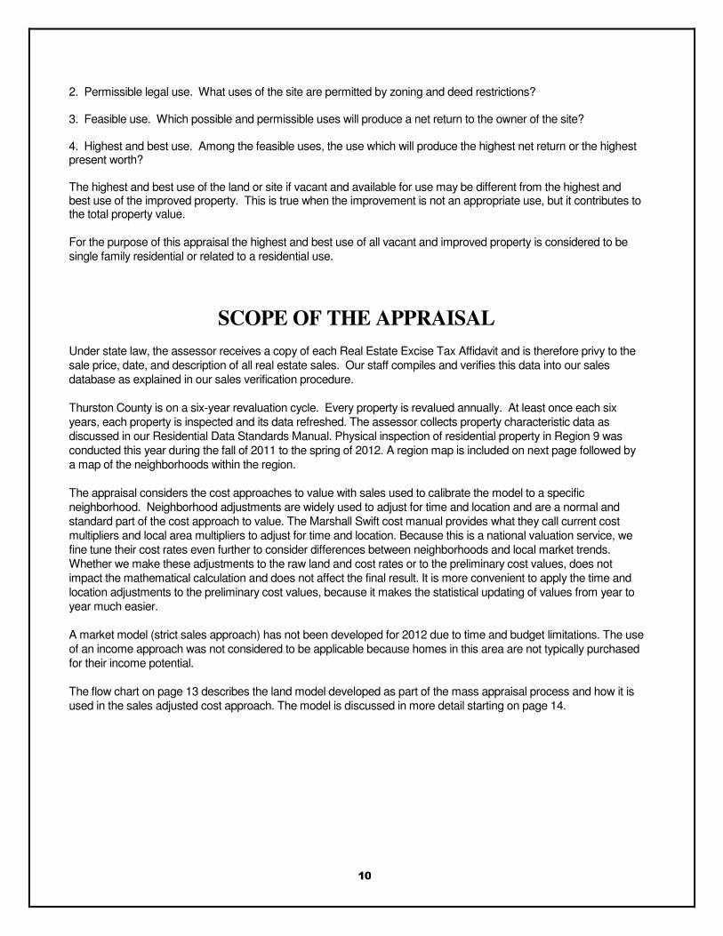
The subject of this mass appraisal is the residential property (excluding mobile homes and condominiums) contained in the market area designated as Region 9. Regions are generally influenced by the same broad market trends. This area includes approximately 3,000 properties and is shown on the map on page 11 of this report.
Our property records contain photographs, sketches, legal descriptions and other characteristics of land and buildings on each property.
CITY AND NEIGHBORHOOD DESCRIPTION
Region 9 is in central Thurston County just south of the City of Tumwater and its urban growth area. Its western border lies just past Little Rock Road. Its northern boundary runs primarily along 93
rd Avenue. Its
eastern edge is just past Tempo Lake. And, southern boundary line runs primarily along Offutt Lake/123rd
west to Maytown Road, except west of I-5 where it extends just past 140th Avenue.
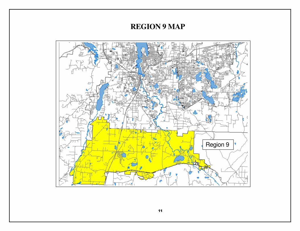
This region is further broken into 7 residential neighborhoods that are designed to reflect similar land and building characteristics and neighborhood amenities. Due to the limited number of sales sometimes these neighbors are grouped for appraisal purposes. The neighborhoods and their codes are shown on page 12. They are all considered to be stable in terms of the life cycle of a neighborhood.
ZONING
Thurston County exercises jurisdiction over land use and community planning. The regulations for use and development can be found in its ordinances. We show property zoning as a land characteristic on our digital maps.
HIGHEST AND BEST USE
True and fair value -- Highest and best use. Unless specifically provided otherwise by statute, all property shall be valued on the basis of its highest and best use for assessment purposes. Highest and best use is the most profitable, likely use to which a property can be put. It is the use which will yield the highest return on the owner's investment. Any reasonable use to which the property may be put may be taken into consideration and if it is peculiarly adapted to some particular use, that fact may be taken into consideration. Uses that are within the realm of possibility, but not reasonably probable of occurrence, shall not be considered in valuing property at its highest and best use. [WAC 458-07-30 (3)]
The highest and best use concept is based upon traditional appraisal theory and reflects the attitudes of typical buyers and sellers. The market sets the highest and best use based on the theory of wealth maximization for the owner with consideration given to community goals. To estimate highest and best use, four elements are considered: 1. Possible use. What uses of the site in question are physically possible?
10
2. Permissible legal use. What uses of the site are permitted by zoning and deed restrictions? 3. Feasible use. Which possible and permissible uses will produce a net return to the owner of the site? 4. Highest and best use. Among the feasible uses, the use which will produce the highest net return or the highest present worth? The highest and best use of the land or site if vacant and available for use may be different from the highest and best use of the improved property. This is true when the improvement is not an appropriate use, but it contributes to the total property value. For the purpose of this appraisal the highest and best use of all vacant and improved property is considered to be single family residential or related to a residential use.
SCOPE OF THE APPRAISAL
Under state law, the assessor receives a copy of each Real Estate Excise Tax Affidavit and is therefore privy to the sale price, date, and description of all real estate sales. Our staff compiles and verifies this data into our sales database as explained in our sales verification procedure.
Thurston County is on a six-year revaluation cycle. Every property is revalued annually. At least once each six years, each property is inspected and its data refreshed. The assessor collects property characteristic data as discussed in our Residential Data Standards Manual. Physical inspection of residential property in Region 9 was conducted this year during the fall of 2011 to the spring of 2012. A region map is included on next page followed by a map of the neighborhoods within the region.
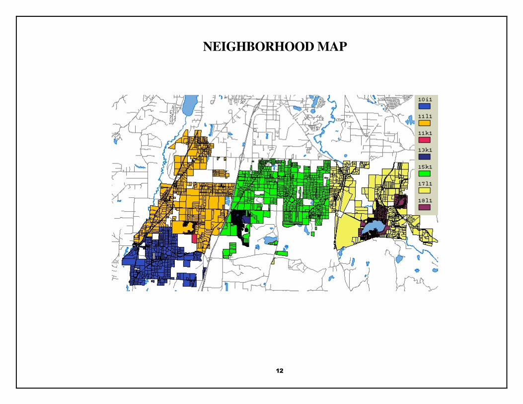
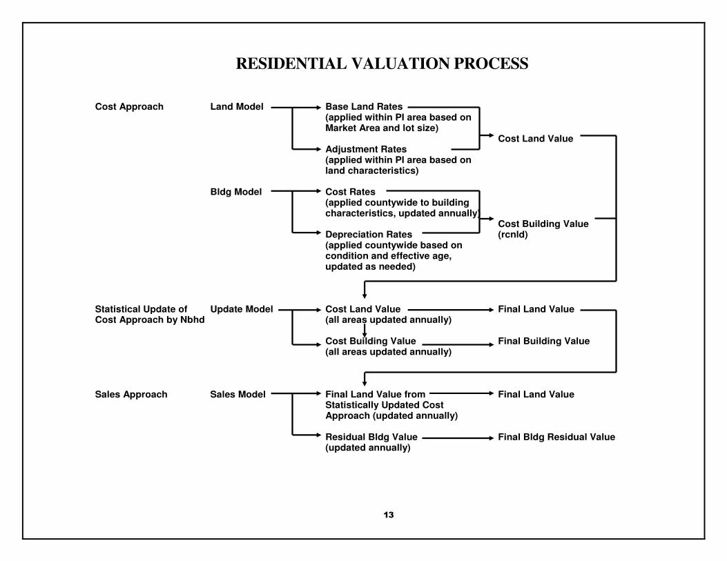
The appraisal considers the cost approaches to value with sales used to calibrate the model to a specific neighborhood. Neighborhood adjustments are widely used to adjust for time and location and are a normal and standard part of the cost approach to value. The Marshall Swift cost manual provides what they call current cost multipliers and local area multipliers to adjust for time and location. Because this is a national valuation service, we fine tune their cost rates even further to consider differences between neighborhoods and local market trends. Whether we make these adjustments to the raw land and cost rates or to the preliminary cost values, does not impact the mathematical calculation and does not affect the final result. It is more convenient to apply the time and location adjustments to the preliminary cost values, because it makes the statistical updating of values from year to year much easier.
A market model (strict sales approach) has not been developed for 2012 due to time and budget limitations. The use of an income approach was not considered to be applicable because homes in this area are not typically purchased for their income potential.
The flow chart on page 13 describes the land model developed as part of the mass appraisal process and how it is used in the sales adjusted cost approach. The model is discussed in more detail starting on page 14.
11
REGION 9 MAP
Region 9
12
NEIGHBORHOOD MAP
13
RESIDENTIAL VALUATION PROCESS
Cost Approach Land Model Base Land Rates (applied within PI area based on
Market Area and lot size) Cost Land Value
Adjustment Rates (applied within PI area based on
land characteristics) Bldg Model Cost Rates (applied countywide to building
characteristics, updated annually) Cost Building Value Depreciation Rates (rcnld) (applied countywide based on
condition and effective age, updated as needed)
Statistical Update of Update Model Cost Land Value Final Land Value Cost Approach by Nbhd (all areas updated annually) Cost Building Value Final Building Value (all areas updated annually) Sales Approach Sales Model Final Land Value from Final Land Value Statistically Updated Cost
Approach (updated annually)
Residual Bldg Value Final Bldg Residual Value (updated annually)
14
COST APPROACH
Land Model Specification
• A multiplicative model format is used in the development of base land rates and adjustment rates.
• Land Model Format: LV = b0 X SQFT
b1 X LINVIEW
b2 X b3
LI3 X b4
LI4 X b5
LI5 X . . .
Where: Continuous Variables = SQFT, LINVIEW Binary Variables LI3, LI4, LI5 . . . = Land Influences (i.e. – region, view, wetlands, etc.) b0, b1, b2, b3, b4, b5 . . . = Regression Coefficients
• Note: Approval to deviate from our normal process to develop and update the land model for the Physical Inspection Area was obtained from the Department of Revenue. The model from the previous cycle was kept in place and statistically updated as part of the neighborhood calibration process.
Land Model Calibration
• Multiplicative model calibrated using log-linear MRA
• Logarithms are used to convert a multiplicative equation to a linear form.
Standard Multiplicative form: SP/SQFT = a * SQFTb * c
NBHD * . . .
Log Linear form: LN(SP/SQFT) = LN(a) + (b * LN(SQFT)) + (LN(c) * NBHD) + . . . • Log Linear form has the same form as a standard linear equation:
Linear equation: Y = a + (b * X) + (c * Z) • We can then calibrate the Log-Linear form using standard multiple regression analysis. • The calibrated model is then converted back to its Standard Multiplicative form by applying the anti-log
function.
EXP[LN(SP/SQFT)] = EXP[LN(a) + (b * LN(SQFT))] * RegionAdj
• Region 9 Land Model – see Region 9 work files for model coefficients and other output.
15
Multiple Regression Analysis Assumptions
Multiple regression analysis is based on several assumptions regarding the data going into the model and the output from the calibration process. These assumptions are validated to determine the accuracy of the model and identify any limitations that may exist. A detailed discussion of the MRA assumptions is included in the Appendix.
Validation of Region 9 Land Model
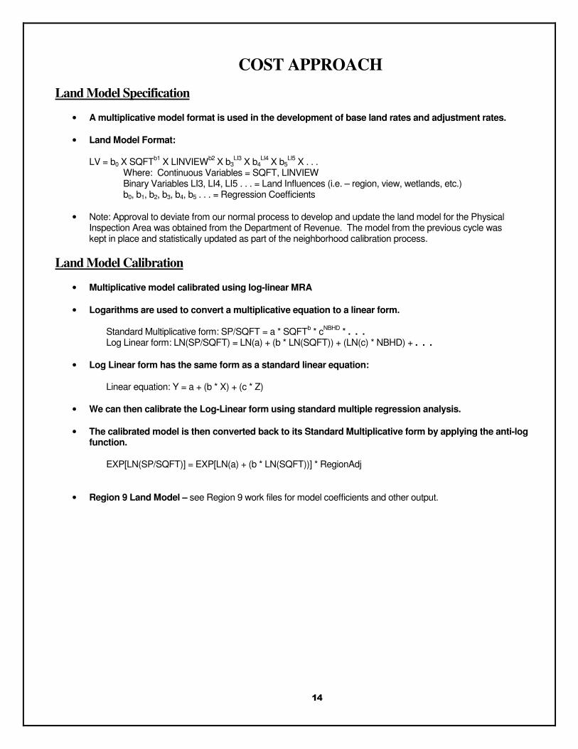
Normal Distribution of the Residual Errors
• Total number of sales = 1733 (from 1/1/03 – 12/31/05 trended to 1/1/06) • Region 09 sales = 26 • The residual errors are for the most part normally distributed. • While the frequency distribution illustrates output from the square foot land model, similar results were
obtained for the acreage model.
16
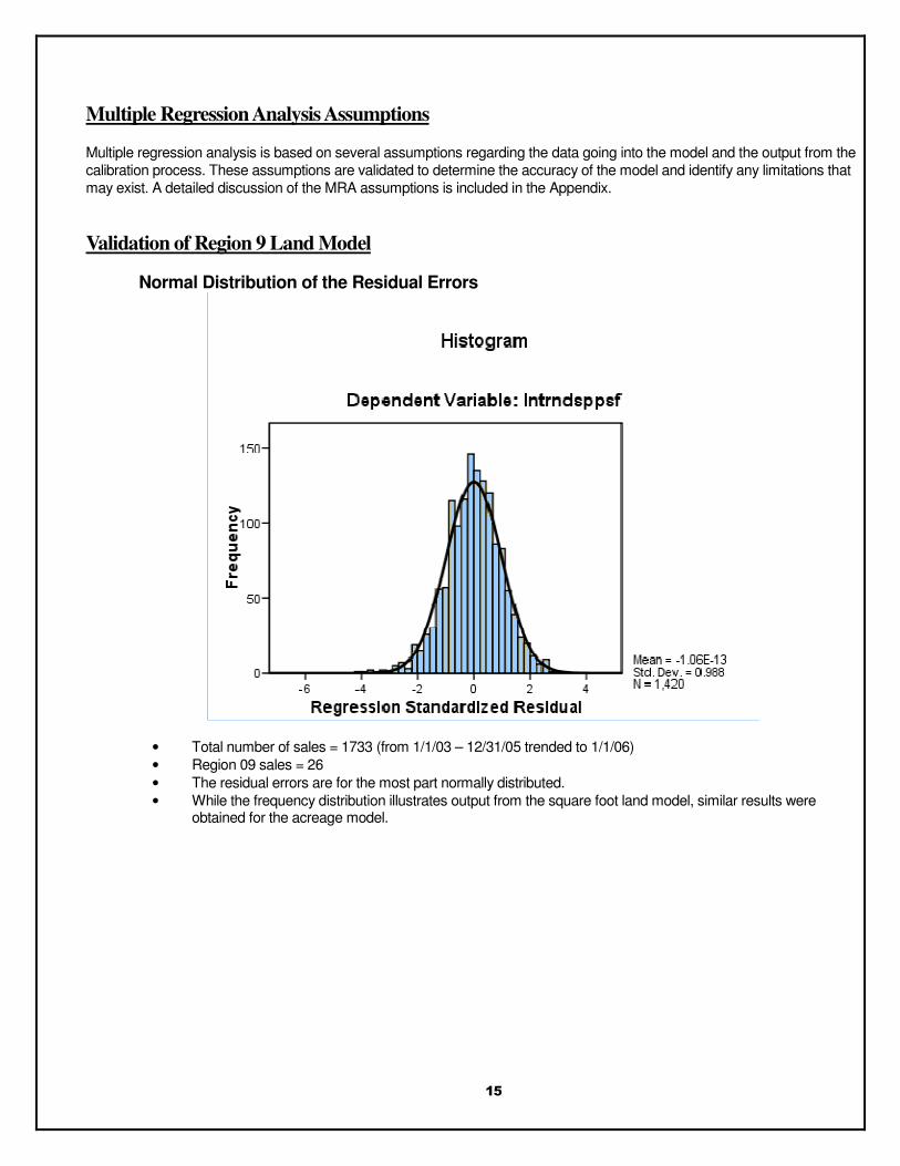
Constant Variance of the Residual Errors
• The residual errors are for the most part are distributed evenly along the range of values. • Similar results were obtained for the acreage model.
Comparison of Predicted and Actual Sale Price per Sq. Ft.
• The values predicted by the model accurately reflects actual trended sale prices . • Similar results were obtained for the acreage model.
17
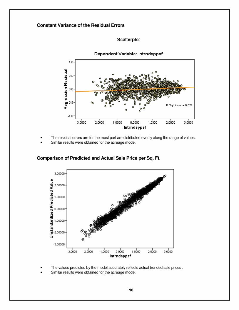
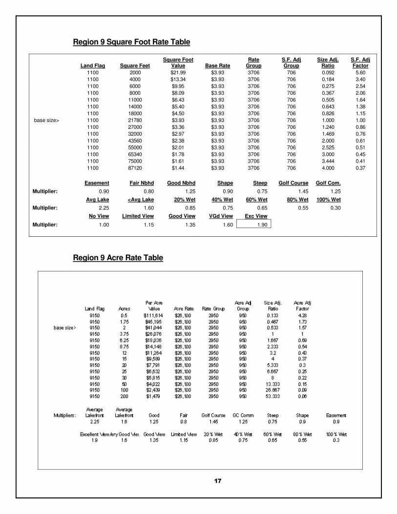
Region 9 Square Foot Rate Table
Land Flag Square Feet Square Foot
Value Base Rate Rate
Group S.F. Adj Group
Size Adj. Ratio
S.F. Adj Factor
1100 2000 $21.99 $3.93 3706 706 0.092 5.60
1100 4000 $13.34 $3.93 3706 706 0.184 3.40
1100 6000 $9.95 $3.93 3706 706 0.275 2.54
1100 8000 $8.09 $3.93 3706 706 0.367 2.06
1100 11000 $6.43 $3.93 3706 706 0.505 1.64
1100 14000 $5.40 $3.93 3706 706 0.643 1.38
1100 18000 $4.50 $3.93 3706 706 0.826 1.15
base size> 1100 21780 $3.93 $3.93 3706 706 1.000 1.00
1100 27000 $3.36 $3.93 3706 706 1.240 0.86
1100 32000 $2.97 $3.93 3706 706 1.469 0.76
1100 43560 $2.38 $3.93 3706 706 2.000 0.61
1100 55000 $2.01 $3.93 3706 706 2.525 0.51
1100 65340 $1.78 $3.93 3706 706 3.000 0.45
1100 75000 $1.61 $3.93 3706 706 3.444 0.41
1100 87120 $1.44 $3.93 3706 706 4.000 0.37
Easement Fair Nbhd Good Nbhd Shape Steep Golf Course Golf Com.
Multiplier: 0.90 0.80 1.25 0.90 0.75 1.45 1.25
Avg Lake <Avg Lake 20% Wet 40% Wet 60% Wet 80% Wet 100% Wet
Multiplier: 2.25 1.60 0.85 0.75 0.65 0.55 0.30
No View Limited View Good View VGd View Exc View
Multiplier: 1.00 1.15 1.35 1.60 1.90
Region 9 Acre Rate Table
18
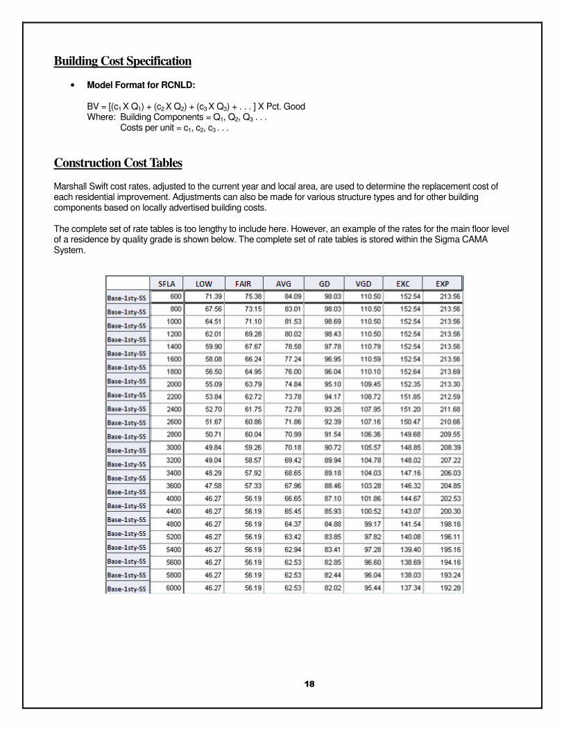
Building Cost Specification
• Model Format for RCNLD: BV = [(c1 X Q1) + (c2 X Q2) + (c3 X Q3) + . . . ] X Pct. Good Where: Building Components = Q1, Q2, Q3 . . . Costs per unit = c1, c2, c3 . . .
Construction Cost Tables
Marshall Swift cost rates, adjusted to the current year and local area, are used to determine the replacement cost of each residential improvement. Adjustments can also be made for various structure types and for other building components based on locally advertised building costs. The complete set of rate tables is too lengthy to include here. However, an example of the rates for the main floor level of a residence by quality grade is shown below. The complete set of rate tables is stored within the Sigma CAMA System.
19
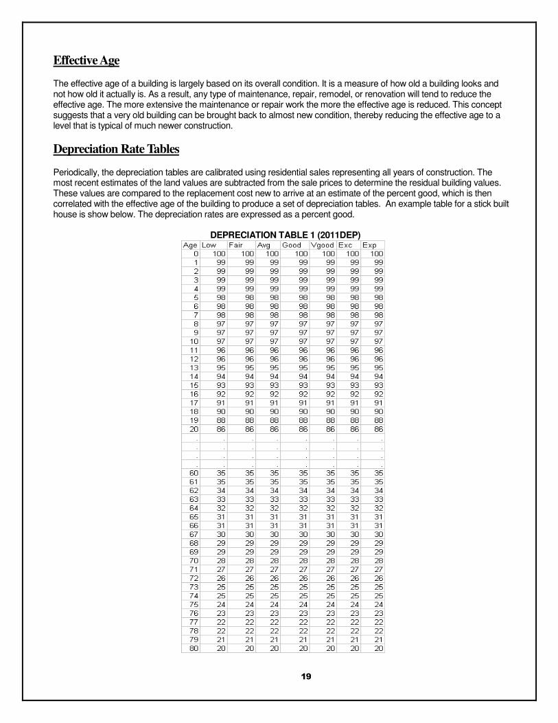
Effective Age
The effective age of a building is largely based on its overall condition. It is a measure of how old a building looks and not how old it actually is. As a result, any type of maintenance, repair, remodel, or renovation will tend to reduce the effective age. The more extensive the maintenance or repair work the more the effective age is reduced. This concept suggests that a very old building can be brought back to almost new condition, thereby reducing the effective age to a level that is typical of much newer construction.
Depreciation Rate Tables
Periodically, the depreciation tables are calibrated using residential sales representing all years of construction. The most recent estimates of the land values are subtracted from the sale prices to determine the residual building values. These values are compared to the replacement cost new to arrive at an estimate of the percent good, which is then correlated with the effective age of the building to produce a set of depreciation tables. An example table for a stick built house is show below. The depreciation rates are expressed as a percent good.
DEPRECIATION TABLE 1 (2011DEP)

20
The graph below shows the relationship between the percent good, actual age, and effective age.
Condition
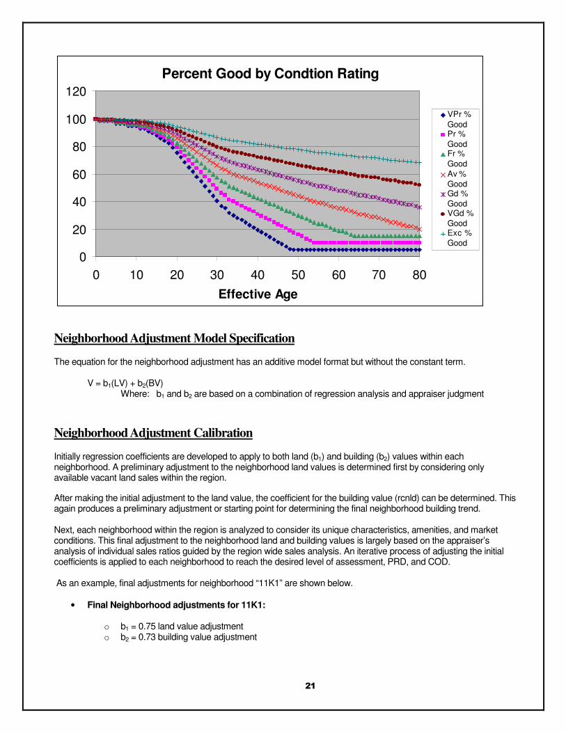
Because many properties are in better or worse condition than what is typical for their age, we need a method to adjust the depreciation rate accordingly. There are two ways to accomplish this. One is to adjust the effective age and the other is to adjust the condition rating to raise or lower the amount of depreciation that is applied. Adjusting the effective age would involve a fairly complex set of instructions and calculations for different situations that may be encountered. Minor remodels, major renovations, and building additions would require different adjustment techniques. Even with these procedures in place, there would be substantial appraiser judgment involved that would open the door for inconsistencies in the way effective age is determined and depreciation is applied. A better method is to establish guidelines for determining the condition rating to apply to each property. In general, if an improvement to a parcel of land is typical for its age and has received average maintenance, it would be considered to be in average condition. If the improvement has had less than average maintenance, it will be in less than average condition. If the improvement has received better than average maintenance, it will be in better than average condition. The following graph shows the effect that the condition rating has on the percent good curve. It summarizes the relationship between effective age, building condition, and the rate of depreciation.
Percent Good
0
20
40
60
80
100
120
0 10 20 30 40 50 60 70 80 Eff. Age
0 10 42 87 103 114 123 130 140 Actual Age
21
Percent Good by Condtion Rating
0
20
40
60
80
100
120
0 10 20 30 40 50 60 70 80
Effective Age
VPr %
GoodPr %
GoodFr %
GoodAv %GoodGd %GoodVGd %GoodExc %Good
Neighborhood Adjustment Model Specification
The equation for the neighborhood adjustment has an additive model format but without the constant term.
V = b1(LV) + b2(BV) Where: b1 and b2 are based on a combination of regression analysis and appraiser judgment
Neighborhood Adjustment Calibration
Initially regression coefficients are developed to apply to both land (b1) and building (b2) values within each neighborhood. A preliminary adjustment to the neighborhood land values is determined first by considering only available vacant land sales within the region.
After making the initial adjustment to the land value, the coefficient for the building value (rcnld) can be determined. This again produces a preliminary adjustment or starting point for determining the final neighborhood building trend. Next, each neighborhood within the region is analyzed to consider its unique characteristics, amenities, and market conditions. This final adjustment to the neighborhood land and building values is largely based on the appraiser’s analysis of individual sales ratios guided by the region wide sales analysis. An iterative process of adjusting the initial coefficients is applied to each neighborhood to reach the desired level of assessment, PRD, and COD. As an example, final adjustments for neighborhood “11K1” are shown below.
• Final Neighborhood adjustments for 11K1:
o b1 = 0.75 land value adjustment o b2 = 0.73 building value adjustment
22
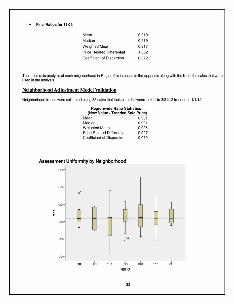
• Final Ratios for 11K1:
Mean 0.919
Median 0.919
Weighted Mean 0.917
Price Related Differential 1.002
Coefficient of Dispersion 0.072
The sales ratio analysis of each neighborhood in Region 9 is included in the appendix along with the list of the sales that were used in the analysis.
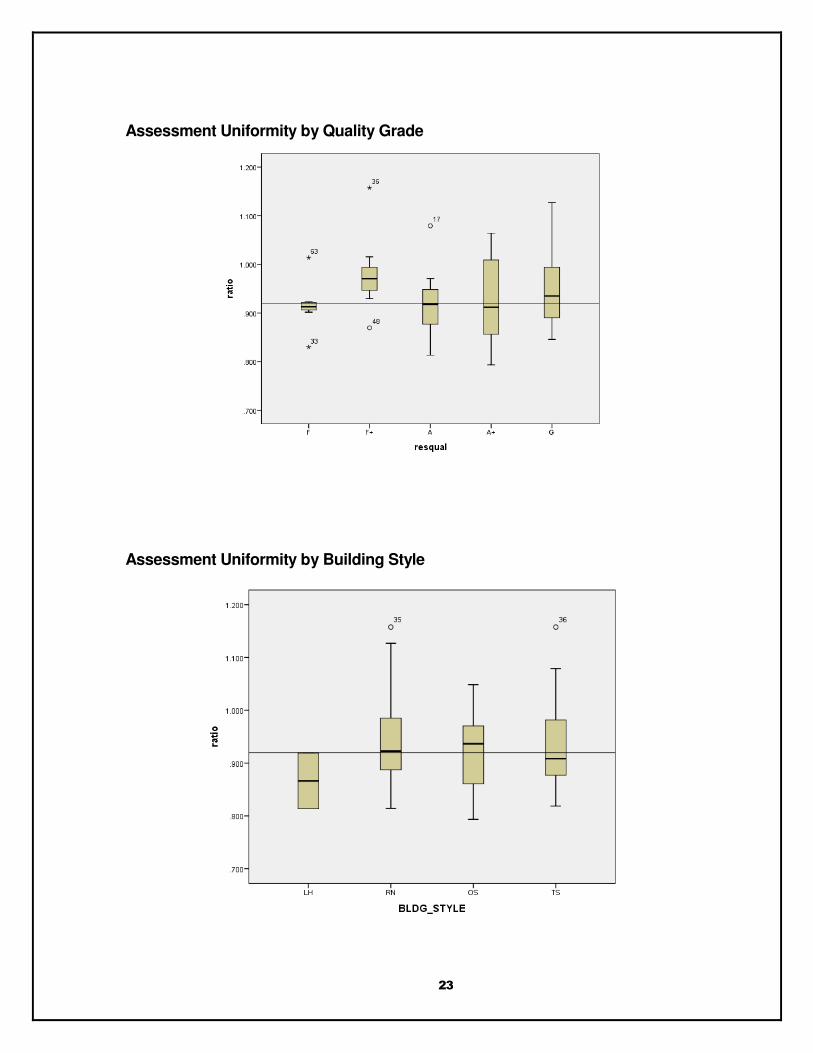
Neighborhood Adjustment Model Validation
Neighborhood trends were calibrated using 58 sales that took place between 1/1/11 to 3/31/12 trended to 1/1/12.
Regionwide Ratio Statistics (New Value / Trended Sale Price)
Mean 0.931
Median 0.921
Weighted Mean 0.935
Price Related Differential 0.997
Coefficient of Dispersion 0.070
Assessment Uniformity by Neighborhood
23
Assessment Uniformity by Quality Grade
Assessment Uniformity by Building Style
24
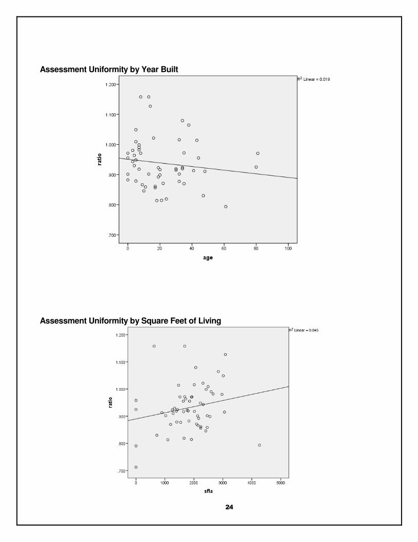
Assessment Uniformity by Year Built
Assessment Uniformity by Square Feet of Living

25
RECONCILIATION AND CONCLUSION
Considering the quantity and quality of data and the reliability of the various models as shown in the performance tests above, we have concluded that the Sales Adjusted Cost Approach produces an accurate estimate of market value.
Summary of Inventory Statistics
Region 09 Inventory Statistics
NBHD STATS FINAL VALUE chgamt chgperc (%) chglnd (%) chgimp (%)
10I1 Mean $195,746 -$26,628 -13.05 -3.98 -21.06
Median $199,950 -$24,200 -13.48 -5.04 -16.75
11K1 Mean $351,722 $9,814 2.25 5.75 -5.18
Median $363,300 $10,150 3.64 5.55 -7.55
11L1 Mean $202,780 -$16,698 -6.79 1.84 -13.03
Median $198,850 -$11,175 -5.82 -1.28 -13.24
13K1 Mean $114,352 -$21,877 -16.74 -6.93 -20.04
Median $125,650 -$23,250 -16.67 -13.96 -20.00
15K1 Mean $236,505 -$19,965 -8.03 -2.55 -13.75
Median $239,800 -$20,300 -9.42 -5.47 -14.45
17L1 Mean $168,032 -$31,417 -17.89 -9.05 -24.17
Median $159,800 -$28,650 -16.76 -7.78 -24.45
18L1 Mean $152,748 -$1,113 -0.10 0.84 -1.13
Median $157,150 -$775 -1.10 -0.62 -1.11
Total Mean $188,875 -$18,232 -9.59 -2.60 -14.73
Median $177,600 -$18,150 -10.66 -4.73 -14.49
26
APPENDIX
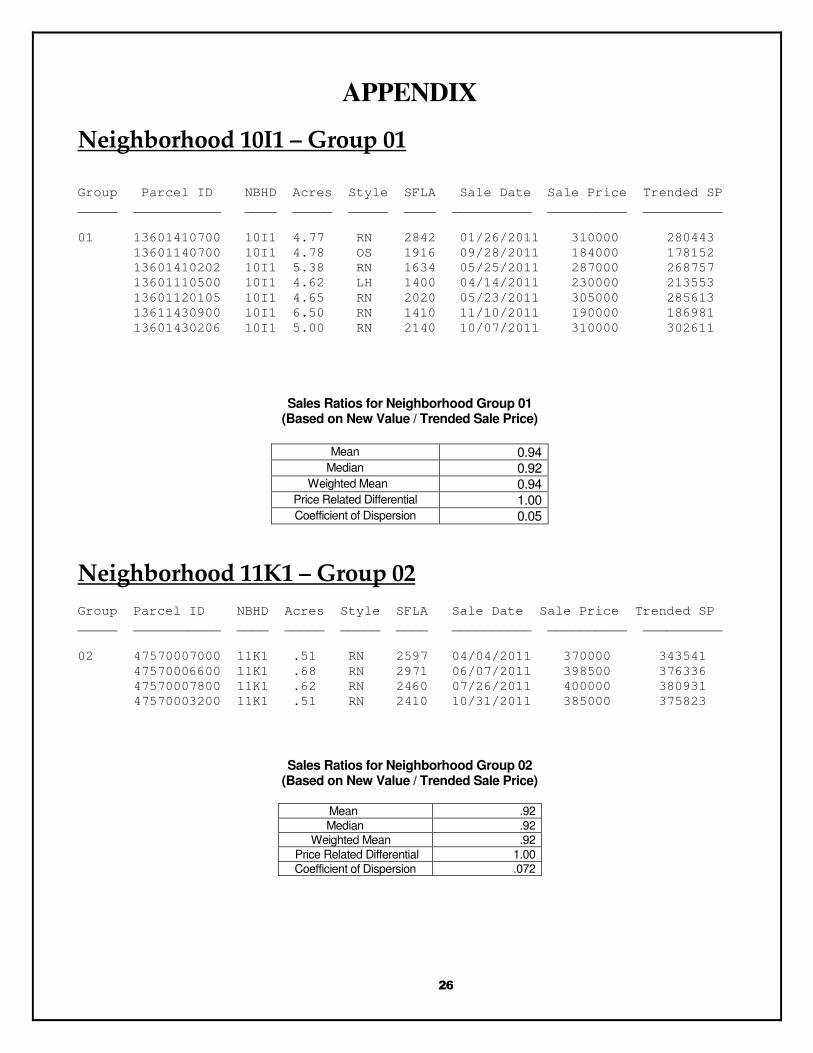
Neighborhood 10I1 – Group 01
Group Parcel ID NBHD Acres Style SFLA Sale Date Sale Price Trended SP
_____ ___________ ____ _____ _____ ____ __________ __________ __________
01 13601410700 10I1 4.77 RN 2842 01/26/2011 310000 280443
13601140700 10I1 4.78 OS 1916 09/28/2011 184000 178152
13601410202 10I1 5.38 RN 1634 05/25/2011 287000 268757
13601110500 10I1 4.62 LH 1400 04/14/2011 230000 213553
13601120105 10I1 4.65 RN 2020 05/23/2011 305000 285613
13611430900 10I1 6.50 RN 1410 11/10/2011 190000 186981
13601430206 10I1 5.00 RN 2140 10/07/2011 310000 302611
Sales Ratios for Neighborhood Group 01 (Based on New Value / Trended Sale Price)
Neighborhood 11K1 – Group 02
Group Parcel ID NBHD Acres Style SFLA Sale Date Sale Price Trended SP
_____ ___________ ____ _____ _____ ____ __________ __________ __________
02 47570007000 11K1 .51 RN 2597 04/04/2011 370000 343541
47570006600 11K1 .68 RN 2971 06/07/2011 398500 376336
47570007800 11K1 .62 RN 2460 07/26/2011 400000 380931
47570003200 11K1 .51 RN 2410 10/31/2011 385000 375823
Sales Ratios for Neighborhood Group 02 (Based on New Value / Trended Sale Price)
Mean .92 Median .92
Weighted Mean .92 Price Related Differential 1.00 Coefficient of Dispersion .072
Mean 0.94 Median 0.92
Weighted Mean 0.94 Price Related Differential 1.00 Coefficient of Dispersion 0.05

27
Neighborhood 11L1 – Group 03
Group Parcel ID NBHD Acres Style SFLA Sale Date Sale Price Trended SP
_____ ___________ ____ _____ _____ ____ __________ __________ __________
03 12728230700 11L1 3.13 TS 2064 08/12/2011 190500 182932
13736340500 11L1 9.90 OS 1424 03/17/2011 200000 184109
12717320402 11L1 2.45 RN 1764 06/27/2011 280500 264899
12719240200 11L1 8.15 TS 1661 09/14/2011 254200 246121
12730220101 11L1 4.96 0 02/25/2011 145000 129210
Sales Ratios for Neighborhood Group 01 (Based on New Value / Trended Sale Price)
Neighborhood 13K1 – Group 04
Group Parcel ID NBHD Acres Style SFLA Sale Date Sale Price Trended SP
_____ ___________ ____ _____ _____ ____ __________ __________ __________
04 72792101800 13K1 .48 RN 2013 09/29/2011 192000 185898
72771500900 13K1 .31 RN 1517 06/16/2011 175000 165267
72791806800 13K1 .73 TS 1933 08/29/2011 200000 192054
72760601900 13K1 .25 RN 1716 10/28/2011 175000 170829
72761300300 13K1 .26 RN 1331 07/28/2011 151200 143992
72791805300 13K1 .32 RN 1254 09/20/2011 149900 145136
72760403700 13K1 .27 RN 1284 11/09/2011 109099 107365
72792001300 13K1 .29 RN 1024 10/13/2011 109000 106402
72750402300 13K1 .24 RN 720 05/06/2011 108000 101135
72750102800 13K1 .90 0 02/14/2011 110000 98021
Sales Ratios for Neighborhood Group 04 (Based on New Value / Trended Sale Price)
Mean 0.92 Median 0.93
Weighted Mean 0.93 Price Related Differential 0.99
Coefficient of Dispersion 0.05
Mean 0.89 Median 0.92
Weighted Mean 0.90 Price Related Differential 0.99 Coefficient of Dispersion 0.10
28
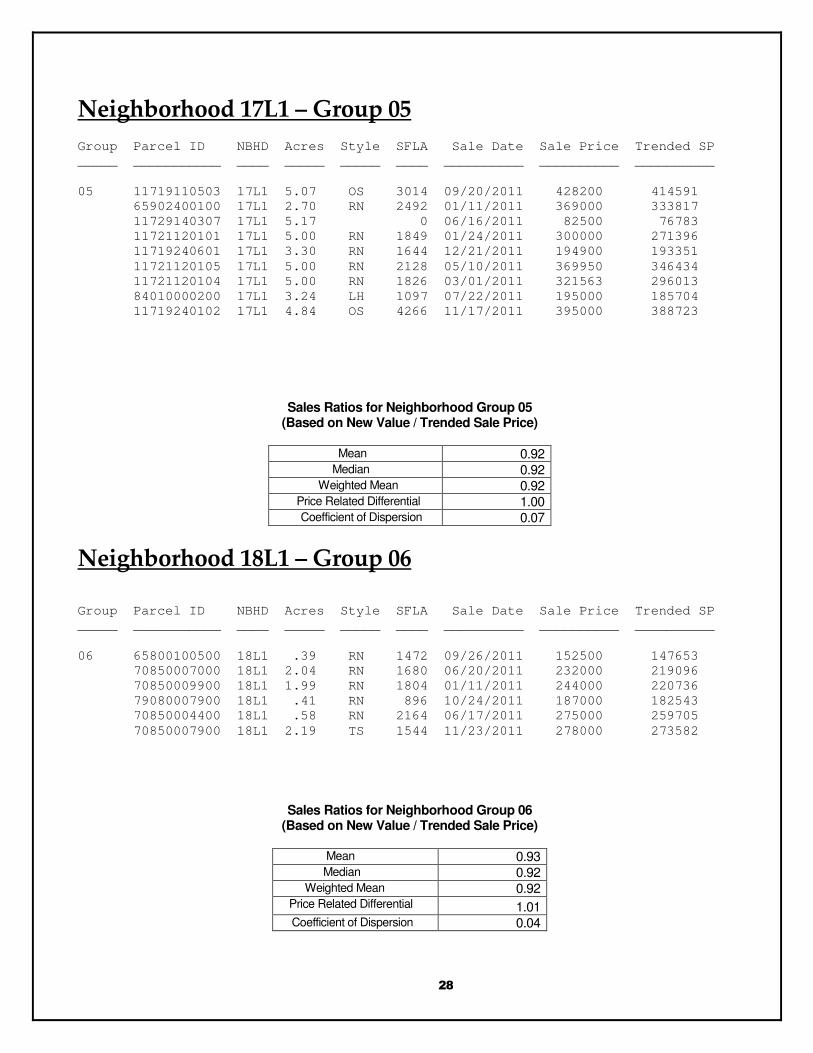
Neighborhood 17L1 – Group 05
Group Parcel ID NBHD Acres Style SFLA Sale Date Sale Price Trended SP
_____ ___________ ____ _____ _____ ____ __________ __________ __________
05 11719110503 17L1 5.07 OS 3014 09/20/2011 428200 414591
65902400100 17L1 2.70 RN 2492 01/11/2011 369000 333817
11729140307 17L1 5.17 0 06/16/2011 82500 76783
11721120101 17L1 5.00 RN 1849 01/24/2011 300000 271396
11719240601 17L1 3.30 RN 1644 12/21/2011 194900 193351
11721120105 17L1 5.00 RN 2128 05/10/2011 369950 346434
11721120104 17L1 5.00 RN 1826 03/01/2011 321563 296013
84010000200 17L1 3.24 LH 1097 07/22/2011 195000 185704
11719240102 17L1 4.84 OS 4266 11/17/2011 395000 388723
Sales Ratios for Neighborhood Group 05 (Based on New Value / Trended Sale Price)
Mean 0.92 Median 0.92
Weighted Mean 0.92 Price Related Differential 1.00 Coefficient of Dispersion 0.07
Neighborhood 18L1 – Group 06
Group Parcel ID NBHD Acres Style SFLA Sale Date Sale Price Trended SP
_____ ___________ ____ _____ _____ ____ __________ __________ __________
06 65800100500 18L1 .39 RN 1472 09/26/2011 152500 147653
70850007000 18L1 2.04 RN 1680 06/20/2011 232000 219096
70850009900 18L1 1.99 RN 1804 01/11/2011 244000 220736
79080007900 18L1 .41 RN 896 10/24/2011 187000 182543
70850004400 18L1 .58 RN 2164 06/17/2011 275000 259705
70850007900 18L1 2.19 TS 1544 11/23/2011 278000 273582
Sales Ratios for Neighborhood Group 06 (Based on New Value / Trended Sale Price)
Mean 0.93 Median 0.92
Weighted Mean 0.92 Price Related Differential 1.01 Coefficient of Dispersion 0.04
29
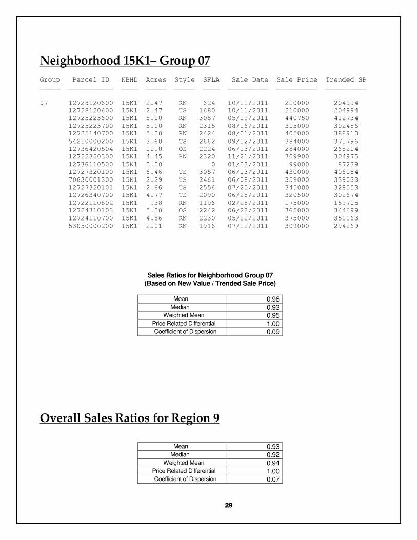
Neighborhood 15K1– Group 07
Group Parcel ID NBHD Acres Style SFLA Sale Date Sale Price Trended SP
_____ ___________ ____ _____ _____ ____ __________ __________ __________
07 12728120600 15K1 2.47 RN 624 10/11/2011 210000 204994
12728120600 15K1 2.47 TS 1680 10/11/2011 210000 204994
12725223600 15K1 5.00 RN 3087 05/19/2011 440750 412734
12725223700 15K1 5.00 RN 2315 08/16/2011 315000 302486
12725140700 15K1 5.00 RN 2424 08/01/2011 405000 388910
54210000200 15K1 3.60 TS 2662 09/12/2011 384000 371796
12736420504 15K1 10.0 OS 2224 06/13/2011 284000 268204
12722320300 15K1 4.45 RN 2320 11/21/2011 309900 304975
12736110500 15K1 5.00 0 01/03/2011 99000 87239
12727320100 15K1 6.46 TS 3057 06/13/2011 430000 406084
70630001300 15K1 2.29 TS 2461 06/08/2011 359000 339033
12727320101 15K1 2.66 TS 2556 07/20/2011 345000 328553
12726340700 15K1 4.77 TS 2090 06/28/2011 320500 302674
12722110802 15K1 .38 RN 1196 02/28/2011 175000 159705
12724310103 15K1 5.00 OS 2242 06/23/2011 365000 344699
12724110700 15K1 4.86 RN 2230 05/22/2011 375000 351163
53050000200 15K1 2.01 RN 1916 07/12/2011 309000 294269
Sales Ratios for Neighborhood Group 07 (Based on New Value / Trended Sale Price)
Mean 0.96 Median 0.93
Weighted Mean 0.95 Price Related Differential 1.00 Coefficient of Dispersion 0.09
Overall Sales Ratios for Region 9
Mean 0.93 Median 0.92
Weighted Mean 0.94 Price Related Differential 1.00 Coefficient of Dispersion 0.07

30
Multiple Regression Analysis Assumptions
Complete and Accurate Data:
• Data definitions and standards have been developed to ensure our data is as complete and accurate as possible.
• A procedure has been established to ensure sales are properly verified. • Annual training is conducted to remind appraisers of the standard that have been developed.
Representativeness:
• It is assumed that the sale sample adequately represents variables in the model. • Violation of this assumption may affect the accuracy of the model in predicting the value of properties that are
under-represented. For example, if there are no sales of “Excellent” view, the model would make no distinction from the typical “Average” view and an “Excellent” view. Using scalar or linearized variables in the model has mitigated this potential problem.
Linearity:
• It is assumed that the marginal contribution of a variable is constant over the range of values for the variable. Each additional unit of size or quantity adds equally to the value.
• The assumption is violated when economies of scale or other non-linear relationships are present. • Developing a multiplicative land model has helped to create linear relationships between the dependent variable
and independent variables. • For example, using the natural logarithm of the lot size (acres) addresses the decreasing marginal utility of
adding additional units of land. See example below.
Total Value
0
20000
40000
60000
80000
100000
120000
0 10 20 30 40 50
Acres
LN(Value)
10.400
10.600
10.800
11.000
11.200
11.400
11.600
0.000 1.000 2.000 3.000 4.000
LN(Acres)
Additivity:
• It is assumed that the marginal contribution of one independent variable is not affected by the changes in other variables.
• The assumption is violated when one impendent variable interacts with another. • This assumption generally does not hold for land models
o Land characteristics are often interactive. For example, the adjustment for view may be influenced by the size or topography of the land parcel.
• A multiplicative model helps to address this issue but converting the format to log-linear terms. No Correlation between Independent Variables:
• It is assumed that there is no correlation between independent variables. • This assumption is addressed by reviewing the correlation matrix and by either eliminating one of the correlated
variables or combining the highly correlated variables.
31
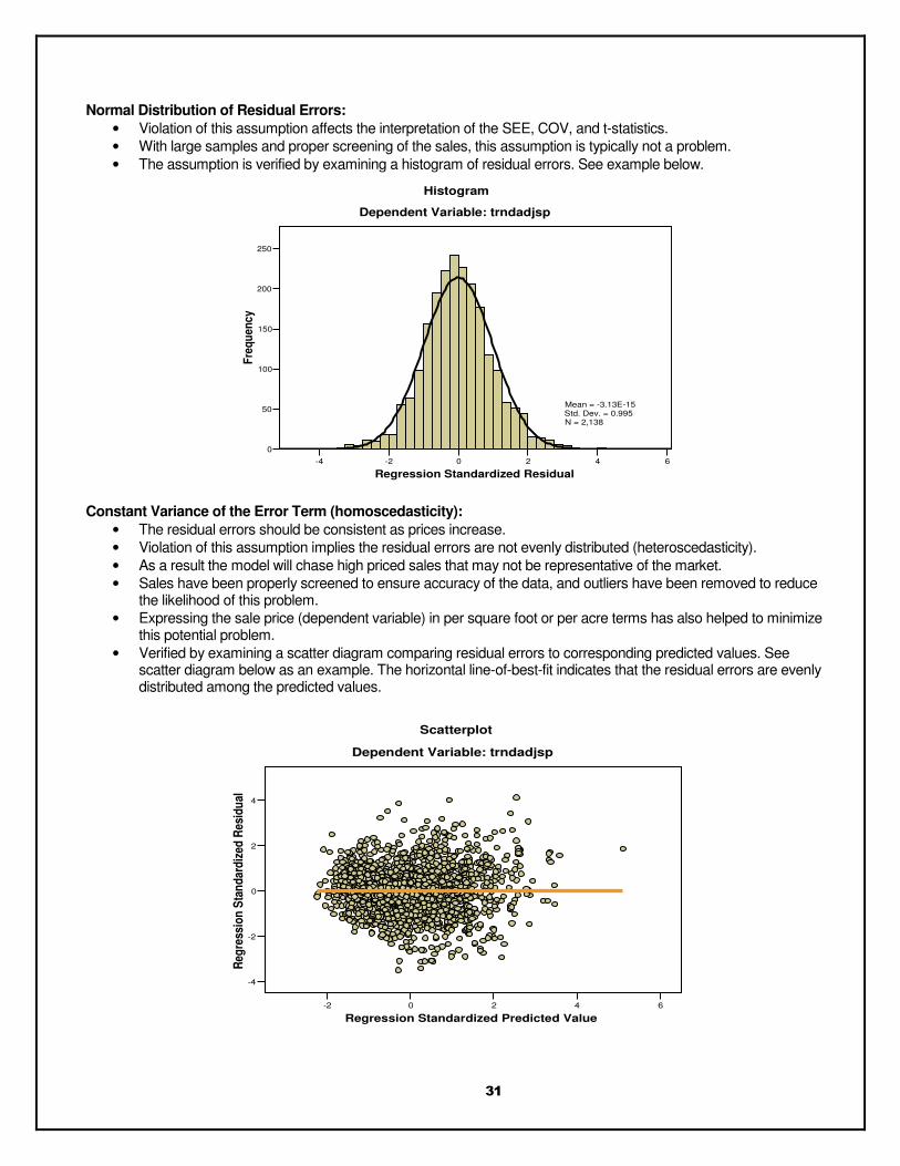
Normal Distribution of Residual Errors:
• Violation of this assumption affects the interpretation of the SEE, COV, and t-statistics. • With large samples and proper screening of the sales, this assumption is typically not a problem. • The assumption is verified by examining a histogram of residual errors. See example below.
-4 -2 0 2 4 6
Regression Standardized Residual
0
50
100
150
200
250F
req
ue
nc
y
Mean = -3.13E-15Std. Dev. = 0.995N = 2,138
Dependent Variable: trndadjsp
Histogram
Constant Variance of the Error Term (homoscedasticity):
• The residual errors should be consistent as prices increase. • Violation of this assumption implies the residual errors are not evenly distributed (heteroscedasticity). • As a result the model will chase high priced sales that may not be representative of the market. • Sales have been properly screened to ensure accuracy of the data, and outliers have been removed to reduce
the likelihood of this problem. • Expressing the sale price (dependent variable) in per square foot or per acre terms has also helped to minimize
this potential problem. • Verified by examining a scatter diagram comparing residual errors to corresponding predicted values. See
scatter diagram below as an example. The horizontal line-of-best-fit indicates that the residual errors are evenly distributed among the predicted values.
-2 0 2 4 6
Regression Standardized Predicted Value
-4
-2
0
2
4
Reg
ress
ion
Sta
nd
ard
ized
Res
idu
al
Dependent Variable: trndadjsp
Scatterplot