residual momentum - repub, erasmus university … momentum, on the other hand, is nearly neutral to...
TRANSCRIPT

�������� ����� ��
Residual Momentum
David Blitz, Joop Huij, Martin Martens
PII: S0927-5398(11)00004-1DOI: doi: 10.1016/j.jempfin.2011.01.003Reference: EMPFIN 538
To appear in: Journal of Empirical Finance
Received date: 5 October 2009Revised date: 10 December 2010Accepted date: 11 January 2011
Please cite this article as: Blitz, David, Huij, Joop, Martens, Martin, Residual Momen-tum, Journal of Empirical Finance (2011), doi: 10.1016/j.jempfin.2011.01.003
This is a PDF file of an unedited manuscript that has been accepted for publication.As a service to our customers we are providing this early version of the manuscript.The manuscript will undergo copyediting, typesetting, and review of the resulting proofbefore it is published in its final form. Please note that during the production processerrors may be discovered which could affect the content, and all legal disclaimers thatapply to the journal pertain.

ACC
EPTE
D M
ANU
SCR
IPT
ACCEPTED MANUSCRIPT
1
Residual Momentum
David Blitz, Joop Huij and Martin Martens*
Abstract
Conventional momentum strategies exhibit substantial time-varying exposures to
the Fama and French factors. We show that these exposures can be reduced by
ranking stocks on residual stock returns instead of total returns. As a
consequence, residual momentum earns risk-adjusted profits that are about twice
as large as those associated with total return momentum; is more consistent over
time; and less concentrated in the extremes of the cross-section of stocks. Our
results are inconsistent with the notion that the momentum phenomenon can be
attributed to a priced risk factor or market microstructure effects.
JEL Classification: G11, G12, G14
Keywords: momentum, time-varying risk, stock-specific returns, residual returns
* Blitz is at Robeco Quantitative Strategies, Huij is at Rotterdam School of Management and Robeco Quantitative Strategies and Martens is at Erasmus University Rotterdam and Robeco Quantitative Strategies. Email addresses are: [email protected]; [email protected]; and [email protected]. We are grateful for the comments of the referee and the editor, Chrisitan Wolff. The usual disclaimer applies.

ACC
EPTE
D M
ANU
SCR
IPT
ACCEPTED MANUSCRIPT
2
Residual Momentum
Abstract
Conventional momentum strategies exhibit substantial time-varying exposures to
the Fama and French factors. We show that these exposures can be reduced by
ranking stocks on residual stock returns instead of total returns. As a
consequence, residual momentum earns risk-adjusted profits that are about twice
as large as those associated with total return momentum; is more consistent over
time; and less concentrated in the extremes of the cross-section of stocks. Our
results are inconsistent with the notion that the momentum phenomenon can be
attributed to a priced risk factor or market microstructure effects.
JEL Classification: G11, G12, G14
Keywords: momentum, time-varying risk, stock-specific returns, residual returns

ACC
EPTE
D M
ANU
SCR
IPT
ACCEPTED MANUSCRIPT
3
1. INTRODUCTION
Conventional momentum strategies, as described in the seminal work of
Jegadeesh and Titman (1993; 2001), are based on total stock returns. In this
study we investigate in detail a momentum strategy based on residual returns
estimated using the Fama and French three-factor model. One of our main
findings is that the Sharpe ratio of residual momentum is approximately double
that of total return momentum, mainly due to lower return variability. The reason
is related to the fact that momentum has substantial time-varying exposures to
the Fama and French factors, as illustrated by Grundy and Martin (2001).
Specifically, momentum loads positively (negatively) on systematic factors when
these factors have positive (negative) returns during the formation period of the
momentum strategy. As a consequence, a total return momentum strategy
experiences losses when the sign of factor returns over the holding period is
opposite to the sign over the formation period. By design, residual momentum
exhibits smaller time-varying factor exposures, which reduces the volatility of the
strategy.
Residual momentum does not only improve upon total return momentum
in terms of higher long-run average Sharpe ratios, but also in several other ways.
First, total return momentum strategies appear to have lost their profitability in the
most recent years. In fact, we find a return of -8.5 percent per annum over the
period January 2000 to December 2009. Residual momentum, on the other hand,
has remained profitable, generating a return of 4.7 percent per annum over the
same time period. To illustrate that the negative returns of total return momentum

ACC
EPTE
D M
ANU
SCR
IPT
ACCEPTED MANUSCRIPT
4
strategies can largely be attributed to their time-varying exposures to the Fama
and French factors we point at the large losses of momentum in the first half of
2009. The negative market returns in the credit crises of 2008 caused total return
momentum to be tilted towards the low-beta segment of the market in early 2009.
When the market recovered in the first quarter of 2009, total return momentum’s
negative market beta caused large losses. Because residual momentum was
less negatively exposed to the market, the strategy was less negatively affected.
Second, a variety of papers argue that momentum displays characteristics
that are often associated with priced risk factors. Chordia and Shivakumar
(2002), for example, argue that the profits of momentum strategies exhibit strong
variation across the business cycle. Over the period January 1930 to December
2009, total return momentum earns 14.7 percent per annum during expansions
and loses –8.7 percent during recessions. We show that these results can largely
be attributed to the strategy’s time-varying exposures to the Fama and French
factors. A total return momentum strategy is typically titled towards low-beta
stocks after the early stage of a recession, while market returns during the later
stage of a recession are, on average, highly positive. Because residual
momentum is nearly market-neutral by construction, the strategy delivers positive
returns not only during expansions, but also during recessions. In particular, the
return of residual momentum during recessions is a positive 5.6 percent per
annum.
Third, another risk-based explanation for momentum is that the strategy is
concentrated in the smallest firms in the cross-section, see for example

ACC
EPTE
D M
ANU
SCR
IPT
ACCEPTED MANUSCRIPT
5
Jegadeesh and Titman (1993). Residual momentum, on the other hand, is nearly
neutral to the Fama and French size factor, indicating that the success of
momentum strategies is not critically dependent on a structural tilt towards small-
caps. Moreover, because, unlike total return momentum, residual momentum is
not concentrated in small-cap stocks, trading costs are likely to have a smaller
impact on profitability of the strategy.
Finally, residual momentum is less prone to the tax-loss selling effect
compared to total return momentum. Fund managers tend to sell small-cap loser
stocks in December, causing a large positive return for a total return momentum
strategy during that month, followed by a large negative return in January [see,
e.g., Roll (1983), Griffiths and White (1993), and Ferris, D'Mello, and Hwang
(2001)]. Because residual momentum is closer to being size neutral than total
return momentum, this December/January effect is much less pronounced, as a
result of which the strategy earns more stable returns within a calendar year.
Our work extends the research by Grundy and Martin (2001) who show
that momentum has dynamic exposures to the Fama and French factors. The
authors find a significantly improved performance for a hypothetical strategy
which hedges these exposures by adding positions in zero-cost hedge portfolios
based on ex post estimates of factor exposures. However, when they evaluate a
feasible strategy which uses information that is available ex ante they only find a
marginal improvement in performance. The residual momentum strategy
described in this paper, on the other hand, succeeds in improving upon a total

ACC
EPTE
D M
ANU
SCR
IPT
ACCEPTED MANUSCRIPT
6
return momentum strategy without using any information or instruments that
would not have been available to investors in reality.
Our work also extends the research by Guitierrez and Pirinsky (2007), who
document that momentum’s long-term reversal in month 13 to 60 after portfolio
formation can be attributed to the strategy’s common-factor exposures. For a
momentum strategy based on residual stock returns the authors observe that
performance over the first year after formation is similar to that of total return
momentum, but, contrary to total return momentum, long-run performance does
not revert. This suggests that the difference between residual and total return
momentum is negligible in the first year after formation and only becomes
significant during subsequent years. However, we show that when risks are taken
into account the momentum strategies’ performances are in fact also different
during the first 12 months after portfolio formation. As discussed above, we find
that the risk-adjusted performance of residual momentum is double that of total
return momentum; more consistent over time; more consistent over the business
cycle; and less concentrated in the extremes of the cross-section.
Our findings are consistent with the gradual-information-diffusion
hypothesis that states that information diffuses only gradually across the
investment public and that investor under-reaction is more strongly pronounced
for firm-specific events than for common events [see, e.g., Barberis, Schleifer
and Vishny (1998), Daniel, Hirschleifer and Subrahmanyam (1998), Hong and
Stein (1999), Hong, Lim and Stein (2000) and Gutierrez and Pirinsky (2007)].
Moreover, our results present an even more serious challenge to the view that

ACC
EPTE
D M
ANU
SCR
IPT
ACCEPTED MANUSCRIPT
7
markets are weak-form efficient than the total return momentum results in the
literature.
Our findings also have implications for the practical implementation of
momentum trading strategies. Our results imply that momentum investors in
practice are more likely to achieve a superior risk-adjusted performance by
adopting a residual momentum strategy than by following a conventional total
return momentum strategy.
In what follows, Section 2 discusses our motivation to look at residual
momentum. Section 3 describes our data and construction of momentum
portfolios. Sections 4 and 5 document the results of our empirical analyses and
robustness tests, respectively. Finally Section 6 concludes.
2. RESIDUAL MOMENTUM VERSUS TOTAL RETURN MOMENTUM
A conventional momentum strategy first ranks stocks on their total return over the
preceding period and then buys the past winner stocks and sells the past loser
stocks. We argue that such a strategy implicitly places a bet on persistence in
common-factor returns, which will affect its risk and return characteristics. To
illustrate this, consider the following example. If the market premium was positive
during the formation period, a momentum strategy will typically be long in high-
beta stocks and short in low-beta stocks, as high-beta stocks tend to outperform
low-beta stocks when the market goes up. As a consequence, the net market
beta of the momentum strategy will be positive. Similarly, when stocks with a high
(low) book-to-market ratio performed relatively well during the formation period,

ACC
EPTE
D M
ANU
SCR
IPT
ACCEPTED MANUSCRIPT
8
the strategy will be tilted towards value (growth) stocks. The profitability of a
momentum strategy will be positively affected by these dynamic exposures in
case of persistence in factor returns, but negatively when factor returns revert. In
addition a substantial part of the risk of momentum returns will be caused by the
factor exposures. In fact we will show in Section 4.1 that roughly 50 percent of
the risks, but only 25 percent of the profits of a conventional momentum strategy
can be attributed to the time-varying exposures to the Fama and French factors.
We look at a momentum strategy based on residual returns and focus on
two main aspects of the strategy. First, we show that ranking stocks, not on their
total returns, but on their residual returns is a very effective approach to
neutralize the dynamic factor exposures of a momentum strategy. We find that
these exposures are roughly three to five times smaller than those of a total
return momentum strategy. Second, the return and risk characteristics of residual
momentum allow us to substantiate various claims made about the return and
risk characteristics of total return momentum.
Regarding the first point, we find that residual momentum has comparable
returns to total return momentum at only half the risk. With a Sharpe ratio varying
between 0.4 and 0.9 depending on the holding period residual momentum is a
real-time feasible strategy. Grundy and Martin (2003) reduce the exposures of
total return momentum by a hedging strategy that uses ex-post available
information. They find that this makes momentum strategies more profitable, but
when they evaluate a feasible strategy which uses information that is available ex

ACC
EPTE
D M
ANU
SCR
IPT
ACCEPTED MANUSCRIPT
9
ante they only find a marginal improvement in performance. They leave the
development of a real-time available hedging strategy for further research.
Regarding the second point, by comparing the risk and return
characteristics of residual momentum strategies with those of conventional total
return momentum strategies we can produce a number of convincing
explanations regarding earlier findings in the literature. These explanations are all
related to the time-varying exposures of total return momentum to the Fama and
French factors. For example, the time-varying exposures of total return
momentum caused to a large extent its poor performance in the past decade, see
Section 4.2. Also, the poor performance of total return momentum during
recessions reported by Chordia and Shivakumar (2002) can to a large extent be
attributed to the time-varying risk exposures as discussed in Section 4.3. Finally,
the poor performance of momentum in Januaries reported in Jegadeesh and
Titman (1993) is caused by momentum being short in small-cap loser stocks that
are aggressively sold in December but tend to recover in January, see Section
4.5.
3. DATA AND METHODOLOGY
Consistent with most of the momentum literature, we extract our data from the
CRSP database and consider all domestic, primary stocks listed on the New York
(NYSE), American (AMEX), and Nasdaq stock markets in our study. Closed-end
funds, Real Estate Investment Trusts (REITs), unit trusts, American Depository
Receipts (ADRs), and foreign stocks are excluded from the analysis. Our sample

ACC
EPTE
D M
ANU
SCR
IPT
ACCEPTED MANUSCRIPT
10
period covers the period January 1926 to December 2009. We exclude stocks
during the month(s) that their price is below $1 to reduce microstructure
concerns. Our data on common factors are from the webpage of French (2010).
Our analysis of momentum strategies follows the common approach in the
empirical literature [see, e.g., Jegadeesh and Titman (1993; 2001), Chan,
Jegadeesh, and Lakonishok, (1996), Rouwenhorst (1998; 1999), Griffin, Ji and
Martin (2003), Grundy and Martin (2003), Schwert (2003), and Gutierrez and
Pirinsky (2007)]. The methodology involves ex ante formation of portfolios based
on past returns, followed by ex post factor regressions of the resulting
(overlapping) portfolio returns on common risk factors.
We start by allocating stocks to mutually exclusive decile portfolios based
on their returns over the preceding 12 months excluding the most recent month
(henceforth denoted by 12-1M). Stocks are ranked on both total returns and
residual returns. The reason why we focus on the 12-1M formation period
throughout our main analyses is that this momentum definition is currently most
broadly used and readily available though the PR1YR factor of Carhart (1997)
and the WML factor from the webpage of French (2010).1 Residual returns are
estimated each month for all eligible stocks using the Fama and French three-
factor model:
(1) titititiiti HMLSMBRMRFr ,,3,2,1,
1 Month t-1 in the formation period of momentum strategies is typically skipped to disentangle the
intermediate-term momentum effect from the short-term reversal effect documented by Jegadeesh (1990) and Lehman (1990).

ACC
EPTE
D M
ANU
SCR
IPT
ACCEPTED MANUSCRIPT
11
where tir , is the return on stock i in month t in excess of the risk-free rate, tRMRF ,
tSMB and tHML are the excess returns on factor-mimicking portfolios for the
market, size and value in month t, respectively, i , i,1 , i,2 and i,3 are
parameters to be estimated, and ti , is the residual return of stock i in month t.
We estimate the regressions over 36-month rolling windows, i.e., over the period
from t-36 until t-1, so that we have a sufficient number of return observations to
obtain accurate estimates for stock exposures to the market, size and value. Only
stocks which have a complete return history over the 36-month rolling regression
window are included in our analysis.
With the momentum portfolios based on total return momentum, the top
(bottom) decile contains the 10 percent of stocks with the highest (lowest) 12-1M
total returns. With the portfolios based on residual momentum, the top (bottom)
decile contains the 10 percent of stocks with the highest (lowest) 12-1M residual
return standardized by its standard deviation over the same period. The reason
for standardizing the residual return is to obtain an improved measure, since the
raw residual return can be a noisy estimate. Guitierrez and Pirinsky (2007) also
standardize residual returns when they investigate the interaction between
idiosyncratic stock return variation and long-run reversals. They argue that
standardizing the residual return yields an improved measure of the extent to
which a given firm-specific return shock is actually news, opposed to noise,
thereby facilitating a better interpretation of the residual as firm-specific

ACC
EPTE
D M
ANU
SCR
IPT
ACCEPTED MANUSCRIPT
12
information.2 Note that we do not include the estimated alpha in the calculation of
residual momentum because the alpha serves as a general control for
misspecification in the model of expected stock returns. Moreover, over two-
thirds of the observations behind the estimated alpha are outside the 11-month
formation period which is relevant for residual momentum, as a result of which
the alpha may, to a large extent, reflect extreme return observations in month t-
36 to t-13. For example, if we would include the estimated alpha in the calculation
of residual momentum, stocks that had large positive (negative) returns over the
period t-36 to t-13, would rank low (high) on residual momentum. As such, the
resulting residual momentum strategy might not only reflect the intermediate-term
momentum effect, but also the long-term reversal effect.
Consistent with most of the literature, we assign equal weights to the
stocks in each decile. We form the deciles using monthly, quarterly, semi-
annually and yearly holding periods using the overlapping portfolios approach of
Jegadeesh and Titman (1993; 2001). With this approach, the strategies hold a
series of portfolios, in any given month, that are selected in the current month as
well as in the previous K-1 months, where K is the holding period.
Next, we consider the post-formation returns over the period January 1930
to December 2009 for the return differential between the top and bottom deciles.
We look at the momentum strategies’ returns, volatilities, Sharpe ratios and
2 We also test residual momentum strategies where the returns are not standardized. It seems
that standardizing returns indeed helps to obtain a slightly improved measure. For example, using one-month holding periods, the non-standardized residual momentum strategy yields a return of 11.88 percent per annum, a volatility of 13.28 percent, and a Sharpe ratio of 0.89. Compared to the results in Table 2 we observe that standardizing in particular helps to further reduce the risk of the strategy.

ACC
EPTE
D M
ANU
SCR
IPT
ACCEPTED MANUSCRIPT
13
alphas relative to the Fama and French factors. To estimate alphas, we employ a
conditional framework in the spirit of Grundy and Martin (2001) to account for the
dynamic factor exposures of momentum strategies:
(2) tititi
titititiiti
UPHMLUPSMB
UPRMRFHMLSMBRMRFr
,,3,2
,4,3,2,1,
__
_
where tUPRMRF _ , tUPSMB_ and tUPHML _ are interaction variables that are
equal to the excess returns on factor-mimicking portfolios for the market, size and
value in month t, respectively, when the premiums on the factors are positive
over month t-12 to t-2, and zero otherwise.
In later robustness checks (see Section 5), we show that residual
momentum behaves consistently when we use the broad (J,K) momentum
strategies of Jegadeesh and Titman (1993); when we restrict our sample to large
cap stocks; when we use alternative specifications of common factors; when we
use different lengths for the rolling window we use to estimate the betas to the
factor-mimicking portfolios for the market, size and value in Equation (1); and
when we consider the post-1960 period of our sample.
4. EMPIRICAL RESULTS
This section contains an extensive comparison of the empirical characteristics of
residual and total return momentum strategies.

ACC
EPTE
D M
ANU
SCR
IPT
ACCEPTED MANUSCRIPT
14
4.1 Main results
We start our empirical investigation by comparing and distinguishing between the
performances of total return momentum and residual momentum. The main
testable prediction which we explore is that residual momentum has significantly
lower exposures to common factors than total return momentum, resulting in a
significantly lower volatility of the strategy. At the same time we investigate which
portion of the profitability of total return momentum can be attributed to dynamic
factor exposures and how profitability is affected by following a residual
momentum strategy instead.
To go to the heart of the issue, we examine if there is persistence in
common factor returns. As we explained previously, persistence in common
factor returns can potentially contribute positively to momentum’s profitability. We
test for persistence by measuring the frequency with which the signs of the factor
returns are the same during the formation period and the holding period.
Consistent with the definition of our momentum portfolios, we use 12-month
formation periods excluding the most recent month. We use alternative holding
periods of one month, one quarter, six months and one year. The results are in
Table 1.
[INSERT TABLE 1 ABOUT HERE]
Under the null hypothesis of no persistence in factor returns, the
frequencies in Table 1 should equal 50 percent. However, our empirical results
show that the frequencies tend to be between 54 and 61 percent, which indicates
that there is at least some amount of persistence in common factor returns. The

ACC
EPTE
D M
ANU
SCR
IPT
ACCEPTED MANUSCRIPT
15
t-statistics resulting from differences-in-means tests indicate that the observed
frequencies are significantly different from 50 percent.3
Given the evidence of persistence in common factor returns we may
expect the dynamic factor exposures of a total return momentum strategy to
contribute positively to profitability. However, the question remains how large this
contribution to performance is; how much risk is involved with these exposures;
and what happens when we attempt to neutralize these dynamic exposures.
We therefore continue by decomposing the risks and profits of total return
momentum and residual momentum into a component due to persistence in
common factor returns and a component due to persistence in residual returns
using the conditional Fama and French model in Equation (2). The results in
Panel A of Table 2 show that total return momentum exhibits strong dynamic
exposures to the Fama and French factors. The exposures to the market, size
and value factors are both economically and statistically significant. Momentum
loads negatively on factors after negative returns, and positively after positive
returns. For example, total return momentum’s market beta is -0.34 after negative
market returns in the formation period for one-month holding periods, and 0.34 (=
-0.34 + 0.68) after positive market returns. The results are independent of the
length of the holding period. The adjusted R-squared values of the regressions
3 Two effects may be driving the persistence in factor returns: positive autocorrelation in factor
returns and positive factor premiums (or, more specifically, a larger than 50 percent probability that factor returns are positive). To illustrate the latter point, suppose that factor returns exhibit zero autocorrelation but have a 60 percent probability of being positive. In that case the probability of two subsequent returns having the same sign is 52 percent (= 0.60 x 0.60 + 0.40 x 0.40). Unreported results indicate that, indeed, both effects contribute to the persistence reported in Table 1. However, for the purposes of this paper our main concern is whether there is persistence, while the mechanism behind this is less relevant. We therefore do not further investigate this issue.

ACC
EPTE
D M
ANU
SCR
IPT
ACCEPTED MANUSCRIPT
16
indicate that up to 48 percent of the variance of total return momentum can be
explained by dynamic factor exposures. These findings underline the importance
of taking into account dynamic risk exposures when evaluating the risks and
profits of momentum strategies.4
[INSERT TABLE 2 ABOUT HERE]
The results in Panel B of Table 2 indicate that residual momentum, on the
other hand, exhibits smaller factor exposures. More specifically, the conditional
betas to the Fama and French factors of residual momentum are roughly three to
five times smaller than those of total return momentum. For the one-month
holding period, for example, the market beta after market declines during the
formation period is –0.34 for total return momentum, versus –0.12 for residual
momentum. The explanatory power of the regressions is also substantially lower
for residual momentum with the regression R-squared values ranging from 13 to
17 percent, compared to 34 to 48 percent for total return momentum. We can
thus conclude that ranking stocks by their residual return turns out to be an
effective approach to reduce the dynamic factor exposures of conventional
momentum strategies.
To further investigate the impact of neutralizing momentum’s dynamic
factor exposures on portfolio risk, we evaluate the volatilities of total return
momentum and residual momentum. We find that the volatility of residual
momentum is only about half that of total return momentum. For example, using
one-month holding periods, total return momentum has an annualized volatility of
4 When we evaluate the performance of total return momentum using the unconditional Fama-
French model in Equation (1), the adjusted R-squared values of the regressions indicate that only 10 to 17 percent of the variance of the momentum strategy can be explained by factor exposures.

ACC
EPTE
D M
ANU
SCR
IPT
ACCEPTED MANUSCRIPT
17
22.70 percent, versus 12.49 percent for residual momentum. Hence, ranking
stocks by their residual return substantially reduces the risk of a momentum
strategy.
We next turn to investigating the impact of neutralizing momentum’s
dynamic factor exposures on the strategy’s profitability. As expected, we can
conclude that the dynamic style exposures of total return momentum are
contributing positively to profitability, as the alphas of the total return momentum
strategies are roughly 25 percent lower than their raw returns. For example,
using one-month holding periods, the return of total return momentum is 10.26
percent per annum, while the alpha in this case is 7.98 percent. Importantly, the
portion of the risk of total return momentum that can be attributed to these
exposures is substantially larger (i.e., the adjusted R-squared values from the
regressions indicate that this portion is about 50 percent). Therefore one might
expect residual momentum to have a lower return, but a higher Sharpe ratio than
total return momentum.
One of our key findings, however, is that ranking stocks on their residual
return does not come at the expense of the profitability of the strategy. Both the
return and the alpha of residual momentum are in fact higher than those of total
return momentum. For example, Table 2 shows that, using one-month holding
periods, the return of residual momentum is about one percent higher than that of
total return momentum, while the alpha is even 2.9 percent higher. In order to
understand this result, we first note that, compared to total return momentum,
residual momentum has less weight in stocks with large exposures to common

ACC
EPTE
D M
ANU
SCR
IPT
ACCEPTED MANUSCRIPT
18
factors, but more weight in stocks with high residual returns. Our results imply
that the loss in profitability which results from the first effect is more than
compensated for by a gain in profitability which is associated with the second
effect. Hence, despite our finding that factor returns tend to persist to a certain
degree, the dynamic factor exposures of total return momentum strategies are
not only suboptimal from a risk point of view, but also from a return perspective.
Because a residual momentum strategy yields profits similar to a total
return momentum strategy, but with a volatility that is roughly 45 percent lower,
the Sharpe ratio of residual momentum is approximately double that of total
return momentum. Therefore, when we use the Sharpe ratio as the criterion to
evaluate the magnitude of anomalies, this implies that momentum, which is
already one of the most significant anomalies in empirical finance, is twice as
large an anomaly if stocks are ranked on their residual return instead of their total
return.5 Our empirical results are consistent with the body of literature that
attempts to explain the momentum anomaly by behavioural biases of investors
[see, e.g., Barberis, Schleifer and Vishny (1998), Daniel, Hirschleifer and
Subrahmanyam (1998), and Hong and Stein (1999)]. In particular, our finding that
the largest portion of the profits of total return momentum can be attributed to
exposures to idiosyncratic factors is supportive of the gradual-formation-diffusion
hypothesis of Hong and Stein (1999) that predicts that firm-specific information
diffuses only gradually across the investment public.
5 Following the work of Jegadeesh and Titman (1993), momentum has been investigated by other
authors in the United States before 1960s; in areas outside the United States; and subsequent to the period after the publication of their results [see, e.g., Rouwenhorst (1998, 1999), Jegadeesh and Titman (2001), Griffin, Ji and Martin (2003), and Schwert (2003)].
ACC
EPTE
D M
ANU
SCR
IPT
ACCEPTED MANUSCRIPT
19
Another important implication of our findings is that residual momentum is
a substantially longer-lived phenomenon than total return momentum. While the
alpha of total return momentum decreases to an economically and statistically
insignificant figure of 0.56 percent using a 12-month holding period, residual
momentum still generates significant risk-adjusted returns of over four percent
per annum at this horizon. This finding is inconsistent with the view that
momentum profits can only be captured using a short holding period, but in line
with the recent findings of Gutierrez and Pirinsky (2007), who focus on the long-
term performance of residual versus total return momentum strategies in their
study. They find that, whereas total return momentum profits revert at horizons
beyond one year, residual momentum continues to generate positive returns.
4.2 Performance differences over time
Proceeding further, we investigate how the performance differential between the
two momentum strategies evolves over time. Are there, for example, specific time
periods in which reversals in factor returns hurt the performance of total return
momentum because of its exposures to the Fama and French factors? To
investigate this issue, we first examine the cumulative performances (Figure 1)
and drawdowns (Figure 2) of total return momentum and residual momentum
using one-month holding periods. The drawdown at any given moment is
calculated by comparing the cumulative return at that point in time to the all-time
high cumulative return which was achieved up to that point in time. By definition,

ACC
EPTE
D M
ANU
SCR
IPT
ACCEPTED MANUSCRIPT
20
therefore, the drawdown is zero percent at best, in case the strategy is at an all-
time high, and negative otherwise.
[INSERT FIGURES 1 AND 2 ABOUT HERE]
Figures 1 and 2 show that residual momentum generates more consistent
returns than total return momentum. For example, in our sample period total
return momentum suffers from a maximum drawdown magnitude of 85 percent
negative during the early 1930s, from which it takes over 19 years to recover.
Residual momentum also suffers its worst drawdown during this period, but with
a magnitude and length less than half as severe as for total return momentum.
The second worst drawdown for total return momentum and residual momentum
occurs during the most recent decade. During the post-2000 period total return
momentum suffers a drawdown exceeding 80 percent, while residual momentum
limits the drawdown in this period to about 40 percent.
To investigate the impact of the large drawdowns on momentum profits
over time we list the performances of total return momentum and residual
momentum per decade in Table 3. For comparison, the table also shows the
returns per decade on the market, size and value factors and the risk-free rate.
[INSERT TABLE 3 ABOUT HERE]
The results in Table 3 show that total return momentum does not earn a
premium over the decades in which it suffers its two largest drawdowns; the
1930s and the post-2000 period. Moreover, the momentum premium during the
1970s is only marginally significant from a statistical point of view. Residual
momentum, on the other hand, delivers annualized returns of at least four-and-a-

ACC
EPTE
D M
ANU
SCR
IPT
ACCEPTED MANUSCRIPT
21
half percent per annum during each decade in our sample, and, except for the
most recent decade, the residual momentum premium is statistically significant
for all decades in our sample. Compared to the returns on the other factors in the
Fama and French three-factor model, both momentum strategies have
economically large and statistically significant premiums. For example, the
premium on the market factor is only statistically significant during two out of
eight decades; and the premium on the size and value factors is only statistically
significant during one or two decades in our sample.
To better understand how the differences in exposures to the Fama and
French factors between total return momentum and residual momentum cause
the large return differences in the 1930s and the post-2000 period, we take a
detailed look at the returns of both momentum strategies during the years 2009
and 1932, when the return differences between the momentum strategies are the
largest. The returns over these years of the momentum strategies and the market
are shown in Figure 3.
[INSERT FIGURE 3 ABOUT HERE]
In both years a strong market reversal occurred after a severe economic
recession. For example, during the credit crisis in 2008 the return on the market
factor was -39 percent. This negative return caused total return momentum to be
tilted towards the low-beta segment of the market early 2009. When the market
recovered in 2009 with returns of 9, 11, and 7 percent over the months March,
April, and May, respectively, total return momentum’s negative market beta
caused a streak of large losses. Because residual momentum was less

ACC
EPTE
D M
ANU
SCR
IPT
ACCEPTED MANUSCRIPT
22
negatively exposed to the market, the strategy was less negatively affected.
While the ex post market beta over 2009 was -0.9 for total return momentum, this
figure was -0.3 for residual momentum.6 We see a very similar pattern in the year
1932. Following a market return of -49 percent in 1931, a recovery followed with
large positive returns of 34 and 37 percent in July and August 1932, respectively.
Again total return momentum was tilted towards the low-beta segment of the
market at the end of 1931 and suffered large losses during the recovery with an
ex post market beta of -1.1 over 1932. At -0.3, the market beta of residual
momentum was again substantially lower, causing smaller losses. We conclude
that although long-term average returns may be similar, the differences in
exposures to the Fama and French factors between total return momentum and
residual momentum may cause large return differences between the strategies in
the short run.
4.3 Business cycle effects
Having established that the largest return differences between total return
momentum and residual momentum occur when the factor returns in the
investment period are opposite to those during the formation period, we continue
our analysis with investigating the performance of total return momentum and
residual momentum over the business cycle. Chordia and Shivakumar (2002)
report that total return momentum performs poorly during contractions as defined
by the NBER. Because of this characteristic, momentum returns are often
associated with a priced risk factor. We argue that the poor performance of total
6 The reported market betas are estimated using the regression model in Equation (1).

ACC
EPTE
D M
ANU
SCR
IPT
ACCEPTED MANUSCRIPT
23
return momentum during economic contractions can be attributed to the stylized
fact that the largest market reversals tend to take place during recessionary
periods. For example, over our sample period from January 1930 to December
2009, the average return on the market factor is -22.9 percent per annum in the
early phase of economic recessions as defined by the NBER business cycle
indicator, while its average return is 10.9 percent in the late phase.7 As we have
seen in our previous analysis, we expect total return momentum to tilt towards
the low-beta segment of the market after early recessions, which causes large
underperformance when the market recovers during the late recessionary
phases. Because residual momentum exhibits significantly smaller exposures to
the Fama and French factors, we expect the strategy to be less affected by
business cycle effects. To investigate this issue, we evaluate the returns of total
return and residual momentum strategies with one-month holding periods during
NBER expansion or contraction phases.
[INSERT TABLE 4 ABOUT HERE]
The results in Table 4 indicate that total return momentum has a high
average performance during expansionary periods, at 14.70 percent per annum.
In contrast, the performance is -8.73 percent per annum during recessionary
periods. We attribute this negative performance to the large market reversals that
typically take place during economic contractions. Panel B of Table 4 which
shows the results during the early and late stages of expansions and recessions
confirms that the losses of total return momentum during recessions are indeed
7 We define the early and late phase of expansions and recessions by splitting the period exactly
halfway.

ACC
EPTE
D M
ANU
SCR
IPT
ACCEPTED MANUSCRIPT
24
concentrated in the second half of recessions, when the market tends to revert.
When we consider the performance of residual momentum, shown in the final
column of Table 4, we see that the performance of residual momentum is quite
stable over the business cycle. During recessions it still averages returns above
five-and-a-half percent per annum, and even during the second half of recessions
it manages to avoid a negative return. By design residual momentum has less
dynamic exposures to the factor returns and hence it is not susceptible to losses
when factor returns revert. When we calculate market betas of both momentum
strategies during late recessions, we find a beta of -0.74 for total return
momentum and a beta of -0.24 for residual momentum. These results are
consistent with our notion that total return momentum strategies tend to tilt
towards the low-beta segment of the market during early recessionary periods
and that this effect is less pronounced for residual momentum. Overall, our
results indicate that residual momentum produces consistent alpha in all
economic environments, which makes it more difficult to attribute this anomaly to
a priced risk factor.
4.4 Small-cap stock exposures, distress risk and trading costs
Apart from the fact that total return momentum tends to be exposed to common
factors with positive one-year returns, the strategy is also systematically
concentrated in the small-cap segment of the market. Jegadeesh and Titman
(1993), for example, show that the top and bottom deciles of stocks ranked on
total return on average contain high-beta and small-cap stocks. In this subsection

ACC
EPTE
D M
ANU
SCR
IPT
ACCEPTED MANUSCRIPT
25
we illustrate the corresponding characteristics of residual momentum. In Table 5
we therefore report the average pre- and post-ranking returns and volatilities, as
well as the unconditional ex post exposures to the market, size and value factors,
for each decile portfolio and for the D10-D1 hedge portfolio.
[INSERT TABLE 5 ABOUT HERE]
As expected, we observe that total return momentum has a higher
dispersion in pre-ranking returns and volatility. Consistent with the findings of
Jegadeesh and Titman (1993), we also find that the decile 1 and 10 portfolios
have a higher market beta and a lower market cap than the other deciles.
Moreover, it appears that the extreme portfolios exhibit increased levels of firm-
specific risk. Campbell and Taksler (2003) show that these characteristics are
positively related to bond yields. As such, our findings are consistent with the
notion of Agarwal and Taffler (2008), and Avramov et al. (2007) that momentum
trading strategies are concentrated in the highest credit-risk firms that are more
likely to suffer financial distress.
The corresponding characteristics of decile portfolios of stocks sorted on
their residual momentum appear to be quite different. We first note that ex post
the average returns of the residual momentum deciles increase more
monotonically than those of total return momentum, also resulting in the slightly
higher spread of 11.20 percent between deciles 10 and 1, compared to 10.26
percent of total return momentum. Furthermore, residual momentum only has
minor differences in market betas and size exposures across all deciles. Hence,
residual momentum does not appear to be tilted towards a specific market

ACC
EPTE
D M
ANU
SCR
IPT
ACCEPTED MANUSCRIPT
26
segment of the equity market such as small-cap stocks with elevated levels of
firm-specific risk.
Another critical view on the momentum anomaly is that its profits are
difficult to capture because the strategy is concentrated in stocks that involve
high trading costs [see, e.g., Lesmond, Schill and Zhou (2004), and Korajczyk
and Sadka (2006)]. Keim and Madhavan (1997) and De Groot, Huij, and Zhou
(2011) report that market capitalization and stock volatility are important
determinants in explaining stock trading costs. For example, Keim and Madhavan
(1997) report that the trading costs of the bottom quintile of stocks ranked on
market capitalization can be more than ten times larger than the costs of the top
quintile of stocks. Because residual momentum is neutral to both factors, it
follows that trading costs are likely to have a smaller impact on the profitability of
residual momentum than total return momentum.
4.5 Calendar month effects
Finally, we investigate the performances of total return momentum and residual
momentum per calendar month. Several authors document strong seasonal
patterns in momentum returns. For example, Jegadeesh and Titman (1993;
2001) and Grinblatt and Moskowitz (2004) find a January effect for the total
return momentum strategy. In particular, average returns in January are found to
be negative. The cited reason is the tax-loss selling effect. Fund managers tend
to sell small-cap loser stocks in December, resulting in downward price pressure
in that month, which is followed by a correction in January. Because a total return

ACC
EPTE
D M
ANU
SCR
IPT
ACCEPTED MANUSCRIPT
27
momentum strategy is typically short in small-cap loser stocks, this effect causes
a large positive return for the strategy in December followed by a large negative
return in January. We refer to Roll (1983), Griffiths and White (1993), and Ferris,
D'Mello, and Hwang (2001) for a detailed documentation of this effect.
Because residual momentum is less concentrated in small-cap stocks
compared to total return momentum, we expect the January effect to have a
smaller impact on the strategy’s performance. To investigate this issue in more
detail, we examine the average monthly returns during each calendar month for
the total return momentum versus the residual momentum strategies.
[INSERT TABLE 6 ABOUT HERE]
The results in Panel A of Table 6 confirm the strong negative performance
of total return momentum in Januaries, with an average return of –2.60 percent.
Residual momentum, on the other hand, earns an average (non-significant)
return of –0.32 percent in Januaries, as shown in Panel B of Table 6.
Our results illustrate another notable seasonality in momentum returns.
We observe that most of the profits of total return momentum are generated in a
handful of months during the years. For example, the t-statistics of the strategy’s
returns exceed plus two only in three out of 12 months. By contrast, residual
momentum returns have t-statistics larger than plus two in eight out of 12
months. We thus conclude that residual momentum is also more robust than total
return momentum during the calendar year.
5. ROBUSTNESS CHECKS AND FOLLOW-UP EMPIRICAL TESTS

ACC
EPTE
D M
ANU
SCR
IPT
ACCEPTED MANUSCRIPT
28
In this final section we perform a range of tests to examine the robustness of our
results to various choices we made with respect to the design of our research.
5.1 (J,K) momentum strategies
To start with, we analyze the sensitivity of our results to our definition of
momentum, which is based on a 12-month formation period excluding the most
recent month. As mentioned before, we use this definition for our main analyses
because this definition of momentum is currently most broadly used. Some
researchers have used alternative momentum definitions though. To investigate if
the improvement of residual momentum over total return momentum is also
observed for alternative momentum definitions, we compare the risks and returns
of both strategies for the broad (J,K) momentum definitions of Jegadeesh and
Titman (1993). With these definitions, stock portfolios are formed based on J-
month lagged returns and held for K months, where J = {3,9,6,12} and K =
{3,9,6,12}. As in our previous analyses, we consider top-minus-bottom decile
returns using overlapping portfolios. For each (J,K) combination we compare
average returns, volatilities, and Sharpe ratios. If our residual momentum
approach is indeed successful in removing momentum’s time-varying exposures
to the Fama and French factors, we should observe that the volatilities of the
residual momentum strategies are consistently lower than those of the total
return momentum strategies.
[INSERT TABLE 7 ABOUT HERE]

ACC
EPTE
D M
ANU
SCR
IPT
ACCEPTED MANUSCRIPT
29
The results are reported in Table 7. The (J,K) momentum strategies exhibit
performance patterns that are very similar to what has been documented in the
literature. For short formation periods with J=3, we observe negative momentum
profits because of the short-term reversal effect [see, e.g., Jegadeesh (1990) and
Lehman (1990)]. In general returns for total return momentum are lower than in
Panel A of Table 2, where the skip month avoids the negative returns in the first
month after formation. The key take-away from Table 7 is that our residual
momentum approach yields higher Sharpe ratios than total return momentum
because of consistently lower volatility, independent of the parameters used to
define a momentum strategy. Even with the parameter combination which results
in the smallest improvement, residual momentum earns risk-adjusted profits that
are three times as large as those associated with total return momentum: with
J=6 and K=9 total return momentum earns a Sharpe ratio of 0.23, while residual
momentum earns a Sharpe ratio of 0.62. The difference here is even larger than
in Table 2 because residual momentum also has smaller losses in the skip month
than total return momentum and hence higher average returns.
Another momentum definition that is sometimes used employs a six-month
formation period where one month is skipped for the holding period [see, e.g.
Grundy and Martin (2001), and Gutierrez and Pirinsky (2007)]. We also compare
total return momentum to residual momentum using this definition. For total
return momentum we find a return of 5.17 percent for the top-minus-bottom
decile portfolio, a volatility of 23.22 percent, and a Sharpe ratio of 0.22. For
residual momentum we find a return of 6.10 percent, a volatility of 12.02 percent,

ACC
EPTE
D M
ANU
SCR
IPT
ACCEPTED MANUSCRIPT
30
and a Sharpe ratio of 0.51. These results corroborate our previous finding that
residual momentum earn higher risk-adjusted profits than total return momentum
because its volatility is roughly half. We conclude that our results are robust to
our choice of momentum definition.
5.2 Using strictly large cap stocks
Continuing our robustness checks, we address the concern that most of the
performance differential between total return and residual momentum might
come from the small-cap stocks in our sample. We therefore investigate if results
remain similar when the universe of stocks is restricted to large-cap stocks only.
In particular, we repeat the analysis on the 10 percent of stocks within our base-
case sample with, at each point in time, the largest market capitalizations. The
results are shown in Table 8.
[INSERT TABLE 8 ABOUT HERE]
The results based on our sample of large-cap stocks are not materially different
from our main results in Table 2. The most notable difference is that the portion
of the variability in the returns of total return momentum that can be attributed to
the Fama and French factors is somewhat lower. While the adjusted R-squared
values of our regressions in Panel A of Table 2 vary between 34 and 48 percent,
the corresponding figures in Table 8 vary between 31 and 33 percent. Also, the
time-varying exposures of the total return momentum strategies to the SMB
factor are smaller for our large-cap stock sample. In Panel A of Table 2 estimates
range between -0.62 and -0.82 for SMB and between 0.58 and 1.01 for

ACC
EPTE
D M
ANU
SCR
IPT
ACCEPTED MANUSCRIPT
31
SMB_UP, whereas these figures range between -0.25 and -0.39, and 0.40 and
0.72, respectively, for our sample of large-caps in Table 8. These results are not
surprising given the fact that our sample of large-cap stocks is, by definition,
more homogeneous in terms of market capitalization. Nonetheless, the time-
varying exposures to RMRF and HML remain substantial for total return
momentum strategies. Hedging out these exposures using our residual
momentum approach significantly improves the risk-adjusted performance of the
strategies for all holding periods. For example, total return momentum for large
cap stocks using one-month holding periods earns a Sharpe ratio of 0.36
compared to 0.60 for residual momentum. Hence our main conclusions remain
nearly unchanged when we restrict our sample to a universe of large cap stocks.
5.3 Industry effects
The next issue we investigate is related to the findings of several authors that the
Fama and French factors do not fully suffice to describe the returns on industry
portfolios [see, e.g., Fama and French (1997)]. While sorting stocks on their
residual return relative to the Fama and French factors ensures that the
momentum strategy is neutral to size and value effects, the strategy is not
necessarily neutral to industries. In this subsection we investigate what portion of
the risk of total return momentum can be attributed to industries and is not
captured by the Fama and French factors.
Following Pastor and Stambaugh (2002a; 2002b), we employ a Principal
Components Analysis (PCA) to construct statistical factors that capture industry-

ACC
EPTE
D M
ANU
SCR
IPT
ACCEPTED MANUSCRIPT
32
specific effects on a rolling basis. At each point in time, we apply Equation (1) to
each of the 30 industry portfolios of French (2008). Again we use a 36-month
rolling regression window. Next, we conduct a PCA on the time-series of the
residuals of each regression plus the intercept from that regression. We take the
first five normalized eigenvectors as portfolios weights for the industries’ residual
returns and add the resulting principal component factors to the three-factor
model, which results in the following eight-factor model:
(3) titititi
tititititiiti
PCPCPC
PCPCHMLSMBRMRFr
,,8,7,6
,5,4,3,2,1,
543
21
where tPC1 , tPC2 , tPC3 , tPC4 and tPC5 are the returns of the first, second,
third, fourth and fifth principal component factors, respectively. Note that the use
of principal components is motivated by the fact that we cannot simply add the
returns of the 30 industry portfolios to Equation (2) as we would end up
estimating for each stock 34 parameters from 36 observations.
We then allocate stocks to mutually exclusive decile portfolios based on
12-1M residual returns relative to the eight-factor model in Equation (3). As in our
main analysis, we form the deciles using overlapping portfolios with one-, three-,
six-, and 12-month holding periods. We then consider the post-formation returns
over the period January 1930 to December 2007 for the long-short momentum
portfolios. The results are in Table 9.
[INSERT TABLE 9 ABOUT HERE]

ACC
EPTE
D M
ANU
SCR
IPT
ACCEPTED MANUSCRIPT
33
It appears that ranking stocks on their residual return relative to the Fama
and French model augmented with our industry factors helps to further reduce
the dynamic exposures momentum strategies. For both one-, three- and six-
month holding periods the adjusted R-squared values of the regression model in
Equation (2) is lower for momentum portfolios formed on residual returns that
also incorporate industry effects (see Table 9), compared to the values for
portfolios formed on residual returns relative to only the Fama and French factors
(see Panel B of Table 2). As a result the risk of residual momentum based on
Equation (3) is even lower than it was before. Hence the Sharpe ratios marginally
increase after incorporating industry factors in estimating residual stock returns.
In all other aspects the results are similar to those in panel B of Table 2. Hence
we conclude that our results are robust to the inclusion of industry factors.
5.4 Post-1960 period
Since the results of several authoritative momentum studies are based on the
post-1960 period [see, e.g., Jegadeesh and Titman (1993)], we additionally
investigate if our main results are also observed over this period of our sample.
To this end, we re-perform the analyses above using the post-formation returns
of both momentum strategies over the period January 1960 to December 2009.
The results over the post-1960 period are virtually identical to those based on our
full sample and we therefore do not report the results in tabular form. The returns
of the residual momentum strategies are slightly higher than those of the total
return momentum strategies; the volatility of the residual momentum strategies

ACC
EPTE
D M
ANU
SCR
IPT
ACCEPTED MANUSCRIPT
34
are roughly half those of the total return momentum strategies; and the Sharpe
ratios of the residual momentum strategies are roughly double those of the total
return momentum strategies. Also, when we consider the exposures of the
momentum strategies to the Fama and French factors, we observe very similar
results as in our earlier analyses. Total return momentum loads positively
(negatively) on a factor when this factor had a positive (negative) return during
the formation period of the momentum strategy. These exposures are
substantially smaller for the residual momentum strategies. We conclude that our
main findings are also observed over the post-1960 period.
5.5 Excluding stocks with short return histories
To be able to estimate the Fama and French three-factor model in Equation (1)
we require stocks to have a complete return history over the 36-month rolling
regression window. Consequently, a large number of stocks from the CRSP
universe is excluded at each point in time. To alleviate concerns that the
performance differential between total return momentum and residual momentum
strategies might be attributed entirely or partly to excluding these stocks from the
analysis, we additionally investigate the performance of a total return momentum
strategy that also requires stocks to have a complete return history over the 36-
month rolling regression window to be included in the portfolio. Comparing the
results with those in Panel A of Table 2 we observe that the average returns,
volatilities, and Sharpe ratios are very similar. The results are not reported in
tabular form for the sake of brevity. We conclude that the return momentum

ACC
EPTE
D M
ANU
SCR
IPT
ACCEPTED MANUSCRIPT
35
results are hardly affected by only investing in stocks with a complete 36-month
return history at each point in time. Therefore, we can safely say that our results
are unrelated to our requirement that stocks exist for at least three years to be
included in our analyses.
5.6 Alternative estimation windows
Finally, we investigate if our results are sensitive to the length of the rolling
window we use to estimate the betas to the market, size and value factors in
Equation (1). To this end we consider the effect of using 60-month instead of 36-
month rolling windows. All other settings are exactly the same as in our main
analysis described in Section 3. The results are very similar to those presented in
Table 2, and not reported in tabular form for the sake of brevity. We also
repeated the analysis using 24-month rolling windows. Again, the results are very
similar to those presented in Table 2. We conclude that our findings are robust to
the choice of length of the rolling window.
6. SUMMARY AND CONCLUDING COMMENTS
We present a momentum strategy based on residual stock returns that
significantly improves upon conventional total return momentum strategies. Our
approach begins with estimating residual returns for each stock relative to the
Fama and French factors. We find that ranking stocks on their residual returns is
a very effective approach to isolate the stock-specific component of momentum.

ACC
EPTE
D M
ANU
SCR
IPT
ACCEPTED MANUSCRIPT
36
Our results show that residual momentum exhibits risk-adjusted profits that are
about twice as large as those associated with total return momentum.
Moreover, residual momentum does not only improve upon total return
momentum in terms of higher long-run average Sharpe ratios, but also in several
other ways. First, while the profits of total return momentum strategies have been
insignificant, in fact even negative over the most recent decade, residual
momentum remained remarkably robust over this time period. Second, while total
return momentum performs poorly during economic crises, residual momentum
displays consistent performance across different economic environments. Third,
unlike total return momentum, residual momentum is not systematically tilted
towards small-caps stocks with increased levels of firm-specific risk, that typically
involve higher trading costs. Fourth, unlike total return momentum, residual
momentum is not systematically plagued by seasonal patterns such as the
January effect.
Our results add new insights to the literature on the importance of
common-factor and stock-specific components for the risks and profits of
momentum strategies. We find that roughly 50 percent of the risks and only 25
percent of the profits of total return momentum can be attributed to exposures to
the Fama and French factors. We conclude that the common-factor component
of total return momentum positively contributes to the profitability of total return
momentum. At the same time, a disproportional large portion of the risk of total
return momentum can be attributed to the common-factor component.

ACC
EPTE
D M
ANU
SCR
IPT
ACCEPTED MANUSCRIPT
37
Our empirical evidence also contributes to the body of literature that
attempts to explain the momentum anomaly. Our results are not consistent with
risk-based explanations, but are supportive of the hypothesis that behavioural
biases of investors are driving the momentum effect. Barberis, Schleifer and
Vishny (1998), Daniel, Hirschleifer and Subrahmanyam (1998), and Hong and
Stein (1999) have developed behavioural models that attribute the momentum
effect to investors under-reacting to new information and slow information
diffusion by financial markets. Our finding that the largest portion of the profits of
total return momentum can be attributed to exposures to idiosyncratic factors is
consistent with the gradual-information-diffusion hypothesis of Hong and Stein
(1999) which predicts that firm-specific information disseminates only gradually
across the investment public. Along these lines, our results are also in line with
the recent finding of Gutierrez and Pirinsky (2007) that investors’ under-reaction
is more strongly pronounced for firm-specific events than for common events.
Our finding that residual momentum delivers even higher risk-adjusted
abnormal returns than total return momentum poses a serious challenge to the
weak form of the Efficient Market Hypothesis and may enable momentum
investors in practice to improve their risk-adjusted performance.

ACC
EPTE
D M
ANU
SCR
IPT
ACCEPTED MANUSCRIPT
38
REFERENCES
Agarwal, V., and R. Taffler, 2008, “Does financial distress risk drive the
momentum anomaly?”, Financial Management, Autumn, 461-484.
Avramov, D., T. Chordia, J. Gergana, and A. Philipov, 2007, “Momentum and
credit rating”, Journal of Finance, 62:2503-2520.
Barberis, N., A. Shleifer, and R.W. Vishny, 1998, “A model of investor sentiment”,
Journal of Financial Economics, 49:307-343.
Campbell, J.Y. and G.B. Taksler, 2003, "Equity volatility and corporate bond
yields", Journal of Finance, 58:2321-2350.
Chan, L.K.C., N. Jegadeesh, and J. Lakonishok, 1996, “Momentum strategies”,
Journal of Finance, 51:1681-1713.
Chordia, T. and L. Shivakumar, 2002, “Momentum, business cycle and time-
varying expected returns,” Journal of Finance, 57:985-1019.
Daniel, K., D. Hirshleifer, and A. Subrahmanyam, 1998, “Investor psychology and
security market under- and overreactions”, Journal of Finance, 53:1839-1885.
De Groot, W., J. Huij. W. Zhou, 2011, “Another look at trading costs and short-
term reversal profits”, working paper Erasmus University Rotterdam.
Fama, E.F., and K.R. French, 1996, “Multifactor explanations of asset pricing
anomalies”, Journal of Finance, 51:55-84.
Fama, E.F., and K.R. French, 1997, “Industry cost of equity”, Journal of Financial
Economics, 43:153-193.

ACC
EPTE
D M
ANU
SCR
IPT
ACCEPTED MANUSCRIPT
39
Ferris, S., R. D'Mello, and C.-Y. Hwang, 2001, “The tax-loss selling hypothesis,
market liquidity, and price pressure around the turn-of-the-year”, Journal of
Financial Markets, 6:73-98.
French, K.R. (2010), Fama and French Factors, from the website
http://mba.tuck.dartmouth.edu/pages/faculty/ken.french/data_library.html
Griffin, J.M., S. Ji, and S.J. Martin, 2002, “Momentum investing and business
cycle risk: Evidence from pole to pole”, Journal of Finance, 58:2515-2547.
Griffiths, M., and R. White, 1993, “Tax induced trading and the turn-of-the-year
anomaly: An intraday study”, Journal of Finance, 48:575-598.
Grinblatt, M. and T. J. Moskowitz, 2004, Predicting stock price movements from
past returns: the role of consistency and tax-loss selling, Journal of Financial
Economics, 71:541-579.
Grundy, B.D. and S. Martin, 2001, Understanding the nature of the risks and the
source of the rewards to momentum investing”, Review of Financial Studies,
14:29-78.
Gutierrez, R. C. and C. Pirinsky, 2007, “Momentum, reversal, and the trading
behaviors of institutions,” Journal of Financial Markets, 10:48-75.
Hong, H., and J. Stein, 1999, “A unified theory of under-reaction, momentum
trading, and overreaction in asset markets”, Journal of Finance, 54:2143-2184.
Hong, H., T. Lim, and J.C. Stein, 2000, “Bad news travels slowly: size, analyst
coverage, and the profitability of momentum strategies,” Journal of Finance,
55:265-295.

ACC
EPTE
D M
ANU
SCR
IPT
ACCEPTED MANUSCRIPT
40
Jegadeesh, N., 1990, “Evidence of predictable behavior of security returns”,
Journal of Finance, 45, 881-898.
Jegadeesh, N., and S. Titman, 1993, “Returns to buying winners and selling
losers: Implications for stock market efficiency,” Journal of Finance, 48:65-91.
Jegadeesh, N., and S. Titman, 2001, “Profitability of momentum strategies: An
evaluation of alternative explanations”, Journal of Finance, 56:699-720.
Keim, D.B., and A. Madhavan, 1997, “Transaction costs and investment style: an
inter-exchange analysis of institutional equity trades”, Journal of Financial
Economics, 46, 265-292.
Korajczyk, R., and R. Sadka, 2006, “Are momentum profits robust to trading
costs?” Journal of Finance, 59:1039-1082.
Lehmann, B., 1990, “Fads, martingales, and market efficiency”, Quarterly Journal
of Economics, 105, 1–28.
Lesmond, D.A., M.J. Schill, and C. Zhou, 2004, “The illusory nature of
momentum profits,” Journal of Financial Economics, 71:349-380.
Roll, Richard, 1983, “Vas ist das? The turn-of-the-year effect and the return
premium of small firms”, Journal of Portfolio Management, 9:18-28.
Rouwenhorst, G.K., 1998, “International momentum strategies”, Journal of
Finance, 53:267-284.
Rouwenhorst, G.K., 1999, “Local return factors and turnover in emerging stock
markets”, Journal of Finance, 54:1439-1464.

ACC
EPTE
D M
ANU
SCR
IPT
ACCEPTED MANUSCRIPT
41
Schwert, W.G., 2003, “Anomalies and market efficiency”, Handbook of the
Economics of Finance, North-Holland, 937-972.

ACC
EPTE
D M
ANU
SCR
IPT
ACCEPTED MANUSCRIPT
42
TABLE 1. Persistence in common factor returns.
In Table 1 we show the results of tests for persistence in the returns of the Fama and French market (RMRF), size (SMB), and value (HML) factors over the period January 1930 to December 2009. We define a formation period and a holding period and calculate the probability that the sign of the returns over these periods is the same. We report results for 12-month formation periods excludig the most recent month and consider one-, three-, six-, and 12-month holding periods. In parentheses we report t-statistics resulting from differences-in-means tests which test if the reported frequencies are different from 50 percent.
1M 57% (4.37) 56% (3.44) 56% (3.70)
3M 57% (4.10) 54% (2.59) 54% (2.52)
6M 58% (5.30) 58% (4.90) 56% (3.57)
12M 56% (3.51) 61% (7.01) 54% (2.52)
RMRF_TREND SMB_TREND HML_TREND

ACC
EPTE
D M
ANU
SCR
IPT
ACCEPTED MANUSCRIPT
43
TABLE 2. Total momentum versus residual momentum.
In Table 2 we show the returns, volatilities, Sharpe ratios, alphas, betas to the Fama and French market (RMRF), size (SMB) and value (HML) factors, and R-squared values of total return momentum and residual momentum strategies. We extract stock data from the CRSP database and consider all domestic, primary stocks listed on the New York (NYSE), American (AMEX), and Nasdaq stock markets in our study. Closed-end funds, Real Estate Investment Trusts (REITs), unit trusts, American Depository Receipts (ADRs), and foreign stocks are excluded from the analysis. Our sample period covers the period January 1926 to December 2009. We exclude stocks during the month(s) that their price is below $1. The total return momentum strategy is defined as a zero-investment top-minus-bottom decile portfolio based on ranking stocks every month on their past 12-month return excluding the most recent month. The residual momentum strategy is defined as a zero-investment top-minus-bottom decile portfolio based on ranking stocks every month on their past 12-month residual returns excluding the most recent month, standardized by the standard deviation of the residual returns over the same period, as in Guitierrez and Pirinsky (2007). Residual returns are estimated each month for all stocks over the past 36 months using the regression model in Equation (1). Portfolios are formed using monthly, quarterly, semi-annually, and yearly holding periods with the overlapping portfolios approach of Jegadeesh and Titman (1993; 2001). The returns of the resulting momentum strategies cover the period January 1930 to December 2009. Alphas and betas are estimated using the regression model in Equation (2). All values are annualized. T-statistics are in parentheses. Panel A shows the results for total return momentum and Panel B shows the results for residual momentum.

ACC
EPTE
D M
ANU
SCR
IPT
ACCEPTED MANUSCRIPT
44
TABLE 2. Total return versus residual momentum (CONTINUED).
RETURN VOLATILITY SHARPE P(RETURN>0) ALPHA RMRF SMB HML RMRF_UP SMB_UP HML_UP ADJ.RSQ
Panel A. Total return momentum
1M 10.26 22.70 0.45 63% 7.98 -0.34 -0.82 -1.24 0.68 1.01 1.47 0.48
(4.27) -(8.13) -(9.14) -(19.74) (11.30) (9.54) (16.72)
3M 8.65 20.83 0.42 62% 7.09 -0.24 -0.81 -1.12 0.58 0.87 1.24 0.43
(3.96) -(6.10) -(9.34) -(18.67) (10.08) (8.60) (14.66)
6M 6.28 18.80 0.33 61% 4.94 -0.16 -0.74 -1.01 0.48 0.82 1.02 0.40
(2.97) -(4.33) -(9.19) -(18.05) (9.09) (8.67) (12.95)
12M 0.61 15.81 0.04 56% 0.56 -0.02 -0.62 -0.86 0.29 0.58 0.68 0.34
(0.38) -(0.73) -(8.82) -(17.58) (6.14) (7.07) (9.82)
Panel B. Residual momentum
1M 11.20 12.49 0.90 66% 10.85 -0.12 -0.16 -0.44 0.19 0.23 0.51 0.17
(8.35) -(4.30) -(2.63) -(10.00) (4.49) (3.14) (8.29)
3M 10.01 11.57 0.86 66% 9.84 -0.06 -0.20 -0.44 0.14 0.20 0.49 0.16
(8.16) -(2.33) -(3.51) -(10.92) (3.71) (2.95) (8.57)
6M 7.57 10.30 0.73 65% 7.77 -0.01 -0.22 -0.41 0.07 0.16 0.41 0.15
(7.19) -(0.37) -(4.19) -(11.19) (2.15) (2.55) (8.08)
12M 3.68 8.79 0.42 59% 4.13 0.06 -0.22 -0.33 -0.01 0.12 0.28 0.13
(4.41) (3.03) -(4.84) -(10.38) -(0.37) (2.24) (6.32)

ACC
EPTE
D M
ANU
SCR
IPT
ACCEPTED MANUSCRIPT
45
TABLE 3. Total return versus residual momentum per decade.
In Table 3 we show the returns of total return momentum and residual momentum strategies per decade over our sample period. We extract stock data from the CRSP database and consider all domestic, primary stocks listed on the New York (NYSE), American (AMEX), and Nasdaq stock markets in our study. Closed-end funds, Real Estate Investment Trusts (REITs), unit trusts, American Depository Receipts (ADRs), and foreign stocks are excluded from the analysis. Our sample period covers the period January 1926 to December 2009. We exclude stocks during the month(s) that their price is below $1. The total return momentum strategy is defined as a zero-investment top-minus-bottom decile portfolio based on ranking stocks every month on their past 12-month return excluding the most recent month. The residual momentum strategy is defined as a zero-investment top-minus-bottom decile portfolio based on ranking stocks every month on their past 12-month residual returns excluding the most recent month, standardized by the standard deviation of the residual returns over the same period, as in Guitierrez and Pirinsky (2007). Residual returns are estimated each month for all stocks over the past 36 months using the regression model in Equation (1). Portfolios are formed using monthly holding periods. The returns of the momentum strategies cover the period January 1930 to December 2009. For comparison, the returns of the Fama and French market (RMRF), size (SMB), value (HML) factors and the risk-free rate (RF) are also shown. All values are annualized. T-statistics are in parentheses.
DESCRIPTION RMRF SMB HML RF
RETURN
MOMENTUM
RESIDUAL
MOMENTUM
1930s 5.41 11.08 1.15 0.55 -0.04 13.04
(0.91) (3.02) (0.29) (3.76) -(0.01) (3.30)
1940s 10.02 4.26 9.60 0.41 13.82 11.12
(1.68) (1.16) (2.42) (2.80) (1.93) (2.81)
1950s 15.61 -0.46 3.48 1.86 15.09 10.97
(2.61) -(0.13) (0.88) (12.73) (2.11) (2.77)
1960s 4.95 4.73 3.65 3.81 18.92 10.04
(0.83) (1.29) (0.92) (26.11) (2.64) (2.54)
1970s 1.28 3.60 8.13 6.14 8.96 9.73
(0.21) (0.98) (2.05) (42.07) (1.25) (2.46)
1980s 8.11 0.15 5.97 8.55 14.97 13.45
(1.36) (0.04) (1.35) (58.63) (2.09) (3.40)
1990s 12.25 -1.04 -1.18 4.82 18.87 16.58
(2.05) -(0.28) -(0.30) (33.04) (2.64) (4.19)
2000-present -1.04 5.67 8.63 2.72 -8.54 4.65
-(0.17) (1.55) (2.17) (18.68) -(1.19) (1.18)
Great Depression
WWII
Postwar prosperity
"
Oil crisis and inflation
Deregulation and
deindustrialization
"
New Economy, IT Bubble
and credit crisis

ACC
EPTE
D M
ANU
SCR
IPT
ACCEPTED MANUSCRIPT
46
TABLE 4. Total return versus residual momentum over the NBER business cycle. In Table 4 we show the returns of total return momentum and residual momentum strategies during economic expansions and recessions, as defined by the National Bureau of Economic Research (NBER). We extract stock data from the CRSP database and consider all domestic, primary stocks listed on the New York (NYSE), American (AMEX), and Nasdaq stock markets in our study. Closed-end funds, Real Estate Investment Trusts (REITs), unit trusts, American Depository Receipts (ADRs), and foreign stocks are excluded from the analysis. Our sample period covers the period January 1926 to December 2009. We exclude stocks during the month(s) that their price is below $1. The total return momentum strategy is defined as a zero-investment top-minus-bottom decile portfolio based on ranking stocks every month on their past 12-month return excluding the most recent month. The residual momentum strategy is defined as a zero-investment top-minus-bottom decile portfolio based on ranking stocks every month on their past 12-month residual returns excluding the most recent month, standardized by the standard deviation of the residual returns over the same period, as in Guitierrez and Pirinsky (2007). Residual returns are estimated each month for all stocks over the past 36 months using the regression model in Equation (1). Portfolios are formed using monthly holding periods. The returns of the momentum strategies cover the period January 1930 to December 2009. For comparison, the returns of the Fama and French market (RMRF), size (SMB), value (HML) factors and the risk-free rate (RF) are also shown. In Panel A we show returns during full expansions and recessions, and in Panel B we show returns during the early and late stages of expansions and recessions. We define the early and late phase of expansions and recessions by splitting each period exactly halfway. All values are annualized. T-statistics are in parentheses.
RMRF SMB HML RF
RETURN
MOMENTUM
RESIDUAL
MOMENTUM
Panel A. Full expansions and recessions
EXPANSION 10.14 3.91 5.75 3.60 14.70 12.50
(4.34) (2.71) (3.69) (32.54) (8.07) (8.07)
RECESSION -6.02 1.76 1.43 3.64 -8.73 5.62
-(1.25) (0.59) (0.44) (15.90) -(1.51) (1.75)
Panel B. Early and late stage expansions and recessions
EARLY EXPANSION 12.47 5.14 5.88 3.05 12.46 11.73
(3.82) (2.55) (2.68) (19.94) (3.18) (5.39)
LATE EXPANSION 7.75 2.64 5.61 4.16 16.99 13.30
(2.34) (1.29) (2.53) (26.87) (4.27) (6.03)
EARLY RECESSION -22.88 -5.74 4.39 4.24 6.44 10.00
-(3.37) -(1.37) (0.96) (13.32) (0.79) (2.21)
LATE RECESSION 10.85 9.25 -1.52 3.03 -23.91 1.24
(1.60) (2.20) -(0.33) (9.52) -(2.93) (0.27)

ACC
EPTE
D M
ANU
SCR
IPT
ACCEPTED MANUSCRIPT
47
TABLE 5. Characteristics of decile portfolios of stocks ranked on total return momentum and residual
momentum.
In Table 5 we show the pre- and post-ranking returns, volatilities, Sharpe ratios, alphas, betas to the Fama and French market (RMRF), size (SMB) and value (HML) factors, and R-squared values for decile portfolios of stocks ranked on their total return momentum and residual momentum. We extract stock data from the CRSP database and consider all domestic, primary stocks listed on the New York (NYSE), American (AMEX), and Nasdaq stock markets in our study. Closed-end funds, Real Estate Investment Trusts (REITs), unit trusts, American Depository Receipts (ADRs), and foreign stocks are excluded from the analysis. Our sample period covers the period January 1926 to December 2009. We exclude stocks during the month(s) that their price is below $1. The total return momentum strategy is defined as a zero-investment top-minus-bottom decile portfolio based on ranking stocks every month on their past 12-month return excluding the most recent month. The residual momentum strategy is defined as a zero-investment top-minus-bottom decile portfolio based on ranking stocks every month on their past 12-month residual returns excluding the most recent month, standardized by the standard deviation of the residual returns over the same period, as in Guitierrez and Pirinsky (2007). Residual returns are estimated each month for all stocks over the past 36 months using the regression model in Equation (1). Portfolios are formed using monthly holding periods. The returns of the decile portfolios cover the period January 1930 to December 2009. Alphas and betas are estimated using the regression model in Equation (1). All values are annualized. T-statistics are in parentheses. Panel A shows the results for total return momentum and Panel B shows the results for residual momentum.

ACC
EPTE
D M
ANU
SCR
IPT
ACCEPTED MANUSCRIPT
48
TABLE 5. Characteristics of decile portfolios of stocks ranked on total return momentum and residual momentum
(CONTINUED).
Pre-ranking Post-ranking
RETURN VOLATILITY RETURN VOLATILITY SHARPE ALPHA ALPHA-T RMRF SMB HML ADJ.RSQ
Panel A. Total return momentum
D1 (LOSERS) -54.94 40.69 11.06 33.69 0.33 -3.14 -1.90 1.19 0.98 0.48 0.81
D2 -25.53 34.57 9.76 28.17 0.35 -2.60 -2.28 1.09 0.65 0.49 0.87
D3 -12.34 32.24 9.22 25.80 0.36 -2.14 -2.12 1.03 0.52 0.47 0.88
D4 -2.78 31.49 11.27 24.60 0.46 0.21 0.27 0.99 0.55 0.43 0.92
D5 6.72 31.41 11.31 23.70 0.48 0.61 0.95 0.98 0.51 0.40 0.94
D6 13.93 32.10 12.18 21.96 0.55 2.64 3.95 0.93 0.47 0.27 0.93
D7 23.35 33.83 13.24 22.42 0.59 3.48 5.37 0.94 0.52 0.26 0.93
D8 35.45 36.63 14.96 23.47 0.64 4.89 6.65 0.99 0.55 0.23 0.92
D9 50.03 42.20 17.37 24.10 0.72 7.57 8.43 0.96 0.74 0.09 0.89
D10 (WINNERS) 97.24 61.82 21.31 29.12 0.73 10.19 8.17 1.07 1.06 -0.04 0.86
D10-D1 - - 10.26 22.68 0.45 13.33 5.48 -0.11 0.09 -0.52 0.10
Panel B. Residual momentum
D1 (LOSERS) -28.64 31.59 7.22 26.18 0.28 -4.11 -4.39 1.06 0.63 0.33 0.90
D2 -15.79 33.03 9.68 25.27 0.38 -1.45 -1.76 1.02 0.61 0.35 0.92
D3 -7.27 34.12 11.01 25.10 0.44 -0.21 -0.28 1.02 0.59 0.39 0.93
D4 -0.67 35.14 11.98 25.14 0.48 0.74 1.06 1.03 0.60 0.37 0.94
D5 6.84 36.04 13.44 24.52 0.55 2.48 3.74 1.01 0.58 0.36 0.94
D6 14.07 37.44 14.14 25.80 0.55 2.38 3.42 1.03 0.66 0.44 0.94
D7 23.34 38.81 14.82 24.35 0.61 3.94 6.20 1.00 0.60 0.34 0.95
D8 32.24 40.31 14.81 24.44 0.61 3.93 5.88 0.99 0.66 0.33 0.94
D9 43.51 41.21 16.93 24.74 0.68 5.97 8.93 1.03 0.60 0.32 0.94
D10 (WINNERS) 58.20 38.51 18.42 24.54 0.75 8.30 9.20 0.99 0.69 0.14 0.89
D10-D1 - - 11.20 12.49 0.90 12.41 9.02 -0.07 0.06 -0.19 0.05

ACC
EPTE
D M
ANU
SCR
IPT
ACCEPTED MANUSCRIPT
49
TABLE 6. Total return momentum versus residual momentum per calendar month. In Table 6 we show the returns of total return momentum and residual momentum strategies per calendar month. We extract stock data from the
CRSP database and consider all domestic, primary stocks listed on the New York (NYSE), American (AMEX), and Nasdaq stock markets in our study. Closed-end funds, Real Estate Investment Trusts (REITs), unit trusts, American Depository Receipts (ADRs), and foreign stocks are excluded from the analysis. Our sample period covers the period January 1926 to December 2009. We exclude stocks during the month(s) that their price is below $1. The total return momentum strategy is defined as a zero-investment top-minus-bottom decile portfolio based on ranking stocks every month on their past 12-month return excluding the most recent month. The residual momentum strategy is defined as a zero-investment top-minus-bottom decile portfolio based on ranking stocks every month on their past 12-month residual returns excluding the most recent month, standardized by the standard deviation of the residual returns over the same period, as in Guitierrez and Pirinsky (2007). Residual returns are estimated each month for all stocks over the past 36 months using the regression model in Equation (1). Portfolios are formed using monthly, quarterly, semi-annually, and yearly holding periods with the overlapping portfolios approach of Jegadeesh and Titman (1993; 2001). The returns of the resulting momentum strategies cover the period January 1930 to December 2009. T-statistics are in parentheses. Panel A shows the results for total return momentum and Panel B shows the results for residual momentum.

ACC
EPTE
D M
ANU
SCR
IPT
ACCEPTED MANUSCRIPT
50
TABLE 6. Total return momentum versus residual momentum per calendar month (CONTINUED).
JAN FEB MAR APR MAY JUN JUL AUG SEP OCT NOV DEC
Panel A. Return momentum
1M -2.60 1.46 1.18 1.42 1.32 1.37 -0.60 0.00 0.79 0.95 1.54 3.45
-(3.62) (2.02) (1.63) (1.98) (1.83) (1.91) -(0.84) (0.00) (1.09) (1.32) (2.14) (4.79)
3M -3.13 1.33 0.86 1.36 1.06 1.26 -0.64 -0.02 0.29 1.03 1.83 3.43
-(4.79) (2.03) (1.32) (2.07) (1.62) (1.92) -(0.97) -(0.03) (0.44) (1.58) (2.79) (5.25)
6M -3.26 0.97 0.41 1.35 0.83 1.03 -0.80 -0.14 0.36 0.77 1.66 3.11
-(5.56) (1.65) (0.70) (2.30) (1.42) (1.75) -(1.36) -(0.24) (0.61) (1.31) (2.82) (5.30)
12M -3.81 0.34 -0.22 0.77 0.08 0.77 -0.92 -0.36 0.06 0.47 1.11 2.32
-(7.81) (0.70) -(0.46) (1.58) (0.17) (1.59) -(1.88) -(0.74) (0.12) (0.95) (2.28) (4.74)
Panel B. Residual momentum
1M -0.32 1.11 1.21 1.17 1.18 1.50 0.58 0.36 1.01 0.94 0.58 1.90
-(0.81) (2.76) (3.02) (2.91) (2.95) (3.74) (1.44) (0.91) (2.51) (2.34) (1.45) (4.73)
3M -0.72 1.16 0.97 1.27 0.86 1.34 0.56 0.31 0.74 0.91 0.81 1.80
-(1.95) (3.15) (2.63) (3.43) (2.32) (3.62) (1.51) (0.85) (1.99) (2.46) (2.19) (4.88)
6M -1.00 0.97 0.65 1.17 0.52 1.16 0.31 0.33 0.49 0.73 0.71 1.53
-(3.06) (2.97) (1.98) (3.59) (1.58) (3.56) (0.95) (1.00) (1.48) (2.24) (2.17) (4.68)
12M -1.32 0.53 0.29 0.77 0.09 0.84 0.15 0.15 0.12 0.48 0.55 1.02
-(4.75) (1.89) (1.04) (2.76) (0.34) (3.03) (0.55) (0.53) (0.44) (1.74) (1.98) (3.68)
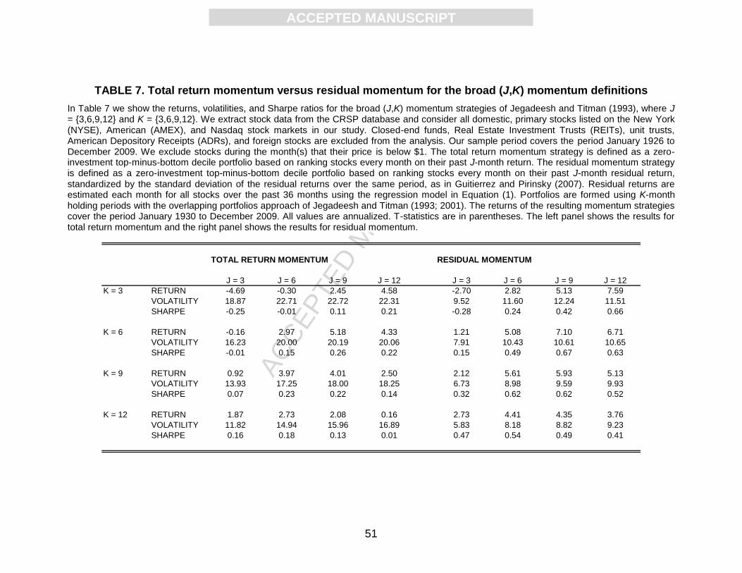
ACC
EPTE
D M
ANU
SCR
IPT
ACCEPTED MANUSCRIPT
51
TABLE 7. Total return momentum versus residual momentum for the broad (J,K) momentum definitions
In Table 7 we show the returns, volatilities, and Sharpe ratios for the broad (J,K) momentum strategies of Jegadeesh and Titman (1993), where J = {3,6,9,12} and K = {3,6,9,12}. We extract stock data from the CRSP database and consider all domestic, primary stocks listed on the New York (NYSE), American (AMEX), and Nasdaq stock markets in our study. Closed-end funds, Real Estate Investment Trusts (REITs), unit trusts, American Depository Receipts (ADRs), and foreign stocks are excluded from the analysis. Our sample period covers the period January 1926 to December 2009. We exclude stocks during the month(s) that their price is below $1. The total return momentum strategy is defined as a zero-investment top-minus-bottom decile portfolio based on ranking stocks every month on their past J-month return. The residual momentum strategy is defined as a zero-investment top-minus-bottom decile portfolio based on ranking stocks every month on their past J-month residual return, standardized by the standard deviation of the residual returns over the same period, as in Guitierrez and Pirinsky (2007). Residual returns are estimated each month for all stocks over the past 36 months using the regression model in Equation (1). Portfolios are formed using K-month holding periods with the overlapping portfolios approach of Jegadeesh and Titman (1993; 2001). The returns of the resulting momentum strategies cover the period January 1930 to December 2009. All values are annualized. T-statistics are in parentheses. The left panel shows the results for total return momentum and the right panel shows the results for residual momentum.
TOTAL RETURN MOMENTUM RESIDUAL MOMENTUM
J = 3 J = 6 J = 9 J = 12 J = 3 J = 6 J = 9 J = 12
K = 3 RETURN -4.69 -0.30 2.45 4.58 -2.70 2.82 5.13 7.59
VOLATILITY 18.87 22.71 22.72 22.31 9.52 11.60 12.24 11.51
SHARPE -0.25 -0.01 0.11 0.21 -0.28 0.24 0.42 0.66
K = 6 RETURN -0.16 2.97 5.18 4.33 1.21 5.08 7.10 6.71
VOLATILITY 16.23 20.00 20.19 20.06 7.91 10.43 10.61 10.65
SHARPE -0.01 0.15 0.26 0.22 0.15 0.49 0.67 0.63
K = 9 RETURN 0.92 3.97 4.01 2.50 2.12 5.61 5.93 5.13
VOLATILITY 13.93 17.25 18.00 18.25 6.73 8.98 9.59 9.93
SHARPE 0.07 0.23 0.22 0.14 0.32 0.62 0.62 0.52
K = 12 RETURN 1.87 2.73 2.08 0.16 2.73 4.41 4.35 3.76
VOLATILITY 11.82 14.94 15.96 16.89 5.83 8.18 8.82 9.23
SHARPE 0.16 0.18 0.13 0.01 0.47 0.54 0.49 0.41
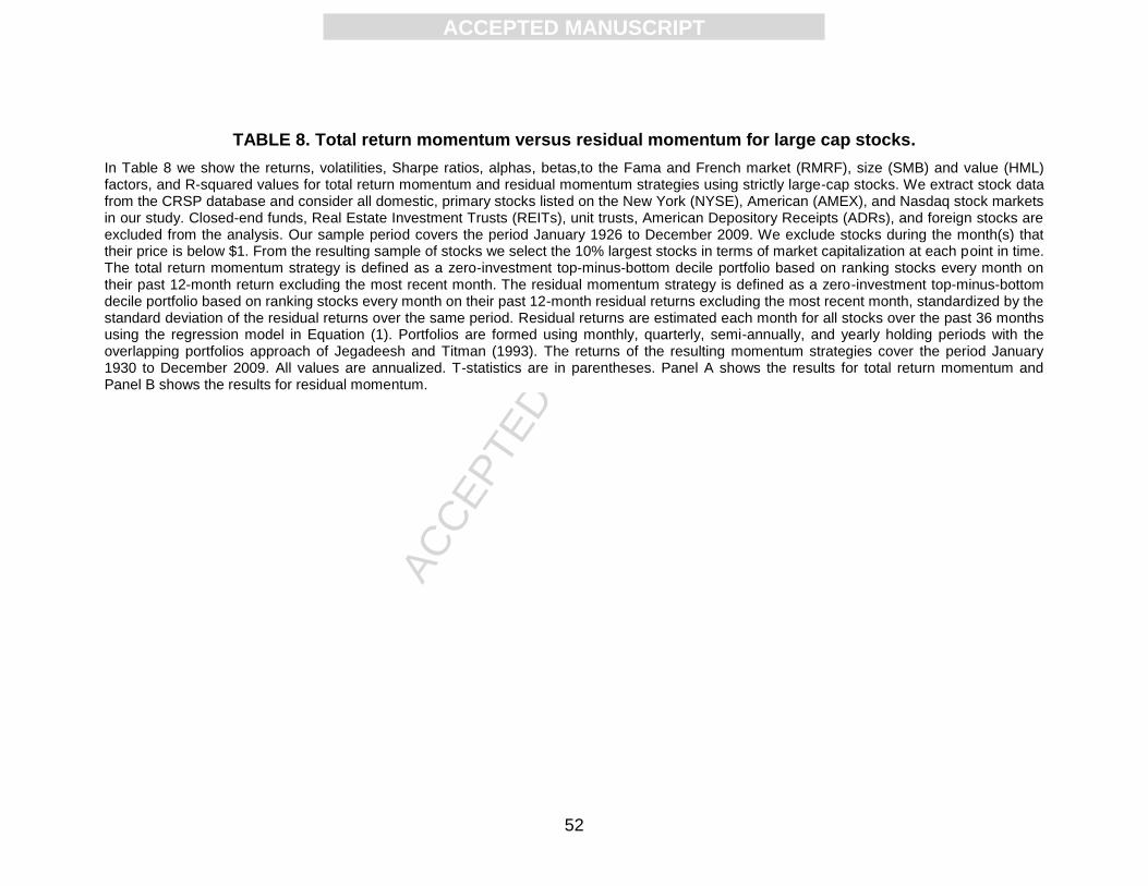
ACC
EPTE
D M
ANU
SCR
IPT
ACCEPTED MANUSCRIPT
52
TABLE 8. Total return momentum versus residual momentum for large cap stocks.
In Table 8 we show the returns, volatilities, Sharpe ratios, alphas, betas,to the Fama and French market (RMRF), size (SMB) and value (HML) factors, and R-squared values for total return momentum and residual momentum strategies using strictly large-cap stocks. We extract stock data from the CRSP database and consider all domestic, primary stocks listed on the New York (NYSE), American (AMEX), and Nasdaq stock markets in our study. Closed-end funds, Real Estate Investment Trusts (REITs), unit trusts, American Depository Receipts (ADRs), and foreign stocks are excluded from the analysis. Our sample period covers the period January 1926 to December 2009. We exclude stocks during the month(s) that their price is below $1. From the resulting sample of stocks we select the 10% largest stocks in terms of market capitalization at each point in time. The total return momentum strategy is defined as a zero-investment top-minus-bottom decile portfolio based on ranking stocks every month on their past 12-month return excluding the most recent month. The residual momentum strategy is defined as a zero-investment top-minus-bottom decile portfolio based on ranking stocks every month on their past 12-month residual returns excluding the most recent month, standardized by the standard deviation of the residual returns over the same period. Residual returns are estimated each month for all stocks over the past 36 months using the regression model in Equation (1). Portfolios are formed using monthly, quarterly, semi-annually, and yearly holding periods with the overlapping portfolios approach of Jegadeesh and Titman (1993). The returns of the resulting momentum strategies cover the period January 1930 to December 2009. All values are annualized. T-statistics are in parentheses. Panel A shows the results for total return momentum and Panel B shows the results for residual momentum.

ACC
EPTE
D M
ANU
SCR
IPT
ACCEPTED MANUSCRIPT
53
TABLE 8. Total return momentum versus residual momentum for large cap stocks (CONTINUED).
RETURN VOLATILITY SHARPE P(RETURN>0) ALPHA RMRF SMB HML RMRF_UP SMB_UP HML_UP ADJ.RSQ
Panel A. Total return momentum
1M 8.87 24.55 0.36 58% 6.30 -0.26 -0.39 -1.15 0.62 0.72 1.31 0.33
(2.75) -(5.19) -(3.56) -(14.93) (8.43) (5.54) (12.08)
3M 7.89 22.30 0.35 58% 5.69 -0.14 -0.38 -1.09 0.53 0.59 1.16 0.31
(2.70) -(3.00) -(3.71) -(15.43) (7.91) (4.96) (11.64)
6M 6.32 21.19 0.30 57% 4.61 -0.07 -0.35 -1.10 0.42 0.58 1.06 0.31
(2.30) -(1.51) -(3.67) -(16.40) (6.59) (5.14) (11.24)
12M 2.34 17.69 0.13 53% 1.93 0.02 -0.25 -0.97 0.28 0.40 0.69 0.31
(1.15) (0.64) -(3.13) -(17.22) (5.23) (4.26) (8.77)
Panel B. Residual momentum
1M 9.18 15.27 0.60 58% 8.92 -0.14 -0.08 -0.25 0.25 -0.03 0.40 0.07
(5.32) -(3.90) -(1.00) -(4.49) (4.67) -(0.35) (5.09)
3M 8.58 14.02 0.61 59% 8.50 -0.11 -0.10 -0.30 0.25 -0.06 0.40 0.09
(5.60) -(3.40) -(1.36) -(5.81) (5.20) -(0.74) (5.57)
6M 6.97 13.19 0.53 58% 7.39 -0.09 -0.16 -0.35 0.19 -0.02 0.40 0.11
(5.23) -(2.83) -(2.41) -(7.46) (4.21) -(0.21) (5.98)
12M 3.86 11.06 0.35 54% 4.37 -0.03 -0.13 -0.29 0.11 0.00 0.26 0.08
(3.62) -(1.18) -(2.16) -(7.08) (2.73) (0.02) (4.48)

ACC
EPTE
D M
ANU
SCR
IPT
ACCEPTED MANUSCRIPT
54
TABLE 9. Incorporating industry effects.
In Table 9 we show the returns, volatilities, Sharpe ratios, alphas, betas to the Fama and French market (RMRF), size (SMB) and value (HML) factors augmented with industry factors, and R-squared values for residual momentum strategies. We extract stock data from the CRSP database and consider all domestic, primary stocks listed on the New York (NYSE), American (AMEX), and Nasdaq stock markets in our study. Closed-end funds, Real Estate Investment Trusts (REITs), unit trusts, American Depository Receipts (ADRs), and foreign stocks are excluded from the analysis. Our sample period covers the period January 1926 to December 2009. We exclude stocks during the month(s) that their price is below $1. The residual momentum strategy is defined as a zero-investment top-minus-bottom decile portfolio based on ranking stocks every month on their past 12-month residual returns excluding the most recent month, standardized by the standard deviation of the residual returns over the same period, as in Guitierrez and Pirinsky (2007). Residual returns are estimated each month for all stocks over the past 36 months using the regression model in Equation (3). The main difference with the analysis reported in Table 2 is that residual returns are estimated relative to a factor model that augments the three Fama and French factors with industry factors. Portfolios are formed using monthly, quarterly, semi-annually, and yearly holding periods with the overlapping portfolios approach of Jegadeesh and Titman (1993; 2001). The returns of the resulting momentum strategies cover the period January 1930 to December 2009. All values are annualized. T-statistics are in parentheses.
RETURN VOLATILITY SHARPE P(RETURN>0) ALPHA RMRF SMB HML RMRF_UP SMB_UP HML_UP ADJ.RSQ
1M 10.42 11.00 0.95 67% 10.06 -0.02 -0.17 -0.33 0.02 0.26 0.40 0.09
(8.41) -(0.65) -(3.03) -(8.09) (0.53) (3.79) (7.16)
3M 9.27 10.21 0.91 67% 9.35 0.01 -0.19 -0.34 0.01 0.19 0.36 0.09
(8.44) (0.36) -(3.51) -(9.05) (0.21) (2.95) (6.96)
6M 7.52 9.12 0.82 65% 7.57 0.04 -0.19 -0.27 -0.01 0.17 0.28 0.07
(7.57) (1.64) -(4.01) -(7.95) -(0.43) (3.04) (5.93)
12M 4.32 7.85 0.55 61% 4.47 0.08 -0.20 -0.21 -0.05 0.13 0.20 0.07
(5.18) (4.43) -(4.75) -(7.34) -(1.88) (2.72) (4.86)

ACC
EPTE
D M
ANU
SCR
IPT
ACCEPTED MANUSCRIPT
55
FIGURE 1. Total return momentum versus residual momentum over time.
Figure 1 shows the cumulative return of total return momentum and residual momentum strategies over time. We extract stock data from the CRSP database and consider all domestic, primary stocks listed on the New York (NYSE), American (AMEX), and Nasdaq stock markets in our study. Closed-end funds, Real Estate Investment Trusts (REITs), unit trusts, American Depository Receipts (ADRs), and foreign stocks are excluded from the analysis. Our sample period covers the period January 1926 to December 2009. We exclude stocks during the month(s) that their price is below $1. The total return momentum strategy is defined as a zero-investment top-minus-bottom decile portfolio based on ranking stocks every month on their past 12-month return excluding the most recent month. The residual momentum strategy is defined as a zero-investment top-minus-bottom decile portfolio based on ranking stocks every month on their past 12-month residual returns excluding the most recent month, standardized by the standard deviation of the residual returns over the same period, as in Guitierrez and Pirinsky (2007). Residual returns are estimated each month for all stocks over the past 36 months using the regression model in Equation (1). Portfolios are formed using monthly holding periods. The returns of the decile portfolios cover the period January 1930 to December 2009.

ACC
EPTE
D M
ANU
SCR
IPT
ACCEPTED MANUSCRIPT
56
FIGURE 1. Total return momentum versus residual momentum over time (CONTINUED).
$0.10
$1.00
$10.00
$100.00
$1,000.00
$10,000.00
1930
1935
1940
1945
1950
1955
1960
1965
1970
1975
1980
1985
1990
1995
2000
2005
Total return momentum Residual momentum

ACC
EPTE
D M
ANU
SCR
IPT
ACCEPTED MANUSCRIPT
57
FIGURE 2. Drawdown of total return momentum versus residual momentum.
Figure 1 shows the drawdown of total return momentum and residual momentum strategies over time, where we define the drawdown at time t as the ratio between the cumulative return of the strategy at time t to the all-time high cumulative return of the strategy up to time t, minus 1. We extract stock data from the CRSP database and consider all domestic, primary stocks listed on the New York (NYSE), American (AMEX), and Nasdaq stock markets in our study. Closed-end funds, Real Estate Investment Trusts (REITs), unit trusts, American Depository Receipts (ADRs), and foreign stocks are excluded from the analysis. Our sample period covers the period January 1926 to December 2009. We exclude stocks during the month(s) that their price is below $1. The total return momentum strategy is defined as a zero-investment top-minus-bottom decile portfolio based on ranking stocks every month on their past 12-month return excluding the most recent month. The residual momentum strategy is defined as a zero-investment top-minus-bottom decile portfolio based on ranking stocks every month on their past 12-month residual returns excluding the most recent month, standardized by the standard deviation of the residual returns over the same period, as in Guitierrez and Pirinsky (2007). Residual returns are estimated each month for all stocks over the past 36 months using the regression model in Equation (1). Portfolios are formed using monthly holding periods. The returns of the decile portfolios cover the period January 1930 to December 2009.

ACC
EPTE
D M
ANU
SCR
IPT
ACCEPTED MANUSCRIPT
58
FIGURE 2. Drawdown of total return momentum versus residual momentum (CONTINUED).
-90%
-80%
-70%
-60%
-50%
-40%
-30%
-20%
-10%
0%
1930
1935
1940
1945
1950
1955
1960
1965
1970
1975
1980
1985
1990
1995
2000
2005
Total return momentum Residual momentum

ACC
EPTE
D M
ANU
SCR
IPT
ACCEPTED MANUSCRIPT
59
FIGURE 3. Monthly performance of total return momentum and residual momentum in 1932 and 2009.
Figure 3 shows the returns of total return momentum and residual momentum over the years 2009 and 1932 per month together with the return on the Fama and French market factor RMRF. We extract stock data from the CRSP database and consider all domestic, primary stocks listed on the New York (NYSE), American (AMEX), and Nasdaq stock markets in our study. Closed-end funds, Real Estate Investment Trusts (REITs), unit trusts, American Depository Receipts (ADRs), and foreign stocks are excluded from the analysis. Our sample period covers the period January 1926 to December 2009. We exclude stocks during the month(s) that their price is below $1. The total return momentum strategy is defined as a zero-investment top-minus-bottom decile portfolio based on ranking stocks every month on their past 12-month return excluding the most recent month. The residual momentum strategy is defined as a zero-investment top-minus-bottom decile portfolio based on ranking stocks every month on their past 12-month residual returns excluding the most recent month, standardized by the standard deviation of the residual returns over the same period, as in Guitierrez and Pirinsky (2007). Residual returns are estimated each month for all stocks over the past 36 months using the regression model in Equation (1). Portfolios are formed using monthly holding periods. The returns of the decile portfolios cover the period January 1930 to December 2009.
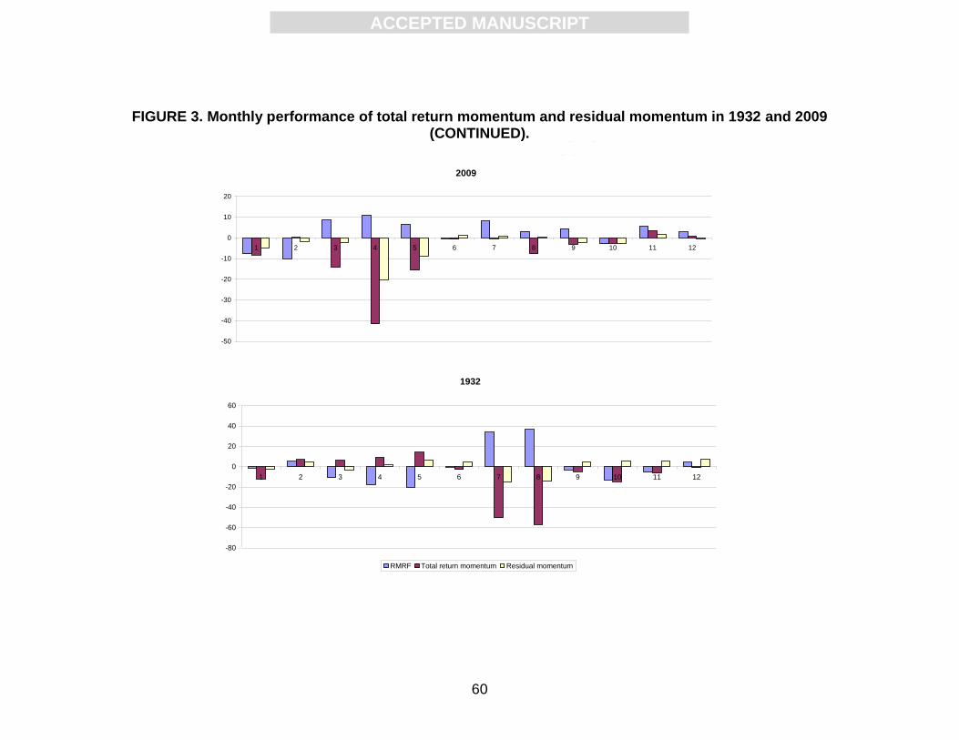
ACC
EPTE
D M
ANU
SCR
IPT
ACCEPTED MANUSCRIPT
60
FIGURE 3. Monthly performance of total return momentum and residual momentum in 1932 and 2009 (CONTINUED).
2009
-50
-40
-30
-20
-10
0
10
20
1 2 3 4 5 6 7 8 9 10 11 12
1932
-80
-60
-40
-20
0
20
40
60
1 2 3 4 5 6 7 8 9 10 11 12
RMRF Total return momentum Residual momentum