resilient virtual topologies in optical networks and clouds · virtual network topology over...
TRANSCRIPT

Resilient virtual topologies in optical
networks and clouds
Minh Bui
A thesis
in
The Department
of
Computer Science and Software Engineering
Presented in Partial Fulfillment of the Requirements
For the Degree of Doctor of Philosophy
Concordia University
Montreal, Quebec, Canada
June 2014
c© Minh Bui, 2014

Concordia University
School of Graduate Studies
This is to certify that the thesis prepared
By: Mr. Minh Bui
Entitled: Resilient virtual topologies in optical networks and
clouds
and submitted in partial fulfillment of the requirements for the degree of
Doctor of Philosophy (Computer Science)
complies with the regulations of this University and meets the accepted standards
with respect to originality and quality.
Signed by the final examining committee :
Chair
Dr. Hashem Akbari
Examiner
Dr. Anjali Agarwal
Examiner
Dr. Terry Fancott
Examiner
Dr. Hovhannes Harutyunyan
External Examiner
Dr. Mario Pickavet
Supervisor
Dr. Briggite Jaumard
Approved by Graduate Program Director
Dr. Volker Haarslev
2014.
Dr. Christopher Trueman
Dean of Faculty
(Engineering and Computer Science)

Abstract
Resilient virtual topologies in optical networks and clouds
Minh Bui, Ph.D.
Concordia University, 2014
Optical networks play a crucial role in the development of Internet by providing a
high speed infrastructure to cope with the rapid expansion of high bandwidth de-
mand applications such as video, HDTV, teleconferencing, cloud computing, and so
on. Network virtualization has been proposed as a key enabler for the next genera-
tion networks and the future Internet because it allows diversification the underlying
architecture of Internet and lets multiple heterogeneous network architectures coexist.
Physical network failures often come from natural disasters or human errors, and
thus cannot be fully avoided. Today, with the increase of network traffic and the pop-
ularity of virtualization and cloud computing, due to the sharing nature of network
virtualization, one single failure in the underlying physical network can affect thou-
sands of customers and cost millions of dollars in revenue. Providing resilience for
virtual network topology over optical network infrastructure thus becomes of prime
importance.
This thesis focuses on resilient virtual topologies in optical networks and cloud
computing. We aim at finding more scalable models to solve the problem of designing
survivable logical topologies for more realistic and meaningful network instances while
meeting the requirements on bandwidth, security, as well as other quality of service
such as recovery time.
To address the scalability issue, we present a model based on a column generation
decomposition. We apply the cutset theorem with a decomposition framework and
lazy constraints. We are able to solve for much larger network instances than the ones
in literature. We extend the model to address the survivability problem in the context
of optical networks where the characteristics of optical networks such as lightpaths
and wavelength continuity and traffic grooming are taken into account.
We analyze and compare the bandwidth requirement between the two main ap-
proaches in providing resiliency for logical topologies. In the first approach, called
iii

optical protection, the resilient mechanism is provided by the optical layer. In the
second one, called logical restoration, the resilient mechanism is done at the virtual
layer. Next, we extend the survivability problem into the context of cloud computing
where the major complexity arises from the anycast principle. We are able to solve
the problem for much larger network instances than in the previous studies. More-
over, our model is more comprehensive that takes into account other QoS criteria,
such that recovery time and delay requirement.
iv

To my parents, Bùi Minh Quang and Nguyễn Thị Đại Từ.
v

Acknowledgments
Foremost, I would like to thank my advisor, Professor Brigitte Jaumard, for super-
vising me during the course of this thesis. I am very fortunate to have her as the
advisor. Her work ethnic always intrigues me. I could never make it without her
tremendous support and guidence.
Next, I would like to thank Professor Chris Develder for working with me on the
latter stage of the thesis. Chris is really effective. I would not finish my thesis timely
without his help.
I would like to thank Professors Anjali Agarwal, Terry Fancott, Hovhannes Haru-
tyunyan, and Mario Pickavet for being on my thesis committee and for their feedback
and suggestions.
I would also like to thanks all the people in my lab for being my friends and
sharing with me the good and the bad times during my thesis.
Last but not least, I would like to thank my family for their love and unconditional
support. This thesis is dedicated to them. They are always the source of motivation
for me, helping me go through many difficult times to finish this thesis. For me, no
one can do a better job than my dad in this saying: “A father is a man who expects
his son to be as good a man as he meant to be”.
vi

Contents
List of Figures xiii
List of Tables xiv
Acronyms xv
1 Introduction 1
1.1 Background . . . . . . . . . . . . . . . . . . . . . . . . . . . . . . . . 1
1.1.1 Application-driven network traffic . . . . . . . . . . . . . . . . 1
1.1.2 Layered network architecture . . . . . . . . . . . . . . . . . . 1
1.1.3 Evolution of optical networks . . . . . . . . . . . . . . . . . . 3
1.1.4 Transition to virtual architectures . . . . . . . . . . . . . . . . 4
1.1.5 Moving to cloud-based services . . . . . . . . . . . . . . . . . 5
1.2 Motivating example . . . . . . . . . . . . . . . . . . . . . . . . . . . . 6
1.3 Thesis contributions . . . . . . . . . . . . . . . . . . . . . . . . . . . 8
1.4 Thesis plan . . . . . . . . . . . . . . . . . . . . . . . . . . . . . . . . 9
2 Background 13
2.1 Optical networks . . . . . . . . . . . . . . . . . . . . . . . . . . . . . 13
2.1.1 Layers of optical networks . . . . . . . . . . . . . . . . . . . . 13
2.1.2 Some concepts and elements of optical networks . . . . . . . . 14
2.1.3 Three generations of optical networks . . . . . . . . . . . . . . 17
2.2 Virtual network architectures . . . . . . . . . . . . . . . . . . . . . . 18
2.2.1 Virtual local area networks . . . . . . . . . . . . . . . . . . . . 19
2.2.2 Virtual private networks . . . . . . . . . . . . . . . . . . . . . 19
2.2.3 Active and software-defined networks . . . . . . . . . . . . . . 19
vii

2.2.4 Overlay networks . . . . . . . . . . . . . . . . . . . . . . . . . 20
2.3 Survivability in optical networks . . . . . . . . . . . . . . . . . . . . . 20
2.3.1 Protection in the optical layer . . . . . . . . . . . . . . . . . . 21
2.3.2 Protection at the logical layer . . . . . . . . . . . . . . . . . . 22
2.4 Techniques to solve large MILP optimization problems . . . . . . . . 23
2.4.1 Available LP/ILP/MILP software . . . . . . . . . . . . . . . . 23
2.4.2 Column generation . . . . . . . . . . . . . . . . . . . . . . . . 23
2.4.3 How to derive an ILP solution . . . . . . . . . . . . . . . . . . 26
3 Literature 32
3.1 Survivable virtual topologies of optical networks . . . . . . . . . . . . 32
3.1.1 The general survivable virtual topologies problem . . . . . . . 32
3.1.2 Different bandwidth granularities . . . . . . . . . . . . . . . . 34
3.2 Optical protection vs. logical restoration . . . . . . . . . . . . . . . . 35
3.3 Virtual survivability in the context of cloud computing . . . . . . . . 37
3.3.1 Anycast request . . . . . . . . . . . . . . . . . . . . . . . . . . 37
3.3.2 QoS support in the context of resiliency for cloud computing . 38
4 Path vs. cutset approaches for the design of logical survivable
topologies 40
4.1 Introduction . . . . . . . . . . . . . . . . . . . . . . . . . . . . . . . . 40
4.2 Statement of the problem and notations . . . . . . . . . . . . . . . . 41
4.2.1 Logical survivable topology design problem . . . . . . . . . . . 41
4.2.2 Notations . . . . . . . . . . . . . . . . . . . . . . . . . . . . . 41
4.2.3 Generalities . . . . . . . . . . . . . . . . . . . . . . . . . . . . 42
4.3 Cutset optimization model . . . . . . . . . . . . . . . . . . . . . . . . 43
4.3.1 Notation . . . . . . . . . . . . . . . . . . . . . . . . . . . . . . 43
4.3.2 Objective function . . . . . . . . . . . . . . . . . . . . . . . . 43
4.3.3 Constraints . . . . . . . . . . . . . . . . . . . . . . . . . . . . 44
4.4 Path optimization model . . . . . . . . . . . . . . . . . . . . . . . . . 44
4.5 Solution of the optimization models . . . . . . . . . . . . . . . . . . . 45
4.5.1 Dealing with an exponential number of cutset constraints . . . 46
4.5.2 Column generation and ILP solution of the models . . . . . . 47
4.5.3 Pricing problems . . . . . . . . . . . . . . . . . . . . . . . . . 48
viii

4.6 Numerical results . . . . . . . . . . . . . . . . . . . . . . . . . . . . . 50
4.7 Conclusions . . . . . . . . . . . . . . . . . . . . . . . . . . . . . . . . 55
5 Logical restoration vs. optical protection: Which one has the least
bandwidth requirement? 57
5.1 Introduction . . . . . . . . . . . . . . . . . . . . . . . . . . . . . . . . 57
5.2 Our contributions . . . . . . . . . . . . . . . . . . . . . . . . . . . . . 59
5.3 IP restoration vs optical protection . . . . . . . . . . . . . . . . . . . 60
5.3.1 Statement of the problem . . . . . . . . . . . . . . . . . . . . 60
5.3.2 Logical restoration vs. optical protection . . . . . . . . . . . . 61
5.4 Optimization models . . . . . . . . . . . . . . . . . . . . . . . . . . . 62
5.4.1 Strategy 1 - Logical restoration . . . . . . . . . . . . . . . . . 62
5.4.2 Strategy 2 - Optical protection . . . . . . . . . . . . . . . . . 68
5.4.3 Strategy 3 - Mixed scheme . . . . . . . . . . . . . . . . . . . . 70
5.5 Solution of the ILP models . . . . . . . . . . . . . . . . . . . . . . . . 70
5.5.1 Strategy 1 . . . . . . . . . . . . . . . . . . . . . . . . . . . . . 71
5.5.2 Strategy 2 . . . . . . . . . . . . . . . . . . . . . . . . . . . . . 72
5.5.3 Strategy 3 . . . . . . . . . . . . . . . . . . . . . . . . . . . . . 72
5.6 Numerical results and analysis . . . . . . . . . . . . . . . . . . . . . . 73
5.6.1 Data instances . . . . . . . . . . . . . . . . . . . . . . . . . . 73
5.6.2 Existence of a survivable logical topology . . . . . . . . . . . . 73
5.6.3 Comparison of the bandwidth requirements: Single link failures 74
5.6.4 Comparison of the bandwidth requirements: Multiple link failures 76
5.7 Conclusions . . . . . . . . . . . . . . . . . . . . . . . . . . . . . . . . 78
6 Design of a survivable VPN topology over a service provider net-
work 80
6.1 Introduction . . . . . . . . . . . . . . . . . . . . . . . . . . . . . . . . 80
6.2 An example . . . . . . . . . . . . . . . . . . . . . . . . . . . . . . . . 83
6.3 Problem statement . . . . . . . . . . . . . . . . . . . . . . . . . . . . 84
6.4 Optimization model . . . . . . . . . . . . . . . . . . . . . . . . . . . . 85
6.4.1 Configurations . . . . . . . . . . . . . . . . . . . . . . . . . . . 85
6.4.2 Master problem . . . . . . . . . . . . . . . . . . . . . . . . . . 86
6.5 Solution of the optimization model . . . . . . . . . . . . . . . . . . . 87
ix

6.5.1 Column generation and ILP solutions . . . . . . . . . . . . . . 87
6.5.2 Pricing problem . . . . . . . . . . . . . . . . . . . . . . . . . . 88
6.5.3 Dealing with exponential number of cutset constraints . . . . 89
6.6 Numerical experiments . . . . . . . . . . . . . . . . . . . . . . . . . . 90
6.6.1 Data instances . . . . . . . . . . . . . . . . . . . . . . . . . . 90
6.6.2 A detailed example solution . . . . . . . . . . . . . . . . . . . 91
6.6.3 Quality of the solutions . . . . . . . . . . . . . . . . . . . . . . 91
6.6.4 Characteristics of the optimized virtual topologies . . . . . . . 94
6.6.5 Single/multi-hop routes vs. number of connected pairs of VPN
nodes . . . . . . . . . . . . . . . . . . . . . . . . . . . . . . . 95
6.6.6 Multi-hop routing versus single hop routing . . . . . . . . . . 98
6.7 Conclusions . . . . . . . . . . . . . . . . . . . . . . . . . . . . . . . . 99
7 Resilience options for provisioning anycast cloud services with vir-
tual optical networks 100
7.1 Introduction . . . . . . . . . . . . . . . . . . . . . . . . . . . . . . . . 100
7.2 Related work . . . . . . . . . . . . . . . . . . . . . . . . . . . . . . . 101
7.3 VNO- vs PIP-resilience . . . . . . . . . . . . . . . . . . . . . . . . . . 103
7.4 Quality of the resilience schemes . . . . . . . . . . . . . . . . . . . . . 105
7.4.1 VNO-resilience . . . . . . . . . . . . . . . . . . . . . . . . . . 105
7.4.2 PIP-resilience . . . . . . . . . . . . . . . . . . . . . . . . . . . 106
7.4.3 Resilience quality options . . . . . . . . . . . . . . . . . . . . 107
7.5 Models for a single synchronization path . . . . . . . . . . . . . . . . 107
7.5.1 Master problem: WB-VNO-resilience . . . . . . . . . . . . . . 108
7.5.2 Master problem: WB-PIP-resilience . . . . . . . . . . . . . . . 110
7.5.3 Pricing problem: WB-VNO-resilience . . . . . . . . . . . . . . 110
7.5.4 Pricing problem: WB-PIP-resilience . . . . . . . . . . . . . . . 112
7.5.5 Improved QoS strategies . . . . . . . . . . . . . . . . . . . . . 113
7.6 Numerical results . . . . . . . . . . . . . . . . . . . . . . . . . . . . . 114
7.6.1 Data sets . . . . . . . . . . . . . . . . . . . . . . . . . . . . . 114
7.6.2 Effect of DC locations and synchronization bandwidth . . . . 117
7.6.3 Effect of disjointness of W and S . . . . . . . . . . . . . . . . 118
7.6.4 Effect of having two synchronization paths . . . . . . . . . . . 118
7.6.5 Effect of the network topology . . . . . . . . . . . . . . . . . . 118
x

7.7 Conclusions . . . . . . . . . . . . . . . . . . . . . . . . . . . . . . . . 119
8 Scalable algorithms for QoS-aware virtual network mapping for cloud
services 121
8.1 Introduction . . . . . . . . . . . . . . . . . . . . . . . . . . . . . . . . 121
8.2 Resilient virtual network mapping with QoS . . . . . . . . . . . . . . 123
8.3 Column generation model: VNO scheme . . . . . . . . . . . . . . . . 126
8.3.1 Master problem . . . . . . . . . . . . . . . . . . . . . . . . . . 126
8.3.2 VNO pricing problem . . . . . . . . . . . . . . . . . . . . . . . 129
8.4 Column generation model: PIP scheme . . . . . . . . . . . . . . . . . 132
8.5 Numerical experiments . . . . . . . . . . . . . . . . . . . . . . . . . . 136
8.5.1 Data instances . . . . . . . . . . . . . . . . . . . . . . . . . . 136
8.5.2 Results . . . . . . . . . . . . . . . . . . . . . . . . . . . . . . . 137
8.6 Conclusions . . . . . . . . . . . . . . . . . . . . . . . . . . . . . . . . 138
9 Conclusion and future work 139
9.1 Conclusions of the thesis . . . . . . . . . . . . . . . . . . . . . . . . . 139
9.2 Future work . . . . . . . . . . . . . . . . . . . . . . . . . . . . . . . . 140
9.2.1 Column generation with heuristic . . . . . . . . . . . . . . . . 140
9.2.2 Dynamic traffic . . . . . . . . . . . . . . . . . . . . . . . . . . 141
Bibliography 155
xi

List of Figures
1.1 The growth of Internet traffic, adapted from [35]. . . . . . . . . . . . 2
1.2 IP-over-WDM network with a virtual layer on top of an optical layer. 3
1.3 An optical network, taken from [127]. . . . . . . . . . . . . . . . . . . 4
1.4 Survivability in an IP-over-WDM network. . . . . . . . . . . . . . . . 7
2.1 Current trend: Moving into IP-over-WDM, adapted from [128]. . . . 14
2.2 Wavelength-division multiplexing. . . . . . . . . . . . . . . . . . . . . 14
2.3 Diagram of an OADM, adapted from [104]. . . . . . . . . . . . . . . . 16
2.4 Diagram of an ROADM, adapted from [104]. . . . . . . . . . . . . . . 16
2.5 An 8x8 optical cross-connect, adapted from [120]. . . . . . . . . . . . 17
2.6 Three generations of optical networks, adapted from [104]. . . . . . . 18
2.7 Protection schemes at the optical layer. . . . . . . . . . . . . . . . . . 22
2.8 Column generation flowchart. . . . . . . . . . . . . . . . . . . . . . . 26
2.9 Branch-and-cut algorithm for solving MILP problems. . . . . . . . . . 28
2.10 Branch-and-price algorithm for solving MILP problems. . . . . . . . . 29
2.11 Complete solution scheme with lazy constraints. . . . . . . . . . . . . 31
4.1 Physical topology. . . . . . . . . . . . . . . . . . . . . . . . . . . . . . 47
4.2 Logical topology. . . . . . . . . . . . . . . . . . . . . . . . . . . . . . 47
4.3 A non survivable mapping. . . . . . . . . . . . . . . . . . . . . . . . . 48
4.4 A survivable mapping. . . . . . . . . . . . . . . . . . . . . . . . . . . 48
4.5 Multiple failure sets in 24-net network. . . . . . . . . . . . . . . . . . 55
5.1 Example about failure dependent backup paths. . . . . . . . . . . . . 68
5.2 Bandwidth requirements of the two scenarios for single link failures
with unit demands. . . . . . . . . . . . . . . . . . . . . . . . . . . . . 76
5.3 Failure sets in 24-net network. . . . . . . . . . . . . . . . . . . . . . 78
xii

6.1 A L1 VPN network. . . . . . . . . . . . . . . . . . . . . . . . . . . . . 82
6.2 Grooming with virtual topology. . . . . . . . . . . . . . . . . . . . . . 85
6.3 Physical topology of German network. Logical nodes are shown in red. 90
6.4 Network flow in a solution. . . . . . . . . . . . . . . . . . . . . . . . . 92
6.5 Total bandwidth between node, note the “near integral” pattern in the
value. . . . . . . . . . . . . . . . . . . . . . . . . . . . . . . . . . . . 93
7.1 Two resilience schemes. . . . . . . . . . . . . . . . . . . . . . . . . . . 104
7.2 Flowchart of the CG ILP approach. . . . . . . . . . . . . . . . . . . . 108
7.3 Experiments on the US topology, for {w, b} disjointness (top), both
{w, b} and {w, s} disjointness (middle), and two synchronization paths
(bottom). . . . . . . . . . . . . . . . . . . . . . . . . . . . . . . . . . 114
7.4 The US topology, as reproduced from [13]. . . . . . . . . . . . . . . . 115
7.5 Experiments on the EU topology for {w, b} disjointness. . . . . . . . 115
7.6 Experiments on the NobelEU network with all possible data center
locations indicated with a star symbol. . . . . . . . . . . . . . . . . . 116
7.7 Distribution of primary and backup DCs on US network. . . . . . . . 119
7.8 Distribution of primary and backup DCs on EU network. . . . . . . . 120
8.1 Two resilience schemes. . . . . . . . . . . . . . . . . . . . . . . . . . . 125
8.2 Decomposition flow chart. . . . . . . . . . . . . . . . . . . . . . . . . 126
8.3 NobelEU network with 4 DC locations indicated with a star symbol. . 133
8.4 Cost distribution. . . . . . . . . . . . . . . . . . . . . . . . . . . . . . 137
xiii

List of Tables
4.1 Description of network instances. . . . . . . . . . . . . . . . . . . . . 50
4.2 Performance of the two models. . . . . . . . . . . . . . . . . . . . . . 51
4.3 Existence of a survivable logical topology. . . . . . . . . . . . . . . . . 52
4.4 Failure sets. . . . . . . . . . . . . . . . . . . . . . . . . . . . . . . . . 53
4.5 Survivability robustness against multiple failures (24-net). . . . . . . 54
5.1 Network topologies. . . . . . . . . . . . . . . . . . . . . . . . . . . . . 73
5.2 Existence of a survivable logical topology. . . . . . . . . . . . . . . . . 74
5.3 Comparison of bandwidth requirements (single-link failures) with unit
demands. . . . . . . . . . . . . . . . . . . . . . . . . . . . . . . . . . 75
5.4 Comparison of bandwidth requirements (single-link failures) with mul-
tiple unit demands. . . . . . . . . . . . . . . . . . . . . . . . . . . . . 75
5.5 Sets of all possible link failures. . . . . . . . . . . . . . . . . . . . . . 77
5.6 Failure scenarios. . . . . . . . . . . . . . . . . . . . . . . . . . . . . . 78
5.7 Comparison of bandwidth requirements (SRLG link failures). . . . . . 79
6.1 Quality of the solutions. . . . . . . . . . . . . . . . . . . . . . . . . . 94
6.2 Characteristics of the generated virtual topologies. . . . . . . . . . . . 95
6.3 Effect of the number of virtual links on the survivability of the network. 96
6.4 Multi-hop routing versus single-hop routing. . . . . . . . . . . . . . . 97
8.1 Cost parameters . . . . . . . . . . . . . . . . . . . . . . . . . . . . . . 136
xiv

Acronyms
ATM asynchronous transfer mode 13
CAPEX capital expenditure 36
CG column generation 23
DC data center 100
ILP integer linear problem 26
LAN local area network 19
LP linear problem 26
MILP mix integer linear problem 23
MPLS multiprotocol label switching 13
O/E/O optical to electronic to optical 13
OADM optical add/drop multiplexer 15
OLT optical line terminal 15
OPEX operating expense 78
OTN optical transport network 13
OXC optical cross connect 16
P2P peer-to-peer 1
PIP physical infrastructure provider 100
PP pricing problem 25
QoS quality of service 122
RMP restricted master problem 24
ROADM reconfigurable optical
add/drop multiplexer 15
RWA routing and wavelength assignment
82
SDN software defined network 19
SLA service level agreement 40
SONET synchronous optical networking
13
SRLG shared risk linked group 37
VLAN virtual local area network 18
VNet virtual network 100
VNO virtual network operator 100
VPN virtual private network 19
WDM wavelength-division multiplexing
14
xv

Chapter 1
Introduction
1.1 Background
1.1.1 Application-driven network traffic
Since its introduction in the early 1980s, Internet has experienced a tremendous
increase in network traffic. From the early 1980s to 2000, Internet traffic has doubled
each year [36]. From 2007 to 2012, the traffic has increased at an annual rate of 46%,
i.e, doubles every two years [34]. It is estimated that there will be nearly 3 billion
Internet users and 14 billion networked devices by 2015 [35].
The network bandwidth increases rapidly to support the high bandwidth demand
of the entertaining applications such as video, HDTV, teleconferencing, social net-
working, file sharing, peer-to-peer (P2P), and so on. These bandwidth-greedy appli-
cations drive the global average broadband speed, which will quadruple from 2010
to 2015. Cisco [35] predicts that the annual global Internet traffic will reach the
zettabyte threshold (≈ 1021 bytes) by the end of 2015.
1.1.2 Layered network architecture
Networks are large and complicated systems, consisting of a number of heterogeneous
network elements. They perform a large variety of communication functions with
equipment from different vendors interworking together. Moreover, networks must
evolve to accommodate the development in the underlying hardware technologies
upon which they are built as well as in the increasing demands of applications. In
1

80
50
60
70
2012The number of households generating over
1 TB per month hits the 1 million mark
2014One-fifth of consumer Internet video now
originates from non-PC devices
2015Internet traffic from wireless devices exceeds
Internet traffic from wired devices
2015The annual run rate of total IP traffic reaches
the zettabyte threshold
2015The number of
networkeddevices is double
pe
r M
on
th
2005
0
10
20
30
40
50
201520102000
2003Consumer Internet surpasses
business Internet
2010Internet video surpasses P2P as the largest
consumer Internet video traffic category
2012Internet video reaches 50 percent consumer
Internet traffic2011
The screensurface area of allconsumer devicesreaches 1 square
foot per capita2011The number of
networked devicesequals the size of the entire global
population
devices is doublethe size of theentire globalpopulation
Exa
by
tes
pe
r M
on
th
Figure 1.1: The growth of Internet traffic, adapted from [35].
order to simplify the management of networks, a layered network architecture is
adopted [104, 126]. The layered network architecture employs a modular design
methodology that decomposes networks into more manageable units.
The general idea of such an approach is that we start with the lowest layer which
corresponds to the underlying hardware and successively build up layer by layer on
top of it. Each layer is designated at a level of abstraction and the higher the layer,
the more abstract it is. Each layer performs a set of functions based on the services
provided by its immediate lower layer and provides a set of services to its immediate
higher layer [102].
Recently, core transport networks have moved into a homogeneous two-layered
model. The upper layer is an IP network employing Multiprotocol Label Switching
(MPLS) and the lower layer is an Optical Transport Network (OTN) running WDM
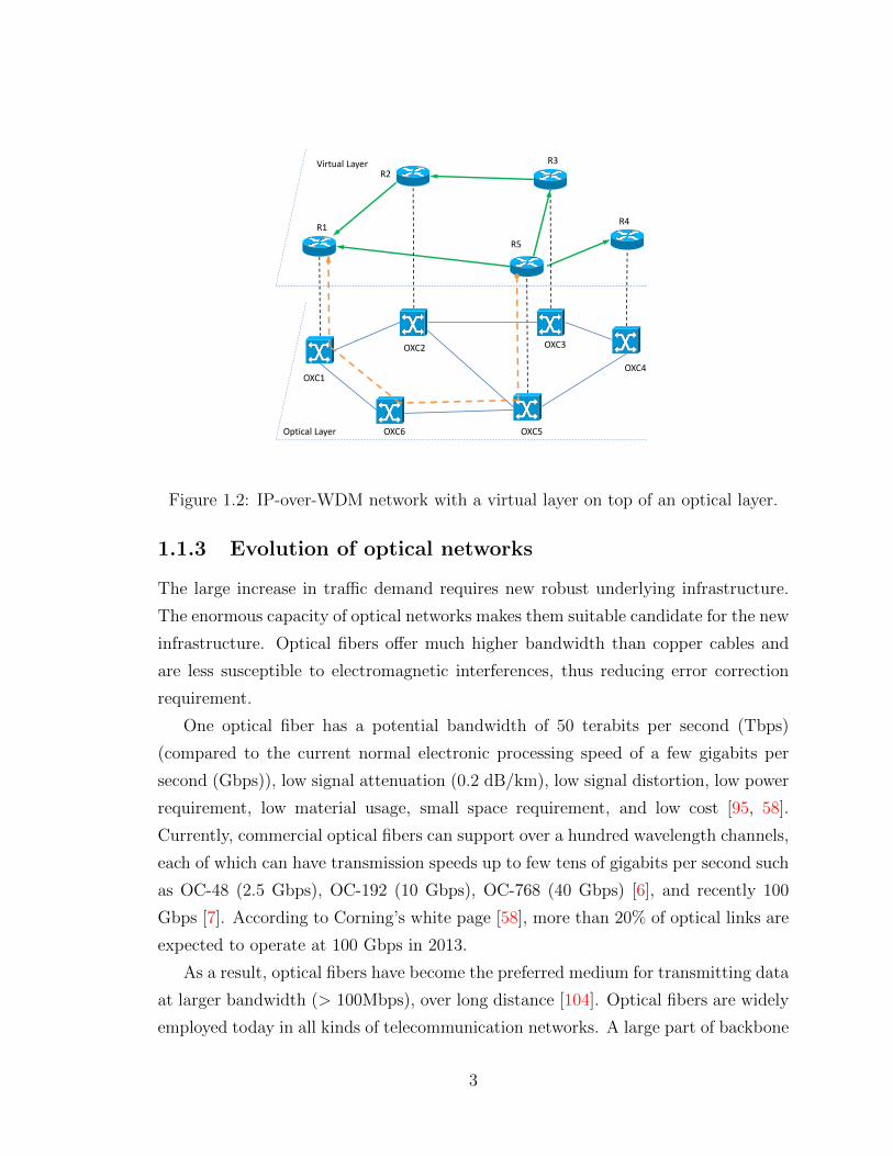
[109, 86, 48]. The IP layer is also referred to as the virtual layer. Figure 1.2 shows
an example of an IP-over-WDM network. In this example, a virtual (i.e., IP) request
from router R5 to R1 will be realized in the optical layer through the path of three
optical cross-connects (OXCs): R5≡OXC5 → OXC6 → OXC1≡R1.
2
Virtual Layer
R1
R2
R3
R4
R5
Optical Layer
OXC2
OXC1
OXC6 OXC5
OXC3
OXC4
Figure 1.2: IP-over-WDM network with a virtual layer on top of an optical layer.
1.1.3 Evolution of optical networks
The large increase in traffic demand requires new robust underlying infrastructure.
The enormous capacity of optical networks makes them suitable candidate for the new
infrastructure. Optical fibers offer much higher bandwidth than copper cables and
are less susceptible to electromagnetic interferences, thus reducing error correction
requirement.
One optical fiber has a potential bandwidth of 50 terabits per second (Tbps)
(compared to the current normal electronic processing speed of a few gigabits per
second (Gbps)), low signal attenuation (0.2 dB/km), low signal distortion, low power
requirement, low material usage, small space requirement, and low cost [95, 58].
Currently, commercial optical fibers can support over a hundred wavelength channels,
each of which can have transmission speeds up to few tens of gigabits per second such
as OC-48 (2.5 Gbps), OC-192 (10 Gbps), OC-768 (40 Gbps) [6], and recently 100
Gbps [7]. According to Corning’s white page [58], more than 20% of optical links are
expected to operate at 100 Gbps in 2013.
As a result, optical fibers have become the preferred medium for transmitting data
at larger bandwidth (> 100Mbps), over long distance [104]. Optical fibers are widely
employed today in all kinds of telecommunication networks. A large part of backbone
3

Figure 1.3: An optical network, taken from [127].
networks are now optical [114, 101]. (Figure 1.3).
1.1.4 Transition to virtual architectures
Internet succeeds because it supports a vast amount of services and applications.
However, the heterogeneous nature of Internet makes it almost impossible to deploy
any radical architecture change. Because adopting a new architecture would require
the consensus from many parties, most of the changes in Internet architecture are
limited to incremental updates [5]. Network virtualization has been proposed as a
key enabler for the next generation networks and the future Internet because it helps
diversify the Internet architecture and lets multiple heterogeneous network architec-
tures coexist [31].
The basic idea behind network virtualization is to split the roles of the tradi-
tional Internet service providers (ISPs) into two independent entities: the Physi-
cal Infrastructure Provider (PIPs) and the Virtual Network Operator (VNOs). The
PIPs create and manage the physical infrastructure while the VNOs create virtual
networks (VNs) by aggregating resources from multiple PIPs and offer end-to-end
services [121, 29, 15]. Network virtualization provides flexibility, promotes diversity,
guarantees security and improves manageability [29]. According to Jain et al. [67],
the five common reasons for network virtualization are as follows:
Sharing: Multiple users can share a big resource.
Isolation : Users, who share the same resource, are invisible to each others.
4

Aggregation : Multiple small resources can be aggregated into a big one and this
process is transparent to users.
Dynamics: Resource requirements can change over time. Resource reallocation be-
comes easier and more efficient (less over-dimensioning) with virtual resources
than with physical resources.
Ease of management: Managing virtual resources is easier because they are software-
defined and expose a uniform interface through standard abstractions.
The mathematical models that we developed in this thesis are quite generic. While
we focus on IP-over-WDM networks, most of them can be applied on any two-layered
network architecture with the upper layer being the virtual layer and the lower layer
being the physical layer. The physical infrastructure can be any kind of physical
networks such as WDM optical networks, wireless networks, or MPLS networks. The
only exception is Chapter 6 where we do traffic grooming for optical networks and
the wavelength continuity is taken into account.
1.1.5 Moving to cloud-based services
Cloud computing, as an extension of grid computing, distributed computing, and
parallel computing, has been envisioned as the next-generation computing model
[61, 93]. Nowadays, most of the largest IT companies provide some cloud computing
services, notably Amazon Elastic Compute Cloud [4], Google App Engine [56], Mi-
crosoft Windows Azure [88], and Saleforce CRM [111]. According to a recent study
by Alcatel-Lucent [101], by 2014, 80% of all new software will be available as cloud
services with 30% of annual growth in enterprise cloud services.
The rapid development of cloud computing is thanks to its major advantages in on-
demand self-service, ubiquitous network access, location independent resource pooling
and transference of risk [135]. Three main categories of cloud computing services are
Infrastructure-as-a-Service (IaaS), Software as a Service (SaaS) and Platform as a
Service (PaaS). The key characteristic of cloud computing is virtualization. In case of
IaaS, several virtual machines (VMs) can be deployed on one actual physical server.
That virtualization offers the flexibility to dynamically change the resource (i.e., mov-
ing from one VM to other VMs) for better performance and resilience against failures.
5
As most cloud applications are bandwidth-demanding with high reliability require-
ments, optical networks play an important role in providing efficient communication
network infrastructure [43]
1.2 Motivating example
An end-to-end network connection typically travels through many network elements.
Each of these elements can fail at anytime. There are many reasons for these failures
such as power outages, fires, earthquakes, cable cuts, etc. For example, the earthquake
in Taiwan on December 26, 2006 cut off several critical optical fibers and caused severe
interruption of telecommunication services in all Eastern Asia [107]. It is estimated
that long-haul networks annually suffer 3 fiber cuts for every 1000 miles of fiber [104].
As most failures come from natural disasters or human errors, network physical
failures cannot be fully avoided. Today, with the increase of network traffic and the
popularity of virtualization and cloud computing, one single physical failure can affect
many customers and cost millions of dollars in lost revenue. According to Bodik et al.
[17], in 2010, North American businesses collectively lost an estimated $26.5 billions
in revenue due to partial or complete outages of services. On average, unplanned
outages cost $5,000 per minute. Thus, guaranteeing of the survivability of a virtual
infrastructure over a wide area optical network becomes of prime importance.
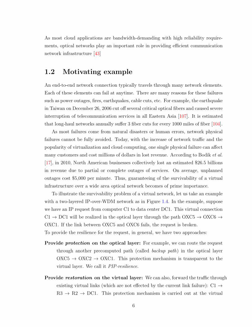
To illustrate the survivability problem of a virtual network, let us take an example
with a two-layered IP-over-WDM network as in Figure 1.4. In the example, suppose
we have an IP request from computer C1 to data center DC1. This virtual connection
C1 → DC1 will be realized in the optical layer through the path OXC5 → OXC6 →OXC1. If the link between OXC5 and OXC6 fails, the request is broken.
To provide the resilience for the request, in general, we have two approaches:
Provide protection on the optical layer: For example, we can route the request
through another precomputed path (called backup path) in the optical layer
OXC5 → OXC2 → OXC1. This protection mechanism is transparent to the
virtual layer. We call it PIP-resilience.
Provide restoration on the virtual layer: We can also, forward the traffic through
existing virtual links (which are not effected by the current link failure): C1 →R3 → R2 → DC1. This protection mechanism is carried out at the virtual
6

Virtual Layer
DC1
R2
R3DC2
C1
R1 R5R4
Optical Layer
OXC2
OXC1
OXC6 OXC5
OXC3
OXC4
Figure 1.4: Survivability in an IP-over-WDM network.
layer (but still needs the collaboration from the optical layer), we call it VNO-
resilience.
In the context of cloud computing, requests are anycast, that is, they can be
served by any data center. If there is a failure in the path from C1 to DC1, including
the failure of DC, we can switch to a backup data center DC2 provided that the
connection between C1 and DC2 is not affected by the failure. Migrating to the
backup data center, however, can raise several real-time synchronization problems
between the two data centers as well as other QoS concerns such as recovery time.
These above problems are indeed optimization problems: How to route the traffic
such that requests are resilient to failures while keeping cost (e.g., total bandwidth,
devices cost) minimum as well as still satisfy some other constraints (e.g., recovery
delay, the bandwidth limit on physical links).
Thanks to its advantages on bandwidth and reliability, optical networks are pre-
ferred hardware infrastructure to deploy virtual networks and cloud applications.
However, optical networks also have their own characteristics that need to be ad-
dressed in the survivability problems. In optical networks, data are sent from sources
to destinations through lightpaths. A lightpath is a connection from a source to a
destination over a unique wavelength. In the above example (Figure 1.4, the path
7

OXC5 → OXC6 → OXC1 is a lightpath at the optical layer. Because the bandwidth
of a lightpath is usually much larger than the traffic requirement of a request, it
would be more economical to group the traffic from different requests to fill up the
bandwidth of a lightpath. This process is called traffic grooming. We also need to
take into account this possibility when planning paths.
As the survivability of a virtual infrastructure becomes more and more impor-
tant, there have been many research efforts on the topic of resilient virtual topolo-
gies. However, to the best of our knowledge, while most of the papers present some
mathematical (i.e., ILP) models, these models are usually too complicated and costly.
Therefore, it is very difficult to apply them on more realistic/meaningful network in-
stances. To address the scalability problem, the authors of these paper propose some
heuristics, which make it difficult to assess the quality of solutions.
The objective of this thesis has three folds:
1. Develop more scalable algorithms to address the survivability problem of virtual
topologies.
2. Add support for traffic grooming in optical networks.
3. Extend the solution to the survivability problem in the context of cloud comput-
ing, while taking into account the characteristics of cloud computing: anycast
requests, recovery time and other different QoS.
1.3 Thesis contributions
This thesis focuses on designing resilient virtual topologies for optical networks and
cloud computing. We aim at finding more scalable ways to design virtual topologies
that are resilient to network failures while meeting requirements on bandwidth, se-
curity, as well as other qualities of service such as recovery time. While this thesis
focuses on optical networks as the physical infrastructures, we can still use the same
technique with other physical infrastructure for the majority of the problems except
for the ones in Chapter 6. The contributions of the thesis include:
• A cutset with a lazy constraint approach for solving the problem of design-
ing survivable topologies for multiple network failures. The algorithm is very
scalable and thus helps solve the problem for much larger network instances
8

compared to previous papers in literature. Results are presented in [69], [70],
and [71].
• A comparison between the performance of the two approaches for designing
survivable optical networks: optical protection and logical restoration. The
results are presented in [68].
• A model to solve the problem of designing survivable VPN topologies. The
main difference in this model compared to the previous one is that the traffic
grooming is taken into account. Papers [20] and [21] present the results.
• Solving the resiliency problem in the context of cloud computing with VNO and
PIP protection scheme. The main difference of the cloud context are: 1. The
requests are anycast. 2. The data center failures are taken into account as well
as recovery time. Results are presented in [22], [24], and [23].
• Adding QoS support to the previous problem. Results are presented in [19] and
[18].
1.4 Thesis plan
This thesis contains five contributing chapters. Each chapter presents a journal article
selected among several papers developed during the course of this PhD thesis. Most of
these articles have already been published or accepted for publication. The remaining
ones are to be submitted to international refereed journals. The detailed organization
of this thesis is as follows:
Chapter 2 provides background knowledge on three areas relating to this thesis:
optical networks, virtual topologies, and large scale optimization. For optical net-
works, we present the basic concepts, terminologies, and essential elements of optical
networks. We also present the general protection mechanisms of optical networks. For
virtual topologies, we present the layered architecture and the general mechanism to
provide resilience in virtual topologies. Finally, for the optimization part, we provide
the basic notion of linear programming and integer programming with the Simplex
algorithm as well as the ideas behind the column generation (CG) and lazy constraint
techniques.
9

Chapter 3 presents a review on the state-of-the-art related work. We focus on the
following points:
1. Scalable algorithms to solve the survivable virtual network topology problem.
2. Survivable virtual network topology problem in the context of optical networks
(lightpath, wavelength continuity)
3. Survivable virtual network topology problem in the context of cloud computing
(data center failures, recovery time, and QoS).
Chapter 4 presents scalable algorithms to solve the classic problem of survivable
virtual network topologies. We present two approaches using decomposition with
the column generation technique, namely path and cutset, to address the scalability
problem. Especially, when using the lazy constraint technique, the cutset algorithm
can solve a much larger network instances compared to the previous examples in
literature.
Chapter 5 presents a comparison in terms of bandwidth requirement between the
two main approaches in solving the network survivability problems: optical protection
vs. logical restoration. In the first approach, which is PIP-based, the resilience is
provided by the optical layer (called optical protection). In the second one, which is
VNO-based, the resilience is handled at the virtual layer (called logical restoration).
Chapter 6 presents a scalable algorithm to solve the problem of designing sur-
vivable virtual topologies in the context of optical networks with the wavelength
continuity and traffic grooming being taken into account.
Chapter 7 solve the resilience problem in the context of cloud computing services
with both the VNO and PIP protection schemes. Requests are presumed anycast and
failures of data centers are taken into account as well as recovery delays.
Chapter 8 extends the problem of chapter 7 by adding QoS support. This takes a
step toward the reality where services, data centers, and infrastructure have different
QoS parameters and requirements.
Chapter 9 concludes the thesis and proposes future work.
The following are the list of the papers that are produced along the course of the thesis:
10

1. B. Jaumard, A. Hoang, and M. Bui. Using decomposition
techniques for the design of survivable logical topologies. In In-
ternational Conference on Advanced Networks and Telecommu-
nication Systems, pages 1–6, December 2011.
Chaper 4
2. B. Jaumard, A. Hoang, and M. Bui. Path vs. cutset ap-
proaches for the design of logical survivable topologies. In IEEE
International Conference on Communications - ICC, pages 1–6,
June 2012.
3. B. Jaumard, A. Hoang, and M. Bui. Two scalable approaches
for the design of logical survivable topologies. IEEE/ACM
Transactions on Networking, 2014. To be submitted.
4. B. Jaumard, M. Bui, B. Mukherjee, and C. Vadrevu. IP
restoration vs. optical protection: Which one has the least band-
width requirements? Optical Switching and Networking - OSN,
10(3):1–30, 2013.
Chaper 5
5. M. Bui, B. Jaumard, C. Cavdar, and B. Mukherjee. Design of
a survivable VPN topology over a service provider network. In
International Conference on Design of Reliable Communication
Networks - DRCN, pages 71–78, March 2013.
Chaper 6
6. M. Bui, B. Jaumard, C. Cavdar, and B. Mukherjee. Scal-
able design of a survivable VPN topology. Journal of Lightwave
Technology, 2014. To be submitted.
11

7. M. Bui, B. Jaumard, and C. Develder. Anycast end-to-end re-
silience for cloud services over virtual optical networks (invited).
In IEEE International Conference on Transparent Optical Net-
works - ICTON, pages 1–7, Cartagena, Spain, June 2013.
Chaper 7
8. M. Bui, B. Jaumard, and C. Develder. Resilience options for
provisioning anycast cloud services with virtual optical networks.
In IEEE International Conference on Communications - ICC,
June 2014.
9. M. Bui, B. Jaumard, and C. Develder. Cost-efficient resilience
for anycast cloud services: virtual vs . physical network layer
resilience optical networks. Journal of Optical Communications
and Networking, 2014. To be submitted.
10. M. Bui, B. Jaumard, I. B. Barla, and C. Develder. Scalable
algorithms for QoS-aware virtual network mapping for cloud ser-
vices. In International Conference on Optical Networking Design
and Modeling - ONDM, May 2014.
Chaper 8
11. M. Bui, B. Jaumard, I. B. Barla, and C. Develder. QoS-
differentiated and resilient virtual network mapping for anycast
cloud services. Journal of Lightwave Technology, 2014. To be
submitted.
12

Chapter 2
Background
2.1 Optical networks
In this chapter we present the basic concepts of optical networks including the layers of
optical networks, the principal network elements and the evolution of optical networks.
2.1.1 Layers of optical networks
In the past, a typical optical network contained a WDM layer as the lowest layer and
synchronous optical networking (SONET), asynchronous transfer mode (ATM), and
IP as the second, third, and top-most layers. This is because conventional WDM
deployment used SONET as standard interface to higher layers and IP packets need
to be mapped into ATM cells before transporting over WDM using SONET frame
[132]. It is also easier to use optical to electronic to optical (O/E/O) conversions at
every node than to build all-optical switches. But this architecture has several disad-
vantages. It is estimated that in WDM/SONET/ATM/IP networks, 22% bandwidth
is used for protocol overhead [132]. Moreover, faster layers are slowed down by slower
layers because layers need to be synchronized. There is also functional overlap since
some layers are duplicating some tasks with respect to routing and protection.
Recently, core transport networks have moved into a homogeneous two-layered
model. The upper layer is an IP network employing multiprotocol label switching
(MPLS) and the lower layer is an optical transport network (OTN) running WDM
[109, 86, 48]. The IP layer is referred to as the virtual layer where each logical link is
mapped to a lightpath (see the definition in Section 2.1.2) in the optical layer .
13

IP/MPLS
IP
Video
Data
Voice
Video
Data
Voice
WDM/OTN
WDM
SDH
ATM
Figure 2.1: Current trend: Moving into IP-over-WDM, adapted from [128].
Fiber Cableλ1
λ2
λ
λ1
λ2
Multiplexer Demultiplexer
λ3
λ4 λ4
λ3
Figure 2.2: Wavelength-division multiplexing.
2.1.2 Some concepts and elements of optical networks
In this section, we present some basic concepts and elements of optical network in-
cluding: wavelength-division multiplexing, lighpath, circuit switching, packet switch-
ing, optical line terminals (OLT), optical amplifiers, optical add/drop multiplexers
(OADM), reconfigurable optical add drop multiplexers (ROADMs), and optical cross-
connects (OXC).
Wavelength-division multiplexing. To exploit the huge capacity of optical fibers,
wavelength-division multiplexing (WDM) is introduced. This technique multi-
plexes a number of optical signals, each corresponds to a wavelength, into a
single optical fiber. See Figure 2.2
Lighpath. In optical networks, data is sent from sources to destinations through
lightpaths. A lightpath is a connection from a source to a destination over a
unique wavelength. Two lightpaths that share some optical link must be on two
different wavelengths.
Circuit switching. In a circuit-switched network, two network nodes establish a
dedicated communication channel (circuit) through the network before the nodes
communicate. A typical example is the early analog telephone network. In
14

circuit-switched optical networks, a lightpath needs to be set up between a
source and a destination, going through dedicated intermediate optical nodes
before the data transmission can be started.
Packet switching. Data in a packet-switched network are divided into packets.
Each packet contains the address of its destination in the packet header. Each
node in the network examines packet headers before forwarding the packets to
the corresponding nodes until the packets reach their destinations.
Optical line terminals. Optical line terminals (OLTs) are deployed at the terminal
points of optical links. On the transmitter side, an OLT adapts incoming electri-
cal signals into optical signals. Each optical signal corresponds to a wavelength.
The OLT combines these signals into an composite optical signal (multiplexing)
that propagates through optical fibers. On the receiver side, an OLT splits in-
coming composite optical signals into several optical signals (demultiplexing),
then converts the optical signals into electrical signals that are usable for clients.
Optical amplifiers. Optical amplifiers are deployed in optical links to deal with the
power attenuation of optical signals by boosting the optical power. However,
they also amplify noise, therefore only a limited number of optical amplifiers
can be put on a link, after that the signal needs to be regenerated using an
optical repeater.
Optical add/drop multiplexers.
Optical add/drop multiplexers (OADMs) are used at the locations where some
lightpaths need to be terminated while others are let through. It can also
add some new lightpath. An OADM has two line ports where the composite
optical signals are present, and several local wavelength ports where individual
lightpaths are dropped and added. Figure 2.3 shows the diagram of an OADM.
Reconfigurable optical add/drop multiplexers.
Reconfigurable optical add/drop multiplexers (ROADMs) are OADMs with
ability to select the desired wavelengths to be dropped and added on the fly.
This feature is made available by Wavelength Selective Switch module as shown
15

λ1, λ2
,…, λw λ1, λ2
,…, λw
Drop Add
Figure 2.3: Diagram of an OADM, adapted from [104].
in Figure 2.4. Normal OADMs only support adding/dropping predefined wave-
lengths. Changing the wavelengths in normal OADMs has to be done locally
and manually, while in ROADMs, the adding/dropping can be done from a re-
mote location. This allows lightpaths to be set up and taken down as needed.
λ1, λ2
,…, λw λ1, λ2
,…, λwWavelength
Selective Switch
Drop Add
Selective Switch
Figure 2.4: Diagram of an ROADM, adapted from [104].
Optical cross-connects. Similar to OADMs, optical cross connects (OXCs) can
selectively add and drop some wavelengths. Besides, they can also switch some
traffic from one optical channel to another [104]. In complex mesh topologies
with a large number of wavelengths and nodes, OXCs are typically put at each
node, sitting between terminating devices and optical networks. Each OXC has
several ports. Some ports are connected to WDM equipments (OLTs) and the
other ports connect to terminating devices such as IP routers. Inside OXCs, the
switch fabric can be optical, electrical, or mixed. One of the most important
features of OXCs is the reconfigurable capability, that is lightpaths can be set
up and torn down as needed, without having to be statically provisioned. Figure
2.5 shows the diagram of a simple 8x8 optical OXC which is able to switch 8
wavelengths (λ1, λ2, ..., λ8) from input ports to 8 wavelengths (λ1, λ2, ..., λ8) in
output ports.
16

Mul
tiple
xer
λ1, λ2
,…, λ8 λ1, λ2
,…, λ8
Dem
ultip
lexe
r
Switch fabric
Dem
ultip
lexe
r
Mul
tiple
xer
λ1, λ2
,…, λ8 λ1, λ2
,…, λ8
Switch fabric
Figure 2.5: An 8x8 optical cross-connect, adapted from [120].
2.1.3 Three generations of optical networks
Along with the development of technology, optical networks have evolved through
several generations. The first generation of optical networks corresponds to point-to-
point systems. They are essentially used for transmission and to provide capacity.
Electrical signals are converted to optical signals at one end, transferred through fiber
links, then converted back to electrical signals at the other end. If the source and
destination are not connected through a lightpath, an optical/electrical conversion is
needed at each intermediate node.
In the first generation networks, all switching and other intelligent network func-
tions were handled by the electronic layer. The electronic devices at a node handled
not only the data intended for that node but also the data that were passed through
that node to other nodes in the network. As data rates increase, it becomes more
difficult for electronic devices to process data at a high speed. If data can be trans-
ferred directly in the optical domain, the burden on the underlying electronics at the
node would be significantly reduced. This is one of the main reason for introducing
the second generation networks [104].
The second generation of optical networks introduces the switching capability. A
lightpath, which is a connection from a source to a destination over the same wave-
length, can be switched over several intermediate nodes in the network. The switch-
ing in the intermediate nodes can be done optically or electrically (circuit switching).
O/E/O conversions are needed for signal regeneration or for switching to another
lightpath (in case data need to be sent over a wavelength path). This is done by
17

1st Generation 2nd Generation
3rd Generation
Figure 2.6: Three generations of optical networks, adapted from [104].
using several optical networking elements like OADM, ROADM, and OXCs. We
describe in detail these network elements in Section 2.1.2.
The third generation optical networks, sometimes called all-optical-networks, is
also experimented. In this generation, data packets can be switched directly in the
optical layer. However optical packet switching is not likely in the near future as
there are still many technical challenges, for example the need of optical RAM to
buffer optical packets. Nowadays, optical networks are effectively a mix between the
first and the second generation.
From the network architecture point of view, the main difference between the
three network generations lays on the switching capability of the optical layer. In the
first generation, there is no switching capability in the optical layer. Circuit switching
is used in the second generation, while in the third generation, packet switching is
used. Figure 2.6 illustrates the differences between the three network generations.
2.2 Virtual network architectures
The idea of virtual networks has been around for a long time. The concept of multiple
coexisting logical networks can be categorized into four main classes: virtual local
area networks (VLANs), virtual private networks (VPNs), active and programmable
18

networks, and overlay networks [29].
2.2.1 Virtual local area networks
A single broadcast domain local area network (LAN) can be partitioned to create
multiple distinct broadcast domains. These domains are connected through routers.
Packets traveling between these domains need to be passed through the routers. Each
packet bears a VLAN ID to enable the routers to forward the packet. A VLAN has the
same attributes as a LAN, but it allows for end stations to be grouped together more
easily. As VLANs provide a higher level of isolation, they help reduce the traffic sent to
unnecessary destinations (i.e., the traffic sending to the stations on the same physical
networks but on different VLANs). VLANs also provide a simpler administration
because all configurations and network management are based on logical instead of
physical connections.
2.2.2 Virtual private networks
A virtual private network (VPN) is a private network that connects multiple sites
using a shared or public network (usually the Internet). The connections between
sites are created using private and secured tunnels. By using Internet, a VPN enables
geographically distributed sites to form a single private network without having to
build private physical infrastructure while still ensuring the security of the network.
2.2.3 Active and software-defined networks
Supporting an increasing demand to add new services to networks or customize ex-
isting networks to meet users’ needs is a complicated and costly process. The main
rational of active and software defined network (SDN) is to simplify the deployment of
new network services, leading to networks that explicitly support the process of service
creation and deployment [25]. The idea of active and programmable networks is that
network devices and flow control is handled by software (programmable interfaces,
network APIs) which is independent from underlying network hardware. By making
network behaviors programmable, active and programmable networks improve op-
erational flexibility, help reduce the cost of building new infrastructure, better use
resource and faster response to emerging security issues.
19

2.2.4 Overlay networks
An overlay network is a network built on the top of another network. Nodes in one
overlay network are connected by virtual links corresponding to a physical path in the
underlying network. For example, peer-to-peer networks are overlay networks built
on top of the Internet. The Internet, in turn, is built as an overlay on the top of
telecommunication networks. Because overlays do not require, nor do they cause any
changes to underlying networks, they have long been used as easy and inexpensive
means to deploy new features and fixes in the Internet [29].
2.3 Survivability in optical networks
Providing resilience against network failures is an important requirement in network
design today. A network connection, between a source to a destination, goes through
several networking components (OLTs, OXCs, OADMs, fibers, routers etc., ). Each
network component can fail during transmission. Examples of the causes of failures
would be power outages, accidental cable cuts, or failures in electrical parts inside
network elements. Network failures can be categorized into node failures (e.g., OXCs,
OADMs, IP routers) and link failures (e.g., fiber-cables cuts and amplifiers). When
a failure occurs, the backup mechanism establishes an alternative path to carry the
interrupted traffic. If the alternative path is computed before the failure occurs,
we refer the technique as protection. If it is computed after the failure occurs (i.e.,
dynamically), we called the backup mechanism as restoration [106]. Both the IP
layer and the optical layer need to be resilient to failure. Restoration mechanisms
are widely deployed at the IP layer, while the optical layer uses both kinds of backup
mechanisms [52].
In order to address all failures without redundancy protection, in the context
of a multi-layer recovery strategy, each layer (IP/optical) is responsible for providing
protection against certain types of failures. The upper layer can provide the protection
for failures in the lower layer if the lower layer can notify the upper layer about the
failures.
If failures occur in IP routers, the recovery must be dealt with by the IP layer.
This is a restoration technique since IP packets are routed over the failed nodes
(i.e., routers) using the routing technology of the IP protocol. If failures occur in
20

the physical layer (e.g., fiber-cable cuts), either the IP layer or the optical layer is
responsible for providing resilience. The optical layer can route the traffic of failed
links over a predefined backup path. The protection at the IP layer is more flexible
but slower than that at the optical layer.
2.3.1 Protection in the optical layer
Protection techniques at the optical layer can provide protection against several types
of network failures such as single-link failures, single link/node failures, and multiple
link failures. Most networks provide protection against single link failures. Some
networks provide protection against node failures and multiple link failures for a
given group of nodes/links, especially in the context of Shared Risk Link Groups
(SRLG).
Protection techniques at the optical layer (i.e., the physical layer) require some
physical redundancy within the network and protocols for rerouting traffic around
the failure using this redundancy. One solution is to have a backup path for every
working path. During normal operation, no traffic or low priority traffic is sent across
the backup path. In case of failure, the higher-priority traffic will be sent over the
backup path. The backup paths are computed before failure happens, thus it is called
protection. To save network capacity reserved for protection, each backup link can
be shared by multiple independent backup paths. Independence means that for a
given failure, those backup paths sharing a link, will not be concurrently used. This
is called shared protection.
Protection schemes can be categorized into three groups, based on the network
structure they intend to protect: path-based schemes, link-based schemes, and segment-
based schemes (Figure 2.7). In general, link-based schemes are faster (as only two
end points of a failed link involve in the restoration process, the rest of the nodes
on a working path can keep the same configuration) but path-based schemes use less
bandwidth (since we use global information to choose a backup path with the cost
almost as good as the working path).
21

(a) Link-based scheme
(c) Segment-based scheme
(b) Path-based scheme
Figure 2.7: Protection schemes at the optical layer.
2.3.2 Protection at the logical layer
The protection at the optical layer, based on some physical redundancy within the
network, is fast since we do not need to go up to the upper layer and do intensive
signaling. If a failure is entirely in the physical layer, it can be handled by protection
at the physical layer. That means, there is no need for protection at the logical layer.
However, while protection at the optical layer is fast and easy to implement, it is
costly. The traffic of an IP request is usually much smaller than the bandwidth of a
wavelength, it would not be economical to use an entire wavelength to protect an IP
request. Moreover, IP requests may have different QoS requirements, it is possible
that some high priority IP requests need protection while others only require best
effort services. Protection at the logical layer can help save cost by offering a more
flexible protection scheme.
When protection in optical networks is not deployed, a network failure (e.g., power
outages, cable cuts) can result in several logical broken links which share the same
physical resource. Those logical broken links, in turn, can make the logical topol-
ogy disconnected. The IP layer has the capability of rerouting traffic, i.e., resilient
to faults if the network (i.e., the logical topology) remains connected. Hence, the
necessary condition for the existence of a restoration scheme at the IP layer is that
22

the logical topology remains connected (survivable) with enough bandwidth in case
of any network failures.
2.4 Techniques to solve large MILP optimization
problems
In this section, we present the general knowledge and techniques to solve mix integer
linear problem (MILP) under the column generation framework.
2.4.1 Available LP/ILP/MILP software
There are a few commercial and open source software (solvers) tools available for
solving LP/ILP/MILP problems. The most popular and well-known commercial
solvers are: IBM ILOG CPLEX Optimization Studio [66]), FICO Xpress [51], and
Gurobi [59]. The most well-known open source ones are GNU Linear Programming
Kit [54], LP SOLVE [55], and COIN-OR LP [37]. A review of these software pro-
grams is presented in [87] with up-to-date performance benchmarks are posted in [90].
Among them, CPLEX seems to be the most well-known and popular.
CPLEX is a powerful optimization software package developed by IBM for linear
programming, mixed integer programming, quadratic programming, and quadrati-
cally constrained programming problems. It is widely used in both academic and in-
dustrial communities. CPLEX supports modeling problems using OPL (Optimization
programming language) that simplifies the formulation and solution of optimization
problems [62]. It has a very rich and powerful feature set as well as an advanced IDE
(Integrated development environment) to help users interfere with the solving process
and adjust algorithms according to their needs. We use CPLEX 12.6 to develop and
run our algorithms on a 4-core 2.2 GHz AMD Opteron 64-bit processor.
2.4.2 Column generation
Column generation (CG) is an efficient technique for solving larger linear programs.
We present here a short introduction to this technique [41, 40]. Column generation
is based on of Dantzig-Wolfe decomposition [38]. Let us start with a general case of
a linear programming problem, called the master problem (MP). We have a linear
23

system of equations of n non-negative variables (x1, x2, · · · xn) and m constraints:
A · x ≥ B
a11x1 + a12x2 + · · · + a1nxn ≥ b1
a21x1 + a22x2 + · · · + a2nxn ≥ b2
......
......
am1x1 + am2x2 + · · · + amnxn ≥ bm
(*)
We need to find the optimal (minimal) value of C · x = c1x1 + c2x2 + . . . cnxn In
many applications n is exponential in m. Therefore, it is not possible to work with
(*) explicitly due to the large size of the problem.
However, in real applications, although the constraint matrix may have a huge size,
it is very rare to find very large models where the non-zeros in the constraint matrix
are greater than 0.1% of the total [119]. In the optimal solution, most of the variables
will be zero (i.e., non-basic variables). These variables, having no influence on the
optimal solution, can be put aside and only a subset of variables need to be considered
when solving the problem. These sub-problems are called restricted master problem
(RMP). For examples, if the optimal solution is X∗ = (x1, x2, . . . , xk, 0, 0, . . . 0) then
we only need to solve the following restricted master problems:
Minimize c1x1 + c2x2 + . . . cnxk
Subject to:
a11x1 + a12x2 + · · · + a1nxk ≥ b1
a21x1 + a22x2 + · · · + a2nxk ≥ b2
......
......
am1x1 + am2x2 + · · · + amnxk ≥ bm
(**)
Obviously, at first, we do not know the which variables need to be taken into
account, but we can find these variables during the course of solving the prob-
lem. Let us solve (*) with the revised simplex method [33]. At any iteration, let
X = (x1, x2, . . . , xk, 0, 0, . . . 0) denote the current feasible solution of MP, the revised
simplex method would proceed as follows:
24

1. Find the dual cost vector π which is the solution of the system of equation
πTABasic = CBasic. Note that π is actually the solution of the dual value of the
current RMP.
2. Compute the reduced cost vector C − πTA to find the entering variable. Any
variable with the strictly negative corresponding cost vector members can enter
the basis. However, since A is very large, we will not compute it explicitly.
Instead, we solve the following optimization problem: Minimize cj−πTaj for aj
is the column j in matrix A and corresponds to variable xj and j ∈ J = {1 . . . n}.This subproblem is called pricing problem (PP).
3. If that optimal value is non-negative then no variable can enter the basis. Thus,
the current solution is optimal, the problem is solved. Otherwise, there is at
least one column j such that cj − πTaj < 0. Variable xj can enter the basis
and becomes non-zero variable and we “add” a new column aj to the master
program.
The CG problem is decomposed into two problems: the master problem and the
pricing problem. The master problem is the original problem with only a subset of
columns being considered, that is, the original problem with only a subset of columns.
The pricing problem is generated and solved at each iteration to find the columns to
be added to the master problem. The objective function of the pricing is generated at
each iteration with respect to the current dual variables. Note that, we do not need
to find the optimal solution in the pricing problem, we only need to find a solution
with a negative reduced cost. That is, we can stop the pricing problem as soon as
the objective value falls below zero and use the incumbent solution.
The CG starts with a feasible solution. It is simple to start with a “dummy”
solution (cold start) - by introducing some artificial columns. Artificial columns
stabilize the column generation procedure as they make the problem remain feasible
while more constraints are added [40]. However, it may be preferable to start with
a closer-to-optimal solution (warm start), since we can expect it can help faster the
convergence of the algorithm. Several heuristics have been used to find a good feasible
initial solution such as: estimation of the optimal dual variable values [1], using a
previous similar run, or a primal heuristic to produce an initial solution [41, 76].
25

Added columns
Dual Values
Restricted Master Problem
Select the best configurations
Yes Reduced
Pricing Problem
Configuration generator
Solve ILP of Restricted Master Problem
Add improving configuration
Optimal LP solution
Reduced cost< 0
No
�-optimal ILP solution
Figure 2.8: Column generation flowchart.
2.4.3 How to derive an ILP solution
In this section, some techniques to improve the efficiency of solving an optimization
model are discussed.
Column management
When the convergence is slow, the number of columns added to the master may
become very large. Having too many columns can create out-of-memory problem
when solving the RMP. In this case, we need to remove some columns from the pool
to keep the number of columns within a limit. The general idea is to remove the
non-basic columns (i.e., the columns associated with zero variables). There are a few
strategies on choosing which column to be removed, for example with the round robin
technique [108]. We can also order the columns by their reduced cost and remove the
columns with a large reduced cost.
Finding ILP solution
In general, we will need to solve an integer linear problem (ILP) problem - a linear
problem with integer variables. First, we solve the optimization model as a linear
26

problem (LP). This problem is called LP relaxation because we leave out the integral
requirements.
After solving the LP relaxation problem, usually we obtain a non-integer solu-
tion. We need to derive an integer solution such that the so-called optimality gap
((zilp − z?lp) /z?lp where z?lp is the optimal value of the LP relaxation, and zilp is the in-
cumbent integer solution) is as small as possible (this corresponds to the second loop
in the scheme). There are several techniques to do this. One of them is using the
rounding off technique, which basically rounds off a non-integer solution to its nearest
integer values. Another one is using a branch-and-cut algorithm for finding integer
solutions [99, 89, 10, 125]. Indeed, internally, CPLEX also uses the combination of
these two techniques therefore we usually let CPLEX derive the integer solution for
us.
Branch-and-cut algorithm
The branch-and-cut algorithm starts after an optimal LP solution is found to get
the lower bound (assuming it is a minimization problem). The problem is split into
multiple sub-problems using some branching scheme. For example, we can branch on
a binary variable x by setting x = 0 or x = 1 on the sub-problems. Next, we solve the
linear programming relaxation of each sub-problem with some cutting plans if needed,
for example we can use Chvatal-Gomory cutting planes [32]. For each problem we get
a lower bound and possibly a upper bound (if the solution is integral). The incumbent
upper bound and lower bound (of the main problem) are updated accordingly. For
any sub-problem, if there is no solution or its solution is greater than the incumbent
upper bound, that branch is pruned. The process is finished when all the branches
are examined. A detailed survey on this method is presented in [99]. Figure 2.9 shows
the flow chart of the algorithm.
Branch-and-price algorithm
The branch-and-price algorithm [11, 42] is a hybrid of the branch-and-bound and
column generation methods. The branch-and-cut algorithm can be used to derive an
integer solution from an optimal LP solution. If the gap between the LP and MILP
solution is too big, we can use branch-and-price algorithm to improve the gap (i.e.,
find a better MILP solution). Usually, the gap is large because there are not enough
27

(all nodes are examined)
Solve LP relaxation (with cutting planes if needed)
Yes
Next
branch
Next node to branch No
Initial minimization problem
Feasible?No
Yes
Prune the node
Optimal MILP solution
Update upper bound
Solution >
bound?
Solution > lower
bound?
Yes
No
Integral solution?No
Update lower bound
Yes
Figure 2.9: Branch-and-cut algorithm for solving MILP problems.
28
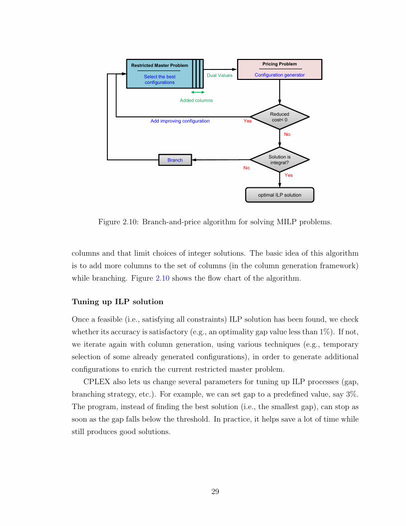
Add improving configuration
Added columns
Dual Values
Restricted Master Problem
Select the best configurations
Yes Reduced cost< 0
No
Pricing Problem
Configuration generator
Branch
optimal ILP solution
Solution is integral?
Yes No
Figure 2.10: Branch-and-price algorithm for solving MILP problems.
columns and that limit choices of integer solutions. The basic idea of this algorithm
is to add more columns to the set of columns (in the column generation framework)
while branching. Figure 2.10 shows the flow chart of the algorithm.
Tuning up ILP solution
Once a feasible (i.e., satisfying all constraints) ILP solution has been found, we check
whether its accuracy is satisfactory (e.g., an optimality gap value less than 1%). If not,
we iterate again with column generation, using various techniques (e.g., temporary
selection of some already generated configurations), in order to generate additional
configurations to enrich the current restricted master problem.
CPLEX also lets us change several parameters for tuning up ILP processes (gap,
branching strategy, etc.). For example, we can set gap to a predefined value, say 3%.
The program, instead of finding the best solution (i.e., the smallest gap), can stop as
soon as the gap falls below the threshold. In practice, it helps save a lot of time while
still produces good solutions.
29

Lazy constraints
When the number of constraints is too large, even with a powerful solver, it is impossi-
ble to include all the constraints into a LP problem. Fortunately, in real applications,
the constraints are usually divided into two categories. The first one (of a small num-
ber) - normal constraints, needed to be included in the set of constraints for finding
the optimal solution. The second one (of a large number), called lazy constraints,
has a special characteristic, that is, only a small number of constraints need to be in-
cluded (and satisfied) explicitly, others are automatically satisfied. Lazy constraints
are introduced to exploit that phenomenon. There is no literature reference avail-
able about this concept although it is well-known in the community of mathematical
programming/CPLEX users.
Treating constraints as lazy constraints means no constraints of the second type
(i.e., lazy ones) need to be included in the set of constraints in the first place. Once
we find the first integer solution, we check whether this solution satisfies all the lazy
constraints. If not, we add the ones that do not meet the constraints (at least some
of them, not necessarily all of them if there are too many) to the current set of
constraints and solve again the newly enriched LP model. Otherwise, we conclude
that we have a feasible integer solution which satisfies all constraints (even if only a
very small fraction of them have been explicitly embedded in the constraint set).
In order to use the lazy-constraints technique, it is crucial to have an algorithm
to check whether there exists any constraint violated, and then identify them in
polynomial time even if there are an exponential number of constraints. This is
called separation problem (see, e.g., [96]).
In practice, only a small number of rounds are sufficient before we get a feasible
integer solution satisfying all constraints.
Solution scheme
The solution scheme is shown in the Figure 2.11. There are three loops in the scheme.
The first one employs the column generation method to solve the LP relaxation
problem. The second loop is to find integer solutions of the problem. The third one
deals with the situations where the gap is too large.
30

No
Yes: Add improving column / configuration
Restricted Master Problem(Minimization)
LP Added columns
Dual Values
Release
Pricing ProblemIf reduced cost < 0
Add (some) violated cutset constraints
Initial Configurations
11
2
Solve ILP of Master
Problem
No
Optimal LP solution
Yes
No�-optimal ILP solution
Release
Selected
Config.All cutsetconstraints satisfied?
Select some configurations
Yes
Optimality gap < �
No
3
Figure 2.11: Complete solution scheme with lazy constraints.
31

Chapter 3
Literature
3.1 Survivable virtual topologies of optical net-
works
The importance of maintaining resilience for virtual topologies in optical networks
leads to a significant amount of work on designing survivable virtual topologies. While
most of the works set out with an ILP (Integer Linear Program) model, in order to
deal with data instances of meaningful sizes, they all move towards applying it on
particular topologies or developing heuristics.
3.1.1 The general survivable virtual topologies problem
In this “classic” problem, the requirements are less stringent. While we still have
the two-layered architecture, there is no specific requirement for the physical layer.
That is, the characteristics of the optical layer e.g., wavelength continuities, lightpath
and bandwidth granularities, etc., are not taken into account. Also, it is purely a
connectivity problem: How to route traffic such that if a failure occurs in the optical
layer, virtual topologies remain connected. The first model is proposed by Modiano
and Narula-Tam [91]. They come up with a necessary and sufficient condition for a
topology to be survivable similar to the max-flow min-cut theorem. They experiment
the condition on some particular topologies (e.g., rings), and relax it to use it on
mesh topologies. Todimala and Ramamurthy [118] improve the ILP model, which
is originally developed by Modiano and Narula-Tam [92], assuming the wavelength
32

continuity condition, subject to SRLG (Shared Risk Link Groups) constraints. The
resulting ILP model is only scalable on particular topologies as its set of constraints
still includes an exponential number of cutsets in the graph underlying virtual topolo-
gies.
To deal with the complexity of designing logical survivable topologies in IP-over-
WDM networks, Kurant and Thiran [79] introduce a mapping from a logical topology
to a simplified one, which preserves the survivability. Such mapping leads them to
a heuristic that efficiently searches for a survivable logical topology over physical
mapping. Their models are then evaluated and enhanced by Javed et al. [74], who
assume that the selected subgraphs, deducted from the logical topology, are cycles.
Thulasiraman et al. [117] study some duality models proposed in [79]. These
models and their previously publish circuit and cutset models have the same al-
gorithmic structures and can be generalized to a new generic cutset model that
removes the distinction between the previous circuit and cutset models. Experi-
ments show that the generic cutset model works more efficiently than the respective
previous models, yet still limited.
Liu and Ruan [85] consider the survivable mapping problem of IP-over-WDM
networks in a more flexible context where several logical links can be added in case
no survivable logical topology exists. Again, the proposed ILP model may not scale
well due to the presence of the exponential number of cutset constraints. Similarly,
Thulasiraman et al. [115] extend their model described in [74] to take into account
the augmented logical links that can be added to ensure the existence of survivable
lightpath routing.
Kan et al. [77] study jointly the capacity assignment and the logical survivability
in IP-over-WDM networks. By taking into account the spare and the working ca-
pacity, they derive some cutset constraints to guarantee the survivability of logical
topologies. Experiments show that lightpath routing has a significant impact on spare
capacity requirements.
Ruiz et al. [109] present a joint approach consisting of over-dimensioning backbone
IP/MPLS nodes and applying lightpath and connectivity restoration. Their solution
introduces new lightpaths in case the topology becomes non-survivable. They propose
an ILP model to resolve the problem but its complexity makes the solution impractical
for real networks. To mitigate the scalability issue, they apply a heuristic based on a
33

genetic algorithm.
Lee et at. [82] study the connectivity problem of layered networks. They propose
a new metric (min-cross-layer cut and weighted-load factor) to measure the connec-
tivity in the networks, then develop several heuristics to make the implementation of
survivable layered networks practical. In [80], they study the similar problem (random
link failures) with probability approach.
In [57], Groebbens et al. study the logical topology design problem for automatic
switched optical networks (ASON). ASONs are capable of increasing/decreasing the
capacity of physical links as well as setting up/tearing down lightpaths on the fly.
Their results show that ASONs are more cost-effective (5 - 15% better) than normal
WDM networks. This is thanks to the dynamic reconfigurability of ASONs that al-
lows resources to be shared dynamically at the time of failure. However, the ASONs
are not widely available at present, for this reason, they are not considered in our sur-
vivability problems which focus on optical networks with static traffic (i.e., planning
perspective).
To date, most of the proposed ILP models are based on the cutset theorem [100],
thus possess a huge number of cutset constraints. As a consequence, many models
become intractable when the size of data instances does not correspond to a (very)
small problem. Among several efforts to reduce the number of generated cutset
constraints by exploiting some special graph structures, so far, none has been able
to deal efficiently with general cases. This is one of the main focuses of the current
study.
3.1.2 Different bandwidth granularities
This section we discus about the survivability problem in a more realistic context of
optical networks where the lightpath bandwidth granularities are taken into account.
Most of the papers in literature about survivable logical topologies consider only the
survivable mapping of one given virtual topology over one physical topology, where
each demand corresponds to only one virtual link. This assumption, however, is
not realistic when connection requests arrive as traffic flows in different bandwidth
granularities. Let us consider the typical example of a global size company requiring
bandwidth in different granularities between a set of network sites. In this multi-layer
architecture, a virtual network of a Layer-1 VPN is setup between several locations.
34

The demanded traffic between two locations is routed over several virtual links by
multi-hop routing.
In [123], Vadrenu et al. suggest to use backup capacity of wavelength services
to support multi-hop IP traffic so that the bandwidth usage is maximized. In [26],
Cavdar et al. study the survivable virtual topology design problem in the context of
multi-hop routing considering both sub-problems at the same time. They present an
ILP model, which is also based on cutset constraints, and solve the problem for only
small networks. Barla et al. [15] propose an MILP model for a very similar problem
but in the context of cloud services with anycast requests. Again, the proposed MILP
model lacks scalability in order to solve meaningful data instances.
In this thesis, we study a similar multi-layer survivable design problem, aiming at
a more scalable solution.
3.2 Optical protection vs. logical restoration
Designing survivable logical topologies for IP-over-WDM networks with the minimum
bandwidth requirement for the mapping of IP (connectivity) requests upon lightpaths,
has been the subject of several studies [91, 118, 79, 85]. In several papers, the authors
focus on the recovery aspect at the logical layer assuming no protection at the optical
layer. Consequently, the papers focus on the connectivity aspect of the logical layer
in IP-over-WDM networks, i.e., ensuring logical networks remain connected in the
face of single or multiple link failure. Readers can refer to [82] for a recent review of
those papers.
We next review the papers concerned with bandwidth requirements in order to
guarantee successful recovery, whether it is optical protection or logical restoration.
Lin et al. [84] add bandwidth requirements in their approach in order to ensure
a 100% successful logical restoration. They distinguish weak survivability, which
stresses on the connectivity aspect of networks, and strong survivability, which takes
into account bandwidth requirements for successful recovery. They propose a two-
stage solution scheme with the help of heuristics, as their ILP models are not tractable.
In their experiments, they assume logical networks are 2-connected whose number of
nodes is half the number of physical nodes. The capacity of each physical link is
given, and the spare capacity is computed on top of that. However, it is not clear
35

how to set the capacity for each physical link (which has a big effect on the final
results).
In [122], Vadrenu et al. suggest to use backup capacity of wavelength services to
support IP traffic so that the bandwidth usage is maximized. IP topology mapping
with guaranteed capacity for IP services has been considered in [124] with backup
capacity sharing between IP and wavelength services.
Kan et al. [77] develop new metrics (load factor and spare factor) for assessing
the quality of logical restoration schemes. They develop two ILP models: one for
maximizing the load factor, the other for minimizing the spare factor. They propose a
joint approach of two stages. In the first stage, they use the first model (i.e., maximize
the load factor) to compute the mapping of the logical links onto the physical ones.
In the second stage, they use the second model (i.e., minimize the spare factor) to
compute the restoration scheme. Their experiments show that lightpath routing has
a significant impact on the spare capacity requirements.
The pros and cons of cross-layer optimization in IP-over-WDM networks are dis-
cussed in Fumagalli et al. [52]. Therein, they propose a heuristic, which allows
varying the percentage of traffic protected by the optical layer and that of traffic rely-
ing on logical restoration, taking into account topology constraints and network cost
minimization. While they discusse the recovery speed and the capital expenditure
(CAPEX) cost, no results on bandwidth requirements are given.
To the best of our knowledge, [110] is the only paper that discusse the bandwidth
requirement for logical restoration vs. those for optical protection in the context
of single link failures. Therein, Sahasrabuddhe et al. compare the two recovery
schemes. For optical protection, the authors consider shared-path protection. For
logical restoration, they propose a routing scheme on two link-independent paths
with some over-dimensioning in order to guarantee that at least one of them is always
operational and able to carry the traffic of the failing path in case of failure. Their
results show that generally optical protection outperforms IP restoration in terms of
required bandwidth and recovery time.
In [50], Dzida et al. propose a decomposition method for solving the IP-over-
WDM survivability problem in case of single-link failure. In the first phase, they
assign physical links to logical links using a shortest path algorithm. In the second
phase, they use a network flow model with a path generation scheme to solve the
36

survivability problem in the logical network.
A different approach to the survivability issues of IP-over-WDM networks is to
use optical protection at the optical layer. In [106], Ramamurthy et al. develop ILP
formulations with shared path protection for single-link failures. In [134], Zang et al.
study single-link failures with shared risk linked group (SRLG) problem with path
protection. They come up with an ILP model (not scalable) and use a heuristic to
mitigate the scalability issue. All the above authors consider single-hop routing only.
In [26], Cavdar et al., for the first time, mention adding multi-hop routing to the
problem. That is, logical topologies are no longer given but need to be built from
traffic demands. They propose an ILP model but the complexity of the model makes
it very difficult to apply even for small network instances. In this thesis, we compare
the bandwidth requirements in order to guarantee a 100% successful IP restoration,
and a 100% optical protection scheme against a set of predefined link failures (which
include all single link failures and some multiple link failures). The comparison is
carried out based on three scenarios: optical protection, logical restoration, and a
mixed one.
3.3 Virtual survivability in the context of cloud
computing
3.3.1 Anycast request
The main difference herein stems from the anycast principle: in a cloud scenario,
we have a certain flexibility in choosing an appropriate data center among a given
set of possible locations to serve the cloud traffic. Thus, the classical notion of a
(source,destination)-based traffic matrix no longer exists [46]. We previously devel-
oped scalable methods, based on the column generation technique to solve the resilient
dimensioning problem: finding working and backup paths for a set of requests as to
always be able to reach an operational data center location [112], even including the
sizing of the data center capacity [44]. However, this previous work does not consider
any resource to accommodate synchronization between distinct working and backup
data center locations.
37

Barla et al. in [15] discuss the VNet planning problem and explain the two re-
silience strategies (VNO- vs. PIP-resilience) and focus on delay minimization, using
mixed integer linear programming (MILP). Optimization of resource cost is treated
by the same authors in [9], but in [9], they do not account for resources used to
synchronize between primary and secondary data centers. Furthermore, those au-
thors also point out that other work optimizes (i) routing cloud service requests and
(ii) mapping a VNet to the physical infrastructure separately. In the problem of sur-
vivable VNet embedding, [81] and [133] consider that the VNet is already designed
and given. In [20, 68], the authors build the most bandwidth-efficient resilient VNet,
under unicast traffic assumptions and using either single or multiple hop routing of re-
quests in the virtual network. In proposing the solutions for optimal server selection,
as well as physical layer routing of anycast services for intra- and inter-DC networks,
the resilience of the resulting virtual layer design is not considered by [75, 3]. It is
important to note that we deal with a planning problem, jointly deciding on multiple
VNets, and not an online VNet mapping that maps one VNet at a time (as in, e.g.,
[131]).
This thesis explicitly addresses solving the resilient VNet design and mapping
problem using simultaneous routing of requests. This is undeniably related to the gen-
eral problem of dimensioning optical cloud/grids: how to find the (minimal) amount
of network and DC resources, to meet a set of given cloud service requests? A ma-
jor complexity problem arises from the anycast principle: we have the flexibility in
choosing a DC among a given set of possible locations. Hence, the classical notion of
a (source,destination)-based traffic matrix disappears [46]. We first develop scalable
methods solve the resilient anycast dimensioning problem [112, 44, 43]. We consider
synchronization between distinct working and backup data center locations initially
in [22] and develop more complete models in [24, 23]. We believe this is the first work
to discuss this in depth.
3.3.2 QoS support in the context of resiliency for cloud com-
puting
As there are more and more applications built upon virtual architectures, each type of
applications has different requirements on the quality and quantity of resource, sup-
porting QoS in cloud computing becomes necessary for any PIP/VNO. Virtualization
38

of cloud infrastructure has been well investigated, both in terms of network planning
[53] (as an offline problem with static traffic) and in terms of traffic engineering [60]
(as an online problem with dynamic provisioning), under anycast routing.
Hao et al. [60] study an aspect of QoS for cloud computing involving the resilience
of data centers. They develop mechanisms to provide seamless migration of virtual
machines in order to guarantee an appropriate QoS in case of failure occurs.
In [15], Barla et al. present a model to provide resilience in both physical and
virtual layers while taking into account the delay requirement. In [12], Baste et
al. extend the model to include the support for a more general QoS criteria. They
consider not only the delay requirement but also other QoS factors such as resource
requirements at virtual nodes, the number of virtual machines, and different costs for
each type of quality. However, their models are not scalable as they can only run for
network instances of very small size (up to 6 virtual nodes).
In this thesis, we aim at providing a more scalable model for the above QoS
problem. This model also provides seamless migration of virtual machines in case of
network and data center failure.
39

Chapter 4
Path vs. cutset approaches for the
design of logical survivable
topologies
4.1 Introduction
The design and the management of the future networks will rely on an all IP-design,
where synergies will need to be developed between the IP and the optical layers in
order to reduce the energy consumption and the network costs, as well as to guarantee
the service level agreement (SLA) while bandwidth greedy applications, like video
services and IPTV services, will continue to grow [16, 64].
Network failures, such as link or node failures, cannot be fully avoided when it
comes to network management. Consequently, a backup mechanism needs to be used
to ensure the network connectivity. When a failure occurs, the backup mechanism
establishes an alternative path to carry the interrupted connections. Depending on
whether this alternative path is generated online or offline, the corresponding backup
mechanism is referred to as restoration or protection, respectively. Restoration mech-
anisms are widely deployed at the IP layer, while the optical layer uses both kinds of
backup mechanisms [52].
The IP layer is referred to as the logical/virtual layer where each logical link is
mapped to a lightpath (i.e., a direct optical connection without any intermediate
electronics) in the optical/physical layer. A network failure, such as a fiber cut, can
40

result in several logical broken links because the physical resource can be shared
among several optical lightpaths, which, in turn, can make the logical topology dis-
connected. Hence, the necessary condition for the existence of a restoration scheme
in the IP layer is that the logical topology remains connected (survivable) in case of
any network failures [39].
In the present study, we revisit the previously proposed optimization models for
the design of logical survivable topologies subject to multiple link failures, and exam-
ine the reasons of their lack of scalability. We then propose two new highly scalable
optimization models, the first one relies on a column generation reformulation of the
previous cutset models, the second one is a new path model based on a flow formu-
lation.
The chapter is organized as follows. Section 4.2 contains a format statement of
the survivable logical topology design problem and the notations. The two newly
proposed mathematical models are described in Section 4.3 and Section 4.4. The key
features of the solution schemes are discussed in Section 4.5. Numerical experiments
are discussed in Section 4.6 follows by conclusions in the last section.
4.2 Statement of the problem and notations
4.2.1 Logical survivable topology design problem
The logical survivable topology design problem is defined as follows. For a given
optical network described by its physical topological, assuming we know the set of
all potential simultaneous link failures and its logical topology, we are interested in
finding a routing (mapping) of each logical link on the physical topology such that:
(i) the mapping cost (bandwidth requirement) is minimized, (ii) the logical topology
remains survivable in case links of a given failure set break down.
4.2.2 Notations
Let the physical topology be represented by a directed graph Gp = (Vp, Ep) where
Vp is the set of nodes, and Ep is the set of links (where each link is associated with a
directional fiber link), where ` denotes a generic physical link. Let the logical topology
represented by a directed graph Gl = (Vl, El) where Vl is the set of nodes, and El is
41

the set of links, where `′ denotes a generic logical link. Each virtual link is associated
with a unit demand. Multi unit demands are therefore represented by a set of links,
making G a multigraph. Let P be the maximum number of port for any node.
For a given logical link `′, let src(`′) be its source node, and dst(`′) be its desti-
nation node. We denote by ω+G(v) (resp. ω−G(v)) the set of outgoing (resp. incoming)
links of node v in graph G.
Let F be the set of potential failure sets, indexed by F , where each set F is a
set of edges (spans) which might fail at the same time (as in a SRLG - Shared Risk
Link Group), where an (undirected) edge {v, v′} encompasses all the directed links
connecting v to v′ or v′ to v. In case of a study on 100% protection against single
physical link failures, each failure set contains a single edge e, and failure sets are
denoted by Fe for e ∈ E, where E denotes the set of spans of Gp, i.e., the pairs of
connected nodes. Consequently,⋃e∈E{Fe} = Ep.
4.2.3 Generalities
The optimization ILP models which we propose rely on the use of wavelength config-
urations, where a wavelength configuration, denoted by c, is a one unit mapping on
a given wavelength λc, and is defined by the list of logical links routed on physical
lightpaths associated with wavelength λc, a lightpath being defined as a connection
carried end to end from source to destination over the same wavelength on each in-
termediate link. More formally, a configuration is characterized by coefficients f c``′
such that f c``′ = 1 if virtual link `′ is routed over physical link ` in configuration c,
i.e., wavelength link (`, λc), 0 otherwise. Parameter ac`′ , equal to 1 if there exists one
lightpath in Gp in configuration c in order to route logical link `′, 0 otherwise. The
value of this parameter can be easily deduced from the information provided by the
configuration characteristic parameters f c``′ .
In the following sections, we present two new ILP models. The first one, called
cutset model, is a decomposition reformulation of the previously proposed ILP models
(e.g., [91, 116, 118]) with a solution scheme (see Section 4.5) which includes a poly-
nomial so-called separation problem to deal with the number of exponential cutset
constraints. The second one, called path model, is another new formulation where
the logical survivability is checked thanks to a set of multi-flow constraints.
42

4.3 Cutset optimization model
4.3.1 Notation
We adapted one of the earliest models we proposed in [70] for the design of a surviv-
able logical topology. We revisited and enhanced it with respect to allow multi-unit
demands in a more efficient way than multiple logical links (instead of a multigraph,
we now use a graph with weighted links). Parameter ac`′ equal to 1 if there is one
lightpath in configuration c for routing logical link `′, 0 otherwise. Indeed,
ac`′ = max`∈Ep
f c``′ . (1)
Parameter ac,F`′ equal to 1 if logical link `′ is impaired following the failure F , 0
otherwise. CS(S, T ) denotes the cutset based on the cut 〈S, T 〉
4.3.2 Objective function
Previously proposed ILP models of the literature only return solutions if and only
if the logical topologies are survivable. However, even a logical topology is not sur-
vivable, it’s still useful to see “how survivable” the logical topology is. For example,
what is the largest number of failure sets such that the logical topology is still surviv-
able. To find the most survivable logical topology, we introduce additional variables
yF`′ and a large penalty coefficient penalNP for not protecting a logical link when a
failure occurs. In our experiments, we use penalNP = 104. Variables yF`′ = 1 if the
traffic on logical link `′ cannot be recovered from a failure of the links of F occurs,
one of the physical links on which `′ is mapped onto belongs to F , following a lack of
connectivity, 0 otherwise.
This model is always feasible, and in the event of a non survivable logical topology,
it provides information on how many logical links cannot be protected. Note that,
since we do not reinforce transport capacity transports, we can always route a logical
link on the physical topology, assuming it is connected.
Configuration variables zc ∈ ZZ+ denotes how many times the configuration c is
used, zc = 0 means that configuration c is not selected.
The objective function can be written:
min∑c∈C
∑`′∈El
f c``′d`′zc + penal×
∑F∈F
∑`′∈El
yF`′ . (2)
43

As the objective function shows, our model first tries to minimize the number of
unprotected tube (logical link, failure set), then minimizes the bandwidth requirement
for mapping logical links.
4.3.3 Constraints
The set of constraints is as follows:∑c∈C
ac`′ zc ≥ d`′ `′ ∈ El (3)∑c∈C
∑`′∈El
∑`∈ω(v)
f c``′d`′zc ≤ P v ∈ Vp (4)
∑c∈C
∑`′′∈CS(S,Vl\S)
ac,F`′′ zc︸ ︷︷ ︸impaired links going through the cutset
≤∑c∈C
∑`′′∈CS(S,Vl\S)
ac`′′ zc︸ ︷︷ ︸links going through the cutset
−1 + yF`′
`′ ∈ El, S ⊂ Vl : `′ ∈ 〈S, Vl \ S〉, F ∈ F (5)
zc ∈ ZZ+ c ∈ C (6)
yF`′ ∈ {0, 1} `′ ∈ El, F ∈ F (7)
Constraints (3) correspond to the demands of the logical links. Constraints (4) set
the limit on the number of port per each node. Constraints (5) are cutset constraints
which check the connectivity, in order to find out whether a restoration path can be
found for logical link `′. Indeed, if a restoration path can be found following a failure of
the links of F impacting `′, one should be able to find an alternate path going through
the cutset CS(S, Vl \S), i.e., there should exists at least one logical link `′′ belonging
to CS(S, Vl\S) such that `′′ is not impaired by the failure of the links of F . The catch
of the constraints (5) is the exponential number of generated constraints. As each
cutset creates a cutset constraints, the number of cutset constraints is proportional
to the number of subset of S, that is 2|S|. This huge number of constraints makes it
very difficult to solve the model directly even for small network instances.
4.4 Path optimization model
The path model and the cutset model differs from one another on constraint set (5),
which is replaced by a set of path constraints, with a multi-flow formulation, in the
44

path model. In order to do so, we introduce another set of variables ϕF`′1`′2∈ {0, 1}
for `′1, `′2 ∈ El and F ∈ F such that ϕF
`′1`′2
is equal to 1 if the restoration path, in
the logical topology, which protects `′1 goes through `′2 in case links of F fail, and 0
otherwise. The set of path constraints can then be written:
ϕF`′1,`′2≤ 1−
∑c∈C
f c``′2zc ` ∈ F, F ∈ F (8)∑
`′2∈ω+Gl
(src(`′1))
ϕF`′1,`′2
=∑
`′2∈ω−Gl
(dst(`′1))
ϕF`′1,`′2
= 1− xF`′1 `′1 ∈ El, F ∈ F (9)
∑`′2∈ω
+Gl
(v)
ϕF`′1,`′2
=∑
`′2∈ω−Gl
(v)
ϕF`′1,`′2
F ∈ F , `′1 ∈ El, v 6∈ {src(`′1),dst(`′1)} (10)
∑`′2∈ω
−Gl
(src(`′1))
ϕF`′1,`′2
=∑
`′2∈ω+Gl
(dst(`′1))
ϕF`′1,`′2
= 0 `′1 ∈ El, F ∈ F (11)
ϕF`′1`′2∈ {0, 1} F ∈ F , `′1, `′2 ∈ El. (12)
Constraints (8) are justified as follows. If logical link `′2 is routed on a physical path
which contains ` (i.e.,∑c∈C
f c``′2zc = 1 in the right hand side of constraints (8)), then
`′2 cannot be used by an alternate route for routing `′1, i.e., ϕF`′1,`′2
= 0, in case failure
F occurs, while ` ∈ F . If xF`′1= 0, i.e., if logical link `′1 can be protected in case
links of failure set F fail, then there is a need for a one unit flow, i.e., 1 − xF`′1 = 1
in constraints (9), from the source to the destination of `′1: this is the purpose of
constraints (9) to (11), which computes a path in the logical graph Gl from src(`′1)
to dst(`′1), for logical link `′1 if it is impacted by failure F . Note that constraints (11)
forbid to consider either incoming links for the source nodes, or outgoing links for
the destination nodes. Otherwise, if xF`′1= 1, logical link `′1 cannot be protected when
failure set F occurs. Thus, no flow can be found for `′1: outgoing flow of source and
incoming flow of destination of `′1 are equal to zero (i.e., 1 − xF`′1 = 0 in constraints
(9)). More detailed information and extended experiments of the path model can be
found at [72].
4.5 Solution of the optimization models
We discuss here how to solve efficiently the two new optimization models described
in the previous section.
45

4.5.1 Dealing with an exponential number of cutset con-
straints
In order to deal with the cutset constraints, we propose to treat them as some so-
called lazy constraints, and then to check for some violated of them using a polynomial
time separation problem, i.e., a problem whose task is to check, for a given solution,
whether the solution satisfies all constraints, and if not, to find a constraint that is
violated by the solution (see, e.g., [129] page 89). Readers can find more detail on
lazy constraints on Section 2.4.3.
Checking cutset constraints
The separation problem (checking cutset constraints) can be easily solved in polyno-
mial time as follows:
Let F ∈ F be a set of physical links that fail simultaneously, and `′ be a logical link.
In order for `′ to be survivable, we need to check whether there always exist a logical
path linking its two endpoints in case the links in F fail. This implies that a given
integer solution corresponds a survivable topology with respect to `′ (`′ is a survivable
logical link) if the set S, i.e., the set of nodes that are reachable via non-failed logical
links from the source src(`′) of `′, contains the destination of `′. This can be easily
done in polynomial time throughout the computation of a shortest path tree using,
e.g., Dijkstra’s algorithm [2]. Otherwise, constraint (5) is violated by the current
integer solution and is added to the current set of constraints.
Let us have a look to an example. The physical topology and logical topology
is depicted in Figure 4.1, Figure 4.2 respectively. One possible mapping is shown in
Figure 4.3. This mapping is non survivable if the physical link (v4, v5) fails. This
can be shown by looking at the cutset 〈{v4}, {v1, v5}〉: as there exists no logical
path connecting the source and destination of `′5 when link (v4, v5) fails, no cutset
constraint, based on this cutset, and requiring there is at most 1 mapped logical link
going through the cutset in order for `′5 to be survivable, can be satisfied. We then
conclude that no survivable logical topology exists without the need to go through or
to add all the cutset constraints. Another mapping, which is survivalbe is shown in
Figure 4.4, this time, we can see that this cutset is also satisfied.
46

v2
v6
v4
v1
v5v
3
Figure 4.1: Physical topology.
v4
v1
v5
Figure 4.2: Logical topology.
4.5.2 Column generation and ILP solution of the models
Column Generation method is nowadays a well known technique for solving efficiently
large scale optimization problems. The challenge lies in the modeling for identifying a
proper decomposition of the original problem into a so-called master problem and one
or several so-called pricing problems. The solution scheme is a two step process where
we first solve the linear relaxation of the master problem1 using column generation
techniques, and then design an algorithm (e.g., rounding off algorithm or the ILP
solution of the restricted master problem) in order to derive an ILP solution such
1In practice, we use a so-called restricted master problem, initialized with a very small set ofinitial configurations, and then enriched it with the promising configurations output by the pricingproblem.
47

v2
v6
v4v1
�'
'2�
�5'
CS =�{v1, v5},{v4}�
v5v3
'1�
�6'
'3�
'4�
Figure 4.3: A non survivable mapping.
v2
v6
v4v1
'1�
�'
'2�
�5'
CS =�{v1, v5},{v4}�
v5v3
�6'
'3�
'4�
Figure 4.4: A survivable mapping.
that the optimality gap (i.e., (zilp − z?lp) /z?lp where z?lp is the optimal value of the
linear relaxation, and zilp is the incumbent ILP solution) is as small as possible. The
last recourse is to use a branch-and-cut algorithm, see, e.g., [33] or [10] if not familiar
with column generation concepts.
4.5.3 Pricing problems
In the context of a column generation algorithm, pricing problems aim at identifying
improving configurations, i.e., configurations which, if added to the current restricted
master problem, will improve the value of the objective of the master problem. Such
configurations correspond to configurations with a so-called negative reduced cost
48

(again, see [33] if not familiar with column generation concepts). We next briefly
outline the pricing problems of the cutset and path models.
Cutset model
The pricing problem is to identify the configuration with negative reduced cost.
cost =∑
(`,`′)∈Ep×El
f c``′d`′ −
∑`′∈El
ud`′a`′ −∑`′∈El
∑`∈ω(v)
upvfc``′d`′
+∑S⊂Vl
∑F∈F
∑`′∈CS(S,VL\S)
∑`′′∈CS(S,VL\S)
uFS,`′(aF`′ − a`′′)
where ud`′ (resp. upv, uFS,`′) are the values of the dual variables associated with con-
straints (3) (resp. (4, 5)).
We setup a network flow for each pair (source/destination) on the physical network,
with f``′ being the flow when no failure occurs and fF``′ being the remaining flow when
F occurs.∑`∈ω+(src(`′))
f``′ =∑
`∈ω−(dst(`′))
f``′ = a`′ `′ ∈ El (13)
∑`∈ω−(src(`′))
f``′ =∑
`∈ω+(dst(`′))
f``′ = 0 `′ ∈ El (14)
∑`∈ω+(v)
f``′ =∑
`∈ω−(v)
f``′ `′ ∈ El, v ∈ V \ {src(`′),dst(`′)} (15)
∑`′∈El
f``′ ≤ 1 ` ∈ Ep (16)
fF``′ = 0 F ∈ F , ` ∈ F, `′ ∈ El (17)∑`∈ω+(src(`′))
fF``′ =
∑`∈ω−(dst(`′))
fF``′ = a`′ − aF`′ `′ ∈ El, f ∈ F (18)
∑`∈ω−(src(`′))
fF``′ =
∑`∈ω+(dst(`′))
fF``′ = 0 `′ ∈ El, f ∈ F (19)
∑`∈ω+(v)
fF``′ =
∑`∈ω−(v)
fF``′ `′ ∈ El, v ∈ V \ {src(`′),dst(`′)} (20)
fF``′ ≤ f``′ F ∈ F , ` ∈ Ep, `′ ∈ El (21)
Constraints (13) - (15) set up a network flow from sources to destinations when
there is no failure. Constraints (16) - (20) set up a network flow from sources to
49

destinations when a failure occurs with the constraints (17) forbid the flow on failed
links. Finally, constraints (21) force the network flows in case of failures lie on the
normal network flows.
Path model
The second pricing is similar but simpler to the pricing problem of the cutset model.
The objective function has changed and there is no flow constraints in case of failures.
See [72] for a detailed model and experiment.
4.6 Numerical results
We conducted experiments on the same four different physical topologies as Todi-
mala and Ramamurthy [118], i.e., NJLATA, NSF, EURO and 24-NET, see Table
4.1. As in [118], we used randomly generated degree k regular undirected graphs
Topologies # nodes# spans = Average nodal
(# links)/2 degree
NJLATA 11 23 4.2
NSF 14 21 3.0
EURO 19 37 3.9
24-NET 24 43 3.4
Table 4.1: Description of network instances.
and m-edge general undirected graphs as virtual topologies. Undirected graphs were
next converted to directed graphs by replacing each span with two opposite directed
links. In Table 4.2, we evaluate the comparative performance of the models model
over one hundred randomly generated virtual topologies of each type (degree k and
m-edge), in the context of single link failures. We provide the average number of
generated/selected configurations, the value of the optimality gap (i.e., accuracy of
the solutions), the mean and the variance of the greatest number of wavelengths that
are used on a link, i.e., an estimation on the number of required wavelengths in order
not to face blocking cases. Both models are able to find ε-solutions with a very small
optimality gap, on average ε < 0.02, meaning provided solutions are optimal from a
practical point of view. With respect to computing times, we observe that both mod-
50

Pat
hM
odel
Cuts
etM
odel
Inst
ance
sT
opo.
#C
onfigu
rati
ons
gap
cpu
#C
onfigu
rati
ons
gap
cpu
#cu
tset
gener
.se
lec.
sec.
gener
.se
lec.
sec.
const
rain
ts
NJL
AT
Adeg
ree
363
.031
.3<
10−
310
9.0
45.8
34.1
0.01
10.3
4.5
20-e
dge
80.2
40.0
<10−
321
2.7
48.1
40.0
<10−
326
.63.
1
NSF
21-e
dge
90.2
42.0
0.01
259.
153
.642
.00.
0359
.45.
7
25-e
dge
109.
150
.0<
10−
343
4.4
57.8
50.0
0.01
110.
23.
4
EU
RO
deg
ree-
311
3.9
55.8
0.02
1,17
2.1
83.7
58.0
0.03
274.
910
.2
30-e
dge
122.
460
.0<
10−
31,
302.
184
.160
.00.
0345
0.1
10.5
35-e
dge
142.
370
.0<
10−
32,
209.
693
.870
.00.
0254
6.8
9.0
24-N
ET
40-e
dge
163.
880
.00.
013,
932.
210
6.2
80.0
0.02
810.
511
.9
45-e
dge
182.
590
.0<
10−
36,
178.
011
3.4
90.0
0.01
1032
.79.
4
Tab
le4.
2:P
erfo
rman
ceof
the
two
model
s.
51

Instances Topo
#survivable # unprotected
topologies (`′, F )
Path Cutset [118] Path Cutset
NJLATAdegree 3 100 100 0 0
20-edge 100 100 0 0
NSF21-edge 98 99 76 3 1
25-edge 100 100 100 0 0
EURO
degree-3 97 99 3 2
30-edge 98 98 5 4
35-edge 100 99 100 0 2
24-NET40-edge 98 97 93 3 1
45-edge 99 99 100 2 2
Table 4.3: Existence of a survivable logical topology.
els are much more scalable than the previously proposed ILP models of the literature
[91, 118], with the cutset model and solution algorithm being much more efficient
than the path ones. The excellent performance of the cutset model lies in the lazy
constraints treatment of the cutset constraints: on average, as indicated in the last
column of Table 4.2, a very small number of cutset constraints need to be explicitly
added before reaching an integer solution which is guaranteed to satisfy them all.
In terms of the existence of a survivable logical topology, results are summarized
in Table 4.3. In the context of single link failures, results are comparable to those
obtained by Todimala and Ramamurthy[118], i.e., most topologies are survivable. In
the last two columns, we have indicated the number of unprotected logical links, when
it is not possible to find a fully survivable logical topology.
In Table 4.5, we look at the relation between the ability to find a survivable logical
topology and the number of logical links, in the context of single and multiple link
failures. The physical topology and failure set are shown in Figure 4.5. The multiple
failure sets are defined in Table 4.4 where Fe, F2 = {F 2
1 , F22 , F
23 }, F 3 = {F 3
1 , F32 },
and F 4 = {F 41 } are the failure sets of single-link failures, dual-link failures, third-link
failures, and fourth link failures, respectively. The indices refer to the node indices
used in Figure 5 of [118]. Experiments were conducted on the 24-net topology
52

Sets Set elements
F 1 Fe = {e}, e ∈ E
F44 = {{2, 6}, {2, 3}} F45 = {{0, 5}, {1, 5}}F46 = {{2, 6}, {3, 6}, {6, 7}} F47 = {{5, 10}, {5, 8}}F48 = {{8, 10}, {8, 11}} F49 = {{9, 12}, {9, 13}}F50 = {{10, 18}, {10, 14}} F51 = {{15, 20}, {15, 21}}F52 = {{15, 16}, {16, 21}} F53 = {{2, 3}, {3, 4}}F54 = {{15, 20}, {21, 20}} F55 = {{14, 15}, {14, 19}}F56 = {{10, 11}, {8, 11}, {12, 11}}F57 = {{8, 10}, {8, 5}, {8, 6}, {8, 9}}F58 = {{12, 13}, {12, 16}} F59 = {{21, 22}, {16, 22}}F60 = {{7, 6}, {7, 9}}F61 = {{0, 5}, {1, 5}, {6, 5}, {5, 8}}
F 2
F 21 = {F44, F45, F47, F48, F49, F50, F51, F52}F 2
2 = F 21 ∪ {F53, F54, F55}
F 23 = F 2
2 ∪ {F58, F59, F60}
F 3 F 31 = {F46} F 3
2 = F 31 ∪ {F56}
F 4 F 41 = {F57} F 4
2 = {F61}
Table 4.4: Failure sets.
for which we generated 10 logical topologies, for a given number of logical links
(randomly generated). For each instance, i.e., for each combination of a given failure
sets (described in the first column) and for each number of randomly generated logical
links (subsequent columns), we reported the number of logical topologies which were
found to be survivable.
While the performances of both models were similar in the context of single link
failures, we found out that, in multiple failure scenarios, the path model was unable to
identify the survivability of some of the logical topologies, i.e., to provide a mapping
of the logical links onto the physical topology which guarantees survivability for all
potential multiple link failures. Indeed, we were unable to get results with the path
model within reasonable computing times for the last failure scenario.
As expected, we observe a reduction in the number of survivable logical topologies
53

#Surv
ivab
leto
lolo
gies
#unpro
tect
ed(`′ ,F
)
Sce
nar
io#
Fai
lure
sets
Pat
hC
uts
etP
ath
Cuts
et
Fe
F2
F3
F4
2030
4050
2030
4050
2030
4050
2030
4050
1Fe
1010
1010
1010
1010
00
00
00
00
2Fe
F2 1
F3 1
910
106
910
1010
20
028
60
00
3Fe
F2 2
F3 2
87
65
810
1010
532
4652
70
00
4Fe
F2 2
F3 2
F4 1
67
65
710
1010
2342
5139
90
00
5Fe
F3 2
F3 2
F4 2
no
resu
lts
afte
r1
day
runnin
g0
01
3-
--
-82
7133
10
Tab
le4.
5:Surv
ivab
ilit
yro
bust
nes
sag
ainst
mult
iple
failure
s(2
4-net
).
54

0
1
6
5
10
118
15 20
14
18
19F45
F47
F48
F50
F51
F54
F55
F56
F57
F61
2
4
3
6
7
12
9
13
21
16
22
17 23
F46F
44
F49
F52F
53
F58
F59
F60
Figure 4.5: Multiple failure sets in 24-net network.
when the number of failure sets increases, i.e., when we look at a column of Table
4.5 from top to bottom. Indeed, few more failure sets may make a whole difference,
see, for instance, the sudden reduction in the number of survivable logical topologies
when going from Scenario 4 to Scenario 5, which differ in four failure sets.
Programs have been developed using OPL and LP/ILP models have been solving
using CPLEX 12.2. Programs were executed on 4-cores 2.2 GHz AMD Opteron 64-bit
processor.
4.7 Conclusions
We proposed and compared two first scalable ILP models for the design of survivable
logical topologies which, thanks to column generation techniques and a polynomial
separation problem for the cutset constraints, allow the exact solution of most of the
data instances considered so far in the literature. The first model, a cutset one, is
significantly better than the second one in terms of runtime performance. In addition,
the cutset model remains very scalable and can still be solved accurately in the context
of higher order failure sets, while the second model has some difficulties identifying
all survivable logical topologies.
In reality, not all traffic between nodes is large enough for setting up direct light-
paths. In chapter 6, we will extend this work to include grooming capability, meaning
55

that small IP traffic between nodes can be groomed into larger IP service traffic de-
mands which correspond to logical links in the current model. In other words, traffic
between two nodes can be transferred thought several IP service demands.
56

Chapter 5
Logical restoration vs. optical
protection: Which one has the
least bandwidth requirement?
5.1 Introduction
IP-over-WDM technology has been envisioned as one of the most attractive network
architectures for the next generation Internet and many studies have already discussed
its potential capabilities. Survivability is a crucial concern in designing IP-over-WDM
networks due to the huge amount of traffic such networks may carry, see, e.g., the
CORONET program [27]. However, large core IP networks do not yet make use of
optical layer reconfigurability, even if the IP network is built on top of an optical layer
network that can be rapidly reconfigured and restored in case of single link failures
[28, 83].
There have been several studies with different assumptions on the recovery schemes.
In general, the studied schemes can be categorized in two types: logical (IP) restora-
tion - where the recovery (i.e., restoration) is carried out in the logical layer and optical
recovery - where the recovery (i.e., protection) is provided by the optical layer. Each
type of recovery has pros and cons. In this paper, we compare the two recovery
approaches over the bandwidth requirements for providing survivability subject to
multiple link failures, which include node failures.
IP-over-WDM networks are being increasingly deployed by network operators in
57

their backbones. They support IP services which include traditional data services
such as VPN, HTTP, data backups, etc. and wavelength services such as terascale
scientific experiments, telemedicine, etc. [14]. With the growing proportion of high-
bandwidth services and the high capacity of optical fiber channels, e.g., 100 Gbps
and beyond, failures in the network such as fiber cuts, node failures, etc., can cause
tremendous loss of capacity. Thus, protection in IP-over-WDM networks against fail-
ures is important for operating a network and also ensuring reliability of the network
services. Two types of failures that are commonly studied are link and node fail-
ures and guaranteeing survivability against single and multiple link/node failures is
crucial.
Two classical strategies for survivability are protection and restoration. In pro-
tection, the backup resources are reserved while, in restoration, they are dynamically
discovered. Protection is ensured at the optical layer while it is restoration at the
logical layer. Optical layer typically comprises of optical cross connects (OXCs) that
are connected with physical fibers and logical layer comprises of IP routers that are
inter-connected with lightpaths. Protection at the optical layer is often dealt with
using path protection, where a primary path is protected by a link (or node)-disjoint
backup path, whether we deal with single link or single link/node failures. In case of
failure of a primary path due a physical link failure, the traffic over the primary path
is switched to the backup path.
A large number of studies on survivable IP-over-WDM networks has focused on
logical restoration only, assuming no optical protection is provided. Logical restora-
tion is assured by enabling connectivity of the logical topology under link and node
(e.g., due to a line card failure) failures. Indeed, if the logical topology is connected,
then the routers can reroute the traffic under failures using IP layer protocols. How-
ever, logical restoration has to face multiple failure cases as multiple lightpaths can be
routed over a single fiber in the physical topology. So, failure of a single physical link
can result in multiple failures in the logical layer and disconnect the logical topology.
Thus, designing a survivable mapping of logical topology over physical topology is a
challenging multi-layer design problem.
To guarantee restorable capacity, we also need to ensure that there is sufficient
excess capacity for the routers to reroute traffic requests under failures. Additional
logical links may be needed in order to ensure either logical connectivity or enough
58

available bandwidth for full recovery of logical requests. In this paper, we are trying
to provide full recovery for logical requests, that is, we are able to send the whole
bandwidth of a disrupted logical request over the restoration path. Depending on
the failure scenarios and traffic patterns (e.g., IP services vs. wavelength services),
it may be more efficient in some situations to ensure protection at the optical layer
and in other situations, with full restoration at the IP layer or with a combination of
both. For those reasons, we decided to investigate in detail the respective bandwidth
requirements of logical restoration vs. optical protection for a given class of services,
i.e., the two extreme cases, under the assumption of single or multiple link/node
failures. We also consider a combination of both recovery types.
The paper is organized as follows. Section 5.2 present our contribution. Section
5.3 describes the detailed statement of the problems that we discuss in this paper
as well as three recovery scenarios in IP-over-WDM networks. Section 5.4 presents
detailed models for computing bandwidth requirement with respect to three recovery
strategies in IP-over-WDM networks. Section 5.6 presents the numerical results,
where we compare and analyze the bandwidth requirements for the three recovery
strategies. Section 5.7 concludes the paper.
5.2 Our contributions
An overview of the recent studies dealing with survivable IP-over-WDM networks,
and especially those studies dealing with the associated bandwidth requirements are
given in Section 3.2. In order to address all failures without recovery redundancy, in
the context of a multi-layer recovery strategy, each layer is responsible for providing
recovery (either protection or restoration) against certain types of failures. For in-
stance, today, failures in the logical layer, e.g., IP routers failures, are dealt with by
the logical layer using logical restoration: IP packets are rerouted around the failed
nodes or line router cards using the route recalculation with either OSPF or IS-IS
protocols.
If failures occur in the physical layer (e.g., fiber-cable cuts or optical cross-connect
failures), the optical layer is usually responsible for it. The traffic going through fail-
ures is sent over predefined backup paths in the optical layer. However, providing pro-
tection in the optical layer may be costly (especially for low-priority, small-bandwidth
59
IP demands), in these cases, protection in the IP layer can be used instead.
We compare the bandwidth requirements of three scenarios, optical protection,
logical restoration and a mixed one. To do so, we propose some exact and scalable
ILP models. For all scenarios, we estimate the bandwidth requirements in order to
guarantee a 100% successful IP restoration, and a 100% optical protection scheme
against a set of predefined link failures (which include all single link failures and
some multiple link failures).
While for recovery against single link failures, it is usually acknowledged that
failure independent path protection offer a good solution, it is no more the case for
multiple failures. Indeed, depending of the number of multiple failures to be protected
against, and the size of the failure sets, it might be difficult, even impossible, to find
a unique protection path for a given working path (lightpath). For this reason, we
turned our attention to multiple path protection schemes (i.e., a failure dependent
path protection scheme) in the case of multiple failures, see, e.g., [103, 98].
5.3 IP restoration vs optical protection
5.3.1 Statement of the problem
The problem of designing a survivable logical topology for IP-over-WDM networks can
be stated as follows: Given an IP-over-WDM network with a list of logical connectivity
demands, (i) how to route these demands onto light-paths and how to map those
light-paths onto the physical layer so that the total required bandwidth is minimum
subject to the condition that the network remains survivable in case of any single or
multiple failure occurs, (ii) how to dimension the logical/physical links in order to
ensure a proper recovery of all logical requests. The three key input elements are:
(i) the failure sets, which can be made of single link failure sets only, but of multiple
link failure ones, including SRLG and node failure sets ; (ii) logical connectivity
demands, which can be single-unit or multiple-unit demands ; and (iii) transport
capacity limits on physical links can also be imposed. We will assign lightpaths to the
logical connectivity demands and route the lightpaths (same wavelength from source
to destination) onto physical routes. Note that the most studied case is with single
link failure sets, single unit logical connectivity demands and did not enforce transport
capacity limits. In the current study, we examine the optical network dimensioning
60

in order to set the transport capacities which guarantee adequate recovery (to be
defined more precisely in Section 5.3.2) for all recoverable IP connectivity requests.
The physical topology is denoted by Gp = (Vp, Ep) where Vp is the set of nodes,
and Ep is the set of physical links (generic index `). The required transport capacity
of link ` is denoted by cap`. The logical topology is denoted by Gl = (Vl, El) where
Vl is the set of nodes, and El is the set of logical links, indexed by `′. Each logical
link `′ has a d`′ ∈ Z+ unit demand, normalized to the bandwidth of a lightpath. Pmaxoxc
is the maximum number of OXC ports for each node.
Let F be the set of all potential failure sets, indexed by F , where each set F is
a set of physical links which might fail at the same time. For single link failures,
each F contains two directed links for each pair of connected nodes. For the failure
of a given node v, the corresponding failure set contains all the (incoming/outgong)
links adjacent to v. For a SRLG (Shared Risk Link Group) failure, F contains all the
failing elements, e.g., all the physical links involved in the same duct. We assume that
F is restricted to maximal failure sets, i.e., failure sets F with F ′ such that F ⊂ F ′
have been eliminated. Note that, a node failure can be accommodated by a collection
of link failures of adjacent links.
5.3.2 Logical restoration vs. optical protection
We investigate the bandwidth requirements for the provisioning of all logical demands
(mapping of the logical links and their demand onto the physical links), and for a
successive recovery (i.e., enough available bandwidth if there is no connectivity issue)
of all logical links in the case of a single or of multiple failures. We consider three
recovery strategies;
• Strategy 1: Pure logical restoration. All failures are recovered through logical
restoration.
• Strategy 2. Pure optical protection. All failures are recovered thanks to optical
protection. In case of router line card failures, it would entail some coordination
between the logical and the optical layers.
• Strategy 3: Mixed recovery. All single link failures (the most common failure in
the optical layer) are recovered through optical protection, while the remaining
failures are recovered thanks to logical restoration.
61

Optical protection will be ensured by shared path protection. In case of multiple
failures, we consider protection paths which might depend on the failure sets, as
in [98], while for single link failures, we can restrict our attention to single path
protection.
For each scenario, we propose to develop an optimization model in order to: (i)
take care of the design of the most survivable logical topology, (ii) compute the band-
width requirements for the mapping of logical links and their demand onto physical
links, (iii) compute the minimum required spare bandwidth for a successful recovery.
By most survivable logical topology, we mean a topology that offers a recovery for
the largest possible number of (`′, F ) pairs, i.e., of logical links (`′) affected by the
failure of the physical links of F . Note that two different logical links `′1, `′2 are not
necessarily altered the same by the F failure scenario. In other words, we are look-
ing for the largest possible protection plan (users should be aware of the failures for
which no recovery can be made). Then, for the largest possible number of pairs, the
recovery plan is with the smallest bandwidth requirements, whether it is restoration
or protection or a mixed recovery scheme.
5.4 Optimization models
We next develop three optimization models, where each model is associated to a given
recovery strategy, see their description in the previous section.
5.4.1 Strategy 1 - Logical restoration
In this recovery, we use logical restoration for protection against single or multiple
link failures. It is a two step solution scheme as in [84], with the difference that
each step is solved exactly instead of heuristically. In addition, we identify the (`′, F )
pairs, made of a logical link and a failure set, which cannot be recovered, rather
than a yes/no approach (the whole logical topology is survivable or is not). The first
step is to find the mapping of the logical links onto the physical links with minimum
bandwidth, as well as identifying the logical links which cannot be recovered due to
a lack of connectivity in the logical layer. In the second step, based on the resulting
mapping, the objective is to optimize the selection of the restoration paths in order
to minimize their bandwidth requirements assuming a shared bandwidth scheme.
62

Step 1. Mapping the logical links onto the physical links
For this first step, we adapted one of the earliest models we proposed in [70] for the
design of a survivable logical topology. We revisited and enhanced it with respect to:
(i) allow multi-unit logical demands in a more efficient way than multiple logical links
(instead of a multigraph, we now use a flow model with multi-unit flows), (ii) detect
the logical links which cannot be mapped onto physical links (due to connectivity
issues: it does not happen if the network is 2-connected, a common assumption); (iii)
compute the bandwidth requirements (capW` ) for proper provisioning of the logical
links with respect to the physical links on which they are mapped.
The ILP model that we propose relies on a decomposition made of configura-
tions defined as follows. Informally, a configuration is made of a collection of non-
overlapping lightpaths, i.e., a point-to-point all-optical wavelength channel path con-
necting the source of a logical link to its destination, all routed over the same wave-
length. Wavelength continuity is guaranteed since each lightpath is entirely defined in
one configuration. Formally, a configuration c is characterized by coefficients f c``′ and
f c` such that f c
``′ = 1 if logical link `′ is routed over physical link ` and f c` =
∑`′∈El
f c``′ ,
i.e., f c` = 1 if physical link ` is used for the routing of a logical link, 0 otherwise.
Parameter ac`′ equal to 1 if there is one lightpath in configuration c for routing logical
link `′, 0 otherwise. Indeed,
ac`′ = max`∈Ep
f c``′ . (22)
Parameter ac,F`′ equal to 1 if logical link `′ is impaired following the failure F , 0
otherwise. CS(S, T ) denotes the cutset based on the cut 〈S, T 〉, where a cut is defined
by the sets of the links going from S to T and such that S, T defines a partition of
Vp.
Variables of the first model are as follows:
63

zc ∈ Z+ Configuration decision variables: zc denotes how many copies
of configuration c are used, zc = 0 means configuration c is
not selected.
capW` ≥ 0 Working bandwidth requirement variables: their values are
equal to the amount of bandwidth on physical link ` so that
all recoverable logical links can be properly dimensioned.
yF`′ ∈ {0, 1} Recovery existence variables: yF`′ = 1 if the traffic on logical
link `′ cannot be recovered from a failure of the links of F
occurs, one of the physical links on which `′ is mapped onto
belongs to F , following a lack of connectivity, 0 otherwise.The objective function can be written:
min∑`∈Ep
capW` + penal×∑F∈F
∑`′∈El
yF`′ . (23)
The first component corresponds to the minimization of the bandwidth requirements
for the mapping of the logical links onto the physical network. To find the most
survivable logical topology, we added second component, weighted with a large penal
parameter, in order to identify the logical demands which cannot be protected from
some given failure sets, in which case yF`′ = 1.
The set of constraints is as follows:∑c∈C
∑`′∈El
f c``′d`′zc ≤ capW` ` ∈ Ep (24)
∑c∈C
ac`′ zc ≥ d`′ `′ ∈ El (25)∑c∈C
∑`′∈El
∑`∈ω(v)
f c``′d`′zc ≤ Pmax
oxc v ∈ Vp (26)
∑c∈C
∑`′′∈CS(S,Vl\S)
ac,F`′′ zc︸ ︷︷ ︸impaired links going through the cutset
≤∑c∈C
∑`′′∈CS(S,Vl\S)
ac`′′ zc︸ ︷︷ ︸links going through the cutset
−1 + yF`′
`′ ∈ El, S ⊂ Vl : `′ ∈ 〈S, Vl \ S〉, F ∈ F (27)
zc ∈ Z+ c ∈ C (28)
yF`′ ∈ {0, 1} `′ ∈ El, F ∈ F (29)
capW` ≥ 0 ` ∈ Ep. (30)
64

Constraints (24), together with the minimization of the objective function takes
care of the evaluation of the bandwidth requirements for a proper provisioning of the
physical links onto which the logical links are mapped. Constraints (25) correspond
to the logical demands of the logical links. Constraints (26) set the limit on the
number of OXC port per each OXC node in the physical network. Constraints (27)
are cutset constraints which check the connectivity, in order to find out whether a
restoration path can be found for logical link `′. Indeed, if a restoration path can be
found following a failure of the links of F impacting `′, one should be able to find
an alternate path going through the cutset CS(S, Vl \ S), i.e., there should exists at
least one logical link `′′ belonging to CS(S, Vl \ S) such that `′′ is not impaired by
the failure of the links of F , or otherwise yF`′ = 1 for the pair (`′, F ).
Step 2: Optimization of the selection of the logical restoration paths
Assuming we are given the mapping of the logical links onto the physical links, the
objective is to optimize the selection of the restoration paths in order to minimize
the bandwidth requirements. Recall that the mappings are assumed to be described
by parameters f``′ such that f``′ = 1 if logical link `′ is mapped on a physical path
containing `. We assume that working routing has been made using a unique route
for routing all the traffic of a given logical link `′, i.e., traffic from src(`′) to dst(`′).
We have two sets of variables:ϕF`′1`′2∈ {0, 1} It is equal to 1 if the restoration logical path for protecting
logical link `′1 goes through `′2, and 0 otherwise.
capR` ≥ 0 Bandwidth requirement on physical link ` in order to ensure
enough available bandwidth for a successful recovery of any
of the recoverable logical links.
Let El(F ) be the set of all logical links of El, which are impaired by a failure of
one of the links of F , and El(��F ) be the set of all logical links, which are not impaired
by a failure of one of the links of F .
The objective, i.e., minimization of the bandwidth requirements for a successful
recovery of the recoverable logical links, can be written as follows:
min∑`∈Ep
capR` . (31)
65

Constraints are expressed as follows:∑`′1∈El(F )
∑`′2∈El(�F )
f``′2 D`′1ϕF`′1,`′2≤ capR
` ` ∈ Ep \ F, F ∈ F (32)
ϕF`′1,`′2
= 0 `′1 ∈ El(��F ), `′2 ∈ El, ` ∈ F, F ∈ F (33)
ϕF`′1,`′2
= 0 `′1 ∈ El(F ), `′2 ∈ El(F ), ` ∈ F, F ∈ F (34)∑`′2∈ω
+Gl
(src(`′1))
ϕF`′1,`′2
=∑
`′2∈ω−Gl
(dst(`′1))
ϕF`′1,`′2
= 1 `′1 ∈ E ′l, F ∈ F (35)
∑`′2∈ω
+Gl
(v)
ϕF`′1,`′2
=∑
`′2∈ω−Gl
(v)
ϕF`′1,`′2≤ 1 `′1 ∈ El(F ), F ∈ F ,
v 6∈ {src(`′1),dst(`′1)} (36)∑`′2∈ω
−Gl
(vs)
ϕF`′1,`′2
=∑
`′2∈ω+Gl
(vd)
ϕF`′1,`′2
= 0 `′1 ∈ El(F ), F ∈ F (37)
capR` ≥ 0 ` ∈ Ep (38)
ϕF`′1`′2∈ {0, 1} F ∈ F , `′1, `′2 ∈ El. (39)
In constraints (32), we compute the bandwidth requirements on physical link `,
following a failure of the links of F . We first need to identify all the logical links `′2
which are not impaired by such a failure: it corresponds to the logical links belonging
to El(��F ) as otherwise `′2 cannot be used in a restoration path for a failure involving
the links of F (inner summation). Next, for any impaired logical link (`′1 ∈ El(F )),
we examine their lightpath mapping, and compute the number of times a lightpath
goes through link ` (outer summation). Last, in order to obtain the bandwidth
requirements for restoration on link `, we look at the failure set with the largest
restoration bandwidth requirements (that is where we take into account bandwidth
sharing among the failure sets). Indeed,
capR` = max`∈Ep\F,F∈F
∑`′1∈El(F )
∑`′2∈El(�F )
f``′2 D`′1ϕF`′1,`′2.
In order to estimate the bandwidth requirements, we only need to consider the
logical links which are impaired by a failure on one of the physical links on which
they are mapped: this is the purpose of constraints (33). We next discuss the design
of the required restoration paths. If ` ∈ F belongs to the physical routing path of
logical link `′2 in the selected configurations (i.e.,∑c∈C
f c``′2zc = 1), then logical link `′2
66

cannot be used by an alternate route for routing any logical link, and in particular
`′1, i.e., ϕF`′1,`′2
= 0, in case links of F fail.
If ` ∈ F does not belong to the physical routing path of logical link `′2 in the
selected configurations, then f``′2 = 0 and, consequently, `′2 can be considered in an
alternate route for routing a logical link in case links of F fails.
If∑c∈C
f c``′1zc = 1 and ` ∈ F , logical link `′1 needs an alternate path if links of F fail.
Consequently, there is a need for an alternate path (i.e., a flow) from the source to the
destination of `′1 in case the links of F fails: this is the purpose of constraints (35) to
(37), which computes a path in Gl from src(`′1) to dst(`′1), for logical link `′1 if it is
impacted by failure F . However, if due to a lack of network connectivity, such a path
cannot be found, then xF`′1= 1. Note that constraints (37) forbid to consider both
incoming links for the source nodes, and outgoing links for the destination nodes. If
a mapping has been found for logical link `′1, but no protection is possible, it is taken
care by variable xF`′ in constraints (35).
When dealing with mathematical modeling for restoration paths, one has to worry
about unnecessary loops in the restoration paths. The first type of loops occur at a
node belonging to the restoration paths, and can be alleviated by forcing the incom-
ing/outgoing flows not to exceed 1 (remember that each logical link is associated to
a one unit demand). This is guaranteed thanks to constraints (34) for the source and
destination nodes, and thanks to constraints (36) for the intermediate nodes. The sec-
ond type of loops has to do with isolated loops, which are not connected to restoration
paths. Those are taken care with minimizing bandwidth requirements that override
these loops that would otherwise artificially increase the bandwidth requirements.
Step 3: Computing the overall bandwidth requirements on the physical
links
The overall bandwidth requirements are given by the sum of the working and the
recovery requirements:
cap` = capW` + capR` ,
where
capW =∑`∈Ep
capW` ; capR =∑`∈Ep
capR` .
67

5.4.2 Strategy 2 - Optical protection
We now present the optimization models for optical protection.
Step 1: Mapping the logical links onto the physical links
Mapping can be done using a shortest path routing of the logical links onto the
physical links.
Step 2: Optical protection against all types of failures
For single link failures, a common approach is to setup a link-disjoint backup path
for each working path. This approach has an advantage of having a simple failure
independent backup path for each demand. However, for multiple failure scenarios,
finding a failure independent backup path might be impossible. Let us have a look at
Figure 5.1 with the working path v1 → v2 → v3. If we consider a double link failure
scenario, then the demand cannot be protected using failure independent approach.
However, if we choose failure dependent approach, the demand can be protected
against double link failures. For example, if links v1 → v2, v2 → v3 fail, we choose
backup path v1 → v4 → v3. If links v1 → v2, v4 → v3 fail, we choose backup path
v1 → v5 → v3.
v1
v2 v4 v5
v3
Figure 5.1: Example about failure dependent backup paths.
The ILP model relies on configurations which are backup paths connecting a
source to a destination, where P denotes the overall set of them, indexed by p. It
corresponds to the so-called path diversity model of Orlowski and Pioro [98], also
known as demand-wise shared protection (DSP) [78]. A recent adaptation to FIPP
p-cycles was proposed by Hoang and Jaumard [63], and Jaumard et al. [73].
68

For each failure set F ∈ F and each demand `′ ∈ El, let P F`′ be the set of backup
paths for `′ when the failure of all/one of the links of F occur(s). Let dF`′ be the
amount of bandwidth of `′ being impaired by F .
There are two sets of variables:capP` ≥ 0 Bandwidth requirement for the protection of physical link `.
zp ∈ Z+ where zp is the number of copies of path p ∈ P F`′ selected as
backup paths for `′ when links of F fail.The objective function can be written as follows:
min∑`∈Ep
capP` . (40)
Constraints are expressed as follows:∑p∈PF
`′
zp ≥ dF`′ `′ ∈ El, F ∈ F (41)
∑p∈P :v∈p
zp ≤ Pmaxoxc v ∈ Vl (42)
∑`′∈El:F∩WP`′ 6=∅
∑p∈PF
`′ :`∈p
zp ≤ capP` ` ∈ Ep, F ∈ F (43)
zp ∈ Z+ p ∈ P (44)
capR` ≥ 0 ` ∈ Ep. (45)
Constraints (41) require all the demands are protected with full bandwidth. Con-
straints (42) limit the number of ports used by each node. Constraints (43) ensure
there is enough bandwidth for protection on each physical link `. The last two sets
of constraints define the domains of the variables.
In order to be solved efficiently, the above model needs to be solved using its
column generation structure, i.e., a decomposition structure where the above model
corresponds to the so-called master problem, and where promising paths are gen-
erated thanks to a so-called pricing problem, see, e.g., Chvatal [33] if not familiar
with column generation techniques or generalized linear programming tools. Several
pricing problems will need to be solved in order to, for each demand `′ ∈ El and each
failure set F ∈ F , generate physical paths that connect src(`′) to dst(`′) when links
of F fail.
69

5.4.3 Strategy 3 - Mixed scheme
In this recovery strategy, we use optical protection for the more frequent failures, i.e.,
single link failures and use logical restoration for multiple link failures. Note that, a
node failure is accommodated by a collection of failures of its adjacent links.
Step 1: Design of a logical survivable topology with respect to multiple
link failure
The model is similar to model (23) - (30), except for constraints (27), which should
be limited to F \F `, with F ` being the failure sets associated with single link failures.
Step 2: Computing the bandwidth requirements of the restoration scheme
for multiple link failure recovery
The model is similar to model (31) - (39), except for constraints (32) - (39), which
should be limited to F \F `, with F ` being the failure sets associated with single link
failures.
Step 3: Computing the bandwidth requirements of the optical protection
scheme for link protection
Model is similar to model (40)- (43), except for constraints (41), (43), which should
be limited to F `.
Step 4: Computing the overall bandwidth requirements on the physical
links
cap` = capW` + max{capR` (Step 2), capP` (Step 3)}.
5.5 Solution of the ILP models
We are using column generation technique with lazy constraints to solve the problems
in this chapter. The information relating to CG technique are presented in Section
2.4.2 with lazy constraints technique are detailed in 2.4.3.
70

In the next three paragraphs, we detail the objective (reduced cost) and con-
straints of each of the pricing problems, one for each of the models described in
Section 5.4.
5.5.1 Strategy 1
The pricing problem is to identify a configuration, i.e., a set of lightpaths in a given
wavelength plan, with a negative reduced cost. The analytical expression of the
reduced cost can be written as follows:
cost =∑
(`,`′)∈Ep×El
f c``′d`′ −
∑`′∈El
ud`′a`′ −∑`′∈El
∑`∈ω(v)
upvfc``′d`′
+∑S⊂Vl
∑F∈F
∑`′∈CS(S,VL\S)
∑`′′∈CS(S,VL\S)
uFS,`′(aF`′ − a`′′)
where ud`′ (resp. upv, uFS,`′) are the values of the dual variables associated with con-
straints (25) (resp. (26), (27)).
For the constraints, we need to setup a network flow for each pair (source, desti-
nation) on nodes in the physical network, using the following set of variables:
fF``′ flow variable in order to identify the mapping of the logical links `′
onto the physical links ` when the links of failure set F fail.
f``′ = maxF∈F
fF``′ flow variable in order to identify the mapping of the
logical links `′ onto the physical links `: it is equal to one if ` is used
is a least one restoration path for a given failure set, 0 otherwise.
∑`∈ω+(src(`′))
f``′ =∑
`∈ω−(dst(`′))
f``′ = a`′ `′ ∈ El (46)
∑`∈ω−(src(`′))
f``′ =∑
`∈ω+(dst(`′))
f``′ = 0 `′ ∈ El (47)
∑`∈ω+(v)
f``′ =∑
`∈ω−(v)
f``′ `′ ∈ El, v ∈ V \ {src(`′),dst(`′)} (48)
∑`′∈El
f``′ ≤ 1 ` ∈ Ep (49)
fF``′ = 0 F ∈ F , ` ∈ F, `′ ∈ El (50)∑`∈ω+(src(`′))
fF``′ =
∑`∈ω−(dst(`′))
fF``′ = a`′ − aF`′ `′ ∈ El, f ∈ F (51)
71

∑`∈ω−(src(`′))
fF``′ =
∑`∈ω+(dst(`′))
fF``′ = 0 `′ ∈ El, f ∈ F (52)
∑`∈ω+(v)
fF``′ =
∑`∈ω−(v)
fF``′ `′ ∈ El, v ∈ V \ {src(`′),dst(`′)} (53)
fF``′ ≤ f``′ F ∈ F , ` ∈ Ep, `′ ∈ El (54)
Constraints (46) - (48) are flow conservation constraints which set up a flow from
a source to a destination when there is no failure. Constraints (49) require each
physical link is mapped to at most one logical link so that the wavelength continuity
is guaranteed in each configuration. Constraints (50) make sure that the survivable
paths will not go through failed physical links. Constraints (51) - (53) are flow
conservation constraints when the failure set F occurs. Finally, constraints (54)
requires survivable paths must lie on the mapping. Overall, constraints (50) - (54)
help identify the paths which are not disconnected following a failure.
5.5.2 Strategy 2
The pricing problem generates backup paths for each demand `′ ∈ El and each failure
set F ∈ F with the objective is to minimize the reduced cost:
cost = −uF`′ −∑`∈Ep
uF`
where uF`′ (resp. uF` ) are the values of the dual variables associated with constraints
(41) (resp. (43)). This can be computed using shortest path algorithm on the physical
network with the weight of physical link ` being uF` .
5.5.3 Strategy 3
In strategy 3, we use strategy 2 (optical protection) for all single link failures and
strategy 1 (logical restoration) for SRLG failures.
72

5.6 Numerical results and analysis
5.6.1 Data instances
We conducted experiments on the same set of four different physical topologies as
Todimala and Ramamurthy [118], i.e., NJLATA, NSF, EURO and 24-NET, which
are described in Table 5.1. As in [118], we used randomly generated degree k regular
undirected graphs and m-edge general undirected graphs as virtual topologies, and
assumed that Vl = Vp. In the sequel, euro 30-edge will denote a logical topology
for the euro physical network with 30 randomly and uniformly generated logical
requests. On the other hand, euro-degree3 will denote a randomly generated logical
topology with exactly 3 logical connectivity requests per node, i.e., three incoming
and three outgoing ones. Undirected graphs were converted to directed graphs by
replacing each edge with two links of opposite directions. When doing the experi-
ments for multiple-unit demands, the number of logical demand units are randomly
generated for each logical link in {1, 2, 3, 4, 5}.
Topologies # nodes
# edges Average
Reference= nodal
(# links)/2 degree
NJLATA 11 23 4.2 [113]
NSF 14 21 3.0 [136]
EURO 19 37 3.9 [97]
24-NET 24 43 3.4 [118]
Table 5.1: Network topologies.
Programs were developed using the OPL modelling language and the (integer)
linear programs were solved using CPLEX 12.2 [65]. We use computers with 4-cores
and 2.2 GHz AMD Opteron 64-bit processors.
5.6.2 Existence of a survivable logical topology
To test the existence of a survivable logical topology, we randomly generate 20 logical
traffic instances for each network topology that we prepare in Section 5.6.1 and solve
the first model (Section 5.4.1) for single link failures. The penalty coefficient (penal)
73

in the objective function (23) was set to 200.
The results are shown in Table 5.2. We observe that very few pairs (`′, F ) made
of a logical link and of a failure set cannot be recovered. When the logical topologies
are dense enough, most logical networks remain connected (i.e., survivable) after a
single link failure. However, if we decrease the number of logical links by 20% (second
part of Table 5.2), as expected, we observe an increase in the number of unprotected
pairs (`′, F ).
Instances Topo.
Original Logical topologies
logical topologies with 20% fewer logical links
#survivable Avg. # unprotected #survivable Avg. # unprotected
topologies (`′, F ) pairs topologies (`′, F ) pairs
NJLATAdegree 3 20 0 17 4
20-edge 20 0 17 5
NSF21-edge 19 1 15 5
25-edge 20 0 16 7
EURO
degree-3 19 2 13 6
30-edge 18 3 12 8
35-edge 19 2 15 6
24-NET40-edge 18 1 13 7
45-edge 19 2 14 8
Table 5.2: Existence of a survivable logical topology.
5.6.3 Comparison of the bandwidth requirements: Single
link failures
We compare the bandwidth requirements of all three recovery Strategies. Figure
5.2 and Table 5.3 show the bandwidth requirements when logical demands are unit
ones. On the horizontal axis, we find different physical/logical topologies in roughly
increasing order of size (the name identifies the physical topology while the number
identifies the type of logical topology). On the vertical axis, we display the bandwidth
requirements for a successful logical restoration/optical protection. The mixed sce-
nario is not depicted as we consider only single link failures, and therefore is similar
to Scenario 2.
We also conducted the experiments with multiple unit logical demands where
the numerical results are reported in Table 5.4. We observe the same behavior on
both tables: While there is little difference between working bandwidth of the two
74

InstancesLogical Scenario 1: Logical restoration Scenario 2: Optical Protection cap1−cap2
cap2 (%)Topologies capW capR cap1 capW capP cap2
NJLATAdegree-3 64.0 65.0 129.0 64.0 43.0 107.0 21
20-edge 69.6 70.4 140.0 69.2 51.2 120.4 16
NSF21-edge 95.6 124.2 219.8 91.2 59.0 150.2 46
25-edge 106.0 99.6 205.6 103.2 61.0 164.2 25
EUROdegree-3 134.0 162.0 296.0 128.0 80.0 208.0 42
30-edge 131.2 140.6 271.8 128.4 79.8 208.2 31
35-edge 158.4 155.8 314.2 149.0 92.5 241.5 23
24-NET40-edge 248.4 260.8 509.2 239.2 126.4 365.6 40
45-edge 290.2 273.2 563.4 286.0 132.2 418.2 35
Table 5.3: Comparison of bandwidth requirements (single-link failures) with unit
demands.
InstancesLogical Scenario 1: Logical restoration Scenario 2: Optical protection cap1−cap2
cap2 (%)Topologies capW capR cap1 capW capP cap2
NJLATAdegree-3 202.0 264.0 466.0 202.0 150.0 352.0 32
20-edge 210.4 217.0 427.4 209.2 158.6 367.8 16
NSF21-edge 288.8 419.0 707.8 275.2 188.0 463.2 53
25-edge 327.8 327.6 655.4 321.0 196.6 517.6 27
EUROdegree-3 388.0 516.0 904.0 374.0 249.0 623.0 45
30-edge 390.0 462.0 852.0 384.0 247.6 631.6 35
35-edge 474.2 521.0 995.2 437.0 287.0 724.0 37
24-NET40-edge 735.0 763.5 1,498.5 714.5 395.0 1,109.5 35
45-edge 885.0 851.0 1,736.0 885.0 423.0 1,308.0 33
Table 5.4: Comparison of bandwidth requirements (single-link failures) with multiple
unit demands.
scenario, the protection bandwidth requirement (Scenario 2) is significantly smaller
than the one of the logical restoration scheme (Scenario 1), up to 45% smaller, see
the differences expressed in percentage in the last column. This is explained by the
fact that, in our experiments, the logical topologies are graphs that are dense enough
in order that the mapping of the logical requests often corresponds to shortest path
routing.
As the logical restoration has less flexibility for routing the disrupted traffic than
optical protection, i.e, the disrupted traffic needs to travel entirely in the logical
topology with each logical link mapped on a lightpath comprising several physical
links, the logical restoration bandwidth requirement is larger than the one for optical
protection bandwidth.
75

0
100
200
300
400
500
600
Ban
dwid
th d
eman
d
S1.CAP S2.CAP S1.CAPᵂS2.CAPᵂ S1.CAPᴿ S2.CAPᴾ
Figure 5.2: Bandwidth requirements of the two scenarios for single link failures with
unit demands.
5.6.4 Comparison of the bandwidth requirements: Multiple
link failures
Experiments with multiple failures were conducted on the largest network topology,
24-NET. Failure sets are defined in Table 5.5 where F 1, F 2 = {F 21 , F
22 , F
23 }, F 3 =
{F 31 , F
32 }, and F 4 = {F 4
1 } are the failure sets of single-link, dual-link, third-link,
and fourth link failures, respectively, and illustrated in Figure 5.3. We consider 4
failure scenarios, which are described in Table 5.6. The first failure scenario has all
possible single link failures,and the three other ones have an increasing number of
multiple failures. Results are described in Table 5.7 and correspond to averages over
5 randomly generated logical topologies.
In Table 5.7, we show the bandwidth requirement of all three recovery scenar-
ios when providing protection against the four failure scenarios described in Table
5.6. Among the three recovery strategies, Strategy 3 (mixed strategy) requires the
most bandwidth. In this scenario, optical protection is used for single link failure
and logical restoration is used for multiple link failure. However, the two recovery
76

Sets Set elements
F 1 = {e}, e ∈ EF44 = {{2, 6}, {2, 3}} F45 = {{0, 5}, {1, 5}}F46 = {{2, 6}, {3, 6}, {6, 7}} F47 = {{5, 10}, {5, 8}}F48 = {{8, 10}, {8, 11}} F49 = {{9, 12}, {9, 13}}F50 = {{10, 18}, {10, 14}} F51 = {{15, 20}, {15, 21}}F52 = {{15, 16}, {16, 21}} F53 = {{2, 3}, {3, 4}}F54 = {{15, 20}, {21, 20}} F55 = {{14, 15}, {14, 19}}F56 = {{10, 11}, {8, 11}, {12, 11}}F57 = {{8, 10}, {8, 5}, {8, 6}, {8, 9}}F58 = {{12, 13}, {12, 16}} F59 = {{21, 22}, {16, 22}}F60 = {{7, 6}, {7, 9}}F61 = {{0, 5}, {1, 5}, {6, 5}, {5, 8}}
F 2
F 21 = {F44, F45, F47, F48, F49, F50, F51, F52}F 2
2 = F 21 ∪ {F53, F54, F55}
F 23 = F 2
2 ∪ {F58, F59, F60}
F 3F 3
1 = {F46}F 3
2 = F 31 ∪ {F56}
F 4 F 41 = {F57}
F 42 = {F61}
Table 5.5: Sets of all possible link failures.
77

�
�
�
�
�
�
�
�
��
��
��
��
�� ��
��
�
�
��
����
�� ��
������
��� ���
���
���
���
���
����
���
���
������
������
���
���
Figure 5.3: Failure sets in 24-net network.
Failure # Failure sets
scenariosF 1 F 2 F 3 F 4
s1 F 1
s2 F 1 F 21 F 3
1
s3 F 1 F 22 F 3
2
s4 F 1 F 22 F 3
2 F 41
Table 5.6: Failure scenarios.
schemes are implemented independently as in a traditional layered network, without
any coordination between the logical and the optical layers. This results in an over-
all bandwidth requirement that is significantly larger than for a recovery with the
recovery provided by a single layer, whether logical restoration at the logical layer,
or optical protection at the optical layer. Again, we observe that optical protection
requires much less bandwidth than logical restoration.
5.7 Conclusions
This paper presents a comparison between three recovery schemes for IP-over-WDM
networks. Our results suggest that optical protection is more economical than logical
restoration in terms of bandwidth requirement. While optical protection may be more
costly in terms of CAPEX investment than logical restoration, optical equipments in
78

Physical Failure Strategy 1: Logical restoration Strategy 2: Optical protection Strategy 3: Mixed
network scenarios capW capR cap capW capP cap capW capR/capP cap
24-NET
s1 281.0 267.0 548.0 279.0 145.5 424.5 279.0 145.5 424.5
s2 282.0 299.5 591.5 279.0 208.5 487.5 282.0 333.0 615.0
s3 283.0 312.5 595.5 279.0 213.5 492.5 283.0 237.0 610.0
s4 284.0 352.5 636.5 279.0 219.0 498.0 284.0 400.0 684.0
Table 5.7: Comparison of bandwidth requirements (SRLG link failures).
general consume less energy than routers, and therefore operating expense (OPEX)
costs are lower. Thus, by choosing optical protection over logical restoration, the
energy consumption can be reduced, and then counterbalance the additional CAPEX
investment. Results also suggest that, coordination between the two layers is needed
if we want to offer a combination of recovery schemes, depending on the type of traffic,
i.e., IP services vs. wavelength services.
79

Chapter 6
Design of a survivable VPN
topology over a service provider
network
6.1 Introduction
Global broadband traffic doubles every 12 months, and video services, which are
slowly but surely engulfing network bandwidth, put pressure on transport line capac-
ity and present processing challenges for IP backbone network nodes. This indicates
that the IP backbone network is stepping firmly into the Tbit/s era. As IP backbone
network traffic shifts to Tbit/s, IP backbone network architectures are evolving. The
two-layer networking mode “IP-over-WDM” is gradually replacing the traditional
three-layer “IP-over-SDH-over-WDM” mode to flatten network structure.
In parallel to the evolution of IP backbone networks “IP-over-WDM” to “IP-
over-switched-WDM”, network virtualization [49] is also emerging by decoupling the
roles of the traditional Internet service providers (ISPs) into two independent enti-
ties: infrastructure providers, who manage the physical infrastructure, and service
providers, who create virtual networks by aggregating resources from multiple infras-
tructure providers and offer end-to-end services.
Within that context, the layer 1 VPN (L1VPN) framework [130] emerged in re-
cent years from the need to extend layer 2/3 (L2/L3) packet switching VPN concepts
80

to advanced circuit switching. The Layer 1 Virtual Private Network (L1VPN) tech-
nology supports multiple user networks over a common carrier transport network,
and offers a secure and cost effective solution for enterprises and institutional users.
It is a VPN whose data plane operates at layer 1, i.e., a service offered by a core
layer 1 network to provide layer 1 connectivity between two or more customer sites,
and where the customer has some control over the establishment and type of the
connectivity. For example, a large company with offices in different locations can
lease the necessary bandwidth channels directly from WDM-layer network providers.
The bandwidth requirement for IP traffic layer, which can be either of multiple or
sub-wavelength granularity, is provided by building a Layer-1 VPN over the physical
infrastructure of the network provider. Layer-1 VPNs allow different users to share
the same physical infrastructure for a fraction of the bandwidth cost of leasing one
or several wavelengths.
L1 VPNs need to be resilient, and it is well known that network failures, such
as physical link or node failures, cannot be fully avoided when it comes to network
management. Consequently, network survivability implies network connectivity after
any failure against which a service/network provider wants to be protected. When a
failure occurs, the IP layer traffic needs to be routed through alternative IP paths in
order to avoid interruption and data loss. Depending on whether the construction of
alternative paths is online or offline, the corresponding survivability mechanism is re-
ferred to as restoration or protection, respectively. Both layers, the virtual layer and
the optical layer, need to be resilient to failures. Restoration mechanisms are widely
deployed at the virtual layer, while the optical layer uses both kinds of survivability
mechanisms [52]. Protection comes with an additional cost of spare capacity due to
pre-planned reservation of backup resources. On the other hand, restoration mecha-
nisms are preferable in terms of resource efficiency if they can provide fast switching
of traffic through alternative paths. Although restoration mechanisms do not require
pre-planned backup resources, the connectivity of all layers should be guaranteed in
case a failure occurs even in the bottom layer.
A network failure, such as a fiber cut, can result in several virtual broken links
because a given physical resource can be shared among several virtual links, which,
in turn, can disconnect the virtual topology. Hence, the necessary condition for the
existence of an acceptable restoration scheme in the virtual layer is that the virtual
81

v
v2 v3
v4
v5v6
v1
v4
Physical topology
(a) Physical topology.
v
v2 v3
v4
v5v6
v1
v4
IP requests
(b) IP traffic requests.
v
v2 v3
v4
v5v6
v1
v4
A survivable logical topology
(c) A survivable virtual topology.
v
v2 v3
v4
v5v6
v1
v4
A non survivable logical topology
(d) A non survivable virtual topology.
Figure 6.1: A L1 VPN network.
topology remains connected (survivable) in case of any network failures [39].
The routing problem in such a multi-layer architecture can be divided into two sup-
problems. Firstly, there is the mapping of IP traffic flows over the virtual topology.
This mapping can be single-hop (one demand corresponds to one virtual link) if the
number of transponders is unlimited or multi-hop (one demand is mapped over a path
made of several virtual links). Secondly, there is the mapping of virtual links over
the physical topology. The first sub-problem involves traffic grooming where several
sub-wavelength granularity traffic demands can be grouped together to share the
capacity of a virtual link. The second sub-problem corresponds to the optical layer
design problem where we consider survivable routing of lightpaths over a physical
topology, with some routing and wavelength assignments (RWAs).
Most of the previous studies on the survivable virtual topology design focus on the
82

second sub-problem, under the assumption that the virtual topology is given. In this
paper, we study the multi layer design of a survivable Layer-1 VPN which involves
solving simultaneously both sub-problems.
The paper is organized as follows. An illustrative example of the design of a
survivable virtual topology with multi-hop routing of IP traffic is developed in Section
6.2, together with the motivation of the paper. Section 6.3 presents the detailed
problem statement of the Multilayer Survivable Virtual Topology Design (MSVTD)
problem. We propose a decomposition optimization model in Section 6.4 in order to
solve it. Numerical results are presented in Section 6.6, together with a study of the
characteristics of the optimized survivable virtual topologies. Conclusions are drawn
in the last section.
6.2 An example
Let us have a look at the example of a L1 VPN in Figure 6.1. The physical network
topology is depicted with black solid lines with 6 nodes and 9 physical links (Figure
6.1(a)) together the IP layer traffic requests: 6 demands between the four VPN sites
(see Figure 6.1(b)). We present two virtual topologies in green colored lines with
4 VPN nodes and 4 virtual links, one non survivable one (Figure 6.1(d)), and one
survivable one (Figure 6.1(c)).
In Figure 6.1(d), we consider a first lightpath routing, that maps virtual link
v1 ←→ v3 with physical path v1 ←→ v6 ←→ v3. This mapping is non-survivable
assuming the remaining virtual links are mapped as shown Figure 6.1(d). Indeed, if
a physical link occurs on physical v1 ←→ v6, then the two virtual links in the upper
layer: v1 ←→ v5 and v1 ←→ v3 will be both disrupted. At the top layer, three
IP traffic flows will be interrupted: v1 ←→ v3, v1 ←→ v4, v1 ←→ v5 without any
possibility to reroute them as the virtual topology is not survivable (not connected).
However, if we map the virtual link v1 ←→ v3 with physical path v1 ←→ v2 ←→ v3
as in Figure 6.1(c), upon the same fiber cut v1 ←→ v6, the virtual topology remains
survivable (connected). We can see, for example, the broken virtual link v1 ←→ v5
can be restored through virtual path v1 ←→ v3 ←→ v4 ←→ v5 and IP traffic layer
will not be aware of the failure.
Note also, on this example, that IP requests are not all routed on single hop
83

virtual paths. Indeed, in order to limit the number of virtual links, i.e., the number
of transponders, assuming bandwidth is available, it is more efficient to route the IP
requests from v1 to v4 on a 2-hop route.
6.3 Problem statement
The design of a resilient L1 VPN can be formally described as follows. Given: (i) A
physical network topology Gp = (Vp, Ep) with Vp denoting the set of physical nodes
and Ep the set of physical links. (ii) The maximum number of wavelengths over one
fiber, W ∈ Z+. Assuming there is one directional fiber for each physical link, the
transport capacity of a physical link is W units. (iii) A set Vl of VPN nodes (or
virtual nodes) between which IP traffic will be exchanged. (iv) IP traffic represented
by the set SD = {(vs, vd) ∈ Vl × Vl : ∆sd > 0} where ∆sd ∈ R+ denotes the number
of traffic units for the set of IP requests from vs to vd.
Find: (o) Virtual topology Gl = (Vl, El) with Vl denoting the set of VPN
nodes and El the set of virtual links ; (oo) A mapping of the virtual links over
the set of physical links in such a way that the L1 VPN network remains survivable
(i.e., connected) in case of single or multiple failures ; (ooo) A routing of the IP
requests over the set of virtual links, while minimizing the number of lightpaths in the
virtual topology (primary objective) and the total bandwidth requirement (secondary
objective).
Under a multiple link failure scenario, let F be the set of all possible link failure
sets, indexed by F . We assume that all dominated failure sets have been eliminated,
i.e., for any F, F ′ belonging to F , we assume that F 6⊆ F ′ and F ′ 6⊆ F .
The first difference between this problem and the “classic” survivable virtual topol-
ogy design problem for IP-over-WDM networks (see, e.g., [91, 70]) is that the granu-
larity of the demands (IP requests) are not of the order of the wavelength granularity,
thus traffic grooming is needed for the IP traffic flows. The process of grooming
creates another layer, i.e., IP traffic layer on top of physical and virtual layers. The
IP layer is responsible for grooming traffic demands before routing them using light-
paths. The second difference is with the routing of the IP requests: it may use several
virtual links.
84

v1
v2
v4 v5
v3
v7
v6 3.2
2.5
1.5
3
3
2
d1
d2
d3
Figure 6.2: Grooming with virtual topology.
An example is given in Figure 6.2. Green plain lines correspond to the physi-
cal links. We assume bandwidth values to be normalized so that one bandwidth unit
corresponds to the wavelength granularity, so that each lightpath has a one unit trans-
port capacity, i.e., is equal to the bandwidth granularity of one wavelength. There
are three demands (blue lines) with non-integer bandwidth requirements. Without
traffic grooming, we would need 4, 3, and 2 units of virtual links (red lines) for routing
demands d1, d2, d3 respectively. With traffic grooming, 3 bandwidth units of d1 are
routed throughout three lightpaths along (v1 → v2 → v3 → v4), while the remaining
0.2 unit is groomed with requests d2 and d3 and routed via lightpaths (v1 → v7 → v6)
and (v6 → v5 → v4) where there is a residual capacity of 0.5. In total, we need 9
lightpaths if there is no grooming and only 8 lightpaths if grooming is used.
The related work is presented in Section 3.1.2.
6.4 Optimization model
6.4.1 Configurations
The ILP model relies on a decomposition into a set of configurations. Each configu-
ration corresponds to the mapping of a virtual link upon the physical topology. More
formally, a configuration c is associated with a virtual link `′c and coefficients f c` such
that f c` = 1 if physical link ` is used in the physical mapping of virtual link `′c. Param-
eter acF equals to 1 if `′c (virtual link associated with configuration c) is disconnected
following a failure of at least one of the links of F ∈ F (following the fact that we
85

only consider maximal failure sets in F), 0 otherwise. Parameter costc =∑
`∈Epf c`
denote how many units of bandwidth is needed for configuration c. Let ω+` (v), ω−` (v)
be the set of outgoing/incoming virtual links of node v respectively. Let ω+p (s), ω−p (s)
be the set of outgoing/incoming physical links of node s respectively. A solution is
described by a set of configurations with configuration decision variable zc ∈ Z+ equal
to the number of selected copies of configuration c.
The proposed mathematical model differs from the one [70] with respect to: (i) We
introduce traffic grooming and allow sub-lambda traffic to model the virtual topol-
ogy (which is assumed given in the previous virtual single-hop routing studies), (ii)
We change the definition of multi-wavelength-based configurations in [70] to single-
wavelength-based in order to increase the scalability of the newly proposed model.
6.4.2 Master problem
The master problem comprises five sets of variables:
φsd`′ ∈ R+, the amount of network flow from vs to vd on virtual link `′,
x`′ = 1 if virtual link `′ is used in the virtual topology, 0 otherwise,
D`′ ∈ Z+ the number of lighpaths associated with virtual link `′
zc number of selected configurations
yF`′ =1 if virtual link `′ is protected against link failures of F , 0 otherwise.The primary objective is to minimize the number of lightpaths, with a secondary
objective that minimizes the bandwidth requirements:
min∑`′∈El
D`′ ×weight +∑c∈C
costczc,
where parameter weight = 106 in the numerical experiments. Constraints are as
follows:∑`′∈ω+
` (s)
φsd`′ =
∑`′∈ω−` (d)
φsd`′ = ∆sd (vs, vd) ∈ SD (55)
∑`′∈ω−` (s)
φsd`′ =
∑`′∈ω+
` (d)
φsd`′ = 0 (vs, vd) ∈ SD (56)
∑`′∈ω+
` (v)
φsd`′ =
∑`′∈ω−` (v)
φsd`′ v ∈ Vl \ {s, d}, sd ∈ SD (57)
∑sd∈SD
φsd`′ ≤ d`′ `′ ∈ El (58)
86

∑c∈C:`′c=`′
zc ≥ d`′ `′ ∈ El (59)
∑c∈C
f c` zc ≤ W ` ∈ Ep (60)∑
`′′∈CS(S,Vl\S)
∑c∈C:`′c=`′′
acF zc︸ ︷︷ ︸impaired links going through the cutset
≤∑
`′′∈CS(S,Vl\S)
∑c∈C:`′c=`′′
zc︸ ︷︷ ︸links going through the cutset
− x`′
`′ ∈ El, S ⊂ Vl : `′ ∈ 〈S, Vl \ S〉, F ∈ F (61)
Mx`′ ≥∑
c∈C:`′c=`′
zc `′ ∈ Vl (62)
∑c∈C:`′c=`′
zc ≥ x`′ `′ ∈ Vl (63)
zc ∈ Z+ c ∈ C (64)
x`′ ∈ {0, 1};D`′ ∈ Z+ `′ ∈ El (65)
yF`′ ∈ {0, 1} `′ ∈ El, F ∈ F (66)
φsd` ≥ 0 `′ ∈ El, (vs, vd) ∈ SD. (67)
Constraints (55) - (57) are the flow conservation constraints to route the IP layer
traffic flows over virtual links for each demand ∆sd. Constraints (58) guarantee that
all traffic flows are satisfied with enough bandwidth. Constraints (59) ensure all
virtual links are satisfied with enough number of configurations. Constraints (60)
limits the number of wavelengths over one physical link. Finally constraints (61)
are cutset constraints to ensure the survivability of constructed virtual topologies.
Constraints (62) - (63) serve to identify whether there exists a virtual link between
two VPN nodes in the virtual topology.
The above model can be easily modified in order to force virtual single-hop routing
by setting φsd`′:src(`′)=s,dst(`′)=d = ∆sd.
6.5 Solution of the optimization model
6.5.1 Column generation and ILP solutions
In order to solve the model of the previous section on large instances, we will use
column generation (CG) techniques to solve the linear relaxation of it. Indeed, the
proposed model has a decomposition structure as its solution is obtained through
87

the composition of some configurations (i.e., columns). In other words, the proposed
model is such that it divides the original problem into two sub-problems. The first
problem consists of selecting the best subset of generated configurations and is called
the restricted master problem and the second problem consists of generating a config-
uration and is called the pricing problem. The master problem is made of all possible
columns, and column generation techniques allow its solution without the need to
generate all, through a sequence of solutions of restricted master problems. For the
details of CG technique, see Section 2.4.2.
6.5.2 Pricing problem
The pricing problem is to identify a promising configuration, i.e., a configuration c,
associated with `′c with a negative reduced cost. To simplify the notation, we omit
the configuration index c in the remaining of this section, and denote `′c by ˜′. In
addition to the column coefficients of the master problem, aF and f`, which now
become variables of the pricing problem, we introduce the variable fF` ∈ {0, 1} which
is defined as the survivable flow (path) when F occurs. The pricing problem, which
consists in finding a mapping of virtual virtual link ˜′ over the physical topology is
written as follows.
cost =∑
` ∈Ep
f` − u(59)`′c− u(60)f` + u(62) − u(63)
+∑S⊂Vl
∑F∈F
∑`′,`′′∈CS(S,VL\S):`′′=˜′
u(61)F,S,`′(a
F − 1), (68)
where u(59)`′c
(resp. u(60), u(61)F,S,`′ , u
(62), u(63)) are the values of the dual variables asso-
ciated with constraints (59) (resp. (60), (61), (62), (63)).∑`∈ω+
p (src(`′c))
f` =∑
`∈ω−p (dst(`′c))
f` = 1 (69)
∑`∈ω−p (src(`′c))
f` =∑
`∈ω+p (dst(`′c))
f` = 0 (70)
∑`∈ω+
p (v)
f` =∑
`∈ω−p (v)
f` v ∈ V \ {src(`′c),dst(`′c)} (71)
fF` = 0 F ∈ F , ` ∈ F (72)∑`∈ω+
p (src(`′c))
fF` =
∑`∈ω−p (dst(`′c))
fF` = −aF f ∈ F (73)
88

∑`∈ω−p (src(`′c))
fF` =
∑`∈ω+
p (dst(`′c))
fF` = 0 f ∈ F (74)
∑`∈ω+
p (v)
fF` =
∑`∈ω−p (v)
fF` v ∈ V \ {src(`′c),dst(`′c)} (75)
fF` ≤ f` F ∈ F , ` ∈ Ep (76)
aF ∈ {0, 1} F ∈ F (77)
f` ∈ {0, 1} ` ∈ Ep. (78)
Constraints (69) - (71) are the flow conservation constraints for mapping virtual links
over the physical topology when there is no failure, while constraints (72) - (75) detect
denial of flow conservation when a link of failure set F fails.
6.5.3 Dealing with exponential number of cutset constraints
Column generation techniques do not allow overcoming the exponential number of
cutset constraints. To address this issue, we decided to manage the cutset constraints
as lazy constraints.
As a consequence, the solution process starts with no cutset constraint in the
set of constraints. Each time an ILP solution is found, we check whether the solu-
tion satisfies all cutset constraints. While there is an exponential number of cutset
constraints, the process of finding one violated cutset constraint (called separation
problem) can be done in polynomial time with a shortest path tree algorithm.
Given an ILP solution, we first identify the list of broken virtual links following
each network failure. To check if a broken virtual link can be restored via a path
made of virtual links, we start from one end-point of the broken link, using depth
first search and try to reach the other endpoint of the broken link. If successful, it
means that the virtual link is restorable. Otherwise, the set of nodes are divided into
two groups (one group contains all the reachable nodes from the first endpoint of the
broken link and the other group contains the non reachable ones) and we setup a
cutset constraint based that partition.
If there is some violated cutset constraints, we add some (not necessarily all)
cutset constraints that are violated by the current ILP solution and solve again the
new enriched LP model. Otherwise, we have an ILP solution which satisfies all cutset
constraints, even if only a small number of them have been explicitly included in the
89

set of constraints.
6.6 Numerical experiments
6.6.1 Data instances
We conducted experiments on the German network topology [105] with 50 nodes and
166 directional physical links as shown in Figure 6.3. We have created two sets of
Norden
HamburgBremen
BraunschweigOsnabrueck Berlin
Muenster
Wesel
Bielefeld
Leipzig
Aachen
FreiburgKonstanz
Seigen
Koeln
Figure 6.3: Physical topology of German network. Logical nodes are shown in red.
VPN nodes, with 11 and 15 VPN nodes respectively, randomly selected among the
50 physical nodes. Associated with the first set of VPN nodes, we have generated
two different sets of potentially connected pairs of VPN nodes, one with 110, and
another one with 60. In other words, in the first case, we allow, if needed, a virtual
link between any pair of VPN nodes, while, in the second case, not all pairs of VPN
nodes can be connected (because, e.g., a small number of IP traffic requests exists
between them).
90

Associated with the second set of 15 VPN nodes, again we generated two different
sets of potentially connected pairs of VPN nodes, one with 210 and another one
with 80. For each of the four case studies, we considered 20 fractional IP traffic
demands, each generated between two randomly selected VPN nodes, with bandwidth
requirements between 1.0 and 10.0 units of bandwidth. We have normalized the sum
of those 20 IP demands in order to end up with the same overall amount of IP traffic,
and we considered three different overall bandwidth values for each different case
study, see Table 6.1. We also assume that the wavelength granularity is normalized
to 1 bandwidth unit (i.e., is worth 40 for all wavelengths). In addition, for each virtual
topology, and each overall amount of IP traffic, we randomly generated 10 IP traffic
instances.
The LP and ILP models of Section 6.4 have been implemented using the opti-
mization programming language (OPL) and solved by CPLEX 12 [65]. The resulting
programs have been run on a computer with an AMD Opteron 64-bit processor with
4-cores clocked at 2.2 GHz.
6.6.2 A detailed example solution
To illustrate how the model optimizes the number of lightpaths, let us look at a
detailed example solution as shown in Figure 6.4 where we draw network flow in
logical topology. Continuous lines are single-hop routes. Dash lines are multi-hop
routes. Each color (except black) corresponds to a different multi-hop demand. For
example, demand from Norden to Aachen with traffic 50.3 (pink color). This demand
is routed with 50 unit via direct logical link (continuous pink line) and 0.3 unit via
Norden→ Selgen→ Konstanz→ Aachen (dash pink line). Bandwidth between nodes
are shown in Figure 6.5. We have 20 demands and we use 22 logical link, there are
two logical link (dash line) which are not demands. We can see that the bandwidth is
almost integral as the model try to use multi-hop routing to take advantage of spare
bandwidth of lightpaths by grouping together small logical links.
6.6.3 Quality of the solutions
We conducted a first set of experiments in order to evaluate the quality of the solu-
tions, throughout the value of the optimality gap, i.e., the relative difference between
91

Osnabrueck0.4
0.4
23.2
32.319.4
27.1
61.9
46
0.50.5
0.5
0.1
0.1
0.1
496.5
500.3
49
14.2
53.90.3
0.3
0.3
58.1
55.2
0.3
14.2
Norden
Seigen
Wesel
Berlin
Leipzig
Hamburg
Braunschweig
Muenster
Bremen
63.2Bielefeld
0.4
52.51.3
51.5
31.9
0.4
0.4
0.4
0.30.3
51.6
0.3
Seigen
Aachen
Freiburg
Konstanz
multi-hop route
single hop route
Koeln
Figure 6.4: Network flow in a solution.
a lower bound and an upper bound on the optimal value as given by z?lp and zilp,
respectively:
gap =zilp = z?lp
z?lp.
Results are presented in Table 6.1. We observe that we are able to obtain ε-solutions
with a gap (ε) less than 6%. The number of generated cutset constraints is extremely
small in comparison with the overall number of potential ones, which fully justify
the use of a “lazy constraint” strategy in order to handle them. Indeed, in the case
of potentially allowing to connect all pairs of VPN nodes, we do not need to add
any cutset constraint. This is because, in these cases, the generated virtual topology
is sufficiently dense so that the first solution (without cutset constraints) is already
92

Seigen
Wesel 33 23.8
19.8
27.1
61.9
46
15496.9
50
49
14.2
56
0.8
58.4
55.3
Berlin
Leipzig
Hamburg
Braunschweig
Muenster
Osnabrueck
Norden
Bremen
64Bielefeld
Seigen
52.5
251.8
31.9
0.4
52.0
Aachen
Freiburg
Konstanz
non-demand logical link
demand logical link
Koeln
Figure 6.5: Total bandwidth between node, note the “near integral” pattern in the
value.
survivable.
In the last two columns, we report the number of generated and selected configu-
rations, respectively. As usually the case when using column generation techniques,
the number of generated columns is a very small fraction of the overall number of
potential configurations. The number of selected configurations is around 2/3 of the
number of generated configurations, meaning that the pricing problem is very efficient
in identifying the most promising configurations.
93

20 IP requests
# virtual# gap #
# Config.
nodes
potentially
traffic % cutsetG S
connected
pairs of unitsconstraints
VPN nodes
11
110
400 1.8 0 31.1 21.7
300 2.2 0 32.5 21.4
200 3.2 0 30.4 20.8
60
200 3.0 5.1 36.6 22.2
150 4.1 5.2 37.7 23.1
100 5.9 4.8 37.4 22.8
15
210
800 1.2 0 32.7 21.5
600 2.1 0 32.9 21.9
400 3.0 0 33.1 22.5
80
600 1.9 6.2 38.4 24.1
450 2.4 6.8 38.8 23.6
300 3.6 6.7 38.1 24.3
Table 6.1: Quality of the solutions.
6.6.4 Characteristics of the optimized virtual topologies
In Table 6.2, we have analyzed different parameters of the generated virtual topolo-
gies, with different numbers of VPN nodes and numbers of potentially connected pairs
of VPN nodes. Again, we generated 20 IP requests, under different traffic scenarios,
i.e., IP requests with different granularities.
We observe that the number of virtual links needed for routing the IP traffic
demands is much smaller than the number of potentially connected pairs of VPN
nodes. The volume of traffic has no effect on the survivability of the virtual topology,
since the survivability of the routing is only related to the connectivity aspect, i.e., to
the number of IP requests. In the last column, we report the number of lightpaths.
Note that each ligthpath is associated with one wavelength (cannot carry more than
one unit of traffic). We then observe that the number of lightpaths, while the IP
requests may be routed on multi-hop routes, is roughly equal to the number of traffic
94

# virtual # # #
#
nodes
potentiallytraffic survivable
connected
connected pairs of
pairs of units topologies VPN lightpaths
VPN nodes nodes
11
110
400 10 22 408.4
300 10 21 306.8
200 10 21 207.2
60
200 9.1 22 206.7
150 9.0 23 156.6
100 9.1 23 106.2
15
210
800 10 22 809.4
600 10 23 611.7
400 10 22 410.5
80
600 9.2 24 612.2
450 9.3 24 461.5
300 9.2 24 309.9
Table 6.2: Characteristics of the generated virtual topologies.
units.
6.6.5 Single/multi-hop routes vs. number of connected pairs
of VPN nodes
In order to study the effect of the number of potentially connected pairs of VPN
nodes on the survivability of the network and on the number of virtual hops of the
routes of the IP requests, we conducted experiments in which we gradually reduces
the number of potentially connected pairs of VPN nodes, from 210 to 50, in a virtual
network with 15 randomly selected VPN nodes, and 20 to 60 IP requests. Results
are shown in Table 6.3.
The number of survivable topologies starts to decrease when the number of po-
tentially connected pairs of VPN nodes is below 60 or 70, depending on the number
of IP requests.
95
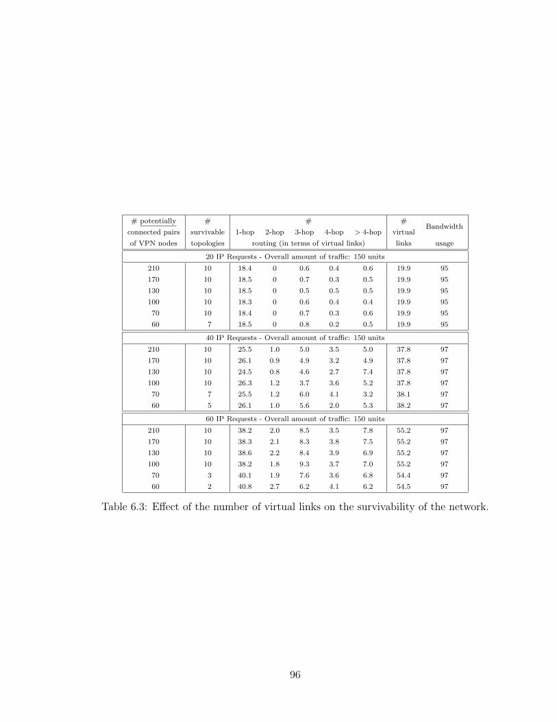
# potentially # # #Bandwidth
connected pairs survivable 1-hop 2-hop 3-hop 4-hop > 4-hop virtual
of VPN nodes topologies routing (in terms of virtual links) links usage
20 IP Requests - Overall amount of traffic: 150 units
210 10 18.4 0 0.6 0.4 0.6 19.9 95
170 10 18.5 0 0.7 0.3 0.5 19.9 95
130 10 18.5 0 0.5 0.5 0.5 19.9 95
100 10 18.3 0 0.6 0.4 0.4 19.9 95
70 10 18.4 0 0.7 0.3 0.6 19.9 95
60 7 18.5 0 0.8 0.2 0.5 19.9 95
40 IP Requests - Overall amount of traffic: 150 units
210 10 25.5 1.0 5.0 3.5 5.0 37.8 97
170 10 26.1 0.9 4.9 3.2 4.9 37.8 97
130 10 24.5 0.8 4.6 2.7 7.4 37.8 97
100 10 26.3 1.2 3.7 3.6 5.2 37.8 97
70 7 25.5 1.2 6.0 4.1 3.2 38.1 97
60 5 26.1 1.0 5.6 2.0 5.3 38.2 97
60 IP Requests - Overall amount of traffic: 150 units
210 10 38.2 2.0 8.5 3.5 7.8 55.2 97
170 10 38.3 2.1 8.3 3.8 7.5 55.2 97
130 10 38.6 2.2 8.4 3.9 6.9 55.2 97
100 10 38.2 1.8 9.3 3.7 7.0 55.2 97
70 3 40.1 1.9 7.6 3.6 6.8 54.4 97
60 2 40.8 2.7 6.2 4.1 6.2 54.5 97
Table 6.3: Effect of the number of virtual links on the survivability of the network.
96

#p
ote n
tial
lyM
ult
i-hop
routi
ng
Sin
gle-
hop
routi
ng
Diff
eren
ce
connec
ted
pai
rs#
surv
ivab
legap
##
connec
ted
#su
rviv
able
gap
##
connec
ted
inth
e#
ofto
pol
ogie
sligh
tpat
hs
vir
tual
top
olog
ies
ligh
tpat
hs
pai
rsof
ligh
tpat
hs
VP
Nnodes
VP
Nnodes
VP
Nnodes
(%)
20IP
Req
ues
ts-
Ove
rall
amou
nt
oftr
affic:
150
unit
s
210
105.
515
7.6
20.0
105.
616
2.5
20.0
3.1
170
105.
215
6.9
20.0
105.
316
2.8
20.0
3.6
130
105.
115
7.9
20.0
105.
816
2.9
20.0
3.2
100
105.
315
8.4
20.0
105.
516
3.3
20.0
3.1
40IP
Req
ues
ts-
Ove
rall
amou
nt
oftr
affic:
150
unit
s
210
106.
316
0.3
37.8
1011
.216
7.8
40.0
4.7
170
106.
516
1.5
37.8
1011
.716
8.6
40.0
4.4
130
107.
016
1.4
37.8
1011
.916
9.0
40.0
4.5
100
107.
116
1.7
37.8
1012
.316
9.3
40.0
4.5
60IP
Req
ues
ts-
Ove
rall
amou
nt
oftr
affic:
150
unit
s
210
107.
216
1.3
55.2
1017
.817
7.6
60.0
10.1
170
107.
216
1.7
55.2
1018
.017
8.2
60.0
10.2
130
108.
116
3.8
55.2
1019
.117
9.9
60.0
9.8
100
107.
916
3.2
55.2
1018
.217
8.5
60.0
9.4
Tab
le6.
4:M
ult
i-hop
routi
ng
vers
us
singl
e-hop
routi
ng.
97

We can also see that, most of the demands are single hop routing, which is a
consequence of the objective of minimizing the number of lightpaths. The very small
number of 2-hop routing can be explained by the fact that the probability of having
3 IP demands defining a triangle, with granularities such that one of the IP requests
can be routed on a two hop route, with each hop being associated with the two other
requests, is very small.
The number of hops increases when the number of IP requests increases. Indeed,
the percentage of multi-hop virtual routes increases from 7% in the case of 20 IP
requests to 10% for 40 IP requests and to 35% for 60 IP requests. This is easily
explained by the fact that, when the number of IP requests increases, it is easier for
an IP request to be routed using other IP request routes.
Since a large number of routes are single hop routes, the number of virtual links
is fairly close to the number of IP requests as can be seen in the penultimate column.
Indeed, we observe a slight increase of the number of virtual links when the percentage
of single hop routes increases.
Lastly, in the last column, we report the bandwidth usage. It is computed as
the ratio of the sum, over all physical links, of the used bandwidth, over the spare
bandwidth (considering only the activated wavelengths). We can see that the band-
width usage is increased when we increase the number of IP requests. Indeed, when
the number of IP requests increases, the routing is more efficient leading to a better
bandwidth usage.
6.6.6 Multi-hop routing versus single hop routing
As mentioned in Section 6.4, the proposed optimization model can also be used to
impose single hop routing by setting the virtual network flow variables as follow:
φsd`′:src(`′)=s,dst(`′)=d = ∆sd. This amounts to forcing the virtual links connecting the
two endpoints of an IP request to carry the whole traffic of that demand. Results
are shown in Table 6.4. Therein, we observe that there is a slightly smaller number
of lightpaths when switching from single-hop routing to multi-hop routing. This is a
consequence of the results observed in Table 6.3 with respect to the small number of
virtual routes with multi hops.
98

6.7 Conclusions
The first contribution of this study is a highly scalable model to design survivable
VPN topologies over a service provider network. The investigation of the impact of
allowing multi-hop virtual routes for IP traffic in a resilient virtual network leads
to the conclusion that, when the virtual topology is resilient, most IP requests are
routed on a single hop route. However, there are cases where multi-hop routing leads
to up to 10% bandwidth savings.
99

Chapter 7
Resilience options for provisioning
anycast cloud services with virtual
optical networks
7.1 Introduction
Today, cloud computing plays a crucial role in cost-efficiently supporting almost any
application domain, an evolution which heavily relies on the advances in (optical)
networking [44]. A core concept in the cloud domain, and one that has recently also
been applied in the networking field itself, is that of virtualization. This boils down
to providing an extra level of abstraction, such that the same underlying physical in-
frastructure can be used by different entities, each in a virtually isolated environment
(e.g., a virtual machine in a data center). Similarly, physical networking infrastructure
(i.e., fibers and switching equipment) can thus be shared by various virtual network
operators (VNOs) [30]. The logical partition under the control of the VNO amounts
to a virtual network topology, denoted as virtual network (VNet), operated in isola-
tion from other VNOs. The physical network and data center infrastructures are then
managed by typically different entities, the physical infrastructure providers (PIPs).
(In practice VNOs and PIPs could indeed be different companies.)
We will study how to resiliently provision VNets for cloud services: requests to be
served by a VNO need to be allocated server capacity at a certain data center (DC)
– whose physical location, i.e., mapping to a particular PIP’s infrastructure, can be
100

decided by the VNO – and obviously network connectivity from the VNO’s customer
to their assigned DC(s). We focus on a planning problem addressing multiple VNets
simultaneously. In this paper, we propose new models for end-to-end cloud services
with different quality in terms of recovery times and availabilities, under both network
and DC failures. Our contributions are:
• Compared to earlier work by Barla et al. [15, 8, 9] (see Section 7.2), our resilience
approach explicitly includes the required network connectivity and associated
bandwidth between a primary and backup data center.
• We introduce a comprehensive qualitative overview of the various resilience
options in choosing the aforementioned synchronization path (beyond the single
simple choice adopted in our initial short paper [22] on this topic).
• We provide full model details for four resilience approaches (not covered in [22]),
and a large scale case study (beyond the small problem instances covered by
e.g., Barla et al. [15]) for two of them on a US topology.
The remainder of this paper is structured as follows: Section 7.2 outlines related
work. The two fundamental resilience strategies (VNO-resilience and PIP-resilience)
are summarized in Section 7.3, while Section 7.4 further details the various choices in
the quality of the protection. The models, adopting a column generation approach,
are detailed in the subsequent Section 7.5 and Section 7.5.5. Our case study results
are presented in Section 7.6, and we conclude in the final Section 7.7.
7.2 Related work
The focus of this work is the joint planning of multiple VNets, as introduced by
Barla et al. in [15], which explains the two major resilience strategies (VNO- vs
PIP-resilience) and focuses on delay minimization. Optimization of resource cost
is treated by the same authors in [9], but there they do not account for resources
for synchronization between primary and secondary data centers (DC). Furthermore,
those authors also point out that other work treats optimization of (i) routing cloud
service requests and (ii) mapping a VNet to the physical infrastructure separately. In
the problem of survivable VNet embedding, [81] and [133] consider that the VNet is
already designed and given, while in [20, 68], the authors build the most bandwidth
101

efficient resilient VNet, under unicast traffic assumptions and using either single or
multiple hop routing of requests in the virtual network. In proposing solutions for
optimal server selection, as well as physical layer routing of anycast services for intra-
and inter-DC networks, the resilience of the resulting virtual layer design is not con-
sidered by [75, 3]. It is important to note that we deal with a planning problem,
jointly deciding on multiple VNets, and not an online VNet mapping that maps one
VNet at a time (as in, e.g., [131]).
The current paper explicitly addresses solving the resilient VNet design and map-
ping problem with simultaneous routing of the requests. This is undeniably related
to the general problem of dimensioning optical clouds/grids: how to find the (min-
imal) amount of network and DC resources, to meet a set of given cloud service
requests? A major complexity arises from the anycast principle: we have flexibil-
ity in choosing a DC among a given set of possible locations. Hence, the classical
notion of a (source,destination)-based traffic matrix disappears [46]. While we previ-
ously developed scalable methods to solve the resilient anycast dimensioning problem
[112, 44, 43], that work did not consider synchronization between distinct working
and backup data center locations (as opposed to the current work). We believe this
is the first work to discuss this in depth: previously we only sketched initial ideas in
[22].
Having synchronization paths with parameter δ (0 ≤ δ ≤ 1, representing the
fraction bandwidth that is required for synchronization between the primary and the
backup data center) make our models more realistic and flexible. We can apply the
models to different kinds of network services. For example, a video streaming service
does not require a large synchronization bandwidth between primary and backup
data center because the main information that needs to be synchronized between
two data centers would be the current playing position. On the other hand, an
online backup service would need as much synchronization bandwidth as the working
bandwidth to keep the transition between two data centers smooth in case of failures.
In this chapter, we study the effect of synchronization bandwidth on total bandwidth
requirement by choosing two extreme values of δ, being 0.1 and 0.9 respectively.
102

7.3 VNO- vs PIP-resilience
Cloud service requests that we consider a VNO to support, are assumed to have a
given origin s (i.e., the location of customer of the VNO), and need to be served
at a data center d (where server capacity should be allocated) and requires network
connectivity between the (s, d) pair. Assuming anycast, d can be chosen out of a set
of given locations (i.e., where the VNO can rely on a PIP’s infrastructure). We will
design the VNet such that requests can survive single failures, which can each affect
either the physical network or data center infrastructure. We will now discuss the
two fundamental options in doing so: VNO-resilience and PIP-resilience. They are
illustrated in Figure 7.1, where both approaches rely on two disjoint DCs (d1 and
d2) to protect against data center failures. Further, we assume there is an automatic
switch-back to the original network path or DC once a fault is repaired, and therefore
will allow reusing the same network/DC capacity to protect against other failures:
backup capacity is shared. In the VNO-resilience model, 1:1 protection routing is
provided in the VNet for network failures, where the working and protection paths
of a service have to be physically link/node disjoint: the working path w routes the
services towards the primary DC, the protection path b towards the backup DC, and
w and b will be disjoint in their physical layer mapping. In addition, one (or two,
see Section 7.4) synchronization paths s are established in order to handle migration
and failure routing requirements when a DC failure occurs: services then need to be
rerouted from the primary d1 to the backup DC d2. Thus, the resulting VNet for the
request from source s comprises three links, mapped to resp. the physical w, b and
s paths. Note that both w and b need to carry the full traffic (but b only when w
or d1 are affected by a failure), but s possibly only a fraction thereof, only to keep
the state at the backup location d2 synchronized with that of d1 to allow smooth
handover upon d1 failure.
In PIP-resilience, services are routed on single paths in the VNet layer, where each
virtual link is mapped on two link/node disjoint physical paths in the physical layer.
Thus, there will be a single virtual link connecting the source s to the primary data
center d1, which in the physical layer will be supported by the two disjoint paths w
and b. In addition, to cater for DC failures, a second location d2 will be chosen, and
connectivity between d1 and d2 will be provided along the physical path s. Thus,
the VNet will comprise only two virtual links. In terms of capacity, it is important
103

VNO
Working
Backup
PIP
(a) VNO-resilience.
VNO
Working
Backup
PIP
(b) PIP-resilience.
Figure 7.1: Two resilience schemes.
104

to note that under PIP-resilience the s path needs to carry not just synchronization
traffic but also the full traffic bandwidth (hence the additional red line in Figure 7.1)
in case of d1 failure.
7.4 Quality of the resilience schemes
From the discussion above, it is clear that the w and b paths need to be disjoint (for
both VNO- and PIP-resilience). However, depending on the recovery time require-
ments, we can have different disjointness requirements for s or even choose to have
two disjoint synchronization paths s and s′, as argued below. For the sake of clarity,
we will discuss in detail the various failure scenarios and how they are dealt with in
the two fundamental resilience schemes.
7.4.1 VNO-resilience
Let us first consider a single link failure, say of link `, and then the single DC failure:
(i) If ` ∈ w fails, then the request will be rerouted to the backup data center d2,
using the backup path b (which is disjoint from w, thus ` /∈ b). If it happens that
` ∈ s ∩w, then it means that as long as the failure is not restored, the primary data
center d1 can not be kept in sync with the now operational d2. Thus, right after
the repair of `, the primary d1 will have stale state, and hence switching back to d1
will either suffer from this stale state or need to wait some extra time to receive the
requests again. The remedy is of course to enforce w ∩ s = ∅. (Yet, note that the
same problem of a non-synchronized primary d1 clearly also occurs after the repair
of a d1 that failed itself.)
(ii) If ` ∈ s \ w fails, this does not immediately pose a problem. Yet, if shortly
after `’s repair the working path w fails, the switchover to the backup d2 (via path b)
will suffer from stale state since the failing s will have interrupted the synchronization
between primary and backup DCs. This can only be remedied by providing a second
synchronization path s′ disjoint from s.
(iii) If ` ∈ b fails, again no immediate problem arises (since this means that w
will be operational, given w∩b = ∅). However, if ` ∈ s∩b and shortly after `’s repair
the primary path w (or d1) fails – meaning that now b will be followed towards d2
– the secondary data center d2 might not be fully sync’ed yet. Clearly, this can be
105

remedied by choosing b ∩ s = ∅. Yet, essentially the problem is exactly the same as
for case (ii), which obviously remains, even if we take s ∩ b = ∅. (iv) If the primary
DC at d1 fails, the requests will be rerouted to the backup d2 via the b path. Clearly,
the failing d1 cannot be kept in sync with the now operational backup d2. Thus, we
might need to wait some time after d1’s repair to switch back requests via w. Any
failure that would occur shortly after d1’s repair and which would prevent services
to remain being served at d2 clearly could imply service degradation because of the
unsync’ed d1: (1) failure of s, (2) failure of b, or (3) failure of d2. This can however
not be remedied without extra DC resources or extra paths.
7.4.2 PIP-resilience
(i) If ` ∈ w fails, requests will keep being served at primary d1, but now follow
the b path to get there. If ` ∈ s ∩ w, then it means the secondary DC d2 will
not be synchronized as long as ` is not repaired: if `’s repair is followed closely by
a subsequent failure of the primary DC d1, then d2 will not be fully sync’ed yet,
potentially resulting in temporary service degradation. This can be easily remedied
by choosing s ∩w = ∅.(ii) If ` ∈ s \ w fails, it means that d2 is no longer reachable and remains un-
synchronized. As in the VNO-resilience case, the only remedy is a second, disjoint,
synchronization path s′.
(iii) If ` ∈ b fails, this poses no immediate problem. Yet, if ` ∈ s ∩ b, and shortly
after `’s repair the primary data center d1 fails, the backup d2 will not be fully sync’ed
yet. A possible remedy is choosing s∩b = ∅, but again, the same problem still occurs
under failure of s alone (case (ii)).
(iv) If the primary DC at d1 fails, traffic is deflected to d2 (using the w+ s route).
Obviously, during its failure, d1 remains unsynchronized with the now operational d2.
This means we might have to wait for this synchronization to be completed (via s)
before switching back to a repaired d1. Clearly, a subsequent failure of s will obstruct
that. This can be remedied by a second synchronization path s′, disjoint from s. Yet,
as in the VNO case, the same problem of switch-back to a non-sync’ed d1 can occur
if the repair of d1 is followed by a failing d2.
106

7.4.3 Resilience quality options
To wrap up the previous discussion, if we choose s∩w = ∅, this guarantees a prompt
switchback to the primary d1 in the VNO-resilience case upon clearance of a w failure.
For the PIP-resilience case, it helps smooth switching to the secondary DC upon a
primary DC failure following a repaired w (even though the problem remains for a
cleared s failure followed by a primary DC failure). The benefit of choosing s∩ b = ∅seems limited, since the problems stemming from joint failure of b and s are largely
the same as those stemming from failing just s.
The models discussed in the next Section 7.5 will cover these cases, starting with
just the disjoint w and b conditions, and indicating what constraints to add to ensure
the optional disjointness for s (with w and possibly b).
To ensure continuous synchronization between both data centers, and hence quick
recovery and switchback times upon repairs, one can opt for protecting the synchro-
nization path s by a failure disjoint s′. The corresponding model will be described in
Section 7.5.5.
7.5 Models for a single synchronization path
We will adopt a column generation (CG) approach, as this tends to be a highly
scalable solution methodology (e.g., its application in [112, 43]). That means that
we will divide the model into a Restricted Master Problem (RMP) and a Pricing
Problem (PP). The RMP will take as input a set of given configurations (of w, b
and s paths, see further), and decide which ones to use to achieve minimal cost. The
PP will be responsible for finding such suitable configurations. PP and RMP will
be solved alternately until the optimality condition (no more a configuration with a
negative reduced cost) is satisfied. An integer solution is obtained by solving the last
generated RMP, see the flowchart in Figure 7.2. Scalability is achieved because this
set of PP configurations will be only a fraction of all possible ones. For details on
column generation method, we refer to, e.g., [33].
We focus on a core network, comprising optical links and cross-connects as well
as data centers, that will be modeled by an undirected graph G = (V, L) where V
is the node set (indexed by v) and L is the link set (indexed by `), for which ω(v)
denotes the set of links adjacent to v. Further, the set of data center (DC) nodes will
107

Next Request
Solve ILP of Restricted Master Problem
Add improving configuration
Added columns (configurations)
Dual Values
Optimal LP solution
Restricted Master Problem
(Minimization)
Selection of the best configurations
Found config. w/ negative reduced
cost?
Add improving configuration
Dual DualValues
Master Problem (Minimization)
Selection of the best configurations
Found cw/ negative
cos
Solve pricing (min.) problem to find configuration
(associated w/ request) that has
negative reduced cost
Yes
est
No
Pricing problem
Start w/ first request
ILP ε-optimal solution
Yes
No more requests
Figure 7.2: Flowchart of the CG ILP approach.
be denoted as Vdst ⊆ V , with ndst = |Vdst| the number of DC nodes. Note that
in our setting, a single DC node v ∈ Vdst represents the whole of all real-world data
centers that are connected to the same core network node (i.e., an OXC).
Traffic is defined by the number of services (demands), originating from a set of
source/service nodes Vsrc ⊆ V , with generic index vsrc. Let D be the set of services,
indexed by d. Each service d is characterized by its bandwidth requirement Δd, its
source (or origin) vd, and δd (with 0 ≤ δd ≤ 1), representing the fraction of Δd that
is required for synchronization between the primary and the backup data center.
7.5.1 Master problem: WB-VNO-resilience
In our CG approach, a configuration is associated with a source node (vs) where
some services are requested. Let C be the overall set of configurations: C =⋃
v∈VsCv,
where Cv is the set of configurations associated with source node v ∈ Vs. We define
a configuration c ∈ Cv by: (i) a set of 3 paths, one primary path pw originating at vs
towards a primary data center DCw, one backup path pb originating at vs towards a
primary data center DCb, and one synchronization paths (ps) between the primary
108

and the backup data center, as well as (ii) the services routed and protected by this
set of 3 routes. We will protect against single link failures as well as single data center
failures. (Extension to generic failures modeled as shared risk groups is fairly trivial,
e.g., using a similar approach as [43].)
More formally, a configuration is characterized by the following given parameters1:
ϕw`,c = 1 if link ` is used by the working path of configuration c, 0 otherwise;
ϕb`,c = 1 if link ` is used by the backup path of configuration c, 0 otherwise;
ϕs`,c = 1 if link ` is used by the synchronization path of c between the primary data
center and the backup data center, 0 otherwise;
awv,c = 1 if node v is selected as the primary data center, 0 otherwise;
ab,cv = 1 if node v is selected as the backup data center, 0 otherwise.
The master problem will determine which configurations to use, using integer
decision variables zc. (0 if configuration c is not used). For each link `, let βw` be the
working bandwidth on `, and βb` the backup bandwidth on `. The objective function
is to minimize the overall (working + backup) bandwidth requirements, where ‖`‖denotes the length of link `:
min∑
`∈Lphy
(βw` + βb`
)· ‖`‖ , (79)
subject to: ∑c∈Cd
zc ≥ 1 d ∈ D (80)
∑c∈C
∆dc
(ϕw`,c + δd ϕ
s`,c
)zc = βw` ` ∈ L (81)
∑c∈C
∆dc ϕw`′,c ϕ
b`,c zc ≤ βb` `′ ∈ L, ` ∈ L \ {`′} (82)∑
c∈C
∆dc awv,c ϕ
b`,c zc ≤ βb` v ∈ Vdst, ` ∈ L (83)
1From the master problem’s perspective, these are indeed given parameters. However, in thepricing problem they will become decision variables.
109

zc ∈ {0, 1} c ∈ C (84)
βw` , βb` ∈ IR ` ∈ L. (85)
Constraints (80) are the demand constraints, and ensure that each service k is
granted. Constraints (81) compute the overall bandwidth requirements on link ` under
failure-free conditions: this is the sum of the working path (w) and synchronization
path (s) bandwidths, where the latter only is a fraction δd of the former. Constraints
(82) ensure sufficient backup bandwidth requirements on link ` to cover a failure of
any other link `′. Constraints (83) guarantee sufficient backup bandwidth ` to handle
any data center failure.
Note that in our experiments, we will not consider any network capacity con-
straints. However, should one want to pose capacity limits on the links, this can be
accommodated by adding the following constraints (using BW` to denote the capacity
of link `):
βw` + βb` ≤ BW` ` ∈ L. (86)
7.5.2 Master problem: WB-PIP-resilience
For PIP-resilience, we need to replace constraints (83) with (87). Remark that s will
need to support the full request bandwidth when a node failure occurs at the primary
data center (but it can be shared among different failure cases):∑c∈C
∆dc awv,c ϕ
s`,c zc ≤ βb` v ∈ Vdst, ` ∈ L. (87)
Note that the synchronization bandwidth on the s path will be reserved on top of that
(see (81) in the master problem). Since the backup capacity on s is only required when
the primary DC fails, we then cannot synchronize and hence one could argue that we
should actually add a factor 1− δd in (87). Yet, upon restoration of the primary DC
failure, we will need to synchronize it and thus do need the synchronization bandwidth
in addition to the full traffic bandwidth along the path s.
7.5.3 Pricing problem: WB-VNO-resilience
Recall that the pricing problem (PP) will determine useful configurations, i.e., routes
for w, b and s paths. Each PP is written for a given source node vs and for a given set
110

of requests originating there. The given parameters ∆d and δd retain their definition
for a request d as in the RMP.
The sets of variables are as follows:
pw` = 1 if link ` is used by the working path of the configuration under construction,
0 otherwise;
pb` = 1 if link ` is used by the backup path of the configuration under construction,
0 otherwise;
ps` = 1 if link ` is used by the synchronization path of the configuration under
construction between the primary data center and the backup data center, 0
otherwise;
awv = 1 if node v is selected as a data center location by the working path in the
configuration under construction, 0 otherwise;
abv = 1 if node v is selected as a data center location by the backup path in the
configuration under construction, 0 otherwise;
dwv = 1 if node v is on the working path in the configuration under construction, 0
otherwise;
dbv = 1 if node v is on the backup path in the configuration under construction, 0
otherwise;
dsv = 1 if node v is on the synchronization path between the primary data center and
the backup data center in the configuration under construction, 0 otherwise.
The objective of the PP is to minimize the reduced cost as obtained from the
RMP, defined as:
cost = 0−∑
`∈Lphy
u(81)` ∆dc
(ϕw`,c + δd ϕ
s`,c
)− ud
−∑`∈L
∑`′∈L\{`}
u(82)``′ ∆dϕ
w` ϕb`′ −
∑v∈Vdst
∑`∈Lphy
u(83)v` ∆da
wv p
b` (88)
where u(81), u(80)v , u
(82)``′F , u
(83)v` are the values of the dual variables associated with
constraints (81), (80), (82), (83), respectively. (Note that the first explicit 0 term
stems from the RMP objective, which does not contain the configuration variable zc.)
111

The path and data center variables have to obey:
∑`∈ω(v)
pw` =
1− awv if v = vs
2 dwv − awv otherwisev ∈ V (89)
∑`∈ω(v)
pb` =
1− abv if v = vs
2 dbv − abv otherwisev ∈ V (90)
∑`∈in(v)
ϕs` = 2 dsv − awv − abv v ∈ V (91)
ϕw` + ϕb` ≤ 1 ` ∈ L (92)∑v∈Vdst
awv = 1 ;∑
v∈Vdst
abv = 1 ;∑
v/∈Vdst
awv + abv = 0 (93)
awv + abv ≤ 1 v ∈ Vdst (94)
awv , abv ∈ {0, 1} v ∈ V (95)
ϕw` , ϕb` , ϕ
s` ∈ {0, 1} ` ∈ L. (96)
Constraints (89)–(91) are the conventional flow constraints for working, backup and
synchronization paths. Constraints (92) force pw and pb to be disjoint2. Constraints
(93) ensure that each configuration has exactly one primary and one back up data
center, while constraints (94) coerce them to be different. Constraints (95)–(96) define
the domains of the variables.
7.5.4 Pricing problem: WB-PIP-resilience
The objective of the PP for the PIP-resilience case is:
cost = 0−∑
`∈Lphy
u(81)` ∆dc
(ϕw`,c + δd ϕ
s`,c
)− ud
−∑`∈L
∑`′∈L\{`}
u(82)``′ ∆dp
w` p
b`′ −
∑v∈Vdst
∑`∈L
u(87)v` ∆da
wv p
s` . (97)
Further, the flow constraints need to be modified in order to enforce both working
and backup paths to connect to the primary data center. The constraints (90) are
2This ensures protection against single link failures. For a more extensive protection againstmultiple simultaneous failures, one can model these as shared risk groups (SRGs) and use a similarapproach as in [43].
112

replaced by (98):
∑`∈ω(v)
pb` =
1− abv if v = vs
2dbv − awv otherwisev ∈ V. (98)
7.5.5 Improved QoS strategies
Disjointness between W and S
As discussed in Section 7.4, by enforcing the disjointness between w and s we can
reduce the transition time when having two consecutive failures, first on the working
path then on the backup path (for VNO-resilience) or primary data center (for PIP-
resilience) (i) for the VNO-resilience case to switch back to the primary data center
after clearance of a w failure, and (ii) for the PIP-resilience case to switch to the
secondary data after two consecutive failures, first on w, then of the primary data
center. This can be realized by adding constraints (99) to the pricing problem:
ϕw` + ϕs` ≤ 1 ` ∈ L. (99)
Accordingly, should one want to enforce disjointness between s and b, similar
constraints can be added (replacing ϕw` with ϕb` in (99)).
Having two synchronization paths
As motivated in Section 7.4, one could opt to implement two synchronization paths s
and s′ connecting the primary and backup data center. We need to replace constraints
(82) with constraints (100) as the synchronization path also has backup capacity. The
objective of the pricing is also needed to be changed accordingly.∑c∈C
(∆dc ϕ
w`,c ϕ
b`′,c + δd ∆dc ϕ
s`,c ϕ
s′`′,c
)zc ≤ βb`′
` ∈ L, `′ ∈ L \ {`} (100)
For the corresponding pricing problems, we need to add flow constraints for s′ and
disjointness constraints between s and s′:∑`∈ω(v)
ϕs′
` = 2ds′
v − awv − abv v ∈ V (101)
113

Scattered DCs
δ = 0.1
Scattered DCs
δ = 0.9
Paired DCs
δ = 0.1
Paired DCs
δ = 0.9
●●
● ●
● ●●
●●
●●
●●
●
●●
●● ●
●●
●●
●●
●●
●
●●
●●
●●
●
●●
●●
●●
●
● ●●
●● ●
●
● ●●
●●
●●
●●
●● ●
● ●
●●
● ●● ●
●
●●
●● ●
●●
●●
●●
● ●●
●●
●●
●●
●
●●
●● ● ●
●
●● ●
● ●●
●
●●
●● ●
● ●
0
50000
100000
150000
200000
0
50000
100000
150000
200000
{W,B
} disjoint{W
,B} and {W
,S} disjoint
10 20 30 40 10 20 30 40 10 20 30 40 10 20 30 40Load (normalized bandwidth unit)
Cos
t (no
rmal
ized
ban
dwid
th×
km)
ResiliencePIP
VNO
Bandwidth
●
Total
Backup
Working
Sync
Figure 7.3: Experiments on the US topology, for {w, b} disjointness (top), both {w, b}and {w, s} disjointness (middle), and two synchronization paths (bottom).
ϕs` + ϕs′
` ≤ 1 ` ∈ L. (102)
Note that, in this protection scheme, while we have two synchronization paths,
only one path is needed to be functional in normal situation (i.e., no failures). The
other path is used when there is a failure on the first synchronization path. Therefore
the bandwidth for the second path can be shared.
7.6 Numerical results
7.6.1 Data sets
We first run experiments on the 24-node US nationwide backbone network shown in
Figure 7.4 with 4 data centers. The network has 43 non-directional links, labeled with
their lengths in km. The bandwidth requirement for each service request is generated
randomly with uniform distribution between 0 and 1 normalized bandwidth units.
We generate uniform traffic, i.e., the source node of a request is chosen randomly,
and vary the total requested bandwidth (i.e., the total load) from 10 to 40 units (the
number of generated requests varied from 22 to 83). As per the CG model, each
request is individually provisioned: requests originating from the same source node
114
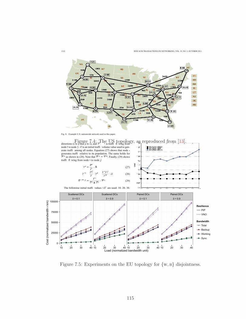
2) Numerical Results:
Figure 7.4: The US topology, as reproduced from [13].
δ δ δ δ
●●
●●
●●
●
●●
●●
●●
●
●●
●●
●●
●
●●
●●
●●
●
●●
●
●
●
●
●
●
●●
●
●
●
●
●●
●
●
●
●
●
●
●
●●
●
●
●
×
●
Figure 7.5: Experiments on the EU topology for {w, b} disjointness.
115

Dublin
Glasgow
London
Paris
Bordeaux
Madrid
Barcelona
Lyon Milan
Rome
Zurich
Strasbourg
FrankfurtBrussels
Amsterdam
Hamburg
Berlin
MunichPrague
ViennaBudapest
Zagreb Belgrade
Warsaw
Stockholm
Copenhagen
Oslo
Athens
Dublin
Glasgow
London
Paris
Bordeaux
Madrid
Barcelona
Lyon Milan
Rome
Zurich
Strasbourg
FrankfurtBrussels
Amsterdam
Hamburg
Berlin
MunichPrague
ViennaBudapest
Zagreb Belgrade
Warsaw
Stockholm
Copenhagen
Oslo
Athens
Figure 7.6: Experiments on the NobelEU network with all possible data center loca-
tions indicated with a star symbol.
are not forced to follow the same paths towards the same data centers.
To study the effect of DCs location, we consider two sets of DC locations. In the
first set, DCs are fairly uniformly scattered over the geographical region: {WY(6),
AZ(8), IL(11), AL(18)}. In the second set, DCs are selected in paired locations:
{CA(3), UT(7), KY(16), NC(22)}. (A motivation for using paired locations could be
to aim to have similar path lengths, and hence latencies, to both the primary and
backup data centers3.) For each DC constellation, we carry out the experiment for
two synchronization parameter settings: δ = 0.1 and δ = 0.9.
In the first set of the experiments, we choose the 24-node US nationwide back-
bone network. This network topology is more grid-like. To study the effect of network
topologies over the performance of the two models, we do the second set of experi-
ments on NobelEU network which has 28 nodes, 82 directed links (see Figure 7.6).
Similarly, we do the experiment on two set of DCs: The first set of DCs consists of
3We verified that for the chosen paired DC locations, the majority of the source nodes indeedhas one of the pairs as two closest, path-disjoint, DCs among the four given in total.
116

Lyon, Berlin, London, and Vienna, which are scattered rather evenly across the cen-
tral network nodes. The second set of DCs has two pairs of neighboring DC locations:
Amsterdam, Hamburg, Lyon, and Zurich.
7.6.2 Effect of DC locations and synchronization bandwidth
We expect VNO-resilience to outperform PIP-resilience in all settings, since under
VNO-resilience we have more flexibility to choose the backup paths than for PIP-
resilience (indeed, the physical routing as obtained in the latter case is always also
allowed in VNO-resilience). This is confirmed by our results shown in Figure 7.3,
which we now discuss in detail.
First of all, going from scattered to paired DC locations, we find that the total
bandwidth cost is reduced by roughly 30% (for the same δ and resilience scheme).
This can be explained by the fact that paired DCs enable more sharing, since the
backup paths go to 2 regions (east and west) instead of 4, and the synchronization
paths are shorter.
Intuitively, we expect the paired DC configuration to have lower cost differences
between VNO- and PIP-resilience. Indeed, VNO-resilience’s potential advantage
mainly stems from shorter backup route options avoiding the inter-DC path, yet
this path is quite short in the paired DC case and thus does not amount to a heavy
penalty. Our results confirm this, and the cost advantage VNO-resilience even is neg-
ligible in the δ = 0.9 case: for high δ the synchronization bandwidth becomes more
dominant (thus limiting VNO’s gain in terms of lower backup bandwidth).
Moving from scattered DCs experiment to paired DCs experiment, the difference
between two models decreases which is intuitively correct because the differences
between backup paths of the two models decrease. Obviously, overall cost for both
VNO- and PIP-resilience and both DC settings does increase for higher δ.
Clearly, the overall bandwidth cost increases for higher synchronization bandwidth
(i.e., higher δ). The relative cost advantage of VNO-resilience over PIP-resilience
however diminishes, since. In the case when δ = 0.9 and DCs are located in pair, the
results of the two models are almost identical.
117

7.6.3 Effect of disjointness of W and S
In our experiments, the penalty for adding the disjointness between w and s is very
small at less than 5%. It is likely that in most cases, W and S are already link-
disjoint which is also intuitively understandable. This suggests that we can improve
the quality of the resilience (in terms of recovery times, see Section 7.4) by enforcing
the disjointness between w and s, and only pay an almost negligible extra bandwidth
cost.
7.6.4 Effect of having two synchronization paths
This protection scheme, as discussed in the previous section, have a shorter recovery
time than two previous schemes. Because the bandwidth for the second synchroniza-
tion path can be shared among other synchronization paths or backup paths, the cost
of having two synchronization paths is only about 10% higher than having W and S
disjoint.
7.6.5 Effect of the network topology
In the US network experiment, moving from scattered DCs experiment to paired DCs
experiment, the difference between two models decreases. Intuitively, this is because
in the pair scenario, the primary DC and the backup DCs tend to be in pair to
minimize the cost, therefor the differences between backup paths of the two models
decrease. This can be seen in Figure 7.7. When δ = 0.9, because of the important of
the synchronization path, this trend is much stronger, even in the case of scattered
DCs.
However, in the EU network experiment, we do not see the behaviors of two mod-
els changes when moving from scattered DCs experiment to paired DCs experiment
as shown in Figure 7.5. This is because the DCs do not go in pair as in the US
experiment. This can be confirmed in Figure 7.7 where the distribution of primary
DCs and backup DCs are plotted. This can be explained by the fact that the topol-
ogy of EU network is less grid-like which create some long detour backup paths and
consequently making the difference between the pair DCs and the scatter DCs less
clear. Let us take an example with a request from Athens, as the working path is
usually the shortest path, it goes to Zurich via Rome and Milan. The backup path
118

Figure 7.7: Distribution of primary and backup DCs on US network.
for PIP would go through Belgrade, Zagreb, Vienna, Munich, Frankfurt, Strasbourg,
to Zurich. The backup path for VNO will not go to the same pair (i.e., to Lyon) as
it involves even a longer path. Similar situations would apply to request from other
rear nodes.
The particularity of the network topology does effect the quality of the resilience
of the two models, it is important to choose the location of the DCs when the topology
is less grid-like.
7.7 Conclusions
We have carefully outlined the various options in providing resilient virtual networks
for cloud services, thus under an anycast traffic scenario: we only assumed the traf-
fic sources to be given, while destinations can be chosen among a set of given data
center (DC) locations. We considered a virtualized network environment, where vir-
tual network operators (VNOs, that will provision the cloud service requests) make
use of underlying physical infrastructure offered by physical infrastructure providers
(PIP). We explained the different mappings in a VNO- vs a PIP-resilience scenario,
comprising not just working and backup paths, but also explicitly accounting for
119

Figure 7.8: Distribution of primary and backup DCs on EU network.
the synchronization path (and associated bandwidth cost) between primary and sec-
ondary data centers. We indeed provide resilience against both network and DC
failures. Our thorough discussion of the various failure scenarios revealed disjointness
requirements for that synchronization path that can improve the quality of resilience
in terms of recovery times.
We subsequently detailed scalable models to find routings and DC allocations for
cloud requests, with minimal cost, for the proposed resilience strategies (VNO vs
PIP) and options for the synchronization path (one or two disjoint ones). Our results
show that the intuitively expected advantage of VNO-resilience actually can be quite
limited, when DCs occur in paired configurations (which may be desirable to obtain
similar latencies towards both primary and backup DC). Moreover, if the synchro-
nization bandwidth becomes a substantial fraction of the actual traffic bandwidth,
this relative cost advantage becomes very limited.
120

Chapter 8
Scalable algorithms for QoS-aware
virtual network mapping for cloud
services
8.1 Introduction
Cloud services have become increasingly popular from the customer’s perspective
mainly because of convenience: applications are offered “in the cloud” and thus fa-
cilitate access from anywhere on almost any device. Technically, this clearly relies
on reasonably high bandwidth connectivity. The core network, carrying the aggre-
gated end user traffic in bulk and providing connectivity towards the large scale data
center infrastructures (where the aforementioned services are actually running), is
cost effectively realized by optical network technology: we refer to such networks as
optical clouds (see [45] for a discussion on the applications that have driven this evo-
lution, and the optical network technology challenges). Traditional network design
algorithms, such as the typical routing and wavelength assignment (RWA) strategies,
however cannot be directly applied in the context of optical clouds. Fundamentally,
this is due to two core principles underlying cloud technologies: anycast routing and
virtualization.
Anycast routing refers to the fact that users do not greatly care about the exact
location of the actual servers running the applications they are using. Thus, service
providers have some flexibility in deciding where to serve what requests. From the
121

network perspective, this means that the destination of traffic is not fully specified
in advance. From the network’s perspective, it implies that the destination of traffic
flows is not given a priori. Moreover, clearly the network infrastructure cannot be
treated completely independent from the data center infrastructure capacity (since
terminating traffic needs to be served by the data center resources). The joint dimen-
sioning of network and data center infrastructure to resiliently support cloud services
has been studied, e.g., in [43].
Virtualization implies that physical infrastructure is logically partitioned in dis-
joint virtual resources. On the data center side, this means servers are running mul-
tiple so-called virtual machines (VMs) that have no access to each other’s resources.
Similarly, in recent years the concept of virtualization has also been applied to net-
works [94]: different virtual networks (VNets) can be run by independent virtual
network operators (VNOs) that make use of the same physical network infrastruc-
ture, offered by physical infrastructure providers (PIPs). Both for server and network
virtualization, the rationale is to share the same physical resources (thus reducing
the capital expenditure for hardware), but still to provide isolation (by logically seg-
regating the services over disjoint (virtual) resources).
Here, we study the provisioning of VNets for cloud services both resiliently and
with assurance of quality of service (QoS). Requests need to be served by a VNO,
who thus needs to allocate server capacity at a particular data center (DC), and
provision network connectivity from its customers to their respectively assigned DCs.
The VNO’s logical VNet will be provided through a mapping to physical resources
offered by a PIP. Furthermore, we will ensure the request’s QoS requirements (i.e.,
end-to-end delay between source and destination) are respected, and consider 3 classes
of virtual resources. Our novel contributions are:
• Compared to our earlier works adopting column generation in (e.g., [43, 20])
and precursory work on VNet mapping [9] we (i) account for service QoS dif-
ferentiation, and also (ii) adopt a more detailed/realistic VNO cost model (e.g.,
accounting for virtual node costs).
• Compared to initial work on QoS-aware mapping [12], we (i) consider anycast
instead of unicast demands, (ii) adopt a more realistic delay modeling), and
(iii) present a a truly scalable column generation based formulation instead of
a simple (non-scalable) ILP formulation.
122

• We demonstrate the near-optimality and scalability of our solution on a 28-node
EU topology, thus providing a thorough assessment of the pros and contras of
two resilience options in terms of both (i) VNO setup costs, and (ii) physical
resource utilization.
8.2 Resilient virtual network mapping with QoS
We consider the problem of mapping a given set of cloud requests into a virtual
network design, such that it is resilient against failures of both the network and
data center infrastructure, while respecting the requests’ QoS constraints under all
circumstances. We formalize this as follows: Given:
• The network topology, described by
– Gphy = (V phy, Lphy), the physical network comprising the physical nodes
V phy and interconnecting links Lphy.
– Gvir = (V vir, Lvir), the virtual network with candidate virtual nodes V vir,
as well as candidate virtual links Lvir. There will be a one-to-one mapping
between each virtual node v′ ∈ V vir and a single physical v ∈ V phy (thus
V vir ⊆ V phy), but multiple candidate virtual links will be considered between
the same virtual node pair with mappings to distinct physical paths.
– V dc ⊆ V vir, the set of data center locations.
– The set of all paths π ∈ Π in the physical network corresponding to the mapping
of any virtual link `′ ∈ Lvir.
• The cloud requests d ∈ D, each one characterized by
– A source node srcd ∈ V vir,
– The requested bandwidth ∆bwd ,
– The requested number of virtual machines ∆vmd ,
– The minimal QoS class of the VMs, qd ∈ Q, and
– A maximal end-to-end delay (i.e., between source and chosen DC) of δd.
Find: For each request d ∈ D, a working (w) and backup (b) data center to use, as
well as routes in the virtual network Gvir towards them, such that:
123

• Each request d can always be served, both in failure-free conditions as well as under
any failure scenario,
• The QoS of every request d is respected,
• The total network cost is minimized, and
• The physical network capacity constraints are respected.
Hence, we face a resilient virtual network mapping problem. The failures we will
protect against will be single failures of either a physical link (` ∈ Lphy), or a complete
data center (v ∈ V dc). We will consider two resiliency approaches: VNO-resilience
or PIP-resilience [22, 9]. As sketched in Figure 8.1, in case of VNO-resilience, the
protection is handled by the virtual network operator, and requests are rerouted in
the virtual network both in case of physical network failure and DC failure. On
the other hand, in case of PIP-resilience, a virtual link is mapped resiliently to two
failure-disjoint paths in the physical network1. Thus, only in case of a data center
failure, an explicit reroute to another data center is required (using an unprotected
link). Note however that in reality, the b path will not be exposed to the VNO.
Still, the PIP still has to provision it and it will have associated costs. Hence, from
a modeling perspective, we do represent it in the VNO layer. Note that we do not
consider shared protection: bandwidth will not be reused among protection paths
that are activated under different failure scenarios. Furthermore, we will assume
failure-independent rerouting: for a given request the backup route (and destination)
will be the same regardless of the failure affecting the primary route.
The QoS constraints associated with a request d are first of all the QoS class
of the VMs to be installed, and secondly the end-to-end delay from source node to
destination DC. The latter is the sum of the virtual link and node delays. The delay
of a virtual link depends on the propagation delay (i.e., the physical path length) and
the sum of the delays over the intermediate physical nodes (for which we will use a
fixed value, see Section 8.5). The delay of a virtual node depends on its QoS class:
just as VMs, we assume to have the choice between different virtual node types of a
given class q ∈ Q, each with their associated forwarding delay (δnode,q).
1Remark that this means that in the PIP-resilience case, Lvir may contain multiple parallellinks between the same virtual node pair: defining πpw
`′ resp. πpw`′ as the two paths in the physical
layer, parallel virtual link candidates may share the same πpw`′ , or πpb
`′ , but not both.
124

VNO
Working
VNO
Working
Backup
Backup
VNO-resilience PIP-resilience
PIPPIP
Figure 8.1: Two resilience schemes.
The cost model comprises a data center component (the VMs) and a virtual net-
work provisioning part. The data center cost will be the cost of installing VMs:
costvm,qv : the cost per installed VM of class q at DC v ∈ V dc.
The virtual network cost will be a summation of node and link costs, with a fixed
part independent of the traffic volume crossing it, as well as a bandwidth-dependent
part:
cost setuplink`′ : cost of instantiating candidate virtual link `′ ∈ Lvir as a class
q ∈ Q link. In our experiments, this cost will be dependent on both the class q
and the link length |`′| (see further, Section 8.5).
costlink`′ : cost of using a single unit of bandwidth capacity on a class q virtual link
`.
cost setupnode,qv : cost of instantiating a class q virtual node at v.
costnode,qv : the cost of forwarding a single unit of bandwidth capacity through a
class q virtual node at v ∈ V vir.
The capacity limits of the physical links and virtual nodes are assumed to be given:
caplink` : bandwidth limit on physical link ` ∈ Lphy
capnodev : maximal virtual node capacity at node v ∈ V vir
125

Next Request
Solve ILP of Restricted Master Problem
Add improving configuration
Added columns (configurations)
Dual Values
Optimal LP solution
Restricted Master Problem
(Minimization)
Selection of the best configurations
Found config. w/ negative reduced
cost?
Add improving configuration
DualualDualualValues ue
Master Problem(Minimization)
Selection of the best configurations
Found cw/ negative
cos
Solve pricing (min.) problem to find
configuration (associated w/ request) that has
negative reduced cost
Yes
est
No
Pricing problem
Start w/ first request
ILP -optimal solution
Yes
No more requests
Figure 8.2: Decomposition flow chart.
capvmv : maximal VM capacity that is available in the DC at node v ∈ V dc (which
will in practice depend on the physical server capacity). Note that we assume
that the capacity of a single VM instance depends on its class q only, which we
will denote as capvm,q.
8.3 Column generation model: VNO scheme
We adopt a column generation (CG) approach to obtain a highly scalable model (e.g.,
its application in [112, 43]). The model thus is split into a Restricted Master Problem
(RMP) and a Pricing Problem (PP), as sketched in Figure 8.2. Given a set of given
configurations, the RMP decides which ones to select to achieve minimal cost. For
details on column generation we refer to Section 2.4.2.
8.3.1 Master problem
Parameters and variables
We denote by � a generic physical link and by �′ is a generic virtual link. A config-
uration c is associated with a particular demand dc and is characterized by:
126

– costc, its cost for usage per unit request, which includes the cost for virtual nodes,
links, and VMs;
– pc` = 1 if ` ∈ Lphy belongs to the working or backup path;
– ynode,q,cv = 1 if virtual node v is set as a q class node in configuration, 0 otherwise;
– y•,q,c`′ = 1 if virtual link `′ ∈ V vir × V vir is set as a q class • virtual link in
configuration, 0 otherwise (• stands for working or backup);
– yvm,q,cv = 1 if connect node v is set as a q class node in configuration, 0 otherwise;
– ∆bwc = ∆bw
dc= requested bandwidth for demand dc;
– ∆vmc = ∆vm
dc= requested VM resources for demand dc.
Let C be the set of all configurations. For each demand d ∈ D let Cd ⊆ C be the set
of configurations associated with d.
Physical network parameters:
– δq`′ = end-to-end delay thresholds for the mapping of a class q virtual link `′.
– δlink` = delay of physical link `.
– δnode = traversal delay of a physical node.
– δnode,q = traversal delay of a class q virtual node.
– Lvir = set of virtual links with are created up to the current iteration of CG.
– cost setuplink`′ = setup cost for the logical link `′ ∈ Lvir. This setup cost depend
on the class of `′ and the length of its physical mapping.
– costlink,q = cost per unit bandwidth, which depends on the class q of virtual link.
Variables:
– zc =1 if configuration c is selected, 0 otherwise.
– xnode,qv = 1 if virtual node v ∈ V vir is selected with a q label, 0 otherwise.
– xvm,qv = 1 if connected node v ∈ V dc is selected with a q label, 0 otherwise.
– xlink`′ = 1 if `′ ∈ Lvir is used in at least one selected configuration, 0 otherwise.
127

Objective function
min∑c∈C
costc zc +∑
`′∈Lvir
cost setuplink`′ xlink`′
+∑
v′∈Vvir
∑q∈Q
cost setupnode,q xnode,qv′ , (103)
where the cost of a configuration c is costc =
∆bwd
∑`′∈Vvir×Vvir
∑q∈Q
costlink,q(yw,q,c`′ + yb,q,c`′
)+
∑v∈Vvir
∑q∈Q
costnode,q ynode,q,cv
+ ∆vmd
∑v∈Vdc
∑q∈Q
costvm,q yvm,q,cv
(104)
Constraints
∑c∈Cd
zc ≥ 1 d ∈ D (105)
M xlink`′ ≥∑c∈C
pc`′ zc ` ∈ Lvir (106)
M xnode,qv ≥∑c∈C
ynode,q,cv zc v ∈ V vir, q ∈ Q (107)
caplink` ≥∑c∈C
∆bwc pc`zc ` ∈ Lphy (108)
capnodev ≥∑c∈C
∑q∈Q
∆bwc ynode,q,cv zc v ∈ V vir (109)
capvmv ≥∑c∈C
∑q∈Q
∆vmc capvm,q yvm,q,c
v zc v ∈ V dc (110)
zc ∈ {0, 1} c ∈ C (111)
xnode,qv ∈ {0, 1} v ∈ V vir (112)
xvm,qv ∈ {0, 1} v ∈ V dc (113)
x`′ ∈ {0, 1} `′ ∈ Lvir. (114)
xnode,qv ∈ {0, 1}v ∈ V vir; zc ∈ {0, 1} c ∈ C (115)
xvm,qv ∈ {0, 1} v ∈ V dc ; x`′ ∈ {0, 1}`′ ∈ Lvir. (116)
128

Constraints (105) ensure that each demand d is granted. Constraints (106) count
the number of distinct virtual link maps in order to compute the setup cost. Con-
straints (107) categorize nodes into gold, silver, or bronze group. Constraints (108)
(resp. (109), (110)) guarantee that the bandwidth capacity is not exceeded on phys-
ical link ` ∈ Lphy (resp. the resource capacity on virtual node v ∈ V vir, the VM
resource capacity.
8.3.2 VNO pricing problem
To route the network flow on virtual topology we define the set of virtual link candi-
dates as V vir × V vir
Variables
The variables of the pricing problem are in one to one correspondence with the fol-
lowing parameters of the master problem (but dropping the c superscript to simplify
the notation): p`, ynode,qv , y•,q`′ , and yvm,q
v . Their definition can therefore be easily
deduced from the definition of those parameters in the master problem.
In addition, we need the following decision variables:
– p`′ = 1 if `′ ∈ Lvir is used in the configuration.
– ϕw`′,` (resp. ϕb`′,`) = 1 if physical link ` is used for mapping virtual link `′ ∈ V vir ×V vir within the working (resp. backup) path
– ynode,q,•v = 1 if the • path contains v, • ∈ {w, b}, and v belongs to class q.
– yvm,q,•v = 1 if v is the location of the • DC, • ∈ {w, b}, and v belongs to class q.
– b•`′,v = 1 if v ∈ V phy belongs to the physical mapping of `′, and `′ ∈ V vir × V vir
is on the • path, • ∈ {w, b}.
– y•,q`′ = 1 if the • physical mapping of virtual link `′ ∈ V vir × V vir has a q label, 0
otherwise, • ∈ {w, b}.
Parameters: ψ`′,` = 1 if physical link ` ∈ Lphy is used in the mapping of virtual
link `′ ∈ Lvir
129

Objective
The objective function of the pricing is straightforwardly derived from the RMP [33].
cost = costc − ud +∑
`′∈Lvir
p`′u(106)`′ +
∑v∈Vvir
∑q∈Q
ynode,qv u(107)v,q
+∑
`∈Lphy
∆bwd p` u
(108)v +
∑v∈Vvir
∑q∈Q
∆bwd ynode,qv u(109)
v
+∑
v∈Vdc
∑q∈Q
∆vmd capvm,q yvm,q
v u(110)v (117)
Constraints
We need to enforce p`′ = 1 if virtual link `′ = (src`′ ,dst`′) in the configuration under
construction is used for either the working or backup path, and this `′ has the physical
mapping that completely coincides with the mapping of `′ ∈ Lvir. Thus we have:
p`′ ≡ pw`′ ∨ pb`′
Now, using integer arithmetics, this can be rewritten as:p`′ ≥ p•`′ • ∈ {w, b}
p`′ ≤ pw`′ + pb`′
p•`′ ≡∧
`∈Lphy
p•`′,` • ∈ {w, b}
p•`′ ≤ p•`′,` ` ∈ Lphy
p•`′ +∣∣Lphy∣∣− 1 ≥
∑`′∈Lphy
p•`′,`• ∈ {w, b}
p•`′` ≡(ψ`′,` = ϕ•`′,`
)• ∈ {w, b}
≡(ψ`′,` ∧ ϕ•`′,`
)∨(¬ψ`′,` ∧ ¬ϕ•`′,`
)≡ ψ`′,` · ϕ•`′,` + (1− ψ`′,`) ·
(1− ϕ•`′,`
)Eliminating the auxiliary variables p•`′,` results in:
p•`′ ≤ ψ`′,` · ϕ•`′,` + (1− ψ`′,`) ·(1− ϕ•`′,`
)• ∈ {w, b} , ` ∈ Lphy, `′ ∈ Lvir (118)
130

p•`′ +∣∣Lphy∣∣− 1 ≥
∑`∈Lphy
ψ`′,` · ϕ•`′,` + (1− ψ`′,`) ·(1− ϕ•`′,`
)• ∈ {w, b} , `′ ∈ Lvir
p`′ ≥ p•`′ • ∈ {w, b}
p`′ ≤∑
•∈{w,b}
p•`′
Next, we have flow constraints to establish the working and the backup virtual paths
within the anycast paradigm, which involves the selection of the destination connect-
ing nodes for both paths. For all v ∈ V vir,
∑`′∈in(v′)
ϕ•`′ =
1−
∑q∈Q
yvm,q,•v if v = dsrc
2∑q∈Q
ynode,q,•v −∑q∈Q
yvm,q,•v otherwise.
(119)
Constraints (120) manage the flow on the physical network:
∑`∈in(v)
ϕ•`′,` =
ϕ•`′ if v = `′src or v = `′dst
2 b•`′,v otherwise
v ∈ V, `′ ∈ V vir × V vir. (120)
Constraints (121) check if a physical link is used in a configuration. Since p` ≤ 1,
it also enforces the disjointness of physical mapping of working and backup virtual
paths for each request:
p` =∑
`′∈Vvir×Vvir
(ϕw`′,` + ϕb`′,`
). (121)
Each configuration, i.e., demand/service, has one primary DC and one backup DC:∑q∈Q:q≥qd
∑v∈Vdc
yvm,q,•v = 1 (122)
yvm,q,•v = 0 q ∈ Q : q < qd (123)∑q∈Q
(yvm,q,wv + yvm,q,b
v ) ≤ 1 v ∈ V dc. (124)
Each selected virtual node should be gold, silver or bronze:∑q∈Q
ynode,q,•dsrc= 1 • ∈ {w, b} (125)
131

M · ynode,qv ≥ ynode,q,wv + ynode,q,bv v ∈ V vir (126)
First, we compute the end-to-end delay for each virtual link `′ ∈ V vir × V vir:
δlink,•`′ =
∑`∈Lphy
ϕ•``′(δlink` + δnode
)(127)
Virtual links are labeled with gold/silver/bronze categories accordingly to their end-
to-end delay in comparison with the best end-to-end delay between two ends of a
virtual link `′ ∈ V vir × V vir:
M ·(y•,g`′ + 1− ϕ•`′
)≥ δg`′ − δ
link,•`′ − δnode (128)
M ·(y•,g`′ + y•,s`′ + 1− ϕ•`′
)≥ δs`′ − δ
link,•`′ − δnode (129)∑
q∈Q
y•,q`′ = ϕ•`′ (130)
The delay requirement for the request must be satisfied by both working and backup
path:∑v∈Vvir
∑q∈Q
ynode,•,qv δnode,q +∑
`′∈Vvir×Vvir
δlink,•`′ +
∑`′∈Vvir×Vvir
ϕ•`′ δnode ≤ δd
(131)
δlink,•`′ ≥ 0; • ∈ {w, b}, `′ ∈ V vir × V vir (132)
All other variables are binary. (133)
8.4 Column generation model: PIP scheme
The master problem for the PIP scheme is identical to that of the VNO scheme.
However, the pricing problem needs to be modified to accommodate the PIP charac-
teristics in the definition of a configuration:
• The backup path B now connects the primary DC and the backup DC (see
Figure 8.1).
• Each virtual link has two physical link-disjoint paths connecting two end points.
132

Dublin
Glasgow
London
Paris
Bordeaux
MadridBarcelona
Lyon Milan
Rome
Zurich
FrankfurtBrus-sels
HamburgBerlin
MunichPrague
Vienna Budapest
Zagreb Belgrade
Warsaw
Stockholm
Copenhagen
Oslo
Athens
Dublin
Glasgow
London
Paris
Bordeaux
MadridBarcelona
Lyon Milan
Rome
Zurich
Frankfurt
HamburgBerlin
MunichPrague
Vienna Budapest
Zagreb Belgrade
Warsaw
Stockholm
Copenhagen
Oslo
Athens
Brus-sels
Amster-dam
Amster-dam
Stras-bourgStras-bourg
Figure 8.3: NobelEU network with 4 DC locations indicated with a star symbol.
• The delay for a virtual link is set as the delay of the longest of its two physical
paths: whenever one path gets disconnected, the traffic will be switched (by the
PIP) to the other, and the delay constraint must still be satisfied.
• The request’s delay constraints must be satisfied for the concatenated paths
going first from the source to the primary DC, then to the backup DC: in case
of the failure of the primary DC, the traffic will follow that path to reach the
backup DC.
We introduce a new variable ϕw`′,` = ϕw1
`′,` + ϕw2
`′,` to denote the physical mapping of
working virtual link `′. Note that ϕw1
`′,` + ϕw2
`′,` ≤ 1 ∀` ∈ Lphy. We need to check if
a mapping of a virtual link `′ ∈ Lvir already exists. Similarly to the VNO problem,
we have the following constraints:
p•`′ ≤ ψ`′,` · ϕ•`′,` + (1− ψ`′,`) ·(1− ϕ•`′,`
)• ∈ {w, b} , ` ∈ Lphy, `′ ∈ Lvir (134)
p•`′ +∣∣Lphy∣∣− 1 ≥
∑`∈Lphy
ψ`′,` · ϕ•`′,` + (1− ψ`′,`) ·(1− ϕ•`′,`
)• ∈ {w, b} , `′ ∈ Lvir (135)
p`′ ≥ p•`′ • ∈ {w, b} (136)
p`′ ≤∑
•∈{w,b}
p•`′ (137)
133

In addition to the virtual path connecting source and the primary DC of each request,
we have a virtual path connecting the primary DC to the backup DC.
∑`′∈in(v′)
ϕw`′ =
1−
∑q∈Q
yvm,q,wv if v = dsrc
2∑q∈Q
ynode,q,wv −∑q∈Q
yvm,q,wv otherwise
v ∈ V vir (138)∑`′∈in(v′)
ϕb`′ = 2∑q∈Q
ynode,q,bv −∑
•∈{w,b}
∑q∈Q
yvm,q,•v
v ∈ V vir (139)
We need to establish two physical paths for each virtual link on virtual working path
but only one for each virtual link on backup path.
∑`∈ωp(v)
ϕ�`′,` =
ϕw`′ if v = `′src or v = `′dst
2 b�`′,v otherwise
� ∈ {w1,w2}, v ∈ V, `′ ∈ Lvir (140)
∑`∈ωp(v)
ϕb`′,` =
ϕb`′ if v = `′src or v = `′dst
2 bb`′,v otherwise
v ∈ V, `′ ∈ Lvir (141)
The physical mapping of working and backup virtual paths should be (physical) link
disjoint for each working virtual link:
ϕw1
`′,` + pw2
`′,` ≤ 1 ` ∈ Lphy; `′ ∈ V vir × V vir (142)
Each configuration, i.e., demand/service, has one primary DC and one backup DC:∑q∈Q:q≥qd
∑v∈Vdc
yvm,q,•v = 1 (143)
yvm,q,•v = 0 q ∈ Q : q < qd (144)∑q∈Q
(yvm,q,wv + yvm,q,b
v ) ≤ 1 v ∈ V dc (145)
Ensure each selected virtual node is either labeled gold, silver or bronze:∑q∈Q
ynode,q,wdsrc= 1 (146)
134

M · ynode,qv ≥ ynode,q,wv + ynode,q,bv v ∈ V vir (147)
First, we compute the end-to-end delay for each virtual link:
δlink,w`′ = max
�∈{w1,w2}
∑`∈Lphy
ϕ�``′(δlink` + δnode
)`′ ∈ V vir × V vir (148)
δlink,w`′,min = min
�∈{w1,w2}
∑`∈Lphy
ϕ�``′(δlink` + δnode
)`′ ∈ V vir × V vir (149)
δlink,b`′ =
∑`∈Lphy
ϕb``′(δlink` + δnode
)`′ ∈ V vir × V vir (150)
Virtual links are labeled gold/silver/bronze categories accordingly to their end-to-end
delay in comparison with the best end-to-end delay between two ends of a virtual link.
M(y•,g`′ + 1− ϕ•`′
)≥ δg`′ − δ
link,•`′ − δnode `′ ∈ V vir × V vir (151)
M ·(y•,g`′ + y•,s`′ + 1− ϕ•`′
)≥ δs`′ − δ
link,•`′ − δnode `′ ∈ V vir × V vir (152)∑
q∈Q
y•,q`′ = ϕ•`′ `′ ∈ V vir × V vir (153)
The delay of request must be satisfied for the working path:∑v∈Vvir
∑q∈Q
yw,qv δnode,q +
∑`′∈Lvir
δlink,w`′ +
∑`′∈Vvir×Vvir
ϕw`′ δnode ≤ δd (154)
The delay of request must be satisfied for the backup path:∑q∈Q
∑v∈Vvir
δnode,qv ·(ynode,q,wd,v′ + ynode,q,bd,v′ − yvm,w
d,v
)+
∑`′∈Vvir×Vvir
(δlink,w`′,min + δlink,b
`′
)+
∑`′∈Vvir×Vvir
(ϕw`′ + ϕb`′
)δnode ≤ δd (155)
δlink,•`′ ≥ 0; • ∈ {w, b}; `′ ∈ V vir × V vir (156)
All other variables are binary. (157)
135

8.5 Numerical experiments
8.5.1 Data instances
We conducted experiments on the NobelEU network with 28 nodes and 41 undi-
rected links (see Figure 8.3). We randomly generated between 10 and 80 requests,
each with a bandwidth requirement randomly generated in {1 . . . 9} and a number of
virtual machines randomly generated in {1, 2, 3}. We consider 4 DC locations (see
Figure 8.3), where each DC has a computation limit of 300 units. The bandwidth
limit of each virtual node is 200 bandwidth units, capacity limit of each physical link
is 100 units. Virtual links are classified according to their length: gold (resp. silver)
links have a length less than 1.25 (resp. 1.50) times that of the shortest path between
two endpoints. The delay requirement for requests depends on their QoS class (gold,
silver, bronze), i.e., 16, 22, 30 ms respectively. Other cost parameters are presented
in Table 8.1. Note that the cost units are arbitrary, we only pay attention to their
relative values.
The LP/ILP programs from our models have been implemented using OPL and
solved using IBM ILOG CPLEX 12.6, running on a 4-core 2.2 GHz AMD Opteron
64-bit processor.
Table 8.1: Cost parameters
Parameters Cost
Virtual node setup cost (gold, silver, bronze) 10, 6, 4
Virtual node bandwidth unit cost (gold, silver, bronze) 5, 3, 2
Virtual link setup cost (gold, silver, bronze) 10, 6, 4
+ 10 × physical hopcount
Virtual link bandwidth unit cost (gold, silver, bronze) 5, 3, 2
Virtual machine unit cost (gold, silver, bronze) 5, 3, 2
Delay of a physical node 1
Delay of a physical link 1
Delay of a logical node (gold, silver, bronze) 2, 3, 5
Capacity of a virtual machine (gold, silver, bronze) 5, 3, 2
136

ll
l
l
l
ll
l
ll
ll
ll
ll
0
5000
10000
15000
20 40 60 80Number of requests
Cost
Resource class
l
Gold
Silver
Bronze
Total
Resilience
PIP
VNO
Figure8.4:Costdistribution.
8.5.2 Results
Weinvestigatedthedistributionofthecostsfordifferentqualityofservices,foragiven
distributionoftheservicesamongthegold,silverandbronzeones(10%,30%,60%).
ResultsarepresentedinFigure8.4.Forbothmodels,whenthenumberofrequests
increases,thecostincreasesbutwithaslowerpace. Thisisexplainedbythecost
structure,i.e.,thefactthatthemorerequestswehave,thegreatertheopportunitiesto
sharethevirtuallinks.Forbothmodels,thecostobviouslyincreaseswiththenumber
ofrequestsincreases,butthecostdistributionovergold/silver/bronzeresourceclasses
isnotexactlythatofthegold/silver/bronzesplit.Thisstemsfromthecoststructure
thatencouragestoreuseexistingvirtualnodesandlinkswhenpossible(thuspossibly
usingnon-shortestpathsfortraffic,ifthedelayconstraintsallowit).
WeobservethattheoverallcostofthePIPschemeishigherthanthecostofthe
VNOscheme.Thereisadifferenceofabout10%.Thisisduetothegreaterflexibility
oftheVNOmodelforselectingthebestDC,whileinthePIPscheme,onemustselect
thebestDClocationsubjecttotheconditionthatboththeworkingandthebackup
pathsmusthavethesameendpoints.
ThemajordifferencebetweenVNO-andPIP-resiliencestemsfromtheSilver,and
toalesserextenttheBronzeresourceclass,whilethecostofGoldresourcesisalmost
identical.InthePIP-resiliencecase,thephysicalhopcountofvirtuallinksincludes
boththeworkingandbackupmappingandhenceismoreexpensivethanavirtual
137

link in the VNO case: thus, there is a higher incentive to try and share them, which
becomes easier if the paths in the virtual layer are multi-hop ones (as illustrated in
Figure 8.1). Bronze links are high delay and hence less likely to be feasible to reuse
(or if split into subparts, these sub-parts become Silver because of the reduced virtual
link delay). Gold links are there to keep the delay under control and hence there are
few opportunities to split them without violating the delay for the request(s) they
support. Thus, the cost increase largely falls down to the Silver network resources.
8.6 Conclusions
We developed a quite comprehensive model in terms of Quality of Service for the
design of resilient logical topologies in clouds, considering two different resilience
schemes (VNO vs. PIP). This model is significantly more scalable than the previous
model of Barla et al., in addition to be more realistic. In future work, we plan to
investigate different cost policies, and their consequences on the bandwidth usage.
138

Chapter 9
Conclusion and future work
9.1 Conclusions of the thesis
We give a conclusion of this thesis in this section. The main contributions of this
thesis falls in the following aspects:
• In this thesis, we apply the column generation technique to solve the problems
of designing resilient virtual topologies for optical networks and cloud comput-
ing. We show that, by incorporating the decomposition technique and lazy
constraints in the column generation framework (i.e., decomposition of the ini-
tial problem into master and pricing problems), it is possible to solve much
larger network instances than in the previous papers of the literature.
• We analyze the two main protection schemes for the virtual topology surviv-
ability problem. By modeling them we show that optical protection is more
bandwidth-efficient than logical restoration.
• The initial survivability problem only cares about the connectivity aspect. We
extend the model to address the survivability problem in the context of optical
networks where the characteristics of optical networks such as lightpaths and
wavelength continuity and traffic grooming are taken into account. We show
that, traffic grooming can save a substantial amount of bandwidth requirement
in the virtual survivability problems for optical networks.
• We extend the survivability problem into the context of cloud computing where
139

the major complexity arises from the anycast principle. We develop a compre-
hensive model where other quality of service criteria such that recovery time,
delay requirements are taken into account. We show that the PIP scheme is
outperformed by the VNO scheme. The advantage of the VNO scheme is, how-
ever, at the expense of additional communication between two layers in case of
failures.
9.2 Future work
Based on the work we have conducted in this thesis, we present some directions to
work in the future.
9.2.1 Column generation with heuristic
The current column generation approach helps us solve the survivable logical topol-
ogy problem for much larger network instances than in several previous papers in
literature. However, depending on the context and requirement, this approach may
not scale well for real network instances. For example, we can solve the problem for
100 requests but some networks may have thousands of requests. A more flexible
approach is needed to deal with realistic data instances.
Using the column generation method with heuristics can help address this issue.
From our experience, the most time-memory-expensive part in our models is pricing
problems. We should invest in the efficient solution of pricing problem to improve
the scalability of the model. Currently, pricing problems are solved using CPLEX
MILP that is a straightforward way to find improved configurations. However, this
approach can be slow and not very scalable. We can faster generate configurations
by exploiting some of their characteristics. For example, several pricing problems are
related to shortest path problems. If we wanted CPLEX to solve the pricing, we would
need to express the configuration using some kind of network flow constraints. But we
can also solve these problems using, for example, Dijkstra’s algorithm, which is much
faster. Another possibility is, due to the nature of the column generation framework,
we do not need to find the optimal solution of pricing problems. Therefore, we can
apply heuristics to find good enough (not necessarily optimal) solutions of pricing
problems.
140

Our CG algorithms start with some dummy configurations just to make the mas-
ter problem feasible (this is called cold start). We can improve the timing for the
optimization process by starting from some “good” configurations (this is called warm
start). Again, we can apply some heuristics based on certain special characteristics
of the problems to find good feasible solutions.
9.2.2 Dynamic traffic
Currently, we only deal with the static traffic i.e., the demands are known beforehand
and our problems are more on provisioning and on planning. Results produced by
this method cannot be used for real-time traffic.
Internet traffic often changes regularly, especially Internet traffic within one small
region usually varies greatly during a day following the working hours. An algorithm
dealing with dynamic demands is certainly of interest. To the best of our knowledge,
there are few papers dealing with the problems of providing network resiliency with
dynamic traffic for sizable network instances in the context of cloud computing.
We already finished the first step with the paper [47]. In that paper, we optimize
the bandwidth requirement when the requests are changing from one time period to
the next. We are developing a second model to deal with multiple time periods.
141

Bibliography
[1] Y. Agarwal, K. Mathur, and H. Salkin. A set-partitioning-based exact algorithm
for the vehicle routing problem. Networks, 19(7):731–749, 1989.
[2] R. Ahuja, T. Magnanti, and J. Orlin. Network Flows: Theory, Algorithms and
Applications. Prentice Hall, 1993.
[3] M. Alicherry and T. V. Lakshman. Network aware resource allocation in dis-
tributed clouds. In Proc. 31th IEEE Conf. Computer Commun. (INFOCOM
2012), pages 963–971, Orlando, FL, USA, March 2012.
[4] Amazon. Amazon Elastic Compute Cloud. http://aws.amazon.com/ec2,
2014. Last visit: April 9, 2014.
[5] T. Anderson, L. Peterson, S. Shenker, and J. Turner. Overcoming the internet
impasse through virtualization. Computer, 38(4):34–41, April 2005.
[6] ATT. AT&T Expands New-Generation IP/MPLS Backbone Network. http:
//www.att.com/gen/press-room?pid=4800&cdvn=news&newsarticleid=
24888, 2007. Last visit: April 9, 2014.
[7] ATT. AT&T, Comcast go live with 100G. http://www.lightreading.com/
document.asp?doc_id=206615&site=lr_cable, 2011. Last visit: April 9,
2014.
[8] I. Barla, D. Schupke, and G. Carle. Delay performance of resilient cloud services
over networks. In IEEE International Symposium on Parallel and Distributed
Processing with Applications - ISPA, pages 512–517, 2012.
142

[9] I. B. Barla, D. A. Schupke, M. Hoffmann, and G. Carle. Optimal design of
virtual networks for resilient cloud services. In International Conference on De-
sign of Reliable Communication Networks - DRCN, Budapest, Hungary, March
2013.
[10] C. Barnhart, E. Johnson, G. Nemhauser, M. Savelsbergh, and P. Vance. Branch-
and-price: Column generation for solving huge integer programs. Operations
Research, 46(3):316–329, 1998.
[11] C. Barnhart, E. L. Johnson, G. L. Nemhauser, M. W. P. Savelsbergh, and P. H.
Vance. Branch-and-price: Column generation for solving huge integer programs.
Operations Research, 46:316–329, 1998.
[12] A. Basta, I. Barla, M. Hoffmann, and G. Carle. QoS-aware optimal resilient
virtual networks. In IEEE International Conference on Communications - ICC,
pages 1–5, Budapest, Hungary, June 2013.
[13] M. Batayneh, D. Schupke, M. Hoffmann, A. Kirstaedter, and B. Mukherjee.
On routing and transmission-range determination of multi-bit-rate signals over
mixed-line-rate WDM optical networks for carrier ethernet. IEEE/ACM Trans-
actions on Networking, 19(5):1304–1316, October 2011.
[14] J. Berthold, A. Saleh, L. Blair, and J. Simmons. Optical networking: Past,
present, and future. Journal of Lightwave Technology, 26:1104–1118, May 2008.
[15] R. Bestak, L. Kencl, L. Li, J. Widmer, and H. Yin, editors. Resilient Virtual
Network Design for End-to-End Cloud Services, volume LNCS 7289 of Lecture
Notes in Computer Science, Prague, Czech Republic, 2012. Springer.
[16] M. Bhatta. Four challenges in backbone network. Huawei Communicate, pages
40–42, November 2008.
[17] P. Bodık, I. Menache, M. Chowdhury, P. Mani, D. A. Maltz, and I. Stoica.
Surviving failures in bandwidth-constrained datacenters. In ACM Conference
on Applications, Technologies, Architectures, and Protocols for Computer Com-
munication - SIGCOMM, pages 431–442, August 2012.
143

[18] M. Bui, B. Jaumard, I. B. Barla, and C. Develder. QoS-differentiated and re-
silient virtual network mapping for anycast cloud services. Journal of Lightwave
Technology, 2014. To be submitted.
[19] M. Bui, B. Jaumard, I. B. Barla, and C. Develder. Scalable algorithms for QoS-
aware virtual network mapping for cloud services. In International Conference
on Optical Networking Design and Modeling - ONDM, May 2014.
[20] M. Bui, B. Jaumard, C. Cavdar, and B. Mukherjee. Design of a survivable
VPN topology over a service provider network. In International Conference
on Design of Reliable Communication Networks - DRCN, pages 71–78, March
2013.
[21] M. Bui, B. Jaumard, C. Cavdar, and B. Mukherjee. Scalable design of a surviv-
able VPN topology. Journal of Lightwave Technology, 2014. To be submitted.
[22] M. Bui, B. Jaumard, and C. Develder. Anycast end-to-end resilience for cloud
services over virtual optical networks (invited). In IEEE International Confer-
ence on Transparent Optical Networks - ICTON, pages 1–7, Cartagena, Spain,
June 2013.
[23] M. Bui, B. Jaumard, and C. Develder. Cost-efficient resilience for anycast cloud
services: virtual vs . physical network layer resilience optical networks. Journal
of Optical Communications and Networking, 2014. To be submitted.
[24] M. Bui, B. Jaumard, and C. Develder. Resilience options for provisioning any-
cast cloud services with virtual optical networks. In IEEE International Con-
ference on Communications - ICC, June 2014.
[25] A. T. Campbell, H. G. De Meer, M. E. Kounavis, K. Miki, J. B. Vicente,
and D. Villela. A survey of programmable networks. SIGCOMM Computer
Communication Review, 29(2):7–23, Apr. 1999.
[26] C. Cavdar, A. Yayimli, and B. Mukherjee. Multi-layer resilient design for layer-1
VPNs. In Optical Fiber Communication Conference - OFC, pages 1–3, 2008.
[27] A. Chiu, G. Choudhury, G. Clapp, R. Doverspike, J. Gannett, J. Klincewicz,
G. Li, R. Skoog, J. Strand, A. V. Lehmen, and D. Xu. Network design and
144

architectures for highly dynamic next-generation IP-over-optical long distance
networks. Journal of Lightwave Technology, 27:1878–1890, 2009.
[28] A. Chiu, G. Choudhury, M. Feuer, J. Strand, and S. Woodward. Integrated
restoration for next-generation IP-over-optical networks. Journal of Lightwave
Technology, 29:916–924, 2011.
[29] N. Chowdhury and R. Boutaba. Network virtualization: State of the art and
research challenges. IEEE Communications Magazine, pages 20–26, July 2009.
[30] N. Chowdhury, K. Mosharaf, and R. Boutaba. A survey of network virtualiza-
tion. Computer Networks, 54(5):862–876, April 2010.
[31] N. Chowdhury, M. Rahman, and R. Boutaba. Virtual network embedding with
coordinated node and link mapping. In Annual Joint Conference of the IEEE
Computer and Communications Societies - INFOCOM, pages 783–791, April
2009.
[32] V. Chvatal. Edmonds polytopes and a hierarchy of combinatorial problems.
Discrete Mathematics, 4(4):305–337, 1973.
[33] V. Chvatal. Linear Programming. Freeman, 1983.
[34] Cisco Systems. Cisco visual networking index: Forecast and methodology, 2007-
2012. White Paper, 2008.
[35] Cisco Systems. Entering the zettabyte era. White Paper, 2011.
[36] K. Coffman and A. Odlyzko. Internet growth: is there a “moore’s law” for
data traffic? In Handbook of massive data sets, pages 47–93. Kluwer Academic
Publishers, Norwell, MA, USA, 2002.
[37] COIN-OR. CLP. http://www.coin-or.org/projects/Clp.xml, 2014. Last
visit: April 9, 2014.
[38] G. Dantzig and P. Wolfe. Decomposition Principle for Linear Programs. Oper-
ations Research, 8(1):101–111, 1960.
[39] P. Demeester and et al. Resilience in multilayer networks. Communications
Magazine, 37(8):70–76, 1999.
145

[40] G. Desaulniers, J. Desrosiers, and M. M. Solomon, editors. Column Generation,
GERAD 25th Anniversary Series. Spring, 2005.
[41] J. Desrosiers and M. Lubbecke. A primer in column generation. In G. De-
saulniers, J. Desrosiers, and M. M. Solomon, editors, Column Generation, pages
1–32. Springer, 2005.
[42] J. Desrosiers and M. E. Lubbecke. Branch-price-and-cut algorithms. Wiley
encyclopedia of operations research and management science, 2011.
[43] C. Develder, J. Buysse, B. Dhoedt, and B. Jaumard. Joint dimensioning of
server and network infrastructure for resilient optical grids/clouds. IEEE/ACM
Transactions on Networking, pages 1–16, October 2013.
[44] C. Develder, J. Buysse, M. D. Leenheer, B. Jaumard, and B. Dhoedt. Resilient
network dimensioning for optical grid/clouds using relocation. In IEEE Inter-
national Conference on Communications - ICC, pages 1–5, Ottawa, Ontario,
Canada, June 2012.
[45] C. Develder, M. Leenheer, B. Dhoedt, M. Pickavet, D. Colle, F. Turck, and
P. Demeester. Optical networks for grid and cloud computing applications. In
Proceedings of the IEEE, volume 100, pages 1149–1167, May 2012.
[46] C. Develder, B. Mukherjee, B. Dhoedt, and P. Demeester. On dimensioning
optical grids and the impact of scheduling. Photonic Network Communications,
17(3):255–265, June 2009.
[47] C. Develder, T. Wang, M. Bui, B. Jaumard, and D. Mehdi. Dynamic resilient
virtual network mapping for cloud scenarios (invited). In IEEE International
Conference on Transparent Optical Networks - ICTON, Graz, Autria, July 2014.
[48] S. Dixit. IP-over-WDM: building the next-generation optical Internet. Wiley-
Interscience, 2003.
[49] R. Doverspike, K. K. Ramakrishnan, and C. Chase. Structural overview of ISP
networks. In C. Kalmanek, S. Misra, and Y. Yang, editors, Guide to Reliable
Internet Services and Applications, chapter 2, pages 19–96. Springer, 2010.
146

[50] M. Dzida, T. Sliwinski, M. Zagozdzon, W. Ogryczak, and M. Pioro. Path
diversity protection in two-layer networks. Journal of Telecommunications and
Information Technology, 3:14–19, 2009.
[51] FICO. Xpress Optimization Suite. http://www.fico.com/en/products/
fico-xpress-optimization-suite, 2014. Last visit: April 9, 2014.
[52] A. Fumagalli and L. Valcarenghi. IP restoration vs. WDM protection: is there
an optimal choice? IEEE Network, 14(6):34–41, 2000.
[53] K. Georgakilas, A. Tzanakaki, M. Anastasopoulos, and J. Pedersen. Converged
optical network and data center virtual infrastructure planning. Journal of
Optical Communications and Networking, 4(9):681–691, September 2012.
[54] GNU. Linear Programming Kit. http://www.gnu.org/software/glpk, 2014.
Last visit: April 9, 2014.
[55] GNU. LP SOLVE. http://sourceforge.net/projects/lpsolve, 2014. Last
visit: April 9, 2014.
[56] Google. Google App Engine. http://cloud.google.com/products/
app-engine, 2014. Last visit: April 9, 2014.
[57] A. Groebbens, D. Colle, A.-S. D. Maesschalck, B. Puype, K. Steenhaut,
M. Pickavet, A. Nowe, and P. Demeester. Logical topology design for IP
rerouting : ASONs versus static OTNs. Photonic Network Communications,
21(2):170–191, 2011.
[58] M. Guinan, V. Diaz, and M. Edwards. The super connected world: Optical
Fiber Advances and Next Generation Backbone, Mobile Backhaul, and Ac-
cess Networks. http://www.corning.com/WorkArea/showcontent.aspx?id=
49849, June 2012. Last visit: April 9, 2014.
[59] Gurobi. Gurobi Optimizer. http://www.gurobi.com, 2014. Last visit: April
9, 2014.
[60] F. Hao, T. V. Lakshman, S. Mukherjee, and H. Song. Enhancing dynamic
cloud-based services using network virtualization. Newsletter ACM SIGCOMM
Computer Communication Review, 40:67–74, January 2010.
147

[61] B. Hayes. Cloud computing. Communications of the ACM, 51(7):9–11, July
2008.
[62] P. Hentenryck. The OPL Optimization Programming Language. MIT Press,
1999.
[63] H. A. Hoang and B. Jaumard. A new flow formulation for fipp p-cycle protection
subject to multiple link failures. In IEEE International Workshop on Reliable
Networks Design and Modelling - RNDM, pages 1–7, October 2011.
[64] R. Huelsermann, M. Gunkel, C. Meusburger, and D. Schupke. Cost modeling
and evaluation of capital expenditures in optical multilayer networks. Journal
of Optical Networking, 7:814–833, 2008.
[65] IBM. IBM ILOG CPLEX 12.0 Optimization Studio, 2011.
[66] IBM. ILOG CPLEX Optimization Studio. http://www.ibm.com/software/
commerce/optimization/cplex-optimizer, 2014. Last visit: April 9, 2014.
[67] R. Jain and S. Paul. Network virtualization and software defined networking
for cloud computing: a survey. IEEE Communications Magazine, 51(11):24–31,
November 2013.
[68] B. Jaumard, M. Bui, B. Mukherjee, and C. Vadrevu. IP restoration vs. optical
protection: Which one has the least bandwidth requirements? Optical Switching
and Networking - OSN, 10(3):1–30, 2013.
[69] B. Jaumard, A. Hoang, and M. Bui. Using decomposition techniques for the
design of survivable logical topologies. In International Conference on Advanced
Networks and Telecommunication Systems, pages 1–6, December 2011.
[70] B. Jaumard, A. Hoang, and M. Bui. Path vs. cutset approaches for the design
of logical survivable topologies. In IEEE International Conference on Commu-
nications - ICC, pages 1–6, June 2012.
[71] B. Jaumard, A. Hoang, and M. Bui. Two scalable approaches for the design of
logical survivable topologies. IEEE/ACM Transactions on Networking, 2014.
To be submitted.
148

[72] B. Jaumard and H. Hoang. Design and dimensioning of logical survivable
topologies against multiple failures. Journal of Optical Communications and
Networking, 5:23–36, 2013.
[73] B. Jaumard, H. Hoang, and D. Kien. Robust FIPP p-cycles against multiple
link failures. Telecommunications Systems, 2013.
[74] M. Javed, K. Thulasiraman, and G. Xue. Lightpaths routing for single link
failure survivability in IP-over-WDM networks. Journal of Communications
and Networks, 9(4):394, 2007.
[75] J. Jiang, T. Lan, S. Ha, M. Chen, and M. Chiang. Joint VM placement and
routing for data center traffic engineering. In Annual Joint Conference of the
IEEE Computer and Communications Societies - INFOCOM, pages 2876–2880,
Orlando, FL, USA, March 2012.
[76] C. Joncour, S. Michel, R. Sadykov, D. Sverdlov, and F. Vanderbeck. Column
generation based primal heuristics. Electronic Notes in Discrete Mathematics,
36:695–702, 2010.
[77] D.-J. Kan, A. Narula-Tam, and E. Modiano. Lightpath routing and capacity
assignment for survivable IP-over-WDM networks. In International Conference
on Design of Reliable Communication Networks - DRCN, pages 37–44, October
2009.
[78] A. Koster, A. Zymolka, M. Jager, and R. Hulsermann. Demand-wise shared
protection for meshed optical networks. Journal of Network and Systems Man-
agement, 13(1):35–55, 2005.
[79] M. Kurant and P. Thiran. Survivable routing of mesh topologies in IP-over-
WDM networks by recursive graph contraction. IEEE Journal on Selected Areas
in Communications, 25(5):922–933, 2007.
[80] K. Lee, H.-W. Lee, and E. Modiano. Reliability in layered networks with ran-
dom link failures. Networking, IEEE/ACM Transactions on, 19(6):1835–1848,
December 2011.
149

[81] K. Lee and E. Modiano. Cross-layer survivability in WDM-based networks. In
Annual Joint Conference of the IEEE Computer and Communications Societies
- INFOCOM, pages 1017–1025, Rio de Janeiro, Brazil, April 2009.
[82] K. Lee, E. Modiano, and H.-W. Lee. Cross-layer survivability in WDM-based
networks. IEEE/ACM Transactions on Networking, 19(4):1000–1013, August
2011.
[83] G. Li, D. Wang, J. Yates, R. Doverspike, and C. Kalmanek. IP over opti-
cal cross-connect architectures. IEEE Communications Magazine, 45(2):34–39,
February 2007.
[84] T. Lin, Z. Zhou, and K. Thulasiraman. Logical topology survivability in IP-over-
WDM networks: Survivable lightpath routing for maximum logical topology ca-
pacity and minimum spare capacity requirements. In International Conference
on Design of Reliable Communication Networks - DRCN, pages 1–8, 2011.
[85] C. Liu and L. Ruan. A new survivable mapping problem in IP-over-WDM
networks. IEEE Journal of Selected Areas in Communications, 25(4):25–34,
April 2007.
[86] K. Liu. IP-over-WDM. Wiley, 2002.
[87] B. Meindl and M. Templ. Analysis of commercial and free and open source
solvers for linear optimization problems, 2012.
[88] Microsoft. Windows Azure. http://www.windowsazure.com, 2014. Last visit:
April 9, 2014.
[89] J. E. Mitchell. Branch-and-cut algorithms for combinatorial optimization prob-
lems. In P. M. Pardalos and M. G. C. Resende, editors, Handbook of Applied
Optimization, pages 65–77. Oxford University Press, 2002.
[90] H. Mittelmann. Benchmarks for Optimization Software. http://plato.asu.
edu/bench.html.
[91] E. Modiano and A. Narula-Tam. Survivable routing of logical topologies in
WDM networks. In Annual Joint Conference of the IEEE Computer and Com-
munications Societies - INFOCOM, pages 348–357, 2001.
150

[92] E. Modiano and A. Narula-Tam. Survivable lightpath routing: a new approach
to the design of WDM-based networks. IEEE Journal of Selected Areas in
Communications, 20(4):800–809, 2002.
[93] M. Mollah, K. Islam, and S. Islam. Next generation of computing through cloud
computing technology. In Canadian Conference on Electrical and Computer
Engineering - CCECE, pages 1–6, April 2012.
[94] N. Mosharaf, K. Chowdhury, and R. Boutaba. A survey of network virtualiza-
tion. Journal Computer Networks: The International Journal of Computer and
Telecommunications Networking, 54:862–876, April 2010.
[95] B. Mukherjee. WDM optical communication networks: Progress and challenges.
IEEE Journal on Selected Areas in Communications, 18(10):1810–1824, Octo-
ber 2000.
[96] G. L. Nemhauser and L. A. Wolsey. Integer and Combinatorial Optimization.
Wiley, New York, 1988.
[97] M. O’Mahony, D. Simeonidu, A. Yu, and J. Zhou. The design of the European
optical network. Journal of Ligthwave Technology, 13(5):817–828, 1995.
[98] S. Orlowski and M. Pioro. Complexity of column generation in network design
with path-based survivability mechanisms. Networks, 59(1):132–147, 2012.
[99] M. Padberg and G. Rinaldi. A branch-and-cut algorithm for the resolution of
large-scale symmetric traveling salesman problems. SIAM Review, 33(1):60–
100, 1991.
[100] C. Papadimitriou and K. Steiglitz. Combinatorial Optimization: Algorithm and
Complexity. Dover, 1998.
[101] S. Peng, R. Nejabati, and D. Simeonidou. Role of optical network virtual-
ization in cloud computing [invited]. Journal of Optical Communications and
Networking, 5(10):A162–A170, October 2013.
[102] L. Peterson and B. Davie. Computer Networks: A Systems Approach. The
Morgan Kaufmann Series in Networking. Elsevier Science, 2011.
151

[103] M. Pioro and D. Medhi. Routing, Flow, and Capacity Design in Communication
and Computer Networks. Morgan Kaufman, 2004.
[104] K. S. R. Ramaswami and G. Sasaki. Optical Networks: A Practical Perspective.
Morgan Kaufmann, 2010.
[105] C. Raack. Sndlib - library of test instances for survivable fixed telecommu-
nication network design. http://sndlib.zib.de, 2005. Last visit: April 9,
2014.
[106] S. Ramamurthy, L. Sahasrabuddhe, and B. Mukherjee. Survivable WDM mesh
networks. Journal of Lightwave Technology, 21(4):870–883, 2003.
[107] Reuters. Chinese web users lose 10,000 domain names in quakes. http://
www.reuters.com/article/technologyNews/idUSSHA15067820070105, 2007.
Last visit: April 9, 2014.
[108] C. Rocha and B. Jaumard. Revisiting p-cycles / FIPP p-cycles vs. shared link
/ path protection. In International Conference on Computer Communications
and Networks - ICCCN, pages 1–6, August 2008.
[109] M. Ruiz, O. Pedrola, L. Velasco, D. Careglio, J. Fernandez-Palacios, and G. Jun-
yent. Survivable IP/MPLS-Over-WSON multilayer network optimization. Jour-
nal of Optical Communications and Networking, 3(8):629–640, August 2011.
[110] L. Sahasrabuddhe, S. Ramamurthy, and B. Mukherjee. Fault management in
IP-Over-WDM networks: WDM protection versus IP restoration. IEEE Journal
of Selected Areas in Communications, 20(1):21–33, January 2002.
[111] Saleforce. Saleforce CRM. http://www.salesforce.com, 2014. Last visit:
April 9, 2014.
[112] A. Shaikh, J. Buysse, B. Jaumard, and C. Develder. Anycast routing for sur-
vivable optical grids: Scalable solution methods and the impact of relocation.
Journal of Optical Communications and Networking, 3:767–779, 2011.
[113] P. Singh, A. Sharma, and S. Rani. Minimum connection count wavelength
assignment strategy for WDM optical networks. Optical Fiber Technology,
14(2):154–159, 2008.
152

[114] I. The Fiber Optic Association. Reference guide to fiber optics. http://www.
thefoa.org/tech/ref/OSP/nets.html. Last visit: April 9, 2014.
[115] K. Thulasiraman, M. Javed, T. Lin, and G. Xue. Logical topology augmenta-
tion for guaranteed survivability under multiple failures in IP-over-WDM optical
network. In International Conference on Advanced Networks and Telecommu-
nication Systems, pages 1–3, December 2009.
[116] K. Thulasiraman, M. Javed, and G. Xue. Circuits/cutsets duality and a unified
algorithmic framework for survivable logical topology design in IP-over-WDM
optical networks. In Annual Joint Conference of the IEEE Computer and Com-
munications Societies - INFOCOM, pages 1026–1034, April 2009.
[117] K. Thulasiraman, M. Javed, and G. Xue. Primal meets dual: A generalized
theory of logical topology survivability in IP-over-WDM optical networks. In
Conference on Communication Systems and Networks - COMSNETS, pages
1–10, 2010.
[118] A. Todimala and B. Ramamurthy. A scalable approach for survivable virtual
topology routing in optical WDM networks. IEEE Journal of Selected Areas in
Communications, 23(6):63–69, August 2007.
[119] M. Trick. Note on Dantzig-Wolfe decomposition. http://mat.gsia.cmu.edu/
classes/mstc/decomp/node4.html, 1996. Last visit: April 9, 2014.
[120] H. Tsushima, S. Hanatani, T. Kanetake, J. Fee, and S. Liu. Optical cross-
connect system for survivable optical layer networks. Hitachi Review, 47(2):85–
90, 1998.
[121] J. Turner and D. Taylor. Diversifying the internet. In IEEE Global Telecom-
munications Conference - GLOBECOM, volume 2, December 2005.
[122] C. Vadrevu and B. M. and. Survivable IP topology design with re-use of backup
wavelength capacity. In International Conference on Advanced Networks and
Telecommunication Systems, pages 1–3, December 2009.
[123] C. Vadrevu and M. Tornatore. Survivable IP topology design with re-use of
backup wavelength capacity in optical backbone networks. Optical Switching
and Networking - OSN, 7:196–205, December 2010.
153

[124] C. Vadrevu, M. Tornatore, R. Wang, and B. Mukherjee. Integrated design
for backup capacity sharing between IP and wavelength services in IP-over-
WDM networks. Journal of Optical Communications and Networking, 4(1):53–
65, January 2012.
[125] F. Vanderbeck. On Dantzig-Wolfe decomposition in integer programming and
ways to perform branching in a branch-and-price algorithm. Operations Re-
search, 48(1):111–128, 2000.
[126] J.-P. Vasseur, M. Pickavet, and P. Demeester. Network Recovery: Protection
and Restoration of Optical, SONET-SDH, IP, and MPLS. Morgan Kaufmann
Publishers Inc., San Francisco, CA, USA, 2004.
[127] V. Vokkarane. NSF Service-Oriented Optical Networks (SOON) Project.
http://faculty.uml.edu/vinod_vokkarane/soon/index.html, 2007. Last
visit: April 9, 2014.
[128] L. Wei. China’s optical network evolution. OE Magazine, 2(5):22–25, May
2002.
[129] L. A. Wolsey. Integer programming. Wiley, 1998.
[130] J. Wu, M. Savoie, S. Campbell, H. Zhang, and B. S. Arnaud. Layer 1 virtual
private network management by users. IEEE Communications Magazine, pages
86–93, November 2006.
[131] W.-L. Yeow, C. Westphal, and U. Kozat. Designing and embedding reliable
virtual infrastructures. In ACM SIGCOMM Workshop on Virtualized Infras-
tructure Systems and Architectures, pages 33–40, New Delhi, India, September
2010.
[132] F. Yu. IP-over-WDM network. http://bnrg.cs.berkeley.edu/~randy/
Courses/CS294.S02/IPWDM.ppt, 2002. Last visit: April 9, 2014.
[133] H. Yu, C. Qiao, V. Anand, X. Liu, H. Di, and G. Sun. Survivable virtual
infrastructure mapping in a federated computing and networking system un-
der single regional failures. In IEEE Global Telecommunications Conference -
GLOBECOM, pages 1–6, Miami, FL, USA, December 2010.
154

[134] H. Zang, C. Ou, and B. Mukherjee. Path-protection routing and wave-
length assignment RWA in WDM mesh networks under duct-layer constraints.
IEEE/ACM Transactions on Networking, 11(2):248–258, April 2003.
[135] S. Zhang, S. Zhang, X. Chen, and X. Huo. Cloud computing research and
development trend. In International Conference on Future Networks - ICFN,
pages 93–97, January 2010.
[136] K. Zhu, H. Zhu, and B. Mukherjee. Traffic Grooming in Optical WDM Mesh
Networks. Springer, 2005.
155