resistivity profiling for mapping gravel layers that … of earth materials ... resistivity...

Resistivity Profiling for Mapping Gravel Layers That MayControl Contaminant Migration at the Amargosa DesertResearch Site, Nevada

U.S. Department of the InteriorU.S. Geological Survey

Scientific Investigations Report 2008-5091

Resistivity Profiling for Mapping Gravel Layers that May Control Contaminant Migration at the Amargosa Desert Research Site, Nevada

By Jeffrey E. Lucius, Jared D. Abraham, and Bethany L. Burton

Scientific Investigations Report 2008–5091

U.S. Department of the InteriorU.S. Geological Survey

U.S. Department of the InteriorDIRK KEMPTHORNE, Secretary

U.S. Geological SurveyMark D. Myers, Director

U.S. Geological Survey, Reston, Virginia: 2008

For product and ordering information: World Wide Web: http://www.usgs.gov/pubprod Telephone: 1-888-ASK-USGS

For more information on the USGS--the Federal source for science about the Earth, its natural and living resources, natural hazards, and the environment: World Wide Web: http://www.usgs.gov Telephone: 1-888-ASK-USGS

Any use of trade, product, or firm names is for descriptive purposes only and does not imply endorsement by the U.S. Government.

Although this report is in the public domain, permission must be secured from the individual copyright owners to reproduce any copyrighted materials contained within this report.

Suggested citation:Lucius, J.E., Abraham, J.D., and Burton, B.L., 2008, Resistivity profiling for mapping gravel layers that may control contaminant migration at the Amargosa Desert Research Site, Nevada: U.S. Geological Survey Scientific Investiga-tions Report 2008–5091, 30 p. [available online at http://pubs.usgs.gov/sir/2008/5091/]

iii

Contents

Abstract ...........................................................................................................................................................1Introduction.....................................................................................................................................................1

Purpose and Scope ..............................................................................................................................6Site Location and Description ............................................................................................................6Geologic Setting ....................................................................................................................................7Hydrologic Setting and Climate ..........................................................................................................7

Method of Investigation ................................................................................................................................7Resistivity of Earth Materials ..............................................................................................................8Traditional Four-Electrode Resistivity Soundings ............................................................................8Automated Multielectrode Resistivity Profiling ...............................................................................8Capacitively Coupled Resistivity Profiling ........................................................................................9

Data Collection ...............................................................................................................................................9Real-Time Kinematic Global Positioning System .............................................................................9Resistivity Soundings ...........................................................................................................................9Multielectrode Resistivity Profiling ..................................................................................................10Capacitively Coupled Resistivity Profiling ......................................................................................12

Data Processing and Modeling .................................................................................................................13Conclusions...................................................................................................................................................15Acknowledgments .......................................................................................................................................21References Cited..........................................................................................................................................21Glossary .........................................................................................................................................................23Appendix........................................................................................................................................................25

Figures

1. Location map of the Amargosa Desert Research Site ...........................................................2 2. Map of Amargosa Desert Research Site and waste-disposal facility south of Beatty, Nevada ..............................................................................................................................3 3. Tritium concentrations and water content measured in deep test holes ...........................4 4. Concentrations of gaseous contaminants detected in deep test holes ..............................5 5. Summary log of the deep well drilled in 1961 at the waste-disposal facility ......................6 6. Schematic of electrode configuration and equipment for simple resistivity surveys .......7 7. Pseudosections for three electrode geometries .....................................................................8 8. A schematic of the OhmMapper capacitively coupled resistivity system ..........................9 9. Location map of the Schlumberger soundings ......................................................................10 10. AGI SuperSting R8/IP multielectrode resistivity system ......................................................11 11. Location map of the resistivity lines near the Amargosa Desert Research Site .............11 12. The OhmMapper system—field setup ....................................................................................12 13. The OhmMapper system with five receiver dipoles .............................................................12 14. Selected one-dimensional resistivity models ........................................................................13 15. Resistivity sections along the five multielectrode DC resistivity lines ...............................16 16. Resistivity sections along the four capacitively coupled AC resistivity lines ...................17 17. Average resistivity model and derived generalized stratigraphic model ..........................18

iv

18. Three-dimensional view of resistivity sections .....................................................................19 19. Three-dimensional view of resistivity sections and selected one-dimensional resistivity models ........................................................................................................................20 A1. Line A inversion results .............................................................................................................26 A2. Line B inversion results .............................................................................................................27 A3. Line C inversion results. .............................................................................................................28 A4. Line D inversion results .............................................................................................................29 A5. Line E inversion results ..............................................................................................................30

Tables

1. Data-collection parameters for the multielectrode DC resistivity lines ............................14 2. Data-collection parameters for the capacitively coupled AC resistivity lines ................ 14

Abbreviations

AC alternating electrical currentcm centimeter (10–2 meter)DC direct (constant) electrical currentha hectare (2.471 acres, 0.01 square kilometer, 0.003861 square mile)kHz kilohertz (103 Hz)km kilometer (1,000 meters; about 3,281 feet or about 0.621 mile)m meter (about 3.281 feet)m3m –3 cubic meter per cubic meter, used here as a measure of water contentm/m meter per meter, used here as a measure of hydraulic gradientmm millimeter (0.001 meter)ohm-m ohm-meter

Map projection: The Universal Transverse Mercator (UTM) projection, in meters, is used for all surveys described in this report: NAD27 UTM zone 11N.

Elevations: All elevations in this report are given in meters above sea level and referenced to the National Geodetic Vertical Datum 1929 (NGVD29).

Abstract

Gaseous contaminants, including CFC 113, chloroform, and tritiated compounds, move preferentially in unsaturated subsurface gravel layers away from disposal trenches at a closed low-level radioactive waste-disposal facility in the Amargosa Desert about 17 kilometers south of Beatty, Nevada. Two distinct gravel layers are involved in contaminant trans-port: a thin, shallow layer between about 0.5 and 2.2 meters below the surface and a layer of variable thickness between about 15 and 30 meters below land surface. From 2003 to 2005, the U.S. Geological Survey used multielectrode DC and AC resistivity surveys to map these gravel layers. Previous core sampling indicates the fine-grained sediments generally have higher water content than the gravel layers or the sediments near the surface. The relatively higher electrical resistivity of the dry gravel layers, compared to that of the surrounding finer sediments, makes the gravel readily map-pable using electrical resistivity profiling. The upper gravel layer is not easily distinguished from the very dry, fine-grained deposits at the surface. Two-dimensional resistivity models, however, clearly identify the resistive lower gravel layer, which is continuous near the facility except to the southeast. Multielectrode resistivity surveys provide a practical nonin-vasive method to image hydrogeologic features in the arid environment of the Amargosa Desert.

Introduction

The first commercially operated low-level radioactive-waste (LLRW) disposal facility in the United States was estab-lished in the Amargosa Desert about 17 km south of Beatty, Nevada. The facility accepted LLRW from 1962 to 1992. Hazardous chemical and industrial waste has been accepted since 1970 for treatment and disposal (Andraski and Stone-strom, 1999). The U.S. Geological Survey (USGS) established the Amargosa Desert Research Site (ADRS) in 1983 to study unsaturated zone hydrology near the facility (figs. 1 and 2).

In 1995, unexpectedly high levels of tritium (3H) were discovered outside the facility in water vapor samples from the unsaturated zone. Elevated tritium concentrations in plant water (from leaves and stems) and in soil-water vapor were found in a shallow gravel layer (1.5-m depth) south and west of the LLRW trenches for 200 to 300 m (Healy and others, 1999; Andraski and others, 2005). A few years later, gaseous contaminants such as tritium, chloroform, and CFC 113 (also called Freon® 113 or Refrigerant 113) were discovered to migrate preferentially away from the disposal trenches in sediments lying about 15 to 30 m below land surface (figs. 3 and 4; Stonestrom, Abraham, and others, 2003). Because of the higher concentration of contaminants and the lower water content (fig. 3C), these sediments at depth are likely to contain some of the gravel layers observed from trenches and bore-holes (Striegl and others, 1996; Prudic and others, 1997; Ston-estrom, Abraham, and others, 2003), which revealed cobbles to sizes exceeding 10 cm mixed with fine material.

The ADRS was incorporated into the USGS Toxic Substances Hydrology Program in 1997. The overall research objective at ADRS is “to develop a fundamental understanding of hydrologic conditions and contaminant-transport processes in arid regions” through a collaborative, multidisciplinary effort involving scientists from research institutes, universities, National Laboratories, and the USGS (Andraski and Stone-strom, 1999). The Internet homepage for the Toxic Substances Hydrology Program is http://toxics.usgs.gov/ and that of the ADRS is http://nevada.usgs.gov/adrs/.

Since 1999, the USGS has used geophysical methods to better characterize the hydrogeologic framework of the shal-low unsaturated zone through which contaminants are trans-ported. Several geophysical techniques were tested, including electromagnetic induction, resistivity sounding and profiling, ground-penetrating radar, and seismic refraction and reflec-tion. None of the methods consistently detected the shallow gravel layer as a feature distinct from the very dry surface sediments. The resistivity methods proved to be the most suc-cessful in detecting the deeper gravel layer.

This report focuses on detection and mapping of the deeper gravel layer using traditional four-electrode

Resistivity Profiling for Mapping Gravel Layers that May Control Contaminant Migration at the Amargosa Desert Research Site, Nevada

By Jeffrey E. Lucius, Jared D. Abraham, and Bethany L. Burton

http://toxics.usgs.gov/

http://nevada.usgs.gov/adrs/

2 Resistivity Profiling for Mapping Gravel Layers, Amargosa Desert Research Site, Nevada

Figure 1. Location of the Amargosa Desert Research Site (ADRS) in Nevada, USA (adapted from Stonestrom, Prudic, and others, 2003). The waste-treatment and disposal facility is adjacent to the site.

Introduction 3

Figure 2. Map view of the Amargosa Desert Research Site 16-hectare study area next to the waste-disposal facility about 17 kilometers south of Beatty, Nevada (adapted from Andraski and Stonestrom, 1999). The locations of unsaturated-zone, deep-test holes UZB-1, -2, and -3 are shown. LLRW, low-level radioactive waste.


Figure 3. Tritium concentrations and water content measured in deep test holes drilled near unsaturated-zone boreholes UZB–1, UZB–2, and UZB–3. Elevated tritium concentrations near 25-meter depth correlate with the lower gravel layer of this study. The gray bar in each graph indicates the 20- to 30-meter-depth zone within which the lower gravel layer appears. A is adapted from Stonestrom, Abraham, and others (2004). B is adapted from Prudic and others (1997); tritium concentration in pore water is from UZB–1 and UZB–2 cores; concentration in water vapor is from UZB–2. C is adapted from Mayers and others (2005).

Introduction 5

Figure 4. Concentrations of gaseous contaminants detected in deep test holes drilled near unsaturated zone boreholes UZB–2 and UZB–3 (adapted from Stonestrom, Abraham, and others, 2003). The gray bar in each graph indicates the 20- to 30-meter-depth zone within which the lower gravel layer lies.


resistivity soundings and multielectrode resistivity profiling. Models selected from the resistivity data are presented and interpreted, with particular attention to resistivity sections produced from the multielectrode transect measurements. This study builds on the previous work of Bisdorf (2002) and Abraham and Lucius (2004).

Purpose and Scope

This report describes geophysical research by the USGS using the resistivity method near a waste-disposal facility to delineate the thickness and extent of a gravel layer that is related to preferential flow of gaseous contaminants within the unsaturated zone. While resistivity data collected from 1999 to 2005 are presented in this report, only the multielectrode data collected in 2003 and 2004 are of sufficiently high resolution to identify the lower gravel layer. Brief introductions to the methods are discussed. A glossary of technical terms follows the “References Cited” section.

Site Location and Description

The Amargosa Desert Research Site includes several study areas located near a waste-treatment and disposal facility about 17 km south of Beatty, Nevada, in the Amargosa Desert (fig. 1). Low-level radioactive waste and hazardous chemical and industrial waste are disposed at the facility (fig. 2). The facility is presently managed by American Ecol-ogy Corp. (http://www.americanecology.com). Low-level radioactive waste trenches range from 6 to 15 m into the unsaturated zone (Nichols, 1987). None of the LLRW trenches were lined (Andraski and Stonestrom, 1999; Stonestrom, Abraham, and others, 2004); however, the chemical-waste trenches were lined beginning in 1988. A U.S. Nuclear Regu-latory Commission report suggests about 2.27 million liters of liquid LLRW was disposed of directly into the trenches between 1962 and 1975 (Mayers and others, 2005). That prac-tice was contrary to the requirement to first solidify the liquid waste with cement (Striegl and others, 1996). The LLRW part of the facility closed in 1992 and was capped with a minimum of 2 m of stockpiled soil (U.S. Geological Survey, 2006). The facility continues to accept chemical and industrial waste. The areas investigated in this report generally are within 2 km of the facility.

Geologic Setting

Nichols (1987) and Fischer (1992) provide detailed discussions of the geology, hydrology, and climate near ADRS. They state the following: The Amargosa Desert is a northwest-trending valley about 80 to 90 km long in the Basin and Range physiographic province of the northern Mojave Desert (fig. 1). Near the research site, the valley is about 13 km wide and bounded on the northeast by Bare Mountain,

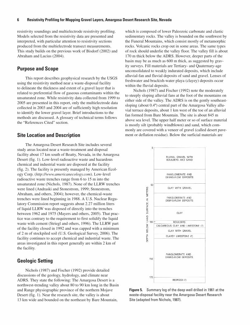
which is composed of lower Paleozoic carbonate and clastic sedimentary rocks. The valley is bounded on the southwest by the Funeral Mountains, which consist mostly of metamorphic rocks. Volcanic rocks crop out in some areas. The same types of rock should underlie the valley floor. The valley fill is about 170 m thick below the ADRS. However, deeper parts of the basin may be as much as 600 m thick, as suggested by grav-ity surveys. Fill materials are Tertiary- and Quaternary-age unconsolidated to weakly indurated deposits, which include alluvial-fan and fluvial deposits of sand and gravel. Lenses of freshwater and brackish-water playa (clayey) deposits occur within the fluvial deposits.

Nichols (1987) and Fischer (1992) note the moderately to steeply sloping alluvial fans at the foot of the mountains on either side of the valley. The ADRS is on the gently southeast-sloping (about 0.4º) central part of the Amargosa Valley allu-vial terrace deposits, about 1 km west of the toe of an alluvial fan formed from Bare Mountain. The site is about 845 m above sea level. The upper half meter or so of surface material is mostly silt (probably windblown) and sand, which com-monly are covered with a veneer of gravel (called desert pave-ment or deflation residue). Below the surficial materials are

Figure 5. Summary log of the deep well drilled in 1961 at the waste-disposal facility near the Amargosa Desert Research Site (adapted from Nichols, 1987).

http://www.americanecology.com

Method of Investigation 7

unconsolidated, moderately to poorly sorted, fluvial cobbles, gravels, sands, and silts down to depths of about 30 m. Thin, clayey lenses exist within this zone. From about 30-m depth to the valley floor are fanglomerate and debris-flow deposits with interbeds of clay, clay with sand or gravel, boulders, and clayey carbonates. There are relatively thick clayey deposits from about 50- to 60-m depth, from about 80- to 100-m depth, and from about 105- to 145-m depth (fig. 5).

Hydrologic Setting and Climate

The upper Amargosa River basin, where the ADRS is located, is part of the Amargosa hydrographic area as defined by Harrill and others (1988). The Amargosa River flows to the southeast and is the principal drainage [channel] for the Amargosa Desert. Where it approaches to within 3 km of the site, the river channel is dry more than 98 percent of the time and, on average, flows an estimated 4 to 11 hours a year (Stonestrom, Prudic, and others, 2004). In fact, no perennial streams exist within 16 km of the site. Water often flows in the Amargosa River at Beatty, about 17 km to the north (fig. 1). Surface runoff (sheet flow) occurs during intense convective downpours.

Monitoring wells within and near the disposal facility indicate the unsaturated zone ranges from 85 m thick on the east side of the facility to 110 m thick on the west side, mak-ing a step change in altitude across an apparent fault passing through the waste facility (Walvoord and others, 2005). Based on water-table level measurements in 13 wells measured dur-ing December 1988, the average hydraulic gradient is 0.06 m/m to the southwest below the LLRW disposal area and about 0.04 m/m to the south below the chemical waste dis-posal area (Fischer, 1992). Both the surface- and ground-water systems in the Amargosa River drainage basin eventually

terminate in Death Valley. Belcher and others (2002) describe the regional ground-water flow system.

Long-term average annual precipitation is a little over 11 cm per year (Johnson and others, 2007), making the Amargosa Desert one of the most arid regions in the United States. Most precipitation is transpired by the predominant plant of the sparse vegetation at the site, the creosote bush (Larrea triden-tata), or is evaporated back to the atmosphere. In the present climate, downward movement of water below about 3-m depth has not been substantiated (Johnson and others, 2007). Histori-cally, infiltration of water below about 10 m has been minimal or nonexistent for at least 6,000 to 16,000 years (Andraski and Stonestrom, 1999). The volumetric soil-water content of the top 110 m of the unsaturated zone near the southwest corner of the waste facility is shown in figure 3C. Above 40 m, the average water content was 0.09 m3/m–3; below 40 m, the aver-age water content was 0.12 m3/m–3 (Mayers and others, 2005). If enough precipitation falls to satisfy the soil-moisture deficit and the water penetrates below soil depths influenced by evap-oration and transpiration, deep percolation of water can occur and contribute to leaching and transport of contaminants.

Method of Investigation

The resistivity method (see the Glossary for definitions of selected terms used in this report) was developed early in the 1900s and is in widespread use because of its simplicity and effectiveness, the well-understood relationship between resistivity and hydrogeologic properties, and easy availability of instrumentation and interpretation tools. The method is used to determine the spatial distribution of the low-frequency resistive characteristics of the earth. Until recently, standard practice has been to drive four metal-stake electrodes into the earth. Electric current is applied to two of the electrodes, and

Figure 6. A schematic of an example electrode configuration and equipment for simple DC resistivity surveys. The distance MN is the separation between potential electrodes P1 and P2. The distance AB is the separation between current electrodes C1 and C2. Electrode separation distance (also called spacing) is typically referred to as AB/2 and MN/2, half the distances AB and MN, respectively. The control unit determines the amount of electric current applied to the C1 and C2 electrodes from a power source (battery or generator) and measures the voltage potential of the resulting electric field at the P1 and P2 electrodes. For multielectrode surveys, the control unit may also perform the automated switching between electrode pairs. To collect a resistivity sounding, the distances AB and MN are increased, about a fixed central location, to investigate deeper into the earth. For a resistivity profile, the electrode configuration and separations are held constant, to keep investigation depth relatively constant, and the entire array is moved stepwise along a path.


the electric potential is measured between the other two elec-trodes (fig. 6). Electric current is transferred from the metal stakes to the earth because of direct contact; this is called gal-vanic coupling. The stakes are arranged in a specific geometry (often symmetrically about a central location) along a (usually straight) path called a line or transect. With the help of inver-sion software, a representative resistivity structure of the earth is interpreted. Within the limits of the technique’s resolution, the method is proven and reliable in identifying areas that are relatively conductive (for example, water-saturated sediments or fine-grained or clay-rich regions) in contrast to areas that are relatively resistive (such as dry sediments or coarse-grained regions).

Resistivity of Earth Materials

Resistivity is the property of a material that opposes the flow of electric current. Resistivity is the reciprocal of electrical conductivity. The unit of resistivity is the ohm-meter (ohm-m). The resistivity of rock and sediment is dependent on several factors, including the amount of water present (water saturation), porosity, the amount of dissolved solids in the pore water (pore fluid chemistry), and mineral composition and stratification of the host rock or sediment material (lithol-ogy). All other factors being equal, dry rock is more resistive than saturated rock, and rock saturated with low-dissolved-solids water is more resistive than rock saturated with high-dissolved-solids water. High concentrations of electrically conductive minerals, such as metallic sulfides (for example, pyrite) or mineralogical clays (for example, montmorillonite), lower the bulk resistivity. Thorough discussions of the resistiv-ity method and electrical responses of earth materials can be found in Reynolds (1997), Butler (2005), Burger and others (2006), and Rubin and Hubbard (2006).

Traditional Four-Electrode Resistivity Soundings

Electrical resistivity measurements have historically been made with direct current (DC) methods that use metal stakes, called electrodes, inserted into the earth. Four electrodes, two current-transmitting (current electrodes) and two voltage-sensing (potential electrodes), are used for either vertical soundings or horizontal profiling (fig. 6). Each pair of current or potential electrodes is called a dipole. For vertical sound-ings, the electrodes are arranged symmetrically about a center, with increasing distances between pairs of electrodes used to explore greater depths. For horizontal profiles, the electrode spacing and geometry are held constant and the array of four electrodes is moved along a survey line. The applied current and the potential were measured with analog meters.

Whether using sounding or profiling techniques, an apparent resistivity is calculated for each station (the center of the array) using the geometry of the electrodes, the measured voltage and current, Ohm’s law (which associates resistivity with an electric field and current density), and the assumption

that the subsurface is an isotropic and homogeneous half-space. Apparent resistivity allows comparison of measure-ments from one area to another and provides a first approxi-mation to the actual earth resistivity. Modeling (see Glossary) is required to determine a representative electrical resistivity structure of the earth.

Automated Multielectrode Resistivity Profiling

Digital data-collection systems were developed in the 1990s that utilize dozens or even hundreds of electrodes with automated switching between electrode sets, combining aspects of both sounding and profiling. From 4 to more than 100 stainless-steel electrodes are driven a short distance into the earth along a path; usually, a constant distance separates the electrodes along a relatively straight line. Electric current is introduced into the earth by using two of these electrodes. There may be one or more channels to measure potential between pairs of other electrodes. Depending on the array type

Figure 7. Pseudosections for three electrode geometries used in automated, multielectrode resistivity surveys: A, inverse Wenner-Schlumberger array, where the current electrodes (C1 and C2) are the inner pair; B, Wenner alpha array; and C, dipole-dipole array. The triangles represent the electrodes (24 in this case) at uniform spacing in a straight line (called the “a-spacing”). The crosses (“+”) are the graphing locations (called datums), scaled by the a-spacing, for possible combinations of four electrodes for the given geometry. For each configuration, an example of a four-electrode measurement is shown, with potential electrodes P1 and P2 and current electrodes C1 and C2, and the location (circled) of where the apparent resistivity for that measurement is plotted. Note that the different geometries result in different distributions of datums. This also reflects, somewhat, the subsurface coverage. During multichannel, multielectrode surveys, there can be many pairs of potential electrodes for the pair of current electrodes in the inverse Schlumberger and dipole-dipole configurations. Advantages and limitations of the various types of arrays are discussed by M.H. Loke (available at http://www.geoelectrical.com/).

http://www.geoelectrical.com/

Data Collection 9

(see fig. 7 for three examples), an eight-channel system can measure potential simultaneously between as many as nine electrodes (one positive and eight negative for eight recorded measurements); a 10-channel system can utilize up to 11 potential electrodes.

Measurements between sets of electrodes are repeated in many combinations along the line. The arrangement of active electrodes (that is, where the current and potential electrodes are, in relation to each other) and the distance between electrodes can vary depending on the array used and the goal of the survey. Depth of investigation is increased by increas-ing the separation between the pairs of current and potential electrodes. Apparent resistivity and an earth resistivity model are determined in the standard manner (see Glossary). This method of surveying is commonly called surface imaging.

Capacitively Coupled Resistivity Profiling

A capacitor, which consists of a nonconducting material (called a dielectric) sandwiched between two conductors, is a device for storing electric charge in a circuit. Unlike a DC circuit with a capacitor, where current does not flow, alternat-ing current (AC) flows in a capacitive circuit when AC voltage is applied. Around 1999, a new resistivity system was devel-oped and marketed that does not use the metal-stake electrodes of the traditional or multielectrode resistivity systems. Instead, pairs of insulated wire cables, called dipoles, are towed along the surface in a dipole-dipole configuration (figs. 7 and 8); metallic plates can be used instead of wires. The wire cables and the earth are the “conductors” of a capacitor, and the wire insulation and air are the dielectric. An alternating cur-

rent (about 16.5 kHz for the system we used; about 12 kHz for other systems) is produced in the earth by the transmit-ter dipole, and voltage is measured by one or more receiver dipoles. The measured voltage is proportional to the resistivity of the earth between the dipoles. This electrical connection of the dipoles to the earth, that is, the transferring of an elec-tric field between the dipoles and the earth without direct or galvanic contact, is called capacitive coupling. Variations of resistivity with depth can be determined by making multiple passes over the same transect using different separations of the transmitter and receivers and different dipole lengths. Appar-ent resistivity and an earth resistivity model are determined in the standard manner. Additional details about the capacitively coupled resistivity method are available online at http://www.geometrics.com/, at http://www.iris-instruments.com/, and in Geometrics, Inc. (2001).

Data Collection

Real-Time Kinematic Global Positioning System

The Global Positioning System (GPS) is a global navigation satellite system operated and maintained by the U.S. Department of Defense. A nominal constellation of 24 satellites in high-altitude orbit transmit coded signals to GPS receivers, which measure the time taken for the signal to travel from the satellite to the receiver. The GPS system we used also measured the phase difference of carrier waves allow-ing for potentially subcentimeter positioning. Two receivers were used: one stationary, the location of which was assumed

Figure 8. A schematic of the OhmMapper capacitively coupled AC resistivity system with one transmitter dipole and two receiver dipoles arranged in an in-line, axial, dipole-dipole configuration (up to five receivers can be used simultaneously). The transmitter and each receiver contain electronics and batteries. The towed array is attached to a control console, which is usually carried by an operator or mounted on an all-terrain vehicle. Each dipole consists of two electrode cables that are plugged into opposite sides of a central electronics unit. Several lengths are available for the transmitter dipole, receiver dipoles, and the tow-link rope. Longer dipoles and increased separation between the transmitter and the receiver array promote deeper depths of investigation. Repeated passes on the same path with different dipole and tow-link rope lengths result in a set of transmitter and receiver locations that simulate the multiple electrode locations (and the different depths of investigation) of automated, multielectrode DC resistivity lines. Global Positioning System information is sent to the control unit to record the position of the array as it is towed.

http://www.iris-instruments.com/


or known, and the other a remote or “rover.” Both receivers acquired GPS data and simultaneously processed the carrier-phase tracking information in real time using a radio link to dynamically (or kinematically) establish the rover’s location. The remote receiver was positioned along the geophysical sur-vey lines to establish georeferencing, which is assigning world coordinates to the geophysical stations. Additional information about the GPS can be obtained from the U.S. Army Corps of Engineers (2003).

Resistivity Soundings

In 1999, the U.S. Geological Survey made 38 DC resis-tivity soundings at the ADRS, and an additional 16 soundings in 2000, using a standard Schlumberger array (Bisdorf, 2002). The general electrode configuration of the Schlumberger array is as shown in figure 6 with the requirement that the distance AB must be a minimum of five times greater than the distance MN. Sounding locations are shown in figure 9. For each sounding, Bisdorf (2002) presents the AB/2 spacing, the corresponding apparent resistivities, and the one-dimensional

layered-earth resistivity model. The purpose of the resistivity soundings was to confirm depth to bedrock, examine regional structure including possible faults, identify major clay layers, and locate the water table. This report examines how well these traditional resistivity soundings detect the shallow and deeper gravel layers.

Multielectrode Resistivity Profiling

In May 2003, DC resistivity measurements were made using an eight-channel resistivity imaging system, called the SuperSting R8/IP (manufactured by Advanced Geosciences Inc., Austin, Texas, USA; http://www.agiusa.com/; fig. 10), along Line A (fig. 11). See Abraham and Lucius (2004) for descriptions of the data collection. In April and May of 2004, measurements from four additional multielectrode resistiv-ity lines were collected around the waste-disposal facility to further define the extent and depth of the lower gravel layer detected in Line A; these are Lines B – E in figure 11. Table 1 summarizes the data-collection parameters.

Figure 9. Location map of the Schlumberger soundings (black circles) and the multielectrode resistivity lines (A through E; red lines). The soundings from 1999 are numbered 1 through 38; the soundings from 2000 are numbered 101 through 116. Adapted from Bisdorf (2002).

http://www.agiusa.com/

Data Collection 11

Figure 10. A, Control unit for the AGI SuperSting R8/IP multielectrode resistivity system sitting in the back seat of a field vehicle. Power source is one or two 12-volt batteries. The yellow cables connect the control unit to the electrodes. B, Stainless-steel stake, driven about 0.3 meter into the earth, with a computer-addressable electrode fastened to it for use with the SuperSting R8/IP.

Figure 11. Location map of the resistivity lines (blue lines) near the waste storage facility. Multielectrode DC resistivity data were collected along Lines A–E. Line A is the same as the “SEIS” line at the upland interfluvial site in Abraham and Lucius (2004). Capacitively coupled AC resistivity data were collected on the south, west, north, and east access roads next to the waste-disposal facility


Capacitively Coupled Resistivity Profiling

Capacitively coupled AC resistivity data were collected in April 2005 using the OhmMapper TR5 system (manufac-tured by Geometrics, Inc., San Jose, California, USA; http://www.geometrics.com/) towed by an all-terrain vehicle (figs. 12 and 13). Data were collected just outside the perim-eter of the storage facility on the access roads — the South,

West, North, and East Rd Lines in figure 11. All data were col-

lected using five receiver dipoles. Repeated passes with

different dipole and tow-link rope lengths on these lines simu-

late the multiple electrode locations (and the different depths

of investigation) of automated multielectrode DC resistivity

profiling. Other important data-collection parameters are

summarized in table 2.

Figure 12. The OhmMapper system is configured here to be towed by an all-terrain vehicle (ATV). This picture shows how the complete data-acquisition system is attached to the ATV. The radio antenna permits the mobile GPS receiver (shown here) to maintain communication with the base station GPS receiver (not shown) in order to determine real-time global positioning of the mobile receiver.

Figure 13. The OhmMapper system is shown here with five receiver dipoles and the transmitter dipole being towed by an all-terrain vehicle.

http://www.geometrics.com/

Data Processing and Modeling 13

Data Processing and Modeling

Processing consists of manipulating the data to facilitate interpretation. This can involve the following:

Improving the signal-to-noise ratio (for example, by •using the average of repeat measurements)

Editing (removing) data according to some criteria, •such as minimum voltage or voltage/current levels, an obvious nonfunctioning electrode, or noise (usually due to high contact resistance between the electrode and earth)

Applying corrections for known perturbations of •apparent resistivity (often associated with changing the MN/2 distance in traditional Schlumberger soundings)

Rearranging, binning, or interpolating measurements or •apparent resistivities

Attaching elevation and traverse distance for use in •modeling and display

Georeferencing can occur during data collection or at some point in the data-processing sequence. Since the GPS provides location in latitude and longitude, GPS data are projected onto a rectangular grid for some processing opera-tions and for visualization. The Universal Transverse Mercator

(UTM) projection, in meters, is used for all surveys described in this report: NAD27 UTM zone 11N. All elevations are given in meters above sea level and referenced to the National Geodetic Vertical Datum 1929 (NGVD29).

Modeling starts with converting the measurements asso-ciated with a particular set of four electrodes to an apparent resistivity (r

a). An inversion algorithm uses these apparent

resistivities and the electrode (or dipole) configuration to produce an initial model of resistivity in the earth that is a one-dimensional (1-D) sequence for traditional sounding or a two-dimensional (2-D) distribution for multielectrode profil-ing. Using the model, apparent resistivity is calculated (called model r

a) and compared to the apparent resistivity calculated

directly from the field measurements (called observed ra). The

inversion process modifies the model and then recalculates model r

a for comparison to the observed r

a. This iterative

process is repeated until the difference between the model and observed apparent resistivities is less than some acceptable error value (usually in percent). Between iterations, one or more model nodes may be deleted if a realistic match of model r

a and observed r

a cannot be made.

Bisdorf (2002) explains the data processing and inter-pretation of the resistivity soundings. In brief, the automated interpretation program of Zohdy and Bisdorf (1989) was used to produce 1-D resistivity models that fit the field-data appar-ent resistivities within some acceptable error range. Selected models are shown in figure 14.

Figure 14. Selected one-dimensional resistivity models derived from the soundings in Bisdorf (2002). View is to the southwest. Thick black lines indicate the rectangular boundary of the waste-disposal facility. OHM-M, ohm-meters.


LineElectrodespacing(meters)

Totallength

(meters)

Current(milliamp)

Cycletime

(seconds)

A 5 1,150 400 – 750 7.2

B 4 1,240 500 – 1,000 0.8

C 4 1,036 500 – 1,000 0.8

D 4 900 500 – 1,000 0.8

E 4 600 500 – 1,000 0.8

Table 1. Selected parameters for the multielectrode DC resistivity data collection along Lines A–E (figs. 11 and 15). For all lines, electrodes were wetted with a sodium chloride solution to improve electrical contact with the extremely dry surface sediments. Eighty-electrode spreads were used on Line A; Lines B–E used 76-electrode spreads. The separation distance between electrodes (called the electrode spacing) was held constant for each line. The inverse Schlumberger array type was used for all five lines (see fig. 7). Two current electrodes and two to eight potential electrodes were used — half of each on either side of a central point. Lines consisted of overlapping spreads. After a suite of measurements was collected from a spread of electrodes, a section of electrodes was moved from the beginning of the spread to the end, extending the data coverage along the line beyond what was just collected. This data-collection technique allows for the collection of a profile of soundings along long lines without sacrificing resolution or depth of investigation. Three alternating positive and negative current pulses were used: a positive pulse of time T, a negative pulse of time 2T, and another positive pulse of time T. The cycle time is the total time for all three pulses (4T in this case).

Table 2. Selected parameters for the capacitively coupled AC resistivity data collection at the border of the waste-disposal facility (figs. 11 and 16). For all lines, electrodes were configured as in-line, axial, dipole-dipole arrays (see figs. 7 and 8) with multiple dipole- and rope-length geometries. Because of the continuous tow and the need for uniform measurement spacing in the two-dimensional inversion software, the integrated GPS location information was used to average the field measurements into bins that are 2.5 meters wide.

LineDipolelength

(meters)

Tow-linkrope length

(meters)

Linelength

(meters)

North Rd 510

2.5, 5 10, 30

882

East Rd 510

2.5, 5 10, 30

386

South Rd 510

2.5, 5 10, 30

851

West Rd 510

2.5, 5 10, 30

455

Conclusions 15

For the multielectrode and capacitively coupled resistiv-ity profiling, the field measurements, either before or after some processing has been performed, are used as input into the computer program EarthImager 2D manufactured by Advanced Geosciences, Inc. The EarthImager 2D calculates the apparent resistivities and performs the inversion to produce 2-D models called resistivity sections. Elevation from the geo-referenced measurement locations can be incorporated into the inversion. The EarthImager 2D instruction manual (Advanced Geosciences, Inc., 2007) and notes and papers by M.H. Loke (available at http://www.geoelectrical.com/) discuss the inver-sion process in detail. The Appendix shows the results of the EarthImager 2D inversions for Lines A–E as observed and model apparent resistivity (in pseudosection format) and the resistivity section.

Resistivity sections for the five multielectrode resistiv-ity lines on Lines A–E near the waste-disposal facility are shown in figure 15. Depth of investigation is as great as 65 m. Reddish colors indicate high resistivity in the models and are associated with the gravel in the near-surface sediments and with the lower gravel layer.

Resistivity sections for the four capacitively coupled resistivity lines positioned adjacent to the waste-disposal facility boundary (the South, West, North, and East Rd Lines) are shown in figure 16. Depth of investigation is about 10 m; therefore, the lower gravel layer is not detected. High resistiv-ity is associated with the near-surface sediments.

Conclusions

This report shows that multielectrode resistivity profiling can image hydrogeologic features in the arid environment near the ADRS to a depth of about 65 m in some locations. Four discontinuous layers with variable thicknesses are identified in the resistivity cross sections (figs. 15 and 16) and in figure 17, which shows a generalized stratigraphic model derived from the average resistivity for the upper 65 m of alluvium along Lines A–E. Also in figure 17 are water-content charts that show a moderate inverse correlation with the average resistiv-ity. The lack of a strong inverse correlation is likely due to the localized nature of lenses and layers where the water-content data were collected and the generalized nature of the resistivity plot. Despite the lack of strong inverse correlation with water content, higher resistivity strongly correlates with gaseous contaminant concentration at about 20-m depth (compare with fig. 4).

The four generalized layers interpreted from the average resistivity plot in figure 17 can be described as follows:

At the surface there are very dry deposits that have resistivities from about 85 to over 400 ohm-m. Trenching and drilling show these sediments grade for about 2.2 m from fine-grained deposits into coarser and gravel-sized rocks (see, for example, fig. 11 in Fischer, 1992).

A relatively conductive layer, in the range of about 44 to 70 ohm-m, lies beneath the near-surface materials and is 5 to 15 m thick. Fischer (1992) describes these sediments as poorly to moderately sorted sand, gravel, and cobble.

A relatively resistive layer, of variable thickness, lies within a depth range of about 15 to 30 m. Resistivity is between about 85 and 120 ohm-m. Sediments of this layer are generally less moist than sediments above and below (fig. 3C). Based on observations of Striegl and others (1996), the higher resistivities, and the reduced water content, gravel likely is present in this layer. In addition, as shown in figure 4, this zone has the highest concentrations of gaseous contaminants.

Relatively conductive sediments are below the gravel layer with resistivity ranging from about 40 to 60 ohm-m. These sediments likely are finer grained deposits. They have decreasing resistivity with depth that probably correlates with increasing moisture content with depth (compare to fig. 3C).

A three-dimensional (3-D) view of the resistivity sections is shown in figure 18. Lines A–E are sections inverted from the multielectrode resistivity (SuperSting) measurements. The South, West, North, and East Rd Lines are sections inverted from the capacitively coupled resistivity (OhmMapper) measurements. Resistivity of about 85 ohm-m or greater is indicated by reddish colors. These areas of higher resistivity most likely correspond with the dry surface material and with the lower gravel layer.

The lower gravel layer thins and disappears toward the southeast (near the intersection of Line A and Line D). An isolated, uplifted area supported by bedrock is a few hundred meters to the southeast of the facility. The thinning and then disappearance of the gravel layer suggests that the alluvium may have built up gradually around the bedrock, with more recent alluvial deposition covering more and more of the uplift.

Figure 19 is another 3-D view of the resistivity sections along with selected 1-D models produced from the four-elec-trode soundings of Bisdorf (2002). On the resistivity sections, only values greater than 85 ohm-m are shown (red and black). The black areas are our interpretation of the extent and thick-ness of the lower gravel layer. The break in the layer at the northeast corner of the site (the intersection of the East Rd and North Rd Lines) is related to the break in data collection over the facility entrance road. We believe that the gravel layer that is indicated in Line D and Line E continues under the entrance road (dashed lines in fig. 19). The 1-D models are in general agreement with the resistivity sections, with many models having a thin high-resistivity layer at the surface and a thicker high-resistivity layer at shallow depth. The thinning and disap-pearance of the lower gravel layer near the southeast corner of the site also are suggested in the 1-D models.

At the ADRS, the application of multielectrode resistivity imaging successfully delineated the depth and lateral extent of gravel layers associated with gaseous contaminant transport. Toward the southeast corner of the study area, the lower gravel layer thins and then disappears against what may have been higher deposits or exposed bedrock during gravel deposition.


Figure 15. Resistivity sections along the five multielectrode resistivity lines (SuperSting R8/IP) near the waste-disposal facility at the Amargosa Desert Research Site. Distance on the horizontal axis is from the start of the line. Location of lines is shown in figure 11. OHM-M, ohm-meters.

Conclusions 17

Figure 16. Resistivity sections along the four capacitively coupled resistivity lines (OhmMapper) at the waste-disposal facility boundary at the Amargosa Desert Research Site. Location of lines is shown in figure 11. OHM-M, ohm-meters.


This study illustrates that multielectrode resistivity surveying is a practical, noninvasive method to image the hydrogeologic features to a depth of about 65 m in the arid environment of the Amargosa Desert. Capacitively coupled resistivity surveys are useful for mapping lithologic variations in the upper 6 to 10 m. Traditional four-electrode resistivity soundings can be useful for determining regional structures, but they would be too time consuming and expensive for effectively map-ping relatively shallow gravel layers across the entire site.

Resistivity variations have a moderate inverse correlation with

subsurface moisture variations. However, gaseous contaminant

concentration strongly correlates with the mapped gravel layer

between 15- and 30-m depths. The interpreted location of the

gravel layers, along with additional surveys, could be used to

create sitewide geoelectric and stratigraphic models, as well

as mapping the sitewide distribution of possible pathways for

gaseous contaminant transport in the subsurface.

Figure 17. An average-resistivity model and a generalized stratigraphic model derived from the average resistivity for the Amargosa Desert Research Site area. To calculate the average resistivity for the upper 65 meters of the surveyed alluvium, the values in the resistivity models for Lines A–E were combined along rows of the same depth. The water-content charts, generalized stratigraphic model, and resistivity plot have the same vertical scale. The matching of surface elevations is approximate. The water-content chart on the right is adapted from Johnson and others (2007) for data collected annually from 2001 to 2005 in neutron-probe access tube VS2 approximately 45 meters north of UZB-2. The inset water-content chart is adapted from Mayers and others (2005) for data collected in 1999 in UZB-3. See figure 11 for locations of UZB-2 and ZB-3. M3/M3, cubic meter per cubic meter.

Conclusions 19

Figure 18. A three-dimensional view of resistivity sections near the Amargosa Desert Research Site. Lines A–E note the location of automated multielectrode DC resistivity profiles. The capacitively coupled AC resistivity profiles were along the South, West, North, and East Rd Lines at the boundary of the waste-disposal facility. Reddish colors indicate areas of higher resistivity that are relatively dry deposits. OHM-M, ohm-meters.


Figure 19. A three-dimensional view of resistivity sections and selected one-dimensional resistivity models near the Amargosa Desert Research Site. On the resistivity sections, only values greater thann 85 ohm-m are shown (red and black), indicating drier deposits. The interpreted lower gravel layer is shown by the black areas. Dashed lines indicate inferred extent of the gravel layer. OHM-M, ohm-meters.

References Cited 21

Acknowledgments

The authors thank Brian J. Andraski, David A. Stone-strom, and David E. Prudic of the USGS Amargosa Desert Research Site Team for their interpretations of the resistivity data in terms of geologic context and implications, and for their thoughtful comments during the preparation and revision of this document.

References Cited

Abraham, J.D., and Lucius, J.E., 2004, Direct current resistiv-ity profiling to study distribution of water in the unsaturated zone near the Amargosa Desert Research Site, Nevada: U.S. Geological Survey Open-File Report 2004–1319, 16 p. [accessed September 18, 2007 http://pubs.usgs.gov/of/2004/1319/ ]

AGI (Advanced Geosciences, Inc.), 2007, Instruction manual for EarthImager 2D, version 2.2.0—Resistivity and IP inversion software: Advanced Geosciences, Inc., Austin, Texas, 134 p. [accessed September 18, 2008 http://www.agiusa.com/]

Andraski, B.J., and Stonestrom, D.A., 1999, Overview of research on water, gas, and radionuclide transport at the Amargosa Desert Research Site, Nevada, in Morganwalp, D.W., and Buxton, H.T., eds., U.S. Geological Survey Toxic Substances Hydrology Program, Proceedings of the Techni-cal Meeting, Charleston, South Carolina, March 8–12, 1999, v. 3, Subsurface Contamination from Point Sources: U.S. Geological Survey Water-Resources Investigations Report 99–4018C, p. 459–465.

Andraski, B.J., Stonestrom, D.A., Michel, R.L., Halford, K.J., and Radyk, J.C., 2005, Plant-based plume-scale mapping of tritium contamination in desert soils: Vadose Zone Journal, v. 4, p. 819–827.

Belcher, W.R., Faunt, C.C., and D’Agnese, F.A., 2002, Three-dimensional hydrogeologic framework model for use with a steady-state numerical ground-water flow model of the Death Valley regional flow system, Nevada and California: U.S. Geological Survey Water-Resources Investigations Report 2001–4254, 87 p.

Bisdorf, R.J., 2002, Schlumberger soundings at the Amargosa Desert Research Site, Nevada: U.S. Geological Survey Open-File Report 2002–140, 65 p. [accessed September 18, 2007 http://pubs.usgs.gov/of/2002/ofr-02-0140/ ].

Burger, H.R., Sheehan, A.F., and Jones, C.H., 2006, Introduc-tion to applied geophysics—Exploring the shallow subsur-face: New York, Norton, 554 p.

Butler, D.K., ed., 2005, Near-surface geophysics: Tulsa, Okla., USA, Society of Exploration Geophysicists, 732 p.

Dolezalek, H., Tammet, H., Latham, J., and Uman, M.A., 2004, Atmospheric electricity, in Lide, D.R., editor-in-chief, CRC Handbook of Chemistry and Physics (85th ed., 2004-2005): New York, CRC Press, p. 14–23—14–40.

Fischer, J.M., 1992, Sediment properties and water movement through shallow unsaturated alluvium at an arid site for disposal of low-level radioactive wastes near Beatty, Nye County, Nevada: U.S. Geological Survey Water-Resources Investigations Report 92–4032, 48 p.

Geometrics, Inc., 2001, OhmMapper TR5 29005–01 Rev. F, Operation Manual: San Jose, Calif., Geometrics, Inc., 147 p. [accessed September 18, 2007 http://www.geometrics.com/]

Harrill, J.R., Gates, J.S., and Thomas, J.M., 1988, Major ground-water flow systems in the Great Basin region of Nevada, Utah, and adjacent states: U.S. Geological Sur-vey Hydrologic Investigations Atlas HA–694–C, scale 1:1,000,000.

Healy, R.W., Striegl, R.G., Michel, R.L., Prudic, D.E., and Andraski, B.J., 1999, Tritium in water vapor in the shallow unsaturated zone at the Amargosa Desert Research Site, in Morganwalp, D.W., and Buxton, H.T., eds., U.S. Geological Survey Toxic Substances Hydrology Program, Proceed-ings of the Technical Meeting, Charleston, South Carolina, March 8–12, 1999, v. 3, Subsurface Contamination from Point Sources: U.S. Geological Survey Water-Resources Investigations Report 99–4018C, p. 485–490.

Johnson, M.J., Mayers, C.J., Garcia, C.A., and Andraski, B.J., 2007, Selected micrometeorological, soil-moisture, and evapotranspiration data at Amargosa Desert Research Site in Nye County near Beatty, Nevada, 2001–05: U.S. Geo-logical Survey Data Series 284, 28 p.

Mayers, C.J., Andraski, B.J., Cooper, C.A., Wheatcraft, S.W., Stonestrom, D.A., and Michel, R.L., 2005, Modeling tritium transport through a deep unsaturated zone in an arid envi-ronment: Vadose Zone Journal, v. 4, p. 967–976.

Nichols, W.D., 1987, Geohydrology of the unsaturated zone at the burial site for low-level radioactive waste near Beatty, Nye County, Nevada: U.S. Geological Survey Water-Supply Paper 2312, 57 p.

Prudic, D.E., Stonestrom, D.A., and Striegl, R.G., 1997, Tri-tium, deuterium, and oxygen-18 in water collected from the unsaturated sediments near the low-level radioactive-waste burial site south of Beatty, Nevada: U.S. Geological Survey Water-Resources Investigations Report 97–4062, 23 p.

Reynolds, J.M., 1997, An introduction to applied and environ-mental geophysics: Chichester, England, Wiley, 796 p.

http://pubs.usgs.gov/of/2004/1319/

http://pubs.usgs.gov/of/2004/1319/



http://pubs.usgs.gov/of/2002/ofr-02-0140/

http://www.geometrics.com/


Rubin, Y., and Hubbard, S.S., eds., 2006, Hydrogeophysics, Water Science and Technology Library, v. 50: Dordrecht, The Netherlands, Springer, 523 p.

Sheriff, R.E., 2002, Encyclopedic dictionary of applied geophysics (4th ed.): Tulsa, Okla., Society of Exploration Geophysicists, 429 p.

Stonestrom, D.A., Abraham, J.D., Andraski, B.J., Baker, R.J., Mayers, C.J., Michel, R.L., Prudic, D.E., Striegl, R.G., and Walvoord, M.A., 2004, Monitoring radionuclide contamination in the unsaturated zone—Lessons learned at the Amargosa Desert Research Site, Nye County, Nevada: Proceedings, Workshop on long-term performance monitor-ing of metals and radionuclides in the subsurface, Reston, Va., April 20–22, 2004.

Stonestrom, D.A., Abraham, J.D., Lucius, J.E., and Prudic, D.E., 2003, Focused subsurface flow in the Amargosa Des-ert characterized by direct-current resistivity profiling: Eos Transactions, American Geophysical Union, v. 84, no. 46, Fall Meeting Supplement, Abstract H31B–0467.

Stonestrom, D.A., Prudic, D.E., Laczniak, R.J., and Akstin, K.C., 2004, Tectonic, climatic, and land-use controls on ground-water recharge in an arid alluvial basin—Amargosa Desert, U.S.A., in Hogan, J.F., Phillips, F.M., and Scanlon, B.R., eds., Groundwater recharge in a desert environment—The Southwestern United States: American Geophysical Union, Water Science and Applications Series, v. 9, p. 29–47.

Stonestrom, D.A., Prudic, D.E., Laczniak, R.J., Akstin, K.C., Boyd, R.A., and Henkelman, K.K., 2003, Estimates of deep percolation beneath native vegetation, irrigated fields, and the Amargosa River channel, Amargosa Desert, Nye County, Nevada: U.S. Geological Survey Open-File Report 2003–104, 83 p. [accessed September 18, 2007 http://pubs.usgs.gov/of/2003/ofr03-104/ ]

Striegl, R.G., Prudic, D.E., Duval, J.S., Healy, R.W., Landa, E.R., Pollock, D.W., Thorstenson, D.C., and Weeks, E.P., 1996, Factors affecting tritium and 14carbon distributions in the unsaturated zone near the low-level radioactive-waste burial site south of Beatty, Nevada: U.S. Geological Survey Open-File Report 96–110, 16 p.

U.S. Army Corps of Engineers, 2003, NAVSTAR global positioning system surveying: Department of the Army, U.S. Army Corp of Engineers, Engineer Manual EM 1110–1–1003, various pagination. [accessed September 18, 2007 http://www.usace.army.mil/publications/eng-manuals/

U.S. Geological Survey, 2006, Toxic Substances Hydrology Program—Amargosa Desert Research Site—Site Descrip-tion. [accessed September 18, 2007 http://nevada.usgs.gov/adrs/site.htm].

Walvoord, M.A., Striegl, R.G., Prudic, D.E., and Stonestrom, D.A., 2005, CO

2 dynamics in the Amargosa Desert—

Fluxes and isotopic speciation in a deep unsaturated zone: Water Resources Research, v. 41, W02006, 15 p.

Zohdy, A.A.R., and Bisdorf, R.J., 1989, Programs for the automatic processing and interpretation of Schlumberger sounding curves in QuickBASIC 4.0: U.S. Geological Survey Open-File Report 89–137, A&B, 64 p. + diskette.

http://pubs.usgs.gov/of/2003/ofr03-104/

http://pubs.usgs.gov/of/2003/ofr03-104/

http://www.usace.army.mil/publications/eng-manuals

http://nevada.usgs.gov/adrs/site.htm

http://nevada.usgs.gov/adrs/site.htm

Glossary 23

Glossary

Definitions have been adapted from Reynolds (1997), Sheriff (2002), http://en.wikipedia.org/, and other sources.

Alternating current Alternating current is an electric current where magnitude and direction of the current changes (reverses) cyclically over time. Alternating current always produces an alternating magnetic field. There will be an associated alternating electric field in nearby conductors. Alternating current is commonly used in houses and offices.

Apparent resistivity Apparent resistivity is the electrical resistivity of isotropic, homogeneous earth that would produce the same response (voltage and current relationships) as was measured in the field using a single four-electrode array.

Apparent resistivity = KIV

,

where V is the measured potential in volts, I is the applied current in amperes, and K is the geometric factor. Apparent resistivity allows comparison of measurements from one area to another and provides a first approximation to the actual earth resistivity. Modeling is required to determine a representative electrical resistivity structure of the earth.

Conduction current Conduction current is an electric current produced by an applied voltage difference or an electric field.

Direct current Direct current is an electric current where the flow of electric charge (such as electrons or ions) through a conductor is in one direction from high to low electric potential. Direct current always produces a magnetic field. Direct current is sometimes called galvanic current. Direct current is commonly used to run certain types of equipment and is produced by batteries.

Electric current Electric current is the movement of electrically charged particles, such as electrons or ions, through conductors. Electric current produces a magnetic field. Because electrical charge is involved, an electric field also exists. The unit for current is the ampere.

Electric field An electric field is produced by the presence of electrical charge, such as an electron or ion. An electric field contains electrical energy. An electric field can be static (strength does not change over time) or varying (strength changes over time). Common units for an electric field are volt per meter or Newton per coulomb.

Electric potential Electric potential is the stored energy (or potential energy) per unit electric charge associated with a static (or constant) electric field. It is measured in volts. Electric potential (or voltage) is only physically meaningful when measured between two different locations.

Electrical conductivity Electrical conductivity is the ability of a material to conduct electric current and is the reciprocal of electrical resistivity. Units are siemens per meter (S/m); a siemens is an ampere per volt, the reciprocal of ohm. Electrical conductivity affects the attenuation of electromagnetic fields. Where electrical conductivity is near zero, such as in air, which is about 3x10–14 S/m (Dolezalek and others, 2004), electromagnetic (EM) waves can travel great distances, but electric current generally cannot flow. In the earth, where electrical conductivity is often greater than 0.01 to 0.1 S/m, EM waves propagate relatively short distances, but electric current flows readily.

Electrical methods Electrical methods measure electric potential (voltage) produced by electric current in the earth. Current in earth materials is controlled by the fundamental material property called electrical conductivity. Because most dry rocks and sediments are poor conductors of electricity, their conductivity is generally determined by the quality and quantity of water in the pore space, the connectedness of the pores, and the relative abundance of clay minerals. Electrical conduction in conductive rocks and sediments principally occurs in two ways: electrolytic (or ionic), such as the movement of ions in water, and electronic (or ohmic), such as the movement of charge carriers (for example, free electrons) in metals or clays. A third form of limited conduction, called displacement or dielectric conduction, occurs in media with low conductivity.

As electric current passes through conductive earth, it always produces both a magnetic field and an electric field. These fields can cause electrical polarization. The four common forms of electrical polarization include electronic (net displacement of the electron cloud with respect to the nucleus of an atom), ionic (displacement of charged atoms or molecules with respect to each other), orientational (aligning of molecules with asymmetrical charge distributions, such as water molecules), and interfacial (local accumulations of migrating charge against a chemical or electrical barrier). The electrical methods focus on the electric field and sometimes on polarizations produced by charge flow.

Electrical methods include resistivity, self potential (also called spontaneous potential), induced polarization, and seismoelectric.

Electromagnetic field An electromagnetic (EM) field is composed of two related fields: the electric field and the magnetic field. Typically, the strength of the two fields changes over time, alternating in strength in a cyclic and synchronized manner. A changing electric field produces a changing magnetic field; likewise, a changing magnetic field produces a changing electric field. The number of cycles per second is called the frequency (usually measured in hertz [Hz], which is one cycle per second). Electromagnetic properties affect the propagation (or transmission) and attenuation of

http://en.wikipedia.org/


EM fields. An EM field cannot propagate for any great distance in conductive media such as typical rocks and sediments because the electric field causes electric current (also called conduction current) and rapid dissipation of the energy into heat. When an EM field occurs in media with low conductivity, such as air, ice, or resistive sediments, it travels or propagates as an electromagnetic wave; a radio wave is a common example.

Electromagnetic properties Electromagnetic properties affect the propagation and attenuation of electromagnetic fields. The three properties are electrical conductivity, dielectric permittivity, and magnetic permeability. The speed of EM waves is determined mostly by dielectric permittivity. In most earth materials, the attenuation (or reduction in strength) of EM waves is determined primarily by electrical conductivity.

Energy Energy is the capacity to do work. All physical systems possess this fundamental quantity. Energy is defined as the amount of work required to change the state of a system from one position or level to another position or level.

Equivalence Equivalence means that a layer can produce nearly the same geophysical response for a variety of combinations of thickness and property magnitude. This is particularly true with the electrical, electromagnetic, and potential-field methods. For example, nearly the same electric current flows in two different resistive layers if the product of their thickness and resistivity are similar. Equivalence issues may be overcome using additional geologic or geophysical information. Equivalence is less of a problem with wave-based methods such as ground-penetrating radar and seismic methods.

Geometric factor The geometric factor is the collection of geometric terms derived from the relative position of four electrodes (two current and two potential). It is used to determine the voltage difference between two potential electrodes in the electric field produced by two current electrodes on a flat and uniform (homogeneous and isotropic) earth:

where V is the voltage difference, I is the applied current, ra

is the apparent resistivity (the resistivity of a flat, uniform earth), AM and BM are the distances from potential point M to current points A and B, and AN and BN are the distances from potential point N to current points A and B. Rearranging the expression above produces the equation used to determine apparent resistivity and the geometric factor, K:

Inversion Inversion is the process of determining a

model, or distribution, of earth properties from geophysical measurements or observations. The model or distribution may not be unique. The model itself may be called an inversion.

Magnetic field A magnetic field is the effect produced by moving electric charges. It is also called magnetic intensity, magnetic induction, or magnetic flux density. A magnetic field contains magnetic energy. Unlike electric fields, magnetic fields have no related “magnetic charges.” A magnetic field that changes in strength over time produces an electric current in nearby conductors. The unit of magnetic field strength is either the tesla or gauss.

Model, modeling With respect to geophysical interpretation, a model is a conceptual or mathematical representation of the distribution of earth physical properties from which effects can be calculated for comparison to geophysical measurements and observations. However, agreement between the actual field data and the computed data from a model does not prove or validate the model. Models usually lack uniqueness and typically are simplifications of the actual distribution of properties in the earth. A model is used to provide a better understanding of the field observations. Forward modeling (the solution of a direct problem) calculates or predicts field measurements or observations for a given distribution of properties. Inverse modeling (the solution of an inverse problem) determines the distribution of properties (the model) that matches field measurements or observations within a given tolerance.

Pseudosection A pseudosection is a standard plotting convention of an electrical measurement or calculation, usually apparent resistivity, as a function of electrode geometry. It is related to depth of investigation but does not represent a distribution of electrical properties in the earth. See figure 7 for examples of pseudosection nodal assignments called datums, and figures A1–A5 for example pseudosections. A datum is located at the “median depth of investigation,” where the section of the earth above this depth has the same influence on measured potential as the section below this depth.

Resistivity Electrical resistivity is that property of a material that resists the flow of electric current. Resistance converts electrical energy into heat, leading to a loss of electric potential or electric current. Electrical resistivity is the ratio of the electric field intensity to the electric current density. Resistivity is commonly expressed in ohm-meters, where an ohm is one volt per ampere of current. The resistivity of earth material covers a broad range. In general, soil, clay, and shale have low resistivity; sand and gravel have high resistivity, and limestone and some igneous rocks can have even higher resistivity. However, the amount and type of water in the material can drastically affect a material’s bulk resistivity. A resistive rock at one location may appear as a conductor at another location if it is saturated with saline water.

, where .

,

+--=

BNANBMAMI

V a 11112

KI

Va = K = 2

1

AM-

1

BM-

1

AN+

1

BN

-1

Appendix 25

Resistivity profiling, profile Resistivity profiling is a measurement collection technique with the objective of determining how measurements, and eventually resistivity after modeling, vary vertically and laterally with location. Originally, profiling referred to a method where the electrode arrangement and separation were constant, and so depth of investigation was relatively constant, and the entire array was moved progressively along a line or transect. With the use of automated switching and multielectrode arrays, profiling now combines both soundings and traditional profiling so that vertical and horizontal variations of resistivity can be determined. The resulting two-dimensional resistivity model commonly is called a resistivity section or profile and represents a vertical slice through the earth.

Resistivity sounding A resistivity sounding collects a series of electrical resistivity measurements using successively increasing electrode separation distance about a central location. A software program determines a layered-earth resistivity structure at that single location from the apparent resistivity associated with the various electrode separations. This model is often referred to as one-dimensional because it provides resistivity information directly below the central

location, similar to core sample information from a borehole or well.

Appendix

Inversion results from the EarthImager 2D software (Advanced Geosciences, Inc., 2007) are presented for the multielectrode DC resistivity profiles. In each figure, the top image is a pseudosection of observed apparent resistivity (calculated from the field measurements), the middle image is a pseudosection of model apparent resistivity (calculated from the inverted resistivity section), and the lower image is the inverted resistivity section. Color scales for resistity and apparent resistivity can differ from image to image and from figure to figure because the software automatically assigns the limits of the color scale. The horizontal scale is the distance in meters from the start of the line. The small black dots in the pseudosections are the datums used in the inversion. Some datums are missing because the electrode geometry required for that datum location was not part of the automated acquisi-tion; other datums are missing because a realistic match of observed and model apparent resistivity could not be made.


Figure A1. Line A inversion results. OHM-M, ohm-meters; APPROX., approximate.

Appendix 27

Figure A2. Line B inversion results. OHM-M, ohm-meters; APPROX., approximate.


Figure A3. Line C inversion results. OHM-M, ohm-meters; APPROX., approximate.

Appendix 29

Figure A4. Line D inversion results. OHM-M, ohm-meters; APPROX., approximate.


Figure A5. Line E inversion results. OHM-M, ohm-meters; APPROX., approximate.

Lucius and others—Resistivity Profiling for M

apping Gravel Layers, A

margosa D

esert Research Site, Nevada—

Scientific Investigations Report 2008-5091

resistivity profiling for mapping gravel layers that … of earth materials ... resistivity...

Documents