resolution enhancement of ultrasonic …...figure 2.5 automated ultrasonic testing setup for pipe...
TRANSCRIPT

RESOLUTION ENHANCEMENT OF ULTRASONIC SIGNALS USING AUTOREGRESSIVE SPECTRAL
EXTRAPOLATION
by
Babak Shakibi
A thesis submitted in conformity with the requirements for the degree of Master of Applied Science
Department of Mechanical and Industrial Engineering University of Toronto
© Copyright by Babak Shakibi 2011

ii
RESOLUTION ENHANCEMENT OF ULTRASONIC SIGNALS
USING AUTOREGRESSIVE SPECTRAL EXTRAPOLATION
Babak Shakibi
Master of Applied Science
Mechanical and Industrial Engineering University of Toronto
2011
Abstract
Time of Flight Diffraction (TOFD) is one of the most accurate ultrasonic methods for crack
detection and sizing in pipeline girth welds. Its performance, however, is limited by the temporal
resolution of the signal. In this thesis, we develop a signal processing method based on
autoregressive spectral extrapolation to improve the temporal resolution of ultrasonic signals.
The original method cannot be used in industrial applications since its performance is highly
dependent on selection of a number of free parameters. This method is modified by optimizing
its various steps and limiting the number of free parameters, and an automated algorithm for
selection of values for the remaining free parameters is proposed based on the analysis of a large
set of synthetic signals. The performance of the final algorithm is evaluated using experimental
data; it is shown that the uncertainty in crack sizing accuracy can be reduced by as much as 80%.
Furthermore, the proposed method is shown to be capable of resolving overlapping echoes;
therefore, smaller cracks that have echoes that are not clearly resolved in the raw signal, can be
detected and sized in the enhanced signal.

iii
Acknowledgments
First of all I would like to express my sincere gratitude to my supervisor, Prof. Anthony Sinclair,
for his guidance and support without which this thesis would not have been possible. I would
also like to thank my industrial supervisor, Dr. Michael Moles, who supported my research in
numerous ways.
I am grateful to the National Science and Engineering Research Council of Canada (NSERC),
Mathematics of Information Technology and Complex Systems (MITACS), and Olympus NDT
Canada for sponsoring my research and more importantly, for giving me a distinguished
opportunity to work on a rewarding academic/industrial collaborative research project.
I would also like to express my gratitude to Robert Ginzel, Edward Ginzel and the team at
Eclipse Scientific particularly, David Cziraki, Larry Etherington and Steve McCarley for their
help in the experimental part of my research. Working with them was an invaluable experience
for me.
Finally, I particularly thank my family for their support and encouragement throughout the
course of my thesis.

iv
Table of Contents
Abstract .......................................................................................................................................... iii
Acknowledgments .......................................................................................................................... iii
Table of Contents ........................................................................................................................... iv
List of Figures ................................................................................................................................ vi
List of Symbols .............................................................................................................................. xi
1 Introduction .............................................................................................................................. 1
2 Background Theory and Literature Review.......................................................................... 4
2.1 Propagation of Mechanical Waves in Elastic Media .......................................................... 4
2.2 Reflection and Refraction ................................................................................................... 5
2.3 Use of Ultrasound in Nondestructive Testing ..................................................................... 7
2.3.1 Display Methods ..................................................................................................... 8
2.4 Ultrasonic NDT for Pipeline Girth Weld Testing ............................................................. 10
2.4.1 Manual Ultrasonic Testing .................................................................................... 10
2.4.2 Automated Ultrasonic Testing .............................................................................. 10
2.4.3 Ultrasonic Testing Using Phased Arrays .............................................................. 11
2.5 Crack Sizing Methods ....................................................................................................... 12
2.5.1 Amplitude Methods .............................................................................................. 12
2.5.2 Zone Discrimination ............................................................................................. 12
2.5.3 Time of Flight Diffraction .................................................................................... 13
2.6 Signal Processing Techniques ........................................................................................... 16
2.6.1 The Convolution Model ........................................................................................ 16
2.6.2 Deconvolution Methods ........................................................................................ 17
2.6.3 AR Deconvolution ................................................................................................ 17
3 Optimization of the AR Deconvolution Algorithm ............................................................. 22
3.1 The Deconvolution ............................................................................................................ 23
3.2 Selection of the Bandwidth Window ................................................................................ 25
3.3 Selection of the Autoregressive Order Parameter � ......................................................... 27
3.4 The Fitting Algorithm ....................................................................................................... 28
3.4.1 The Burg Method .................................................................................................. 28

v
3.4.2 The Modified Covariance Method ........................................................................ 30
3.5 Rectification ...................................................................................................................... 31
3.6 Summary ........................................................................................................................... 32
4 Optimization of the AR Deconvolution Parameters ........................................................... 33
4.1 Synthetic Signal Generation ............................................................................................. 34
4.1.1 Reference Signal Generation ................................................................................ 35
4.1.2 Impulse Response Signal Generation ................................................................... 37
4.1.3 Noise Generation .................................................................................................. 41
4.1.4 Signal Dataset Generation ..................................................................................... 42
4.2 Quantifying the Merit of a Signal ..................................................................................... 43
4.2.1 Features of an Optimal Signal ............................................................................... 43
4.2.2 The Figure of Merit ............................................................................................... 46
4.3 Synthetic Signal Data Analysis ......................................................................................... 49
4.3.1 Optimizing AR Model Order � and ������ ....................................................... 50
4.3.2 Burg vs. Modified Covariance .............................................................................. 54
4.3.3 Dependence of AR Model Order on the Number of Data Points ......................... 56
4.4 Final Optimized Algorithm ............................................................................................... 58
5 Experimental Results and Discussion ................................................................................... 61
5.1 Shallow Root Cracks in a Butt Weld ................................................................................ 62
5.1.1 Data Acquisition Setup ......................................................................................... 62
5.1.2 Optimized AR Deconvolution .............................................................................. 64
5.2 Flat Bottom Holes in an Austenitic Weld ......................................................................... 73
5.2.1 Experimental Setup ............................................................................................... 73
5.2.2 Optimized AR Deconvolution .............................................................................. 75
5.3 Summary ........................................................................................................................... 77
6 Conclusions ............................................................................................................................. 78
References.................................................................................................................................... 81

vi
List of Figures
Figure 2.1 Schematics of wave propagation in (a) Compression mode (b) Shear mode (c) Surface
(Rayleigh) mode. Figures are taken from [6]. The arrows indicate the direction of
individual atom oscillation. ........................................................................................... 5
Figure 2.2 Reflection and refraction at different boundaries of a compression wave. (a) Liquid-
Liquid boundary (b) Liquid-Solid boundary. L-wave stands for Longitudinal
(compression) wave and S-wave for Shear wave. ........................................................ 6
Figure 2.3 A typical ultrasonic inspection setup in pulse/echo mode where one transducer is used
for both transmission and reception of the waves. Adapted with minor modifications
from [7] ......................................................................................................................... 7
Figure 2.4 Common display methods in ultrasonic inspections. (a) A simulated typical rectified
A-Scan with main bang (transducer excitation pulse) , flaw and back wall echoes (b)
B-scan of a test piece with six flaws (c) A typical S-scan at angles from 35 to 70
degrees (angles are measured with respect to the surface normal). The A-scan at the
location of the blue lines is shown on the left side. ...................................................... 9
Figure 2.5 Automated Ultrasonic Testing setup for pipe line girth welds. 1) A sample welded
piece of the pipe 2) Ultrasonic transducers 3) Rotary encoder for recording position 4)
Pipe band which acts as a guide for rotation of the equipment around the pipe 5)
Motion control system 6) Pulser/receiver and data acquisition units ......................... 10
Figure 2.6 A schematic of a 16 element phased array transducer. Note how the time delays in
firing the elements (green bars in this Figure) can steer and focus the ultrasonic beam.
Figure is adapted from [8]. .......................................................................................... 11
Figure 2.7 Zonal discrimination setup schematic. This particular weld is divided into six virtual
zones and a total of 12 transducers (6 on each side) are used to cover the weld. Only
two transducers are shown to keep the Figure clear. Figure is adapted from [8]. ...... 13
Figure 2.8 A Schematic of the TOFD test. The crack can be sized by measuring the difference in
arrival times of the upper and lower edge diffracted signals. ..................................... 14

vii
Figure 2.9 A Schematic of the back diffraction method. The crack can be sized by measuring the
difference in arrival times of the tip and corner-trapped echoes. ............................... 14
Figure 2.10 Simulated signals for 2mm, 1mm and 0.5mm root-breaking vertical cracks using a
5MHz transducer at 60 degrees in a specimen with a thickness of 10mm. ................ 15
Figure 3.1 Three synthetic signals generated according to the methods described in Chapter 4. (a)
The measured signal, �(�), and its spectrum. (b) The reference signal, ℎ(�), and its
spectrum. (c) The impulse response of the system, �(�), that we try to recover and its
spectrum. ..................................................................................................................... 23
Figure 3.2 Comparison of two deconvolution techniques. The reference signal's spectrum is
shown to indicate the approximate bandwidth of the signal. As can be seen inside the
bandwidth of the signal (where the reference echo's spectrum is high), the simple
division method recovers the impulse response signal's spectrum better than does
Wiener deconvolution. ................................................................................................ 25
Figure 3.3 Finding the bandwidth window using the dBdrop technique. The bandwidth window
is shown for a 6dB drop. ............................................................................................. 26
Figure 3.4 (a)Time domain signals and (b) frequency spectrums of the impulse response signal
and the AR deconvolved signals using Modified Covariance (MCov) and Burg fitting
methods. The impulse response signal in the time domain is shown in discrete form to
keep the figure clear. ................................................................................................... 29
Figure 4.1. Measured signal, �(�), generation process from three inputs: impulse response signal �(�), reference signal ℎ(�) and the noise signal �(�). ................................................ 35
Figure 4.2 Reference signal ℎ(�) and its frequency spectrum. Note the excellent signal-to-noise
ratio, and approximate symmetry of the signal in both time and frequency domains –
these are indicative of a single, flat, normally-oriented ultrasonic reflector in a non-
dispersive medium. ..................................................................................................... 36

viii
Figure 4.3 (first column) Type I synthetic impulse response signals �(�) with closely spaced
echoes. (second column) Rectified and noiseless measured signals generated using
impulse responses in the first column. ........................................................................ 38
Figure 4.4 (first column) Type II synthetic impulse response signals �(�). (second column)
Rectified and noiseless measured signals generated using impulse responses in the
first column. ................................................................................................................ 39
Figure 4.5 (first column) Type III synthetic impulse response signals �(�). (second column)
Rectified and noiseless measured signals generated using impulse responses in the
first column. ................................................................................................................ 40
Figure 4.6 (a) Rectified true impulse response signal, � ��(�) (b) Estimate of the impulse
response signal,�� ��(�), with missing spike error (c) �� ��(�) with spurious spike
error (d) �� ��(�) with severe relative spike amplitude error...................................... 44
Figure 4.7 Optimum ������ and �̂ versus ��� for both Burg and Modified Covariance
methods ....................................................................................................................... 51
Figure 4.8 Acceptable ��� regions for three ��� levels (using Burg method) ......................... 52
Figure 4.9 Optimum ������ and �̂ versus ��� with fitted lines for the Burg method .............. 54
Figure 4.10 Figure Of Merit (���) achieved by Burg and modified covariance methods as a
function of signal-to-noise ratio (���). Optimal values of �̂ and ������ were used
to calculate the FOM for each method. ....................................................................... 55
Figure 4.11 Optimum AR order ���� as a function of number of data points in the Bandwidth
Window (���) at ��� = 20�� for both Burg and modified covariance methods.
Lines with zero intercepts are fitted to the data points to evaluate the validity of the
relationship �̂��� = ���� × ���. ................................................................................ 57
Figure 4.12 Flowchart of the optimized AR deconvolution algorithm ......................................... 60

ix
Figure 5.1 A schematic of flaw locations and length overlaid on the figure of the test plate. Flaws
1 to 6 are nominally 0.5, 0.75, 1, 2, 3 and 5mm deep root-breaking cracks
respectively. The lengths and locations of these cracks are shown in the figure. ....... 62
Figure 5.2 Experiment setup for scanning the plate. 1) Sonaspection plate with embedded flaws
2) Phased array probe 3) Motion system with a rotary encoder 4) Phased array unit
(pulser/receiver) .......................................................................................................... 63
Figure 5.3 Ray-tracing software output for an S-scan with angles from 35 to 70 degrees. Another
scan is done form other side of the weld (right side in this view) but it is not shown in
this figure to keep it clear. ........................................................................................... 64
Figure 5.4 The S-scan of the fifth flaw (3mm high crack) at the scan location of 211mm. The
piece schematic is overlaid on top of the S-scan to make the interpretation easier.
Note the difference between the sound beam path in the material and the displayed
path in the S-scan. Where S-scan beams seem to exit the part at the bottom face of the
specimen, they are in fact reflected back up inside the piece. This is shown in the
figure by comparison of a single beam path in the S-scan and in the actual piece. The
corner-trapped echo and tip echoes are visible in the S-scan. .................................... 65
Figure 5.5 The International Institute of Welding (IIW) type calibration block with overlaid
schematic of the probe and beam paths used in the experiment. The probe position on
the calibration block is adjusted to set the exit point (the location at which the beam
exits the wedge and enters the piece) of the 45 degrees beam at the center of the
curvature of the curved portion of the block. This results in a clean reference signal at
45 degrees by focusing the reflected beams straight back at the probe. ..................... 66
Figure 5.6 (right column) The S-scans of the 3mm deep crack at the scan location of 211mm.
(left column) The A-scans corresponding to the beam at location of the blue line on
the S-scan. (a) The original S-scan (b) Enhanced S-scan using optimized AR
deconvolution with the Burg method. (c) Enhanced S-scan using optimized AR
deconvolution with the modified covariance method. Note that the signal processing
system makes it easier to resolve two closely-spaced echoes, and determine
accurately the time difference between them. ............................................................. 67

x
Figure 5.7 The original and enhanced (by Burg and modified covariance methods) A-scans from
the S-scan of the 3mm deep crack at the scan location of 211mm. (a) A-scans at 62
degrees (b) A-scans at 58 degrees. Two spurious spikes are generated in the enhanced
A-scan when using the modified covariance fitting method, and the crack-diffracted
peak is missing. ........................................................................................................... 68
Figure 5.8 The 49 degrees deconvolved A-scan. The time difference between the tip and corner-
trapped echo is measured to be 0.1±0.03 micro seconds. ........................................... 71
Figure 5.9 (a) The S-scan of the nominal 0.5mm high crack at the scan location of 9mm. The box
shows the area of interest. (b) Magnified portion of the Figure 5.7a inside the area of
interest. (c) Enhanced S-scan of the magnified portion of the S-scan using the
optimized AR deconvolution with burg as the fitting method. Since the lateral
resolution is low, the imaging interpolation scheme is unable to efficiently merge
adjacent A-scans and the picture has become laterally "pixelated". ........................... 72
Figure 5.10 Automated Ultrasonic Testing setup for pipe line girth weld. 1) A sample welded
piece of the pipe. 2) Ultrasonic probes 3) Rotary encoder for recording position
4)Pipe band which acts as a guide for rotation of the ultrasonic equipment. 5)Motion
system 6)Pulser/receiver and data acquisition units ................................................... 74
Figure 5.11 Ray-tracing software output ...................................................................................... 75
Figure 5.12 (a) The S-scan of the center horizontal flat bottom hole with approximate weld
profile overlaid on top of it. The S-scan shows the weld flipped upside down since we
are looking at the weld after ultrasonic reflection from the bottom surface of the test
specimen. (b) Enhanced S-scan using optimized AR deconvolution with the Burg
fitting method. We continue to see the pixilated display described in Section 5.4. A
spurious spike is indicated in both the A-scan and the S-scan. .................................. 76

xi
List of Symbols
" Slope of a Fitted Line
"# Coefficients of the AR Model
$ Intercept of a Fitted Line
% Speed of Wave Propagation in a Medium [mm/μs] %( Speed of Longitudinal Wave Propagation in a Medium [mm/μs] )* Poles of a System
)*+ Reflected Poles of a System
, Residue Signal
FOM Figure of Merit
01 Center Frequency of the Gaussian Modulated Sinusoidal Pulse [MHz]
ℎ Reference Signal
2 Fourier Transform of the Reference Signal
34 Higher Index Bound of the Bandwidth Window
3( Lower Index Bound of the Bandwidth Window
51 Crack Depth [mm]
51+ Apparent Crack Depth [mm]
5� Wall Thickness [mm]
� Noise Signal
� Fourier Transform of the Noise Signal
��� Number of Data Points in the Frequency Window
�� Number of Spikes in the True Signal
� AR Model Order
�̂ Normalized AR Model Order
67 Noise Desensitizing Factor (in Error Norms)
87 Noise Desensitizing Factor (in Wiener Filter)
�# Amplitudes of the Spikes in the True Signal

xii
�7 Coefficient of Determination
��� Signal to Noise Ratio of a Signal
� Time [μs] 9 A Discrete Signal
9: Estimate of 9
� True Impulse Response Signal
; Fourier Transform of the True Signal
;< Estimate of ;
�� Estimate of �
� Measured Signal
= Fourier Transform of the Measured Signal
> Acoustic Impedance [Rayls]
? Bandwidth Factor of the Gaussian Modulated Sinusoidal Pulse [MHz]
@ Amplitude of the Gaussian Modulated Sinusoidal Pulse
A Dirac Delta
Δ Error (Uncertainty) of the Variable Following it
C Phase of the Gaussian Modulated Sinusoidal Pulse [rad]
D Frequency
D4 Higher Frequency Bound of the Bandwidth Window [MHz]
D( Lower Frequency Bound of the Bandwidth Window [MHz]
E Density [kg/mG]
H Time Position of the Gaussian Modulated Sinusoidal Pulse [μs] H# Time Positions of the Spikes in the True Signal [μs]
IJ�*�K Standard Deviation of Noise Data Samples
Γ M7 Norm
Ψ Relative M7 Norm with respect to � ��
Φ Relative M7 Norm with respect to �� ��
Υ Compound Norm

xiii
Q Weighting Parameter
R Beam Angle [Degrees]
Subscripts
3 Index of a Digitized Signal
IR Impulse Response
��� Optimum
S"� Maximum

1
Chapter 1
1 Introduction
Oil/gas pipeline failures can lead to major financial and environmental costs. A major cause of
such failures is the defects in the girth welds that link together sections of pipe. To reduce failure
risk and maintain safety of pipelines, the girth welds are usually inspected at the time of
fabrication to ensure that they have no major defects and can withstand stresses exerted on them
during their operation. Ultrasonic nondestructive testing is an accepted method for performing
such inspections on girth welds.
Girth welds can exhibit various types of defects such as porosity, lack of fusion, cracking etc.
due to improper welding procedure, or longer term environmental factors such as stress
corrosion. Among these various defects, cracks are responsible for most weld failures[1];
therefore, it is important for the ultrasonic inspection technique to be able to detect any cracks
and size them accurately.
Various amplitude-based and temporal-based ultrasonic methods are available for sizing of
cracks. Traditional amplitude-based techniques, such as “Distance-Gain-Size” that concentrate
on the amplitude of echoes reflected from defects, are not highly reliable. In particular, a defect
with a rough surface or orientation that does not present a good reflecting face, will yield only a
small ultrasonic echo and lead to a non-conservative conclusion that the flaw is small.
Temporal techniques, such as backscatter diffraction, which concentrate on the timing of echoes
reflected from defects, are more accurate; however, their performance is limited by the temporal
resolution of the received ultrasonic echo signals. For example, in the back diffraction technique
for sizing defects, the crack’s size is estimated based on the difference in arrival times of echoes
originating from the top and bottom edges of the crack; and inadequate temporal resolution of
the echo pulses causes uncertainty in the arrival times and the crack size; furthermore, for a small
crack, these two echoes may overlap and become indistinguishable. This is where signal
processing methods could come in to play to increase the resolution of the received echo signals
and resolve the overlapping echoes, i.e., convert long echo wave trains into short sharp pulses
that do not overlap each other and have sharply defined arrival times.

2
Even though there is a great demand from industry for detection and sizing of small cracks,
currently no major signal enhancement method is applied on received ultrasonic signals in
industrial instruments. The ultimate goal of this project is to improve the accuracy of crack sizing
in pipeline girth welds by improving the resolution of ultrasonic signals using advanced digital
signal processing techniques.
In preliminary work, we investigated two promising methods for enhancing the time resolution
of ultrasonic echo signals: deconvolution by autoregressive spectral extrapolation (which we call
AR deconvolution for simplicity)[2-6] and L1 norm deconvolution[2, 6-10]. This investigation
indicated that both methods show potential in improving the timing resolution of ultrasonic echo
signals [11].
For the purpose of this thesis, we focus our attention on AR deconvolution, primarily because it
is computationally much faster than L1 norm deconvolution, and it is more suitable for being
implemented on a commercial instrument such as an ultrasonic flaw detector.
The AR deconvolution method has been applied previously in the field of geophysics, and shown
to be capable of improving the resolution of a mechanical pulse such as a seismic or ultrasonic
signal; however, the technique involves the somewhat arbitrary selection of values for several
parameters. Previous works show that the performance of AR deconvolution is sensitive to the
choice of these parameter values [5][12]. This is a major impediment to implementing the signal
processing technique in industrial applications, as an ultrasonic NDT technician, with relatively
low knowledge of signal processing, cannot be responsible for the selection of these important
parameters. In addition, an automated ultrasonic inspection proceeds far too quickly for an
operator to be continually adjusting the signal processing parameters.
We will pursue two main objectives in this thesis; the first objective is to develop an improved
AR deconvolution method for resolution enhancement of the ultrasonic signals, by optimizing
various steps of the AR deconvolution technique and limiting the number of free parameters. The
second objective is to propose an algorithm for automated selection of the required arbitrary
parameters in the AR deconvolution technique so that it can be reliably implemented in a
commercial device. The performance of the final algorithm will be evaluated using experimental
data.

3
This thesis is divided into 6 chapters; In Chapter 2 we present an overview of ultrasonic wave
propagation principles and describe various testing configurations, display types and defect
sizing methods in ultrasonic nondestructive testing. The chapter concludes with a mathematical
description of the AR deconvolution technique.
In Chapter 3, we investigate each step of the AR deconvolution technique in detail and establish
a modified and improved algorithm by evaluating different options at each step. We also identify
the arbitrary parameters that that are important in the performance of the AR deconvolution and
need to be selected automatically.
The main focus of Chapter 4 will be on developing an algorithm for choosing the unknown
parameters specified in Chapter 3. This portion of the study is based on the analysis of synthetic
data that span the range of common echo types expected to be seen in industry. A finalized
optimized AR deconvolution algorithm, with automated selection of parameters, is presented at
the end of this chapter.
The parameter selection for AR deconvolution algorithm was optimized based on analysis of
synthetic signals; in Chapter 5 we evaluate the performance of our algorithm on real
experimental data with high noise levels and non-specular reflectors, and show the advantages
and possible shortcomings of the algorithm.
Finally, we conclude our work in Chapter 6 by summarizing the results and suggesting areas for
future investigations.

4
Chapter 2
2 Background Theory and Literature Review
In this chapter, methods and theoretical concepts of ultrasonic non-destructive testing (NDT) that
are required to understand the rest of this thesis are described. The chapter is divided into two
sections; the first section briefly describes the basics of ultrasonic non-destructive testing and its
application in sizing cracks, and the second section covers the mathematical background of
signal processing techniques, used for enhancement of ultrasonic signals in terms of signal-to-
noise ratio (SNR) and time resolution.
2.1 Propagation of Mechanical Waves in Elastic Media
Mechanical wave propagation is a well-studied subject. Many renowned scientists including
Stokes, Poisson and Rayleigh have contributed to this field, and today there is a comprehensive
understanding of this phenomenon. In this section, a brief overview of this subject is given;
interested readers can refer to [13] and [14] for a more detailed mathematical description.
An ultrasonic wave is a mechanical wave propagating in an elastic medium with a frequency
greater than the upper limit frequency of the audible sound waves. This upper limit varies from
one person to another but it is roughly about 20 kHz; however, frequencies commonly used for
NDT are much higher than this value and are in the MHz range (0.2-25 MHz).
Ultrasonic waves can propagate in an isotropic and homogeneous material in a number of
different "modes", the simplest of which is the longitudinal or compression mode. This type of
wave can be generated by a traction force exerted normal to the material surface. This type of
excitation results in a wave with a direction of atomic oscillation oriented parallel to the direction
of propagation, and causes regions of medium compression and rarefaction along the
propagation path. Figure 2.1a depicts propagation of a compression wave.
A second type of fundamental wave mode, called transverse or shear mode, can be excited by
application of a shear force (instead of a normal force) at the surface of a medium. This type of
excitation results in a wave with a direction of atomic oscillation oriented perpendicular to the
direction of propagation. The pressure and density of the medium are not disturbed and material

5
elements undergo distortion along the propagation path (Figure 2.1b). Since this wave mode is
transmitted through the medium by shear stresses, it can only propagate in solid media.
Rayleigh or surface waves are another important wave mode, which propagates at the boundary
of a solid and a vacuum (or a rarefied medium such as a gas). Figure 2.1c shows this type of
wave.
(a)
(b)
(c)
Figure 2.1 Schematics of wave propagation in (a) Compression mode (b) Shear mode (c) Surface (Rayleigh) mode.
Figures are taken from [15]. The arrows indicate the direction of individual atom oscillation.
2.2 Reflection and Refraction
The phenomena of reflection and scattering of ultrasound waves are used in ultrasonic testing to
find cracks and abnormalities in an engineering component or structure. Since the abnormalities
in a specimen usually have an impedance mismatch with the bulk medium, we will be able to see
the waves reflected or scattered by these abnormalities and interpret the reflected waves to
detect, locate and size the flaws for an accurate evaluation of the specimen.

6
Ultrasound waves to some extent behave similar to electromagnetic waves (such as visible light)
when crossing a boundary of two media. Let us first consider a simple case of a liquid-liquid
boundary as in Figure 2.2a.
(a)
(b)
Figure 2.2 Reflection and refraction at different boundaries of a compression wave. (a) Liquid-Liquid boundary (b)
Liquid-Solid boundary. L-wave stands for Longitudinal (compression) wave and S-wave for Shear wave.
In this case, a portion of the incident compression wave is reflected and the rest is refracted and
transmitted through the interface to the second medium. The energy ratio of the transmitted wave
to the reflected wave depends on the angle of incidence and the relative acoustic impedance > = E%( of the two media, where ρ is the material density, and %( is the longitudinal
(compression) wave velocity. The refraction angle, similar to EM waves, can be found using
Snell's law, see [14].
For the liquid-solid boundary, the result is fundamentally different from that seen with EM
waves. Since more than one type of wave propagation (wave mode) is possible in solid media,
depending on the angle of the incidence and the acoustic impedances of the two media, wave
mode conversion occurs and we might get shear or compression waves in the second medium or
even interfacial waves propagating along the mutual material boundary. One possible outcome is
shown in Figure 2.2b; for more information see [14].

7
2.3 Use of Ultrasound in Nondestructive Testing
There are many ultrasonic testing techniques available that use various test setups and wave
modes. Most ultrasonic testing is done using waves in shear and compression modes. Here we
start by explaining a very simple case, called a pulse-echo configuration using compression
waves.
Figure 2.3 A typical ultrasonic inspection setup in pulse/echo mode where one transducer is used for both
transmission and reception of the waves. Adapted with minor modifications from [16]
Figure 2.3 shows a typical pulse-echo setup for performing an ultrasound test. An electronic
pulser module generates a very short high-voltage spike and sends it to the transducer. The
transducer is based on a piezoelectric disc (usually Lead Zirconate Titanate), which resonates
when excited by the high-voltage spike. These vibrations are transferred into the test piece and
launch an ultrasonic wave. This wave propagates through the part and the wave reflected from a
crack travels back to the transducer, which now acts as a receiver (“pulse-echo” mode, or “pitch-
catch” mode if a separate receiver transducer is used). The piezoelectric material in the receiving
transducer is induced to vibrate by the arriving ultrasonic wave and consequently generates an
electrical signal that is sent to the electronic receiver module. The signal is then amplified,
filtered and digitized, and finally visualized on an oscilloscope or a computer screen.
The oscilloscope will show a received signal similar to the one shown in Figure 2.4a. As noted in
the Figure, it can be seen that a defect is indicated by an echo between the “main bang” (the
pulser high-voltage spike) and the back wall echo.

8
2.3.1 Display Methods
There are a number of ways for collecting and displaying ultrasonic signals; here we explain the
three most common methods:
A-Scan: To generate an A-Scan, the ultrasonic transducer is set at a fixed location, and a pulse is
sent and received at that location. The A-scan is then generated by plotting the normalized or raw
voltage of the received signal versus time as is shown in Figure 2.4a. The vertical (amplitude)
axis indicates the intensity of the echo and the horizontal (time) axis indicates the position of the
echo (travel time) along the beam path.
B-Scan: In this test method, the transducer is moved along a line over the specimen while
sending and receiving ultrasonic pulses at evenly spaced intervals along its path. This procedure
generates a sequence of A-scans, which are then each converted to an intensity graph (color or
grey-scale), and placed side-by-side to form a B-scan as is shown in Figure 2.4b.
S-Scan: Generation of an S-scan requires a transducer called a phased array, which consists of
many piezoelectric elements that can be collectively controlled to launch a wave in any desired
direction. To produce a single S-scan (sector scan), the transducer is positioned at a fixed
location and ultrasonic pulses are sequentially launched at different angles into the test specimen.
The set of A-scans received corresponding to each launch angle are then converted to an
intensity graph and assembled together to show a cross sectional view of a pie-shaped sector of
the specimen, as is shown in Figure 2.4c.

9
(a)
(b)
(c)
Figure 2.4 Common display methods in ultrasonic inspections. (a) A simulated typical rectified A-Scan with main
bang (transducer excitation pulse) , flaw and back wall echoes (b) B-scan of a test piece with six flaws (c) A typical
S-scan at angles from 35 to 70 degrees (angles are measured with respect to the surface normal). The A-scan at the
location of the blue lines is shown on the left side.

10
2.4 Ultrasonic NDT for Pipeline Girth Weld Testing
In this section, we briefly describe the conventional methods for testing girth welds on newly
constructed oil/gas pipelines using ultrasound.
2.4.1 Manual Ultrasonic Testing
The setup for manual scanning of girth welds is similar to the setup of Figure 2.3. An angled
transducer is used which sends ultrasound into the pipe at a prescribed angle by fastening the
transducer to a plastic wedge-shaped block. The technician manually moves the transducer with
attached wedge around the pipe, adjacent to the weld, and looks for flaw indications. Manual
testing is not very reliable and its results are generally not reproducible.
2.4.2 Automated Ultrasonic Testing
Automated ultrasonic testing is a method for scanning the whole weld in a fast and reproducible
manner. In this method, the inspection instrument rolls around the pipe on a temporarily mounted
rail or metal band. A network of transducers is used for full coverage of the weld and detection
of different flaw types. This allows the entire weld volume to be inspected quickly in a single
pass of the instrument. On-line evaluation of the signal is conducted to give immediate feedback
regarding serious flaws; the data are also stored digitally for archival purposes. Figure 2.5 shows
such an instrument.
Figure 2.5 Automated Ultrasonic Testing setup for pipeline girth welds. 1) A sample welded piece of the pipe 2)
Ultrasonic transducers 3) Rotary encoder for recording position 4) Pipe band which acts as a guide for rotation of the
equipment around the pipe 5) Motion control system 6) Pulser/receiver and data acquisition units

11
2.4.3 Ultrasonic Testing Using Phased Arrays
Ultrasonic phased arrays were first introduced in the medical field for imaging of internal organs
and eventually found their way into the industrial NDT sector. A conventional transducer usually
has only a single piezoelectric element, which can function as a transmitter, receiver, or both. A
phased array transducer, however, contains many small individual piezoelectric elements, which
can be fired separately. If all the elements are fired simultaneously, the resulting wave would be
similar of that of a conventional transducer; however, by firing the transducer elements at
slightly different times and adjusting these delay times appropriately, a phased array system is
capable of steering the ultrasound beam to different angles and focusing it at different depths as
can be seen in Figure 2.6.
Figure 2.6 A schematic of a 16 element phased array transducer. Note how the time delays in firing the elements
(green bars in this Figure) can steer and focus the ultrasonic beam. Figure is adapted from [17].
The ability of phased arrays to sweep through different angles through electronic switching of
the element delay times enables them to cover a larger area more quickly than conventional
transducers. In addition, the resulting S-scans are relatively easy to interpret.

12
2.5 Crack Sizing Methods
To effectively evaluate the physical integrity of a specimen, it is important to detect all the flaws
and have an accurate estimate of their locations and sizes. In this section, we describe some of
the conventional ultrasonic methods for sizing cracks.
2.5.1 Amplitude Methods
Amplitude methods assume a correlation between the amplitude of the reflected flaw echo signal
and the size of the crack. One of the assumptions of this method is that the flaw is flat and
oriented perpendicular to the beam; this condition is not usually met in practice, and this error
results in an underestimation of the flaw size. Due to this non-conservative situation, amplitude
methods are not used where the sizing accuracy is critical.
2.5.2 Zone Discrimination
The zone discrimination technique is a more conservative sizing method, often used to evaluate
the severity of observed flaw echo signals in pipe welds. In this method, the weld is divided into
a number of virtual “zones” that are defined by vertical intervals of the through-wall dimension.
Each zone is inspected individually from both sides of the weld at regular azimuthal positions
using a network of transducers travelling around the pipe. Figure 2.7 shows how the weld is
divided into zones and how transducers mounted on wedges of various angles are used to cover
the entire weld. In general, if a significant flaw echo is found inside a specific weld zone, then
the entire zone is assumed to be flawed at that azimuthal location and the flaw size is equal to the
size of that zone. If two or more adjacent zones yield flaw echoes greater than the prescribed
amplitude, then a single flaw is assumed to envelop the entire multi-zone region. For automated
inspection of the weld, each zone can be covered by using a pair of transducers mounted on
opposite sides of the weld (tandem transducers) as is shown in Figure 2.7. The sizing precision
can be improved by increasing the number of zones, however this means more pairs of
transducers for automated testing or increased inspection time if the scanning must be done
manually (see [17] for more information on zone discrimination method).

13
Figure 2.7 A schematic of zone discrimination setup. This particular weld is divided into six virtual zones and 12
transducers (6 on each side) are used to cover the weld. Only two transducers are shown to keep the Figure clear.
Figure is adapted from [17].
2.5.3 Time of Flight Diffraction
Time of Flight Diffraction (TOFD) is a crack sizing technique developed in the early 1970s, and
it is still one of the most accurate sizing methods [18]. The main reason for the high accuracy of
this technique is that it uses ultrasonic echo arrival time measurements instead of amplitude
measurements. The timing of an echo depends only on travel distance and speed of sound, and is
therefore independent of the skill or judgment of the technician performing the test. Amplitude
measurements, on the other hand, are highly dependent on operator skill in the use of couplant
gels, transducer alignment, and system calibration.
Figure 2.8 shows a schematic of how TOFD works in the pitch-catch mode where one transducer
is used for transmitting and one is used for receiving ultrasonic pulses. Small diameter
transducers are often used for this technique; they emit less energy than large diameter
transducers, but energy and signal-to-noise ratio are not crucial for echo timing measurements.
The advantages of the smaller transducers for TOFD are greater flexibility when access space is
limited, and larger spread of the beam (wider divergence angle) which leads to more coverage of
the test specimen.
Figure 2.8 also shows the A-scan obtained using this method. The first echo corresponds to the
“lateral” wave, which skims just below the specimen surface directly from the transmitter to
receiver. The last echo is the back wall reflected echo, and the two middle echoes are diffracted
waves from the bottom and top tips of the crack. The time difference between the two crack-tip
diffracted echoes yields a very accurate estimate of the crack size (specifically, the through-wall
extent of the defect, which is the most critical parameter in terms of pipe integrity). The
technique requires the displayed flaw echo signals to be sufficiently sharp so that their arrival
times can be measured accurately.

14
Figure 2.8 A Schematic of the TOFD test. The crack can be sized by measuring the difference in arrival times of the
upper and lower edge diffracted signals.
TOFD can also be carried out in a pulse-echo configuration, where a single transducer is used for
both transmitting and receiving. TOFD in this mode is usually called the “back diffraction”
sizing method. Figure 2.9 shows how this method works. It can be seen that there are no lateral
or back wall waves received in this testing mode, and the signal consists of only two echoes. The
first echo is the tip-diffracted signal, which comes from the tip of the echo and is usually low in
amplitude, and the second echo is the “corner-trapped” signal, which comes from the root of the
crack and has a relatively high amplitude.
Figure 2.9 A Schematic of the back diffraction method. The crack can be sized by measuring the difference in
arrival times of the tip and corner-trapped echoes.

15
Assuming that the arrival time of each echo can be accurately measured, the size of the crack can
be estimated from the timing difference between these two echoes using the following geometric
equation obtained using simple trigonometry:
51 = 5� −UV 5�cos(R) − 51+Y7 − Z5� tan(R)^7 ( 2.1)
where 51 is the crack depth, 5� is the pipe thickness, R is the beam angle and 51+ is the echo
separation in the obtained signal. 51+ can be calculated according to 51+ = 17 (�7 − �_), where �_ and
�7 are arrival times for tip and corner-trapped echoes respectively, and % is the speed of
ultrasonic wave propagation in the test piece.
As is shown in Figure 2.10, the time difference between the tip and the corner-trapped echoes
decreases as the crack becomes smaller. For a sufficiently small crack, the two echoes start to
overlap and become indistinguishable such that sizing of the crack becomes impossible. This is
where signal processing can help in crack sizing by increasing the time resolution of the echo
signals and resolving overlapping echoes.
Figure 2.10 Simulated signals for 2mm, 1mm and 0.5mm root-breaking vertical cracks using a 5MHz transducer at
60 degrees in a specimen with a thickness of 10mm.

16
2.6 Signal Processing Techniques
In this project, our objective is to improve the temporal resolution of the ultrasonic echo signals,
such that TOFD will yield more accurate estimates of a defect size. In this section, we focus on a
signal processing technique called deconvolution by autoregressive spectral extrapolation; which
for simplicity we call AR deconvolution hereafter. This method was introduced in the
seismology field in the 1980's [19][3], primarily for extracting the acoustic impedance of the
different layers of the earth from seismic signals and in theory is capable of improving the
resolution of ultrasonic signals. We present a brief review of deconvolution methods in general,
followed by a more explicit description of the AR deconvolution technique.
2.6.1 The Convolution Model
In the Linear Time Invariant (LTI) modeling of an ultrasonic measurement system, the measured
ultrasonic echo signal, �(�), is considered to be a convolution of the flaw’s impulse response, �(�), with the impulse response of the rest of the ultrasonic system, ℎ(�), which includes pulser,
transducer, amplifier/filter, etc., plus added electrical or grain noise, �(�): �(�) = �(�) ∗ ℎ(�) + �(�) (2.1)
In the frequency domain, we will have:
=(D) = ;(D)2(D) + �(D) (2.2)
where =(D), ;(D), 2(D) and �(D) are the Fourier transforms of �(�), �(�), ℎ(�) and �(�) respectively. The received echo signal, �(�), is measured, and ℎ(�) can be estimated using a
reference reflector for which ;(ω) is known to be equal to 1 (or a known simple function of ω).
It is the exact, noise-free representation of �(�) from a flawed specimen that we want. An
estimate of �(�) can be obtained using a deconvolution method. Note that �(�) could be a single
spike corresponding to a single flat reflector that reflects back the ultrasonic beam with no
change in the pulse shape, or perhaps several spikes if there are several flaws (or a single flaw
with several reflecting facets).

17
2.6.2 Deconvolution Methods
A simple way of deconvolving the recorded signal, is to divide its frequency transform, =(D), by
the reference signal's frequency transform, 2(D); however since =(ω) and 2(ω) are band
limited, the division operation will yield random noise outside of this frequency band. Therefore
this estimation of ;(D) is only valid within the bandwidth of 2(D), D( < D < D4, where the
signal-to-noise ratio is high. In analog and digital format, we have:
;(D) ≅ �(D) = =(D)2(D)D( < D < D4 ;* ≅ �* = =*2* 3( < 3 < 34
(2.3)
In order to improve the timing resolution of our deconvolved signal, ;(ω), we also need to find
an estimate of ;(D) beyond the frequency band limits of 2(D) specified in Equation 2.3. This
problem seems impossible to solve and in general, it is. However, if we assume �(�) to be a
sparse spike train (corresponding to the impulse response of a small number of perfectly
reflecting flaws), this additional information can be used to extend our estimate of ;(D) to a
wider frequency range. In the next section, we describe how AR deconvolution uses this
assumption about the characteristics of �(�) to widen the usable frequency band of our measured
signal.
2.6.3 AR Deconvolution
Originally, Lines and Clayton [19] showed the potential of using AR modeling for deconvolving
the source wavelet from a received seismic signal. Walker and Ulrych [3] added the gap
prediction method and impedance constraints to the original concept. Preliminary attempts were
made to apply the AR method to ultrasonic NDT signals [5, 20]; however, they were not able to
develop a robust method that would work reliably on a variety of echo signal shapes.
The AR deconvolution method employs a parametric approach to find the missing data in the
frequency domain. In this method we fit an AR model to the available data in the frequency
domain at frequencies where we have a strong signal-to-noise ratio (D( < D < D4) and use this
model to extrapolate the data to find missing data at high and low frequency where our signal-to-
noise ratio is poor. In this section, we first introduce AR processes and show how we can use an

18
AR model to find missing samples of a signal; in the next section, we show how we can apply
this approach to widen the effective bandwidth of ultrasonic signals.
AR Processes
In an AR process, each data point is a weighted sum of '�' of its previous points plus a noise
term. Assuming 9* to be an AR signal, we can state:
9* = −e "#9*f#�#g_ + �*,3 > � (2.4)
where � is the order of the AR process, "# 's are its coefficients and �* is the noise term. Notice
how each value of 9* is only dependent on � previous values [21][4].
Assuming that 9* is known inside a window (3( < 3 < 34), we can use the AR model as a
prediction filter to find an estimate of the unknown values of 9* for 3 > 34 using the forward
prediction equation:
9:* = −e "#9*f#�#g_ (2.5)
And similarly we can use backward prediction equation to find previous values of 9* for 3 < 3(: 9:* = −e "#∗9*i#�
#g_ (2.6)
Applying the AR Modeling Technique
Looking at Equation 2.3 we can see that we have an approximation of the true signal in the
frequency domain, ;*, inside the bandwidth window. We set our estimated signal, ;<*, to be equal
to this approximation in the bandwidth window where the effect of the noise term �* is very
small:
;<* = �* = =*2* = ;* +�*3( < 3 < 34 (2.7)
Now let's assume that the true signal, �*, is a sparse signal consisting of �� spikes with
amplitudes of �# at time positions H# , j = 1, 2, …��. In the discrete form, we will have:

19
�* = e �#A*fmnop#g_ (2.8)
where the sampling frequency is assumed to be one for simplicity. The discrete Fourier
transform of this signal will be
;* = e �#,fq7r*mnop#g_ (2.9)
It can be shown that this signal, which consists of a sum of complex sinusoids, can be modeled
as an AR signal with an order equal to the number of sinusoids[22]. Therefore, we will have:
;* = −e "#;*f#�#g_ (2.10)
where � is equal to ��, the number of complex sinusoids in the frequency domain, which is equal
to the number of spikes in the true signal in the time domain. According to Equation 2.10, the
true signal in the frequency domain, ;*, can be modeled as an AR process with zero noise term
(compare Equations 2.10 and 2.4).
If the measured signal is noiseless then ;<* will be equal to ;* and we will be able to model ;<* as
an AR process. However if the signal is noisy then by substituting ;* from Equation 2.7 into
Equation 2.10 we will have:
;<* − �* = −e "#(;<*f# −�*f#)�#g_ (2.11)
By defining, "s = 1 we will have:
;<* = −e "#;<*f#�#g_ +e "#�*f#�
#gs (2.12)
which, in contrast to the noiseless case, is not an AR process but rather an autoregressive moving
average (ARMA) process of order (�, �). There are a number of methods available to fit an
ARMA model to a data set but these methods are computationally expensive and very sensitive
to noise. A more economical and robust solution is to approximate the ARMA model with an AR
model. Although in theory an AR model with infinite order is required to represent the ARMA

20
process, it has been observed that reliable results can be obtained using finite order AR models
[3].
One result of approximating the ARMA model by an AR process is that we usually need to
choose higher values of � compared to the number of echo spikes (which would be the correct
value of � for signals with no noise). The next step is to fit an AR model to the available data.
Fitting an AR Model
The first thing to decide before fitting an AR model to the data set is an appropriate value for � -
the order of the model we are going to use. This step is important because if we choose a very
low value of � then the model will be too simple to represent a signal with many subtle yet
important features: the model will not fit the data well and the fitting error will be large. On the
other hand, if we choose an excessively large value for �, the fitting error will drop, but the
model will attempt to follow every feature of the background noise, such that the predicted data
samples will have a significant error. So there is a trade-off between how well we want the
model to fit the available (somewhat noisy) data and how sensitive we want the model to be to
key features of the true signal. The final result can be very sensitive to the choice of � and this
issue is a key of this thesis. This challenge will be addressed in Chapter 4.
The next step will be to find the coefficients of the model in a way that the fitting error is
minimized. Similar to simple curve fitting methods (e.g. linear regression), we find the optimum
coefficients by minimizing the squared error between the model and the available data. In this
case, we use sum of both forward and backward prediction errors:
t7 = e u9:* −e "#∗9*i#�#g_ u7ovwf�
*g*x+ e u9:* −e "#9*f#�
#g_ u7ovw
*g*xi� (2.13)
where ��� is the number of known data samples within the system bandwidth where the SNR is
high (��� = 34 − 3( + 1). AR coefficients can be obtained by minimizing t7 with respect to "# 's. Burg has suggested a recursive algorithm that minimizes this error term while imposing a
constraint on the "# 's [23]. This method has the advantage that is easy to implement and
guarantees a stable prediction filter. However, since an extra constraint is imposed on the
minimization problem, the solution found by this method is not the optimal solution.

21
A second method is the modified covariance method, which finds the solution to this
minimization problem without any non-essential constraints. This theoretically yields a more
optimized set of coefficients; however, the system is not guaranteed to be stable and the
algorithm is slower than the Burg method (see [22, 24] for a more detailed discussion). A
comparison of these two methods for solving the optimization problem defined by Equation 2.13
will be presented in Chapter 3.
Extrapolation Using the AR Model
Once we have fitted an appropriate AR model to the data in the bandwidth window where the
SNR is strong, we can use the AR model as a prediction filter. This means that Equations 2.5 and
2.6 are used to extrapolate the available data inside the bandwidth window (3( < 3 < 34) and find
missing data samples of ;<* outside the bandwidth window. For 3 > 34using the forward
prediction equation, we will have:
;<* = −e "#;<*f#�#g_ (2.5)
And similarly for 3 < 3( we the backward prediction equation:
;<* = −e "#∗;<*i#�#g_ (2.6)
This will then give us an estimate of the true signal over a wide bandwidth, and therefore
increase the resolution of the signal in the time domain.

22
Chapter 3
3 Optimization of the AR Deconvolution Algorithm
As was seen in the previous chapter, signal processing methods have the potential to increase the
resolution and signal-to-noise ratio of ultrasonic signals. This could ultimately lead to more
accurate estimation of crack sizes. One of the key challenges with these signal processing
routines is that they are overly sensitive to the choice of tuning parameters. To achieve a more
robust algorithm, we propose an improved AR deconvolution method and present an algorithm
for finding the optimum values for the free parameters based on the noise level of the signal.
The AR deconvolution method has a rather complex solution algorithm, with a number of steps
and parameters that need to be selected. In this section, we review the steps of this algorithm,
investigate different options for each step, and ultimately propose an improved algorithm. We
also investigate and indicate the key parameters that have the most effect on the performance of
the technique and hence need to be optimized. The optimization of these parameters is addressed
in Chapter 4.
To explain the sequence of steps in the AR algorithm, it is convenient to use an actual sample
signal. For this purpose we use a synthetic signal that has features of key interest to the ultrasonic
nondestructive evaluation industry: two closely spaced echoes with superimposed background
noise as can be seen in Figure 3.1a. This represents our actual experimentally measured signal.
To perform a deconvolution operation, we also need to have a reference echo - a Gaussian pulse
with a center frequency of 5MHz (Figure 3.1b). The ideal deconvolution algorithm would
theoretically deconvolve the reference echo from the measured signal and yield the two spikes
seen in Figure 3.1c, i.e., the impulse response of the two closely spaced flaws.

23
Figure 3.1 Three synthetic signals generated according to the methods described in Chapter 4. (a) The measured
signal, y(z), and its spectrum. (b) The reference signal, {(z), and its spectrum. (c) The impulse response of the
system, |(z), that we try to recover and its spectrum.
3.1 The Deconvolution
The first step of the AR algorithm is to deconvolve the measured signal with the reference signal.
Here we compare two possible methods for performing this operation – straight division, and
Wiener deconvolution.
The division method simply finds the estimate of the deconvolved signal in the frequency
domain, ;<(D), by dividing the frequency transform of the measured signal, =(D), by the
frequency transform of the reference signal, 2(D). In both the analog and digital formats we get:

24
;<(D) = =(D)2(D) = =(D)2∗(D)|2(D)|7
;<* = =*2* = =*2*∗|2*|7
( 3.1)
where the superscript * denotes the complex conjugate. As is clear in Figure 3.2, the problem
with this division technique is that outside the bandwidth of the reference echo, we will be
dividing the measured signal by noise; this yields a quotient that is primarily noise itself.
However, this is not a concern in our application since we are going to discard those parts of ;<(D) that lie outside the bandwidth of our measuring system and replace them with extrapolated
data.
The second method is Wiener deconvolution. This method adds a noise desensitizing factor
(87)to the denominator such that the calculated value of ;<(D) does not undergo wild
oscillations even at frequencies outside the bandwidth of the experimental system:
;<(D) = =(D)2∗(D)|2(D)|7 + 87
;<* = =*2*∗|2*|7 + 87
( 3.2)
For simplicity, many users employ a value of 87 equal to 0.01max(|2(D)|), although the exact
choice is arbitrary. An example of Wiener deconvolution can be seen in Figure 3.2. The Wiener
filter addresses the problem of random noise outside the reference signal bandwidth by
stabilizing the result, and ultimately yields a better estimate of the true signal in the time domain.
It is noted that the 87 factor distorts the deconvolved signal somewhat even within the useful
bandwidth of the measured signal. As we are ultimately going to discard the measured data
outside the bandwidth window anyway, the straight division method for deconvolution is
simpler, more accurate, and better suited to our purpose. We therefore chose to use
deconvolution by straight division of the measured signal by the reference echo in our work.

25
Figure 3.2 Comparison of two deconvolution techniques. The reference signal's spectrum is shown to indicate the
approximate bandwidth of the signal. As can be seen inside the bandwidth of the signal (where the reference echo's
spectrum is high), the simple division method recovers the impulse response signal's spectrum better than does
Wiener deconvolution.
3.2 Selection of the Bandwidth Window
The next step of the algorithm is to choose the precise frequency boundaries of the bandwidth
window, where the deconvolved signal estimate, ;<(D), obtained in the previous section is
judged to have a high signal-to-noise ratio. This is the portion of ;<(D)that will be retained, and
extrapolated to find an estimate of ;<(D) at frequencies above and below the bandwidth window.
There are several possible methods to select this window. A simple method is to measure the
width of the spectrum of the reference echo at a certain dB level below the maximum value of
the spectrum. Bandwidth estimates based on a 3 dB, 6 dB, or 10 dB drop have been proposed.
The advantage of using the reference echo instead of ;<(D) for this calculation is that the
reference echo is measured under low-noise conditions. Figure 3.3 shows how this method can
be used to find the bandwidth window.

26
Figure 3.3 Finding the bandwidth window using the dBdrop technique. The bandwidth window is shown for a 6dB
drop.
Other more complex methods have also been attempted. One such method is to fit a low order
polynomial to the Wiener deconvolved signal, ;<(D), and find the bandwidth window based on
that polynomial using a 3 dB or 6 dB drop method [12]. Another method is to perform the entire
spectral extrapolation routine using several different dBdrop values, and average the final results
[5]. Such methods, however, are complex and somewhat arbitrary in their definition, with no
consistent improvement relative to a simple application of a dBdrop estimate based on the
reference echo.
On the assumption that the specimen impulse response, �(�), is a sparse signal and hence has a
relatively flat spectrum, the measured signal will have a high SNR at approximately the same
frequencies where the reference echo has high energy. Based on these factors and good results
achieved with synthetic signals in our preliminary work, the dBdrop method applied to the
reference echo will be used to find the signal bandwidth window for extrapolation. Note that the
optimal value of the ������ used to find the bandwidth window (e.g. 3 dB, 6 dB, 10 dB …) is
dependent on the signal-to-noise ratio of the signal and its optimum value has to be found with
respect to different signal to noise ratios. In general, measured signals with a poor SNR will tend
to have a relatively narrow useful bandwidth, calculated with a low value of ������ such as
3dB. We address this issue thoroughly in Chapter 4. For the purpose of this chapter, we use a
fixed 6 dB drop value while exploring other features of the autoregressive spectral extrapolation
algorithm.

27
3.3 Selection of the Autoregressive Order Parameter �
At this stage, we have a windowed set of data samples in the frequency domain; data points
outside the window are discarded. In this step, before fitting an AR model to the data, the
optimum model order number, �, needs to be selected. An automated system for selection of the
optimal value for the AR order, �, is important due to the sensitivity of results on its value.
As was stated in Chapter 2, a clean signal with low noise can be modeled with a high order AR
model whereas a noisy signal should be modeled with a low order AR model to avoid modeling
the noise; this indicates that the signal's noise content is a key parameter in selection of the
optimum order, ����. The quantitative relationship between the optimum AR order and signal's
noise level is explored in Chapter 4.
In our preliminary results, in addition to the correlation between optimum AR model order, ����, and a signal's noise level we noticed a high correlation between ���� and the number of data
points in the bandwidth window, ���. This correlation is important since the number of data
points in the bandwidth window changes by the signal length in the time domain, and any
algorithm for selection of ���� should be able to accommodate changes in signal length. Further
investigation showed that this correlation is approximately linear, as is suggested in the literature
[3]. In Chapter 4 we quantitatively show the validity of this linear relationship using synthetic
signals. The effect of ��� (and consequently signal length) on the choice of ���� can then be
removed by defining a new parameter called the normalized AR order �̂:
�̂ = ���� ( 3.3)
An algorithm will be presented in a Chapter 4 for selection of �̂���. For the balance of Chapter 3, a manual trial & error system will be employed to select �̂��� from
a range of possible values to process our synthetic signals, =(D), to yield an extrapolated signal, ;<(D), that comes closest to the known true impulse response of the system, ;(D). Such a
manual scheme is possible for synthetically generated signals where the target answer is known,
and allows us to explore other aspects of AR extrapolation in Section 3.4. Ultimately, however,

28
an automated scheme to select �̂��� when the true deconvolved signal is unknown a priori will
be required.
3.4 The Fitting Algorithm
As discussed in Chapter 2, two potential methods for fitting an AR model to the data appear to
have good potential: the Burg method and the modified covariance method. The theoretical
differences between the two were described in Chapter 2. In this section, we compare the
performances of the two methods on our synthetic signals to see which one is more suitable for
our purpose. To this end, we use a 6 dB drop method to find the system bandwidth based on the
reference echo, and use a manual system to find the optimal order number p.
3.4.1 The Burg Method
The Burg method finds the coefficients of the AR model by minimizing the forward and
backward prediction errors subject to the Levinson Durbin constraint. Adding this constraint has
two main advantages:
The first advantage is that the Burg method simplifies the solution of the optimization problem
by allowing the coefficients to be determined by a fast recursive algorithm. The second more
important advantage is that it forces the AR model to be stable (i.e. all of the system poles will
be inside the unit circle). This factor will stabilize the extrapolation process, and prevent
uncontrolled oscillations in the extrapolated data, determined outside of the frequency window of
the measurement system.
Although the Burg method has these important advantages, it also has serious shortcomings. The
first problem with the Burg method is that since it is adding an extra constraint to the solution,
the resulting coefficients will not represent the optimal choice - they do not minimize the
forward-backward prediction error term. This introduces an extra source of error to our estimate
of the deconvolved signals.

29
(a)
(b)
Figure 3.4 (a) Time domain signals and (b) frequency spectrums of the impulse response signal and the AR
deconvolved signals using Modified Covariance (MCov) and Burg fitting methods. The impulse response signal in
the time domain is shown in discrete form to keep the figure clear.
Figure 3.4b shows the extrapolated frequency spectrum determined from our synthetic signal
with an AR model fitted by both the Burg and Modified Covariance methods. The corresponding
deconvolved signals in the time domain are shown in Figure 3.4a. Even when the noise level is
very low, the Burg method does a relatively poor job of reproducing the impulse response. It
should be noted that the Burg method does not always perform as poorly as shown in this

30
example, however in our preliminary tests at low noise level conditions; its performance was
poor compared to that of the modified covariance method in most cases.
Another problem with the burg method is spike splitting – two spikes appear in the deconvolved
signal where there should only be one. This problem has been reported and investigated by other
researchers who used the burg method in spectrum estimation applications [25, 26], but it has not
been previously reported for the AR deconvolution technique. This is a serious problem since the
extra peak can be miscategorized as a defect indication.
3.4.2 The Modified Covariance Method
The modified covariance method does not impose a constraint on the minimization of the
forward and backward errors and finds the coefficients directly. This has the advantage that the
coefficients are optimally selected. Figure 3.4 shows the enhanced signal calculated by this
method, corresponding to the input signal of Figure 3.1a. The resulting estimated signal is closer
to the true impulse response signal than that obtained by the Burg method.
The direct minimization of the error term in the modified covariance method makes it
computationally slower than the Burg method; however some methods are proposed to speed up
the calculation [27]. With recent advances in high-speed computation, the CPU demands of the
covariance method are not a major problem.
A more serious problem with the modified covariance method is that it does not guarantee a
stable model. This means that there is a possibility that the poles of the system lie outside the
unit circle, in which case we cannot use the model to extrapolate the data outside of the
bandwidth window. Therefore we need to remedy this problem before applying this method.
Stabilizing the system:
It is reported that the problem of the co-variance model becoming unstable is not common [27].
However, since an unstable model could generate very poor results, a solution is still required.
Assume that the following AR model has been fitted to the data:
9* = −e "#9*f#�#g_ + �* (2.4)

31
The �-transform of the model will be:
11 + "_�f_ +⋯+ "��f� (2.4)
The poles of this system, )*, can be calculated by finding the roots of the denominator. If one or
more of these poles lie outside of the unit circle in the �-plane, the system becomes unstable.
One proposed solution for this problem is to reflect the poles of the model that are outside the
unit circle (and causing the instability) to the inside of the unit circle [28]. Assuming that )* 's
are the poles of the system, we can reflect outside poles by reciprocating their magnitude as
follows:
)*+ = �)*|)*| ≤ 11|)*|7)*|)*| > 1� ( 3.4)
where )*+ are the updated poles. This method essentially multiplies the model by an all-pass filter
and makes the system stable.
In our preliminary tests on synthetic signals with low noise levels, the modified covariance
method performed better than the Burg method. However, a quantitative and more thorough
comparison of these two methods is required to make a decision on which one is better suited to
our application. We compare these methods quantitatively based on a wide range of synthetic
signals in Chapter 4. A comparison is also carried out in Chapter 5 using experimental signals.
3.5 Rectification
The last step in the algorithm is to rectify the deconvolved signal. This step is required since the
final image on the ultrasonic inspection instrument is displayed in a color intensity plot, where a
color is assigned to each point according to the amplitude of the signal at that point. One
common route to achieve this goal is to rectify the signal and then pass through a low-pass filter.
That method has the disadvantage of suppressing the high frequency components of the signal
and decreasing its resolving power. A superior alternative to this approach is to calculate the
Analytic Signal Magnitude of the signal, whose amplitude at each point in time is proportional to
the arrival rate of energy at that point [29].

32
The analytic signal of a real data sequence can be found by applying a Hilbert transform to the
signal. The analytic signal magnitude is then easily obtained by finding the magnitude of the
complex analytic signal. More computationally efficient algorithms are also available for
calculation of the analytic signal magnitude of a signal [12, 29].
3.6 Summary
In this chapter, we examined the key steps of the AR spectral extrapolation algorithm and
selected a method to optimize each step. However, two key parameters remain to be selected in
order to implement an automated form of the algorithm: The optimum normalized AR model
order, �̂���, and the optimum dBdrop value, ���������, which determines the frequency
window on which the extrapolation will be based. In the next chapter, we develop a method for
selecting their optimum values in an automated manner, and compare the two fitting methods:
Burg and Modified covariance.

33
Chapter 4
4 Optimization of the AR Deconvolution Parameters
To achieve optimal performance of the deconvolution technique utilizing an autoregressive
spectral extrapolation model, it is vital to select appropriate values for two key parameters: the
normalized AR model order �̂, and the ������, as described in Chapter 3. The main goal of this
chapter is to develop an algorithm for optimal selection of these two parameters. Two other
remaining issues from Chapter 3 are also addressed: (i) a quantitative comparison of the Burg
and modified covariance fitting methods for the AR model, and (ii) an evaluation of the
dependence of the optimal value of �̂ on the number of data points in the bandwidth window.
In order to optimize the AR deconvolution parameters, we employ a statistical approach. The
idea is to implement AR deconvolution using a range of �̂ and ������ values on a large diverse
set of signals, and to analyze the deconvolved signals to find the set of parameters that yield the
"optimum" deconvolved signal. This method also allows us to quantitatively investigate the
correlation of the optimum parameters to signal features such as noise level.
There are two main challenges to using experimental signals in this approach. The first problem
is that collecting a large dataset of experimental signals with diverse features corresponding to
size and type of reflectors and level and type of noise is impractical. Assuming that we could
collect such a dataset, the second problem is lack of access to the impulse response signal, �(�), which is needed to evaluate the accuracy of each deconvolved signal, ��(�). An experienced NDT
technician in a controlled experiment, where the flaws are known, could estimate how the “true”
fully deconvolved signal, �(�), should look like and might thus be able to qualitatively evaluate
the accuracy of a deconvolved experimental signal, ��(�). However, a reliable quantitative
evaluation is not possible without access to the true signal, �(�). These problems, in optimization of our signal processing algorithm, can be avoided by using
synthetic signals instead of experimental ones. The use of synthetic signals allows us to have
more control over signal properties such as noise and reflector configuration and to easily
generate a large dataset of signals. Furthermore, we will have access to the true deconvolved
signal, �(�), for comparison and evaluation of the deconvolution results.

34
The first step in our approach to this optimization problem is to generate a synthetic signal
dataset. The signal dataset generation technique is described in detail in Section 4.1. The signals
in this dataset are then deconvolved using AR deconvolution with various configuration
parameters �̂, and ������ and stored in a new dataset of processed signals. The next step is to
define quantitatively how closely each processed signal estimates the impulse response signal, �(�). Specifically, we need to identify the desirable features of a deconvolved (enhanced)
ultrasonic echo signal that would be most helpful to a NDE inspector, and find a quantitative
figure of merit that correlates with these desirable features (Section 4.2). This figure of merit can
then be used to assess and grade the processed dataset signals (Section 4.3). By analyzing these
results we can (i) find optimum parameters �̂, and ������ as functions of an input signal's noise
level, (ii) compare the two AR fitting methods: Burg vs. modified covariance and (iii) examine
general trends in the results that might require further exploration, such as dependence of the
optimum AR order, ����, on the number of data points in the input signal’s bandwidth window,
���.
4.1 Synthetic Signal Generation
In practice, we encounter many types of measured signals in various NDE situations. In the
linear model of ultrasonic testing, each measured signal is generated from three primary input
signals. In this section, we examine key features of these three inputs to a synthetic ultrasonic
echo signal generation algorithm. Based on this analysis, we then generate a synthetic signal
dataset that approximates diverse signal types and noise contents that usually occur in field
ultrasonic inspections. This dataset is used in Section 4.3 to develop an algorithm for selecting
the AR order �̂ and ������ parameters, as functions of the noise level in measured signals.
The synthetic signal generation is carried out using Equation 2.1, which is repeated here
�(�) = �(�) ∗ ℎ(�) + �(�) ( 4.1)
This equation shows that to generate a synthetic ultrasonic echo signal, �(�), three input
waveforms are required (i) The impulse response signal, �(�), which corresponds to the noise-
free impulse response of the system, (ii) the reference echo signal, ℎ(�), which is the impulse
response of the test system on a single idealized flat reflector, and (iii) the noise signal, �(�), which is the background noise of the system. Figure 4.1 depicts the measured signal generation

35
process from the three inputs; in the following subsections, we describe how each of these three
input waveforms is numerically generated.
Figure 4.1. Measured signal, y(z), generation process from three inputs: impulse response signal |(z), reference
signal {(z) and the noise signal �(z). 4.1.1 Reference Signal Generation
The reference signal ℎ(�) is the impulse response of the testing system to an ideal flat reflector,
and is highly dependent on the type of transducer used in the test. For a standard commercial
transducer, the impulse response can be approximated by a Gaussian modulated sinusoidal pulse
[30].This pulse has the following mathematical form:
ℎ(�) = @,f�(�fm)�cos(2�01(� − H) + C) ( 4.2)
where @ is the amplitude, ? is the bandwidth factor, H is the arrival time, 01 is the center
frequency and C is the phase of the pulse. We use this approximation to numerically generate a
reference echo signal with a specific center frequency and bandwidth corresponding to the
transducer.
The reference signal has various characteristics such as amplitude, central frequency and
bandwidth. In theory, the deconvolution operation removes the effect of the ultrasonic input
pulse (as represented by the reference signal, ℎ(�) ) from the input signal, �(�) – this is exactly

36
true in the limit of zero noise and a perfect ultrasonic testing system, but not the case in the real
world. Although the reference signal is a key input to the signal processing algorithm, tests
showed that it does not have a major effect on the optimal choice of the variables �̂ and ������
in the deconvolution algorithm. Due to this insensitivity, we use a single reference echo for
generation of all the signals in the signal dataset.
The common reference echo used in our dataset is a Gaussian modulated sinusoidal pulse with a
center frequency of 5MHz and a bandwidth of 4MHz (fractional bandwidth of 80%). Such a
signal is typical of those encountered in the use of ultrasonic field instruments for oil/gas
pipeline inspection, if signal noise is not a major factor. For our dataset, the signal is digitized at
a sampling frequency of 50MHz and has 512 sample points. Figure 4.2 shows this reference
signal and its frequency spectrum.
Figure 4.2 Reference signal {(z) and its frequency spectrum. Note the excellent signal-to-noise ratio, and
approximate symmetry of the signal in both time and frequency domains – these are indicative of a single, flat,
normally oriented ultrasonic reflector in a non-dispersive medium.

37
4.1.2 Impulse Response Signal Generation
According to our assumptions, the impulse response signal, �(�), consists of a sharp narrow
spike for each flaw echo, with a narrowly defined arrival time, and an amplitude that indicates
the magnitude of the reflection. Many different profiles of �(�) or impulse responses may arise
in different testing situations corresponding to various arrangements of multiple ultrasonic
reflectors and flaws in a specimen; it is not possible to cover all of them in our limited set of
synthetic signals. We therefore select three challenging general signal types of particular interest
that are often encountered in sizing cracks, and then create four different true signals of each
type with slight variations in spike amplitudes and positions. All signals are digitized at 50MHz
and have 512 sample points.
Type I - Signal with closely spaced reflectors
This type of signal is commonly encountered in sizing of root-breaking cracks in pipeline welds
by the backscatter technique described in Section 2.5.3. Figure 2.9 shows how this type of signal
is generated in practice. The first column in Figure 4.3 shows four synthetically generated
impulse response signals of this type. The reflectors are placed close enough to cause
overlapping echoes. The first signal in this figure in particular is a simulated backscattered signal
for a crack depth of 1SS obtained using a 5MHz transducer with a 4MHz bandwidth.
According to Equation 2.1, for a 1SS deep crack in a 10SS thick steel pipe inspected using a
60-degree shear mode ultrasonic beam, the separation between the small tip-diffracted echo and
the large back wall echo will be about 0.3Q� (assuming an ultrasonic shear wave speed of
3.3SS/Q�). The relative tip and corner-trapped echo amplitudes are assumed to be 30% and
80% of full-scale, respectively.

38
The second column in Figure 4.3 shows the corresponding noiseless and rectified measured
signal for each true signal. This measured signal is generated by convolving the true signal with
the reference signal generated in Section 4.1.1 and rectifying the convolved signal using the
analytic signal magnitude method. As can be seen in this figure the closely spaced echoes in the
impulse response signals overlap after convolution and cannot be resolved.
Figure 4.3 (first column) Type I synthetic impulse response signals |(z) with closely spaced echoes. (second
column) Rectified and noiseless measured signals generated using impulse responses in the first column.

39
Type II - Signal with multiple reflectors
In this type of signal, we have a series of reflectors at different positions with different phases
(positive or negative) and amplitudes. Figure 4.4 shows such a signal. Although these reflectors
are not close enough to cause overlapping echoes after convolution with the reference echo; this
type of signal is still of interest to evaluate the influence of �̂ and ������ values on recovering
the correct amplitudes of echoes in the deconvolved signals.
Figure 4.4 (first column) Type II synthetic impulse response signals |(z). (second column) Rectified and noiseless
measured signals generated using impulse responses in the first column.

40
Type III - The signal with multiple closely spaced reflectors
This challenging signal type has multiple reflectors with different orientations and amplitudes,
and two closely spaced reflectors that will overlap after convolution with the specified reference
echo in Section 4.1.1. Figure 4.5 shows four generated signals of this type.
Figure 4.5 (first column) Type III synthetic impulse response signals |(z). (second column) Rectified and noiseless
measured signals generated using impulse responses in the first column.

41
4.1.3 Noise Generation
After convolving an impulse response signal, �(�), with the reference echo, ℎ(�), the noise
signal, �(�), should be added to the signal according to Equation ( 4.1). This will generate a
synthetic test signal, �(�), that closely mimics experimental test data. The first thing we need to
consider is the type of noise we want to add to the signal, and the second is the noise level.
Noise Type:
There are two major sources of noise in real ultrasonic NDE signals. The first is random
electrical noise, and the second is deterministic grain and equipment noise. Random electrical
noise can be reduced by signal averaging, although time constraints may limit this option. The
electrical noise can be modeled as a random Gaussian signal with a flat spectrum. The grain and
deterministic equipment noise, however, originates from scattering of the ultrasound at grain
boundaries in the test specimen, and internal reflections of signals within the transducer and
electrical equipment. This noise type cannot be reduced by increasing the equipment gain or by
temporal signal averaging, and can be more difficult to model as it can take many different
forms.
For the synthetic signals considered in this chapter, we assume that �(�) can be adequately
represented by Gaussian noise, which is a common assumption to make in the generation of
synthetic signals and is used by many researchers [5, 9, 19, 30]. Our tests on real signals with
true grain/equipment noise in Chapter 5 will allow us to evaluate the performance of our
technique on signals with substantial levels of noise picked up in actual experiments.
Noise Level:
Preliminary experiments demonstrated that the amount of noise in the measured signal is the key
input parameter for determining optimum values for �̂ and ������ for a given experimental
measured signal. To add noise to the synthetic signals in our dataset, we used a Gaussian pseudo-
random number generator to generate a noise signal and adjusted its standard deviation to
achieve the desired Signal-to-Noise Ratio (���). There are many definitions available for the ���, we use one that can be computed from the generated signal, �(�), alone:

42
��� = 20log( �� �IJ�*�K) ( 4.3)
where �� � is the maximum amplitude of the measured signal and IJ�*�K is the standard
deviation of the noise as estimated from �(�). We note that for synthetic signals generated via
Equation ( 4.2), we have access to the noise signal and therefore the standard deviation of the
noise can be easily calculated. This would not be the case for real experimental data. Therefore,
for evaluation of the ��� according to Equation ( 4.2), the noise standard deviation IJ�*�K needs
to be estimated directly from the measured experimental signal, �(�). One simple yet effective
way of estimating the noise standard deviation is to look at a time period of the signal where
there are no reflector echoes; find the standard deviation of the digitized time series of �(�) within this limited time period, and assume that this value of IJ�*�K applies to the entire signal, �(�). As the noise vector was synthesized using a random-number generator, one can get a set of
different signals for each signal type and ��� by acquiring a different realization of the noise
from the random noise generating algorithm. In order to include the effect of random noise on a
good statistical basis, 10 realizations of a synthetic signal were generated for each signal type
and ��� value.
4.1.4 Signal Dataset Generation
At this point, we have shown how to generate the three primary input signal components �(�), ℎ(�) and �(�), required for generation of a measured signal according to Equation 4.1. In this
step, a signal dataset is generated which consists of 12 true signals (corresponding to three
different signal types), at 40 different ��� values (from 15dB to 25dB), and 10 noise
realizations for each ��� value. This yields 4800 synthetic signals, �(�). We call this dataset the
"raw" dataset since it contains unprocessed signals. < �"9)"�"�,� >= [��� × ��o� × ��K �*� �*�J�] ( 4.4)
Equation ( 4.4) shows the convention we use for defining datasets. It shows that the raw dataset is
a three dimensional matrix of synthetic signals whose dimensions are various impulse responses
(IR), SNR's and noise realizations. This raw dataset will be used in Section 4.3 to find the

43
optimum values for variables �̂ and ������, with particular interest on how the optimum values
depend on the ��� of the signal.
4.2 Quantifying the Merit of a Signal
Before attempting to find an algorithm to make the best selection of AR deconvolution variables,
we need to develop a mathematical measure of the merits of the final output, ��(�). This is not a
simple task, since there are many possible measures for quantifying the success of a signal
enhancement operation, and each NDE inspector looks for different ones. For example, one
inspector may rely more heavily on relative echo amplitudes, or features of background noise, or
presence of small secondary echoes than another inspector. This is one of the reasons that some
refer to this task of signal processing or optimization as an "art", where an experienced person
should tweak the parameters to get a signal which "looks" best to his eye and gives that person
the clearest understanding of the item under inspection. In this section, we try to objectively
evaluate the value of a deconvolved signal by proposing a quantitative figure-of-merit that
correlates with desirable features of an enhanced signal. This algorithm can be easily adjusted to
change the relative weights of desirable signal features according to the inspection requirements
or preferences of a NDE inspector.
As was described in Section 3.5 the final output signal of the deconvolution algorithm, ��(�), will
be rectified and displayed in a color plot as a part of a S-scan; therefore it is reasonable to first
rectify the deconvolved signals, ��(�), using the Analytic Signal Magnitude (ASM) method (see
Section 3.5), and then perform the evaluation and comparison on the rectified deconvolved
signals, �� ��(�). 4.2.1 Features of an Optimal Signal
In this Section, we describe several desirable features of the optimum deconvolved echo signal,
and characterize their importance in sizing of cracks in pipeline girth welds. Figure 4.7 shows a
rectified type I impulse response signal, � ��(�), with three estimates, �� ��(�), of it obtained by
AR deconvolution using various values of �̂ and ������. The parameters of the optimization
were deliberately chosen poorly, to illustrate the deficiencies that can arise in our deconvolution
operation by non-optimal choices of the �̂ and ������ variables.
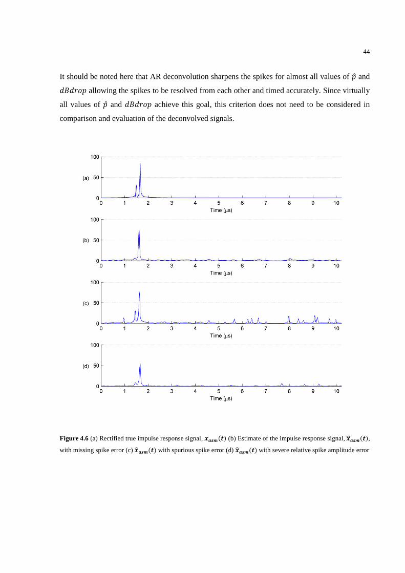
44
It should be noted here that AR deconvolution sharpens the spikes for almost all values of �̂ and ������ allowing the spikes to be resolved from each other and timed accurately. Since virtually
all values of �̂ and ������ achieve this goal, this criterion does not need to be considered in
comparison and evaluation of the deconvolved signals.
Figure 4.6 (a) Rectified true impulse response signal, |���(z) (b) Estimate of the impulse response signal,|:���(z), with missing spike error (c) |:���(z) with spurious spike error (d) |:���(z) with severe relative spike amplitude error

45
1) No Missing Spikes: This is a very important feature for an enhanced signal. A lost spike
means that the operator will not see a defect indication and the defect will be missed. This may
result in accepting a flawed weld and therefore it is critical to avoid this type of error in our
estimate, x����(t), of the deconvolved signal. A missed spike error usually occurs when an
excessively low AR order number �̂is used; this makes the model too simple to incorporate the
subtle perturbations caused to the overall measured signal, �(�), by the small spike. Figure 4.6b
shows an AR deconvolved signal obtained with an excessively low value of �̂; a comparison
between this signal and the impulse response signal (Figure 4.6a) shows that the small spike,
which corresponds to the crack tip echo, is missing and is not recovered by the AR
deconvolution.
2) No Extra Spurious Spikes: Spurious spikes usually appear when we use a value for �̂ that is
too high. Using a high AR order value lowers the chance of missing spikes but it also induces the
AR model to “follow” (model) individual random noise fluctuations as if they were true flaw
indications; this can lead to a relatively large spurious spike which can be misinterpreted as a real
flaw indication by the operator and may result in rejecting a good weld. This then leads to extra
weld repair costs; therefore, this type of error should also be avoided. Figure 4.6c shows a
deconvolved signal that is obtained using an excessively high AR order �̂.
3) No Mislocated Spikes: The sizing of the cracks is done using spike arrival time
measurements via the time-of-flight-diffraction (TOFD) method. Therefore, sizing accuracy
depends directly on the correct placement of the ultrasonic echoes in the time domain. The AR
deconvolution method can have two types of error in timing of the spikes: the first one is a
general lag in which all spikes are time-shifted together by the same amount. This error does not
affect the sizing accuracy since TOFD is dependent on the relative time between the spikes and
not the absolute arrival times, hence this error type can be neglected. The second error type
however, is the error in relative temporal positions of the spikes and should be avoided since it
directly affects the sizing accuracy. In section 4.2.2, we will show how to distinguish these two
error types when evaluating the performance of a signal processing technique.
4) Correct Spike Amplitude Estimation: Although amplitudes of the spikes are not used in the
sizing of the cracks in the TOFD method, correct amplitude values help the operator interpret the
overall ultrasonic map of flaw echoes. In addition, in cases where a number of A-scans are

46
stacked together in a B-scan or C-scan display, large random errors in echo amplitudes will result
in inconsistencies between the adjacent A-scans and will smear the final image, making it harder
to interpret. Figure 4.6d shows a signal with incorrect spike amplitudes.
5) Low Noise: Low noise in a signal makes the detection and interpretation of the defect
indications easier and enables the operator to make a more accurate interpretation of the signal.
4.2.2 The Figure of Merit
Now that we have established what features to look for in our estimate of the impulse response
signal, ��(�), we can define a quantitative measure for its “merit”. One major advantage of
working with synthetic signals is that we have access to the true impulse response, �(�), of the
system – this would represent a 100% merit score if one could perfectly recover this ideal
response through signal processing of the measured ultrasonic signal, �(�). We need to find a
quantitative way to compare ��(�) with the true impulse response, �(�), in a manner that focuses
on the key features described in Section 4.2.1.
A common way of measuring the similarity of two signals is to use a norm of the difference ,(�)between the analytic signal magnitude (asm) of the two signals, which we call the residue
signal:
,(�) = �� ��(�) − � ��(�) ( 4.5)
An issue with this residue signal is that it is very sensitive to a general lag error, whereby one
signal is time-shifted relative to the other. As described in the previous section, such a
generalized time shift would not affect our estimate of the time difference between any two
echoes, and would therefore not affect our estimate of crack size. Therefore, one should not
assign a high cost to such a shift, although it would significantly affect our calculation of the
residue according to Equation ( 4.5).
To overcome this problem we need to "align" the �� �� and � �� signals before computing the
residue signal. For signal alignment, we calculate the cross correlation function of � �� and �� �� to find the lag value for which the cross correlation is a maximum, and then shift the �� ��
by this lag value to temporally align the two signals. We can then calculate the corrected residue

47
signal by Equation ( 4.5) using the time-shifted �� ��. Although this sequence of operations may
appear to be slow and cumbersome, it is important to note that these operations are being used
only to develop the signal processing algorithm that will ultimately see field use.
In order to be able to compare the deconvolved signals, a single “cost” value must be assigned to
the residue signal, ,(�). This can be achieved by applying a norm to the residue signal. The most
common norm, usually used to evaluate the "energy" of a signal, is the L2 norm.
Γ = ‖,(�)‖7 = �e,7�_7 ( 4.6)
This indicator, however, is overly sensitive to the amplitudes of the major signal peaks, even
though signal amplitudes are not of prime importance in TOFD assessments of crack size. A
more suitable choice is the relative L2 norm of the error signal, Ψ, which normalizes each error
residue by the amplitude of true signal. This indicator places increased emphasis on amplitude
variations in smaller spikes (i.e., increased sensitivity to extra small spurious spikes) and de-
emphasizes the absolute errors in large spike amplitudes:
Ψ = �e ,7� �� + 67�_7 ( 4.7)
where 67 is a noise desensitizing factor used to prevent instabilities in cases where � ��
approaches zero. To evaluate the performance of Ψ, we can use Table 4.1. This table shows in a
qualitative sense the sensitivity of various error norms to deficiencies in our enhanced signal
response �� ��.
Error Type Missing Spikes Spurious Spikes Mislocated Spikes Amplitude Error Noise
Ψ = �e e7x��� + q7�_7 Very Low High High Low High
Φ = �e e7x���� + q7�_7 Vey High Low High Low Low
Table 4.1 Cost assignment of error functions of two error norms, ¢ and £, to different error types.

48
As we can see in this table, Ψ assigns a high cost to spurious spikes, mislocated spikes and noise,
and a relatively low cost to amplitude error. These are desirable features for a norm; however, it
does not assign a sufficiently high cost to missing spikes - one of the most important errors. To
overcome this problem, we define another relative L2 norm to perform the normalization
operation relative to the estimated signal, �� ��, instead of the true signal, � ��:
Φ = �e ,7x���� + 67�_7 ( 4.8)
where 67 is again a noise desensitizing factor. As seen in Table 4.1, this indicator assigns a very
high cost to missing spikes and is a suitable complement to the first indicator Ψ. Based on a
number of trials, it was determined that an optimal cost function can be achieved by combining
these two indicators :
Υ = Ψ+ QΦ ( 4.9)
where Q is a weighting factor that indicates the relative importance of not having missing spikes.
An appropriate choice for µ could depend on the particular ultrasonic testing job at hand. We
used a Q value of 0.1 based on ultrasonic inspection trials of simulated pipeline girth welds.
Finally, we use this cost function Υ to define a normalized figure of merit ��� as follows:
FOM = (1 − ΥΥs) × 100 ( 4.10)
where Υs is the cost function for an estimated signal, �� ��(�), identically equal to zero. An
estimated impulse response signal, �� ��(�), with an ��� of 0% has the same (poor) merit as a
zero signal, and an estimated impulse response signal, �� ��(�), with an ��� of 100% would be
equivalent to the true impulse response signal, � ��(�).

49
4.3 Synthetic Signal Data Analysis
In Section 4.1, we generated a large dataset of synthetic signals with various spike train
configurations and noise levels. In this section, we use the AR deconvolution method described
in Chapter 3 to enhance these synthetically generated signals with various values of �̂ and ������. We then use the figure of merit introduced in Section 4.2 to compare the relative merit
of the enhanced signals as functions of background noise levels. Analysis of those results allows
us to develop an algorithm for finding the optimum values for �̂ and ������ as functions of
noise levels, to yield the highest final figure of merit.
In the first step, we apply the AR algorithm to all of the signals in the raw dataset generated in
Section 4.1 (Equation ( 4.4)). The generated raw dataset is a matrix of 4800 signals, consisting of
12 impulse response (IR) signals, each with 40 different ��� levels, with 10 realizations of each
IR signal at each ���.
< �"9)"�"�,� >= [��� ×��o� × ��K �*� �*�J�] ( 4.11)
Each of these 4800 signals is then processed by the AR algorithm using both fitting methods
(Burg and modified covariance) and a wide range of values of ������ and �̂ in order to evaluate
the influence of these parameters on the merit of the resultant �� ��(�). For this investigation, we used 45 values for the parameter ������ ranging from 3dB to 12dB
with increments of 0.2dB. For each value of ������ we used 30 values for the normalized AR
order �̂ , for the modified covariance fitting method, the values ranged from 0.05 up to 0.65, and
for the Burg fitting method, they ranged from 0.05 up to 0.95. The processed dataset matrix
therefore has about 13 million enhanced signals, where
< ¤�ℎ"�%,�)"�"�,� >= [��� ×��o� ×��K �*� �*�J� × �¥�¥¦��� × ��� × �§*��*J¨©K�ª�¥] ( 4.12)
The figure of merit defined in Equation ( 4.10) was then used to evaluate the merit of each
processed signal, �� ��(�), compared to its corresponding rectified true impulse response signal, � ��(�). This yielded a data matrix containing the ��� value for each enhanced signal. ���
values were averaged over the 10 realizations of each signal and 12 signal types to reduce the
dataset to a more manageable level for observing general trends, and to reduce the effects of

50
random noise fluctuations on determining general signal trends. This yielded an averaged ���
data matrix of the following magnitude:
< «¬,�",��� >= [��o� ×�¥�¥¦��� ×��� × �§*��*J¨©K�ª�¥] ( 4.13)
This average ��� matrix, containing approximately 100,000 data points, effectively allows us
to express the FOM as a function of SNR, dBdrop, and �̂. In the following section, we use this
information to extract trends and find optimum values for ������ and �̂ as a function of ���.
4.3.1 Optimizing AR Model Order �̂ and ������
The data showing the dependence of the ��� as a function of ���, ������ and �̂, enables us
to find the optimum values of ������ and �̂ corresponding to any given value of ��� , i.e.,
values for ������ and �̂for which we get the highest value of ���. In mathematical form, we
have:
���������(���), �̂���(���) = "�S"�¥�¥¦��,�����(���, ������, �̂) ( 4.14)
By repeating this process for a wide range of ��� values, we can generate plots of ��������� and ���� versus ��� as shown in Figure 4.7.
The uncertainty bars corresponding to each ��� value show the acceptable range of values of �̂
and dBdrop to get an optimal enhanced signal. Within these uncertainty bars, the ��� is more
than 99% of its maximum value at that ���. It can be seen in Figure 4.7 that the error bars
become larger as the ��� increases; this shows that at higher ��� values the enhanced signal
quality is relatively insensitive to the exact choice of �̂ and ������. By contrast, at low SNR
values, the signal enhancement performance drops quickly as we deviate from the optimal
choices of these two parameters.

51
Figure 4.7 Optimum ®¯®°±² and ²: versus ³´µ for both Burg and Modified Covariance methods
This point is better illustrated in Figure 4.8 by contours on the �̂ − ������ plane (which is
plotted using Burg method data). Inside each contour corresponding to three SNR values, the
solution is acceptable, according to the criterion used for determining error bars in Figure 4.7. As
the ��� is decreased, the contours become smaller; this indicates that the results are becoming
more sensitive to the choice of �̂ and ������. In addition, the contours move toward lower �̂
and ������ values as the SNR decreases; this trend was expected since at low ��� the useful
signal bandwidth of a signal is generally smaller such that a small value of dBdrop is appropriate
for signal processing. In addition, the AR technique becomes increasingly sensitive to noise as
the value of �̂ is increased, such that a low �̂value is optimal for noisy signals. Similar trends

52
were observed when using modified covariance method; however, those contours are not shown
in Figure 4.8 to maintain clarity of the figure.
Figure 4.8 Acceptable ¶·¸ regions for three ³´µ levels (using Burg method)
Under field conditions, the SNR of a measurement system can be readily measured, but there
will be no other a priori information generally available when acquiring and processing an
ultrasonic echo signal. Therefore, we need to be able to find the optimum values for �̂ and ������ based solely on the signal's ���. This task can be achieved most simply by fitting a
straight line approximation to the data of Figure 4.7, as demonstrated in the following section.
Fitting Algorithm
One method of fitting a line to the data of Figure 4.7 is to ignore the error bands and only use the
optimum values (designated by “x”) at each ��� and fit a line by a regular linear regression
technique. A linear regression fit, however, is based on the assumption that the data points are
samples from a Gaussian distribution and uses the L2 norm as the cost function to find the best
fit to the data. Such a routine does not take into account that the cost function (the inverse of ���) is different for each ��� value, which is evident from the asymmetrical error bars with

53
variable widths in Figure 4.7. Therefore, using linear regression may not be the optimal route for
fitting a straight line to the data.
A superior approach is to choose the line that yields the highest sum of ��� over the range of ��� values. Since we have the ��� values for all ������'s or �̂'s at each ��� we can
optimize the parameters (slope ("�*JK) and intercept ($�*JK)) of the line ("�*JK × ��� + $�*JK) to
get the highest sum of ��� over all ��� values. In mathematical notation, we will have:
"¥�¥¦�� , $¥�¥¦�� = "�S"� ¹v¹º»¼,½¹v¹º»¼{ e ���(���* , "¥�¥¦�� × ���* + $¥�¥¦��¿ÀÁÂ
Ãg_ , �̂���(���*))} ( 4.15)
"��, $�� = "�S"� ¼: ,½¼:{ e ���Z���* , ���������(���*), "�� × ���* + $��^¿ÀÁÂ
Ãg_ } ( 4.16)
We used a brute force, trial and error approach to find the optimum line parameters according to
Equations ( 4.15) and ( 4.16). For the Burg method dataset, we obtained the following results:
Å"¥�¥¦�� = 0.23$¥�¥¦�� = 0.79� ⇒ ��������� = 0.23 × ��� + 0.79 ( 4.17)
Å"�� = 0.014$�� = 0.21 � ⇒ �̂��� = 0.014 × ��� + 0.21 ( 4.18)
We can use these two equations to find ��������� and ���� for all ��� values between 15dB
and 25dB for performing the AR deconvolution (with Burg as the fitting method). Figure 4.9
shows the fitted lines on the datasets.
Similarly for the modified covariance method, the corresponding relationships for �̂��� and
��������� were calculated as follows:
Å��������� = 0.25 × ��� + 0.74�̂��� = 0.012 × ��� + 0.15 � ( 4.19)

54
Figure 4.9 Optimum ®¯®°±² and ²: versus ³´µ with fitted lines for the Burg method
4.3.2 Burg vs. Modified Covariance
In Section 3.4, we compared general features of the two AR model fitting methods: Burg and
modified covariance. To summarize, the modified covariance method is slower than the Burg
method and it does not guarantee stability of the algorithm; therefore, an additional step is
required to achieve stability; which adds complexity to the algorithm. The covariance method,
however, is not prone to the spike splitting problem experienced with the Burg method.
Furthermore, in low noise conditions, we qualitatively showed that the covariance method is

55
superior to Burg in recovering the impulse response signal. In this section, a quantitative
comparison of results obtained from the Burg and covariance methods is carried out.
In Equation ( 4.13) we obtained the ��� of both the Burg and modified covariance method as a
function of ���, ������ and �̂ for our sample dataset. We now compare the performance of the
two algorithms based on the optimum choice for ������ and �̂ values for the two respective
methods, i.e., using the maximum ��� value corresponding to each ���. Figure 4.7 shows the
maximum ��� for the two methods.
Figure 4.10 Figure Of Merit (¶·¸) achieved by Burg and modified covariance methods as a function of signal-to-
noise ratio (³´µ). Optimal values of ² and ®¯®°±² were used to calculate the FOM for each method.
As can be seen in Figure 4.7, the modified covariance method performs slightly better than the
Burg method at high ��� values but their performance is similar for medium and low noise
conditions. The slight advantage seen with the modified covariance method does not justify its
higher computational complexity, lower speed, and poorer stability; therefore, the Burg method
is the preferred choice based on this dataset of synthetic signals. The data obtained using the
modified covariance method will still be presented in the following sections for comparison.

56
4.3.3 Dependence of AR Model Order on the Number of Data Points
Previous researchers [22] proposed that the optimum AR order number ���� is linearly
proportional to the number of data points in the bandwidth window, ���. Based on this
assumption, we normalized � by ��� in Section 3.3 and defined a more general AR order
number, �̂ = �ovw. This new variable makes �̂��� independent of the number of points in the
bandwidth window. In this section we quantitatively examine our assumption of linear
correlation between ���� and ���.
To this end, we add a new dimension to the raw dataset as defined in ( 4.11), in order to
investigate the influence of ��� on ����. In this dimension, we vary the number of signal data
points in the time domain from 512 to 1512 with 100-point increments. By increasing the signal
length, we get increasing ��� corresponding to a fixed ������. The expanded raw dataset now
has the following number of signals:
< �"9)"�"�,� >= [�ovw × ��� × ��o� × ��K �*� �*�J�] ( 4.20)
The signals in this dataset are then deconvolved in a similar process to that described in Section
4.3. To keep the dataset size manageable, the number of ��� values is decreased from 40 to 10,
and a single ������ value (5dB) is used. Each signal in the raw dataset is processed using the
AR deconvolution method with various AR order numbers and both the Burg and covariance
fitting methods. This results in the following dataset:
EnhancedDataset = [�ovw ×�ЦÑK�*¨J �� × ��o� × ��K �*� �*�J� × �� ×�§*��*J¨©K�ª�¥] ( 4.21)
Using this dataset, in the same process described earlier in Section 4.3, the ��� matrix is
created by computing the ��� for each signal in the enhanced dataset. This ��� matrix is then
averaged over the signal realization and impulse response dimensions (see Equation ( 4.13)).
Based on this matrix, the optimum AR order, ����, for each ���, ���, and fitting method (Burg
or modified covariance) is calculated by finding the AR order number which maximizes the
averaged ��� (see Equation ( 4.14)):
< ���� >= [�§*��*J¨©K�ª�¥ ×��o� × �ovw] ( 4.22)

57
Figure 4.11 shows how ���� varies with ��� at a single ��� (20dB) for both Burg and modified
covariance fitting methods.
Figure 4.11 Optimum AR order ²±²z as a function of number of data points in the Bandwidth Window (´¯Ò) at
³´µ = ÓÔ®¯ for both Burg and modified covariance methods. Lines with zero intercepts are fitted to the data
points to evaluate the validity of the relationship ²±²z = ²:±²z × ´¯Ò.
The linear correlation is evident from both curves in Figure 4.11. A more quantitative evaluation
can be carried out by calculating the coefficient of determination (R-squared) value for fitting a
line with zero intercept (representing the relationship ���� = �̂��� × ���) to the data at each
��� value. For ���=20dB, which is the data shown in Figure 4.11, the R-squared values are 0.8
and 0.9 for Burg and modified covariance methods respectively; similar results were obtained at
other ��� values. The averages of R-squared values calculated at all ��� values, were found to
be 0.80 and 0.85 for Burg and modified covariance respectively - these high values indicate a
good linear fit. This shows that once �̂��� has been calculated for one signal length, ���� can be
found with good accuracy by the following relationship:
���� = �̂��� × ��� ( 4.23)

58
4.4 Final Optimized Algorithm
In Chapters 3 and 4, we investigated and optimized various steps of the autoregressive
deconvolution method. In this section, we summarize the steps and present the flowchart for the
final optimized algorithm.
Preliminary Deconvolution
1) Calculate Õ(�) and Ö(�), the discrete Fourier transforms of �(�) and ℎ(�), where y(n) is the
measured NDE signal, and h(n) is the reference echo.
2) Calculate an estimate of the discrete Fourier transform of the impulse response signal by
standard deconvolution, ×Ø(�) = Õ(�)Ö(�) (Section 3.1).
Parameter Selection
3) Estimate the ³´µ of the measured signal �(�) according to Equation ( 4.3), using a segment
of �(�) where there are no flaw echoes (Section 4.3.1).
4) Find ®¯®°±²±²z according to this ��� value using Equation ( 4.17).
5) Use the optimum ������ calculated in step 4 and the reference echo signal ℎ(�) to find the
Bandwidth Window according to the dBdrop method described in Section 3.2.
6) Find the optimum normalized AR order, ²:±²z, at the ��� value calculated in step 3, using
Equation ( 4.18).
7) Using the bandwidth window calculated in step 5 and optimum normalized AR order, ²:±²z, calculated in step 6, calculate the optimum AR order ²±²z according to Equation ( 4.23).
AR Modeling and Extrapolation
8) Apply the bandwidth window calculated in step 5 to the deconvolved signal ;<(�) obtained in
step 2.

59
9) Use the Burg method to fit an AR model to the ;<(�) data points that lie within the bandwidth
window.
10) Use the AR model to extrapolate the ;<(�) data points that lie within the bandwidth window
to higher and lower frequencies (see Section 2.6.2).
Transforming to Time Domain and Rectification
11) Set the negative frequency values of ;<(�) equal to the complex conjugate of the positive
values.
12) Apply an inverse discrete Fourier transform to ;<(�) to obtain the estimated impulse response
signal in time domain, |:(�). 11) Apply the analytic signal magnitude method to ��(�) to obtain the final rectified estimated
impulse response signal |:���(�) (see Section 3.5).
Note that the analytic signal magnitude can also be applied directly to the ;<(�) data at step 10.
Figure 4.12 shows a flowchart of the optimized AR deconvolution algorithm. In the next chapter,
we apply this final AR deconvolution algorithm on experimental signals to evaluate its
performance.

60
Figure 4.12 Flowchart of the optimized AR deconvolution algorithm

61
Chapter 5
5 Experimental Results and Discussion
In the previous chapter, we developed a method for choosing the parameters �̂ and ������ for
AR deconvolution of an ultrasonic echo signal, based on its signal-to-noise ratio. This method,
however, was developed and evaluated on the basis of synthetic signals; even though an attempt
was made to mimic real ultrasonic echo signals to the extent possible, there are some features of
real signals that may have been inadequately represented in that development exercise. One of
these features is the grain noise, which originates from waves scattering off grain boundaries of a
granular material – this noise would not have the flat spectral shape we assumed when we added
synthetic white noise in our optimization studies.
Another feature of a real echo signal which distinguishes it from our synthetically generated
signals is the imperfect reflection of waves by cracks: In our synthetic signals, we assumed that
all echoes have the same spectral content (that of the reference echo) and vary only in amplitude
and timing. This, however, is not always exactly true in real signals. For example, a crack tip
diffracted echo will have a different frequency content than a specularly reflected signal, such as
from a corner trap or a flat surface. These deviations from the ideal situation introduce error into
the deconvolution process.
In this section, we evaluate the performance of the optimized AR deconvolution method when
applied to real ultrasonic echo signals. The real signals are obtained through two experiments:
The first experiment is the inspection of a welded joint between two plates, where the weld
contains embedded shallow root cracks; this shows the performance of the technique in detecting
and sizing small cracks. The second experiment is the inspection of an austenitic weld with large
grain structure, and shows the performance of the technique in the presence of significant grain
noise.

62
5.1 Shallow Root Cracks in a Butt Weld
In this section, we inspect a butt-weld with shallow root cracks using a phased array system. The
test piece is manufactured by Sonaspection (Concord, NC) and contains six shallow root cracks
of various depths embedded along the welded joint of two, 12.4mm thick, carbon steel plates.
The weld cap was ground off so that the ultrasonic inspection wedge could be put closer to the
weld centerline. This test piece can be seen in Figure 5.1.
Figure 5.1 A schematic of flaw locations and length overlaid on the figure of the test plate. Flaws 1 to 6 are
nominally 0.5, 0.75, 1, 2, 3 and 5mm deep root-breaking cracks respectively. The lengths and locations of these
cracks are shown in the figure.
5.1.1 Data Acquisition Setup
The first steps in ultrasonic inspection of a weld are to specify and configure the required
equipment and to devise a scan plan to detect and size the flaws. Usually, ray-tracing software is
used for designing a scan plan. This software visualizes the beam path through the wedge and the
test piece and helps in selecting scan parameters such as the number of ultrasonic beams needed
to span the weld, the beam angles, wedge position with respect to the weld, etc. It also makes the
interpretation of the scan results easier, since we can simulate each beam path using the software
and find the origin (flaw location) corresponding to each received echo.
The inspection equipment can be divided into two groups: The first group is the ultrasonic
equipment, which includes the phased array probes, the wedges and the pulser/receiver. The

63
second group is the motion equipment, which controls how the probes and wedges are mounted
and moved along the weld.
Ultrasonic Equipment: In this test, we used a 5MHz phased array probe with 16 elements,
model 5L16 manufactured by Olympus NDT Canada (Quebec, QC). The probe was mounted on
a shear wedge, Olympus model SA2-N55S, which refracts the ultrasonic beam to a 55-degree
shear wave in steel. Shear wave beams at other angles (from about 35 to 75 degrees) can be
generated by steering the phased array probe beam, via adjustment of the relative time delays
among the array elements. An Olympus Omniscan phased array system was used as the
pulser/receiver and data acquisition unit. Figure 5.2 shows this setup.
Figure 5.2 Experiment setup for scanning the plate. 1) Sonaspection plate with embedded flaws 2) Phased array
probe 3) Motion system with a rotary encoder 4) Phased array unit (pulser/receiver)
Motion Equipment: A manual locomotion system designed by Eclipse Scientific (Waterloo,
ON) was used for this experiment. The unit contains fixtures to hold the welded plate in place,
and it has a moving arm where the wedge can be mounted and moved along the weld. The arm
also has a rotary encoder to record the position of the wedge (See Figure 5.2). This setup allows
data to be captured in a reliable and reproducible manner by fixing the position of the wedge
with respect to the weld line and recording the probe position along the weld using the attached
encoder.
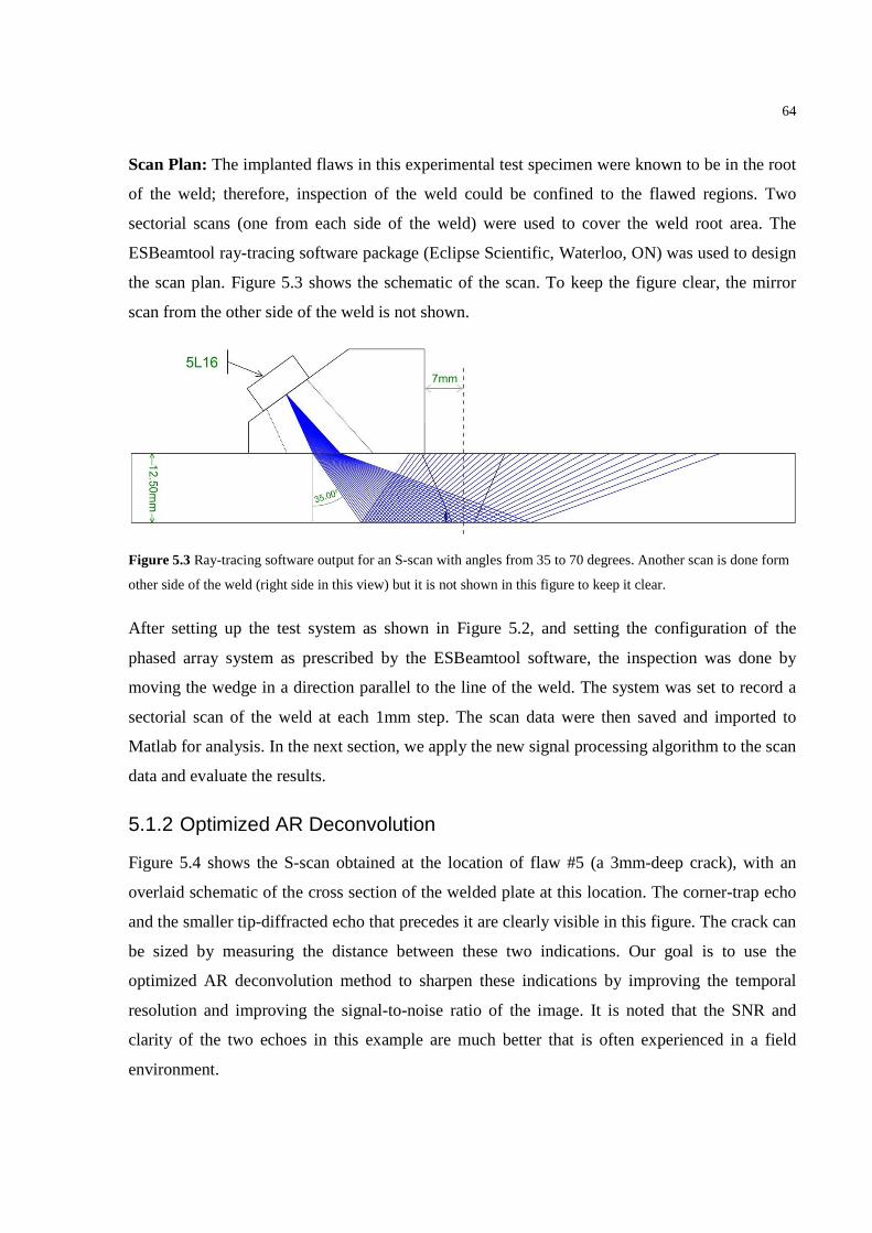
64
Scan Plan: The implanted flaws in this experimental test specimen were known to be in the root
of the weld; therefore, inspection of the weld could be confined to the flawed regions. Two
sectorial scans (one from each side of the weld) were used to cover the weld root area. The
ESBeamtool ray-tracing software package (Eclipse Scientific, Waterloo, ON) was used to design
the scan plan. Figure 5.3 shows the schematic of the scan. To keep the figure clear, the mirror
scan from the other side of the weld is not shown.
Figure 5.3 Ray-tracing software output for an S-scan with angles from 35 to 70 degrees. Another scan is done form
other side of the weld (right side in this view) but it is not shown in this figure to keep it clear.
After setting up the test system as shown in Figure 5.2, and setting the configuration of the
phased array system as prescribed by the ESBeamtool software, the inspection was done by
moving the wedge in a direction parallel to the line of the weld. The system was set to record a
sectorial scan of the weld at each 1mm step. The scan data were then saved and imported to
Matlab for analysis. In the next section, we apply the new signal processing algorithm to the scan
data and evaluate the results.
5.1.2 Optimized AR Deconvolution
Figure 5.4 shows the S-scan obtained at the location of flaw #5 (a 3mm-deep crack), with an
overlaid schematic of the cross section of the welded plate at this location. The corner-trap echo
and the smaller tip-diffracted echo that precedes it are clearly visible in this figure. The crack can
be sized by measuring the distance between these two indications. Our goal is to use the
optimized AR deconvolution method to sharpen these indications by improving the temporal
resolution and improving the signal-to-noise ratio of the image. It is noted that the SNR and
clarity of the two echoes in this example are much better that is often experienced in a field
environment.

65
Figure 5.4 The S-scan of the fifth flaw (3mm high crack) at the scan location of 211mm. The piece schematic is
overlaid on top of the S-scan to make the interpretation easier. Note the difference between the sound beam path in
the material and the displayed path in the S-scan. Where S-scan beams seem to exit the part at the bottom face of the
specimen, they are in fact reflected back up inside the piece. This is shown in the figure by comparison of a single
beam path in the S-scan and in the actual piece. The corner-trapped echo and tip echoes are visible in the S-scan.
In order to apply the optimized AR deconvolution method, a reference echo and an estimate of
the ��� in each of the A-scans that constitute the 2-D S-Scan are required. The reference echo
can be obtained using an International Institute of Welding (IIW) type calibration block (Figure
5.6). This calibration block is designed by the International Institute of Welding and is used by
ultrasonic NDT technicians to calibrate their ultrasonic equipment. We use the same ultrasonic
equipment and setup as employed in the scan of the test specimen to acquire a reference
reflection echo from the curved portion of the calibration block. The resulting S-scan can be
deconstructed to yield a reference echo A-scan corresponding to each beam angle. These A-scans
are similar but not identical to each other; for simplicity, we used the 45-degree A-scan as our
reference echo to deconvolve all of our experimental echo signals from the welded plate.

66
Figure 5.5 The International Institute of Welding (IIW) type calibration block with overlaid schematic of the probe
and beam paths used in the experiment. The probe position on the calibration block is adjusted to set the exit point
(the location at which the beam exits the wedge and enters the piece) of the 45 degrees beam at the center of the
curvature of the curved portion of the block. This results in a clean reference signal at 45 degrees by focusing the
reflected beams straight back at the probe.
The SNR of each A-scan that together constitute the S-scans captured from the welded plate can
be calculated according to Equation 4.3. For this equation, the maximum amplitude of the signal
and the standard deviation of noise are required. The maximum amplitude can be readily
measured from each A-scan signal; the noise standard deviation can also be estimated using the
method described in Chapter 4. In this method, a region in the A-scan where there are no flaw
echoes or geometric reflectors is selected, such that only signal's noise is present in that region.
The standard deviation of the signal from that region is then calculated, and is used as an
estimate of the noise standard deviation of the entire A-scan. The SNR then can be calculated for
each A-scan that makes up the S-scan using Equation 4.3.
Knowing the reference echo and SNR of each A-scan, we can apply the AR deconvolution
algorithm to all A-scans and generate an enhanced S-scan. Figure 5.6 shows the S-scan at the
location of the 3mm crack (scan position of 211mm along the weld), before and after applying
the AR deconvolution. Results from both the Burg and modified covariance fitting methods are
presented.

67
(a)
(b)
(c)
Figure 5.6 (right column) The S-scans of the 3mm deep crack at the scan location of 211mm. (left column)
The A-scans corresponding to the beam at location of the blue line on the S-scan. (a) The original S-scan (b)
Enhanced S-scan using optimized AR deconvolution with the Burg method. (c) Enhanced S-scan using
optimized AR deconvolution with the modified covariance method. Note that the signal processing system
makes it easier to resolve two closely spaced echoes, and determine accurately the time difference between
them.

68
We can see that for both fitting methods, echo peaks are sharpened, and the image looks more
clear compared to the unprocessed signal (the peak amplitudes of both S-scans are equal). To
further investigate the enhancement, the A-scans for two beams at 62 and 58 degrees are
extracted from these S-scans and displayed in Figure 5.7a and Figure 5.7b respectively.
(a)
(b)
Figure 5.7 The original and enhanced (by Burg and modified covariance methods) A-scans from the S-scan of the
3mm deep crack at the scan location of 211mm. (a) A-scans at 62 degrees (b) A-scans at 58 degrees. Two spurious
spikes are generated in the enhanced A-scan when using the modified covariance fitting method and the crack-
diffracted peak is missing.
As can be seen in Figure 5.7a, the enhanced A-scans have sharper spikes and the resolution is
increased with both the Burg and modified covariance methods for determining the extrapolation
coefficients, "* 's. In order to evaluate the resolution enhancement in a quantitative way, a figure-
of-merit for resolution improvement is required. One suitable figure of merit is the Full-Width at
Half-Maximum (FWHM) of a spike, which is the width of the spike at half of its maximum
value. In the data set of this experiment, the optimized AR deconvolution reduced the FWHM of
the spikes by about 80% by both deconvolution methods, and provides little guidance on which
of the two signal processing methods is superior.
Spurious spikes

69
Figure 5.7b shows the original and enhanced A-scans at 58 degrees. Similar to the 62 degrees A-
scan in Figure 5.7a, a substantial reduction in FWHM is achieved. However, the modified
covariance method has generated two spurious spikes, and omitted the crack tip-diffracted echo
of interest. It should be noted here that the Burg method is also susceptible to spurious spike
error, but in this experiment data set, the modified covariance was found more vulnerable to this
type of error.
We showed that the AR deconvolution is capable of reducing FWHM. In order to show how this
reduction affects the crack sizing error, we investigate the sizing estimate of a root-breaking
crack achieved by backscatter diffraction using a single A-scan, as was described in Chapter 2
(See Figure 2.9). Assuming that the tip and corner-trapped echoes arrive at times �_ and �7, the
apparent crack depth 51+ can be calculated as 51+ = %(�7 − �_)/2 where % is the speed of wave
propagation. The actual crack depth 51 can then be calculated using Equation 2.1, which is
repeated here:
51 = 5� −UV 5�cos(R) − 51+Y7 − Z5� tan(R)^7 ( 5.1)
Assuming that the wall thickness 5�, beam angle R and wave propagation speed % can be
measured accurately and their error is negligible, using error propagation rules we will have:
Δ51 = Ù51Ù51+ Δ51+ = Ù51Ù51+ c2Ú(Δt7)7 + (Δt_)7 ( 5.2)
where Δ�_ and Δ�7 are errors in measuring �_ and �7 respectively. If we assume that the error in
measuring arrival times of spikes is proportional to the FWHM of the signal, the 80% reduction
in the FWHM will change the sizing error as follows:
(Δ51)¥K1�JÛ��ÛK¥ = Ù51Ù51+ c2Ú(0.2Δt7)7 + (0.2Δt_)7 = 0.2(Δ51)¦ Ü ( 5.3)
This shows, in theory, that the sizing error (uncertainty) of the cracks drops by 80%. As a
numerical example, consider the inspection of a 3mm crack at the root of a weld in a 20mm thick
pipe, using a 60 degree 5MHz compression wave (with a speed of 5.9SS/Q�). We assume that
the uncertainty in measuring the arrival times (Δ�_ and Δ�7), can roughly be approximated by

70
half of the FWHM of an echo spike. For a typical 5MHz transducer, this is about 0.1Q�.
Substituting these values into Equation 5.2 we find Δ51 ≅ 1SS. According to equation 5.3, this
uncertainty in crack size drops to Δ51 ≅ 0.2SS after the deconvolution.
Using a similar calculation, it can be shown that the size of the smallest sizable crack (17 Ý�ÞiÝ��7 ),
for which the tip and corner-trapped echoes can be resolved, is also lowered by 80%. It should be
noted here that these calculations only take into account the error originating from uncertainty in
locating the arrival time of a spike by the operator; there may be other sources of error such as
improper calibration of the equipment, a poorly-performing transducer, or wall thickness that
deviates from its specifications. In addition, the precision and accuracy of the spike positions
after applying optimized AR deconvolution needs to be measured using a set of controlled
experiments. This would require destructive measurements of precise defect sizes, and is beyond
the scope of this project.
To this point, we have shown that enhanced AR deconvolution is capable of sharpening
(narrowing) reflection echo “spikes” and thereby improving their theoretical temporal resolution
capability; however, in the experimental S-scans we investigated so far in this chapter, there
were no overlapping echoes. In order to evaluate the performance of the technique on resolving
overlapping echoes, we move to smaller surface-breaking cracks. Figure 5.9a shows an S-scan at
the location of a small crack (nominal depth of 0.5 mm) with two overlapping echoes from the
crack tip and bottom corner. Figure 5.9b shows an enlarged view of the boxed area. Only one
echo can be distinguished at this level. The AR deconvolved S-scan (using the Burg fitting
method) is displayed in Figure 5.9c; two indications are resolved in this figure.
There are two issues for crack sizing using this deconvolved S-scan. The first issue is the low
lateral resolution (the step in angle change), which causes detached indications on each A-scan
and makes the picture "pixelated" in the lateral dimension as can be seen in Figure 5.9c. This
problem can be solved by increasing the lateral resolution in the scanning operation (by
decreasing the size of the angle step); however, the equipment capabilities and data storage
issues may limit this option.

71
The second issue is the significant amplitude errors in the corner-trapped and tip diffracted echo
spikes (particularly the latter), which might confuse the inspector performing the test, in finding
the location of the peak amplitude.
These issues make it hard to locate an accurate position for top and bottom of the crack and
hence hinder the sizing of the crack. We can however use the method described in Chapter 2 for
sizing the cracks using a single A-scan (for which we do not need to be concerned with
amplitude deviations compared to other A-Scans) to find the crack size. The 49 degrees A-scan,
which has the spike with the maximum amplitude, is chosen to size the crack. Figure 5.8 shows
this A-scan.
Figure 5.8 The 49 degrees deconvolved A-scan. The time difference between the tip and corner-trapped echo is
measured to be 0.1±0.03 microseconds.
The apparent crack depth, 51+ , is calculated to be 0.16mm (51+ = 1(��f�Þ)7 ). The plate thickness at
the location of this beam, 5�, is measured to be 13.1mm. By substituting these values along with
the beam angle R=49 in Equation 5.1, the estimated crack depth is found to be 0.3 ± 0.1mm,
which is barely within the 0.5±0.25mm reported crack length in the as-built spec sheet of the test
piece. The under- estimation of the crack size can be due to uncertainty in manufacturing of the
crack, or error in the sizing technique. The manufacturer (Sonaspection) had issued a caution that
it was difficult for them to control the size of very shallow cracks. A full set of destructive tests
is needed to evaluate the overall accuracy of the sizing method.

72
(a)
(b)
(c)
Figure 5.9 (a) The S-scan of the nominal 0.5mm high crack at the scan location of 9mm. The box shows the area
of interest. (b) Magnified portion of the Figure 5.7a inside the area of interest. (c) Enhanced S-scan of the
magnified portion of the S-scan using the optimized AR deconvolution with burg as the fitting method. Since the
lateral resolution is low, the imaging interpolation scheme is unable to merge adjacent A-scans efficiently and the
picture has become laterally "pixelated".
Detached Indications

73
5.2 Flat Bottom Holes in an Austenitic Weld
This test was carried out as a part of technique development for automated inspection of
austenitic welds in clad pipes. The test piece was a 12-inch outer diameter clad pipe made from
carbon steel, with a 3mm thick layer of corrosion resistant alloy explosively welded to the inside.
This type of material cannot be welded using normal weld filler materials and special fillers such
as an Inconel alloy or stainless steel must be used. Inspection of such welds is challenging since
they have large grains that scatter the ultrasonic waves, resulting in high grain noise in the signal.
Since the original weld did not have any known flaws, we introduced test “targets” in the weld
by drilling holes and notches. The specific target that we inspect here is a 3mm diameter hole,
drilled horizontally into the weld, with its bottom at the weld centerline – this is a common
technique for manufacturing defects in test specimens. A schematic of this target is overlaid on
the weld picture in Figure 5.12.
5.2.1 Experimental Setup
Figure 5.10 shows the setup for this experiment. This setup shows how pipeline girth weld
automated ultrasonic inspections are done in the field. In this section, we explain the components
of this setup, and describe how the scan data are acquired.
Ultrasonic Equipment: Similar to the previous experiment, an Olympus Omniscan phased array
system was used. The probe was a 60 element 7.5MHz phased array probe (model 7.5L60-
PWZ1) mounted on a 55 degrees shear wedge (model SPWZ1-N55S-IHC).
Motion Equipment: For pipeline girth weld inspections, a rotary mechanized system is usually
used that goes around the pipe and inspects the weld from the outside. We adopted this general
concept with a band scanner for moving the probe setup around the pipe. First, a band is
mounted on the pipe beside the weld at a predefined distance from the weld centerline. Then a
motorized unit with a bracket with attached probes and an encoder is mounted onto the band.
The motorized unit then moves at a desired speed around the pipe on the band while the phased
array system scans the weld and the encoder records the position of the scanning system along
the pipe circumference.

74
Figure 5.10 Automated Ultrasonic Testing setup for pipeline girth weld. 1) A sample welded piece of the pipe. 2)
Ultrasonic probes 3) Rotary encoder for recording position 4) Pipe band, which acts as a guide for rotation of the
ultrasonic equipment. 5)Motion system 6)Pulser/receiver and data acquisition units
Scan Plan: The linear phased array probe had 60 elements, such that different subsets of these
elements could be used to inspect different regions of the weld. To inspect the flat bottom hole,
element numbers 15 to 35 were used. A sectorial scan was collected at angles ranging from 45
to 70 degrees, at each azimuthal position around the circumference of the pipe. Figure 5.11
shows a schematic of how the inspection was done. As can be seen from the ESBeamtool ray-
tracing software picture, the ultrasonic beams were not designed to hit the hole bottom surfaces
at a right angle, even though this would have given large echo signals. Since this experimental
setup was designed to detect other targets (two other flat bottom holes at different depths) as
well, it was not possible to configure the sectorial scan to hit all the targets at right angles.
Therefore, the acquired echo from the flat bottom hole did not represent a perfect reflection at
normal incidence, and therefore did not have the exact same characteristics and shape as the
reference echo. The significance of this deviation can also be evaluated in the experimental
results.

75
Figure 5.11 Ray-tracing software output
Figure 5.12a shows the S-scan at the flat bottom hole location. Since the weld material and the
parent material are different alloys, we get a reflection from their interface. The reflected echoes
from the weld cap are also visible. The flat bottom hole indication can be seen close to the weld
center line. Note that the weld scan is flipped because we are looking at the weld after ultrasound
was reflected from the inner surface of the pipe (see Figure 5.11).
5.2.2 Optimized AR Deconvolution
Before applying the AR deconvolution routine, the reference echo was obtained using an IIW
type calibration block (see Figure 5.5) and the SNR of each A-scan was estimated using the
technique described in Section 5.4. Figure 5.12b shows the deconvolved scan. The deconvolved
S-scan looks in general cleaner and the peaks are sharper than the raw image of Figure 5.12a.
However, in order to quantitatively compare the “before” and “after” S-scans, we employed the
SNR definition described in Chapter 4. The SNR of each A-scan was calculated according to
Equation 4.3 in both raw and deconvolved S-scans and an average improvement of 2dB was
observed in the SNR of the A-scans after the deconvolution.
Although an improvement in SNR is achieved, spurious spikes are observed in the deconvolved
signal. Most of these extra spikes are lower in amplitude compared to the original signal's noise
level; in some cases however, the spurious spikes are large in amplitude and are comparable to
the main spikes. The 54 degrees A-scan in Figure 5.12 shows such a signal with a large spurious
spike.

76
(a)
(b)
Figure 5.12 (a) The S-scan of the center horizontal flat bottom hole with approximate weld profile overlaid on
top of it. The S-scan shows the weld flipped upside down since we are looking at the weld after ultrasonic
reflection from the bottom surface of the test specimen. (b) Enhanced S-scan using optimized AR deconvolution
with the Burg fitting method. We continue to see the pixilated display described in Section 5.4. A spurious spike
is indicated in both the A-scan and the S-scan.
Spurious
Spike

77
5.3 Summary
The performance of the proposed optimized AR deconvolution algorithm was tested using two
experiments. In the first experiment, we showed that our method can reduce the uncertainty in
crack sizing by about 80% and is capable of resolving overlapping echoes. However, more tests
with precise destructive measurement of crack sizes are required to establish the accuracy of the
technique. In the second experiment, we applied the optimized signal processing technique to an
S-scan with high grain noise; the algorithm improved the resolution of the signals and increased
the SNR of the signal by about 2dB on average. However, some spurious spikes were seen in the
deconvolved S-scan.

78
Chapter 6
6 Conclusions
The main objective of this research was to modify and optimize the autoregressive spectral
extrapolation deconvolution (AR deconvolution) technique to make it applicable in an ultrasonic
phased array NDT device, such that an inspector with relatively low knowledge of the technique
can use it in a reliable manner. The conclusions of this project and suggestions for future work
on this subject are presented in this chapter.
Summary of Accomplishments
A modified AR deconvolution technique was established by going through different steps of the
AR deconvolution algorithm and optimizing each step. Several significant achievements were
made:
The first major improvement to the AR algorithm was the employment of simple division
deconvolution instead of Wiener deconvolution. The simple division was shown to perform
better than the Wiener filter for application in the AR deconvolution. By using simple division,
the arbitrary selection of a noise desensitizing factor 87(which is required in Wiener
deconvolution) can be avoided.
The second contribution was evaluating the modified covariance method for model fitting
instead of the more commonly used Burg method. The modified covariance method proved to
have high potential in our initial tests with low noise signals. A comprehensive quantitative
comparison between the two fitting methods was carried out which showed that modified
covariance method performs only slightly better than the Burg method for signals with high ���
values and the methods performance is very close in low ��� reigon. Furthermore, it was shown
that on real experimental data, the modified covariance method is more prone to producing
spurious spikes compared to the Burg method. Therefore, it was concluded that the Burg method
is a superior choice because it is less computationally intensive, and its performance is close to
the more complex modified covariance method.

79
A figure of merit for deconvolved synthetic signals was established to allow quantitative
comparison between deconvolved signals and evaluate the performance of a deconvolution
technique. Based on this figure of merit and using a large collection of synthetic signals with
various impulse responses and noise levels (about 5000 raw signals that were used to generate 10
million test signals with various noise components), a set of equations was derived that can be
used to find the required optimum parameters � and ������based on the ��� of the signal.
Using a similar method the dependency of the optimum AR order number on the number of
points in the bandwidth window was shown to be linear. This result is useful for generalizing the
optimum AR order results for a specific signal length (and therefore specific number of points in
the bandwidth window) to signals with different lengths. This essentially eliminated the length of
the signal as an input parameter to the algorithm, and introduction of a normalized AR order
number �̂. The final proposed deconvolution algorithm was tested using signals obtained by phased array
systems in two experiments. The first experiment was inspection of root cracks in a welded steel
specimen; the signals obtained from this test piece had relatively high ���. The AR
deconvolved algorithm decreased the Full-Width Half-Maximum FWHM of the impulse
response spikes on average by about 80%, with a corresponding increase in the resolution of A-
scans. This drop in the FWHM of the signal was shown to reduce the uncertainty in crack sizing
using common TOFD methods by 80%. The proposed method also proved to be capable of
resolving overlapping echoes (for small cracks) and reduce the size of the minimum detectable
crack by 80%. The precision and accuracy of the method, however, needs to be established by
further experiments. The accuracy of this technique can be evaluated by destructive
measurement of the inspected cracks and comparing the estimated size to the actual size.
The second experiment was inspection of a flat bottom hole in an austenitic weld. The resulting
signals contained high amounts of grain noise. The AR algorithm improved the resolution of the
signals and improved the ��� by about 2dB in average. However, spurious spikes were
observed in the deconvolved signals.

80
Future Work
A number of issues remain to be solved regarding the proposed algorithm:
1. Although we showed that the algorithm "sharpens" the spikes by decreasing the FWHM,
the exact precision and accuracy of the technique needs to be established using both
synthetic and experimental signals.
2. A spurious spike problem was observed in signals with high noise level; this is a major
error since the spurious spikes can result in rejecting a good weld. Further investigation is
needed on this matter to find out what causes the spurious spikes and how they can be
avoided.
3. The spike-splitting problem with the Burg method, even though it was not a common
problem in our tests, can result in false crack indications and should be investigated.
4. Different types of cracks with complex facets occur in practice, reliability of the proposed
technique needs to be examined on these various cracks.
5. In deconvolution of S-scans, we used a single reference echo, obtained from the IIW
calibration block, for deconvolution of all beam angles; even though, the reference
echoes at different angles are not exactly the same. Further investigation is needed to
determine the best approach in selection of reference echoes.
6. The computational algorithm of the proposed method needs to be optimized for final
implementation on the device. The interpolation method for displaying S-scans should
also be updated to be able to incorporate display of higher resolution signals.

81
References
[1] O. Orjasaeter, P. J. Haagensen and H. O. Knagenhjelm, "Relative Importance of Defects in
Girth Welds of Linepipes," ASME Conference Proceedings, vol. 2007, pp. 167-174, 2007.
[2] D. W. Oldenburg, "Recovery of the acoustic impedance from reflection seismograms."
Geophysics, vol. 48, pp. 1318-1337, 1983.
[3] C. Walker, "Autoregressive recovery of the acoustic impedance." Geophysics, vol. 48, pp.
1338, 1983.
[4] T. Ulrych, "Maximum Entropy Spectral Analysis and Autoregressive Decompostion,"
Reviews of Geophysics and Space Physics, vol. 13, pp. 183-200, 1975.
[5] F. Honarvar, H. Sheikhzadeh, M. Moles and A. N. Sinclair, "Improving the time-resolution
and signal-to-noise ratio of ultrasonic NDE signals," Ultrasonics, vol. 41, pp. 755-763, 3, 2004.
[6] C. H. Chen and S. K. Sin, "On Effective Spectrum-Based Ultrasonic Deconvolution
Techniques for Hidden Flaw Characterization," J. Acoust. Soc. Am., vol. 87, pp. 976-987, 1990.
[7] C. Zala, "High-Resolution Signal and Noise Field Estimation Using the L1 (Least Absolute
Values) Norm," IEEE J. Ocean. Eng., vol. OE-12, pp. 253, 1987.
[8] J. Xin and N. M. Bilgutay, "Ultrasonic range resolution enhancement using L1 norm
deconvolution," in Proceedings of the IEEE 1993 Ultrasonics Symposium, 1993, pp. 711-714.
[9] M. S. OBrien, A. N. Sinclair and S. M. Kramer, "Recovery of a Sparse Spike Time-Series by
L(1) Norm Deconvolution," 1994.
[10] S. Levy, "Reconstruction of a sparse spike train from a portion of its spectrum and
application to high-resolution deconvolution." Geophysics, vol. 46, pp. 1235, 1981.
[11] B. Shakibi, A. N. Sinclair and F. Honavar, "Resolution enhancement of ultrasonic images,"
in ASNT 19th Annual Research Symposium Paper Summaries, 2010, .
[12] L. Wesley, "Image Enhancement of Ultrasonic Sectorial Scans Using Autoregressive
Spectral Extrapolation," M.A.Sc. Thesis, Dept. Mech. Eng. Univ. of Toronto, Canada, 2008.

82
[13] J. D. Achenbach, Wave Propagation in Elastic Solids. New York: American Elsevier Pub.
Co., 1975.
[14] J. L. Rose, Ultrasonic Waves in Solid Media. New York: Cambridge University Press, 1999.
[15] J. Krautkrämer and H. Krautkrämer, Ultrasonic Testing of Materials. New York: Springer-
Verlag, 1983.
[16] J. Schmerr and W. Lester, Fundamentals of Ultrasonic Nondestructive Evaluation. New
York: Plenum Press, 1998.
[17] E. A. Ginzel, Automated Ultrasonic Testing for Pipeline Girth Welds. Canada: Olympus
NDT, 2006.
[18] J. P. Charlesworth, Engineering Applications of Ultrasonic Time-of-Flight Diffraction.
Philadelphia, Pa.: Research Studies Press, 2001.
[19] L. R. Lines and R. W. Clayton, "A New Approach to Vibroseis Deconvolution," Geophys.
Prospect., vol. 25, pp. 417-433, 1977.
[20] T. Miyashita and T. Itaya, "High resolution acoustic impulse response in air with spectral
extrapolation by linear prediction," Proc. IEEE Ultrason. Symp., vol. 1, pp. 873-876, 1998.
[21] M. H. Hayes, Statistical Digital Signal Processing and Modeling. Canada: John Wiley and
Sons, 1996.
[22] T. J. Ulrych, "Time series modelling and maximum entropy," Phys. Earth Planet. Inter.,
vol. 12, pp. 188-200, 1976.
[23] S. Kay, "Spectrum Analysis - A Modern Perspective," Proc IEEE, vol. 69, pp. 1380-1419,
1981.
[24] M. D. Ortigueira, "Global versus local minimization in least-squares AR spectral
estimation," Signal Process, vol. 7, pp. 267-281, 1984.

83
[25] S. Kay and L. Marple, "Sources of and remedies for spectral line splitting in autoregressive
spectrum analysis," in Acoustics, Speech, and Signal Processing, IEEE International Conference
on ICASSP '79. 1979, pp. 151-154.
[26] B. M. Bell, "A two step Burg algorithm," IEEE Transactions on Signal Processing, vol. 39,
pp. 185-189, 1991.
[27] S. Lawrence, "A fast computational algorithm for the modified covariance method of linear
prediction," Digital Signal Processing, vol. 1, pp. 124-133, 1991.
[28] I. Gupta, "Data extrapolation for high resolution radar imaging," IEEE Transactions on
Antennas and Propagation, vol. 42, pp. 1540-1545, 1994.
[29] P. M. Gammell, "Improved ultrasonic detection using the analytic signal magnitude,"
Ultrasonics, vol. 19, pp. 73-76, 3, 1981.
[30] R. Demirli, "Model-based estimation of ultrasonic echoes part I: Analysis and algorithms,"
IEEE Trans. Ultrason. Ferroelectr. Freq. Control, vol. 48, pp. 787-802, 2001.