resolving the iq paradox: heterosis as a cause of the ... · resolving the iq paradox: heterosis as...

Resolving the IQ Paradox: Heterosis as a Cause of the Flynn Effect andOther Trends

Michael A. MingroniNewark, Delaware

IQ test scores have risen steadily across the industrialized world ever since such tests were first widelyadministered, a phenomenon known as the Flynn effect. Although the effect was documented more than2 decades ago, there is currently no generally agreed-on explanation for it. The author argues that thephenomenon heterosis represents the most likely cause. Heterosis, often referred to as hybrid vigor, is agenetic effect that results from matings between members of genetically distinct subpopulations, such ashas been occurring in human populations through the breakup of small, relatively isolated communitiesowing to urbanization and greater population mobility. In Part 1 of the article, empirical findings arelisted that are consistent with a heterosis hypothesis but render other hypotheses either implausible orvery difficult to test. In Part 2, a formal model of the process of heterosis is presented. The goal of themodeling is to develop a quantitatively rigorous method for estimating the potential contribution ofheterosis in the Flynn effect, as well as trends observed in other heritable traits and conditions.

Keywords: heterosis, Flynn effect, IQ, secular trend

One of the most puzzling phenomena in the field of psycholog-ical research today is the steady increase that has occurred in IQtest scores, commonly referred to as the Flynn effect. The trendtoward higher scores has been documented in at least 20 countries,including all of the world’s major industrialized nations, althoughthe pace of change has varied somewhat in different countries, atdifferent times, and on different tests (Flynn, 1994). On commontest batteries like the Wechsler Intelligence Scale for Children(WISC; Wechsler, 1991), gains have typically been on the order of3 points, or 0.2 standard deviations, per decade. This means that inmany countries today a person of average IQ would have been inapproximately the top 15% of same-age scorers 50 years ago.Gains on tests such as Raven’s Progressive Matrices (Raven,Raven, & Court, 1998), which involve finding patterns in imagescomprised of geometric shapes, have tended to be larger, as muchas 7 points per decade in some cases. In a few countries, particu-larly in Northern Europe, the trend appears to have stopped, or atleast slowed dramatically, with scores possibly even starting totrend downward (Sundet, Barlag, & Torjussen, 2004; Teasdale &Owen, 2005). Although many explanations have been put forward(Neisser, 1998), there is currently no generally agreed-on cause forany part of the trend. In the words of one researcher, the trend is“officially mysterious” (Deary, 2001, p. 112).

In a previous issue of Psychological Review, Dickens and Flynn(2001) identified what is perhaps the most puzzling characteristicof the rise in IQ test scores. They referred to this puzzling aspectof the trend as the IQ paradox. The so-called paradox stems from

the fact that IQ has displayed consistently high heritability over themany decades in which scores have steadily risen. Because theauthors dismissed the possibility that the trend could be genetic inorigin, the high heritability of IQ would seem to require positing animplausible environmental “factor X” that somehow varies greatlyover time to cause IQ gains yet never varies enough at any singlepoint in time to reduce heritability very much. Dickens and Flynnthen offered a formal model, which they claimed resolves theparadox without the need to posit either genetic change or anenvironmental factor X.

In the present article an entirely different, alternative resolutionto the IQ paradox is offered. In this approach, the proposed causeof the Flynn effect is the genetic phenomenon heterosis, oftenreferred to as hybrid vigor. The article is divided into two mainparts. In Part 1 the case is made for heterosis as the most plausiblecause of the Flynn effect. First, the many alternative hypothesesthat have been proposed are listed, and then various empiricalfindings are presented that are consistent with heterosis but prob-lematic for other explanations. In Part 2 a preliminary formalmodel of heterosis is presented that begins to paint a picture ofwhat is likely to be occurring at the genetic level to cause IQ gainsas a result of heterosis. The goal of the modeling is to begin theprocess of developing a systematic, quantitatively rigorous methodfor estimating the potential contribution of heterosis in the IQtrend, as well as trends in other traits that may also be the result ofheterosis.

Briefly, heterosis is a genetic effect that will cause population-wide changes in a trait whenever three conditions are met. The firstcondition is that the population in question must initially have amating pattern that is less than completely random prior to theoccurrence of the trend. Such a deviation from panmixia, orrandom mating, creates an excess of homozygotes in the popula-tion and a deficit of heterozygotes. Second, the population mustundergo a demographic change toward a closer approximation to

I would like to thank Yuko Munakata, Harlene Hayne, Linda Gottfred-son, Jelte Wicherts, Wendy Johnson, and John Loehlin for their input andsuggestions.

Correspondence concerning this article should be addressed to MichaelA. Mingroni, 400 Elkton Road, Number 7, Newark, DE 19711. E-mail:[email protected]

CORRECTED SEPTEMBER 13, 2007; SEE LAST PAGEPsychological Review Copyright 2007 by the American Psychological Association2007, Vol. 114, No. 3, 806–829 0033-295X/07/$12.00 DOI: 10.1037/0033-295X.114.3.806

806

random-mating conditions. This causes the frequency of homozy-gotes to decline and that of heterozygotes to increase. Of course,this second condition presupposes that the first condition is alreadymet, as a trend toward more random mating cannot occur in apopulation already mating randomly. Third, the trait in questionmust display directional dominance, with more of the genes thatinfluence the trait in one direction being dominant and more ofthose that influence the trait in the opposite direction being reces-sive. Given such nonadditive gene action, any increase in the ratioof heterozygotes to homozygotes will cause the distribution of thetrait to shift over time in the dominant direction. Heterosis hasbeen mentioned as a potential cause of the IQ trend by a numberof researchers over the years (Anderson, 1982; Flynn, 1998;Jensen, 1998; Kane & Oakland, 2000; Mingroni, 2004; see alsoDahlberg, 1942, chap. 10). Few would dispute that heterosis couldbe responsible for at least some part of the trend; what is mainly atissue is whether it could be a major cause.

Part 1: The Case for Heterosis

Assessing the plausibility of heterosis as a cause of the Flynneffect cannot be done in a vacuum. Any scientific hypothesis mustbe judged relative to all other explanations that have been putforward to account for the phenomenon in question. This firstsection, therefore, begins with a list of the various hypotheses thathave thus far been proposed to explain the IQ trend. After thealternatives have been laid out, a list of empirical findings relatedto the Flynn effect is presented, findings that are consistent with aheterosis hypothesis but that, taken together, render other hypoth-eses implausible or, at best, very difficult to test.

Explanations for the Flynn Effect

The following is a list of hypotheses that have been advanced toexplain the rise in IQ test scores:

1. Nutrition: Improvements in the quantity and/or quality offood consumed by growing children (Lynn, 1998b). I would alsoinclude in this category explanations involving increased vitaminor micronutrient intake, as well as the mother’s nutrition during theprenatal period.

2. Medical care: Improvements in both the quality of, andaccess to, health care services such as vaccinations, antibiotics, andadvanced treatments.

3. Education: Improvements in the nature of, and access to, bothformal and informal methods of cognitive training. In addition toformal schooling, I would include in this category the advent ofthings like television and video games, which, though informal innature, are thought by some to develop and train cognitive abilitiesin a way similar to formal schooling.

4. Test-taking attitude (the Brand hypothesis): Children of thepast were generally more risk averse than children of today andtherefore less likely to attempt to answer difficult questions(Brand, 1987).

5. Practice effects: Children today take more IQ-type tests thanchildren of earlier generations, which could improve scores in atleast two ways. First, children who take tests frequently mightdevelop better test-taking strategies. Second, children might knowthe answers to particular questions, having already seen the sameor similar questions on tests they have taken previously.

6. Selection: If high-IQ individuals were to have more childrenand/or have their children at a younger age, then the frequency ofIQ-increasing genes would rise over time, causing scores to in-crease.

7. Smaller families: Couples who have fewer children are ableto focus more of their limited resources on each child. Therefore,a trend toward smaller families could raise mean IQ because theaverage child in the population would have more resources, bothmaterial and cognitive, devoted to him (Zajonc & Mullally, 1997).

8. Genomic imprinting: An epigenetic hypothesis put forwardby Storfer (1999) whereby environmental factors such as visualstimulation affect the sperm of males, which in turn lead tochanges in the early development of the brain.

9. The Dickens–Flynn model: An abstract model with two majorfeatures (Dickens & Flynn, 2001). First, the model posits a largenumber of environmental factors that are correlated with the genes.Changes in these environmental factors are in part responsible forthe IQ trend. Second, the model posits a social multiplier effect,whereby the IQ of others in the population affects the IQ ofindividuals.

The IQ Paradox

Dickens and Flynn (2001) used the term IQ paradox primarilyto refer to the fact that IQ has displayed high heritability during themany decades that scores have risen, presumably as the result ofenvironmental change. In the present article, the term IQ paradoxis defined somewhat more broadly to encompass all of the char-acteristics of the IQ trend that give it a profile that is inconsistentwith environmentally driven change. When viewed in this moreexpansive way, the paradox can be seen to have at least fourdistinct components, each of which produces its own set of prob-lems for environmental hypotheses.

First, as Dickens and Flynn (2001) pointed out, estimates of theheritability (h2) of IQ are high, at about .75 in adults (Neisser et al.,1996). Without positing genetic change, this would seem to requirepositing environmental factors that cause large changes over timeyet do not vary enough at any single point in time to reduceheritability estimates very much. Dickens and Flynn referred tosuch an implausible aspect of the environment as a “factor X.” Ofnote, although Dickens and Flynn carried out their analysis usinga value of .75 for h2, they suggest that assuming values as low as.60 would still necessitate positing implausibly large change inthose factors that do create environmental variance within gener-ations (i.e., non–factor Xs). The magnitude of IQ heritabilityestimates, however, is only the first part of the problem.

In addition to the magnitude of IQ heritability, the fact thatestimates appear to have remained stable over time (Jensen, 1998,pp. 322–323) is also a problem for environmental hypotheses.Some hypotheses, such as nutrition, suggest that IQ-depressingenvironmental factors kept individuals of the past far below theirmaximum genetic potential for IQ. However, unless these factorsdepressed everyone’s IQ by the same amount, their removal fromthe IQ environment should have also removed an environmentalsource of variance, thereby causing heritability estimates to riseover time. Conversely, if the trend is due to something like apractice effect that has artificially raised IQ, this should representthe introduction of a new source of environmental variance thatshould have caused heritability to decline over time, unless, that is,

807RESOLVING THE IQ PARADOX

everyone today is practicing the same amount. The consistency ofheritability estimates would therefore still pose a problem forenvironmental hypotheses, even if the estimates were lower, be-cause it would suggest that large environmental change has oc-curred, without either the addition or subtraction of any noticeablesource of environmental variance.

The third part of the IQ paradox is the apparent lack of sharedfamily environmental factors that influence IQ, particularly adultIQ (Neisser et al., 1996, p. 85). Studies of adopted individuals havefound their IQ in childhood to be somewhat similar to that of theiradopted relatives, but the similarity diminishes as they get older, sothat there appears to be very little, if any, IQ resemblance amongadult adopted relatives (Loehlin, Horn, & Willerman, 1989; Plo-min, Fulker, Corley, & DeFries, 1997; Scarr & Weinberg, 1978).Also, studies of monozygotic twins reared apart (MZA) havefound their IQs to be nearly as similar as those of monozygotictwins reared together (MZT; Bouchard, Lykken, McGue, Segal, &Tellegen, 1990).

It is important to note that these MZA twin and adoption studieswere conducted in populations that either were in the midst ofongoing IQ increases or saw large subsequent gains. As just oneexample, consider a study of elderly MZA twins in Sweden (Ped-ersen, Plomin, Nesselroade, & McClearn, 1992). These twins wereborn circa 1930 and so belonged to cohorts that scored far lower onIQ tests than subsequent cohorts. The MZA twins were correlated.68 on a general intelligence factor, as compared with .70 in asample of same-age MZT twins. Findings like this suggest thatwhatever presumed environmental factors were depressing the IQsof individuals in the past could not have varied very much amonghouseholds, as it does not appear to have made much differencewhether monozygotic twins were reared in the same or differenthouseholds; the IQs of both were depressed to the same enormousextent. Similarly, the presumed environmental cause of the Flynneffect could not have varied much among adoptive households, asany such variance would have made adopted relatives more sim-ilar.

The fourth part of the IQ paradox is the apparent lack of anyFlynn effect within families (Rodgers, 1999). If the Flynn effecthas been due to changes in those aspects of the environment thatmake siblings different, the so-called nonshared environment, thenlater born children should be higher in IQ than their earlier bornsiblings, on average, reflecting the presumed improvements in theenvironment over time. However, studies of the role of birth orderon IQ appear to show no such effect. Between-family studies ofbirth order, which are methodologically unsound because theysample unrelated children from different families, show an appar-ent birth order advantage to the earlier born siblings (e.g., Belmont& Marolla, 1973), which is the opposite of what one would expectif the Flynn effect is due to changes in the nonshared environment.Within-family studies of birth order, which sample pairs of sib-lings from the same family and are therefore methodologicallysuperior, appear to show little or no birth order effect (Rodgers,Cleveland, van den Oord, & Rowe, 2000).

The fact that IQ scores appear not to have risen within familiessuggests that the primary cause of the Flynn effect is unlikely to bepart of the nonshared environment. It would seem to be a familyeffect. Specifically, it must be due to some factor that becomesfixed within each family at or before the birth of the first child andremains constant, affecting all full biological siblings to the same

extent, on average, over the entire child-bearing period of thecouple. Although constant within families, the factor has to varyamong families over time; it has to cause higher IQ in the childrenof families started more recently, as compared with older families.The only siblings who appear not to be affected to the same extent,on average, are biologically unrelated children adopted into thehome.

Before proceeding, it should be emphasized that the assertionthat IQ scores have not risen within families is currently still opento some questioning. First, although birth order studies are relevantto the question, they were not specifically intended to illuminatethe nature of Flynn effects. A Flynn-effect-specific study wouldhave to incorporate the age difference between the siblings, as wellas the pace of Flynn effects between the siblings’ respective birthcohorts, rather than birth order per se. Also, even the methodolog-ically superior within-family studies frequently test siblings at thesame time, so that they are necessarily of different ages at time oftesting. Each sibling’s IQ score must therefore be determined bycomparison to an age-appropriate norm, which creates the poten-tial for bias from, among other things, Flynn effects.

To explain how Flynn effects might bias birth order studies,consider a test like the WISC (Wechsler, 1991), which has age-appropriate norms for children between the ages of 6 and 16. Ifthese norms were generated in, say, 1970, then the 6-year-old normwould likely have been derived from children in the 1964 birthcohort, but the 16-year-old norm would have been derived fromthe 1954 birth cohort. A 3-point Flynn effect between the twocohorts would make the 6-year-old norm 3 points more difficult,on average, because it was generated using a later born, and hencehigher performing, cohort. This probably explains why somewithin-family studies still appear to show an apparent advantage toearlier born siblings, albeit a much smaller advantage than shownby between-family studies (Ernst & Angst, 1983).

Although more research on this question would be helpful, it isimportant to emphasize that no one has suggested an IQ advantageto later born siblings, which is what would be expected if the Flynneffect was occurring within families. It is also worth mentioningthat the potential problems with some of the birth order studiescould eventually be sorted out by relying solely on studies inwhich siblings are tested at the same age. For example, in somecountries with compulsory military service, virtually every pair ofbrothers has been tested at the same age, with the same IQ testoften being used for decades. Adult data like this would not haveany of the biases that might result from age norming.

With respect to the important question of whether the Flynneffect occurs within families, another possibility must be consid-ered. It is possible that the apparent lack of birth order effect is theresult of multiple environmental factors, some favoring later-bornsand some favoring earlier-borns, which are canceling each other toproduce zero net birth order effect. As just one possibility, greatermaternal age might have a negative effect on a child’s IQ, whichwould give an IQ advantage to earlier-borns. But nonshared Flynneffects could be giving an advantage to later-borns, canceling outthe maternal age effect. One way to rule out such a possibilitywould be to compare birth order studies from populations thatwere experiencing rapid Flynn effects with similar studies frompopulations in which the Flynn effects had slowed or stopped (e.g.,Sundet et al., 2004). If within-family Flynn effects are beingcanceled by other, equal but opposite, factors, then these other

808 MINGRONI

within-family factors should become apparent in populations ex-periencing little or no Flynn effect. Another way to test formultiple offsetting factors would be to examine the subtest profile,or even the item profile, of birth order effects. Zero birth ordereffect on every subtest, or every item, would require multiplefactors that happen to have profiles that are exactly equal inmagnitude but opposite in direction, which would strain credulity.Further evidence bearing on this question is presented in a latersection.

In addition to birth order studies, one could reasonably questionto some degree the other empirical findings that create the IQparadox. For example, one could reasonably argue for a somewhatlower estimate for the heritability of IQ in adulthood than thefigure of .75 used by Dickens and Flynn (2001) in their analysis,which was based on the consensus report of an American Psycho-logical Association task force (Neisser et al., 1996). This samereport also used the phrase “quite low (zero in some studies)”(Neisser et al., 1996, p. 85) to describe the amount of IQ varianceattributable to shared environment (c2) in adulthood. But hereagain, one could reasonably find justification for a somewhathigher value. In fact, the same American Psychological Associa-tion report notes that studies of children tend to report higherestimates of c2, and lower values for h2, than those involvingadults. Similarly, there is evidence that shared environment may bemore important in families with low socioeconomic status (SES)(Capron & Duyme, 1996; Rowe, Jacobson, & Van den Oord,1999) and may be underestimated in adoption studies owing torestriction of range of adoptive families (Stoolmiller, 1999). Onecould also argue that heritability estimates may have changedsomewhat over time but not enough to be obvious, or that therehave been multiple offsetting factors influencing heritability overtime.

Arguments like those above, however, make environmentalhypotheses only marginally more plausible. As mentioned above,Dickens and Flynn (2001) suggested that heritability as low as .60would still require positing implausibly large environmentalchange. The findings of lower heritability and higher shared en-vironment in children would be significant if the Flynn effect wererestricted to children’s IQ, but, in fact, adult samples seem to showthe largest gains (Flynn, 1998, p. 27). Similarly, it is difficult toimagine that most of the trend, 21 points or more in some coun-tries, could be accounted for solely by gains among the lowest SESsegments of the population. Finally, even if a new consensus wereto build around markedly different values for the parameters h2

and c2 in adulthood and/or future evidence showed a time trend inh2, this would not, in and of itself, yield a compelling environ-mental explanation. One would still have to identify and measurethe specific environmental factors responsible for the within-generation variance and show how changes in these factors overtime could account for the between-generation variance. And so,although a specific compelling environmental explanation for theFlynn effect may one day be forthcoming, that day does not appearto be on the immediate horizon.

Resolving the IQ Paradox

The simplest and most direct way to resolve the IQ paradox inits entirety is to posit genetic change. If the Flynn effect has beenprimarily genetic in origin, one might still expect consistently high

IQ heritability estimates over time. One would not necessarilyexpect adopted relatives to display much IQ resemblance, or MZAtwins to differ much in IQ. Also, one would not expect anywithin-family Flynn effects, because all siblings, regardless ofwhen they are born, would likely have an equal chance of inher-iting their parents’ IQ-increasing or IQ-decreasing genes. Thereare only two proposed genetic processes capable of causing sys-tematic phenotypic change over time: heterosis and selection.

All environmental hypotheses involving postnatal factors areimmediately rendered implausible by the IQ paradox. Such factorsmust have either a shared-family component, a nonshared compo-nent, or, as is likely in most cases, both shared and nonsharedcomponents. However, MZA twin and adoption studies suggestthat the factor, unless it is a prenatal factor, does not have a largeshared-family component. And birth order studies suggest that itdoes not have a large nonshared component. Therefore, the pri-mary cause of the Flynn effect is unlikely to be part of thepostnatal environment. We can therefore reasonably reject postna-tal nutrition, education, medical care, practice effects, test-takingeffort, and family size as major causes of the trend. Dickens andFlynn (2001, p. 348) similarly dismissed such factors because ofthe high heritability of IQ.

Among the remaining environmental hypotheses that have somereasonable chance to explain the Flynn effect are those involvingprenatal environmental factors, which are not shared by adoptedsiblings but are shared by MZA twins. However, it must beemphasized that in order to explain the apparent lack of birth ordereffects, these prenatal environmental factors could not have im-proved within families over time. That is, they must be entirelyshared prenatal factors. Consider the case of prenatal nutrition.Mothers in later generations could have had better nutrition thanmothers of earlier generations. But for individual mothers, therecould not have been any average improvement in nutrition levelsfrom their earlier pregnancies to their later pregnancies, as thiswould show up in birth order studies. Looked at in another way,any improvements in nutrition occurring in the population couldnot have helped families in which there was already at least onechild. One would need to posit prenatal environmental factors thatvary among mothers over time but remain constant over the life ofeach individual mother. Although one might question their plau-sibility, the existence of such factors would represent a potentialsolution to the IQ paradox. It is worth noting that shared prenatalenvironmental factors are virtually impossible to disentangle fromgenetic factors.

Another hypothesis that is at least theoretically capable ofresolving the paradox is the one involving genomic imprinting(Storfer, 1999). This hypothesis posits environmental changes tothe father’s sperm, which in turn affect the developing fetus.Because it is technically a prenatal (actually preconception) envi-ronmental factor, genomic imprinting offers the same prospect ofresolving the IQ paradox as conventional prenatal environmentalfactors. As with conventional prenatal factors, however, all of theproposed changes to the sperm must occur prior to the birth of thefirst child in the family. Any additional genomic imprinting effectsoccurring over the couple’s childbearing years would presumablyshow up as a birth order effect. Although genomic imprintingsuffers from other problems, discussed below, and is very difficultto test, it is at least a potential solution to the IQ paradox.


It should be noted, however, that even environmental hypothe-ses involving shared prenatal factors face the problem of theconsistency of heritability estimates over time. Whatever pre-sumed changes may have occurred in the prenatal environment orto the sperm, they cannot have represented the addition, or sub-traction, of a large source of environmental variance. For example,if poor prenatal nutrition depressed the IQ of individuals in earliergenerations, then any variance in the effect would have reducedheritability estimates. More specifically, it would have increasedthe sibling correlation of earlier cohorts if it varied at all amongmothers at any single point in time. Removing the shared envi-ronmental deprivation should have removed a factor whose vari-ance made siblings more similar, and so should have been accom-panied by a decline in the sibling correlation, which does notappear to have occurred (Jensen, 1998, pp. 322–323).

This brings us to the Dickens–Flynn model (Dickens & Flynn,2001), which specifically claims to resolve at least one major partof the IQ paradox. When examined closely, however, the modelfalls far short of anything that might be considered a resolution tothe problem. In fact, it raises as many puzzling questions as itclaims to answer. Rather than clarifying the situation, it onlyserves to demonstrate just how difficult it is going to be to everexplain the Flynn effect as the result of environmental change.Briefly, the Dickens–Flynn model attempts to resolve the IQparadox primarily in two ways. First, the authors posit a largenumber of environmental factors that are correlated with the genes.Some triggering mechanism shifts the mean effect of these envi-ronmental factors, thereby causing IQ gains. The second majorfeature of the model is a social multiplier effect, in which the meanIQ of the population affects the IQ of individuals.

The first problem with the Dickens–Flynn model is that positingenvironmental factors that are correlated with the genes and callingthe variance they induce environmental variance is a highly ques-tionable practice that has never been used before to analyze thevariance of any trait in any species. Until Dickens and Flynn, itwas generally thought that gene–environment correlations wouldcause the influence of environment to be overestimated, not un-derestimated (Rutter & Silberg, 2002, p. 471). In effect, the pro-cedure allows the authors to shift an arbitrarily chosen amount ofh2 from the genetic side of the ledger to the environmental side.Although this shifted variance is now called environmental vari-ance, it still retains all of the manifest characteristics of geneticvariance, as described by long-established quantitative genetictheory. In the Dickens–Flynn model, high heritability is no longera problem because the heritability now captures more environmen-tal than genetic variance. As already discussed, positing geneticchange immediately resolves the IQ paradox; thus, it is not sur-prising that positing change in “environmental effects induced bydifferences in the genotype” (Dickens & Flynn, 2001, p. 346) alsoresolves the problem. Unfortunately, even if one accepts the exis-tence of these pseudogenetic environmental factors, the fact thatthey must be so highly correlated with the genes makes it impos-sible to disentangle their effects from those of actual genes. Wemust accept that they exist, distinct from the genes, on faith, asthey cannot be measured empirically.

The second problem with the Dickens–Flynn model is that itstill fails to confront the difficulty posed by the findings fromadoption and MZA twin studies, which suggest that the cause ofthe Flynn effect cannot have a large shared component. Although

Dickens and Flynn (2001) do not specifically partition the envi-ronment into shared and nonshared components, they seem toadmit that the presumed environmental cause of the Flynn effectcannot have a large shared component (see their footnotes 8 and 4).However, even if we accept the existence of environmental factorsthat are highly correlated with the genes, something in the natureof the relationship between these factors and the genes must stillchange over time to cause IQ gains. In their terminology, theremust be “triggers” that set off these changes. However, admittingthat the cause of the Flynn effect cannot have a large sharedcomponent implies that the changes cannot be triggered in somehouseholds before they are triggered in others. Otherwise it wouldcause shared environmental effects to appear on MZA twin andadoption studies. Triggering that occurs with such a level ofuniformity and pervasiveness across the affected populationsstrains credulity as much as any factor X. This point has also beendiscussed by Loehlin (2002, p. 758).

The idea of a social multiplier is also problematic for severalreasons. First, it is not really specific enough to even qualify as atrue causal explanation. In their model, the mean IQ of the popu-lation (P in their terminology) is an independent variable thatinfluences the dependent variable, the IQ of the individual. How-ever, the mean IQ of the population is, by definition, composed ofthe IQs of all of the individuals in the population, so that theirproposed cause is identical to the effect they are trying to explain.The social multiplier is just another way of stating something wealready know, namely, that mean IQ increases seem to be associ-ated with the IQ increases of a large number of individuals. Thesame logic could just as easily “explain” a decline in IQ or stablepopulation IQ, as Dickens and Flynn (2001) admit. What the socialmultiplier does not begin to tell us is why scores have gone up andnot down; why increases occurred faster in certain countries, atcertain times, and on certain tests; or where scores will go in thefuture.

Another difficulty for the social multiplier is that it would seemto be an entirely nonshared environmental factor, and so it runsinto a problem from birth order studies, which suggest no within-family Flynn effects. In a population in which IQ is rising overtime, siblings born at different times should be affected differentlyby the social multiplier, which in the model is tied directly to P, themean IQ of the population. More specifically, later born siblings,who are born into a higher IQ population (higher P), should havehigher IQ, on average, than their earlier born siblings. The appar-ent lack of IQ advantage to later born siblings, however, suggeststhat this does not occur. Dickens and Flynn (2001) never specif-ically address the question of whether the Flynn effect has oc-curred within or between families, or its implications for theplausibility of their model.

One last problem with the social multiplier is that the mean IQof the population, by definition, never varies across the populationat any single point in time but has changed over time. Therefore,the social multiplier, which is tied to the mean IQ of the popula-tion, qualifies as a factor X, with all of the inherent problemsassociated with the plausibility of such factors. For example, asjust mentioned, the social multiplier would appear to have noshared family component. That is, it does not vary among familiesat any single point in time because the mean IQ is exactly the samefor everyone in the population. Of interest, in response to acriticism by Rowe and Rodgers (2002), Dickens and Flynn (2002,

810 MINGRONI

p. 769) admitted that contact with one’s family should constitute aportion of the social multiplier effect, but their analysis showedthat this component is very small. In other words, cognitive inter-actions with one’s family do not have substantially more effect onthe individual than interactions with complete strangers. There-fore, in accepting the concept of the social multiplier, we are askedto believe that an individual’s IQ is influenced by the mean IQ ofmillions of people, the vast majority of whom he will never meet;however, the adult IQ of an adopted individual appears to belargely unaffected by the mean IQ of his adopted family, withwhom he has spent time nearly every day of his life. It is difficultto imagine exactly how there could be a population social multi-plier but no family or community social multiplier.

The idea of a population social multiplier has other troublingimplications. For example, many citizens of high-IQ developedcountries are currently living and raising families in low-IQ de-veloping countries. This is potentially a very good thing, insofar assuch families are likely to increase international and interculturalunderstanding among nations. However, if we accept the idea of anIQ social multiplier, we must ask whether the parents in thesefamilies are exposing their children to an IQ-depressing environ-ment by raising them amid a population with low average IQ. It isdoubtful that many today believe that there would be such aneffect, but it would seem to be an inevitable consequence of thesocial multiplier.

Parallel Trends in Multiple Traits and Conditions

IQ is far from the only heritable human trait to have undergonelarge changes over time in multiple countries across the world.Storfer (1999) has cited parallel trends in myopia and brain size inarguing for genomic imprinting as the likely cause of the Flynneffect. Mingroni (2004) has cited trends in height, growth rate,myopia, asthma, autism, attention-deficit/hyperactivity disorder,and head dimensions, arguing that all represent the possible effectsof heterosis along with the IQ trend. More recently, Kehle, Bray,Theodore, Zhou, and McCoach (2004) have added the increase inchildren diagnosed with emotional disturbance or social malad-justment to the list of possible heterosis effects. Additionally,Comings (1996) has gathered evidence of parallel trends in theincidence of several psychological disorders, including anxiety,depression, attention-deficit/hyperactivity disorder, and autism,and argued for selection as the likely cause (see also Rutter &Smith, 1995). As with IQ, there is currently no compelling expla-nation for any of the trends listed above.

The occurrence of parallel trends in many other heritable traitsand conditions is entirely consistent with a heterosis hypothesis forthe IQ trend. In fact, if heterosis has been a significant cause of theIQ trend, it would be surprising if no other trends were observed.This is because heterosis simultaneously affects all traits thatdisplay directional dominance. If heterosis is causing the Flynneffect, the only other traits that one would expect to be entirelyunaffected would be those in which there is no directional domi-nance whatsoever, such as traits in which all of the gene action isperfectly additive or in which the dominant genes influencing thetrait in one direction are exactly offset by dominant genes influ-encing the trait in the opposite direction. Although the model ofheterosis presented in Part 2 of this article deals primarily with IQ,it will be shown that it can readily be adapted to the other traits and

conditions listed above and possibly more that may become evi-dent through future investigation.

Some of the traits listed above display heritability as high as, orhigher than, IQ and so share at least part of the IQ paradox. Also,there is no clear evidence that the heritability of any of the traitshas changed over time (but see Sibbald, 1997, for a possibleexception in the case of asthma). In the case of at least one of theother trends, height, all four features of the IQ paradox have beendocumented, thus creating a “height paradox” identical to that seenin IQ. Even one of the earliest MZA twin studies of height,conducted in a U.S. population that was much shorter than today’spopulation, showed the reunited twins to be remarkably similar inheight (Newman, Freeman, & Holzinger, 1937). This would sug-gest that whatever presumed environmental factor was stunting thepopulation must have been so uniform in its effects that it did notmatter whether monozygotic twins were raised in the same ordifferent homes; they were still stunted to virtually the sameenormous extent. Also, there is no evidence of any birth ordereffect in height (Ernst & Angst, 1983).

The situation with heterosis as a potential cause of the heighttrend is remarkably similar to the situation with IQ. Many studiesconducted over the years support the proposition that the genesthat influence height display directional dominance (e.g., Billy,1980; Damon, 1965; Ferak, Lichardnova, & Borjinova, 1968;Hulse, 1964; Schreider, 1969; Schull & Neel, 1965; Shapiro, 1936;Wolanski, Jarosz, & Pyzuk, 1970). Not surprisingly, therefore,given the demographic changes that have occurred, a number ofresearchers over the years have mentioned heterosis as a potentialcause of the height trend (Billy, 1980; Damon, 1965; Ferak et al.,1968; Hulse, 1964; Mueller, 1986; Schreider, 1969; Tanner, 1990;Van Wieringen, 1986; Wolanski et al., 1970). In fact, the heterosishypothesis was first put forward as the most likely explanation forthe height trend over 60 years ago by one of the leading figures of20th-century population genetics, Gunnar Dahlberg (1942). Dahl-berg argued simply that the very high heritability of height ren-dered environmental hypotheses implausible and that the onlyreasonable genetic cause was heterosis, which he referred to as theisolate effect. He also suggested intelligence might be increasingas well. As with IQ, no effort has yet been made to measure thepotential contribution of heterosis to the height trend, at least notin any quantitatively rigorous way.

One major difference between research into the height and IQtrends, however, is that among researchers investigating the heighttrend, there is not the same general recognition that the highheritability of the trait poses theoretical problems for environmen-tal hypotheses as there is among IQ researchers. A good exampleof this can be seen in the following quote from a leader in the studyof human growth, J. M. Tanner:

Frequently, when one confronts nonbiologist audiences with the prop-osition that height is a proxy for economic conditions, one gets thecomment “But surely height is inherited!” What has to be explained isthat the variation between the heights of individuals within a sub-population is indeed largely dependent on differences in their geneticendowment; but the variation between the means of groups of indi-viduals (at least within an ethnically homogenous population) reflectsthe cumulative nutritional, hygienic, disease, and stress experience ofeach of the groups. In the language of analysis of variance, most of thewithin-group variation is due to heredity, and most of the between-group variation is due to childhood environment. (Tanner, 1994, p. 1)


This is precisely what Dickens and Flynn refer to as the IQparadox, with height substituted for IQ. Unlike Dickens and Flynn,however, Tanner does not recognize the situation with respect toheight as a paradox. The plausibility of factors that somehow varya lot over time and between populations yet hardly vary at allwithin populations at any single point in time is never questioned.This issue is discussed in more detail in a later section that dealswith explaining environmental changes.

Under the same reasoning that was used for the IQ paradoxabove, the height paradox renders most environmental hypothesesfor the trend implausible. The only exceptions are those hypothe-ses involving prenatal factors that do not change within familiesover time—one of which, genomic imprinting, is specificallydismissed as a potential cause of the height trend by its leadingadvocate (Storfer, 1999, pp. 195–196). Moreover, something likea Dickens–Flynn model adapted to the height paradox wouldprobably be even less plausible than it is in the context of IQ. Inaddition to the higher heritability of height, it is difficult to imaginewhy there would be a large gene–environment correlation inheight, or a social multiplier.

The occurrence of multiple simultaneous trends also poses agreat problem for selection. This is because, as plant and animalbreeders know, selecting for even one trait at a time is a difficultenough proposition, but selecting for multiple traits simulta-neously is far more difficult. For example, in order for selection toexplain the Flynn effect, individuals with higher IQ would need tohave a higher birth rate. Similarly, in order for selection to causethe height trend, taller people would need to have a higher birthrate. However, to explain simultaneous trends in both traits, thosewith higher birth rates would have to be both taller and higher inIQ. To explain just a few of the trends that have been observed,only those who are relatively tall and high in IQ and fast maturingand asthmatic and myopic would need to have more children.Because the traits in question are not highly correlated, very fewindividuals in the population would meet all of the required crite-ria. Moreover, in the case of IQ there is specific evidence ofnegative, not positive, selective pressure (Lynn, 1998a). Also, it isdifficult to imagine very much selective pressure in favor ofconditions like asthma, myopia, or autism. Therefore, while it ispossible that selective pressures could be acting on the traits, inparallel with whatever is causing the changes over time, it is highlyunlikely that selection could be the primary cause of all, or even afew, of the trends.

Measurement Invariance

In recent years, multigroup confirmatory factor analysis(MGCFA) has been applied by some researchers in an effort tobetter understand the nature of IQ differences observed amongdifferent groups (see Lubke, Dolan, Kelderman, & Mellenbergh,2003, for a general description). Briefly, in this type of analysisMGCFA is used to test the proposition that observed group IQdifferences are due to differences in the latent factors thought tounderlie the test, such as verbal ability, spatial ability, or a generalintelligence factor g (e.g., Carroll, 1993). When the results of theanalysis are consistent with group differences solely in the latentfactors, the test is said to be measurement invariant with respect tothe groups studied. The failure to observe measurement invariance

suggests that the differences are due to other factors, instead of orin addition to, differences in the latent factors.

Because heterosis would almost certainly be expected to affectthe latent factors, one would initially expect measurement invari-ance to be observed between cohorts if heterosis were the solecause of the Flynn effect. Wicherts et al. (2004) analyzed five datasets in which IQ test data were available for two different cohortsand found that measurement invariance was untenable in all fivedata sets. This finding would appear to be inconsistent with het-erosis as the sole cause of the rise in IQ. It is important to note,however, that the researchers also found that several of the datasets displayed partial measurement invariance. That is, when someof the subtests were effectively taken out of the analysis, measure-ment invariance was found to be tenable for the remainingsubtests. This suggests that the trends observed on at least somesubtests are likely due to changes in the latent factors.

The failure to observe complete measurement invariance be-tween cohorts does not allow one to preclude the possibility thatheterosis is a partial or even major cause of the Flynn effect.Therefore, findings like that of Wicherts et al. (2004) provide littlejustification for abandoning other available opportunities to test aheterosis hypothesis, such as conclusively determining whether theFlynn effect has occurred within families or testing for intergen-erational genetic changes in the frequency of heterozygotes. Itmust also be mentioned that unlike IQ, observed changes in traitslike height, age at menarche, or myopia almost certainly could notbe explained by artifacts resulting from the testing instruments.

Efforts like those of Wicherts et al., which try to understand thenature of the Flynn effect, can only complement efforts like thosediscussed in this article, which primarily try to get at the cause ofthe Flynn effect. For example, Wicherts (personal communication,May 15, 2006) cited the case of a specific vocabulary test item,terminate, which became much easier over time relative to otheritems, causing measurement invariance to be less tenable betweencohorts. The likely reason for this was that a popular movie, TheTerminator, came out between the times when the two cohortstook the test. Because exposure to popular movie titles representsan aspect of the environment that should have a large nonsharedcomponent, one would expect that gains caused by this type ofeffect should show up within families. Although it might bedifficult to find a data set suitable for the purpose, it would beinteresting to try to identify specific test items that display Flynneffects within families. Such changes cannot be due to geneticfactors like heterosis, and so a heterosis hypothesis would initiallypredict that measurement invariance should become more tenableafter removal of items that display within-family trends. One couldalso look for items in which the heritability markedly increases ordecreases over time. In the particular case cited above, one wouldalso expect a breakdown in the heritability of the test item, asevidenced, for example, by a change in the probability of anindividual answering correctly given his or her parents’ responses.

It should also be possible to test a heterosis hypothesis directlythrough the use of MGCFA. Specifically, one could compare thedifferences observed between inbred and noninbred groups withthose observed between cohorts. Similarly, genetic testing of sub-jects may be able to provide a measure of genetic heterozygositythat could be incorporated into the analysis as a backgroundvariable to estimate the potential of heterosis to explain the IQ

812 MINGRONI

trend (see Lubke et al., 2003, for an example using SES as thebackground variable).

Catch-Up Development

Recall that the IQ paradox poses problems for all environmentalhypotheses except those involving prenatal factors, specificallyshared prenatal factors. In addition, Flynn effects have been ob-served in very young subjects (Hanson, Smith, & Hume, 1985;Tasbihsazan, Nettelbeck, & Kirby, 1997), which likewise impli-cates factors operating at least very early in life, if not before birth.Findings like this make studies of the effects of prenatal environ-ment particularly relevant to the question of whether the Flynneffect is likely environmental in origin. In this section two studiesof the effects of prenatal deprivation are discussed, as well asstudies of the long-term effects of certain postnatal deprivations.The results of these studies suggest that the human body has afairly robust capacity to bounce back from obvious deprivationswith no apparent long-term effects on either height or IQ. Thisposes a real problem for environmental hypotheses for the trends,particularly because the studies were done in populations that werein the midst of ongoing increases in both traits.

During World War II certain parts of the Netherlands experi-enced severe food shortages. The children born in these regionswere found to have lower birth weight and smaller head circum-ference at birth than children born in nonfamine regions, presum-ably as a result of the famine conditions. When the boys bornduring the famine were later tested at age 18 for military conscrip-tion, no differences were found between those from famine andthose from nonfamine regions with respect to either height or IQ(Stein, Susser, Saenger, & Marolla, 1972). Of note, subsequentDutch cohorts, born after World War II, continued to witness atleast 15 more years of continuous increases in both traits (Flynn,1987; Van Wieringen, 1986). Therefore, if the subsequent postwartrends in height and IQ were environmental, one must believe thatvirtually all children born near the end of the war, those fromfamine as well as those from nonfamine regions, were significantlystunted in their growth and depressed in IQ owing to a poorenvironment; however, the children born in the famine regionswere not more stunted or more depressed in IQ than children bornin nonfamine regions. In other words, there must have been per-vasive stunting and IQ depression, but an obvious prenatal depri-vation like a famine did not seem to worsen it, at least with respectto the adult phenotype.

Twinning represents another type of prenatal deprivation, inas-much as twins must share both nutrition and space. Not surpris-ingly, twins have been found to be shorter and lower in IQ thannontwins at early ages. However, the differences gradually dissi-pate during childhood, so that twins appear to completely catch upto nontwins by about the age of 7 (Wilson, 1986). Here again, it isimportant to emphasize that this finding of catch-up growth intwins came from a population that was in the midst of ongoingphenotypic changes. As with the Dutch famine study, to believethat the population-wide changes over time have been environ-mental, we must believe that virtually all children of the pastsuffered from a height-stunting and IQ-depressing environmentbut that an obvious deprivation like twinning had no additionallong-term negative effect.

Relatively minor environmental insults also seem to have short-term negative effects on growth. For example, it is common forchildren suffering from infection or other obvious illness to stopgrowing temporarily. However, once the infection is conquered,the child experiences a period of unusually rapid growth, referredto as catch-up growth, which seems to entirely compensate for theperiod during which growth was halted (Tanner, 1990, pp. 165–171). Importantly, the phenomenon of catch-up growth has beenobserved in populations that subsequently went on to witness largeincreases in height. In fact, according to Tanner (1981, p. 72)catch-up growth was first documented in 18th-century Prussia, ina population that was much shorter than its modern descendents.Therefore, unless the height trend has been genetic, one mustbelieve that pervasive environmental factors kept virtually allindividuals of the past well below their presumed maximum ge-netic potential but that obvious insults like infection and identifi-able diseases did not worsen the stunting, as children showed nolong-term effects from these.

If the trends in height and IQ have been genetic, then findingslike those above can be explained relatively easily. Genetic factorsplace an upper limit on human size and cognitive ability. Obviousdeprivations, like famine, twinning, or infection, can temporarilydeflect a child’s phenotype below his or her genetic potential, butthe normal environmental conditions that generally prevailedthroughout the industrialized world during the 20th century weresufficient to allow most individuals to attain a phenotype reason-ably close to their maximum genetic potential and to allow chil-dren who had suffered environmental insults to largely recoverfrom them.

Within-Family Height–IQ Studies

In trying to answer the question of whether the Flynn effect andthe height trend have occurred within families, the best availableevidence, from birth order studies, suggests that they have not.Further evidence supporting this contention comes from studies ofthe association between height and IQ within families. If both theheight and IQ trends were occurring within families, later bornsiblings would be both taller and higher in IQ than earlier bornchildren. This would create a positive within-family correlationbetween the two traits. Several studies, however, have failed tofind such a correlation (Jensen & Sinha, 1993).

The lack of within-family correlation between height and IQ iseasily explained by a heterosis hypothesis. One need only positseparate genes influencing the two traits—that is, no pleiotropy. Inthis case, a sibling who inherits a disproportionately large share ofthe parents’ height-increasing genes would be no more or lesslikely to inherit more IQ-increasing genes, and so there would beno within-family correlation. Admittedly, the magnitude of theexpected correlation if both trends were occurring within familieswould likely be small, and so further research is probably war-ranted before a definitive conclusion is made on the issue. Nev-ertheless, on the basis of both the within-family correlation studiesand birth order studies, it would appear rather unlikely that thetrends in height and IQ have occurred within families.

Environmental Changes

There is no question that numerous aspects of the environmentalconditions of life have changed during those times, and in those


places, that IQ gains have occurred. More children go to school forlonger periods. Great advances have taken place in the field ofmedicine. The average person now has more disposable income.Diets have changed dramatically. Jobs have become more com-plex; indeed, the whole pace of life seems faster today than it wasin earlier times. It is difficult to believe that there is no connectionbetween these changes and the fact that IQ test scores have beenrising. And it is intuitively appealing to assume that these envi-ronmental changes must be causing the changes in traits like heightand IQ. This intuitive appeal might explain why investigators intotrends in traits like height have been willing to largely overlook thetheoretical problems for environmental hypotheses posed by thehigh heritability of the traits.

The problem with assuming that the environmental changes arecausing the phenotypic changes, however, is that the environmen-tal changes could just as easily be the effect, rather than the cause,of rising intelligence in the affected populations. If intelligence hasreally increased, one might easily expect all of the environmentalchanges that have been observed. A population experiencing in-creases in intelligence might expect to see things like rising edu-cation levels and rising income levels as a result of having abrighter, more productive workforce. Wealthier populations couldafford more expensive food, and so diets would change. Brighterworkers could handle more complex jobs. Separating cause fromeffect in this case would seem to represent an irresolvable chicken-and-egg conundrum. However, an explanation in which heterosiscauses intelligence gains, which in turn lead to environmentalchanges, is preferable to environmental explanations for two rea-sons.

The first reason to prefer a heterosis hypothesis is that, unlikeenvironmental hypotheses, it does not rely primarily on correla-tions of averages, or “ecological” correlations, which are the leastreliable in scientific investigation. One of the best examples of thistype of ecological association is that observed between height andincome. There is an entire subdiscipline of history, known asanthropometric history, that tries to assess the quality of theenvironment of past generations by examining their physical char-acteristics, such as height. Studies in this field have identified avery close relationship between mean height changes and changesin per capita income. The following equation, from Drukker andVan Meerten (1995), provides a good example of the kind of workdone in the field of anthropometric history.

Y � �0 � �1X1 � �2X2 � . . . � �18X18 � e. (1)

In the above equation, Y is the mean adult height of a particularbirth cohort. The X terms are values of the per capita income forthe country in the first 18 years of the birth cohort’s lives. The �coefficients and the final e term are determined empirically so thatthe mean height predicted by the equation best fits actual heightdata over the time period in question, usually several decades.Analyses using equations like this have demonstrated the capacityto produce excellent fitting curves, spanning many decades ofheight and income data in many populations (Komlos, 1994, 1995;Steckel & Floud, 1997). In fact, the association between height andincome has proven so robust that equations like that above haveeven been used to estimate likely per capita income for periods inwhich good historical income data are missing but good heightdata are available (Brinkman, Drukker, & Slot, 1988). The fact thataverage height and per capita income have tended to rise in tandem

is so well established that any explanation for the height trend mustaddress it; that it could be a coincidence is difficult to imagine.

A heterosis hypothesis is not only capable of explaining rela-tionships like that between height and income but able to do so ina way that overcomes a major problem with the prevailing viewthat the changes in height are caused by the changes in income.The problem with such an explanation is that the presumed causalrelationship between height and income holds only at the ecolog-ical level; that is, the average height of the population is highlycorrelated over time with its average, or per capita, income. How-ever, at the individual level this relationship breaks down, at leastin genetically informed studies. As Tanner stated in the quotepresented earlier, genes, not income, seem to be the primary sourceof variance in height among individuals at any single point in time.The monozygotic twin that is raised in the more affluent homeappears to be no taller than the one reared in the less affluent home.And so, just as with the social multiplier proposed by Dickens andFlynn (2001), we are left to ask how the proposed cause of theheight trend, namely income, affects the heights of millions ofpeople on a population-wide scale whereas differences in familyincome seem to have no effect at the individual level. I would alsoadd that, as with the social multiplier, a seemingly inevitableconsequence of Equation 1 is that moving one’s family from ahigh-income nation to a low-income nation will cause one’s chil-dren to be shorter as a result.

A heterosis hypothesis offers a much more satisfying explana-tion for findings like the correlation between average height andper capita income. In this explanation, heterosis causes the trendsin both height and IQ, which have largely paralleled each other(e.g., Sundet et al., 2004). The increases in IQ reflect real increasesin the intelligence of the populations. Income rises as a result of theworkforce being brighter and more productive. The advantage ofsuch an explanation is that the proposed cause appears to haveeffects at the individual level. For example, whereas there is littleevidence that high income causes higher IQ or greater height ingenetically informed studies, there is abundant evidence that highIQ leads to greater productivity and higher income (Gottfredson,1997; Hunter & Hunter, 1984). In fact, even within the samefamily, the higher IQ sibling is more likely to work in a profes-sional job (Murray, 1997).

The second reason why a heterosis hypothesis is preferable toalternative environmental hypotheses is that it offers the prospectof providing a deeper explanation of the phenomena in question,one that better gets at the root causes of things. By contrast,environmental hypotheses for the various trends tend to leave basicquestions unanswered. To use per capita income as an exampleagain, even if one accepts that increases in per capita income areresponsible for the height trend, one is still left with the questionof why per capita income has risen and not fallen or why it hasrisen in some countries but not others, or the question of when itwill end. Given enough money, could we increase the heights ofpopulations indefinitely?

A heterosis hypothesis offers a much more specific explanationfor things than any of the alternatives. The various trends are allcaused by the same genetic phenomenon. Demographic changescause an increase in heterozygotes, which in turn causes pheno-typic changes in traits that display directional dominance. At theecological level, one should be able to explain past trends byexamining genetic differences between the older generation and

814 MINGRONI

the current generation in the frequency of heterozygotes. At a morefine grained level, families that experience the largest intergenera-tional increases in heterozygosity should account for a larger shareof the intergenerational phenotypic changes. One should also beable to predict where, and to what extent, the trends will continueinto the future. For example, if children born this year are moreheterozygous, on average, than children born last year, then in 20years one should see an annual increase in all of the traits betweenthe two cohorts when they are adults. The trends should stop whenthe frequency of heterozygotes levels off, such as would occurwhen mating becomes completely random. By extension, oneshould also be able to predict which countries will likely experi-ence increases in per capita income in the future.

Although the above discussion has focused on the example ofper capita income, the same arguments will likely apply to justabout any environmental hypothesis for any trend, such as one inwhich changes in education are the presumed cause of the IQ trend(e.g., Barber, 2005; Williams, 1998) or nutrition is the cause ofeither the height or the IQ trend. Regardless of the specific envi-ronmental cause proposed, the high heritability of the traits meansthat the proposed causal relationship will probably not persistbeyond the ecological level. And in the case of just about anyenvironmental hypothesis, one will still be left with basic questionsunanswered, such as why education levels have risen and not fallenor why they have risen more in some countries and at some times,or when the trends will stop, if ever.

Questions Related to Evolution

One of the basic precepts of modern evolutionary theory is thatthere is a reasonably close connection between the phenotype andgenotype. For example, according to Darwinian evolutionary the-ory, morphological changes observed in the fossil record areassumed to primarily reflect genetic change. Of course, thegenotype–phenotype relation need not be perfect; even monozy-gotic twins differ to some extent, sometimes considerably, but it isassumed that there is a reasonable limit to such environmentalplasticity. However, to accept that the various changes that haveoccurred in human populations are environmental, one must be-lieve that there has long been a very large disconnect betweengenotype and phenotype in our own species. For example, Dutchmen today are 16 cm taller than their ancestors of the 1850s (VanWieringen, 1986); this represents a gain in excess of two standarddeviations. Gains of similar relative magnitude have been observedin traits such as growth rate and measured intelligence. The mag-nitude of the trends raises at least two puzzling questions withrespect to our understanding of evolutionary theory.

The first question one must ask is that if the phenotypic changesobserved in our own species are environmental in origin, then howmany speciation events in the history of life on earth have beendriven by similar environmental change? An analysis of fossilrecords by Alroy (1998) gives some perspective to the magnitudeof the changes that have occurred in our own species. Alroy wastesting Cope’s rule, which states that new species are generallylarger than the ancestral species from which they evolved. Inanalyzing a large number of speciation events among North Amer-ican mammals, Alroy found that the new species were, on average,9% larger in body mass than their putative ancestral species. TodayDutch men are about 9% taller than their ancestors of just six

generations ago. Though height is not exactly the same as bodymass, the fact remains that the changes that have occurred in bodysize in certain human populations are large enough that they mightreasonably be viewed as a speciation event if one had only thehuman fossil record to rely on. If our species possesses so muchenvironmental plasticity for body size, then how many other spe-cies have similar plasticity, and how many of the morphologicalchanges observed in the fossil record have been environmental, notgenetic, in origin?

A second question raised by environmental hypotheses for thetrends over time is how and why did human populations acquireand maintain genes capable of enabling them to attain phenotypesso different from their realized phenotypes? For example, why dida population with an average male height of 156 cm acquire, andmaintain, genes capable of making them 172 cm without evercoming close to realizing such large body size? What possible usecould such genes have served that earlier population; should therenot have been a selective pressure in favor of height-reducinggenes? Yet if one accepts that the trend in height has been envi-ronmental, one must accept that this occurred not just in onepopulation but in multiple populations across the world. The samequestion could be raised in connection with other trends, such asthose seen in the growth rate and measured intelligence, and iseven more puzzling in the cases of traits with no apparent advan-tage to fitness, such as asthma or autism.

A heterosis hypothesis not only preserves the genotype–phenotype connection that underpins modern evolutionary theorybut also offers the possibility of providing new insights into theprocess of evolution. For example, heterosis represents an idealmechanism for speciation. As is shown in the next section, het-erosis is theoretically capable of causing large genetically basedphenotypic changes in multiple polygenic traits. Because the pro-cess can rely entirely on the redistribution of existing genes, thepace of change relies solely on the pace of demographic change,which, in theory, could occur in just one generation. A populationthat has undergone large rapid changes in multiple traits mightvery well find itself better adapted to some new ecological niche.At this point, an entirely new set of selective pressures could thenpreserve and extend the favorable changes, while winnowing outunfavorable changes.

Heterosis as a mechanism for speciation could help explainseveral findings from the field of evolutionary biology, findingsthat have otherwise puzzled researchers. For example, it couldexplain the aforementioned Cope’s rule. If body size displayspositive directional dominance in most species, then speciationevents caused by heterosis would more likely involve an increase,rather than a decrease, in body size. Also, because it is capable ofcausing rapid change, heterosis as a mechanism for speciationcould explain the general lack of intermediate forms in the fossilrecord (Gould & Eldredge, 1977).

Last, a heterosis hypothesis is consistent with the neutral theoryof genetic mutations (Kimura, 1983), which states that most mu-tations appear to be neither advantageous nor disadvantageouswith respect to fitness. As will be seen in Part 2 of this article, aheterosis hypothesis posits dominant genes influencing traits inone direction and recessive genes influencing the traits in theopposite direction. In such a framework, the phenotype, and hencefitness, is determined by the balance of dominant to recessivealleles in the population. No individual allele confers either fitness


or lack of fitness; too many dominants can be just as detrimentalto fitness as too many recessives, as an excess of either will causethe phenotype to deviate from optimal values. Because individualalleles do not necessarily increase or decrease fitness, individualmutations would not be expected to have much influence onfitness, either positive or negative.

The Nature of Genetic Dominance

Decades ago, Fisher (1928, 1931) proposed an explanation forthe occurrence of genetic dominance, including directional domi-nance. He suggested that a prolonged period of selective pressureon a trait in one direction would bring about positive directionaldominance in that trait. On the basis of the results of inbreedingstudies, discussed in more detail below, IQ appears to displaypositive directional dominance. That is, more of the genes thatincrease IQ are likely dominant, whereas more of those that lead tolower IQ are likely recessive. Therefore, Fisher’s theory wouldsuggest there was a prolonged selective pressure in favor of thehigh-IQ phenotype in the recent evolutionary history of our spe-cies. If, as Fisher proposed, directional dominance is frequentlycaused by directional selective pressure, it would pose a problemfor heterosis as a cause of some, but not all, of the observed trends.Although one can imagine selective pressures in favor of height,IQ, or growth rate, it is difficult to believe that there could havebeen prolonged selection in favor of the genes that predisposeindividuals to conditions like asthma, myopia, or autism.

However, from its inception, Fisher’s theory on the evolution ofdominance has been questioned. One alternative, advanced inFisher’s time by Wright (1934) and supported in slightly differentform by subsequent researchers (Kacser & Burns, 1981), arguesthat genetic dominance is an inevitable consequence of the path-way by which genes ultimately influence the phenotype. In thisso-called physiological explanation, the genes influence the phe-notype by coding for various proteins, or gene products, such asenzymes, hormones, immunoglobins, histones, or neurotransmit-ters. Because the biochemical reactions that eventually influencethe phenotype are complex, inheriting two copies of a dominantallele instead of one copy at any given locus rarely alters theultimate effect of the genes on the phenotype; other limitingfactors usually come into play.

If the physiological explanation for genetic dominance is cor-rect, several of the trends that have occurred make a lot of sense inthe context of a heterosis hypothesis. The physiological explana-tion suggests that directional dominance is likely intrinsic to theproduction by the genes of all proteins, which would mean in-creases in the levels of all proteins if mating patterns become morerandom. At least some of the trends that have been observedappear to be consistent with increases in various gene products.For example, the increases in height and growth rate are consistentwith a rise in growth hormones. The rise in asthma is consistentwith an increase in the body’s production of the immunoglobinIgE, which is produced in response to allergens. The developmentof myopia is consistent with an increase in the production of theneurotransmitter acetylcholine, given that atropine, which inhibitsthe production of acetylcholine, has been shown to halt the devel-opment of myopia (Shih et al., 2001). The rise in autism might beexplained by a rise in serotonin, which has been shown to beelevated in autistic individuals (Cook & Leventhal, 1996). The rise

in IQ might be explained by increases in brain growth factors,hormones like testosterone, or any of a number of neurotransmit-ters. Fortunately, protein levels can be measured, so that if anacross-the-board increase in all proteins is in fact occurring, itshould be possible to detect it. Although measuring such increaseswould not prove that heterosis is responsible, it would be one morepiece of the puzzle that fits neatly within the context of a heterosishypothesis.

Part 2: IQ Changes Over Time—A Basic Heterosis Model

In addition to being the most plausible explanation for the Flynneffect, a heterosis hypothesis is also by far the most testable. At theindividual and family level, one can determine whether the IQtrends have occurred within families or instead between families,as predicted by a heterosis hypothesis. One can look for associa-tions between the various traits that have changed and geneticheterozygosity. One could even look for associations betweengenetic heterozygosity and the levels of specific proteins.

At the ecological level, the hypothesis predicts that an increasein genetic heterozygosity should be observed in populations thathave experienced IQ gains. Such a trend has recently been ob-served in Iceland, whose population has been the subject of ex-tensive genetic testing (Helgason, Yngvadottir, Hrafnkelsson,Gulcher, & Stefansson, 2005). Researchers there were testing theassumption of random mating in the population because any de-viation from random mating would influence the statistical anal-ysis of gene association studies. They found that mating was notrandom; instead, the frequencies of the genes studied differedsignificantly among the various regions of the country. Of impor-tance for the present discussion, the regional genetic differenceswere most pronounced among the oldest cohorts and lowest amongthe most recent cohorts. That is, there had been a trend towardmore random mating across the country throughout the 20th cen-tury, with an accompanying increase in the frequency of heterozy-gotes. The researchers attributed the finding to demographicchanges like urbanization and suggested that the situation in Ice-land was probably typical of populations in other industrializedcountries.

As discussed in the previous section, a trend toward morerandom mating, with its consequent increase in heterozygotes, willtend to cause population-wide changes in all traits that displaydirectional dominance. On the basis of the results of inbreedingstudies, discussed in more detail below, IQ does appear to displaypositive directional dominance. Therefore, if the finding of geneticchange in Iceland is widely replicated in other populations, itwould become not only possible but probable that some portion ofthe Flynn effect has been due to heterosis. It is interesting to notethat although heterosis has been mentioned as a possible partialcause of the Flynn effect by many researchers, no effort has yetbeen made to estimate its potential contribution, at least not in anyquantitatively rigorous way.

In the remainder of this article, stochastic modeling is used in aneffort to begin the process of developing a quantitatively rigorousmethod for estimating the potential contribution of heterosis in theIQ trend, as well as the trends seen in other traits. Although theexercises presented below use genetic data from a real population,the demographic changes they posit are hypothetical. The presenteffort must therefore be viewed as only a hypothetical example of

816 MINGRONI

how to carry out this type of analysis. Despite its partly speculativenature, however, the analysis includes the basic elements that willlikely be required of any serious effort to better understand thephenomenon of heterosis. Although it contains a number of sim-plifications, a preliminary analysis of the type described below,using real data, should be sufficient to obtain a reasonable estimateof the potential contribution of heterosis. On the basis of such anestimate, one could then decide whether to proceed with morecomplex models or to abandon heterosis as unlikely to ever explainmuch of the trend.

Structural Genetic Assumptions

The magnitude of the effect that a genetic process like heterosishas on a trait will depend on the characteristics of the genes thatinfluence that trait. However, the specific genes that influence IQhave yet to be identified. In a situation like this where the potentialcausal factors cannot be observed directly, the only availablealternative is to try to develop a model of the underlying factors,in this case the genes. Genetic models with different characteristicswill predict different results, which can then be compared withobserved findings. The idea is to find a model that best fits themost findings and then estimate the likely effect of heterosis on theassumption that the resulting model accurately reflects the geneticstructure of IQ.

In developing a model of the genes that influence IQ, the onlyprerequisite that has been imposed here is that the genes mustdisplay at least some directional dominance. This is essential notonly to explain Flynn effects as a result of heterosis but also toexplain the occurrence of inbreeding depression in IQ. In all otherrespects the goal has been to keep the presumed genetic structureas simple as possible in this initial effort.

The modeling effort begins by assuming that IQ is influenced bythe genes at L loci. It is further assumed that each locus has anequal effect on IQ, all loci are autosomal, and there are no epistaticinteractions among the genes at different loci. It is also assumedthat the genes are the only factors that influence IQ. That is, factorslike measurement error and environmental influences are beingignored for the time being.

Recall that there must be dominant genes that tend to increaseIQ and recessive genes that reduce IQ. For simplicity, then, it isassumed in the model that there are just two alleles at each IQlocus, one dominant allele and one recessive allele. With just twoalleles at each locus, there are only three possible genotypes that anindividual can inherit at a given locus. These genotypes are listedin Table 1, along with their presumed effect on measured intelli-gence.

In the framework shown in the table, D is the dominance level;it represents the effect on intelligence of inheriting a heterozygous

genotype at a particular locus. A value for D of .5, exactly midwaybetween 0 and 1.0 (the effects of the corresponding homozygousgenotypes), would represent perfectly additive gene action. D mustbe at least somewhat greater than .5 to cause mean IQ increases asa result of heterosis, as well as to cause inbreeding depression.Although theoretically possible, it will be assumed here that Dcannot exceed 1.0, which represents gene action in which domi-nance is complete.

Given the assumption that the genes are the only influence onIQ, the above framework makes it possible to calculate an intel-ligence level for any individual based solely on that person’scomplete genotype, that is, the genotypes he or she has inherited atall L loci. This intelligence level is given by Equation 2. In theequation, LDD is the number of loci at which the individual hasinherited two dominant alleles, LDR is the number of loci at whichthe individual has inherited one dominant and one recessive allele,and LRR is the number of loci at which the individual has inheritedtwo recessive alleles. LDD, LDR, and LRR will therefore sum to L,the total number of loci. Each L term is multiplied by its corre-sponding effect on intelligence, �1.0, �D, or 0, from Table 1.

Intelligence � �1�LDD � �D�LDR � �0�LRR. (2)

The term intelligence used in Equation 2 and Table 1 is intendedin the context of this article to mean the abilities measured by IQtests. More accurately, it can be thought of as a measure of theindividual’s genetic predisposition to develop IQ-type cognitiveabilities. In more complex models this intelligence level could bedeflected by things like environmental factors and measurementerror. It should be noted that the intelligence level calculated for anindividual using Equation 2 has no dimensions. Because intelli-gence is not measured on any absolute scale, an individual’sintelligence level can be quantified only relative to others. It is alsoimportant to emphasize that the intelligence level calculated usingEquation 2 will not be in an IQ metric but is more akin to a raw IQtest score. In theory, it can range from 0 (all double recessive loci)to L (all double dominant loci), assuming again that D cannotexceed 1.0. To put the value calculated in Equation 2 into an IQmetric, intelligence levels would first have to be calculated for allindividuals in the population. According to the distribution of theselevels, each individual’s score would then have to be normed, so asto give the distribution a mean of 100 and standard deviation of 15.

Population Genetic Assumptions

Recall that in order for heterosis to cause changes in a trait theremust be a deviation from random mating in the population and ademographic trend toward more random mating. A good exampleof how mating can deviate from random in a population comesfrom a study conducted in the Parma Valley region of Italy in thelate 1950s by Cavalli-Sforza, Moroni, and Zei (2004). The re-searchers studied the frequencies of the alleles at three blood-group loci in 74 different villages in the valley. What they foundwas that the population was not genetically homogenous; instead,allele frequencies varied, sometimes markedly, among the villages.For example, frequencies of the M allele, at the MN locus, rangedfrom a low of .353 in one village to more than double that, .753,in the village where the allele was most common. It is this kind ofnonrandom mating that gives the population the latent potential forfuture phenotypic changes as a result of heterosis.

Table 1Framework for the Genetic Structure of IQ

Genotype Effect on intelligence

Dominant-dominant �1Dominant-recessive �DRecessive-recessive 0

Note. D � dominance level.


It is a simple matter to calculate the excess of homozygotes andthe deficit of heterozygotes at the MN locus brought about by thedeviation from random mating in the Parma Valley. There are twoalleles at the MN locus, the M allele and the N allele. With onlytwo alleles, there are only three possible genotypes that an indi-vidual can inherit at this locus: M-M, N-N, or M-N. Because bothalleles are dominant, it is easy to distinguish those with eachgenotype, on the basis of the presence of either the M or the Nprotein, or both, in the blood. The Italian researchers genotyped2,815 individuals and counted 882, 628, and 1,305 individualswith the M-M, N-N, and M-N genotypes, respectively. Therefore,out of the 5,630 alleles examined, .545 of them ([2 � 882 �1,305]/5,630) were M and .455 were N. Therefore, if mating wererandom in the population, one would expect 29.7% of the popu-lation to be M-M (.5452), 20.7% to be N-N (.4552), and 49.6% tobe M-N (2 � .545 � .455), according to the Hardy–Weinbergequation. By contrast, the actual percentages in the populationwere 31.3%, 22.3%, and 46.4% for the M-M, N-N, and M-Ngenotypes, respectively. Therefore, the deficit between the ex-pected and observed frequency of heterozygotes (M-N) was about3.2% of the population; the excesses of M-M and N-N individualswere each 1.6% of the population.

Simulating Demographic Change

The deviation from random mating in the Parma Valley repre-sents the potential for a change in the ratio of heterozygotes tohomozygotes if mating were to become more random, which inturn would affect all traits that display directional dominance. Inthis section an effort is made to assess the likely genetic effects ofa hypothetical demographic change in the population. Specifically,we will suppose that the 74 villages studied eventually amalgam-ate, or coalesce, into a single, randomly mating population. In themodel, therefore, two hypothetical generations of the populationare posited: an earlier generation, in which mating is less thanrandom, and a later generation, in which mating is completelyrandom. The real alleles, M and N, will be used in some of thesimulations as a kind of template for the hypothetical dominantand recessive alleles that influence IQ. This does not mean that weare assuming that the M-N locus is involved in IQ but simply thatthe hypothetical genes that influence IQ deviate from the expec-tations of random mating in the earlier generation to a similarextent as these known alleles did back in the 1950s.

Recall that we are positing one dominant and one recessiveallele at each of L loci. For simplicity, the model will assume thatthe ratio of dominant to recessive alleles in the overall populationis the same at all loci that influence IQ. The parameter R will beused to denote the frequency of the recessive allele at each IQlocus. The frequencies of the dominant alleles at all loci willtherefore all be 1 – R. Setting the parameter R immediatelydetermines the probabilities of inheriting each of the three possiblegenotypes at a given locus in the final, randomly mating genera-tion. According to the Hardy–Weinberg equation, the probabilityof inheriting two recessives in the final generation will be R2, theprobability of inheriting two dominants will be (1 – R)2, and theprobability of being heterozygous will be 2R(1 – R).

The earlier, nonrandomly mating generation must have fewerheterozygotes and more homozygotes than the eventual randomlymating generation. The parameter �He will be used to denote the

deficit of heterozygotes in the initial generation. Therefore, theprobability of being heterozygous in the initial generation will be2R(1 – R) – �He. This deficit of heterozygotes must be offset byexcesses of the two homozygous genotypes. Because each hetero-zygote is composed of one dominant and one recessive allele, theexcess of double dominants must be the same as the excess ofdouble recessives. Therefore, the probability of inheriting tworecessive alleles in the earlier generation will be R2 � (1/2)�He,and the probability of inheriting two dominants will be (1 – R)2 �(1/2)�He.

If one were to use the M allele in the Parma Valley as thetemplate for the recessive allele at the typical IQ locus, one woulduse model parameters of .545 for R and .032 for �He (3.2% of thepopulation). Similarly, if N is the template for the typical recessiveallele, one would use an R value of .455 and a �He value of .032.Several of the models presented below use values of .03 for �Heand .5 for R, which gives our hypothetical dominant and recessivealleles characteristics similar to the alleles at the MN locus. Be-cause actual IQ genes have yet to be identified, one could reason-ably choose alleles at any locus as a template for IQ genes.

Stochastic Modeling of Heterosis

Setting the model parameters R and �He determines the prob-abilities of inheriting a given genotype in both the earlier and latergenerations. Again, we are assuming the probabilities are the sameat all loci. With these probabilities, it is a simple matter to sto-chastically generate genotypes at all L loci for a large number ofhypothetical individuals in each generation. Once complete geno-types are generated and after the model parameter D is specified,an intelligence level can then be calculated for each individualusing Equation 2 above. The final step is to calculate the mean andstandard deviation of the distribution of these intelligence levels inboth the earlier and the later generations. By comparing the dis-tributions in the two generations, one can estimate the expectedeffect of the demographic change on IQ.

Table 2 lists the results of the simulation of demographic changefor models with different combinations of the four major param-eters. These simulations, as well as others discussed in latersections, were carried out using computer programs I wrote in theVisual Basic language that is built into Microsoft Excel; they areavailable to interested readers upon request. The first four columnsof Table 2 list the major model parameters: L, the number of loci;D, the dominance level; R, the frequency of the recessive allele ateach locus; and �He, the deficit of heterozygotes in the earlier,non-randomly-mating generation. The next four columns list thefour primary results: the means and standard deviations of thedistributions of intelligence in the earlier generation (�1, 1) andthe later generation (�2, 2). The last three columns list additionalresults derived from the four primary results. The first derivedresult is the Flynn effect, defined as (�2 – �1)/1. The values inparentheses are simply the Flynn effect, (�2 – �1)/1, multipliedby 15 so as to be put into an IQ metric. The second derived resultis a measure of the extent to which the standard deviation of IQwould be expected to change as a result of the demographicchange, defined as (2 – 1)/1. So, for example, the first modellisted in Table 2 (L � 100, D � .6, R � .5, �He � .03) predictsa Flynn effect of 0.08 standard deviations, or 1.2 IQ points, and a3% decline in the standard deviation of IQ, if mating were to

818 MINGRONI

become completely random in the population. The third derivedresult is the ratio of the standard deviation to the mean in the latergeneration, 2/�2; the reason for including this last result willbecome clear below.

To help illustrate how the model behaves, each of the four majormodel parameters is varied in turn while the other three are heldconstant. The first two results from Table 2 are not surprising.From the first three rows, one can see that positing more direc-tional dominance (greater D) leads to greater Flynn effects, allother things being equal. This is not unexpected given that direc-tional dominance is an essential component of the process ofheterosis. Similarly, the second three rows show that positing agreater deviation from random mating in the initial generation(greater �He) also leads to greater Flynn effects, all other thingsbeing equal. As with directional dominance, an initial deviationfrom random mating is an essential component of heterosis, and sopositing a greater initial deviation naturally leads to larger Flynneffects when mating eventually becomes random.

The effect of varying R, the frequency of the recessive alleles, issomewhat more interesting. In general, reducing R has two effects.First, it results in larger Flynn effects, all other things being equal.Second, it results in larger declines in the standard deviation of IQ.This latter finding is particularly interesting in light of studiessuggesting that the increases in mean IQ have been accompaniedby declines in IQ variance (Colom, Lluis-Font, & Andres-Pueyo,2005; Sundet et al., 2004; Teasdale & Owen, 2000; but see also theexchange between Dickens & Flynn, 2002, and Rowe & Rodgers,2002). A finding of declining IQ variance over time could beexplained within the context of the heterosis hypothesis by posit-ing a genetic structure of IQ in which the recessive alleles arerelatively rare (lower R) and the dominant alleles are relativelycommon. It should be emphasized that models with differentparameters could just as easily explain stable IQ variance or evenan increase in variance, although this last outcome would likelyrequire positing dominant alleles that are extremely rare. It is alsoworth noting here that the trend in height has sometimes been

accompanied by an increase in height variance (Sundet et al.,2004; Van Wieringen, 1986).

Perhaps the most interesting finding from Table 2 is the fact thatincreasing the number of loci, L, leads to larger Flynn effects, allother things being equal. It is interesting to note that Dickens andFlynn (2001) posited a similar effect. The only difference is that intheir model the increased Flynn effects are caused by positingmore environmental factors that are correlated with the genes, asopposed to more actual genes. In both their model and the presentmodel, however, what causes the effect is the law of large num-bers, which states that the variance will decline relative to themean whenever an outcome is determined by the sum of moremutually independent factors. One can see from the last three rowsof the final column of Table 2 that as L increases, the ratio /�declines, so that the same percentage increase in the mean repre-sents a relatively larger gain over time when measured relative tothe standard deviation.

The fact that positing more loci or positing recessives that arerarer leads to larger expected Flynn effects means that there is notheoretical upper limit to the potential effect of heterosis. As longas there is at least some directional dominance, even a very smalltrend toward more random mating could cause indefinitely largephenotypic changes, at least in theory, provided there is a largeenough number of loci, or recessives that are rare enough, influ-encing the trait in question. As will be seen below, however, theneed to comport with other relevant findings, such as inbreedingstudy results, will effectively constrain the potential contributionof heterosis in the trends over time.

It is important to point out that the process posited above did notinvolve the systematic addition or subtraction of any genes fromthe overall gene pool of the population. There are the samenumbers of dominant and recessive alleles in the later generationas in the earlier generation. The same alleles have merely beenredistributed in a more random manner over a wider area. Asmentioned earlier, because heterosis uses existing genes, the rate atwhich the phenotypic changes can occur is limited only by the

Table 2Results of the Simulation of the Effect of Demographic Changes on Intelligence

L D R �He �1 1 �2 2

��2 � �1�

1

�2 � 1�

1

2

�2

100 .6 .5 .03 54.7 3.67 55.0 3.57 0.08 (1.2) .03 .07100 .8 .5 .03 64.1 3.94 65.0 3.84 0.23 (3.4) .02 .06100 1.0 .5 .03 73.5 4.41 75.0 4.33 0.34 (5.1) .02 .06100 .8 .5 .02 64.4 3.90 65.0 3.84 0.15 (2.3) .02 .06100 .8 .5 .03 64.1 3.94 65.0 3.84 0.23 (3.4) .02 .06100 .8 .5 .04 63.8 3.97 65.0 3.84 0.30 (4.5) .03 .06100 .8 .4 .03 73.5 3.50 74.4 3.37 0.26 (3.9) .04 .05100 .8 .5 .03 64.1 3.94 65.0 3.84 0.23 (3.4) .02 .06100 .8 .6 .03 53.5 4.20 54.4 4.14 0.21 (3.2) .02 .0850 .8 .5 .03 32.0 2.78 32.5 2.72 0.16 (2.4) .02 .0975 .8 .5 .03 48.1 3.41 48.8 3.33 0.20 (3.0) .02 .07

100 .8 .5 .03 64.1 3.94 65.0 3.84 0.23 (3.4) .02 .06

Note. Boldface indicates the parameter values that were varied while other parameters were held constant. L � number of loci; D � dominance level;R � frequency of recessive alleles; �He � deficit of heterozygotes prior to demographic trend; �1 � mean intelligence level of population prior todemographic trend; 1 � standard deviation of intelligence prior to demographic trend; �2 � mean intelligence level of population after demographic trend;2 � standard deviation of intelligence after demographic trend; (�2 �1)/1 � Flynn effect in standard deviation units (values in parentheses show Flynneffect in IQ points); (2 1)/1 � measure of the change over time in standard deviation; 2/�2 � ratio of standard deviation to mean after demographictrend.


pace of the demographic changes, which, in theory, could occur injust one generation.

Simulating Inbreeding

As mentioned several times above, any compelling explanationfor the Flynn effect must make sense not only at the ecologicallevel but also at the more fine grained level of the individual or thefamily. In the context of the heterosis hypothesis this means,among other things, that one should observe the effects of differ-ences in genetic heterozygosity among individuals within the samegeneration. Moreover, the magnitude of the within-generation ef-fect should be consistent with the magnitude of the effect betweengenerations.

At present, the best evidence of the effect of differences inheterozygosity on IQ comes from consanguinity, or inbreeding,studies. In these studies, the offspring of parents who are of someknown relation, like cousins, are compared in IQ with the offspringof parents who are of no known relation. Differences in IQbetween the inbred and noninbred children are presumed to resultfrom the greater genetic homozygosity in the inbred group, causedby their parents’ likely genetic similarity, combined with direc-tional dominance in the genes that influence IQ. For example, alarge study of children in postwar Japan found the offspring of firstcousins to be approximately 3 points (0.2 standard deviations)lower in IQ than children of unrelated parents, after controlling foran array of potentially confounding environmental factors (Schull& Neel, 1965; see also Jensen, 1983, for a review of other studies).Additionally, the study found no significant difference in thevariance of IQ between the inbred children and the noninbredchildren. The authors reported similar inbreeding depression forheight.

The effect of inbreeding on IQ will depend on its geneticstructure, and any model of the genes that influence IQ mustpredict inbreeding depression that is consistent with observedfindings. In this section, models like those used above in thesimulation of demographic change are used to estimate the likelymagnitude of the expected inbreeding depression for various mod-els, each with a different set of major parameters.

To simplify the modeling of inbreeding, it will first be assumedthat we are dealing with a single population in which mating is

mostly random, except for the consanguineous unions themselves.This assumption would be appropriate, for example, if one wereconducting the inbreeding study within just one of the 74 villagesstudied in the Parma Valley, rather than taking subjects from anumber of different villages. This simplification limits the numberof required model parameters to only three: L, the number of loci;D, the dominance level; and R, the frequency of the recessive alleleat each locus. The next step is to imagine two groups within thepopulation: the offspring of randomly mating parents and theoffspring of parents who are first cousins. The former group willbe referred to as the outbred group and the latter will be called theinbred group.

Estimating the distribution of intelligence in the outbred groupis done in precisely the same way as the final randomly matingpopulation in the previous heterosis simulations. Because the par-ents of the outbred group are assumed to mate at random, theprobability that an individual in the outbred group will inherit tworecessive alleles at any locus is simply R2, the probability ofinheriting two dominants is (1 – R)2, and the probability of beingheterozygous is 2R(1 – R). On the basis of these probabilities,genotypes at all loci for a large number of individuals in theoutbred group are stochastically generated. On the basis of theirgenotypes, an intelligence level is calculated for each individualusing Equation 2. The mean and standard deviation of the distri-bution of intelligence in the outbred group are then calculated.These are listed in Table 3 as �out and out. Notice that for each setof model parameters, the distribution of intelligence in the outbredgroup (�out, out) is the same as the final randomly mating gen-eration (�2, 2) of the previous section; this is because in bothcases mating is assumed to be random.

It should be noted that in a more precise model, the outbredgroup technically should contain a slight excess of heterozygotesand deficit of homozygotes, in order to offset the excess ofhomozygotes and deficit of heterozygotes in the inbred group.However, this effect should not be very large as long as the cousinmatings make up a relatively small percentage of all unions. Forsimplicity, the effect will be ignored in the current modeling effort.

As mentioned above, the inbred group will contain more ho-mozygotes and fewer heterozygotes, on average, than the outbredgroup. According to genetic theory, the offspring of first cousins

Table 3Results of the Simulation of First Cousin Mating

L D R �out out �in in

��in � �out�

out

�in � out�

out

100 .6 .5 55.0 3.57 54.7 3.68 0.09 (1.3) .03100 .8 .5 65.0 3.84 64.1 3.94 0.24 (3.7) .03100 .0 .5 75.0 4.33 73.4 4.42 0.36 (5.4) .02100 .8 .4 74.4 3.37 73.5 3.51 0.27 (4.0) .04100 .8 .5 65.0 3.84 64.1 3.94 0.24 (3.7) .03100 .8 .6 54.4 4.13 53.5 4.20 0.22 (3.2) .02

50 .8 .5 32.5 2.71 32.0 2.78 0.17 (2.6) .0375 .8 .5 48.8 3.33 48.0 3.41 0.21 (3.2) .03

100 .8 .5 65.0 3.84 64.1 3.94 0.24 (3.7) .03

Note. Boldface indicates the parameter values that were varied while other parameters were held constant. L � number of loci; D � dominance level;R � frequency of recessive alleles; �out � mean intelligence level of outbred group; out � standard deviation of intelligence of outbred group; �in � meanintelligence level of inbred group; in � standard deviation of intelligence in inbred group; (�in �out)/out � inbreeding depression in standard deviationunits (values in parentheses show inbreeding depression in IQ metric); (in out)/out � measure of the effect of inbreeding on the standard deviation.

820 MINGRONI

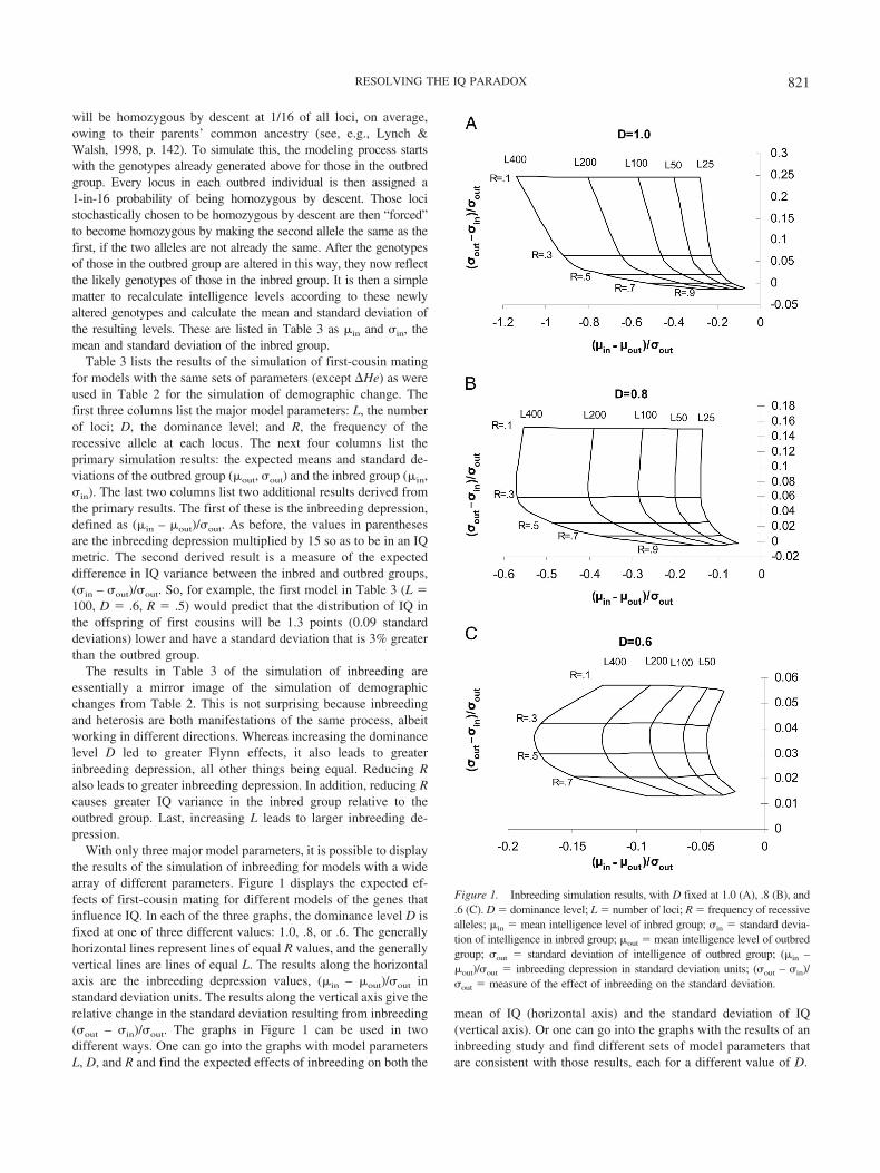
will be homozygous by descent at 1/16 of all loci, on average,owing to their parents’ common ancestry (see, e.g., Lynch &Walsh, 1998, p. 142). To simulate this, the modeling process startswith the genotypes already generated above for those in the outbredgroup. Every locus in each outbred individual is then assigned a1-in-16 probability of being homozygous by descent. Those locistochastically chosen to be homozygous by descent are then “forced”to become homozygous by making the second allele the same as thefirst, if the two alleles are not already the same. After the genotypesof those in the outbred group are altered in this way, they now reflectthe likely genotypes of those in the inbred group. It is then a simplematter to recalculate intelligence levels according to these newlyaltered genotypes and calculate the mean and standard deviation ofthe resulting levels. These are listed in Table 3 as �in and in, themean and standard deviation of the inbred group.

Table 3 lists the results of the simulation of first-cousin matingfor models with the same sets of parameters (except �He) as wereused in Table 2 for the simulation of demographic change. Thefirst three columns list the major model parameters: L, the numberof loci; D, the dominance level; and R, the frequency of therecessive allele at each locus. The next four columns list theprimary simulation results: the expected means and standard de-viations of the outbred group (�out, out) and the inbred group (�in,in). The last two columns list two additional results derived fromthe primary results. The first of these is the inbreeding depression,defined as (�in – �out)/out. As before, the values in parenthesesare the inbreeding depression multiplied by 15 so as to be in an IQmetric. The second derived result is a measure of the expecteddifference in IQ variance between the inbred and outbred groups,(in – out)/out. So, for example, the first model in Table 3 (L �100, D � .6, R � .5) would predict that the distribution of IQ inthe offspring of first cousins will be 1.3 points (0.09 standarddeviations) lower and have a standard deviation that is 3% greaterthan the outbred group.

The results in Table 3 of the simulation of inbreeding areessentially a mirror image of the simulation of demographicchanges from Table 2. This is not surprising because inbreedingand heterosis are both manifestations of the same process, albeitworking in different directions. Whereas increasing the dominancelevel D led to greater Flynn effects, it also leads to greaterinbreeding depression, all other things being equal. Reducing Ralso leads to greater inbreeding depression. In addition, reducing Rcauses greater IQ variance in the inbred group relative to theoutbred group. Last, increasing L leads to larger inbreeding de-pression.

With only three major model parameters, it is possible to displaythe results of the simulation of inbreeding for models with a widearray of different parameters. Figure 1 displays the expected ef-fects of first-cousin mating for different models of the genes thatinfluence IQ. In each of the three graphs, the dominance level D isfixed at one of three different values: 1.0, .8, or .6. The generallyhorizontal lines represent lines of equal R values, and the generallyvertical lines are lines of equal L. The results along the horizontalaxis are the inbreeding depression values, (�in – �out)/out instandard deviation units. The results along the vertical axis give therelative change in the standard deviation resulting from inbreeding(out – in)/out. The graphs in Figure 1 can be used in twodifferent ways. One can go into the graphs with model parametersL, D, and R and find the expected effects of inbreeding on both the

mean of IQ (horizontal axis) and the standard deviation of IQ(vertical axis). Or one can go into the graphs with the results of aninbreeding study and find different sets of model parameters thatare consistent with those results, each for a different value of D.

Figure 1. Inbreeding simulation results, with D fixed at 1.0 (A), .8 (B), and.6 (C). D � dominance level; L � number of loci; R � frequency of recessivealleles; �in � mean intelligence level of inbred group; in � standard devia-tion of intelligence in inbred group; �out � mean intelligence level of outbredgroup; out � standard deviation of intelligence of outbred group; (�in –�out)/out � inbreeding depression in standard deviation units; (out – in)/out � measure of the effect of inbreeding on the standard deviation.


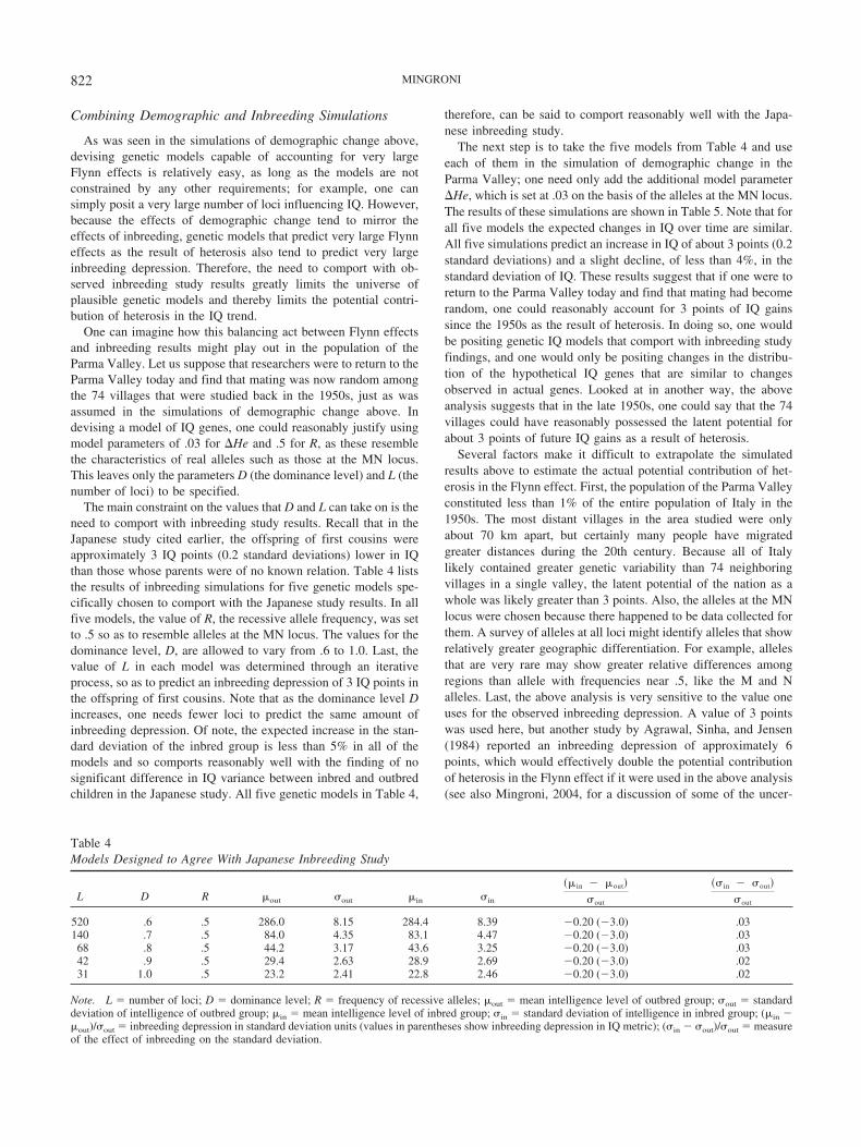
Combining Demographic and Inbreeding Simulations

As was seen in the simulations of demographic change above,devising genetic models capable of accounting for very largeFlynn effects is relatively easy, as long as the models are notconstrained by any other requirements; for example, one cansimply posit a very large number of loci influencing IQ. However,because the effects of demographic change tend to mirror theeffects of inbreeding, genetic models that predict very large Flynneffects as the result of heterosis also tend to predict very largeinbreeding depression. Therefore, the need to comport with ob-served inbreeding study results greatly limits the universe ofplausible genetic models and thereby limits the potential contri-bution of heterosis in the IQ trend.

One can imagine how this balancing act between Flynn effectsand inbreeding results might play out in the population of theParma Valley. Let us suppose that researchers were to return to theParma Valley today and find that mating was now random amongthe 74 villages that were studied back in the 1950s, just as wasassumed in the simulations of demographic change above. Indevising a model of IQ genes, one could reasonably justify usingmodel parameters of .03 for �He and .5 for R, as these resemblethe characteristics of real alleles such as those at the MN locus.This leaves only the parameters D (the dominance level) and L (thenumber of loci) to be specified.

The main constraint on the values that D and L can take on is theneed to comport with inbreeding study results. Recall that in theJapanese study cited earlier, the offspring of first cousins wereapproximately 3 IQ points (0.2 standard deviations) lower in IQthan those whose parents were of no known relation. Table 4 liststhe results of inbreeding simulations for five genetic models spe-cifically chosen to comport with the Japanese study results. In allfive models, the value of R, the recessive allele frequency, was setto .5 so as to resemble alleles at the MN locus. The values for thedominance level, D, are allowed to vary from .6 to 1.0. Last, thevalue of L in each model was determined through an iterativeprocess, so as to predict an inbreeding depression of 3 IQ points inthe offspring of first cousins. Note that as the dominance level Dincreases, one needs fewer loci to predict the same amount ofinbreeding depression. Of note, the expected increase in the stan-dard deviation of the inbred group is less than 5% in all of themodels and so comports reasonably well with the finding of nosignificant difference in IQ variance between inbred and outbredchildren in the Japanese study. All five genetic models in Table 4,

therefore, can be said to comport reasonably well with the Japa-nese inbreeding study.

The next step is to take the five models from Table 4 and useeach of them in the simulation of demographic change in theParma Valley; one need only add the additional model parameter�He, which is set at .03 on the basis of the alleles at the MN locus.The results of these simulations are shown in Table 5. Note that forall five models the expected changes in IQ over time are similar.All five simulations predict an increase in IQ of about 3 points (0.2standard deviations) and a slight decline, of less than 4%, in thestandard deviation of IQ. These results suggest that if one were toreturn to the Parma Valley today and find that mating had becomerandom, one could reasonably account for 3 points of IQ gainssince the 1950s as the result of heterosis. In doing so, one wouldbe positing genetic IQ models that comport with inbreeding studyfindings, and one would only be positing changes in the distribu-tion of the hypothetical IQ genes that are similar to changesobserved in actual genes. Looked at in another way, the aboveanalysis suggests that in the late 1950s, one could say that the 74villages could have reasonably possessed the latent potential forabout 3 points of future IQ gains as a result of heterosis.

Several factors make it difficult to extrapolate the simulatedresults above to estimate the actual potential contribution of het-erosis in the Flynn effect. First, the population of the Parma Valleyconstituted less than 1% of the entire population of Italy in the1950s. The most distant villages in the area studied were onlyabout 70 km apart, but certainly many people have migratedgreater distances during the 20th century. Because all of Italylikely contained greater genetic variability than 74 neighboringvillages in a single valley, the latent potential of the nation as awhole was likely greater than 3 points. Also, the alleles at the MNlocus were chosen because there happened to be data collected forthem. A survey of alleles at all loci might identify alleles that showrelatively greater geographic differentiation. For example, allelesthat are very rare may show greater relative differences amongregions than allele with frequencies near .5, like the M and Nalleles. Last, the above analysis is very sensitive to the value oneuses for the observed inbreeding depression. A value of 3 pointswas used here, but another study by Agrawal, Sinha, and Jensen(1984) reported an inbreeding depression of approximately 6points, which would effectively double the potential contributionof heterosis in the Flynn effect if it were used in the above analysis(see also Mingroni, 2004, for a discussion of some of the uncer-

Table 4Models Designed to Agree With Japanese Inbreeding Study

L D R �out out �in in

��in � �out�

out

�in � out�

out

520 .6 .5 286.0 8.15 284.4 8.39 0.20 (3.0) .03140 .7 .5 84.0 4.35 83.1 4.47 0.20 (3.0) .03

68 .8 .5 44.2 3.17 43.6 3.25 0.20 (3.0) .0342 .9 .5 29.4 2.63 28.9 2.69 0.20 (3.0) .0231 1.0 .5 23.2 2.41 22.8 2.46 0.20 (3.0) .02

Note. L � number of loci; D � dominance level; R � frequency of recessive alleles; �out � mean intelligence level of outbred group; out � standarddeviation of intelligence of outbred group; �in � mean intelligence level of inbred group; in � standard deviation of intelligence in inbred group; (�in �out)/out � inbreeding depression in standard deviation units (values in parentheses show inbreeding depression in IQ metric); (in out)/out � measureof the effect of inbreeding on the standard deviation.

822 MINGRONI

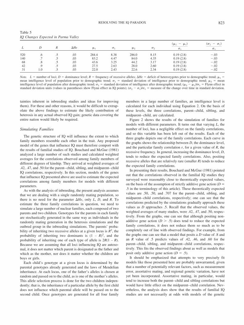
tainties inherent in inbreeding studies and ideas for improvingthem). For these and other reasons, it would be difficult to extrap-olate the above findings to estimate the likely contribution ofheterosis in any actual observed IQ gain; genetic data covering theentire nation would likely be required.

Simulating Families

The genetic structure of IQ will influence the extent to whichfamily members resemble each other in the trait. Any proposedmodel of the genes that influence IQ must therefore comport withthe results of familial studies of IQ. Bouchard and McGue (1981)analyzed a large number of such studies and calculated weightedaverages for the correlations observed among family members ofdifferent degrees of kinship. They arrived at weighted averages of.42, .47, and .50 for the parent–child, sibling, and midparent–childIQ correlations, respectively. In this section, models of the genesthat influence IQ presented above are used to estimate the expectedcorrelations among family members for models with differentparameters.

As with the analysis of inbreeding, the present analysis assumesthat we are dealing with a single randomly mating population, sothere is no need for the parameter �He, only L, D, and R. Toestimate the three family correlations in question, we need tosimulate a large number of nuclear families, each composed of twoparents and two children. Genotypes for the parents in each familyare stochastically generated in the same way as individuals in therandomly mating generation in the heterosis simulations and theoutbred group in the inbreeding simulations. The parents’ proba-bility of inheriting two recessive alleles at a given locus is R2, theprobability of inheriting two dominants is (1 – R)2, and theprobability of inheriting one of each type of allele is 2R(1 – R).Because we are assuming that all loci influencing IQ are autoso-mal, it does not matter which parent is designated as the father andwhich as the mother, nor does it matter whether the children areboys or girls.

Each child’s genotype at a given locus is determined by theparental genotypes already generated and the laws of Mendelianinheritance. At each locus, one of the father’s alleles is chosen atrandom and passed on to the child, as is one of the mother’s alleles.This allele selection process is done for the two children indepen-dently; that is, the inheritance of a particular allele by the first childdoes not influence which parental allele will be passed on to thesecond child. Once genotypes are generated for all four family

members in a large number of families, an intelligence level iscalculated for each individual using Equation 2. On the basis ofthese levels, the three correlations, parent–child, sibling, andmidparent–child, are calculated.

Figure 2 shows the results of the simulation of families formodels with different parameters. It turns out that varying L, thenumber of loci, has a negligible effect on the family correlations,and so this variable has been left out of the results. Each of thethree graphs depicts one of the family correlations. Each curve inthe graphs shows the relationship between D, the dominance level,and the particular family correlation r, for a given value of R, therecessive frequency. In general, increasing the dominance level, D,tends to reduce the expected family correlations. Also, positingrecessive alleles that are relatively rare (smaller R) tends to reducethe expected family correlations.

In presenting their results, Bouchard and McGue (1981) pointedout that the correlations observed in the familial IQ studies theysurveyed were reasonably close to theoretically expected values,on the basis of the assumption of strictly additive gene action (D �.5 in the terminology of this article). These theoretically expectedvalues are .50, .50, and .707 for the parent–child, sibling, andmidparent–child correlations, respectively; one can see that thecorrelations predicted by the simulations gradually approach thesevalues as D approaches .5. Recall that the observed values, theweighted averages of many studies, were .42, .47, and .50, respec-tively. From the graphs, one can see that although positing non-additive gene action (D � .5) does tend to reduce the expectedfamily correlations, it does not reduce them so much as to becompletely out of line with observed findings. For example, fromthe graphs one can see that a model that posits a D value of .8 andan R value of .5 predicts values of .42, .46, and .60 for theparent–child, sibling, and midparent–child correlations, respec-tively. This fits the observed findings about as well as models thatposit only additive gene action (D � .5).

It should be emphasized that attempts to very precisely fitmodels like those presented here are probably unwarranted, giventhat a number of potentially relevant factors, such as measurementerror, assortative mating, and regional genetic variation, have notyet been incorporated. Assortative mating, in particular, wouldtend to increase both the parent–child and sibling correlations butwould have little effect on the midparent–child correlation. Nev-ertheless, the analysis does show that the results of familial IQstudies are not necessarily at odds with models of the genetic

Table 5IQ Changes Expected in Parma Valley

L D R �He �1 1 �2 2

��2 � �1�

1

�2 � 1�

1

520 .6 .5 .03 284.4 8.38 286.0 8.15 0.19 (2.8) .03140 .7 .5 .03 83.2 4.47 84.0 4.35 0.19 (2.8) .03

68 .8 .5 .03 43.6 3.25 44.2 3.17 0.19 (2.8) .0242 .9 .5 .03 27.5 2.63 28.0 2.60 0.19 (2.8) .0231 1.0 .5 .03 22.0 2.43 22.6 2.34 0.19 (2.8) .02

Note. L � number of loci; D � dominance level; R � frequency of recessive alleles; �He � deficit of heterozygotes prior to demographic trend; �1 �mean intelligence level of population prior to demographic trend; 1 � standard deviation of intelligence prior to demographic trend; �2 � meanintelligence level of population after demographic trend; 2 � standard deviation of intelligence after demographic trend; (�2 �1)/1 � Flynn effect instandard deviation units (values in parentheses show Flynn effect in IQ points); (2 1)/1 � measure of the change over time in standard deviation.


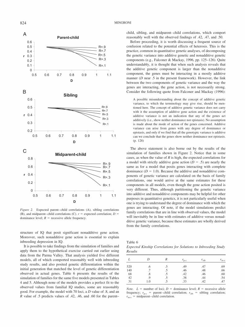
structure of IQ that posit significant nonadditive gene action.Moreover, such nonadditive gene action is essential to explaininbreeding depression in IQ.

It is possible to take findings from the simulation of families andapply them to the hypothetical exercise carried out earlier usingdata from the Parma Valley. That analysis yielded five differentmodels, all of which comported reasonably well with inbreedingstudy results, and also posited genetic differentiation within theinitial generation that matched the level of genetic differentiationobserved in actual genes. Table 6 presents the results of thesimulation of families for the same five models presented in Tables4 and 5. Although none of the models provides a perfect fit to theobserved values from familial IQ studies, some are reasonablygood. For example, the model with 70 loci, a D value of .8, and anR value of .5 predicts values of .42, .46, and .60 for the parent–

child, sibling, and midparent–child correlations, which comportreasonably well with the observed findings of .42, .47, and .50.

Before proceeding, it is worth discussing a frequent source ofconfusion related to the potential effects of heterosis. This is thepractice, common in quantitative genetic analyses, of decomposingthe genetic variance into additive genetic and nonadditive geneticcomponents (e.g., Falconer & Mackay, 1996, pp. 125–126). Quiteunderstandably, it is thought that when such analysis reveals thatthe additive genetic component is larger than the nonadditivecomponent, the genes must be interacting in a mostly additivemanner (D near .5 in the present framework). However, the linkbetween the two components of genetic variance and the way thegenes are interacting, the gene action, is not necessarily strong.Consider the following quote from Falconer and Mackay (1996):

A possible misunderstanding about the concept of additive geneticvariance, to which the terminology may give rise, should be men-tioned here. The concept of additive genetic variance does not carrywith it the assumption of additive gene action and the existence ofadditive variance is not an indication that any of the genes actadditively (i.e., show neither dominance nor epistasis). No assumptionis made about the mode of action of the genes concerned. Additivevariance can arise from genes with any degree of dominance orepistasis, and only if we find that all the genotypic variance is additivecan we conclude that the genes show neither dominance nor epistasis.(p. 128)

The above statement is also borne out by the results of thesimulation of families shown in Figure 2. Notice that in somecases, as when the value of R is high, the expected correlations fora model with strictly additive gene action (D � .5) are nearly thesame as for a model that posits genes interacting with completedominance (D � 1.0). Because the additive and nonadditive com-ponents of genetic variance are calculated on the basis of familycorrelations, one would arrive at the same estimates for thesecomponents in all models, even though the gene action posited isvery different. Thus, although partitioning the genetic varianceinto additive and nonadditive components may be helpful for otherpurposes in quantitative genetics, it is not particularly useful whenone is trying to understand the degree of dominance with which thegenes are interacting. Of note, if the model simulations predictfamily correlations that are in line with observed values, the modelwill inevitably be in line with estimates of additive versus nonad-ditive genetic variance, because these estimates are wholly derivedfrom the family correlations.

Table 6Expected Kinship Correlations for Solutions to Inbreeding StudyResults

L D R rp-c rsib rm-c

520 .6 .5 .49 .47 .69140 .7 .5 .46 .48 .6668 .8 .5 .42 .46 .6042 .9 .5 .38 .44 .5431 1.0 .5 .33 .42 .47

Note. L � number of loci; D � dominance level; R � recessive allelefrequency; rp-c � parent–child correlation; rsib � sibling correlation;rm-c � midparent–child correlation.

Parent-child

R=.1

R=.3

R=.7R=.5

R=.9

0

0.1

0.2

0.30.4

0.5

0.6

0.5 0.6 0.7 0.8 0.9 1 1.1

D

r

Sibling

R=.1

R=.3

R=.5R=.7R=.9

0.2

0.3

0.4

0.5

0.6

0.5 0.6 0.7 0.8 0.9 1 1.1

D

r

Midparent-child

R=.1

R=.3

R=.5R=.7R=.9

0

0.2

0.4

0.6

0.8

0.5 0.6 0.7 0.8 0.9 1 1.1

D

r

A

B

C

Figure 2. Expected parent–child correlations (A), sibling correlations(B), and midparent–child correlations (C). r � expected correlation; D �dominance level; R � recessive allele frequency.

824 MINGRONI

Applicability to Other Trends

Heterosis increases the ratio of heterozygotes to homozygotes atevery polymorphic locus. As such, it is capable of causing simul-taneous trends in multiple polygenic traits. As mentioned earlier,many other heritable traits and conditions have undergone largechanges over time in parallel with the IQ trend. It is possible toadapt the stochastic modeling used above for IQ to try to accountfor these other trends. In the case of some trends, the adaptation isvery simple; in other cases, it is slightly more complicated.

In the case of some traits, such as height, adapting the aboveanalysis merely involves changing the dependent variable in Equa-tion 2 from intelligence to the new trait. Also, because traits likeheight are measured on an absolute scale, the presumed effects onthe trait in Table 1 would not be dimensionless, as they must be inthe case of intelligence, but could be measured in actual units oflength like millimeters. Use of an absolute scale would also placeadditional constraints on the universe of plausible models, becausethe ratio /� would have to comport with empirically observedvalues. There is no way to measure this ratio for intelligence.

Some of the trends do not involve continuously varying traits, inwhich one can observe changes in the entire distribution. Instead,they involve heritable conditions in which the population is di-vided into discrete groups, such as affected versus unaffected. Thetrends in these conditions are measured by changes in the inci-dence of individuals categorized as affected, according to somediagnostic criteria. Conditions like myopia, asthma, and autismbelong to this group. Though still possible, modeling the trends inconditions like these requires making some additional assumptionsabout their underlying genetic structure, as well as some additionalcalculations.

The first step in adapting the above analysis to discontinuoustraits is that one must change the dependent variable in Equation 2from intelligence to something like “liability to myopia” or “ge-netic predisposition to autism.” In this case, one would be assum-ing that all individuals have some genetic liability to the conditionand that this liability is distributed normally in the population.Those affected would represent the upper tail of this presumednormal liability distribution, above some threshold value. Such amodel of the underlying liability to a condition, referred to as apolygenic threshold model, is commonly used in epidemiologicalstudies (Falconer, 1965).

A shift toward more random mating would be capable of caus-ing upward shifts in the presumed liability distributions of discon-tinuous traits in the same way that it is capable of causing shifts inthe distribution of continuously varying traits. As the underlyingliability distribution shifts upward, a larger portion of the popula-tion will fall above the threshold to be considered affected, therebycausing the incidence to rise. For a given change in the incidenceof a condition, it is a simple matter to estimate the magnitude of theshift that would have to take place in its underlying liability inorder to cause the observed rise in incidence. One need only makereference to a table of areas under the normal curve with the earlierand later incidence levels.

As an example, a series of studies in Sweden in the 1980sreported an apparent rise in the incidence of autism, from 4.0/10,000 in 1980 to 11.6/10,000 in 1988 (Gillberg, Steffenburg, &Schaumann, 1991). Such an increase in incidence could be ex-plained by an upward shift in an underlying normal liability to

autism of 0.32 standard deviations in the 8 years (z threshold�3.35 to z threshold �3.03), or about 0.4 standard deviations perdecade. This estimate assumes that there were no changes infactors like diagnostic criteria or ascertainment methods and alsoassumes no change in the variance of the underlying distribution.It should be noted that in the specific case of autism there is stillconsiderable debate among experts as to whether the apparentincreases that have appeared in a number of studies are real, due toartifacts, or both (see, e.g., Gernsbacher, Dawson, & Goldsmith,2005). Obviously, the above analysis would be applicable only ifthe trend were eventually found to be real.

Similarly, an observed increase in asthma from 3.0% to 8.2% in22 years (Upton et al., 2000) could be accounted for by an upwardshift of 0.22 standard deviations per decade. An observed increasein myopia, from 26.3% to 43.3% in approximately 10 years (Stor-fer, 1999), could be accounted for by a shift over time in theunderlying liability to myopia of 0.46 standard deviations perdecade.

It is interesting to note that the rates at which the liabilitydistributions would appear to be shifting are similar to the rates atwhich the distributions of continuous traits like height and IQ haveshifted; these have generally ranged from 0.2 to 0.5 standarddeviations per decade. In the context of a heterosis hypothesis, thiswould suggest that the discontinuous traits have genetic charac-teristics similar to the continuous traits with respect to things likethe number of loci involved, the dominance level, and the ratio ofdominant to recessive genes in the gene pool.

It should be noted that a major problem for the analysis ofdiscontinuous traits is that their incidence will be affected bychanges in both the mean and the variance of the liability distri-butions over time. However, because the trends are measured bychanges in a single variable, the incidence, there is no way todisentangle effects brought about by changes in the mean of thedistribution from effects caused by changes in the variance. Theexamples cited above simply assumed no change in variance;however, future, more detailed modeling efforts would have totake into account the very real possibility that the variance mightbe changing. This will likely mean that the universe of plausiblegenetic structures for the conditions in question may be lessconstrained and therefore less specific.

Growth Saltations

In the case of at least one of the polygenic traits that hasundergone change, height, it may be possible to observe the effectsof individual genes on the phenotype, which opens up a number ofopportunities for testing a heterosis hypothesis. Recent investiga-tions have found that when height is measured frequently, such ason a daily basis, it is possible to discern very fine grained growthspurts, or saltations (Hermanussen et al., 1998; Lampl, 2002). Forexample, a child will sometimes go for a week or two with nodiscernible growth, followed by one or two days in which as muchas a centimeter of growth occurs, followed by another extendedperiod of stasis. Of interest, Lampl (2002, p. 267) cited unpub-lished data suggesting that monozygotic twins resemble one an-other in the pattern of these growth spurts. The similarity ofmonozygotic twins in the timing of saltations raises the possibilitythat each spurt might represent the action of a single gene, or atmost a small number of genes. Such a one-gene/one-saltation


hypothesis generates several testable predictions in the context ofthe present effort to model the genes that influence height.

Within the context of the simple framework outlined in Table 1,a heterosis hypothesis would predict that the trend in height shouldmanifest itself primarily as an increase in the frequency of salta-tions, rather than an increase in the average amplitude of saltations.In fact, unless the genes that influence height interact with com-plete dominance (D � 1.0), the trend in height should actually beaccompanied by a decline over time in the average amplitude ofsaltations, reflecting the increased number of heterozygous lociand the decrease in double dominants. Unfortunately, testing sucha prediction would be difficult, requiring frequent testing of a largenumber of individuals over a long period of time.

A more feasible test might be to compare children in tallpopulations that have already experienced many decades of heightgains with children in shorter, developing countries, whose currentenvironment is comparable to past environments in the now de-veloped populations. In general, a heterosis hypothesis wouldpredict that the difference should be observed mainly as a differ-ence in the frequency, rather than the amplitude, of saltations.Also, it would be interesting to compare inbred children withnoninbred children. Again, a genetic framework like that positedhere would predict that the height difference between the inbredand noninbred groups should appear mainly as a difference in thefrequency of saltations.

The occurrence of identifiable growth saltations also offers thepossibility of testing the plausibility of models of the genes thatinfluence height, such as those presented earlier. According to thesimple framework posited in the present article, if each saltation iscaused by the genes at a single locus, then the number of saltationsthat an average individual experiences up until adulthood shouldbe approximately equal to the average number of loci at whichindividuals inherit either one or two dominant alleles: that is,LDD � LDR. One would probably have to change the assumptionthat all loci have an equal effect on height; hypothesized variationin the effects of different loci would have to match observedvariation in the amplitudes of growth saltations. The simple frame-work presented here would also predict that sex differences inheight should show up as a difference in the amplitude of saltationsrather than in their frequency. Because the present model assumesall loci are autosomal, boys and girls should be affected by thesame number of loci and therefore experience the same overallfrequency of saltations. Thus, one can see that as with otherrelevant empirical findings, the need to comport with growthsaltation studies will likely constrain the universe of plausiblegenetic models.

As mentioned already, the remarkable similarity in height ofmonozygotic twins reared apart, particularly in the earliest studies,conducted in populations that went on to experience large subse-quent increases in height, poses a serious problem for environmen-tal hypotheses for the trend. Such results suggest that any pre-sumed environmental deprivations must have stunted pastpopulations with a remarkable level of uniformity and pervasive-ness, hardly varying at all among households. The study of growthsaltations offers the possibility of measuring this uniformity andpervasiveness in much greater detail. Specifically, if one couldidentify a pair of monozygotic twins currently being reared apart ina developing country, both twins could be measured daily in theirrespective homes. If the twins were to resemble each other in the

timing and amplitude of their growth saltations, it would meaneither that no stunting is occurring in the population or that bothtwins are somehow being stunted by the same amount every week,or even every day, despite living in different homes. Althoughsuch a test would require a unique set of circumstances, it wouldonly entail the measurement of two children for several months. Itmight also be interesting to take pairs of monozygotic twins whoare currently being reared together in a developing country andseparate them for a short while, although ethical considerationswould limit the extent to which one could vary their respectiveenvironmental conditions while measuring them.

Developmental Modeling

In all of the models presented in this article, it has been assumedthat every individual’s phenotype is influenced by the same num-ber of gene loci. This assumption, however, is probably not correctin the case of children. Because different genes will likely havetheir effect on the phenotype at different ages, it would probably bemore appropriate to assume that the phenotype in childhood isinfluenced by fewer genes than the adolescent or adult phenotype.It should be possible to incorporate the likely developmentalnature of genetic influences into the modeling of polygenic traits.

For example, recall that in the simulation of families, alleles ateach locus were randomly passed on from parents to children. Itwould be a simple matter to allow only the alleles at some of theloci to be passed on, so that the phenotypes of the children wouldthen be influenced by only a fraction of the loci that influence theadult phenotype. By gradually increasing the fraction of locipassed on to the children, one could simulate developmentalchanges in the trait in question. One could estimate likely changesin the different family correlations as children get older. One couldalso calculate within-individual correlations at different ages andcompare these with observed findings. In the case of traits likeheight that are measured on an absolute scale, the model wouldalso need to comport with observed developmental changes in boththe mean and standard deviation of the trait.

Incorporating developmental processes into the modeling processwill also influence the interpretation of inbreeding study results aswell as data on time trends, both of which will likely be influenced bythe age of the subjects. Recall that in the models presented above,positing more loci predicts larger inbreeding depression and largerFlynn effects, all other things being equal. In general, then, one wouldinitially expect studies involving younger children to show smallerinbreeding depression and smaller Flynn effects, due to the fact thatthe phenotype in childhood is likely influenced by fewer loci than theadult phenotype. This may provide a partial explanation for theapparent finding of larger Flynn effects in adult samples as comparedto children (Flynn, 1998, p. 27).

Heterosis Hypothesis Predictions

This last section provides a summary of the various testablepredictions of the heterosis hypothesis that have been mentionedthroughout the article. The first four predictions apply to an ob-served trend in any trait or condition, be it a gross physical traitlike height, a behavioral trait like IQ, a threshold trait like asthmaor myopia, or a biochemical trait like the level of a particularhormone. The last prediction deals with traits like height, or

826 MINGRONI

possibly protein levels, in which it may be possible to discern theeffects of individual genes, as manifested by things such as growthspurts or spikes in hormone levels. It must be noted that all of thepredictions below are premised on a strong version of the hypoth-esis in which heterosis is the primary cause of the trend in questionand differences in the genes are the primary cause of variance inthe trait. Obviously, to the extent that other factors may be respon-sible for the trends or contribute substantially to variance, thefollowing expectations may not be fully met.

1. In populations in which the trend in question is occurring, oneshould observe an increase over time in the frequency of heterozy-gotes. More specifically, there should be more families in whichthe parents are more homozygous than their children, on average,at a randomly selected set of gene loci. The reason to lookintergenerationally within families rather than across the entirepopulation is that some segments of the population may be rela-tively more or less homozygous, on average, owing to things likeone segment being descended from a very small founding popu-lation. Differential fertility rates in the different segments couldthen cause a rise or fall in overall heterozygosity rates that wouldobscure what is going on within families.

2. The trait in question should display directional dominance inthe same direction as the trend. Although studies involving indirectmeasures of likely genetic heterozygosity like parental relatednessor parental birthplace may be informative, studies should ideallyexamine the genes of the subjects directly. Specifically, families inwhich there are greater intergenerational increases in heterozygos-ity should account for a greater share of the intergenerationalchanges in the trait. Here again, it is preferable to look withinfamilies because different segments of the population might differin both their average heterozygosity rate and their mean values ofthe trait, creating a spurious correlation between genetic heterozy-gosity and the trait unrelated to the existence of directional dom-inance.

3. It should be possible to develop a model of the genetic structureof the trait whereby observed genetic changes can account for both theobserved phenotypic changes over time and the magnitude of direc-tional dominance observed in the trait. It is important to note that theproposed genetic structure of the trait should not predict outcomes thatconflict with other relevant empirical findings, such as the observedcorrelations among family members or features of the development ofthe trait throughout childhood.

4. The trait in question should not be observed within familiesas one goes from earlier born to later born siblings.

5. In traits like height for which it may be possible to discern theeffects of individual genes, the number of growth saltations should beapproximately equal to the number of loci at which the genes have apositive effect on height in the proposed model of the genetic structureof the trait. Differences in height between tall and short populations,as well as differences between inbred and outbred groups, should becaused primarily by differences in the frequency, rather than theamplitude, of growth saltations. By contrast, sex differences should bethe result of differences in the amplitude of saltations, assuming thatmost of the genes that influence height are autosomal. Also, monozy-gotic twins should resemble one another in both the timing and themagnitude of the saltations, regardless of whether they are living in anaffluent or poor population and whether they are being reared togetheror apart.

Conclusion

For more than two decades now researchers have searched invain for the environmental cause of the Flynn effect, and it seemsunlikely that such a cause will be identified soon. The reason forsuch pessimism is that the IQ paradox renders all environmentalhypotheses implausible, untestable, or both. For example, one canlook to identifiable factors like nutrition and education, but giventhe high heritability of IQ, the associations between cause andeffect will not persist beyond the ecological level. Any postnatalfactor, even one with the characteristics of a factor X, is problem-atic because it must have either a shared-family component, anonshared component, or both. However, MZA twin and adoptionstudies suggest the cause does not have a large shared component,and birth order studies suggest it does not have a large nonsharedcomponent. The only environmental factors with much hope ofresolving the paradox are shared prenatal factors, or environmentalfactors that are so highly correlated with the genes as to beindistinguishable from them. Even these face the problem of thestability of IQ heritability over time. Moreover, even if factors ofthis type are responsible for the Flynn effect, their very naturemakes it difficult to disentangle their effects from those of geneticfactors, making them inherently difficult to identify or measure.

If, however, the Flynn effect is genetic in origin, the IQ paradox isnot only resolved, it is eliminated; there is nothing paradoxical toexplain. And the only plausible genetic cause yet proposed is hetero-sis. Perhaps most important, and in contrast to most environmentalhypotheses, a heterosis hypothesis generates numerous predictionsthat can be tested empirically. In a world of limited resources, scien-tists rarely have the option of pursuing in great depth every hypothesisput forward to explain a particular phenomenon. Instead, it is usuallynecessary to engage in a kind of cost–benefit analysis, focusingmainly on those lines of inquiry that seem most likely to advance ourunderstanding of the phenomena in question. In light of its plausibil-ity, testability, and potential to explain multiple phenomena, a hetero-sis hypothesis for the Flynn effect represents a working hypothesissuperior to any yet proposed. It is important to point out that even ifthe hypothesis is eventually disproved, the process of testing it islikely to provide clues to the eventual cause, whatever that may be, aswell as clues to the genetic structure of the traits and conditions inquestion. Considering that there is so much to be gained and so littleto lose, the testing of a heterosis hypothesis should be the primaryfocus of future efforts to better understand the cause of the worldwiderise in IQ test scores.

References

Agrawal, N., Sinha, S. N., & Jensen, A. R. (1984). Effects of inbreeding onRaven matrices. Behavior Genetics, 14, 579–585.

Alroy, J. (1998, May 1). Cope’s rule and the dynamics of body massevolution in North American fossil mammals. Science, 280, 731–734.

Anderson, A. M. (1982, May 20). The great Japanese IQ increase. Nature,297, 181–182.

Barber, N. (2005). Educational and ecological correlates of IQ: A cross-national investigation. Intelligence, 33, 273–284.

Belmont, L., & Marolla, F. A. (1973, December 14). Birth order, familysize, and intelligence. Science, 182, 1096–1101.

Billy, G. (1980). Microevolution and exogamy. In I. Schwidetzky, B.Chiarelli, & O. Necrasov (Eds.), Physical anthropology of Europeanpopulations (pp. 59–68). The Hague, the Netherlands: Mouton.


Bouchard, T. J., Jr., Lykken, D. T., McGue, M., Segal, N. L., & Tellegen,A. (1990, October 12). Sources of human psychological differences: TheMinnesota Study of Twins Reared Apart. Science, 250, 223–228.

Bouchard, T. J., Jr., & McGue, M. (1981, May 29). Familial studies ofintelligence: A review. Science, 212, 1055–1059.

Brand, C. (1987, August 27). Keeping up with the times. Nature, 328, 761.Brinkman, H. J., Drukker, J. W., & Slot, B. (1988). Height and income: A

new method for the estimation of historical national income series.Explorations in Economic History, 25, 227–264.

Capron, C., & Duyme, M. (1996). Effect of socioeconomic status ofbiological and adoptive parents on WISC–R subtest scores of theirFrench adopted children. Intelligence, 22, 259–275.

Carroll, J. B. (1993). Human cognitive abilities: A survey of factor-analyticstudies. New York: Cambridge University Press.

Cavalli-Sforza, L. L., Moroni, A., & Zei, G. (2004). Consanguinity, inbreed-ing, and genetic drift in Italy. Princeton, NJ: Princeton University Press.

Colom, R., Lluis-Font, J. M., & Andres-Pueyo, A. (2005). The generationalintelligence gains are caused by decreasing variance in the lower half ofthe distribution: Supporting evidence for the nutrition hypothesis. Intel-ligence, 33, 83–91.

Comings, D. E. (1996). The gene bomb. Duarte, CA: Hope Press.Cook, E. H., Jr., & Leventhal, B. L. (1996). The serotonin system in

autism. Current Opinion in Pediatrics, 8, 348–354.Dahlberg, G. (1942). Race, reason and rubbish. London: Allen & Unwin.Damon, A. (1965). Stature increase among Italian-Americans: Environ-

mental, genetic, or both? American Journal of Physical Anthropology,23, 401–408.

Deary, I. J. (2001). Intelligence: A very short introduction. Oxford, En-gland: Oxford University Press.

Dickens, W. T., & Flynn, J. R. (2001). Heritability estimates versus largeenvironmental effects: The IQ paradox resolved. Psychological Review,108, 346–369.

Dickens, W. T., & Flynn, J. R. (2002). The IQ paradox is still resolved:Reply to Loehlin (2002) and Rowe and Rodgers (2002). PsychologicalReview, 109, 764–771.

Drukker, J., & Van Meerten, M. (1995). Beyond Villerme and Quetelet:The quantitative relation between sex- and age-specific height and realper capita income. In J. Komlos (Ed.), The biological standard of livingon three continents: Further explorations in anthropometric history (pp.25–58). Boulder, CO: Westview Press.

Ernst, C., & Angst, J. (1983). Birth order: Its influence on personality.Berlin, Germany: Springer-Verlag.

Falconer, D. S. (1965). The inheritance of liability to certain diseases,estimated from the incidence among relatives. Annals of Human Genet-ics, 29, 51–76.

Falconer, D. S., & Mackay, T. F. C. (1996). Introduction to quantitativegenetics (4th ed.). Essex, England: Longman.

Ferak, V., Lichardnova, Z., & Borjinova, V. (1968). Endogamy, exogamyand stature. Eugenics Quarterly, 15, 273–276.

Fisher, R. A. (1928). The possible modification of the wild type torecurrent mutations. American Naturalist, 62, 115–126.

Fisher, R. A. (1931). The evolution of dominance. Biological Reviews, 6,345–368.

Flynn, J. R. (1987). Massive IQ gains in 14 nations: What IQ tests reallymeasure. Psychological Bulletin, 101, 171–191.

Flynn, J. R. (1994). IQ gains over time. In R. J. Sternberg (Ed.), Encyclo-pedia of human intelligence (pp. 617–623). New York: Macmillan.

Flynn, J. R. (1998). IQ gains over time: Toward finding the causes. In U.Neisser (Ed.), The rising curve: Long-term gains in IQ and relatedmeasures (pp. 25–66). Washington, DC: American Psychological As-sociation.

Gernsbacher, M. A., Dawson, M., & Goldsmith, H. H. (2005). Threereasons not to believe in the autism epidemic. Current Directions inPsychological Science, 14, 55–58.

Gillberg, C., Steffenburg, S., & Schaumann, H. (1991). Is autism morecommon now than ten years ago? British Journal of Psychiatry, 158,403–409.

Gottfredson, L. S. (1997). Why g matters. Intelligence, 24, 13–23.Gould, S. J., & Eldredge, N. (1977). Punctuated equilibria: The tempo and

mode of evolution reconsidered. Paleobiology, 3, 115–151.Hanson, R., Smith, J. A., & Hume, W. (1985). Achievements of infants on

items of the Griffiths scales: 1980 compared to 1950. Child Care,Health, and Development, 11, 91–104.

Helgason, A., Yngvadottir, B., Hrafnkelsson, B., Gulcher, J., & Stefansson,K. (2005). An Icelandic example of the impact of population structure onassociation studies. Nature Genetics, 37, 90–95.

Hermanussen, M., Thiel, C., von Buren, E., De Los Angeles, M., De Lama,R., Perez Romero, A., et al. (1998). Micro and macro perspectives inauxology: Findings and considerations upon the variability of short termand individual growth and the stability of population derived parameters.Annals of Human Biology, 25, 359–385.

Hulse, F. (1964). Exogamy and heterosis. In G. W. Lasker (Ed.), Yearbookof physical anthropology (pp. 241–257). Washington DC: AmericanAssociation of Physical Anthropologists.

Hunter, J. E., & Hunter, R. F. (1984). Validity and utility of alternativepredictors of job performance. Psychological Bulletin, 96, 72–98.

Jensen, A. R. (1983). Effects of inbreeding on mental-ability factors.Personality and Individual Differences, 4, 71–87.

Jensen, A. R. (1998). The g factor: The science of mental ability. Westport,CT: Praeger.

Jensen, A. R., & Sinha, S. N. (1993). Physical correlates of humanintelligence. In P. A. Vernon (Ed.), Biological approaches to the studyof human intelligence (pp. 139–242). Norwood, NJ: Ablex.

Kacser, H., & Burns, J. A. (1981). The molecular basis of dominance.Genetics, 97, 639–666.

Kane, H., & Oakland, T. D. (2000). Secular declines in Spearman’s g:Some evidence from the United States. Journal of Genetic Psychology,161, 337–345.

Kehle, T. J., Bray, M. A., Theodore, L. A., Zhou, Z., & McCoach, D. B.(2004). Emotional disturbance/social maladjustment: Why is the inci-dence increasing? Psychology in the Schools, 41, 861–865.

Kimura, M. (1983). The neutral theory of molecular evolution. Cambridge,England: Cambridge University Press.

Komlos, J. (Ed.). (1994). Stature, living standards, and economic development:Essays in anthropometric history. Chicago: University of Chicago Press.

Komlos, J. (Ed.). (1995). The biological standard of living on threecontinents: Further explorations in anthropometric history. Boulder,CO: Westview Press.

Lampl, M. (2002). Saltation and stasis. In N. Cameron (Ed.), Humangrowth and development (pp. 253–270). Amsterdam, the Netherlands:Academic Press.

Loehlin, J. C. (2002). The IQ paradox: Resolved? Still an open question.Psychological Review, 109, 754–758.

Loehlin, J. C., Horn, J. M., & Willerman, L. (1989). Modeling IQ change:Evidence from the Texas Adoption Project. Child Development, 60,993–1004.

Lubke, G. H., Dolan, C. V., Kelderman, H., & Mellenbergh, G. J. (2003).On the relationship between sources of within- and between-groupdifferences and measurement invariance in the common factor model.Intelligence, 31, 543–566.

Lynch, M., & Walsh, B. (1998). Genetics and analysis of quantitativetraits. Sunderland, MA: Sinauer.

Lynn, R. (1998a). The decline of genotypic intelligence. In U. Neisser(Ed.), The rising curve: Long-term gains in IQ and related measures (pp.335–364). Washington, DC: American Psychological Association.

Lynn, R. (1998b). In support of the nutrition theory. In U. Neisser (Ed.),The rising curve: Long-term gains in IQ and related measures (pp.207–218). Washington, DC: American Psychological Association.

828 MINGRONI

Mingroni, M. A. (2004). The secular rise in IQ: Giving heterosis a closerlook. Intelligence, 32, 65–83.

Mueller, W. H. (1986). The genetics of size and shape in children andadults. In F. Falkner & J. M. Tanner (Eds.), Human growth: A compre-hensive treatise (Vol. 3, pp. 145–168). New York: Plenum Press.

Murray, C. (1997). IQ and economic success. Public Interest, 128, 21–35.Neisser, U. (1998). The rising curve: Long-term gains in IQ and related

measures. Washington, DC: American Psychological Association.Neisser, U., Boodoo, G., Bouchard, T. J., Jr., Boykin, A. W., Brody, N.,

Ceci, S. J., et al. (1996). Intelligence: Knowns and unknowns. AmericanPsychologist, 51, 77–101.

Newman, H. H., Freeman, F. N., Holzinger, K. J. (1937). Twins: A studyof heredity and environment. Chicago: University of Chicago Press.

Pedersen, N. L., Plomin, R., Nesselroade, J. R., & McClearn, G. E. (1992).A quantitative genetic analysis of cognitive abilities during the secondhalf of the life span. Psychological Science, 3, 346–353.

Plomin, R., Fulker, D. W., Corley, R., & DeFries, J. C. (1997). Nature,nurture, and cognitive development from 1 to 16 years: A parent–offspring adoption study. Psychological Science, 8, 442–447.

Raven, J., Raven, J. C., & Court, J. H. (1998). Manual for Raven’sProgressive Matrices and Vocabulary Scales: Section 1. General Over-view. Oxford, England: Oxford Psychologists Press, and San Antonio,TX: Psychological Corporation.

Rodgers, J. L. (1999). A critique of the Flynn effect: Massive IQ gains,methodological artifacts, or both? Intelligence, 26, 337–356.

Rodgers, J. L., Cleveland, H. H., van den Oord, E., & Rowe, D. C. (2000).Resolving the debate over birth order, family size and intelligence.American Psychologist, 55, 599–612.

Rowe, D. C., Jacobson, K. C., & Van den Oord, J. C. G. (1999). Geneticand environmental influences on vocabulary IQ: Parental education levelas moderator. Child Development, 70, 1151–1162.

Rowe, D. C., & Rodgers, J. L. (2002). Expanding variance and the case ofhistorical changes in IQ means: A critique of Dickens and Flynn.Psychological Review, 109, 759–763.

Rutter, M., & Silberg, J. (2002). Gene environment interplay in relation toemotional and behavioral disturbance. Annual Review of Psychology, 53,463–490.

Rutter, M., & Smith, D. J. (Eds.). (1995). Psychosocial disorders in youngpeople: Time trends and their causes. Chichester, England: Wiley.

Scarr, S., & Weinberg, R. A. (1978). The influence of “family background”in intellectual attainment. American Sociological Review, 43, 674–692.

Schreider, E. (1969). Inbreeding, biological and mental variations inFrance. American Journal of Physical Anthropology, 30, 215–220.

Schull, W. J., & Neel, J. V. (1965). The effects of inbreeding on Japanesechildren. New York: Harper & Row.

Shapiro, H. L. (1936). The heritage of the Bounty: The story of Pitcairnthrough six generations. New York: Simon & Schuster.

Shih, Y. F., Hsiao, C. K., Chen, C. J., Chang, C. W., Hung, P. T., & Lin,L. L. K. (2001). An intervention trial on the efficacy of atropine andmulti-focal glasses in controlling myopic progression. Acta Ophthalmo-logica Scandinavica, 79, 233–236.

Sibbald, B. (1997). Familial inheritance of asthma and allergy. In A. B.Kay (Ed.), Allergy and allergic diseases (Vol. 2, pp. 1177–1186).London: Blackwell Science.

Steckel, R., & Floud, R. (Eds.). (1997). Health and welfare during indus-trialization. Chicago: University of Chicago Press.

Stein, Z., Susser, M., Saenger, G., & Marolla, F. (1972, November 17).Nutrition and mental performance. Science, 178, 708–713.

Stoolmiller, M. (1999). Implications of the restricted range of family environ-ments for estimates of heritability and nonshared environment in behavior-genetic adoption studies. Psychological Bulletin, 125, 392–409.

Storfer, M. (1999). Myopia, intelligence, and the expanding human neo-cortex: Behavioral influences and evolutionary implications. Interna-tional Journal of Neuroscience, 98, 153–276.

Sundet, J. M., Barlag, D. G., & Torjussen, T. M. (2004). The end of the Flynneffect? A study of secular trends in mean intelligence test scores of Nor-wegian conscripts during half a century. Intelligence, 32, 349–362.

Tanner, J. M. (1981). A history of the study of human growth. Cambridge,England: Cambridge University Press.

Tanner, J. M. (1990). Foetus into man: Physical growth from conception tomaturity. Cambridge, MA: Harvard University Press.

Tanner, J. M. (1994). Introduction: Growth in height as a mirror of thestandard of living. In J. Komlos (Ed.), Stature, living standards, andeconomic development: Essays in anthropometric history (pp. 1–6).Chicago: University of Chicago Press.

Tasbihsazan, R., Nettelbeck, T., & Kirby, N. (1997). Increasing mental devel-opment index in Australian children: A comparative study of two versionsof the Bayley Mental Scale. Australian Psychologist, 32, 120–125.

Teasdale, T. W., & Owen, R. (2000). Forty-year secular trends in cognitiveabilities. Intelligence, 28, 115–120.

Teasdale, T. W., & Owen, R. (2005). A long-term rise and recent declinein intelligence test performance: The Flynn effect in reverse. Personalityand Individual Differences, 39, 837–843.

Upton, M. N., McConnachie, A., McSharry, C., Hart, C. L., Smith, G. D.,Gillis, C. R., & Watt, G. C. M. (2000). International 20 year trends in theprevalence of asthma and hay fever in adults: The Midspan family studysurveys of parents and offspring. British Medical Journal, 321, 88–92.

Van Wieringen, J. C. (1986). Secular growth changes. In F. Falkner &J. M. Tanner (Eds.), Human growth: A comprehensive treatise (Vol. 3,pp. 307–331). New York: Plenum Press.

Wechsler, D. (1991). The Wechsler Intelligence Scale for Children—ThirdEdition. San Antonio, TX: Psychological Corporation.

Wicherts, J. M., Dolan, C. V., Hessen, D. J., Oosterveld, P., van Baal,G. C. M., Boomsma, D. I., & Span, M. S. (2004). Are intelligence testsmeasurement invariant over time? Investigating the nature of Flynneffect. Intelligence, 32, 509–537.

Williams, W. (1998). Are we raising smarter children today? School- andhome-related influences on IQ. In U. Neisser (Ed.), The rising curve:Long-term gains in IQ and related measures (pp. 125–154). Washing-ton, DC: American Psychological Association.

Wilson, R. S. (1986). Growth and development of human twins. In F.Falkner & J. M. Tanner (Eds.), Human growth: A comprehensive trea-tise (Vol. 3, pp. 197–211). New York: Plenum Press.

Wolanski, N., Jarosz, E., & Pyzuk, M. (1970). Heterosis in man: Growthin offspring and distance between parents’ birthplaces. Social Biology,17, 1–16.

Wright, S. (1934). Molecular and evolutionary theories of dominance.American Naturalist, 63, 24–53.

Zajonc, R. B., & Mullally, P. R. (1997). Birth order: Reconciling conflict-ing effects. American Psychologist, 52, 685–699.

Received February 24, 2006Revision received November 1, 2006

Accepted January 3, 2007 �


Correction to Mingroni (2007)

In the article “Resolving the IQ Paradox: Heterosis as a Cause of the Flynn Effect and OtherTrends,” by Michael A. Mingroni (Psychological Review, 2007, Vol. 114, No. 3, pp. 806–829), anequation appearing on page 821 in the text and in Figure 1 was incorrect. The equation (out in)/out appearing on the third line from the bottom of the left column of text; as the y-axis labelsin Figure 1, Panels A, B, and C; and in the next-to-last and last lines of the caption to Figure 1 shouldbe (in out)/out in all these places.

resolving the iq paradox: heterosis as a cause of the ... · resolving the iq paradox: heterosis as...

Documents