RESONANT WHIRLING OF TWO-PIECE PROPSHAFTS INREAR- WHEEL-DRIVE CARS

1. Introduction

Many modern cars with rear-wheel drives have a two-piece, rather than thetraditional one-piece, props haft (or tail-shaft). The cars include Holden Com-modores, Nissans and many European makes. The two-piece shaft requires lessfloor clearance, and hence a smaller floor tunnel, and does not suffer from thehigh-speed twisting resonances to which the one-piece shaft is susceptible.

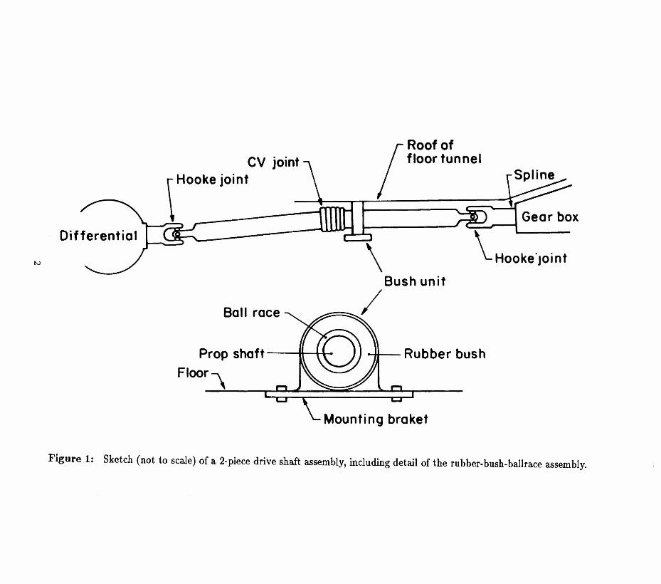
The two-piece shaft is, however, susceptible to a lower speed, high load (hightorque) phenomenon in which the propshaft whirls with increasing amplitudeuntil its restraining rubber bush is fully compressed in its mounting bracket(see Figure 1), causing a thump sound. The whirling amplitude builds upperiodically, so that a regular series of thumps is heard at a frequency of about5 per second.

The effect is very sensitive to the properties of the rubber bush and to itstemperature. Different designs of bush are used by different makers, each withthe purpose of minimizing both the whirling problem and the transmission ofother vibrations to the car body. GMH has a particular design which it wouldprefer not to vary, because of retooling costs. It can however vary the propertiesof the rubber material itself. By trial and error it has achieved rubber prop-erties which control the whirling problem to an acceptable level under normalconditions. GMH posed the question, to the MISG, of whether one can givetheoretical guidelines for optimal rubber properties. This might leadto improved control of the whirling problem. It would also be useful for newand modified propshafts, if it could replace the tedious trial and error processpreviously employed.

GMH were also anxious to gain a better understanding of the whirling phe-nomenon, and felt, with us, that a mathematical description of the phenomenonwas a prerequisite for the study of the rubber properties.

The thumping phenomenon is observed at both 40 and 80 kph approximately,although the phenomenon had a different quality at these two speeds. The2:1 ratio between these speeds suggests that a fundamental resonance and aharmonic resonance are responsible. Such multiple resonances are typical ofnon-linear oscillating systems, so we looked for non-linear driving forces.

The tail-shaft has a natural frequency of oscillation, in its rubber bush, ofabout 40cps. A prime candidate for exciting this oscillation was the Hooke joints

1

IRoof offloor tunnel

Prop shaft -----'1tt--t-\-

Floor"-L-,~~~~~ __

\Bush unit

~/\ HooksjointN

-u-- Rubber bush

Figure 1: Sketch (not to scale) of a 2-piece drive shaft assembly, including detail of the rubber-bush-ballrace assembly.

•••r ~----~--------·~cv~~

et>

Figure 2: Schematic illustration of the simplified model showing various constants and variables.

r

(see Figure 1). These are known to impose oscillatory torques on the shafts theyconnect. The torques are known to excite torsional elastic oscillations in one-piece tail-shafts at higher speeds and frequencies (Zahradka 1973).

A miniature model of the tail-shaft assembly was built using Technic Lego,in a configuration resembling Figure 1. Hooke universal joints were used forall joints, rubber bands were used to approximate the rubber bush and theshaft was driven by an electric motor. The shaft-cum-rubber-band system hada natural frequency of about 20cps. It was found possible to excite resonanceat this frequency by tuning the speed of the motor precisely. When the shaftswere all in a straight line, no such resonance was found. This rather primitiveexperiment showed that Hookejoints between angled shafts could be the drivingforce in the real system, and so the dynamics of this effect was studied. Otherpossible driving forces were discussed and eliminated to the group's satisfaction.

2. The dynamics of a simplified model

Figure 2 illustrates the simplified model that was analysed. The mass of thetail-shaft was replaced by a single point mass m coincident with the constantvelocity (CV) joint. Real tail-shafts have moments of inertia and exhibit gy-roscopic effects. There is no great difficulty in including such effects, but ourprimary aim was to focus on the crux of the resonance phenomena. Inclusion ofall sorts of additional but inessential effects seemed likely to cloud the issue.

The rubber bush was taken as coincident with m. The front half of the shaftis nearly parallel to the gearbox shaft so that the front Hooke joint behaves likea CV joint. The real angle at this joint was given as no more than 10, while theother joints were at varying angles of around 40, so this approximation seemedsatisfactory. However, for simplicity, we adopted the geometry shown in Figure2, while retaining the front CV joint.

The angles (J, </>,.,p in Figure 2 are the Euler angles of rod Om relative to a:fixedframe through O. The angle (J was taken as fixed because it was known thatthe spline joint tended to freeze up under load, preventing significant change in(J. A flywheel of moment of inertia C was located as shown. This was intendedto represent the inertia of all the rotating car components connected to thetail-shaft itself. So C would include the rotating parts of the engine, gear box,differential, axles and the wheels (and, indirectly, the linear inertia of the carplus load, though decoupled somewhat by the rubber tyres).

Equal and opposite torques r are applied at the two ends of the system. Nodamping forces are included, because these seemed inessential to an understand-ing of the phenomenon.

4

The system has only 2 degrees of freedom, described by the 2 generalized co-ordinates t/> and 'I/J. Evidently the system (with I''s included) is a self-containedconservative system. Energy can be exchanged between the mass m, the fly-wheel, the torques and the rubber bush. The whirling phenomenon would cor-respond to oscillations in t/>.

A Lagrangian formulation of the dynamics is convenient because it dealseasily with generalized coordinates and because it does not involve the rathercomplex forces and torques at the Hookejoints. Only the forces that do work (theT''s and the rubber bush forces) need be considered. The Lagrangian equationstake the form (dots denote time derivatives).

d (aT) er =dt 7iJ; - a<l>

d (aT) er =dt a~ - a'I/J

av- at/>

av- a'I/J (1)

where T is the kinetic energy and V is the potential energy of the system. Theflywheel has angular velocity ~ + 4> shown in Figure 2. The mass m has linearvelocity 4>£sinfJ with £ being the distance from 0 to m as shown in Figure 2.Thus

1· 2 1 . . 2T = 2"m( t/>£sin fJ) + 2"C( 'I/J + <1» (2)

We suppose, for simplicity, that the rubber bush is ideally elastic and exerts aforce ks where k is a stiffness constant and s = <I>£sinfJ is the displacement of malong its circular path. The potential energy due to the torques I' is the negativeof the work done by the torques. Noting the angles in Figure 2 we thus have

V = ~k( <1>£sin fJ) + I'( 'I/J + t/> - (3)

A standard relation for Hooke joints is (Wagner and Cooney 1979).

f3.A. • [ sin'I/J 1= 'f' + arcsm 1(1 - sin2 fJ cos2 'I/J) 2'

(3)

(4)

For equations (1) we need

af3 cos fJa'I/J = 1 - sin2 fJ cos2 'I/J (5)

Substituting (2), (3) and (5) in (1) gives

(m£2 sin2 fJ)4> + C(;fi + 4» = -( k£2 sin2 fJ)t/>

C( ~ +~) = [cosfJ/(1 - sin2 fJ cos2 'I/J) - l]f (6)

5

We take initial conditions

,p(0) = 0, ~(O) = 0

with various <p(0) and ,j,(0). Since (J is of order 4°, we can expand the sines andcosines and keep only terms up to (J2. Then equations (6) combine to give

w-2~ = -<p+Acos(2,p)w-2~ = <p- B cos(2,p)

(7)

where w = (klm)t is the natural frequency of the system,

A = r1(2kl2),

B = A(l + m£2(J2IG) (8)

A convenient simplification is to put T = wt. Then

<p" =,p"

-<p - Acos(2,p)<p+ B cos(2,p) (9)

where (') = (dldT).

The dimensionless constants A and B summarize the physical regime inwhich we are interested. For VN Commodores

k ~ l06Nlmr ~ 290Nm£ ~ Im

whenceA ~ 1.5 X 10-4

We note that B IA measures the ratio of the moment of inertia of flywheelplus m to flywheel alone. Since G represents many inertial parts, we expectG» ml2(J2, whence

Then (9) gives<p"+ ,p" = 0

so that

where N = ,j,(O)lw and T = T + <p(O)IN. Using ~ for <pwe now have

~"= -~ + Acos(2NT - 2~). (10)

6

This is the equation upon which our subsequent discussion is based. We see thatit resembles a simple harmonic oscillation (SRO) with a forcing term of smallamplitude A. Prior to resonance we would expect ~ to be small, so that

~"~ -~ + Acos(2NT). (11)

This linear equation exhibits resonance at N = t, so we would expect reso-nance in (10) at this N. The non-linear ~ dependence in (10), however, gives aresonance which grows and develops in a fashion radically different from (11).

3. The resonant behaviour

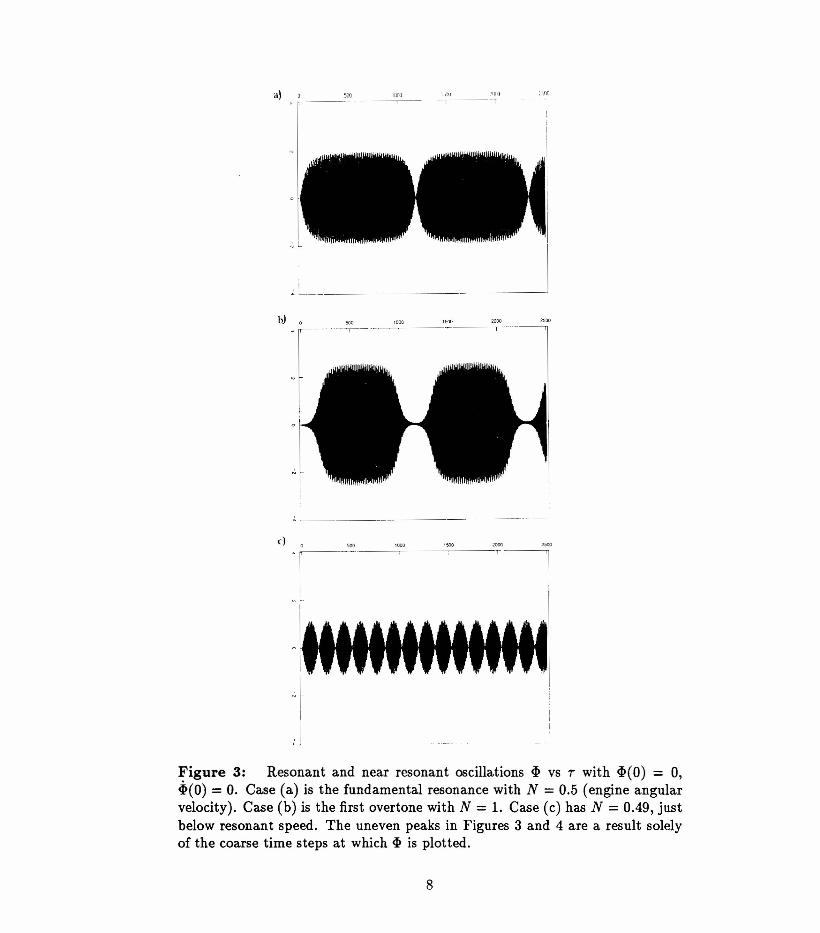
Figure 3 gives a suite of solutions of (10) for a several values of Nand~(O) = 0 obtained by numerical computation using IMSL routine IVPRK. Wetook A = 0.05, larger than its true value, so that individual oscillations areclearer. We noted the expected resonance at N = ! (figure 3a) plus othersat N = t and N = 1 (Figure 3b). The resonances do not persist, but ratherthey grow and die away in periodic fashion. As N moves away from a resonantvalue, the period of this envelope decreases quite rapidly as does the amplitude(Figure 3c).

This periodic surging in the resonant behaviour seems quite close to GMR'sdescription of the thumping phenomenon. The peak amplitudes are potentialthumps, since the peaks occur at a frequency much less than N. We cannot makea more quantitative comparison at this stage because of the simplifications inour model.

The resonances can be derived theoretically as follows. In (10) weput Y = 2~,TI = 2N and 0 = 2A, which gives

y" + Y = 0 cos(y - TIT). (12)

For 0 « 1 and T « 1/0 we can obtain a solution Y(T) in powers of 0 via therecursion

Yo

"Yj+1 + Yj+1

oo cos(Yj - TIT) (13)

for j = 0,1,2, ... , with Yj(O) = Yj(O) = O. Thus

yr + Yl = 0 cos(TIT)

with solutiono

Yl = -1--2[cos(TIT) - cosT]-TI

(14)

7

lOon 1'~l\) ;'I]l1.1~r----T

!II

..~

bl 0 5<)0

. f~----'----I

1000 1500 2000 2500--- ----T --- --------0]

cl 0 >00

. "-----1' -----------'-----'--------T I,

ascc

~IIi

, !

Figure 3: Resonant and near resonant oscillations (1) vs T with (1)(0) = 0,~(O) = O. Case (a) is the fundamental resonance with N = 0.5 (engine angularvelocity). Case (b) is the first overtone with N = 1. Case (c) has N = 0.49, justbelow resonant speed. The uneven peaks in Figures 3 and 4 are a result solelyof the coarse time steps at which <l) is plotted.

8

This shows the expected fundamental resonance at 7] = l(N = !). The nextiterate satisfies

The 0(02) driving terms imply that Y2 has resonances at

7] + 1 = 1, 27] = 1 and 7] - 1 = 1

Le. 7] = O,! and 2 (N = 0, t and 1). The values N = t and 1 are the first under-tone and first overtone of the fundamental resonance N = ~. The coefficient02

indicates a more slowly growing resonance compared to the fundamental. Thisis consistent with Figure 3b. The N = 0 resonance is an artifact of the simplifi-cation leading to (10), which effectivelygives the external system infinite inertia(C = 00). Thus the system can have a spurious energy even when N = O.

Since these solutions are valid only for small T, they predict only the onsetof resonance, not its later development.

It seems likely that the fundamental (N = !) and first overtone (N = 1)resonances correspond to the observed thumping phenomena at 40kph and 80kph.

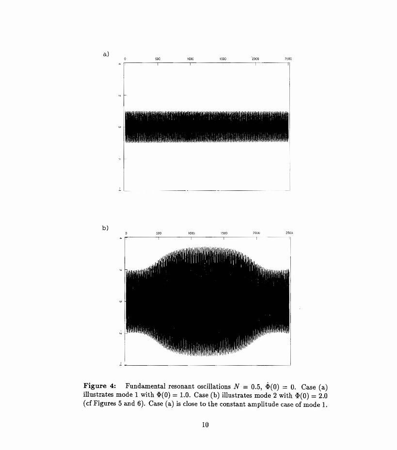
For CIi(O) i- 0 one finds other modes of oscillation. We illustrate in Figure4 how the fundamental resonance, N = !, varies as CIi(O) increases. We shallclassify these modes further in Section 4.

4. Asymptotic analysis

The technique developed by Krylov and Bogoliubov (see Bogoliubov andMetropolski 1961 (BM)) enables one to find the amplitude (and phase) of theenvelopes of the solution curves, like those shown in Figures 3 and 4. First wewrite our equation in the notation of BM:

(17)with

J(T, z , i:) = cos(T - x), (18)where e = 2w2 A, x = 2CIi and v = 2.J,(0). BM represent solutions of(17) in theform

x(t) = aCt) cos[vt + Set)] + O(g) (19)

9

a)500 1000 1500 2500

,1 [ I I I • '~I t" f I '

I' !, .' 'j {,' 1 T ' • Itl} I

,

"

J_. __

b)500 1000 1500 2000 2500

,"

~~--------------------------------------~

Figure 4: Fundamental resonant oscillations N = 0.5, 4>(0) = O. Case (a)illustrates mode 1 with ~(O) = 1.0. Case (b) illustrates mode 2 with ~(O) = 2.0(cf Figures 5 and 6). Case (a) is close to the constant amplitude case of mode 1.

10

Typically one finds that aCt) and e(t) vary slowly compared to cos(vt), so theydescribe the envelope of the fast oscillations. BM, (14.4), obtain an asymptoticexpansion for a and e in powers of e. To first order these are given by (BM(14.25) with p = q = 1)

dedt

(20)

(21)

where

Gu(a)

and (BM (14.4))

(22)

(23)

lo(a,O, t/J) - 1(0, a cos t/J, - ~avsin t/J)

= cos(0 - a cos t/J) (24)

Note that the integration variables 0 and t/J bear no relation to our originalEuler angles.

We evaluate the integrals in stages. First, for Fu, we need

2.. t=dOe-iu(1/J-9)cos(O-acost/J) = eiu(acos1/J-1/J)2.. i" d,peiut/>cos,p211" lo 211"lo

= ~(6 + 6 )eiu(acos1/J-1/J)2 17,1 17,-1

where 6i,i is the Kronecker delta. Then we need

(25)

2.. r:dt/Jsint/Jeiu(cos1/J-1/J)211" lo

= 2~ 127r dt/Jsint/J[cos(O"t/J) - isin(O"t/J)][cos(O"acost/J)+ isin(O"acost/J)]

1 r:411"lo dt/J[sineaa cos t/J) cos{(0" - 1)t/J} - sineaa cos t/J) cos{(0" + 1)t/J}

-i cos(aa cos t/J) cos{(0" - 1)t/J} + i cos(aa cos t/J) cos{(0" + 1)t/J}] (26)

We have the standard integrals (Prudnikov et a11986, para. 2.5.27, p440)

r:dx sin(z cos x) } sinenx) = 0lo cos(zcosx)

11

and

r21rdx sinez cos x)10 cos(zcosx) } () sin(nll'/2)

cos nx = cos(nll'/2)

for all integers n, where the Jn are Bessel functions. Now

F = ~i k(U+1)1r/2Ju+1(O'a) - ei(U-1)1r/2Ju_1(O'a)] (27)

and (22), (25) and (27) give

FC1(a) = ~i(6C1,1 - 6C1,-1) [ei(U+1)1!'/2Ju+1(O'a) - e-i(U-l)1r/2JC1_1(O'a)] (28)

Thus (20) has contributions only from 0' = +1 and -1. Noting that J-n( -z) =In(z) we eventually have

~; = - 2E,)Jo(a) + J2(a)] sin 9. (29)

By a similar procedure, (21) reduces to

d9 ETt = W -11- 2I1a[Jo(a) - J2(a)] cos 9

Noting that (Abramowitz and Stegun 1965)

(30)

Jo(a) - J2(a) = 2JHa)

Jo(a) + J2(a) = 2J1(a)/a

we can write (29) and (30) in the form

da 1aHdt = "iia9

d9 1aHTt = -"iiaa (31)

whereE 1 2H(a,O) = ;J1(a) cos9 + 2"(11- w)a (32)

Thus (31) is a Hamiltonian system with generalized position and momentumvariables !a2 and 9 (or -9 and !a2) respectively. The practical consequenceis that H is a constant of the motion (or first integral) and (31) can be solvedanalytically.

12

The motion can be described qualitatively as follows. Put

H (a, E» = constant.

Then for the fundamental resonance v = w (N = !) we have

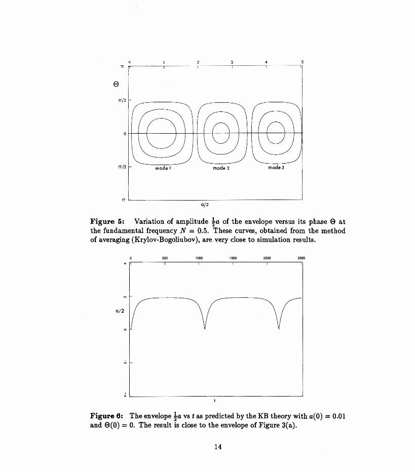
for constant K. The resulting family of curves in the (a, E» plane are shownin Figure 5 for various K. The particular cyclic path followed by the systemdepends on the choice of ~(O). This shows how one can obtain oscillations ofthe type illustrated in Figure 4.

Figure 6 shows a numerical solution of the envelope equations (31) witha(O) = 0.01 and E> = O. The resulting envelope is evidently very close to thesimulation Figure 3a. The envelope equations do not admit a solution witha(O) = 0, but a(O) can be very small, so one can get arbitrarily close to the~(O) = 0 simulation.

The asymptotic analysis thus explains why the resonance like Figure 3a hasan oscillating envelope. For more detail, note that (31) implies, for v = w,

At maximum and minimum a, (31) implies E> = O. Thus

d2a _ £2 J1(a)JiCa) '" { ~.~ as a --+ 0dt2 - v2' a2 0- as a --+ a1

where a1 is the first zero of J1. Thus aCt) has a large positive curvature at itsminimum and a small negative curvature at its maximum. In the case ~(O) = 0,large becomes +00 and small becomes OJ hence Figure 3a.

The peak amplitude a of the oscillations at frequency v and ~(O) 0 isobtained by setting

H(a,O) = 0

This quadratic equation in v has solution

1 1 2 2 1V = 2"w + 2"{w - 8£J1(a)/a }2

Including a < 0 solutions and plotting lal against v gives Figure 7. This showsthe modes obtained in Figures 4 and 5 and how they are modified when v differsfrom w. We see that the higher amplitude modes can exist only within sharply

13

2 3 4n

8

model mode 2 mode3

n/2

rr /2

o~+-+------+-+-++-~~--~+-++-r-r---r-+-i

nk--- ~0/2

5

Figure 5: Variation of amplitude ~a of the envelope versus its phase 0 atthe fundamental frequency N = 0.5. These curves, obtained from the methodof averaging (Krylov-Bogoliubov), are very close to simulation results.

500 1500 20001000

on

~~L ~

2500

Figure 6: The envelope la vs t as predicted by the KB theory with a(O) = 0.01and 0(0) = O. The result is close to the envelope of Figure 3(a).

14

defined intervals of v values centred on w. The width of these intervals decreasesfor large a, like

We have not examined whether or how these modes, other than the lowestamplitude mode, might be excited in a practical situation. They would seemto require a large, abrupt input of energy directly to the ~ motion, when thefrequency is close to w. We know of no mechanism which might achieve this.

5. Conclusions

We have devised and analysed a simplifiedmathematical model ofthe whirlingand thumping phenomenon. The model shows that Hooke universal joints cancause whirling (</> oscillations) in the propshaft at its natural frequency and atovertone and undertone frequencies. The observed thumping at 40kph and 80kphseem likely to correspond to the 2 largest resonances: the fundamental (natural)frequency and its first overtone.

The rubber property in our model is the linear elastic stiffness constant k ofthe bush. There is the obvious dependence of the resonant engine speeds lw, !wand w (radians per second) on k through w = (k / m) t. Increasing stiffness pushesup these speeds. Further, equations (31) show that the thumping frequency (i.e.the envelope frequency) is proportional to e and hence to r/k. So increasingstiffness causes the frequency of thumping to decrease. We note however thatthumping (envelope) frequency is very sensitive to departures from resonantfrequences (Figure 3c) and to initial conditions ~(O) and ~'(O).

The time and data available at the MISG did not permit us to study thiscentral practical problem in more detail; so it remains to find rubber propertiesin the central bush that minimize the severity of the phenomena. However thestudy reported here shows that this problem can be analysed using the followingtechniques.

1. A Lagrangian formulation of the basic dynamics, incorporating more real-istic inertial and gyroscopic terms and rubber parameters.

2. A numerical solution of the resulting differential equations using an IMSLprogram.

3. The iteration scheme of Section 3 to locate resonances of first, second, etcorder.

15

5r-----------------~------------------------~

4

0/2

3

2

mode 3

mode 2

mode 1

0.95

o~ ~ ~ ~ ~0.90 1.101.00

vk»1.05

Fiaure 7: Varia.tion of envelope amplitude la with engine speed ~(O)(= l").Note that models, other than mode 1, are confined to a very narrow range ofengine speeds around the fundamental resonant speed !wo

16

4. The Krylov-Bogoliubov technique (Section 4) to directly obtain the de-pendence of resonant amplitudes and thumping (envelope) frequencies onrubber properties.

These techniques have wide application to problems involving oscillations ofnon-linear systems (Bogoliubov & Metropolski, 1961 and Hagedorn, 1981).

References

Abramowitz, M. and Stegun, I.A. (1965) Handbook of Mathematical Functions.5th edition. New York: Dover.

Bogoliubov, N.N and Metropolski, Y.A. (1961) Asymptotic Methods in theTheory of Non-linear Oscillations. New York: Gordon and Breach.

Hagedorn, P. (1981) Non-linear Oscillations. Oxford: Clarendon.

Prudnikov, A.P., Brychkov, Yu, A. and Marichev, 0.1. (1986) Integrals andSeries Vol I, New York: Gordon and Breach.

Wagner, E.R. and Cooney, C.E. (1979) Cardan and Hooke universal joint. Sec-tion 3.1.1, p39 in Universal Joint and Driveshaft Design Manual. Advancesin Engineering, Series 7. Published by the Society of Automotive Engi-neers, New York.

Zahradka, J. (1973) Torsional vibrations of a non-linear driving system withCardan shafts. J. Sound and Vibration, 26(4), 533-550.

17