9/30/2014

1

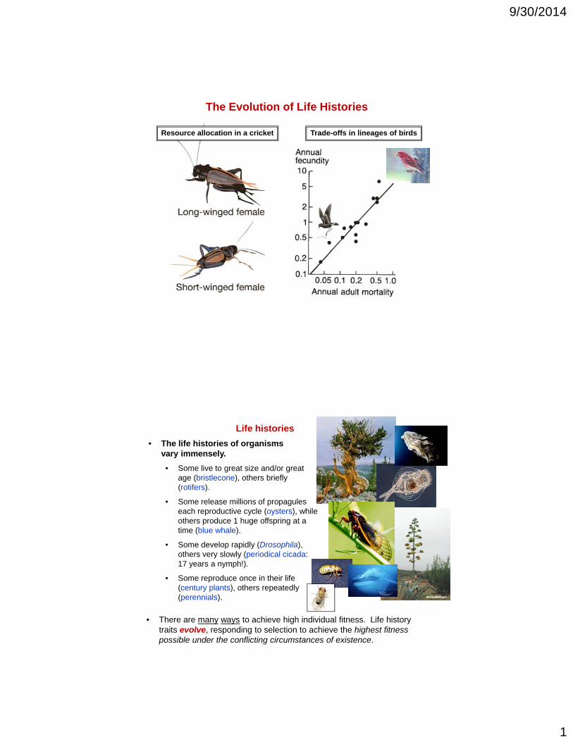
The Evolution of Life Histories

Trade-offs in lineages of birdsResource allocation in a cricket

Life histories

• The life histories of organisms vary immensely.

• Some live to great size and/or great age (bristlecone), others briefly (rotifers).( o e s)

• Some release millions of propagules each reproductive cycle (oysters), while others produce 1 huge offspring at a time (blue whale).

• Some develop rapidly (Drosophila), others very slowly (periodical cicada: 17 years a nymph!).

• Some reproduce once in their life (century plants), others repeatedly (perennials).

• There are many ways to achieve high individual fitness. Life history traits evolve, responding to selection to achieve the highest fitness possible under the conflicting circumstances of existence.

9/30/2014

2

Life history evolution: size, reproduction, aging, and sex ratio

• Life history evolution is all about solutions to the fundamental question of life that all organisms must answer:

How should the newly fertilized zygote (assuming sexual reproduction)

live the life it is about to begin?live the life it is about to begin?

Wikstroemia uva-ursi

mouse

(false Ohelo)

This ultimate question can be broken down into bite-sized pieces:

1. At what age and size should reproduction begin?

2. Should offspring be….

a) few in number but high in quality and large in size, or…b) small and numerous, but less likely to survive on an individual basis?

3 How many times should reproduction occur in a lifetime?3. How many times should reproduction occur in a lifetime?

4. How much energy and time per bout should be allocated to…

a) maintenance,b) growth, and…c) reproduction?

5. Should reproduction be concentrated…

a) early in life with a short lifespan as a consequence, or should…b) less energy be put into each bout accompanied by a longer life?b) less energy be put into each bout, accompanied by a longer life?

6. How many offspring should be male vs. female? And should that decision….

a) depend on ecology or social circumstances?b) be fixed at birth?c) if sequential, start as male and turn female, or vice versa?

9/30/2014

3

Basic life history traits

Life history traits are components of fitness, measured as reproductive success.

Life history traits are those that affect the growth rates of populations. Basic life history traits include:

1. Individual growth, maintenance, and body size.2. Ages at which reproduction begins and ends.3. Number of offspring produced at each age.4. Potential life span.

For semelparous (one-bout) organisms: R = LM

R = reproductive success, or the number of descendants of anR reproductive success, or the number of descendants of an average female after one generation.

L = probability of an average female’s survival to reproductive age.

M = average number of offspring per survivor (fecundity).

Reproductive success in iteroparous species (a simple life table)

x lx mx lxmx

0 1.00 0 0

1 0.75 0 0

2 0 50 4 22 0.50 4 2

3 0.25 8 2

4 0.10 0 0

5 0.00 0 0

3 = R 4

I thi h f l i

R = 3lxmx

x = age

lx = probability of surviving to age x (i.e. proportion of eggs or newborns that survive to age x)

mx = average fecundity (# eggs or newborns) at age x

In this case, each female is replaced, on average, by R = 4 offspring.

This sum is also the growth rate, per generation, of the genotype.

9/30/2014

4

Genetic variation in life-history characteristics in Drosophila serrata from 5 localities in Australia:

Survivorship (fraction of newborns that survive to each age)

bilit

y of

sur

viva

l (l x

)

Fecundity (average egg production per female at each age)

Here, lx (survival rate) and mx (fecundity) are shown for different populations

x =

Pro

ba

for different populations.

These data also imply that life history traits are heritable.

x =

R vs. r

• R is a measure of reproductive success per generation.

• But different genotypes might differ in the length of a generation.

S th th i R it i b tt t hi h i th it• So rather than using R, it is better to use r, which is the per capita rate of population increase per unit time (not per generation).

• But the general analysis just presented gets across the idea, because just like R, r depends on the probability of survival and fecundity at each age.

(not to be confused with r, the coefficient of relatedness…)

9/30/2014

5

Life history evolution: The concept of the trade-off

• Expectation: organisms should evolve ever greater fecundity, ever longer life, ever larger body size, and ever earlier maturity.

• But the ideal organism does not exist. Evolution is the end result of many conflicting forcesof many conflicting forces.

• Example:

• Being large is good – you can have more offspring, both in mass and numbers.

• But it takes time to grow large: You may die before ever reproducing at all!

• Trade-offs are inherent when you must divide up finite resources –a process known as the allocation of resources – among…

• maintenance

• current reproduction

• growth and storage (bet-hedging for future reproduction)

Trade-offs in lineages of birds

(a phylogenetic pattern)

Finch

Petrel

9/30/2014

6

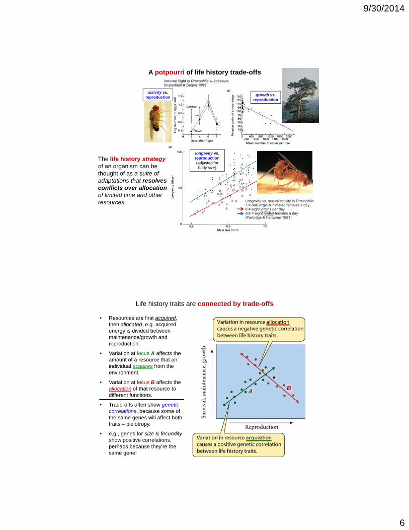
A potpourri of life history trade-offs

growth vs.reproduction

activity vs.reproduction

The life history strategyof an organism can be thought of as a suite of adaptations that resolves

longevity vs.reproduction(adjusted for body size)

adaptations that resolves conflicts over allocation of limited time and other resources.

Life history traits are connected by trade-offs

• Resources are first acquired, then allocated, e.g. acquired energy is divided between maintenance/growth and reproduction.

• Variation at locus A affects the amount of a resource that an individual acquires from the environment.

• Variation at locus B affects the allocation of that resource to different functions.

• Trade-offs often show genetic correlations because some of

A B

correlations, because some of the same genes will affect both traits – pleiotropy.

• e.g., genes for size & fecundityshow positive correlations, perhaps because they’re the same gene!

9/30/2014

7

Optimality in life-history theory: a caveat

• Wherever there are trade-offs, a cost-benefit analysis is appropriate.

• Expectation: Organisms will evolve to the point where the net benefit is maximized – thereby attaining the optimal compromise.

• Normally, such an analysis is straight-forward.

• But cost-benefit, and optimality, assume that when an optimal solution is found, it is optimal for the whole population.

• Not necessarily true – note the useful example of sex ratio:

• If an organism can control the sex ratio of its offspring, then the best ratio depends on the sex ratios produced by other organisms i th l ti Wh ? B th ill b tin the population. Why? Because the rarer sex will be at an advantage. (More on sex ratio later.)

• This is frequency dependence – in this case, negativefrequency dependence.

The concept of optimality, continued.

• So in life history evolution, one has to distinguish between optimality and frequency dependence.

• Optimality = a world at equilibrium.

• Frequency dependence = a changing world; your best strategy depends on what others do.

Example, showing density-dependent selection on rates of increase:

Comparison oftwo genotypes

At very low density, the population growth rate for genotype B is lower than for genotype A.

But genotype B has a selective advantage at high density (Roughgarden 1971).

9/30/2014

8

A short history of life history studies

• Darwin considered life histories, but not a lot.

• Weismann argued for adaptive aging caused by natural (but group) selection – late 1800s.

• A. J. Lotka and R. A. Fisher pioneered life table

A. J. Lotka

R. A. Fisher

analyses – in the 1930s.

• Ten years later: R. Moreau & David Lack on clutch size in birds (Lack’s work stressed an experimental rather than quantitative approach).

• G. C. Williams weighed in (1957 – he was 30) on the evolution of senescence.

• A W F Edwards W A Kolman H Kalmus & C A

D. L. Lack

M. L. Cody A. W. F. Edwards, W. A. Kolman, H. Kalmus & C. A. B. Smith developed treatments of the 1:1 sex ratio (1960; several papers).

• M. L. Cody (1966) applied Richard Levins’ idea of fitness sets to life history evolution, and first spoke of adaptation as the resolution of conflict in allocation of time and energy.

A short history, continued (mostly 1966)

• Also in 1966, Cody introduced the idea that different life history adaptations are favored under high vs. low population density (relative to the carrying capacity – K -- of the environment).

R. H. MacArthur

• These suites were named r-selection and K-selection by Robert MacArthur & E. O. Wilson in The Theory of Island Biogeography (1967).

• G. C. Williams (1966) quantified present and futurecomponents of fitness in the uniform currency of *reproductive value, based on life table calculations.

• Also in 1966, W. D. Hamilton specified the basic scaling forces for natural selection (on fecundity &

E. O. Wilson

scaling forces for natural selection (on fecundity & survival) over the entire life history – see Rose et al. 2007 for a retrospective.

• Reviews in D. Roff (1992), Stephen Stearns (1992), and Brian Charlesworth (1994).Roff

Derek Roff

S. Stearns * The expected reproduction individuals from their current age onward, given that they have survived to their current age. (R. A. Fisher 1930)

9/30/2014

9

Understanding life history traitsThree fields contribute to explaining the evolution of life histories:

I. Demographics: Life history traits depend on population structure – the age, size, and reproductive output of its constituent members.

• For example, selection on reproductive performance is stronger on younger than older adults, because they contribute more to the instantaneous growth rate of the populationrate of the population.

• An increase in mortality at any stage of life devalues older individuals, because those are now less likely to reproduce.

II. Genetics: Life history traits are polygenic – i.e., quantitative traits.

• This means understanding them with quantitative genetic techniques.

• For life history traits to evolve, they must show heritability.

• Depending on h2, a portion of life history variation may be environmental –i h t i ll l ti Thi b d thi i di id li.e., phenotypically plastic. This may be a good thing, so an individual can switch strategies during its lifespan.

III. Phylogenetics: Life histories have evolved in a phylogenetic context.

• As such, comparative methods are appropriate and informative.

• One can tease out constraints or fixed effects due to inheritance of a trait from a common ancestor.

Understanding life history traits I: Demography

Under this heading, we can address a few of those fundamental questions of life.

1. At what age should I start to reproduce?

2. At what size should I start to

a mast year for red oaks

reproduce?

3. How many offspring should I produce at a time?

4. How often should I reproduce during my lifetime?

5. How long should I live?

sexually mature Axolotl

9/30/2014

10

Demography: Age at first reproduction

Because aging – senescence – begins at maturation, the earlier you start reproducing, the better.

• Life is risky. Earlier reproduction means you’re more likely to breed before you die because of some environmental hazard, e.g. y , gpredation, disease, or accident.

• Earlier reproduction also shortens the generation time, so the individual’s contribution to population growth is greater when it starts breeding at a younger age.

• Advantage of early reproduction is further enhanced if the population size is increasing rather than decreasing, because each individual born today is a larger fraction of the total population than an i di id l b i h findividual born in the future.

Note the difference in lx between ages 2 and 3

x lx mx lxmx

0 1.00 0 0

1 0.75 0 0

2 0 50 4 2 R !2 0.50 4 2

3 0.25 8 2

4 0.10 0 0

5 0.00 0 0

3 = R 4

R = 3lxmx

same R !(contribution to population growth)

x = age

lx = probability of surviving to age x (i.e. proportion of eggs or newborns that survive to age x)

mx = average fecundity (# eggs or newborns) at age x

9/30/2014

11

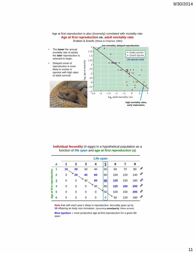
Age at first reproduction is also (inversely) correlated with mortality rate.Age at first reproduction vs. adult mortality rate:

Snakes & lizards (Shine & Charnov 1992)

• The lower the annual mortality rate of adults, the later reproduction is

low mortality, delayed reproduction

selected to begin.

• Delayed onset of reproduction is most likely to evolve in species with high rates of adult survival.

(16 species total)

high mortality rates, early maturation.

Individual fecundity (# eggs) in a hypothetical population as a function of life span and age at first reproduction (a)

Life span

a 1 2 3 4 5 6 7 8

1 10 20 30 40 50 60 70 80

2 0 20 40 60 80 100 120 140

3 0 0 30 60 90 120 150 180

4 0 0 0 40 80 120 160 200

5 0 0 0 0 50 100 150 200

ge

at f

irst

rep

rod

uct

ion

6 0 0 0 0 0 60 120 180

Note that with each year’s delay in reproduction, fecundity goes up by 10 offspring as body size increases. (assuming semelparity; follow arrows)

Blue typeface = most productive age-at-first-reproduction for a given life span.

Ag

9/30/2014

12

Demography: Size at first reproduction

Generally, the bigger you are when you first reproduce, the better.

1. You can produce a larger number of offspring.

• Larger mass means more offspring at a time – larger organisms are more fecund.

2. You can provide better parental care. Larger size means…

• more nutrients to the unborn, as yolk or larger propagule size,• easier acquisition of more resources for your young,• and better protection for your young.

3. You can be better at intra- and intersexual competition. Larger size means…

• winning contests with other males,• and attracting females by virtue of your ‘handicap’.

Small organisms are not small because it improves fecundity or lowers mortality. They are small because it takes time to grow large, and with heavy mortality, the investment in growth would never be paid back in increased fecundity.

Size at first reproduction

Example from the sea lion Zalophus californianus, which has a harem-style mating system

Males weigh in at 600 lbs. and mature at age 11 or 12.

If a male tries to secure a harem at a smaller size, he will

Females are much smaller than males (200 lbs), and become sexually mature at 5 or 6 years of age.

fail, and likely be killed as well.

9/30/2014

13

Size vs. age in conflict Parental care vs.age of mother

• Sea lion: size and age (at first reproduction) are in conflict.

• larger size requires time• larger size requires time later start to reproduction.

• So despite the advantages of early reproduction, there are benefits to delayed maturation.

This does NOT mean that the optimal age of reproduction is 30. Rather, it is somewhere between 15 & 30 – a compromise between early reproduction and the experience of age.

Selection can change life-history optima:

• For body size evolution, there are optimal solutions to mandatory trade-offs.

• Marine iguanas (like the sea lions):

Marine iguanas on different islands

1. Assume that something, like too little food, is selecting against larger male sea lions.

2. That will favor breeding by the smaller males.

3. And that could eventually produce earlier maturation of individuals in that population.

4. In other words, the favored life-history strategy will depend upon what others in the population are doing. Strategies will change.

9/30/2014

14

Understanding life history traits I: Demography

1. At what age should I start to reproduce (earlier or later)?

2. At what size should I start to reproduce (small size or large size?p ( g

3. How many offspring should I produce at a time? (includes propagule number and propagule size)

4. How often should I reproduce during my lifetime (once or many)?

5. How long should I live?

Demography: Fecundity

Even though “more is better,” there are also life-history “decisions” to be made about the number vs. size of offspring.

1. Numerous, tiny offspring might be produced under conditions of extremely high, unavoidable risk very early in life (r-selection).

M l t d ti l th t j it f hi h ill• Many plants produce tiny propagules, the vast majority of which will never live to reproduce. The parent ‘floods’ the environment in order to produce a few successful offspring.

• most mortality results from “non-selective deaths” (accidents)

• Another example: Oysters (and many other bivalve species) produce millions of eggs/zygotes, of which only a few will find a favorable place to settle.

Crassostrea gigasCrassostrea gigas oyster larvae

9/30/2014

15

Fecundity

2. Few, but large, offspring are favored by selection under more stable, predictable environmental conditions (K-selection).

• Parental care: mother (or father) invests resources such as food and protection in larger, better developed, but fewer young.and protection in larger, better developed, but fewer young.

• Even insects: the tsetse fly of Africa (Glossina spp.), which is a live bearer of one offspring at a time.

tsetse fly(22 species)

Numbers vs. Quality: you can’t have both at the same time

Allocation trade-off in 26 families of fishes(Elgar 1990)

The same, in Drosophilaspecies (Berrigan 1991)

big eggs,small clutches

big eggs,small clutches

9/30/2014

16

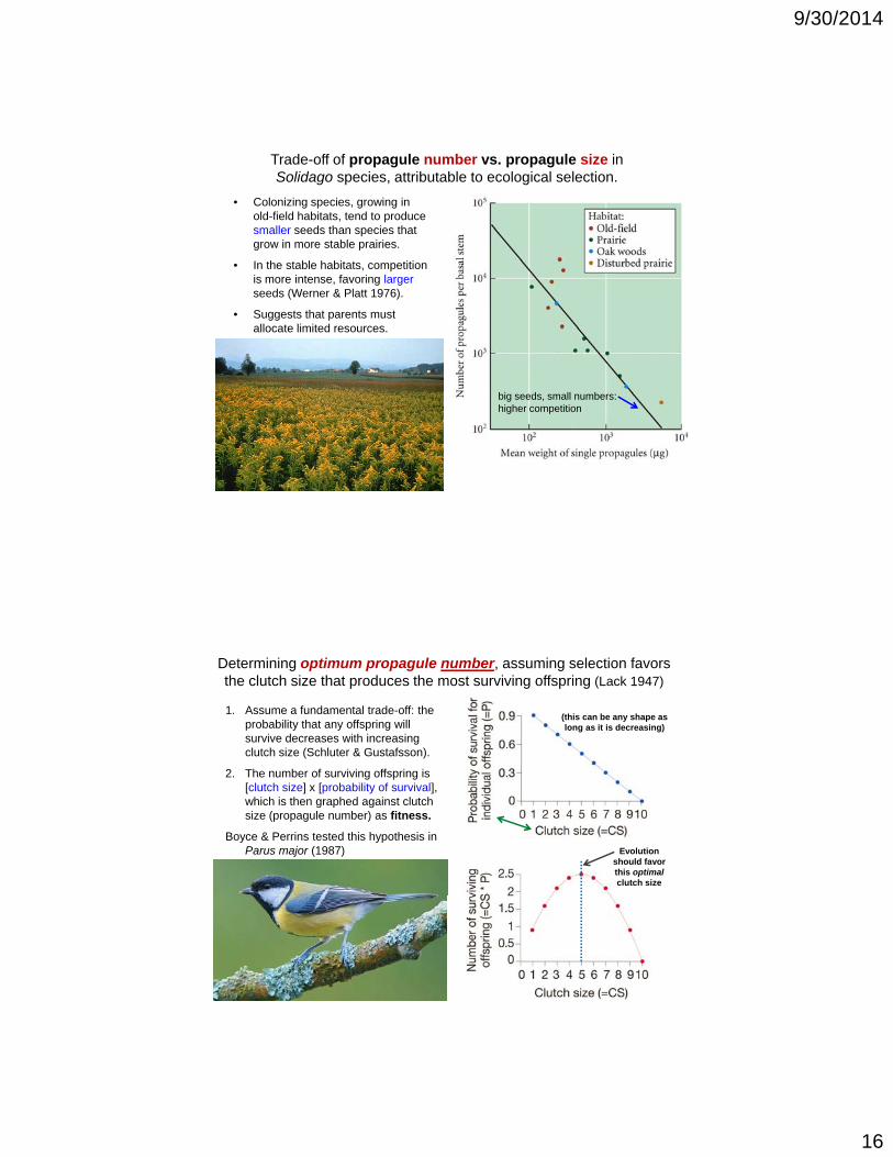
Trade-off of propagule number vs. propagule size inSolidago species, attributable to ecological selection.

• Colonizing species, growing in old-field habitats, tend to produce smaller seeds than species that grow in more stable prairies.

• In the stable habitats, competition is more intense, favoring largerseeds (Werner & Platt 1976).

• Suggests that parents must allocate limited resources.

big seeds, small numbers:higher competition

1. Assume a fundamental trade-off: the probability that any offspring will survive decreases with increasing clutch size (Schluter & Gustafsson).

Determining optimum propagule number, assuming selection favors the clutch size that produces the most surviving offspring (Lack 1947)

(this can be any shape as long as it is decreasing)

2. The number of surviving offspring is [clutch size] x [probability of survival], which is then graphed against clutch size (propagule number) as fitness.

Boyce & Perrins tested this hypothesis in Parus major (1987) Evolution

should favor this optimal clutch size

9/30/2014

17

Testing Lack’s hypothesisin Parus major in Wytham Wood

8.53

12 (optimal clutch size)

DavidLack

• Data collected from 4,489 clutches monitored from 1960 to 1982 were inconsistent with Lack’s hypothesis.

Eggs added/removedfrom mother’s clutch

• average clutch size = 8.53…• but the best offspring survival occurred in clutches of 12 eggs

• Explanation: an additional trade-off is operating, between a mother’s clutch size in the first year and her clutch size in future years [not shown].

• In addition, females reared in nests with smaller clutches had higher reproductive success (Schluter & Gustafsson 1993).

Also, note extensive year-to-year variation (Boyce & Perrins 1987)

8.53 12

9/30/2014

18

Another example: number of inflorescences in two consecutive years

• The turf-grass, Poa annua

• The two colors of symbols represent plants from two different habitats, grown together.

Th lt d t t th t d on

dse

aso

n Trade-off:

• The results demonstrate the trade-off, plus a genetic basis for cost of reproduction – the two populations differ (Law 1979).

ore

scen

ces

per

pla

nt

in s

eco

Nu

mb

er o

f in

flo

Number of inflorescences per plant in first season

0 300 600

Determining the optimum propagule size, based on the

number/size trade-off vs. survival.

1. Assume a trade-off between size and number of offspring (a).

2. Assume also that individual offspring

1. Trade-off

(a)

(b)2. Assume also that individual offspring will survive better if they are larger (b).

3. [Of course the survival probability cannot exceed unity (b)]

4. Expected fitness (c) is [number of offspring] x [probability of survival].

5. Graph the expected fitness against propagule size (c).

2. Offspring survival

1.0(b)

(c)6. In this case, increasingly large

offspring get progressively smaller survival benefit, so intermediate size gives the highest parental fitness.

(Theory by Smith & Fretwell 1974)

3. Optimal size of offspring

Evolution should favor this optimal clutch size

9/30/2014

19

Demography: Number of cycles of reproduction

• An organism can reproduce once, or many times in its lifetime.

• Once = semelparity (includes “annual” and “big-bang” life cycles).

• Multiple bouts = iteroparity (includes “perennial” life cycles)

• Expectation: many bouts of reproduction (iteroparity) is better. But selection pulls organisms in many directions.

• In general, an organism will be selected to engage in additional bouts of reproduction only if it is likely to survive the first bout.

• If so, it will be selected to invest less in the first bout in anticipation of future reproduction – the iteroparous (bet-hedging) strategy.

S th b f l f d ti i

cocklebur

joe pye weed• So the number of cycles of reproduction is a

consequence of simultaneous interactions (including trade-offs) among such factors as:

(i) harshness of the environment

(ii) mating opportunity

(iii) life span.