Resource curse or not:

A question of appropriability∗

Anne D. Boschini†, Jan Pettersson‡ and Jesper Roine§

December 2005

Abstract

This paper shows that whether natural resources are good or bad for a country’sdevelopment crucially depends on the interaction between institutional setting andthe type of resources possessed by the country. Some natural resources are, foreconomical and technical reasons, more likely to cause problems such as rent-seekingand conflicts than others. This potential problem can, however, be countered bygood institutional quality. In contrast to the traditional resource curse hypothesis,we show the impact of natural resources on economic growth to be non-monotonicin institutional quality. Countries rich in minerals are cursed only if they have lowquality institutions, while the curse is reversed if institutions are sufficiently good.

Keywords: Natural Resources, Appropriability, Property Rights, Institutions,Economic Growth, Development

JEL: O40, O57, P16, O13, N50

∗The authors wish to thank Oriana Bandiera, Mark McGillivray, Per Pettersson Lidbom, SilviaPezzini, Peter Skogman Thoursie and Fabrizio Zilibotti for insightful comments and discussions. Wealso thank seminar participants at Stockholm School of Economics, Stockholm University, Uppsala Uni-versity, and the EEA Annual Meeting (Madrid, 2004). Financial support from Jan Wallander’s and TomHedelius’ Foundation is gratefully acknowledged.

†Corresponding author: Anne Boschini, Department of Economics, Stockholm University, S-106 91Stockholm, Sweden. E-mail: anne.boschini@ne.su.se

‡Department of Economics, Stockholm University§Department of Economics, Stockholm School of Economics

1

1 Introduction

A major puzzle in economic development is the existence of a negative correlation between

economic growth and large natural resources. Some of the fastest growing economies over

the last few decades are countries with very little natural wealth (such as Hong Kong,

Singapore, Korea, and Taiwan), whereas some of the poorest economic performers (like

Angola, Sierra Leone, and the Democratic Republic of Congo) are countries with enormous

resources. A number of recent studies have concluded that the negative relationship

between resource abundance and growth also holds for large samples of countries after

controlling for other relevant characteristics.1 This relationship, the so called ’resource

curse’, has become widely accepted as one of the stylized facts of our times.2

However, the resource curse seems far from inevitable. While oil appears to have been

the cause of recurrent problems in countries like Venezuela and Ecuador, Norway has

become one of the world’s richest economies largely thanks to its oil endowments. The

possession of diamonds has arguably been disastrous for the development of countries

like Sierra Leone, Liberia and the Democratic Republic of Congo. However, this does

not seem be the case in countries like Australia, South Africa or Botswana – one of the

world’s fastest growing economies over the past thirty years. There are several examples

of countries rich in similar resources that have experienced extremely different economic

growth. Studying the examples in Table 1, it seems that for every catastrophic failure

there is a counter example of success.

In this paper, we show that the effect of natural resources on economic development

is not determined by resource endowments alone, but rather by the interaction between

the type of resources that a country possesses, and the quality of its institutions. This

combination of factors determines what we call the appropriability of a resource. The

concept of appropriability captures the likelihood that natural resources lead to rent-

1E.g. Sachs and Warner (1995); Gylfason et al. (1999); Leite and Weidmann (1999). Ross (1999)provides an overview of much of this literature.

2Wright (2001, p. 1)

2

seeking, corruption or conflicts which, in turn, harm economic development. We will

show that in countries where resources are highly appropriable - as determined by the

type of resources as well as institutional quality - resource abundance is problematic,

while in countries where resources are less appropriable, they can contribute to economic

growth.

Table 1: Relative growth performance in ten resource rich economies

Growth Main resourcea Institutional1975-1998 qualityb

Botswana 4.99 Diamonds 0.706Chile 3.71 Copper 0.668Norway 2.82 Crude Petrol 0.966Australia 1.97 Minerals 0.932Canada 1.73 Minerals 0.974Sample Average 1.53 0.638Ecuador -0.79 Crude Petrol 0.592Niger -1.45 Minerals 0.520Zambia -1.94 Copper 0.434Sierra Leone -2.05 Diamonds 0.406Congo, Democratic Rep. -5.39 Ores and Metals 0.232

a The listing of main resources is based on UNCTAD data on export structure in 1975.b The measure of institutional quality is a ”Property Rights Index” based on data from

Keefer and Knack (2002). The index score for a country is between zero and one wherehigher scores mean better institutional quality. See Appendix Table A2 for details.

It is important to stress the two dimensions of our concept. On the one hand, cer-

tain resources are, by their physical and economical characteristics, more likely to cause

appropriative behavior. Resources which are very valuable, can be stored, are easily

transported (or smuggled), and are easily sold are, for obvious reasons, more attractive

to anyone interested in short-term illegitimate gains. This suggests that resources such

as diamonds or precious metals are more problematic than, say, agricultural products.3

On the other hand, this does not mean that all countries with potentially problematic

types of resources will suffer, while others will do fine. The potential problem of having

certain types of resources can be countered by having good institutions. Given the right

3Indeed, many case studies of development failure and resource abundance are concerned with mineralrich countries, rather than countries rich in natural resources in general. Campbell (2002) deals withconflict diamonds, Karl (1997) gives examples of problems related to oil, and Auty (1993) studies countriesdependent on non-ferrous metals.

3

institutional framework, finding oil or diamonds has the potential of boosting a coun-

try’s economic development, while the same resources are likely to lead to problems in a

country with poor institutions.

Consider the cases of Ecuador and Norway: in 1967 and 1969, respectively, these coun-

tries discovered unexpectedly vast amounts of oil, which have ever since constituted an

important share of their GDP.4 In terms of institutional setting, however, these countries

were very different. Ecuador had just ended a short period of military government, which

was to return in 1972. Norway on the other hand was one of the worlds oldest democracies

with firmly established institutions. At the time of the oil discoveries, the institutional

gap between Ecuador and Norway was thus definitely to Ecuador’s disadvantage. Accord-

ing to the hypothesis suggested in this paper, Ecuador would be expected to have more

difficulties than Norway in transforming the oil revenues into long-term development. In

the past decades the yearly growth rate of the Norwegian economy has been on average

seven times higher than that of Ecuador.

Diamonds perhaps stand out as the most potentially problematic type of resources

in their extreme value (per unit) and the ease with which they can be smuggled. When

it comes to the ease of extraction, it is important to distinguish between primary (kim-

berlitic) diamonds, which require costly mining technology, and secondary (alluvial) di-

amonds, for which the extraction costs are virtually zero. Mining of primary diamonds

requires large investments and therefore good property rights protection is essential for

such investments to be undertaken. The insecure property rights in a country like Tan-

zania, which is known to have large amounts of kimberlitic pipe, have made it difficult

to attract investors and therefore this natural endowment has not enhanced its economic

growth. On the other hand, a country like Botswana, which has a higher institutional

quality than the world average, has successfully exploited its kimberlitic diamond re-

sources over the past thirty years. The same is true for Australia, which quickly managed

4According to our own calculations based on figures from World Development Indicators, oil hasconstituted 10 to 15 per cent of GDP in both Ecuador and Norway between the late 1970s and 2000.

4

to turn its recent diamond findings (during the 1980s) into a source of income.

When it comes to alluvial diamonds these are known to be very problematic in the

absence of good institutions. The civil wars in Angola, the Democratic Republic of Congo

and Sierra Leone are, for example, to a large extent fuelled and sustained by illegal

trade in diamonds.5 However, alluvial diamonds have not caused problems everywhere.

First discovered in 1867, South Africa has had large deposits of alluvial diamonds.6 The

economic effects of these findings as compared to the discoveries in Sierra Leone in 1930

have arguably been very different. But so have institutions. While both countries were

British colonies, the Cape Colony, which later expanded and eventually became South

Africa, obtained representative government with two elected houses as early as 1854.

Sierra Leone on the other hand, had the lowest colonial status in the British Empire, and

it was not until the 1950s that Sierra Leone started to have any form of representative

institutions. While the diamond findings in South Africa quickly drew investors and

became an industry with firm property rights, the same resource in Sierra Leone largely

remained up-for-grabs and has been a problem ever since it was found.7

In the following we will show that the economic impact of resource endowments sys-

tematically depends on the interaction between the types of resources and a country’s

institutions. In Section 2 we will relate our ideas to previous writings on the effects of

resource abundance on economic development. In Section 3, we specify our hypothesis

and present our data. In particular, we report how we have constructed our measure for

the most appropriable resources. Section 4 tests our hypothesis using OLS regressions

5Campbell (2002) gives a full account of the devastating consequences of illicit diamonds in SierraLeone. Recently the UN as well as the World Diamond Council (WDC) have recognised these problemsand started projects to try to stop the illegal diamond trade.

6Even though South Africa has very large alluvial deposits, the main sources of diamond are kimber-litic.

7This description of institutions in these countries is clearly very simplistic. In the early 20th centurythe Cape colony lost some of its representative institutions and later came to limit franchise and politicalrights only to the white population. Regarding Sierra Leone, it was not a colony for which Britainhad ever sought, but rather one they had to take on. Sierra Leone eventually obtained the status ofProtectorate in 1895, which meant minimal British administrative and political arrangements combinedwith actions to prevent crime and lawlessness. For more details see the Oxford History of the BritishEmpire (2001).

5

of GDP growth on different measures of natural resources, institutions and their inter-

actions. We also address the issue of endogenous institutions and run 2SLS regressions

instrumenting for institutional quality. In Section 5 we check the robustness of our results

with respect to influential observations, sample size, the influence of armed conflicts and

the choice of institutional variables. Section 6 concludes.

2 Related literature

There is strong evidence that resource abundant countries have had lower average growth

rates in the Post-war period as compared to their resource-poor counterparts. However,

there seems to be little agreement on why this relationship exists. The different theories

that have been advanced can usefully be grouped into economic and political-economy

explanations.8

Most of the recent economic explanations are versions of the so called ”Dutch Dis-

ease”.9 The basic argument in these models is that windfall gains from natural resources

(either through sudden increases in the price of the resource, or through the discovery of

new resources) have a crowding-out effect on other sectors of the economy. For example,

in Sachs and Warner (1995), following Matsuyama (1992), positive externalities in the

form of learning-by-doing are assumed to only be present in the manufacturing sector of

the economy. This implies that the larger is the natural resource sector (and the smaller

is the manufacturing sector), the smaller is the positive externality feeding the growth

process. However, these theories typically predict that the effect of natural resources

on growth should unambiguously be negative: the more natural wealth, the worse the

outcome. As such, these theories cannot explain why Botswana and Norway have been

8One could, of course, add ”pure” political explanations, such as the ”rentier effects” and (anti)”modernization effects” (see Ross (2001) for a discussion of these) as well as sociological studies ofnegative effects of resources on development (see Ross, 1999, footnote 2).

9For example, Corden and Neary (1982); Neary and van Wijnbergen (1986) and Krugman (1987).For other economic theories based on, for example, declines in terms-of-trade and sensitivity to volatilecommodity prices, see the overview in Ross (1999).

6

successful, while Sierra Leone and Ecuador have not.10

A number of papers have put forward more politico-economic explanations for why

natural resources have negative effects on growth. Lane and Tornell (1999) and Torvik

(2002) have developed theoretical models of rent-seeking where resource abundance in-

creases the incentives to engage in ”non-productive” activities to capture the rents from

the resources. Even though these papers certainly give important insights, they also

predict a monotone adverse effect of natural resources on economic growth. Collier and

Hoeffler (1998, 2002a) point to resources as a source of armed conflict. They find a non-

linear relationship between natural resources and the risk of armed conflicts, but they still

do not explain why some resource rich countries prosper whereas others fail.11

Auty (1997); Woolcook et al. (2001) and Isham et al. (2003) have – as we do in this

paper – stressed the importance of different types of resources. What they term ”point

source” resources, such as plantation crops and minerals, are more likely to cause problems

than ”diffuse” natural resources, such as rice, wheat and animals. These theories provide

predictions on why different resource-rich countries may be affected differently by their

natural wealth. Those with plantation crops, oil or diamonds are more likely to have

bad outcomes than those with rice, wheat, and livestock. This prediction seems to be

supported by data. However, these theories cannot account for the facts in Table 1. Why

is it that when comparing countries with similar natural resources, some seem to gain

from their endowments when others lose? The reason we suggest is that the relationship

between natural resources and growth is non-monotonic in institutional quality. Relating

to the theories of resources as a source of rent-seeking or conflict, the idea is that better

10In Gelb (1988) several studies find that the mechanisms suggested by these models were not there inthe data. Resource booms have not shifted capital and labour away from manufacturing. Furthermoregovernments seemed to be able to counter the ”disease” if necessary. As concluded by Neary and vanWijnbergen (1986): ”In so far as one general conclusion can be drawn it is that a country’s economicperformance following a resource boom depends to a considerable extent on the policies followed by itsgovernment...”.

11Given the insights on the importance of conflicts from Collier and Hoeffler (1998, 2002a) we controlfor this and show that our results are not purely driven by resources causing conflict and thereby harminggrowth.

7

institutions increase the costs of non-productive activities.12 Merging these with theories

suggesting that types of resources matter, we also claim that the non-monotonicity will

depend on what resources the country is rich in. Specifically, our prediction is that

institutional quality is most crucial for countries rich in diamonds and precious metals.

Such countries, which have poor institutions, are expected to have the largest negative

effects of resources, while similar countries with good institutions are predicted to have

large gains from these.

In emphasizing the interaction between types of resources and institutions we face the

crucial issue of potential endogeneity of institutions with respect to resources. As shown by

Engerman and Sokoloff (2002), the differences in initial factor endowments between North

and South America have played an important role in shaping the different institutions.

Put simply, their argument is that some countries enjoyed conditions favorable for growing

crops, such as sugar, which were most efficiently produced on large plantations. This led

to concentrations of wealth, political power, and human capital, and in the long run to

worse economic outcomes. In similar spirit, Acemoglu et al. (2002) argue that initial

conditions shaped the types of institutions set up in areas colonized by Europeans. They

suggest that ”extractive institutions” were set up where large gains could be made from

extractive policies and where settlement was difficult due to the disease environment.

These areas were often densely-settled and initially relatively rich. ”Institutions of private

property”, on the other hand, were set up in places where Europeans settled in large

numbers, which were often poor and sparsely populated at the time of settlement. These

institutional differences later came to determine which areas could take advantage of the

opportunities to industrialize.13 Easterly and Levine (2002) and Rodrik et al. (2002) go

as far as to argue that once institutional quality is controlled for there is no separate

effect from ”geographical factors”. While there is no doubt that geographical factors in

12This idea echoes Rodrik (1999), who stresses the role of institutions of conflict management.13Acemoglu et al. (2001) specifically argue for the importance of settler mortality in shaping early

institutions which, through the persistence in institutional quality, has come to produce different long-run economic outcomes.

8

general, and resource endowments in particular, have played an important role in shaping

institutions, this does not imply that all resources which are relevant today have been

part of this development. In some cases institutional differences precede the discovery of

resources and consequently determine the effect of these discoveries on the economy. For

example, at the time of the oil discoveries in Norway and Ecuador, these countries had very

different institutions, and we would argue that these differences determined the diverse

impacts of these discoveries on the economy. The same is true for many other countries

and resources. Nevertheless, there is a potential endogeneity problem and therefore, we

address the possibility of institutions being endogenous and show that our results hold

when instrumenting for institutional quality.

In closely related and independent work, Mehlum et al. (2002) and Robinson et al.

(2002) share our prediction of resources being non-monotonic in institutional quality.

Mehlum et al. (2002) develop a model where entrepreneurs choose between becoming ”pro-

ducers” or ”grabbers”. The relative payoff from these activities depends on how ”grabber

friendly” the institutions are, which also determines the effect of natural resources on the

economy. More natural resources raise the national income if institutions are ”produc-

tion friendly”, but reduce the national income if they are ”grabber friendly”. Robinson

et al. (2002) develop a model with similar predictions regarding the non-monotonic ef-

fect of resources depending on institutional quality, but where instead political incentives

generated by resources are key. In countries with good institutions resources are pos-

itive because the perverse political incentives are mitigated, but in countries with bad

institutions resources remain a curse.

Our study could be viewed as a test of these theories and we will indeed show that the

effect of resources on economic performance depends on institutional quality. But we do

not test whether the channel is through the misallocation of talent between productive

activities and rent-seeking, through perverse political incentives, or through conflict over

resources. The reason is that we believe all these channels to be important and affected

9

by institutional quality in similar ways. Instead we add the dimension of resource type to

our analysis and show that how much institutions change the impact of resources crucially

depends on the type of resources a country has.

3 Our hypothesis and data

In contrast to the standard resource curse, our basic hypothesis is the following: Natural

resource abundance is negative for economic development only if the country lacks the

proper institutions for dealing with the potential conflicts and the rent-seeking behavior

in which the resources may otherwise result. A lack of proper institutions is likely to be

more serious for countries rich in physically and economically appropriable resources.

Figure 1: The two dimensions of resource appropriability. The number adjacent to eachcountry name is the share of primary exports in GDP in 1971. See the text for details.

Plotting countries with respect to the two dimensions of resource appropriability can

10

serve as a simple illustration of our theory. Figure 1 shows a number of countries with

similar shares of primary exports in GDP (a common proxy for natural resources) graphed

with respect to type of resource and institutional quality.14 In the first and fourth quad-

rant are countries with type of resources that are potentially problematic in that they are

more likely to cause appropriative behavior (than those in the second and third quad-

rant).15 Those on the left-hand side of the y-axis have lower than average measures of

institutional quality, while those on the right-hand side have better than average insti-

tutions.16 According to any theory which emphasizes the share of primary exports as

important for economic performance, the contribution from resources to economic growth

should, ceteris paribus, be roughly the same for all these countries.

Our prediction is that countries in the first quadrant will benefit from their natural

wealth, while those in the fourth quadrant will instead be ”cursed” by their endowments.

For countries in the second and third quadrant - countries with less appropriable types of

resources - the effects of the interaction between natural resources and institutions are less

instrumental for economic development. This can be stated as two separate hypotheses.

The institutional dimension of appropriability: Natural resource abundance is neg-

14The countries included are all those in our data set with shares of primary export in GDP between0.05 and 0.20. The average value for the respective quadrants is 0.11 for the first, 0.14 for the second,0.11 for the third and 0.13 for the fourth quadrant. This means that in terms of this proxy for naturalresource wealth the countries in the respective quadrants are, on average, very similar.

15Countries are classified according to their three leading primary exports in 1975. The lead export isthe main determinant of the country’s position in the graph and the second and third most importantprimary product determine the ”direction” in which the country is placed. In Brazil and Thailand, forexample, sugar is the lead export product. But in Brazil the second and third export products are coffeeand iron ore, while in Thailand they are rice and maize, so Brazil is moved up toward minerals relative tothe heading ”coffee, cocoa, sugar and timber”, while Thailand is moved down toward agriculture products.Some countries, such as Australia, are dominated by relatively equal shares of minerals and agriculturalproducts and are therefore positioned in between these labels. Exactly how these natural resourcesshould be ranked in terms of technical appropriability is, of course, debatable. In our analysis, we willonly distinguish between a broad measure of natural resources (which includes all primary products)and narrower measures of more appropriable resources which only include ores and metals, and an evennarrower measure of what we define as the most appropriable resources, only including precious metalsand diamonds. See Auty (1997) and Woolcook et al. (2001) for a slightly different distinction betweentypes of resources.

16Institutional quality is measured as an (unweighted) average of indexes for the quality of the bu-reaucracy, corruption in government, rule of law, the risk of expropriation of private investment andrepudiation of contracts by the government. See Appendix Table A2 for details.

11

ative for economic development only under poor institutions.

The technical dimension of appropriability: The impact of institutional quality and

abundant natural resources is more pronounced, the more technically appropriable are the

country’s natural resources.

The basic econometric specification for testing the proposed effects of resources and

institutions in country i becomes

growthi = X ′

iα + β1NRi + β2Insti + β3(NRi × Insti) + εi , (3.1)

where growth is the average yearly growth rate of GDP, X is a vector of controls including

initial GDP per capita level, period averages of openness and investment ratios, dummy

variables for Sub Saharan Africa and Latin America respectively and a constant. NR is

a measure of natural resource wealth (for which we will use our four measures discussed

below) and Inst is our measure of institutional quality. NR × Inst is the interaction

between natural resources and institutional quality.

According to our first hypothesis β1 should be negative (the standard resource curse

finding), β2 should be positive (the standard finding that good institutional quality is

beneficial for growth) and β3, the coefficient for the interaction between natural resources

should be positive and - if it is to reverse the resource curse - have an absolute value larger

than β1.17 This would mean that as long as the institutional quality is good enough,

natural resources will have a positive net effect on economic growth. Furthermore, our

second hypothesis implies that the impact on the growth rate of GDP of both the negative

effect of the resources themselves (β1) and the interaction with institutional quality (β3)

should be stronger, the more appropriable are resources and the weaker are institutions.

Put differently, the institutional quality is more important for countries rich in technically

appropriable resources than for others.

17The fact that our measure of institutional quality has been rescaled to a 0-1 measure allows us todirectly compare the coefficients.

12

When addressing our second hypothesis, we are limited by the availability of data

for all natural resource measures for each country. This leaves us with a sample of 80

countries, both industrialized and developing (see Appendix Table A1 for a complete

listing). Our dependent variable, growth, is defined as the average yearly growth rate of

GDP between 1975 and 1998.

We use four different measures of natural resources to capture a gradual increase

in physical and economical appropriability. As the broadest measure we use the share

of primary exports to GNP from Sachs and Warner (1995), PrimExp (by them labelled

SXP ). In terms of appropriability this measure includes everything from meat to precious

metals, that is the whole range of the y-axis in Figure 1. Second broadest is OrMetExp,

which includes the exports of ores and metals as a share of GDP – this corresponds to the

upper half of the y-axis. A similar measure in terms of appropriability is MinProd, the

share of mineral production in GNP.18 This differs in two respects, however. It does not

include ores and it is a production – not an export – measure. If technically appropriable

resources are likely to be diverted on their way from production to export, this proxy is

expected to contain less measurement error.

Our fourth, and narrowest, measure MidasProd is the value of production of gold,

silver, and diamonds (industrial as well as gem stone) as a share of GDP – that is, the very

top of the y-axis in Figure 1. This measure is based on a combination of production and

price data. Production data are from the Minerals Yearbook, where production is reported

in volumes. For price data on silver and gold, we employ average yearly market prices

reported by the U.S. Geological Survey (1999). Such prices do not exist for diamonds

because of the large variation in quality. What we do have is the U.S. import quantities

and values of diamonds (industrial and gem stone) from different countries. These are

used to obtain the per carat price for each country and quality, which we multiply with

production data. The total value of gold, silver and diamonds for each country is divided

18This measure is also taken from Sachs and Warner (1995), where it is called SNR.

13

by GDP to obtain MidasProd.19

To reduce the risk of reverse causality we use initial year measures for all four resource

proxies.20 To capture institutional quality we employ the (unweighted) average of indexes

for the quality of the bureaucracy, corruption in government, rule of law, the risk of

expropriation of private investment, and repudiation of contracts by the government from

Keefer and Knack (2002). Our control variables are the level of GDP per capita in

1975, investment and trade openness.21 Sources and exact definitions of all variables are

presented in Appendix Table A2. Table 2 reports the correlations between these main

variables and enables us to address a number of issues. First, it indicates that the measures

of natural resources in themselves are not proxies for a country’s level of development.

In fact, the correlation between per capita GDP in 1975 and the different measures of

natural resources is fairly low. Moreover, this potential problem seems to be largest for

the broadest measure of natural resources (PrimExp), while the narrower measures are

less correlated with the GDP level. Second, in Table 2, we find institutions to be quite

modestly (negatively) correlated with the measures of natural resources. Third, Table 2

reports the initial GDP level and investments to be highly correlated with institutions.

This is addressed in the robustness section.

19The net value of alluvial diamonds is clearly higher (due to lower extraction costs) than that ofkimberlitic diamonds. However, we cannot distinguish between different production costs for any naturalresource and therefore, we use the export value of the respective resources.

20The exception is MidasProd. Due to heavy price volatility during the years surrounding 1975, weuse the average of 1972, 1974, 1976, 1978 and 1980, to avoid the choice of a specific starting year toinfluence our results. Our findings are similar when using MidasProd for 1974 or 1976, however.

21One control variable we have excluded is average years of schooling in the population, since it ishighly correlated with the other control variables. The regression results are robust to the inclusion ofschooling, however.

14

Table 2: Correlation matrix for the entire sample

Growth Inst Prim OrMet Min Midas GDP75 OpenInstitutions 0.39* 1PrimExp -0.34* -0.29* 1OrMetExp -0.14 -0.12 0.47* 1MinProd -0.45* -0.33* 0.40* 0.42* 1MidasProd -0.03 -0.07 -0.02 0.31* 0.30* 1GDP75 0.19 0.83* -0.31* -0.17 -0.22 -0.14 1Openness 0.23 0.17 0.30* 0.30* -0.01 0.03 0.08 1Investments 0.55* 0.73* -0.31* -0.11 -0.31* -0.15 0.69* 0.30*

Figures in bold denote significance at least at the 10 per cent level; * at the one per cent level.

4 Main results

To test our hypotheses, we first run regressions using the broadest measure of natural

resources (PrimExp). Then, we use gradually narrower definitions of natural resources,

letting the measure of resources include fewer, but more physically and economically ap-

propriable resources. If more appropriable resources are better for economic development

when institutional quality is good, as well as increasingly problematic when institutions

are bad, this should appear in the regression outcomes. As the measure of natural re-

sources narrows down toward more technically appropriable resources, we expect the

(negative) effect of resources (β1) as well as the (positive) effect of the interaction term

(β3) to be more pronounced.

Columns (1)-(4) in Table 3 show our main results. In the first column, we use the

broadest measure of natural resources (PrimExp). The signs of our three regressors

of interest are in line with our first hypothesis, and while resources and the interaction

are not individually significant, they are jointly significant at the five-per cent level. The

interaction effect is not sufficiently large to outweigh the direct negative effect of resources,

however. This equation is fairly similar to the one presented in a parallel paper by

Mehlum et al. (2002). However, they use different data, a slightly different specification,

and consider the period 1965-1990 which can explain the differences in our results.22 All

22They use the same data set as Sachs and Warner (1997) which includes 87 countries. The data fromthe Penn World Table are from Mark 5.6, while we use Mark 6.1, so revisions may be one explanation for

15

control variables are significant and have the expected signs.

Table 3: The main results

(1) (2) (3) (4)PrimExp OrMetExp MinProd MidasProd

Resources -6.392 -25.424*** -20.106*** -95.656***(4.084) (8.596) (4.548) (27.804)

Institutions 6.763*** 4.893*** 4.614*** 5.564***(1.963) (1.644) (1.362) (1.357)

ResInst 4.152 49.602*** 36.408*** 167.251***(6.156) (18.609) (8.971) (38.508)

GDP75 -2.212*** -2.046*** -1.955*** -2.019***(0.377) (0.326) (0.309) (0.288)

Openness 0.504* 0.218 0.277 0.142(0.274) (0.298) (0.246) (0.245)

Investments 0.087*** 0.092*** 0.103*** 0.089***(0.026) (0.028) (0.027) (0.026)

Observations 80 80 80 80R2 0.63 0.65 0.67 0.70Joint(p) 0.044 0.009 0.000 0.000

Notes: Dependent variable is growth. Robust standard errors in parentheses.* significant at 10%; ** significant at 5%; *** significant at 1%. All regres-sions include a constant term and regional dummies for Latin America andSub Saharan Africa (not shown). Joint(p) denotes whether the coefficient esti-mates of resources, and the interaction of resources and institutions are jointlysignificant.

We then narrow down the measure towards more physically and economically appro-

priable resources, reported in columns (2)-(4) in Table 3. Now, natural resources, institu-

tions, and their interaction are all significant at the one per cent level (and resources and

the interaction are jointly significant). The interaction effect outweighs the impact of the

resources and hence, resources tend to be positive for growth for good enough quality of

institutions.

This supports our hypothesis that more appropriable resources are indeed more prob-

lematic, unless a country has sufficiently good institutions. Since the size of the natural

resource variables differs greatly, a direct comparison of the coefficient estimates is not very

informative. We evaluate the impact of different resources by calculating the marginal

effects of a standard deviation change at different levels of institutional quality, using the

the difference in our results. They also use another variable for openness. In particular, they do not useany regional dummies, which we believe make the largest difference. When excluding regional dummiesfrom our regression presented in column (1), Table 3, we obtained results very similar to theirs.

16

coefficients from Table 3, columns (1)-(4). Formally,

∆growth = (β1 + β3Inst) × sdNR ,

where Inst is the level of institutional quality, and sdNR is a standard deviation change

in the resource measures.23 For each of the four resource measures, we evaluate the growth

impact for four different levels of institutional quality, the minimum level in the sample,

0.232 (the value for Democratic Republic of Congo), the average, 0.634 (between the

value for Trinidad and Tobago and Costa Rica), the average level of institutions plus one

standard deviation, 0.854 (between Hong Kong and Singapore), and the maximum, 0.995

(Switzerland). Table 4 reports the calculated effects. It illustrates both our hypotheses.

First, reading the table top-down, given the production of natural resources, institutional

quality is conducive to growth (the institutional dimension of appropriability). Second,

reading left-right, the importance of good institutions increases in the physical and eco-

nomic appropriablility of resources (the technical dimension of appropriability).

Table 4: Marginal effects of resources on growth (for different levels ofinstitutional quality)

PrimExp OrMetExp MinProd MidasProd

Worst institutions -0.548 -0.946 -1.127 -1.425Average institutions -0.378 0.425 0.304 0.279Aver. + 1 st.dev. institutions -0.288 1.152 1.062 1.183Best institutions -0.228 1.629 1.560 1.776

Given the recent insights provided by Acemoglu et al. (2001, 2002) and Rodrik et al.

(2002) regarding the importance of the quality of institutions for economic development,

further investigating the role of institutions in our regression (3.1) is crucial. There are

basically two concerns. The first is that natural resources would determine institutions,

which in turn would drive economic development - as hypothesized by Engerman and

23For example, using MinProd and the mean level of institutions (0.634) gives: (−20.1+36.4∗0.638)∗0.097 = 0.304. The interpretation is that, ceteris paribus, a country with an average level of institutionalquality would increase its annual growth rate by 0.3 per cent if it were to increase its mineral productionby one standard deviation.

17

Sokoloff (2002) and Isham et al. (2003), for example. This would mean that our empirical

model is misspecified and our resource measures should instead be used to instrument for

institutions.

In

stitu

tions

MinProd0 .1 .2 .3 .4 .5 .6

.2

.4

.6

.8

1

ARG

AUSAUTBEL

BGD

BOL

BRA

BWA

CANCHE

CHL

CMR

COG

COL

CRI

CYP

DNK

DOM DZA

ECU

EGY

ESP

FIN

FRAGBRGER

GHA

GMB

GRC

GTMGUY

HKG

HND

HTI

IDN

IND

IRL

IRN

ISL

ISR

ITA

JAMJOR

JPN

KEN

KOR

LKA

MEX

MLI

MWI

MYS

NERNIC

NLDNORNZL

PAK

PAN

PER

PHL

PRT

PRY SEN

SGP

SLESLV

SWE

SYRTGO

THA

TTO

TUN

TUR

UGA

URY

USA

VEN

ZAF

ZAR

ZMB

Figure 2: Plot of MinProd against institutions

Besides Table 2 showing that the correlation between our different measures of natural

resources with institutions is low, Figure 2 plots institutions against MinProd. Bearing

in mind that MinProd is the most correlated measure of natural resources, it is not clear

that natural resources determine institutional quality in our sample.

The second concern arises from the fact that institutions could be correlated with the

error term in our regression equation (3.1), so that our specification would suffer from

endogeneity. To address this concern we perform a regression based Hausman test for

endogeneity, which fails to reject the null hypothesis that institutions and the interaction

term of institutions and natural resources are exogenous, as reported in Table 3.24 For

one measure however, OrMetExp, the hypothesis is rejected at the five-per cent level.

Nevertheless, we choose to instrument institutions (and the interaction) with latitude

24In our structural model growth = X ′iα + β1NRi + β2Insti + β3(NRi × Insti) + εi, we suspect

Inst and hence NR × Inst to be endogenous. We run the first-stage reduced form regressions Insti =X ′

iα+β1NRi +Z ′iγ + v1 and NRi × Insti = X ′

iα+β1NRi +Z ′iη + v2 where Z ′ is our set of instruments.

Then, we include the Least Squares residuals v1 and v2 in the structural equation. In one specificationout of four (using OrMetExp) we reject exogeneity of Inst and NR × Inst, i.e. the joint F-test for theOLS-residuals is significant.

18

and EurFrac, the fraction speaking any European language (and latitude and EurFrac

interacted with resources) by using 2SLS. This set of instruments derives from Hall and

Jones (1999) and are also used in Alcala and Ciccone (2004).

In Table 5, columns (1)-(4), we present the results from these estimations. The first

stage regressions are reported in Appendix Table B1. In terms of instrument relevance, the

excluded instruments enter jointly significant in every first-stage regression. Importantly,

in no specification is a single ”good” instrument alone responsible for the significance in

both first-stage regressions (in which case the model would be unidentified). The Hansen

J-test of exogeneity of excluded instruments, presented in Table 5, suggests instruments to

be valid.25 In all four regressions, the coefficient for institutions is larger as compared to

those obtained under OLS, which is consistent with attenuation bias due to measurement

error in the OLS-estimates. However, the 2SLS coefficients are less precisely measured,

so institutions loses in significance. Turning to our resource measures, in column (1),

the coefficient of PrimExp falls by around thirty per cent, and the interaction is now

virtually zero. In column (2), our second export-based measure, OrMetExp, retains its

expected properties, though both coefficients are around half the OLS-estimates and no

longer significant. For the (production-based) measures of highly technically appropriable

resources in columns (3)-(4), the outcomes are similar to those obtained under OLS, both

regarding coefficient values and statistical significance.

25In addition, we included latitude directly in the OLS-specification. While it entered with a positivecoefficient in all regressions, it was never near any conventional level of significance.

19

Table 5: Results when instrumenting for institutions.

(1) (2) (3) (4)PrimExp OrMetExp MinProd MidasProd

Resources -4.443 -12.461 -16.998*** -89.995***(4.771) (9.859) (6.259) (28.203)

Institutions 7.592** 6.839* 6.021 6.554*(3.463) (3.788) (4.019) (3.452)

ResInst 0.664 23.586 30.646** 158.769***(7.112) (20.405) (12.699) (39.762)

GDP75 -2.294*** -2.250*** -2.161*** -2.184***(0.646) (0.649) (0.762) (0.626)

Openness 0.508* 0.229 0.261 0.138(0.271) (0.293) (0.261) (0.254)

Investments 0.082*** 0.090*** 0.096*** 0.084***(0.027) (0.028) (0.027) (0.027)

Observations 80 80 80 80R2 0.62 0.63 0.66 0.70Joint(p) 0.026 0.431 0.028 0.000Ovid 0.207 0.311 0.134 0.511Hausman 0.697 0.030 0.787 0.797

First-stage results in Appendix Table B1

Notes: Dependent variable is growth. Robust standard errors in parentheses.* significant at 10%; ** significant at 5%; *** significant at 1%. All regressionsinclude a constant term and regional dummies for Latin America and Sub Sa-haran Africa (not shown). Joint(p) denotes whether the coefficient estimatesof resources, and the interaction of resources and institutions are jointly signif-icant. Ovid reports the p-values from the Hansen J-overidentification test forinstruments. Hausman reports p-values of the regression-based Hausman testfor endogeneity as explained in the text. The null hypothesis is that institutions

are exogenous.

We also tried to use settler mortality – as suggested in Acemoglu et al. (2001) –

as an instrument for institutions. This means, on the one hand, that we potentially

obtain more precise estimates (given that the usual assumptions hold). On the other

hand, we now have a much smaller sample. Data on settler mortality only exist for 50

countries in our data set. OLS estimates in this smaller sample are similar to our main

results. The results from instrumentation are presented in Appendix Tables B2 (first-

stage results), and B3 (IV-estimates). In this smaller sample, our excluded instruments

lose their relevance. However, for the specifications where instruments pass the F-test

(OrMetExp and MidasProd), the original results go through. On balance, except for

our broadest measure, PrimExp, our conclusion is that the 2SLS estimates do not differ

considerably from the OLS regressions. Hence, we maintain OLS as our estimator.

20

Gro

wth

, %

Institutions

Low MinProd High MinProd

.2 .4 .6 .8 1

−4

0

4

8

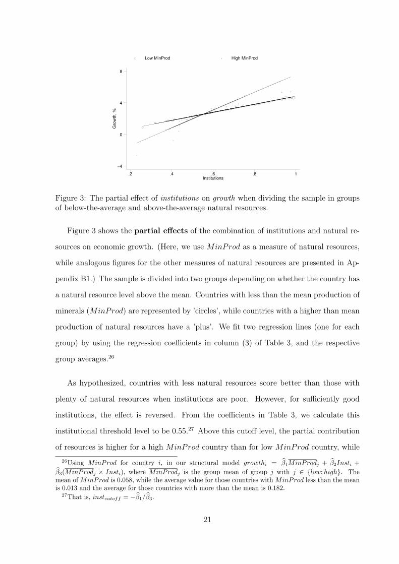
Figure 3: The partial effect of institutions on growth when dividing the sample in groupsof below-the-average and above-the-average natural resources.

Figure 3 shows the partial effects of the combination of institutions and natural re-

sources on economic growth. (Here, we use MinProd as a measure of natural resources,

while analogous figures for the other measures of natural resources are presented in Ap-

pendix B1.) The sample is divided into two groups depending on whether the country has

a natural resource level above the mean. Countries with less than the mean production of

minerals (MinProd) are represented by ’circles’, while countries with a higher than mean

production of natural resources have a ’plus’. We fit two regression lines (one for each

group) by using the regression coefficients in column (3) of Table 3, and the respective

group averages.26

As hypothesized, countries with less natural resources score better than those with

plenty of natural resources when institutions are poor. However, for sufficiently good

institutions, the effect is reversed. From the coefficients in Table 3, we calculate this

institutional threshold level to be 0.55.27 Above this cutoff level, the partial contribution

of resources is higher for a high MinProd country than for low MinProd country, while

26Using MinProd for country i, in our structural model growthi = β1MinProdj + β2Insti +

β3(MinProdj × Insti), where MinProdj is the group mean of group j with j ∈ {low;high}. Themean of MinProd is 0.058, while the average value for those countries with MinProd less than the meanis 0.013 and the average for those countries with more than the mean is 0.182.

27That is, instcutoff = −β1/β3.

21

the opposite holds below the institutional cutoff. In other words, countries with more

resources need relatively better institutions to have the same growth effect as countries

with fewer resources. Moreover, giving further support to our technical appropriability

hypothesis, the institutional threshold level increases somewhat in the technical appropri-

ability of the resource. More specifically, for OrMetExp the institutional cutoff is 0.51,

for MinProd 0.55, and for MidasProd 0.57.

5 Robustness of the results

This section aims at checking the robustness of our results. In the previous section, we

had a wide sample of countries, including both industrialized and developing countries.

We now restrict the sample in various ways. First, we focus on developing countries only,

and find that the results do not depend on the inclusion of rich countries. Furthermore, we

show that dropping potential outliers does not remove our results. Another part of this

section addresses the concern that our results would be driven by a specific continent.

Africa is often mentioned as the continent with the resource curse problem, so that it

might be suspected that excluding Africa would alter our results. While the results turn

out to be somewhat less pronounced, they are still present, however. Excluding Latin

America has a minor effect on the main results.

The subsequent section tackles how measures of conflict affect our main results. The

reason is simply that countries at war ceteris paribus have a lower economic output and

if natural resources fuel conflicts, the importance of the appropriability effect in our main

results may be driven by the existence of conflicts in these countries. This effect turns

out to be without importance for our results, however. Finally we investigate whether the

institutional measure used influences the outcome. Although our main results are qualita-

tively robust to different institutional measures, these regressions reveal some interesting

quantitative effects. In addition, Table 2 reported a high correlation between institutions

and initial GDP level and investments. To check to what extent these correlations influ-

22

ence our conclusions, we used a more parsimonious empirical specification dropping and

adding control variables. These results are presented in Appendix Table B4 for the use

of MidasProd.28

5.1 Excluding the developed countries

Although it is reassuring that our hypothesis has empirical support in a large sample

of countries, much of the resource curse debate has concerned the lack of development

in resource-intensive developing countries in the last decades. Do our hypotheses hold

when restricting the sample to only contain developing countries? This would seem quite

challenging for our results since, by dropping rich countries, we exclude many countries

with high institutional quality, some of which are rich in natural resources and which may

be driving the ”positive” side of the interaction effect. Columns (1)-(4) in Table 6 report

the results when excluding all the countries that where members of the OECD in 1975.29

We find support for a non-monotonic relation between natural resources and growth,

even when considering the developing countries separately. Good institutions are still

crucial when having plenty of highly technically appropriable resources. If anything,

institutional quality in itself appears to be somewhat more important for growth in devel-

oping countries. (For example, comparing the coefficients in column (4) in Table 6 with

the corresponding column in Table 3, gives at hand that the coefficient for institutions

is slightly larger in the sample with only developing countries, while the resources and

the interaction term coefficients are slightly smaller.)

28One specification also includes schooling (see footnote 21). The use of other measures of naturalresources yields the same changes. Moreover, following Sachs and Warner (2001), to address the issue ofreverse causality we have included growth of GDP per capita in the previous period (in our case 1960-1974). Including lagged GDP growth does not alter our main results in any significant respect. Theseresults are available from the authors upon request.

29The excluded countries are Australia, Austria, Belgium, Canada, Denmark, Finland, France, Ger-many, Greece, Iceland, Ireland, Italy, Japan, Luxembourg, Netherlands, New Zealand, Norway, Portugal,Spain, Sweden, United Kingdom, and USA.

23

5.2 Are Botswana and Sierra Leone driving the results?

Naturally, there are countries in our sample differing considerably from all the rest. Just

when eye-balling the data there are certain countries that are outliers either with respect to

their growth performance over the period or their initial endowment of natural resources.

Considering Figures 4(a) and 4(b), obvious outliers in these respects for the MidasProd

measure of natural resources are Botswana and Sierra Leone, for example.30

In

stitu

tio

ns

MidasProd0 .1 .2

.2

.4

.6

.8

1

ARG

AUSAUTBEL

BGD

BOL

BRA

BWA

CANCHE

CHL

CMR

COG

COL

CRI

CYP

DNK

DOMDZA

ECU

EGY

ESP

FIN

FRAGBRGER

GHA

GMB

GRC

GTMGUY

HKG

HND

HTI

IDN

IND

IRL

IRN

ISL

ISR

ITA

JAMJOR

JPN

KEN

KOR

LKA

MEX

MLI

MWI

MYS

NERNIC

NLDNORNZL

PAK

PAN

PER

PHL

PRT

PRYSEN

SGP

SLESLV

SWE

SYRTGO

THA

TTO

TUN

TUR

UGA

URY

USA

VEN

ZAF

ZAR

ZMB

(a) Full Sample

In

stitu

tio

ns

MidasProd, no zeroes, no extremes0 .002 .004 .006 .008

.2

.4

.6

.8

1

ARG

AUSAUT

BOL

BRA

CAN

CHL

CMR

COG

COL

CRI

DZA

ECU

ESP

FIN

FRAGER

GRC

GTMGUY

HND

HTI

IDN

IND

IRL

ITA

JPN

KEN

KOR

MEX

MLI

MYS

NIC

NZL

PER

PHL

PRT

SLV

SWE

TUN

USA

VEN

ZMB

(b) No Extremes

Figure 4: MidasProd and institutions

To check for influential observations, i.e. observations with either a high leverage or

a large residual, we use the DFITS index when estimating equation (3.1). Observations

with a DFITS index larger than the absolute value of 2√

k/n (where k is the number

of independent variables, including the constant, and n the number of observations),

are excluded from the sample.31 Thereby, we obtain a specific sample for each measure

of natural resource endowment. Columns (5)-(8) in Table 6 report the results and the

countries excluded from the sample with each measure of natural resources. The outcome

varies to a surprisingly small extent when excluding outliers. The qualitative results are

in general the same, but the coefficients for natural resources measured as MidasProd

30As seen from Figure 4(a), MidasProd may be problematic in two ways. It has some clear outliersand many countries in the sample simply do not have any production of diamonds or precious metals.Besides our exclusion of influential observations using DFITS, we also ran regressions on MidasProdwhile excluding extreme observations. Excluding countries with zero production has little effect. Whenalso dropping all observations with at least as high a MidasProd as that of the Dominican Republic(leaving us with a sample of 43 countries), the interaction term turns insignificant (p-value 0.14), thoughthe three variables of interest are still jointly significant at the 99 per cent level. These estimates areavailable from the authors upon request.

31DFITSi = ri

√hi/(1 − hi), where ri are the studentised residuals and hi the leverage.

24

turn individually insignificant. However, they are still highly jointly significant, so the

appropriability effect is in line with the basic results.

5.3 Is Africa (or Latin America) responsible for our results?

While the previous section showed that the hypothesis in this paper provides a good

explanation for the developing countries as a group, it might be that the results are

entirely driven by particular regions. Africa is known as a continent with abundant

resources, in particular precious metals, but also for its wars and low income per capita

levels. It is thus a concern that our main results (presented in Table 3) could be driven

by the development of the African continent. In Table 7, columns (1)-(4), we re-estimate

equation (3.1), but drop Africa from the sample. The results clearly indicate that in the

presence of highly appropriable resources (especially MidasProd), good institutions are

quintessential for economic development also when excluding Africa.

Columns (5)-(8) in Table 7 show the same to be true when excluding Latin America.

This is particularly reassuring since recent studies have pointed at the importance of

initial factor endowments and other geographical factors for the shaping of institutions in

Latin America. For example, Sokoloff and Engerman (2000) argue that the casual relation

runs from the initial resource endowment fostering a certain institutional setting, which

can or cannot be beneficial for long-run economic development. Sugar, coffee and cocoa

economies in Latin America are often used to illustrate the point, but also mineral rich

economies such as Chile and Peru. The idea is that the production of these resources

is both valuable and easy to control for a small elite. This elite has all the incentives

to ensure that the ownership of land remains concentrated in its hands, which is most

easily achieved by impeding the spread of education and democratic institutions. Thereby,

initial resource endowment is suggested to generate a strong path dependence affecting

the pattern of economic development. That is, in the setting of this paper, it could be

suspected that natural resources have determined the institutional formation in these

25

countries. Columns (5)-(8) in Table 7 indicate that our main results are not driven by

the presence of Latin American countries.

5.4 Importance of civil wars

A potentially important mechanism, already mentioned in the Introduction, through

which natural resources could affect economic development is by creating conflicts. Allu-

vial diamonds are maybe the resource most known for generating conflicts, but also oil (as

in Sudan) can apparently fuel conflicts. We test whether conflicts affect the importance

of appropriability for economic development by including two different measures. The

first measure, conflict, is a dummy for the occurrence of any kind of conflict during the

period. The country in question can thus be involved in a international or internal war, or

be having a conflict with a neighbouring country. Civil war instead assumes the value of

one if there were a civil war with at least a thousand battle-related deaths in the period.

Neither the inclusion of conflict nor of civil war has a significant effect on the results, as

reported in Table 8; if anything, the appropriability effect of resources becomes slightly

more important. Now, this does not show anything but that our main results are not

driven by conflicts.

5.5 Robustness to other institutional measures

The last robustness check consists of using alternative measures of institutional quality.

Even though institutional measures in general tend to be highly correlated, we test if

our basic equation (3.1) holds with a variety of institutional measures. More specifically,

we use seven measures ranging from Polity75 from the Polity IV data set (Marshall and

Jaggers, 2002) to Rule of Law in 1998 (RLaw98) from Kaufmann et al. (2002). To reduce

the number of tables, we only report the outcomes when using MidasProd as the measure

of initial natural resource endowment. In addition, to increase the comparability of the

estimates, we have rescaled the institutional indexes so as all of them range between 0

26

and 1.

Table 9 reports the regression results. The interaction effect of MidasProd and

institutions is always positive, as expected, and significant. This means that our results

do not appear to be sensitive to the chosen measure of institutional quality. However,

the magnitude of the appropriability effect is approximately five times larger when using

Repud84 instead of Polity75, given the same level of natural resources (Institutions has

a quantitatively intermediate appropriability effect). These results are suggestive of the

mechanisms driving the appropriability of a resource. Copper, oil, kimberlitic diamonds

and other investment intensive and very valuable resources are extremely sensitive to

the investment climate in the host country. Nothing can hurt investments as much as a

regime repudiating contracts, since this radically increases the riskiness of heavy invest-

ments. The extent of democratic rule, as captured by Polity75, on the other hand seems

less important for investment decisions as long as the companies are on friendly terms

with the regime.

6 Summary and concluding remarks

Kenneth Kaunda, the former President of Zambia, has been quoted to say ”We are in part

to blame, but this is the curse of being born with a copper spoon in our mouths”, referring

to Zambia’s poor economic performance.32 In another quote referring to the deterministic,

negative effects of having abundant resources, Leonardo Simao (Minister of Foreign Affairs

of Mozambique) has said, ”Mozambique is different [from Angola]. We are fortunate not

to have oil and not to have diamonds”.33 This paper suggests that such statements need

some modification. The problem for Zambia, and many other countries, does not lie in the

resource richness per se, but in the combination of having poor institutions and resource

wealth. Our results indicate that a sufficient improvement in institutional quality turns

32Ross (1999).33Speech delivered at the Swedish Institute of International Affairs, Stockholm, Sweden on June 18,

1999.

27

resource abundance into an asset rather than a curse.

Furthermore, we have shown the type of natural resources a country possesses to be

of crucial importance. The negative effects of poor institutional quality are much more

severe in countries rich in potentially problematic types of resources, as compared to

those rich in other natural resources. Conversely, the rewards for good institutions are

greatest for the countries with more appropriable types of resources. For all our measures

of mineral-intensity, the positive interaction term outweighs the negative effect of the

resources themselves, and this effect is highly significant. We find the strongest and most

significant effects when using the value of production of precious metals and diamonds.

What are the quantitative implications of our findings? Taking the point estimates

seriously, our results suggest that if a country, such as Sierra Leone (with an average

growth rate of -2.05 per cent since 1975) were to manage to close the gap in institutional

quality with a country like Botswana (with a growth rate of 4.99 per cent over the period),

then its yearly growth rate would also approach that of Botswana. Thus, Sierra Leone has

the potential of performing like Botswana, but it lacks the necessary institutional setting.

This paper challenges the traditional resource curse which, taken literally, would sim-

ply suggest that a country would be better off without its resources. We find this hard to

believe. Identifying a non-montone relationship between institutions and resources, and

the particular role of certain types of minerals, we show that it is possible to reverse the

curse. The literal policy advice of this paper would thus be to ”Get your institutions

right, especially if you have plenty of diamonds and precious metals”. Naturally, this is

not very informative in terms of implementation, but it does suggest that countries can

do something more to improve their economic situation than giving away their resources

– as suggested by the resource curse hypothesis.

28

References

Daron Acemoglu, Simon Johnson, and James A. Robinson. The Colonial Origins ofComparative Development: An Empirical Investigation. American Economic Review,91(5):1396–1401, 2001.

Daron Acemoglu, Simon Johnson, and James A. Robinson. Reversal of Fortune: Geog-raphy and Institutions in the Making of the Modern World Income Distribution. TheQuarterly Journal of Economics, 117(4):1231–1294, November 2002.

Francisco Alcala and Antonio Ciccone. Trade and productivity. Quarterly Journal ofEconomics, 119(2):613–646, 2004.

Richard M. Auty. Sustaining Development in Mineral Economies: The Resource CurseThesis. Routledge, London and New York, 1993.

Richard M. Auty. Natural resource endowment, the state and development strategy.Journal of International Development, 9(4):651–663, 1997.

Robert J. Barro and Jong-Wha Lee. International Data on Educational Attainment,Updates and Implications. Manuscript, Harvard University, August 2000.

Greg Campbell. Blood Diamonds: Tracing the Deadly Path of the World’s Most PreciousStones. Westview Press, Boulder, 2002.

Paul Collier and Anke Hoeffler. Greed and grievance in civil war. Centre for the Study ofAfrican Economies Working Paper, (01), 2002a.

Paul Collier and Anke Hoeffler. On the incidence of civil war. Journal of Conflict Reso-lution, 46:13–28, 2002b.

Paul Collier and Anke Hoeffler. On economic causes of civil war. Oxford Economic Papers,50:563–573, 1998.

W. Max Corden and J. Peter Neary. Booming sector and de-industrialisation in a smallopen economy. Economic Journal, 92:825–848, 1982.

William Easterly and Ross Levine. Tropics, germs and crops: How endowments influenceeconomic development. NBER Working Paper 9106, 2002.

Stanley L. Engerman and Kenneth L. Sokoloff. Factor endowments, inequality, and thepath of development among the new world economies. Work in Progress, 2002.

Alan H. Gelb. Windfall Gains: Blessing or Curse? Oxford University Press, New York,1988.

Thorvaldur Gylfason, Tryggvi T. Herbertson, and Gylfi Zoega. A mixed blessing: Naturalresources and economic growth. Macroeconomic Dynamics, 3:204–225, 1999.

Robert E. Hall and Charles I. Jones. Why Do Some Countries Produce so Much MoreOutput per Worker than Others? The Quarterly Journal of Economics, 114(1):83–116,February 1999.

29

Jonathan Isham, Michael Woolcook, Lant Pritchett, and Gwen Busby. The varieties ofresource experience: How natural resource export structures affect the political economyof economic growth. Middlebury College Discussion Paper 03-08, 2003.

Terry Lynn Karl. The Paradox of Plenty: Oil Booms and Petro-States. University ofCalifornia Press, Berkeley, 1997.

Daniel Kaufmann, Aart Kraay, and Pablo Zoido-Lobaton. Governance matters II – up-dated indicators 2000/01. World Bank Policy Research Working Paper 2772, 2002.

Philip Keefer and Stephen Knack. Polarization, Politics, and Property Rights: Linksbetween inequality and growth. Public Choice, 111:127–154, 2002.

Stephen Knack and Philip Keefer. Institutions and Economic Performance: Cross-Country Tests Using Alternative Institutional Measures. Economic and Politics, 7(3):207–227, 1995.

Paul Krugman. The narrow moving band, the Dutch disease, and the competitive conse-quences of Mrs. Thatcher: Notes on trade in the presence of dynamic scale economies.Journal of Development Economics, 27(1-2):41–55, October 1987.

Rafael La Porta, Florencio Lopez de Silanes, Andrei Shleifer, and Robert W. Vishny. Thequality of government. Manuscript, Harvard University, August, 1998.

Philip R. Lane and Aaron Tornell. The voracity effect. American Economic Review, 89(1):22–46, 1999.

Carlos Leite and Jens Weidmann. Does mother nature corrupt? natural resources, cor-ruption, and economic growth. International Monetary Fund Working Paper 99/85,1999.

Monty G. Marshall and Keith Jaggers. Polity IV Project. Political Regime Characteristicsand Transitions, 1800-2002. Integrated Network for Social Conflict Research (INSCR)Program. Center for International Development and Conflict Management. Universityof Maryland, 2002. Available at www.cidcm.umd.edu/inscr/polity.

Kiminori Matsuyama. Agricultural productivity, comparative advantage and economicgrowth. Journal of Economic Theory, 58:317–334, 1992.

Halvor Mehlum, Karl Moene, and Ragnar Torvik. Institutions and the resource curse.Mimeo, 2002.

Minerals Yearbook. U.S. Bureau of Mines (department of the interior). Washington, DC.U. S. Government printing office. (Various years).

J. Peter Neary and Sweder J. G. van Wijnbergen. Natural Resources and the Macroecon-omy. MIT Press, Cambridge, Mass, 1986.

Oxford History of the British Empire. The Nineteenth Century. Oxford University Press,Oxford, 2001. Ed. Roger Luis.

30

James A. Robinson, Ragnar Torvik, and Thierry Verdier. Political foundations of theresource curse. CEPR Discussion paper 3422, 2002.

Dani Rodrik. Where did all the Growth go? External Shocks, Social Conflict, and GrowthCollapses. Journal of Economic Growth, 4:385–412, 1999.

Dani Rodrik, Arvind Subramanian, and Francesco Trebbi. Institutions rule: The pri-macy of institutions over geography and integration in economic development. CEPRDiscussion Paper 3643, 2002.

Michael L. Ross. Does oil hinder democracy? World Politics, 53(3):325–361, 2001.

Michael L. Ross. The political economy of the resource curse. World Politics, 51(2):297–322, 1999.

Jeffrey D. Sachs and Andrew M. Warner. The curse of natural resources. EuropeanEconomic Review, 45(4-6):827–838, 2001.

Jeffrey D. Sachs and Andrew M. Warner. Natural resource abundance and economicgrowth. NBER Working Paper 5398, 1995.

Jeffrey D. Sachs and Andrew M. Warner. Sources of slow growth in African economies.Journal of African Economies, 6:335–376, 1997.

Kenneth L. Sokoloff and Stanley L. Engerman. History lessons: Institutions, factor endow-ments, and paths of development in the new world. Journal of Economic Perspectives,14(3):217–232, 2000.

Havard Strand, Lars Wilhelmsen, and Nils Petter Gleditsch. Armed Conflict DatasetCodebook, Version 1.1. International Peace Research Institute, Oslo, 2002.

Ragnar Torvik. Natural resources, rent seeking and welfare. Journal of DevelopmentEconomics, 67:455–470, 2002.

UNCTAD. Handbook of international trade and development statistics. United Nations.(Various years).

U.S. Geological Survey. (Department of the Interior). Metal Prices in the United Statesthrough 1998. Washington, DC. U. S. Government printing office, 1999. (available athttp://minerals.usgs.gov).

Michael Woolcook, Lant Pritchett, and Jonathan Isham. The social foundations of pooreconomic growth in resource rich economies. In Richard M. Auty, editor, ResourceAbundance and Economic Development, New York, 2001. Oxford University Press.

Gavin Wright. Resource-based growth then and now. Stanford University. (Prepared forthe World Bank Project ”Patterns of Integration in the Global Economy”), 2001.

31

Tables

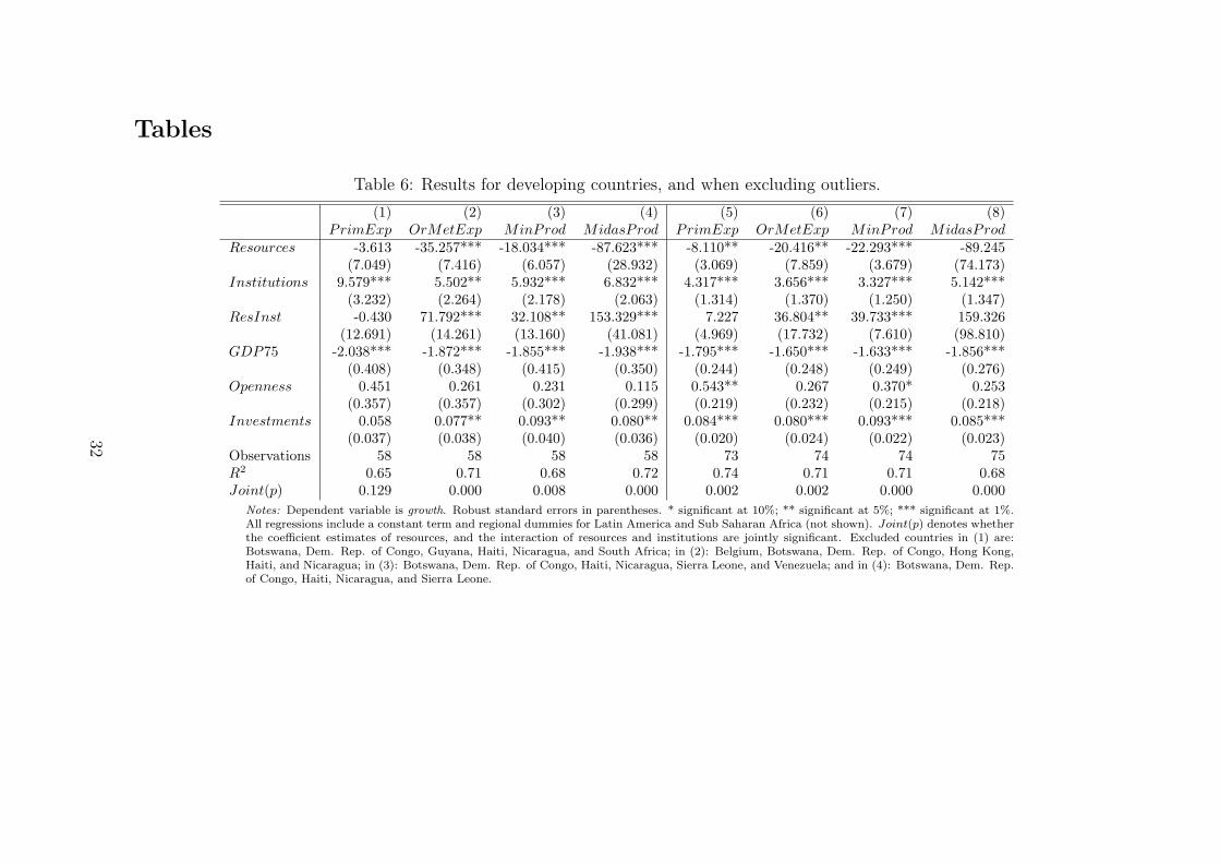
Table 6: Results for developing countries, and when excluding outliers.

(1) (2) (3) (4) (5) (6) (7) (8)PrimExp OrMetExp MinProd MidasProd PrimExp OrMetExp MinProd MidasProd

Resources -3.613 -35.257*** -18.034*** -87.623*** -8.110** -20.416** -22.293*** -89.245(7.049) (7.416) (6.057) (28.932) (3.069) (7.859) (3.679) (74.173)

Institutions 9.579*** 5.502** 5.932*** 6.832*** 4.317*** 3.656*** 3.327*** 5.142***(3.232) (2.264) (2.178) (2.063) (1.314) (1.370) (1.250) (1.347)

ResInst -0.430 71.792*** 32.108** 153.329*** 7.227 36.804** 39.733*** 159.326(12.691) (14.261) (13.160) (41.081) (4.969) (17.732) (7.610) (98.810)

GDP75 -2.038*** -1.872*** -1.855*** -1.938*** -1.795*** -1.650*** -1.633*** -1.856***(0.408) (0.348) (0.415) (0.350) (0.244) (0.248) (0.249) (0.276)

Openness 0.451 0.261 0.231 0.115 0.543** 0.267 0.370* 0.253(0.357) (0.357) (0.302) (0.299) (0.219) (0.232) (0.215) (0.218)

Investments 0.058 0.077** 0.093** 0.080** 0.084*** 0.080*** 0.093*** 0.085***(0.037) (0.038) (0.040) (0.036) (0.020) (0.024) (0.022) (0.023)

Observations 58 58 58 58 73 74 74 75R2 0.65 0.71 0.68 0.72 0.74 0.71 0.71 0.68Joint(p) 0.129 0.000 0.008 0.000 0.002 0.002 0.000 0.000

Notes: Dependent variable is growth. Robust standard errors in parentheses. * significant at 10%; ** significant at 5%; *** significant at 1%.All regressions include a constant term and regional dummies for Latin America and Sub Saharan Africa (not shown). Joint(p) denotes whetherthe coefficient estimates of resources, and the interaction of resources and institutions are jointly significant. Excluded countries in (1) are:Botswana, Dem. Rep. of Congo, Guyana, Haiti, Nicaragua, and South Africa; in (2): Belgium, Botswana, Dem. Rep. of Congo, Hong Kong,Haiti, and Nicaragua; in (3): Botswana, Dem. Rep. of Congo, Haiti, Nicaragua, Sierra Leone, and Venezuela; and in (4): Botswana, Dem. Rep.of Congo, Haiti, Nicaragua, and Sierra Leone.

32

Table 7: Results when excluding Sub Saharan Africa or Latin America.

(1) (2) (3) (4) (5) (6) (7) (8)PrimExp OrMetExp MinProd MidasProd PrimExp OrMetExp MinProd MidasProd

Resources -6.551 -6.906 -14.186** -403.961** -6.325 -27.107** -21.568*** -87.306***(5.064) (6.760) (6.563) (177.626) (4.926) (10.803) (4.023) (29.269)

Institutions 5.366*** 5.587*** 5.082*** 5.540*** 7.241*** 5.368*** 4.833*** 5.608***(1.550) (1.501) (1.481) (1.361) (2.313) (1.879) (1.399) (1.351)

ResInst 4.427 12.562 23.048** 629.596* 4.794 49.217** 41.682*** 154.989***(6.709) (14.857) (11.280) (354.121) (6.946) (24.097) (7.486) (40.608)

GDP75 -2.067*** -2.079*** -2.034*** -2.101*** -2.286*** -2.098*** -1.975*** -2.008***(0.317) (0.324) (0.341) (0.324) (0.437) (0.364) (0.283) (0.258)

Openness 0.515* 0.236 0.303 0.301 0.598** 0.419 0.473* 0.366(0.259) (0.311) (0.266) (0.254) (0.285) (0.332) (0.269) (0.273)

Investments 0.084*** 0.090*** 0.093*** 0.093*** 0.092*** 0.095*** 0.107*** 0.090***(0.025) (0.027) (0.026) (0.025) (0.026) (0.028) (0.026) (0.024)

Observations 64 64 64 64 58 58 58 58R2 0.60 0.58 0.59 0.60 0.71 0.74 0.78 0.81Joint(p) 0.102 0.587 0.106 0.068 0.160 0.001 0.000 0.000

Notes: Dependent variable is growth. Robust standard errors in parentheses. * significant at 10%; ** significant at 5%; *** significant at1%. All regressions include a constant term and regional dummies for Latin America and Sub Saharan Africa (not shown). Joint(p) denoteswhether the coefficient estimates of resources, and the interaction of resources and institutions, are jointly significant.

33

Table 8: Results when including measures of conflicts.

(1) (2) (3) (4) (5) (6) (7) (8)PrimExp OrMetExp MinProd MidasProd PrimExp OrMetExp MinProd MidasProd

Resources -6.919 -26.720*** -21.856*** -95.803*** -6.316 -27.982*** -19.363*** -89.229***(4.624) (8.416) (5.072) (28.239) (4.108) (8.707) (4.808) (30.521)

Institutions 6.390*** 4.388** 3.736** 5.520*** 5.847*** 3.374** 4.115*** 4.952***(2.191) (1.806) (1.518) (1.489) (2.045) (1.589) (1.406) (1.428)

ResInst 5.001 51.067*** 39.765*** 167.403*** 4.201 52.958*** 35.102*** 158.615***(6.807) (18.011) (9.641) (38.984) (6.141) (19.045) (9.143) (41.933)

GDP75 -2.167*** -1.975*** -1.837*** -2.013*** -2.124*** -1.903*** -1.909*** -1.968***(0.389) (0.344) (0.311) (0.304) (0.360) (0.289) (0.290) (0.270)

Openness 0.483* 0.203 0.222 0.138 0.426 0.150 0.228 0.092(0.267) (0.293) (0.242) (0.246) (0.291) (0.308) (0.272) (0.265)

Investments 0.085*** 0.088*** 0.098*** 0.088*** 0.086*** 0.090*** 0.102*** 0.088***(0.026) (0.029) (0.026) (0.026) (0.025) (0.027) (0.026) (0.026)

Conflict -0.166 -0.267 -0.434 -0.028(0.402) (0.385) (0.395) (0.359)

Civil War -0.569 -0.826 -0.380 -0.443(0.501) (0.506) (0.511) (0.531)

Observations 80 80 80 80 80 80 80 80R2 0.63 0.65 0.67 0.70 0.64 0.67 0.67 0.71Joint(p) 0.053 0.005 0.000 0.000 0.056 0.002 0.001 0.000

Notes: Dependent variable is growth. Robust standard errors in parentheses. * significant at 10%; ** significant at 5%; *** significant at 1%.All regressions include a constant term and regional dummies for Latin America and Sub Saharan Africa (not shown). Joint(p) denotes whetherthe coefficient estimates of resources, and the interaction of resources and institutions, are jointly significant.

34

Table 9: Results when using alternative institutional measures

(1) (2) (3) (4) (5) (6)Polity75 PropRight84 RLaw84 Exprop84 Repud84 KKZ98

MidasProd -53.676* -102.199*** -69.226 -154.248*** -154.841*** -58.965***(27.213) (32.204) (48.935) (32.485) (57.234) (17.719)

AltInst 0.512 4.274*** 2.121* 3.648*** 4.279*** 3.550***(0.564) (1.191) (1.082) (1.021) (1.096) (1.076)

ResInst 81.498*** 184.947*** 108.694* 253.365*** 292.938*** 128.846***(29.339) (48.624) (58.775) (45.963) (95.151) (27.085)

GDP75 -1.140*** -1.960*** -1.426*** -1.543*** -1.800*** -1.497***(0.238) (0.304) (0.356) (0.222) (0.252) (0.264)

Openness 0.019 0.142 0.192 0.129 0.049 -0.016(0.231) (0.248) (0.229) (0.240) (0.268) (0.234)

Investments 0.118*** 0.092*** 0.095*** 0.086*** 0.111*** 0.098***(0.027) (0.025) (0.025) (0.024) (0.023) (0.023)

Observations 78 76 76 76 76 80R2 0.63 0.69 0.62 0.69 0.68 0.69Joint(p) 0.000 0.000 0.000 0.000 0.000 0.000

Notes: Dependent variable is growth. Robust standard errors in parentheses. * significant at 10%; ** significantat 5%; *** significant at 1%. All regressions include a constant term and regional dummies for Latin Americaand Sub Saharan Africa (not shown). Joint(p) denotes whether the coefficient estimates of resources, and theinteraction of resources and institutions are jointly significant.

35

Appendix A. Sources and summary statistics

Table A1: Countries in the sample

Algeria JamaicaArgentina JapanAustralia JordanAustria KenyaBangladesh Korea, Republic ofBelgium MalawiBolivia MalaysiaBotswana MaliBrazil MexicoCameroon NetherlandsCanada New ZealandChile NicaraguaColombia NigerCongo, Democratic Republic* NorwayCongo, Republic of PakistanCosta Rica PanamaCyprus* ParaguayDenmark PeruDominican Republic PhilippinesEcuador PortugalEgypt SenegalEl Salvador Sierra Leone*Finland Singapore*France South AfricaGambia, The SpainGermany Sri LankaGhana SwedenGreece SwitzerlandGuatemala SyriaGuyana ThailandHaiti TogoHonduras Trinidad and TobagoHong Kong TunisiaIceland TurkeyIndia USAIndonesia UgandaIran United KingdomIreland UruguayIsrael VenezuelaItaly Zambia* These countries are, due to data availability, measured until 1996.

36

Table A2: Definitions and sources of variables

PrimExp Share of exports of primary products in GNP in 1971. Source: Sachsand Warner (1995), where it is labelled SXP.

OrMetExp Value of export of ores and metals as a share of GDP in 1975. Source:UNCTAD (1975, 1979)

MinProd Share of mineral production (does not include fuels) in GNP in 1971,where ”mineral production” is the production value of the 23 highestvalued minerals in the world as of 1973. Source: Sachs and Warner(1995) where it is labelled SNR.

MidasProd Value of the production of gold, silver, platinum group metals and di-amonds as a share of GDP, average 1972 to 1980. Source: Own cal-culations from Minerals Yearbook (various years), and U.S. GeologicalSurvey (1999).

Institutions Derived from the IRIS data originally constructed by Knack and Keefer(1995) based on data from the International Country Risk Guide. Thefive Property Right Index components are Quality of the bureaucracy,Corruption in government, and Rule of law, scoring from 0-6, and Riskof expropriation of private investment, and Repudiation of contractsby government, scored 0-10. Higher scores mean better quality, lowercorruption and lower risks. By transforming the first three into tenpoint scales (as do Keefer and Knack, 2002), the (unweighted) sum givesan index from 0 to 50 which we rescale into an index between zero andone. Source: Keefer and Knack (2002)).

Growth Average yearly growth rate (in per cent) between 1975 and 1998. Calcu-lated as ln(rgdpch98)-ln(rgdpch75)* 100/20, where rgdpch is the PPP-adjusted GDP per capita between 1975 and 1998. Source: Penn WorldTable, Mark 6.1.

GDP75 Real GDP per capita in constant dollars (Chain index) expressed ininternational prices ln(rgdpch75). Source: Penn World Table, Mark 6.1

Schooling Average schooling years in the total population 1975. Source: Barro andLee (2000).

Openness Natural logarithm of average openness (openc) 1975 to 1998. Source:Penn World Table, Mark 6.1.

Investments Average investment share of real GDP per capita (ki) 1975 to 1998.Source: Penn World Table, Mark 6.1.

Latitude The absolute value of the latitude of the country, scaled to take valuesbetween 0 and 1. Source: La Porta et al. (1998).

Conflict Dummy for occurrence of conflict during period. It refers to any type ofconflict with at least 25 battle-related deaths per year during the conflict.Source: Strand et al. (2002).

Civil war Dummy for any civil war started during the period leading to at least1000 battle-related deaths. Source: Collier and Hoeffler (2002b).

37

Table A3: Summary statistics, entire sampleVariable Mean S.D. Min Max

Growth 1.533 1.965 -5.391 5.968PrimExp 0.121 0.101 0.006 0.543OrMetExp 0.041 0.068 0 0.357MinProd 0.058 0.097 0 0.509MidasProd 0.006 0.025 0 0.198Institutions 0.638 0.215 0.232 0.995GDP75 8.332 0.98 6.389 9.923Openness 4.045 0.55 2.79 5.899Investments 16.875 7.701 2.38 44.231

N 80

Table A4: Summary statistics, developing countriesVariable Mean S.D. Min Max

Growth 1.341 2.241 -5.391 5.968PrimExp 0.137 0.107 0.01 0.543OrMetExp 0.046 0.078 0 0.357MinProd 0.074 0.109 0 0.509MidasProd 0.008 0.029 0 0.198Institutions 0.53 0.135 0.232 0.872GDP75 7.881 0.749 6.389 9.306Openness 4.054 0.584 2.79 5.899Investments 14.478 7.538 2.38 44.231

N 58

Table A5: Summary statistics, other institutional measuresVariable Mean S.D. Min. Max. N

polity75 0.532 0.399 0 1 78propright84 0.574 0.25 0.189 0.992 76rule84 0.539 0.298 0.167 1 76expropriati84 0.614 0.215 0.18 0.98 76repudate84 0.601 0.209 0.16 0.98 76rlaw98 0.574 0.244 0 1 80

38

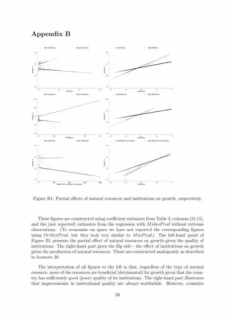
Appendix BG

row

th,

%

MinProd

’Bad’ institutions ’Good’ institutions

0 .2 .4 .6

−4

0

4

8

Gro

wth

, %

Institutions

Low MinProd High MinProd

.2 .4 .6 .8 1

−4

0

4

8

Gro

wth

, %

MidasProd

’Bad’ institutions ’Good’ institutions

0 .05 .1 .15 .2

−5

0

5

10

15

Gro

wth

, %

Institutions

Low MidasProd High MidasProd

.2 .4 .6 .8 1

−5

0

5

10

Gro

wth

, %

MidasProd (no zeroes, no extremes)

’Bad’ institutions ’Good’ institutions

0 .002 .004 .006 .008

0

2

4

6

Gro

wth

, %

Institutions

Low MidasProd (no zeroes) High MidasProd (no extremes)

.2 .4 .6 .8 1

0

2

4

6

Figure B1: Partial effects of natural resources and institutions on growth, respectively.

These figures are constructed using coefficient estimates from Table 3, columns (3)-(4),and the (not reported) estimates from the regression with MidasProd without extremeobservations. (To economise on space we have not reported the corresponding figuresusing OrMetProd, but they look very similar to MinProd.) The left-hand panel ofFigure B1 presents the partial effect of natural resources on growth given the quality ofinstitutions. The right-hand part gives the flip side - the effect of institutions on growthgiven the production of natural resources. These are constructed analogously as describedin footnote 26.

The interpretation of all figures to the left is that, regardless of the type of naturalresource, more of the resources are beneficial (detrimental) for growth given that the coun-try has sufficiently good (poor) quality of its institutions. The right-hand part illustratesthat improvements in institutional quality are always worthwhile. However, countries

39

with more resources need better institutions to have the same growth effect as countrieswith fewer resources.

Above the institutional threshold level, the partial contribution to growth of resourcesis higher for a country with plenty of resources than for a country with few resources.Below the institutional cutoff, the effect is reversed. Furthermore, considering our techni-cally appropriability hypothesis, the institutional threshold level increases in the technicalappropriability of the resource. More specifically, for OrMetProd the institutional cutoffis 0.51, for MinProd 0.55, for MidasProd 0.57, and for MidasProd excluding extremes,it is 0.82.

40

Table B1: First-stage regressions when instrumenting institutions with latitude and fraction speaking any Europeanlanguage

(1) (2) (3) (4) (5) (6) (7) (8)PrimExp PrimExpX OrMetExp OrMetExpX MinProd MinProdX MidasProd MidasProdX

latitude 0.198** -0.066*** 0.152* -0.014** 0.195** -0.031*** 0.210*** -0.000(0.093) (0.023) (0.086) (0.007) (0.076) (0.011) (0.074) (0.001)

ResLat 0.297 0.789*** 2.433*** 0.979*** -0.574 0.803*** 8.970** 1.747***(0.434) (0.181) (0.864) (0.141) (0.960) (0.256) (4.072) (0.152)

EurFrac 0.094*** 0.004 0.095*** 0.002 0.084*** 0.004 0.091*** 0.000(0.026) (0.006) (0.026) (0.002) (0.024) (0.003) (0.026) (0.000)

Observations 80 80 80 80 80 80 80 80Significance of instruments:F (3, 70) 6.38 8.22 8.18 16.68 4.99 7.94 8.14 76.39p − value 0.001 0.000 0.000 0.000 0.003 0.000 0.000 0.000

Notes: The dependent variable is institutions in odd-numbered columns, and the interaction of institutions and natural resources in even-numberedcolumns. Robust standard errors in parentheses. * significant at 10%; ** significant at 5%; *** significant at 1%. Significance of instruments reportsthe F-test for joint significance of excluded instruments. See Section 4 for details.41

Table B2: First-stage regressions when instrumenting institutions with settler mortality, latitude and fractionspeaking any European language

(1) (2) (3) (4) (5) (6) (7) (8)PrimExp PrimExpX OrMetExp OrMetExpX MinProd MinProdX MidasProd MidasProdX

latitude 0.044 -0.061 -0.035 -0.010 -0.059 -0.036 0.007 -0.002***(0.153) (0.056) (0.088) (0.009) (0.130) (0.023) (0.088) (0.001)

ResLat 0.387 0.675 4.227*** 0.916*** 1.515 0.661 33.650*** 1.828***(1.111) (0.500) (1.006) (0.152) (1.542) (0.446) (6.491) (0.109)

EurFrac 0.121** 0.001 0.133** 0.003 0.125** 0.007 0.114** -0.000(0.056) (0.016) (0.049) (0.005) (0.053) (0.008) (0.053) (0.000)

lsettler -0.061*** 0.001 -0.037* -0.001 -0.028 0.003 -0.038* 0.000(0.020) (0.007) (0.021) (0.001) (0.021) (0.003) (0.022) (0.000)

ResSet 0.191** -0.009 0.170* 0.007 0.093 -0.051* 2.406*** 0.025**(0.072) (0.037) (0.096) (0.009) (0.099) (0.026) (0.598) (0.012)

Observations 50 50 50 50 50 50 50 50Significance of instruments:F 2.62 0.64 5.43 10.62 1.36 4.33 6.44 1822.92p − value 0.039 0.668 0.001 0.000 0.260 0.003 0.000 0.000

Notes: The dependent variable is institutions in odd-numbered columns, and the interaction of institutions and natural resources in even-numberedcolumns. Robust standard errors in parentheses. * significant at 10%; ** significant at 5%; *** significant at 1%. Significance of instruments reportsthe F-test for joint significance of excluded instruments. See Section 4 for details.

42

Table B3: Results when instrumenting for institutions usingsettler mortality.

(1) (2) (3) (4)PrimExp OrMetExp MinProd MidasProd

Res 15.654 -36.407* -12.907 -81.665**(19.030) (20.136) (8.367) (30.608)

Institutions 5.582 0.408 4.067 10.422**(6.461) (6.577) (6.938) (4.846)

ResInst -34.878 74.139* 21.420 151.961***(32.018) (39.997) (17.521) (44.199)

GDP75 -1.155 -1.260 -1.732 -2.758***(1.323) (1.026) (1.312) (0.882)

Openness 0.293 0.233 0.162 0.112(0.365) (0.416) (0.346) (0.392)

Investments 0.083 0.092** 0.094** 0.071(0.063) (0.039) (0.043) (0.047)

Observations 50 50 50 50R2 0.48 0.60 0.65 0.62Joint(p) 0.150 0.185 0.263 0.002Ovid 0.318 0.239 0.200 0.086

First-stage results in Appendix Table B2

Notes: Dependent variable is growth. Robust standard errors in parentheses.* significant at 10%; ** significant at 5%; *** significant at 1%. All regressionsinclude a constant term and regional dummies for Latin America and Sub Sa-haran Africa (not shown). Joint(p) denotes whether the coefficient estimatesof resources, and the interaction of resources and institutions are jointly sig-nificant. Ovid reports the p-values from the Hansen J-overidentification testfor instruments. Hausman reports p-values of the regression-based Hausmantest for endogeneity as explained in the text. The null hypothesis is thatinstitutions are exogenous.

43

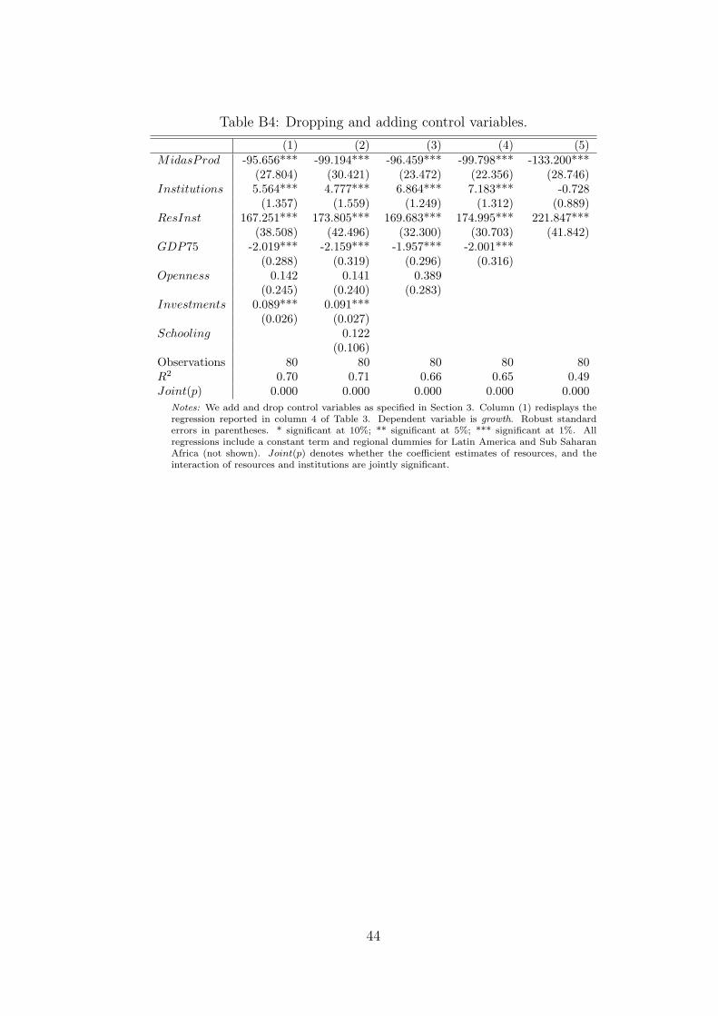
Table B4: Dropping and adding control variables.

(1) (2) (3) (4) (5)MidasProd -95.656*** -99.194*** -96.459*** -99.798*** -133.200***

(27.804) (30.421) (23.472) (22.356) (28.746)Institutions 5.564*** 4.777*** 6.864*** 7.183*** -0.728

(1.357) (1.559) (1.249) (1.312) (0.889)ResInst 167.251*** 173.805*** 169.683*** 174.995*** 221.847***

(38.508) (42.496) (32.300) (30.703) (41.842)GDP75 -2.019*** -2.159*** -1.957*** -2.001***

(0.288) (0.319) (0.296) (0.316)Openness 0.142 0.141 0.389

(0.245) (0.240) (0.283)Investments 0.089*** 0.091***

(0.026) (0.027)Schooling 0.122

(0.106)Observations 80 80 80 80 80R2 0.70 0.71 0.66 0.65 0.49Joint(p) 0.000 0.000 0.000 0.000 0.000

Notes: We add and drop control variables as specified in Section 3. Column (1) redisplays theregression reported in column 4 of Table 3. Dependent variable is growth. Robust standarderrors in parentheses. * significant at 10%; ** significant at 5%; *** significant at 1%. Allregressions include a constant term and regional dummies for Latin America and Sub SaharanAfrica (not shown). Joint(p) denotes whether the coefficient estimates of resources, and theinteraction of resources and institutions are jointly significant.

44