resourcemanagement inwireless cellular networks
TRANSCRIPT

Resource Management in Wireless CellularNetworks with Heterogeneous Capacity Supply
and Heterogeneous Traffic Demand (HetHetNets)
by
Ziyang Wang
A thesis submitted to the
Faculty of Graduate and Postdoctoral Affairs
in partial fulfillment of the requirements for the degree of
Master of Applied Science in Electrical and Computer Engineering
Ottawa-Carleton Institute for Electrical and Computer Engineering
Department of Systems and Computer Engineering
Carleton University
Ottawa, Ontario
September, 2014
c©Copyright
Ziyang Wang, 2014

The undersigned hereby recommends to the
Faculty of Graduate and Postdoctoral Affairs
acceptance of the thesis
Resource Management in Wireless Cellular Networks withHeterogeneous Capacity Supply and Heterogeneous Traffic
Demand (HetHetNets)
submitted by Ziyang Wang
in partial fulfillment of the requirements for the degree of
Master of Applied Science in Electrical and Computer Engineering
Professor Halim Yanikomeroglu, Thesis Co-Supervisor
Professor Marc St-Hilaire, Thesis Co-supervisor
Professor Nancy Samaan, Internal Examiner
Professor Roshdy Hafez, ChairDepartment of Systems and Computer Engineering
Ottawa-Carleton Institute for Electrical and Computer Engineering
Department of Systems and Computer Engineering
Carleton University
September, 2014
ii
Abstract
The term HetNets (heterogeneous networks) is used to describe cellular networks
in which the capacity supply is heterogeneous due to the overlaid architecture of
macrocells and small-cells.
In this thesis we use the term HetHetNets to refer to cellular networks in which the
traffic demand is also heterogeneous due to reasons such as user spatial clustering and
diversified user traffic types, in addition to the heterogeneity in the capacity supply.
The main objective of this thesis is to study the essential problem of matching
the traffic demand (“load”) with the capacity supply (“capacity”) in resource-limited
HetHetNets; this problem is expected to be a major concern in the fifth generation
(5G) cellular networks.
This thesis proposes two approaches to address this problem. One approach is
to deploy small-cells to the centers of user clusters (put supply where needed), and
another approach is to guide users to the cells that are lightly loaded (load balancing
via spatial traffic shaping).
We first investigate how to model the spatial non-uniform (i.e., heterogeneous)
user distribution, and then the impact of user spatial heterogeneity on HetNets is
evaluated. Simulation-based analyses show that network performance deteriorates
significantly with the increase in user spatial heterogeneity if the user locations are
uncorrelated with the locations of the macro and small-cell base stations. Cluster
analysis on the non-uniform user points is then utilized to find the cluster centroids
as the potential locations for small-cells. Simulation results show that the network
performance can improve substantially with increasing user spatial heterogeneity if
we deploy small-cells in the appropriate locations.
The second approach is enabled by the recently developed user-in-the-loop (UIL)
paradigm. In the literature, there have been several investigations on load-aware
cell association as an approach to match traffic demand with the capacity supply,
in which a user may associate to a less loaded cell, even though that cell does not
iii

necessarily provide the maximum SINR. In other words, a user is associated with a cell
to get more share of resources at the cost of lower spectral efficiency. While, the UIL
approach can increase the user received SINR and the share of allocated resources at
the same time, which encourages a user to move to a new location that maximizes the
utility function considering received SINR, cell load and the probability of moving.
Numerical results show that the UIL can double the mean user rate in comparison
to the load-aware cell association strategy, and also results in a more balanced load
across the network.
iv

I would like to dedicate my thesis to my wife Wuyi and my son Dale.
v

Acknowledgments
First and foremost, I am extremely grateful to my supervisors Prof. Halim
Yanikomeroglu and Prof. Marc St-Hilaire for their guidance, support, generosity,
motivation and encouragement during the past two years. Without Prof. Marc St-
Hilaire’s recognition, I would not have had the chance to come to Carleton University,
and without Prof. Halim Yanikomeroglu’s appreciation, I would not have had the
chance to be a member of a prestigious research group that I have benefited so much
from.
I am also extremely thankful to Dr. Rainer Schoenen for his consistent guidance
and encouragement. He has spent so much effort on my research, and his broad
knowledge has saved me from losing directions so many times.
Sincere thanks to all my colleagues for their support in both my research and my
personal life, especially to Mehmet Cagri Ilter, Hamza Umit Sokun, Yaser Fouad,
Meisam Mirahan, Irem Bor and Ramy Gohary. This brotherhood has made me
stronger and optimistic when I am under difficulties.
I would also like to thank my friend and mentor Qiangmin Yu for giving me
enlightenment that has changed my life.
On the personal side, I want to thank my family for their unconditional love.
Without their support and faith in me, I would not be the man I am today.
vi

Table of Contents
Abstract iii
Acknowledgments vi
Table of Contents vii
List of Tables x
List of Figures xi
List of Abbreviations xiii
1 Introduction 1
1.1 Definition . . . . . . . . . . . . . . . . . . . . . . . . . . . . . . . . . 1
1.2 Problem Statement and Motivation . . . . . . . . . . . . . . . . . . . 1
1.3 Contributions and Organization . . . . . . . . . . . . . . . . . . . . . 3
2 Model for User Spatial Heterogeneity 6
2.1 Point Processes in Stochastic Geometry . . . . . . . . . . . . . . . . . 6
2.1.1 Poisson Point Process . . . . . . . . . . . . . . . . . . . . . . 7
2.1.2 Binomial Point Process . . . . . . . . . . . . . . . . . . . . . . 7
2.1.3 Hard Core Point Process . . . . . . . . . . . . . . . . . . . . . 8
2.1.4 Poisson Cluster Process . . . . . . . . . . . . . . . . . . . . . 8
2.2 Log Gaussian Cox Process . . . . . . . . . . . . . . . . . . . . . . . . 8
2.3 Measure of User Spatial Heterogeneity . . . . . . . . . . . . . . . . . 12
2.3.1 Related Work . . . . . . . . . . . . . . . . . . . . . . . . . . . 13
2.3.2 Unified and Nonparameterized Metrics . . . . . . . . . . . . . 14
2.4 Summary . . . . . . . . . . . . . . . . . . . . . . . . . . . . . . . . . 16
vii

3 The Impact of User Spatial Heterogeneity 17
3.1 Guidelines of Performance Evaluation . . . . . . . . . . . . . . . . . . 17
3.1.1 Network Layout . . . . . . . . . . . . . . . . . . . . . . . . . . 18
3.1.2 Antenna Characteristics . . . . . . . . . . . . . . . . . . . . . 19
3.1.3 Channel Model . . . . . . . . . . . . . . . . . . . . . . . . . . 21
3.2 Finite User Rate Demand and Resource Allocation Scheme . . . . . . 23
3.3 Performance Evaluation . . . . . . . . . . . . . . . . . . . . . . . . . 27
3.3.1 The Impact of User Spatial Heterogeneity . . . . . . . . . . . 27
3.3.2 The Impact of Finite Rate Demand . . . . . . . . . . . . . . . 29
3.4 Summary . . . . . . . . . . . . . . . . . . . . . . . . . . . . . . . . . 30
4 Pushing Capacity Supply to Traffic Demand 31
4.1 Related Work . . . . . . . . . . . . . . . . . . . . . . . . . . . . . . . 31
4.2 Cluster Analysis . . . . . . . . . . . . . . . . . . . . . . . . . . . . . . 32
4.2.1 Basic k-means Algorithm . . . . . . . . . . . . . . . . . . . . . 32
4.2.2 Preprocessing and Postprocessing . . . . . . . . . . . . . . . . 33
4.2.3 Selection Criteria . . . . . . . . . . . . . . . . . . . . . . . . . 34
4.3 Performance Evaluation . . . . . . . . . . . . . . . . . . . . . . . . . 37
4.3.1 Small-cell Deployment Strategy . . . . . . . . . . . . . . . . . 37
4.3.2 Fairness Index . . . . . . . . . . . . . . . . . . . . . . . . . . . 39
4.4 Summary . . . . . . . . . . . . . . . . . . . . . . . . . . . . . . . . . 41
5 Pushing Traffic Demand to Capacity Supply 42
5.1 Related Work . . . . . . . . . . . . . . . . . . . . . . . . . . . . . . . 43
5.2 System Model for Spatial Traffic Shaping . . . . . . . . . . . . . . . . 44
5.3 User Model . . . . . . . . . . . . . . . . . . . . . . . . . . . . . . . . 46
5.3.1 User Traffic Classes . . . . . . . . . . . . . . . . . . . . . . . . 46
5.3.2 Resource Allocation . . . . . . . . . . . . . . . . . . . . . . . . 47
5.3.3 Probability of Moving: the P function . . . . . . . . . . . . . 48
5.4 Proposed UIL Load Balancing Approach . . . . . . . . . . . . . . . . 50
5.4.1 Utility Function of GBR Users . . . . . . . . . . . . . . . . . . 51
5.4.2 Utility Function of BE Users . . . . . . . . . . . . . . . . . . . 51
5.4.3 Sequential Optimization . . . . . . . . . . . . . . . . . . . . . 52
5.4.4 An Example of Load Balancing Achieved by UIL . . . . . . . 53
5.4.5 Outlook: Include Mobility Model . . . . . . . . . . . . . . . . 54
viii

5.5 Load-Aware Cell Association . . . . . . . . . . . . . . . . . . . . . . . 54
5.5.1 Related Work . . . . . . . . . . . . . . . . . . . . . . . . . . . 56
5.5.2 Proposed Scheme . . . . . . . . . . . . . . . . . . . . . . . . . 57
5.6 Numerical Results . . . . . . . . . . . . . . . . . . . . . . . . . . . . . 58
5.6.1 Simulation Setup . . . . . . . . . . . . . . . . . . . . . . . . . 58
5.6.2 Transient and Steady State Behavior . . . . . . . . . . . . . . 60
5.6.3 Loads among Different Cells . . . . . . . . . . . . . . . . . . . 61
5.6.4 GBR Users Outage . . . . . . . . . . . . . . . . . . . . . . . . 63
5.6.5 Mean User Rate . . . . . . . . . . . . . . . . . . . . . . . . . . 65
5.6.6 Fairness Index . . . . . . . . . . . . . . . . . . . . . . . . . . . 66
5.7 Summary . . . . . . . . . . . . . . . . . . . . . . . . . . . . . . . . . 67
6 Conclusion and Future Work 69
6.1 Conclusion . . . . . . . . . . . . . . . . . . . . . . . . . . . . . . . . . 69
6.2 Future Work . . . . . . . . . . . . . . . . . . . . . . . . . . . . . . . . 71
6.2.1 Pushing Capacity Supply to Traffic Demand . . . . . . . . . . 71
6.2.2 Pushing Traffic Demand to Capacity Supply . . . . . . . . . . 71
List of References 72
ix

List of Tables
2.1 Basic statistics of distance-based measures for a PPP in one, two and
three dimensions. . . . . . . . . . . . . . . . . . . . . . . . . . . . . . 15
3.1 Path loss model . . . . . . . . . . . . . . . . . . . . . . . . . . . . . . 22
3.2 Simulation parameters in Chapter 3 and Chapter 4 . . . . . . . . . . 22
5.1 Simulation parameters in Chapter 5 . . . . . . . . . . . . . . . . . . . 58
x

List of Figures
1.1 An example of HetNets architecture. . . . . . . . . . . . . . . . . . . 2
1.2 Contributions and organization . . . . . . . . . . . . . . . . . . . . . 4
2.1 A realization of a PPP and its corresponding HCPP and PCP. . . . . 9
2.2 An example of the intensity maps of a PPP and a LGCP . . . . . . . 10
2.3 An example of user distribution with different deviation in LGCP. . . 11
2.4 Voronoi and Delaunay tessellations. . . . . . . . . . . . . . . . . . . . 14
3.1 Macrocell geometry. . . . . . . . . . . . . . . . . . . . . . . . . . . . . 19
3.2 Antenna pattern for 3-sector cells. . . . . . . . . . . . . . . . . . . . . 20
3.3 Antenna bearing orientation diagram. . . . . . . . . . . . . . . . . . . 21
3.4 Illustration of resource allocation scheme for finite user rate demand. 24
3.5 Mean user rate of the users in a typical cell with the proposed resource
allocation scheme. . . . . . . . . . . . . . . . . . . . . . . . . . . . . . 26
3.6 Mean user rate of the users in the system with proposed resource allo-
cation scheme. . . . . . . . . . . . . . . . . . . . . . . . . . . . . . . . 26
3.7 Mean user rate versus user spatial heterogeneity under different net-
work configurations. . . . . . . . . . . . . . . . . . . . . . . . . . . . 27
3.8 Median user rate versus user spatial heterogeneity under different net-
work configurations. . . . . . . . . . . . . . . . . . . . . . . . . . . . 28
3.9 5th percentile of user rate versus user spatial heterogeneity under dif-
ferent network configurations. . . . . . . . . . . . . . . . . . . . . . . 29
3.10 Mean user rate versus user spatial heterogeneity under different rate
limit. . . . . . . . . . . . . . . . . . . . . . . . . . . . . . . . . . . . . 30
4.1 An example of core, border, and noise points. . . . . . . . . . . . . . 34
4.2 Example of noise points elimination in preprocessing of k-means. . . . 35
4.3 Example of k-means clustering and the splitting in postprocess. . . . 36
4.4 Example of different cluster selection criteria. . . . . . . . . . . . . . 38
xi

4.5 Mean user rate versus user spatial heterogeneity with different small-
cell deployment strategies and different cluster selection methods. . . 40
4.6 Jain’s fairness index of user rate versus user spatial heterogeneity under
different network configurations. . . . . . . . . . . . . . . . . . . . . . 40
5.1 The UIL system theoretic model diagram. . . . . . . . . . . . . . . . 45
5.2 Empirical CCDF and exponential fit for data service and suggested
UIL movement with a discount and penalty surcharge incentive. . . . 48
5.3 Empirical CCDF and exponential fit for video service and suggested
UIL movement with a discount and penalty surcharge incentive. . . . 50
5.4 An example of load balancing achieved by UIL. . . . . . . . . . . . . 55
5.5 The number of users in the system over time in one drop. . . . . . . . 60
5.6 Statistics of user movement over time. . . . . . . . . . . . . . . . . . 61
5.7 The CoV of user spatial distribution over time with and without UIL. 62
5.8 The standard deviation of GBR user load (ρ) of all the cells with respect
to user spatial heterogeneities under different load balancing strategies. 63
5.9 The outage percentage of GBR users with respect to user spatial het-
erogeneities under different load balancing strategies. . . . . . . . . . 64
5.10 Mean rate of all the GBR users in the system with respect to user
spatial heterogeneities under different load balancing strategies. . . . 65
5.11 Mean rate of all the BE users in the system with respect to user spatial
heterogeneities under different load balancing strategies. . . . . . . . 66
5.12 Jain’s index of rate of all the GBR users in the system with respect to
user spatial heterogeneities under different load balancing strategies. . 67
5.13 Jain’s index of rate of all the BE users in the system with respect to
user spatial heterogeneities under different load balancing strategies. . 68
xii

List of Abbreviations
BE Best Effort
BPP Binomial Point Process
BS Base Station
CCDF Complementary Cumulative Distribution Function
CDMA Code Division Multiple Access
CoV Coefficient of Variation
COV Covariance
CRE Cell Range Expansion
DBSCAN Density-Based Spatial Clustering of Applications with Noise
DSPP Doubly Stochastic Poisson Process
FTP File Transfer Protocol
GBR Guaranteed Bit Rate
HCPP Hard Core Point Process
HetHetNet Network with Heterogeneous Capacity Supply and Heterogeneous Traffic De-
mand
xiii

HetNet Heterogeneous Network
HTTP Hypertext Transfer Protocol
ISD Inter-Site Distance
LGCP Log Gaussian Cox Process
LOS Line-Of-Sight
LTE Long Term Evolution
MIMO Multiple Input Multiple Output
NLOS Non-Line-Of-Sight
PCP Poisson Cluster Process
PP Point Process
PPP Poisson Point Process
QoS Quality of Service
SINR Signal Interference Noise Ratio
UIL User-In-the-Loop
UMa Urban Macro
UT User Terminal
WCDMA Wideband Code Division Multiple Access
xiv

Chapter 1
Introduction
1.1 Definition
In wireless telecommunications, “heterogeneous networks (HetNets)” refers to net-
works that use different types of access nodes, e.g., relays, macrocells, picocells, and
femtocells (see Figure 1.1) [1] [2]. Different from the traditional tower-mounted macro-
cells, the distribution of small-cells† is more random and irregular. So the word
“heterogeneous” is often used to refer to the non-uniform spatial distribution of wire-
less nodes.
In contrast, on the traffic demand side, users are assumed to be of one class (e.g.,
best effort) and uniformly distributed in the most literature. In this thesis, we denote
the term “HetHetNet” as a cellular network with two dimensions of heterogeneity:
heterogeneous capacity supply and heterogeneous traffic demand. The term “Het-
HetNet” was used for the first time in paper [3]. This thesis puts emphasis on the
novel dimension, the demand perspective, with both the user traffic class and the user
spatial distribution being heterogeneous.
1.2 Problem Statement and Motivation
The performance of wireless networks depends highly on their spatial configura-
tion, not only because the signal-to-interference-plus-noise ratio (SINR) is related to
the transmitter-receiver distance, but also because the traffic load in spatial domain
influences the overall resource utilization, and hence, network performance. In the
† WiFi can be considered as one type of small-cell, nevertheless, WiFi off-loading is outside thescope of this thesis.
1

CHAPTER 1. INTRODUCTION 2
Figure 1.1: An example of HetNets architecture.
context of HetNets, the traffic load plays a more significant role in user throughput
compared to the commonly used SINR metric [4]. Recently, stochastic geometry has
become increasingly popular in modeling the spatial distribution of the network en-
tities. The locations of the network entities are abstracted to a point process (PP)
based on their properties. The PPs that are commonly used in wireless networks
are (1) Poisson point process (PPP), (2) hard core point process (HCPP), and (3)
Poisson cluster process (PCP). The PPP is the most popular PP due to its simplicity
and tractability [5]. However, the research community mainly focuses on modeling
the locations of base stations (BSs) rather than the users (mobile devices) [5], [6].
In the majority of the papers in wireless networks, the user spatial distribution
is assumed to be random and uniform (homogeneous PPP) [6], and often with a
fixed number of users, which becomes a conditional PPP, or equivalently, binomial
PP (BPP) [7]. When the PPP model is used, the downlink analysis is performed
at a typical user at origin according to Slivnyak’s theorem [8], which states that the
statistics seen from a PPP is independent from the test location.
In recent years, some papers have introduced heterogeneity to user spatial dis-
tribution. For example, in the model used in [9], the user density decreases linearly
with respect to the distance from the BS up to a certain distance beyond which users
are uniformly distributed to the rest of the cell area. In [10], user locations are mod-
eled by a PCP. A parent PP Φ uniformly spreads Nc cluster heads over the coverage
region of a macrocell, and then users are dropped randomly and uniformly within a
CHAPTER 1. INTRODUCTION 3
certain radius of each cluster head. Given a fixed total number of users, the degree
of user spatial heterogeneity is controlled by changing the number of cluster heads.
This method brings spatial heterogeneity to the user distribution, but due to the
integer nature of the number of cluster heads, the spatial heterogeneity cannot be
controlled in a continuous manner. In [11], both users and BS locations are modeled
by homogeneous PPPs with different intensities in the first step, and heterogeneous
user distribution is obtained by conditional thinning of BSs and the corresponding
users in the Voronoi cells of BSs. This method facilitates the deduction of analytical
expressions, yet the generated user distributions may not be entirely realistic because
of the absence of users in the thinned areas and the identical intensity of users in the
remaining areas.
The impact of non-uniform and BS-uncorrelated user distribution in a cellular
CDMA network has been investigated in [12], indicating that uniform distribution can
lead to an overestimation of the system capacity. In [9], the authors have shown that
the performance enhances when users are concentrating around the BSs in WCDMA
networks.
As such, three questions are raised: (1) How to model the heterogeneous user dis-
tribution in spatial domain (heterogeneous traffic demand)? (2) What is the impact
of user spatial heterogeneity on heterogeneous cellular networks (impact of hetero-
geneous traffic demand on heterogeneous capacity supply)? (3) What are the solutions
to combat the load imbalance between the traffic demand and the capacity supply in
HetHetNets?
1.3 Contributions and Organization
This thesis is intended to address the three questions that are raised in the previous
section with contributions and organization shown in Figure 1.2.
• First, a doubly stochastic Poisson process (DSPP), also known as the Cox pro-
cess, is proposed to model the user locations. With a single parameter, the spa-
tial heterogeneity is controlled smoothly in a broad range from uniform (PPP)
to extremely heterogeneous. This is introduced in Chapter 2.
• Second, the effect of user spatial heterogeneity (captured by C, to be defined
in Section 2.3) on the performance of downlink cellular networks is obtained.

CHAPTER 1. INTRODUCTION 4
Figure 1.2: Contributions and organization
We find that the network performance metrics deteriorate significantly when
increasing C if the user locations are uncorrelated with the locations of the
macro and small-cell BSs. This is included in Chapter 3.
• Third, pushing capacity supply to traffic demand is the first approach we use
to address the third question raised in the previous section. Cluster analysis
on the non-uniform user points is utilized to find the cluster centroids as the
potential locations for small-cells. Simulation results show that the network
performance can improve substantially when increasing C if we take advantage
of user spatial heterogeneity to deploy small-cells in the appropriate locations.
This is included in Chapter 4.
• Alternatively, pushing traffic demand to capacity supply is the second approach
we propose to match the traffic imbalance in HetHetNets. By using the recently
developed user-in-the-loop (UIL) concept, users are encouraged to move to a
better location that has higher spectral efficiency and / or a lower traffic load.
Based on the context, the probability of moving is taken into consideration in
the utility function. Load balancing is achieved by the spatial movement of

CHAPTER 1. INTRODUCTION 5
users which comply with the suggestions. Numerical results show that UIL can
double the mean user rate in comparison to the max-SINR or the load-aware
cell association strategy, and also result in a more balanced load across the
network. This is included in Chapter 5.
Besides, the user traffic type is also heterogeneous in this thesis. We investigate
users with finite rate demand in Chapter 3 and users with two traffic classes (best
effort and guaranteed bit rate) in Chapter 5.
The manuscripts developed (in full or in part) based on the work in this thesis
are listed below:
• M. Mirahsan, Z. Wang, R. Schoenen, H. Yanikomeroglu, and M. St-Hilaire,
“Unified and non-parameterized statistical modeling of temporal and spatial
traffic heterogeneity in wireless cellular networks,” in Proc. IEEE International
Conference on Communications (ICC) Workshop on 5G Technologies, Sydney,
Australia, June 2014. Section 2.3 is referenced from this paper.
• R. Schoenen, Z. Wang, H. Yanikomeroglu, G. Senarath, N. Dao, “System
and Method for Wireless Load Balancing”, U.S. Patent application number:
62/036,801, August 13, 2014.
• Z. Wang, R. Schoenen, H. Yanikomeroglu, and M. St-Hilaire, “The Impact
of User Spatial Heterogeneity on Heterogeneous Cellular Networks,” in Proc.
IEEE Global Communications Conference (Globecom) Workshop on Hetero-
geneous and Small Cell Networks, Austin, TX, USA, Dec. 2014. The work
in this paper is based on Chapters 2, 3 and 4.
• Z. Wang, R. Schoenen, H. Yanikomeroglu, and M. St-Hilaire, “Load Bal-
ancing in Cellular Networks with User-in-the-loop: A Spatial Traffic Shaping
Approach,” submitted to IEEE International Conference on Communications
(ICC), London, UK, June 2015. The content of this paper is based on Chapter
5.
• Z. Wang, R. Schoenen, H. Yanikomeroglu, and M. St-Hilaire, “Matching the
Traffic Demand with the Traffic Suppply in HetHetNets,” This the working title
for a paper in progress based on this thesis aiming for a journal submission.
Chapter 2
Model for User Spatial Heterogeneity
In this chapter, we first introduce the commonly used point processes (PPs) in the
literature, and then we introduce the PP that we adopt to model the heterogeneous
user distribution: the log Gaussian Cox process. The metric that is used to capture
the degree of the spatial heterogeneity is introduced next.
2.1 Point Processes in Stochastic Geometry
In stochastic geometry analysis, the locations of the network entities are repre-
sented by a PP that captures their properties. User locations in a wireless cellular
network in space domain can be modeled by a two-dimensional (2D) or three dimen-
sional (3D) point process. A very inclusive review of point processes in space domain
is conducted in [13]. Fixed distance between points generates perfect homogeneity
(lattice). Poissonian distribution generates complete randomness. For generating
sub-Poisson patterns, one way is to generate a perfect lattice and apply a random
perturbation on its points [14] [15]. For generating super-Poisson patterns, hierar-
chical randomness based on doubly stochastic clustering perturbation can be used.
Clustering perturbation of a given (parent) process Φ consists of independent replica-
tion and displacement of points of Φ. All replicas of x ∈ Φ form a cluster. A survey
of super-Poisson processes in space domain can be found in [13].
In this section, we first define the most popular PPs used in wireless communica-
tions, and then we propose the PP that we adopt to model the heterogeneous user
spatial distribution.
6

CHAPTER 2. MODEL FOR USER SPATIAL HETEROGENEITY 7
2.1.1 Poisson Point Process
A PP is a Poisson point process (PPP) if and only if the number of points inside
any compact set B ⊂ Rd is a Poisson random variable, and the numbers of points in
disjoint sets are independent. For example, if the average intensity is λ, the number
of points in a compact set B ⊂ Rd is a Poisson variable with mean λ · LB, where LB
is the Lebesgue measure (also called n-dimensional volume) of the set B. For n =
1, 2, or 3, LB coincides with the standard measure of length, area, or volume. In
this thesis, the term “PPP” refers to the homogeneous PPP, in which the intensity is
constant throughout the service area.
The PPP is the most popular and the most important PP in wireless communi-
cations for its simplicity, tractability, and independence property [5]. Models based
on PPP have been used for packet radio networks for more than three decades [16],
and the performance of PPP-based networks has been well characterized and under-
stood [5]. Recent studies led by Professor Jeffery G. Andrews’s group have used PPP
to model the locations of BSs and users in HetNets [6] [17].
The PPP is important also because it is the basic model to construct more com-
plicated point processes, such as the Matern Hard Core Point Process (HCPP) and
Poisson Cluster Process (PCP) introduced in the coming subsections.
2.1.2 Binomial Point Process
A PP is a Binomial point process (PPP) if and only if the number of points inside
any compact set B ⊂ Rd is a binomial random variable, and the numbers of points
in disjoint sets are related via a multinomial distribution. For example, if the total
number of points in the service area is n and the average intensity of points is λ, the
number of points in a compact set B ⊂ Rd follows a Binomial distribution b(n, p)
with p = λ · LB.
Note that any realization of a finite PPP (or conditional PPP) is a BPP with
the number of realized points [7]. In wireless communications, if the total number
of nodes is known and the service area is finite (e.g., a fixed number of picocells are
dropped in a finite service area in this thesis), then the BPP is used to model the
network entities.

CHAPTER 2. MODEL FOR USER SPATIAL HETEROGENEITY 8
2.1.3 Hard Core Point Process
An HCPP is a point process that no two points of the process coexist with a
distance less than a hard core threshold. HCPP is derived by applying a specific
thinning regarding the hardcore distance on the underlying (or parent) PP. When it
is constructed from a PPP, it is called a Poisson HCPP or Matern HCPP.
In cellular networks, the BSs and the users cannot be very close to each other,
e.g., in 3GPP release 9 [18], the minimum distance of a small-cell to the existing
macrocells is 75 meters, and the minimum distance between a user to a macrocell is
35 meters. In [19], Matern HCPP is used to model the active cognitive femtocells in
a two-tier HetNet.
2.1.4 Poisson Cluster Process
The PCP is constructed from a parent PPP by replacing each point with a cluster
of points. When the cluster points are within a disc of radius (around the cluster
center) and are realizations of a PPP, it is called a Matern cluster process. For
example, a Matern cluster process can be constructed in two steps. First, generate a
PPP Φ with intensity λ0 (λ0 > 0), and then replace each point xi ∈ Φ with a cluster
of points. The points of each cluster are within a disc of R of its cluster center from
the parent process Φ, and the distribution of them is a realization of another PPP
with intensity λ1 (λ1 > 0).
A PCP is used in [10] to model the users around the femtocells. First a number
of femtocells are dropped in the service area using a BPP (PPP with a finite number
of points), and then a fixed number (instead of Poisson variable) of users are dropped
within a certain radius of the femtocells randomly and uniformly.
A realization of a PPP and its corresponding HCPP and PCP are shown in Figure
2.1.
2.2 Log Gaussian Cox Process
Packet arrivals in time domain can be modeled by a one dimensional (1D) point
process. A fixed inter-arrival time (IAT) between packets generates maximum ho-
mogeneity (lattice). Exponentially distributed IAT generates complete randomness
(Poisson). Various models for generating super-Poisson patterns (patterns with more

CHAPTER 2. MODEL FOR USER SPATIAL HETEROGENEITY 9
0 5 10 15 200
2
4
6
8
10
12
14
16
18
20
(a) PPP
0 5 10 15 200
2
4
6
8
10
12
14
16
18
20
(b) HCPP
0 5 10 15 200
2
4
6
8
10
12
14
16
18
20
(c) PCP
Figure 2.1: A realization of a PPP and its corresponding HCPP and PCP: (a) PPPin a 20 m × 20 m region with intensity 0.1 points/m2, (b) HCPP in a 20 m× 20 m region for the parent PPP in (a) and hard core parameter r = 1 m,each point of the HCPP lies at the center of a non-overlapping circles withradius r represented by the circles, (c) PCP in a 20 m × 20 m region for theparent PPP in (a) and clusters with a Poisson distributed number of pointswith mean 2 uniformly distributed in a unit circle neighborhood (i.e., Materncluster process), the parent PPP points are plotted with crosses (“+”) whilethe added cluster points are plotted with dots.

CHAPTER 2. MODEL FOR USER SPATIAL HETEROGENEITY 10
Figure 2.2: An example of the intensity maps of a PPP and a LGCP
heterogeneity than Poisson) have been proposed in the literature which are mostly
based on hierarchical randomness and Markov models [20] [21] [22].
In this thesis, we propose to use the Cox process, a generalization of the PPP, to
model the spatial heterogeneity of the user distribution. Instead of being constant
as in PPP, the intensity in Cox is itself a stochastic process [8]. An example of the
intensity maps of a PPP and a LGCP is shown in Figure 2.2. It is first studied by Cox
under the name doubly stochastic Poisson process (DSPP), for the reason that it can
be viewed as a two randomization procedure. A process Λ is used to generate another
process Φ by acting as its intensity, which means that Φ is a PPP conditional on Λ
(if Λ is deterministic, then Φ is a PPP). For example, in a homogeneous PPP with
intensity λ, the number of points in a bounded Borel set B ⊂ R2 is Poisson distributed
with mean λ ·AB, where AB is the area of B. While in the Cox process, the number
of points in B is Poisson distributed with a mean intensity Λ =∫BΛ(s) ds, s ∈ B,
where Λ(·) is an intensity function. From the definition, and also as the name DSPP
implies, Cox process brings a second layer of randomness to the Poisson process by
generalizing the constant intensity λ into a intensity function Λ(·). By varying Λ(·),we get different kinds of Cox processes.
A Cox process is called a log Gaussian Cox process (LGCP) if Λ(s) = exp{Y (s)},

CHAPTER 2. MODEL FOR USER SPATIAL HETEROGENEITY 11
Figure 2.3: An example of user distribution with different deviation in LGCP. ThePPP is the special case of LGCP (when σ equals to zero). Each dot represents anactive user in the system. With the measure that will be discussed in Section 2.3,the degree of spatial heterogeneity C equals to 1.00, 1.44, 2.70, 4.72, respectively.
where Y = {Y (s) : s ∈ R2} is a real-valued Gaussian process (i.e., the joint distribu-
tion of any finite vector (Y (s1), ..., Y (sn)) is Gaussian) [23]. The distribution of Y is
specified by the mean μ = E(Y (s)), the variance σ2 = V ar(Y (s)), and the covariance
COV (Y (si), Y (sj))†. In this thesis, we assume COV (Y (si), Y (sj)) = 0 for i �= j,
indicating no correlation within Λ(·).†The COV used here for “covariance” should not be confused with CoV used for “coefficient of

CHAPTER 2. MODEL FOR USER SPATIAL HETEROGENEITY 12
The distribution of Λ(·) is specified by the mean m = exp(μ+σ2/2) and the vari-
ance v = exp(2μ + σ2)(exp(σ2) − 1). Due to the exponential nature of the intensity
function Λ(·), the LGCP provides a wide range of intensity values with a small varia-
tion in σ. When σ is equal to zero, Λ becomes constant, and the LGCP falls back to
a homogeneous PPP. By increasing σ (and changing μ accordingly to keep the over-
all user intensity m constant), the intensity Λ becomes more fluctuating (higher v),
resulting in higher spatial heterogeneity over the whole area. A realization of LGCP
with different σ values is shown in Figure 2.3. Note that σ can take any nonnegative
real value continuously from 0 to infinity, which facilities the smooth control of the
user spatial heterogeneity.
The implementation of LGCP involves two steps. First the Gaussian field is
generated in the minimum square that contains the coverage area of all the cells (in
this thesis, the 19 hexagons). We adopt the method in [23] by discretizing the square
into tiles‡ and approximating the Gaussian process by the values of the corresponding
Gaussian distribution on the tiles. Then the Gaussian field Y = (yij)(i,j∈I) is obtained,
where I represents all the tiles after discretization. In the second step, for the given
Gaussian field Y , a homogeneous PPP with intensity λ = exp(yij) is generated in
each tile.
2.3 Measure of User Spatial Heterogeneity
Before we evaluate the network performance with respect to adjustable user spatial
heterogeneity, we need a statistical measure to capture the degree of spatial hetero-
geneity. This section introduces the method first proposed in my previous co-authored
work [24], in which measures based on the Voronoi and Delaunay tessellations are
used.
variation” defined in Section 2.3.‡A coarse discretization results in a small sample size, and hence a decreased statistical variation,
while a refined discretization may result in an unrealistic situation (e.g., many users squeezed in asmall area) and higher computational complexity. For the simulations in this thesis, we find that itis sufficient to use 40× 40 tiles (i.e., a total number of 1600 tiles for the square enclosing area).

CHAPTER 2. MODEL FOR USER SPATIAL HETEROGENEITY 13
2.3.1 Related Work
A 1D point process in time domain can be measured mathematically in many
different ways. One may use the interval counts N(a; b] = Nb−Na which is a density-
based metric and divide the whole domain into smaller windows and count the number
of process points in each window. A disadvantage of density-based metrics is that they
are parameterized by the window size. Finding an appropriate window size is itself
a challenging question and cannot be answered generally for all applications. Inter-
arrival time Ii = Ti+1 − Ti is the most popular and best-accepted metric because it
is distance-based rather than density-based and considers the distance between every
two neighboring points in domain. Considering CoV (C), the normalized second-order
statistic, defined as the ratio of standard deviation to the mean, for 1D-lattice, the
constant IAT has CI = 0. For a 1D-Poisson pattern, CI = 1 since for an exponential
distribution with parameter λ the standard deviation and the mean are both μI =
σI = λ. Sub-Poisson processes have 0 < CI < 1 and super-Poisson processes have
CI > 1.
As mentioned above, in time domain, the inter-arrival time captures heterogeneity
by one nonparameterized real value CI . In multi-dimensions, however, there is no
natural ordering of the points, so finding the analogue of the inter-arrival time is
not easy. There are many density-based heterogeneity metrics in the literature like
Ripleys K-function and pair correlation function [13] but they are all parameterized.
For introducing distance-based metrics, the problem is about defining the next point
or the neighboring points in multi-dimensional domains. The first and the simplest
candidate for characterizing neighboring points in multi-dimensional domain is the
nearest-neighbor. This leads to the nearest-neighbor distance metric [25]. However,
the nearest-neighbor distance metric in 1D time domain is not the analogue of the
inter-arrival time because it is considering the min(Ii; Ii+1) for every point Ti. So the
nearest neighbor fails to capture the process statistics in multi-dimensional domains
because it only considers the nearest neighbor and ignores the other neighbors. The
next candidate is the distance to the kth neighbor. However, determining k globally
is not possible because every point may have different number of neighbors. All the
above mentioned metrics either require a parameter (the setting of which is itself a
question), or do not capture the statistics in a proper way. So we need a nonpa-
rameterized metric that can measure the spatial heterogeneity in multi-dimensional
domain like the inter-arrival time in one-dimensional time domain.

CHAPTER 2. MODEL FOR USER SPATIAL HETEROGENEITY 14
Figure 2.4: Voronoi (dashed lines) and Delaunay (solid lines) tessellations [24].
2.3.2 Unified and Nonparameterized Metrics
Given a point pattern P = {p1, p2, ..., pn} in d-dimensional space Rd, the Voronoi
tessellation T = {Cp1, Cp2, ..., Cpn} is the set of cells such that every location, y ∈ cpi,
is closer to pi than any other point in P . This can be expressed formally as
cpi = {y ∈ Rd : | y − pi | ≤ | y − pj | for i, j ∈ 1, ..., n} (2.1)
The Voronoi tessellation in Rd has the property that each of its vertices is given
by the intersection of exactly d + 1 Voronoi cells. The corresponding d + 1 points
define a Delaunay cell. So the two tessellations are said to be dual. Figure 2.4
demonstrates a pattern of points with its Voronoi tessellation (dashed lines) and
Delaunay tessellations (solid lines).
Every two points sharing a common edge in the Voronoi tessellation or equiva-
lently every two connected points in the Delaunay tessellation of a point process are
called natural neighbors. This gives an inspiration of neighboring relation in multi-
dimensional domains and leads us to the well accepted inter-arrival time metric in
multi-dimensions. Various statistical inferences based on different properties of cells
generated by these tessellations can be considered for measurement of a point pattern.
Voronoi Cell Area or Voronoi Cell Volume V is the first natural choice. For a

CHAPTER 2. MODEL FOR USER SPATIAL HETEROGENEITY 15
Table 2.1: Basic statistics of distance-based measures for a PPP in one, two andthree dimensions [24]. λ is the exponential distribution parameter for inter-arrival time and Λ is the mean intensity of point processes.
Distance-based measures Statistics 1D 2D 3D
Nearest-neighbor distance (G)
Mean (μ) 0.5λ−1 0.5Λ−0.5 0.5539Λ−0.33
Variance (σ2) 0.25λ−2 0.0683Λ−1 0.04Λ−0.66
CoV (C) 1 0.653 0.364
Voronoi cell area/volume (V)
Mean (μ) λ−1 Λ−1 Λ−1
Variance (σ2) λ−2 0.28Λ−2 0.18Λ−2
CoV (C) 1 0.529 0.424
Delaunay cell edge length (E)
Mean (μ) λ−1 1.131Λ−0.5 1.237Λ−0.33
Variance (σ2) λ−2 0.31Λ−1 0.185Λ−0.66
CoV (C) 1 0.492 0.347
lattice process, all the cell areas in 2D or cell volumes in 3D are equal and CoV =
0. The statistics of the Voronoi cells for a Poisson point process (Poisson-Voronoi
Tessellation) are well investigated in the literature [26–30]. Square rooted Voronoi
cell area in 2D or cube rooted Voronoi cell volume in 3D can also be considered.
The next proposed metric is the Delaunay edge length E. The statistics for the
Delaunay tessellations are investigated in [31–33]. The mean value of the lengths of
Delaunay edges of every point M can also be considered.
A Delaunay tessellation divides the space to triangles or tetrahedrons in 2D and
3D, respectively. The area distribution of the triangles or the volume distribution of
tetrahedrons T can determine the properties of the underlying pattern.
Voronoi and Delaunay tessellations can be applied on a 1D process which models
traffic in time domain. In this case, the introduced distance-based metrics are con-
verted to time domain metrics. Basic statistics of these metrics for a Poisson point
process in one, two and three dimensions are summarized in Table 2.1.
In order to use the above mentioned metrics as an analogue of inter-arrival time,
one needs to normalize their CoV to the CoV values of inter-arrival time in the
time domain. For the complete homogeneity case, the CoV values are already zero

CHAPTER 2. MODEL FOR USER SPATIAL HETEROGENEITY 16
like inter-arrival time. To normalize the CoV values of complete random case to
1, it is required to divide the metrics by the values presented in Table 2.1. After
normalization, C is larger than 1 in super-Poisson processes, equal to 1 in PPP, and
between 0 and 1 in sub-Poisson processes. The LGCP introduced in the previous
section brings more heterogeneity to the PPP, so it is super-Poisson processes with
C equal to or greater than 1. For example, for the user distributions in Figure 2.3,
we first draw the Voronoi tessellations for the user points, and measure the area of
each Voronoi cell, Ai. Then the CoV of A is calculated from the ratio of the standard
deviation and the mean of A. Finally, the spatial heterogeneity level C is obtained
from the normalized CoV.
2.4 Summary
In this chapter, we propose the Cox process, a generalization of the PPP, to
model the spatial heterogeneity of the user distribution. Instead of being constant
as in PPP, the intensity in Cox is itself a stochastic process [8]. By varying the
intensity function, we get different kinds of Cox processes. To get a broad range of
heterogeneity of intensity, we propose to use the log Gaussian Cox process to model
the user spatial heterogeneity. With a single parameter, the spatial heterogeneity is
controlled smoothly in a broad range from uniform (PPP) to extremely heterogeneous.
To measure the degree of spatial heterogeneity, this thesis adopts the method
introduced in my previous co-authored work [24], in which measures based on the
Voronoi and Delaunay tessellations are proposed, and coefficient of variation, the
normalized second-order statistic (the standard deviation divided by the mean), is
suggested to be used to capture the main statistical properties of the measures. The
statistics of PPP are used as the normalization factors to normalize those of the sub-
Poisson processes and super-Poisson processes. Then, the user spatial heterogeneity
can be represented by a non-negative real number C, the normalized CoV of different
measures (e.g., the Voronoi cell area used in this thesis). Based on the formulation,
C is greater than 1 in super-Poisson processes, equal to 1 in PPP, and between 0 and
1 in sub-Poisson processes. The LGCP introduces more heterogeneity in PPP, so it is
a super-Poisson point process in which PPP constitutes a special case (when σ = 0).

Chapter 3
The Impact of User Spatial Heterogeneity
In this chapter, we use the user spatial model discussed in the previous chapter
to generate the heterogeneous user distributions (independently with the locations
of BSs), and evaluate the network performance with respect to the degree of user
spatial heterogeneity (C) under different network configurations. More precisely, the
guidelines of performance evaluation from ITU is introduced in the first section, and
the finite user rate demand model with the corresponding resource allocation scheme
is discussed in the next section. The performance evaluation comes next with the
impact of user spatial heterogeneity and the impact of finite rate demand evaluated
respectively.
3.1 Guidelines of Performance Evaluation
A static snapshot-based system-level simulator is used. The system simulation
parameters for performance evaluation in this thesis mainly follows the guidelines in
ITU-R report M.2135 [34], the guidelines for evaluation of radio interface technologies
for IMT-Advanced. As the parameters for small-cells are not available in this ITU
guidelines, this thesis also opts for the settings in 3GPP release 9 [18] for small-cell
parameters. Matlab is the software we use in our simulation.
The following principles are followed in the system simulations:
• Users are dropped independently over predefined area of the network layout.
The distribution of users is modeled from homogeneous to extremely hetero-
geneous. Each mobile corresponds to an active user session that runs for the
duration of the drop.
17

CHAPTER 3. THE IMPACT OF USER SPATIAL HETEROGENEITY 18
• Users are randomly assigned line-of-sight (LOS) and non-line-of-sight (NLOS)
channel conditions based on LOS probability, which is a function of BS-user
distance.
• Each user associate with one cell as serving cell, regrading to the cell selection
scheme specified in the thesis.
• For a given drop, the simulation is run and then the process is repeated with
the users dropped at new random locations. A sufficient number of drops are
simulated to ensure the convergence in the user and system performance metrics.
• Performance statistics are collected taking into account the wrap-around con-
figuration in the network layout to eliminate the boundary effect.
• As long as a cell (macro or small-cell) is serving one or more users, it is assumed
that this cell is contributing to interference at the full transmit power level to
other cells in the downlink.
The simulation of the system behaviour is carried out as a sequence of drops,
where a drop is defined as one simulation run over a certain time period. A drop (or
snapshot) is a simulation entity where the random properties of the channel remain
constant. In a simulation, the number of drops have to be selected properly by the
evaluation requirements and the deployed scenario. Sufficient drops are needed to get
statistically representative results. Consecutive drops are independent.
3.1.1 Network Layout
The deployment scenario is based on the urban macrocell scenario described in
ITU-R M.2135 [34], in which the locations of the macrocell sites are fixed and form
a hexagonal grid layout as shown in Figure 3.1. 19 sites, each with 3 cells, with
inter-site distance (ISD) of 500 meters, are configured in the system. The wrap-
around technique is applied in the simulations to eliminate the boundary effect. The
HetNets consist of two tiers with small-cells (not shown in Figure 3.1) overlaid on the
same area of macrocells. The macrocells adopt directional antennas while small-cells
use omni antennas. The distribution of small-cells is either according to a BPP or
user-distribution related.

CHAPTER 3. THE IMPACT OF USER SPATIAL HETEROGENEITY 19
Figure 3.1: Macrocell geometry: A total number of 19 sites and 57 cells [34].
In typical urban macrocell scenario, the mobile station is located outdoors at
street level and the fixed base station clearly above the surrounding building heights.
The channel model for urban macrocell scenario is called urban macro (UMa) [34].
3.1.2 Antenna Characteristics
This subsection specifies the antenna characteristics, e.g. antenna pattern, gain,
side-lobe level, orientation, etc., for antennas at the BS and the user terminal (UT),
which shall be applied for the evaluation in the deployment scenarios with the hexag-
onal grid layout.
The horizontal antenna pattern used for each BS sector† is specified as
A(θ) = −min
[12
(θ
θ3dB
)2
, Am
], (3.1)
where A(θ) is the relative antenna gain (dB) in the direction θ, 180◦ ≤ θ ≤ 180◦, and
θ3dB is the 3 dB beamwidth, and Am = 20 dB is the maximum attenuation. Figure
†A sector is equivalent to a cell in this thesis.

CHAPTER 3. THE IMPACT OF USER SPATIAL HETEROGENEITY 20
Figure 3.2: Antenna pattern for 3-sector cells [34].
3.2 shows the BS antenna pattern for 3 sector cells to be used in the system level
simulations.
A similar antenna pattern will be used for elevation in simulations that need it.
In this case, the antenna pattern will be given by:
Ae(φ) = −min
[12
(φ− φtilt
φ3dB
)2
, Am
], (3.2)
where Ae(φ) is the relative antenna gain (dB) in the elevation direction, φ, 90◦ ≤φ ≤ 90◦, and φ3dB is the elevation 3 dB value. φtilt is the tilt angle. The combined
antenna pattern at angles off the cardinal axes is computed as
−min [− (A (θ) + Ae (φ)) , Am] . (3.3)
The antenna bearing is defined as the angle between the main antenna lobe center
and a line directed east given in degrees. The bearing angle increases in a clockwise
direction. Figure 3.3 shows the hexagonal cell and its three sectors with the antenna
bearing orientation proposed for the simulations. The center directions of the main

CHAPTER 3. THE IMPACT OF USER SPATIAL HETEROGENEITY 21
Figure 3.3: Antenna bearing orientation diagram. [34].
antenna lobe in each sector points to the corresponding side of the hexagon. The UT
antenna is assumed to be omni directional.
3.1.3 Channel Model
The downlink signal experiences path loss and shadowing, and the fast fading is
assumed to be averaged out. For macrocell-only netwroks, the path loss model is the
UMa model from ITU-R M.2135 [34], which is shown in Table 3.1. The probability
of LOS is calculated as
PLOS = min(18/d, 1)× (1− exp(−d/36)) + exp(−d/36), (3.4)
where d is the distance between the BS and the UT in meters. The lognormal shadow-
ing is used, and the standard deviation σ in the Gaussian distributed random variable
is defined in Table 3.1.
For HetNets, the path loss model is based on the 3GPP model 2 in depolyment
scenario case 6.2 [18], in which outdoor picocells are the small-cells that are layered
on macrocells to cover the hot-spots. Table 3.2 shows the key parameters used in the
(1) d′BP is the break point distance. d′BP = 4h′BSh
′UT fc/c, where fc is the center frequency
(Hz), c is the propagation velocity in free space, and h′BS and h′
UT are the effective antenna heightsat the BS and the UT, respectively.

CHAPTER 3. THE IMPACT OF USER SPATIAL HETEROGENEITY 22
Table 3.1: Path loss model [34]
Table 3.2: Simulation parameters in Chapter 3 and Chapter 4
Parameter Assumption
Macrocell layout Hexagonal grid of 19 x 3 = 57 macrocells with wrap-around
ISD 500 m
Picocell layout 1 or 2 picocells per macrocell, BPP or user distribution related
Average user density 25 users / macrocell
System bandwidth 10 MHz (FDD) at 2 GHz
Shadowing Log-normal, s.d. 4 for LOS, 6 for NLOS
Macrocell Tx power 46 dBm
Picocell Tx power 37 dBm
Antenna gain Macrocell: 17 dBi, picocell: 5 dBi
CRE biasing value 2 dB
Traffic model Full buffer or finite rate demand
simulations for Chapter 3 and Chapter 4.

CHAPTER 3. THE IMPACT OF USER SPATIAL HETEROGENEITY 23
3.2 Finite User Rate Demand and Resource Allo-
cation Scheme
Users are assumed to have best effort service in the vast majority of the papers
when using static snapshot-based simulations, and correspondingly, BSs are assumed
to serve with full buffer. This assumption can be reasonable when users are homo-
geneously distributed. However, when users are heterogeneously distributed, chances
are that some cells will only serve a few users. As a result, these users will reach
very high data rate due to the abundance of available resources. This will affect the
metrics like the sum or the mean user rate as the unrealistic high rate of a small
portion of users will increase the total or mean value significantly. Besides, users
have finite rate demand in reality; one user in a cell will not necessarily consume all
the channels.
Sophisticated traffic models are available in the literature, however, as time is in-
volved in the model, a more complicated dynamic event-driven simulation platform is
needed. As this chapter investigates the influence of spatial traffic (user distribution)
instead of temporal traffic on network performance, a time-free traffic model and the
corresponding resource allocation scheme are needed.
We assume all users have the same finite rate demand, rd. Future models may
consider it as a variable with different characteristics based on the nature of different
classes of traffic. Suppose n users in a cell with spectral efficiency si, so the resource
needed for each user to reach the rate rd is rd/si. When rd is small, the total resource
needed∑n
irdsiis lower than the available resource W . This status is called the under-
load region. When rd increases, total resource needed∑n
irdsi
is getting closer to the
available resource W . The first saturation point shows when all resources are
allocated, which relates to the equal rate resource allocation strategy in best effort
situation. In equal rate resource allocation scheme, resource allocated to user i with
spectral efficiency si is
wi =W
si ·∑n
i1si
, (3.5)
and the rate reached by all users is
r =W∑ni
1si
. (3.6)

CHAPTER 3. THE IMPACT OF USER SPATIAL HETEROGENEITY 24
(a) Resource allocation at first saturation point
(b) Resource allocation in saturated region
(c) Resource allocation at second saturation point
Figure 3.4: Illustration of resource allocation scheme for finite user rate demand.The numbers in the graphs have no unit, as they are just used as illustrations.The 20 users are sorted based on the spectral efficiency from 20 to 1. In thefirst graph, the first saturation point is showed, when all users reached the ratedemand rd (20 as shown by the secondary y axis) and resources are mainlyused by the low-spectral-efficiency users. For example, user 1 gets only 1 unitof resource while user 20 gets 20 units. When increase the rate demand rd to100, user 1 get 5 units resource to reach the demand, the resource for the restof users increase or decrease proportionally (from red bar to blue bar in (b)).The second saturation point occurs when resources are equally allocated andthe users reach a rate that is proportional to their spectral efficiency.

CHAPTER 3. THE IMPACT OF USER SPATIAL HETEROGENEITY 25
When rd increases after this point, the network enters a saturated region, i.e.,
all resources are used. To use the resource more efficiently, we take a certain amount
of resource from the users with low spectral efficiency and give them to the users
with high spectral efficiency, enabling the latter reach rd. This process continues till
all users get equal amount of resource. We call this point the second saturation
point, which relates to the equal resource allocation strategy in best effort situation.
This process is illustrated in Figure 3.4.
Beyond this point, to let the high spectral efficiency users reach the demand rate,
more resources will be allocated to them till the extreme case where the network only
serves the user with the best channel condition. In this case, the fairness deteriorates
extremely. We will keep resource equally allocated after the second saturation point,
and no users, even the one with the highest spectral efficiency, will achieve rd after
this point. This region is called the over-saturated region, in which resources are
equally allocated among all the uses. The rate reached for user i for equal resource
allocation situation is
ri = si · Wni
, (3.7)
where ni represents the number of users in the same cell with user i. The two
saturation points and the three regions are shown in Figure 3.5, in which the mean
user rate of a typical cell is shown with respect to the rate demand rd.
When rd increases, the system will reach two saturation points. The first one refers
to best effort situation with equal rate allocation strategy, and the second one refers to
the best effort situation with equal resource allocation strategy. The curves in Figure
3.5 show how the mean rate of the users in a cell changes with the increase of rd,
and how it matches with the rate if best effort is assumed. Before the first saturation
point, i.e., the under-load region, the demands are fully satisfied, which makes the
mean user rate equals to the rate demand. After that, the networks enters in the
saturated region and the mean rate changes linearly because we adjust the resource
proportionally from low spectral efficiency users to the high spectral efficiency users,
till all resources are equally allocated. Figure 3.6 shows the effect on all the users in
the system, and because different cells reach the saturation points at different time,
the mean rate of all users does not change linearly. A similar resource allocation
scheme considering real-time and non-real-time users is available in [35].

CHAPTER 3. THE IMPACT OF USER SPATIAL HETEROGENEITY 26
0 0.5 1 1.5 2 2.5 3 3.5 4 4.5 5
0
0.1
0.2
0.3
0.4
0.5
0.6
0.7
0.8
0.9
1
Rate limit for all users in a typical cell [Mbps]
Mea
n us
er ra
te [M
bps]
rate of best effort with equal resource allocation
rate of best effort with equal rate allocation
first saturation point
saturated region
under−load region
over−saturated region
second saturation point
Figure 3.5: Mean user rate of the users in a typical cell with the proposed resourceallocation scheme.
0 0.5 1 1.5 2 2.5 3 3.5 4 4.5 50
0.1
0.2
0.3
0.4
0.5
0.6
0.7
Rate limit for all users in the system [Mbps]
Mea
n us
er ra
te [M
bps]
rate of best effort with equal rate allocation
rate of best effort with equal resource allocation
Figure 3.6: Mean user rate of the users in the system with proposed resource allocationscheme.

CHAPTER 3. THE IMPACT OF USER SPATIAL HETEROGENEITY 27
1 2 3 4 5 6 70.3
0.4
0.5
0.6
0.7
0.8
0.9
1
1.1
1.2
1.3
Mea
n us
er ra
te [M
bps]
User spatial heterogeneity (C)
Macro−only
Macro + 57 pico
Macro + 114 pico
Picocell locations: random and uniform (BPP)
Figure 3.7: Mean user rate versus user spatial heterogeneity under different networkconfigurations. The user distribution is a PPP when C equals to 1. Picocelllocations are uniform and random based on a BPP, independent with the loca-tions of macrocell and users.
3.3 Performance Evaluation
The user spatial distribution and the user traffic model are two distinguish features
so far in this thesis. In this section, we first evaluate the impact of user spatial
heterogeneity on macro-only networks and HetNets with different number of small-
cells, under the assumption that users are served with best effort. Then the impact
of finite rate demand model is evaluated next with the same settings.
3.3.1 The Impact of User Spatial Heterogeneity
We change the value of σ in LGCP to get user distributions with different hetero-
geneities, which are measured by C, the normalized CoV of the Voronoi cell area in
the Voronoi tessellations of the user points. When C is equal to 1, the user distribu-
tion forms a PPP. Performance metrics are evaluated in three scenarios: macro-only
networks, pico-enhanced networks with the number of picocells equal to 57 and 114
(on average, 1 and 2 picocells per macrocell). Picocells are deployed according to

CHAPTER 3. THE IMPACT OF USER SPATIAL HETEROGENEITY 28
1 2 3 4 5 6 70
0.1
0.2
0.3
0.4
0.5
0.6
0.7
Med
ian
user
rate
[Mbp
s]
User spatial heterogeneity (C)
Macro−only
Macro + 57 pico
Macro + 114 pico
Picocell locations: random and uniform (BPP)
Figure 3.8: Median user rate versus user spatial heterogeneity under different networkconfigurations.
a BPP in the macrocell covered area (as mentioned before, since the total number
of picocells is fixed, the distribution of them is a conditional PPP, or equivalently,
BPP [7]).
The metrics recommended in 3GPP [18] are used in the simulation, which are
the mean rate, median rate, and the 5% worst user rate. Because the overall density
of users in LGCP is kept constant, the mean user rate is proportional to the sum
throughout of the network, while the median user rate separates users into two halves.
The 5th percentile user rate is a metric commonly used to indicate the rates of low-
SINR users, however, under non-uniform distribution of both traffic demand and
capacity supply, the users that belong to this tail-rate user group may not necessarily
be the low-SINR receivers, but the low share-of-resource receivers.
As we can see from Figure 3.7, Figure 3.8 and Figure 3.9, the above mentioned
three metrics all deteriorate significantly with the increase in user spatial hetero-
geneity. This is due to the fact that when users are more spatially heterogeneous,
there is a high chance that parts of the network will be highly congested, resulting in
very low user rates; while the other parts of the network will be underused or even
totally empty. This is true for both macro-only networks and pico-enhanced HetNets
where picocells are randomly deployed. In terms of sensitivity, the 5th percentile

CHAPTER 3. THE IMPACT OF USER SPATIAL HETEROGENEITY 29
1 2 3 4 5 6 70.01
0.02
0.03
0.04
0.05
0.06
0.07
0.08
0.09
0.1
0.11
5th p
erce
ntile
use
r rat
e [M
bps]
User spatial heterogeneity (C)
Macro−only
Macro + 57 pico
Macro + 114 pico
Picocell locations: random and uniform (BPP)
Figure 3.9: 5th percentile of user rate versus user spatial heterogeneity under differentnetwork configurations.
user rate is the most sensitive metric (curve goes down most rapidly), as the higher
user spatial heterogeneity makes the share of resource for each user more divergent,
resulting in a lower 5th percentile rate.
3.3.2 The Impact of Finite Rate Demand
We assume all users have the same rate limit rd as in Section 3.2.
Similar to Section 3.3.1, we evaluate the network performance with respect to user
spatial heterogeneity under different user demand rates. The network configuration
is unchanged in this evaluation. It is composed of 57 macrocells and 57 randomly
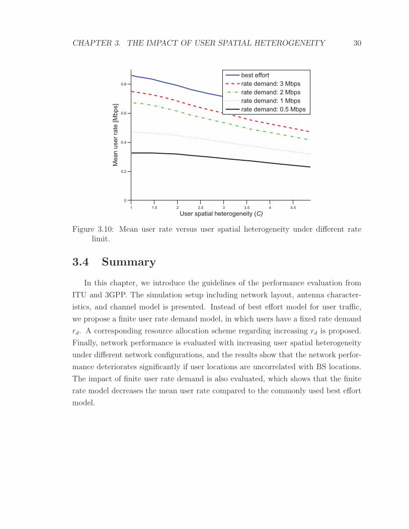
distributed picocells. Figure 3.10 shows the mean user rate versus the user spatial
heterogeneity under different rate limit. They all decrease monotonically with the
increase in user spatial heterogeneity, and the finite user rate demand decreases the
mean user rate significantly compared to the best effort model.
CHAPTER 3. THE IMPACT OF USER SPATIAL HETEROGENEITY 30
1 1.5 2 2.5 3 3.5 4 4.5
0
0.2
0.4
0.6
0.8
User spatial heterogeneity (C)
Mea
n us
er ra
te [M
bps]
best effortrate demand: 3 Mbpsrate demand: 2 Mbpsrate demand: 1 Mbpsrate demand: 0.5 Mbps
Figure 3.10: Mean user rate versus user spatial heterogeneity under different ratelimit.
3.4 Summary
In this chapter, we introduce the guidelines of the performance evaluation from
ITU and 3GPP. The simulation setup including network layout, antenna character-
istics, and channel model is presented. Instead of best effort model for user traffic,
we propose a finite user rate demand model, in which users have a fixed rate demand
rd. A corresponding resource allocation scheme regarding increasing rd is proposed.
Finally, network performance is evaluated with increasing user spatial heterogeneity
under different network configurations, and the results show that the network perfor-
mance deteriorates significantly if user locations are uncorrelated with BS locations.
The impact of finite user rate demand is also evaluated, which shows that the finite
rate model decreases the mean user rate compared to the commonly used best effort
model.

Chapter 4
Pushing Capacity Supply to Traffic
Demand
With a spatially non-uniform user distribution, some areas of the network may
have no user or only few users, and hence the resources of the BSs in those areas are
either totally wasted or underused. On the other side, the so-called hot-spot areas
may be congested with users inside suffering from low rates. One solution to this
problem is to deploy small-cells in the user hot-spots to offload traffic from macrocells.
HetNets with small-cells overlaid on macrocells have intensely been researched in
recent years, yet the distribution of small-cells is assumed to be a BPP in most of
the papers. However, given an inhomogeneously distributed set of users (as proposed
in this thesis), how to find the hot-spots from the user distribution to deploy small-
cells is a natural, yet non-trivial, question. This is especially true for the operator-
planned picocells, which are deployed by the network operators based on the traffic
distribution.
In this chapter, we first present the related work regarding the small-cell deploy-
ment (or placement) strategies, and then we propose a heuristic cluster-analysis-based
small-cell deployment method. Network performance is evaluated next with com-
parisons between the proposed small-cell deployment method and the independent
random method used in Chapter 3.
4.1 Related Work
The impact of placement of small-cells on downlink performance for cellular net-
works is evaluated in [36], in which users are deployed along the boundaries of the
31

CHAPTER 4. PUSHING CAPACITY SUPPLY TO TRAFFIC DEMAND 32
cells and the frequency reuse scheme between macrocells and microcells is studied
inside. The impact of relay station placement on the network performance in the
IEEE 802.16j network is studied in [37], in which a heuristic algorithm is proposed to
determine the number and locations of relay station deployment, with a given user
distribution and deployment budget. The user distribution is random or concentrated
in one hotspot with a certain probability. Relay deployment in cellular networks is in-
vestigated in [38], and femto-cell self-deployment in a multi-room indoor environment
is studied in [39].
The work in [40] has a similar considerations regarding small-cell deployment
with the method we proposed. In this paper, a Gibbs sampling method is proposed
to jointly optimize the locations of small-cell BSs in a multi-cell network with the
goal of maximizing any given network utility function. Both of our methods have two
considerations: (1) placing small-cells close to the high-traffic areas; and (2) avoiding
co-channel interference with the macrocells. However, the traffic in this paper is not
modeled by a general heterogeneous user distribution as in this thesis. Instead, it
is determined by a traffic profile, in which a predefined traffic density map is used.
The area of interest is a rectangular area, and is divided into a number of rectangular
mini-cells. Each mini-cell has different traffic density and the small-cells are proposed
to deployed in the centers of the mini-cells.
4.2 Cluster Analysis
The cluster analysis technique groups data into clusters such that the objects in the
same cluster are more similar to each other than to those in a different cluster. This
is a main task in data mining and has played an important role in a wide variety of
fields, including machine learning, image analysis, and information retrieval [41]. This
section uses the cluster analysis technique to find the user clusters as the potential
locations for small-cells.
4.2.1 Basic k-means Algorithm
The k-means algorithm is one of the most popular clustering algorithms used
in the cluster analysis. It is a prototype-based, partitional clustering technique that
attempts to find a user-specified number of clusters (k) represented by their centroids.

CHAPTER 4. PUSHING CAPACITY SUPPLY TO TRAFFIC DEMAND 33
The centroids are the mean of the points that belong to the cluster. The basic k-means
algorithm [41] is described below.
Algorithm Basic k-means Algorithm
1: Select k points as initial centroids.2: repeat3: Form k clusters by assigning each point to its closest centroid.4: Recompute the centroid of each cluster.5: until Centroids do not change.
4.2.2 Preprocessing and Postprocessing
As we intend to use the centroids of the clusters to deploy small-cells, outlier
users (isolated points) that are supposed to be served by macrocells are not taken
into account. We apply preprocessing to eliminate the isolated points from affecting
the locations of the centroids. A classification method of points in another density-
based clustering algorithm, DBSCAN [41], is used. All points are defined as being (1)
in the interior of a dense region (i.e., a core point), (2) on the edge of a dense region
(i.e., a border point), or (3) in a sparsely occupied region (i.e., a noise or background
point). More precisely, a point is a core point if the number of points within a certain
threshold radius of its neighborhood exceeds a certain threshold. A border point is
the point that falls within the neighborhood of a core point but that is not a core
point. A noise point is any point that is neither a core point nor a border point.
They are illustrated in Figure 4.1. After the classification, the noise points (outlier
users) are eliminated before applying the k-means algorithm. An example is shown
in Figure 4.2.
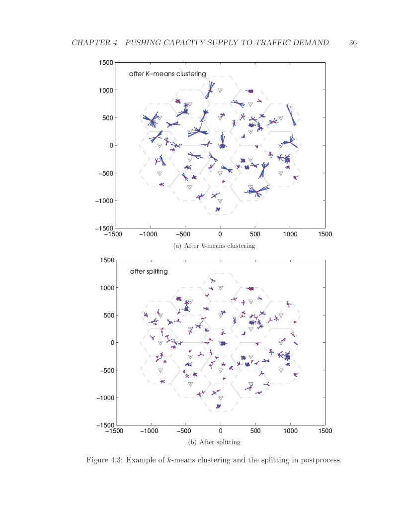
The planned number of small-cells can be used as the value of k in the k-means
algorithm. However, since the users may not naturally be clustered into k groups,
the clusters that are obtained from the k-means algorithm may turn out to be too big
for the coverage of a typical small-cell. In other words, a centroid may turn out to
be in the middle of two or more natural user clusters when k is small. A simple yet
effective way to avoid this situation is to enlarge k by splitting the clusters (by running
clustering algorithm iteratively inside the cluster), a technique that is commonly used

CHAPTER 4. PUSHING CAPACITY SUPPLY TO TRAFFIC DEMAND 34
Figure 4.1: An example of core, border, and noise points. The threshold number ofpoints is 5 in this example.
in the postprocessing for cluster analysis [41]. In our case, all clusters that have a
larger radius than the typical coverage distance of the planned small-cells are split
after the k-means clustering algorithm. After the postprocessing, k′ (greater than or
equal to k) clusters are obtained. An example of cluster splitting is shown in Figure
4.3.
4.2.3 Selection Criteria
After postprocessing, more than k clusters are obtained, potentially k′ hot-spots.
As only k small-cells are planned, a selection criterion is needed to choose k clusters
from the k′ clusters generated by the clustering algorithm.
A simple way is to determine the number of points ni in each cluster i, and then
to choose the top k out of k′ clusters with respect to the number of points in them.
However, when a cluster is close to a macrocell, a small-cell deployed in such a hot-spot
will suffer substantial interference from the macrocell in a co-channel scenario. Even
in a non-co-channel scenario, deploying small-cells close to the center of a macrocell
is not as efficient as deploying them at the edge of a macrocell, as the latter improves
the user spectral efficiency and provides more capacity at the same time.
In this thesis, we use the ratio of the distance between a user and a macrocell,
and that between a user and a potential small-cell, as a component in the objective
function to select k hot-spots from k′ clusters. We will also use the number of users

CHAPTER 4. PUSHING CAPACITY SUPPLY TO TRAFFIC DEMAND 35
(a) Original user points
(b) User points with outlier users removed
Figure 4.2: Example of noise points elimination in preprocessing of k-means.
CHAPTER 4. PUSHING CAPACITY SUPPLY TO TRAFFIC DEMAND 36
(a) After k-means clustering
(b) After splitting
Figure 4.3: Example of k-means clustering and the splitting in postprocess.

CHAPTER 4. PUSHING CAPACITY SUPPLY TO TRAFFIC DEMAND 37
criterion as the baseline method for comparison in Section 4.3. An example of cluster
selection based on the number of users in the cluster and the objective function is
shown in Figure 4.4.
Suppose that there are ni users in a cluster i; for these ni users, d(m)j and d
(s)j
represent the distances of user j to its closest macrocell, and to its cluster centroid
(the location of the planned small-cell), respectively. The proposed selection criterion
for cluster i is formulated as
Ui =1
ni
ni∑j=1
logd(m)j
d(s)j
. (4.1)
This objective function is basically derived from the Shannon formula and the path
loss expression. The goal is to select k clusters that have maximum sum user rate,∑Rj, which is proportional to the mean of the sum spectral efficiency 1
ni
∑j log(1 +
SINRj) when equal resource allocation is used. In our situation, it is reasonable
to ignore the background noise and assume a high signal-to-interference-ratio (SIR)
as users are close to the proposed small-cells. So the objective function becomes1ni
∑j log(SIRj). Let us assume that the dominant interferer, which is from the closest
macrocell, is the only interferer, and that both signal power and interference power
are calculated from the a power-law based path-loss model with the same exponent.
Then∑
j log(SIRj) becomes proportional to∑
j log(d(m)j /d
(s)j ), the sum-logarithm
of the ratio of the user to closest-macro distance to the user to planned-small-cell
distance. Since this objective function is formed under several assumptions, it is
rather approximate. However, this is not a concern, because this objective function
is not used for evaluation; it is rather used for ranking the candidates (clusters).
If interference coordination between the macrocells and the small-cells within its
coverage is used, the function can be adapted to have the second nearest neighbor
macrocell as the main interference source.
4.3 Performance Evaluation
4.3.1 Small-cell Deployment Strategy
This part evaluates the network performance with respect to user spatial hetero-
geneity under two different small-cell deployment strategies: 1) random and uniform
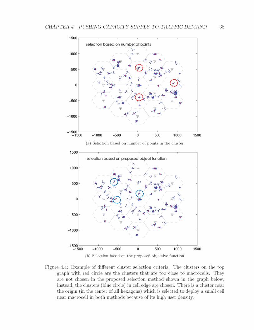
CHAPTER 4. PUSHING CAPACITY SUPPLY TO TRAFFIC DEMAND 38
(a) Selection based on number of points in the cluster
(b) Selection based on the proposed objective function
Figure 4.4: Example of different cluster selection criteria. The clusters on the topgraph with red circle are the clusters that are too close to macrocells. Theyare not chosen in the proposed selection method shown in the graph below,instead, the clusters (blue circle) in cell edge are chosen. There is a cluster nearthe origin (in the center of all hexagons) which is selected to deploy a small cellnear macrocell in both methods because of its high user density.

CHAPTER 4. PUSHING CAPACITY SUPPLY TO TRAFFIC DEMAND 39
(BPP), and 2) centroids of clusters obtained by cluster analysis. The number of pico-
cells is kept to 57 in this section. For cluster selection, two criteria are compared: the
number of users in the cluster and the proposed objective function defined in (4.1).
As we can see from Fig. 4.5, in comparison to the BPP strategy shown in the
bottom curve (identical to the middle curve in Figure 3.7), the cluster center strategy
with the proposed objective function discussed in Section 4.2.3 improves the mean
user rate by more than 50%. Besides, instead of decreasing monotonically with the
increasing user spatial heterogeneity, the mean user rate increases first and then de-
creases when cluster analysis is applied for choosing picocell locations. The cluster
center strategy performs better than the BPP strategy because of two reasons: 1) by
bringing small-cells to the centers of the traffic demand, the load among the cells be-
comes more balanced; 2) the spectral efficiency is improved since the distance between
the transmitters and receivers is shortened. However, a higher user spatial hetero-
geneity (more or larger user clusters) is beneficial to spectral efficiency improvement
with appropriately deployed small-cells, but may also make the traffic load more im-
balanced. When the traffic imbalance caused by user spatial heterogeneity outweighs
the capacities of all the small-cells, the performance goes down. This observation gives
us the insight that a certain degree of user spatial heterogeneity can be explored by
correlating the locations of users and small-cells in HetNets.
4.3.2 Fairness Index
The widely used Jain’s index is evaluated to quantify the rate fairness among all
the users. Note that the fairness evaluated here is different from the commonly used
measure that indicates whether users or applications are receiving a fair share of the
system resources. In this section, we use Jain’s index to measure the fairness of all
users in the system in terms of the rate. It is defined as
J (x1, x2, ..., xn) =(∑n
i=1 xi)2
n ·∑ni=1 x
2i
, (4.2)
where n denotes the number of users and xi denotes the user rate for user i. Figure
4.6 shows the fairness index versus user spatial heterogeneity under different network
configurations.

CHAPTER 4. PUSHING CAPACITY SUPPLY TO TRAFFIC DEMAND 40
1 2 3 4 5 6 70.3
0.4
0.5
0.6
0.7
0.8
0.9
1
1.1
1.2
1.3
Mea
n us
er ra
te [M
bps]
User spatial heterogeneity (C)
Random and uniform (BPP)
Cluster center: number of users
Cluster center: objective function
Number of picocells: 57
Figure 4.5: Mean user rate versus user spatial heterogeneity with different small-celldeployment strategies and different cluster selection methods.
1 2 3 4 5 6 70.05
0.1
0.15
0.2
0.25
0.3
0.35
0.4
0.45
0.5
0.55
Jain
’s fa
irnes
s in
dex
User spatial heterogeneity (C)
Macro + 114 pico (cluster center)
Macro−only
Macro + 114 pico (BPP)
Figure 4.6: Jain’s fairness index of user rate versus user spatial heterogeneity underdifferent network configurations.
CHAPTER 4. PUSHING CAPACITY SUPPLY TO TRAFFIC DEMAND 41
The fairness index goes down monotonically when users are more heterogeneously
distributed in the marco-only networks, and in HetNets where small-cells are ran-
domly and uniformly deployed (BPP); the Jain’s index is even worse in the latter.
The downwards trend is because of the fact that the increasing spatial heterogeneity
causes more resource imbalance. The performance gap between the macro-only net-
works and HetNets is as a result of the randomly located picocells which serve only
a small portion of the users, letting them reach high rates (which in turn worsens
the fairness index). Similar to Figure 4.5, when picocells are deployed based on the
clustering algorithm introduced in Section 4.2, the fairness index rises first and then
goes down with the increasing user spatial heterogeneity.
4.4 Summary
This section proposes the first approach to combat the traffic imbalance problem
in HetHet cellular networks (HetHetNets), which is to push capacity supply to the
traffic demand. By using the cluster analysis technique, the user cluster centers are
obtained from the non-uniform user points as the potential small-cell locations. A
selection method that considers the relative distance between user to macrocells and
user to potential small-cells is introduced to choose clusters to deploy small-cells. It
is observed that if small-cells are deployed based on the user spatial distributions, the
performance of HetNets can benefit from the increase in user spatial heterogeneity
up to a certain degree.

Chapter 5
Pushing Traffic Demand to Capacity
Supply
Other than pushing capacity supply to traffic demand as in Chapter 4, a dual
approach for load balancing with traffic shaping by user-in-loop (UIL) is introduced
in this chapter. We show that the spectral efficiency for the users and the load
balancing for the system can be improved at the same time, resulting in significant
network performance enhancement.
The rest of this chapter is organized as follows. First the related work is investi-
gated in Section 5.1, including load-aware cell association and UIL concept.
In Section 5.2, the system model for spatial traffic shaping is introduced. The
diagram inside explains how the user is incorporated as part of a closed-loop con-
trol system. A machine learning functionality is also included in the system for the
UIL controller to better predict the user behavior, which provides more relevant and
accurate suggestions.
In Section 5.3, a scenario model with two traffic classes is proposed, guaranteed
bit rate (GBR) and best effort (BE). A resource allocation scheme to guarantee the
priority of the GBR users over the BE users is also provided. Besides the traffic classes,
the spatial distribution of users is also non-uniform, modeled by a log Gaussian Cox
process introduced in Chapter 2.
In Section 5.4, the utility function for the UIL controller is introduced. Based
on the nature of the system, a sequential greedy method is used to find a suitable
location suggestion for each user, and the associated cell is generated automatically
within the algorithm.
A load-aware cell association approach for load balancing without traffic shaping
42
CHAPTER 5. PUSHING TRAFFIC DEMAND TO CAPACITY SUPPLY 43
is introduced in Section 5.5. By using the same user model and resource allocation
policy as the UIL approach, it is evaluated in comparison with the performance of
the UIL approach in the numerical analysis part, Section 5.6.
5.1 Related Work
In HetNets, due to the disparities between macrocell BSs and small-cell BSs in
terms of transmit power, antenna gain, and antenna height, the coverage sizes of
these two types of BSs are massively disparate. As such, the conventional max-SINR
(associate the user to the cell whose SINR is maximum) cell association strategy
results in significant traffic imbalance in HetNets, a major source of performance
degradation [42].
There are two possible approaches to push traffic demand to capacity supply in
load balancing: (1) users are stationary but are associated with cells by taking load
into consideration; and (2) users are a part of control loop and can be encouraged to
relocate based on the load of the cells. The first approach relates to load-aware cell
association, and the second spatial traffic shaping method is the approach we propose
in this chapter.
Recently, load-aware cell association has been considered extensively in the liter-
ature as an approach to load balancing. In this approach, users are assumed to be
stationary, and the association relation is the result of an optimization problem. The
objective of the optimization problem is usually the sum of the utility function of all
the users, and the utility function is the function of user rate in most cases, e.g., the
logarithm of user rate in [43] [44] [45]. This approach is further introduced in Section
5.5.
The UIL concept [46–54] aims at controlling the user (“layer-8”) behavior in a
wireless system to achieve a better performance of both the user and the network
by convincing the users to move from one location to a better one or to avoid traffic
congestion by postponing session traffic out of the busy hours. Based on the impact
dimension, the approach is called spatial or temporal UIL control (this work only
involves spatial UIL). In both cases, the user is within, as part of, a closed-loop
control system.
In [47], the authors show that substantial cell spectral efficiency gain is obtained
with the use of UIL. In [51], the economic aspect of the UIL concept is investigated

CHAPTER 5. PUSHING TRAFFIC DEMAND TO CAPACITY SUPPLY 44
in order to find relevant business cases for the operators and the wireless subscribers.
The proposed temporal UIL in [50] resolves congestion situations in the busy hour
and manages to let users reduce their rate of video traffic and data traffic (downloads)
because of the increased dynamic price. The approach in [50] is comparable to the
intention of the smart grid, with the additional feature of service classes. In [48], the
question about what incentives will lead to what user reaction is answered based on
survey results. Thus we are able to quantitatively describe the user behavior in a
system theoretic framework.
Under the concept of the UIL, this thesis goes further with a utility function that
incorporates cell-level load factor, potential SINR and the user moving probability,
which leads to a novel spatial traffic shaping approach to load balancing.
5.2 System Model for Spatial Traffic Shaping
Under the paradigm of UIL, users are suggested opportunistically to move to a
new location according to operator recommendation and incentive displayed on the
user terminal. Users can choose to or not to comply with the suggestion for better
service and better rewards (depending on the content of the incentive). In this thesis,
the new location is the place where the user will receive higher SINR and/or more
resource share, and the user is willing to move to. It is given by the UIL controller
(see Figure 5.1) based on the utility function, which considers SINR maps of all cells
(the potential spectral efficiencies of the new locations with different cells), the load
factor of each cell and the probability of moving to different locations (related to
application class, user behavior and so on). Load balancing is achieved by the spatial
movement of users which comply with the suggestions. By shaping the traffic spatial
distribution, the traffic demand is controlled to meet the capacity supply better, the
distribution of which usually stays unchanged once the placement of BSs has been
completed.
The UIL system theoretic model for traffic shaping is shown in Figure 5.1. Instead
of assuming users being a traffic generator and consumer as a black box only, the UIL
framework allows a control input into the user block, on which the user receives
suggestions and incentives (i.e., progressive tariffs, reward points, higher access rates,
or even environmental indicators) in order to convince him to move to a new location.
The control information (CI) is sent from the UIL controller in form of suggestions

CHAPTER 5. PUSHING TRAFFIC DEMAND TO CAPACITY SUPPLY 45
Figure 5.1: The UIL system theoretic model diagram. The UIL system theoreticmodel is a closed loop with the user included in the system to control. Theuser’s output is the action of complying or not with the suggestions. As wehave multiple users in a cell, the arcs between controller, user, and the systemare vectorized for m users.
on the user terminal graphical interface (e.g., a map with directions). The suggestion
is opportunistic (not mandatory) and users can choose to comply or not. The action
of the users (cooperate or not) is then returned to the cellular network system. The
suggestions are the main output of the UIL controller based on the utility function
discussed in Section 5.4, and the incentive is set by the operator considering factors
like the current tariffs, the marketing policy, the network congestion degree, and so
on.
The input of the UIL controller includes three components which are: 1) the map
information from the database, 2) the user probability of moving, P , from the user
behavior learning center, and 3) the cell load information, L, from the cellular network
system. The map information includes city map that facilitates the movement of users
and the spectral efficiency map used to calculate the utility function. The spectral
efficiency map is generated from the network with the measurement from all the
user terminals being accumulated and statistically averaged. It is relatively constant
and only needs to be updated when the network configuration or the city landscape
changes.
P is the output of the user behavior learning center, which learns the user behavior
under different circumstances. For example, the probability of user u with quality of
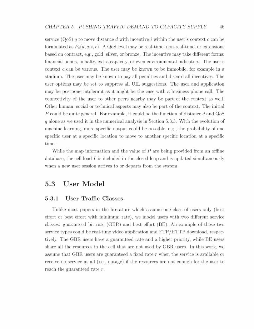
CHAPTER 5. PUSHING TRAFFIC DEMAND TO CAPACITY SUPPLY 46
service (QoS) q to move distance d with incentive i within the user’s context c can be
formulated as Pu(d, q, i, c). A QoS level may be real-time, non-real-time, or extensions
based on contract, e.g., gold, silver, or bronze. The incentive may take different forms:
financial bonus, penalty, extra capacity, or even environmental indicators. The user’s
context c can be various. The user may be known to be immobile, for example in a
stadium. The user may be known to pay all penalties and discard all incentives. The
user options may be set to suppress all UIL suggestions. The user and application
may be postpone intolerant as it might be the case with a business phone call. The
connectivity of the user to other peers nearby may be part of the context as well.
Other human, social or technical aspects may also be part of the context. The initial
P could be quite general. For example, it could be the function of distance d and QoS
q alone as we used it in the numerical analysis in Section 5.3.3. With the evolution of
machine learning, more specific output could be possible, e.g., the probability of one
specific user at a specific location to move to another specific location at a specific
time.
While the map information and the value of P are being provided from an offline
database, the cell load L is included in the closed loop and is updated simultaneously
when a new user session arrives to or departs from the system.
5.3 User Model
5.3.1 User Traffic Classes
Unlike most papers in the literature which assume one class of users only (best
effort or best effort with minimum rate), we model users with two different service
classes: guaranteed bit rate (GBR) and best effort (BE). An example of these two
service types could be real-time video application and FTP/HTTP download, respec-
tively. The GBR users have a guaranteed rate and a higher priority, while BE users
share all the resources in the cell that are not used by GBR users. In this work, we
assume that GBR users are guaranteed a fixed rate r when the service is available or
receive no service at all (i.e., outage) if the resources are not enough for the user to
reach the guaranteed rate r.

CHAPTER 5. PUSHING TRAFFIC DEMAND TO CAPACITY SUPPLY 47
5.3.2 Resource Allocation
We denote by C the set of all cells (including macrocells and small-cells). The total
resources of a cell j ∈ C, denoted by Wj, are shared among all the users associated
with it. The resources can be time or frequency slots, or both. In our model, GBR
users have higher priority and are allocated the exact amount of resources they need.
For a GBR user i with spectral efficiency sij from cell j, the amount of resources
needed from cell j to reach the guaranteed rate r is
wij =r
sij. (5.1)
sij is derived from the Shannon formula,
sij = log
(1 +
Pjgij∑h∈C,h �=j Phgih + σ2
), (5.2)
where Pj is the transmit power of cell j, gij denotes the channel gain between user i
and cell j. The channel gain includes antenna gain, path loss and shadowing. Fast
fading is not considered here as an averaged SINR is assumed over the session length.
σ2 represents the noise power in SINR.
When a new GBR user i arrives to cell j, the user will be allocated the exact
amount of resources wij that is needed if
Wj −∑
i′∈Ug(i)
ai′jwi′j > wij, (5.3)
where Wj is the total resources of the cell j. ai′j is the association indicator (i.e.,
ai′j = 1, if user i′ is associated with cell j, ai′j = 0 otherwise) and Ug(i) is the set
of the existing GBR users at the moment when user i arrives to the system. If the
Inequality (5.3) does not hold, this GBR user will be blocked, which results in the
outage of this GBR user.
The BE users equally share the remaining resources that are not used by the GBR
users. For example, when a new BE user k arrives to the system, the resources will
be reallocated to these nbj(k) + 1 users, where nb
j(k) is the number of the existing
BE users associated with cell j at the moment when user k arrives. The amount of
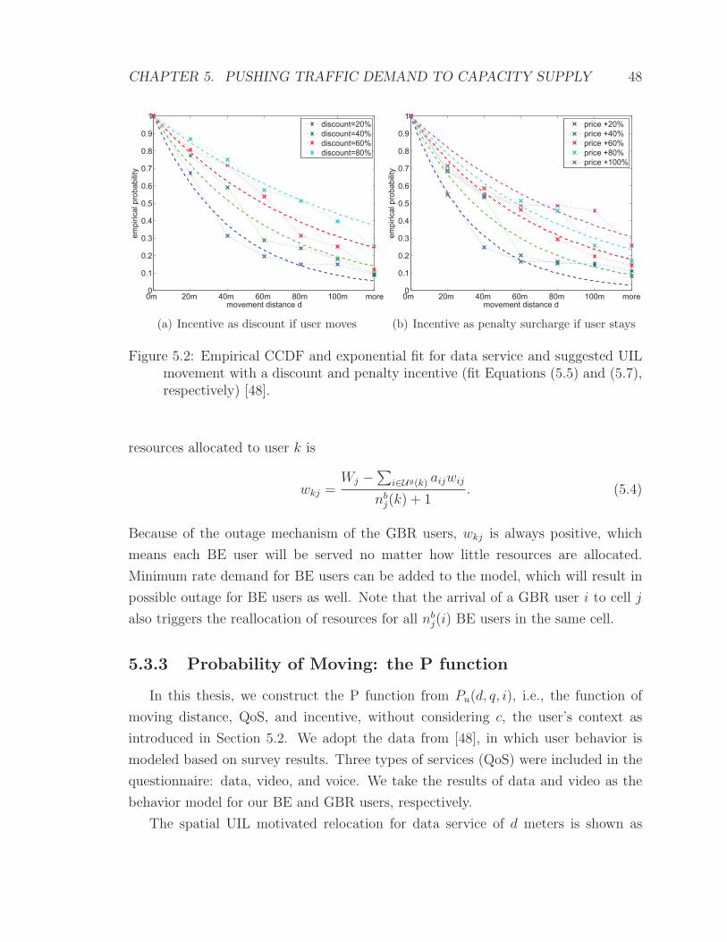
CHAPTER 5. PUSHING TRAFFIC DEMAND TO CAPACITY SUPPLY 48
0m 20m 40m 60m 80m 100m more0
0.1
0.2
0.3
0.4
0.5
0.6
0.7
0.8
0.9
1
movement distance d
empi
rical
pro
babi
lity
discount=20%discount=40%discount=60%discount=80%
(a) Incentive as discount if user moves
0m 20m 40m 60m 80m 100m more0
0.1
0.2
0.3
0.4
0.5
0.6
0.7
0.8
0.9
1
movement distance d
empi
rical
pro
babi
lity
price +20%price +40%price +60%price +80%price +100%
(b) Incentive as penalty surcharge if user stays
Figure 5.2: Empirical CCDF and exponential fit for data service and suggested UILmovement with a discount and penalty incentive (fit Equations (5.5) and (5.7),respectively) [48].
resources allocated to user k is
wkj =Wj −
∑i∈Ug(k) aijwij
nbj(k) + 1
. (5.4)
Because of the outage mechanism of the GBR users, wkj is always positive, which
means each BE user will be served no matter how little resources are allocated.
Minimum rate demand for BE users can be added to the model, which will result in
possible outage for BE users as well. Note that the arrival of a GBR user i to cell j
also triggers the reallocation of resources for all nbj(i) BE users in the same cell.
5.3.3 Probability of Moving: the P function
In this thesis, we construct the P function from Pu(d, q, i), i.e., the function of
moving distance, QoS, and incentive, without considering c, the user’s context as
introduced in Section 5.2. We adopt the data from [48], in which user behavior is
modeled based on survey results. Three types of services (QoS) were included in the
questionnaire: data, video, and voice. We take the results of data and video as the
behavior model for our BE and GBR users, respectively.
The spatial UIL motivated relocation for data service of d meters is shown as

CHAPTER 5. PUSHING TRAFFIC DEMAND TO CAPACITY SUPPLY 49
complementary cumulative distribution function (CCDF) in Figure 5.2, first with a
discount incentive δ and second with a surcharge penalty π. i is the corresponding
integer index. The results show a clear control ratio. The numeric fits for the data
service (BE users) are as follows [48]:
δi=1 = −20% ⇒ p = e−0.0244·d
δi=2 = −40% ⇒ p = e−0.0164·d
δi=3 = −60% ⇒ p = e−0.0117·d
δi=4 = −80% ⇒ p = e−0.0082·d
(5.5)
p = e(−0.0285+0.0053·i)·d = e(−0.0285−0.0265·δ)·d (5.6)
πi=1 = +020% ⇒ p = e−0.0291·d
πi=2 = +040% ⇒ p = e−0.0202·d
πi=3 = +060% ⇒ p = e−0.0144·d
πi=4 = +080% ⇒ p = e−0.0121·d
πi=5 = +100% ⇒ p = e−0.0099·d
(5.7)
p = e(−0.0311+0.0047·i)·d = e(−0.0311−0.0235·π)·d (5.8)
The spatial UIL motivated relocation for video service of d meters is shown as
complementary cumulative distribution function (CCDF) in Figure 5.3, first with a
discount incentive δ and second with a surcharge penalty π. The numeric fits for the
video service (GBR users) are as follows [48]:
δi=1 = −20% ⇒ p = e−0.0276·d
δi=2 = −40% ⇒ p = e−0.0192·d
δi=3 = −60% ⇒ p = e−0.0127·d
δi=4 = −80% ⇒ p = e−0.0090·d
(5.9)
p = e(−0.0327+0.0062·i)·d = e(−0.0327−0.0310·δ)·d (5.10)

CHAPTER 5. PUSHING TRAFFIC DEMAND TO CAPACITY SUPPLY 50
0m 20m 40m 60m 80m 100m more0
0.1
0.2
0.3
0.4
0.5
0.6
0.7
0.8
0.9
1
movement distance d
empi
rical
pro
babi
lity
discount=20%discount=40%discount=60%discount=80%
(a) Incentive as discount if user moves
0m 20m 40m 60m 80m 100m more0
0.1
0.2
0.3
0.4
0.5
0.6
0.7
0.8
0.9
1
movement distance d
empi
rical
pro
babi
lity
price +20%price +40%price +60%price +80%price +100%
(b) Incentive as penalty surcharge if users stays
Figure 5.3: Empirical CCDF and exponential fit for video service and suggested UILmovement with a discount and penalty surcharge incentive (fit Equations (5.9)and 5.11, respectively) [48].
πi=1 = +020% ⇒ p = e−0.0328·d
πi=2 = +040% ⇒ p = e−0.0234·d
πi=3 = +060% ⇒ p = e−0.0176·d
πi=4 = +080% ⇒ p = e−0.0129·d
πi=5 = +100% ⇒ p = e−0.0123·d
(5.11)
p = e(−0.0352+0.0051·i)·d = e(−0.0352−0.0255·π)·d (5.12)
More information can be found in [48]. All the results confirm the general intuitive
trends:
• The acceptance p drops with effort (distance d in spatial domain as the case in
this thesis).
• A stronger incentive is followed with more acceptance.
• A more forceful penalty also leads to more obedience.
5.4 Proposed UIL Load Balancing Approach
The UIL controller outputs the control information with the suggestion of the
potential location based on the maximization of a utility function. The objective

CHAPTER 5. PUSHING TRAFFIC DEMAND TO CAPACITY SUPPLY 51
utility function combines three factors: the SINR value of different locations from
each cell, the load of each cell, and the probability of moving from the current location
to the potential locations.
Note that the utility function formulated in this section is just one way to combine
all the three factors that are considered in this thesis. In our formulation, all the three
factors are treated equally, i.e., they are of the same order in the function. Other
formulations are also possible.
5.4.1 Utility Function of GBR Users
The utility function of a GBR user i with cell j is formulated as
Uij(x, y) = pi(x, y) · sj(x, y) · (1− ρbj(i)), (5.13)
where pi(x, y) is the probability of user i moving from his current location to the new
location with coordinates (x, y), sj(x, y) is the spectral efficiency map of cell j, and
ρbj(i) ∈ [0, 1] is the load factor of cell j for the existing GBR users at the moment
when user i arrives to the system. ρbj(i) is defined as
ρbj(i) =
∑i′∈Ug(i) ai′jwi′j
Wj
, (5.14)
where ai′j is a known matrix indicating the association relation of all the GBR users
at the moment when user i arrives to the system, and is updated each time after a
new user’s decision is made.
So for each new user arriving to the system, we get a three dimensional matrix.
The first dimension is the cell index, and the other two dimensions are the coordinates
of the map.
5.4.2 Utility Function of BE Users
The utility function of the BE users is similar to that of the GBR users, except
the load factor. The utility function of a BE user k with a cell j ∈ C is formulated as
Ukj(x, y) = pk(x, y) · sj(x, y) ·(1− ρbj(k))
nbj(k) + 1
, (5.15)

CHAPTER 5. PUSHING TRAFFIC DEMAND TO CAPACITY SUPPLY 52
where ρbj(k), as defined in (5.14), is the load factor of cell j of existing GBR users
when the BE user k arrives to the system. nbj(k) is the number of the BE users in
cell j when user k arrives to the system.
5.4.3 Sequential Optimization
Due to the fact that each user, or more precisely, each session, arrives to the
system sequentially and it is inappropriate to suggest a user to move more than once
during one data session, we use a greedy algorithm to optimize the utility function for
each user sequentially based on the network situation at the moment the user arrives.
Another benefit of the sequential optimization in this system is that the system knows
the actions of the preceding users, or the system can predict their actions based on
their probabilities of moving obtained from the completed optimization problems.
Different from dynamic programming, the algorithm never reconsiders its choices,
i.e., a user will not receive a second suggestion during one data session even though
the network load has changed (and it may be better to move to another location)
after he receives the first suggestion.
For a new GBR user i, we conduct a exhaustive search on the utility function
Uij(x, y) of all the cells and locations based on the current load information. The
optimization problem is formulated as
maxj,x,y
Uij(x, y)
s.t. Wj −∑
i′∈Ug(i)
ai′jwi′j >r
sj(x, y)
x ∈ [0, X]
y ∈ [0, Y ]
j ∈ C,
(5.16)
where x and y take discrete values from the range X and Y based on the resolutions
of the map. The matrix ai′j, which shows the association relation of all the existing
GBR users to the associated cells at the moment the user i arrives to the system, is
a know matrix for each new user. The exhaustive search over the three dimensional
matrix provides the optimal value for U� for user i and the corresponding values of
the variables, i.e., the optimal associated cell j� and the optimal location (x�, y�).
The probability of user i to move to the optimal location (x�, y�) is obtained from

CHAPTER 5. PUSHING TRAFFIC DEMAND TO CAPACITY SUPPLY 53
the P function of this user, pi(x�, y�), which we denote as p�i .
The first constraint in the problem guarantees that there are enough resources
in the potential cell for user i to reach rate r. If no cell is feasible because of the
constrain, it means there is no location in any cells that can provide the spectral
efficiency and the required resources to make this user reach the guaranteed bit rate,
or such a location does exist yet this user has zero probability to move there based
on our P function (e.g., too far from the current location), an outage of this GBR
user happens and no suggestion will be given.
As users only have probabilities to move within a short distance, i.e., p(i, j) equals
to zero if the potential locations are far from the users, so it is realistic for the UIL
controller to do the exhaustive search over all of the cells in a very short time and to
provide suggestions to each user when the sessions start.
The optimization problem for the BE users is similar to the GBR users except
that it comes without the first constraint that guarantees the amount of resources
available as in (5.16).
In the simulation, the action of the user can be modeled as a Bernoulli trial. A
random number between 0 and 1 is generated and is compared to the p�i . This user
moves if the random number is smaller than p�i , stays otherwise. If user i complies
with the suggestion, the location of this user will be changed to (x�, y�), and cell j�
will be assigned as the associated cell for this user, i.e., aij� = 1. If the user chooses
to stay without moving, he will be associated with the cell that provides the best
SINR value. After the decision is made for each user, the association matrix ai′j is
updated as an input to calculate the load factor for the next user.
5.4.4 An Example of Load Balancing Achieved by UIL
In this section, we provide an example of a typical user associating with a cell based
on the previously introduced utility function. A user is located as shown by the red
cross in Figure 5.4 (a), and the probabilities of this user to move from the current
location to other locations are shown in 5.4 (b). The probability P is calculated from
Equation (5.9). A max-spectral-efficiency map is shown in Figure 5.4 (c), where each
pixel is represented by the maximum value out of the spectral efficiencies received
from all the cells, including macrocells and small-cells. Correlated shadowing for
macrocells is used in the serving area and the log-normal shadowing is used in the
wrap-around area. No shadowing is applied to small-cells. This map provides the

CHAPTER 5. PUSHING TRAFFIC DEMAND TO CAPACITY SUPPLY 54
natural selection of cell to associate with by the cell index from argmax(spj), where
spj is the spectral efficiency of pixel p from cell j.
Based on the spectral efficiency map in Figure 5.4 (c), this user will associate
with the macrocell A (as shown by the arrow in Figure 5.4 (a)) if best-SINR is the
association strategy. If we multiply the P map with the max-spectral-efficiency map,
i.e., without considering the load of cells, the user will be suggested to move to the
small-cell B in the map.
By multiplying the spectral efficiency map of each cell, the load of each cell, and
the probability of moving map of this user, we get a 3D utility map. To show the
results in a 2D map, we represent each pixel with the maximum value of all the
utilities among all the cells at each pixel, which is shown in Figure 5.4 (d).
From Figure 5.4 (d), we can see that cell B has very low utility and cell C and cell
D have the highest utility. The high load is the reason why the utility of small-cell B
becomes low. The user will be suggested to move to small-cell C or D according to
the max-utility map in Figure 5.4 (d).
5.4.5 Outlook: Include Mobility Model
If a user mobility model is included in the system, Equation (5.14) should be
modified to include network load variation during the time period that the current
user is moving to the potential location. For example, when a new user i arrives to
the system at time t, the loads of the potential cells used in the utility function are
not the loads at the moment t, ρj(t), j ∈ C, but the load at the moment when user
i arrives to the potential cell, ρj(t + τj), j ∈ C, where τj is the time needed for user
i to move to cell j. The users considered in the load ρj(t + τj) should include the
coming users and exclude the leaving users during the time interval τj for each cell
j. With the probabilities of moving of the existing users available, the numerator in
Equation (5.14) is then changed to the expected value of the resources consumed by
the existing and the potential users.
5.5 Load-Aware Cell Association
In this section, we develop a baseline load balancing approach without involving
users’ movement. Users are associate with cells not purely based on the received

CHAPTER 5. PUSHING TRAFFIC DEMAND TO CAPACITY SUPPLY 55
−1500 −1000 −500 0 500 1000 1500−1500
−1000
−500
0
500
1000
1500
x
y
AB
CD
(a) User location
−1500 −1000 −500 0 500 1000 1500−1500
−1000
−500
0
500
1000
1500
x
y
0
0.1
0.2
0.3
0.4
0.5
0.6
0.7
0.8
0.9
(b) Probability of moving
−1500 −1000 −500 0 500 1000 1500−1500
−1000
−500
0
500
1000
1500
x
y
0.5
1
1.5
2
2.5
3
3.5
4
4.5
5
(c) Max-spetral-efficiency map
−1500 −1000 −500 0 500 1000 1500−1500
−1000
−500
0
500
1000
1500
x
y
0
0.05
0.1
0.15
0.2
(d) Max-utility map
Figure 5.4: An example of load balancing achieved by UIL. The location of the user isshown in (a) as a red cross. The probability map of moving to other locations forthis user in shown in (b). The user will associate will the macrocell A (shownas an arrow in (a)) if best-SINR is the association strategy according to themax-spectral-efficiency map in (c). The user will be suggested to move to thesmall-cell B if load is not considered. If we use the utility function defined inthis thesis, the user will be suggested to move to the small-cell C or D accordingto the max-utility map in (d). The small-cell B has very low utility because ithas a high load.

CHAPTER 5. PUSHING TRAFFIC DEMAND TO CAPACITY SUPPLY 56
SINR, but also on the load of each cell. To some extent, this is also an approach to
push capacity supply to traffic demand through the process of cell association, known
as load-aware cell association. Load-aware cell association has been researched in the
literature intensively as an approach to perform load balancing, yet only one class of
users is assumed (in most cases, best effort users). In this section, we formulate the
load-aware association problem with the same user model and the same optimization
method as in the UIL approach. The performance comparison with the UIL approach
is provided in the next section.
5.5.1 Related Work
In [55], the handoff and cell association are formulated into an iterative optimiza-
tion problem and solved with a distributed load-awareness scheme. In [43] and [45],
with the utility function of the long-term user rate as the objective, the duality the-
ory in optimization is used to tackle the cell association problem. The distributed
solutions inside interpret the loads as the price of the BSs, which lead to a more
balanced traffic load compared to the SINR-based cell association. In [56], a heuristic
solution to the joint problem of cell association and linear beamformer design in a
MIMO HetNets is given.
A typical load-aware cell association optimization problem [43] [45] is defined as
maxaij ,nj
∑i,j
aij log
(Wj
nj
log(1 + sij)
)
s.t.∑j
aij = 1
∑i
aij = nj
∑j
nj = N
aij ∈ 0, 1,
(5.17)
where nj is the number of users associated with cell j, and N is the total number
of users in the system. In this formulation, the objective is the sum of each user’s
utility, log(rij), where rij is the rate of user i with cell j calculated from the Shannon
formula. The log-utility is a proportionally fair function, which encourages allocating
more resources to the low-rate users. In other words, this property encourages load

CHAPTER 5. PUSHING TRAFFIC DEMAND TO CAPACITY SUPPLY 57
balancing. The authors in [43] claim that the optimal resource allocation strategy is
equal allocation when log-utility is adopted, which is the reason why each user gets
the amount ofWj
njresources in Equation (5.17).
As mentioned before, only best effort users are modeled in this optimization prob-
lem, and resources are equally allocated among all users. To be comparable with
the UIL approach we proposed in the previous section, we reformulated the load-
aware association problem in the next section with the user model and the resource
allocation scheme we defined in Section 5.3.
5.5.2 Proposed Scheme
Similar to the utility function defined for the UIL scheme, we define the util-
ity functions for GBR users and BE users separately for load-aware cell association
scheme. Without including the user moving, only two factors are considered in the
function, the spectral efficiency and the load of the potential cell. The utility function
of a GBR user i with a cell j is defined as
Uij = sij · (1− ρbj(i)), (5.18)
where sij denotes the spectral efficiency of cell j at the current location of user i, and
ρbj(i) has the same definition as in the UIL scheme, the load of GBR users of cell j
when user i arrives to the system. Similarly, the utility function of a BE user k with
a cell j is defined as
Ukj = skj ·(1− ρbj(k))
nbj(k) + 1
. (5.19)
For each new GBR user, an exhaustive search is conducted on all the cells to find
the maximum utility defined in (5.18). The optimization problem is formulated as
maxj
Uij
s.t. Wj −∑
i′∈Ug(i)
ai′jwi′j > wij
j ∈ C
(5.20)
The GBR user i is associated to j� from this optimization problem, or associated
to the best-SINR cell if there is no cell feasible. The association matrix aij is updated

CHAPTER 5. PUSHING TRAFFIC DEMAND TO CAPACITY SUPPLY 58
Table 5.1: Simulation parameters in Chapter 5
Parameter Assumption
Macrocell layout Hexagonal grid of 19 × 3 = 57 macrocells
Picocell layout 57 × 2 = 114 picocells (BPP)
Minimum distance between picocells 40 m
Average user number 10 users / cell × 171 cells = 1710 users
Average session length 300 s
Guaranteed bit rate for GBR users 1 Mbps
Percentage of GBR users 50 %
System bandwidth 10 MHz (FDD) at 2 GHz
Shadowing Log-normal, s.d. 4 for LOS, 6 for NLOS
Macrocell Tx power 46 dBm
Picocell Tx power 37 dBm
Antenna gain Macrocell: 17 dBi, picocell: 5 dBi
Traffic model BE and GBR
after each user’s associated cell is obtained.
For a BE user k, the associated cell is argmaxj Ukj with no constrains.
5.6 Numerical Results
5.6.1 Simulation Setup
In this simulation, ITU urban macrocell (UMa) [57] and 3GPP case 6.2 in release
9 [18] is the scenario used for HetNets. 19 macrocells sites, each of 3 cells with inter
site distance (ISD) of 500 meters, are configured in the system. The locations of the
macrocell sites are fixed and form a hexagonal grid layout. The HetNets consists
of two tiers with outdoor picocells overlaid on the same area of macrocells. The
distribution of picocells is random and uniform. A wrap-around technique is applied
on both macro and small-cells to eliminate the boundary effect.
The channel follows the model 2 in [18] for both macrocells and outdoor pico-
cells, in which a LOS and NLOS power-law path loss model is used. The downlink

CHAPTER 5. PUSHING TRAFFIC DEMAND TO CAPACITY SUPPLY 59
signal experiences path loss and shadowing, while the fast fading is assumed to be
averaged out. The shadowing is correlated based on the models used in [58] [59].
An illustration of the correlated shadowing can be found in Figure 5.4 (c). The user
rate is calculated from the product of resource allocated and the spectral efficiency
reached, both of which are defined in Section 5.3.2. A user suffers interference from
all the macrocells and picocells outside its own serving cell (which may be a macro-
cell or a picocell). Both macrocells and picocells share the same bandwidth, and no
interference coordination or cancellation technique is used. Table 5.1 shows the key
parameters used in the simulations.
Users arrive the system according to a Poisson process and leave the system after
a session length. In each drop of the simulation, the system starts from zero users.
Section 5.6.2 defines the transient and steady state of the simulation, and the per-
formance evaluation inside is time-dependent. After that, all the performances are
evaluated based on the snapshots of the system when the user number is in steady
state, and each snapshot is taken from an individual drop, i.e., the snapshots are
totally independent.
The metrics are evaluated with respect to the increasing spatial traffic demand
heterogeneities under three scenarios: (a) no load balancing with best-SINR associ-
ation strategy, (b) load balancing approach with load-aware association strategy as
introduced in Section 5.5, and (c) load balancing approach with the UIL scheme.
We change the value of σ in LGCP to get user distributions with different spatial
heterogeneities, which are measured by C, the normalized CoV of Voronoi cell area
in the Voronoi tessellations of the user points [24]. When C is equal to 1, the user
distribution forms a PPP.
In the UIL scheme, the probability of moving p is the function of user traffic
class (GBR or BE) and the moving distance. We adopt the result in [48], in which
exponential functions for different traffic classes with respect to moving distances are
obtained based on a survey result. The functions are shown in Section 5.3.3. In this
thesis, we use the discount as the incentive method, and the incentive index is fixed
at 4, which is 80% discount if a user complies with the suggestion. Further work
regarding different levels of incentive can be included. For a user, GBR or BE, the
probability of moving p� is derived from the distance between the current location
and the optimal location (x�, y�). A Bernoulli trial is then conducted to determine
whether this user complies with the suggestion or not. If complies, the user will be

CHAPTER 5. PUSHING TRAFFIC DEMAND TO CAPACITY SUPPLY 60
0 1000 2000 3000 4000 50000
200
400
600
800
1000
1200
1400
1600
1800
Num
ber o
f use
rs
Time (s)
Transient state Steady state
Figure 5.5: The number of users in the system over time in one drop.
relocated to (x�, y�) and associated with cell j� as discussed in Section 5.4.3. If not,
the user will associate with a cell based on the best-SINR policy.
5.6.2 Transient and Steady State Behavior
The system starts from zero users, and users arrive to the system with exponential
inter-arrival time. We fix the session length at 300 seconds, and users leave the system
after the session expires. In the steady state, the average user number is 1710, i.e.,
10 users per cell. Based on the queue theory, the arrival rate and the departure rate
are calculated from the average number of users divided by the session length.
The system starts from transient state till the number of users reaches in a certain
probability of error regarding to the average user number. Figure 5.5 shows the num-
ber of users changing over time and the transient time accordingly. An exponential
fitting with coefficient λ can be found from the nonlinear regression of the curve in
5.5. The transient time τ is calculated from the equation 1 − e−λτ = 1 − ε, where
ε is the probability of error. In this simulation, we take ε as 1%. Other statistics

CHAPTER 5. PUSHING TRAFFIC DEMAND TO CAPACITY SUPPLY 61
0 1000 2000 3000 4000 500010
15
20
25
30
35
40
45
50C
ondi
tiona
l mea
n of
mov
ing
dist
ance
in U
IL (m
)
Time (s)
(a) Average moving distance
0 1000 2000 3000 4000 50000
0.1
0.2
0.3
0.4
0.5
0.6
0.7
0.8
0.9
1
Pro
babi
lity
of m
ovin
g in
UIL
Time (s)
(b) Average moving probility
Figure 5.6: Statistics of user movement over time.
including average moving distance (conditional, only the users that move are consid-
ered) and the moving probability are shown in Figure 5.6. As we can see from Figure
5.6, the average moving distance is about 43 meters, and the probability of moving
is about 0.7, which complies with the curves in Figure 5.2 (a) with 80% discount as
the incentive.
The user spatial heterogeneity (CoV) is evaluated with and without UIL. As we
can see from Figure 5.7, the CoV of user spatial distribution is lower in the UIL
scheme. This is due to the fact that UIL suggest users to move to the less loaded cell,
which helps to reduce the degree of user spatial heterogeneity.
The performances hereafter are evaluated based on the snapshots of the system
when the user number is in steady state, and each snapshot is taken from an inde-
pendent drop.
5.6.3 Loads among Different Cells
The load factor of GBR users is defined as ρ in Equation (5.14) in Section 5.4.1.
If we take the standard deviation of ρj (j ∈ C), denoted as stdρ, it can be used as a
measure to indicate the degree of network-wide load balance. The lower the stdρ is, the
more balanced the network is. Figure 5.8 shows the stdρ with respect to user spatial
heterogeneities under different load balancing strategies. First, it is obvious that the

CHAPTER 5. PUSHING TRAFFIC DEMAND TO CAPACITY SUPPLY 62
0 1000 2000 3000 4000 50000
0.2
0.4
0.6
0.8
1
1.2
1.4
1.6
1.8
2
Use
r spa
tial h
eter
ogen
eity
leve
l (C
oV)
Time (s)
without UILwith UIL
Figure 5.7: The CoV of user spatial distribution over time with and without UIL.

CHAPTER 5. PUSHING TRAFFIC DEMAND TO CAPACITY SUPPLY 63
1 1.2 1.4 1.6 1.8 20.4
0.6
0.8
1
1.2
1.4
1.6
1.8
Sta
ndar
d de
viat
ion
of ρ
for a
ll ce
lls
User spatial heterogeneity level (CoV)
best−SINRload−aware associationUIL
Figure 5.8: The standard deviation of GBR user load (ρ) of all the cells with respectto user spatial heterogeneities under different load balancing strategies.
network is becoming more imbalanced when the user spatial heterogeneity (traffic
demand heterogeneity) increases in all the three schemes. Second, as we can see, stdρ
is the lowest in the UIL scheme, highest in the best-SINR scheme, and the load-aware
cell association scheme is in the middle, which shows that the UIL approach improves
network-wide load balance substantially, and the load-aware association approach is
also an effective approach to do load-balancing compare to the best-SINR strategy
without load balancing.
5.6.4 GBR Users Outage
As shown in Figure 5.9, the outage percentage is the lowest (best) with the UIL
scheme and the highest (worst) with the best-SINR strategy. The load-aware asso-
ciation strategy as an approach to load balancing without the involvement of user
relocation performs in the middle. The outage percentages rise quickly with the in-
crease of user spatial heterogeneity (i.e., traffic demand heterogeneity) in all the three
strategies.

CHAPTER 5. PUSHING TRAFFIC DEMAND TO CAPACITY SUPPLY 64
1 2 3 4 5 60
10
20
30
40
50
60
70
80
GB
R u
ser o
utag
e pe
rcen
tage
(%)
User spatial heterogeneity level (CoV)
best−SINRload−aware associationUIL
Figure 5.9: The outage percentage of GBR users with respect to user spatial hetero-geneities under different load balancing strategies. Each dot, cross, and plussign represents the result of a simulation drop in best-SINR, load-aware cellassociation and UIL scheme, respectively. The lines are the polynomial curvefitting with n = 3.

CHAPTER 5. PUSHING TRAFFIC DEMAND TO CAPACITY SUPPLY 65
1 2 3 4 5 60.2
0.3
0.4
0.5
0.6
0.7
0.8
0.9
1
Mea
n th
roug
hput
of G
BR
use
rs (b
ps)
User spatial heterogeneity level (CoV)
best−SINRload−aware associationUIL
Figure 5.10: Mean rate of all the GBR users in the system with respect to user spatialheterogeneities under different load balancing strategies. Each dot, cross, andplus sign represents the result of a simulation drop in best-SINR, load-aware cellassociation and UIL scheme, respectively. The lines are the polynomial curvefitting with n = 3.
The reason is when the user spatial heterogeneity increases, the traffic demand
may be highly clustered in some areas that exceed the capacities of the associated
cells, which results in higher GBR user outage. Load-aware cell association strategy
takes the load factor into consideration, and thus performs better than the best-SINR
strategy without load balancing. The UIL scheme outperforms the load-aware asso-
ciation by combining spatial relocation (with probability) and load factor together.
5.6.5 Mean User Rate
The mean user rates of GBR users and BE users are calculated separately as shown
in Figure 5.10 and Figure 5.11, respectively. They all have the same downward trends
with the increase of user spatial heterogeneity. For GBR users, the UIL scheme
performs the best, the load-aware association strategy comes next, and the best-
SINR strategy with no load balancing performs the worst. This can be explained

CHAPTER 5. PUSHING TRAFFIC DEMAND TO CAPACITY SUPPLY 66
1 2 3 4 5 60
0.5
1
1.5
2
2.5
3
3.5
4
Mea
n th
roug
hput
of B
E u
sers
(bps
)
User spatial heterogeneity level (CoV)
best−SINRload−aware associationUIL
Figure 5.11: Mean rate of all the BE users in the system with respect to user spatialheterogeneities under different load balancing strategies. Each dot, cross, andplus sign represents the result of a simulation drop in best-SINR, load-aware cellassociation and UIL scheme, respectively. The lines are the polynomial curvefitting with n = 3.
with the same reason mentioned for the outage percentage. However, for BE users,
the UIL scheme still performs the best but the load-aware cell association strategy
does not surpass the best-SINR strategy. This is due to the fact that the load-
aware strategy may associate a GBR user to a lightly loaded neighbor cell with lower
spectral efficiency received, which results in a higher resource consumption. Because
of the priority of GBR users, less resources are left for BE users, which brings a worse
performance for the load-aware association strategy in terms of mean user rate.
5.6.6 Fairness Index
As in Section 4.3.2, we use Jain’s index to measure the fairness of user rate.
Different from Section 4.3.2, GBR users and BE users are evaluated separately. Figure
5.12 and Figure 5.13 show the fairness index of GBR user rate and BE user rate versus
user spatial heterogeneity under different network configurations, respectively. Similar

CHAPTER 5. PUSHING TRAFFIC DEMAND TO CAPACITY SUPPLY 67
1 2 3 4 5 60.1
0.15
0.2
0.25
0.3
0.35
0.4
0.45
0.5
0.55
0.6
Jain
′ s in
dex
of G
BR
use
r thr
ough
put
User spatial heterogeneity level (CoV)
best−SINRload−aware associationUIL
Figure 5.12: Jain’s index of rate of all the GBR users in the system with respect touser spatial heterogeneities under different load balancing strategies.
to the user rate, the UIL shceme performs the best, while load-aware association
performs better than best-SINR with GBR users, and worse with BE users. This
is because the load-aware cell association strategy introduced in this thesis provides
higher priority for GBR users.
5.7 Summary
In this section, a novel load balancing approach in cellular networks is proposed
as the second approach to load balancing. User-in-loop as the spatial traffic shaping
method is the enabler of the approach, in which the traffic demand (users) is pushed
to the capacity supply (BSs).
A user application model consisting of GBR and BE is considered in this chapter
with corresponding resource allocation policy. To better evaluate the performance,
a load-aware cell association strategy is introduced with the same user traffic model
and resource allocation policy as the UIL scheme. Numerical results show that the

CHAPTER 5. PUSHING TRAFFIC DEMAND TO CAPACITY SUPPLY 68
1 2 3 4 5 60
0.05
0.1
0.15
0.2
0.25
0.3
0.35
0.4
0.45
Jain
′ s in
dex
of B
E u
ser t
hrou
ghpu
t
User spatial heterogeneity level (CoV)
best−SINRload−aware associationUIL
Figure 5.13: Jain’s index of rate of all the BE users in the system with respect touser spatial heterogeneities under different load balancing strategies.
proposed load balancing approach with UIL outperforms the load balancing approach
with load-aware cell association strategy and the non-load-balancing approach with
best-SINR association strategy significantly.

Chapter 6
Conclusion and Future Work
6.1 Conclusion
Cellular networks are becoming increasingly heterogeneous in two different di-
mensions. First in the capacity supply dimension, the architecture of the network is
becoming increasingly heterogeneous, with small-cells (such as picocells and femto-
cells) layered upon traditional macrocells. Second, from the traffic demand side, new
applications with diversified traffic patterns are emerging everyday with the prolif-
eration of smart mobile devices (e.g., smart phones and tablets). In this thesis, we
use the term “HetHetNets” to denote the cellular networks that have heterogeneous
capacity supply and heterogeneous traffic demand.
Instead of being one dimensional heterogeneous in the network side (capacity
supply) as in the literature, the research in this thesis is taken under HetHetNets,
with emphasis on user side (traffic demand).
This thesis raises three questions: (1) How to model the heterogeneous user dis-
tribution in spatial domain (heterogeneous traffic demand)? (2) What is the impact
of user spatial heterogeneity on heterogeneous cellular networks (impact of hetero-
geneous traffic demand on heterogeneous capacity supply)? (3) What are the solutions
to combat the load imbalance between the traffic demand and the capacity supply in
HetHetNets?
To answer the first question, users are modeled with a doubly stochastic Poisson
process, which models the user spatial distribution from homogeneous to extremely
heterogeneous with a single parameter. The degree of the spatial heterogeneity is
measured by a single positive real number C based on the Voronoi and Delaunay
tessellations, an analogy of the inter-arrival time measure in one dimensional time
69

CHAPTER 6. CONCLUSION AND FUTURE WORK 70
domain. Besides being spatially heterogeneous, the user traffic is also heterogeneous
in this thesis. Finite rate demand model is investigated compared to the commonly
used best effort user model. Two user traffic classes, which are guaranteed bit rate
and best effort, are further investigated with the corresponding resource allocation
scheme that provides priority to the GBR users.
The second question is partly answered in the next section. The impact of user
spatial heterogeneity (captured by C) on the performance of downlink cellular net-
works is obtained. We find that the network performance metrics deteriorate signif-
icantly with increasing C if the user locations are uncorrelated with the locations of
the macro and small-cell BSs.
Cluster analysis on the non-uniform user points is utilized to find the cluster cen-
troids as the potential locations for small-cells. A selection method that considers the
relative distance between user to macrocells and user to potential small-cells is intro-
duced to choose the clusters to deploy small-cells. Simulation results show that the
network performance can improve substantially with increasing C if we take advan-
tage of user spatial heterogeneity to deploy small-cells in the appropriate locations.
This is the first approach to the third question by pushing the capacity supply to the
traffic demand, and it also answers the second question when the locations of BSs
and users are correlated.
Other than pushing capacity supply to traffic demand, a novel traffic-shaping load
balancing approach in cellular networks through the recently developed user-in-the-
loop (UIL) concept is proposed. In this approach, users are encouraged to move to
a better location that has higher spectral efficiency and/or a lower traffic load. The
utility function proposed in this approach jointly combines the spectral efficiency, the
traffic load and the probability of user moving. To better evaluate the performance,
a load-aware cell association strategy is introduced with the same user traffic model
and resource allocation policy as in the UIL scheme. Numerical results show that the
proposed load balancing approach with UIL outperforms the load balancing approach
with load-aware cell association strategy and the non-load-balancing approach with
best-SINR association strategy significantly. This is the second approach to deal with
the third question by pushing the traffic demand to the capacity supply.

CHAPTER 6. CONCLUSION AND FUTURE WORK 71
6.2 Future Work
6.2.1 Pushing Capacity Supply to Traffic Demand
The cluster analysis approach to find small-cell locations in this thesis can also
be used to locate the user relays that are to be activated to serve the users around in
5G networks. Weighted k-means clustering can be applied to model the users with
different rate demand. The correlation among users and the cross-correlation between
the users and BSs can also be included in the user spatial model [60]. As LGCPs are
tractable for mathematical analysis [61], future work may involve analytical expres-
sions for network performance.
6.2.2 Pushing Traffic Demand to Capacity Supply
The proposed load balancing approach can be extended with the temporal UIL.
Similar to the policies that have been implemented in power supply companies, tem-
poral UIL encourages users to postpone a heavy data application in busy hours.
Limited back-haul can also be included in the model. More incentive methods should
also be investigated in the UIL approach for load balancing. With the machine type
of communications becoming more popular, the UIL concept can be extended to the
machine nodes, which are easier to be controlled to move compared to mankind users.
A different utility function taking other possible factors or with different weights of
the factors can also be explored.

List of References
[1] A. Damnjanovic, J. Montojo, Y. Wei, T. Ji, T. Luo, M. Vajapeyam, T. Yoo,O. Song, and D. Malladi, “A survey on 3GPP heterogeneous networks,” WirelessCommunications, IEEE, vol. 18, pp. 10–21, June 2011.
[2] S. Landstrom, A. Furuskar, K. Johansson, L. Falconetti, and F. Kronestedt,“Heterogeneous networks–increasing cellular capacity,” Ericsson Review, p. 4,2011.
[3] M. Mirahsan, R. Schoenen, and H. Yanikomeroglu, “HetHetNets: Heterogeneoustraffic distribution in heterogeneous wireless cellular networks,” IEEE Journal onSelected Areas in Communications, Special Issue on Recent Advances in Hetero-geneous Cellular Networks, July 21, 2014. under review.
[4] J. Andrews, “Seven ways that HetNets are a cellular paradigm shift,” IEEECommunications Magazine, vol. 51, no. 3, pp. 136–144, 2013.
[5] H. ElSawy, E. Hossain, and M. Haenggi, “Stochastic geometry for modeling,analysis, and design of multi-tier and cognitive cellular wireless networks: Asurvey,” IEEE Communications Surveys & Tutorials, vol. 15, no. 3, pp. 996–1019, 2013.
[6] H. Dhillon, R. Ganti, F. Baccelli, and J. Andrews, “Modeling and analysis of k-tier downlink heterogeneous cellular networks,” IEEE Journal on Selected Areasin Communications, vol. 30, no. 3, pp. 550–560, 2012.
[7] M. Haenggi, Stochastic geometry for wireless networks. Cambridge UniversityPress, 2012.
[8] D. Stoyan, W. Kendall, and J. Mecke, Stochastic Geometry and Its Applications.John Wiley & Sons, 2nd edition ed., 1995.
[9] M. Elalem and L. Zhao, “Realistic user distribution and its impact on capacityand coverage for a WCDMAmobile network,” in Proc. IEEE Sarnoff Symposium,Mar. 2009.
[10] M. Taranetz and M. Rupp, “Performance of femtocell access point deploymentsin user hot-spot scenarios,” in Proc. Australasian Telecommunication Networksand Applications Conference, Nov. 2012.
72

73
[11] H. Dhillon, R. Ganti, and J. Andrews, “Modeling non-uniform UE distributionsin downlink cellular networks,” IEEE Wireless Communications Letters, vol. 2,no. 3, pp. 339–342, 2013.
[12] R. Ganesh and K. Joseph, “Effect of non-uniform traffic distributions on perfor-mance of a cellular CDMA system,” in Proc. IEEE International Conference onUniversal Personal Communications (ICUPC), vol. 2, pp. 598–602, Oct. 1997.
[13] B. Blaszczyszyn and D. Yogeshwaran, “Clustering comparison of point processeswith applications to random geometric models,” arXiv preprint arXiv:1212.5285,2012.
[14] V. Lucarini, “From symmetry breaking to poisson point process in 2d voronoitessellations: the generic nature of hexagons,” Journal of Statistical Physics,vol. 130, no. 6, pp. 1047–1062, 2008.
[15] J. Rataj, I. Saxl, and K. Pelikan, “Convergence of randomly oscillating pointpatterns to the poisson point process,” Applications of Mathematics, vol. 38,no. 3, pp. 221–235, 1993.
[16] L. Kleinrock and J. Silvester, “Optimum transmission radii for packet radio net-works or why six is a magic number,” in Conference Record, National Telecommu-nications Conference, (Birmingham, Alabama), pp. 4.3.2–4.3.5, December 1978.
[17] J. G. Andrews, F. Baccelli, and R. K. Ganti, “A tractable approach to coverageand rate in cellular networks,” Communications, IEEE Transactions on, vol. 59,no. 11, pp. 3122–3134, 2011.
[18] 3GPP, “E-UTRA: Further advancements for E-UTRA physical layer aspects(release 9),” TR 36.814, 3GPP, Mar. 2010.
[19] H. ElSawy and E. Hossain, “Two-tier HetNets with cognitive femtocells: Down-link performance modeling and analysis in a multichannel environment,” IEEETransactions on Mobile Computing, vol. 13, pp. 649–663, Mar. 2014.
[20] V. Paxson and S. Floyd, “Wide area traffic: the failure of poisson modeling,”Networking, IEEE/ACM Transactions on, vol. 3, pp. 226–244, Jun 1995.
[21] D. Alberto, P. Antonio, S. R. Pierluigi, P. Francesco, and V. Giorgio, “Inter-net traffic modeling by means of hidden markov models,” Computer Networks,vol. 52, no. 14, pp. 2645 – 2662, 2008.
[22] Y. Xie, J. Hu, Y. Xiang, S. Yu, S. Tang, and Y. Wang, “Modeling oscillationbehavior of network traffic by nested hidden markov model with variable state-duration,” Parallel and Distributed Systems, IEEE Transactions on, vol. 24,pp. 1807–1817, Sept 2013.
[23] J. Møller, A. R. Syversveen, and R. P. Waagepetersen, “Log Gaussian cox pro-cesses,” Scandinavian Journal of Statistics, vol. 25, no. 3, pp. 451–482, 1998.
74
[24] M. Mirahsan, Z. Wang, R. Schoenen, H. Yanikomeroglu, and M. St-Hilaire, “Uni-fied and non-parameterized statistical modeling of temporal and spatial trafficheterogeneity in wireless cellular networks,” in Proc. IEEE International Con-ference on Communications (ICC) Workshop on 5G Technologies, (Sydney, Aus-tralia), June 2014.
[25] P. J. Clark and F. C. Evans, “Distance to nearest neighbor as a measure ofspatial relationships in populations,” Ecology, pp. 445–453, 1954.
[26] C. D. Barr, Applications of Voronoi tessellations in point pattern analysis. Pro-Quest, 2008.
[27] J. Møller and R. P. Waagepetersen, “Modern statistics for spatial point pro-cesses*,” Scandinavian Journal of Statistics, vol. 34, no. 4, pp. 643–684, 2007.
[28] E. Gilbert, “Random subdivisions of space into crystals,” The Annals of mathe-matical statistics, pp. 958–972, 1962.
[29] K. Borovkov and D. Odell, “Simulation studies of some Voronoi point processes,”Acta Applicandae Mathematicae, vol. 96, no. 1-3, pp. 87–97, 2007.
[30] M. Tanemura, “Statistical distributions of poisson voronoi cells in two and threedimensions,” FORMA-TOKYO-, vol. 18, no. 4, pp. 221–247, 2003.
[31] L. Muche, “Distributional properties of the three-dimensional poisson delaunaycell,” Journal of statistical physics, vol. 84, no. 1-2, pp. 147–167, 1996.
[32] P. Rathie, “On the volume distribution of the typical poisson-delaunay cell,”Journal of applied probability, pp. 740–744, 1992.
[33] R. Miles, “The random division of space,” Advances in applied probability,pp. 243–266, 1972.
[34] M. ITU-R, “2135,” Guidelines for evaluation of radio interface technologies forIMT advanced, 2008.
[35] R. Schoenen and A. Otyakmaz, “Qos and flow management for future multi-hopmobile radio networks,” in Vehicular Technology Conference Fall (VTC 2010-Fall), 2010 IEEE 72nd, pp. 1–5, Sept 2010.
[36] H.-B. Chang and I. Rubin, “Impact of placement of small cells on downlinkperformance for cellular wireless networks,” in Vehicular Technology Conference(VTC Fall), 2013 IEEE 78th, pp. 1–5, Sept 2013.
[37] H.-C. Lu, W. Liao, and F.-S. Lin, “Relay station placement strategy in ieee802.16j wimax networks,” Communications, IEEE Transactions on, vol. 59,pp. 151–158, January 2011.
[38] W. Guo and T. O’Farrell, “Relay deployment in cellular networks: Planning andoptimization,” Selected Areas in Communications, IEEE Journal on, vol. 31,pp. 1597–1606, August 2013.

75
[39] W. Guo and S. Wang, “Interference-aware self-deploying femto-cell,” WirelessCommunications Letters, IEEE, vol. 1, pp. 609–612, December 2012.
[40] X. Li, X. Tang, C.-C. Wang, and X. Lin, “Gibbs-sampling-based optimization forthe deployment of small cells in 3g heterogeneous networks,” in Modeling Opti-mization in Mobile, Ad Hoc Wireless Networks (WiOpt), 2013 11th InternationalSymposium on, pp. 444–451, May 2013.
[41] P. Tan, M. Steinbach, and V. Kumar, Introduction to Data Mining. Addison-Wesley Longman Publishing Co., Inc., 1st ed., 2005.
[42] J. Andrews, S. Singh, Q. Ye, X. Lin, and H. Dhillon, “An overview of loadbalancing in hetnets: old myths and open problems,” Wireless Communications,IEEE, vol. 21, pp. 18–25, April 2014.
[43] Q. Ye, B. Rong, Y. Chen, M. Al-Shalash, C. Caramanis, and J. Andrews, “Userassociation for load balancing in heterogeneous cellular networks,”Wireless Com-munications, IEEE Transactions on, vol. 12, pp. 2706–2716, June 2013.
[44] K. Son, S. Chong, and G. Veciana, “Dynamic association for load balancing andinterference avoidance in multi-cell networks,” Wireless Communications, IEEETransactions on, vol. 8, pp. 3566–3576, July 2009.
[45] K. Shen and W. Yu, “Downlink cell association optimization for heterogeneousnetworks via dual coordinate descent,” in Acoustics, Speech and Signal Processing(ICASSP), 2013 IEEE International Conference on, pp. 4779–4783, May 2013.
[46] R. Schoenen and H. Yanikomeroglu, “User-in-the-loop: Spatial and temporal de-mand shaping for sustainable wireless networks,” IEEE Communications Maga-zine, vol. 52, pp. 196–203, Feb. 2014.
[47] R. Schoenen, H. Yanikomeroglu, and B. Walke, “User in the loop: Mobilityaware users substantially boost spectral efficiency of cellular ofdma systems,”Communications Letters, IEEE, vol. 15, pp. 488–490, May 2011.
[48] R. Schoenen, G. Bulu, A. Mirtaheri, T. Beitelmal, and H. Yanikomeroglu,“Quantified user behavior in user-in-the-loop spatially and demand controlledcellular systems,” in European Wireless, 2012. EW. 18th European Wireless Con-ference, pp. 1–8, April 2012.
[49] R. Schoenen and H. Yanikomeroglu, “Erlang analysis of cellular networks us-ing stochastic petri nets and user-in-the-loop extension for demand control,” inGlobecom Workshops (GC Wkshps), 2013 IEEE, pp. 298–303, Dec 2013.
[50] R. Schoenen and H. Yanikomeroglu, “Dynamic demand control with differenti-ated qos in user-in-the-loop controlled cellular networks,” in Vehicular Technol-ogy Conference (VTC Spring), 2013 IEEE 77th, pp. 1–6, June 2013.
[51] R. Schoenen and H. Yanikomeroglu, “Economics of user-in-the-loop demand con-trol with differentiated qos in cellular networks,” in Personal Indoor and MobileRadio Communications (PIMRC), 2012 IEEE 23rd International Symposium on,pp. 1131–1136, Sept 2012.

76
[52] R. Schoenen, G. Bulu, A. Mirtaheri, T. Beitelmal, and H. Yanikomeroglu, “Firstsurvey results of quantified user behavior in user-in-the-loop scenarios for sus-tainable wireless networks,” in Vehicular Technology Conference (VTC Fall),2012 IEEE, pp. 1–5, Sept 2012.
[53] R. Schoenen, G. Bulu, A. Mirtaheri, and H. Yanikomeroglu, “Green communi-cations by demand shaping and user-in-the-loop tariff-based control,” in OnlineConference on Green Communications (GreenCom), 2011 IEEE, pp. 64–69, Sept2011.
[54] R. Schoenen, “On increasing the spectral efficiency more than 100% by user-in-the-control-loop,” in Communications (APCC), 2010 16th Asia-Pacific Confer-ence on, pp. 159–164, Oct 2010.
[55] A. Sang, X. Wang, M. Madihian, and R. Gitlin, “A load-aware handoff andcell-site selection scheme in multi-cell packet data systems,” in Global Telecom-munications Conference, 2004. GLOBECOM ’04. IEEE, vol. 6, pp. 3931–3936Vol.6, Nov 2004.
[56] M. Sanjabi, M. Razaviyayn, and Z.-Q. Luo, “Optimal joint base station as-signment and downlink beamforming for heterogeneous networks,” in Acoustics,Speech and Signal Processing (ICASSP), 2012 IEEE International Conferenceon, pp. 2821–2824, March 2012.
[57] ITU-R, “Guidelines for evaluation of radio interface technologies for IMT-advanced,” Report M.2135, ITU-R, Nov. 2008.
[58] T. Beitelmal, R. Schoenen, and H. Yanikomeroglu, “On the impact of correlatedshadowing on the performance of user-in-the-loop for mobility,” in Communi-cations (ICC), 2012 IEEE International Conference on, pp. 7040–7044, June2012.
[59] S. S. Szyszkowicz and H. Yanikomeroglu, “A simple approximation to the in-terference from a large clustered wireless network with correlated shadowing,”Wireless Communications, IEEE Transactions on, vol. 13, no. 8, pp. 4415–4423,Aug. 2014.
[60] M. Mirahsan, R. Schoenen, and H. Yanikomeroglu, “Statistical modeling of spa-tial traffic distribution with adjustable heterogeneity and BS-correlation in wire-less cellular networks,” in Proc. IEEE Globecom, (Austin, TX, USA), Dec. 2014.
[61] J. Møller and R. P. Waagepetersen, Statistical Inference and Simulation for Spa-tial Point Processes. CRC Press, 2004.