1

Response of a Damped System under Harmonic Force

The equation of motion is written in the form:

tFkxxcxm cos0 (1)

Note that F0 is the amplitude of the driving force and is the

driving (or forcing) frequency, not to be confused with n.

Equation (1) is a non-homogeneous, 2nd order differential

equation. This will have two solutions: the homogeneous

(F0=0) and the particular (the periodic force), with the total

response being the sum of the two responses. The

homogeneous solution is the free vibration problem from last

chapter. We will assume that the particular solution is of the

form:

tAtAtxp cossin)( 21 (2)

Thus the particular solution is a steady-state oscillation having

the same frequency as the exciting force and a phase angle,

as suggested by the sine and cosine terms. Taking the

derivatives and substituting into (1) we get:

tFtAtActAtAmk cossincoscossin 021212

Equating the coefficients of the sine and the cosine terms, we

get two equations:

2

1 2 0

2

1 2 0

c A k m A F

k m A c A

This leads to a solution of:

2

001 22 22 22 2

,F k mF c

A Ak m c k m c

2

Aside: The equation

tAtAtxp cossin)( 21

can also be written as: tXtxp cos)(

To convert between the 2 forms, i.e. to get the constants X

and , substitute t=0 and equate the displacements and

velocities in both equations. This yields:

2 1cos , sinA X A X

Thus

2 2 11 2

2

, tanA

X A AA

The solution can then be written in the form:

tXtxp cos)(

where

10

22 22

, tanF c

Xk m

k m c

using n and from before and introducing X0 and r to be

00 0

, , 22 2

deflection under static force F

frequency ratio

n n

c n

n

k c c c c

m c m mmk

FX

k

r

we can write

2 2 22 2 2

1 1

1 21 2

o

n n

XM

Xr r

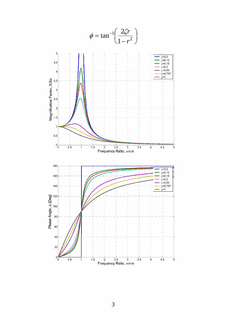
where M is the magnification factor (amplitude ratio) and

3

2

1

1

2tan

r

r

4

See figure 3.11

The total response of the system is the sum of the

homogeneous solution plus the particular solution or:

)cos()cos()()()( 0

tXteXtxtxtx od

tph

n

Note that the homogeneous solution xh(t) dies out with time,

and the steady-state solution prevails as long as the forcing

function is present.

To solve this, you find xp(0) and vp(0) and then find X0 and 0

such that the true initial conditions match x(0) and v(0).

5

Complex Analysis

Using the fact that the complex exponential is periodic, we

can look at the real component of tieFkxxcxm

0

we can assume a solution of the form:

( )i t

px t Xe

This leads to the equation:

2

0

i t i tm c i k Xe F e

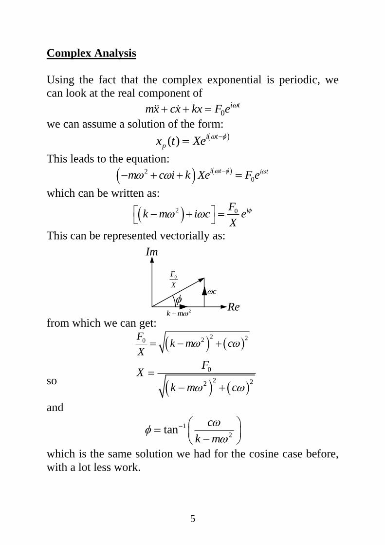
which can be written as:

2 0 iFk m i c e

X

This can be represented vectorially as:

from which we can get:

2 220F

k m cX

so

0

2 22

FX

k m c

and

1

2tan

c

k m

which is the same solution we had for the cosine case before,

with a lot less work.

0F

X

Re

Im

c

2k m

6

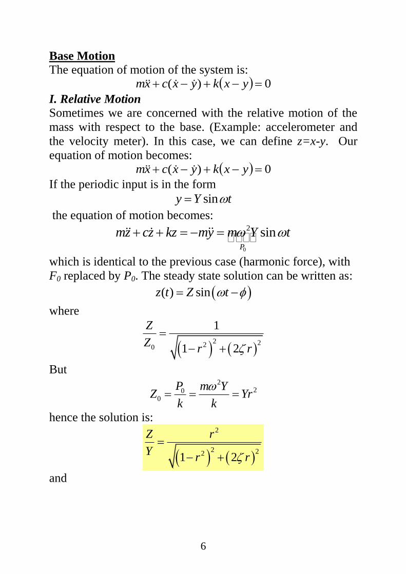
Base Motion

The equation of motion of the system is: 0)( yxkyxcxm

I. Relative Motion

Sometimes we are concerned with the relative motion of the

mass with respect to the base. (Example: accelerometer and

the velocity meter). In this case, we can define z=x-y. Our

equation of motion becomes: 0)( yxkyxcxm

If the periodic input is in the form

siny Y t

the equation of motion becomes:

0

2 sinP

mz cz kz my m Y t

which is identical to the previous case (harmonic force), with

F0 replaced by P0. The steady state solution can be written as:

( ) sinz t Z t

where

2 220

1

1 2

Z

Zr r

But 2

200

P m YZ Yr

k k

hence the solution is:

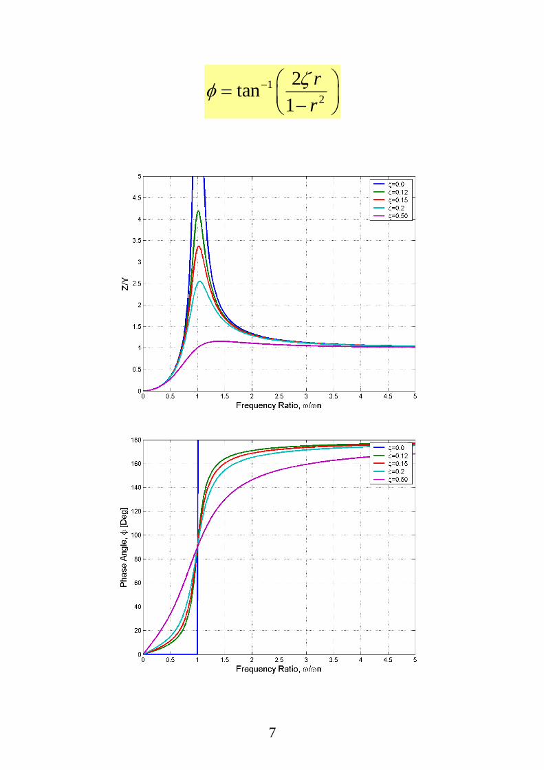
2

2 221 2

Z r

Yr r

and

7

1

2

2tan

1

r

r

8

Application: vibration measuring instruments

For negligible damping ( 1 ), we have 2

21

Z r

Y r

22

2Case 1: 1

n

r Z Yr Y

At “low” frequencies, Z is proportional to 2Y, i.e.

proportional to acceleration. In this range the accelerometer

works. It must have a high n such that n is small .

Case 2: 1r Z Y

At “high” frequencies, the ratio between Z and Y is one, i.e. Z

is equal to the displacement. In this range the vibrometer

works. It must have a low n such that n is high.

9

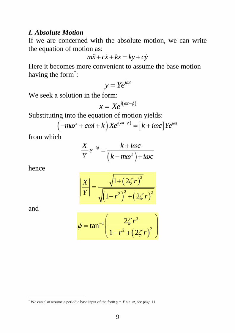
I. Absolute Motion

If we are concerned with the absolute motion, we can write

the equation of motion as:

mx cx kx ky cy

Here it becomes more convenient to assume the base motion

having the form*: i ty Ye

We seek a solution in the form: i t

x Xe

Substituting into the equation of motion yields:

2 i t i tm c i k Xe k i c Ye

from which

2

iX k i ce

Y k m i c

hence

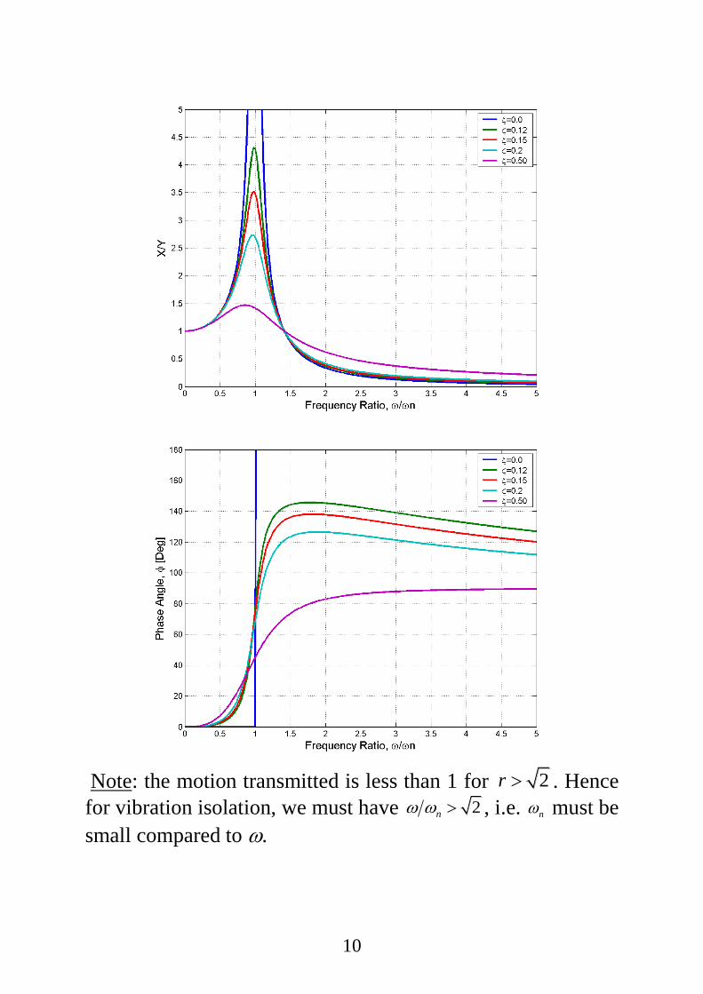
2

2 22

1 2

1 2

rX

Yr r

and

31

22

2tan

1 2

r

r r

* We can also assume a periodic base input of the form y = Y sin wt, see page 11.

10

Note: the motion transmitted is less than 1 for 2r . Hence

for vibration isolation, we must have 2n , i.e. n must be

small compared to .

11

The above solution can also be obtained if we assume a

periodic input of tYy sin

the equation of motion can be written as

sin cos

sin

mx cx kx kY t c Y t

mx cx kx A t

where

22 1, tan

cA Y k c

k

(see page 2)

But the above equation is in the same format now as the

forced vibration one, with an amplitude of A instead of F0

and an additional phase . So we can find (see page 2)

22

1 12

2 2 2

1

1 2

sin sin

tan

Y k cx X t t

k m c

c

k m

We can write the ratio of the amplitudes as

222

2 2 22 22

1 2

1 2

rk cX

Y k m c r r

using the same definition for and r as before, we can also

write the total solution as

tXtxp sin)(

where

22

31

22

31

141

2tantan

r

r

cmkk

mc

which is the same solution obtained using complex analysis.

12

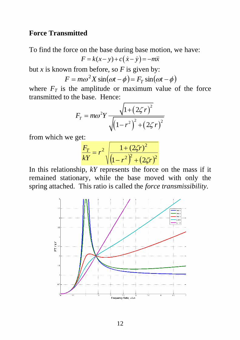
Force Transmitted

To find the force on the base during base motion, we have:

( )F k x y c x y mx

but x is known from before, so F is given by:

tFtXmF T sinsin2

where FT is the amplitude or maximum value of the force

transmitted to the base. Hence:

2

2

2 22

1 2

1 2T

rF m Y

r r

from which we get:

222

22

21

)2(1

rr

rr

kY

FT

In this relationship, kY represents the force on the mass if it

remained stationary, while the base moved with only the

spring attached. This ratio is called the force transmissibility.

13

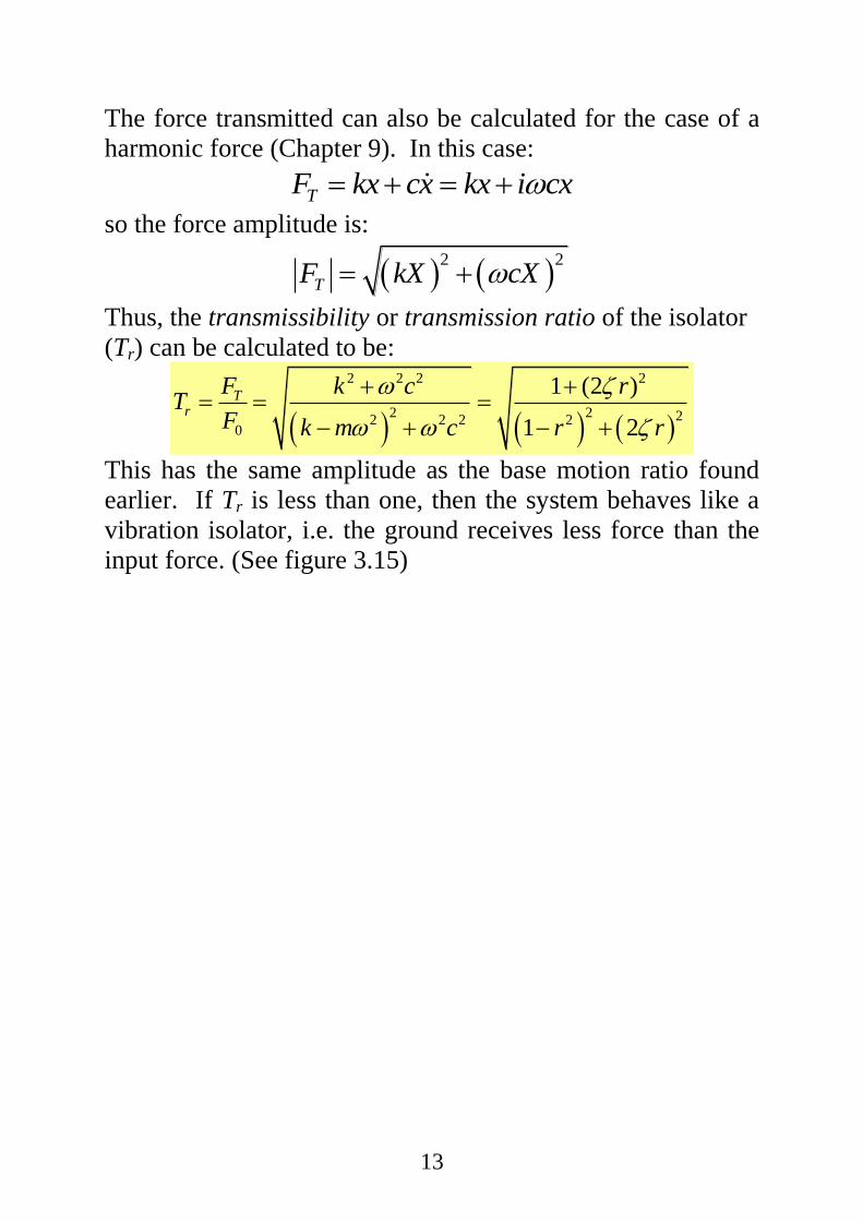
The force transmitted can also be calculated for the case of a

harmonic force (Chapter 9). In this case:

TF kx cx kx i cx

so the force amplitude is:

2 2

TF kX cX

Thus, the transmissibility or transmission ratio of the isolator

(Tr) can be calculated to be:

2 2 2 2

2 2 22 2 2 20

1 (2 )

1 2

Tr

F k c rT

F k m c r r

This has the same amplitude as the base motion ratio found

earlier. If Tr is less than one, then the system behaves like a

vibration isolator, i.e. the ground receives less force than the

input force. (See figure 3.15)

14

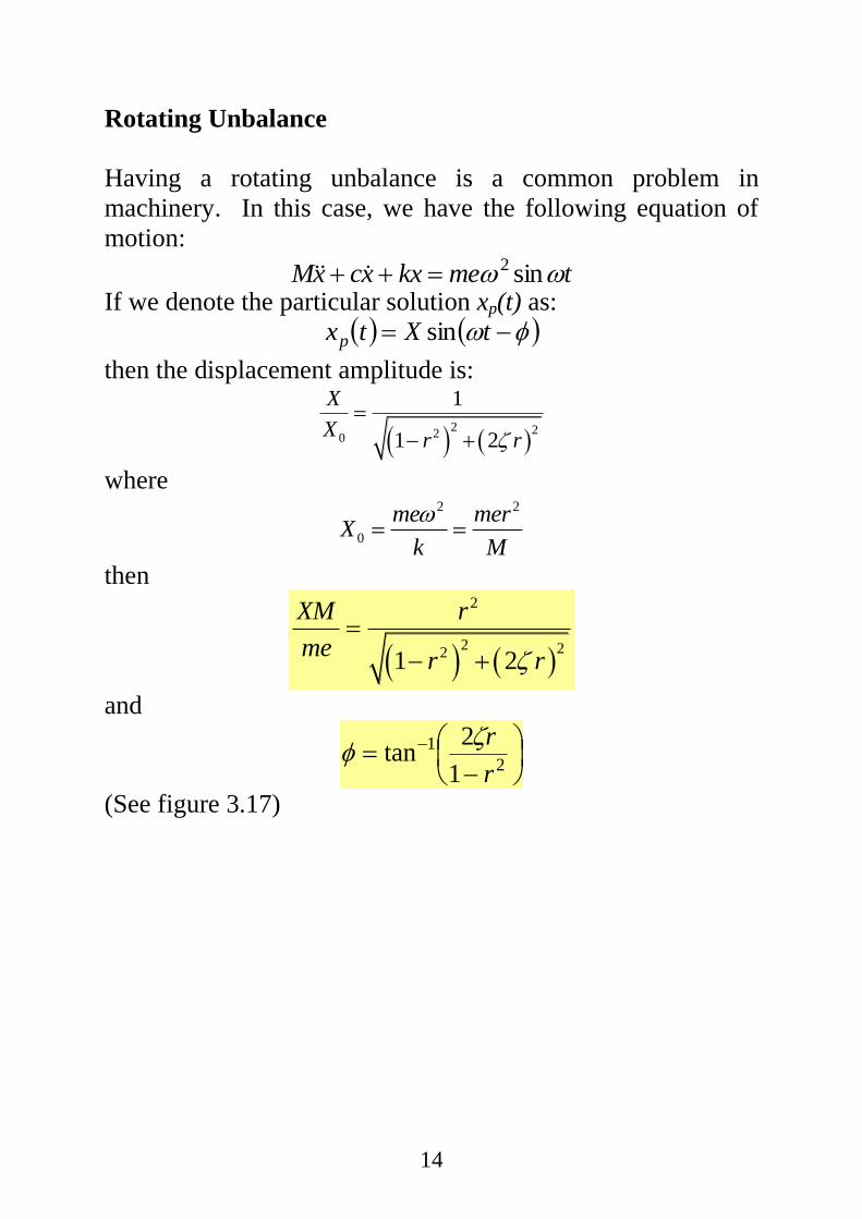
Rotating Unbalance

Having a rotating unbalance is a common problem in

machinery. In this case, we have the following equation of

motion:

tmekxxcxM sin2 If we denote the particular solution xp(t) as:

tXtxp sin

then the displacement amplitude is:

2 220

1

1 2

X

Xr r

where 2 2

0

me merX

k M

then

2

2 221 2

XM r

mer r

and

2

1

1

2tan

r

r

(See figure 3.17)

15

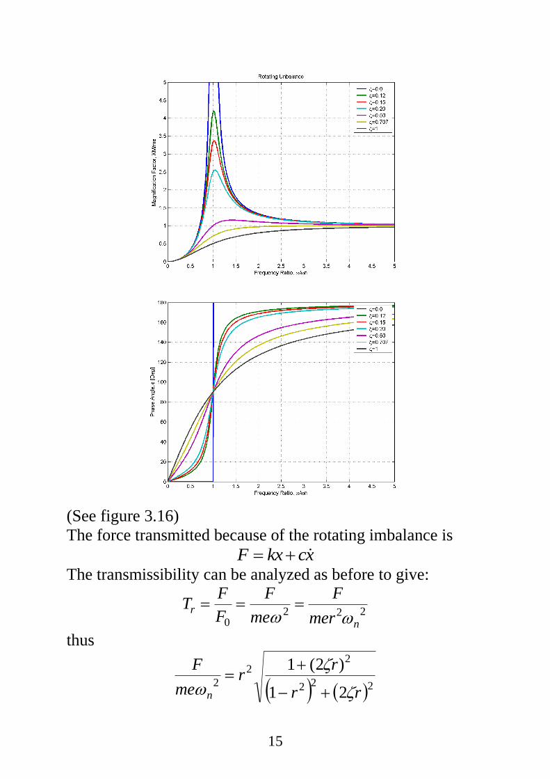
(See figure 3.16)

The force transmitted because of the rotating imbalance is

F kx cx The transmissibility can be analyzed as before to give:

2220 n

rmer

F

me

F

F

FT

thus

222

22

221

)2(1

rr

rr

me

F

n

16

Response under a general periodic force

If the forcing function is periodic, we can use the Fourier

series and the principle of superposition to get the response.

The Fourier series states that a periodic function can be

represented as a series of sines and cosines:

01 2 1 2

0

1

0

0

cos cos 2 ... sin sin 2 ...2

cos sin2

2cos , 0,1,2,

2sin , 1,2,3,

j j

j

T

j

T

j

aF t a t a t b t b t

aa j t b j t

a F t j t dt jT

b F t j t dt jT

where 2T is the period. Now the equation of motion

can be written as:

0

1

cos sin2

j j

j

amx cx kx F t a j t b j t

Using the principle of superposition, the steady-sate solution

of this equation is the sum of the steady-state solutions of:

tjbkxxcxm

tjakxxcxm

akxxcxm

j

j

sin

cos

2

0

The particular solution of the 1st equation is:

0

2p

ax t

k

17

The particular solutions of the 2nd and 3rd equations are:

2 22 2

2 22 2

1

2 2

cos

1 2

sin

1 2

2tan

1

j

p j

j

p j

j

n

a

kx t j t

j r jr

b

kx t j t

j r jr

jr

j r

r

Then add up all the sums to get the complete steady-state

solution as:

2 22 22 2 2 21 1

cos sin2

1 2 1 2

j j

op j j

j j

a ba k kx t j t j tk

j r jr j r jr

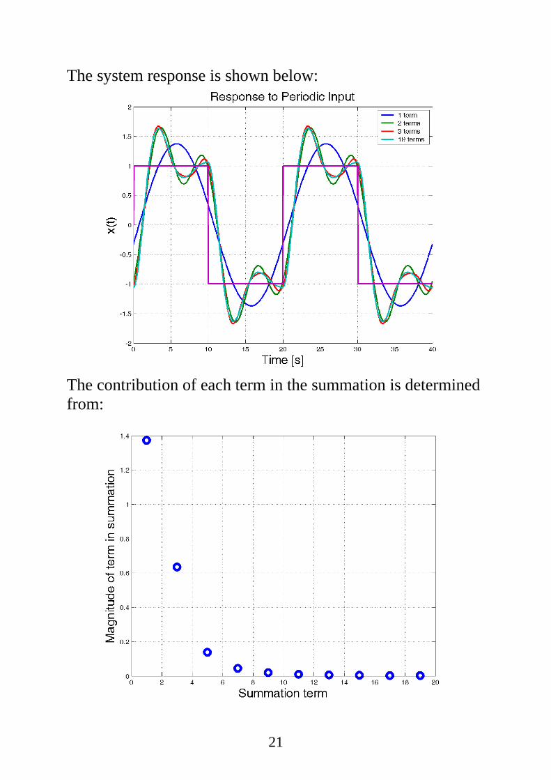
Observe that if nj , the amplitude will be significantly

large, especially for small j and . Further, as j becomes large,

the amplitude becomes smaller and the corresponding terms

tend to zero. How many terms do you need to include?

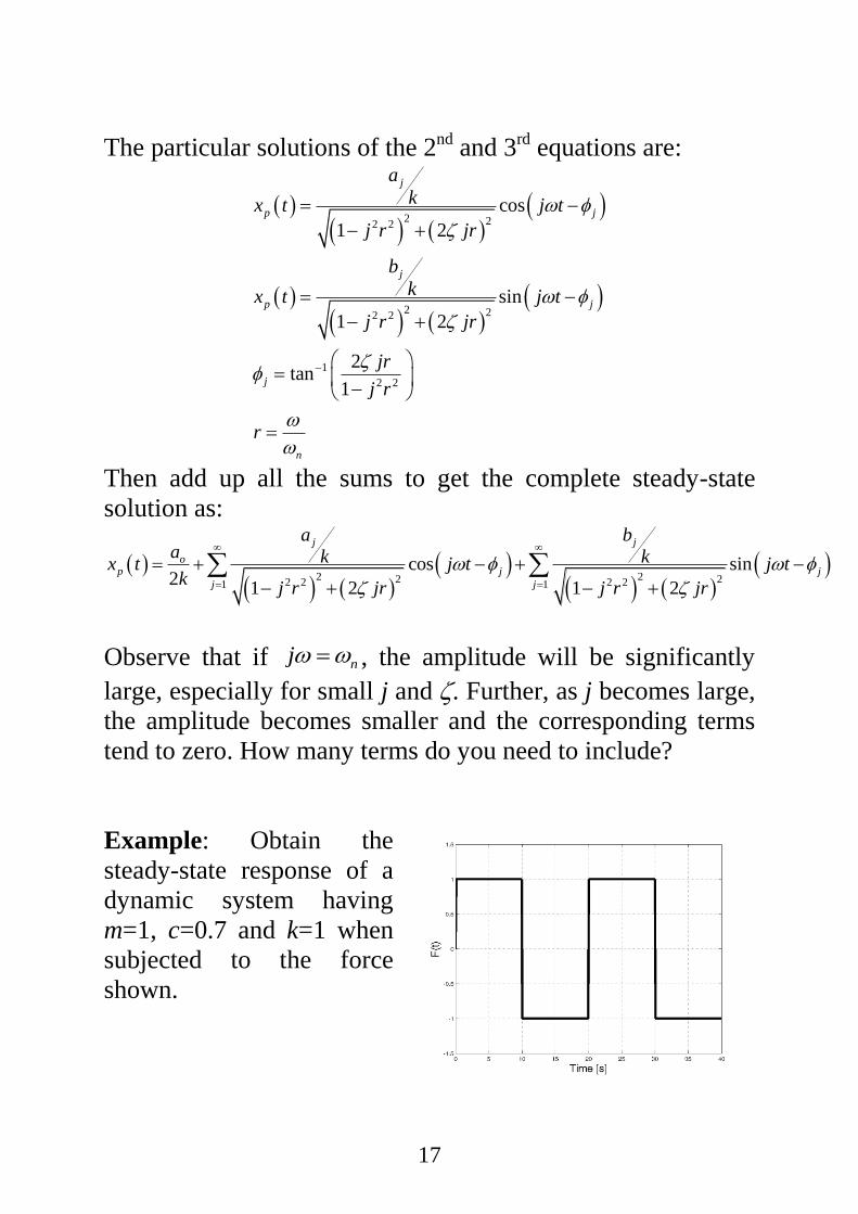
Example: Obtain the

steady-state response of a

dynamic system having

m=1, c=0.7 and k=1 when

subjected to the force

shown.

18

Solution: here we have:

20 , 2 2 20 10T T

and the forcing function is given by: ( ) 1 0 10

( ) 1 10 20

F t t

F t t

The Fourier series of the forcing function is given by:

01 2 1 2cos cos 2 ... sin sin 2 ...

2

aF t a t a t b t b t

To get the constants, we have:

10 20

00 0 10

2 20.1 10 20 10 0

20

T

a F t dt dt dtT

0

10 20

0 10

10 20

0 10

2cos

2cos cos

20 10 10

10 100.1 sin sin 0

10 10

T

ja F t j t dtT

j t dt j t dt

j t j tj j

i.e. all cosine terms vanish

0

10 20

0 10

10 20

0 10

2sin

2sin sin

20 10 10

10 100.1 cos cos

10 10

10 100.1 cos 1 cos 2 cos

T

jb F t j t dtT

j t dt j t dt

j t j tj j

j j jj j

19

If j is odd,

10 10 4

0.1 2 2jbj j j

If j is even,

10 10

0.1 0 0 0jbj j

i.e. all even terms vanish.

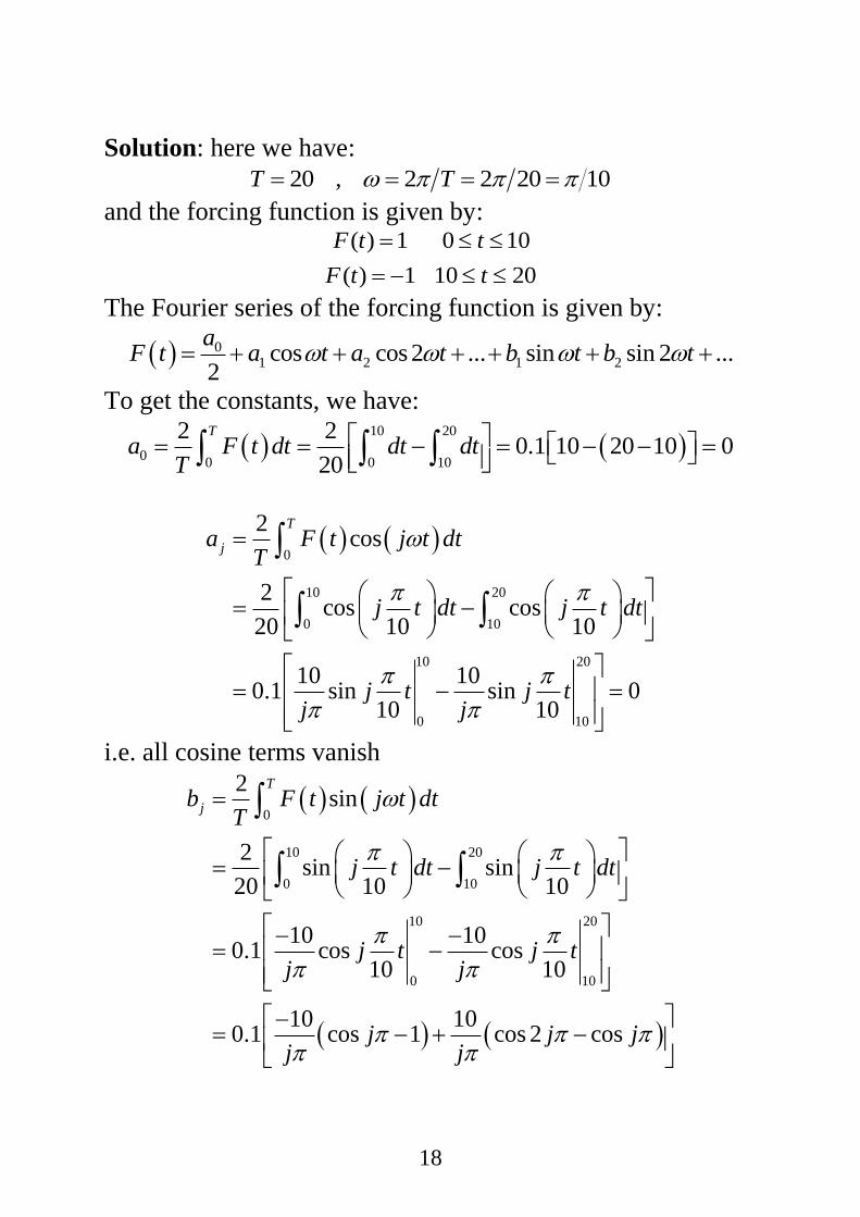
In this way, the force can be represented by a Fourier series

as:

1 1 3 3 5 5

1

1

( ) sin sin sin sin , 1,3,5,7,

4 4 3 4 5 4sin sin sin sin , 1,3,5,7,

10 3 10 5 10 10

j

j

j

F t b t b t b t b j t j

t t t j t jj

or graphically as:

20

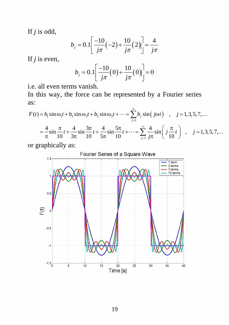
% *********************************************************** % Periodic response of a dynamic system to a square input waveform % *********************************************************** clear; close all; m=1; c=0.7; k=1; % Parameters wn=sqrt(k/m); zi=c/wn/2; w=pi/10; t=linspace(0,40,500); x=zeros(size(t)); r=w/wn; for jj=1:2:19 a(jj)=4/pi/jj; X(jj)=a(jj)/k/sqrt((1-jj^2*r^2)^2+(2*zi*jj*r)^2); % term in summation phi(jj)=atan2(2*zi*jj*r,1-jj*jj*r*r); x(jj+2,:)=x(jj,:)+X(jj)*sin(w*jj*t-phi(jj)); end u=sign(sin(w*t)); figure(1) plot(t,x([3 5 7 21],:),t,sign(sin(w*t)),'linewidth',2);grid legend('1 term','2 terms','3 terms','19 terms') xlabel('Time [s]','fontsize',18);ylabel('x(t)','fontsize',18) title('Response to Periodic Input','fontsize',18); figure(2) plot(1:2:19,X(1:2:19),'o','markersize',10,'linewidth',4);grid ylabel('Magnitude of term in summation','fontsize',18) xlabel('Summation term','fontsize',18)

21

The system response is shown below:

The contribution of each term in the summation is determined

from:

22

Response to an impulse

From ENGR 214, the principle of impulse and momentum

states that impulse equals change in momentum:

𝐼𝑚𝑝𝑢𝑙𝑠𝑒 = 𝐹∆𝑡 = 𝑚(𝑣2 − 𝑣1)

or:

𝐹 = 𝐹𝑑𝑡 = 𝑚𝑥 2 − 𝑚𝑥 1

𝑡+∆𝑡

𝑡

A unit impulse is defined as:

𝑓 = lim∆𝑡→0

𝐹𝑑𝑡 = 1𝑡+∆𝑡

𝑡

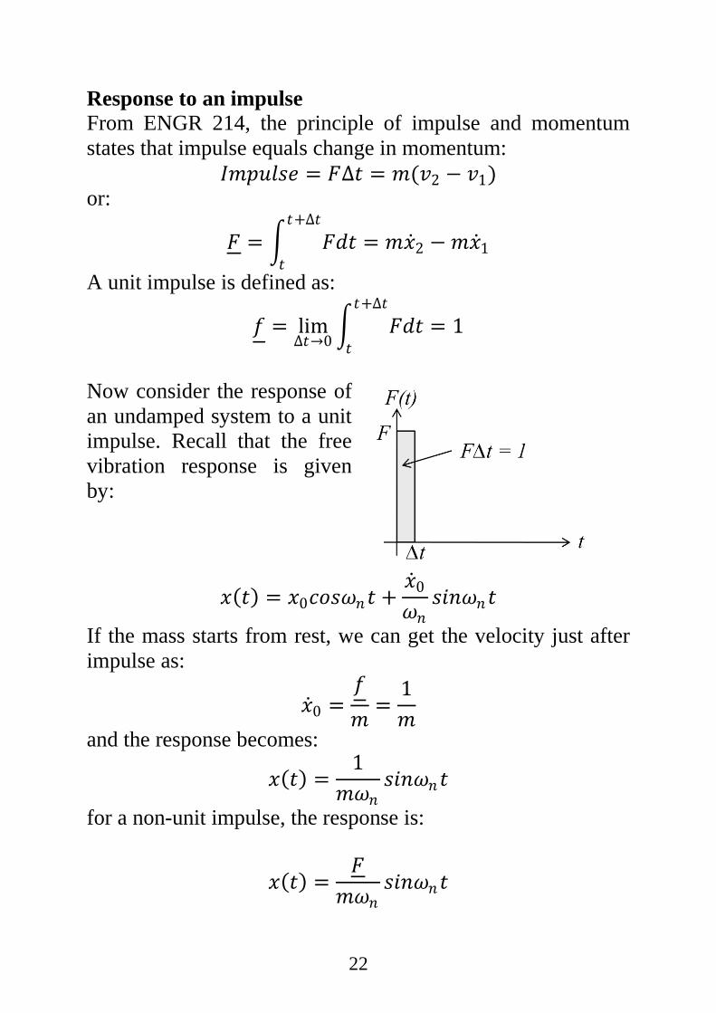
Now consider the response of

an undamped system to a unit

impulse. Recall that the free

vibration response is given

by:

𝑥 𝑡 = 𝑥0𝑐𝑜𝑠𝜔𝑛𝑡 +𝑥 0𝜔𝑛

𝑠𝑖𝑛𝜔𝑛𝑡

If the mass starts from rest, we can get the velocity just after

impulse as:

𝑥 0 =𝑓

𝑚=

1

𝑚

and the response becomes:

𝑥 𝑡 =1

𝑚𝜔𝑛𝑠𝑖𝑛𝜔𝑛𝑡

for a non-unit impulse, the response is:

𝑥 𝑡 =𝐹

𝑚𝜔𝑛𝑠𝑖𝑛𝜔𝑛𝑡

23

For an underdamped system, recall that the free response was

gven by: (see page 142)

𝑥 𝑡 = 𝑒−𝜁𝜔𝑛 𝑡 𝑥0𝑐𝑜𝑠𝜔𝑑𝑡 +𝑥 0 + 𝜁𝜔𝑛𝑥0

𝜔𝑑𝑠𝑖𝑛𝜔𝑑𝑡

For a unit impulse, the response for zero initial conditions is:

𝑥 𝑡 =𝑒−𝜁𝜔𝑛 𝑡

𝑚𝜔𝑑𝑠𝑖𝑛𝜔𝑑𝑡 = 𝑔(𝑡)

where 𝑔(𝑡) is known as the impulse response function. For a

non-unit impulse, the response is:

𝑥 𝑡 =𝐹𝑒−𝜁𝜔𝑛 𝑡

𝑚𝜔𝑑𝑠𝑖𝑛𝜔𝑑𝑡 = 𝐹𝑔(𝑡)

If the impulse occurs at a delayed time 𝑡 = 𝜏, then

𝑥 𝑡 =𝐹𝑒−𝜁𝜔𝑛 𝑡−𝜏

𝑚𝜔𝑑𝑠𝑖𝑛𝜔𝑑 𝑡 − 𝜏 = 𝐹𝑔(𝑡 − 𝜏)

If two impulses occur at two different times, then their

responses will superimpose.

Example: For a system having 𝑚 = 1 kg; 𝑐 = 0.5 kg/s; 𝑘 =4 N/m; F = 2 Ns obtain the response when two impulses are

applied 5 seconds apart.

Solution: here we have 𝜔𝑛 = 2rad

s, ζ = 0.125, 𝜔𝑑 =

1.984rad

s so the solutions become:

𝑥1 𝑡 =2𝑒−0.25𝑡

1.984sin 1.984𝑡 𝑡 > 0

𝑥2 𝑡 =2𝑒−0.25 𝑡−𝜏

1.984sin 1.984 𝑡 − 𝜏 𝑡 > 5

And the total response is:

24

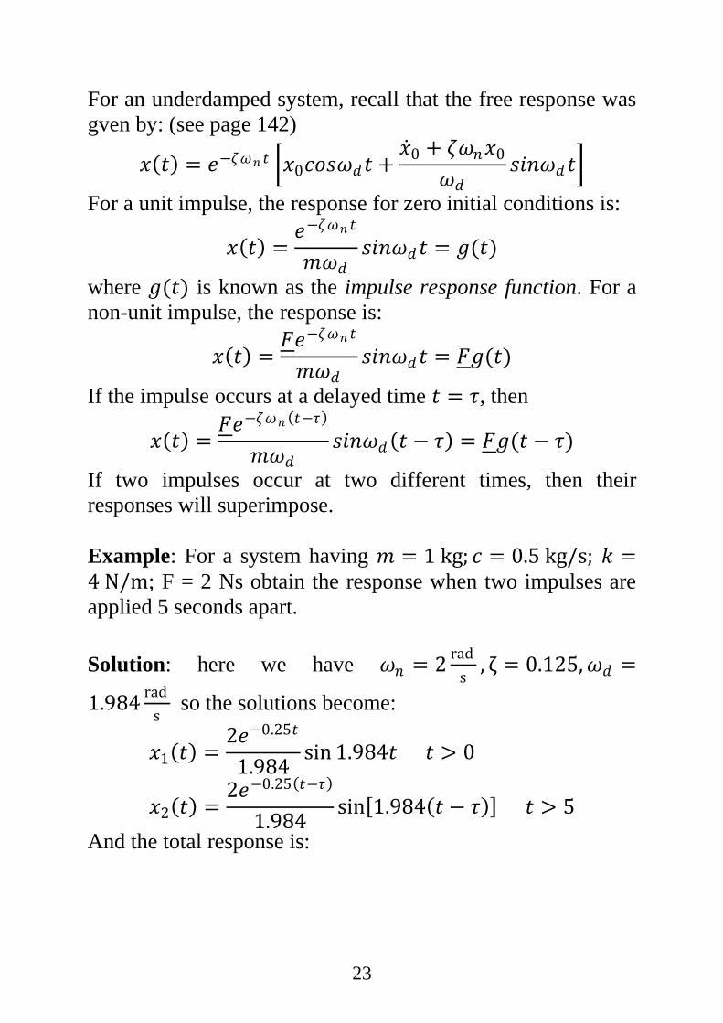
𝑥 𝑡

=

2𝑒−0.25𝑡

1.984sin 1.984𝑡 0 < 𝑡 < 5

2𝑒−0.25𝑡

1.984sin 1.984𝑡 +

2𝑒−0.25 𝑡−𝜏

1.984sin 1.984 𝑡 − 𝜏 5 < 𝑡 < 20

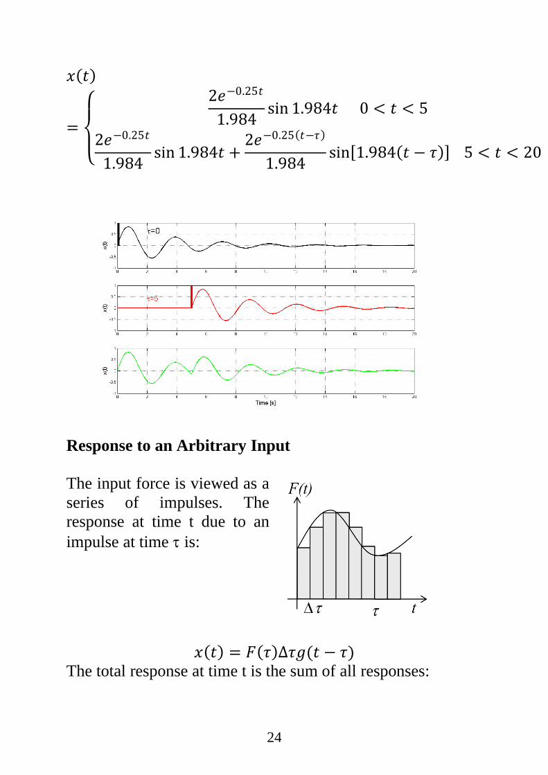
Response to an Arbitrary Input

The input force is viewed as a

series of impulses. The

response at time t due to an

impulse at time is:

𝑥 𝑡 = 𝐹 𝜏 ∆𝜏𝑔(𝑡 − 𝜏)

The total response at time t is the sum of all responses:

25

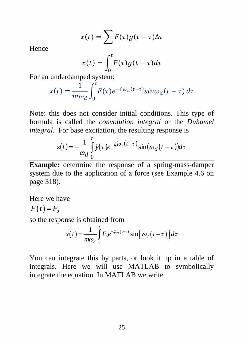
𝑥 𝑡 = 𝐹 𝜏 𝑔 𝑡 − 𝜏 ∆𝜏

Hence

𝑥 𝑡 = 𝐹 𝜏 𝑔 𝑡 − 𝜏 𝑑𝜏𝑡

0

For an underdamped system:

𝑥 𝑡 =1

𝑚𝜔𝑑 𝐹 𝜏 𝑒−𝜁𝜔𝑛 𝑡−𝜏 𝑠𝑖𝑛𝜔𝑑 𝑡 − 𝜏

𝑡

0

𝑑𝜏

Note: this does not consider initial conditions. This type of

formula is called the convolution integral or the Duhamel

integral. For base excitation, the resulting response is

t

dt

d

dteytz n

0

sin1

Example: determine the response of a spring-mass-damper

system due to the application of a force (see Example 4.6 on

page 318).

Here we have

0F t F

so the response is obtained from

0

0

1sinn

tt

d

d

x t F e t dm

You can integrate this by parts, or look it up in a table of

integrals. Here we will use MATLAB to symbolically

integrate the equation. In MATLAB we write

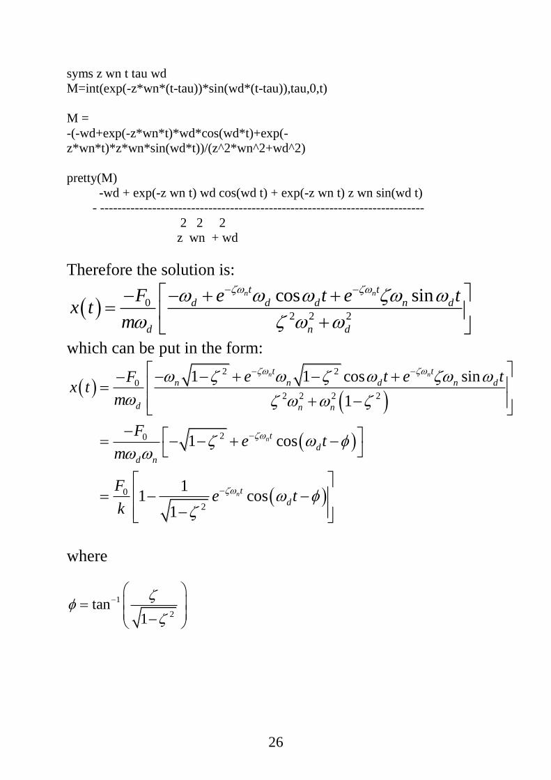
26

syms z wn t tau wd

M=int(exp(-z*wn*(t-tau))*sin(wd*(t-tau)),tau,0,t)

M =

-(-wd+exp(-z*wn*t)*wd*cos(wd*t)+exp(-

z*wn*t)*z*wn*sin(wd*t))/(z^2*wn^2+wd^2)

pretty(M)

-wd + exp(-z wn t) wd cos(wd t) + exp(-z wn t) z wn sin(wd t)

- ---------------------------------------------------------------------------

2 2 2

z wn + wd

Therefore the solution is:

0

2 2 2

cos sinn nt t

d d d n d

d n d

F e t e tx t

m

which can be put in the form:

2 2

0

2 2 2 2

20

0

2

1 1 cos sin

1

1 cos

11 cos

1

n n

n

n

t t

n n d n d

d n n

t

d

d n

t

d

e t e tFx t

m

Fe t

m

Fe t

k

where

1

2tan

1

27

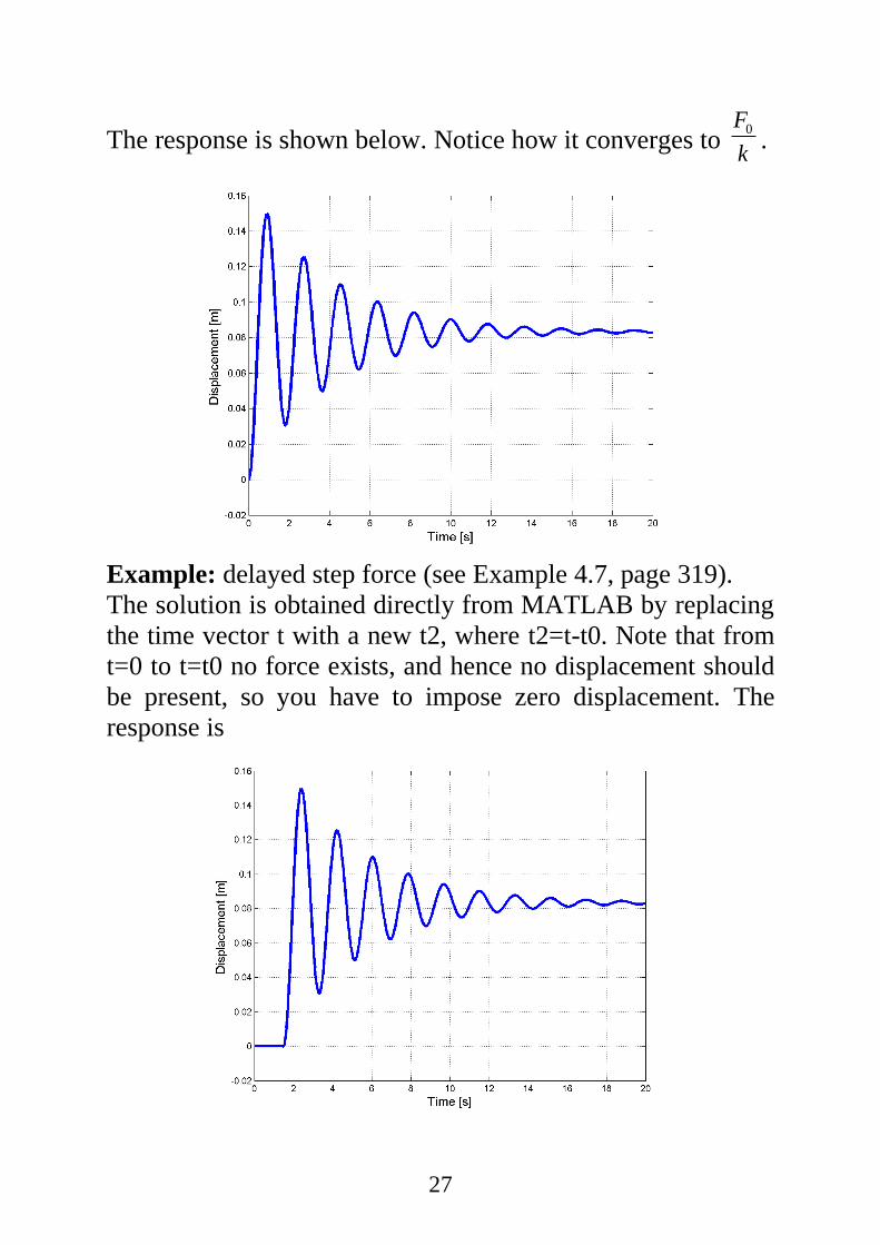
The response is shown below. Notice how it converges to 0F

k.

Example: delayed step force (see Example 4.7, page 319).

The solution is obtained directly from MATLAB by replacing

the time vector t with a new t2, where t2=t-t0. Note that from

t=0 to t=t0 no force exists, and hence no displacement should

be present, so you have to impose zero displacement. The

response is

28

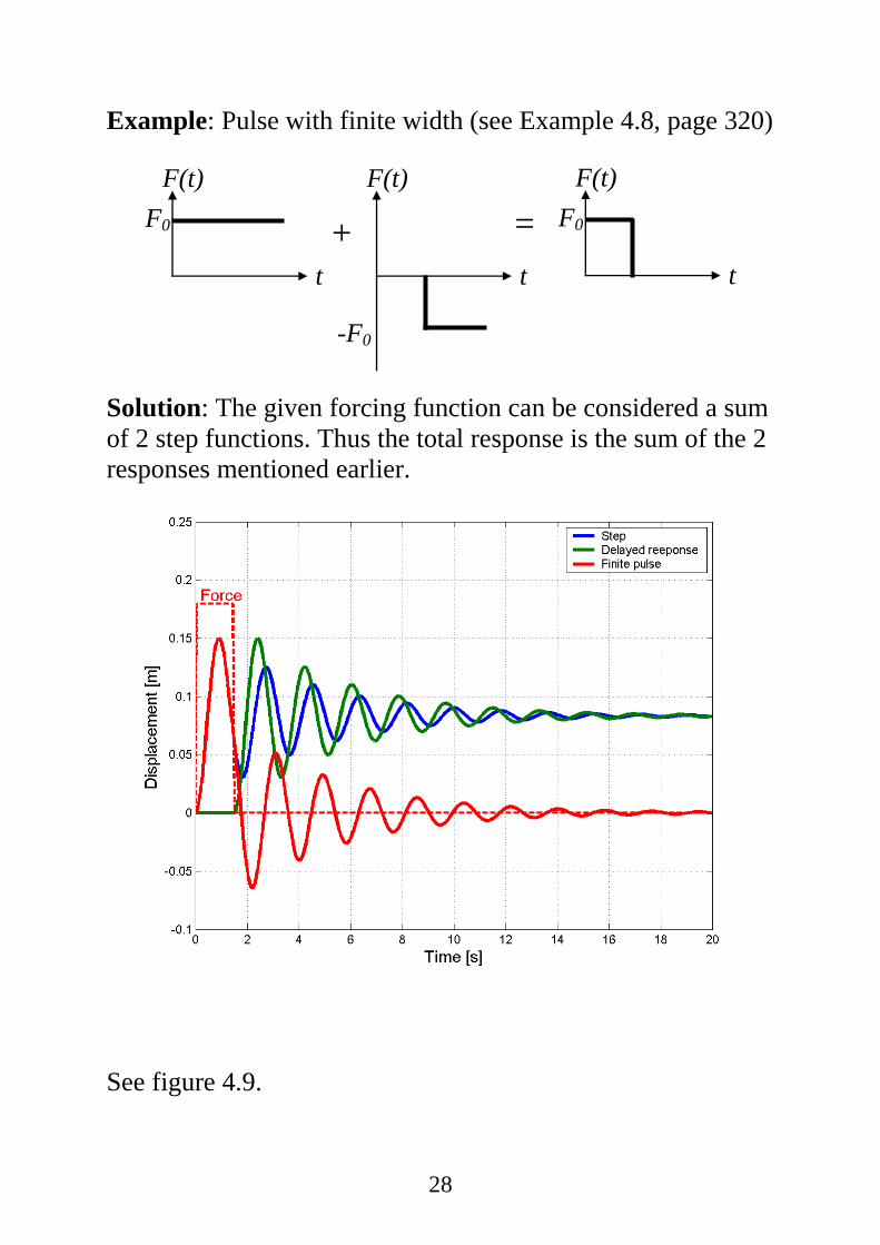
Example: Pulse with finite width (see Example 4.8, page 320)

Solution: The given forcing function can be considered a sum

of 2 step functions. Thus the total response is the sum of the 2

responses mentioned earlier.

See figure 4.9.

F(t)

t

F0

F(t)

t

-F0

F(t)

t

F0 + =

29

If there is no damping (c=0) some interesting things can

happen

2

00

1

)cos()cos(sin)cos()(

n

nstn

n

n

ttt

xtxtx

As the forced frequency approaches the natural frequency

(n)

tttt

d

d

ttd

d

tt

n

n

n

n

n

n

nn

sin2

2

sinlim

1

)cos()cos(

lim

1

)cos()cos(lim

2

22

so

tt

tx

txtx stn

n

n

sin2

sin)cos()( 00

See Fig 3.6

If the frequencies are close (n) then a phenomena called

beating occurs. Assuming zero initial conditions

ttm

F

tttx

nn

n

n

nst

2sin

2sin2

1

)cos()cos()(

220

2

Using the following notation

422 22 nnn

30

then

tttx st

sinsin

2)(

This will be a sin wave with a slowly varying sinusoidal

magnitude.

Forced vibration with Coulomb Damping

For the system

tFkxNxm cos0

the solution is

2

201

2

2

2

2

00

1

4

tan

1

41

cos

nn

p

F

N

F

N

k

FX

tXtx

which is valid for F0>>N

Forced vibration with Hysteretic Damping

For the system

tFkxxbk

xm

cos0

the solution is

2

2

1

2

2

2

2

0

1

tan

1

cos

nn

p

k

F

X

tXtx

See figure 3.24

31