Response to Harmonic Excitation

Part 2: Damped Systems

Part 1 covered the response of a single degree of freedom system to harmonic excitation

without considering the effects of damping. However, almost every real world system that is

analyzed from a vibrations point of view has some source of energy dissipation or damping.

This module will expand on Part 1 and discuss the response of such a system to harmonic

excitations with the effects of viscous damping included.

Harmonic Excitation of Damped Systems

Fig 1: Spring-mass-damper with external force

Consider a simple spring-mass system with damping being driven by a force of the

form on a frictionless surface. Here is the magnitude of the applied

force and is the angular frequency of the applied force. The sum of the forces in the y-

direction is 0, resulting in no motion in that direction. In the x-direction, summing the forces

on the mass yields

... Eq. (1)

Dividing through by gives

... Eq. (2)

where, as a reminder,

, is the natural frequency of the system and

is the damping ratio. There are many ways of finding a solution to this type of a

differential equation (Laplace transform approach, geometric method, method of

undetermined coefficients, etc.). Here, the method of undetermined coefficients will be used

by assuming the particular solution has the form shown in Eq. (3). It is known, from

observation and from the study of differential equations, that the forced response of a

damped system has the same frequency as the driving force but with a different amplitude

and phase. Therefore, the particular solution of Eq. (2) is assumed to be of the form

... Eq. (3)

To simplify the computations, this can be written as

... Eq. (4)

where and such that and . Taking

derivatives of Eq. (4) we get

... Eq. (5)

and

... Eq. (6)

Substituting these two equations into Eq. (2) gives

... Eq. (7)

This can be further simplified to

.. Eq. (8)

This equation must be valid for all values of . When , Eq. (9) simplifies to

... Eq. (9)

and when , Eq. (9) simplifies to

... Eq. (10)

Solving these two equations, gives

... Eq. (11)

and

... Eq. (12)

Substituting Eqs. (11) and (12) back into Eq. (4) and rewriting it in the form of Eq. (3), gives

... Eq. (13)

This is the equation for the particular solution. For the total solution, we need to add the

homogeneous solution to this. For an underdamped system, we add Eq. (12) from the Free

Response Part 2 module to get

... Eq. (14)

where, using the initial conditions and , the constant are given by

and

... Eqs. (15) to (18)

Eq. (14) is the total solution for an underdamped system. The total solutions for a critically

damped or overdamped system can be found using the same method of adding the

homogeneous solution to the particular solution and using the initial conditions to find the

constants.

From Eq. (14) you can see that for relatively large values of , the homogeneous part of the

total solution approaches zero (this also applies to critically damped and overdamped

systems because the homogeneous solutions for these two types of systems also decay

with time). This means that as time increases, the total solution approaches the particular

solution, which is also why the particular solution is also called the steady state response

and the homogeneous solution is called the transient response. The following plots show a

comparison of the total response and the steady-state response for a spring-mass system

with different damping coefficients (the initial conditions and other parameters are kept

constant: ).

Comparison for zeta=1.5Comparison for zeta=1.5

Comparison for zeta=0.05Comparison for zeta=0.05

Comparison for zeta=5Comparison for zeta=5

For the following plot, the damping coefficient, the spring constant and the initial conditions

can be adjusted using the gauges to see the effect on the total response. The rest of the

parameters of the system are the same as for the above plots (

).

As can be seen from the plots, the total response and the steady-state response merge

after some time. In many cases, depending on the system and the purpose of the analysis,

the transient response may die out very quickly and may be ignored. These plots also show

that the amplitude of the steady-state vibrations depend on the damping coefficient.

From Eq. (18), it is clear that the amplitude of the steady state vibrations also depends on

the driving frequency. By defining another ratio, , called the frequency ratio, Eq. (18)

can be rewritten as the following equation for the normalized amplitude of the steady-state

response.

... Eq. (19)

This equation is plotted vs. the frequency ratio for different values of :

Normalized amplitude vs. frequency ratioNormalized amplitude vs. frequency ratio

From this plot, it can be seen that for systems with low damping coefficients, the amplitude

is maximum close to (when the driving frequency is equal to the natural frequency).

Also, it is important to note that, as the damping increases, the frequency for which the

maximum amplitude is obtained shifts away from the natural frequency until there is no

peak. The maximum amplitude is obtained when if and there is

no peak if This information can be very important from a design point of view.

Similar to Eq. (19) the following equation shows the phase of the steady-state response as

a function of the frequency ratio .

... Eq. (20)

The following plot shows the phase vs. the frequency ratio.

Amplitude vs. frequency ratioAmplitude vs. frequency ratio

This plot shows that as the driving frequency increases, the phase difference between the

steady-state response and the driving force increases from 0 to Pi and is equal to Pi/2 (90 )

at the natural frequency of the system.

Examples with MapleSim

Example 1: Spring-mass oscillator

Compute the steady-state response of a spring-mass system with damping for the values

given below and plot the response for 10 seconds.

Table 1: Example 1 parameter values

Parameter

Value

1000 N/m

100 N$s/m

10 kg

100 N

8.16 rad/s

0.01 m

0.01 m/s

Analytical Solution

Data:

[N/m]

[kg]

[N$s/m]

[N]

[rad/s]

[m]

(2.1.1.1)(2.1.1.1)

[m/s]

Solution:

The natural frequency is

= 10

and the damping ratio is

= 12

Using Eq. (13) the steady-state response is given by

where

The expression for the steady-state response, , is

MapleSim Simulation

Step1: Insert Components

Drag the following components into the workspace:

Table 2: Components and locations

Component Location

1-D Mechanica

l > Translation

al > Common

1-D Mechanica

l > Translation

al > Common

1-D Mechanica

l > Translation

al > Common

1. 1.

2. 2.

1-D Mechanica

l > Translation

al > Common

Signal Blocks > Common

Step 2: Connect the components

Connect the components as shown in the following diagram.

Fig. 2: Component diagram

Step 3: Set parameters and initial conditions

Click the Translational Spring Damper component, enter 1000 N/m for the

spring constant ( ), and enter 100 N$s/m for the damping constant ( ).Click the Mass component and enter 10 kg for the mass ( ), 0.01 m/s for the

initial velocity ( ) and 0.01 m for the initial position ( ). Select the check marks

that enforce these initial condition.

2. 2.

3. 3.

1. 1.

Click the Sine Source component and enter 100 for the amplitude, 8.16 rad/s for

the frequency ( ) and Pi/2 for the phase ( ) [since we are assuming that the

excitation is a cosine function].

Step 4: Run the Simulation

Attach a Probe to the Mass component as shown in Fig. 2. Click this Probe and

select Length in the Inspector tab. This shows the position of the mass as a

function of time.

Click Run Simulation ( ).

Example 2: Spring-Pendulum

Problem Statement: A component of a machine

is modeled as a pendulum connected to a spring

(as shown in Fig. 3). This component is driven by

a motor that applies a sinusoidal moment

Nm about the axis of rotation.

Derive the equation of motion and find the natural

frequency of the system. The mass of the

pendulum is 2kg, the length of the pendulum is

0.5m, the stiffness of the spring is 20 N/m and the

damping coefficient is 20 N$s/m. Assume that the

rod of the pendulum has no mass. The initial

angular displacement is 0.175 rad (approx. 10 )

measured from the vertical and there is no initial

angular velocity.

a) Plot the total response and find the maximum

angular displacement of the pendulum.

b) Find the angular frequency of the applied

moment that would lead to steady state vibrations

of the maximum amplitude.

Fig. 3: Spring-pendulum example

3. 3.

Analytical Solution

Data:

[kg]

[m]

[N/m]

[N$s/m]

[m/s2]

[rad]

[rad/s]

[rad/s]

Solution:

Part a) Total response

Using the small angle approximation, we will assume that the spring stretches and

compresses in the horizontal direction only. Hence the force due to the spring can

be written as

and the force due to the damper can be written as

Taking the sum of the moments of force about the pivot gives

where is the moment of inertia of the pendulum. This equation can be rewritten as

3. 3.

or

:

Comparing this equation to the form of Eq. (2) and using Eq. (14), the total

response can be written as

where

=

= 0.1328885174

= 4.661477770

3. 3.

The following shows the plot of the total response for 10 seconds.

From this plot, it can be concluded that the maximum displacement is

approximately 0.29 rad at approximately 0.17 seconds.

Part b) Driving frequency for maximum amplitude steady-state vibrations

The amplitude of the steady-state oscillations is given by

where is the driving frequency. To find the value of for which the amplitude

will be maximum, this expression is differentiated with respect to and equated tozero.

(2.2.1.2.2)(2.2.1.2.2)

3. 3.

(2.2.1.2.1)(2.2.1.2.1)

solve for w__F

Ignoring and (does not make physical sense), we can

conclude that the amplitude of the steady state oscillations will be maximum when

the driving frequency is approximately 4.62 rad/s which is very close to the natural

frequency of 4.70 rad/s.

MapleSim Simulation

Constructing the model

Step1: Insert Components

Drag the following components into the workspace:

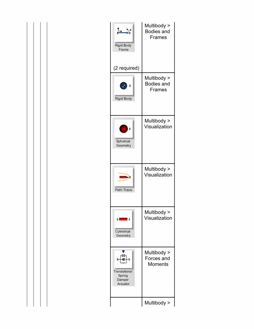
Table 3: Components and locations

Component Location

(2 required)

Multibody > Bodies and

Frames

Multibody > Joints and

Motions

3. 3.

(2 required)

Multibody > Bodies and

Frames

Multibody > Bodies and

Frames

Multibody > Visualization

Multibody > Visualization

Multibody > Visualization

Multibody > Forces and

Moments

Multibody >

3. 3.

Visualization

Multibody > Forces and

Moments

Signal Blocks > Common > Sine Source

Step 2: Connect the components

Connect the components as shown in the following diagram (the dashed boxes are

not part of the model, they have been drawn on top to help make it clear what the

different components are for).

1. 1.

3. 3.

2. 2.

1. 1.

3. 3.

2. 2.

Fig. 4: Component diagram

Step 3: Set up the Pendulum

Click the Revolute component and enter 0.175 rad for the initial angle ( ) and

select Strictly Enforce in the drop down menu for the initial conditions ( ).

The axis of rotation ( ) should be left as the default axis [0,0,1].

Enter [0,-0.25,0] for the x,y,z offset ( ) of both the Rigid Body Frames.

Enter 2 kg for the mass ( ) of the Rigid Body Frame.

Step 4: Set up the Spring

Click the Fixed Frame component connected to the TSDA (FF1 in the

diagram) and enter [-0.25,-0.25,0] for the x,y,z offset ( ).

Click the TSDA component, enter 20 N/m for the spring constant ( ) and

enter 20 N$s/m for the damping constant ( ). Also, enter 0.25 m for the

unstretched length ( ) to correspond to the location of the Fixed Frame.

Step 5: Set up the external sinusoidal moment (Motor)

1. 1.

1. 1.

2. 2.

2. 2.

1. 1.

3. 3.

3. 3.

2. 2.

Click the Sine Source component and enter 10 for the amplitude, 4*Pi rad/s

for the frequency ( ) and Pi/2 for the phase ( ) [the external force is a cosine

function].

Connect the output of the Sine Source component to the z input of the Applied World Moment component.

Step 6: Set up the visualization (Inserting the Visualization components is optional)

Click the Cylindrical Geometry component and enter a value around 0.01 m

for the radius.

Click the Spherical Geometry component and enter a value around 0.05 m

for the radius.

Click the Spring Geometry component, enter a number around 10 for the

number of windings, enter a value around 0.02 m for radius1 and enter a

value around 0.005 m for radius2.

Step 7: Run the Simulation

Click the Probe attached to the Revolute joint and select Angle to obtain a

plot of the angular position vs. time.

Click Run Simulation ( ).

Since the analytical solution makes a small angle approximation, there will be a very

slight variation in the results of this simulation and the results of the analytical method.

From the plot generated using the analytical approach, the maximum amplitude is

found to be approximately 0.29 rad. And, from the plot generated using the simulation,

the maximum amplitude is found to be approximately 0.28 rad.

The following image shows the plot obtained from the simulation that shows the angle

with respect to time.

3. 3.

1. 1.

Fig. 5: Simulation results - theta (rad) vs. t (s)

The following video shows the visualization of the simulation

Video Player

Video 1: Visualization of the spring-pendulum simulation with damping

3. 3.

1. 1.

Example 3: Wind turbine vibrations

Problem statement: The wind turbine described below has three rotor blades, one of

which has a moment of inertia which is 1 percent less than the moment of inertia of the

other two blades. Obtain a plot of the system response for a range of rotational speeds.

Description

The tower of a small wind turbine is a

hollow steel cylinder of height 10 m with

inner and outer diameters of 0.2 m and

0.15 m respectively. The density of the

steel is 7800 Kg/m3 and its modulus of

elasticity is approximately 2 x1011 N/m2.

The mass of the nacelle and its contents

(the generator and the drivetrain) is

approximately 500 kg. The wind turbine

has three rotor blades. Two of the blades

blade have a mass of 10 Kg and a mass

moment of inertia of approximately 20

kg/m2. One of the blades has a moment

of inertia which is 1% less than the other

blades. This unbalance may be due to

manufacturing defects, damage, wear,

etc.

Fig. 6: Wind turbine

MapleSim Model

In this example, we will create a simplified lumped mass model of a wind turbine to

1. 1.

3. 3.

study the vibrations due to unbalanced rotors.

The tower can be modeled as a cantilever beam with a tip mass subjected to a tip

force. Based on the Euler-Bernoulli beam theory the deflection at the tip of a

cantilever beam due to a tip force is

where is the tip force, is the length of the beam, is the modulus of elasticity of

the material and is the area moment of inertia of the beam. This equation can be

rewritten as

Therefore, the tower can be modeled as a spring with stiffness

In this case,

where is the outer diameter of the tower and is the inner diameter.

To simplify the model, it will be assumed that the tower behaves as a rod hinged at

the base. The mass moment of inertia of a rod about an axis passing through one end

is

1. 1.

3. 3.

so the mass of the tower will be included in the model as a point mass of mass

located at the tip of the tower. The mass of the tower can be calculated using the

following expression

where is the density of the steel and is the height of the tower. The mass of the

nacelle and its contents (the generator and the drivetrain) is approximately 500 kg.

This will also be modeled as a point mass at the tip of the tower. The wind turbine has

three rotor blades. Each blade has a mass of 10 Kg and a mass moment of inertia of

approximately 20 kg/m2. Each blade can be modeled as a point mass of 10 kg located

at a distance of m from the axis of rotation. To study the effect of the unbalanced

mass, the mass of one of the three blades will be set as 0.99$10 kg.

The following image shows the component diagram for the model.

Fig. 7: Wind turbine simulation component diagram

As can be seen from this diagram, a Ramp component is used to apply a linearly

increasing angular speed to the rotor. Also, CAD models for the rotor blades and the

rotor hub have been attached for a more interesting visualization.

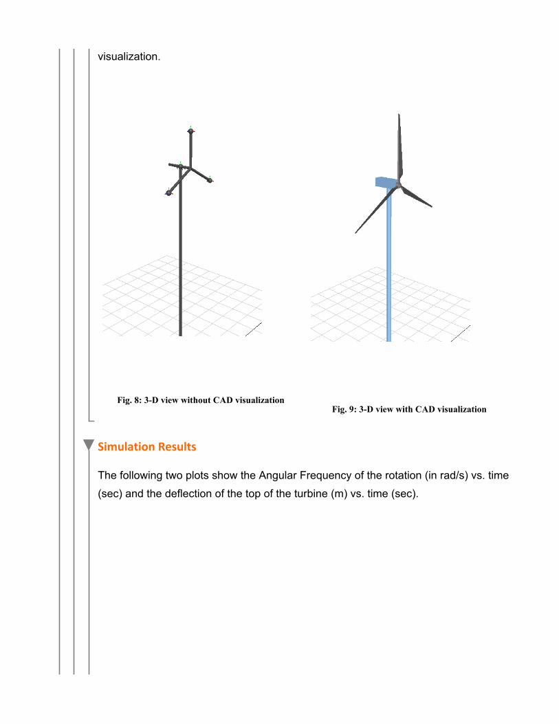
The following two images show the 3-D view of the simulation without and with

3. 3.

1. 1.

visualization.

Fig. 8: 3-D view without CAD visualization Fig. 9: 3-D view with CAD visualization

Simulation Results

The following two plots show the Angular Frequency of the rotation (in rad/s) vs. time

(sec) and the deflection of the top of the turbine (m) vs. time (sec).

1. 1.

3. 3.

Fig. 10: Angular frequency (rad/s) and tip deflection (m) vs. time t (sec) plots for h=10 m.

These plots show that the greatest vibrations are obtained at around 6.5 rad/s. At this

angular frequency the deflection of the top of the wind turbine is approximately 4 mm.

This shows that a slight imbalance in the blades can result in relatively large

deflections at certain speeds. Also, from a design point of view, this information is

important because it shows what range of speeds should be avoided from a structural

point of view and whether structural modifications are required.

If the height of the tower is reduced to 5 m and the range of speeds used is changed,

the following results are obtained.

1. 1.

3. 3.

Fig. 11: Angular frequency (rad/s) and tip deflection (m) vs. time t (sec) plots for h=5 m.

In this case, the vibrations are maximum at a rotational speed around 19.5 rad/s.

The following video shows the 3-D visualization of the wind turbine.

1. 1.

3. 3.

Video Player

Video 2: Wind turbine visualization

Reference:

1. 1.

3. 3.

D. J. Inman. "Engineering Vibration", 3rd Edition. Upper Saddle River, NJ, 2008, Pearson

Education, Inc.