ressource allocation and schelduling models for cloud computing
TRANSCRIPT

HAL Id: tel-00659303https://tel.archives-ouvertes.fr/tel-00659303
Submitted on 12 Jan 2012
HAL is a multi-disciplinary open accessarchive for the deposit and dissemination of sci-entific research documents, whether they are pub-lished or not. The documents may come fromteaching and research institutions in France orabroad, or from public or private research centers.
L’archive ouverte pluridisciplinaire HAL, estdestinée au dépôt et à la diffusion de documentsscientifiques de niveau recherche, publiés ou non,émanant des établissements d’enseignement et derecherche français ou étrangers, des laboratoirespublics ou privés.
Ressource allocation and schelduling models for cloudcomputing
Fei Teng
To cite this version:Fei Teng. Ressource allocation and schelduling models for cloud computing. Other. Ecole CentraleParis, 2011. English. <NNT : 2011ECAP0043>. <tel-00659303>

ECOLE CENTRALE PARISET MANUFACTURES
〈〈 ECOLE CENTRALE PARIS 〉〉
THESEpr esentee par
Fei TENGpour l’obtention du
GRADE DE DOCTEUR
Specialite : Mathematiques appliquees et informatique
Laboratoire d’accueil : Laboratoire math ematiques appliquees aux systemes
SUJET : MANAGEMENT DES DONN EES ET ORDONNANCEMENT DES TACHES SUR
ARCHITECTURES DISTRIBU EES
soutenue le : 21 Octobre 2011
devant un jury compose de :
Christophe Cerin Examinateur
Gilles Fedak Examinateur
Tianrui Li Rapporteur
Fr ederic Magoules Directeur de these
Serge Petiton Rapporteur
2011-.......1)
1) Numero d’ordre a demander au Bureau de l’Ecole Doctorale avant le tirage definitif de la these.

ii

Abstract
Cloud computing, the long-held dream of computing as a utility, has the potentialto transform a large part of the IT industry, making software even more attractiveas a service and shaping the way in which hardware is designed and purchased.We review the new cloud computing technologies, and indicate the main chal-lenges for their development in future, among which resource managementprob-lem stands out and attracts our attention. Combining the current scheduling theo-ries, we propose cloud scheduling hierarchy to deal with different requirements ofcloud services.
From the theoretical aspect, we mainly accomplish three research issues. Firstly,we solve the resource allocation problem in the user-level of cloud scheduling.We propose game theoretical algorithms for user bidding and auctioneer pricing.With Bayesian learning prediction, resource allocation can reach Nash equilib-rium among non-cooperative users even though common knowledge is insuffi-cient. Secondly, we address the task scheduling problem in the system-levelofcloud scheduling. We prove a new utilization bound to settle on-line schedulabil-ity test considering the sequential feature of MapReduce. We deduce therelation-ship between cluster utilization bound and the ratio of Map to Reduce. This newschedulable bound with segmentation uplifts classical bound which is most usedin industry. Thirdly, we settle the evaluation problem for on-line schedulabilitytests in cloud computing. We propose a concept of test reliability to express theprobability that a random task set could pass a given schedulability test. The largerthe probability is, the more reliable the test is. From the aspect of system, a testwith high reliability can guarantee high system utilization.
From the practical aspect, we develop a simulator to model MapReduce frame-work. This simulator offers a simulated environment directly used by MapReducetheoretical researchers. The users of SimMapReduce only concentrate on specificresearch issues without getting concerned about finer implementation details fordiverse service models, so that they can accelerate study progress ofnew cloudtechnologies.
Keywords: Cloud computing, MapReduce, resource allocation, game theory, uti-lization bound, schedulability test, reliability evaluation, simulator

Acknowledgements
I would like to express my gratitude to those who have made this thesis possible.
First and foremost, I offer my sincerest gratitude to my supervisor, Professor
Frederic Magoules, who supported me throughout my thesis with his patience and
guidance whilst allowing me the room to work in my own way. For me, he was
not only a respectable scientist who led me on the way to do research, but also an
attentive tutor who trained me to be a good processor in my future career. I really
appreciate everything he has done in the past three years.
Special thanks should be given to my co-supervisor, Professor Lei Yu who offered
me a great help in my research. His professional abilities and knowledge are al-
ways admired. When I encountered the obstacles in research, the discussion with
him often inspired me, theoretically or practically. I greatly thank him for all the
kindness, support and encouragement.
I would like to express my sincere thanks my colleges and friends, Jie Pan, Haix-
iang Zhao, Lve Zhang, Cederic Venet, Florent Pruvost, Thomas Cadeau, Thu
Huyen Dao, Somanchi K Murthy, Sana Chaabane and Alain Rueyahana inour
team, as well as many other students in Ecole Centrale Paris. They are so con-
siderate, generous, and delightful to be got along with. I had so many pleasant
memories about them, sharing useful information together, discovering the amaz-
ing world together, and laughing even crying together. I did enjoy the threeyears
with them.
I greatly appreciate Sylvie Dervin, Catherine L’hopital and Geraldine Carbonel
for helping me settle down and integrate myself into the new environment. They
always encouraged me with warm smiles, and were ready to save me when I was
in troubles.
Many thanks to my thesis reviewers and the defense jury committee. Professor
Serge Petiton, Professor Tianrui Li, Professor Christophe Cerin and Professor

Gilles Fedak. Their valuable comments and suggestions pushed me to go far away
on the road of science.
Last but not least, I would like to dedicate this thesis to my parents, families and
the people I love and who love me. Without their continuous supports, I cannot
complete the thesis alone in a foreign country.
Fei Teng
2011-10-19

vi

Contents
List of Figures xiii
List of Tables xv
Glossary xvii
1 Introduction 1
1.1 Research background . . . . . . . . . . . . . . . . . . . . . . . . . . . . . . .1
1.2 Challenges and motivations . . . . . . . . . . . . . . . . . . . . . . . . . . . .2
1.3 Objectives and contributions . . . . . . . . . . . . . . . . . . . . . . . . . . .3
1.4 Organization of dissertation . . . . . . . . . . . . . . . . . . . . . . . . . . . .5
2 Cloud computing overview 9
2.1 Introduction . . . . . . . . . . . . . . . . . . . . . . . . . . . . . . . . . . . .9
2.1.1 Cloud definitions . . . . . . . . . . . . . . . . . . . . . . . . . . . . .9
2.1.2 System architecture . . . . . . . . . . . . . . . . . . . . . . . . . . . .10
2.1.3 Deployment models . . . . . . . . . . . . . . . . . . . . . . . . . . .11
2.2 Cloud evolution . . . . . . . . . . . . . . . . . . . . . . . . . . . . . . . . . .12
2.2.1 Getting ready for cloud . . . . . . . . . . . . . . . . . . . . . . . . . .12
2.2.2 A brief history . . . . . . . . . . . . . . . . . . . . . . . . . . . . . .13
2.2.3 Comparison with related technologies . . . . . . . . . . . . . . . . . .13
2.3 Cloud service . . . . . . . . . . . . . . . . . . . . . . . . . . . . . . . . . . .16
2.3.1 Software as a Service . . . . . . . . . . . . . . . . . . . . . . . . . . .16
2.3.2 Platform as a Service . . . . . . . . . . . . . . . . . . . . . . . . . . .17
2.3.3 Infrastructure as a Service . . . . . . . . . . . . . . . . . . . . . . . .17
2.4 Cloud characteristics . . . . . . . . . . . . . . . . . . . . . . . . . . . . . . .18
vii

CONTENTS
2.4.1 Technical aspects . . . . . . . . . . . . . . . . . . . . . . . . . . . . .19
2.4.2 Qualitative aspects . . . . . . . . . . . . . . . . . . . . . . . . . . . .20
2.4.3 Economic aspects . . . . . . . . . . . . . . . . . . . . . . . . . . . . .21
2.5 Cloud projects . . . . . . . . . . . . . . . . . . . . . . . . . . . . . . . . . . .21
2.5.1 Commercial products . . . . . . . . . . . . . . . . . . . . . . . . . . .21
2.5.2 Research projects . . . . . . . . . . . . . . . . . . . . . . . . . . . . .23
2.5.3 Open areas . . . . . . . . . . . . . . . . . . . . . . . . . . . . . . . .25
2.6 Summary . . . . . . . . . . . . . . . . . . . . . . . . . . . . . . . . . . . . .26
3 Scheduling problems for cloud computing 27
3.1 Introduction . . . . . . . . . . . . . . . . . . . . . . . . . . . . . . . . . . . .27
3.2 Scheduling problems . . . . . . . . . . . . . . . . . . . . . . . . . . . . . . .27
3.2.1 Problems, algorithms and complexity . . . . . . . . . . . . . . . . . .27
3.2.2 Schematic methods for scheduling problem . . . . . . . . . . . . . . .29
3.3 Scheduling hierarchy in cloud datacenter . . . . . . . . . . . . . . . . . . . . .32
3.4 Economic models for resource-provision scheduling . . . . . . . . . . . . .. . 34
3.4.1 Market-based strategies . . . . . . . . . . . . . . . . . . . . . . . . .34
3.4.2 Auction strategies . . . . . . . . . . . . . . . . . . . . . . . . . . . . .36
3.4.3 Economic schedulers . . . . . . . . . . . . . . . . . . . . . . . . . . .39
3.5 Heuristic models for task-execution scheduling . . . . . . . . . . . . . . . . .41
3.5.1 Static strategies . . . . . . . . . . . . . . . . . . . . . . . . . . . . . .42
3.5.2 Dynamic strategies . . . . . . . . . . . . . . . . . . . . . . . . . . . .44
3.5.3 Heuristic schedulers . . . . . . . . . . . . . . . . . . . . . . . . . . .46
3.6 Real-time scheduling for cloud computing . . . . . . . . . . . . . . . . . . . .49
3.6.1 Fixed priority strategies . . . . . . . . . . . . . . . . . . . . . . . . .49
3.6.2 Dynamic priority strategies . . . . . . . . . . . . . . . . . . . . . . . .51
3.6.3 Real-time schedulers . . . . . . . . . . . . . . . . . . . . . . . . . . .52
3.7 Summary . . . . . . . . . . . . . . . . . . . . . . . . . . . . . . . . . . . . .53
4 Resource-provision scheduling in cloud datacenter 55
4.1 Introduction . . . . . . . . . . . . . . . . . . . . . . . . . . . . . . . . . . . .55
4.2 Game theory . . . . . . . . . . . . . . . . . . . . . . . . . . . . . . . . . . . .56
4.2.1 Normal formulation . . . . . . . . . . . . . . . . . . . . . . . . . . .56
4.2.2 Types of games . . . . . . . . . . . . . . . . . . . . . . . . . . . . . .57
viii

CONTENTS
4.2.3 Payoff choice and utility function . . . . . . . . . . . . . . . . . . . .59
4.2.4 Strategy choice and Nash equilibrium . . . . . . . . . . . . . . . . . .61
4.3 Motivation from equilibrium allocation . . . . . . . . . . . . . . . . . . . . .62
4.4 Game-theoretical allocation model . . . . . . . . . . . . . . . . . . . . . . . .64
4.4.1 Bid-shared auction . . . . . . . . . . . . . . . . . . . . . . . . . . . .64
4.4.2 Non-cooperative game . . . . . . . . . . . . . . . . . . . . . . . . . .66
4.4.3 Bid function . . . . . . . . . . . . . . . . . . . . . . . . . . . . . . .67
4.4.4 Parameter estimation . . . . . . . . . . . . . . . . . . . . . . . . . . .69
4.4.5 Equilibrium price . . . . . . . . . . . . . . . . . . . . . . . . . . . . .72
4.5 Resource pricing and allocation algorithms . . . . . . . . . . . . . . . . . . .74
4.5.1 Cloudsim toolkit . . . . . . . . . . . . . . . . . . . . . . . . . . . . .74
4.5.2 Communication among entities . . . . . . . . . . . . . . . . . . . . .75
4.5.3 Implementation algorithm . . . . . . . . . . . . . . . . . . . . . . . .77
4.6 Evaluation . . . . . . . . . . . . . . . . . . . . . . . . . . . . . . . . . . . . .78
4.6.1 Experiment setup . . . . . . . . . . . . . . . . . . . . . . . . . . . . .78
4.6.2 Nash equilibrium allocation . . . . . . . . . . . . . . . . . . . . . . .79
4.6.3 Comparison of forecasting methods . . . . . . . . . . . . . . . . . . .81
4.7 Summary . . . . . . . . . . . . . . . . . . . . . . . . . . . . . . . . . . . . .82
5 Real-time scheduling with MapReduce in cloud datacenter 83
5.1 Introduction . . . . . . . . . . . . . . . . . . . . . . . . . . . . . . . . . . . .83
5.2 Real-time scheduling . . . . . . . . . . . . . . . . . . . . . . . . . . . . . . .84
5.2.1 Real-time task . . . . . . . . . . . . . . . . . . . . . . . . . . . . . .84
5.2.2 Processing resource . . . . . . . . . . . . . . . . . . . . . . . . . . . .86
5.2.3 Scheduling algorithm . . . . . . . . . . . . . . . . . . . . . . . . . . .86
5.2.4 Utilization bound . . . . . . . . . . . . . . . . . . . . . . . . . . . . .87
5.3 Motivation from MapReduce . . . . . . . . . . . . . . . . . . . . . . . . . . .91
5.4 Real-time scheduling model for MapReduce tasks . . . . . . . . . . . . . . . .91
5.4.1 System model . . . . . . . . . . . . . . . . . . . . . . . . . . . . . . .91
5.4.2 Benefit from MapReduce segmentation . . . . . . . . . . . . . . . . .92
5.4.3 Worst pattern for schedulable task set . . . . . . . . . . . . . . . . . .93
5.4.4 Generalized utilization bound . . . . . . . . . . . . . . . . . . . . . .96
5.5 Numerical analysis . . . . . . . . . . . . . . . . . . . . . . . . . . . . . . . .98
ix

CONTENTS
5.6 Evaluation . . . . . . . . . . . . . . . . . . . . . . . . . . . . . . . . . . . . .100
5.6.1 Simulation setup . . . . . . . . . . . . . . . . . . . . . . . . . . . . .101
5.6.2 Validation results . . . . . . . . . . . . . . . . . . . . . . . . . . . . .102
5.7 Summary . . . . . . . . . . . . . . . . . . . . . . . . . . . . . . . . . . . . .105
6 Reliability evaluation of schedulability test in cloud datacenter 107
6.1 Introduction . . . . . . . . . . . . . . . . . . . . . . . . . . . . . . . . . . . .107
6.2 Schedulbility test . . . . . . . . . . . . . . . . . . . . . . . . . . . . . . . . .108
6.2.1 Pseudo-polynomial complexity . . . . . . . . . . . . . . . . . . . . .108
6.2.2 Polynomial complexity . . . . . . . . . . . . . . . . . . . . . . . . . .110
6.2.3 Constant complexity . . . . . . . . . . . . . . . . . . . . . . . . . . .112
6.3 Motivation from constant complexity . . . . . . . . . . . . . . . . . . . . . . .112
6.4 On-line schedulability test . . . . . . . . . . . . . . . . . . . . . . . . . . . .113
6.4.1 System model . . . . . . . . . . . . . . . . . . . . . . . . . . . . . . .113
6.4.2 Test conditions . . . . . . . . . . . . . . . . . . . . . . . . . . . . . .114
6.5 Reliability indicator and applications . . . . . . . . . . . . . . . . . . . . . . .115
6.5.1 Probability calculation . . . . . . . . . . . . . . . . . . . . . . . . . .115
6.5.2 Reliability indicatorw . . . . . . . . . . . . . . . . . . . . . . . . . .117
6.5.3 Reliability comparison of RM conditions . . . . . . . . . . . . . . . .117
6.5.4 Reliability comparison of DM conditions . . . . . . . . . . . . . . . .119
6.5.5 Revisit of Masrur’s condition . . . . . . . . . . . . . . . . . . . . . . .123
6.6 Evaluation . . . . . . . . . . . . . . . . . . . . . . . . . . . . . . . . . . . . .123
6.6.1 RM scheduling results . . . . . . . . . . . . . . . . . . . . . . . . . .124
6.6.2 DM scheduling results . . . . . . . . . . . . . . . . . . . . . . . . . .126
6.7 Summary . . . . . . . . . . . . . . . . . . . . . . . . . . . . . . . . . . . . .130
7 SimMapReduce: a simulator for modeling MapReduce framework 131
7.1 Introduction . . . . . . . . . . . . . . . . . . . . . . . . . . . . . . . . . . . .131
7.2 MapReduce review . . . . . . . . . . . . . . . . . . . . . . . . . . . . . . . .132
7.2.1 Programming model . . . . . . . . . . . . . . . . . . . . . . . . . . .132
7.2.2 Distributed data storage . . . . . . . . . . . . . . . . . . . . . . . . .135
7.2.3 Hadoop implementation framework . . . . . . . . . . . . . . . . . . .135
7.3 Motivation from simulation . . . . . . . . . . . . . . . . . . . . . . . . . . . .137
7.4 Simulator design . . . . . . . . . . . . . . . . . . . . . . . . . . . . . . . . .138
x

CONTENTS
7.4.1 Multi layer architecture . . . . . . . . . . . . . . . . . . . . . . . . . .138
7.4.2 Input and output of simulator . . . . . . . . . . . . . . . . . . . . . . .140
7.4.3 Java implementation . . . . . . . . . . . . . . . . . . . . . . . . . . .143
7.4.4 Modeling process . . . . . . . . . . . . . . . . . . . . . . . . . . . . .146
7.5 Evaluation . . . . . . . . . . . . . . . . . . . . . . . . . . . . . . . . . . . . .149
7.5.1 Instantiation efficiency . . . . . . . . . . . . . . . . . . . . . . . . . .149
7.5.2 Scheduling performance . . . . . . . . . . . . . . . . . . . . . . . . .150
7.6 Summary . . . . . . . . . . . . . . . . . . . . . . . . . . . . . . . . . . . . .153
8 Conclusions 155
8.1 Summary . . . . . . . . . . . . . . . . . . . . . . . . . . . . . . . . . . . . .156
8.2 Future directions . . . . . . . . . . . . . . . . . . . . . . . . . . . . . . . . .157
Bibliography 161
xi

CONTENTS
xii
List of Figures
2.1 System architecture . . . . . . . . . . . . . . . . . . . . . . . . . . . . . . . .10
2.2 Cloud development history . . . . . . . . . . . . . . . . . . . . . . . . . . . .14
2.3 Cloud service . . . . . . . . . . . . . . . . . . . . . . . . . . . . . . . . . . .18
3.1 Schematic view . . . . . . . . . . . . . . . . . . . . . . . . . . . . . . . . . .30
3.2 Scheduling hierarchy . . . . . . . . . . . . . . . . . . . . . . . . . . . . . . .33
4.1 CES functions . . . . . . . . . . . . . . . . . . . . . . . . . . . . . . . . . . .60
4.2 Bid under budget constraint . . . . . . . . . . . . . . . . . . . . . . . . . . . .71
4.3 Bid under dealine constraint . . . . . . . . . . . . . . . . . . . . . . . . . . .71
4.4 Bid under double constraints . . . . . . . . . . . . . . . . . . . . . . . . . . .72
4.5 Equilibrium resource price under double constraints . . . . . . . . . . . . .. . 74
4.6 Flowchart of communication among entities . . . . . . . . . . . . . . . . . . .76
4.7 Convergence of Nash equilibrium bid . . . . . . . . . . . . . . . . . . . . . .80
4.8 Prediction of resource price . . . . . . . . . . . . . . . . . . . . . . . . . . . .80
4.9 Forecast errors with normal distribution . . . . . . . . . . . . . . . . . . . . .81
4.10 Forecast errors with Pareto distribution . . . . . . . . . . . . . . . . . . . . .. 82
5.1 Relationship between important instants . . . . . . . . . . . . . . . . . . . . .85
5.2 Comparison of normal task and MapReduce task . . . . . . . . . . . . . . . .93
5.3 Utilization bound . . . . . . . . . . . . . . . . . . . . . . . . . . . . . . . . .98
5.4 Utilization comparison with differentα . . . . . . . . . . . . . . . . . . . . . 99
5.5 Utilization comparison with differentβ . . . . . . . . . . . . . . . . . . . . . 99
5.6 Optimal utilization . . . . . . . . . . . . . . . . . . . . . . . . . . . . . . . .100
5.7 Bound tests (2 tasks) . . . . . . . . . . . . . . . . . . . . . . . . . . . . . . .103
5.8 Simulation (2 tasks) . . . . . . . . . . . . . . . . . . . . . . . . . . . . . . . .104
xiii

LIST OF FIGURES
5.9 Bound test (20 tasks) . . . . . . . . . . . . . . . . . . . . . . . . . . . . . . .104
5.10 Simulation (20 tasks) . . . . . . . . . . . . . . . . . . . . . . . . . . . . . . .105
6.1 Comparison of reliability indicators . . . . . . . . . . . . . . . . . . . . . . .118
6.2 Comparison of accepted probabilities . . . . . . . . . . . . . . . . . . . . . .118
6.3 w2(n, θ, α) w.r.t θ andα . . . . . . . . . . . . . . . . . . . . . . . . . . . . .120
6.4 Better performance of Masrur’s test(θ ∈ [0.5, ul)) . . . . . . . . . . . . . . .121
6.5 Better performance of Masrur’s test(θ ∈ [ul, uh)) . . . . . . . . . . . . . . . .122
6.6 Better performance of Masrur’s test(θ ∈ [uh, 1]) . . . . . . . . . . . . . . . .122
6.7 RM conditions . . . . . . . . . . . . . . . . . . . . . . . . . . . . . . . . . .125
6.8 Accepted ratio w.r.t.UΓ (2 tasks) . . . . . . . . . . . . . . . . . . . . . . . . .128
6.9 Accepted ratio w.r.t.θ (2 tasks) . . . . . . . . . . . . . . . . . . . . . . . . . .128
6.10 Accepted ratio w.r.t.UΓ (20 tasks) . . . . . . . . . . . . . . . . . . . . . . .129
6.11 Accepted ratio w.r.t.θ (20 tasks) . . . . . . . . . . . . . . . . . . . . . . . .129
7.1 Logical view of MapReduce model . . . . . . . . . . . . . . . . . . . . . . . .133
7.2 A Hadoop cluster . . . . . . . . . . . . . . . . . . . . . . . . . . . . . . . . .137
7.3 Four layers architecture . . . . . . . . . . . . . . . . . . . . . . . . . . . . . .139
7.4 Example of cluster configuration . . . . . . . . . . . . . . . . . . . . . . . . .141
7.5 Example of user/job specification . . . . . . . . . . . . . . . . . . . . . . . . .142
7.6 Example of output . . . . . . . . . . . . . . . . . . . . . . . . . . . . . . . . .143
7.7 Class diagram . . . . . . . . . . . . . . . . . . . . . . . . . . . . . . . . . . .144
7.8 Communication among entities . . . . . . . . . . . . . . . . . . . . . . . . . .146
7.9 Control flow of MRMaster . . . . . . . . . . . . . . . . . . . . . . . . . . . .148
7.10 Instantiation time . . . . . . . . . . . . . . . . . . . . . . . . . . . . . . . . .149
7.11 Instantiation memory . . . . . . . . . . . . . . . . . . . . . . . . . . . . . . .150
7.12 Influence of data size . . . . . . . . . . . . . . . . . . . . . . . . . . . . . . .152
7.13 Influence of task granularity . . . . . . . . . . . . . . . . . . . . . . . . . . .153
xiv

List of Tables
3.1 Economic schedulers . . . . . . . . . . . . . . . . . . . . . . . . . . . . . . .41
4.1 Resource characteristics . . . . . . . . . . . . . . . . . . . . . . . . . . . . . .79
5.1 Node characteristics . . . . . . . . . . . . . . . . . . . . . . . . . . . . . . . .101
5.2 User characteristics . . . . . . . . . . . . . . . . . . . . . . . . . . . . . . . .102
6.1 Node characteristics . . . . . . . . . . . . . . . . . . . . . . . . . . . . . . . .124
6.2 User characteristics . . . . . . . . . . . . . . . . . . . . . . . . . . . . . . . .124
7.1 Node characteristics . . . . . . . . . . . . . . . . . . . . . . . . . . . . . . . .151
7.2 User characteristics . . . . . . . . . . . . . . . . . . . . . . . . . . . . . . . .151
7.3 User characteristics . . . . . . . . . . . . . . . . . . . . . . . . . . . . . . . .153
xv

LIST OF TABLES
xvi

Listings
xvii

LISTINGS
xviii

1
Introduction
1.1 Research background
Cloud computing is everywhere. When we open any IT magazines, websites,radios or TV
channels, ”cloud” will definitely catch our eye. Today’s most popular social networking, e-
mail, document sharing and online gaming sites, are hosted on a cloud. More than half of
Microsoft developers are working on cloud products. Even the U.S government intends to
initialize cloud-based solutions as the default option for federal agencies of2012. Cloud com-
puting makes software more attractive as a service, and shapes the way in which IT hardware is
purchased. Predictably, it will spark a revolution in the way organizations provide or consume
information and computing.
The cloud has reached into our daily life and led to a broader range of innovations, but
people often misunderstand what cloud computing is. Built on many old IT technologies,
cloud computing is actually an evolutionary approach that completely changes how computing
services are produced, priced and delivered. It allows to access services that reside in a distant
datacenter, other than local computers or other Internet-connected devices. Cloud services are
charged according to the amount consumed by worldwide users. Such anidea of computing as
a utility is a long-held dream in the computer industry, but it is still immature until the advent
of low-cost datacenters that will enable this dream to come true.
Datacenters, behaving as ”cloud providers”, are computing infrastructures which provide
many kinds of agile and effective services to customers. A wide range of IT companies in-
cluding Amazon, Cisco, Yahoo, Salesforce, Facebook, Microsoft and Google have their own
datacenters and provide pay-as-you-go cloud services. Two different but related types of cloud
1

1. INTRODUCTION
service should be distinguished first. One is on-demand computing instance, and the other is
on-demand computing capacity. Equipped with similar machines, datacenters canscale out by
providing additional computing instances, or can support data- or compute-intensive applica-
tions via scaling capacity.
Amazon’s EC2 and Eucalyptus are examples of the first category, which provides comput-
ing instances according to needs. The datacenters instantly creat virtualized instances and give
the response. The virtualized instance might consist of processors running at different speeds
and storage that spans different storage systems at different locations. Therefore, virtualization
is an essential characteristic of cloud computing, through which applications can be executed
independently without regard for any particular configuration.
Google and Yahoo belong to the second category. In these datacenters,the need of pro-
cessing large amounts of raw data is primarily met with distributed and parallel computing,
and the data can be moved from place to place and assigned changing attributes based on its
lifecycle, requirements, and usefulness. One core technology is MapReduce, a style of parallel
programming model supported by capacity-on-demand clouds. It can compute massive data in
parallel on a cloud.
The above two types of cloud services classify cloud computing into two distinct deploy-
ment models: public and private. A public cloud is designed to provide cloud services to a
variety of third-party clients who use the same cloud resources. Public cloud services such as
Google’s App Engine are open to anyone at anytime and anywhere. On thecontrary, a pri-
vate cloud is devoted to a single organization’s internal use. Google, for example, uses GFS,
MapReduce, and BigTable as part of its private cloud services, so these services are only open
inside the enterprise. It’s important to note that Google uses its private cloudto provide public
cloud services, such as productive applications, media delivery, and social interaction.
1.2 Challenges and motivations
Cloud computing is still in its infancy, but it has presented new opportunities to users and devel-
opers who can benefit from economies of scales, commoditization of assets and conformance
to programming standards. Its attributes such as scalability, elasticity, low barrier to entry and
a utility type of delivery make this new paradigm quickly marketable.
However, cloud computing is not a catholicon. The illusion of scalability is bounded by
the limitations that cloud providers place on their clients. Resource limits are exposed at peak
2

1.3 Objectives and contributions
conditions of the utility itself. For example, bursting spring festival messages lead to outage
for telecom operators, so they have to set limits on the number of short messages before New
Year Eve. The same problem appears in cloud computing. These outages willhappen on peak
computing days such as the day when Internet Christmas sales traditionally begin.
Another illusion of elasticity is affected by an inconsistent pricing scheme that makes the
investment no longer scalable to its payoffs. The price for extra large instance might be non-
linear to its size, compared with the price for standard instances. Moreover,the low barrier to
entry can also be accompanied by a low barrier to provisioning.
Additionally, Internet is one basis of the cloud, so an unavoidable issue is that network
bottlenecks often occur when large data is transferred. In that case, theburden of resource
management is still in the hands of users, but the users usually have limited management tools
and permission to deal with these problems [23].
Based on the above analysis, resource management is a topic worthy of investigation, and
is a key issue to decide whether the new computing paradigm can be adopted more and obtain
great business success.
From the public perspective of a cloud datacenter, its goal is reducing cost and maximizing
its profit since the public cloud plays a role of service provider in a real market. The resource
management will focus on pricing schemes to ensure economic benefits for the cloud agents.
From the private perspective of a cloud datacenter, it focuses more onthe system per-
formance of the datacenter. In that case, improvement from resource management mainly
concerns technical issues. For example, it is important to optimize the scheduling schemes to
reduce job completion time and to improve resource utilization, when many MapReduce jobs
are running in parallel at the same time.
1.3 Objectives and contributions
This thesis studies resource management problems related to cloud computing, such as resource
allocation, scheduling and simulation. The major contributions are as follows.
• A survey of current trends and research opportunities in cloud computing. We
investigate the state-of-the-art efforts on cloud computing, from both industry and aca-
demic standpoints. Through comparison with other related technologies and computing
paradigms, we identify several challenges from the cloud adoption perspective. We also
3

1. INTRODUCTION
highlight the resource management issue that deserves substantial research and develop-
ment.
• A cloud scheduling hierarchy to distinguish different requirements of cloud ser-
vices. We systemize the scheduling problem in cloud computing, and present a cloud
scheduling hierarchy, mainly splitting into user-level and system-level. Economic mod-
els are investigated for resource provision issues between providers and customers, while
heuristics are discussed for meta-task execution on system-level scheduling. Moreover,
priority scheduling algorithms are complemented for real-time scheduling.
• A game theoretical resource allocation algorithm in clouds.We introduce game the-
ory to solve the user-centric resource competition problem in cloud market. Ouralgo-
rithm substitutes the expenditure of time and cost in resource consumption, and allows
cloud customers to make a reasonable balance between budget and deadline require-
ments. We supplement the bid-shared auction scheme in Cloudsim to support on-line
task submission and execution. Under sequential games, a Nash equilibrium allocation
among cloud users can be achieved.
• A price prediction method for games with incomplete information. We propose an
effective method to forecast the future price of resources in sequentgames, especially
when common knowledge is inadequate. This problem arises from the nature of an
open market, which enables customers holding different tasks to arrive indatacenters
without a prior fixed arrangement. Besides that, the independent customershave little or
limited knowledge about others. In that case, our Bayesian learning prediction has stable
performance, which can accelerate the search of Nash equilibrium allocation.
• A theoretical utilization bound for real-time tasks on MapReduce cluster. We ad-
dress the scheduling problem of real-time tasks on MapReduce cluster. Since MapRe-
duce consists of two sequential stages, segmentation execution enables cluster schedul-
ing to be more flexible. We analyze how the segmentation between Map and Reduce
influences cluster utilization. Through finding out the worst pattern for schedulable task
set, we deduce the upper bound of cluster utilization, which can be used foron-line
schedulability test in time complexity O(1). This theoretical bound generalizes the clas-
sic Liu’s result, and even performs better when there is a proper segmentationbetween
Map and Reduce.
4

1.4 Organization of dissertation
• A reliability indicator for real-time admission control test. We settle the comparison
difficulty among real-time admission control tests. Admission control test aims at deter-
mining whether an arriving task can be scheduled together with the tasks already running
in a system, so it can prevent system from overload and collapse. We introduce a concept
of test reliability to evaluate the probability that a random task set can pass a given test,
and define an indicator to show the test reliability. Our method is useful as a criterion
to compare the effectiveness of different tests. In addition, an insufficient argument in
previous literature is questioned and then completed.
• A performance analysis for schedulability test on MapReduce cluster. We examine
accepted ratio of several most used priority-driven schedulability tests ona simulated
MapReduce cluster. The development of ubiquitous intelligence increases thereal-time
requirements for a cloud datacenter. If one real-time computation does not complete
before its deadline, it is as serious as that the computation was never executedat all.
To avoid ineffective computation, the datacenter needs a schedulability test toensure its
stability. From both realizability analysis and experimental results, we find outthat the
performance discrepancy of schedulability test is determined by a prerequisite pattern.
This pattern can be deduced by a reliability indicator, so it may help system designers
choose a good schedulability test in advance.
• A simulation toolkit to model the MapReduce framework. We develop a MapRe-
duce simulator, named SimMapReduce, to facilitate research on resource management
and performance evaluation. SimMapReduce endeavors to model a vivid MapReduce
environment, considering some special features such as data locality and dependence
between Map and Reduce, and it provides essential entity services that can be predefined
in XML format. With this simulator, researchers are free to implement scheduling al-
gorithms and resource allocation policies by inheriting the provided java classes without
implementation details concerns.
1.4 Organization of dissertation
The rest of this thesis is organized as follows.
Chapter 2 gives a general introduction of cloud computing, including definition, architec-
ture, deployment models and cloud services. Through reviewing the evolution of cloud history
5
1. INTRODUCTION
and current cloud projects, we conclude the characteristics from the technical, qualitative, and
economic aspects, and further indicate some open areas in the future development. These
gaps in cloud computing inspire our interests in our future research. In the following chap-
ters, the problem of resource management will be solved using microscopicand macroscopic
approaches. Specially, issues such as resource allocation and job scheduling are studied.
Chapter 3 presents concerned theories used to deal with the problems arising from re-
source scheduling in cloud computing. User-level scheduling focuses on resource provision
issues between providers and customers, which are solved by economic models. System-level
scheduling refers to meta-task execution, sub-optimal solution of which is givenby heuris-
tics to speed up the process of finding a good enough answer. Real-time scheduling, which
is different from economic and heuristic strategies, is discussed to satisfythe real-time cloud
services.
Chapter 4 solves the resource allocation problem in the user-level scheduling. We firstly
present a short tutorial on game theory, covering the different classesof games and their ap-
plications, payoff choice and utility function, as well as strategic choice and Nash equilibrium.
Next, a non-cooperative game for resource allocation is built. The schedulingmodel includes
bid-shared auction, user strategy (bid function), price forecasting and equilibrium analysis.
Based on equilibrium allocation, algorithms running on the Cloudsim platform are proposed.
After that Nash equilibrium and forecasting accuracy are evaluated.
Chapter 5 solves the task scheduling problem in the system-level scheduling. We formu-
late the real-time scheduling problem, based on which classic utilization bounds forschedu-
lability test are revisited. After analyzing the strengths and weaknesses ofcurrent utilization
bounds, combined with the particular characteristics of MapReduce, we present MapReduce
scheduling model and a less pessimistic utilization bound. Next we discuss scheduling perfor-
mance of our mathematical model and experiment results implemented by SimMapReduce.
Chapter 6 further studies on-line schedulability test in cloud computing. This schedula-
bility test can determine whether an arriving application is accepted by cloud datacenter, so
system stability is well guaranteed. We present task model and several related conditions for
the schedulability test. After introducing a reliability indicator, we compare the performance of
different tests, and give practicable examples. The examples are also validated by SimMapRe-
duce.
Chapter 7 presents SimMapReduce, a simulator used to model MapReduce framework.
This simulator is designed to be a flexible toolkit to model MapReduce cluster andto test
6

1.4 Organization of dissertation
multi-layer scheduling algorithms on user-level, job-level or task-level. The details of simulator
design are decrypted, including system architecture, implementation diagram and modeling
process.
Chapter 8 concludes the whole thesis.
7

1. INTRODUCTION
8

2
Cloud computing overview
2.1 Introduction
This chapter begins with a general introduction of cloud computing, followed bythe retro-
spect of cloud evolution history and comparison with several related technologies. Through
analyzing system architecture, deployment model and service type, the characteristics of cloud
computing are concluded from technical, functional and economical aspects. After that, cur-
rent efforts both from commercial and research perspectives are presented in order to capture
challenges and opportunities in this domain.
2.1.1 Cloud definitions
Since 2007, the term Cloud has become one of the most buzz words in IT industry. Lots of
researchers try to define cloud computing from different application aspects, but there is not
a consensus definition on it. Among the many definitions, we choose three widely quoted as
follows
• I. Foster [60]: “A large-scale distributed computing paradigm that is driven by economies
of scale, in which a pool of abstracted virtualized, dynamically-scalable, managed com-
puting power, storage, platforms, and services are delivered on demandto external cus-
tomers over Internet.”
As an academic representative, Foster focuses on several technicalfeatures that differen-
tiate cloud computing from other distributed computing paradigms. For example, com-
puting entities are virtualized and delivered as services, and these servicesare dynami-
cally driven by economies of scale.
9
2. CLOUD COMPUTING OVERVIEW
• Gartner [52]: “A style of computing where scalable and elastic IT capabilities are pro-
vided as a service to multiple external customers using Internet technologies.”
Garter is an IT consulting company, so it examines qualities of cloud clouding mostly
from the point of view of industry. Functional characteristics are emphasized in this
definition, such as whether cloud computing is scalable, elastic, service offering and
Internet based.
• NIST[90]: “Cloud computing is a model for enabling convenient, on-demand network
access to a shared pool of configurable computing resources (e.g., networks, servers,
storage, applications, and services) that can be rapidly provisioned andreleased with
minimal management effort or service provider interaction.”
Compared with other two definitions, U.S. National Institute of Standards and Technol-
ogy provides a relatively more objective and specific definition, which not only defines
cloud concept overall, but also specifies essential characteristics of cloud computing and
delivery and deployment models.
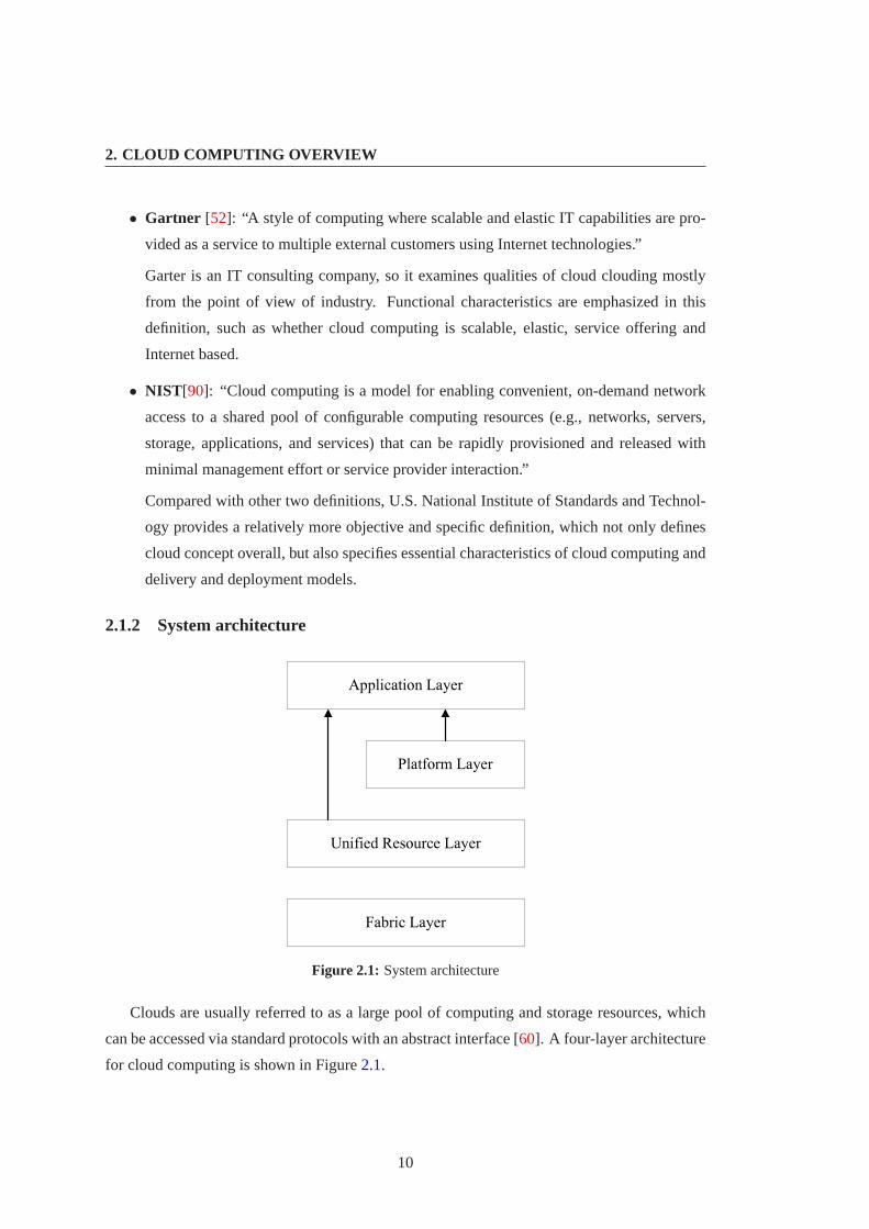
2.1.2 System architecture
Figure 2.1: System architecture
Clouds are usually referred to as a large pool of computing and storage resources, which
can be accessed via standard protocols with an abstract interface [60]. A four-layer architecture
for cloud computing is shown in Figure2.1.
10

2.1 Introduction
The fabric layer contains the raw hardware level resources, such ascompute resources,
storage resources, and network resources. On the unified resource layer, resources have been
virtualized so that they can be exposed to upper layer and end users as integrated resources.
The platform layer adds on a collection of specialized tools, middleware and services on top
of the unified resources to provide a development and deployment platform. The application
layer includes the applications that would run in the clouds.
2.1.3 Deployment models
Clouds are deployed in different fashions, depending on the usage scopes. There are four
primary cloud deployment models.
• Public cloud is the standard cloud computing paradigm, in which a service provider
makes resources, such as applications and storage, available to the general public over
Internet. Service providers charge on a fine-grained utility computing basis. Examples
of public clouds include Amazon Elastic Compute Cloud (EC2), IBM’s Blue Cloud, Sun
Cloud, Google AppEngine and Windows Azure Services Platform.
• Private cloud looks more like a marketing concept than the traditional mainstream sense.
It describes a proprietary computing architecture that provides servicesto a limited num-
ber of people on internal networks. Organizations needing accurate control over their
data will prefer private cloud, so they can get all the scalability, metering, and agility
benefits of a public cloud without ceding control, security, and recurring costs to a ser-
vice provider. Both eBay and HP CloudStart yield private cloud deployments.
• Hybrid cloud uses a combination of public cloud, private cloud and even local infras-
tructures, which is typical for most IT vendors.
Hybrid strategy is proper placement of workloads depending upon costand operational
and compliance factors. Major vendors including HP, IBM, Oracle and VMware create
appropriate plans to leverage a mixed environment, with the aim of delivering services to
the business. Users can deploy an application hosted on a hybrid infrastructure, in which
some nodes are running on real physical hardware and some are running on cloud server
instances.
11
2. CLOUD COMPUTING OVERVIEW
• Community cloud overlaps with Grids to some extent. It mentions that several orga-
nizations in a private community share cloud infrastructure. The organizationsusually
have similar concerns about mission, security requirements, policy, and compliance con-
siderations. Community cloud can be further aggregated by public cloud to build up a
cross-boundary structure.
2.2 Cloud evolution
Although the idea of cloud computing is not new, it has rapidly become a new trendin the
information and communication technology domain and gained significant commercial success
over past years. No one can deny that cloud computing will a play pivotal role in the next
decade. Why cloud computing emerges now, not before? This section looks back on the
development history of cloud computing.
2.2.1 Getting ready for cloud
• Datacenter: Even faster than Moore’s law, the number of servers and datacentershas
increased dramatically in past few years. Datacenter has become the reincarnation of
the mainframe concept. It is easier to build a large-scale commodity-computer datacen-
ter than ever before, just gathering these building blocks together on a parking lot and
plugging them into the Internet .
• Internet : Recently, network performance has improved rapidly. Wired, wireless and 4th
generation mobile communication make Internet available to most of the planet. Cities
and towns are wired with hotspots. The transportation such as air, train, or ship also
equips with satellite based wi-fi or undersea fiber-optic cable. People can connect to the
Internet anywhere and at anytime. The universal, high-speed, broadband Internet lays
the foundation for the widespread applications of cloud computing.
• Terminals: PC is not the only central computing device, various electronic devices in-
cluding MP3, SmartPhone, Tablet, Set-top box, PDA, notebook are new terminals that
have the requirement of personal computing. Besides, repeated data synchronization
among different terminals is time-consuming so that faults occur frequently. In such
cases, a solution that allows individuals to access to personal data anywhere and from
any device is needed.
12

2.2 Cloud evolution
2.2.2 A brief history
Along with the maturity of objective conditions (software, hardware), plenty of existing tech-
nologies, results, and ideas can be realized, updated, merged and further developed.
Amazon played a key role in the development of cloud computing by initially renting their
datacenter to external customers for the use of personal computing. In 2006, they launched
Amazon EC2 and S3 on a utility computing basis. After that, several major vendors released
cloud solutions one after another, including Google, IBM, Sun, HP, Microsoft, Forces.com,
Yahoo and so on. Since 2007, the number of trademarks covering cloud computing brands,
goods and services has increased at an almost exponential rate.
Cloud computing is also a much favored research topic. In 2007, Google, IBM and a
number of universities announced a research project, Academic Cloud Computing Initiative
(ACCI), aiming at addressing the challenges of large-scale distributed computing. Since 2008,
several open source projects have gradually appeared. For example,Eucalyptus is the first
API-compatible platform for deploying private clouds. OpenNebula deploys private and hybrid
clouds and federates different modes of clouds.
In July 2010, SiteonMobile was announced by HP for emerging markets where people are
more likely to access the Internet via mobile phones rather than computers. Withmore and
more people owning smartphones, mobile cloud computing has turned out to be a potent trend.
Several mobile network operators such as Orange, Vodafone and Verizon have started to offer
cloud computing services for companies.
In March 2011, Open Networking Foundation consisting of 23 IT companies was founded
by Deutsche Telecom, Facebook, Google, Microsoft, Verizon, and Yahoo. This nonprofit orga-
nization supports a new cloud initiative called Software-Defined Networking.The initiative is
meant to speed innovation through simple software changes in telecommunications networks,
wireless networks, data centers and other networking areas.
A simple history of cloud development history is presented in Figure2.2.
2.2.3 Comparison with related technologies
Cloud computing is a natural evolution of widespread adoption of virtualization, service-
oriented architecture, autonomic and utility computing. It emerges as a new computing paradigm
to provide reliable, customized and quality services that guarantee dynamic computing envi-
13

2. CLOUD COMPUTING OVERVIEW
Figure 2.2: Cloud development history
ronments for end-users, so it is easily confused with several similar computing paradigms such
as grid computing, utility computing and autonomic computing.
Utility computing
Utility computing was initialized in the 1960s, John McCarthy coined the computer utility
in a speech given to celebrate MIT’s centennial “If computers of the kindI have advocated
become the computers of the future, then computing may someday be organized as a public
utility just as the telephone system is. The computer utility could become the basis ofa new
and important industry.” Generally, utility computing considers the computing and storage
resources as a metered service like water, electricity, gas and telephony utility. The customers
can use the utility services immediately whenever and wherever they need without paying the
initial cost of the devices. This idea was very popular in the late 1960s, butfaded by the mid-
1970s as the devices and technologies of that time were simply not ready. Recently, the utility
idea has resurfaced in new forms such as grid and cloud computing.
Utility computing is highly virtualized so that the amount of storage or computing power
available is considerably larger than that of a single time-sharing computer. The back-end
servers such as computer cluster and supercomputer are used to realizethe virtualization.
Since the late 90’s, utility computing has resurfaced. HP launched the Utility Datacenter to
provide the IP billing-on-tap services. PolyServe Inc. built a clustered filesystem that created
highly available utility computing environments for mission-critical applications and workload
optimized solutions. With utility including database and file service, custumers of vertical
14
2.2 Cloud evolution
industry such as financial services, seismic processing, and content serving can independently
add servers or storage as needed.
Grid computing
Grid computing emerged in the mid 90’s. Ian Foster integrated distributed computing, object-
oriented programming and web services to coin the grid computing infrastructure. “A Grid is
a type of parallel and distributed system that enables the sharing, selection,and aggregation
of geographically distributed autonomous resources dynamically at runtime depending on their
availability, capability, performance, cost, and users’ quality-of-servicerequirements.”[59] The
definition explains that a gird is actually a cluster of networked, loosely coupled computers
which works as a super and virtual mainframe to perform thousands of tasks. It can divide the
huge application job into several subjobs and make each run on large-scale machines.
Generally speaking, grid computing goes through three different generations [103]. The
first generation is marked by early metacomputing environment, such as FAFNERand I-WAY.
The second generation is represented by the development of core grid technologies, grid re-
source management (e.g., GLOBUS, LEGION), resource brokers andschedulers (e.g., CON-
DOR, PBS) and grid portals (e.g., GRID SPHERE). The third generation merges grid comput-
ing and web services technologies (e.g., WSRF, OGSI), and moves to a moreservice oriented
approach that exposes the grid protocols using web service standards.
Autonomic computing
Autonomic computing, proposed by IBM in 2001, performs tasks that IT professionals choose
to delegate to the technology according to policies. [97] Adaptable policy rather than hard
coded procedure determines the types of decisions and actions that autonomic capabilities per-
form. Considering the sharply increasing number of devices, the heterogeneous and distributed
computing systems are more and more difficult to anticipate, design and maintain. The com-
plexity of management is becoming the limiting factor of future development. Autonomic
computing focuses on the self-management ability of the computer system. It overcomes the
rapidly growing complexity of computing systems management and reduces the barriers that
the complexity poses on further growth.
In the area of multi-agent systems, several self-regulating frameworks have been proposed,
with centralized architectures. These architectures reduce management costs, but seldom con-
sider the issues of enabling complex software systems and providing innovative services. IBM
15

2. CLOUD COMPUTING OVERVIEW
proposed the self-managing system that can automatically process, including configuration of
the components (Self-Configuration), automatic monitoring and control of resources to ensure
the optimal (Self-Healing), monitor and optimize the resources (Self-Optimization) and proac-
tive identification and protection from arbitrary attacks (Self-Protection), only with the input
information of policies defined by humans [73]. In other words, the autonomic system uses
high-level rules to check its status and automatically adapt itself to changing conditions.
According to the above introductions of the three computing paradigms, we conclude the
relationship among them. Utility computing concerns whether the packing computing re-
sources can be used as a metered service on the basis of the user’s need. It is indifferent to
the organization of the resources, both in the centralized and distributed systems. Grid com-
puting is conceptually similar to the canonical Foster definition of cloud computing, but it does
not take economic entities into account. Autonomic computing stresses the self management of
computer systems, which is only one feature of cloud computing. All in all, cloud computing
is actually a natural next step from the grid-utility model, having grid technologies, autonomic
characteristics and utility bills.
2.3 Cloud service
As an underlying delivery mechanism, cloud computing ability is provisioned as services, ba-
sically in three levels: software, platform and infrastructure [22].
2.3.1 Software as a Service
Software as a Service (SaaS) is a software delivery model in which applications are accessed by
a simple interface such as a web browser over Internet. The users are not concerned with the un-
derlying cloud infrastructure including network, servers, operating systems, storage, platform,
etc. This model also eliminates the needs to install and run the application on the localcomput-
ers. The term of SaaS is popularized by Salesforce.com, which distributesbusiness software
on a subscription basis, rather than on a traditional on-premise basis. One ofthe best known
is the solution for its Customer Relationship Management (CRM). Now SaaS has now become
a common delivery model for most business applications, including accounting,collaboration
and management. Applications such as social media, office software, and onlinegames enrich
the family of SaaS-based services, for instance, web Mail, Google Docs,Microsoft online,
NetSuit, MMOG Games, Facebook, etc.
16

2.3 Cloud service
2.3.2 Platform as a Service
Platform as a Service (PaaS) offers a high-level integrated environmentto build, test, deploy
and host customer-created or acquired applications. Generally, developers accept some restric-
tions on the type of software that can write in exchange for built-in application scalability.
Customers of PaaS do not manage the underlying infrastructure as SaaS users do, but control
over the deployed applications and their hosting environment configurations.
PaaS offerings mainly aim at facilitating application development and related management
issues. Some are intended to provide a generalized development environment, and some only
provide hosting-level services such as security and on-demand scalability.Typical examples of
PaaS are Google App Engine, Windows Azure, Engine Yard, Force.com,Heroku, MTurk.
2.3.3 Infrastructure as a Service
Infrastructure as a Service (IaaS) provides processing, storage,networks, and other funda-
mental computing resources to users. IaaS users can deploy arbitrary application, software,
operating systems on the infrastructure, which is capable of scaling up and down dynamically.
IaaS user sends programs and related data, while the vendor’s computerdoes the compu-
tation processing and returns the result. The infrastructure is virtualized, flexible, scalable and
manageable to meet user requirements. Examples of IaaS include Amazon EC2, VPC, IBM
Blue Cloud, Eucalyptus, FlexiScale, Joyent, Rackspace Cloud, etc.
Data service concerns user access to remote data in various formats and from multiple
sources. These remote data can be operated just like on a local disk. Amazon S3, SimpleDB,
SQS and Microsoft SQL are data service products. Figure2.3 shows the relationship among
cloud users, clouds services and cloud providers.
Clients equipped with basic devices, Internet and web browsers can directly use software,
platform, storage, and computing resources as pay-as-you-go services. Clouds services are able
to be shared within any one of the service layers, if an Internet protocol connection is estab-
lished. For example, PaaS consumes IaaS offerings, and meanwhile, delivers platform services
to SaaS. At the bottom, datacenter consists of computer hardware and software products such
as cloud-specific operating systems, multi-core processors, networks, disks, etc.
17

2. CLOUD COMPUTING OVERVIEW
Figure 2.3: Cloud service
2.4 Cloud characteristics
As a general resource provisioning model, cloud computing integrates a number of existing
technologies that have been applied in grid computing, utility computing, service oriented ar-
chitectures, internet of things, outsourcing, etc. That is the reason whycloud is mistaken for
“the same old stuff with a new label”. In this section, we distinguish the characteristics of cloud
computing in terms of technical, qualitative and economic aspects.
18

2.4 Cloud characteristics
2.4.1 Technical aspects
Technical characteristics are the foundation that ensures other functional and economical re-
quirements. Not every technology is absolutely new, but is enhanced to realize a specific fea-
ture, directly or as a pre-condition.
• Virtualization is an essential characteristic of cloud computing. Virtualization in clouds
refers to multi-layer hardware platforms, operating systems, storage devices, network
resources, etc.
The first prominent feature of virtualization is the ability to hide the technical complexity
from users, so it can improve independence of cloud services. Secondly, physical re-
source can be efficiently configured and utilized, considering that multiple applications
are run on the same machine. Thirdly, quick recovery and fault toleranceare permitted.
Virtual environment can be easily backed up and migrated with no interruption inservice
[45].
• Multi-tenancy is a highly requisite issue in clouds, which allows sharing of resources
and costs across multiple users.
Multi-tenancy brings resource providers many benefits, for example, centralization of
infrastructure in locations with lower costs and improvement of utilization and effi-
ciency with high peak-load capacity. Tenancy information, which is stored in asepa-
rate database but altered concurrently, should be well maintained for isolated tenants.
Otherwise some problems such as data protection will arise.
• Security is one of the major concerns for adoption of cloud computing. There is no rea-
son to doubt the importance of security in any system dealing with sensitive andprivate
data. In order to obtain the trust of potential clients, providers must supplythe certificate
of security. For example, data should be fully segregated from one to another, and an
efficient replication and recovery mechanism should be prepared if disasters occur.
The complexity of security is increased when data is distributed over a wider area and
shared by unrelated users. However, the complexity reduction is necessary, owing to the
fact that ease-of-use ability can attract more potential clients.
19

2. CLOUD COMPUTING OVERVIEW
• Programming environment is essential to exploit cloud features. It should be capa-
ble of addressing issues such as multiple administrative domains, large variations in re-
source heterogeneity, performance stability, exception handling in highly dynamic envi-
ronments, etc.
System interface adopts web services APIs, which provide a standards-based framework
for accessing and integrating with and among cloud services. Browser, applied as the
interface, has attributes such as being intuitive, easy-to-use, standards-based, service-
independent and multi-platform supported. Through pre-defined APIs, users can access,
configure and program cloud services.
2.4.2 Qualitative aspects
Qualitative characteristics refer to qualities or properties of cloud computing,rather than spe-
cific technological requirements. One qualitative feature can be realized inmultiple ways de-
pending on different providers.
• Elasticity means that the provision of services is elastic and adaptable, which allows
the users to request the service near real-time without engineering for peak loads. The
services are measured in fine-grain, so that the amount of offering canperfectly match
the consumer’s usage.
• Availability refers to a relevant capability that satisfies specific requirements of the out-
sourced services. QoS metrics like response time and throughput must be guaranteed, so
as to meet advanced quality guarantees of cloud users.
• Reliability represents the ability to ensure constant system operation without disruption.
Through using the redundant sites, the possibility of losing data and code dramatically
decreases. Thus cloud computing is suitable for business continuity and disaster recov-
ery. Reliabitiy is a particular QoS requirement, focusing on prevention of loss.
• Agility is a basic requirement for cloud computing. Cloud providers are capable of
on-line reactions to changes in resource demand and environmental conditions. At the
same time, efforts from clients are made to re-provision an application from an in-house
infrastructure to SaaS vendors. Agility requires both sides to provide selfmanagement
capabilities.
20

2.5 Cloud projects
2.4.3 Economic aspects
Economic features make cloud computing distinct compared with other computing paradigms.
In a commercial environment, service offerings are not limited to an exclusive technological
perspective, but extend to a broader understanding of business need.
• Pay-as-you-gois the means of payment of cloud computing, only paying for the ac-
tual consumption of resource. Traditionally, users have to equip with all software and
hardware infrastructure before computing starts, and maintain them during computing
process. Cloud computing reduces cost of infrastructure maintenance and acquisition, so
it can help enterprises, especially small to medium sized, reduce time to market and get
return on the investment.
• Operational expenditure is greatly reduced and converted to operational expenditure
[34]. Cloud users enter the computing world more easily, and they can rent the infras-
tructure for infrequent intensive computing tasks. Minimal technical skills are required
for implementation. Pricing on a utility computing basis is fine-grained with usage-
based options, so cloud providers should mask this pricing granularity with long-term,
fixed price agreements considering the customer’s convenience.
• Energy-efficiencyis due to the ability that a cloud has to reduce the consumption of un-
used resources. Because of central administration, additional costs of energy consump-
tion as well as carbon emission can be better controlled than in uncooperativecases. In
addition, green IT issues are subject to both software stack and hardwarelevel.
2.5 Cloud projects
We conclude the state of the art efforts from commercial and academic sides. Major vendors
have invested in forthright progress in the area of global cloud promotion,while compara-
bly, research organizations based on their funding principles and interest,contribute to cloud
technologies in an indirect way.
2.5.1 Commercial products
In the last few years, a number of middleware and platforms emerge, which involve multiple
level services in heterogeneous, distributed systems. Commercial cloud solutions augment dra-
21

2. CLOUD COMPUTING OVERVIEW
matically and promote organization shift from company-owned assets to per-use service-based
models. The best known cloud projects are Amazon Web Service, Eucalyptus, FlexiScale,
Joyent, Azure, Engine Yard, Heroku, Force.com, RightScale, Netsuite,Google Apps, etc.
Amazon is the pioneer of cloud computing. Since 2002, Amazon has begun to provide
online computing services though Internet. End users, not limited to developers, can access
these web services over HTTP, using Representational State Transfer and SOAP protocols.
All services are billed on usage, but how usage is measured for billing varies from service
to service [128]. Among them, the most popular two are Amazon EC2 and S3, which are
typical representatives of IaaS. The former rents virtual machines forrunning local computing
applications, and the latter offers online storage.
Amazon EC2[1] allows users to create a virtual machine, named instance, through an
Amazon Machine Image. An instance functions as a virtual private server that contains desired
software and hardware. Roughly, instances are classified into 6 categories: standard, micro,
high-memory, high-CPU, cluster-GPU and cluster compute, each of which issubdivided by
the different memory, number of virtual core, storage, platform, I/O performance and API.
Besides, EC2 supports security control of network access, instance monitoring, multi-location
processing etc.
Amazon S3[2] provides a highly durable storage infrastructure used to store and retrieve
data on the Internet. This service is beneficial to developers by making computing more scal-
able. S3 stores data redundantly on multiple devices and supports version control to recover
from both unintended user actions and application failures.
Google App Engine[9], released in 2008, is a platform for developing and hosting web
applications in multiple servers and data centers. In terms of PaaS, GAP is written tobe lan-
guage dependent, and only supports Python and Java, so the runtime environment on GAP is
limited. Compared to IaaS, GAP making it easy to develop scalable applications, but can only
run a limited range of applications designed for that infrastructure.
MapReduce [53] is the best known programming model introduced by Google, which
supports distributed computing on large clusters. It performs map and reduction operations in
parallel. The advantage of MapReduce is that it can efficiently handle large datasets on com-
mon servers and that it can quickly recover from partial failure of servers or storage during
the operation. MapReduce is widely used both in industry and academic research. Google de-
velopes patented framework, while the Hadoop is open source with free license. Besides that,
many projects like Twister, Greenplum, GridGain, Phoenix, Mars, CouchDB, Disco, Skynet,
22

2.5 Cloud projects
Qizmt, Meguro implement the MapReduce programming model in different languages includ-
ing C++, C#, Erlang, Java, Ocaml, Perl, Python, Ruby.
Dryad [7] processing framework was developed by Microsoft as a declarativeprogram-
ming model on top of the computing and storage infrastructure. DryadLINQ targets on writing
large-scale data parallel applications on large data set clusters of computers. DryadLINQ en-
ables developers to use thousands of machines without knowing anything about concurrent
programming. It supports automatic parallelization and serialization by translating LINQ pro-
grams into distributed Dryad computations.
2.5.2 Research projects
Besides company initiatives, a number of academic projects have been developed to address
the challenges including stable testbed, standardization and open source reference implementa-
tion. The most active projects in Europe and North America are XtreemOS, OpenNebula, Fu-
tureGrid, elasticLM, gCube, ManuCloud, RESERVOIR, SLA@SOI, Contrail, ECEE, NEON,
VMware, Tycoon, DIET, BEinGRID, etc.
XtreemOS [16] is an open source distributed operation system for grids. The project was
initialized by INRIA in 2006, and published the first stable release in 2010.
XtreemOS is an uniform computing platform, which integrates heterogeneous infrastruc-
tures, from mobile device to clusters. It provides three services including application execution
management, data management and virtual organization management.
Although XtreemOS was originally designed for grids, it can also be seen as an alternative
for cloud computing, owing to the fact that it is relevant in the context of virtualized distributed
computing infrastructure. Hence, it is able to support cooperation and resource sharing over
cloud federations.
OpenNebula[12] is an open source project aiming at managing datacenter’s virtual infras-
tructure to build IaaS clouds. It was established by Complutense Universityof Madrid in 2005,
and released its first software in 2008.
It supports private cloud creation based on local virtual infrastructurein datacenters, and
has the capabilities for management of user, virtual network, multi-tier services, and physical
infrastructures. It also supports combination of the local resources andremote commercial
cloud to build hybrid clouds, in which local computing capacity is supplemented bysingle or
multiple clouds. In addition, it can be used as interfaces to turn local infrastructure into a public
cloud.
23

2. CLOUD COMPUTING OVERVIEW
FutureGrid [8] is a test-bed for grid and cloud computing. It is a cooperative project
started in 2010 between Grid’5000 and TeraGrid.
FutureGrid builds the federation of multiple clouds with a large geographical distribution,
and allows researchers to study the issues ranging from authentication, authorization, schedul-
ing, virtualization, middleware design, interface design and cybersecurity,to the optimization
of grid-enabled and cloud-enabled computational schemes. The advantageis offering a vivid
cloud platform similar to a real commercial cloud infrastructure. Moreover,it integrates sev-
eral open source technologies to create an easy-to-use environment, such as Xen, Nimbus,
Vine, Hadoop etc.
DIET [6] is a project initiated by INRIA in 2000, which aims at implementing distributed
scheduling strategies on grids and clouds.
DIET developed scalable middleware for a multi-agent system, in which clients submit
computation requests to a scheduler to find a server available on the grid. In order to facilitate
further researches in cloud computing, it supplements cloud-specific elements into scheduler
and adds on-demand resource provision model and economy-based resource model to test pro-
vision heuristics.
SLA@SOI [14] is an European project, targeting on evaluation of service provisioning
based on automated SLA management on SOI.
It developed a SLA management framework, which allows the configuration of multi-layer
service and automation in an arbitrary service-oriented infrastructure. Besides the scientific
values, it implemented a management suit for automated e-contracting and post-sales.
BEinGRID [3] is a research project providing the infrastructure to support pilot implemen-
tations of Grid technologies in actual business scenarios.
In BEinGRID, twenty five business experiments were carried out, each ofwhich focused
on a real business problem and the corresponding solution. To extract best practice from the ex-
perimental implementations, technical and business consultants worked on analysis of generic
components and development of a business plan. Various technologies were evaluated, in-
cluding cost reduction, enhanced processing power, employing new business model, running
Software-as-a-Service application. Although BEinGRID project was concluded, it obtains ex-
periences for cloud computing such as requirement knowledge, businessdrivers, technological
solutions and hinted for migration potential.
24

2.5 Cloud projects
2.5.3 Open areas
Even though some of the essential characteristics of cloud computing have been realized by
commercial and academic efforts, not all capabilities are fulfilled to the necessary extent. Sev-
eral challenges are identified as follows
Middleware
Cloud-enablement functions for an application are brought by web servers, web portals,
identity management servers, load balancers and application servers. In order to coordinate and
use them harmoniously, middleware continues to play a key role in cloud computing. Generally
speaking, cloud middleware is the software used to integrate services, applications and content
available on the same or different layers, by which services and other software components can
be reused through Internet.
Platform virtualization
Virtualization is one of the crucial technologies that can merge different infrastructures,
and the management of virtual machines needs to be further developed. Since there are a lot of
mature middleware used in grid computing, how to combine them with cloud middleware isa
matter of our concern. Even more, natural evolution from grid to cloud is important, because
effort and time can be saved by technology reuse.
Programming model
As the migration to cloud is inevitable, programming and accessing cloud platforms should
perform in a seamless and efficient way. In the future, computational platforms will have a huge
number of processing nodes, so traditional parallelization models such as batch processing and
message passing models are not scalable enough to deal with large scale distributed computing.
Resource management
Form the provider’s point of view, large scale of virtual machines needsto be allocated to
thousands of distributed users, dynamically, fairly, and most important, profitably. From the
consumer’s point of view, users are economy-driven entities when theymake the decision to
use cloud service [44]. For adequate resource, one user will compare the price among different
providers. For scarce resource, users themselves become competitors who will impact the
future price directly, or indirectly. Therefore, the future resource provisioning will become a
multi-objective and multi-criteria problem.
For practical reasons, resource provisioning needs reliable and efficient support of nego-
tiation, monitoring, metering, and feedback. Service Level Agreement (SLA)is a common
25

2. CLOUD COMPUTING OVERVIEW
tool to define contracts and to measure fulfillments in business scenarios. Itdescribes a set of
non-functional requirements of the service, and includes penalties when the requirements are
not met. Therefore, formal means for contract description have to be standardized.
2.6 Summary
In this chapter, the concept of cloud computing is first introduced. Although there is vast dis-
agreement over what cloud computing is, we try to refine some representatives and give an
unbiased and general definition. That definition is not just an overall concept, but describes
system architecture, deployment model and essential features. Cloud computing is still an
evolving paradigm, and it integrates many existing technologies. A brief retrospect of evo-
lution history helps us clarify the conditions, opportunities and challenges existingin cloud
development. These definitions, attributes, and characteristics will evolve and change over
time.
Functionally speaking, cloud computing is a service provision model, where software, plat-
form, infrastructure, data, hardware can be directly delivered as a service to end customers. The
service characteristics are presented from technical, qualitative and economic aspects.
Current efforts are the foundation for further development. After analyzing existing com-
mercial products and research projects, several challenges in terms ofmiddleware, program-
ming model, resource management and business model are highlighted. Thesegaps in cloud
computing inspire our interest in our future research. In the following chapters, the problem of
resource management is discussed from micro- and macro- aspects. In particular, issues such
as resource allocation and job scheduling are studied.
26

3
Scheduling problems for cloud
computing
3.1 Introduction
This chapter outlines the scheduling problems arising from cloud computing. Concerned theo-
ries including former expressions of problems, algorithms, complexity and schematic methods
are briefly introduced. Then scheduling hierarchy in cloud datacenter is presented, by splitting
scheduling problem into user-level and system-level. The former focuses on resource provi-
sion issues between providers and customers, which are solved by economic models. The latter
refers to meta-task execution, a sub-optimal solution of which is given by heuristics to speed
up the process of finding a good enough answer. Moreover, real-time scheduling attracts our
attention. Different from economic and heuristic strategies, priority scheduling algorithms and
their implementation are discussed at the end of this chapter.
3.2 Scheduling problems
3.2.1 Problems, algorithms and complexity
Scheduling problem [33] is the problem of matching elements from different sets, which is
formally expressed as a triple (E, S, O), where
• E is the set of examples, each of which is an instance of problem.
• S is the set of feasible solutions for the example.
27

3. SCHEDULING PROBLEMS FOR CLOUD COMPUTING
• O is the object of the problem.
Scheduling problem can be further classified into two categories dependingon objectO:
optimization problem and decision problem. An optimization problem requires findingthe
best solution among all the feasible solutions in setS. Different from optimization, the aim of
decision problem is relatively easy. For a specified feasible solutions ∈ S, problem needs a
positive or negative answer to whether the objectO is achieved. Clearly, optimization problem
is harder than decision problem, because the specified solution only compares with one thresh-
old solution in decision problem, instead of all feasible solutions in optimization problem.
An algorithm is a collection of simple instructions for finding a solution to a problem.
It contains three parts: input, method, output. Input is a set of parametersto be dealt with.
Method includes describable, controllable, repeatable procedures to realize the aim using input
parameters. Output is a result of the problem. Especially for scheduling, thealgorithm is
a method by which tasks are given access, matched, or allocated to processors. Generally
speaking, no absolutely perfect scheduling algorithm exists, because scheduling objectives may
conflict with one another. A good scheduler implements a suitable compromise, or applies
combination of scheduling algorithms according to different applications.
A problem can be solved in seconds, hours or even years depending onthe algorithm ap-
plied. The efficiency of an algorithm is evaluated by the amount of time necessary to execute
it. The running time of an algorithm is stated as a time complexity function relating the input
length to the number of steps.
There are several kinds of time complexity algorithms that will appear in the following
chapters.
• For a constant time algorithmO(1), the maximum amount of running time is bounded
by a value that does not rely upon the size of the input.
• For a linear time algorithmO(n), the maximum amount of running time increases lin-
early with the size of the input.
• For a polynomial time algorithmO(nc) with a constantc, the maximum amount of
running time is bounded by a polynomial expression in the size of the input.
• For a exponential time algorithmO(2nc) with a constantc, the maximum amount of
running time is bounded by an exponential expression in the size of the input.
28

3.2 Scheduling problems
If a problem has a polynomial time algorithm, the problem is tractable, feasible, efficient or
fast enough to be executed on a computational machine. In computational complexity theory, a
complexity class is a set of problems that has the same complexity based on a certain resource
[110].
• Class P is the set of decision problems that are solvable in polynomial time on a deter-
ministic Turing machine, which means that a problem of Class P can be decided quickly
by a polynomial time algorithm.
• Class NP is the set of decision problems that are solvable in polynomial time on a non-
deterministic Turing machine, but a candidate solution of the problem of Class NPcan be
verified by a polynomial time algorithm, which means that the problem can be verified
quickly.
• Class NP-complete is the set of decision problems, to which all other NP problems can
be polynomial transformable, and a NP-complete problem must be in class NP.Generally
speaking, NP-complete problems are more difficult than NP problems.
• Class NP-hard is the set of optimization problems, to which all NP problems can be
polynomial transformable, but a NP-hard problem is not necessarily in class NP.
Although most of NP-complete problems are computationally difficult, some of them are
solved with acceptable efficiency. There are some algorithms, the running time of which is
not only bounded by the size of input of an example, but also by the maximum number of the
examples. These algorithms have pseudopolynomial time complexity. For one problem, if its
maximum number is not large, it can be solved quickly. Thus, one NP-completeproblem with
known pseudo-polynomial time algorithms is called weakly NP-complete, otherwiseis called
strongly NP-complete, if it can not be solved by a pseudopolynomial time algorithm unless
P=NP [110].
3.2.2 Schematic methods for scheduling problem
Scheduling problems belong to a broad class of combinational optimization problems aiming
at finding an optimal matching from a finite set of objects, so the set of feasible solutions is
usually discrete rather than continuous. An easy problem refers to one with asmall number
of the examples, so it can be simply worked out by polynomial algorithms or enumerations.
29

3. SCHEDULING PROBLEMS FOR CLOUD COMPUTING
On the contrary a problem is in Class NP-complete if its purpose is making a decision, and
is in Class NP-hard if its purpose is optimization. Because an optimization problem is not
easier than a decision problem, we only list schematic methods for NP-hard problems. As
shown in Figure3.1, enumeration, heuristic and approximation are three possible solutions,
their corresponding algorithms complement each other to give a relatively good answer to a
NP-hard problem.
Figure 3.1: Schematic view
Enumeration method
For an optimization problem, its optimal solution can be selected if all the possible solutions are
enumerated and compared one by one. Exact enumerative algorithms have the exponential time
complexity in the worst case. However, for some NP-hard problems in weaksense, when the
number in one instance is relatively small, it can be solved by a pseudopolynomial algorithm,
the time complexity of which is bounded by a polynomial expression of the input size and the
maximum number of the problem.
Moreover, there is another kind of enumeration, called implicit enumeration, which eval-
uates all possible solutions without explicitly listing all of them. Dynamic programming is a
practicable implicit enumeration method to solve combinational optimization problems. It di-
vides a problem into a number of stages, and at each stage a decision is required, impacting on
the decisions to be made at later stages. The number of stored decisions is exponential to the
number of subproblems, so the worst complexity function of dynamic programmingalgorithms
is exponential.
30

3.2 Scheduling problems
Heuristic method
Exhaustive enumeration is not feasible for scheduling problems, because only a few special
cases of NP-hard problems have exactly-solvable algorithms in polynomial time. For the sake
of practice, we tend to find suboptimal solutions that are good enough to balance accuracy and
time.
Heuristic is a suboptimal algorithm to find reasonably good solutions reasonablyfast. It
iteratively improves a candidate solution with regard to a given measure of quality, but does
not guarantee the best solution. To be more precise, approximation raterH(e) is introduced to
evaluate the accuracy of heuristic algorithms [33].
rH(e) =H(e)
OPT (e)(3.1)
whereH(e) is the value of the solution constructed by heuristicH for instancee, and
OPT (e) is the value of the optimal solution fore. If there is an integerK, all the instances
satisfyOPT (e) ≥ K, this asymptotic ratiorH can be used to measure the quality of approx-
imation algorithm. The closerrH approaches one, the better the performance is achieved by
heuristics.
With greedy rules, several common algorithms are shown as follows.
• Next Fit heuristic: The simplest algorithm for bin-packing problem. Each object is as-
signed to the current bin if it fits, otherwise, it is assigned to a new bin. Approximation
rate isrNF ≤ 2.
• First Fit heuristic: Each object is assigned to the lowest initialized indexed binif it fits.
A new bin is created only if the new object can not fit any initialized bin. Approximation
rate isrFF ≤ 7/4.
• Best Fit heuristic: Each object is assigned to the smallest residual bin if it fits. A new
bin is created only if the new object can not fit any initialized bin. Approximation rate is
rBF ≤ 7/4.
• Next/First/Best Fit Descending heuristic: Objects are first sorted in descending order,
and then are assigned by corresponding heuristics. Approximation rate isrxFD ≤ 3/2.
31
3. SCHEDULING PROBLEMS FOR CLOUD COMPUTING
Relaxation method
Another feasible method to solve NP-hard problems is relaxing some constraints imposed on
the original problem. In the new relaxed problem, the solution might be easy to obtain and
have a good approximation to that in the original problem. The common relaxation includes:
• Suppose the elements in one instance are all natural numbers, rather than real numbers.
• Suppose the value of one special element remains unchanged, rather thanvaried.
• Suppose the value of two interrelated elements equal, rather than one being bounded by
the other.
• Suppose the value of one element is unit, rather than arbitrary.
• Suppose the type of one element is certain, rather than arbitrary.
More relaxation can be applied without the limit of above presentation.
3.3 Scheduling hierarchy in cloud datacenter
In last section, we introduced related theory about scheduling problems andtheir schematic
methods. From this section, we specify scheduling problems in cloud environments. As a key
characteristic of resource management, service scheduling makes cloud computing different
from other computing paradigms. Centralized scheduler in cluster system aims at enhancing
the overall system performance, while distributed scheduler in grid systemaims at enhancing
the performance of specific end-users. Compared with them, scheduling in cloud computing
is much more complicated. On one hand, centralized scheduler is necessary, because every
cloud provider, which promises to provide services to users without reference to the hosted
infrastructure, has an individual datacenter. On the other hand, distributed scheduler is also
indispensable, because commercial property determines that cloud computing should deal with
the QoS requirements of customers distributed worldwide.
An important issue of this chapter is to decompose scheduling problems related tocloud
computing. Since cloud service is actually a virtual product on a supply chain, the service
scheduling can be classified into two basic catagories: user-level and system-level. The hierar-
chy is shown in Figure3.2. The user-level scheduling deals with the problem raised by service
provision between providers and customers. It mainly refers to economic concerns such as
32

3.3 Scheduling hierarchy in cloud datacenter
Figure 3.2: Scheduling hierarchy
equilibrium of supply and demand, competition among consumers and cost minimization un-
der elastic consumer preference. The system-level scheduling handles resource management
within a datacenter. From the point of view of customers, a datacenter is an integration system,
which provides uniform services. Actually, the datacenter consists of many physical machines,
homogeneous or heterogeneous. After receiving numerous tasks from different users, assign-
ing tasks to physical machines significantly impacts the performance of datacenter. Besides
improving the system utilization, some specific requirements should be considered, such as the
real-time satisfaction, resource sharing, fault tolerance, etc.
33

3. SCHEDULING PROBLEMS FOR CLOUD COMPUTING
3.4 Economic models for resource-provision scheduling
In the past three years, explosion of supply-side cloud service provision has accelerated, cloud
solutions become mainstream productions of IT industry. At the same time, these cloud ser-
vices gradually mature to become more appropriate and attractive to all types of enterprises.
The growth of both sides of supply and demand makes the scheduling problems more com-
plex, sophisticated, and even vital in cloud environment. A bad scheduling scheme not only
undermines CPU utilization, turnaround time and cumulative throughput, but may also result
in terrible consequences, for example providers lose money and even goout of business.
Economic models are more suitable for cloud-based scheduling than traditional multipro-
cessor models, especially for regulating the supply and demand of cloud resources. In eco-
nomics, market-based and auction-based schedulers handle two main interests. Market-based
schedulers are applied when a large number of naive users can not directly control service
price in commodity trade. Mainstream cloud providers apply market-based pricing schemes
in reality. The concrete schemes vary from provider to provider. As the most successful IaaS
provider, Amazon EC2 supports commodity and posted pricing models for the convenience of
users. Another alternative is auction-based scheduler, which is adaptedto situations where a
small number of strategic users seeking to attain a specific service compete witheach other. In
auctions, users are able to commit the auction price. Amazon spot instance is an example of
auction-based model. Instance price adjusts from time to time, depending on the supply and
demand. As a result, users should estimate the future price and make its proposal in an auction
before placing a spot instance request.
3.4.1 Market-based strategies
In cloud service provision, both service providers and users express their requirements through
SLAs contracts. Providers need mechanisms that support price specification and increase sys-
tem utilization, while consumers need schemes that guarantee their objectives are reached. A
market-based scheduler aims at regulating the supply and demand for resources. To be spe-
cific, the market strategies emphasize the schemes for establishing a serviceprice depending
on their customers’ requirements. In previous literature, a broker behaving on the behalf of
one end-user interacts with service providers to determine a proper pricethat keeps supply and
demand in equilibrium [40].
34

3.4 Economic models for resource-provision scheduling
Strategy types
Commodity model
As a common model in our daily life, service providers specify their service price and
charge users according to the amount of resource they consume. Any user is free to choose
a proper provider, but has no right to change the service price directly. The amount of their
purchase can cause the price to derive from supply and demand.
The process of scheduling is executed by brokers. On the behalf of users, each broker
identifies several providers to inquire the prices, and then selects one provider which can meet
its objective. The consumption of service is recorded and payment is made as agreed.
Posted price model
The posted price strategy makes some special offers to increase the market share or to
motivate customers to use the service during the off-peak period. The posted price, as a kind
of advertisement, has time or usage limitations that are not suitable for all users.Therefore, the
scheduling process should be modified in this strategy.
Service providers give the regular price, the cheap offers and the associated conditions of
usage. Brokers observe the posted price, and compare whether it canmeet the requirement of
users. If not, brokers apply commodity strategy as usual. Otherwise, brokers only inquire the
provider for availability of posted services, supplementing extra regular service when associ-
ated conditions are not satisfied.
Bargaining model
In bargaining strategy, price is not given by provider unilaterally, but by both sides of the
transaction through bargaining. A prerequisite for bargaining is that the objective functions for
providers and brokers must have an intersection, so that they can negotiate with each other as
long as their objectives are both met.
In this scenario, a broker does not compare all the prices for the same service, but connects
with one of the providers directly. The price offered by the provider mightbe higher than
customer expectation, so the broker starts with a very low price, which has theupside potential.
The bargaining ends when a mutually agreeable price is reached or when one side is not willing
to negotiate any further. In the latter case, broker will connect with other providers and then
start bargaining again.
Bargaining strategy has an obvious shortcoming, that is, the overhead oncommunication
is very high. The time delay might lead to lower utilization of resources for the provider or
35

3. SCHEDULING PROBLEMS FOR CLOUD COMPUTING
shorten deadline of service for the customers. In reality, the number of negotiations can not be
infinite, and the bargaining time is always limited.
Principles for strategy design
Several market principles should be considered in the process of determining the service price
[115].
Equilibrium price refers to a price under which the amount of services bought by buyers
is equal to the amount of services produced by sellers. This price tends tobe stable unless
demand or supply change.
Pareto efficiencydescribes a situation where no agent can get a better allocation than the
initial one without reducing other individual allocations. In other words, resource can not be
reallocated in a way that makes everyone better off.
Individual rationality can make price fluctuate around the equilibrium price, which is
determined by the process of supply and demand. A higher price providesincentive to produce
more resource, so the amount of scarce resource can gradually reach saturation then surplus,
and vice-versa. Individual rationality can adjust prices to reach equilibrium instantaneously.
Stability examines whether a scheduling mechanism can be manipulated. Individual agent
may not reveal private information truthfully. A stable mechanism allows agentsto obtain the
best allocation if they submit their truthful information.
Communication efficiencyevaluates the communication overhead to capture a desirable
global solution. Message passing adds communication overhead on transaction, so additional
time is spent on allocation, rather than on computation. A good scheduling mechanism finds
out a near-optimum solution efficiently.
3.4.2 Auction strategies
Unlike in market-based models, an auction-based scheduler is a rule maker, rather than a price
maker. The rules include how the users bid for services, how the sale price is determined,
who the winning bidder is, how the resource is allocated, whether there are limitson time or
proposal price, etc.
In auction-based schedulers, price is decided according to the given rules, which benefits
consumers by expressing their real requirement strategically, rather than waiting for price ad-
36

3.4 Economic models for resource-provision scheduling
justment in a passive manner. Auction-based schedulers are distinguished from each other by
several characteristics.
Strategy types
Number of participants
According to different numbers of bidders, auctions are classified into demand auction,
supply auction and double auction. English auction is an example of demand auction,in which
n buyers bid for one service. This type of auction is the most common form of auctionin use
today. Dutch auction focuses on demand of suppliers, wherem sellers offer the same service
for one buyer.
Double auction is needed under the condition that the number of buyers and sellers is more
than one. In double auction, sellers and buyers both offer bids. The amount of trade is decided
by the quantity at which the marginal buy bid is higher than the marginal sell bid.With the
growing number of participants, double auction converges to the market equilibrium.
Information transparency
Participants in an auction may or may not know the actions of other participants. Both
English and Dutch auctions are open auctions, that is, the participants repeatedly bid for the
service with the complete information about previous bids of other bidders. Apart from these,
there is another type of auction, in which participants post sealed bids and thebidder with
highest bid wins. In close auction, bidders can only submit one bid each andno one knows the
other bids. Consequently, blind bidders cannot adjust their bids accordingly.
Close auction is commonly used for modeling resource provision in multi-agent system,
considering the simplicity and effectiveness of the sealed bids.
Combinatorial auction
A combinatorial auction is a type of smart market in which participants can place bids on
combinations of items, rather than just individual items. Combinatorial auction is appropriate
for computational resource auction, where a common procedure accepts bidsfor a package of
items such as CPU cycles, memory, storage, and bandwidth.
Combinatorial auctions are processed by bidders repeatedly modifying their proposals until
no one increases its bid any more. In each round, auctioneer publishes a tentative outcome to
help bidders decide whether increase their bids or not. The tentative outcome is the one that
can bring auctioneer the best revenue given the bids. However, finding an allocation of items
to maximize the auctioneer’s revenue is NP-complete. A challenge of combinatorial auctions
37

3. SCHEDULING PROBLEMS FOR CLOUD COMPUTING
comes from how to efficiently determine the allocation once the bids have been submitted to
the auctioneer.
Proportion shared auction
In proportion shared auctions, no winner exists, but all bidders share thewhole resource
with a percentage based on their bids. This type of auction guarantees a maximized utility
and ensures fairness among users in resource allocation, which suits limited resource such as
time slot, power and spectrum bandwidth [76]. Shares represent relative resource rights that
depend on the total number of shares contending for a resource. Clientallocations degrade
gracefully in overload situations, and clients proportionally benefit from extraresources when
some allocations are underutilized.
Principles for strategy design
Game theoretical equilibrium
The auction models applied in cloud service and other computational resource provisioning
are listed above, but not limited to these primary types. Generally, auction-based scheduler
emphasizes the equilibrium among users rather than supply-demand balance between provider
and user. The effectiveness of auction can be analyzed with the help of game theory.
Game theory studies multi-person decision making problems. Any player involved in a
game makes the best decision, taking into account decisions of the others. Agame theoretical
equilibrium is a solution, in which no player gains by only changing his own strategy unilat-
erally. However, this equilibrium does not necessarily mean the best cumulative payoff for all
players.
Incentive compatibility
In any auction, participants might hide their true preferences. Incentive compatible auction
is one in which participants have incentive to reveal their real private information. One bidder
can maximize his payoff only if the information is submitted truthfully.
One method to realize incentive compatibility is designing a reasonable price payed by
auction winner. A good example of incentive compatible auction is Vickery auction. In this
sealed price auction, the highest bidder wins, but pays the second highest bid rather than his
own. Under this charging rule, biding lower or higher than his true valuation will never increase
the best possible outcome.
38

3.4 Economic models for resource-provision scheduling
3.4.3 Economic schedulers
Economic schedulers have been applied to solve resource management in various computing
paradigms, such as cluster, distributed databases, grids, parallel systems, Peer-to-Peer, and
cloud computing [44]. Existing middleware applying economic schedulers, not limited to cloud
platforms, are introduced. By doing this, we can examine the applicability and suitability
of these economic schedulers for supporting cloud resource allocation in practice. This in
turn helps us identify possible strengths of these middleware that may be leveraged for cloud
environment.
Cluster-on-demand[4] is a service-oriented architecture for networked utility computing.
It creates independent virtual clusters for different groups. These virtual clusters are assigned
and managed by a cluster broker, supporting tendering and contract-net economic model. The
user submits its requirements to all cluster brokers. Every broker proposes a specific contract
with the estimated execution time and cost. If the number of brokers proposing contacts is
more than one, users then select only one of them as the resource provider. Earning is afforded
by users to cluster broker as costs for adhering to the conditions of the contract.
Mosix [11] is a distributed operating system for high performance cluster computing that
employs an opportunity cost approach to minimize the overall execution cost ofthe cluster.
It applies commodity model to compute a single marginal cost based on the processor and
memory usages of the process. The cluster node with the minimal value of marginal cost is
then assigned the process.
Stanford Peers[15]is a peer-to-peer data trading framework, in which both auction and
bartering models are applied. A local site wishing to replicate its collection holds anauction to
solicit bids from remote sites by first announcing its request for storage space. Each interested
remote site then returns a bid, and the site with the lowest bid for maximum benefit isselected
by the local site. Besides that, a bartering system supports a cooperativetrading environment
for producer and consumer participants, so that sites exchange free storage spaces to benefit
both themselves and others. Each site minimizes the cost of trading, which is the amount of
disk storage space that it has to provide to the remote site for the requested data exchange.
D’Agents [5] is a mobile-agent system for distributed computing. It implements proportion
shared auction where agents compete for shared resources. If there ismore than one bidder,
resources are allocated proportionally. Costs are defined as rates, such as credits per minute to
reflect the maximum amount that a user wants to pay for the resource.
39

3. SCHEDULING PROBLEMS FOR CLOUD COMPUTING
Nimrod-G [19] is a tool for automated modeling and execution of parameter sweep appli-
cations on Grids. Through broker, the grid users obtain service prices from different resources.
Deadline and budget are main constraints specified by the user for runninghis application.
The allocation mechanisms are based on market-based models. Prices of resources thus vary
between different executing applications depending on their QoS constraints.A competitive
trading environment exists, because users have to compete with one anotherin order to maxi-
mize their own personal benefits.
Faucets[71] is a resource scheduler of computational grid, and its objective is supporting
efficient resource allocation for parallel jobs executed on a changing number of allocated pro-
cessors during runtime on demand. Tendering model is used in Faucets. A QoS contract is
agreed before job execution, including payoff at soft deadline, a decreased payoff at hard dead-
line and penalty after hard deadline. Faucets aims to maximize the profit of resource provider
and resource utilization.
MarketNet [51] is a market-based protection technology for distributed information sys-
tems. Posted price model is incorporated. Currency accounts for information usage. MarketNet
system advertises resource request by offering prices on a bulletin board. Through observing
currency flow, potential intrusion attacks into the information systems are controlled, and the
damages are kept to the minimum.
Cloudbus [42] is a toolkit providing market-based resource management strategies to me-
diate access to distributed physical and virtual resources. A 3rd party cloud broker is built on
an architecture that provides a general framework for any other cloudplatforms. A number of
economic models with commodity, tendering and auction strategies are available for customer-
driven service management and computational risk management. The brokersupports various
application models such as parameter sweep, workflow, parallel and bag of tasks. It has plug-in
support for integration with other middleware technologies such as Globus, Aneka, Unicore,
etc.
OpenPEX [122] is a resource provisioning system with an advanced reservation approach
for allocating virtual resources. A user can reserve any number of instances of virtual machine
that have to be started at a specific time and have to last for a specific duration. A bilateral
negotiation protocol is incorporated in OpenPEX, allowing users and providers to exchange
their offers and counter-offers, so more sophisticated bartering or double auction models are
helpful to improve revenue of cloud users.
40

3.5 Heuristic models for task-execution scheduling
EERM [56] is a resource broker that enables bidirectional communication between busi-
ness and resource layers to promote good decision-making in resource management. EERM
contains sub-components for performing pricing, accounting, billing, job scheduling, moni-
toring and dispatching. It uses kinds of market-based mechanisms for allocating network re-
sources. To increase the revenue, overbooking strategy is implemented tomitigate the effects
of cancellations and no-shows.
A summary of economic schedulers is concluded in Table3.1.
Table 3.1: Economic schedulers
Scheduler Economic model Computing paradigm
Cluster-on-demand tendering cluster
Mosix commodity cluster
Stanford Peers auction/bartering peer to peer
D’Agents proportion shared auction mobile-agent
Faucets tendering grid
Nimrod-G commodity/auctions grid
Marketnet posted price distributed information
Cloudbus commodity/tendering/auctions cloud
OpenPEX bartering/double auction cloud
EERM commodity/posted price/bartering/tenderingcloud
3.5 Heuristic models for task-execution scheduling
In cloud computing, a typical datacenter consists of commodity machines connectedby high-
speed links. This environment is well suited for the computation of large, diverse group of
tasks. Tasks belonging to different users are no longer distinguished one from another. Schedul-
ing problem in such a context turns out to be matching multi tasks to multi machines.As
mentioned in the former section, the optimal matching is an optimization problem, generally
with NP-complete complexity. Heuristic is often applied as a suboptimal algorithm to obtain
relatively good solutions.
This section intensively researches two types of strategies, static and dynamic heuristics.
Static heuristic is suitable for the situation where the complete set of tasks is known prior to
41

3. SCHEDULING PROBLEMS FOR CLOUD COMPUTING
execution, while dynamic heuristic performs the scheduling when a task arrives. Before further
explanation, several preliminary terms should be defined.
• ti: taski
• mj : machinej
• ci: the time when taskti comes
• aj : the time when machinemj is available
• eij : the execution time forti is executed onmj
• cij : the time when the execution ofti is finished onmj , cij = aj + eij
• makespan: the maximum value ofcij , which means the whole execution time. The aim
of heuristics is to minimize makespan, that is to say, scheduling should finish execution
of metatask as soon as possible.
3.5.1 Static strategies
Static strategies are performed under two assumptions. The first is that tasksarrive simulta-
neouslyci = 0. The second is that machine available timeaj is updated after each task is
scheduled.
OLB (Opportunistic Load Balancing) schedules every task, in arbitrary order, to next avail-
able machine. Its implementation is quite easy, because it does not need extra calculation. The
goal of OLB is simply keeping all machines as busy as possible.
MET (Minimum Execution Time) schedules every task, in arbitrary order, to the machine
which has the minimum execution time for this task. MET is also very simple, giving the best
machine to each task, but it ignores the availability of machines. MET jeopardizes the load
balance across machines.
MCT (Minimum Completion Time) schedules every task, in arbitrary order, to the ma-
chine which has the minimum completion time for this task. However, in this heuristic, not all
tasks can be given the minimum execution time.
Min-min begins with the setT of all unscheduled tasks. Then, the matrix for minimum
completion time for each task in setT is calculated. Task with overall minimum completion
42

3.5 Heuristic models for task-execution scheduling
time is scheduled to its corresponding machine. Next, the scheduled task is removed fromT .
The process repeats until all tasks are scheduled.
Min-max is similar to Min-min heuristic. Min-max also begins with the setT of all un-
scheduled tasks, and then calculates the matrix for minimum completion time for each task in
setT . Different from min-min, task with overall maximum completion time is selected and
scheduled to its corresponding machine. Next, the scheduled task is removed from T . The
process repeats until all tasks are scheduled.
GA (Genetic Algorithm) is a heuristic to search for a near-optimal solution in large solu-
tion spaces [36]. The first step is randomly initializing a population of chromosomes (possible
scheduling) for a given task. Each chromosome has a fitness value (makespan) that results from
the scheduling of tasks to machines within that chromosome. After the generation of the initial
population, all chromosomes in the population are evaluated based on their fitness value, with a
smaller makespan being a better mapping. Selection scheme probabilistically duplicates some
chromosomes and deletes others, where better mappings have a higher probability of being
duplicated in the next generation. The population size is constant in all generations. Next, the
crossover operation selects a random pair of chromosomes and choosesa random point in the
first chromosome. Crossover exchanges machine assignments between corresponding tasks.
Mutation operation is performed after crossover. Mutation randomly selects a chromosome,
then randomly selects a task within the chromosome, and randomly reassigns it to anew ma-
chine. After evaluating the new population, another iteration of GA starts, including selection,
crossover, mutation and evaluation. Only when stopping criteria are met, the iteration will stop.
SA (Simulated Annealing) uses a procedure that probabilistically allows poorer solutions
to be accepted to obtain a better search of the solution space. This probability isbased on a
system temperature that decreases for each iteration, which implies that a poorer solution is
difficulty to be accepted. The initial system temperature is the makespan of the initial schedul-
ing, which is mutated in the same manner as the GA. The new makespan is evaluatedat the
end of each iteration. A worse makespan might be accepted based on a probability, so the SA
finds poorer solutions than Min-min and GA.
Tabu search keeps track of the regions of the solution space which have already been
searched so as not to repeat a search near these areas. A scheduling solution uses the same
representation as a chromosome in the GA approach. To manipulate the current solution and
to move through the solution space, a short hop is performed. The intuitive purpose of a
short hop is to find the nearest local minimum solution within the solution space. Whenthe
43

3. SCHEDULING PROBLEMS FOR CLOUD COMPUTING
short hop procedure ends, the final scheduling from the local solution space search is added
to the tabu list. Next, a new random scheduling is generated, to perform a longhop to enter
a new unsearched region of the solution space. After each successfullong hop, the short hop
procedure is repeated. After the stopping criterion is satisfied, the best scheduling from the
tabu list is the final answer.
A∗ is a tree-based search heuristic beginning at a root node that is a null solution. As the
tree grows, nodes represent partial scheduling (a subset of tasks is assigned to machines), and
leaves represent final scheduling (all tasks are assigned to machines).The partial solution of a
child node has one more task scheduled than the parent node. Each parent node can be replaced
by its children. To keep execution time of the heuristic tractable, there is a pruningprocess to
limit the maximum number of active nodes in the tree at any one time. If the tree is notpruned,
this method is equivalent to an exhaustive search. This process continues until a leaf (complete
scheduling) is reached.
The listed heuristics above are fit for different scheduling scenarios. The variation of sce-
narios is caused by the task heterogeneity, machine heterogeneity and machine inconsistence.
The machines are consistent if machinemi executes any task faster than machinemj , it exe-
cutes all tasks faster thanmj . These heuristics are evaluated by simulation in article [36]. For
consistent machines, GA performs the best, while MET performs the worst. For inconsistent
machines, GA andA∗ give the best solution, and OLB gives the worst. Generally, GA,A∗ and
min-min can be used as a promising heuristic with short average makespan.
3.5.2 Dynamic strategies
Dynamic heuristics are necessary when task set or machine set is not fixed. For example, not all
tasks arrive simultaneously, or some machines go offline at intervals. The dynamic heuristics
can be used in two fashions, on-line mode and batch mode. In the former mode,a task is
scheduled to a machine as soon as it arrives. In the latter mode, tasks are firstly collected into
a set that is examined for scheduling at prescheduled times.
On-line mode
In on-line heuristics, each task is scheduled only once, the scheduling result can not be changed.
On-line heuristic is suitable for the cases in which arrival rate is low [109].
44

3.5 Heuristic models for task-execution scheduling
OLB dynamic heuristic assigns a task to the machine that becomes ready next regardless
of the execution time of the task on that machine.
MET dynamic heuristic assigns each task to the machine that performs that task’s compu-
tation in the least amount of execution time regardless of machine available time.
MCT dynamic heuristic assigns each task to the machine, which results in task’s earliest
completion time. MCT heuristic is used as a benchmark for the on-line mode [109].
SA (Switching Algorithm) uses the MCT and MET heuristics in a cyclic fashion depending
on the load distribution across the machines. MET can choose the best machine for tasks but
might assign too many tasks to same machines, while MCT can balance the load, butmight
not assign tasks machines that have their minimum executing time. If the tasks are arriving
in a random mix, it is possible to use the MET at the expense of load balance upto a given
threshold and then use the MCT to smooth the load across the machines.
KPB (K-Percent Best) heuristic considers only a subset of machines while scheduling a
task. The subset is formed by picking thek best machines based on the execution times for
the task. A good value ofk schedules a task to a machine only within a subset formed from
computationally superior machines. The purpose is to avoid putting the current task onto a
machine which might be more suitable for some yet-to-arrive tasks, so it leadsto a shorter
makespan as compared to the MCT.
For all the on-line mode heuristics, KPB outperforms others in most scenarios[109]. The
results of MCT are good, only slightly worse than KPB, owing to the lack of prediction for task
heterogeneity.
Batch mode
In batch mode, tasks are scheduled only at some predefined moments. This enables batch
heuristics to know about the actual execution times of a larger number of tasks.
Min-min firstly updates the set of arrival tasks and the set of available machines,calcu-
lating the corresponding expected completion time for all ready tasks. Next, the task with the
minimum earliest completion time is scheduled and then removed from the task set. Machine
available time is updated, and the procedure continues until all tasks are scheduled.
Max-min heuristic differs from the Min-min heuristic where the task with the maximum
earliest completion time is determined and then assigned to the corresponding machine. The
Max-min performs better than the Min-min heuristic if the number of shorter tasksis larger
than that of longer tasks.
45

3. SCHEDULING PROBLEMS FOR CLOUD COMPUTING
Sufferageheuristic assigns a machine to a task that would suffer most if that particular
machine was not assigned to it. In every scheduling event, a sufferage value is calculated,
which is the difference between the first and the second earliest completion time. For tasktk,
if the best machinemj with the earliest completion time is available,tk is assigned tomj .
Otherwise, the heuristic compares the sufferage value oftk andti, the task already assigned to
mj . If the sufferage value oftk is bigger,ti is unassigned and added back to the task set. Each
task in set is considered only once.
Generally, Sufferage gives the smallest makespan among batch mode heuristics [109]. The
batch mode performs better than the on-line mode with high task arrival rate.
3.5.3 Heuristic schedulers
One advantage of cloud computing is that tasks which might be difficult, time consuming, or
expensive for an individual user can be efficiently accomplished in datacenter. Datacenter in
clouds supports functional separation between the processing power and data storage, both of
which locate in large number of remote devices. Hence, scheduling becomes more complicated
and challenging than ever before. Since scheduler is only a basic component for the whole
infrastructure, no general scheduler can fit for all cloud architectures. In this section, we mainly
discuss schedulers used for data-intensive distributed applications.
Hadoop
MapReduce is a popular computation framework for processing large-scaled data in main-
stream public and private clouds, and it is considered as an indispensable cornerstone for cloud
implementation. Hadoop is the most widespread MapReduce implementation for educational
or production uses. It enables applications to work with thousands of nodesand petabytes of
data.
A multi-node Hadoop cluster contains two layers. The bottom is Hadoop Distributed File
System (HDFS), which provides data location awareness for effective scheduling of work.
Above the file systems is the MapReduce engine, which includes one job tracker and several
task trackers. Every tracker inhabits an individual node. Clients submit MapReduce jobs to job
tracker, then job tracker pushes work out to available Task Tracker nodes in the cluster [35].
46
3.5 Heuristic models for task-execution scheduling
Hadoop is designed for large batch jobs. The default scheduler uses FIFO heuristic to
schedule jobs from a work queue. Alternative job schedulers are fair scheduler, capacity sched-
uler and delay scheduler.
FIFO scheduler [35] applies first in first out heuristic. When a new job is submitted,
scheduler puts it in the queue according to its arrival time. The earliest job on the waiting list
is always executed first. The advantages are that the implementation is quite easy and that the
overhead is minimal. However, throughput of FIFO scheduler is low, sincetasks with long
execution time can seize the machines.
Fair scheduler [132] assigns equal share of resources to all jobs. When new jobs are
submitted, tasks slots that free up are shared, so that each job gets roughly the same amount of
CPU time. Fair scheduler supports job priorities as weights to determine the fraction of total
compute time that each job should get. It also allows a cluster to be shared amonga number of
users. Each user is given a separate pool by default, so that everyone gets the same share of the
cluster no matter how many jobs are submitted. Within each pool, fair sharing is used to share
capacity between the running jobs. In addition, guaranteed minimum share is allowed. When
a pool contains jobs, it gets at least its minimum share, but when the pool does not need its full
guaranteed share, the excess is split among other running jobs.
Capacity scheduler [131] allocates cluster capacity to multiple queues, each of which
contains a fraction of capacity. Each job is submitted to a queue, all jobs submittedto the
same queue will have access to the capacity allocated to the queue. Queues enforce limits on
the percentage of resources allocated to a user at any given time, so no user monopolizes the
resource. Queues optionally support job priorities. Within a queue, jobs with high priority will
have access to resources preferentially. However, once a job is running, it will not be preempted
for a higher priority job.
Delay scheduler[130] addresses conflict between scheduling fairness and data locality. It
temporarily relaxes fairness to improve locality by asking jobs to wait for a scheduling oppor-
tunity on a node with local data. When the job that should be scheduled next according to
fairness cannot launch a local task, it waits for a short length of time, letting other jobs launch
tasks instead. However, if a job has been skipped long enough, it is allowed to launch non-local
tasks to avoid starvation. Delay scheduler is effective if most tasks are short compared to jobs
and if there are many slots per node.
47

3. SCHEDULING PROBLEMS FOR CLOUD COMPUTING
Dryad
Dryad [7] is a distributed execution engine for general data parallel applications, andit seems
to be Microsoft’s programming framework, providing similar functionality as Hadoop. Dryad
applies directed acyclic graph (DAG) to model applications.
Quincy [68] scheduler tackles the conflict between locality and scheduling in Dryad frame-
work. It represents the scheduling problem as an optimization problem. Min-cost flow makes
a scheduling decision, matching tasks and nodes. The basic idea is killing some of the running
tasks and then launching new tasks to place the cluster in the configuration returned by the flow
solver.
Others
To sum up the heuristic schedulers for cloud computing, scheduling in clouds are all about
resource allocation, rather than job delegation in HPC or grid computing. However,the tradi-
tional meta-schedulers can be evolved to adapt cloud architectures and implementations, con-
sidering the development of virtualization technologies. Next, we take several representatives
for example as follows
Oracle Grid Engine [13] is an open source batch-queuing system. It is responsible for
scheduling remote execution of large numbers of standalone, parallel or interactive user jobs
and managing the allocation of distributed resources. Now it is integrated by Hadoop and
Amazon EC2, and works as a virtual machine scheduler for Nimbus in cloud computing envi-
ronment.
Maui Cluster Scheduler [10] is an open source job scheduler for clusters and supercom-
puters, which is capable of supporting an array of scheduling policies, dynamic priorities, ex-
tensive reservations, and fair share capabilities. Now it has developed new features including
virtual private clusters, basic trigger support, graphical administration tools, and a Web-based
user portal in Moab.
Condor [117] is an open source high-throughput computing software framework to man-
age workload on a dedicated cluster of computers. Condor-G is developed, provisioning virtual
machines on EC2 through the VM Universe. It also supports launching Hadoop MapReduce
jobs in Condor’s parallel universe.
gLite [100] is a middleware stack for grid computing initially used in scientific exper-
iments. It provides a framework for building grid applications, tapping into the power of
48

3.6 Real-time scheduling for cloud computing
distributed computing and storage resources across the Internet, which can be compared to
corresponding cloud services such as Amazon EC2 and S3. Since technologies such as REST,
HTTP, hardware virtualization and BitTorrent displaced existing accesses togrid resources,
gLite federates both resources from academic organizations as well as commercial providers
to keep being pervasive and cost effective.
3.6 Real-time scheduling for cloud computing
There are emerging classes of applications that can benefit from increasing timing guarantee of
cloud services. These mission critical applications typically have deadline requirements, and
any delay is considered as failure for the whole deployment. For instance, traffic control centers
periodically collect the state of roads by sensor devices. Database updates recent information
before next data reports are submitted. If anyone consults the control center about traffic prob-
lems, a real-time decision should be responded to help operators choose appropriate control
actions. Besides, current service level agreements can not provide cloud users real-time con-
trol over the timing behavior of the applications, so more flexible, transparent and trust-worthy
service agreement between cloud providers and users is needed in future.
Given the above analysis, the ability to satisfy timing constraints of such real-time applica-
tions plays a significant role in cloud environment. However, the existing cloud schedulers are
not perfectly suitable for real-time tasks, because they lack strict requirement of hard deadlines.
A real-time scheduler must ensure that processes meet deadlines, regardless of system load or
makespan.
Priority is applied to the scheduling of these periodic tasks with deadlines. Everytask in
priority scheduling is given a priority through some policy, so that schedulerassigns tasks to re-
sources according to priorities. Based on the policy for assigning priority, real-time scheduling
is classified into two types: fixed priority strategy and dynamic priority strategy.
3.6.1 Fixed priority strategies
A real-time taskτi contains a series of instances. Fixed priority scheduling is that all instances
of one task have the same priority. The most influential algorithm for priority assignment is
Rate Monotonic (RM) algorithm proposed by Liu [82]. In RM algorithm, the priority of one
task depends on its releasing rate. The higher the rate is, the higher the priority is. PeriodTi
is the length of time between two successive instances, and computation timeCi is the time
49

3. SCHEDULING PROBLEMS FOR CLOUD COMPUTING
spent on task execution. Since the releasing rate is inverse to its period,Ti is usually the direct
criterion to determine task priority.
Schedulbility test is to determine whether temporal constraints of tasks can be met at run-
time. Exact tests are ideal but intractable, because the complexity of exact tests is NP-hard for
non-trivial computational models [106]. Sufficient tests are less complex but more pessimistic.
Schedulbility analysis is suitable for the systems whose tasks are known a priori.
Sufficient test can be executed by checking whether a sufficient utilization-based condition
is met. For example, Liu [82] proved that a set ofn periodic tasks using RM algorithm is
schedulable if∑ Ci
Ti≤ n(21/n − 1). The bound is tight in the sense that there are some task
sets unschedulable with the utilization that is arbitrarily higher thann(21/n − 1). Actually,
many task sets with utilization higher than this bound can be scheduled. Lehoczky [78] proved
that the average schedulable utilization, for large randomly chosen task sets, reaches 0.88,
much higher than 0.69 of Liu’s result. The desire for more precise and tractable schedulability
test pushes researchers to search high utilization bounds under specialassumptions, such as
appropriate choice of task periods.
Exact test permits higher utilization levels to be guaranteed. One approach to solve this
problem is that determining the worst-case response time of a taskRi. Once the longest time
between arrival of a task and its subsequent instantiations is known, the test can be checked
by comparing the deadlineDi and the worst-case response timeRi. The complexity of the
test comes from theRi calculation by recursive equations.Ri = Ci +∑i−1
j=1
⌈RiTj
⌉Cj . This
equation can be solved iteratively, because only a subset of the task release times in the in-
terval between zero andTi needs to be examined, observed by Harter, Joseph and Audsley
independently [65, 70, 24].
One relaxation of Liu’s model is that task deadline does not exactly equal its period. There-
fore, RM algorithm is not optimal for priority assignment. Instead, Leung proposed Deadline
Monotonic (DM) algorithm as the optimal policy for such systems, assigning higher priorities
to tasks with shorter deadlines than those with longer deadlines [80]. Under this assumption,
Lehoczky [77] proposed two sufficient schedulability tests by restrictingDi = kTi, wherek is
a constant across all tasks. Tindell [118] extended exact test for tasks with arbitrary deadlines.
A further relaxation is permitting tasks to have unequal offsets. Since the worst-case situ-
ation occurs when all tasks share a common release time, utilization bound for sufficient test
and response time for exact test in Liu’s model might be too pessimistic. General offsets still
remain a problem to efficiently analyze. Under the assumption of specified offsets, RM and
50

3.6 Real-time scheduling for cloud computing
DM are no longer optimal, but Audsley [25] showed the optimal priority assignment can be
achieved by examining a polynomial number of priority ordering over the taskset.
Liu’s model and its further extensions are suitable for single processor scheduling. In
distributed systems, multiple processors can be scheduled in two approaches, partitioned and
global. The former is that each task is assigned to one processor, which executes all incantations
of the task. The latter is that tasks complete for the use of all processors. Partition and global
schemes are incomparable in effectiveness, since the required number of processors is not the
same [106].
For partitioned policy, the first challenge is to find the optimal partitioning of tasksamong
processors, which is a NP-complete problem. Therefore, heuristics areused to find good sub-
optimal static allocations. The main advantage of heuristic approaches is that theyare much
faster than optimal algorithms while they deliver fairly good allocations. Dhall [104] proved
that RM Next-Fit guarantees schedulability of task sets with utilization bound ofm/(1+21/3).
Oh [93] showed that RM First-Fit schedules periodic tasks with total uitilizaiton bounded by
m(21/2−1). Later, Lopez [83] lifted a tight bound of(m+1)(21/(m+1)−1) for RM First-Fit
scheduling. Andersson [21] showed that system utilization can not be higher than(m + 1)/2
for any combination of processor partitioning and any priority assignment.
For global policy, the greatest concern is to find an upper boundλ on the individual utiliza-
tion for RM global scheduling. The smallλ presents high system utilization bound. Andersson
[21] proved that system utilization bound ism2/(3m− 1) with λ = m/(3m− 2). Baruah [27]
showed that forλ = 1/3 system utilization of at leastm/3 can be guaranteed. With arbitrary
largeλ, Barker [26] showed that the system utilization bound is(m/2)(1− λ) + λ.
3.6.2 Dynamic priority strategies
Dynamic priority assignment is more efficient than the fixed manner, since it canfully uti-
lized the processor for the most pressing tasks. The priorities change withtime, varying from
one request to another or even during the same request. The most used algorithms are Earli-
est Deadline First (EDF) and Least laxity First (LLF) [121]. EDF assigns priorities to tasks
inversely proportional to the absolute deadlines of the actives jobs. Liu [82] proved thatn pe-
riodic tasks can be scheduled using EDF algorithm if and only if∑ Ci
TI≤ 1. LLF assigns the
processor to the active task with the smallest laxity. LLF has a large number ofcontext switches
due to laxity changes at runtime. Even though both EDF and LLF are optimal algorithms, EDF
is more popular in real-time research because of smaller overhead than LLF.
51

3. SCHEDULING PROBLEMS FOR CLOUD COMPUTING
Under EDF, schedulability test can be done by processor demand analysis. Processor de-
mand in an interval[t1, t2] is the amount of processing timeg(t1, t2) requested by those tasks
that must be completed in[t1, t2]. The tasks can be scheduled if and only if any interval of
time the total processor demandsg(t1, t2) is less than the available time[t1, t2]. Baruah [36]
proved that a set of periodic tasks with the same offset can be scheduledif and only if U < 1
and∀L > 0,∑n
i=1
⌊L+Ti−Di
Ti
⌋Ci ≤ L. The sufficient test of EDF is ofO(n) complexity
if deadline equals period. Otherwise, exact test can be finished in pseudo-polynomial time
complexity, when deadline is no longer than period [106].
The research on real-time scheduling is not limited to the issues discussed above. For
practicable usage, assumptions can be released, so that researches are extended in a number of
ways.
• Not all the tasks have periodic release. Aperiodic server is introduced topermit aperiodic
tasks to be accommodated in the periodic models.
• Tasks have resource or precedence relationships. Tasks can be linkedby a linear prece-
dence constraint, and communicating via shared resources is allowed to realizetask in-
teraction.
• Computation time of tasks varies widely. Some reduced-but-acceptable level ofservice
should be provided when workload exceeds normal expectations.
• Soft real-time applications exist. Control mechanisms can optimize the performanceof
the systems, and analytic methods are developed to predict the system performance.
3.6.3 Real-time schedulers
A scheduler is called dynamic if it makes scheduling decisions at run time, selectingone out of
the current set of ready tasks. A scheduler is called static (pre-run-time)if it makes scheduling
decisions at compile time. A static scheduler generates a dispatching table for the run-time
dispatcher off-line.
Generally, real-time schedulers are embedded in corresponding kernelswith respect to their
scheduling approaches. MARS kernel [67] targets on hard real-time systems for peak load
conditions. Fixed scheduling approach is adopted. Schedule is completely calculated offline
and is given to the nodes as part of system initialization. All inter-process communications and
52

3.7 Summary
resource requests are included in the schedule. Nodes may change schedules simultaneously
to another pre-calculated schedule.
Arts kernel [119] aims at providing a predictable, analyzable, and reliable distributed com-
puting system. It uses the RM/EDF/LLF algorithms to analyze and guarantee hard real-time
processes offline. Non-periodic hard real-time processes are scheduled using execution time
reserved by a deferrable server. All other processes are scheduled dynamically using a value-
function scheme.
With the augmentation of real-time services, real-time kernel are widely requiredin cloud
computing. However, many kernels are not very capable of satisfying real-time systems re-
quirements, particularly in the multicore context. One solution is applying loadable real-time
scheduler as plug-ins into operation systems regardless of kernel configurations. As a result,
variant scheduling algorithms are easily installed. A good example is RESCH for Linux ker-
nel, which implements four scheduler plugins with partitioned, semi-partitioned, andglobal
scheduling algorithms [72].
When schedulers step into cloud environment, virtualization is an especially powerful tool.
Virtual machines can schedule real-time applications [42], because they allow for a platform-
independent software development and provide isolation among applications.For example,
Xen provides simplest EDF scheduler to enforce temporal isolation among the different VMs.
OpenVMS, a multi-user multiprocessing virtual memory-based operating system, is also de-
signed for real-time applications.
3.7 Summary
In this chapter, we firstly review the scheduling problems in a general fashion. Then we de-
scribe the cloud service scheduling hierarchy. The upper layer deals with scheduling problems
raised by economic concerns, such as equilibrium in service providers and consumers, the
competition among consumers needing the same service. Market-based and auction models
are effective tools, both of which are explained with details and design principles. After that
several middleware leveraging these economic models for cloud environmentare presented.
The lower layer refers to metadata scheduling inside of datacenter. Tasks belonging to differ-
ent users are no longer distinguished from each other. Scheduling problemis to match multi
tasks to multi machines, which can be solved by heuristics. Heuristics are classified into two
types. Static heuristic is suitable for the situation where the complete set of tasks is known
53

3. SCHEDULING PROBLEMS FOR CLOUD COMPUTING
prior to execution, while dynamic heuristic performs the scheduling when tasks arrive. In
cloud-related frameworks such as Hadoop and Dryad, batch-mode dynamic heuristics are most
used, and more practical schedulers are developed for special usage. Other meta-schedulers in
HPC or grid computing are evolved to adapt cloud architectures and implementations.
For commercial purpose, cloud services heavily emphasize time guarantee.The ability
to satisfy timing constraints of such real-time applications plays a significant role in cloud
environment. We then examine the particular scheduling algorithms for real-time tasks, that
is, priority-based strategies. These strategies, already used in traditional real-time kernels, are
not very capable of satisfying cloud systems requirements. New technologies, such as loadable
real-time plug-ins and virtual machines, are introduced as promising solutions for real-time
cloud schedulers.
54

4
Resource-provision scheduling in
cloud datacenter
4.1 Introduction
Clouds gradually change the way we use computing resources. In cloud computing, everything
can be treated as a service, which is customized and easily purchased in themarket, like other
consumption goods. This evolution is mainly caused by developed virtualization technology,
which hides heterogeneous configuration details from customers. Therefore, the resource allo-
cation problem in cloud computing needs to take market dealing behaviors into consideration,
not only match-making scheduling tasks and machines [22]. Market mechanism is used as an
effective method to control electronic resources, but the existing market models are dedicated
either to maximizing suppliers’ revenue, or to balancing the supply-demand relationship [40].
In this chapter, we shall focus on helping a cloud customer make a reasonable decision in a
competitive market.
Game theory studies multi-person decision making problems. If no one wants to deviate
from a strategy, the strategy is in a state of equilibrium. Although there has been researches on
allocation strategies using game theory [61, 37, 86, 74, 20, 125, 57, 116], none suits the new
computing service market perfectly. In order to establish a proper model for clouds, several
important consumer characters should be highlighted. Firstly, cloud users are egocentric and
rational, wishing to get better service at a lower cost. Secondly, these buyers have more than
one behavioral constraint, so they have to make a trade-off of one constraint for another in
management practice. Thirdly, the pay-as-you-go feature means that transactions are never
55

4. RESOURCE-PROVISION SCHEDULING IN CLOUD DATACENTER
static, but repeated gambling processes. Each user can adjust its bid price according to prior
behaviors of other competitors. Fourthly, cloud customers are distributed globally, so they do
not know each other very well. In other words, there is no common purchasing knowledge in
the whole system. Fifthly, tasks arrive in datacenter without a prior arrangement. Sixthly, the
accurate forecast becomes more challenging in such a complex scenario,so a good allocation
model integrating compromise, competition and prediction should be further generalized and
well evaluated. Given the above challenges, we therefore use game theoretical auctions to
solve the resource allocation problem in clouds, and propose practicable algorithms for user
bidding and auctioneer pricing. With Bayesian learning prediction, resourceallocation can
reach Nash equilibrium among non-cooperative users even if common knowledge is lacking or
dynamically updated.
The rest of this chapter is organized as follows. A short tutorial on game theory is given
first, covering the different classes of games and their applications, payoff choice and utility
function, as well as strategic choice and Nash equilibrium. Next, a non-cooperative game for
resource allocation is built. The scheduling model includes bid-shared auction, user bid func-
tion, price forecasting and equilibrium analysis. Based on equilibrium allocation, we propose
simulation algorithms running on the Cloudsim platform. After that Nash equilibrium and
forecasting accuracy are evaluated.
4.2 Game theory
Game theory models strategic situations, in which an individual’s payoff depends on the choices
of others. It provides a theoretical basis for the field of economics, business, politics, logic,
computer science, and is an effective approach to achieve equilibrium in multi-agent systems,
computational auctions, peer-to-peer systems, and security and information markets. With the
development of cloud service market, game theory is useful to address theresource allocation
problems in cloud systems where agents are autonomous and self-interested.
4.2.1 Normal formulation
Game is an interactive environment where the benefit for an individual choice depends on the
behaviors of other competitors. A normal game consists of all conceivable strategies, and their
corresponding payoffs, of every player. There are several important terms to characterize a
normal form of game [62].
56

4.2 Game theory
Player is the game participant. There is a finite set of playersP = {1, 2, · · · , m}.Strategy is the action taken by one player. Each playerk in P has a particular strategy
space containing finite number of strategies,Sk = {s1k, s
2k, · · · , sn
k}. Strategy space isS =
S1 × S2 × · · · × Sm. The game outcome is a combination of strategies ofm playerss =
(s1, s2, · · · , sm), si ∈ Si.
Payoff is the utility received by a single player at the outcome of one game, which deter-
mines the player’s preference. For resource allocation, payoff stands for the amount of resource
received, for example,ui(s) represents the payoff of playeri when the output of the game is
s, s ∈ S. Payoff functionU = {u1(S), u2(S), · · · , um(S)} specifies for each player in the
player setP .
Therefore, the normal form of a game is a structure as
G =< P, S, U > (4.1)
4.2.2 Types of games
Although classes of games are various, we only list three common criteria in cloudcomputing
market.
Non-cooperative or cooperative players
A Non-cooperative game is characterized by a set of independent players who optimize their
own payoff. This model is most used in a competitive market. We take cloud service mar-
ket for instance. There are a great number of small and medium-sized enterprises as well as
widely distributed customers. Efficient communication and cooperation among them are insuf-
ficient and impossible, so the non-cooperation game suits for analyzing the behaviors of these
egocentric cloud agents.
On the contrary, a cooperative game is the one where players from different coalitions may
make cooperative decisions, so competition here is between coalitions, ratherthan between
individual players. Cooperative game is useful when several agentshave a common goal. For
example, the users in P2P file-sharing network have the same object, maximizingthe availabil-
ity of desirable files. With the development of electronic commerce, worldwide cloud markets
are collective and localized, such as Groupon and Google offers.
57

4. RESOURCE-PROVISION SCHEDULING IN CLOUD DATACENTER
Compared with the above games, non-cooperative games model situations to the finest
details, while cooperative games focus on the game at large.
Simultaneous or sequential actions
A simultaneous game is the one where all players make their decisions simultaneously, without
knowledge of the strategies chosen by other players. Simultaneous game model is used in
sealed-bid auctions in tendering for leases, where no one knows bids of other competitors.
A repeated game is the one consisting of some number of repetitions of simultaneousgame.
A player has to take into account the impact of his action on the future actions of other players,
and makes the current decision based on past experience. In a repeated game, the threat of
retaliation is real, since one will play the game again with the same competitors. Proxy bidding
on eBay is an example of repeated game, in which the current highest bid is always displayed.
Under a sophisticated mechanism, rational players bid the maximum amount on theirfirst
round, and never raise their bids.
In a sequential game, one player chooses his strategy before the othersdo, so the later one
has some knowledge about the earlier players. The sequential game modelis easily applied
in English auction, where players bid openly against one another, with eachsubsequent bid
higher than the previous one.
Complete or incomplete information
Information refers to the game characteristic including the number of players as well as their
strategy spaces and payoffs. A game of complete information is the one in which information
is available to all players. Each participant knows all strategies and corresponding payoffs, but
does not necessarily know the actions taken by other players inside the game.
Complete information is a strict assumption, which is difficult to be implemented in reality.
For example in a sealed-bid auction each player knows his own valuation for theservice but
does not know competitors’ valuations. Although private information is not common knowl-
edge among players, everyone has some beliefs about what his competitorsknow. In the situ-
ation of asymmetric information, we assume that every player knows his own payoff function,
but is uncertain about others’.
58

4.2 Game theory
4.2.3 Payoff choice and utility function
In cloud computing market, service providers and their customers have their own preferences.
Providers balance the investments on capital, operation, labor and device. Customers have dif-
ferent QoS requirements, such as cost, execution time, access speed, throughput and stability.
All these preferences impact on agents’ choices, thus an integrated indication to guide agents’
behaviors is necessary.
Utility is a measure of relative satisfaction in economics. It is often expressed as a function
to describe the payoff of agents. More specifically, utility function combines more than one
service requirements and analyzes Pareto efficiency under certain assumptions such as service
consumption, time spending, money possession. Therefore, utility is very useful when a cloud
agent tries to make a wise decision. High value of utility stands for great preference of service
when the inputs are the same.
One key property of utility function is constant elasticity of substitution (CES). It combines
two or more types of consumption into an aggregate quantity. The CES function is
C = [n∑
i=1
a1
si c
s−1
si ]
ss−1 (4.2)
C is aggregate consumption,ci is individual consumptions, such as energy, labor, time,
capital, etc. The coefficientai is share parameter, ands is elasticity of substitution. These
consumptions are perfect substitutes whens approaches infinity, and are perfect complements
whens approaches zero. The preferences for one factor over another always change, so the
marginal rate of substitution is not constant. For the sake of simplicity,s equals one in the
following analysis. Letr = (s− 1)/s, we obtain
lnC =ln
∑ni=1 (a1−r
i cri )
r(4.3)
Apply l’Hopital’s rule,
limr→0
lnC =
∑ni=1 ai ln ci∑n
i=1 ai(4.4)
If∑n
i=1 ai = 1, the consumption function has constant returns to scale, which means that
the consumption increased by the same percentage as the rate of growth of each consumption
good. If everyai is increased by 20%,C increases by 20% accordingly. If∑n
i=1 ai < 1,
59

4. RESOURCE-PROVISION SCHEDULING IN CLOUD DATACENTER
the returns to scale decrease, on the contrary, returns to scale increase. We take two QoS
requirements, speed and stability, for example. The CES function is shown in Figure4.1.
Figure 4.1: CES functions
The contour plot beneath the surface signifies a collection of indifferencecurves, which
can represents observable demand patterns over good bundles. Every curve shows different
bundles of goods, between which a consumer has no preference for one bundle over another.
One can equivalently refer to each point on the indifference curve as rendering the same level
of utility for the customer.
Especially, CES function is a general expression of Cobb Douglas function. Cobb Douglas
function has been widely used in consumption, production and other social welfare analysis.
It can build a utility function. In a generalized form, wherec1, c2, · · · , cn are the quantities
consumed ofn goods, the utility function representing the same preferences is written as:
u(c) =
n∏
i=1
caii (4.5)
with c = (c1, c2, · · · , cn). Seta =∑n
i=1 ai, we obtain the functionc 7→ c1
a , which is
strictly monotone forc > 0.
u(c) = u(c)1
a (4.6)
represents the same preferences. Settingρi = ai/a it can be shown that
u(c) =n∏
i=1
cρii ,
n∑
i=1
ρi = 1 (4.7)
The problem of maximum utility is solved by looking at the logarithm of the utility
60

4.2 Game theory
maxc
n∑
i=1
ρi ln ci (4.8)
4.2.4 Strategy choice and Nash equilibrium
Nash equilibrium is a certain combination of strategy choices, under which no player can ben-
efit by unilaterally changing his strategy while the other players keep theirs unchanged. Nash
equilibrium is under the assumption that all players are rational and that their rationality is
common knowledge.
A formal definition of Nash equilibrium is as follows. LetG =< P, S, U > be a game and
si be a strategy profile of all players except for playeri. After each playeri has chosen their
strategies, playeri obtains payoffui(s1, · · · , sn). Note that the payoff depends on the strategy
chosen by playeri as well as the strategies chosen by all the other players. A strategy profile
{s∗1, · · · , s∗n} ∈ S is a Nash equilibrium if no unilateral deviation in strategy by any single
player is profitable for that player, that is
∀i, si ∈ Si, si 6= s∗i : ui(s∗i , s
∗−i) > ui(si, s
∗−i) (4.9)
Nash equilibrium analyzes a strategy profile under the assumption of complete informa-
tion. However, if some information is private, and not known to all players, theplayers with
incomplete information have to evaluate the possible strategy profiles. In particular, every ra-
tional player tries to take an action which maximizes its own expected payoffs, supposing a
particular probability distribution of actions taken by other competitors. Therefore, the belief
about which strategies other players will choose is crucial. Only based ona correct belief,
players can make the best responses. Each strategy is the best response to all other strategies
in Bayesian Nash equilibrium.
In Bayesian games, a type spaceTi of playeri is introduced, and eachTi has a probability
distributionDi. Assume that all players knowD1, · · · , Dn, and the typeti of playeri is the
outcome drawn fromDi independently.
Bayesian Nash equilibrium is defined as a strategy profile with which every type of players
is maximizing their expected payoffs given other type-contingent strategies.Especially for
playeri with the strategysi : Ti → Si, a strategy profile{s∗1, · · · , s∗n} ∈ S is Bayesian Nash
equilibrium if
61

4. RESOURCE-PROVISION SCHEDULING IN CLOUD DATACENTER
∀i, ti ∈ Ti, si ∈ Si, si 6= s∗i : ED−i [ui(ti, s∗i (ti), s
∗−i(t−i))] > ED−i [ui(ti, si(ti), s
∗−i(t−i))]
(4.10)
However, Nash equilibrium may not be Pareto optimal from the global view. Nash equi-
librium checks whether a profitable payoff exists when other payoffs areunchanged. Pareto
efficiency examines whether a profitable payoff exists without reducing others payoffs. There-
fore, for the egocentric agents in cloud market, Nash equilibrium is more suitable than Perato
efficiency to evaluate the allocation decisions.
4.3 Motivation from equilibrium allocation
Market mechanism has been proven as a useful approach for many resource management sys-
tems, such as agent system [105], telecommunication networks [63], data mining [69], cluster
computing [50] and grid computing [91]. In these systems, various management contexts in-
cluding bandwidth pricing, TCP congestion control, contents delivery and routing are studied.
The conventional market models are further categorized by modes of pricing and transi-
tion, including commodity model, contract model, bartering model and auction-relatedmod-
els. These models have their own strengths and weaknesses, so they areapplied in different
application scenarios. Stuer [114] preferred the commodity model, in which the price is bal-
anced by analyzing the demand and supply values from the market participants. Stratford [113]
developed an architecture based on the contract model. This model uses dynamic pricing as
a congestion feedback mechanism, and enables system policy to control adaptation decisions,
so it supports scalability and application specific adaptation. The bartering model[94] is stud-
ied as an alternative, because it realizes mutual resource cooperation in the way that one user
obtains remote resources for free, letting others use its privacy resource in return. Moreover,
various auction models including bid-wined and bid-shared schemes are widelyused for re-
source management. In the bid-wined model, the highest bidder wins the resources and pays
as much as the bid. Lynar [85] evaluates three types of bid-wined auctions and finds out the
substantial difference in completion time and energy consumption. The bid-shared auction is
inclined to solve cooperative problems which belong to a single administrative domain [40], so
the companies as cloud suppliers are in accordance with bid-shared auction.
62

4.3 Motivation from equilibrium allocation
There have been several scientific and commercial platforms that employ economic meth-
ods to solve resource allocation problems in grid or cloud computing. G-commerce [126]
for instance is a computational economy for controlling resource allocation in computational
grids. It develops two different market conditions, commodities markets and auctions for re-
source allocation. BEinGRID [112] is an infrastructure to support pilot implementations of grid
technologies in actual business scenarios. GridEcon [102] project creates a commodity market
platform that enables users to bid on available computing capacity, or to put out a tender for
a specific computing time slot. Cloudbus [43] provides a service brokering infrastructure and
a core middleware for deploying applications in the datacenter to realize the vision of global
cloud computing marketplace.
The frameworks mentioned above can support conceptual environments for grid or cloud
resource allocation, but lack the overall equilibrium utility and optimization, from the cus-
tomer’s point of view. That is to say, the cooperation in the computing market onlyincludes the
balance between users and providers to maximize resource utilization, but ignores the compe-
tition between different users. We therefore introduce game theory to solveresource allocation
problems in cloud environment.
Nash equilibrium analyzes how individuals make rational decisions in non-cooperative
games, so it is used in the research of allocation strategies in mobile-agent and grid systems.
Galstyan [61] studied a minimalist decentralized algorithm for resource allocation in grid envi-
ronment. The agents using a particular resource are rewarded if their number does not exceed
the resource capacity, and penalized otherwise. Thus, the system can fully utilize resources
by adjusting its capacity. The limitation of this algorithm is that the number of agents can not
be too large. Bredin [37] developed decentralized negotiation strategies in auctioning divisible
resources. Mobile agents are given budget constraints in advance, and plan expenditures in the
series of tasks to complete. Maheswaran [86] generalized Bredin’s result, and investigated a
divisible auction structure that allows for a quasi linear characterization of a wide variety of
agent tasks. He also proved that the auction has a unique Nash equilibrium. This fundamental
research inspires us to solve the allocation problem by sharing, rather than assigning an en-
tire resource to a single user in a cloud market. A common flaw exists in both studies, that
is, their decentralized models idealize the competitive environment. The mobile agents know
other competitors’ information well, which is difficult to achieve in a real market. Kwok [76]
pioneered the consideration of a hierarchical game theoretic model in grids.Kwok also derived
both equilibrium and optimal strategies for general cases, based on a skillful utility function.
63

4. RESOURCE-PROVISION SCHEDULING IN CLOUD DATACENTER
This result can serve as valuable reference for designing appropriate strategies in a grid, and
even in an exchanging cloud. An [20] presented a proportional resource allocation mechanism
for multi-agent systems and provided analysis of the existence of equilibrium. Trading agents
can optimize resource allocation results by updating beliefs and resubmitting bids. The upturn
includes more variables (for example budget constraints and time constraints) into the current
mechanism. Wei [125] considered a cloud-based resource provisioning problem, taking both
optimization and fairness into account. Wei used approximated methods to solve independent
optimization by binary integer programming, and to minimize their efficiency losses byan evo-
lutionary game theoretic mechanism. However, the approximation ratio and time complexity
should be further reduced to make the solution more practical.
4.4 Game-theoretical allocation model
Virtualization technology hides heterogeneous configuration details from customers, and makes
computation services functionally identical. Cloud users only need to choose a proper comput-
ing capacity that meets their requirements and pay according to the amount of usage. Cloud
suppliers offer their customers more than one payment solution. For example, Amazon EC2
provides three different purchasing options: on-demand model, reserved model and spot model.
Each model has different applicable scopes and limitations[128]. In order to satisfy more spe-
cific demands, we study bid-based model as a complementary payment option to give users the
flexibility to optimize their costs.
4.4.1 Bid-shared auction
In a cloud market, there areN users asking for services, each having a sequence of tasks
to complete. The maximum number of tasks isK. Cloud provider entirely virtualizesK
resources, each of which can render a specific service with a fixed finite capacityC.
C = [C1, C2, . . . , CK ] (4.11)
We characterize one task by its size, which means the amount of computing capability
required to complete the task.
64

4.4 Game-theoretical allocation model
q =
q11 . . . q1
k . . . q1K
.... . .
.... . .
...qi1 . . . qi
k . . . qiK
.... . .
.... . .
...qN1 . . . qN
k . . . qNK
(4.12)
Not all users have the same task itinerary, the size of an inexistent task is zero in the
above matrixq. If a taskqik can occupy its corresponding resourceCk, the computation is
processed fastest, at a speed ofωik = qi
k/Ck. However, in our model, resource capacity is never
for exclusive use but shared by multi users. It is reasonable and fairthat resource partition
is proportional to the user’s outlay. We assume that a resource is always fully utilized and
unaffected by how it is partitioned among users.
In the real commodity market, consumers needing the same commodity are competitors,
and are reluctant to cooperate with each other. Thus, resource allocation inclouds is a non-
cooperative allocation problem.
Every user has a bidding function, which decides the bid in any round considering task size,
priority, QoS requirement, budget and deadline. The repeated bidding behavior is considered
as a stochastic process indexed by a discrete time set. The outputs are random variables that
have certain distributions, when these above deterministic arguments and time arefixed.
{Bi(k), k ∈ (1, 2, . . . , K)
}(4.13)
WhereBi is the money that a user is willing to pay for one unit of resource per second.
Useri bids for taskk at pricebik, which can be treated as a sample forBi.
B =
B1
...Bi
...BN
=
b11 . . . b1
k . . . b1K
.... ..
..... .
...bi1 . . . bi
k . . . biK
.... ..
..... .
...bN1 . . . bN
k . . . bNK
(4.14)
The sumΘk of total bids for taskk indicates the resource price.
Θk =∑N
i=1 bik (4.15)
Meanwhile,θ−ik =
∑Nj 6=i b
jk is given as the sum of other bids except bidbi
k.
65

4. RESOURCE-PROVISION SCHEDULING IN CLOUD DATACENTER
Bid-shared model indicates that resourcek obtained by the useri is proportional to his bid
price. The portion isxik =
bik∑N
i=1bik
, and obviously,∀k,∑N
i=1 xik = 1.
Time spent on taskk is defined by
tik =qik
Ckxik
= ωik + ωi
k
θ−ik
bik
(4.16)
Cost taken to complete taskk is
eik = bi
ktik = ωi
kθ−ik + ωi
kbik (4.17)
Two illuminations are obtained from the time and cost functions.
4.4.2 Non-cooperative game
Both time and expenditure depend not only onbik that an user is willing to pay, but also onθ−i
k
that other competitors will pay. We therefore construct a non-cooperative game to analyze the
bid-shared model.
In games, the set of players is denoted byN cloud users. Any playeri independently
chooses the strategybik from his strategy spaceBi. The preference is determined by payoff,
for example, we take computation timetik as the payoff. Every player wishes his tasks to be
computed as fast as possible, so the payoff value is the lower the better. Regardless of the value
of θ−ik , the dominated strategy of playeri is a low value ofbi
k if he wants to get the optimal
payoff. On the contrary, when we choose cost as the game payoff, thedominated strategy is
high value ofbik, which is different from the former dominated strategy. This difference alerts
us that the payoff must be carefully selected in order to indicate the outcome preference of a
game. Absolute dependence on time or money is unreasonable.
We combine cost expense and computation time into an aggregate quantity, which stands
for the total amount of substituted consumption. Similar to utility function discussed above,
constant elasticity of substitution function indicates the players’ payoff.
C =ρeln
∑Kk=1 ei
k + ρtln∑K
k=1 tikρe + ρt
(4.18)
Whereρe, ρt are the output elasticities of cost and time, respectively.
66

4.4 Game-theoretical allocation model
4.4.3 Bid function
In a cloud market, customers are rational decision makers who seek to minimize theirconsump-
tion, and have constraints of costE = [E1, E2, . . . , EN ] and timeT = T [T 1, T 2, . . . , TN ].
With a limited budgetEi and deadlineT i, the optimal object function of useri is
Min C
s.t.∑K
k=1 eik ≤ Ei
∑Kk=1 tik ≤ T i
(4.19)
The Hamilton equation is built by introducing the Lagrangian
L =ρeln
∑Kk=1 ei
k + ρtln∑K
k=1 tikρe + ρt
+ λie(
K∑
k=1
eik − Ei) + λi
t(K∑
k=1
tik − T i)
=ρeln
∑Kk=1 (ωi
kθ−ik + ωi
kbik) + ρtln
∑Kk=1 (ωi
k + ωik
θ−ik
bik
)
ρe + ρt
+ λie(
K∑
k=1
(ωikθ
−ik + ωi
kbik)− Ei) + λi
t(K∑
k=1
(ωik + ωi
k
θ−ik
bik
)− T i)
L is a function of three variables ofbik, λi
e and λit. To obtain the dynamic extreme point,
gradient vector is set to zero.
∇L(bik, λ
ie, λ
it) = 0 (4.20)
1. Take partial derivative with respect tobik
∂L
∂bik
=ρe
ρe + ρt
ωik∑eik
− ρt
ρe + ρt
ωikθ
−ik∑
tikbik2 + λi
eωik − λi
t
ωikθ
−ik
bik2 = 0 (4.21)
which givesρe∑eik
+ λie
ρt∑tik
+ λit
=θ−ik
(bik)
2(4.22)
A similar result is obtained by setting the gradient ofL at bij to zero ∂L
∂bij
= 0,
67

4. RESOURCE-PROVISION SCHEDULING IN CLOUD DATACENTER
ρe∑eik
+ λie
ρt∑tik
+ λit
=θ−ij
(bij)
2(4.23)
For useri, the capital sum∑
eik and time sum
∑tik remain the same for any two tasks,
we could therefore determine the relationship between any two bids in one task sequence,
which is
θ−ik
(bik)
2=
θ−ij
(bij)
2(4.24)
Then bidk is expressed by bidj, bik = bi
j
√θ−ik
θ−ij
.
Given Θk , preferencesρe andρt exert major influence on bids. To be more specific,
ρe > ρt reveals that one user prefers satisfying budget to deadline, otherwise, deadline
constraint is more important than cost consumption.
2. Take partial derivative with respect toλie
∂L
∂λie
=K∑
k=1
eik − Ei =
K∑
k=1
ωik(b
ik + θ−i
k )− Ei = 0 (4.25)
Substitutingbij for
√θ−ij
θ−ik
bik, the equation is expanded
∑k−1j=1 ωi
j(
√θ−ij
θ−ik
bik + θ−i
j ) + ωik(b
ik + θ−i
k )
+∑K
j=k+1 ωij(
√ˆ
θ−ij
θ−ik
bik + ˆθ−i
j )− Ei = 0
(4.26)
Simplifying the above equation, useri will bid for taskk at price
bik =
Ei −∑k−1j=1 ωi
jθ−ij − ωi
kθ−ik −
∑Kj=k+1 ωi
jˆθ−ij
∑k−1j=1 ωi
j
√θ−ij
θ−ik
+ ωik +
∑Kj=k+1 ωi
j
√ˆ
θ−ij
θ−ik
(4.27)
3. Take partial derivative with respect toλit
68

4.4 Game-theoretical allocation model
∂L
∂λit
=K∑
k=1
tik − T i =K∑
k=1
ωik(b
ik + θ−i
k )
bik
− T i = 0 (4.28)
The expanded expression is obtained
∑k−1j=1 ωi
j(
√θ−ij
θ−ik
bik+θ−i
j
√θ−ij
θ−ik
bik
) + ωik(
bik+θ−i
k
bik
) +∑K
j=k+1 ωij(
√√√√ˆ
θ−ij
θ−ik
bik+
ˆθ−ij
√√√√ˆ
θ−ij
θ−ik
bik
)− T i = 0
(4.29)
The above equation is further simplified by
bik =
∑k−1j=1 ωi
j
√θ−ij θ−i
k + ωikθ
−ik +
∑Kj=k+1 ωi
j
√ˆθ−ij θ−i
k
T i −∑K
j=1 ωij
(4.30)
Equation (4.27) and equation (4.30) show the influences of budget and deadline on bid-
ding pricebik. Both equations reveal that current bidbi
k is decided by competitors’ bids in
pastθ−ij (j < k), presentθ−i
k , and futureθ−ij (j > k). If bidding functions are based on the
assumption that all other payments are fixed throughout the network, the model is classified as
static games of complete information [62]. However, these isolated cloud users are unable to
collect all rivals’ financial information in a real market, and the resource allocation problem
evolves into the game of incomplete information. In that case,bik is a function with respect to
a vector[θ−i1 , · · · , θ−i
k , ˆθ−ik+1, · · · ,
ˆθ−iK ], only if the expectation of future bidsˆθ−i
k+1, · · · ,ˆθ−iK are
estimated precisely.
4.4.4 Parameter estimation
The existence of Nash Equilibrium with complete information has been proved by Bredin[37].
However, new problems arise when buyers do not intend to expose their bids to other com-
petitors or when they are allowed to join or leave a datacenter from time to time. How does
one deal with the lack of information? How do users predict the price trend onthe basis of
inadequate knowledge? We record historical purchasing pricesΘ1, · · · Θk−1 in past auctions,
and then use statistical forecasting method to evaluate the future price.
69

4. RESOURCE-PROVISION SCHEDULING IN CLOUD DATACENTER
In probability theory, Bayes’ theorem shows how the probability of a hypothesis depends
on its inverse if observed evidence is given. The posteriori distribution can be calculated from
the priorip(Θ), and its likelihood functionp(Θ | Θk) is
p(Θ | Θk) =p(Θk|Θ)p(Θ)∫p(Θk|Θ)p(Θ)dΘ
(4.31)
The posteriori hyperparametersp(Θ|Θk) can be achieved by using the Bayesian learning
mechanism, the value of which determines the maximum likelihood prediction of resource
price. So future bids are forecasted as
ˆθ−ik+1 = E(Θ|Θk)− E(Bi)
...ˆθ−iK = E(Θ|ΘK−1)− E(Bi)
(4.32)
Three parametersαik, βi
k andγik are introduced, which stand for information from other
competitors.
αik =
∑k−1j=1 ωi
jθ−ij +
∑Kj=k+1 ωi
jˆθ−ij
βik =
∑k−1j=1 ωi
j
√θ−ij +
∑Kj=k+1 ωi
j
√ˆθ−ij
γik =
∑k−1j=1 ωi
j +∑K
j=k+1 ωij
(4.33)
Substitutingθ−ik by Θk−bi
k in equation (4.27), we obtain the explicit functionf ik(Θk) with
respect toΘk.
f ik(Θk) =
(Ei−αik−ωi
kΘk)2
2(βik)2
(√1 +
4(βik)2Θk
(Ei−αik−ωi
kΘk)2− 1
)(4.34)
Figure4.2shows that task bid is decided not only by its budget, but also by its workloads.
Compared with the solid line, the dot dash line shows that a wealthier user is capableof sub-
mitting a larger positive bid and has a larger participated bid range. On the contrary, the user
with a heavy workload has to save cash for the following competitions, so the money allocated
to the current task is very limited, which is shown by softened dash line.
Substitutingθ−ik by Θk−bi
k in equation (4.30), we obtain the explicit functiongik(Θk) with
respect ofΘk, which characterizes bid price under deadline constraint.
gik(Θk) =
ωik
T i−γikΘk +
√(βi
k)4+4(βik)2(T i−γi
k)(T i−γik−ωi
k)Θk
2(T i−γik)2
− (βik)2
2(T i−γik)2
(4.35)
70

4.4 Game-theoretical allocation model
0 20 40 60 80 1000
10
20
30
40
50
60
70
80
90
100
Θk
f(Θ
k,αk,β
k,γk)
more tasksinitial bid functionmore budget
Figure 4.2: Bid under budget constraint
As seen from equation (4.35), gik(Θk) is a monotone increasing function with respect to
Θk, which means that bids can grow to infinite if the budget constraint is omitted. Obviously,
exorbitant price would not deter the users who have sufficient capital, so vicious competition
can not be restrained.
0 20 40 60 80 1000
10
20
30
40
50
60
70
80
90
100
Θk
g(Θ
k,βk,γ
k,ωk)
longer runtimeinitial bid functionlonger deadline
Figure 4.3: Bid under dealine constraint
In Figure4.3, the dot dash line illustrates that one user will not be in a hurry to make a high
bid for sufficient resource if he has enough time. Thus, the user can control his expenditure
more effectively. As seen from softened dash line, longer task runtime needs more computing
capacity, so bidding price rises accordingly.
The bid functions under budget and deadline constraints are compared in Figure4.4. The
range of possible bid enlarges accordingly when constraints are loosened. The intersection of
the two solid lines signifies that budget and deadline are both exhausted at the same time. If
71

4. RESOURCE-PROVISION SCHEDULING IN CLOUD DATACENTER
0 20 40 60 80 1000
10
20
30
40
50
60
70
80
90
100
Θk
h(Θ
k,αk,β
k,γk,ω
k)
original budgetoriginal deadlinemore budgetlonger deadlinebudget exhausteddeadline reached
Figure 4.4: Bid under double constraints
deadline is extended, the solid budget curve meets the dashed deadline curveat a lower position.
It indicates that the possible bid should be above the solid deadline curve in order to complete
all tasks in finite time. For the same reason, if one user holds more funds, the intersection
moves right along the solid deadline curve, so the left side of solid budget curve will contain the
possible bids. The bid region is surrounded by cross and plus curves.Specifically, the crosses
mean that all capital is used up with time remaining, while the pluses mean that deadline is
reached with redundant money. Outside this region, there is no feasible bidding solution, which
indicates the given constraints are over rigid. Users must loosen either of the two constraints
slightly if they still wish to accomplish this impossible mission. Furthermore, regardless of
whether the budget or deadline constraints are relaxed, the rangeΘk over which users can
participate is stretched.
The cross curve is chosen as the new bidding functionhik(Θk) under double constraints,
because higher bids are more competitive in terms of a fixedΘk.
hik(Θk) =
{f i
k(Θk) : f ik(Θk) ≥ gi
k(Θk)0 : f i
k(Θk) < gik(Θk)
(4.36)
4.4.5 Equilibrium price
The bid functions of any useri has been deduced. Next, we analyze whether an equilibrium
price exists and how it is obtained.
In the beginning, users who need resourcek make their initial bids,
72

4.4 Game-theoretical allocation model
Θ(1)k =
∑
N
bik (4.37)
In the first round, money that users are asked to pay for the resourcepartition is calculated
by bid functionhik(Θ
(1)k ). A general expression is
bi(m)k = hi
k(Θ(m)k ) (4.38)
Wherem means values are in themth round. Hence, the price that the cloud provider
prepares to charge fromN users is actually
Θ(m+1)k =
∑
N
hik(Θ
(m)k ) (4.39)
The corresponding partition isxi(m)k = b
i(m)k /Θ
(m+1)k . If anyone disagrees with the allo-
cation due to either insufficient resource, or high cost, iteration will continue, Users can adjust
their bids in the next round. If all users satisfy their allocation proportions, thecurrent price
Θ(m+1)k = Θ
(m)k (4.40)
The resource priceΘ(m+1)k is agreed by every user, so this is an equilibrium price.
In game theory, Nash Equilibrium occurs when no user can obtain more resource by chang-
ing his bid while others keep theirs unchanged, that is
bi∗k = Max x(bi
k, θ−i∗k ) (4.41)
Wherebi∗k is equilibrium bid andθ−i∗
k = Θ∗k − bi∗
k is equilibrium performance of his com-
petitors. When demand is higher than provision∑
N xik > 1, users intend to pay more to
improve their own allocation proportion, so the resource price increases accordingly. High re-
source price will then reducexik until
∑N xi
k approaches one. The reverse situation∑
N xik <
1 is also true. In conclusion, resource price has a negative impact on the value of∑
N xik, and
pushes it to the situation where resource is fully utilized∑
N xi(m)k = 1. Therefore,
∑N xi
k
can be considered as a descending function with respect ofΘk. Different resource prices
Θ∗k1 6= Θ∗
k2 have different values of∑
N xik, so the equilibrium priceΘ∗
k that let∑
N xik = 1
is unique and Nash Equilibrium exists.
73

4. RESOURCE-PROVISION SCHEDULING IN CLOUD DATACENTER
0 20 40 60 80 1000
20
40
60
80
100
120
140
160
180
Σh(Θ
k,αk,β
k,γk,ω
k)
Θk
more competitorsinitial resource priceless competitors
Figure 4.5: Equilibrium resource price under double constraints
Figure4.5shows the equilibrium resource price for a dynamic system under the condition
that all users have similar bid distributions. The line with slope one shows that the bid function
sum∑
h(Θk) of taskk is equal toΘk. The intersection of this line and the curve∑
h(Θk)
stands for the only stable solution. From this figure, we can observe how thefinal equilibrium
price is affected by different numbers of users. Increasing number of competitors raises the bid
sum and makes resource more expensive. An user has to bid against more competitors if he
really needs this resource. As a result, the resource price soars high.Once the price becomes
too high, some users quit the competitive bidding and the resource price will consequently
decrease quickly.
4.5 Resource pricing and allocation algorithms
Although there are several commercial cloud computing infrastructures, such as Aneka, Azure,
EC2 and Google App Engine, building cloud testbed on a real infrastructureis expensive and
time consuming. It is impossible to evaluate performances of various application scenarios in
a repeatable and controllable manner. We therefore apply simulation methodology for perfor-
mance evaluation of resource allocation algorithms.
4.5.1 Cloudsim toolkit
Cloudsim [43] is designed to emulate cloud-based infrastructure and application service,and
can be used in research of economy driven resource management policies on large scale cloud
74

4.5 Resource pricing and allocation algorithms
computing systems. Researchers benefit from focusing on resource allocation problems with-
out implementation details. These features are not supported by other cloud simulators [43].
We apply Cloudsim as our simulation framework, but make some improvements aiming
at the following shortcomings. Firstly, sequential auctions are complemented, accompanied
by several specific policies. Secondly, Cloudsim only supports static assignment with pre-
determined resources and tasks. We realize that multi-users can submit theirtasks over time
according to certain arrival rate or probability distribution and that resource nodes can freely
join or leave cloud datacenter. The assignment in our simulation model is much closerto a real
market than before.
4.5.2 Communication among entities
There are four types of entities to be simulated. CIS Registry provides a database level match-
making service for mapping application requests to datacenter. Datacenter integrates dis-
tributed hardware, database, storage devices, application software andoperating systems to
build a resource pool, and is in charge of virtualizing applicable computing resources according
to users’ requests. Cloud users have independent task sequences,and they purchase resources
from datacenter to execute tasks. All these users bid according to their economic capabilities
and priorities under different constraints. Auctioneer is the middleman in charge of maintain-
ing an open, fair and equitable market environment. In accordance with therules of market
economy, auctioneer fixes an equilibrium price for non-cooperative users to avoid blind com-
petition.
Figure4.6depicts the flow of communication among main entities. At the beginning, data-
center initializes current available hosts, generating provision information andregisters in CIS.
Meanwhile, cloud users who have new tasks report to auctioneer and queue up in order of
arrival time. At regular intervals, auctioneer collects information and requests datacenter to
virtualize corresponding resources. Once virtual machines are readyaccording to users’ ser-
vice requirements, datacenter sends the provision information to the auctioneer, and successive
auctions start.
In each auction stage, users ask the auctioneer individually about configuration informa-
tion such as virtual machine provision policy, time zone, bandwidth, residual computing pro-
cessors, and bid according to their asset valuations. Auctioneer collects allbids then informs
users of the sum of bids. Under the game of incomplete information, cloud users only know
their own price functions as well as the incurred sum of bids. They dynamicallypredicate
75

4. RESOURCE-PROVISION SCHEDULING IN CLOUD DATACENTER
Figure 4.6: Flowchart of communication among entities
the future resource price, and update competitors’ information[θ−i1 , · · · , θ−i
k , ˆθ−ik+1, · · · ,
ˆθ−iK ].
Subsequently, holding all price functions auctioneer makes an equilibrium allocation decision
and inquires whether everyone is satisfied with the result. If the result is agreeable, auctioneer
publishes allocation proportions to datacenter and users. Users then executetheir tasks and
pay for the resource allocated. At the end, datacenter deletes the used VMs and waits for new
service demands.
76

4.5 Resource pricing and allocation algorithms
4.5.3 Implementation algorithm
Concrete algorithms for users and auctioneer are explained in more details by Algorithm1 and
Algorithm 2.
From an user’s point of view, after task submission, observer focuses on analyzing the
received messages that prescribe user’s next move. If auctioneer announces a new auction,
user adds it to the auction list. If bids are called, an appropriate bid is calculated and reported
to auctioneer. If user receives the message calling for parameters, he examines the historical
prices and estimates the future bid sum by Bayesian learning mechanism, then sends informa-
tion back. Finally, if user receives resource price and proportion, he immediately updates his
price list and begins to execute the task.
Algorithm 1 Useri bidding algorithm
1: submit tasks to auctioneer2: if observer receives message of inform startthen3: add current auction4: end if5: if observer receives message of call for bidsthen6: set{bi
1, · · · , bik−1} ← bi
k
7: send message of proposal to auctioneer8: end if9: if observer receives message of call for parametersthen
10: inquiry historical priceθ−i1 , · · · , θ−i
k
11: forecast future price ˆθ−ik+1, · · · ,
ˆθ−iK
12: send message of competitors information to auctioneer13: end if14: if observer receives message of resource pricethen15: {Θ1, · · · , Θk−1} ← Θk
16: send message of task execution to resource17: delete current auction18: end if
From an auctioneer’s perspective, a new auction is triggered off whenever a new type of task
arrives. Once an auction begins, auctioneer broadcasts the bid calling message to current users.
As soon as all proposals arrive, auctioneer informs users the sumΘk. Similarly, auctioneer
collects bidding function parameters from all the bidders, and then decides areasonable bound.
If the bound is too narrow, poor users quit gambling. Resource price is modified repeatedly
until the difference between∑
hik andΘk is less than a predetermined threshold. Once the
77

4. RESOURCE-PROVISION SCHEDULING IN CLOUD DATACENTER
equilibrium price is found, allocation proportions are broadcast to all cloud users. After that
auctioneer deletes the current auction and waits for a new task request.
Algorithm 2 Auctioneer allocation algorithm
Require: N ≥ 21: initialize auctioneer2: while auctionk do3: set bidders to auctionk4: broadcast message to call for bids5: while bidder’s proposal arrivesdo6: collect proposal message from bidder7: end while8: broadcast message to informΘk
9: while bidder’s parameter arrivesdo10: collect parameter message from bidder11: end while12: while bidders disagree proportiondo13: for all cloud usersdo14: build new bid functionhi
k
15: end for16: difference =
∑hi
k −Θk
17: if difference > threshold then18: Θk =
∑hi
k
19: else20: exit21: end if22: update vector[θ−i
1 , · · · , θ−ik , ˆθ−i
k+1, · · · ,ˆθ−iK ]
23: end while24: broadcast message to inform resource price25: stop the current and wait for a new auction26: end while27: delete auctioneer
4.6 Evaluation
4.6.1 Experiment setup
We now present the simulated experiments in Cloudsim. Datecenter is usually composed of a
set of hosts, each of which represents a physical computing node in the cloud. In our simulation,
60 hosts are created with heterogeneous configuration characteristics randomly picked in Table
78

4.6 Evaluation
4.1.
Table 4.1: Resource characteristics
Characteristics Parameters
Machine architecture x86, Sun Ultra, PowerPC
Operating system Linux, Windows, Solaris
Virtual machine monitor Xen, UML, VMware
Number of PE 2, 4, 8
MIPS rating per PE 100, 200, 300, 400
Memory 512M, 1024M,2048MB
Storage 160G, 320G, 500G
Bandwidth 128M, 256M, 512M
To model cloud users, we create application tasks that contain information related to execu-
tion details such as task processing requirements, disk I/O operations and the size of input files.
We simulate 32 users in a cloud system, and each with an exponentially distributednumber of
tasks. Two common distributions, Normal and Pareto, signify preferences about the prices.
4.6.2 Nash equilibrium allocation
Firstly, normal distribution is used to describe the financial capability of the users. Bidding
functionBi has meanµi and varianceσ2. We choose one user as our observable object, and
assign a mean purchasing price of 10$/s and bid variance of 0.1. Other meanbids are generated
randomly in the range of 1-100$/s. This user is unaware of other economicsituations, but keeps
on estimating others from their prior behaviors.
Figure4.7 illustrates how closing price changes as time goes by. We conclude that budget
exerts a huge influence on preliminary equilibrium price, because selfish butrational users
always wish to seek extra benefits from others. With limited budget, the user will behave
conservatively at the initial stages, to avoid overrunning the budget andto save enough money
to complete remaining tasks. Therefore, in the beginning, the equilibrium price islower than
the mean price. On the contrary, if the user has sufficient capital, he is eager to improve current
payment to get a larger proportion. Competition leads equilibrium price to rise, higher than the
anticipated cost. However, with the money available for the current job decreasing, the user
79

4. RESOURCE-PROVISION SCHEDULING IN CLOUD DATACENTER
020
4060
80100
1
1.2
1.4
1.6
1.8
x 104
0
10
20
30
40
Time SeriesBudget
Pay
men
t
Figure 4.7: Convergence of Nash equilibrium bid
becomes less aggressive. As bidding is underway, price will gradually converge to the original
mean value.
0 20 40 60 80 100400
500
600
700
800
900
1000
1100
1200
1300
Time Series
Equ
ilibr
ium
Pric
e
perfect infomation
σ2 = 0.001
σ2 = 0.01
σ2 = 0.1
σ2 = 1
Figure 4.8: Prediction of resource price
Next the accuracy of Bayesian learning prediction is evaluated when the cloud market is
full of uncertainties, such as insufficient common knowledge and on-line tasksubmitting. Fig-
ure4.8exhibits the predication of resource price in dynamic game of incomplete information.
If the common knowledge is insufficient, the user experientially predicts other bids using the
published equilibrium prices. When the bidding variance is low, no more than 0.01, the es-
timation works quite well. Our policy differs a little from the scheme that hypothesizes that
all users’ information is fixed and public. If users perform unstably in the gambling process
and the offered bids are more random, accurate price forecast becomes difficult. Provided
that rivals’ information is learned iteratively, experiment results show that resource price still
80

4.6 Evaluation
converges to the equilibrium price stage by stage.
4.6.3 Comparison of forecasting methods
Three forecasting methods are compared, including Bayesian learning, historical averaging and
last-value following.
0 20 40 60 80 100
0100200300
Bayesian Learning
Time Series
Err
or D
evia
tion
0 20 40 60 80 100
0100200300
Averaging Forecasting
Time Series
Err
or D
evia
tion
0 20 40 60 80 100
0100200300
Last−value Forecasting
Time Series
Err
or D
evia
tion
Figure 4.9: Forecast errors with normal distribution
Figure4.9shows the standard deviations of three forecast methods versus time series.All
three forecasting methods are able to converge to the result with perfect information, as long
as the user keeps on training his belief of others’ bid functions over time. Thecases with
abundant budgets are examined. Some users would like to increase bids to get more resource,
so the price keeps rising, to much higher than the estimated bid. If all the historical prices are
used for prediction, the history averaging method behaves poorly at the beginning of auctions,
and is less stable than other two methods. Compared with the last-value method, Bayesian
learning converges in a smoother manner, because historical prices areused to calculate the
likelihood function rather than simply following the price in the previous auction as last-value
method.
Now we apply another distribution, Pareto, to express users’ bidding rules, meanwhile
keeping other experiment setups the same. A similar conclusion can be reached in Figure4.10,
except that the worst forecast is last-value method. The result is due to the attribute of Pareto
distribution. The Pareto principle stands for the probability that the variable is greater than its
minimum, while normal distribution reveals how close data clusters are around its mean. For
one specific round of bidding, it’s more difficult to estimate the precise value with Pareto distri-
bution than with normal distribution. In other words, the more historical data is accumulated,
81
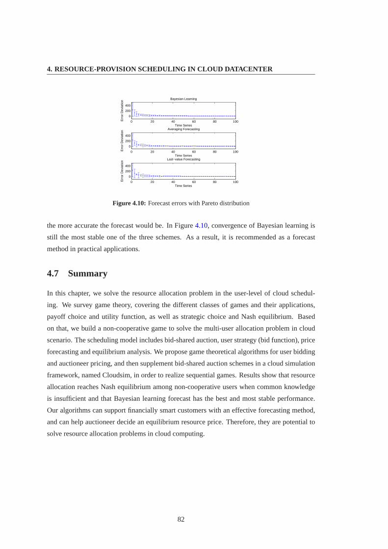
4. RESOURCE-PROVISION SCHEDULING IN CLOUD DATACENTER
0 20 40 60 80 100
0
200
400
Bayesian Learning
Time SeriesE
rror
Dev
iatio
n
0 20 40 60 80 100
0
200
400
Averaging Forecasting
Time Series
Err
or D
evia
tion
0 20 40 60 80 100
0
200
400
Last−value Forecasting
Time Series
Err
or D
evia
tion
Figure 4.10: Forecast errors with Pareto distribution
the more accurate the forecast would be. In Figure4.10, convergence of Bayesian learning is
still the most stable one of the three schemes. As a result, it is recommended as aforecast
method in practical applications.
4.7 Summary
In this chapter, we solve the resource allocation problem in the user-level ofcloud schedul-
ing. We survey game theory, covering the different classes of games and their applications,
payoff choice and utility function, as well as strategic choice and Nash equilibrium. Based
on that, we build a non-cooperative game to solve the multi-user allocation problemin cloud
scenario. The scheduling model includes bid-shared auction, user strategy (bid function), price
forecasting and equilibrium analysis. We propose game theoretical algorithms for user bidding
and auctioneer pricing, and then supplement bid-shared auction schemes in acloud simulation
framework, named Cloudsim, in order to realize sequential games. Results show that resource
allocation reaches Nash equilibrium among non-cooperative users when commonknowledge
is insufficient and that Bayesian learning forecast has the best and most stable performance.
Our algorithms can support financially smart customers with an effective forecasting method,
and can help auctioneer decide an equilibrium resource price. Therefore, they are potential to
solve resource allocation problems in cloud computing.
82

5
Real-time scheduling with MapReduce
in cloud datacenter
5.1 Introduction
Computing in clouds has become more instrumented, interconnected, intelligent and pervasive
than ever before. A cloud datacenter can carry out a wide spectrum ofdata-intensive applica-
tions to assist our daily activities and social problems, such as search indexing, mining social
networks, recommendation services and advertising back-ends. There are emerging classes of
cloud-based applications that benefit from increasing time guarantee. For example, real-time
advertising requires a real-time prediction about user intent based on their search histories.
Meeting deadlines here translates into higher profits for the content providers. In control dat-
acenter, enormous amount of real-time data should be collected and reportedperiodically by
various sensors. Besides that, ambient intelligence needs a networked database to integrate
these sensor data streams in time and to offer a real-time analysis according to event request .
Therefore, computing in clouds, where billions of events occur simultaneously, is not in time
linear dimension, but falls into the real-time computing category.
Real-time application is subject to a real-time constraint that must be met, regardless of
system load. If a real-time computation does not complete before its deadline, it is treated as a
failed case, as serious as that the computation is never executed. MapReduce [53] has emerged
as one of the most popular frameworks for distributed cloud computing. Dealing with different
real-time tasks on a MapReduce cluster can benefit users from sharing acommon large data
set. However, the traditional scheduling schemes need to be revised, in terms of particular
83
5. REAL-TIME SCHEDULING WITH MAPREDUCE IN CLOUD DATACENTER
characteristics of MapReduce.
MapReduce consists of two individual steps, inspired by Map and Reducefunctions. Firstly,
input data is chopped into smaller sub-problems, each of which runs a Map operation. After
all Maps finish, the intermediate answers of these sub-problems are assembled and then re-
assigned to Reduces according to different keys generated by Maps.Reduces only start after
all Maps are completed, which illustrates a special feature of MapReduce, that is, sequential
segmentation of task execution. The segmentation and interdependence betweenMap and Re-
duce, provide the primary motivation of our study on real-time scheduling on a MapReduce
cluster. In this chapter, we shall assume the computation ability of a cluster as a whole by
hiding assignment detail of every Map/Reduce task in the interior of the cluster.
The rest of this chapter is organized as follows. We first formulate the real-time scheduling
problem, based on which classical utilization bounds for schedulability test are revisited. Af-
ter analyzing the advantages and disadvantages of current utilization bounds, we then present
MapReduce scheduling model and a less pessimistic utilization bound, combining theparticu-
lar characteristics of MapReduce. Next we discuss scheduling performance of our mathemat-
ical model, following by experiment results implemented by SimMapReduce, a simulator of
MapReduce framework.
5.2 Real-time scheduling
We build a real-time scheduling problem model by a triple(Γ, P, A) whereΓ is the set of
real-time tasks,P the set of processing resources andA the scheduling algorithms.
5.2.1 Real-time task
A computing task is an application taking up memory space and execution time. The concept
of task should be distinguished from event. An event emphasizes an operation taking place at
a specific moment, while a task can be submitted, executed, halted, suspendedand returned.
For the purpose of time analysis, we define a real-time task by its timing characteristics,
rather than by the functionality requirements, such as execution time, lateness, deadline,etc.
The tasks to be scheduled make a task setΓ = {τ1, τ2, · · · , τn}, and anyτi consists of a
periodic sequence of requests. When a request arrives, a new instance is created. For the
periodic real-tasks, several preliminary terms should be defined.
84

5.2 Real-time scheduling
• Ti: period is the time between two successive instances of taskτi.
• Oi: offset is the first release of taskτi.
• Ci: computation time is the worst-case execution time ofτi.
• Di: deadline is the relative overdue time in one period.
In addition,τi,k denotes thekth instance ofτi. There are several important instants forτi,k,
and their relationship is shown in Figure5.1
• ai,k: activation instant at which instanceτi,k is released to the scheduler.
• si,k: starting instant at which the instanceτi,k starts computation.
• ei,k: execution time, it is how long instanceτi,k in running
• fi,k: finishing instant at which instanceτi,k finishes the execution.
• di,k: overdue instant at which instanceτi,k is required to be finished.
Figure 5.1: Relationship between important instants
All instances are activated after the request is submitted, soai,k is equal toOi + (k− 1)Ti.
The starting timesi,k can not be earlier than the activationai,k. The total amount of execution
time ei,k depends on the processing resources, but it can not exceed the worst execution time,
that isCi = max ei,k. The execution ofτi,k finishes atfi,k, andsi,k + ei,k ≤ fi,k. For most
cases, the equal sign is not true, because scheduler might execute morethan one task at the
same time. Finishing time is important but varies with different instances. Response time of
taskτi is defined as the maximum of finishing timeRi = max(fi,k − ai,k). The deadlinedi,k
is the absolute overdue time forτi,k, sodi,k = ai,k + Di. The task utilizationui = Ci/Ti
shows the impact of taskτi on processing resource. System utilization is the sum of allui, and
it presents the fraction of processor time used by periodic task set.
85

5. REAL-TIME SCHEDULING WITH MAPREDUCE IN CLOUD DATACENTER
U =n∑
i=1
ui (5.1)
Since the required amount of computation power can not exceed the availableresource, the
conditionU ≤ 1 must be satisfied if there are feasible scheduling solutions on task setΓ.
5.2.2 Processing resource
Processing resource is the resource in charge of executing tasks. Forthe sake of simplicity, we
distinguish processors one from another by its computing capability. The concrete processor
types or internal architectures are ignored in this model. Typical processing resources are
• Uniprocessor: there is only one processor in the set, and the worst-case computation time
depends on the size of executed tasks.
• Identical multiprocessor: the number of processors in set is more than one,and each of
them has the same computing capability.
• Uniform multiprocessor: the number of processors in set is more than one. Different
processors have different computing capability, but the speed on each processor is a
constant and does not depends on task type.
• Heterogeneous multiprocessor: multi processors are constituted by different hardware
platforms, so the worst-case computation time depends not only on task size, but also on
task type.
Among them, the uniprocessor and the identical multiprocessor are most studied, because
they are more general and easily analyzed than the multiprocessor of identicalor heterogeneous
configuration. The other two cases can be extended by identical multiprocessors. Especially,
many results achieved for the uniprocessor are useful for multiprocessor resources, we there-
fore focus the discussion on uniprocessor.
5.2.3 Scheduling algorithm
Scheduling algorithmA is the set of rules for mapping tasks fromΓ onto the processing re-
sourceP . An algorithm is preemptive if the execution of one task can be interrupted by another
task. The interrupted one is resumed later at the same location where the task was preempted.
86

5.2 Real-time scheduling
Non-preemptive algorithms are easily implemented because of no extra overhead needed for
context switch, but they can not promise that all deadlines are satisfied. Asa result, preemp-
tive algorithms are applied by real-time scheduling to handle applications with the stricttime
requirements.
Two basic constraints should be met. A task can not be executed on two or more processors
simultaneously, and a processor can not execute on two or more tasks. Under these premises,
a feasible scheduling algorithm is that the scheduling can make all tasks meet their deadlines.
An algorithm is optimal in the sense that no other feasible scheduling exists if the task set can
not be scheduled by this algorithm.
First In First Out (FIFO) algorithm queues tasks on a waiting list. When a new task is
submitted, scheduler puts it on the list according to its arrival time. Round-Robin (RR) is
another common scheduling algorithm. It handles all tasks without priority, and circularly
assigns a fixed time unit to each task in equal portions. However, both of themperform badly in
real-time scheduling system, which means they often fail to match the applications constraints.
In the context of real-time systems, the scheduling algorithm is priority driven. The tasks
are assigned priorities according to their constraints, and generally the highest priority is as-
signed to the most urgent task. When a task with low priority encounters another task with
high priority, the running one immediately hands over processor to the new task. Thus, the task
with the highest priority is always executed no matter whether the processoris occupied or not,
using preemption if necessary. In this case, a static scheduling algorithm refersto fixed priority
assignment. Once the priority is fixed, it never changes till the task is finished. Otherwise, the
scheduling algorithm is considered to be dynamic, if the priorities of tasks might change from
time to time. Although dynamic scheduling is more effective than static scheduling in utilizing
the available computational resources. Fixed priority assignment is more applied by industry
systems, owing to its efficient implementation, simplicity and intuitive meaning. For practical
purposes, we will focus on the study on static scheduling with fixed priority assignment.
5.2.4 Utilization bound
Utilization boundU provides a simple and practical way to test the schedulability of a real-
time tasks set. If the system utilization of a given task set∑
ui is lower than the boundU ,
the task set can be scheduled by processing resource. Although the bound is only sufficient,
not necessary, it is widely used in industry. Because it is easily implemented and fast enough
for on-line test. The simplest bound is decided by the number of tasks in task set. To raise
87

5. REAL-TIME SCHEDULING WITH MAPREDUCE IN CLOUD DATACENTER
system utilization bound, strict constrains are relaxed by subsequent researchers. The more
information of the task set included, the better the utilization bound obtained. In this section,
we revisit the development of utilization bound.
Classical bound
In 1973, Liu [82] proposed Rate Monotonic (RM) scheduling algorithm for preemptive periodic
tasks on uniprocessor in hard real-time system, which played seminal roles inthe development
of real-time scheduling research. RM algorithm assigns priorities to tasks inversely propor-
tional to their periods. Liu proved RM algorithm is the optimal fixed priority assignment, and
derived the lowest upper bound from the worst case of system utilization by arbitrary task set,
that is
U = n(21/n − 1) (5.2)
This bound decreases monotonically from 0.83 to 0.69 whenn approaches infinity. As
long as the utilization of a given task set is beneath this bound, schedulability is guaranteed.
However, this bound is only sufficient, not necessary. Many task sets withutilization higher
than this bound can still be scheduled. This phenomenon implies that the processing resource
is underutilized. The desire to improve the system utilization leads to research onmore precise
bound.
Closer period
Burchard [39] found an increasing utilization if all periods in a task set have values that are
close to each other. For a set ofn tasks, Burchard introduced two parametersSi = log2 Ti −⌊log2 Ti⌋ andβ = max Si −min Si. The least upper bound of processor utilization is
U =
{(n− 1)(2β/n−1 − 1) + 21−β − 1 β < 1− 1/n
n(21/n − 1) β ≥ 1− 1/n(5.3)
Higher utilization can be obtained if task periods satisfy certain constraintβ < 1 − 1/n.
The disadvantage is that more calculation is needed, such as searching forthe explicit task
periods.
88

5.2 Real-time scheduling
Harmonic chains
Appropriate choice of task periods guarantees high utilization, especially when task periods are
harmonic. Sha proved that schedulability is guaranteed up to 100% utilizaion with harnomic
periods [107]. The limitation of periods hedges the pratice in application domain. Kuo [75]
generalized this result by groupping tasks in serveral harmonic chains.Every harmonic chain is
a list of numbers in which every number divides every nunmber after it. If there arek harmonic
chains, clearlyk ≤ n, the least upper bound to processor utilization is
U = k(21/k − 1) (5.4)
A better bound is obtained by applying period parameters. However, determining the num-
ber of harmonic chains for a given task set also increases the time complexity.
Chen [49] investigated an exact bound that can be derived exhaustively underthe condition
where periods and computation times are integers. An algorithm withO(n3) complexity is
presented and performs better than harmonic bound. He also proposed another algorithm,
which yields an exact bound with exponential complexity.
Hyperbolic
Bini [32] proposed a schedulability condition similar to utilization bound. This condition does
not depend on the number of tasks. The schedulability test using Bini’s result has the same
complexity as using Liu’s bound, but less pessimistic. For a set ofn tasks with fixed priority
order, where each task is characterized by a single utilizationui, the task set is schedulable if
∏(ui + 1) ≤ 2 (5.5)
This result can also be integrated into the method of harmonic chains.
Two-level priority
Shih [108] proposed a semi-static scheduling algorithm. Two-level priority algorithm assign
tasks with two priorities, the low for old request and the high for deferred request. Deadline is
deferred if an instance of task does not finish before period expires,with maximum delay of
max(1, γ − 1), whereγ is the ratio between the longest period and the shortest period. The
least upper bound to processor utilization is
89

5. REAL-TIME SCHEDULING WITH MAPREDUCE IN CLOUD DATACENTER
U = [1 + n(21/n − 1)]/2 (5.6)
This bound approaches 0.845 whenn approaches infinity. However, this algorithm is not
optimal whenγ is greater than two.
Arbitrary deadline
A crucial assumption of RM algorithm is that the deadlineDi always equals periodTi. To better
utilize the processing resource, a heavily loaded resource chooses a relatively long artificial
deadline, while a lightly loaded resource applies a relatively short artificial deadline. In this
case, the deadlines may be different from the periods, and Liu’s bound breaks down.
Lehockzy [77] proposed an utilization bound for RM does not only depend on the number
of tasks but also the ratioδ = Di/Ti. When the number of tasks approaches infinity, the least
upper bound to processor utilization is
U =
δ δ ∈ [0, 12 ]
ln(2δ) + 1− δ δ ∈ [12 , 1]
2 ln( δ2S )− ln(δ − S) + 2S − 1 δ ∈ [1, 5
3 ]2 ln(3
4δ) + 2− δ δ ∈ [53 , 2]
(5.7)
WhereS is the smallest root ofS2 − (δ + 32)S + δ. The bound with arbitrary deadline
is a generalized expression of Liu’s bound. If one addition period is given, that isδ = 1, the
utilization bound increases from 0.69 to 0.81.
Aperiodic task
Some real-time systems contain tasks that have non-periodic requests, no fixed execution times
or no hard deadlines. Therefore, the periodic bounds are inapplicable without the periodicity
assumptions.
Abdelzaher [18] proposed a synthetic utilization in the spirit of Liu’s bound to test whether
the aperiodic tasks meet their deadlines. Synthetic utilization need information aboutthe com-
putation time and deadlines of all active tasks, that isU ξ =∑ Ci
Di. A active task means that
it has arrived, but has not yet expired. When the number of tasks approaches infinity, the least
upper bound to synthetic utilization is
U ξ = 2−√
2 (5.8)
90

5.3 Motivation from MapReduce
An arriving task that leadsU ξ to exceed the bound will be rejected. Consequently, aperiodic
utilization is improved by only accepting task whose deadline can be guaranteed.
5.3 Motivation from MapReduce
Besides sufficient tests with utilization bounds, there are several exact schedulability tests
yielding to sufficient and necessary conditions independently proposed by [78, 24, 111]. How-
ever, these exact tests are nearly intractable in real-time system. Their time complexity is
NP-hard for these non-trivial computational models [106], which is not acceptable for an on-
line test. We therefore concentrate on looking for a utilization bound on MapReduce cluster
for on-line schedulability analysis.
The improvement of bound is achieved by introducing practical requirementsof applica-
tions. When periodic tasks are executed on MapReduce cluster, the combinationof sequential
computing and parallel computing impacts on real-time scheduling. In the next section, we
analyze how the segmentation between Map and Reduce influences cluster utilization.
5.4 Real-time scheduling model for MapReduce tasks
5.4.1 System model
Assume a task setΓ = (τ1, τ2, · · · , τn) including n periodic tasks on MapReduce cluster.
Without losing generality, we letT1 < T2 < · · · < Tn. In RM scheduling, task with higher
request rate has higher priority, so taskτ1 with shortest period has highest priority, while the
last τn has the lowest. All tasks are independent, that is, have no precedence relationship.
Besides that, all tasks are fully preemptive, and the overhead of preemptive is negligible.
MapReduce solves distributable problems using a large number of computers, collectively
referred to as a cluster with certain computing capability. One task is partitioned intonm Maps
andnr Reduces. The numbers ofnm andnr are not fixed, varying from one task to another.
Maps performed in parallel finish in a certain timeMi, which means total time required to
completenm Map operations. Total time spent onnr Reduces is execution timeRi. For
simplification, we assumeRi is in proportion toMi, andα = Ri/Mi is introduced to express
the ratio between the two operations. Here we simply let all tasks use the sameα. The whole
computation time for taskτi is
91

5. REAL-TIME SCHEDULING WITH MAPREDUCE IN CLOUD DATACENTER
Ci = Mi + Ri = Mi + αMi =1
αRi + Ri (5.9)
One remarkable character of MapReduce is that no Reduce operation canbe submitted till
all Map operations finish, soMi andRi have innate temporal sequence and share no over-
lap. In the following context, we use Map/Reduce to signify the whole executing process of
Map/Reduce operations.
As former assumption, request of each instance occurs when a new period begins, so the
Map request is consistent with the request of the whole task. The moment when Reduce request
is submitted makes a huge impact on cluster utilization. If Reduce always executes as soon as
Map finishes, two stages of Map and Reduce are continuous. Hence the task can be considered
as a general case without segmentation, the bound of which is the famous Liu’sbound. If
Reduce does not make its request in a hurry, this tradeoff can be beneficial to cluster utilization
by making better use of spare time. We introduce parameterβ = TRi/TMi to reveal the
segmentation ratio. The sameβ is applied for all tasks in task setΓ. Clearly,
Ti = TMi + TRi = TMi + βTMi =1
βTRi + TRi (5.10)
Utilization ui is the ratio of computation time to its periodui = Ci/Ti. System utilization
U is the sum of utilization for all the tasks in task set.
U =n∑
i=1
ui =M1 + R1
T1+
M2 + R2
T2+ · · ·+ Mn + Rn
Tn(5.11)
5.4.2 Benefit from MapReduce segmentation
Seen from above system model, there is a natural segmentation between Map and Reduce.
For a MapReduce task, a delay might exist during the whole execution time, in contrast with
normal task executed in one go from beginning to end. How does this characteristic impact on
the schedulability performance? We take Figure5.2for example to give an intuitive idea.
There is a task setΓ = (τ1, τ2, τ3), in whichC1 = 4, C2 = 6. BecauseT1(12) < T2(16) <
T3(24), taskτ1 has the highest execution priority, while taskτ3 has the lowest.
Firstly, we analyze the case of normal tasks. In order to fully utilize cluster,the computation
timeC3 of taskτ3 is no more than 4. Otherwise, the cluster fails in scheduling these three tasks
simultaneously. In this case, the system utilization isUNormal = C1
T1+ C2
T2+ C3
T3= 0.875
92

5.4 Real-time scheduling model for MapReduce tasks
Figure 5.2: Comparison of normal task and MapReduce task
Next, we consider the case of MapReduce tasks withα = 1. Computation timeC3
can be increased to 7 from 4, without changingC1 andC2. The system utilization is then
UMapReduce = M1+R1
T1+ M2+R2
T2+ M1+R3
T3= 1.
Therefore, the system utilization augments owing to the segmentation between Map and
Reduce. Quantitative analysis of exact augmentation is presented in the nextsection.
5.4.3 Worst pattern for schedulable task set
At the beginning, let us review the concept of critical instant theorem proposed by Liu [82].
Theorem 1. A critical instant of a task is the moment at which the task makes a request which
has the largest response time. It happens whenever the task is requested simultaneously with
all higher priority tasks.
The concept implies the worst case occurs when all the tasks start to make requests at the
same time. Therefore, the offsets of all tasks are set to zero, that is,Oi = 0. In order to decide
whether a task set is schedulable, we check if and only if the first request of each task is met in
their first period when all tasks begin simultaneously.
In this section,TMi andTRi are treated as relative deadlines for Map and Reduce, respec-
tively. MapMi instantiates at the beginning of a new period, and must be finished beforeTMi .
At the momentTMi , ReduceRi makes the request, and its execution lasts forTRi at most. In
93

5. REAL-TIME SCHEDULING WITH MAPREDUCE IN CLOUD DATACENTER
this assumption, how does the cluster bound change according to the given latencyTMi? In
order to get the lowest utilization, we find out the worst pattern for schedulable task set on
MapReduce cluster. Lemma2 depicts the worst pattern for a schedulable task set that fully
utilizes MapReduce cluster.
Lemma 2. For a task setΓ = (τ1, τ2, · · · , τn) with fixed priority assignment whereTn >
Tn−1 > · · · > T2 > T1, if the relative deadline of Reduce is not longer than Map (β ≤ 1), the
worst pattern ensuring all tasks to be scheduled is
M1 = T2 − T1
M2 = T3 − T2
...
Mn−1 = 11+β Tn − Tn−1
Mn = (2 + α)T1 − 1+α1+β Tn
Proof. Suppose a task set fully utilizing MapReduce cluster. Fully utilizing has two meanings.
The first implies that a task set can be scheduled on cluster, and the second shows that no
improvement can be made in terms of cluster utilization. Each taskτi in task setΓ is defined
by a triple< Mi, Ri, Ti >, or equally< Mi, α, Ti > consideringα = Ri/Mi.
In order to analyze the period relationship between two neighboring tasks withthe most
adjacent priorities, we assume that
M1 = T2 −⌊
T2
T1
⌋· T1 + ǫ (5.12)
Whereǫ is a real number. We reduce Map runtimeM1 with ǫ whenǫ > 0. In order to
maintain the full processor utilization,Ma2 is improved with the amount ofǫ.
Ma1 = T2 −
⌊T2
T1
⌋· T1 T a
1 = T1
Ma2 = M2 + ǫ T a
2 = T2
......
Man = Mn T a
n = Tn
(5.13)
Through this adjustment cluster utilizationUa is consequently smaller than original uti-
lizationU , because
U − Ua = ǫ(1 + α)(1
T1− 1
T2) > 0 (5.14)
Although the two task sets fully utilize the cluster, the latter has a low cluster utilization.
As a result, the new pattern is worse than the former one.
94

5.4 Real-time scheduling model for MapReduce tasks
On the contrary, whenǫ < 0, M2 gets longer to fully use the cluster as
M b1 = T2 −
⌊T2
T1
⌋· T1 T b
1 = T1
M b2 = M2 +
⌈T2
T1
⌉· ǫ T b
2 = T2
......
M bn = Mn T b
n = Tn
(5.15)
The corresponding utilizationU b decreases again, owing to
U − U b = ǫ(1 + α)(1
T1−
⌈T2
T1
⌉1
T2) > 0 (5.16)
The worst pattern of task set makes cluster utilization reach minimum, as long asǫ ap-
proaches zero. The following analysis is based on the conditionǫ = 0.
Next, the periodT1 enlarges⌊
T2
T1
⌋times as
M c1 = T2 −
⌊T2
T1
⌋· T1 T c
1 =⌊
T2
T1
⌋· T1
M c2 = M2 + (
⌊T2
T1
⌋− 1)(T2 −
⌊T2
T1
⌋T1) T c
2 = T2
......
M cn = Mn T c
n = Tn
(5.17)
Compare new utilizationU c with U
U − U c = (1 + α)(1− 1/
⌊T2
T1
⌋)(
T2
T1) ≥ 0 (5.18)
This revise further pulls down the cluster utilization, which gives us inspirations that closer
periods degrade the system utilization. If we try to search for the worst pattern, the smallest
value of⌊
T c2
T c1
⌋should be taken. Hence the worst case happens when
⌊T c2
T c1
⌋= 1, in other words,
T2 < 2T1.
To sum up, we have
M1 = T2 − T1 (5.19)
Using similar methods, we obtain more results about the period relationship between two
adjacent tasks.
Mi = Ti+1 − Ti, i = 2, 3, · · · , n− 2 (5.20)
For the purpose of analyzing the relationship betweenTn−1 andTn, we construct a new task
95

5. REAL-TIME SCHEDULING WITH MAPREDUCE IN CLOUD DATACENTER
set by halving the periodTn−1. The periods of other tasks keep the sameT1, T2, · · ·Tn−2, Tn.
To avoid any waste, Map execution timeMn−1 is transferred fromτn−1 to τn.
Md1 = M1 T d
1 = T1
Md2 = M2 T d
2 = T2
......
Mdn−1 = 0 T d
n−1 = Tn−1/2
Mdn = Mn + Mn−1 T d
n = Tn
(5.21)
A lower utilizationUd is achieved, comparing with oldU
U − Ud = Mn−1(1
Tn−1− 1
Tn) > 0 (5.22)
The task set is resorted according to the length of period assuringTn > Tn−1 > · · · > T2 >
T1. The new pattern further decreases utilization under the condition thatT dn−1 < 1
1+β T dn ,
owing toT dn−1 ≤ 1
1+β · 2T dn−1 = 1
1+β Tn−1 < 11+β Tn = 1
1+β T dn .
MapMn−1 is obtained
Mn−1 =1
1 + βTn − Tn−1 (5.23)
Time left for Map executionMn is
Mn =1
1 + βTn −
n−1∑
i=1
Ci −n−1∑
i=1
Mi = (2 + α)T1 −1 + α
1 + βTn (5.24)
The above worst pattern stands for the most pessimistic situation where the leastutiliza-
tion can be calculated. Under the condition given by Lemma 2, schedulable upper bound on
MapReduce cluster is derived.
5.4.4 Generalized utilization bound
Theorem 3. For a task setΓ = (τ1, τ2, · · · , τn) with fixed priority assignment whereTn >
Tn−1 > · · · > T2 > T1, if the length of reduce is not longer than map (β ≤ 1), the schedulable
upper bound of cluster utilization isU = (1 + α){
n[(2+α1+β )1/n − 1] + β−α
1+β
}.
Proof. To simplify the notation, parametersγ1, γ2, · · · , γn are introduced
96
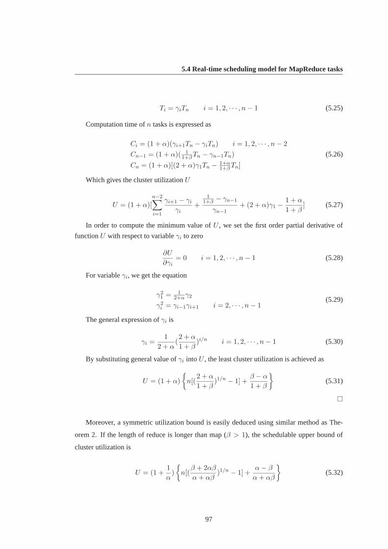
5.4 Real-time scheduling model for MapReduce tasks
Ti = γiTn i = 1, 2, · · · , n− 1 (5.25)
Computation time ofn tasks is expressed as
Ci = (1 + α)(γi+1Tn − γiTn) i = 1, 2, · · · , n− 2
Cn−1 = (1 + α)( 11+β Tn − γn−1Tn)
Cn = (1 + α)[(2 + α)γ1Tn − 1+α1+β Tn]
(5.26)
Which gives the cluster utilizationU
U = (1 + α)[n−2∑
i=1
γi+1 − γi
γi+
11+β − γn−1
γn−1+ (2 + α)γ1 −
1 + α
1 + β] (5.27)
In order to compute the minimum value ofU , we set the first order partial derivative of
functionU with respect to variableγi to zero
∂U
∂γi= 0 i = 1, 2, · · · , n− 1 (5.28)
For variableγi, we get the equation
γ21 = 1
2+αγ2
γ2i = γi−1γi+1 i = 2, · · · , n− 1
(5.29)
The general expression ofγi is
γi =1
2 + α(2 + α
1 + β)i/n i = 1, 2, · · · , n− 1 (5.30)
By substituting general value ofγi into U , the least cluster utilization is achieved as
U = (1 + α)
{n[(
2 + α
1 + β)1/n − 1] +
β − α
1 + β
}(5.31)
Moreover, a symmetric utilization bound is easily deduced using similar method as The-
orem 2. If the length of reduce is longer than map (β > 1), the schedulable upper bound of
cluster utilization is
U = (1 +1
α)
{n[(
β + 2αβ
α + αβ)1/n − 1] +
α− β
α + αβ
}(5.32)
97

5. REAL-TIME SCHEDULING WITH MAPREDUCE IN CLOUD DATACENTER
On a real MapReduce cluster, numerous tasks are executed concurrently, so the number
n is typically very large. Therefore, for all practical purposes, we aremost interested in the
cluster utilization asn→∞. Whenn is infinite, the limit ofU is
U∞ = limn→∞
U =
{(1 + α)[ln(2+α
1+β ) + β−α1+β ] β < 1
(1 + 1α)[ln(β+2αβ
α+αβ ) + α−βα+αβ ] β ≥ 1
(5.33)
5.5 Numerical analysis
Figure 5.3outlines the fluctuation of utilization bound with respect toα andβ, whereα shows
the proportion of execution time between Map and Reduce andβ illustrates the ratio between
two relative deadlines. Seen from Figure5.3, the bound is a symmetrical plane on the axis
α = β. It implies that the value ofα andβ should be harmonious, that is, difference between
α andβ can not be too dramatic. Easily understood, if a long Map (α < 1) is given a short
relative deadline (β > 1), it is impossible to schedule all the tasks before periods expire. That is
why the cluster utilization dips to zero when assignment of the two variables goesinto opposite
directions. Ifα andβ are given reasonable values in advance and task set can be scheduledon
MapReduce cluster, utilization bound is a concave function with respect toα andβ.
10−2
100
102
10−2
100
1020
0.2
0.4
0.6
0.8
1
β
Utilization w.r.t. α and β
α
Util
izat
ion
Figure 5.3: Utilization bound
In order to analyze the bound fluctuation more conveniently, we take three cross sections
of differentα. As shown in the Figure5.4, whetherα is greater, less than or equal to 1, the
bound first ascends, and then descends gradually. Cluster utilization reaches the highest point
atα = β.
98

5.5 Numerical analysis
10−1
100
101
0
0.1
0.2
0.3
0.4
0.5
0.6
0.7
0.8
0.9
1
β
\Util
izat
ion
Utilization w.r.t. β when α < 1 (α = 0.5)
β<1β>1u
10−1
100
101
0
0.1
0.2
0.3
0.4
0.5
0.6
0.7
0.8
0.9
1
β
\Util
izat
ion
Utilization w.r.t. β when α = 1
β<1β>1u
10−1
100
101
0
0.1
0.2
0.3
0.4
0.5
0.6
0.7
0.8
0.9
1
β
\Util
izat
ion
Utilization w.r.t. β when α > 1 (α = 2)
β<1β>1u
Figure 5.4: Utilization comparison with differentα
10−1
100
101
0
0.1
0.2
0.3
0.4
0.5
0.6
0.7
0.8
0.9
1
α
\Util
izat
ion
Utilization w.r.t. α when β < 1
β = 0.5
10−1
100
101
0
0.1
0.2
0.3
0.4
0.5
0.6
0.7
0.8
0.9
1
α
\Util
izat
ion
Utilization w.r.t. α when β = 1
β = 1
10−1
100
101
0
0.1
0.2
0.3
0.4
0.5
0.6
0.7
0.8
0.9
1
α
\Util
izat
ion
Utilization w.r.t. α when β > 1
β = 2
Figure 5.5: Utilization comparison with differentβ
Next we take three cross sections of differentβ using the same method. In Figure5.5,
a similar conclusion is summarized as the cases of fixedα. However, the curve is no longer
jumpy, but becomes smooth. Because the pessimistic bound is piecewise function with respect
to β, not toα. Another phenomenon that should be paid attention to is that the peak is not
necessarily reached at the pointα = β.
All these figures also suggest that the more harmoniousα andβ are, the more effective the
scheduling for a given task set could be. In order to find out where the maximum value ofU
is, we set the first order partial derivative of functionU with respect to variableβ to zero
(1 + α)(β − α) = 0 β ≤ 1
(1 + 1α)(β+1
β − α+1α ) = 0 β > 1
(5.34)
Both equations are true under the same conditionα = β. It is fair and in accord with
reality, that is, Map and Reduce share one period exactly according to their proportion.
U =
(1 + β)
{n[(2+β
1+β )1/n − 1]}
β < 1
(1 + 1β )
{n[(1+2β
1+β )1/n − 1]}
β ≥ 1(5.35)
Figure 5.6 is drawn whenα = β. The bound rises steadily due to segmentation of Map
99

5. REAL-TIME SCHEDULING WITH MAPREDUCE IN CLOUD DATACENTER
and Reduce. Whenβ approaches zero, the least cluster utilization is near 0.7. The amount of
utilization rises asβ goes up untilβ = 1, peaking at 0.81, which is also a global maximum
point. After that, cluster bound declines slowly to 0.7 again, whenβ increases to infinity.
10−2
10−1
100
101
102
0
0.1
0.2
0.3
0.4
0.5
0.6
0.7
0.8
0.9
1
β
Util
izat
ion
Utilization by Diagonal Slice
Segmented Request (α = β)Successive Request (LLB)
Figure 5.6: Optimal utilization
Notice that Liu’s utilization boundU = n(21
n − 1) can be represented in a task set with
β = 0 or β = ∞. β = 0 is an extreme case where the time spent on Reduce is negligible, so
Map execution time stands for the whole computation time. The case ofβ = ∞ implies that
Reduce execution occupies the whole computation time. Therefore, our new bound is a general
expression of Liu’s bound, only if a special value ofβ is assigned in these functions.
Our result improves the Liu’s work. This augmentation comes from the flexibility of
MapReduce. The execution of Map operations should be first promised, because Reduces
need to collect all the output of Maps. However, the moment when Reduce makes a request
changes the final cluster utilization. If Reduce waits in a reasonable period and hands over
cluster to a more pressing task with lower priority, it is possible to achieve more dynamic al-
location and a higher utilization bound than the case in which no segmentation exists between
Map and Reduce.
5.6 Evaluation
In order to further validate the effectiveness of the new scheduling algorithmfor MapReduce
tasks, we compare the proposed bound and Liu’s bound by a MapReduce simulator, named
SimMapReduce. SimMapReduce can model a vivid MapReduce environment and give a de-
tailed analysis on task processing. It supports multi-layer scheduling on user-level, job-level
100

5.6 Evaluation
Table 5.1: Node characteristics
Characteristics Parameters
Cluster rating 10000MIPS
memory 2G
storage 200G
bandwidth 100Mbps
network star-shaped
or task-level. For example, economic schemes coordinate demand and supply balance among
the users of MapReduce cluster, and heuristics dispatch Map/Reduce tasks to available CPUs.
Next, we complement the priority-based scheduling algorithms in SimMapReduce, andevalu-
ate the scheduling performance for real-time tasks in MapReduce cluster.
5.6.1 Simulation setup
We initialize .xml configure file as simulation setup.
(1) Setup of node: A MapReduce cluster is configured by homogeneousnodes. More
parameters are shown in Table5.1.
(2) Setup of user: A certain number of users enter into the cluster simultaneously. Any
userτi has an unique type of task, which arrives periodically. These periodic tasks construct a
sequence, belonging to one specific user.τi,k is thekth task in sequence. In this simulation,
the size of task sequence is 50. Users are given priorities by RM algorithm before simulation
starts, and these priorities are fixed throughout the execution of simulation. Thetask with short
period preempts the cluster whenever it meets task with long period. If any task is not finished
before the next task of the same user arrives, this task as well as its usercan not be scheduled
by the cluster. As a result, the set of tasks is not scheduable.
Two concepts concerning utilization should be clarified first. Task utilization isui = Ci/Ti,
and set utilization is the utilization sum of all types of tasksUΓ =∑
ui. Obviously,UΓ is no
more than one if there is a feasible scheduling algorithm. We then assume that one million
UΓ distribute uniformlyU(0, 1). For everyUΓ, a set of task utilizationui is generated by
Algorithm 3 [31].
Since this experiment only focuses on the computation time, data size including inputFile-
Size, intermediateFileSize, outputFileSize are set as small as possible. Especially, the time
101

5. REAL-TIME SCHEDULING WITH MAPREDUCE IN CLOUD DATACENTER
spent on data transmission approaches negligible compared with task executiontime, if the
bandwidth is large enough. The user characteristics are shown in Table5.2.
Table 5.2: User characteristics
Characteristics Parameters
set utilizationUΓ, [0,1]
user number 2, 20
task utilizationui uniform distribution [0, 1] (Algorithm 3)
task number 50
arrival intervalTi uniform distribution [10, 100]
MapTask length 10000 11+β uiTi (MI)
ReduceTask length 10000 β1+β uiTi (MI)
input size 1KB
intermediate size 1KB
output size 1KB
Algorithm 3 Generation of[u1, · · · , un] (JAVA)
1: n = 202: sumU = UΓ
3: for i = 1→ n− 1 do4: nextSumU = sumU ∗Math.pow(rand.nextDouble(), 1
n−i)5: ui = sumU − nextSumU6: sumU = nextSumU7: end for8: un = sumU
5.6.2 Validation results
For a givenUΓ, 1000 random sets are generated. Every setΓ = {τ1, τ2, · · · , τn} is examined
by bound test and simulation test. After repeated tests, an accepted ratio and asuccess ratio are
calculated with respect toUΓ.
If a MapReduce task is scheduled by classical Liu’s algorithm, Reduce stage begins imme-
diately after Map stage completes. The task is unscheduable if Reduce is finished after next
Map arrives.
102

5.6 Evaluation
In the new segmentation algorithm, two absolute deadlinesmDi,k andrDi,k are added for
MapTask and ReduceTask ofτi, respectively.
mDi,k = (k − 1)Ti + 11+β Ti
rDi,k = kTi(5.36)
MapTask is submitted when a new MapReduce task begins, and ReduceTask is submitted
at the momentmDi,k. The whole task is unscheduable, if MapTask is finished aftermDi,k or
if the ReduceTask is finished afterrDi,k. Consequently, theΓ = {τ1, τ2, · · · , τn} with UΓ can
not be scheduled on cluster.
0.5 0.6 0.7 0.8 0.9 10
0.1
0.2
0.3
0.4
0.5
0.6
0.7
0.8
0.9
1
UΓ
Acc
epte
d ra
tio
Bound test (2 tasks)
Liu
MR (β = 1)
MR (β = 0.5)
MR (β = 4)
Figure 5.7: Bound tests (2 tasks)
Figure5.7shows the accepted ratio of bound tests when the size of task set is two. These
tests seem like step functions. They thoroughly accept task set if the set utilization is less than
the bound, otherwise, refuse it. The MapReduce scheduling improves the classical bound in
varying extents, arriving at maximum whenβ equals one. Since these bounds are deduced
on the basis of worst cases, they are pessimistic for average case behaviors. As a result, it is
meaningful to lift bound for practical applications.
Figure5.8 shows the success ratios when there are 2 tasks in task set. Liu’s scheduling
is compared with the MapReduce algorithm whenβ equals 1, 0.5, 4, respectively. Our new
scheduling algorithm can promise better performance than original Liu’s method, because the
success ratio keeps on rising asβ approaches one. We take MapReduce scheduling withβ = 1
for example. When set utilization is less than 0.85, the schedulable probability for any ran-
dom set is 100%. This result has slight difference with the theoretical bound of 0.89, because
the transferring delay is included in simulated cluster, but ignored in the idealmodel. There-
103

5. REAL-TIME SCHEDULING WITH MAPREDUCE IN CLOUD DATACENTER
0.5 0.6 0.7 0.8 0.9 10
0.1
0.2
0.3
0.4
0.5
0.6
0.7
0.8
0.9
1
UΓ
Suc
cess
rat
io
Simulation (2 tasks)
Liu
MR (β = 1)
MR (β = 0.5)
MR (β = 4)
Figure 5.8: Simulation (2 tasks)
fore, this result can still validate the existence of the MapReduce bound proposed in previous
section, and further prove that the bound is only sufficient, not necessary. The schedulability
of a set under this bound is guaranteed, and the scheduability of a set beyond the bound is
uncertain. When set utilization is more than 0.85, there are still chances to schedule a set of
tasks on MapReduce cluster, but the propobility reduces with the increasing demand of cluster
utilization.
0.5 0.6 0.7 0.8 0.9 10
0.1
0.2
0.3
0.4
0.5
0.6
0.7
0.8
0.9
1
UΓ
Acc
epte
d ra
tio
Bound test (20 tasks)
LiuMR (β = 1)MR (β = 0.5)MR (β = 4)
Figure 5.9: Bound test (20 tasks)
Figure5.9shows the accepted ratios with 20 tasks in set. Similar conclusions can be made
as the case with 2 tasks. Liu’s bound is still the lowest, while the highest one is achieved by
MapReduce scheduling (β = 1). The bound ofβ = 0.5 performs better than theβ = 4,
becauseβ of the former is closer to one, the maximum value.
In Figure5.10, the differences of these algorithms are more obvious than that with 2 tasks.
104

5.7 Summary
0.5 0.6 0.7 0.8 0.9 10
0.1
0.2
0.3
0.4
0.5
0.6
0.7
0.8
0.9
1
UΓ
Suc
cess
rat
io
Simulation (20 tasks)
LiuMR (β = 1)MR (β = 0.5)MR (β = 4)
Figure 5.10: Simulation (20 tasks)
The sufficient threshold moves to 0.65 whenβ equals one, and to 0.55 when Liu’s algorithm
is taken. MapReduce scheduling is less pessimistic than Liu’s work, by upliftingthe real
schedulability. This improvement is determined by the property of MapReduce.The biggerβ
is, the more benefit is archived. Whenβ approaches zero, the two algorithms are nearly the
same.
5.7 Summary
In this chapter, we study the problem of scheduling real-time tasks on MapReduce cluster,
arising from demand for cloud computing. We first formulate the real-time scheduling problem,
based on which classical utilization bounds for schedulability test are revisited. We then present
a MapReduce scheduling algorithm, combining the particular characteristics of MapReduce.
After Map is finished, a proper pause before submission of Reduce canenhance scheduling
efficiency for the whole cluster. We deduce the relationship between clusterutilization bound
and the ratio of Map to Reduce. This new schedulable bound with segmentation uplifts Liu’s
bound. The latter can be further considered as a special case of the former. The effectiveness of
this bound is evaluated by simulation using SimMapReduce. Results show that this new bound
is less pessimistic, and it supports on-line schedulability test inO(1) time complexity.
105

5. REAL-TIME SCHEDULING WITH MAPREDUCE IN CLOUD DATACENTER
106

6
Reliability evaluation of schedulability
test in cloud datacenter
6.1 Introduction
Since real-time requirement is a significant QoS criterion of cloud service provision, schedula-
bility tests are necessary. These tests can determine whether an arriving application is accepted
or not, so it can well guarantee the system stability. Some of schedulability testsyield to
exact conditions to achieve the maximum system utilization, but the time complexity is not
acceptable for an on-line test. Some of them applying sufficient conditions mightsomewhat
underutilize cluster, but can be finished quickly, in predictable running time.Considering on-
line guarantee in clouds context, a test with constant-time complexity is more suitable for cloud
datacenter.
Although a number of constant-time tests have been studied, they are incomparable if the
determination conditions are different. In order to keep high system utilization, theproblem of
choosing a reliable test attracts our attention. Typically, simulation can give an intuitive answer,
but the result always depends on the way of generating random parameters and the number of
experiments. Therefore, we introduce a concept of test reliability to evaluate the probability
that a random task set can pass a given schedulability test, and define anindicator to express
the test reliability. The larger the probability is, the more reliable the test is. Fromthe point of
view of system, a test with high reliability can guarantee high system utilization.
The rest of this chapter is organized as follows. We first investigate the related research of
schedulability tests in real-time system. Then we explain the importance of on-line schedula-
107

6. RELIABILITY EVALUATION OF SCHEDULABILITY TEST IN CLOUDDATACENTER
bility tests in cloud datacenter, and present several related conditions for schedulability tests.
After introducing reliability indicator, we give some practicable examples to explain how the
indicator is used to compare the reliability of different tests. The comparison results are vali-
dated by SimMapReduce.
6.2 Schedulbility test
This chapter breaks the limitation that deadline exactly equals its period, and doesa general
survey on schedulability tests with arbitrary deadlines. In that case, DeadlineMonotonic (DM)
strategy replaces RM as the optimal priority assignment policy for periodic tasks [80]. Con-
sequently, assigned priorities are inversely proportional to the length of thedeadline. The task
with the shortest deadline is assigned the highest priority, while the one with the longest dead-
line has the lowest priority. When deadline equals period, DM assignment defaults to RM
assignment.
The schedulability test predicts temporal behavior of a given task set, anddecides whether
the deadline constraints will be met at runtime, that is, the given task set can bescheduled. Two
main types are
• Sufficient test: All task sets that pass the test can meet their deadlines. However, some
of task sets that do not pass the test can still be scheduled by processingresource.
• Exact test: A task set can be scheduled if and only if it passes the test.
In this chapter, we investigate current schedulability tests in terms of design principle,
time complexity and applicable scenario. System designers , who face a tradeoff between test
accuracy and overhead, could make a reasonable decision based on the available computational
power.
6.2.1 Pseudo-polynomial complexity
An exact schedulability test yields to a sufficient and necessary condition,but it requires high
computational complexity [70], even in the simple case where task relative deadlines are equal
to periods. Lehoczky [78] studied an exact feasibility test with pseudo-polynomial complexity
for that RM priority assignment. Based on linear programming, Park [98] achieved the exact
utilization bound without knowledge of exact task computation time. Subsequently, Audsley
108

6.2 Schedulbility test
[24] considered a DM priority assignment and improved Lehoczky’s exact feasibility test by
searching worst-case response time in an iterative manner. Lehoczky [77] then proposed a more
general feasibility test for arbitrary deadlines. Later, methods for speeding up the analysis of
task sets were proposed [87, 111, 17, 29, 49, 30], but the complexity of the approach always
remains pseudo-polynomial in the worst case. Here we present two seminal pseudo-polynomial
complexity tests.
Breakdown utilization
Breakdown utilization is first proposed by Lehoczky [78],describing an exact characterization
of RM scheduling algorithm. For a random task set, the computation time scales to the point at
which a deadline is first missed. The corresponding set utilization is the breakdown utilization
U∗n. This bound is an exact bound, which provides both sufficient and necessary conditions for
a schedulability test. If the utilization of task set is higher than this bound, no solution exists
for scheduling all the tasks on one processor. Otherwise, the task set can be scheduled with-
out missing any deadline. The result seems exciting, but this breakdown utilizationchanges
according to tasks with different periods and computation times. In other words, task set size
n is not enough to make a decision, and precise details such as computation timeCi, periodTi
for every task should be known in advance.
U∗n =
∑ni=1
Ci/Ti
mint∈Sn
∑nj=1
Cj⌈t/Tj⌉/t
Sn = kTj j = 1, · · · , n; k = 1, · · · , ⌊Tn/Tj⌋(6.1)
In order to characterize the average behavior, Lehoczky studied the asymptotic behavior
of the breakdown utilization when periods and computation times are generated randomly.
Especially,U∗n converges to a constant as the task set size increases, depending onlyon periods,
no longer on computation times. Given task periods generated uniformly in the theinterval
[1,B], breakdown utilizationU∗n converges to.
U∗n =
1 B = 1ln BB−1 1 < B < 2
ln BB
⌊B⌋+
∑⌊B⌋−1
i=21/i
B ≥ 2(6.2)
and the rate of convergence isO(√
n)
In addition, the function ofU∗n with respect toB first decreases and then increases asB
grows from one to infinity, bottoming atB = 2, which is in agreement with Liu’s result. For
109

6. RELIABILITY EVALUATION OF SCHEDULABILITY TEST IN CLOUDDATACENTER
uniformly distributed tasks, 0.88 is a reasonable approximation for the breakdown utilization
bound, which is much larger than Liu’s sufficient bound of 0.69.
Response time analysis
Breakdown utilization has a strict restriction that the deadline of a task must equalthe period.
For tasks with deadlines no more than periods, DM is the optimal priority assignment [80].
Audsley proposed a method to estimate the actual worst response time for each task, so the
schedulability test turns out to be a trivial comparison of each task’s response time and its
deadline.
Response time is the period between task submission and execution completion. Theworst
response timeRi for a taski equals the sum of its computation timeCi and the worst interfer-
enceIi. Interference is defined as the preemption time of higher priority tasks(j < i), and is
given by the sum of⌈
RiTj
⌉Cj .
Ri = Ci +∑
∀j<i
⌈Ri
Tj
⌉Cj (6.3)
Ri can be calculated by asymptotic iteration.
Rn+1i = Ci +
∑
∀j<i
⌈Rn
i
Tj
⌉Cj (6.4)
Rni is thenth iteration. The iteration begins atR0
i = 0, and ends atRn+1i = Rn
i . If
Rni reachesDi before termination of convergence, iteration also halts, that is to say, the task
set is not schedulable. This analysis intends to predict the worst interference that a task can
suffer from higher priority tasks. Since the prediction formulation does not refer to any priority
assignment strategy, it is effective for both RM and DM approaches.
6.2.2 Polynomial complexity
Response time analysis (RTA) is a popular method for schedulability analysis of real-time
tasks. Many efforts of RTA in the simplification have been made by reducing the number of
iterations [111, 38, 84]. Although some of them can shorten the run time with a saving of
26-33% calculation [84], all algorithms currently known still take runtime pseudo-polynomial
in the representation of the task system. Besides that, approximation is then appliedto further
reduce the time complexity of an exact schedulability test.
110

6.2 Schedulbility test
Fisher [58] derived a fully polynomial time approximation scheme of the RTA. This scheme
accepts two inputs, the specifications of a task system and a constantǫ ∈ [0, 1], to examine fea-
sibility tests. If the test returns feasible, the task set is guaranteed to be scheduled on the
processor for which it has been specified. If the test returns unfeasible, the task set is guaran-
teed to be unscheduled on a slower processor, the computing capacity of which is in (1 − ǫ)
proportion to the specified processor.
The number of iteration of interference calculation is limited to a constantk, wherek =
⌈1/ǫ⌉ − 1. So the approximated value ofIi is
Ii =
{ ⌈tTi
⌉Ci t ≤ (k − 1)Ti
Ci + tTi
Ci t > (k − 1)Ti
(6.5)
Therefore, the worst response timeRi is calculated inO(n2k) time complexity.
Ri = Ci +∑
∀j<i
Ii (6.6)
In addition, Bini [28] derived an upper bound on the response times in polynomial time.
The worst response timeRi is bounded byRubi as
Ri ≤Ci +
∑i−1j=1 Cj(1− Uj)
1−∑i−1j=1 Uj
= Rubi (6.7)
The time complexity of computing the response time upper boundRubi is O(i), and the
complexity of computing the bound for all the tasks isO(n2).
More polynomial complexity tests can apply the utilization bounds in the previous chapter.
For example, Han [64] suggested modifying the task set with smaller, but harmonic, periods
using an algorithm withO(n2 log n) complexity. Chen [49] investigated an algorithm with
O(n3) complexity that obtains an exact bound under the condition where periods and compu-
tation times are integers. Lauzac limited period relations, and improved schedulability within
aO(n log n) time complexity.
Generally speaking, all polynomial complexity tests are only sufficient, not necessary. The
time complexity for exact tests is always NP-hard for non-trivial computational models [106].
Less complexity is always achieved at the cost of less accuracy.
111

6. RELIABILITY EVALUATION OF SCHEDULABILITY TEST IN CLOUDDATACENTER
6.2.3 Constant complexity
The constant complexity tests apply the simplest bound, such as the classicalbound [82] or
the hyperbolic bound [32]. Both of these tests are inO(1) time complexity, so they are easily
implemented and fast enough for on-line schedulability tests. As long as the utilization of a
given task set is under this bound, all tasks can be scheduled for sure. One shortcoming is that
the two bounds are only suitable for RM approach. In order to find out a concise schedulable
condition like Liu’s result, Peng [99] proposed a concept of system hazard to check whether
assigned tasks miss their deadlines, and computed lowest upper bound of DMalgorithm. The
calculation of DM bound can be finished inO(1) time complexity.
Recently, another schedulability test withO(1) constant complexity has been developed by
Masrur [89, 88]. This test calculates an upper bound of the worst response time considering
all accepted tasks, and is different from all mentioned tests based system utilization. If this
upper bound does not exceed the respective deadlines, all tasks can be scheduled under DM.
However, the comparison with other bound-based tests remains unfinishedby the authors.
6.3 Motivation from constant complexity
In cloud computing, a service request may arrive at any time in a datacenter.In order to
guarantee the system against overload and collapse, an arriving task needs then to be admitted
or rejected on-line according to whether it can be feasibly scheduled withoutdisturbing other
tasks. Therefore, the datacenter requires a schedulability test that canbe finished in predictable
running time.
Schedulability tests strongly affect system stability, especially for system executing pe-
riodic tasks that treat deadline as a dominant QoS constraint. For example, each packet of
interactive computer games needs to be processed well before the arrival of the next packet.
From a practical point of view, we limit our study to fixed priority scheduling, because it is
prevailingly supported by commercial real-time operating systems.
Exact schedulability tests are already known for fixed priorities. Although high accuracy is
always desirable, exact tests are often not eligible for on-line requirement.The running time of
such a pseudo-polynomial test depends on various task parameters, sois difficult to precisely
bound such a running time in an on-line setting where the task set is constantly changing.
Polynomial-time approximation tests require tasks to be sorted according to decreasing
priority. When a new task arrives, we only need to add it to a sorted list, andthen retest all
112

6.4 On-line schedulability test
already accepted lower-priority tasks. This leads to additional delay and maybe impractical,
particularly, for a large number of tasks.
Considering the on-line nature of the problem in cloud computing, a schedulabilitytest
with constant time complexity is applicable, which does not depend on the numberof tasks
currently running in the system. Although there have been several candidates providing on-line
commitments, schedulability tests using different conditions are incomparable. The question
how to choose the best among all available alternatives provides the primarymotivation of our
study.
However, a criterion has not been established to compare the constant-time admission con-
trol test using different conditions. In this chapter, we introduce a method tocompare the
accuracy of different schedulability tests. The principle comes from the phenomenon that a
test admitting more tasks is more reliable given a number of random tasks. The reliability in-
dicator can be used to evaluate test performance. From the point of view of system, a test with
high reliability can guarantee high system utilization.
6.4 On-line schedulability test
We first clarify system model and relative terms that will appear in the following sections.
6.4.1 System model
A task setΓ = (τ1, τ2, · · · , τn) is formulated includingn independent periodic tasks. Taskτi
consists of a periodic sequence of requests. The interval between two successive instances is
periodTi. The time taken to executeτi is Ci. In the duration of any instance, computation must
be completed before the deadlineDi. Herein, we assumeCi ≤ Di ≤ Ti. Utilization ui is the
ratio of computation time to its periodui = Ci/Ti.
A task τi is schedulable with respect to an algorithm if no instance misses its deadline,
and a task setΓ is feasible with respect to an algorithm that can schedule all tasks in the set
before their deadlines. Each task is assigned to a priority before execution. Concrete priority
assignment is discussed in the next section. When a running task with lower priority encounters
a new request from a task with high priority, it hands over the cluster to the new instance with
a negligible overhead.
113

6. RELIABILITY EVALUATION OF SCHEDULABILITY TEST IN CLOUDDATACENTER
6.4.2 Test conditions
Liu’s RM condition
RM scheduling is an optimum static algorithm [82]. If RM can not make a task set schedulable
on a cluster, no other rules can succeed in scheduling. RM algorithm is only suitable for
the cases in which task period exactly equals its deadline. Liu proposed a concept of system
utilizationU as a sufficient condition for schedulability test. The subscriptsl, p andm represent
the work of Liu, Peng and Masrur detailed in the following content, respectively.
Theorem 4. For a set ofn tasks with fixed utilizationu1, u2, · · · , un, there exists a feasible
algorithm ensuring all tasks can be scheduled on a cluster if
Ul =n∑
i=1
ui ≤ n(21/n − 1) (6.8)
Peng’s DM condition
Deadline replaces period as the new determinant when deadline does not equal period. Peng
[99] modified the system utilizationUp for DM algorithm by introducing system hazardθ =
Di/Ti, 1 ≤ i ≤ n.
Theorem 5. For a set ofn tasks with fixed utilizationu1, u2, · · · , un, there exists a feasible
algorithm ensuring all tasks can be scheduled on a cluster if
Up =n∑
i=1
ui ≤{
θ θ ∈ [0, 0.5)
n[(2θ)1/n − 1] + 1− θ θ ∈ [0.5, 1](6.9)
Marur’s DM condition
Marsur [89] also studied a set of tasks with deadline no longer than period, and proposed a load
condition to test whether a task set is schedulable on a cluster.
Theorem 6. For a set ofn tasks with fixed utilizationu1, u2, · · · , un, there exists a feasible
algorithm ensuring all tasks can be scheduled on a cluster if
n∑
i=1
max(ui
θ,
2ui
1 + ui) ≤ 1 (6.10)
114
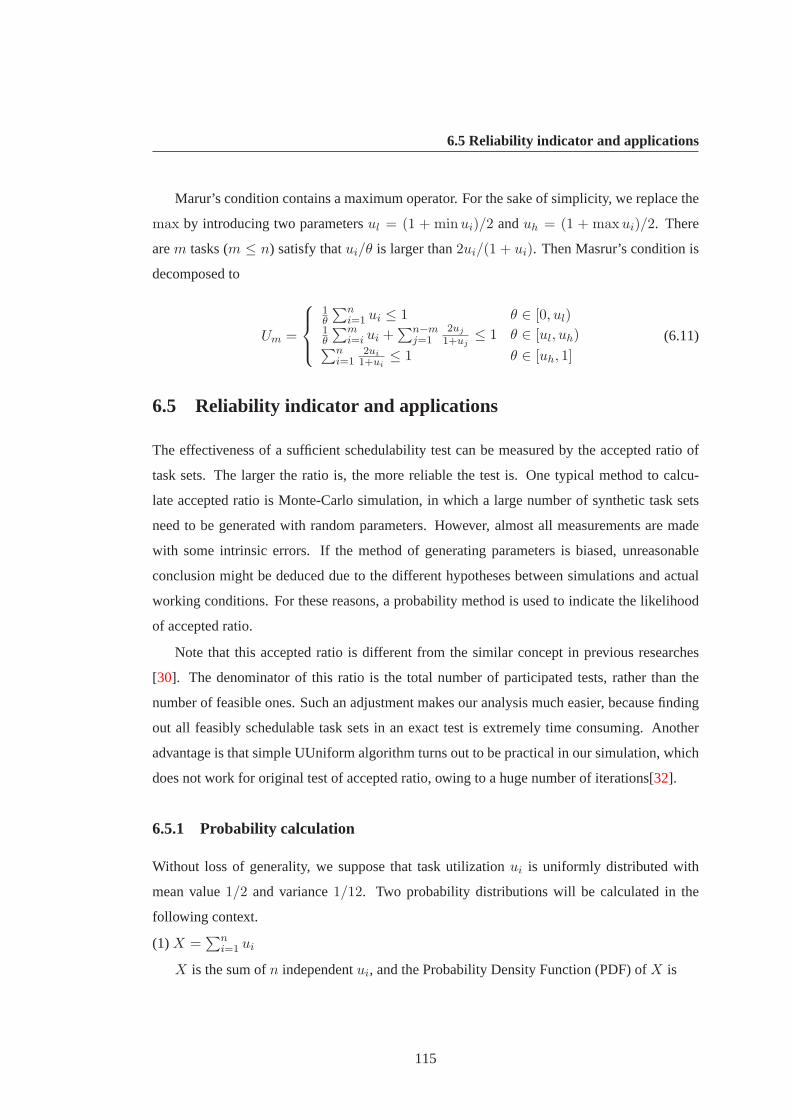
6.5 Reliability indicator and applications
Marur’s condition contains a maximum operator. For the sake of simplicity, we replace the
max by introducing two parametersul = (1 + minui)/2 anduh = (1 + maxui)/2. There
arem tasks (m ≤ n) satisfy thatui/θ is larger than2ui/(1 + ui). Then Masrur’s condition is
decomposed to
Um =
1θ
∑ni=1 ui ≤ 1 θ ∈ [0, ul)
1θ
∑mi=i ui +
∑n−mj=1
2uj
1+uj≤ 1 θ ∈ [ul, uh)∑n
i=12ui
1+ui≤ 1 θ ∈ [uh, 1]
(6.11)
6.5 Reliability indicator and applications
The effectiveness of a sufficient schedulability test can be measured by the accepted ratio of
task sets. The larger the ratio is, the more reliable the test is. One typical methodto calcu-
late accepted ratio is Monte-Carlo simulation, in which a large number of synthetic task sets
need to be generated with random parameters. However, almost all measurements are made
with some intrinsic errors. If the method of generating parameters is biased, unreasonable
conclusion might be deduced due to the different hypotheses between simulations and actual
working conditions. For these reasons, a probability method is used to indicatethe likelihood
of accepted ratio.
Note that this accepted ratio is different from the similar concept in previousresearches
[30]. The denominator of this ratio is the total number of participated tests, rather than the
number of feasible ones. Such an adjustment makes our analysis much easier, because finding
out all feasibly schedulable task sets in an exact test is extremely time consuming. Another
advantage is that simple UUniform algorithm turns out to be practical in our simulation, which
does not work for original test of accepted ratio, owing to a huge number of iterations[32].
6.5.1 Probability calculation
Without loss of generality, we suppose that task utilizationui is uniformly distributed with
mean value1/2 and variance1/12. Two probability distributions will be calculated in the
following context.
(1) X =∑n
i=1 ui
X is the sum ofn independentui, and the Probability Density Function (PDF) ofX is
115

6. RELIABILITY EVALUATION OF SCHEDULABILITY TEST IN CLOUDDATACENTER
FPDF (X) =1
(n− 1)!
⌊U⌋∑
k=0
(−1)k(nk)(U − k)n−1 U ∈ [0, n] (6.12)
Therefore,U has mean valuen/2 and variancen/12. Its Cumulative Distribution Function
(CDF) is
FCDF (X) =1
n!
⌊U⌋∑
k=0
(−1)k(nk)(U − k)n U ∈ [0, n] (6.13)
More generally, for a sequence of independent and identically distributed random variables
ui with expected valuesµ and variancesσ2, the central limit theorem asserts that for largen,
the distribution of the sumX is approximately normal with meannµ and variancenσ2.
X → N(n
2,
n
12) (6.14)
(2) Y =∑n
i=1 2ui/(1 + ui)
An intermediate variableyi = 1/(1 + ui) is introduced, and its PDF is expressed as
GPDF (yi) =1
y2i
yi ∈ [1
2, 1] (6.15)
Mean and variance ofyi are
E(yi) =
∫ 1
1
2
yig(yi)dyi = ln 2 (6.16)
D(yi) = E(y2i )− [E(yi)]
2 =1
2− (ln 2)2 (6.17)
With yi, we obtain
Y =n∑
i=1
2ui
1 + ui=
n∑
i=1
2(1− yi) (6.18)
Y is approximated by a normal distribution as
Y → N[2n(1− ln 2), 4n(1
2− (ln 2)2)] (6.19)
116

6.5 Reliability indicator and applications
6.5.2 Reliability indicator w
We define reliability indicatorw as
w =x− µ
σ(6.20)
For a generic normal random variable with meanµ and varianceσ2, the CDF isF (x) =
Φ(x−µσ ), in whichΦ(x) is the standard normal distribution. Since the CDF ofΦ(w) is a mono-
tone increasing function with respect tow, w can indicate the probability that a random task set
passes a given examination. The higher the probability is obtained, the better the examination
is. Therefore, different schedulability tests can be compared by a reliability indicator. The test
with a large value ofw is more reliable than that with a small value.
6.5.3 Reliability comparison of RM conditions
When deadline equals period, we have two RM sufficient conditions for schedulability test.
Based on Liu’s condition (6.8) and (6.14), we getµ = n/2, σ =√
n/12 andx = n(21/n−1), hence the reliability indicator of Liu’s condition is
wl =x− µ
σ=
n(21/n − 1)− n2√
n12
(6.21)
According to Masrur’s load test, we obtain
Um =n∑
i=1
2ui
1 + ui≤ 1 (6.22)
From (6.19), µ = 2n(1 − ln 2), σ =√
4n(12 − (ln 2)2) and x = 1, so the reliability
indicator of Masrur’s condition is
wm =x− µ
σ=
1− 2n(1− ln 2)√4n(1
2 − (ln 2)2)(6.23)
The comparison between the two reliability indicators has been plotted in Figure6.1. No-
tice thatwl is always larger thanwm, which implies that the schedulability test using Liu’s
condition is more reliable than that using Masrur’s condition. This comparison result can be
more intuitive when we focus on the accepted probability of the two tests.
117

6. RELIABILITY EVALUATION OF SCHEDULABILITY TEST IN CLOUDDATACENTER
2 4 6 8 10 12 14 16 18 20−9
−8
−7
−6
−5
−4
−3
−2
−1
0
Number of tasks
w
liumasrur
Figure 6.1: Comparison of reliability indicators
2 4 6 8 10 12 14 16 18 200
0.05
0.1
0.15
0.2
0.25
0.3
0.35
Number of tasks
Pro
babi
lity
liumasrur
Figure 6.2: Comparison of accepted probabilities
Figure6.2 shows the comparison of accepted probability with different numbers of tasks,
ranging from 2 to 20. Masrur’s test is more pessimistic, because an arbitrary task set has
lower probability of succeeding in Masrur’s test than in Liu’s test. The difference between
two accepted ratios diminishes as the number of tasks augments. When the number reaches a
certain value, the reliability of two tests is nearly the same. In Figure6.1 and Figure6.2, the
gap between two reliability indicators increases when the gap between accepted possibility is
reduced. Hence, the reliability indicator can only show relative differenceof test reliability,
rather than absolute performance.
118

6.5 Reliability indicator and applications
6.5.4 Reliability comparison of DM conditions
Next, the limitation that deadline exactly equals period is broken. In DM scheduling,we also
analyze two schedulable conditions when deadline is not longer than period.
According to Peng’s condition (6.9) and (6.14), we obtainµ = n/2, σ =√
n/12. Relia-
bility indicator is
wp =
θ−n2√n12
θ ∈ [0, 0.5)
n[(2θ)1/n−1]+1−θ−n2√
n12
θ ∈ [0.5, 1](6.24)
wp is a function of two variables ofn andθ, and its gradient vector is
∇wp(n, θ) = (∂wp
∂n,∂wp
∂θ) (6.25)
The gradient vector implies: (a)∂wp
∂n < 0 means that reliability indicator decreases as the
number of tasks increases. This result makes sense, because it is true that the schedulable
probability descends if more tasks try to enter cluster. (b)∂wp
∂θ > 0 means that the indicator
rises when the deadline is prolonged.
A factorα is introduced to represent the ratioα = m/n, and the distribution ofUm can be
developed as
Um →
N(µ1, σ21) θ ∈ [0, ul)
N(µ2, σ22) θ ∈ [ul, uh)
N(µ3, σ23) θ ∈ [uh, 1]
where:µ1 = 1
θn2
σ1 = 1θ
√n12
µ2 = αθ
n2 + 2(1− α)n(1− ln 2)
σ2 =√
αθ2
n12 + 4(1− α)n(1
2 − (ln 2)2)
µ3 = 2n(1− ln 2)
σ3 =√
4n(12 − (ln 2)2)
(6.26)
Reliability indicators are
wi =1− µi
σii = 1, 2, 3 (6.27)
Gradient vectors are
119

6. RELIABILITY EVALUATION OF SCHEDULABILITY TEST IN CLOUDDATACENTER
∇w1(n, θ) = (∂w1
∂n , ∂w1
∂θ )
∇w2(n, θ, α) = (∂w2
∂n , ∂w2
∂θ , ∂w2
∂α )
∇w3(n) = ∂w3
∂n
(6.28)
Reliability indicator of Masrur’s DM condition is quite complicated. (a)∂wi∂n < 0, i ∈
[1, 2, 3] shows that the accepted ratio of test decreases as the number of tasks increases. (b)∂w1(n,θ)
∂θ > 0 implies that lengthened deadline can increase the passing probability if the dead-
line is less than half of the period. (c) The variations ofw2(n, θ, α) in theθ andα directions are
not monotonic any more. Figure6.3shows how the value ofw2(n, θ, α) changes with respect
to θ andα.
0.60.8
1
0
0.5
1−1.5
−1
−0.5
0
θ
2 tasks
α
w
0.60.8
1
0
0.5
1−3.5
−3
−2.5
−2
θ
5 tasks
α
w
0.60.8
1
0
0.5
1−9
−8
−7
−6
θ
20 tasks
α
w
0.60.8
1
0
0.5
1−22
−20
−18
−16
θ
100 tasks
α
w
Figure 6.3: w2(n, θ, α) w.r.t θ andα
Reliability indicators of the two conditions are both piecewise functions. In orderto clearly
compare them, a factor is defined as
∆ = wm − wp (6.29)
The positive value of∆ indicates that a task set is more likely to pass Masrur’s test than
Peng’s test. In other words, Masrur’s test is better. Comparison can bedetailed by the following
four steps.
θ ∈ [0, 0.5)
∆1 = w1 − wp = 0 (6.30)
120

6.5 Reliability indicator and applications
In this part, the value of∆ is always zero, so two tests have the same reliability. System
designer can choose any of them as the schedulable condition.
θ ∈ [0.5, ul)
∆2 = w1 − wp (6.31)
Consideringn · minui ≤∑n
i=1 ui ≤ θ, another conditionθ < ul = (1 + minui)/2 <
(1 + θn)/2 is obtained. Therefore, the value ofθ falls into range[0.5, n/(2n− 1)).
0.50.6
0.70.8
0.91
0
5
10
15
200
0.01
0.02
0.03
0.04
0.05
0.06
θn tasks
∆(w
)
Figure 6.4: Better performance of Masrur’s test(θ ∈ [0.5, ul))
Figure6.4 presents the cases in which Masrur’s condition is less pessimistic than Peng’s.
When the deadline is relatively short, Masrur’s test performs better. However, this superi-
ority diminishes as more tasks admit in the system. That is caused by the possible field
[0.5, n/2n− 1) shrinks with increasing number of tasks.
θ ∈ [ul, uh)
∆3 = w2 − wp (6.32)
Figure6.5shows the performance comparison ifθ locates in the field[ul, uh). The points
on each sub-figure stand for the cases where Masrur’s condition exceeds the Peng’s. Especially,
Masrur’s test is more reliable for most cases when there are only two tasksin the set. Bursting
number of tasks results in the degradation of Masrur’s advantage.
The reliability indicator is not only useful for performance comparison, but also capable
of specifying an exact pattern where the winner can be applied. For example, in Figure6.5,
system designer can choose dominated condition based on foreseeablen, α andβ. If the point
appears on the figure, Masrur’s condition wins, otherwise, Peng’s testis preferred.
121

6. RELIABILITY EVALUATION OF SCHEDULABILITY TEST IN CLOUDDATACENTER
0.40.6
0.81
0
0.5
10
0.2
0.4
0.6
0.8
θ
2 tasks
α
∆(w
)
0.40.6
0.81
0
0.5
10
0.1
0.2
0.3
0.4
θ
5 tasks
α
∆(w
)
0.40.6
0.81
0
0.5
10
0.05
0.1
0.15
0.2
0.25
θ
20 tasks
α
∆(w
)
0.40.6
0.81
0
0.5
10
0.02
0.04
0.06
0.08
θ
100 tasks
α
∆(w
)
Figure 6.5: Better performance of Masrur’s test(θ ∈ [ul, uh))
θ ∈ [uh, 1]
∆4 = w3 − wp (6.33)
In this part, one condition needs to be satisfied, that is,θ > uh = (1 + maxui)/2 >
(1 + θn)/2. The possible field ofθ is [n/(2n− 1), 1].
0.50.6
0.70.8
0.91
0
5
10
15
200
0.1
0.2
0.3
0.4
θn tasks
∆(w
)
Figure 6.6: Better performance of Masrur’s test(θ ∈ [uh, 1])
In Figure6.6, only two short lines appear, which stand for the cases where Masrur’stest
performs better. Clearly, it seldom works as the dominated condition for schedulability test,
only under strict constraint that the number of tasks is no more than three. Hence Masrur’s
condition is not recommended to system designers.
122

6.6 Evaluation
6.5.5 Revisit of Masrur’s condition
It is interesting to notice the contradiction between our results and previous literature [89]. The
authors proved Marsur’s test is always less pessimistic than hyperbolic bound [32] and Liu’s
bound [82], if θ ∈ [0, ul). In our analysis of part 1 and 2, Masrur’s test sometimes performs
well, but not always.
In Masrur’s work [89], the Liu’s condition developed for RM is adapted to come up with
DM tests as
n∑
i=1
ui
θ≤ n(21/n − 1) θ ∈ [0, 1] (6.34)
However, this adoption is not true. Suppose there is a RM task setΓ1 with periodPi and
computation timeCi. Equation (6.34) is the test condition for another RM task setΓ2 with
periodθPi and computation timeCi, rather than for DM task setΓ3 with periodPi, deadline
θPi and computation timeCi.
The contradiction is caused by misunderstanding that Liu’s condition can be extended in
deadline monotonic algorithm. Equation (6.34) is not a DM condition for schedulability test.
The right test condition forΓ3 is (6.9). Therefore, the argument [89] is incomplete.
In the next section, we rectify this incorrect claim by extensive simulation amongdifferent
schedulability tests.
6.6 Evaluation
We use SimMapReduce to simulate a set of real-time tasks running on a MapReduce clus-
ter. Simple priority-based scheduling is applied in the following experiments. The priority
assignments are distinguished by rate monotonic and deadline monotonic algorithms.
Similarly as Chapter 5, the MapReduce cluster and the users are configuredin Table6.1
and Table6.2.
HereUΓ is set utilization, which is the sum of task utilizationui. Ti is the interval between
two successive tasks of the same user. Every task must be finished before the arrival of its
successor, otherwise, the whole task set can not be scheduled on the cluster.
123

6. RELIABILITY EVALUATION OF SCHEDULABILITY TEST IN CLOUDDATACENTER
Table 6.1: Node characteristics
Characteristics Parameters
cluster rating 10000MIPS
memory 2G
storage 200G
bandwidth 100Mbps
network star-shaped
Table 6.2: User characteristics
Characteristics Parameters
set utilizationUΓ, uniform distribution [0,1]
system hazardθ 0.3, 0.6, 0.9
user number 2, 20
task utilizationui uniform distribution [0, 1] (Algorithm 3)
task number 50
arrival intervalTi uniform distribution [10, 100]
MapTask length 5000uiTi (MI)
ReduceTask length 5000uiTi (MI)
6.6.1 RM scheduling results
This experiment compares accepted ratio of schedulability tests with the probability that a ran-
dom task set can be scheduled. For the case of RM algorithm, schedulability tests apply Liu’s
and Masrur’s conditions, respectively. Concrete experimental process is shown in Algorithm
4.
For each value of set utilizationUΓ, we randomly generate 20 tasks. Each task utilization
distributed uniformly, and the sum ofui equalsUΓ. Other parameters are configured as Table
??. Then the task set passes Liu’s and Masrur’s schedulability tests, with results whether this
task set is accepted. After that, SimMapReduce runs the task set, and reports the final decision
whether these tasks can be scheduled on a real MapReduce cluster. Theaccepted ratio and exact
scheduled ratio can be calculated by a large number of task sets, so we repeat this examination
a thousand times with the same hypothetical assumptionUΓ.
Figure6.7shows accepted ratios with respect to set utilization. Since Liu’s test is decided
124

6.6 Evaluation
Algorithm 4 Reliability comparison of RM conditions(JAVA)
1: N = 202: numExp = 10003: UΓ
4: for i = 1→ numExp do5: generate[u1, · · · , uj , · · · , uN ] randomly6: configure other parameters of task set7: Liu’s schedulability test8: if passthen9: nLiu + +
10: end if11: Masrur’s schedulability test12: if passthen13: nMasrur + +14: end if15: SimMapReduce simulation16: if passthen17: nSim + +18: end if19: end for20: Liu’s accepted ratiopLiu = nLiu/numExp21: Masrur’s accepted ratiopMasrur = nMasrur/numExp22: Exact scheduled ratiopSim = nSim/numExp
0 0.2 0.4 0.6 0.8 10
0.1
0.2
0.3
0.4
0.5
0.6
0.7
0.8
0.9
1
UΓ
Acc
epte
d ra
tio
RM scheduling (20 tasks)
Liu boud testMasrur load testSimulation
Figure 6.7: RM conditions
by the set utilization, the schedulability curve looks like a sign function. When setutilization
is less than Liu’s bound, the accepted ratio is one, otherwise, it is zero. Masrur’s test can not
be compared with Liu’s directly, but experiment results illustrate that Masrur’s condition is
125

6. RELIABILITY EVALUATION OF SCHEDULABILITY TEST IN CLOUDDATACENTER
more pessimistic, which coincides with the result obtained by reliability indication method. In
addition, both tests are sufficient. Notice that a violation appears whenUΓ = 0.7. Liu’s test
predicts that any task set is schedulable, but simulation reveals that only 86%of task sets can
be scheduled on a MapReduce cluster. The reason is that file transmissionoccupies some time
in the MapReduce simulation. For a real-time task, a tiny delay is not permitted. For arandom
task set with utilization of more than 0.7, it is possible to be scheduled by the cluster, though
this probability reduces as set utilization increases.
6.6.2 DM scheduling results
When deadline is no longer than period, DM schedulability tests apply Peng’s and Masrur’s
conditions, respectively. The following experiments target on analyzing theschedulability with
respect to set utilizationUΓ and system hazardθ. The simulation flow is similar to that in RM
experiments, except that two parameters, set size and system hazard, vary their values.
Given a fixed system hazardθ, we first analyze the accepted ratio of schedulability tests
with respect to set utilizationUΓ. Concrete experimental process is shown in Algorithm 5.
We takeθ = 0.5 andN = 2 for example. Twenty one types of task sets are generated, and
their set utilizationsUΓ uniformly locate in the field[0, 1]. For anyUΓ, the same simulation is
repeated 1000 times, but given differentN tasks.
When the size of task set is two, schedulability analysis is shown in Figure6.8 and Fig-
ure 6.9. Generally,UΓ < θ is a necessary condition that a random task set can pass any
schedulability test.
Figure6.8deals with the accepted ratios with respect toUΓ, by varyingθ with the value of
0.5, 0.7 and 0.9. Masrur’s test is beneficial to the tasks with a large set utilization, by offering
more opportunities to enter a cluster. Takeθ = 0.9 for example, task set with 80% utilization
could be scheduled at 25% probability if system employs Masrur’s schedulability test, but
would certainly failed if Peng’s test in applied. Comparing three sub-figures in Figure6.8, the
benefit of Masrur’s test magnifies as the deadline is prolonged. However, this advantage is
obtained at the cost of reducing schedulable possibility for the tasks with small set utilization.
Figure6.9 deals with the accepted ratios with respect toθ, by varyingUΓ with the value
of 0.5, 0.7 and 0.9. Test performance, in terms of schedulable probability for a random task,
is interpreted as the area under the curve of accepted ratio. Two tests perform the same when
UΓ is less than 0.5. Peng’s test allows more tasks to enter the cluster whenUΓ equals 0.7,
while Masrur’s test still admits tasks when Peng’s refuses everything atUΓ = 0.9. These
126

6.6 Evaluation
Algorithm 5 Accepted ratio w.r.tUΓ
1: θ = 0.52: N = 23: numU = 214: numExp = 10005: for i = 1→ numU do6: UΓ = 0.05 ∗ (i− 1)7: for j = 1→ numExp do8: generate[u1, · · · , uk, · · · , uN ] randomly9: configure other parameters of task set
10: Peng’s schedulability test11: if passthen12: nPeng + +13: end if14: Masrur’s schedulability test15: if passthen16: nMasrur + +17: end if18: SimMapReduce simulation19: if passthen20: nSim + +21: end if22: end for23: Peng’s accepted ratiopPeng = nPeng/numExp24: Masrur’s accepted ratiopMasrur = nMasrur/numExp25: Exact scheduled ratiopSim = nSim/numExp26: end for
results exactly agree with the conclusion deduced by the reliability analysis. Although they are
very intuitive, they can not provide a practicable solution for system designers as the reliability
indication method does.
Next, we analyze the cases with 20 tasks per set in Figure6.10and Figure6.11. Obviously,
Peng’s test outperforms Masrur’s in any case. When the deadline is relatively short (θ = 0.5),
two tests have the same reliability.
In Figure6.10, Peng’s reliability keeps growing asθ increases from 0.5 to 0.9, while the
reliability of Masrur’s test remains almost unchanged. This phenomenon seems to go against
Masrur’s test being always better than Peng’s whenθ ∈ [0.5, ul). That is actually caused
by the small probability of preconditions. The possibility that task utilization is less than
ul is expressed asPr(ui < ul). According to multiplication rule, forn independent tasks,
127

6. RELIABILITY EVALUATION OF SCHEDULABILITY TEST IN CLOUDDATACENTER
(a)
0 0.2 0.4 0.6 0.8 10
0.1
0.2
0.3
0.4
0.5
0.6
0.7
0.8
0.9
1
UΓ
Acc
epte
d ra
tio
θ = 0.5 (2 tasks)
Peng boud testMasrur load testSimulation result
(b)
0 0.2 0.4 0.6 0.8 10
0.1
0.2
0.3
0.4
0.5
0.6
0.7
0.8
0.9
1
UΓ
Acc
epte
d ra
tio
θ = 0.7 (2 tasks)
Peng boud testMasrur load testSimulation result
(c)
0 0.2 0.4 0.6 0.8 10
0.1
0.2
0.3
0.4
0.5
0.6
0.7
0.8
0.9
1
UΓ
Acc
epte
d ra
tio
θ = 0.9 (2 tasks)
Peng boud testMasrur load testSimulation result
Figure 6.8: Accepted ratio w.r.t.UΓ (2 tasks)
(a)
0 0.2 0.4 0.6 0.8 10
0.1
0.2
0.3
0.4
0.5
0.6
0.7
0.8
0.9
1
θ
Acc
epte
d ra
tio
UΓ = 0.5 (2 tasks)
Peng boud testMasrur load testSimulation result
(b)
0 0.2 0.4 0.6 0.8 10
0.1
0.2
0.3
0.4
0.5
0.6
0.7
0.8
0.9
1
θ
Acc
epte
d ra
tio
UΓ = 0.7 (2 tasks)
Peng boud testMasrur load testSimulation result
(c)
0 0.2 0.4 0.6 0.8 10
0.1
0.2
0.3
0.4
0.5
0.6
0.7
0.8
0.9
1
θ
Acc
epte
d ra
tio
UΓ = 0.9 (2 tasks)
Peng boud testMasrur load testSimulation result
Figure 6.9: Accepted ratio w.r.t.θ (2 tasks)
the event that all utilizations are belowul occurs with the possibility∏
Pr(ui < ul). Since
0 < Pr(ui < ul) < 1, the product decreases sharply with a largen. Besides that,θ <
128

6.6 Evaluation
(a)
0 0.2 0.4 0.6 0.8 10
0.1
0.2
0.3
0.4
0.5
0.6
0.7
0.8
0.9
1
UΓ
Acc
epte
d ra
tio
θ = 0.5 (20 tasks)
Peng boud testMasrur load testSimulation result
(b)
0 0.2 0.4 0.6 0.8 10
0.1
0.2
0.3
0.4
0.5
0.6
0.7
0.8
0.9
1
UΓ
Acc
epte
d ra
tio
θ = 0.7 (20 tasks)
Peng boud testMasrur load testSimulation result
(c)
0 0.2 0.4 0.6 0.8 10
0.1
0.2
0.3
0.4
0.5
0.6
0.7
0.8
0.9
1
UΓ
Acc
epte
d ra
tio
θ = 0.9 (20 tasks)
Peng boud testMasrur load testSimulation result
Figure 6.10: Accepted ratio w.r.t.UΓ (20tasks)
(a)
0 0.2 0.4 0.6 0.8 10
0.1
0.2
0.3
0.4
0.5
0.6
0.7
0.8
0.9
1
θ
Acc
epte
d ra
tio
UΓ = 0.5 (20 tasks)
Peng boud testMasrur load testSimulation result
(b)
0 0.2 0.4 0.6 0.8 10
0.1
0.2
0.3
0.4
0.5
0.6
0.7
0.8
0.9
1
θ
Acc
epte
d ra
tio
UΓ = 0.7 (20 tasks)
Peng boud testMasrur load testSimulation result
(c)
0 0.2 0.4 0.6 0.8 10
0.1
0.2
0.3
0.4
0.5
0.6
0.7
0.8
0.9
1
θ
Acc
epte
d ra
tio
UΓ = 0.9 (20 tasks)
Peng boud testMasrur load testSimulation result
Figure 6.11: Accepted ratio w.r.t. θ (20tasks)
(1 + minui)/2 < (1 + θn)/2 must be met, so the value ofθ falls into range[0.5, n/(2n− 1)).
When the task numbern increases,n/(2n− 1) approaches 0.5 gradually.
129

6. RELIABILITY EVALUATION OF SCHEDULABILITY TEST IN CLOUDDATACENTER
As a result of transmission delay, the schedulable ratio is less than 100%, and does not fit
in with the schedulability tests exactly. However, the overall variation is accordance with the
reality. These experimental results further validate our reliability comparison of the two DM
schedulability test. Since it is rare that MapReduce cluster only deals with two tasks in reality,
Peng’s condition is more suitable for DM schedulability test than Masrur’s.
6.7 Summary
In this chapter, we contemplate real-time schedulability tests in cloud datacenter.The schedu-
lability tests aim at determining whether a set of tasks is schedulable on a cluster. Some of
them yield to exact conditions to achieve the maximum system utilization, but the time com-
plexity is not acceptable for on-line tests. Some of them applying sufficient conditions might
somewhat underutilize a cluster, but they can be executed in predictable running time. We
focus on the tests with constant-time complexity, because a schedulability test in cloud com-
puting should be taken on-line. Given the lack of general solutions to evaluate the accuracy
of schedulability tests, we propose a method to indicate test reliability. Througha reliability
indicator, the probability of passing different tests can be compared. We apply this method
in several classical schedulability tests. Results show that Liu’s salient bound is a dominated
condition in RM tests. For DM tests, test reliability depends on system parameters. If these pa-
rameters are known in advance, datacenter designers can analyze the performance exactly, and
then choose an applicable test among several alternatives. We also validated these conclusions
by simulation using SimMapReduce.
130

7
SimMapReduce: a simulator for
modeling MapReduce framework
7.1 Introduction
MapReduce is a language-independent framework proposed by Google, which targets on solv-
ing data explosion problem for real Internet services. As a parallel programming framework, it
organizes a large number of computers with relatively simple functional primitives. Although
MapReduce is simple, it is capable of solving many real world problems, especially the prob-
lems processing huge datasets such as data mining [133], scientific computing [55], artificial
intelligence [47], and image processing [92] etc. In most of these cases, programmers are free
from some tough tasks such as distributing data, specifying parallelism and fault tolerance, and
only need to implement two functions: Map and Reduce. That is the reason whyMapReduce
quickly evolves as a prominent and mainstream programming model for data processing in the
past couple of years.
More attentions are paid to MapReduce not only by IT enterprises, but alsoby research
institutes. The researchers make efforts on theoretical analysis on MapReduce computational
model [127], scheduling mechanisms [129, 132, 131], task assignment [120, 95], workflow
optimization, instead of implementing a real MapReduce application. In addition, different ap-
plications require different system configurations and parameters, so the construction of such
real MapReduce systems is extremely challenging on a large scale of infrastructures. Under
above considerations, simulation method becomes a good alternative, which can accelerate
study progress by opening the possibility of evaluating tests with hypothesis setting in advance
131

7. SIMMAPREDUCE: A SIMULATOR FOR MODELING MAPREDUCEFRAMEWORK
and by simplifying the programming of implementation. It is easy to configure the infrastruc-
tures according to user requirements, and costs very few to repeatedly test various performances
in a controllable manner.
Although there are some open source supporters of MapReduce implementation, few spe-
cific simulators exist to offer a simulated environment for MapReduce theoretical researchers.
Therefore, a simulation tool, SimMapReduce, is developed to simulate the performance of dif-
ferent applications and scenarios using MapReduce framework. The users of SimMapReduce
only concentrate on specific research issues without getting concerned about finer implemen-
tation details for diverse service models.
The rest of this chapter is organized as follows. We first investigates the parallel program-
ming model, MapReduce, including its language syntax, logical dataflow, related data storage
and current implementations. Targeting on assisting researchers by optimizing parameter con-
figuration and testing new theoretical algorithms, a simulator modeling MapReduce framework
is developed. Next, we present simulator design issues such as system architecture, implemen-
tation diagram and modeling process. More research values of SimMapReduce are explained
in the end of this chapter.
7.2 MapReduce review
7.2.1 Programming model
MapReduce is a programming model for executing distributed data-intensive computations on
clusters of commodity machines. It was originally developed by Google and adopted world-
wide via an open-source implementation called Hadoop. Today, a vibrant software ecosystem
has sprung up around Hadoop, with significant activities in both industry and academia.
MapReduce is the very successful abstraction over large-scale computational resources.
The abstraction is inspired by the Map and Reduce primitives in functional languages such as
Lisp, Haskell, etc. Map function is in charge of splitting input file into chops andprocessing
each of them to generate a set of intermediate pairs, while Reduce function attempts to merge
all intermediate values and makes the final result. By performing Map and Reduce operations
in parallel, MapReduce allows distributed processing on a large server farm.
The syntax of MapReduce model is
Map(key1, value1)→ list(key2, value2)Reduce(key2, list(value2))→ list(key3, value3)
(7.1)
132

7.2 MapReduce review
Key-value pairs form the basic data structure in MapReduce. Keys and values may be
primitives such as integers, strings or other complex structures. When a MapReduce program is
written, the key-value structure on arbitrary datasets should be imposed. Take web application
for instance, the keys can be URLs and values can be the actual HTML content.
The input of a MapReduce job is the data stored on the underlying distributedfile system.
Every chunk of input is expressed as a key/value pair. Map function is applied to every in-
put (key1, value1) pair to generate an arbitrary number of intermediate (key2, value2) pairs.
The Map phase ends till all input (key1, value1) pairs are processed. (key2, value2) pairs are
shuffled and sorted into several groups, where each group has the same key2. Then Reduce
function is applied to all values associated with the same intermediate key2 to generate output
(key3, value3) pairs. Output key/value pairs from each Reducer arewritten persistently back
onto the distributed file system. Figure7.1shows the logical dataflow of MapReduce.
Figure 7.1: Logical view of MapReduce model
Overall, the MapReduce procedure is informally described as five steps
• Read input data from file system
133

7. SIMMAPREDUCE: A SIMULATOR FOR MODELING MAPREDUCEFRAMEWORK
• Map: extract useful information from every data chunk
• Sort: aggregate values by keys
• Reduce: filter useful information and summarize the final results
• Write output data to file system
Note that the keys in Map and Reduce phase are not the same. The data form of key/value
pair is flexible, so that programmers are free to decide the keys in these two phases. There is
a slight difference between the Hadoop implementation of MapReduce and Google’s imple-
mentation. In Google’s MapReduce, the output key of Reduce function must be the same key
as input. However, the programmers of Hadoop are free to change the keys in Reducer, so an
arbitrary number of output key/value pairs is emitted.
Overall, a typical MapReduce computation processes terabytes of data on thousands of
machines, so the MapReduce tasks are more data-intensive, rather than compute-intensive. A
MapReduce framework can be compared with other similar computing paradigms.
• HPC: the HPC jobs run on a fixed number of machines communicate through a mech-
anism like MPI. MapReduce jobs are elastic, so we can change allocations over time.
HPC jobs are often CPU-bound, so there is less need for node-level datalocality. Espe-
cially for parallel computing with shared memory, the parallel tasks have close relation-
ship with each other. In MapReduce, every Mapper or Reducer deals with independent
subtasks on separated machines.
• Grids: Grid jobs are more compute-intensive than MapReduce. The distributed comput-
ing refers to an organization of geographic clusters, rather than a cluster of commodity
machines. Moreover, errors from one grid task does not affect the results of other tasks,
but in MapReduce the mistakes in Map phase will cause further mistakes in Reduce
phase, even a wrong final result.
• Parallel Databases: parallel databases run data-intensive workloadson a distributed sys-
tem. The main concerns differentiating MapReduce from these systems are the scalable
use of commodity hardware in MapReduce, and the MapReduce execution strategy of
small independent tasks instead of long-running pipelined queries.
134
7.2 MapReduce review
7.2.2 Distributed data storage
In traditional cluster architectures, storage is viewed as a separate component from computa-
tion. As dataset sizes increase, more computing capacity is required for processing. In that
case, the storage and the link between the compute nodes become a bottleneck.One feasi-
ble solution is breaking the separation of computation and storage as distinct components in
a cluster. MapReduce adopts distributed file system that underlies programming model to re-
alize parallel computations. Google File System (GFS) and Hadoop Distributed File System
(HDFS) are two implementation of distributed file system.
The main idea is to divide user data into blocks and to replicate those blocks across the
local disks of nodes in the cluster. The distributed file system adopts master-slave architecture
on which the master maintains the file namespace and the slaves manage the actualdata blocks.
An application wishing to read a file must contact the master to determine where the actual
data is stored. As response, master transfers metadata and the location where the block is held.
The application then retrieves data from the slaves that store the actual data. All data transfers
only occur between applications and slaves.
Master is responsible for maintaining metadata, directory structure, file to blockmapping,
location of blocks, and access permissions. These data are held in memory for fast access, and
all mutations are persistently logged. Master ensures the integrity of the system.It decides
where the data replicas are created to keep the fault tolerance and systembalancing.
7.2.3 Hadoop implementation framework
MapReduce is applied to large datasets as a reliable and distributed computing paradigm to
process tera- or petabytes data in parallel. One key characteristic is that itinterleaves sequential
and parallel computation. On the parallel part, all computations are executed in parallel either
in Map phase or in Reduce phase. On the part of sequential process, Map is always taken before
Reduce, because Reduce should wait for the results integrated by the output of all Maps.
Google’s MapReduce implementation is roughly based on the above idea, but ispatented
privacy [53]. However, Google published a paper to describe technical details of theimple-
mentation, which paves the way for MapReduce framework to become a common technique
for parallelization. What’s more, MapReduce is realized by multiple implementations includ-
ing open source projects such as Hadoop [35], CouchDB [79], Mars [66], Phoenix [101], Planet
135

7. SIMMAPREDUCE: A SIMULATOR FOR MODELING MAPREDUCEFRAMEWORK
[96]. Among them, Hadoop, the most well-known, improves behaviors in some special scenar-
ios like real-time stream processing and cascading, so it is widely applied by IT companies such
as Yahoo, Facebook, Twitter etc. Hadoop is also applied by researchers in some universities,
for instance, Carnegie Mellon, Cornell and Maryland.
Hadoop provides a HDFS file system storing data across thousands of servers, and a
MapReduce framework running jobs across those machines. In Hadoop, master/slave architec-
ture is applied both by HDFS file system and MapReduce framework. The HDFS installation
consists of a single Namenode regulating the filesystem namespace, as well asa number of
Datanodes managing storage attached to the hosted nodes. Meanwhile, each MapReduce job
has a single master, called Jobtracker, as well as several slaves, calledTasktrackers. The com-
putation job is programmed by a sequence of distributed operations on data sets of key/value
pairs. When a MapReduce job is submitted, Jobtracker takes charge of assignment of Map and
Reduce tasks to the Tasktrackers. The Tasktrackers execute tasks upon instructions from the
Jobtracker and also handle data motion between the Map and Reduce phases.
In Hadoop, Mappers are Java objects with a Map method. A Mapper objectis instantiated
for every Map task by the Tasktracker. The life-cycle of this object begins with instantiation, so
that Mappers can read in additional data [81]. After initialization, the Map method is called on
all key-value pairs in the input split. When all key-value pairs in the input split have been pro-
cessed, the Mapper object runs programmer-specified termination codes.The actual execution
of Reducers is similar to that of the Mappers, except that the execution framework repeatedly
calls the Reduce method with an intermediate key and an iterator over all values associated
with that key. A complete Hadoop cluster architecture is shown in Figure7.2.
The Jobtracker monitors the progress of running MapReduce jobs, and coordinating the
execution of the Mappers and Reducers. Typically, Namenode and the node where Jobtracker
locates are different machines, although in smaller clusters they are often co-located. Slave
nodes run both a Tasktracker running Map/Reduce functions and a Datanode serving HDFS
data.
A Hadoop MapReduce job is divided into a number of Map and Reduce tasks. The number
of Reduce tasks is equal to the number of Reducers specified by the programmer. The number
of Map tasks, on the other hand, depends on the number of input data blocks on HDFS. Each
Map task is assigned a sequence of input key-value pairs, called an input split in Hadoop. The
Jobtracker tries to schedule tasks on the slave node that holds the input split, so that the Mapper
136

7.3 Motivation from simulation
Figure 7.2: A Hadoop cluster
can process local data. If it is not possible to run a Map task on local data, it becomes necessary
to stream input key-value pairs across the network.
Although HDFS is Hadoop’s own rack-aware filesystem, it is not necessary. Alterna-
tive choice is any distributed file system with an operating system that allows retrieving files
from remote computers, such as Amazon S3, CloudStore, FTP, Read-onlyHTTP and HTTPS
file systems. However, data locality will decrease without information provided by Hadoop-
specific filesystem bridges.
7.3 Motivation from simulation
Although the scope of MapReduce application spreads day by day, model abstraction and in-
frastructure generalization obstructs the theoretical studies and applicabilitydevelopment. For
a specific application, the MapReduce setup might be complicated considering platform config-
uration, network topology and node resources. To yield an efficient system, massive parameters
should be tuned, tested and evaluated before MapReduce comes into use.
Simulation is an essential tool to study performance by researchers. We inspire the idea
137

7. SIMMAPREDUCE: A SIMULATOR FOR MODELING MAPREDUCEFRAMEWORK
of creating a MapReduce simulator from another distributed computing paradigm,Grid, which
deals with high performance services for compute-intensive or data-intensive scientific applica-
tions. There are several grid/cloud simulators, such as GridSim [41], GangSim [54], SimGrid
[48] and CloudSim [46] to support research and development of new policies. GridSim allows
the modeling of entities (e.g.users, applications, resources, and resource brokers) in parallel and
distributed computing systems for design and evaluation of scheduling algorithms. SimGrid
provides core functionalities for the simulation of distributed applications in heterogeneous
and distributed environments ranging from simple network of workstations to computational
grids. GangSim supports studies for controlled resource sharing on grid-based virtual organiza-
tions and resources. Cloudsim, as an extension of Gridsim, strengthens management of virtual
machines and generic application provisioning techniques, which are raisedby development of
cloud computing.
Although the above simulators are capable of simulating execution, scheduling, allocation
and monitoring behaviors in distributed environment, none of them tackles the problems caused
by MapReduce framework such as interdependence between Map and Reduce as well as data
locality. Furthermore, other relative research interests including fault tolerance, distributed
execution, scheduling and rescheduling schemes, concurrency, coordination and network com-
munication, are worthy to be investigated. MRPerf [124, 123], a pioneer of MapReduce sim-
ulators, provides means for analyzing application performance on Hadoop platform and op-
timizing MapReduce setups, but it ignores reservations and scheduling schemes. However,
in MapReduce, scheduling decisions including OS scheduling, master schedulingand broker
scheduling, should be made harmoniously due to the great impact on system performance. As
a consequence, it is pressing and meaningful to design software tools to assist researchers in
promoting the scheduling studies related to MapReduce.
7.4 Simulator design
7.4.1 Multi layer architecture
A multi-layer architecture shown in Figure7.3, is applied for the design of SimMapReduce
simulator for two reasons. The first is that layered design classes have the same module de-
pendency. It is much clearer for both simulator designer and users than plane architecture. The
second is that existing technologies and packages are easily leveraged intoSimMapReduce as
138

7.4 Simulator design
separate components, so the reusable codes can save designer’s time andenergies in similar cir-
cumstances. More specifically, SimJava and GridSim packages are used as the based layers of
SimMapReduce simulator to provide the entities, communication, and task modeling capacity.
Figure 7.3: Four layers architecture
• Discrete event simulation
As a discrete event simulation infrastructure, SimJava consists of collection of entities
connected together by ports. The process of simulation advances throughevent deliv-
ery. Each entity responses to a coming event, and then sends the expectedaction to the
next entity. The way dealing with discrete events perfectly suits for the simulationof
MapReduce framework, because entities are distributed in the cluster and Map/Reduce
computations are sequential and parallel.
• Grid entity simulation
The GridSim toolkit supports entities modeling in distributed computing systems. It
simulates geographically distributed resources in multiple administrative domains, and
provides interfaces to fulfill resource management schemes. GridSim facilitates us the
basic provision of system components such as grid resource, broker,gridlet, workload
trace, networks and simulation calendar.
139

7. SIMMAPREDUCE: A SIMULATOR FOR MODELING MAPREDUCEFRAMEWORK
• MapReduce entity simulation
The higher level of simulation is the core of MapReduce functionality modeling, some
of which are extended by GridSim library. SimMapReduce toolkit can simulate various
cluster environments regardless of small shared-memory machine, massively parallel
supercomputer, or large collection of networked commodity PCs. Every node reserves
separated slots for Map and Reduce. Broker takes the responsibility forallocating nodes
to coming users. After user receives a set of available nodes, the job dispatcher named
master, is in charge of mapping Map/Reduce tasks to a specific node. In the simulator,
each job possesses one correspondent master. Although several traditional broker/master
schedulers are integrated in SimMapReduce, advanced implementation of scheduling
algorithms and policies is open to users. They are free to achieve multi-layer scheduling
schemes on user-level and task-level. These algorithms can be convenientlyoverwritten
on the basis of predefined abstract classes. Besides, the file transmission time is involved
into the completion time of jobs, which is monitored by a FileManager. FileManager
can be considered as an abstract function entity of a HDFS Namenode, which manages
the file system namespace and operations related to files, such as input files initiation,
intermediate file management and file transmission.
• Scenario description
The top layer is open for users of SimMapReduce. Different simulation scenarios are
modeled by defining specific parameters in a configuration file in a quick manner,so
that identical results are easily promised by repeated simulations. Extensive Markup
Language (XML) is a set of rules for encoding documents in machine readable form. The
design goals of XML emphasize simplicity, generality, and usability over the Internet.
Many application programming interfaces (APIs) have been developed to help software
developer process XML data. Therefore, a XML file is a good choice for the system
configuration file of the simulator.
7.4.2 Input and output of simulator
In SimMapReduce, system parameters are configured in the file configure.xml, including three
parts: cluster configuration, user/job specification, and data storage.
140

7.4 Simulator design
Figure 7.4: Example of cluster configuration
• Cluster configuration: The cluster consists of a number of computing resources. Each
resource, named node, encompasses several homogeneous or heterogeneous machines.
The type of machine is predefined, varying the number of cores and the Millions In-
struction per Second (MIPS) rating. In order to monitor MapReduce node scheduling,
each node reserves a certain number of slots for Mapper and Reducer, respectively. The
active execution can not exceed the max slot limitation, if more than one task arrives.
The computing capacity is scheduled by round robin algorithm, except that all tasks are
executed at the same time. The network simulation is based on Gridsim. Routing in-
formation protocol is used by router. Links introduce propagation delays, baud rate and
the maximum transmission unit (MTU) to facilitate data transmission through a link. An
example of cluster configuration is given by Figure7.4.
• User/job specification: Job stands for one MapReduce application running on cluster.
Each job consists of several Map and Reduce tasks. The task computation timeis decided
by the job length expressed in millions instruction (MI), not by input data. The input
141

7. SIMMAPREDUCE: A SIMULATOR FOR MODELING MAPREDUCEFRAMEWORK
Figure 7.5: Example of user/job specification
of Map task is the data stored on cluster, and its size usually follows chunk splitting
convention, 64M, for example. Intermediate file is considered as the output of Map
task as well as the input of Reduce task. The size of output file depends on specific
applications. For a sort job, the output size equals to the input size. Compared with that,
the output size for a search application is much small, because the searching result might
be just a figure or a word.
Users submit jobs to cluster through a broker. Jobs belonging to one userarrive simulta-
neously or in time sequence. Besides the arrival rate is specified in advance, user could
also assign priorities to jobs according to their importance. An example of user/job spec-
ification is given by Figure7.5.
Initial data layout is about the location of data chucks on cluster. As the inputfile of
Map tasks, data storage and transferring affects the computation performance for Map
phase, even for the overall job. We assume a uniform distribution as default. However,
our design is flexible and other distribution is allowed for particular tests.
• Output : The output of SimMapReduce is a report.txt, which provides a detailed exe-
cution trace. The trace can be shown in a coarse or fine manner. The former records
phase-level time execution for jobs, while the latter is able to records every event. An
142

7.4 Simulator design
Figure 7.6: Example of output
example of simulator output is shown in Figure7.6. Every row begins with the time, and
follows the name of entity and its behavior.
7.4.3 Java implementation
The Class diagram is shown in Figure7.7, the gray ones are parent classes archived by Gridsim.
• MRNode: this class models the computing infrastructure, each instance of which stands
for a physical node on a cluster. Modelers can vary the characteristicssuch as proces-
sor number, speed and reserved Map/Reduce slot number. Input datais stored on disk
within the given storage. Furthermore, this class is in charge of the receiving, executing,
returning of submitted Map/Reduce task and input/intermediate/output file transferring.
• MRBroker: this class models the mediating broker between both sides of supplyand
demand. It is equipped with several lists of updated information about node,user and
143

7. SIMMAPREDUCE: A SIMULATOR FOR MODELING MAPREDUCEFRAMEWORK
Figure 7.7: Class diagram
job, and it is capable of allocating proper nodes to jobs according QoS needs.The
concrete allocation policy must be pointed out in MRBrokerScheduler.
144

7.4 Simulator design
• MRBrokerScheduler: this abstract class provides the possibility for modelers to desig-
nate the scheduling algorithm used by MRBroker. Modeler can integrate criteria such as
client priority cost, deadline, due time and flow to draw up a reasonable allocation policy.
The default implementation is SimpleMRBrokerScheduler, which allocate all nodesof
cluster to every coming job.
• User: this class models the resource demander, each instance of which represents a natu-
ral MapReduce client who communicates with broker directly. It consists of asequence
of jobs that arrive simultaneously, randomly or repeatedly. Like in a real market, MapRe-
duce users are assigned to ranks according to their priorities.
• Job: this class models the core functional MapReduce service, which is deployed on
a group of nodes. It records every detail of service demands including arrival time,
deadline, program operations, granularity and quantity of Map/Reduce tasks, location
and size of files.
• MRMaster: this class models the entity which takes responsibility for assigning and dis-
patching Map/Reduce task to one node, managing intermediate files, buffering key/value
pairs and supporting scheduling in static or dynamical manners. The concreteheuristic
policy must be pointed out in MRMasterScheduler.
• MRMasterScheduler: this abstract class defines abstract methods (e.g. mapTaskSchedul-
ing and reduceTaskScheduling) which should be implemented by users. Several ele-
ments must be taken into account for the implementation of these abstract methods,such
as data locality, interdependence between Map and Reduce, and processor throughput.
Default SimpleMRMasterScheduler realizes strict local assignment for Maptasks and
random assignment for Reduce tasks.
• Task: this class models the finest unit for a MapReduce job. It can be subdivided into
two types, MapTask and ReduceTask. After all the MapTasks finish, ReduceTasks are
created by MRMaster depending on the location of intermediate key/value pairs. The
distinction between the two types of task mainly lies in the different input and output
files.
• FileManager: this class models a manager taking charge of all operations related to files,
including recording, inquiring, tracing, updating and so on. This entity is builtdue to
145

7. SIMMAPREDUCE: A SIMULATOR FOR MODELING MAPREDUCEFRAMEWORK
the fact that a typical MapReduce computation processes massive data files on a elastic
cluster.
• SimuInit: this class models initialization of simulation. It reads the parameter values into
the instances of class and starts the simulation.
7.4.4 Modeling process
Figure 7.8: Communication among entities
Since SimMapReduce is built on the discrete event simulation package SimJava, itcontains
a few entities running in parallel in their own threads. The entities representphysical objects in
real MapReduce simulation, and create a network to communicate with each other by sending
and receiving messages through SimJava’s timestamp event queue.
Main entities for node, broker, user and master are implemented by separatedclasses dis-
cussed above. The communication among them is shown in Figure7.8
146

7.4 Simulator design
In the beginning, nodes in cluster report their characters to broker. Atthe same time,
users initialize their own job sequences, and send jobs one by one, depending on arrival rate.
Arbitrary job generates amount of ordinary copies naming MapTask and ReduceTask as well
as a special copy of operation program, master, acting on behalf of job.
In every round, master firstly sends information to broker to request available nodes. MR-
Broker matches both sides’ requirement and allocates a number of nodes to master for its inner
scheduling. Master manages the scheduling of Map/Reduce tasks, and supervises their exe-
cution. When all subtasks have been completed, master reports job completion to user and
destroys itself. Concrete control flow of master is shown in Figure7.9.
When a user has completed all jobs in the sequence, it informs broker the information. If
no more jobs are created, broker gathers the simulation data and finishes simulation.
MRMaster is in charge of spawning Map and Reduce tasks, scheduling tasks to working
nodes, managing their associate data, and producing the final output file.Every process is
triggered by an event message. Having the available node list, MRMaster picks idle nodes
to schedule MapTasks. As soon as a node receives a MapTask, it checks whether the input
file is on local disk. If not, the node asks for input transmission. When input data is ready,
MapTask runs its Map function. After that, intermediate files produced by Map operations are
buffered on memory. MapTask then reports its completion to MRMaster. MRMaster keeps on
examining whether all MapTasks finish. If yes, MRMaster stops the Map phase, and start the
shuffle phase that groups the key/value pairs by common values of the key.Generally, data
with the same key will be sent to one ReduceTask.
In the begining of Reduce phase, MRMaster makes a scheduling decision to dispatch Re-
duceTasks to different nodes. The first action in Reduce phase is reading intermediate files
remotely. In our current design, each ReduceTask receives an equal part from each MapTask
output. Thus the input of ReduceTask sums up all intermediate files regardless of weights.
Then Reduce function is operated, generating output file. Similarly as in Map phase, MRMas-
ter collects the message about completion of ReduceTask. When they all finish, a final output
result is obtained. The computation of job terminates, and its manager, MRMasterbreaks
down.
147

7. SIMMAPREDUCE: A SIMULATOR FOR MODELING MAPREDUCEFRAMEWORK
Figure 7.9: Control flow of MRMaster
148

7.5 Evaluation
7.5 Evaluation
The following experiments aim at observing the performance of SimMapReduce to validate
whether it can simulate MapReduce framework effectively and efficiently.Our experiments
are taken on a personal computer with the configuration of dual Intel Xeon5130 processor and
2G memory. Meanwhile, JDK 1.6 is applied, and the amount of memory used by JVM has
128M maximum heap size and 64K stack size.
7.5.1 Instantiation efficiency
Firstly, we try to evaluate the overhead of building a MapReduce cluster withoutconsidering
the workload. A MapReduce cluster consists of a certain amount of computing nodes, and
each node further includes one or more machines which have homogenousor heterogeneous
configurations, such as architecture, processor number, MIPS rating and bandwidth. In order
to test computing power requirement, we build one million machines in the cluster. The time
spent on instantiation is shown in Figure7.10.
100
101
102
103
104
105
106
0
10
20
30
40
50
60
70
80
90
100
Machines
Tim
e(s)
106 machine/node
103 machine/node
Figure 7.10: Instantiation time
From the Figure7.10, the amount of creation time increases as the amount of machines
increases. Two extreme instances are taken, one is thousand machines per node, and the other
is million machines per node. Both cases perform quite well if less than 100000 machines
are needed, and the process of instantiation spends only several seconds. Along with more
machines are required, the difference between two cases enlarges. Generally speaking, the time
to instantiate million machines is below 2 minutes, which can be easily accepted by developers
who want to simulate MapReduce framework even with simple personal computers.
149

7. SIMMAPREDUCE: A SIMULATOR FOR MODELING MAPREDUCEFRAMEWORK
100
101
102
103
104
105
106
0
50
100
150
200
250
300
350
400
Machines
Mem
ory(
kB)
106 machine/node
103 machine/node
Figure 7.11: Instantiation memory
Next we evaluate the memory consumptions by Figure7.11. The usage of memory grows
linearly with respect to number of nodes, not to number of machines. That is because that
every node, working as an entity in SimMapReduce, consumes memory in terms of threads.
We therefore have to limit the total amount of nodes according to the memory sizeof computer.
Modulars can create more nodes by changing the heap/stack size of JVM.Particularly in our
test, a MapReduce cluster with thousand nodes only demands 400M of RAM,which can satisfy
most of common users.
7.5.2 Scheduling performance
In order to illustrate the usage of SimMapReduce and to explain the research value of this
simulator, we build a MapReduce cluster on which two simple job schedulers areanalyzed.
The simulation is built in several steps.
(1) Setup of node: The cluster is homogeneous with identity quad-core nodes of 400 MIPS.
The nodes are arranged in a two-level star-shaped switched network with 100 Mbps bandwidth
at machine level. Input data locates uniformly on the whole cluster. In the following experi-
ments, two scenarios are compared, a heavy load case with a small cluster of50 nodes and a
light load case with a flarge cluster of 500 nodes. More parameters are shown in Table7.1.
(2) Setup of broker: SimpleMRBrokerScheduler inherits MRBrokerScheduler class to spec-
ify the allocation policy for broker. We suppose that this broker always setsall nodes to be
available for a coming user.
(3) Setup of user: We assume that 100 jobs belonging to the same user flow into cluster
simultaneously, so there are nearly 1000 MapTask and 200 ReduceTaskto be computed totally,
150

7.5 Evaluation
Table 7.1: Node characteristics
Characteristics Parameters
PE rating 100MIPS
PE number 4
node number 50,500
max Map slots 10
max Reduce Slots 1
allocation policy Round-Robin
network star-shaped
each of which has around 1000 million instructions. Since intermediate files are key/values
pairs, its size is much smaller than input files. The user characteristics are shown in Table7.2.
Table 7.2: User characteristics
Characteristics Parameters
user number 1
arrival rate 0.001
job number 100
MapTask length 1000 MI
ReduceTask length 1000 MI
Map number 10
Reduce number 2
input size 1,20,50,100,200,500,1000 MB
intermediate size policy 10 MB
output size 10 MB
(4) Setup of master: MRMasterScheduler class is extended. The first scheduler randomly
schedules tasks to arbitrary node without considering data storage and processor overload,
whilst the second always schedules tasks to the node where the input file locates.
This experiment outlines how data size influences on completion time of the whole job
sequence. Results are shown in Figure7.12. For a random scheduler, if the data is considered
small, which means time for data transmission is negligible compared with time for computa-
tion, the difference of completion time mainly depends upon computing capability of cluster.
151

7. SIMMAPREDUCE: A SIMULATOR FOR MODELING MAPREDUCEFRAMEWORK
Clearly, large cluster can finish computation more quickly than small cluster due tomore nodes
provided. The delay caused by transferring files among nodes aggravates with respect to data
size, especially for the small cluster. Because the submitted task has to wait before input data
arrives, and the queuing of data transmission greatly extends the completion of job sequence.
100
101
102
103
0
500
1000
1500
2000
2500
3000
Data Size(MB)
Com
plet
ion
Tim
e(s)
Large Cluster(Random)Small Cluster(Random)Large Cluster(Local)Small Cluster(Local)
Figure 7.12: Influence of data size
Compared with random assignment, local scheduler has more stable and betterperfor-
mance, mainly because data transmission is really time consuming. As shown in Figure 7.12,
completion time slightly fluctuates with input size. This result points that data locality ex-
erts a huge influence on completion time, and encourages researchers to findmore effective
scheduling algorithms.
Moreover, MapReduce artificially subdivides data into several Maps andReduces to realize
parallel computing. Generally speaking, the number of MapTask is more than ReduceTask, and
there are M * R states to be stored in memory temperately. The number of Maps can not be
too few, because remote input files take time to be transferred, meanwhile, it can not be too
many, because local intermediate files take space to be stored. What is proper task granularity?
What is the best proportion between amount of MapTask and ReduceTask? We answer these
questions with help of simulation in the following environment. Assume that each job needs
to deal with 1GB data divided into many chops on the whole cluster. We comparethe different
computation time caused by different number of Map, when the number of Reduce is fixed to
two. Other configuration is shown in Table7.3.
As can be seen from Figure7.13, the best ratio for both scenarios is obtained neither at least
one (2 Maps), nor at most fifty (100 Maps). The completion time firstly descends, then ascends,
achieving bottom at a median value, which validates our assumption. In addition, the optimal
152

7.6 Summary
Table 7.3: User characteristics
Characteristics Parameters
Map number 2,5,10,20,30,50,100
Reduce number 2
input size 500,200,100,50,33,20,10 MB
intermediate size policy 10 MB
output size 10 MB
100
101
0
100
200
300
400
500
600
700
800
900
1000
Rate(Map/Reduce)
Com
plet
ion
Tim
e(s)
Large ClusterSmall Cluster
Figure 7.13: Influence of task granularity
ratio is not the same for small cluster and large cluster, because the performance is closely
related to assembled parameters, not to one unilateral parameter. That is themost convenience
SimMapReduce can offer, cluster performance is easily analyzed as longas parameters are
defined in advance.
More implementations of MapReduce are possible, as long as parameters are fixed depend-
ing on specific applications. Besides, users of SimMapReduce only need to design scheduling
schemes, and then can obtain users’ execution performance of job submission, file transferring,
task queuing, pausing, staging and executing as well as time consuming.
7.6 Summary
In this chapter, we review the new programming model for cloud computing, MapReduce.
Through studying its language syntax, logical dataflow, related data storage and current im-
plementations, we make effort to design a software tool for analyzing application performance
153

7. SIMMAPREDUCE: A SIMULATOR FOR MODELING MAPREDUCEFRAMEWORK
on MapReduce cluster and facilitate scheduling studies related to MapReduce.We develop
a simulator to model MapReduce framework, SimMapReduce. SimMapReduce provides a
vivid MapReduce environment and can test multi-layer scheduling algorithms onuser-level,
job-level or task-level. It is convenient to inherit or be inherited by otherspecific packages. We
decrypt the details of simulator design, including system architecture, implementation diagram
and modelling process.
154

8
Conclusions
Cloud computing implies that computing is not only operated on local computers, buton cen-
tralized facilities by third-party computing and storage utilities. It refers to both the appli-
cations delivered as services over the Internet and system hardware/software in datacenter as
service providers. Cloud solutions seem to state master keys for the IT enterprises which suffer
from budget concerns and economic woes, and a number of industry projects have been started
the creation of a global, multi-data center, open source cloud computing testbed for industry,
research and education.
Encouraging opportunities also bring out corresponding challenges. Cloud comoputing
is easy to be confused with several existing technologies including grid computing, utility
computing, web service and virtualization. Again, cloud computing is a newly evolved delivery
model. It covers the equal importance both on technology and business requirements, and
it lets users focus on their abilities on demand by abstracting its technology layer. In that
case, scheduling problem in cloud computing is worthy to be reconsidered by researchers and
engineers.
In our work, we addressed the resource allocation problem in terms of economic aspects to
meet the business requirements. At the same time, we concerned the real-time schedulability
test to provide cloud datacenter with technical supports. Both theoretical and practical efforts
were made to solve cloud scheduling problems and to facility the succeeding researches.
In this chapter, we first present a short summary of this thesis, and then discuss some further
possible research directions.
155

8. CONCLUSIONS
8.1 Summary
The objective of our work targets on scheduling problems in cloud datacenter.
• Profiling scheduling solutions for cloud computing. In Chapter 3 we investigated
scheduling theories including former expressions of problems, algorithms, and complex-
ity and schematic methods. In terms of the complexity of cloud computing, we distin-
guished the large issue between two topics: resource allocation on user-level and task
scheduling on system-level. Resource allocation aims at economic features that differ-
entiate cloud computing from other computing paradigms, while task scheduling focuses
on technical features that ensure cloud datacenter to meet various requirements gener-
ated by plentiful customized services. Several concrete scheduling problems are stressed
and then followed by their general solutions. For instance, market-based and auction
models are presented to resolve the competition problems among consumers who need
the same service. Metadata scheduling inside the datacenter can be solved byheuristics.
Moreover, real-time scheduling is extended in cloud environment. Priority-based strate-
gies are reviewed as the traditional methods, and updated plug-ins and virtual machines
provide promising solutions for real-time cloud schedulers.
• Resource pricing and equilibrium allocation algorithms. Compared with similar
computing paradigms, cloud is more involved in purchasing and consuming manners
between providers and users. Thus, the problem about how to make a reasonable price
and allocate resources fairly needs to be questioned. In Chapter 4, we introduced a new
game theoretical algorithm to solve this resource management problem in cloud comput-
ing. This algorithm fully considered the possible situations such as the heterogeneous
distribution of resource, rational exchange behavior of cloud users, incomplete common
information and dynamic successive allocation. We derived that a Nash equilibriumso-
lution exists among all the possible prices, which means no one can get a better benefit
without damaging others. Furthermore, we evaluated the performance of the proposed
approach by Cloudsim experimentation, and this new algorithm is proved to be effective
and easily implemented.
• Schedulability bound for real-time tasks on MapReduce cluster.Utilization bound is
a powerful approach for schedulability test that is concerned with determining whether a
156
8.2 Future directions
set of tasks is schedulable on a cluster. In Chapter 5, we studied the uplifting schedula-
bility bound caused by MapReduce segmentation execution. Based on the worst pattern
for schedulable task set, we deduced its corresponding system utilization. If any task set
utilizes MapReduce cluster below this bound, the schedulability is promised. Weval-
idated this result by SimMapReduce. This new bound is more precise than the classic
Liu’s bound, and can ensure a higher utilization for a running MapReducecluster.
• Reliability indication method for on-line schedulability tests. A number of on-line
schedulability tests have been developed, but they are incomparable due todifferent
determination conditions. This deficiency leads to difficulties to choose the best test
among all available alternatives. In Chapter 6, we introduced a reliability indicator to
evaluate the accuracy of schedulability test, as well as pointed out a prerequisite pattern
accompanying with the performance discrepancy. In addition, an insufficient argument
in previous literature is questioned and then completed. Experiments on SimMapReduce
agreed with the theoretical results achieved by the reliability indication method.
• Simulating MapReduce framework with various scheduling algorithms. MapRe-
duce plays a key role in cloud computing by providing transparent and flexible access to
a large number of computing, storage and network resources. In Chapter7, we developed
a simulation tool, SimMapReduce, to construct a simulated MapReduce environment to
facility theoretical research under different scenarios. The usefulness of this simulator
have been intuitively revealed in above schedulability tests, and more experiment were
supplemented to illustrate that SimMapReduce can be easily executed in a personal com-
puter and can provide qualitative analysis for MapReduce systems.
8.2 Future directions
In this research, we dealt with the resource allocation and scheduling problems incloud com-
puting. From the theoretical aspect, we mainly finished three research issues including game
theoretical algorithms for resource allocation, a new schedulability test for cloud datacenter
using MapReduce, and an effective analysis indicator for on-line schedulability tests. As a
practical supplementation, we developed a MapReduce simulator to facility theoretical studies
for us and other researchers. Besides these contributions, our work has raised many interesting
questions and issues that deserve further research.
157

8. CONCLUSIONS
• Generalizing price prediction mechanisms. Although we have proposed Bayesian
learning interference to forecast future price, this prediction is not perfect with its own
limitations. For instance, accurate calculation of posteriori hyperparameters might fail
if some parameters of likelihood function are unknown. In addition, the congestion
problem caused by network topology is not considered in current allocation model.
• Enriching business models for cloud providers.Besides technical strengths of cloud
computing, users decide to head in clouds due to the economical reasons, sothe busi-
ness model of cloud computing should be more flexible, offering clients scalable price
options. For example, customers of Amazon can choose purchasing models among on-
demand, reserved, spot and even free tier according their own preferences. With more
and more cloud solutions emerge, business models must be reformed to maintain the
customer loyalty or attract new attentions. In addition, new economic models that sup-
port the trading, negotiation, provisioning and allocation based on consumer preference
should be developed.
• Expanding schedulability bound to more complicated system.The primer utilization
bound for MapReduce cluster is not a final result, our investigation will be continue con-
sidering more realistic features of cloud services. We shall extend our result to cases of
imprecise computations, dependent tasks, aperiodic tasks and non preemptive execution
in the future. Since we ideally assume the computation ability of cluster as a whole by
hiding assignment detail of every Map/Reduce task in the interior of cluster,this bound
is mainly used by the scenario of single processor. Next, we intend for apply this bound
and heuristics for solving multi processor problems.
• Improving reliability of on-line schedulability tests for cloud datacenters. There is
always a contradiction between the test accuracy and its time complexity. We have im-
proved the schedulability bound by introducing practical characteristics of MapReduce
segmentation, but it is still pessimistic compared with exact schedulability test. Deter-
mining test reliability with a low time complexity is still challenging.
• Completing the functions of SimMapReduce. In the future, our short-term focus is
further perfecting the simulator with powerful functionality, such as more kinds of stor-
age topologies, friendlier GUI, redundant execution for handing machines features and
158

8.2 Future directions
data loss. We also intend to investigate more effective schedulers in accordance with
different applications.
159

8. CONCLUSIONS
160

Bibliography
[1] Amazon ec2.http://aws.amazon.com/ec2/. 22
[2] Amazon s3.http://aws.amazon.com/s3/. 22
[3] Beingrid. http://www.beingrid.eu/. 24
[4] Cluster-on-demand.http://www.cs.duke.edu/nicl/cod/. 39
[5] D’agents.http://agent.cs.dartmouth.edu/. 39
[6] Diet. http://graal.ens-lyon.fr/DIET/. 24
[7] Dryad. http://research.microsoft.com/en-us/projects/dryad/. 23, 48
[8] Futuregrid.https://portal.futuregrid.org/. 24
[9] Google app engine.http://code.google.com/appengine/. 22
[10] Maui cluster scheduler.http://www.cluster.com/maui-cluster-scheduler.php.
48
[11] Mosix. http://www.mosix.cs.huji.ac.il/. 39
[12] Opennebula.http://dev.opennebula.org/. 23
[13] Oracle grid engine.http://www.sun.com/software/sge/. 48
[14] [email protected]://sla-at-soi.eu/. 24
[15] Stanford peers.http://infolab.stanford.edu/peers/. 39
[16] Xtreemos.http://www.xtreemos.eu/. 23
[17] T. F. Abdelzaher and C. Lu. Schedulability analysis andutilization bounds for highly scalable
real-time service. InProceedings of IEEE Real Time Technology and Applications Symposium,
pages 15–25, 2001.109
161

BIBLIOGRAPHY
[18] T. F. Abdelzaher, V. Sharma, and C. Lu. A utilization bound for aperiodic tasks and priority
driven scheduling.IEEE Transactions on Computers, 53(3):334–350, 2004.90
[19] D. Abramson, R. Buyya, and J. Giddy. A computational economy for grid computing and
its implementation in the nimrod-g resource broker.Future Generation Computer Systems,
18(8):1061–1074, 2002.40
[20] B. An, C. Miao, and Z. Shen. Market based resource allocation with incomplete information.
In Proceedings of the 20th International Joint Conference on Artifical Intelligence, pages 1193–
1198. Morgan Kaufmann Publishers Inc., 2007.55, 64
[21] B. Andersson, S. Baruah, and J. Jonsson. Static-priority scheduling on multiprocessors. In
Proceedings of the 22nd IEEE Real-Time Systems Symposium, page 93. IEEE Computer Society,
2001.51
[22] M. Armbrust, A. Fox, and R. Griffith. Above the clouds: A berkeley view of cloud computing.
Technical Report UCB/EECS-2009-28, EECS Department, University of California, Berkeley,
Feb 2009.16, 55
[23] M. Armbrust, A. Fox, R. Griffith, A. D. Joseph, R. Katz, A.Konwinski, G. Lee, D. Patterson,
A. Rabkin, I. Stoica, and M. Zaharia. A view of cloud computing. Communications of the ACM,
53(4):50–58, 2010.3
[24] N. Audsley, A. Burns, M. Richardson, K. Tindell, and A. J.Wellings. Applying new scheduling
theory to static priority pre-emptive scheduling.Software Engineering Journal, 8:284–292, 1993.
50, 91, 109
[25] N. C. Audsley, A. Burns, R. I. Davis, K. Tindell, and A. J.Wellings. Fixed priority pre-emptive
scheduling: An historical perspective.Real-Time Systems, 8(2-3):173–198, 1995.51
[26] T. P. Baker. An analysis of edf schedulability on a multiprocessor.IEEE Transactions on Parallel
and Distributed Systems, 16:760–768, 2005.51
[27] S. K. Baruah and J. Goossens. Rate-monotonic scheduling on uniform multiprocessors.IEEE
Transaction on Computers, 52:966–970, July 2003.51
[28] E. Bini and S. K. Baruah. Efficient computation of response time bounds under fixed-priority
scheduling. InProceedings of the 15th Real-Time and Network Systems, pages 95–104, 2007.
111
[29] E. Bini and G. C. Buttazzo. The space of rate monotonic schedulability. InProceedings of IEEE
Real-Time Systems Symposium, pages 169–178, 2002.109
[30] E. Bini and G. C. Buttazzo. Schedulability analysis of periodic fixed priority systems.IEEE
Transactions on Computers, 53(11):1462–1473, 2004.109, 115
162

BIBLIOGRAPHY
[31] E. Bini and G. C. Buttazzo. Measuring the performance ofschedulability tests.Real-Time
Systems, 30(1-2):129–154, 2005.101
[32] E. Bini, G. C. Buttazzo, and G. Buttazzo. Rate monotonicanalysis: The hyperbolic bound.IEEE
Transactions on Computers, 52(7):933–942, 2003.89, 112, 115, 123
[33] J. Blazewicz.Scheduling in Computer and Manufacturing Systems. Springer-Verlag New York,
Inc., Secaucus, NJ, USA, 1996.27, 31
[34] M. Bohm, S. Leimeister, C. Riedl, and H. Krcmar. Cloud computing- outsourcing 2.0 or a
new business model for it provisioning? In F. Keuper, C. Oecking, and A. Degenhardt, editors,
Application Management. Gabler, 2010.21
[35] D. Borthakur. The Hadoop Distributed File System: Architecture and Design. The Apache
Software Foundation, 2007.46, 47, 135
[36] T. D. Braun, H. J. Siegel, N. Beck, L. L. Boloni, M. Maheswaran, A. I. Reuther, J. P. Robertson,
M. D. Theys, B. Yao, D. Hensgen, and R. F. Freund. A comparisonof eleven static heuristics for
mapping a class of independent tasks onto heterogeneous distributed computing systems.Journal
of Parallel and Distributed Computing, 61:810–837, June 2001.43, 44, 52
[37] J. Bredin, D. Kotz, D. Rus, R. T. Maheswaran, C. Imer, andT. Basar. Computational markets to
regulate mobile-agent systems.Autonomous Agents and Multi-Agent Systems, 6:235–263, 2003.
55, 63, 69
[38] R. J. Bril, W. F. J. Verhaegh, and E.-J. D. Pol. Initial values for on-line response time calculations.
In Proceedings of the 15th Euromicro Conference on Real-Time Systems, pages 13–22, 2003.110
[39] A. Burchard, J. Liebeherr, Y. Oh, and S. H. Son. Assigning real-time tasks to homogeneous mul-
tiprocessor systems. Technical report, University of Virginia, Charlottesville, VA, USA, 1994.
88
[40] R. Buyya, D. Abramson, J. Giddy, and H. Stockinger. Economic models for resource manage-
ment and scheduling in grid computing.Concurrency and Computation: Practice and Experi-
ence, 14:1507–1542, 2002.34, 55, 62
[41] R. Buyya and M. Murshed. Gridsim: A toolkit for the modeling and simulation of distributed re-
source management and scheduling for grid computing.Concurrency and Computation: Practice
and Experience, 14(13):1175–1220, 2002.138
[42] R. Buyya, S. Pandey, and C. Vecchiola. Cloudbus toolkitfor market-oriented cloud computing.
In Proceedings of the 1st International Conference on Cloud Computing, pages 24–44. Springer-
Verlag, 2009.40, 53
[43] R. Buyya, R. Ranjan, and R. N. Calheiros. Modeling and simulation of scalable cloud computing
environments and the cloudsim toolkit: Challenges and opportunities. InProceedings of the 7th
163

BIBLIOGRAPHY
High Performance Computing and Simulation Conference. IEEE Computer Society, 2009.63,
74, 75
[44] R. Buyya, C. Yeoa, S. Venugopala, J. Broberg, and I. Brandic. Cloud computing and emerging it
platforms: Vision, hype, and reality for delivering computing as the 5th utility.Future Generation
Computer Systems, 25(6):599–616, 2009.25, 39
[45] M. Cafaro and G. Aloisio.Grids, Clouds and Virtualization. Springer-Verlag New York, Inc., 1st
edition, 2010.19
[46] R. N. Calheiros, R. Ranjan, A. Beloglazov, C. A. F. D. Rose, and R. Buyya. Cloudsim: a
toolkit for modeling and simulation of cloud computing environments and evaluation of resource
provisioning algorithms.Software: Practice and Experience, 41(1):23–50, 2011.138
[47] B. Cao, J. Yin, Q. Zhang, and Y. Ye. A mapreduce-based architecture for rule matching in
production system.Cloud Computing Technology and Science, 0:790–795, 2010.131
[48] H. Casanova, A. Legrand, and M. Quinson. Simgrid: A generic framework for large-scale dis-
tributed experiments. InProceedings of the Tenth International Conference on Computer Mod-
eling and Simulation, pages 126–131. IEEE Computer Society, 2008.138
[49] D. Chen, A. K. Mok, and T.-W. Kuo. Utilization bound revisited. IEEE Transactions on Com-
puters, 52:351–361, 2003.89, 109, 111
[50] B. N. Chun and D. E. Culler. User-centric performance analysis of market-based cluster batch
schedulers. InProceedings of the 2nd IEEE/ACM International Symposium onCluster Comput-
ing and the Grid, page 30, Washington, DC, USA, 2002. IEEE Computer Society.62
[51] A. Dailianas, Y. Yemini, D. Florissi, and H. Huang. Marketnet: Market-based protection of
network systems and services - an application to snmp protection. In Proceedings of 19th IEEE
International Conference on Computer Communications, pages 1391–1400, 2000.40
[52] D. M. S. Daryl C. Plummer, David W. Cearley. Cloud computing confusion leads to opportunity.
Technical report, Gartner Research, 2008.10
[53] J. Dean and S. Ghemawat. Mapreduce: simplified data processing on large clusters.Communi-
cations of the ACM, 51(1):107–113, 2008.22, 83, 135
[54] C. Dumitrescu and I. T. Foster. Gangsim: a simulator forgrid scheduling studies. InProceedings
of International Symposium on Cluster, Cloud, and Grid Computing, pages 1151–1158, 2005.
138
[55] J. Ekanayake, S. Pallickara, and G. Fox. Mapreduce for data intensive scientific analyses. In
Proceedings of the 2008 4th IEEE International Conference on eScience, pages 277–284. IEEE
Computer Society, 2008.131
164

BIBLIOGRAPHY
[56] E. Elmroth and J. Tordsson. A grid resource broker supporting advance reservations and
benchmark-based resource selection. InLecture Notes in Computer Science, pages 1061–1070.
Springer-Verlag, 2005.41
[57] Q. Fan, Q. Wu, F. Magoules, N. Xiong, A. V. Vasilakos, and Y. He. Game and balance multicast
architecture algorithms for sensor grid.Sensors, 9(9):7177–7202, 2009.55
[58] N. Fisher and S. K. Baruah. A fully polynomial-time approximation scheme for feasibility anal-
ysis in static-priority systems with bounded relative deadlines.Journal of Embedded Computing,
2(3-4):291–299, 2006.111
[59] I. Foster, C. Kesselman, and S. Tuecke. The anatomy of the grid - enabling scalable virtual
organizations.International Journal of Supercomputer Applications, 15:2001, 2001.15
[60] I. Foster, Y. Zhao, I. Raicu, and S. Lu. Cloud computing and grid computing 360-degree com-
pared. InProceedings of Grid Computing Environments Workshop, pages 1–10, 2008.9, 10
[61] A. Galstyan, S. Kolar, and K. Lerman. Resource allocation games with changing resource ca-
pacities. InProceedings of the International Conference on AutonomousAgents and Multi-Agent
Systems, pages 145–152. ACM Press, 2003.55, 63
[62] R. Gibbons.A Primer in Game Theory. Pearson Higher Education, 1992.56, 69
[63] M. A. Gibney, N. R. Jennings, N. J. Vriend, and J.-M. Griffiths. Market-based call routing in
telecommunications networks using adaptive pricing and real bidding. InProceedings of the
Third International Workshop on Intelligent Agents for Telecommunication Applications, pages
46–61. Springer-Verlag, 1999.62
[64] C.-C. J. Han. A better polynomial-time schedulabilitytest for real-time multiframe tasks. In
Proceedings of IEEE Real-Time Systems Symposium, pages 104–113, 1998.111
[65] P. K. Harter, Jr. Response times in level-structured systems. ACM Transaction on Computer
Systems, 5:232–248, August 1987.50
[66] B. He, W. Fang, Q. Luo, N. K. Govindaraju, and T. Wang. Mars: a mapreduce framework on
graphics processors. InProceedings of the 17th international conference on Parallel architectures
and compilation techniques, pages 260–269. ACM, 2008.135
[67] J. M. Hyman, J. M. Hyman, A. A. Lazar, A. A. Lazar, G. Pacifici, and G. Pacifici. Real-time
scheduling with quality of service constraints.IEEE Journal on Selected Areas in Communica-
tions, 9:1052–1063, 1991.52
[68] M. Isard, V. Prabhakaran, J. Currey, U. Wieder, K. Talwar, and A. Goldberg. Quincy: fair schedul-
ing for distributed computing clusters. InProceedings of the ACM SIGOPS 22nd symposium on
Operating systems principles, pages 261–276. ACM, 2009.48
165

BIBLIOGRAPHY
[69] L. Joita, O. F. Rana, F. Freitag, I. Chao, P. Chacin, L. Navarro, and O. Ardaiz. A catallactic
market for data mining services.Future Generation Computer Systems, 23(1):146–153, 2007.
62
[70] M. Joseph and P. K. Pandya. Finding response times in a real-time system. The Computer
Journal, 29:390–395, 1986.50, 108
[71] L. V. Kale, S. Kumar, M. Potnuru, J. DeSouza, and S. Bandhakavi. Faucets: Efficient resource
allocation on the computational grid. InProceedings of the 2004 International Conference on
Parallel Processing, pages 396–405. IEEE Computer Society, 2004.40
[72] S. Kato, R. Rajkumar, and Y. Ishikawa. A loadable real-time scheduler suite for multicore plat-
form. Technical Report 12, Carnegie Mellon University, Department of Electrical and Computer
Engineering, December, 2009.53
[73] J. O. Kephart and D. M. Chess. The vision of autonomic computing. Computer, 36:41–50,
January 2003.16
[74] S. Khan and I. Ahmad. Non-cooperative, semi-cooperative, and cooperative games-based grid
resource allocation.Parallel and Distributed Processing Symposium, 0:101, 2006.55
[75] T.-W. Kuo and A. K. Mok. Load adjustment in adaptive real-time systems. InProceedings of
IEEE Real-Time Systems Symposium, pages 160–171, 1991.89
[76] Y. kwong Kwok, S. Song, and K. Hwang. Selfish grid computing: Game-theoretic modeling and
nash performance results. InProceedings of International Symposium on Cluster Computing and
the Grid, pages 9–12, 2005.38, 63
[77] J. P. Lehoczky. Fixed priority scheduling of periodic task sets with arbitrary deadlines. InPro-
ceedings of the 11th Real-Time Systems Symposium, pages 201–209, 1990.50, 90, 109
[78] J. P. Lehoczky, L. Sha, and Y. Ding. The rate monotonic scheduling algorithm: Exact characteri-
zation and average case behavior. InProceedings of IEEE Real-Time Systems Symposium, pages
166–171, 1989.50, 91, 108, 109
[79] J. Lennon and J. Lennon. Introduction to couchdb. InBeginning CouchDB, pages 3–9. Apress,
2009.135
[80] J. Y. T. Leung and J. Whitehead. On the complexity of fixed-priority scheduling of periodic,
real-time tasks.Performance Evaluation, 2:237–250, 1982.50, 108, 110
[81] J. Lin and C. Dyer. Data-Intensive Text Processing with MapReduce. Synthesis Lectures on
Human Language Technologies. Morgan & Claypool Publishers,2010.136
[82] C. L. Liu and J. W. Layland. Scheduling algorithms for multiprogramming in a hard-real-time
environment.Journal of the Association for Computing Machinery, 20(1):46–61, 1973.49, 50,
51, 88, 93, 112, 114, 123
166

BIBLIOGRAPHY
[83] J. M. Lopez, J. L. Dıaz, and D. F. Garcıa. Minimum and maximum utilization bounds for
multiprocessor rate monotonic scheduling.IEEE Transactions Parallel Distributed Systems,
15(7):642–653, 2004.51
[84] W.-C. Lu, J.-W. Hsieh, and W.-K. Shih. A precise schedulability test algorithm for scheduling
periodic tasks in real-time systems. InProceedings of ACM symposium on Applied computing,
pages 1451–1455. ACM, 2006.110
[85] T. M. Lynar, R. D. Herbert, and S. Simon. Auction resource allocation mechanisms in grids of
heterogeneous computers.WSEAS Transactions on Computers, 8(10):1671–1680, 2009.62
[86] R. T. Maheswaran and T. Basar. Nash equilibrium and decentralized negotiation in auctioning
divisible resources.Group Decision and Negotiation, 12:361–395, 2003.55, 63
[87] Y. Manabe and S. Aoyagi. A feasibility decision algorithm for rate monotonic scheduling of peri-
odic real-time tasks. InProceedings of IEEE Real Time Technology and Applications Symposium,
pages 212–218, 1995.109
[88] A. Masrur and S. Chakraborty. Near-optimal constant-time admission control for dm tasks via
non-uniform approximations. InProceedings of IEEE Real-Time and Embedded Technology and
Applications Symposium, 2011.112
[89] A. Masrur, S. Chakraborty, and G. Farber. Constant-time admission control for deadline mono-
tonic tasks. InProceedings of Conference on Design, Automation and Test inEurope, pages
220–225, 2010.112, 114, 123
[90] P. Mell and T. Grance. The NIST Definition of Cloud Computing (Draft). National Institute of
Standards and Technology, 53:7, 2010.10
[91] T.-M.-H. Nguyen and F. Magoules. Autonomic data management system in grid environment.
Journal of Algorithms & Computational Technology, 3:155–177, 2009.62
[92] T.-M.-H. Nguyen and F. Magoules. Autonomic data management system in grid environment.
Journal of Algorithms and Computational Technologies, 3:155–178, 2009.131
[93] D.-I. Oh and T. P. Bakker. Utilization bounds for n-processor rate monotonescheduling with static
processor assignment.Real-Time Systems, 15(2):183–192, 1998.51
[94] C. Ozturan. Resource bartering in data grids.Science of Computer Programming, 12(3):155–168,
2004.62
[95] J. Pan, Y. Le Biannic, and F. Magoules. Parallelizing multiple group-by query in share-nothing
environment: a mapreduce study case. InProceedings of ACM International Symposium on High
Performance Distributed Computing, pages 856–863. ACM, 2010.131
167

BIBLIOGRAPHY
[96] B. Panda, J. S. Herbach, S. Basu, and R. J. Bayardo. Planet: massively parallel learning of tree
ensembles with mapreduce.The International Journal on Very Large Data Bases, 2:1426–1437,
August 2009.136
[97] M. Parashar and S. Hariri. Autonomic computing: An overview. In Proceedings of Unconven-
tional Programming Paradigms, pages 247–259. Springer Verlag, 2005.15
[98] D.-W. Park, S. Natarajan, A. Kanevsky, and M. J. Kim. A generalized utilization bound test
for fixed-priority real-time scheduling. InProceedings of International Workshop on Real-Time
Computing Systems and Applications, pages 73–77. IEEE Computer Society, 1995.108
[99] D.-T. Peng and K. G. Shin. A new performance measure for scheduling independent real-time
tasks.Journal of Parallel Distributed Computing, 19:11–26, September 1993.112, 114
[100] C. Ragusa, F. Longo, and A. Puliafito. Experiencing with the cloud over glite. InProceedings of
ICSE Workshop on Software Engineering Challenges of Cloud Computing, pages 53–60. IEEE
Computer Society, 2009.48
[101] C. Ranger, R. Raghuraman, A. Penmetsa, G. Bradski, andC. Kozyrakis. Evaluating mapreduce
for multi-core and multiprocessor systems. InProceedings of IEEE International Symposium
on High Performance Computer Architecture, volume 0, pages 13–24. IEEE Computer Society,
2007.135
[102] M. Risch, J. Altmann, L. Guo, A. Fleming, and C. Courcoubetis. The gridecon platform: A busi-
ness scenario testbed for commercial cloud services. Technical report, Seoul National University,
Technology Management, Economics and Policy Program, 2009. 63
[103] D. D. Roure, M. A. Baker, N. R. Jennings, and N. R. Shadbolt. The evolution of the grid. In
Proceedings of Grid Computing: Making the Global Infrastructure a Reality, pages 65–100. John
Wiley & Sons, 2004.15
[104] C. L. L. S. K. Dhall. On a real-time scheduling problem.Operations Research, 26(1):127–140,
1978.51
[105] T. W. Sandholm. Distributed rational decision making. Multiagent systems: a modern approach
to distributed artificial intelligence, 37:201–258, 1999.62
[106] L. Sha, T. Abdelzaher, K.-E. Arzen, A. Cervin, T. Baker, A. Burns, G. Buttazzo, M. Caccamo,
J. Lehoczky, and A. K. Mok. Real time scheduling theory: A historical perspective.Real-Time
Systems, 28:101–155, November 2004.50, 51, 52, 91, 111
[107] L. Sha and J. B. Goodenough. Real-time scheduling theory and ada.Computer, 23(4):53–62,
1990.89
[108] W. K. Shih, J. W.-S. Liu, and C. L. Liu. Modified rate-monotonic algorithm for scheduling
periodic jobs with deferred deadlines.IEEE Transactions on Software Engineering, 19(12):1171–
1179, 1993.89
168

BIBLIOGRAPHY
[109] M. M. Shoukat, M. Maheswaran, S. Ali, H. J. Siegel, D. Hensgen, and R. F. Freund. Dynamic
mapping of a class of independent tasks onto heterogeneous computing systems.Journal of
Parallel and Distributed Computing, 59:107–131, 1999.44, 45, 46
[110] M. Sipser. Introduction to the Theory of Computation. International Thomson Publishing, 1st
edition, 1996.29
[111] M. Sjodin and H. Hansson. Improved response-time analysis calculations. InProceedings of
IEEE Real-Time Systems Symposium, pages 399–408, 1998.91, 109, 110
[112] K. Stanoevska-Slabeva, D. M. Parrilli, and G. Thanos.Beingrid: Development of business mod-
els for the grid industry. InProceedings of International Workshop on Grid Economics and
Business Models, pages 140–151, 2008.63
[113] N. Stratford and R. Mortier. An economic approach to adaptive resource management. InPro-
ceedings of the The Seventh Workshop on Hot Topics in Operating Systems, pages 142 – 147.
IEEE Computer Society, 1999.62
[114] G. Stuer, K. Vanmechelen, and J. Broeckhove. A commodity market algorithm for pricing sub-
stitutable grid resources.Future Generation Computer Systems., 23(5):688–701, 2007.62
[115] Y. Sun, S. Tilak, R. K. Thulasiram, and K. Chiu.Markets, Mechanisms, Games, and Their
Implications in Grids, chapter 2, pages 29–48. John Wiley & Sons, Inc., 2009.36
[116] F. Teng and F. Magoules. A new game theoretical ressource allocation algorithm for cloud com-
puting. In Proceedings of Advances in Grid and Pervasive Computing, volume 6104, pages
321–330. Springer, 2010.55
[117] D. Thain, T. Tannenbaum, and M. Livny. Distributed computing in practice: the condor ex-
perience: Research articles.Journal of Concurrency: Practice and Experience, 17:323–356,
February 2005.48
[118] S. R. Thuel and J. P. Lehoczky. Algorithms for scheduling hard aperiodic tasks in fixed-priority
systems using slack stealing. InProceedings of IEEE Real-Time Systems Symposium, pages
22–33, 1994.50
[119] H. Tokuda and C. W. Mercer. Arts: a distributed real-time kernel.SIGOPS Operating Systems
Review, 23:29–53, July 1989.53
[120] B. Ucar, C. Aykanat, K. Kaya, and M. Ikinci. Task assignment in heterogeneous computing
systems.Journal of Parallel and Distributed Computing, 66(1):32–46, 2006.131
[121] P. Uthaisombut. Generalization of edf and llf: Identifying all optimal online algorithms for
minimizing maximum lateness.Algorithmica, 50:312–328, 2008.51
169

BIBLIOGRAPHY
[122] S. Venugopal, J. Broberg, and R. Buyya. Openpex: An open provisioning and execution sys-
tem for virtual machines. Technical Report CLOUDS-TR-2009-8, CLOUDS Laboratory, The
University of Melbourne, Australia,, 2009.40
[123] G. Wang, A. R. Butt, P. Pandey, and K. Gupta. A simulation approach to evaluating design
decisions in mapreduce setups. InProceedings of IEEE International Symposium on Modeling,
Analysis & Simulation of Computer and Telecommunication Systems, pages 1–11, 2009.138
[124] G. Wang, A. R. Butt, P. Pandey, and K. Gupta. Using realistic simulation for performance analysis
of mapreduce setups. InProceedings of ACM workshop on Large-Scale system and application
performance, pages 19–26. ACM, 2009.138
[125] G. Wei, A. Vasilakos, Y. Zheng, and N. Xiong. A game-theoretic method of fair resource alloca-
tion forcloud computing services.The Journal of Supercomputing, 54:1–18, 2009.55, 64
[126] R. Wolski, J. S. Plank, J. Brevik, and T. Bryan. G-commerce: Market formulations control-
ling resource allocation on the computational grid. InProceedings of International Parallel and
Distributed Processing Symposium, page 46, 2001.63
[127] H.-c. Yang, A. Dasdan, R.-L. Hsiao, and D. S. Parker. Map-reduce-merge: simplified relational
data processing on large clusters. InProceedings of SIGMOD international conference on Man-
agement of data, pages 1029–1040. ACM, 2007.131
[128] S. Yi, D. Kondo, and A. Andrzejak. Reducing costs of spot instances via checkpointing in the
amazon elastic compute cloud. InProceedings of IEEE International Conference on Cloud Com-
puting, pages 236–243, 2010.22, 64
[129] L. Yu and F. Magoules. Service scheduling and rescheduling in an applicationsintegration frame-
work. Advances in Engineering Software, 40(9):941–946, 2009.131
[130] M. Zaharia, D. Borthakur, J. S. Sarma, K. Elmeleegy, S.Shenker, and I. Stoica. Delay scheduling:
a simple technique for achieving locality and fairness in cluster scheduling. InProceedings of
International Conference on EuroSys, pages 265–278, 2010.47
[131] M. Zaharia, D. Borthakur, J. Sen Sarma, K. Elmeleegy, S. Shenker, and I. Stoica. Job scheduling
for multi-user mapreduce clusters. Technical Report UCB/EECS-2009-55, EECS Department,
University of California, Berkeley, Apr 2009.47, 131
[132] M. Zaharia, A. Konwinski, A. D. Joseph, R. H. Katz, and I.Stoica. Improving mapreduce perfor-
mance in heterogeneous environments. In R. Draves and R. vanRenesse, editors,Proceedings of
Symposium on Operating Systems Design and Implementation, pages 29–42. USENIX Associa-
tion, 2008.47, 131
[133] Y. Zhang, H. Li, A. Wohrer, P. Brezany, and G. Dai. Decomposing data mining by a process-
oriented execution plan. InProceedings of international conference on Artificial intelligence and
computational intelligence: Part I, pages 97–106. Springer-Verlag, 2010.131
170