restraint formulation for wall on slab at early age

TECHNICAL REPORT

Restraint Formulation for Wall on Slab At Early Age Concrete Structures

By Using ANN

Majid Al-Gburi

ISSN: 1402-1536 ISBN 978-91-7439-548-8

Luleå University of Technology 2012

Department of Civil and Environmental and Natural resourcesDivision of Structural and Construction Engineering

0

Lulea University of Technology Department of Civil and Environmental and Natural resources Engineering Division of Structural Engineering

Technical Report 2012

Restraint Formulation for Wall on Slab

At Early Age Concrete Structures By Using ANN

Majid A. Al-Gburi

22/9/ 2012: SBN: LTU-

Restraint Formulation for Wall on Slab At Early Age Concrete Structures

By Using ANN

Majid Al-Gburi

Luleå University of TechnologyDepartment of Civil and Environmental and Natural resources

Division of Structural and Construction Engineering

ISSN: 1402-1536ISBN 978-91-7439-548-8

Luleå 2012

www.ltu.se

1

TABLE OF CONTENTS

1 Introduction 2 1.1 Estimation of Restraint at Early Age Concrete 2 1.2 Estimation of restraint at early age concrete 2 Aims and peruses 3 3 Geometric Effects on Restraint at Early Age Concrete 3 4 The Artificial Neural Network Method (ANN) 4 4.1 General overview 4 4.2 Learning An ANN 6 4.2.1 Artificial Neural Network Models 6 4.2.2 Network Data Preparation 6 4.2.3 Back Propagation Algorithm 7 4.4.4 Training of The Neural Networks 7 5 Study of Importance Geometry Factors Model 9 6 Study of Parametric Influence on the restraint 20 6.1 Effect of Wall Height 20 6.2 Effect of slab width 21 6.3 Effect of Slab Thickness 22 6.4 Effect of wall Thickness 23 6.5 Effect of Rotational Boundary Restraint 24 6.6 Effect of Relative Position of The Wall on The Slab 25 7 ANN Model Development For Restraint Prediction 26 7.1 The Design Formula Model F7-4 26 7.2 Numerical Example 27 8 Conclusion 28 9 References 29 Appendix A 31

2

Figure 1 - Evaluation of temperature and thermal stresses for different restraint conditions [1].

1. INTRODUCTION 1.1 Restraint at Early Age Crack Estimations

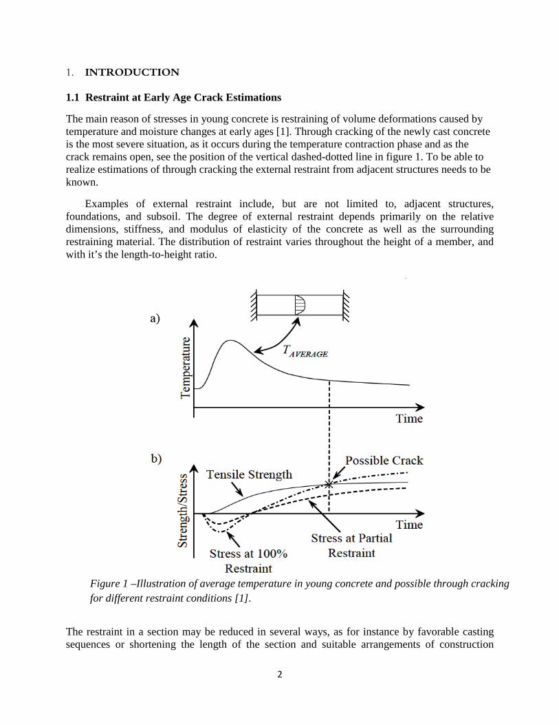
The main reason of stresses in young concrete is restraining of volume deformations caused by temperature and moisture changes at early ages [1]. Through cracking of the newly cast concrete is the most severe situation, as it occurs during the temperature contraction phase and as the crack remains open, see the position of the vertical dashed-dotted line in figure 1. To be able to realize estimations of through cracking the external restraint from adjacent structures needs to be known.

Examples of external restraint include, but are not limited to, adjacent structures, foundations, and subsoil. The degree of external restraint depends primarily on the relative dimensions, stiffness, and modulus of elasticity of the concrete as well as the surrounding restraining material. The distribution of restraint varies throughout the height of a member, and with it’s the length-to-height ratio.

The restraint in a section may be reduced in several ways, as for instance by favorable casting sequences or shortening the length of the section and suitable arrangements of construction

Figure 1 –Illustration of average temperature in young concrete and possible through cracking for different restraint conditions [1].

3

joints. It is also possible to mitigate early age through cracking by the choice of a concrete mix with low temperature rise due to hydration or lower the casting temperature [2]. Most common measures on site is to cool the newly cast concrete or to heat the adjacent structure, [1] and [2].

It is very important when analyzing the thermal stresses in the concrete at the early ages the amount of the restraint in the structure, the temperature generated at the casting and temperature difference between the concrete and the adjoining buildings; which are heavily influenced by the dimensions and geometry of the structures.

2. AIMS AND PURPOSES The aim and purposes of this report are to

• Analyze the use of artificial neural network calculating restraint situation for a typical case wall on the slab.

• Develop a simplified method for practical application using LRM for a typical case wall on slab

• To clarify the influences of geometrical dimensions on restraint in the wall. • To explain the importance ratio of study the geometrical properties of the walls on slabs

on the restraint.

3. ESTIMATION OF RESTRAINT IN EARLY AGE CONCRETE

In the literature there are many methods adopted to estimate and calculate the value of restraint in young concrete, see for example [3], [4], [5], [6] and [7]. Some of these methods need the use of a complex software, which usually is expensive and need experienced people. In this study, an artificial neural network (ANN) is presented to calculate the amount of restraint in the wall for typical structure wall-on-slab. The analyzes are based on results from 2920 elastic finite element calculations of the restraint in the wall founded on a slab [1], where the geometrical dimensions of the wall and the slab are varied systematically within reasonable values. The resulting restraints are fed and verified by an ANN, and the outcome from ANN are transformed to an Excel spread sheet to make the estimation of restraints quick and easy to apply for any engineer. This saves both time and money at estimation of the restraint curve for walls founded on a slab 3.1 Geometric effects on restraint early age concrete

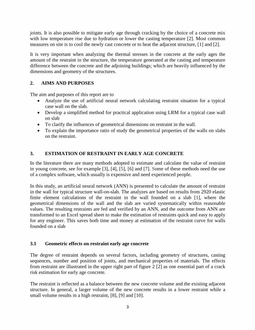
The degree of restraint depends on several factors, including geometry of structures, casting sequences, number and position of joints, and mechanical properties of materials. The effects from restraint are illustrated in the upper right part of figure 2 [2] as one essential part of a crack risk estimation for early age concrete. The restraint is reflected as a balance between the new concrete volume and the existing adjacent structure. In general, a larger volume of the new concrete results in a lower restraint while a small volume results in a high restraint, [8], [9] and [10].

4

In [9], and [10], it was shown in some ring tests that the degree of restraint depends only on the geometry and the material properties namely the elastic modulus and the Poisson’s ratio of the concrete and the steel. The degree of restraint increases with increasing the thickness and elastic modulus of the restraining steel rings and decreases with increasing the thickness of the concrete ring. The next chapter includes calculation of restraint in walls using the method of an artificial neural network based on geometric dimensions of the typical structure wall-on-slab.

Figure 2 - factors influencing temperatures –induced stresses and cracking in early age concrete [2].

5

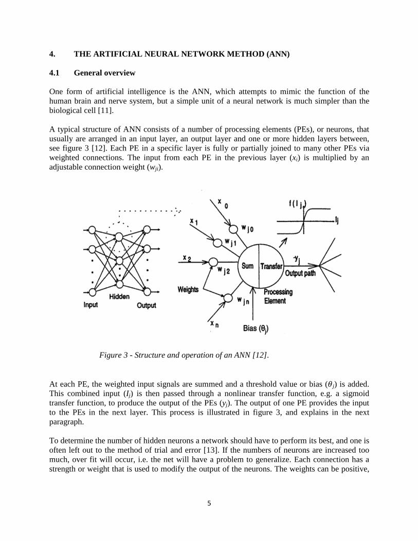
4. THE ARTIFICIAL NEURAL NETWORK METHOD (ANN) 4.1 General overview One form of artificial intelligence is the ANN, which attempts to mimic the function of the human brain and nerve system, but a simple unit of a neural network is much simpler than the biological cell [11]. A typical structure of ANN consists of a number of processing elements (PEs), or neurons, that usually are arranged in an input layer, an output layer and one or more hidden layers between, see figure 3 [12]. Each PE in a specific layer is fully or partially joined to many other PEs via weighted connections. The input from each PE in the previous layer (xi) is multiplied by an adjustable connection weight (wji). At each PE, the weighted input signals are summed and a threshold value or bias (𝜃j) is added. This combined input (Ij) is then passed through a nonlinear transfer function, e.g. a sigmoid transfer function, to produce the output of the PEs (yj). The output of one PE provides the input to the PEs in the next layer. This process is illustrated in figure 3, and explains in the next paragraph. To determine the number of hidden neurons a network should have to perform its best, and one is often left out to the method of trial and error [13]. If the numbers of neurons are increased too much, over fit will occur, i.e. the net will have a problem to generalize. Each connection has a strength or weight that is used to modify the output of the neurons. The weights can be positive,

Figure 3 - Structure and operation of an ANN [12].

6

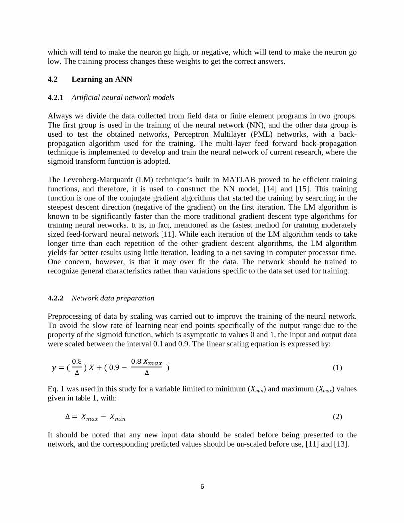
which will tend to make the neuron go high, or negative, which will tend to make the neuron go low. The training process changes these weights to get the correct answers. 4.2 Learning an ANN 4.2.1 Artificial neural network models Always we divide the data collected from field data or finite element programs in two groups. The first group is used in the training of the neural network (NN), and the other data group is used to test the obtained networks, Perceptron Multilayer (PML) networks, with a back-propagation algorithm used for the training. The multi-layer feed forward back-propagation technique is implemented to develop and train the neural network of current research, where the sigmoid transform function is adopted. The Levenberg-Marquardt (LM) technique’s built in MATLAB proved to be efficient training functions, and therefore, it is used to construct the NN model, [14] and [15]. This training function is one of the conjugate gradient algorithms that started the training by searching in the steepest descent direction (negative of the gradient) on the first iteration. The LM algorithm is known to be significantly faster than the more traditional gradient descent type algorithms for training neural networks. It is, in fact, mentioned as the fastest method for training moderately sized feed-forward neural network [11]. While each iteration of the LM algorithm tends to take longer time than each repetition of the other gradient descent algorithms, the LM algorithm yields far better results using little iteration, leading to a net saving in computer processor time. One concern, however, is that it may over fit the data. The network should be trained to recognize general characteristics rather than variations specific to the data set used for training. 4.2.2 Network data preparation Preprocessing of data by scaling was carried out to improve the training of the neural network. To avoid the slow rate of learning near end points specifically of the output range due to the property of the sigmoid function, which is asymptotic to values 0 and 1, the input and output data were scaled between the interval 0.1 and 0.9. The linear scaling equation is expressed by:

𝑦 = ( 0.8∆

) 𝑋 + ( 0.9 − 0.8 𝑋𝑚𝑎𝑥

∆ ) (1)

Eq. 1 was used in this study for a variable limited to minimum (Xmin) and maximum (Xmax) values given in table 1, with: ∆ = 𝑋𝑚𝑎𝑥 − 𝑋𝑚𝑖𝑛 (2) It should be noted that any new input data should be scaled before being presented to the network, and the corresponding predicted values should be un-scaled before use, [11] and [13].

7

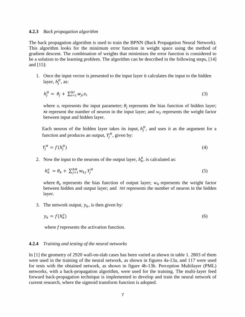
4.2.3 Back propagation algorithm The back propagation algorithm is used to train the BPNN (Back Propagation Neural Network). This algorithm looks for the minimum error function in weight space using the method of gradient descent. The combination of weights that minimizes the error function is considered to be a solution to the learning problem. The algorithm can be described in the following steps, [14] and [15]:

1. Once the input vector is presented to the input layer it calculates the input to the hidden layer, ℎ𝑗𝐻, as:

ℎ𝑗𝐻 = 𝜃𝑗 + ∑ 𝑤𝑗𝑖𝑥𝑖𝑁𝐼𝑖=1 (3)

where xi represents the input parameter; 𝜃𝑗 represents the bias function of hidden layer; NI represent the number of neuron in the input layer; and wji represents the weight factor between input and hidden layer. Each neuron of the hidden layer takes its input, ℎ𝑗𝐻, and uses it as the argument for a function and produces an output, 𝑌𝑗𝐻, given by: 𝑌𝑗𝐻 = 𝑓(ℎ𝑗𝐻) (4)

2. Now the input to the neurons of the output layer, ℎ𝑘0, is calculated as:

ℎ𝑘𝑜 = 𝜃𝑘 + ∑ 𝑤𝑘𝑗𝑁𝐻𝑗=1 𝑌𝑗𝐻 (5)

where 𝜃𝑘 represents the bias function of output layer; wkj represents the weight factor between hidden and output layer; and NH represents the number of neuron in the hidden layer.

3. The network output, 𝑦𝑘, is then given by:

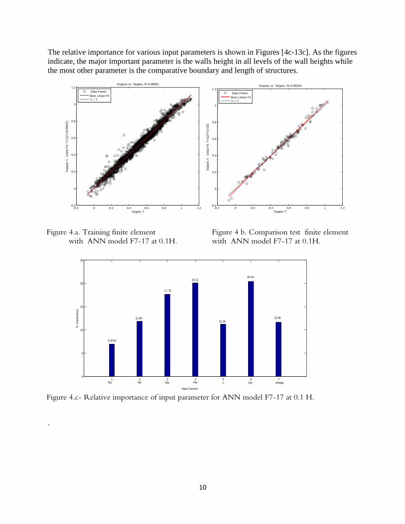
𝑦𝑘 = 𝑓(ℎ𝑘𝑜) (6) where f represents the activation function. 4.2.4 Training and testing of the neural networks In [1] the geometry of 2920 wall-on-slab cases has been varied as shown in table 1. 2803 of them were used in the training of the neural network, as shown in figures 4a-13a, and 117 were used for tests with the obtained network, as shown in figure 4b-13b. Perception Multilayer (PML) networks, with a back-propagation algorithm, were used for the training. The multi-layer feed forward back-propagation technique is implemented to develop and train the neural network of current research, where the sigmoid transform function is adopted.

8

As can be seen in the figures the coefficient of correlation, R, is closed to 1 at training and verification, which indicates that the resulting model is very good. In [1] the geometry of 2920 walls-on-slab cases has been varied as shown in table1. 2803 of them were used in the training of the neural networks, as shown in figure 4a-13a; 117 were used for tests with the obtained networks, as shown in figure 4b-13b. Perception Multilayer (PML) networks, with a back-propagation algorithm, were used for the training. The multi-layer feed forward back-propagation technique is implemented to develop and train the neural network of current research where the sigmoid transform function adopted. Table 1-List of parameters and their values used in the finite element method calculations of the elastic restraint variations in the walls of wall-on-slab structures.[1] Parameter Sample Maximum Minimum Unit Slab width Ba 8 2 m Wall width Bc 1.4 0.3 m Slab thickness Ha 1.8 0.4 m Wall height Hc 8 0.5 m Length of the structure

L 18 3 m

External rotational restraint

γ𝑟𝑟 1 0 -

Relative location* of the wall on slab

ω 1 0 -

*) ω = 0 means a wall placed in the middle of the slab; ω = 1 means a wall placed along the edge of the slab.

γ𝑟𝑟

9

5. STUDY OF IMPORTANCE GEOMETRY FACTORS MODEL

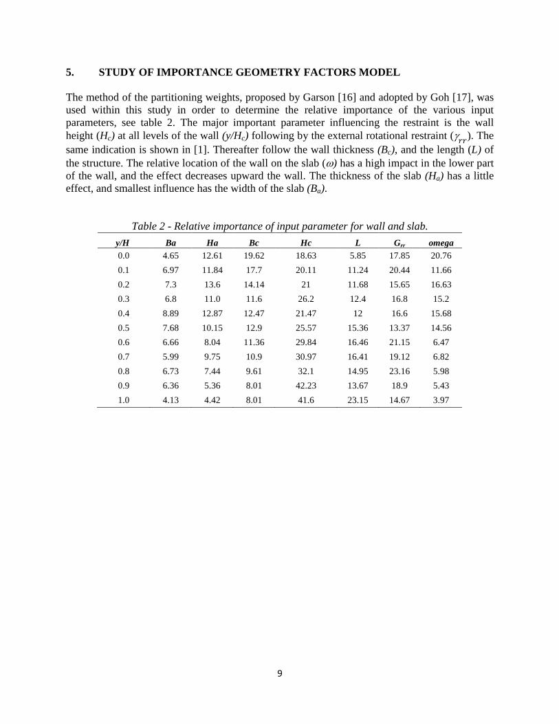
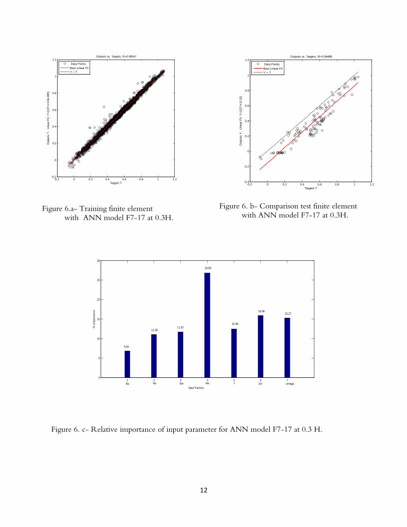
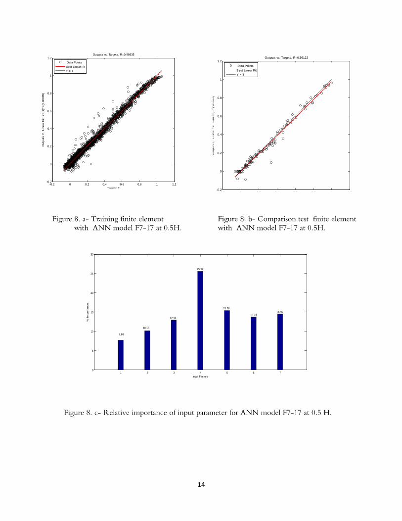
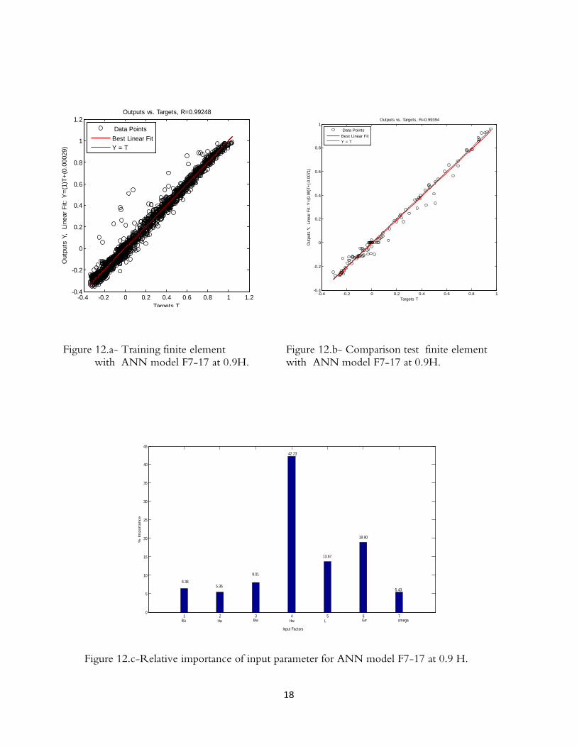
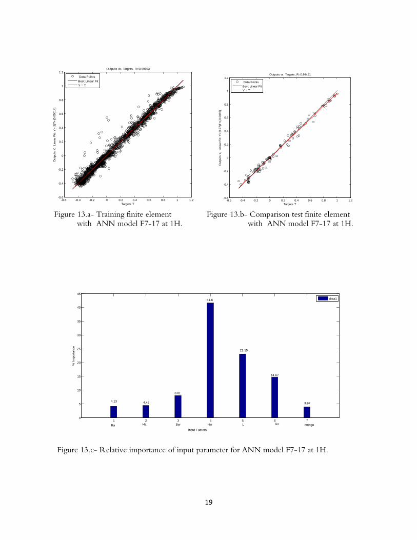
The method of the partitioning weights, proposed by Garson [16] and adopted by Goh [17], was used within this study in order to determine the relative importance of the various input parameters, see table 2. The major important parameter influencing the restraint is the wall height (Hc) at all levels of the wall (y/Hc) following by the external rotational restraint (γ𝑟𝑟). The same indication is shown in [1]. Thereafter follow the wall thickness (Bc), and the length (L) of the structure. The relative location of the wall on the slab (ω) has a high impact in the lower part of the wall, and the effect decreases upward the wall. The thickness of the slab (Ha) has a little effect, and smallest influence has the width of the slab (Ba).

Table 2 - Relative importance of input parameter for wall and slab. y/H Ba Ha Bc Hc L Grr omega 0.0 4.65 12.61 19.62 18.63 5.85 17.85 20.76 0.1 6.97 11.84 17.7 20.11 11.24 20.44 11.66 0.2 7.3 13.6 14.14 21 11.68 15.65 16.63 0.3 6.8 11.0 11.6 26.2 12.4 16.8 15.2 0.4 8.89 12.87 12.47 21.47 12 16.6 15.68 0.5 7.68 10.15 12.9 25.57 15.36 13.37 14.56 0.6 6.66 8.04 11.36 29.84 16.46 21.15 6.47 0.7 5.99 9.75 10.9 30.97 16.41 19.12 6.82 0.8 6.73 7.44 9.61 32.1 14.95 23.16 5.98 0.9 6.36 5.36 8.01 42.23 13.67 18.9 5.43 1.0 4.13 4.42 8.01 41.6 23.15 14.67 3.97

10

The relative importance for various input parameters is shown in Figures [4c-13c]. As the figures indicate, the major important parameter is the walls height in all levels of the wall heights while the most other parameter is the comparative boundary and length of structures.

`

-0.2 0 0.2 0.4 0.6 0.8 1 1.2-0.2

0

0.2

0.4

0.6

0.8

1

1.2

Targets T

Out

puts

Y,

Line

ar F

it: Y

=(1)

T+(0

.000

47)

Outputs vs. Targets, R=0.98902

Data PointsBest Linear FitY = T

-0.2 0 0.2 0.4 0.6 0.8 1 1.2-0.2

0

0.2

0.4

0.6

0.8

1

1.2

Targets TO

utpu

ts Y

, Li

near

Fit:

Y=(

1)T+

(-0.0

2)



1 2 3 4 5 6 70

5

10

15

20

25

% I

mpo

rtan

ce

Input Factors

6.9744

11.84

17.70

20.11

11.24

20.44

11.66

Ba Ha Bw Hw L Grr omega

Figure 4 b. Comparison test finite element with ANN model F7-17 at 0.1H.

Figure 4.a. Training finite element with ANN model F7-17 at 0.1H.

Figure 4.c- Relative importance of input parameter for ANN model F7-17 at 0.1 H.

11

-0.2 0 0.2 0.4 0.6 0.8 1 1.2-0.2

0

0.2

0.4

0.6

0.8

1

1.2

Targets T

Out

puts

Y,

Line

ar F

it: Y

=(1)

T+(-0

.000

15)



-0.2 0 0.2 0.4 0.6 0.8 1 1.2-0.4

-0.2

0

0.2

0.4

0.6

0.8

1

1.2

Targets T

Out

puts

Y,

Line

ar F

it: Y

=(1)

T+(-0

.12)



1 2 3 4 5 6 70

5

10

15

20

25

% I

mpo

rtan

ce

Input Factors

7.30

14.14

21.00

11.68

15.6516.63

13.61


Figure 5.a- Training finite element with ANN model F7-17 at 0.2H.

Figure 5.b- Comparison test finite element with ANN model F7-17 at 0.2H.

Figure 5. c. Relative importance of input parameter for ANN model F7-17 at 0.2H.

12

-0.2 0 0.2 0.4 0.6 0.8 1 1.2-0.2

0

0.2

0.4

0.6

0.8

1

1.2

Targets T

Out

puts

Y,

Line

ar F

it: Y

=(1)

T+(-3

.8e-

005)



-0.2 0 0.2 0.4 0.6 0.8 1 1.2-0.4

-0.2

0

0.2

0.4

0.6

0.8

1

1.2

Targets T

Out

puts

Y,

Line

ar F

it: Y

=(1)

T+(-0

.15)



1 2 3 4 5 6 70

5

10

15

20

25

30

% I

mpo

rtan

ce

Input Factors

6.81

11.0511.67

26.80

12.46

16.8615.27



Figure 6. b- Comparison test finite element with ANN model F7-17 at 0.3H.

Figure 6. c- Relative importance of input parameter for ANN model F7-17 at 0.3 H.

13

1 2 3 4 5 6 70

5

10

15

20

25

% I

mpo

rtan

ce

Input Factors

12.87

8.89

12.47

21.47

12.00

16.6015.68

HwBa Ha Bw L Grr omega

-0.2 0 0.2 0.4 0.6 0.8 1 1.2-0.2

0

0.2

0.4

0.6

0.8

1

1.2

Targets T

Out

puts

Y,

Line

ar F

it: Y

=(1)

T+(0

.000

39)



-0.2 0 0.2 0.4 0.6 0.8 1 1.2-0.2

0

0.2

0.4

0.6

0.8

1

1.2

Targets T

p

(

)(

)



Figure 7. a- Training finite element with ANN model F7-17 at 0.4H.



14

1 2 3 4 5 6 70

5

10

15

20

25

30

% I

mpo

rtan

ce

Input Factors

7.68

10.15

12.90

25.57

15.36

13.7314.56

-0.2 0 0.2 0.4 0.6 0.8 1 1.2-0.2

0

0.2

0.4

0.6

0.8

1

1.2

Targets T

Out

puts

Y,

Line

ar F

it: Y

=(1)

T+(0

.000

85)



0 2 0 0 2 0 4 0 6 0 8 1 1 2-0.2

0

0.2

0.4

0.6

0.8

1

1.2

Out

puts

Y,

Line

ar F

it: Y

=(0.

98)T

+(-0

.001

8)



Figure 8. a- Training finite element with ANN model F7-17 at 0.5H.



15

1 2 3 4 5 6 70

5

10

15

20

25

30

% I

mpo

rtan

ce

Input Factors

8.04

6.66

11.35

29.84

16.46

21.15

6.47

Ba BwHa Hw Grr omegaL

-0.2 0 0.2 0.4 0.6 0.8 1 1.2-0.2

0

0.2

0.4

0.6

0.8

1

1.2

Targets T

Out

puts

Y,

Line

ar F

it: Y

=(1)

T+(0

.000

76)



-0.2 0 0.2 0.4 0.6 0.8 1 1.2-0.2

0

0.2

0.4

0.6

0.8

1

1.2

Targets T

Out

puts

Y,

Line

ar F

it: Y

=(0.

96)T

+(0.

0015

)






16

1 2 3 4 5 6 70

5

10

15

20

25

30

35

% I

mpo

rtan

ce

Input Factors

30.97

10.909.75

5.99

16.41

19.12

6..82


-0.2 0 0.2 0.4 0.6 0.8 1 1.2-0.2

0

0.2

0.4

0.6

0.8

1

1.2

Targets T

Out

puts

Y,

Line

ar F

it: Y

=(0.

99)T

+(0.

0007

7)



-0.2 0 0.2 0.4 0.6 0.8 1 1.2-0.2

0

0.2

0.4

0.6

0.8

1

1.2

Targets T

Out

puts

Y,

Line

ar F

it: Y

=(0.

96)T

+(-0

.011

)






17

1 2 3 4 5 6 70

5

10

15

20

25

30

35

% I

mpo

rtan

ce

7.4484

9.6148

32.1034

14.9535

23.1604

5.98456.73

Ba HwBwHa L Grr omega

-0.4 -0.2 0 0.2 0.4 0.6 0.8 1 1.2-0.4

-0.2

0

0.2

0.4

0.6

0.8

1

1.2

Targets T

Out

puts

Y,

Line

ar F

it: Y

=(1)

T+(0

.000

7)



-0.4 -0.2 0 0.2 0.4 0.6 0.8 1-0.4

-0.2

0

0.2

0.4

0.6

0.8

1

T t TO

utpu

ts Y

, Li

near

Fit:

Y=(

1)T+

(-0.0

019)






18

1 2 3 4 5 6 70

5

10

15

20

25

30

35

40

45

% I

mpo

rtan

ce

Input Factors

6.365.36

8.01

42.23

13.67

18.90

5.43


-0.4 -0.2 0 0.2 0.4 0.6 0.8 1 1.2-0.4

-0.2

0

0.2

0.4

0.6

0.8

1

1.2

Targets T

Out

puts

Y,

Line

ar F

it: Y

=(1)

T+(0

.000

29)



-0.4 -0.2 0 0.2 0.4 0.6 0.8 1-0.4

-0.2

0

0.2

0.4

0.6

0.8

1

Targets T

Out

puts

Y,

Line

ar F

it: Y

=(0.

99)T

+(-0

.007

1)





Figure 12.c-Relative importance of input parameter for ANN model F7-17 at 0.9 H.

19

1 2 3 4 5 6 70

5

10

15

20

25

30

35

40

45

% Im

porta

nce

Input Factors

data1

4.13 4.42

8.01

41.6

23.15

14.67

3.97

Ba Bw HwHa L Grr omega

-0.6 -0.4 -0.2 0 0.2 0.4 0.6 0.8 1 1.2-0.6

-0.4

-0.2

0

0.2

0.4

0.6

0.8

1

1.2

Targets T

Out

puts

Y,

Line

ar F

it: Y

=(1)

T+(0

.000

14)



-0.6 -0.4 -0.2 0 0.2 0.4 0.6 0.8 1 1.2-0.6

-0.4

-0.2

0

0.2

0.4

0.6

0.8

1

1.2

Targets T

Out

puts

Y,

Line

ar F

it: Y

=(0.

97)T

+(-0

.003

5)



Figure 13.a- Training finite element with ANN model F7-17 at 1H.

Figure 13.b- Comparison test finite element with ANN model F7-17 at 1H.

Figure 13.c- Relative importance of input parameter for ANN model F7-17 at 1H.

20

2 4 6 8 10 12 14 16 180.1

0.2

0.3

0.4

0.5

0.6

0.7

0.8

0.9

rest

rain

t ra

tio

length of wall

Hc =0.5 Hc = 1Hc = 2Hc = 4 Hc = 8

Ba = 2Ha = 1Bc = 0.3Grr = 0omega = 0

2 4 6 8 10 12 14 16 180.1

0.2

0.3

0.4

0.5

0.6

0.7

0.8

0.9

rest

rain

t ra

tio

length of wall

Hc = 0.5Hc = 1Hc = 2Hc = 4Hc = 8

Ba = 2Ha = 1Bc = 0.3Grr = 0omega = 0

2 4 6 8 10 12 14 16 18-0.1

0

0.1

0.2

0.3

0.4

0.5

0.6

0.7

rest

rain

t ra

tio

length of wall

Hc = 0.5Hc = 1Hc = 2Hc = 4Hc = 8

Ba = 2Ha = 1Bc = 0.3Grr = 0omega = 0

2 4 6 8 10 12 14 16 180

0.1

0.2

0.3

0.4

0.5

0.6

0.7

rest

rain

t ra

tio

length of wall

Hc = 0.5Hc = 1Hc = 2Hc = 4Hc = 8

Ba = 2Ha = 1Bc = 0.3Grr = 0omega = 0

2 4 6 8 10 12 14 16 18-0.1

0

0.1

0.2

0.3

0.4

0.5

0.6

0.7

rest

rain

t ra

tio

length of wall

Hc = 0.5Hc = 1Hc = 2Hc = 4Hc = 8

Ba = 2Ha = 1Bc = 0.3Grr = 0omega = 0

2 4 6 8 10 12 14 16 18-0.2

-0.1

0

0.1

0.2

0.3

0.4

0.5

0.6

rest

rain

t ra

tio

length of wall

Hc = 0.5Hc = 1Hc = 2Hc = 4Hc = 8

Ba = 2Ha = 1Bc = 0.3Grr = 0omega = 0

2 4 6 8 10 12 14 16 18-0.4

-0.3

-0.2

-0.1

0

0.1

0.2

0.3

0.4

0.5

0.6

rest

rain

t ra

tio

length of wall

Hc = 0.5Hc = 1Hc = 2Hc = 4Hc = 8

Ba = 2Ha = 1Bc = 0.3Grr = 0omega =0

2 4 6 8 10 12 14 16 180.1

0.2

0.3

0.4

0.5

0.6

0.7

0.8

0.9

rest

rain

t ra

tio

length of wall

Hc = 0.5Hc = 1Hc = 2Hc = 4Hc = 8

Ba = 2Ha = 1Bc = 0.3grr =0omega = 0

6. STUDY OF PARAMETERS INFLUENCING THE RESTRAINT 6.1 Effect of wall height (Hc) The wall height is the most important factor affecting the degree of restraint in the case wall-on-slab, as shown in table 2. Generally, the degree of restraint decreases with an increase in wall height, which is compatible with the results shown in [1], [18], [19] and [20]. On the other hand, the restraint became bigger with increased wall length, as shown in figure 14, up to about 10m. Thereafter the restraint is no longer increasing with increased wall length

Figure 14- Variation of the Restraint with Length and Wall Height as predicted by ANN at Heights 0.1 H, 0.2H, 0.3H, 0.4 h, 0.5H, 0.6H, 0.8H, 1.0H

0.1H 0.2H

0.3H 0.4H

0.5H 0.6H

0.8H 1.0H

21

2 4 6 8 10 12 14 16 180.5

0.55

0.6

0.65

0.7

0.75

rest

rain

t ra

tio

length of wall

Ba = 2Ba = 3Ba = 4Ba =6 Ba = 8

Ha = 1Bc = 0.3Hc = 2Grr= 0omega = 0

2 4 6 8 10 12 14 16 180.52

0.54

0.56

0.58

0.6

0.62

0.64

0.66

0.68

0.7

0.72

rest

rain

t ra

tio

length of wall

Ba = 2Ba = 3Ba = 4Ba = 6Ba = 8

Ha = 1Bc = 0.3Hc = 2Grr = 0omega = 0

2 4 6 8 10 12 14 16 18

0.2

0.25

0.3

0.35

0.4

0.45

0.5

rest

rain

t ra

tio

length of wall

Ba = 2Ba = 3Ba = 4Ba = 6Ba = 8

Ha = 1Bc = 0.3Hc = 2Grr = 0omega = 0

2 4 6 8 10 12 14 16 180.05

0.1

0.15

0.2

0.25

0.3

0.35

0.4

0.45

rest

rain

t ra

tio

length of wall

Ba = 2Ba = 3Ba = 4Ba = 6Ba = 8

Ha = 1Bc = 0.3Hc = 2Grr = 0omega = 0

2 4 6 8 10 12 14 16 180

0.05

0.1

0.15

0.2

0.25

0.3

0.35

rest

rain

t ra

tio

length of wall

Ba = 2Ba = 3Ba = 4Ba = 6Ba = 8

Ha =1Bc = 0.3H = 2Grr = 0omega = 0

2 4 6 8 10 12 14 16 18-0.1

-0.05

0

0.05

0.1

0.15

rest

rain

t ra

tio

length of wall

Ba = 2Ba = 3 Ba = 4Ba = 6Ba = 8

Ha = 1Bc = 0.3Hc = 2Grr = 0omega = 0

2 4 6 8 10 12 14 16 18-0.3

-0.25

-0.2

-0.15

-0.1

-0.05

0

0.05

0.1

rest

rain

t ra

tio

length of wall

Ba = 2Ba = 3Ba = 4Ba = 6Ba = 8

Ha = 1Bc = 0.3Hc = 2Grr = 0omega = 0

2 4 6 8 10 12 14 16 180.54

0.56

0.58

0.6

0.62

0.64

0.66

0.68

0.7

0.72

rest

rain

t ra

tio

length of wall

Ba = 2Ba = 3Ba = 4Ba = 6Ba = 8

Ha = 1Bc = 0.3Hc = 2Grr = 0omega = 0

6.2 Effect of Slab Width

Generally, the value of restraint increases with the increase of the slab width for all levels of the wall height. A smaller increase in the value of restraint is observed with the increase in structural length beyond 10m (for L/Hc > 5), see figure 15. The same indication is found in [3], [20], [21], and [22]

Figure 15- Variation of the Restraint with Length and Slab Width as predicted by ANN at Heights 0.1 H, 0.2H, 0.3H, 0.4 h, 0.5H, 0.6H, 0.8H, 1.0H

0.1H 0.2H

0.3H 0.4H

0.5H 0.6H

0.8 H 1.0 H

22

2 4 6 8 10 12 14 16 180.52

0.54

0.56

0.58

0.6

0.62

0.64

0.66

rest

rain

t ra

tio

length of wall

Ha = 0.4Ha = 0.7Ha = 1Ha = 1.2Ha = 1.2

Ba = 2Bc = 0.3Hc = 2Grr = 0omega = 0

2 4 6 8 10 12 14 16 180.1

0.15

0.2

0.25

0.3

0.35

rest

rain

t ra

tio

length of wall

Ha = 0.4Ha = 0.7Ha = 1Ha = 1.2Ha = 1.4

Ba = 2Bc = 0.3Hc = 2Grr = 0omega = 0

2 4 6 8 10 12 14 16 180.05

0.1

0.15

0.2

0.25

0.3

rest

rain

t ra

tio

length of wall

Ha = 0.4Ha = 0.7Ha = 1Ha = 1.2Ha = 1.4

Ba = 2Bc = 0.3Hc = 2Grr = 0omega = 0

2 4 6 8 10 12 14 16 18-0.05

0

0.05

0.1

0.15

0.2

rest

rain

t ra

tio

length of wall

Ha = 0.4Ha = 0.7Ha = 1Ha = 1.2Ha = 1.4

Ba = 2Bc = 0.3Hc = 2Grr = 0omega = 0

2 4 6 8 10 12 14 16 18-0.2

-0.15

-0.1

-0.05

0

0.05

rest

rain

t ra

tio

length of wall

Ha = 0.4Ha = 0.7Ha = 1Ha = 1.2Ha = 1.4

Ba = 2Bc = 0.3Hc = 2Grr = 0omega = 0

2 4 6 8 10 12 14 16 18-0.45

-0.4

-0.35

-0.3

-0.25

-0.2

-0.15

-0.1

-0.05

rest

rain

t ra

tio

length of wall

Ha =0.4Ha = 0.7Ha = 1Ha =1.2Ha = 1.4

Ba = 2Bc = 0.3Hc = 2Grr = 0omega = 0

2 4 6 8 10 12 14 16 180.52

0.54

0.56

0.58

0.6

0.62

0.64

0.66

rest

rain

t ra

tio

length of wall

Ha = 0.4Ha = 0.7Ha =1Ha = 1.2Ha = 1.4

Ba = 2Bc = 0.3Hc = 2Grr = 0omega = 0

2 4 6 8 10 12 14 16 180.5

0.52

0.54

0.56

0.58

0.6

0.62

0.64

0.66

0.68

rest

rain

t ra

tio

length of wall

Ha = 0.4Ha = 0.7 Ha = 1Ha 1.2Ha = 1.4

Ba = 2Bc = 0.3Hc = 2Grr =0omega = 0

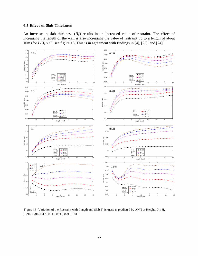
6.3 Effect of Slab Thickness

An increase in slab thickness (Ha) results in an increased value of restraint. The effect of increasing the length of the wall is also increasing the value of restraint up to a length of about 10m (for L/Hc ≤ 5), see figure 16. This is in agreement with findings in [4], [23], and [24].

Figure 16- Variation of the Restraint with Length and Slab Thickness as predicted by ANN at Heights 0.1 H, 0.2H, 0.3H, 0.4 h, 0.5H, 0.6H, 0.8H, 1.0H

1.0 H

0.1 H 0.2 H

0.3 H 0.4 H

0.5 H 0.6 H

0.8 H

23

2 4 6 8 10 12 14 16 180.45

0.5

0.55

0.6

0.65

0.7

rest

rain

t ra

tio

length of wall

Bc = 0.3Bc = 0.65Bc = 1Bc = 1.4Bc = 1.8

Ba = 2Ha = 1Hc = 2Grr = 0omega = 0

2 4 6 8 10 12 14 16 180.48

0.5

0.52

0.54

0.56

0.58

0.6

0.62

0.64

0.66

rest

rain

t ra

tio

length of wall

Bc = 0.3Bc = 0.65Bc = 1 Bc = 1.4Bc = 1.8

Ba = 2Ha = 1Hc = 2Grr= 0omega =0

2 4 6 8 10 12 14 16 180.1

0.15

0.2

0.25

0.3

0.35

rest

rain

t ra

tio

length of wall

Bc = 0.3Bc = 0.65Bc = 1Bc = 1.4Bc = 1.8


2 4 6 8 10 12 14 16 180.05

0.1

0.15

0.2

0.25

rest

rain

t ra

tio

length of wall

Bc = 0.3Bc = 0.65Bc = 1Bc = 1.4Bc = 1.8

Ba = 2Ha = 1Hc2Grr = 0omega = 0

2 4 6 8 10 12 14 16 18-0.02

0

0.02

0.04

0.06

0.08

0.1

0.12

0.14

0.16

rest

rain

t ra

tio

length of wall

Bc = 0.3Bc = 0.65Bc = 1Bc = 1.4Bc = 1.8


2 4 6 8 10 12 14 16 18-0.24

-0.22

-0.2

-0.18

-0.16

-0.14

-0.12

-0.1

-0.08

-0.06

rest

rain

t ra

tio

length of wall

Bc = 0.3Bc = 0.65Bc = 1Bc = 1.4Bc = 1.8


2 4 6 8 10 12 14 16 18-0.4

-0.35

-0.3

-0.25

-0.2

-0.15

rest

rain

t ra

tio

length of wall

Bc = 0.3 Bc = 0.65Bc = 1Bc = 1.4Bc = 1.8


6.4 Effect of Wall Thickness

Increase of the size of the new concrete means higher possibility of counteracting the external constraints (from old concrete, i.e the slab in this case), which is reflected in figure 17 as the restraint will decrease with increased wall thickness. Besides, up to a structural length of 10m (for L/Hc ≤ 5) the restraint increases with increased structure length, which is in agreement with results in [3], [24] and [25].

2 4 6 8 10 12 14 16 180.46

0.48

0.5

0.52

0.54

0.56

0.58

0.6

0.62

0.64

rest

rain

t ra

tio

length of wall

Bc = 0.3Bc = 0.65Bc = 1Bc = 1.4Bc = 1.8

Ba= 2Ha = 1Hc = 2Grr = 0omega = 0

Figure 17- Variation of the Restraint with Length and Wall Thickness as predicted by ANN at Heights 0.1 H, 0.2H, 0.3H, 0.4 h, 0.5H, 0.6H, 0.8H, 1.0H

0.1 H 0.2 H

0.3 H 0.4 H

0.5 H 0.6 H

0.8 H 1.0 H

24

2 4 6 8 10 12 14 16 180.5

0.55

0.6

0.65

0.7

0.75

rest

rain

t ra

tio

length of wall

grr = 0grr = 1

Ba= 2Ha = 1Bc = 0.3Hc = 2Omega = 0

2 4 6 8 10 12 14 16 180.5

0.55

0.6

0.65

0.7

0.75

0.8

0.85

0.9

rest

rain

t ra

tio

length of wall

grr = 0grr = 1

Ba = 2Ha = 1Bc = 0.3Hc = 2omega = 0

2 4 6 8 10 12 14 16 180.1

0.2

0.3

0.4

0.5

0.6

0.7

0.8

rest

rain

t ra

tio

length of wall

grr = 0grr = 1

Ba =2Ha = 1Bc = 0.3Hc = 2omega = 0

2 4 6 8 10 12 14 16 180

0.1

0.2

0.3

0.4

0.5

0.6

0.7

0.8

rest

rain

t ra

tio

length of wall

grr = 0grr = 1

Ba = 2Ha = 1Bc = 0.3Hc = 2omega = 0

2 4 6 8 10 12 14 16 180

0.1

0.2

0.3

0.4

0.5

0.6

0.7

0.8

rest

rain

t ra

tio

length of wall

grr = 0 grr = 1

Ba = 2Ha = 1Bc = 0.3Hc = 2omega = 0

2 4 6 8 10 12 14 16 18-0.1

0

0.1

0.2

0.3

0.4

0.5

0.6

0.7

0.8

rest

rain

t ra

tio

length of wall

grr=0grr = 1

Ba = 2Ha = 1Bc = 0.3Hc = 2omega = 0

2 4 6 8 10 12 14 16 18-0.4

-0.2

0

0.2

0.4

0.6

0.8

1

rest

rain

t ra

tio

l th f ll

grr = 0grr = 1

Ba = 2Ha = 1Bc = 0.3Hc = 2omega = 0

2 4 6 8 10 12 14 16 180.5

0.55

0.6

0.65

0.7

0.75

0.8

0.85

0.9

rest

rain

t ra

tio

length of wall

grr = 0grr = 1

Ba = 2Ha = 1Bc = 0.3Hc = 2omega = 0

6.5 Effect of rotational boundary restraint (Grr) As shown in table 2, the second parameter of influence on restraint is the external rotational restraint. The bending moment during a contraction in a wall rotates the ends of the structure upward and the center downward. If the material under the foundation is stiff, the resistance on the structure is high, which at total rotational stiff ground reflects by γrr equal to 1. If the material under the foundations is very soft, the value of γrr is zero. The results of the ANN with γrr =1 showed high restraint, which is in line with results in [22]. The restraint is about 40% lower when γrr is equal to zero. For both γrr = 1 and γrr = 0 the restraint increases with length of the structures up to about 10m (for L/Hc ≤ 5), see figure 18

Figure 18- Variation of the Restraint with Length and Rotational Boundary as predicted by ANN at Heights 0.1 H, 0.2H, 0.3H, 0.4 h, 0.5H, 0.6H, 0.8H, 1.0H

0.1 H 0.2 H

0.3 H 0.4 H

0.5 H 0.6 H

0.8 H 1.0 H

Grr=0 Grr=1

Grr=0 Grr=1

Grr=0 Grr=1

Grr=0 Grr=1

Grr=0 Grr=1

Grr=0 Grr=1

Grr=0 Grr=1

Grr=0 Grr=1

25

2 4 6 8 10 12 14 16 180.4

0.45

0.5

0.55

0.6

0.65

0.7

0.75

rest

rain

t ra

tio

length of wall

omega = 0omega = 0.25omega = 0.5omega = 0.75omega = 1

Ba = 2Ha = 1Bc = 0.3Hc = 2Grr =0

2 4 6 8 10 12 14 16 180.44

0.46

0.48

0.5

0.52

0.54

0.56

0.58

0.6

0.62

0.64

rest

rain

t ra

tio

length of wall

omega = 0omega = 0.25omega = 0.5omega = 1omega =1

Ba = 2Ha = 1Bc = 0.3Hc = 2L = 3Grr = 0

2 4 6 8 10 12 14 16 180.44

0.46

0.48

0.5

0.52

0.54

0.56

0.58

0.6

0.62

0.64

rest

rain

t ra

tio

length of wall


Ba = 2Ha = 1Bc = 0.3Hc = 2Grr = 0

2 4 6 8 10 12 14 16 18

0.16

0.18

0.2

0.22

0.24

0.26

0.28

0.3

0.32

0.34

rest

rain

t ra

tio

length of wall

omega = 0.0omega = 0.25omega = 0.5omega = 0.75omega = 1.0

Ba =2Ha =1Bc =0.3Hc = 2Grr = 0

2 4 6 8 10 12 14 16 180.08

0.1

0.12

0.14

0.16

0.18

0.2

0.22

0.24

0.26

rest

rain

t ra

tio

length of wall


Ba = 2Ha = 1Bc = 0.3Hc = 2Grr = 0

2 4 6 8 10 12 14 16 180.02

0.04

0.06

0.08

0.1

0.12

0.14

0.16

0.18

rest

rain

t ra

tio

length of wall


Ba = 2Ha = 1Bc = 0.3Hc = 2Grr = 0

2 4 6 8 10 12 14 16 18-0.13

-0.12

-0.11

-0.1

-0.09

-0.08

-0.07

-0.06

-0.05

-0.04

-0.03

rest

rain

t ra

tio

length of wall

omega = 0.0omega = 0.25omega = 0.5omega = 0.75omega = 1

Ba = 2Ha = 1Bc = 0.3Hc = 2Grr = 0

2 4 6 8 10 12 14 16 18-0.26

-0.25

-0.24

-0.23

-0.22

-0.21

-0.2

-0.19

-0.18

-0.17

-0.16

rest

rain

t ra

tio

length of wall


Ba = 8Ha = 1Bc = 0.3Hc = 2Grr = 0

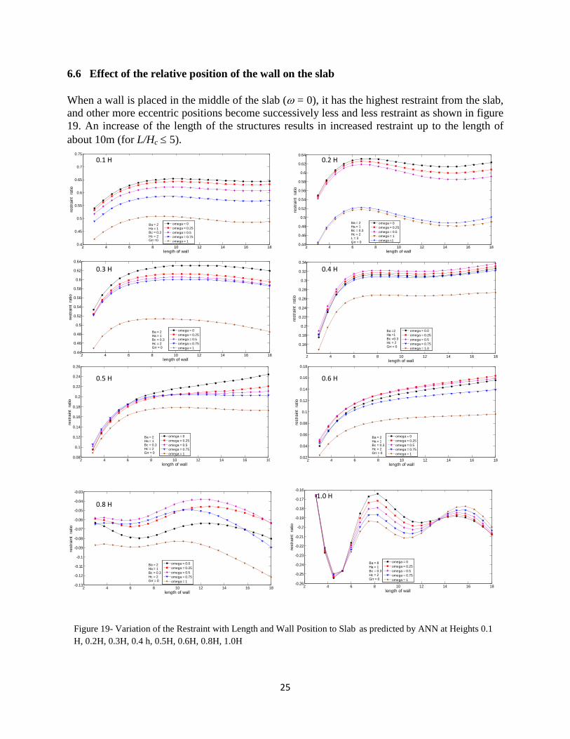
6.6 Effect of the relative position of the wall on the slab When a wall is placed in the middle of the slab (ω = 0), it has the highest restraint from the slab, and other more eccentric positions become successively less and less restraint as shown in figure 19. An increase of the length of the structures results in increased restraint up to the length of about 10m (for L/Hc ≤ 5).

Figure 19- Variation of the Restraint with Length and Wall Position to Slab as predicted by ANN at Heights 0.1 H, 0.2H, 0.3H, 0.4 h, 0.5H, 0.6H, 0.8H, 1.0H

0.1 H 0.2 H

0.3 H 0.4 H

1.0 H

0.5 H 0.6 H

0.8 H

26

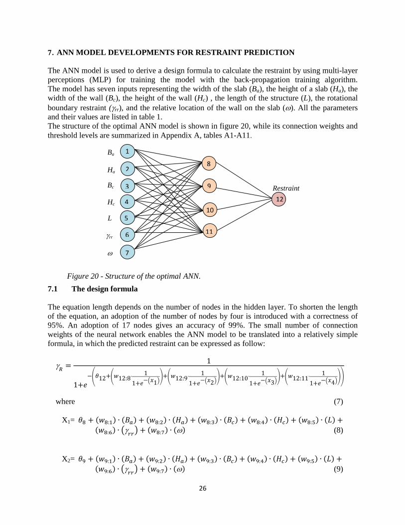
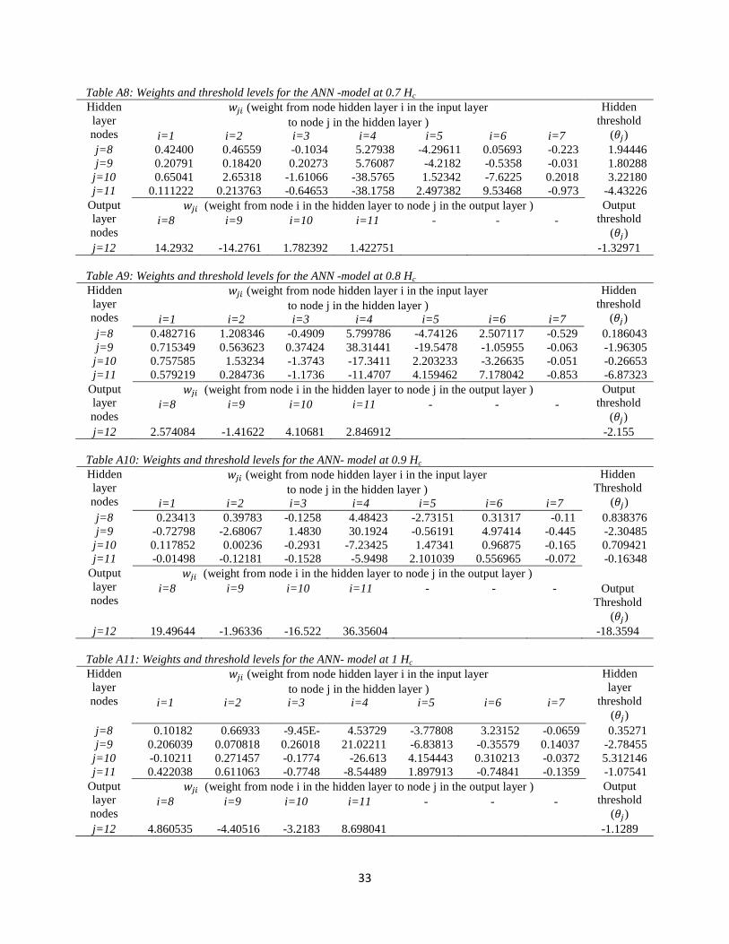
7. ANN MODEL DEVELOPMENTS FOR RESTRAINT PREDICTION The ANN model is used to derive a design formula to calculate the restraint by using multi-layer perceptions (MLP) for training the model with the back-propagation training algorithm. The model has seven inputs representing the width of the slab (Ba), the height of a slab (Ha), the width of the wall (Bc), the height of the wall (Hc) , the length of the structure (L), the rotational boundary restraint (γrr), and the relative location of the wall on the slab (ω). All the parameters and their values are listed in table 1. The structure of the optimal ANN model is shown in figure 20, while its connection weights and threshold levels are summarized in Appendix A, tables A1-A11. 7.1 The design formula The equation length depends on the number of nodes in the hidden layer. To shorten the length of the equation, an adoption of the number of nodes by four is introduced with a correctness of 95%. An adoption of 17 nodes gives an accuracy of 99%. The small number of connection weights of the neural network enables the ANN model to be translated into a relatively simple formula, in which the predicted restraint can be expressed as follow: γ𝑅 = 1

1+𝑒−�𝜃12+�𝑤12:8∙

11+𝑒−�𝑥1�

�+�𝑤12:9∙1

1+𝑒−�𝑥2��+�𝑤12:10∙

11+𝑒−�𝑥3�

�+�𝑤12:11∙1

1+𝑒−�𝑥4��

where (7)

X1= 𝜃8 + (𝑤8:1) ∙ (𝐵𝑎) + (𝑤8:2) ∙ (𝐻𝑎) + (𝑤8:3) ∙ (𝐵𝑐) + (𝑤8:4) ∙ (𝐻𝑐) + (𝑤8:5) ∙ (𝐿) + (𝑤8:6) ∙ �γ𝑟𝑟� + (𝑤8:7) ∙ (ω) (8)

X2= 𝜃9 + (𝑤9:1) ∙ (𝐵𝑎) + (𝑤9:2) ∙ (𝐻𝑎) + (𝑤9:3) ∙ (𝐵𝑐) + (𝑤9:4) ∙ (𝐻𝑐) + (𝑤9:5) ∙ (𝐿) + (𝑤9:6) ∙ �γ𝑟𝑟� + (𝑤9:7) ∙ (ω) (9)

Figure 20 - Structure of the optimal ANN.

Ba

Bc

Ha

Hc

L

γrr

ω

Restraint 12

1

2

3

4

5

6

7

8

9

10

11

27

00.10.20.30.40.50.60.70.80.9

1

0 0.1 0.2 0.3 0.4 0.5 0.6 0.7 0.8 0.9 1

FEExcel sheet

Restraint

y/H

X3= 𝜃10 + (𝑤10:1) ∙ (𝐵𝑎) + (𝑤10:2) ∙ (𝐻𝑎) + (𝑤10:3) ∙ (𝐵𝑐) + (𝑤10:4) ∙ (𝐻𝑐) + (𝑤10:5) ∙ (𝐿) + (𝑤10:6) ∙ �γ𝑟𝑟� + (𝑤10:7) ∙ (ω) (10) X4= 𝜃11 + (𝑤11:1) ∙ (𝐵𝑎) + (𝑤11:2) ∙ (𝐻𝑎) + (𝑤11:3) ∙ (𝐵𝑐) + (𝑤11:4) ∙ (𝐻𝑐) + (𝑤11:5) ∙ (𝐿) + (𝑤11:6) ∙ �γ𝑟𝑟� + (𝑤11:7) ∙ (ω) (11)

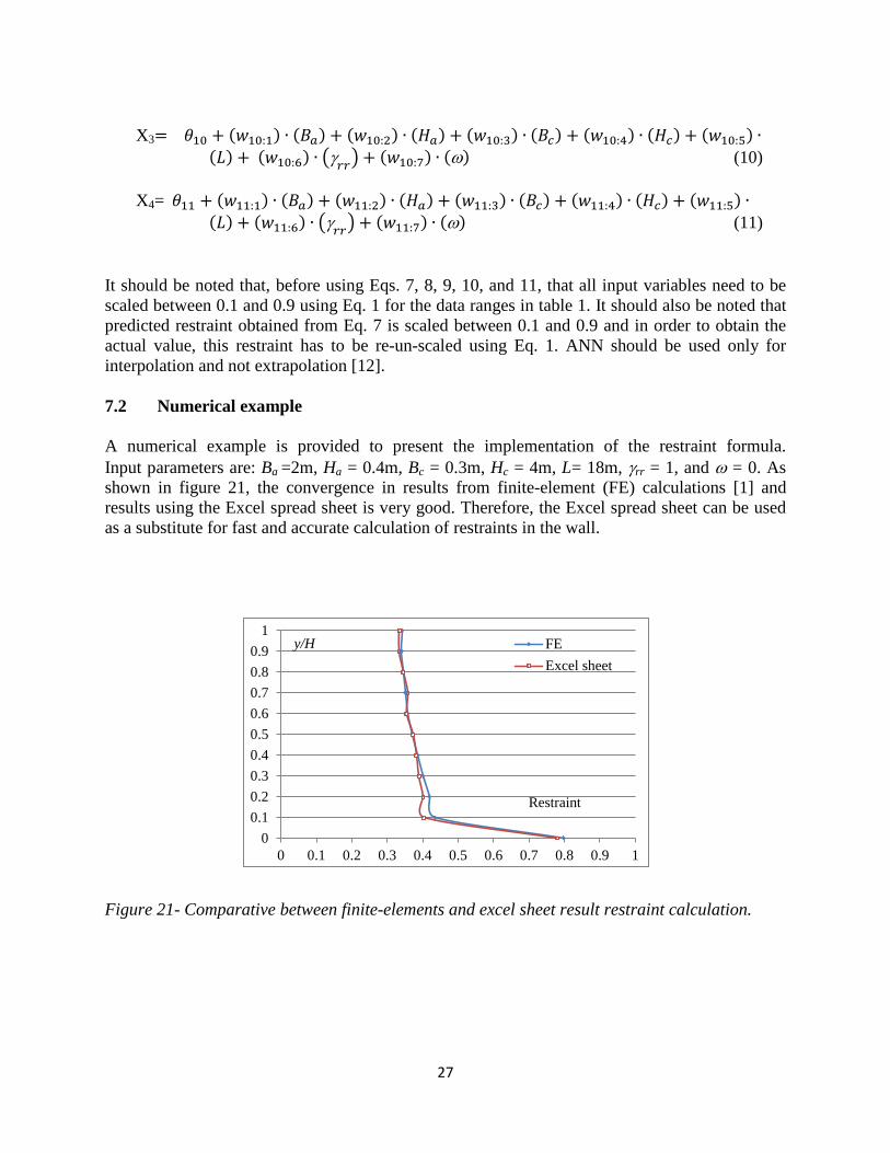
It should be noted that, before using Eqs. 7, 8, 9, 10, and 11, that all input variables need to be scaled between 0.1 and 0.9 using Eq. 1 for the data ranges in table 1. It should also be noted that predicted restraint obtained from Eq. 7 is scaled between 0.1 and 0.9 and in order to obtain the actual value, this restraint has to be re-un-scaled using Eq. 1. ANN should be used only for interpolation and not extrapolation [12]. 7.2 Numerical example A numerical example is provided to present the implementation of the restraint formula. Input parameters are: Ba =2m, Ha = 0.4m, Bc = 0.3m, Hc = 4m, L= 18m, γrr = 1, and ω = 0. As shown in figure 21, the convergence in results from finite-element (FE) calculations [1] and results using the Excel spread sheet is very good. Therefore, the Excel spread sheet can be used as a substitute for fast and accurate calculation of restraints in the wall. Figure 21- Comparative between finite-elements and excel sheet result restraint calculation.

28

8. CONCLUSIONS Existing research concerning restraint curves has been applied to the method of artificial neural networks to model restraint in the wall for the typical structure wall-on-slab. Seven input parameters have been used, and it has been proven that the neural network is capable of modeling the restraint with good accuracy. The usage of the neural network has been demonstrated to give a clear picture of the relative importance of the input parameters. The dimension of the wall (height and width) as well as the external rotational restraint turned out to give the highest importance on restraint in the wall. On the opposite, the width of the slab was found to be of least significance in this respect. Further, it is shown that the results from the neural network can be represented by a series of basic weight and response functions. Resulting functions can easily be implemented to simple computer tools. Thus, the results can easily be made available to any engineer without use of complicated software.

29

8. REFERENCES 1. Nilsson, M., “Restraint Factors and Partial Coefficients for Crack Risk Analyses of

Early Age Concrete Structures”, Lulea, Sweden, Division of Structural Engineering, Lulea University of Technology, Doctoral Thesis 2003:19, 170 pp.

2. Emborg, M., & Bernander, S., “Assessment of the Risk of Thermal Cracking in Hardening Concrete”, Journal of Structural Engineering (ASCE), Vol.120, No 10, October 1994, pp. 2893-2912.

3. ACI Committee 207, “Effect of Restraint, Volume Change, and Reinforcement on Cracking of Massive Concrete”, ACI Committee 207.ACI207.2R-1995. Reapproved 2002, 26 pp.

4. JSCE, “English Version of Standard Specification for Concrete Structures 2007”, Japan Society of Civil Engineer, JSCE, December 2010, 503 pp.

5. Cusson, D., & Hoogeveen, T., “An Experimental Approach for the Analysis of Early Age Behavior of High Performance Concrete Structures Under Restrained Shrinkage”, Cement and Concrete Research, 2007, 37: 2, pp. 200-209.

6. Bamforth, P. B., “Early-age Thermal Crack Control in Concrete”, CIRIA Report C660, Construction Industry Research and Information Association, London, 2007.

7. Olofsson, J., Bosnjak, D., Kanstad, T., “Crack Control of Hardening Concrete Structures Verification of Three Steps Engineering Methods”, 2000, 13th Nordic Seminar on Computational Mechanics, Oslo.

9. Weiss, W. J., Yang, W., Shah, S. P., “Influence of Specimen Size/Geometry on Shrinkage Cracking of Rings”, Journal of Engineering Mechanics, Vol. 126, No. 1, January, 2000, pp. 93-101.

9. Moon, J.H., Rajabipour, F., Pease, B., Weiss, J., “Quantifying the Influence of Specimen Geometry on the Results of the Restrained Ring Test”, Journal of ASTM International, Vol. 3, No. 8, 2006, pp. 1-14.

10. Hossain, A.B., & Weiss, J., “The Role of Specimen Geometry and Boundary Conditions on Stress Development and Cracking in the Restrained Ring Test”, Cement and Concrete Research, 36, 2006, pp. 189– 199.

11. Yousif, S. T., & Al-Jurmaa, M. A., “Modeling of Ultimate Load for R.C. Beams Strengthened with Carbon FRP using Artificial Neural Networks”, Al-Rafidain Engineering, Vol.18, No.6, December 2010, pp. 28-41.

12. Shahin, M.A., Jaksa, M.B, Maier, H.R., “Artificial Neural Network−Based Settlement Prediction Formula for Shallow Foundations on Granular Soils”, Australian Geomechanics September 2002, pp. 45-52.

13. Yousif, S. T., “Artificial Neural Network Modeling of Elasto-Plastic Plates”, Ph.D. thesis, College of Engineering, Mosul University, Iraq, 2007, 198 pp.

14. Hudson B., Hagan, M., Demuth, H., “Neural Network Toolbox for Use with MATLAB”, User’s Guide, the Math works, 2012.

15. Hagan, M.T., Demuth, H.B., Beale, M.H., “Neural Network Design”, Boston, MA: PWS Publishing, 1996.

16. Garson, G.D., “Interpreting Neural Network Connection Weights”, Artificial Intelligence, Vol. 6, 1991, pp. 47-51.

javascript:visitAuthor(%22D_Cusson%22)

javascript:visitAuthor(%22T_Hoogeveen%22)

30

17. Goh, A.T.C., “Back-Propagation Neural Networks for Modeling Complex Systems”, Artificial Intelligence in Engineering, Vol.9, No.3, 1995, pp. 143-151.

18. Emborg M., “Thermal Stresses in Concrete Structures at Early Ages”, Div. of Structural Engineering, Lulea University of Technology, Doctoral Thesis, 73D, 1989, 280 pp.

19. Kheder, G. F, Al-Rawi, R. S., Al-Dhahi, J. K., “A Study of the Behavior of Volume Change Cracking in Base Restrained Concrete Walls”, Materials and Structures, 27, 1994, pp. 383-392.

20. Kheder, G.F., “A New Look at the Control of Volume Change Cracking of Base Restrained Concrete Walls”, ACI Structural. Journal, 94 (3), 1997, pp. 262-271.

21. Nagy A. “Parameter Study of Thermal Cracking in HPC and NPC Structures”, Nordic Concrete Research, No.26, 2001/1.

22. Kwak, H.G., & Ha, S.J., “Non-Structural Cracking in RC Walls: Part II. Quantitative Prediction Model”, Cement and Concrete Research 36, 2006, pp. 761–775.

23. Lin, F., Song, X., Gu, X., Peng, B., Yang, L., “Cracking Analysis of Massive Concrete Walls with Cracking Control Techniques”, Construction and Building Materials, 31, 2012, pp. 12–21.

24. Kim S.C., “Effects of a Lift Height on the Thermal Cracking in Wall Structures”, KCI Concrete Journal (Vo1.12 No.1), 2000, pp. 47-56.

25. Larson M., “Evaluation of Restraint from Adjoining Structures”, IPACS-Rep, Lulea University of Technology, Lulea, Sweden, 1999.

31

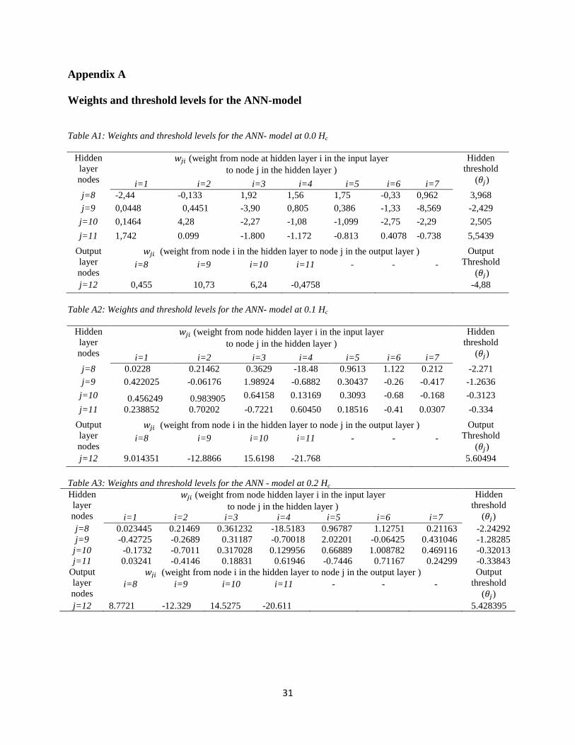
Appendix A Weights and threshold levels for the ANN-model Table A1: Weights and threshold levels for the ANN- model at 0.0 Hc

Hidden layer nodes

𝑤𝑗𝑖 (weight from node at hidden layer i in the input layer to node j in the hidden layer )

Hidden threshold

(𝜃𝑗) i=1 i=2 i=3 i=4 i=5 i=6 i=7 j=8 -2,44 -0,133 1,92 1,56 1,75 -0,33 0,962 3,968 j=9 0,0448 0,4451 -3,90 0,805 0,386 -1,33 -8,569 -2,429

j=10 0,1464 4,28 -2,27 -1,08 -1,099 -2,75 -2,29 2,505 j=11 1,742 0.099 -1.800 -1.172 -0.813 0.4078 -0.738 5,5439

Output layer nodes

𝑤𝑗𝑖 (weight from node i in the hidden layer to node j in the output layer ) Output Threshold

(𝜃𝑗) i=8 i=9 i=10 i=11 - - -

j=12 0,455 10,73 6,24 -0,4758 -4,88 Table A2: Weights and threshold levels for the ANN- model at 0.1 Hc

Hidden layer nodes

𝑤𝑗𝑖 (weight from node hidden layer i in the input layer to node j in the hidden layer )

Hidden threshold

(𝜃𝑗) i=1 i=2 i=3 i=4 i=5 i=6 i=7 j=8 0.0228 0.21462 0.3629 -18.48 0.9613 1.122 0.212 -2.271 j=9 0.422025 -0.06176 1.98924 -0.6882 0.30437 -0.26 -0.417 -1.2636

j=10 0.456249

0.983905

0.64158 0.13169 0.3093 -0.68 -0.168 -0.3123 j=11 0.238852 0.70202 -0.7221 0.60450 0.18516 -0.41 0.0307 -0.334

Output layer nodes

𝑤𝑗𝑖 (weight from node i in the hidden layer to node j in the output layer ) Output Threshold

(𝜃𝑗) i=8 i=9 i=10 i=11 - - -

j=12 9.014351 -12.8866 15.6198 -21.768 5.60494 Table A3: Weights and threshold levels for the ANN - model at 0.2 Hc Hidden layer nodes


Hidden threshold

(𝜃𝑗) i=1 i=2 i=3 i=4 i=5 i=6 i=7 j=8 0.023445 0.21469 0.361232 -18.5183 0.96787 1.12751 0.21163 -2.24292 j=9 -0.42725 -0.2689 0.31187 -0.70018 2.02201 -0.06425 0.431046 -1.28285

j=10 -0.1732 -0.7011 0.317028 0.129956 0.66889 1.008782 0.469116 -0.32013 j=11 0.03241 -0.4146 0.18831 0.61946 -0.7446 0.71167 0.24299 -0.33843

Output layer nodes

𝑤𝑗𝑖 (weight from node i in the hidden layer to node j in the output layer ) Output threshold

(𝜃𝑗) i=8 i=9 i=10 i=11 - - -

j=12 8.7721 -12.329 14.5275 -20.611 5.428395

32

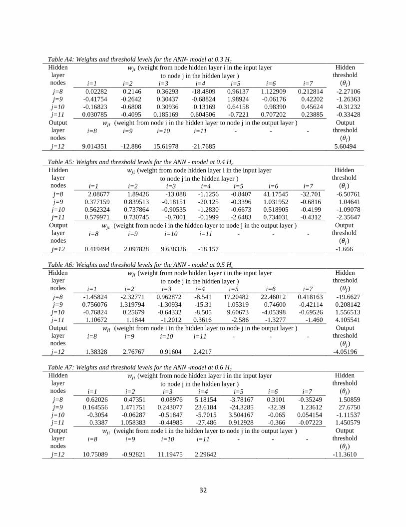
Table A4: Weights and threshold levels for the ANN- model at 0.3 Hc Hidden layer nodes


Hidden threshold

(𝜃𝑗) i=1 i=2 i=3 i=4 i=5 i=6 i=7 j=8 0.02282 0.2146 0.36293 -18.4809 0.96137 1.122909 0.212814 -2.27106 j=9 -0.41754 -0.2642 0.30437 -0.68824 1.98924 -0.06176 0.42202 -1.26363

j=10 -0.16823 -0.6808 0.30936 0.13169 0.64158 0.98390 0.45624 -0.31232 j=11 0.030785 -0.4095 0.185169 0.604506 -0.7221 0.707202 0.23885 -0.33428

Output layer nodes


(𝜃𝑗) i=8 i=9 i=10 i=11 - - -

j=12 9.014351 -12.886 15.61978 -21.7685 5.60494 Table A5: Weights and threshold levels for the ANN - model at 0.4 Hc Hidden layer nodes


Hidden threshold

(𝜃𝑗) i=1 i=2 i=3 i=4 i=5 i=6 i=7 j=8 2.08677 1.89426 -13.088 -1.1256 -0.8407 41.17545 -32.701 -6.50761 j=9 0.377159 0.839513 -0.18151 -20.125 -0.3396 1.031952 -0.6816 1.04641

j=10 0.562324 0.737864 -0.90535 -1.2830 -0.6673 0.518905 -0.4199 -1.09078 j=11 0.579971 0.730745 -0.7001 -0.1999 -2.6483 0.734031 -0.4312 -2.35647

Output layer nodes


(𝜃𝑗) i=8 i=9 i=10 i=11 - - -

j=12 0.419494 2.097828 9.638326 -18.157 -1.666 Table A6: Weights and threshold levels for the ANN - model at 0.5 Hc Hidden layer nodes


Hidden threshold

(𝜃𝑗) i=1 i=2 i=3 i=4 i=5 i=6 i=7 j=8 -1.45824 -2.32771 0.962872 -8.541 17.20482 22.46012 0.418163 -19.6627 j=9 0.756076 1.319794 -1.30934 -15.31 1.05319 0.74600 -0.42114 0.208142

j=10 -0.76824 0.25679 -0.64332 -8.505 9.60673 -4.05398 -0.69526 1.556513 j=11 1.10672 1.1844 -1.2012 0.3616 -2.586 -1.3277 -1.460 4.105541

Output layer nodes


(𝜃𝑗) i=8 i=9 i=10 i=11 - - -

j=12 1.38328 2.76767 0.91604 2.4217 -4.05196 Table A7: Weights and threshold levels for the ANN -model at 0.6 Hc Hidden layer nodes


Hidden threshold

(𝜃𝑗) i=1 i=2 i=3 i=4 i=5 i=6 i=7 j=8 0.62026 0.47351 0.08976 5.18154 -3.78167 0.3101 -0.35249 1.50859 j=9 0.164556 1.471751 0.243077 23.6184 -24.3285 -32.39 1.23612 27.6750

j=10 -0.3054 -0.06287 -0.51847 -5.7015 3.504167 -0.065 0.054154 -1.11537 j=11 0.3387 1.058383 -0.44985 -27.486 0.912928 -0.366 -0.07223 1.450579

Output layer nodes


(𝜃𝑗) i=8 i=9 i=10 i=11 - - -

j=12 10.75089 -0.92821 11.19475 2.29642 -11.3610

33

Table A8: Weights and threshold levels for the ANN -model at 0.7 Hc Hidden layer nodes


Hidden threshold

(𝜃𝑗) i=1 i=2 i=3 i=4 i=5 i=6 i=7 j=8 0.42400 0.46559 -0.1034 5.27938 -4.29611 0.05693 -0.223 1.94446 j=9 0.20791 0.18420 0.20273 5.76087 -4.2182 -0.5358 -0.031 1.80288

j=10 0.65041 2.65318 -1.61066 -38.5765 1.52342 -7.6225 0.2018 3.22180 j=11 0.111222 0.213763 -0.64653 -38.1758 2.497382 9.53468 -0.973 -4.43226

Output layer nodes


(𝜃𝑗) i=8 i=9 i=10 i=11 - - -

j=12 14.2932 -14.2761 1.782392 1.422751 -1.32971 Table A9: Weights and threshold levels for the ANN -model at 0.8 Hc Hidden layer nodes


Hidden threshold

(𝜃𝑗) i=1 i=2 i=3 i=4 i=5 i=6 i=7 j=8 0.482716 1.208346 -0.4909 5.799786 -4.74126 2.507117 -0.529 0.186043 j=9 0.715349 0.563623 0.37424 38.31441 -19.5478 -1.05955 -0.063 -1.96305

j=10 0.757585 1.53234 -1.3743 -17.3411 2.203233 -3.26635 -0.051 -0.26653 j=11 0.579219 0.284736 -1.1736 -11.4707 4.159462 7.178042 -0.853 -6.87323

Output layer nodes


(𝜃𝑗) i=8 i=9 i=10 i=11 - - -

j=12 2.574084 -1.41622 4.10681 2.846912 -2.155 Table A10: Weights and threshold levels for the ANN- model at 0.9 Hc Hidden layer nodes


Hidden Threshold

(𝜃𝑗) i=1 i=2 i=3 i=4 i=5 i=6 i=7 j=8 0.23413 0.39783 -0.1258 4.48423 -2.73151 0.31317 -0.11 0.838376 j=9 -0.72798 -2.68067 1.4830 30.1924 -0.56191 4.97414 -0.445 -2.30485

j=10 0.117852 0.00236 -0.2931 -7.23425 1.47341 0.96875 -0.165 0.709421 j=11 -0.01498 -0.12181 -0.1528 -5.9498 2.101039 0.556965 -0.072 -0.16348

Output layer nodes

𝑤𝑗𝑖 (weight from node i in the hidden layer to node j in the output layer ) i=8 i=9 i=10 i=11 - - - Output

Threshold (𝜃𝑗)

j=12 19.49644 -1.96336 -16.522 36.35604 -18.3594 Table A11: Weights and threshold levels for the ANN- model at 1 Hc Hidden layer nodes


Hidden layer

threshold (𝜃𝑗)

i=1 i=2 i=3 i=4 i=5 i=6 i=7

j=8 0.10182 0.66933 -9.45E- 4.53729 -3.77808 3.23152 -0.0659 0.35271 j=9 0.206039 0.070818 0.26018 21.02211 -6.83813 -0.35579 0.14037 -2.78455

j=10 -0.10211 0.271457 -0.1774 -26.613 4.154443 0.310213 -0.0372 5.312146 j=11 0.422038 0.611063 -0.7748 -8.54489 1.897913 -0.74841 -0.1359 -1.07541

Output layer nodes


(𝜃𝑗) i=8 i=9 i=10 i=11 - - -

j=12 4.860535 -4.40516 -3.2183 8.698041 -1.1289

restraint formulation for wall on slab at early age

Documents