RESTRICTED NEYMAN-PEARSON APPROACH

BASED SPECTRUM SENSING IN COGNITIVE RADIO

SYSTEMS

a thesis

submitted to the department of electrical and

electronics engineering

and the graduate school of engineering and sciences

of bilkent university

in partial fulfillment of the requirements

for the degree of

master of science

By

Esma Turgut

June 2012

I certify that I have read this thesis and that in my opinion it is fully adequate,

in scope and in quality, as a thesis for the degree of Master of Science.

Assist. Prof. Dr. Sinan Gezici (Supervisor)

I certify that I have read this thesis and that in my opinion it is fully adequate,

in scope and in quality, as a thesis for the degree of Master of Science.

Assist. Prof. Dr. Defne Aktas

I certify that I have read this thesis and that in my opinion it is fully adequate,

in scope and in quality, as a thesis for the degree of Master of Science.

Assoc. Prof. Dr. Ibrahim Korpeoglu

Approved for the Graduate School of Engineering and Sciences:

Prof. Dr. Levent OnuralDirector of Graduate School of Engineering and Sciences

ii

ABSTRACT

RESTRICTED NEYMAN-PEARSON APPROACH

BASED SPECTRUM SENSING IN COGNITIVE RADIO

SYSTEMS

Esma Turgut

M.S. in Electrical and Electronics Engineering

Supervisor: Assist. Prof. Dr. Sinan Gezici

June 2012

Over the past decade, the demand for wireless technologies has increased enor-

mously, which leads to a perceived scarcity of the frequency spectrum. Mean-

while, static allocation of the frequency spectrum leads to under-utilization of

the spectral resources. Therefore, dynamic spectrum access has become a ne-

cessity. Cognitive radio has emerged as a key technology to solve the conflicts

between spectrum scarcity and spectrum under-utilization. It is an intelligent

wireless communication system that is aware of its operating environment and

can adjust its parameters in order to allow unlicensed (secondary) users to ac-

cess and communicate over the frequency bands assigned to licensed (primary)

users when they are inactive. Therefore, cognitive radio requires reliable spec-

trum sensing techniques in order to avoid interference to primary users. In this

thesis, the spectrum sensing problem in cognitive radio is studied. Specifically,

the restricted Neyman-Pearson (NP) approach, which maximizes the average de-

tection probability under the constraints on the minimum detection and false

alarm probabilities, is applied to the spectrum sensing problem in cognitive ra-

dio systems in the presence of uncertainty in the prior probability distribution of

iii

primary users’ signals. First, we study this problem in the presence of Gaussian

noise and assume that primary users’ signals are Gaussian. Then, the problem

is reconsidered for non-Gaussian noise channels. Simulation results are obtained

in order to compare the performance of the restricted NP approach with the

existing methods such as the generalized likelihood ratio test (GLRT) and en-

ergy detection. The restricted NP approach outperforms energy detection in all

cases. It is also shown that the restricted NP approach can provide important

advantages over the GLRT in terms of the worst-case detection probability, and

sometimes in terms of the average detection probability depending on the situ-

ation in the presence of imperfect prior information for Gaussian mixture noise

channels.

Keywords: Cognitive radio, detection, spectrum sensing, Neyman-Pearson.

iv

OZET

BILISSEL RADYO SISTEMLERINDE KISITLI

NEYMAN-PEARSON YAKLASIMI TABANLI SPEKTRUM

SEZME

Esma Turgut

Elektrik ve Elektronik Muhendisligi Bolumu Yuksek Lisans

Tez Yoneticisi: Yrd. Doc. Dr. Sinan Gezici

Haziran 2012

Gectigimiz on yıl icinde kablosuz teknolojilere olan talep, frekans spektru-

munda farkedilebilir bir kıtlıga yol acacak sekilde fazlasıyla artmıstır. Aynı za-

manda, frekans spektrumunun statik tahsisi spektrumun verimsiz kullanımına yol

acmıstır. Dolayısıyla dinamik spektrum erisimi bir zorunluluk haline gelmistir.

Bilissel radyo, spektrum kıtlıgı ve spektrumun verimsiz kullanımı arasındaki

catısmaları cozmek icin anahtar teknoloji olarak ortaya cıkmıstır. Bilissel radyo

lisanssız (ikincil) kullanıcıların lisanslı (birincil) kullanıcılara ayrılan frekans

bandlarına onlar aktif degilken erisip iletisim kurabilmelerine izin vermek icin

parametrelerini ayarlayabilen ve calısma ortamının farkında olan, akıllı bir

kablosuz iletisim sistemidir. Bilissel radyo, birincil kullanıcılarla girisimi en-

gellemek amacıyla guvenilir spektrum sezme tekniklerine ihtiyac duyar. Bu

tezde, bilissel radyolardaki spektrum sezme konusu calısılmaktadır. Ozel olarak,

minimum tespit ve yanlıs alarm olasılıkları uzerindeki kısıtlamalar altında

ortalama tespit olasılıgını maksimuma cıkaran kısıtlı Neyman-Pearson (NP)

iv

yaklasımı, birincil kullanıcıların sinyallerinin onsel olasılık dagılımındaki belir-

sizligin varlıgında bilissel radyolardaki spektrum sezme problemine uygulanmak-

tadır. Ilk olarak Gauss gurultu varlıgında bu problem incelenmekte ve birin-

cil kullanıcıların sinyallerinin Gauss dagılımı oldugu varsayılmaktadır. Daha

sonra, Gauss olmayan gurultu kanalları icin problem tekrar ele alınmaktadır.

Kısıtlı NP yaklasımının performansını, genellestirilmis olabilirlik oranı testi

(GLRT) ve enerji algılama gibi varolan metodların performansıyla karsılastırmak

icin simulasyon sonucları elde edilmektedir. Her iki gurultu kanalında da

kısıtlı NP yaklasımı enerji algılama metodunu geride bırakmaktadır. Ayrıca,

Gauss karısım gurultu kanalları icin onsel bilgi eksikliginin varlıgında kısıtlı NP

yaklasımı, en kotu durumdaki tespit olasılıgı acısından ve bazen de duruma

baglı olarak ortalama tespit olasılıgı acısından GLRT uzerinde onemli avanta-

jlar saglayabilmektedir.

Anahtar Kelimeler: Bilissel radyo, sezim, spektrum sezme, Neyman-Pearson.

v

ACKNOWLEDGMENTS

First and foremost I would like to express my sincere gratitude to my advisor,

Assist. Prof. Dr. Sinan Gezici of the Electrical and Electronics Engineering

Department at Bilkent University, for his invaluable guidance, continuous en-

couragement, enduring patience, immense knowledge and constant support. I

appreciate his consistent support from the first day I applied to graduate pro-

gram to these concluding moments. I also sincerely thanks for the time spent

proofreading and correcting my many mistakes.

I also would like to thank the other members of my thesis committee, Assist.

Prof. Dr. Defne Aktas of the Electrical and Electronics Engineering Department

and Assoc. Prof. Dr. Ibrahim Korpeoglu of Computer Engineering Department,

both at Bilkent University for their suggestions, insightful comments and hard

questions.

I also would like to thank to TUBITAK (Scientific and Technological Research

Council of Turkey) for their financial support (BIDEB-2210 Fellowship) during

my master study.

Finally, I would like to express my deepest appreciation to my mother and

father for their unconditional love, devotion and support throughout my life, and

also to my brother, sister, mother in law and father in law for their encouragement

throughout my study. And my most special thanks to my husband, for his love,

support, patience, and encouragement through my academic life.

v

Contents

1 INTRODUCTION AND BACKGROUND 1

1.1 Introduction . . . . . . . . . . . . . . . . . . . . . . . . . . . . . . 1

1.2 Spectrum Sensing . . . . . . . . . . . . . . . . . . . . . . . . . . . 5

1.2.1 Spectrum Sensing Problem . . . . . . . . . . . . . . . . . . 7

1.2.2 Matched Filtering . . . . . . . . . . . . . . . . . . . . . . . 8

1.2.3 Cyclostationary Feature Detection . . . . . . . . . . . . . . 8

1.2.4 Energy Detection . . . . . . . . . . . . . . . . . . . . . . . 9

1.3 Thesis Organization and Contributions . . . . . . . . . . . . . . . 10

2 Restricted Neyman-Pearson Approach 12

2.1 Background Information . . . . . . . . . . . . . . . . . . . . . . . 12

2.2 Restricted Neyman-Pearson Approach . . . . . . . . . . . . . . . 15

2.2.1 Problem Formulation . . . . . . . . . . . . . . . . . . . . . 15

2.2.2 Characterization of Optimal Decision Rule . . . . . . . . . 17

2.2.3 Algorithm . . . . . . . . . . . . . . . . . . . . . . . . . . . 19

vi

3 Application of the Restricted Neyman-Pearson Approach to

Spectrum Sensing in Cognitive Radio 21

3.1 Spectrum Sensing in the Presence of Gaussian Noise . . . . . . . . 22

3.1.1 Restricted NP Approach . . . . . . . . . . . . . . . . . . . 23

3.1.2 GLRT Approach . . . . . . . . . . . . . . . . . . . . . . . 24

3.1.3 Energy Detection Approach . . . . . . . . . . . . . . . . . 25

3.2 Spectrum Sensing over Non-Gaussian Channels . . . . . . . . . . 26

3.2.1 Single Observation Case . . . . . . . . . . . . . . . . . . . 26

3.2.2 Multiple Observations Case . . . . . . . . . . . . . . . . . 28

4 NUMERICAL RESULTS 29

4.1 Simulation Results for Spectrum Sensing in the Presence of Gaus-

sian Noise . . . . . . . . . . . . . . . . . . . . . . . . . . . . . . . 30

4.2 Simulation Results for Spectrum Sensing over Non-Gaussian

Channels . . . . . . . . . . . . . . . . . . . . . . . . . . . . . . . . 35

4.2.1 Single Observation Case . . . . . . . . . . . . . . . . . . . 35

4.2.2 Multiple Observations Case . . . . . . . . . . . . . . . . . 41

5 CONCLUSIONS 44

APPENDIX 46

A Calculation of Mean and Variance of X 46

vii

List of Figures

1.1 The NTIA’s frequency allocation chart [1]. . . . . . . . . . . . . . 2

1.2 Measurement of 0-6 GHz spectrum utilization in downtown Berke-

ley, CA [2]. . . . . . . . . . . . . . . . . . . . . . . . . . . . . . . 3

1.3 Temporal variation of the spectrum utilization (0-2.5 GHz) in

downtown Berkeley, CA [2]. . . . . . . . . . . . . . . . . . . . . . 3

1.4 Cognitive cycle [3]. . . . . . . . . . . . . . . . . . . . . . . . . . . 4

1.5 Three main types of spectrum sensing techniques [4]. . . . . . . . 10

4.1 Detection probability versus θ for the three approaches for a = 0.5,

b = 1, σ2n = 0.5, N = 1 and α = 0.1. . . . . . . . . . . . . . . . . . 31

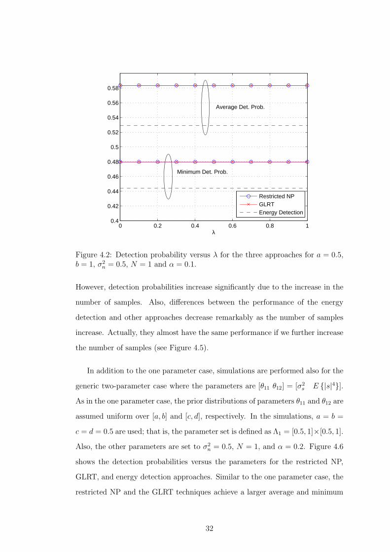
4.2 Detection probability versus λ for the three approaches for a = 0.5,

b = 1, σ2n = 0.5, N = 1 and α = 0.1. . . . . . . . . . . . . . . . . . 32

4.3 Detection probability versus θ for the three approaches for a = 0.5,

b = 1, σ2n = 0.5, N = 5 and α = 0.1. . . . . . . . . . . . . . . . . . 33

4.4 Detection probability versus λ for the three approaches for a = 0.5,

b = 1, σ2n = 0.5, N = 5 and α = 0.1. . . . . . . . . . . . . . . . . . 33

viii

4.5 Detection probability versus θ for the three approaches for a = 0.5,

b = 1, σ2n = 0.5, N = 10 and α = 0.1. . . . . . . . . . . . . . . . . 34

4.6 Detection probability versus θ11 and θ12 for the three approaches

for σ2n = 0.5, N = 1 and α = 0.2. The restricted NP and the

GLRT approaches have almost the same performance, while the

energy detection results in lower detection probability for most

parameter values. . . . . . . . . . . . . . . . . . . . . . . . . . . . 35

4.7 Detection probability versus θ for the restricted NP and GLRT

approaches, where the parameters of the Gaussian mixture noise

are set to Nm = 4, ν1 = ν4 = 0.3, ν2 = ν3 = 0.2, µ1 = −µ4 = 0.9,

µ2 = −µ3 = 0.5, and ǫi = 0.1 ∀ i. . . . . . . . . . . . . . . . . . . 37

4.8 Detection probability versus λ for the restricted NP, GLRT and

ED approaches, where the parameters of the Gaussian mixture

noise are set to Nm = 4, ν1 = ν4 = 0.3, ν2 = ν3 = 0.2, µ1 = −µ4 =

0.9, µ2 = −µ3 = 0.5, and ǫi = 0.1 ∀ i. . . . . . . . . . . . . . . . . 37

4.9 Detection probability versus θ for the restricted NP and GLRT

approaches, where the parameters of the Gaussian mixture noise

are set to Nm = 3, ν1 = ν3 = 0.25, ν2 = 0.5, µ1 = −µ3 = 1,

µ2 = 0, and ǫi = 0.2 ∀ i. . . . . . . . . . . . . . . . . . . . . . . . 38

4.10 Detection probability versus λ for the restricted NP, GLRT and

ED approaches, where the parameters of the Gaussian mixture

noise are set to Nm = 3, ν1 = ν3 = 0.25, ν2 = 0.5, µ1 = −µ3 = 1,

µ2 = 0, and ǫi = 0.2 ∀ i. . . . . . . . . . . . . . . . . . . . . . . . 39

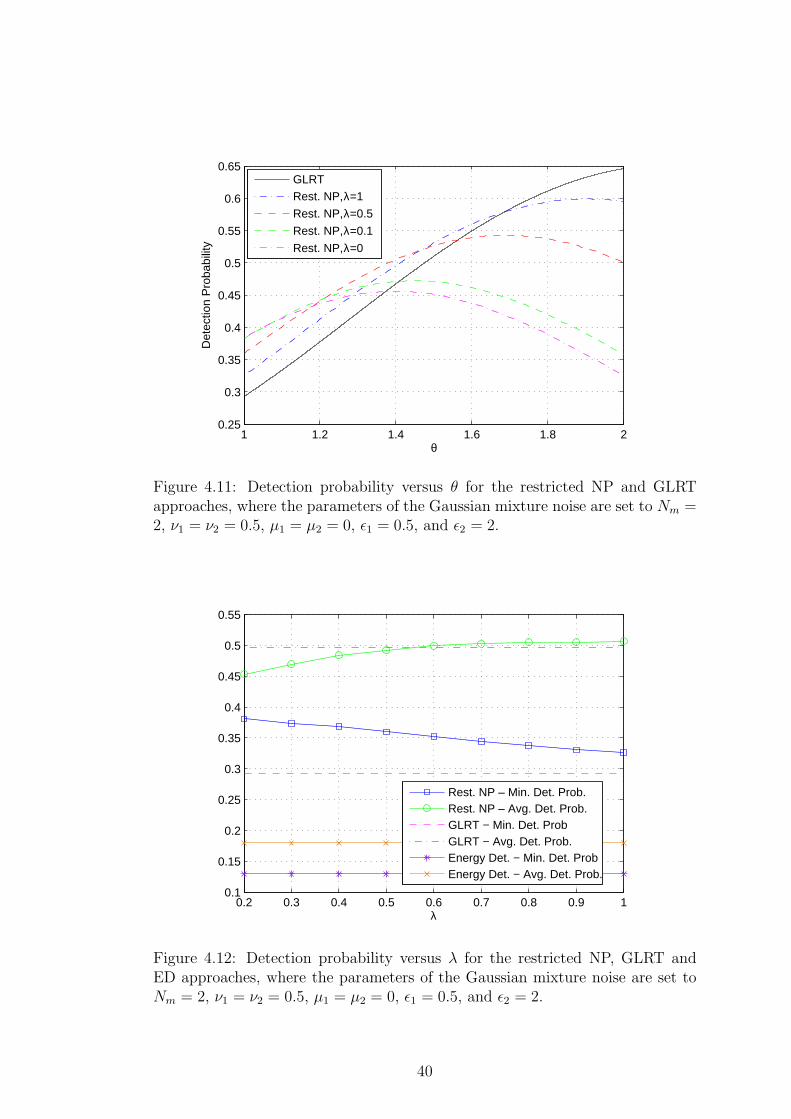
4.11 Detection probability versus θ for the restricted NP and GLRT

approaches, where the parameters of the Gaussian mixture noise

are set to Nm = 2, ν1 = ν2 = 0.5, µ1 = µ2 = 0, ǫ1 = 0.5, and ǫ2 = 2. 40

ix

4.12 Detection probability versus λ for the restricted NP, GLRT and

ED approaches, where the parameters of the Gaussian mixture

noise are set to Nm = 2, ν1 = ν2 = 0.5, µ1 = µ2 = 0, ǫ1 = 0.5, and

ǫ2 = 2. . . . . . . . . . . . . . . . . . . . . . . . . . . . . . . . . . 40

4.13 Detection probability versus θ for the restricted NP, GLRT, and

energy detection approaches for M = 5. . . . . . . . . . . . . . . . 41

4.14 Detection probability versus λ for the restricted NP, GLRT, and

energy detection approaches for M = 5. For the energy detector,

the minimum detection probability is 0.808, which is not shown

in the figure. . . . . . . . . . . . . . . . . . . . . . . . . . . . . . . 42

4.15 Detection probability versus θ for the GLRT approach for various

numbers of observations. . . . . . . . . . . . . . . . . . . . . . . . 43

4.16 Detection probability versus θ for the energy detection approach

for various numbers of observations. . . . . . . . . . . . . . . . . . 43

x

List of Tables

4.1 Gaussian mixture noise parameters. . . . . . . . . . . . . . . . . . 36

xi

Dedicated to my husband Emrah . . .

Chapter 1

INTRODUCTION AND

BACKGROUND

1.1 Introduction

In the past decade, wireless technologies have grown rapidly and the spectrum

resources have faced difficulties in meeting the increasing demand [5]. Since

spectrum is an unexpandable natural resource, increasing wireless services such

as mobile phones, 3G and 4G mobile services, wireless internet and many oth-

ers lead to spectrum scarcity [5]. In traditional spectrum allocation, frequency

bands are assigned to specific licensed users and other users cannot use those

bands even if the licensed users are idle. The National Telecommunication and

Information Administration’s (NTIA) chart of spectrum frequency allocations in

Figure 1.1 indicates that within the current spectrum regulatory framework, all of

the frequency bands are exclusively allocated to specific services and the Federal

Communications Commission (FCC) does not allow violation from unlicensed

users because of its regulations. However, actual measurements of spectrum uti-

lization show that many assigned bands are largely unoccupied most of the time.

1

Figure 1.1: The NTIA’s frequency allocation chart [1].

Figure 1.2 shows the measurement of 0-6 GHz spectrum utilization taken by the

Berkeley Wireless Research Center (BWRC) in downtown Berkeley, CA. As can

be seen, spectrum is utilized more intensely at frequencies below 3 GHz, while

spectrum is under-utilized in 3-6 GHz bands [2]. Moreover, measurements taken

over 10 minutes in the same Berkeley location (Figure 1.3) indicate that there

are also temporal gaps in the spectrum usage even in the 0 to 2.5 GHz band,

which is considered to be very crowded. Recent measurements taken in the US

and the world have shown similar results. These measurements lead to the seri-

ous questioning of the convenience of the current regulatory regime and possibly

provide the opportunity to solve the spectrum scarcity problem. According to

a recent report by the USA Federal Communications Commission (FCC), fixed

spectrum allocation leads to utilization of spectrum very inefficiently in almost

all currently deployed frequency bands and, they therefore recommend allowing

the secondary users to fill the available spectrum holes [6].

Cognitive radio, first proposed in 1999 in [7], has emerged as a promising ap-

proach to solve the conflicts between spectrum under-utilization and spectrum

scarcity. In other words, cognitive radio was proposed to improve spectrum uti-

lization via opportunistic spectrum sharing. The basic idea behind the cognitive

2

Figure 1.2: Measurement of 0-6 GHz spectrum utilization in downtown Berkeley,CA [2].

Figure 1.3: Temporal variation of the spectrum utilization (0-2.5 GHz) in down-town Berkeley, CA [2].

3

Figure 1.4: Cognitive cycle [3].

radio is allowing unlicensed (secondary) users to access and communicate over

the frequency bands assigned to licensed (primary) users when they are inactive.

Hence, a cognitive radio may be defined as an intelligent wireless communica-

tion system that is aware of its environment and can change its transmission

and reception parameters based on interaction with the environment in which

it operates in order to have reliable communication without interfering with the

primary users and optimize spectrum usage.

Cognitive radio has two main characteristics: cognitive capability and re-

configurability [3]. Firstly, cognitive capability refers to the ability of the radio

technology to capture or sense the information from its radio environment. This

ability is useful to identify the spectrum holes at a specific time or location. To

do this cognitive radio has to perform some tasks shown in Figure 1.4, which is re-

ferred as the cognitive cycle. The cognitive cycle has three main steps: spectrum

sensing, spectrum analysis, and spectrum decision. Secondly, reconfigurability

means adjusting operating parameters according to radio environment. There

are several reconfigurable parameters such as operating frequency, modulation,

transmission power, and communication technology.

4

In the next the section spectrum sensing task is discussed in detail.

1.2 Spectrum Sensing

In cognitive radio systems, one of the most important tasks is spectrum sensing,

i.e., detection of the presence or absence of primary users. Reliable and fast

spectrum sensing is important because secondary users should cause little in-

terference to primary users while achieving higher utilization of spectrum holes.

Spectrum sensing is a very challenging task due to several reasons [8]. One of

them is low signal to noise ratio (SNR). For example, if the transmitted signal

of a primary user is in an deep fade, then detection becomes very hard for a

secondary user even if the primary and secondary users are very close to each

other. A practical scenario is that the received SNR is less than -20 dB for a

secondary user several hundred meters away from a wireless microphone which

transmits with a power less than 50 mW and a bandwidth less than 200 kHz [8].

Secondly, multipath fading and time dispersion of the wireless channels are the

other problems which make sensing complicated. First one may cause great fluc-

tuations in signal power and second one may make coherent detection unreliable

[8]. Thirdly, noise power uncertainty is another problem that makes spectrum

sensing a challenging task and it has been heavily studied in recent years such

as in [9], [10], [11].

The spectrum sensing problem has been studied extensively and it has become

a very active research area in recent years. Many sensing methods have been

proposed to identify the presence of signal transmission. Sensing methods can

be classified into three categories according to their requirements [8]:

(1) Methods requiring both source signal and noise power information (non

blind detection)

5

(2) Methods requiring only noise power information (semi blind detection)

(3) Methods requiring no information on signal and noise power (totally blind

detection)

The first category includes methods such as likelihood ratio test [12], matched

filtering [12], [13], and cyclostationary feature detection [14], [15], [16], [17]. En-

ergy detection [13], [12], [18] and wavelet-based sensing [19] methods belong to

the second category. On the other hand, sensing techniques like eigenvalue-based

sensing, covariance-based sensing and blindly combined energy detection are in-

cluded in the third category.

Among all sensing techniques energy detection, matched filtering and cyclo-

stationary detection are the most popular ones. Choice of a spectrum sensing

technique depends on available information about primary signals as mentioned

above. The matched filter provides the best performance among these three

methods but it needs complete prior knowledge about the primary user signal.

If the primary user signal exhibits certain periodicity in the mean and auto-

correlation, then cognitive radio uses cyclostationary feature detection. On the

other hand, energy detection is the optimal and simplest one if there is limited

information on structure of primary users’ signal [20]. However, the energy de-

tector needs to know the noise variance for proper operation. In practice, it is

difficult to know noise variance accurately and uncertainty in the noise variance

can degrade the performance of the energy detector dramatically.

In the following subsections, first a generic formulation of the spectrum sens-

ing problem is provided then these three popular sensing methods are discussed

in detail.

6

1.2.1 Spectrum Sensing Problem

Spectrum sensing is based on a well-known technique called signal detection.

Signal detection is a method used to identify the presence of a signal in a noisy

environment [21]. The signal detection problem can be formulated as a sim-

ple hypothesis-testing problem in which we assume that there are two possible

hypotheses, H0 and H1 [22];

x(n) =

w(n), H0

s(n) + w(n), H1

where x(n) is the received signal at the secondary user, s(n) is the transmitted

signal of the primary user and w(n) is noise (not necessarily white Gaussian

noise) of variance σ2. H0 and H1 are the noise-only and the signal plus noise

hypotheses, respectively. In other words, H0 declares absence the of the signal

while H1 points out the presence of the signal. The hypotheses H0 and H1 are

sometimes referred as the null and alternative hypotheses, respectively. There

are four possible cases for the detected signal [21]:

1) Declaring H0 when H0 is true (H0|H0)

2) Declaring H1 when H1 is true (H1|H1): Detection

3) Declaring H0 when H1 is true (H0|H1): Miss detection

4) Declaring H1 when H0 is true (H1|H0): False alarm

The primary aim of signal detection is to increase the probability of detection

Pd = P (H1|H1) and decrease the probability of false alarm Pf = P (H1|H0) as

much as possible. Miss detections and false alarms are important issues for

spectrum sensing since the first one results in interference with primary user

signals and the second one is desired to be as low as possible so that secondary

7

users can utilize all possible transmission opportunities (i.e., can have high data

rates).

1.2.2 Matched Filtering

The matched filter is the optimal detector in the stationary Gaussian noise if

the primary user signal is known to the secondary user, since it maximizes the

received SNR [3]. Although it is computationally simple and due to coherency

it requires less time to achieve high processing gain, a matched filter requires

a priori knowledge of the primary user signal such as modulation type and or-

der, pulse shape, and packet format and also requires knowledge on the channel

responses from the primary user to the receiver [3], [23]. If this information is

not accurate, then performance of the matched filter significantly degrades. In

practice, cognitive radios do not know the signal perfectly so this technique is

not well-suited for spectrum sensing in cognitive radio systems.

1.2.3 Cyclostationary Feature Detection

Another spectrum sensing method is cyclostationary feature detection. Modu-

lated signals are in general coupled with sine wave carriers, pulse trains, repeating

spreading, hopping sequences, or cyclic prefixes, which result in built-in periodic-

ity [3]. Mean and autocorrelation of these signals exhibit periodicity so they are

classified as cyclostationary. We can detect these features by analyzing a spec-

tral correlation function. On the other hand, noise is wide-sense stationary with

no correlation. Hence, the spectral correlation function differentiates the noise

energy from the modulated signal energy. Therefore, cyclostationary feature de-

tectors are robust to noise uncertainty and work even in very low SNR region

unlike the energy detectors [24], [25]. Hence, FCC has suggested cyclostationary

8

detectors as a useful alternative to enhance the detection sensitivity in cognitive

radio networks [6].

In cyclostationary feature detection, the period of the primary signal should

be known as a priori knowledge. This can be possible in the early stage of a

cognitive radio application, because only limited spectrum bands, such as TV

bands, are open to cognitive radio users and the characteristics of the primary

signals are well known to the secondary users. When CRs are allowed to use

wide-band spectrum in the future, the periods of some modulated primary sig-

nals may not be known by the secondary users. In such a situation, too much

effort is needed to search for cyclic frequencies which means huge computational

complexity and the loss of the ability to differentiate the primary signal from the

interference that is also cyclostationary [25]. Also, this type detection can only

be applicable for few primary signals with such characteristics.

1.2.4 Energy Detection

If only the noise power is known to the receiver, the optimal detector is the

energy detector [20]. The detection mechanism of an energy detector is simple as

depicted in Figure 1.5. The detector first computes the signal energy and then

compares it to a predetermined threshold value to decide whether the primary

signal is present or not. This threshold is set according to the desired probability

of false alarm. Since it is easy to implement and less expensive when compared

to other methods, the recent work on detection of the primary user has generally

adopted the energy detector [26], [20]. One drawback of the energy detector is

that it is very sensitive to uncertainty in the noise power. If the noise power is

not perfectly known, the energy detector performs poorly. Another one is that

the energy detector can only determine the presence of the signal not its type or

source. Hence, false alarm probability can increase due to unintended signals.

9

Figure 1.5: Three main types of spectrum sensing techniques [4].

In practice, energy detection is especially appropriate for wide-band spectrum

sensing. Wide-band spectrum sensing is usually done in two steps. In the first

step, low-complexity energy detection is applied to search for possible idle sub

bands and then more advanced spectrum sensing techniques such as cyclostation-

ary feature detection are employed to determine whether sub band candidates

are available or not for secondary usage [25].

1.3 Thesis Organization and Contributions

In this thesis, we study the spectrum sensing problem in cognitive radio systems.

Our main contribution is developing an application of the restricted NP algorithm

to the spectrum sensing problem in cognitive radios. The important point is that

the restricted NP approach assumes neither the perfect knowledge of the prior

information nor the absence of it. This is usually the case in cognitive radios,

i.e., some information about the prior distribution is available in many cases

but that information is not perfect most of the time. Therefore, we take into

account the uncertainty in the prior distribution of primary signals available

to cognitive radio using the restricted NP approach in spectrum sensing. The

employed restricted NP approach maximizes the average detection probability

10

while the minimum detection probability under the constraints that the minimum

detection probability should be larger than a predefined value and that the false-

alarm probability should be less than a significance level.

The rest of the thesis is organized as follows:

In Chapter 2, we first provide background information about common hy-

pothesis testing techniques, and mention the techniques which take into account

partial prior information. Second, the description of the restricted NP approach

is provided [27]. Then, we explain how the optimal decision rule is found. Finally,

a three step algorithm for the restricted NP approach is presented.

In Chapter 3, we investigate how the generic restricted NP approach can

be applied to the spectrum sensing problem in cognitive radio systems. First,

Gaussian noise channels are considered. In the presence of Gaussian noise, first

Gaussian primary user signals are taken into consideration. Then, we reconsider

the problem when no special distributions for primary user signals are assumed.

We continue this chapter by presenting applications of the restricted NP approach

to the spectrum sensing problem over non-Gaussian channels. For each scheme,

we also provide the formulation of the GLRT and energy detection approaches

in order to evaluate the performance of the restricted NP approach.

In Chapter 4, numerical results for the restricted NP method, and existing

GLRT and energy detection approaches are provided. We present simulation

results for various scenarios first in the presence of Gaussian noise, then in the

presence of Gaussian mixture noise, respectively.

In Chapter 5, the main ideas of the thesis are summarized and some possible

future works are proposed to extend this research.

11

Chapter 2

Restricted Neyman-Pearson

Approach

2.1 Background Information

As mentioned in the previous section, spectrum sensing is one of the most impor-

tant tasks in cognitive radio systems. That is, secondary users should detect the

presence of primary users in order to avoid interference and determine spectrum

holes. Since spectrum sensing is based on signal detection, it is important to

apply the optimal detection rule. For any given decision problem, there are a

number of possible decision strategies that can be applied. Bayesian, minimax

and Neyman Pearson hypothesis testings are three most common approaches for

the formulation of testing [22]. The Bayesian approach assumes that perfect

prior knowledge is available whereas the minimax approach completely ignores

the prior information [28]. Therefore, Bayesian and minimax decision rules are

the two extreme cases of prior information. In the Bayesian framework, all forms

of uncertainty are represented by a prior probability distribution, and posterior

probabilities are used to make a decision. If the prior probabilities are unknown,

12

then the Bayesian approach is not appropriate since it is unlikely that a single de-

cision rule would minimize the average risk for every possible prior distribution.

Hence, in this case the minimax approach is an alternative decision rule which

minimizes the maximum of risk functions defined over the parameter space [22].

In practice, complete prior information is available in rare situations and usually

only partial prior information is accessible [29], [30]. Absence of exact prior in-

formation causes degradation in the performance of the Bayesian approach. On

the other hand, ignoring the partial prior information is the primary reason for

poor performance of the minimax approach. Therefore, various approaches that

take partial information into account have been proposed such as [29], [30], [31],

[32] and [33].

The restricted Bayes decision rule is one of the decision rules that take par-

tial information into account. It minimizes the Bayes risk under a constraint

on the individual conditional risks [34]. The value of the constraint is deter-

mined according to the amount of uncertainty in the prior information, so the

restricted Bayesian approach is a compromise between the Bayesian and minimax

approaches [30]. Since uncertainty measurement is necessary in the calculation

of the Bayes risk and imposing a constraint on the conditional risks is a non-

probabilistic description of uncertainty, the restricted Bayes approach combines

probabilistic and non-probabilistic descriptions of uncertainty. In [27], the idea

of the restricted Bayes approach is adopted to the NP framework, which is ex-

plained in detail in the next paragraph.

In the NP approach, the goal is to maximize the detection probability un-

der a constraint on the false-alarm probability by deciding between the null and

alternative hypotheses [22]. In some cases the null hypothesis may be compos-

ite, and the false-alarm constraint for all possible distributions can be applied

in such situations [35], [36]. On the other hand, when alternative hypothesis

is composite, there are various approaches to this problem. One of them is to

13

search for a uniformly most powerful (UMP) test which maximizes the detection

probability by imposing false-alarm constraints for all possible probability distri-

butions under the alternative hypothesis. However, finding a UMP test is very

exceptional in many cases [22]. Hence, other approaches have been proposed.

In one approach, for example, the average detection probability is maximized

under the false-alarm constraint [37], [38], [39]. In this case, a prior distribution

of the parameter under the alternative hypothesis should be known to be able

to calculate average detection probability. This max-mean approach is like the

classical NP approach. On the other hand, the max-min approach, the aim of

which is to maximize the minimum detection probability under the false-alarm

constraint, can be applied if a prior distribution is not available [35], [36]. The

max-min approach is conservative because its solution is a NP decision rule cor-

responding to the least-favorable distribution of the unknown parameter under

the alternative hypothesis.

In [27], the restricted NP approach is studied which can be considered as an

application of the restricted Bayes approach to the NP framework [34], [30]. This

approach maximizes the average detection probability under the constraints that

the minimum detection probability should be larger than a predefined value and

that the false-alarm probability should be less than a significance level. Thus, the

uncertainty in the prior distribution information under the alternative hypothesis

is considered, and the constraint on the minimum (worst-case) detection proba-

bility is adjusted depending on the amount of uncertainty [27]. The classical NP

(max-mean) and the max-min criteria are the special cases of the restricted NP

criterion.

In this chapter, the restricted NP approach is presented, and then its appli-

cation to the spectrum sensing problem in cognitive radio systems is provided in

the next chapter.

14

2.2 Restricted Neyman-Pearson Approach

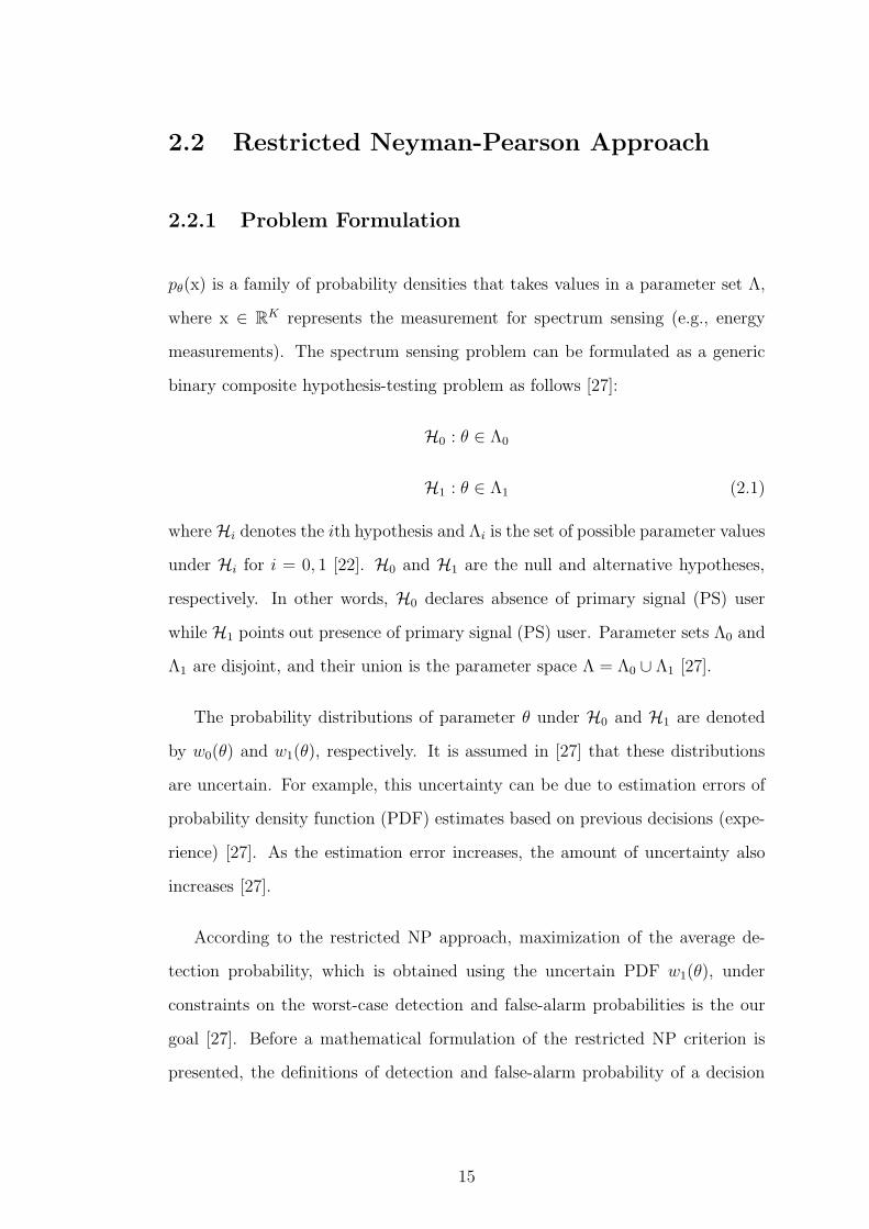
2.2.1 Problem Formulation

pθ(x) is a family of probability densities that takes values in a parameter set Λ,

where x ∈ RK represents the measurement for spectrum sensing (e.g., energy

measurements). The spectrum sensing problem can be formulated as a generic

binary composite hypothesis-testing problem as follows [27]:

H0 : θ ∈ Λ0

H1 : θ ∈ Λ1 (2.1)

whereHi denotes the ith hypothesis and Λi is the set of possible parameter values

under Hi for i = 0, 1 [22]. H0 and H1 are the null and alternative hypotheses,

respectively. In other words, H0 declares absence of primary signal (PS) user

while H1 points out presence of primary signal (PS) user. Parameter sets Λ0 and

Λ1 are disjoint, and their union is the parameter space Λ = Λ0 ∪ Λ1 [27].

The probability distributions of parameter θ under H0 and H1 are denoted

by w0(θ) and w1(θ), respectively. It is assumed in [27] that these distributions

are uncertain. For example, this uncertainty can be due to estimation errors of

probability density function (PDF) estimates based on previous decisions (expe-

rience) [27]. As the estimation error increases, the amount of uncertainty also

increases [27].

According to the restricted NP approach, maximization of the average de-

tection probability, which is obtained using the uncertain PDF w1(θ), under

constraints on the worst-case detection and false-alarm probabilities is the our

goal [27]. Before a mathematical formulation of the restricted NP criterion is

presented, the definitions of detection and false-alarm probability of a decision

15

rule are given in [27] as follows:

PD(φ; θ) ,∫

Γ

φ(x)pθ(x)dx, for θ ∈ Λ1 (2.2)

PF (φ; θ) ,∫

Γ

φ(x)pθ(x)dx, for θ ∈ Λ0 (2.3)

where Γ represents the observation space, and φ(x) denotes a generic decision rule

(detector) that maps x into a real number in [0, 1], representing the probability

of selecting H1 [22]. Then, the formulation of the restricted NP criterion is the

following optimization problem [27]:

maxφ

∫

Λ1

PD(φ; θ)w1(θ)dθ (2.4)

subject to PD(φ; θ) ≥ β, ∀θ ∈ Λ1 (2.5)

PF (φ; θ) ≤ α, ∀θ ∈ Λ0 (2.6)

where α is the false-alarm constraint, and β is the design parameter to compen-

sate for the uncertainties in w1(θ). In other words, a restricted NP decision rule

is a rule that maximizes the average detection probability (obtained based on

the prior distribution estimate w1(θ)) under the constraints on the worst-case

detection and false-alarm probabilities. Worst-case detection probability should

be higher than β, and false-alarm probability should be smaller than α.

Max-min and classical NP approaches are two special cases of the formulation

in (2.4)-(2.6) [27]. In the case of full uncertainty in w1(θ) (no prior information),

the restricted NP problem reduces to the max-min problem and the following

problem is considered [27]:

maxφ

minθ∈Λ1

PD(φ; θ)

subject to PF (φ; θ) ≤ α, ∀θ ∈ Λ0 (2.7)

On the other hand, in the case of no uncertainty in w1(θ) (perfect prior informa-

tion), the restricted NP problem turns into the classical NP problem, which can

16

be presented as follows [27]:

maxφ

P avgD (φ)

subject to PF (φ; θ) ≤ α, ∀θ ∈ Λ0 (2.8)

where P avgD (φ) ,

∫Λ1

PD(φ; θ)w1(θ)dθ defines the average detection probability.

According to the theoretical results in [34], [30], we can show that the optimal

solution to (2.4)-(2.6) is in the form of an NP decision rule corresponding to the

least-favorable distribution [27]. The least-favorable distribution can be obtained

by combining the uncertain PDF w1(θ) and any other PDF µ(θ) as follows [27]:

v(θ) = λw1(θ) + (1− λ)µ(θ) (2.9)

and the PDF v(θ) that corresponds to the minimum average detection probability

can be found [27].

2.2.2 Characterization of Optimal Decision Rule

A detailed formulation of the restricted NP algorithm can be obtained by em-

ploying the definitions in (2) and (3) to reformulate the problem in ((2.4)-(2.6)

as [27]

maxφ

∫

Γ

φ(x)p1(x)dx (2.10)

subject to minθ∈Λ1

∫

Γ

φ(x)pθ(x)dx ≥ β (2.11)

maxθ∈Λ0

∫

Γ

φ(x)pθ(x)dx ≤ α (2.12)

where p1(x) ,∫Λ1

pθ(x)w1(θ)dθ is the PDF of the observation under H1, which is

obtained based on the prior distribution estimate w1(θ). The problem in (2.10)-

(2.12) can be represented alternatively as follows [27]

maxφ

λ

∫

Γ

φ(x)p1(x)dx + (1− λ) minθ∈Λ1

∫

Γ

φ(x)pθ(x)dx

subject tomaxθ∈Λ0

∫

Γ

φ(x)pθ(x)dx ≤ α (2.13)

17

where 0 ≤ λ ≤ 1 is a design parameter that is selected according to β [27]. As

a special case, if λ = 0 then the restricted NP reduces to max-min problem.

Similarly, if λ = 1 then it reduces to classical NP problem [27].

If the parameter space for H0 is specified as Λ0 = 0, then (2.13) becomes

maxφ

λ

∫

Γ

φ(x)p1(x)dx + (1− λ) minθ∈Λ1

∫

Γ

φ(x)pθ(x)dx

subject to

∫

Γ

φ(x)p0(x)dx ≤ α (2.14)

Based on NP lemma [22], we can show that the solution of (2.14) is in the

form of a likelihood ratio test (LRT) as follows [27]:

φ∗(x) =

1,

∫Λ1

pθ(x)v(θ)dθ ≥ ηp0(x)

0,∫Λ1

pθ(x)v(θ)dθ < ηp0(x)(2.15)

where the threshold η is chosen such that the false-alarm rate is equal to α (i.e.,

PF (φ∗) = α), v(θ) = λw1(θ) + (1 − λ)µ(θ), and µ(θ) is to be obtained for the

least-favorable distribution [27].

Proof ([27]): We can use the approach on page 24 of [22] to prove that∫Γφ∗(x)

∫Λ1

pθ(x)v(θ)dθdx ≥∫Γφ(x)

∫Λ1

pθ(x)v(θ)dθdx for any decision rule φ

that satisfies PF (φ) ≤ α.

Let φ be any decision rule satisfying PF (φ) ≤ α and let φ∗ be any decision

rule in the form of (2.15). From the definition of φ and φ∗, we have

(φ∗(x)− φ(x))

(∫

Λ1

pθ(x)v(θ)dθ − ηp0(x)

)≥ 0, ∀x (2.16)

Hence, ∫

Γ

(φ∗(x)− φ(x))

(∫

Λ1

pθ(x)v(θ)dθ − ηp0(x)

)dx) ≥ 0 (2.17)

By rearranging the terms in (2.17) we obtain,∫

Γ

φ∗(x)

∫

Λ1

pθ(x)v(θ)dθdx−∫

Γ

φ(x)

∫

Λ1

pθ(x)v(θ)dθdx

≥ η[

∫

Γ

φ∗(x)p0(x))dx

︸ ︷︷ ︸PF (φ)∗=α

−∫

Γ

φ(x)p0(x))dx

︸ ︷︷ ︸PF (φ)≤α

] (2.18)

18

Then,

∫

Γ

φ∗(x)

∫

Λ1

pθ(x)v(θ)dθdx−∫

Γ

φ(x)

∫

Λ1

pθ(x)v(θ)dθdx ≥ 0 (2.19)

∫

Γ

φ∗(x)

∫

Λ1

pθ(x)v(θ)dθdx ≥∫

Γ

φ(x)

∫

Λ1

pθ(x)v(θ)dθdx (2.20)

which completes the proof.

2.2.3 Algorithm

The following algorithm is proposed to obtain the optimal restricted NP decision

rule in [27]:

1) Obtain PD(φ∗θ1; θ) for all θ1 ∈ Λ1, where φ

∗θ1denotes the α-level NP decision

rule corresponding to v(θ) = λw1(θ) + (1− λ)δ(θ − θ1) as in (2.15).

2) Calculate

θ∗1 = arg minθ1∈Λ1

f(θ1) (2.21)

where

f(θ1) , λ

∫

Λ1

w1(θ)PD(φ∗θ1; θ)dθ + (1− λ)PD(φ

∗θ1 ; θ1). (2.22)

3) If PD(φ∗θ∗1; θ∗1) = minθ∈Λ1 PD(φ

∗θ∗1; θ), output φ∗

θ∗1as the solution of the re-

stricted NP problem; otherwise, the solution does not exist.

It is important to note that f(θ1) in (2.22) is the average detection probability

corresponding to v(θ) = λw1(θ) + (1− λ)δ(θ − θ1) [27].

We can explain the above algorithm in detail as follows: First a new value

for θ1 is selected from the parameter set Λ1 corresponding to the presence of

primary user. Then, PDF v(θ) = λw1(θ) + (1 − λ)δ(θ − θ1) is constructed by

enhancing the uncertain prior distribution w1(θ) with the selected parameter θ1.

After that, the α-level NP decision rule φ∗θ1

corresponding to v(θ) is obtained

as shown in equation (2.15). By utilizing equation 2.2 the detection probability

19

PD(φ∗θ1; θ) corresponding to decision rule φ∗

θ1is computed as a function of θ and,

then the average detection probability f(θ1) is computed as a function of θ1 by

integrating PD(φ∗θ1; θ) over the enhanced PDF v(θ) as shown in (2.22). This

procedure continues until finding θ∗1 ∈ Λ1 which minimizes f(θ1) (i.e., θ∗1 =

argminθ1∈Λ1 f(θ1). If θ∗1 = argminθ∈Λ1 PD(φ∗θ∗1; θ), then the algorithm stops and

φ∗θ∗1

is outputted as the solution of the restricted NP problem; otherwise, the

solution does not exist.

The main complexity of the above algorithm is due to the calculation the of

f(θ1), which can be restated as follows:

f(θ1) = λ

∫ ∞

−∞φ∗θ1(x)

∫

Λ1

w1(θ)pθ(x)dθdx + (1− λ)

∫ ∞

−∞φ∗θ1(x)pθ1(x)dx. (2.23)

∫Λ1

w1(θ)pθ(x)dθ term is the main reason of complexity in calculation of f(θ1),

so we can reduce the complexity by simplifying this term.

20

Chapter 3

Application of the Restricted

Neyman-Pearson Approach to

Spectrum Sensing in Cognitive

Radio

In this section, the application of the restricted NP approach to the spectrum

sensing problem in cognitive radio systems is discussed. Spectrum sensing in the

presence of Gaussian noise and non-Gaussian noise is presented. In addition to

the restricted NP approach, GLRT and energy detection (ED) approaches for

our problem are provided so that their performance can be compared with that

of the restricted NP approach.

21

3.1 Spectrum Sensing in the Presence of Gaus-

sian Noise

If the transmission policies of the primary users are not known, energy-detection

methods are considered to be appropriate for channel sensing. In this case, the

spectrum sensing problem can be formulated as a hypothesis testing problem

between the noise ni and the signal si over Gaussian channels [40],

H0 : xi = ni, i = 1, 2, ..., N,

H1 : xi = si + ni, i = 1, 2, ..., N. (3.1)

where si is the sum of PS users faded signals received by the secondary user (SU),

and ni’s are independent and identically distributed (i.i.d.) circularly symmetric

complex Gaussian noise samples with zero mean and variance E {|ni|2} = σ2n.

We also assume that si has circularly symmetric distribution with zero-mean and

variance σ2s . Employing energy detection, the detector for the above hypothesis

testing problem is given by

X =1

N

N∑

i=1

|xi|2 RH1H0

λ (3.2)

where λ is the detection threshold. For a sufficiently large value of N , X can be

approximated as a Gaussian random variable by invoking Central Limit Theorem

and the mean and variance of X under H0 and H1 are given as follows (Please

see Appendix A for the proof):

E {X} =

σ2n, H0

σ2s + σ2

n, H1

(3.3)

V ar {X} =

σ4n/N, H0

(E {|s|4}+ 2σ4n − (σ2

s − σ2n)

2)/N, H1

(3.4)

By using the expressions above, the probability distributions under H0 and H1

can be written as

H0 : X ∼ N (σ2n, σ

4n/N)

H1 : X ∼ N (σ2s + σ2

n, (E {|s|4}+ 2σ4n − (σ2

s − σ2n)

2)/N)(3.5)

22

3.1.1 Restricted NP Approach

In cognitive radio networks, the signals from PS users are usually unknown.

Hence, the unknown parameter θ in the restricted NP algorithm can be defined

as

θ = [σ2s E

{|s|4

}] (3.6)

Above, we do not assume any special distribution for si. We only assume that

it has circularly symmetric distribution with zero-mean and variance σ2s . In

addition to general scenarios, a special case in which si has a complex Gaussian

distribution can be considered. In this case, E {|s|4}] = 2σ4s ; so the unknown

parameter θ is simplified and it becomes θ = σ2s . The Gaussian assumption for

si can be justified in some cases in practice. For example, the number of active

primary signals can be very large and in such a case we can assume si to be

Gaussian, because it is the sum of a large number of faded signals [40].

In practice, some information about the prior distribution of θ is available in

many cases. However, that information is not perfect most of the time, which

means that prior distribution of θ is uncertain. Due to this uncertainty in the

prior distribution of the parameter under H1, the restricted NP approach is

very suitable in the solution of this problem. Using the restricted NP approach,

imperfect prior information is utilized. Additionally, certain level of detection

probability is guaranteed in order to limit the interference to primary users.

Using (3.5), we can express pθ(x) as follows:

pθ(x) =exp

{− (x−σ2

s−σ2n)

2

2(E{|s|4}+2σ4n−(σ2

s−σ2n)

2)/N

}

√2π(E {|s|4}+ 2σ4

n − (σ2s − σ2

n)2)/N

(3.7)

where θ = [σ2s E {|s|4}].

In order to evaluate f(θ1) in (2.23), we need to calculate∫Λ1

w1(θ)pθ(x)dθ.

Hence, w1(θ) should be known. However, in practice the prior distribution of

θ cannot be known perfectly, instead some imperfect prior distribution can be

23

available based on previous measurements and/or geographical information. We

can consider different prior distributions for various scenarios. Calculation com-

plexity of f(θ1) depends on the structure of the assumed prior distribution.

If we assume the PS users’ signals are Gaussian, then pθ(x) in (3.7) includes

only a single unknown parameter, which is θ = σ2s . In this case, pθ(x) is reduces

to the following expression:

pθ(x) =exp

{− (x−σ2

s−σ2n)

2

2(σ2s+σ2

n)2/N

}

√2π(σ2

s + σ2n)

2/N(3.8)

In the Gaussian PS users case, the numerical evaluation of the integral∫Λ1

w1(θ)pθ(x)dθ is not very difficult for any prior distribution. For the Gaussian

case, we can consider various prior probability distributions for θ = σ2s such as

uniform, Rayleigh and exponential. On the other hand,∫Λ1

w1(θ)pθ(x)dθ can

be difficult to calculate for the generic non-Gaussian case because it is in fact

a double integral. The easiest probability distribution that can be considered is

uniform distribution. When different distributions are considered other than the

uniform distribution, the expression can become complex. If we assume uniform

distribution for θ over [a1, a2]× [b1, b2], then the integral becomes

∫

Λ1

w1(θ)pθ(x)dθ =1

(a2 − a1)(b2 − b1)

b2∫b1

a2∫a1

exp{

− (x−a−σ2n)2

2(b+2σ4n−(a−σ2

n)2)/N

}

√2π(b+2σ4

n−(a−σ2n)

2)/Nda db (3.9)

3.1.2 GLRT Approach

In this section, a brief description of the generalized likelihood ratio test (GLRT)

approach is provided in order to compare performance of the proposed restricted

NP based spectrum algorithm with that of the GLRT based spectrum sensing.

GLRT is one of the useful methods that can be used in composite hypothesis-

testing problems. In GLRT, first maximum likelihood estimates (MLEs) of the

unknown parameters under H0 and H1 are found, then the GLRT statistic is

24

formed [41]. This procedure can be formulated as follows:

L(x) =maxθ∈Λ1 pθ(x)

maxθ∈Λ0 pθ(x)RH1

H0λ (3.10)

where the threshold λ is chosen such that the probability of false alarm satisfies

P (H1|H0) = P (L(x) ≥ λ|H0) = α.

If we return to our original binary hypothesis-testing problem in (3.5), the

GLRT for it can be written using (3.7) as follows:

maxθexp

{

− (x−σ2s−σ2

n)2

2(E{|s|4}+2σ4n−(σ2

s−σ2n)2)/N

}

√2π(E{|s|4}+2σ4

n−(σ2s−σ2

n)2)/N

exp{

− (x−σ2n)2

2σ4n/N

}

√2πσ4

n/N

RH1H0

ηg (3.11)

where θ = [σ2s E {|s|4}]. Note that since the parameter space for H0 is specified

as Λ0 = 0, no maximization operator is needed in the denominator of GLRT. We

can rearrange (3.11) to get more compact expression

maxθ

exp{

(x−σ2n)

2

2σ4n/N

− (x−σ2s−σ2

n)2

2(E{|s|4}+2σ4n−(σ2

s−σ2n)

2)/N

}

√(E {|s|4}+ 2σ4

n − (σ2s − σ2

n)2

RH1H0

ηg (3.12)

where ηg , ηg/σ2n and it should be chosen such that the false alarm probability

is equal to α.

3.1.3 Energy Detection Approach

In addition to GLRT, we can also consider the energy detection algorithm, which

has a low complexity, to compare performance of it with that of the restricted

NP approach. In this alternative algorithm, observation X (X = 1N

∑Ni=1 |xi|2),

whose distribution is given in (3.5), is directly compared to a threshold ηe. The

threshold ηe is chosen such that the false alarm probability is equal to α, that is,

P (X > ηe|H0) =∞∫ηe

p0(x) dx = α (3.13)

where p0(x) =1√

2πσ4n/N

exp{− (x−σ2

n)2

2σ4n/N

}. After inserting p0(x) expression in (3.13)

and performing some manipulations, we obtain the energy detection threshold

25

ηe as

ηe =σ2n√NQ−1(α) + σ2

n (3.14)

where Q−1 denotes the inverse of the Q-function, which is defined as Q(x) =

(1/√2π)

∞∫x

e−t2/2 dt. Then, the detection probability for the energy detection

approach can be calculated as follows:

P (X > ηe|H1) =∞∫ηe

pθ(x) dx = Q

(ηe−σ2

s−σ2n√

(E{|s|4}+2σ4n−(σ2

s−σ2n)

2)/N

)(3.15)

3.2 Spectrum Sensing over Non-Gaussian Chan-

nels

3.2.1 Single Observation Case

As mentioned in the previous chapter, the most popular techniques for spectrum

sensing are matched filtering, energy detection, and cyclostationary feature de-

tection. These schemes differ in the required amount of a priori knowledge about

the primary user signal, but they are usually all optimized under the assumption

that the primary user signal is only impaired by additive white Gaussian noise

(AWGN). Although the noise distribution is often assumed to be Gaussian which

is more tractable mathematically, in practice we cannot always model noise as

Gaussian. In other words, the received signal at the cognitive radios may also be

impaired by non-Gaussian noise. Non-Gaussian noise impairments may include

man-made impulsive noise, co-channel interference from other cognitive radios,

and interference from ultra-wideband systems. Spectrum sensing for cognitive

radio networks in the presence of non-Gaussian noise has been studied by several

researchers recently such as [42], [43], [44].

26

Let us consider the following hypothesis-testing problem:

H0 : X = N

H1 : X = θ +N (3.16)

where θ represents the unknown parameter, and N is the noise. Similar to the

Gaussian noise case, the prior distribution of θ under H1, which is denoted by

w1(θ), may not be perfect and can include certain errors (uncertainty). The noise

N is modeled as non-Gaussian noise. In particular, a generic Gaussian mixture

noise model is considered in this thesis. This type of noise is usually derived

from man-made impulsive noise interference. A Gaussian mixture noise model

is a weighted sum of Nm component Gaussian noises as given by the following

PDF:

pN(n) =

Nm∑

i=1

νi√2πǫi

exp

(−(n− µi)

2

2ǫ2i

)(3.17)

where Nm is the number of components, and µi, ǫ2i , νi are the mean, variance,

and weight of each component, respectively.

In practice, some prior information about probability distribution of θ in

(3.16) is available to secondary users. This prior knowledge is usually obtained

by using previous measurements and/or by utilizing pilot signals. However, that

prior information can include uncertainties. Hence, we can adopt the restricted

NP approach for this problem due to this uncertainty in the prior PDF of θ,

which is denoted by w1(θ).

Similar to the Gaussian case, the performance of the restricted NP approach is

compared against the GLRT and ED approaches. Simulations for all approaches

are presented in the numerical results section. As mentioned in the previous

section, the GLRT expression can be obtained based on (3.16) and (3.17) as

follows:

maxθ

∑Nm

i=1 νiexp(− (n−θ−µi)2

2ǫ2i)

∑Nm

i=1 νiexp(− (n−µi)2

2ǫ2i)

RH1H0

ηg (3.18)

where ηg is chosen such that the false alarm probability is equal to α.

27

3.2.2 Multiple Observations Case

In the previous section, we assumed that there is only a single observation avail-

able to the secondary users.In this section we consider the case of multiple ob-

servations. The model in (3.16) can be extended to multiple observations case

as follows:

H0 : Xi = Ni, i = 1, 2, ...,M

H1 : Xi = θ +Ni, i = 1, 2, ...,M (3.19)

where θ is the unknown parameter, M is the number of observations, and Ni’s

are independent and identically distributed according to the generic Gaussian

mixture PDF in (3.17). Similar to the single observation case, the prior distri-

bution of θ, denoted by w1(θ), is not perfect and includes some uncertainties.

Therefore, the restricted NP approach can be employed also for this case.

As in the previous case, the performance of the restricted NP is compared to

that of GLRT and energy detection approaches. The GLRT expression for this

case can be expressed as follows:

maxθ

∏Mj=1

∑Nm

i=1νi√2πǫi

exp(− (xj−θ−µi)2

2ǫ2i)

∏Mj=1

∑Nm

i=1νi√2πǫi

exp(− (xj−µi)2

2ǫ2i)

RH1H0

ηg (3.20)

where ηg is chosen such that the false alarm probability is equal to α.

On the other hand, energy detector’s task is to compare the total energy of

the observations to a threshold; i.e,∑M

i=1X2i ≥ ηe. The threshold ηe is chosen

such that the false alarm probability is equal to α as follows:

P{∑M

i=1X2i > ηe|H0

}= α (3.21)

28

Chapter 4

NUMERICAL RESULTS

In the previous chapters, we have introduced the problem of spectrum sensing

in cognitive radio systems, presented an analysis of the problem with existing

approaches and proposed a novel algorithm based on the restricted NP approach.

The proposed spectrum sensing algorithm is expected to improve performance

both in Gaussian and non-Gaussian noise channels. Therefore, in this chapter

we present numerical and simulation results in order to show the accuracy and

the robustness of the proposed restricted NP algorithm for various scenarios. In

addition to the simulations of the restricted NP approach, simulations for two

existing approaches; namely, GLRT and energy detection, are also performed in

order to provide comparisons.

This chapter is split into two main sections. In the first one, simulation

results for these three spectrum sensing methods are obtained in the presence

of Gaussian noise. To do this, first we consider Gaussian primary user signals

and simulation results for this single unknown parameter case are presented.

Then, we assume no special distributions for PS users’ signals and generic two-

parameter case simulations are provided. In the second section, non-Gaussian

noise channel is considered. In this part, first we provide simulations for the

29

single observation case. Then, we look at how the performances of the detectors

are changing when multiple observations are available at the secondary users.

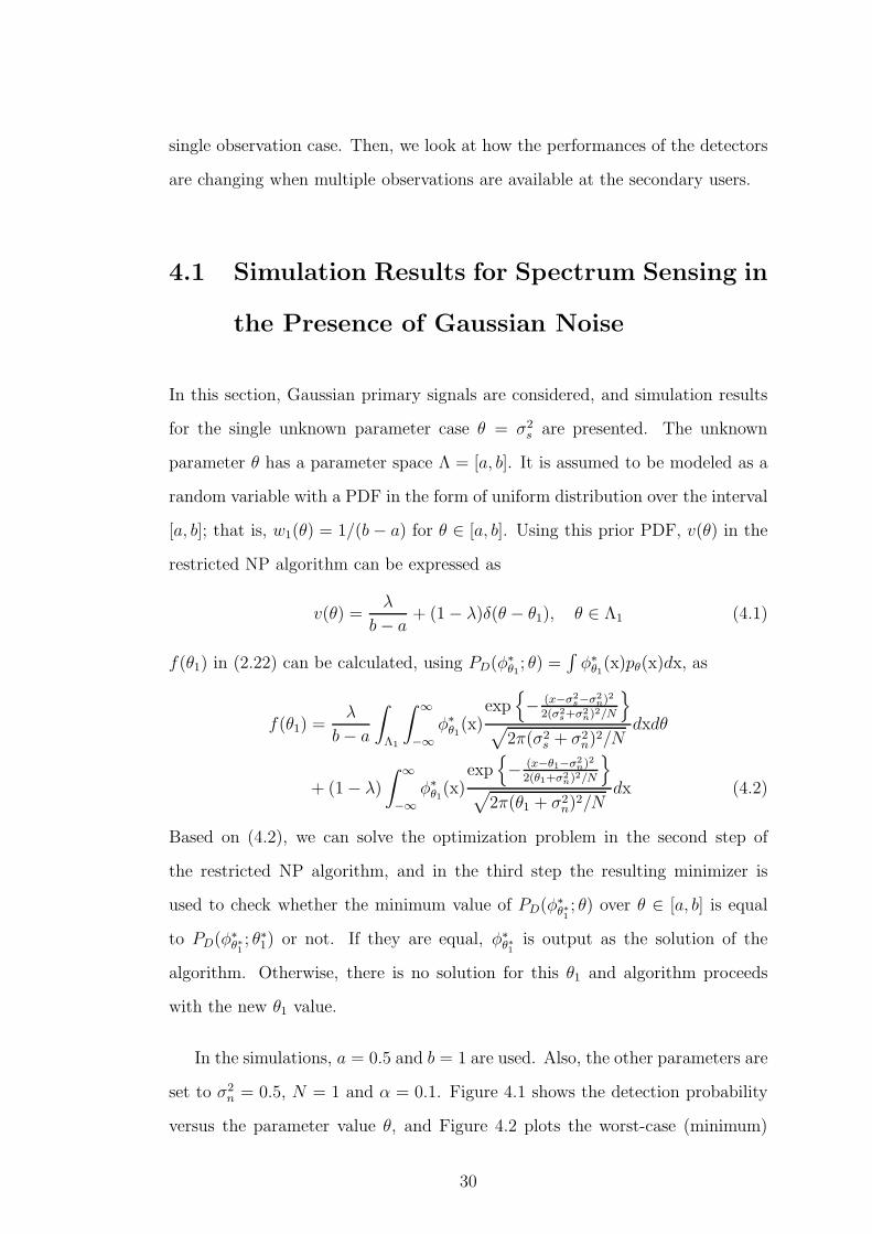
4.1 Simulation Results for Spectrum Sensing in

the Presence of Gaussian Noise

In this section, Gaussian primary signals are considered, and simulation results

for the single unknown parameter case θ = σ2s are presented. The unknown

parameter θ has a parameter space Λ = [a, b]. It is assumed to be modeled as a

random variable with a PDF in the form of uniform distribution over the interval

[a, b]; that is, w1(θ) = 1/(b− a) for θ ∈ [a, b]. Using this prior PDF, v(θ) in the

restricted NP algorithm can be expressed as

v(θ) =λ

b− a+ (1− λ)δ(θ − θ1), θ ∈ Λ1 (4.1)

f(θ1) in (2.22) can be calculated, using PD(φ∗θ1; θ) =

∫φ∗θ1(x)pθ(x)dx, as

f(θ1) =λ

b− a

∫

Λ1

∫ ∞

−∞φ∗θ1(x)

exp{− (x−σ2

s−σ2n)

2

2(σ2s+σ2

n)2/N

}

√2π(σ2

s + σ2n)

2/Ndxdθ

+ (1− λ)

∫ ∞

−∞φ∗θ1(x)

exp{− (x−θ1−σ2

n)2

2(θ1+σ2n)

2/N

}

√2π(θ1 + σ2

n)2/N

dx (4.2)

Based on (4.2), we can solve the optimization problem in the second step of

the restricted NP algorithm, and in the third step the resulting minimizer is

used to check whether the minimum value of PD(φ∗θ∗1; θ) over θ ∈ [a, b] is equal

to PD(φ∗θ∗1; θ∗1) or not. If they are equal, φ∗

θ∗1is output as the solution of the

algorithm. Otherwise, there is no solution for this θ1 and algorithm proceeds

with the new θ1 value.

In the simulations, a = 0.5 and b = 1 are used. Also, the other parameters are

set to σ2n = 0.5, N = 1 and α = 0.1. Figure 4.1 shows the detection probability

versus the parameter value θ, and Figure 4.2 plots the worst-case (minimum)

30

0.5 0.6 0.7 0.8 0.9 10.4

0.45

0.5

0.55

0.6

0.65

0.7

0.75

θ

Det

ectio

n P

roba

bilit

y

Restricted NPGLRTEnergy Detection

Figure 4.1: Detection probability versus θ for the three approaches for a = 0.5,b = 1, σ2

n = 0.5, N = 1 and α = 0.1.

and average detection probabilities versus λ for the three approaches. As can be

seen from Figure 4.2 the performance of the restricted NP approach stays the

same for all λ values in this scenario, so the results in Figure 4.1 are valid for all

the restricted NP solutions in this case. Both Figure 4.1 and Figure 4.2 shows

that the GLRT and the restricted NP approaches have the same performance

for all parameter values, and their performance are significantly much better

than the performance of the energy detection approach. From these results we

observe that the same decision rule is obtained for all values of λ for this problem.

That is, changing λ value does not change the performance of the restricted NP

approach for this problem.

As another example, the previous scenario is considered for N = 5. Figure

4.3 indicates the probability of detection versus θ for this case and in Figure

4.4 the worst-case (minimum) and average detection probabilities versus λ are

plotted. In general, the same observations as in the previous example are made.

31

0 0.2 0.4 0.6 0.8 10.4

0.42

0.44

0.46

0.48

0.5

0.52

0.54

0.56

0.58

λ

Restricted NPGLRTEnergy Detection

Average Det. Prob.

Minimum Det. Prob.

Figure 4.2: Detection probability versus λ for the three approaches for a = 0.5,b = 1, σ2

n = 0.5, N = 1 and α = 0.1.

However, detection probabilities increase significantly due to the increase in the

number of samples. Also, differences between the performance of the energy

detection and other approaches decrease remarkably as the number of samples

increase. Actually, they almost have the same performance if we further increase

the number of samples (see Figure 4.5).

In addition to the one parameter case, simulations are performed also for the

generic two-parameter case where the parameters are [θ11 θ12] = [σ2s E {|s|4}].

As in the one parameter case, the prior distributions of parameters θ11 and θ12 are

assumed uniform over [a, b] and [c, d], respectively. In the simulations, a = b =

c = d = 0.5 are used; that is, the parameter set is defined as Λ1 = [0.5, 1]×[0.5, 1].

Also, the other parameters are set to σ2n = 0.5, N = 1, and α = 0.2. Figure 4.6

shows the detection probabilities versus the parameters for the restricted NP,

GLRT, and energy detection approaches. Similar to the one parameter case, the

restricted NP and the GLRT techniques achieve a larger average and minimum

32

0.5 0.6 0.7 0.8 0.9 10.65

0.7

0.75

0.8

0.85

0.9

θ

Det

ectio

n P

roba

bilit

y

Restricted NPGLRTEnergy Detection

Figure 4.3: Detection probability versus θ for the three approaches for a = 0.5,b = 1, σ2

n = 0.5, N = 5 and α = 0.1.

0 0.2 0.4 0.6 0.8 1

0.68

0.7

0.72

0.74

0.76

0.78

0.8

λ

Restricted NPGLRTEnergy Detection

Average Det. Prob.

Minimum Det. Prob.

Figure 4.4: Detection probability versus λ for the three approaches for a = 0.5,b = 1, σ2

n = 0.5, N = 5 and α = 0.1.

33

0.5 0.6 0.7 0.8 0.9 10.82

0.84

0.86

0.88

0.9

0.92

0.94

0.96

θ

Det

ectio

n P

roba

bilit

y

Restricted NPGLRTEnergy Detection

Figure 4.5: Detection probability versus θ for the three approaches for a = 0.5,b = 1, σ2

n = 0.5, N = 10 and α = 0.1.

detection probabilities than the energy detection approach and they perform

almost similarly at all parameter values.

In conclusion, for the spectrum sensing problem specified in (3.5), the re-

stricted NP approach does not provide any significant improvements over the

existing GLRT approach. Hence, we should consider different scenarios in which

the restricted NP approach can provide unique advantages. This is performed in

the next section.

34

0.50.6

0.70.8

0.91

0.50.6

0.70.8

0.9

0.4

0.45

0.5

0.55

0.6

0.65

0.7

θ11

θ12

Det

ectio

n P

roba

bilit

y Rest. NP &GLRT

Energy Detection

Figure 4.6: Detection probability versus θ11 and θ12 for the three approaches forσ2n = 0.5, N = 1 and α = 0.2. The restricted NP and the GLRT approaches

have almost the same performance, while the energy detection results in lowerdetection probability for most parameter values.

4.2 Simulation Results for Spectrum Sensing

over Non-Gaussian Channels

4.2.1 Single Observation Case

In this section, we consider the Gaussian mixture noise models and present sim-

ulation results for this scenario. For the problem formulation (3.16) in Chapter

3, θ is modeled as a random variable with a PDF in the form of uniform distri-

bution over the interval [a, b]; that is, the parameter set under H1 is Λ1 = [a, b].

Since noise has Gaussian mixture distribution, the conditional PDF of X for a

given value of θ can be expressed as

pθ(x) =

Nm∑

i=1

νi√2π

exp

(−(x− θ − µi)

2

2ǫ2i

)(4.3)

35

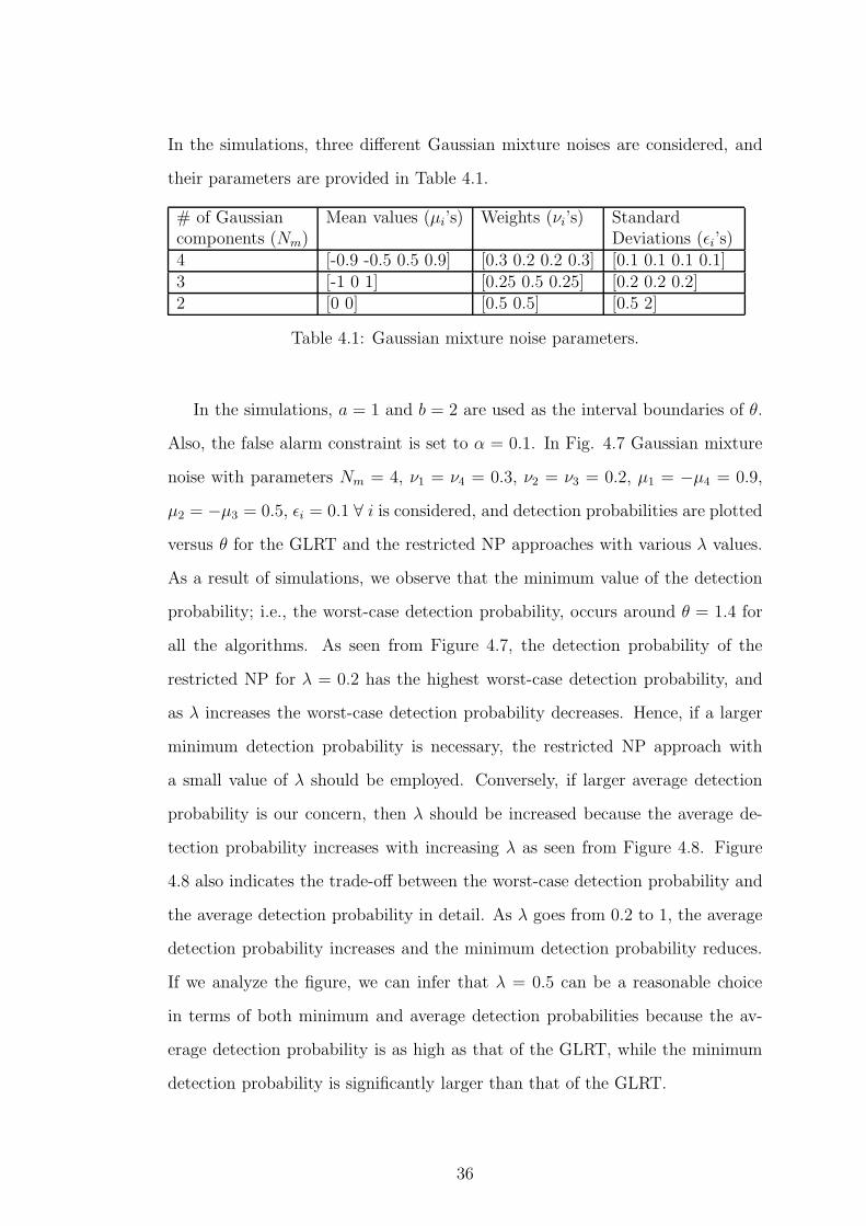
In the simulations, three different Gaussian mixture noises are considered, and

their parameters are provided in Table 4.1.

# of Gaussiancomponents (Nm)

Mean values (µi’s) Weights (νi’s) StandardDeviations (ǫi’s)

4 [-0.9 -0.5 0.5 0.9] [0.3 0.2 0.2 0.3] [0.1 0.1 0.1 0.1]3 [-1 0 1] [0.25 0.5 0.25] [0.2 0.2 0.2]2 [0 0] [0.5 0.5] [0.5 2]

Table 4.1: Gaussian mixture noise parameters.

In the simulations, a = 1 and b = 2 are used as the interval boundaries of θ.

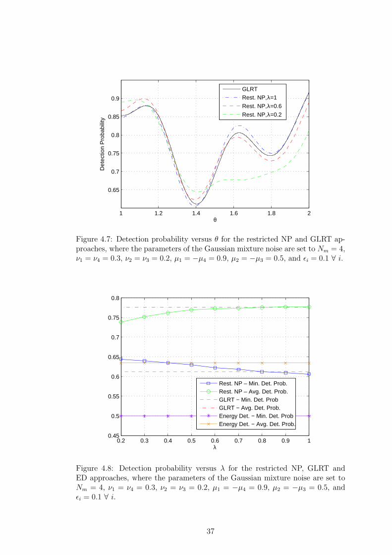
Also, the false alarm constraint is set to α = 0.1. In Fig. 4.7 Gaussian mixture

noise with parameters Nm = 4, ν1 = ν4 = 0.3, ν2 = ν3 = 0.2, µ1 = −µ4 = 0.9,

µ2 = −µ3 = 0.5, ǫi = 0.1 ∀ i is considered, and detection probabilities are plotted

versus θ for the GLRT and the restricted NP approaches with various λ values.

As a result of simulations, we observe that the minimum value of the detection

probability; i.e., the worst-case detection probability, occurs around θ = 1.4 for

all the algorithms. As seen from Figure 4.7, the detection probability of the

restricted NP for λ = 0.2 has the highest worst-case detection probability, and

as λ increases the worst-case detection probability decreases. Hence, if a larger

minimum detection probability is necessary, the restricted NP approach with

a small value of λ should be employed. Conversely, if larger average detection

probability is our concern, then λ should be increased because the average de-

tection probability increases with increasing λ as seen from Figure 4.8. Figure

4.8 also indicates the trade-off between the worst-case detection probability and

the average detection probability in detail. As λ goes from 0.2 to 1, the average

detection probability increases and the minimum detection probability reduces.

If we analyze the figure, we can infer that λ = 0.5 can be a reasonable choice

in terms of both minimum and average detection probabilities because the av-

erage detection probability is as high as that of the GLRT, while the minimum

detection probability is significantly larger than that of the GLRT.

36

1 1.2 1.4 1.6 1.8 2

0.65

0.7

0.75

0.8

0.85

0.9

θ

Det

ectio

n P

roba

bilit

y

GLRT

Rest. NP, λ=1

Rest. NP, λ=0.6

Rest. NP, λ=0.2

Figure 4.7: Detection probability versus θ for the restricted NP and GLRT ap-proaches, where the parameters of the Gaussian mixture noise are set to Nm = 4,ν1 = ν4 = 0.3, ν2 = ν3 = 0.2, µ1 = −µ4 = 0.9, µ2 = −µ3 = 0.5, and ǫi = 0.1 ∀ i.

0.2 0.3 0.4 0.5 0.6 0.7 0.8 0.9 10.45

0.5

0.55

0.6

0.65

0.7

0.75

0.8

λ

Rest. NP – Min. Det. Prob.Rest. NP – Avg. Det. Prob.GLRT − Min. Det. ProbGLRT − Avg. Det. Prob.Energy Det. − Min. Det. ProbEnergy Det. − Avg. Det. Prob.

Figure 4.8: Detection probability versus λ for the restricted NP, GLRT andED approaches, where the parameters of the Gaussian mixture noise are set toNm = 4, ν1 = ν4 = 0.3, ν2 = ν3 = 0.2, µ1 = −µ4 = 0.9, µ2 = −µ3 = 0.5, andǫi = 0.1 ∀ i.

37

1 1.2 1.4 1.6 1.8 20.4

0.45

0.5

0.55

0.6

0.65

0.7

0.75

0.8

0.85

0.9

θ

Det

ectio

n P

roba

bilit

y

GLRT

Rest. NP, λ=1

Rest. NP, λ=0.5

Rest. NP, λ=0.1

Rest. NP, λ=0

Figure 4.9: Detection probability versus θ for the restricted NP and GLRT ap-proaches, where the parameters of the Gaussian mixture noise are set to Nm = 3,ν1 = ν3 = 0.25, ν2 = 0.5, µ1 = −µ3 = 1, µ2 = 0, and ǫi = 0.2 ∀ i.

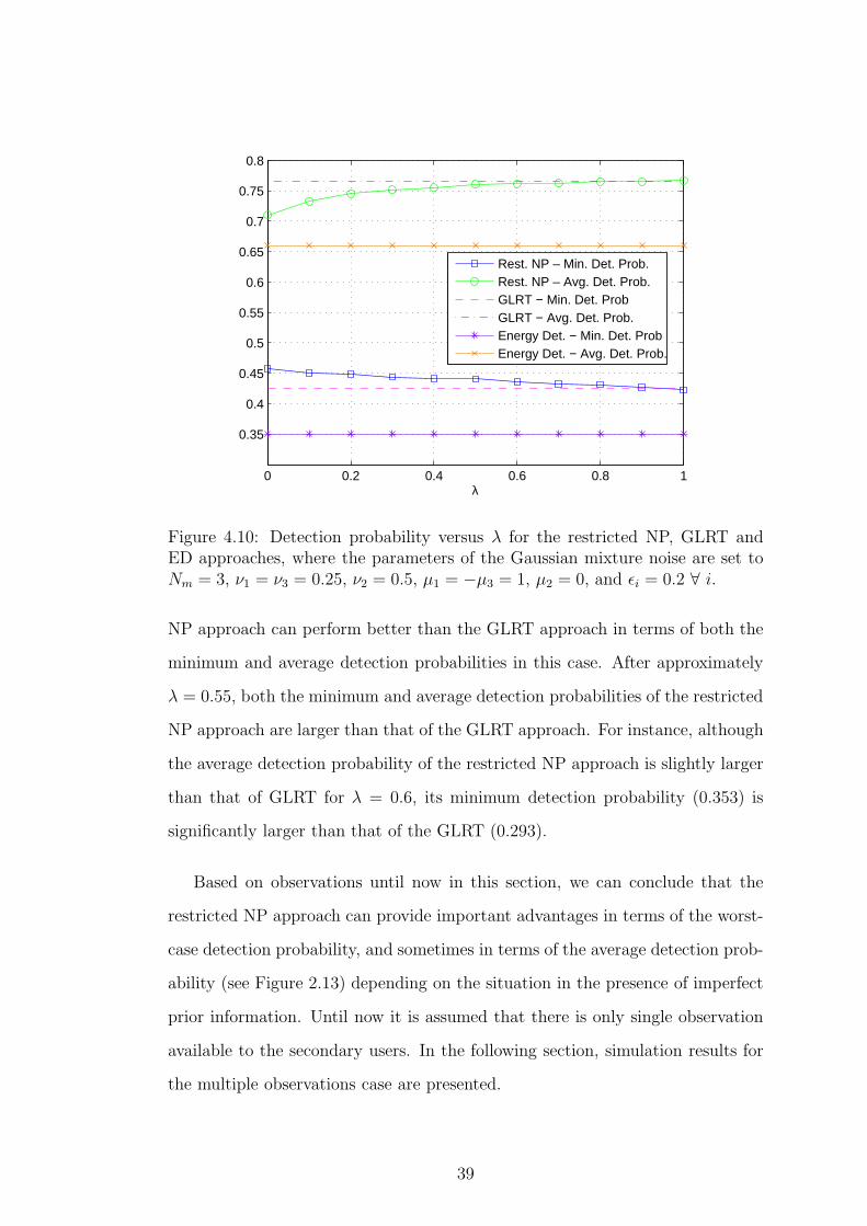
For the second Gaussian mixture noise parameter set, which is Nm = 3, ν1 =

ν3 = 0.25, ν2 = 0.5, µ1 = −µ3 = 1, µ2 = 0, and ǫi = 0.2 ∀ i, simulation results

for detection probability versus θ and λ are presented in Figure 4.9 and Figure

4.10, respectively. Similar tradeoffs as in the previous scenario are observed. The

importance of this scenario is that this kind of mixture noise can be encountered

in practice. For example, it can correspond to the sum of zero-mean Gaussian

noise and interference which is due to two users that result in signal values of

±0.5 with equal probabilities at the receiver.

In the third simulations, the parameters of the Gaussian mixture noise are

set to Nm = 2, ν1 = ν2 = 0.5, µ1 = µ2 = 0, ǫ1 = 0.5, and ǫ2 = 2. The noise

model employed in this scenario is practically important. The mixture of zero-

mean Gaussian random variables with different variances is often used to model

man-made noise, impulsive phenomena, and certain sorts of ultra-wideband inter-

ference [45]. Figure 4.11 and Figure 4.12 shows the detection probability versus θ

and λ for this scenario, respectively. Unlike the previous two cases, the restricted

38

0 0.2 0.4 0.6 0.8 1

0.35

0.4

0.45

0.5

0.55

0.6

0.65

0.7

0.75

0.8

λ

Rest. NP – Min. Det. Prob.Rest. NP – Avg. Det. Prob.GLRT − Min. Det. ProbGLRT − Avg. Det. Prob.Energy Det. − Min. Det. ProbEnergy Det. − Avg. Det. Prob.

Figure 4.10: Detection probability versus λ for the restricted NP, GLRT andED approaches, where the parameters of the Gaussian mixture noise are set toNm = 3, ν1 = ν3 = 0.25, ν2 = 0.5, µ1 = −µ3 = 1, µ2 = 0, and ǫi = 0.2 ∀ i.

NP approach can perform better than the GLRT approach in terms of both the

minimum and average detection probabilities in this case. After approximately

λ = 0.55, both the minimum and average detection probabilities of the restricted

NP approach are larger than that of the GLRT approach. For instance, although

the average detection probability of the restricted NP approach is slightly larger

than that of GLRT for λ = 0.6, its minimum detection probability (0.353) is

significantly larger than that of the GLRT (0.293).

Based on observations until now in this section, we can conclude that the

restricted NP approach can provide important advantages in terms of the worst-

case detection probability, and sometimes in terms of the average detection prob-

ability (see Figure 2.13) depending on the situation in the presence of imperfect

prior information. Until now it is assumed that there is only single observation

available to the secondary users. In the following section, simulation results for

the multiple observations case are presented.

39

1 1.2 1.4 1.6 1.8 20.25

0.3

0.35

0.4

0.45

0.5

0.55

0.6

0.65

θ

Det

ectio

n P

roba

bilit

y

GLRT

Rest. NP, λ=1

Rest. NP, λ=0.5

Rest. NP, λ=0.1

Rest. NP, λ=0

Figure 4.11: Detection probability versus θ for the restricted NP and GLRTapproaches, where the parameters of the Gaussian mixture noise are set to Nm =2, ν1 = ν2 = 0.5, µ1 = µ2 = 0, ǫ1 = 0.5, and ǫ2 = 2.

0.2 0.3 0.4 0.5 0.6 0.7 0.8 0.9 10.1

0.15

0.2

0.25

0.3

0.35

0.4

0.45

0.5

0.55

λ

Rest. NP – Min. Det. Prob.Rest. NP – Avg. Det. Prob.GLRT − Min. Det. ProbGLRT − Avg. Det. Prob.Energy Det. − Min. Det. ProbEnergy Det. − Avg. Det. Prob.

Figure 4.12: Detection probability versus λ for the restricted NP, GLRT andED approaches, where the parameters of the Gaussian mixture noise are set toNm = 2, ν1 = ν2 = 0.5, µ1 = µ2 = 0, ǫ1 = 0.5, and ǫ2 = 2.

40

1 1.2 1.4 1.6 1.8 2

0.82

0.84

0.86

0.88

0.9

0.92

0.94

0.96

0.98

1

θ

Det

ectio

n P

roba

bilit

y

Energy DetectorGLRTRest. NP, λ=0Rest. NP, λ=0.5Rest. NP, λ=1

Figure 4.13: Detection probability versus θ for the restricted NP, GLRT, andenergy detection approaches for M = 5.

4.2.2 Multiple Observations Case

For the simulations of the multiple observations case, the same distribution for θ

and the same value for α are used. Also, the Gaussian mixture noise parameters

are set to Nm = 3, ν1 = ν3 = 0.25, ν2 = 0.5, µ1 = −µ3 = 1, µ2 = 0, and ǫi = 0.2.

First, in Figure 4.13 detection probability versus θ is plotted for all approaches

when M = 5 observations are made. It is observed that the GLRT and the

restricted NP approaches perform much better than the energy detection. Also,

the restricted NP approach provides some improvements over GLRT in terms

of minimum detection and average detection performance for various λ values.

This can be seen more clearly from Figure 4.14, in which the minimum and

average detection probabilities are plotted versus λ. A good tradeoff between

the minimum and average detection probabilities can be obtained by employing

the restricted NP approach.

41

0 0.2 0.4 0.6 0.8 10.95

0.955

0.96

0.965

0.97

0.975

0.98

0.985

0.99

0.995

1

λ

Rest. NP – Min. Det. Prob.Rest. NP – Avg. Det. Prob.GLRT − Min. Det. ProbGLRT − Avg. Det. Prob.Energy Det. − Min. Det. Prob Energy Det. − Avg. Det. Prob.

Figure 4.14: Detection probability versus λ for the restricted NP, GLRT, andenergy detection approaches for M = 5. For the energy detector, the minimumdetection probability is 0.808, which is not shown in the figure.

The performance of the energy detector and GLRT is also investigated for

various numbers of observations. Figure 4.15 and 4.16 show that the perfor-

mance of both GLRT and energy detector improves with the increasing number

of observations. Also, GLRT performs significantly better than energy detector

for the same number of observations. Since the restricted NP approach performs

similarly to GLRT with improved minimum detection or average detection prob-

ability depending on the value of λ, we can infer that Figure 4.15 also provides

information about the performance of the restricted NP approach.

42

1 1.2 1.4 1.6 1.8 20.7

0.75

0.8

0.85

0.9

0.95

1

θ

Det

ectio

n P

roba

bilit

y

M=2M=5M=10

Figure 4.15: Detection probability versus θ for the GLRT approach for variousnumbers of observations.

1 1.2 1.4 1.6 1.8 20.5

0.55

0.6

0.65

0.7

0.75

0.8

0.85

0.9

0.95

1

θ

Det

ectio

n P

roba

bilit

y

M=2M=5M=10M=20

Figure 4.16: Detection probability versus θ for the energy detection approach forvarious numbers of observations.

43

Chapter 5

CONCLUSIONS

In this thesis, we have studied the spectrum sensing problem for cognitive radio

systems in the presence of uncertainty in the prior distribution of primary users’

signal. In Chapter 1, we have first provided background information about cog-

nitive radio and the spectrum sensing problem in cognitive radio systems. Then,

the general spectrum sensing problem has been formulated. In addition, three

popular spectrum sensing methods; namely, energy detection, matched filtering,

and cyclostationary detection have been explained.

In Chapter 2, background information about common hypothesis testing tech-

niques has been provided. We have emphasized the necessity for techniques

which take partial information into account. Therefore, we have presented the

restricted NP approach [27], an application of the restricted Bayes approach to

the NP framework. The problem formulation for the restricted NP approach

has been provided, and the algorithm for obtaining the optimal decision rule has

been presented.

In Chapter 3, we have investigated how the restricted NP approach can be em-

ployed to solve spectrum sensing problem in cognitive radio. We know that some

information about the prior distribution of primary users’ signal is available in

44

many cases, but that information is not perfect most of the time. This makes the

restricted NP approach well suited for our problem. First, we consider Gaussian

noise for both Gaussian primary signals and for any kind of primary signals. The

simulations in Chapter 4 have shown that although the restricted NP approach

outperforms energy detection, it does not provide any significant improvements

over the existing GLRT approach. This forced us to consider different scenarios,

hence we have studied non-Gaussian noise for the same problem. Particularly,

Gaussian mixture noise has been considered, and the simulation results have

been presented in Chapter 4. The results have shown that the restricted NP

approach performed better than GLRT in terms of the minimum detection prob-

ability for different uncertainty levels. Also, in some scenarios (e.g., see Fig. 4.11

and 4.12) the restricted NP approach has higher average detection probability

than GLRT after a certain λ value and still it has significantly larger minimum

detection probability than GLRT for all λ values. Additionally, we have per-

formed simulations for the case of multiple observations. The simulation results

have shown us that performance of GLRT improves with the increasing number

of observations which means the performance of the restricted NP also improves

because it exhibits similar trends to GLRT with improved minimum detection

and/or average detection probability depending on the value of λ.

As a future work, cooperation among cognitive radios which use the restricted

NP approach as spectrum sensing method can be employed to compensate the

effects of shadowing and multipath fading, and as a result to obtain improved

sensing performance.

45

APPENDIX A

Calculation of Mean and

Variance of X

Under hypothesis H1, mean of X = 1N

∑Ni=1 |xi|2 can be found as follows:

E {X} =1

NE

{N∑

i=1

|xi|2}

=1

N

N∑

i=1

E{|si + ni|2

}

=1

N

N∑

i=1

E

{|si|2

}︸ ︷︷ ︸

σ2s

+E {sin∗i }︸ ︷︷ ︸

0

+E {nis∗i }︸ ︷︷ ︸

0

+E{|ni|2

}︸ ︷︷ ︸

σ2n

= σ2s + σ2

n. (A.1)

Since PS users are absent under hypothesis H0, E {X} is equal to σ2n under

H0.

46

Under hypothesis H1, V ar(X) can be obtained as follows:

V ar(X) = E{|X − E {X} |2

}

= E

{(1

N

N∑

i=1

|si + ni|2 − (σ2s + σ2

n))2

}

=1

NE{(|s|2 + |n|2 + sn∗ + s∗n− σ2

s − σ2n)

2}

=1

NE{|s|4 + 2|s|2|n|2 + |n|4 + (sn∗)2 + 2(sn∗)(s∗n) + (s∗n)2

}

+1

NE{2|s|2(sn∗ + s∗n) + 2|n|2(sn∗ + s∗n) + (σ2

s + σ2n)

2 − 2|s|2(σ2s + σ2

n)}

− 1

NE{2|n|2(σ2

s + σ2n) + 2sn∗(σ2

s + σ2n) + 2s∗n(σ2

s + σ2n)}

=1

NE{|s|4 + 4|s|2|n|2 + |n|4 + (σ2

s + σ2n)

2 − 2σ4s − 4σ2

sσ2n

}

=1

N(E

{|s|4

}+ 2σ2

sσ2n + σ4

n − σ4s)

=1

N(E

{|s|4

}+ 2σ4

n − (σ2s − σ2

n)2) (A.2)

Since both si and ni have circularly symmetric distribution with zero-mean, we

have E {s2} = E {(s∗)2} = 0 and E{n2} = E {(n∗)2} = 0. Also, E {|n|4} = 2σ4n

due to the Gaussian distribution assumption. In short, using circular symmetric-

ity, zero mean, independency of s and n, and the Gaussian n assumptions we

obtain V ar(X). Similar to the mean, the variance of X is equal to σ4n/N under

hypothesis H0 because no PS users are present under H0.

47

Bibliography

[1] NTIA, “U.S. frequency allocations.” http://www.ntia.doc.gov/osmhome/

allochrt.pdf.

[2] D. Cabric, Cognitive Radios: System Design Perspective. PhD thesis, Uni-

versity of California at Berkeley, 2006.

[3] I. F. Akyildiz, W. Y. Lee, M. C. Vuran, and S. Mohanty, “Next genera-

tion/dynamic spectrum access/cognitive radio wireless networks: A survey,”

Computer Networks (ELSEVIER), vol. 50, pp. 2127–2159, 2006.

[4] H. Wang, G. Noh, D. Kim, S. Kim, , and D. Hong, “Advanced sensing tech-

niques of energy detection in cognitive radios,” Journal of Communications

and Networks, vol. 12, no. 1, pp. 19–29, February 2010.

[5] FCC, “Connecting America: The national broadband plan.”

http://http://www.broadband.gov/plan/5-spectrum/.

[6] FCC, “Spectrum policy task force report,” Proceedings of the Federal Com-

munications Commission (FCC’02), Washington, DC, USA, November

2002.

[7] J. Mitola and G. Q. Maguire, “Cognitive radio: Making software radios

more personal,” IEEE Personal Communications, vol. 6, no. 4, pp. 13–18,

August 1999.

48

[8] Y. Zeng, Y. C. Liang, A. T. Hoang, and R. Zhang, “A review on spectrum

sensing for cognitive radio: Challenges and solutions,” EURASIP Journal

on Advances in Signal Processing, pp. 1–16, 2010.

[9] L. Shen, H. Wang, W. Zhang, and Z. Zhao, “Blind spectrum sensing for cog-

nitive radio channels with noise uncertainty,” IEEE Transactions on Wire-

less Communications, vol. 10, no. 6, pp. 1721–1724, June 2011.

[10] R. Lopez-Valcarce, G. Vazquez-Vilar, and J. Sala, “Multiantenna spectrum

sensing for cognitive radio: Overcoming noise uncertainty,” in 2nd Interna-

tional Workshop on Cognitive Information Processing, pp. 310–315, 14-16

June, 2010.

[11] G. Ji and H. Zhu, “Noise uncertainty study of the low SNR energy detector

in cognitive radio,” in in Proc. AICI (1), pp. 248–255, 2010.

[12] S. M. Kay, Fundamentals of Statistical Signal Processing: Detection Theory.

Prentice Hall, Upper Saddle River, NJ, USA, 1998.

[13] A. Sahai and D. Cabric, “Spectrum sensing: Fundamental limits and prac-

tical challenges,” in IEEE International Symposium on New Frontiers in

Dynamic Spectrum Access Networks (DySPAN’05), November, 2005.

[14] W. A. Gardner, “Exploitation of spectral redundancy in cyclostationary

signals,” IEEE Signal Processing Magazine, vol. 8, no. 2, pp. 14–36, April,

1991.

[15] W. A. Gardner, “Spectral correlation of modulated signals: Part I-analog

modulation,” IEEE Transactions on Communications, vol. 35, no. 6,

pp. 584–594, 1987.

[16] W. A. Gardner, “Spectral correlation of modulated signals: Part II-

digital modulation,” IEEE Transactions on Communications, vol. 35, no. 6,

pp. 595–601, 1987.

49

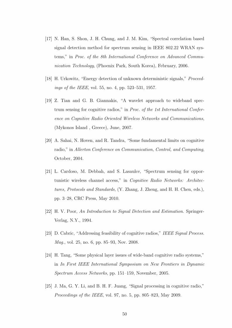
[17] N. Han, S. Shon, J. H. Chung, and J. M. Kim, “Spectral correlation based

signal detection method for spectrum sensing in IEEE 802.22 WRAN sys-

tems,” in Proc. of the 8th International Conference on Advanced Commu-

nication Technology, (Phoenix Park, South Korea), February, 2006.

[18] H. Urkowitz, “Energy detection of unknown deterministic signals,” Proceed-

ings of the IEEE, vol. 55, no. 4, pp. 523–531, 1957.

[19] Z. Tian and G. B. Giannakis, “A wavelet approach to wideband spec-

trum sensing for cognitive radios,” in Proc. of the 1st International Confer-

ence on Cognitive Radio Oriented Wireless Networks and Communications,

(Mykonos Island , Greece), June, 2007.

[20] A. Sahai, N. Hoven, and R. Tandra, “Some fundamental limits on cognitive

radio,” in Allerton Conference on Communication, Control, and Computing,

October, 2004.

[21] L. Cardoso, M. Debbah, and S. Lasaulce, “Spectrum sensing for oppor-

tunistic wireless channel access,” in Cognitive Radio Networks: Architec-

tures, Protocols and Standards, (Y. Zhang, J. Zheng, and H. H. Chen, eds.),

pp. 3–28, CRC Press, May 2010.

[22] H. V. Poor, An Introduction to Signal Detection and Estimation. Springer-

Verlag, N.Y., 1994.

[23] D. Cabric, “Addressing feasibility of cognitive radios,” IEEE Signal Process.

Mag., vol. 25, no. 6, pp. 85–93, Nov. 2008.

[24] H. Tang, “Some physical layer issues of wide-band cognitive radio systems,”

in In First IEEE International Symposium on New Frontiers in Dynamic

Spectrum Access Networks, pp. 151–159, November, 2005.

[25] J. Ma, G. Y. Li, and B. H. F. Juang, “Signal processing in cognitive radio,”

Proceedings of the IEEE, vol. 97, no. 5, pp. 805–823, May 2009.

50

[26] G. Ganesan and Y. Li, “Cooperative spectrum sensing in cognitive radio

networks,” in First IEEE International Symposium on New Frontiers in

Dynamic Spectrum Access Networks, pp. 137–143, November, 2005.

[27] S. Bayram and S. Gezici, “On the restricted Neyman-Pearson approach for

composite hypothesis-testing in the presence of prior distribution uncer-

tainty,” IEEE Trans. Sig. Processing, vol. 59, no. 10, pp. 5056–5065, 2011.

[28] J. Zhang, “Multiple hypotheses testing with partial prior information,” Sta-

tistica Sinica, vol. 9, pp. 1131–1140, 1999.

[29] J. R. Blum and J. Rosenblatt, “On partial a priori information in statistical

inference,” The Annals of Mathematical Statistics, vol. 38, no. 6, pp. 1671–

1678, Dec., 1967.

[30] J. L. Hodges and E. L. Lehmann, “The use of previous experience in reaching

statistical decisions,” The Annals of Mathematical Statistics, vol. 23, no. 3,

pp. 396–407, Sep. 1952.

[31] H. Robbins, “The empirical Bayes approach to statistical decision prob-

lems,” The Annals of Mathematical Statistics, vol. 35, no. 1, pp. 1–20, 1964.

[32] L. J. Savage, The Foundations of Statistics, 2nd ed. Dover, N.Y., 1972.

[33] H. Kudo, “On partial prior information and the property of parametric suf-

ficiency,” Fifth Berkeley Symposium on Mathematical Statistics and Proba-

bility, vol. 1, pp. 251–265, 1967.

[34] E. L. Lehmann and J. P. Romano, Testing Statistical Hypotheses, 3rd ed.

Springer, N.Y., 2005.

[35] J. Cvitanic and I. Karatzas, “Generalized Neyman-Pearson lemma via con-

vex duality,” Bernoulli, vol. 7, no. 1, pp. 79–97, 2001.

[36] B. Rudloff and I. Karatzas, “Testing composite hypotheses via convex du-

ality,” Bernoulli, vol. 16, no. 4, pp. 1224–1239, 2010.

51

[37] E. L. Lehmann, “Some history of optimality,” Lecture Notes-Monograph

Series, vol. 57, pp. 11–17, 2009.

[38] N. Begum and M. L. King, “A new class of test for testing a composite null

against a composite alternative hypothesis,” in Proc. Australasian Meeting

of the Econometric Society, 2007.

[39] J. O. Berger, B. Boukai, and Y. Wang, “Unified frequentist and Bayesian

testing of a precise hypothesis,” Statistical Science, vol. 12, no. 3, pp. 133–

160, 1997.

[40] M. C. Gursoy and S. Gezici, “On the interplay between channel sensing and

estimation in cognitive radio systems,” in Proc. IEEE Global Telecommuni-

cations Conference (GLOBECOM), (Houston, Texas), 5-9 Dec. 2011.

[41] T. J. Lim, R. Zhang, Y. C. Liang, and Y. Zeng, “GLRT-based spectrum

sensing for cognitive radio,” Proc. IEEE Global Telecommunications Con-

ference (GLOBECOM), New Orleans, LA, Nov. 30-Dec. 4 2008.

[42] T. Wimalajeewa and P. K. Varshney, “A non-parametric approach for spec-

trum sensing with multiple antenna cognitive radios in the presence of non-

gaussian noise,” in IEEE Wireless Communications and Networking Con-

ference (WCNC), (Cancun, Quintana Roo), March, 2011.

[43] F. Moghimi, A. Nasri, , and R. Schober, “lp-norm spectrum sensing for

cognitive radio networks impaired by non-Gaussian noise,” in IEEE Global

Telecommunications Conference (GLOBECOM), (Honolulu, HI), December,

2009.

[44] S. J. Zahabi and A. A. Tadaion, “Local spectrum sensing in non-Gaussian

noise,” in IEEE 17th International Conference on Telecommunications

(ICT), (Doha), April, 2010.

52

[45] F. Moghimi, A. Nasri, , and R. Schober, “Adaptive lp-norm spectrum sens-

ing for cognitive radio networks,” IEEE Transactions on Communications,

vol. 59, no. 7, p. 19341945, July 2011.

53