NISTIR 6964

Results from Simulation and Laboratory

Testing of Air Handling Unit and Variable Air Volume Box Diagnostic Tools

Natascha S. Castro Jeffrey Schein

Cheol Park Michael A. Galler Steven T. Bushby

U.S. DEPARTMENT OF COMMERCE

National Institute of Standards and Technology Building Environment Division

Building and Fire Research Laboratory Gaithersburg, MD 20899-8631

John M. House

Iowa Energy Center Ames, IA

NISTIR 6964

Results from Simulation and Laboratory Testing of Air Handling Unit and Variable

Air Volume Box Diagnostic Tools

Natascha S. Castro Jeffrey Schein

Cheol Park Michael A.Galler Steven T. Bushby

U.S. DEPARTMENT OF COMMERCE

National Institute of Standards and Technology Building Environment Division

Building and Fire Research Laboratory Gaithersburg, MD 20899-8631

John M. House

Iowa Energy Center Ames, IA

Prepared for:

Architectural Energy Corporation Boulder, Colorado

January 2003

U.S. Department of Commerce

Donald L. Evans, Secretary Technology Administration

Phillip J. Bond, Under Secretary for Technology National Institute of Standards and Technology

Arden L. Bement, Jr., Director

Abstract Control of building systems is becoming increasingly more intelligent and complex. This development both necessitates the use of automated diagnostics to ensure fault-free operation and enables diagnostic capabilities for the various building systems by providing a distributed platform that is powerful and flexible enough to perform fault detection and diagnostic (FDD). Most of today’s emerging FDD tools are stand-alone software products that do not reside in a building control system. Thus, trend data files must be processed off-line, or an interface to the building control system must be developed to enable on-line analysis. This is a cumbersome process and it does not scale well because all of the data must be obtained at a single point. A better approach would be to develop algorithms that can be embedded in commercial controllers so that the fault detection can be done as close to the source of the fault as possible. Only the result of the analysis needs to be conveyed to an operator or supervisory controller. AHU Performance Assessment Rules (APAR) is a diagnostic tool that uses a set of expert rules derived from mass and energy balances to detect common faults in air-handling units. Control signals are used to determine the mode of operation for the AHU. A subset of the expert rules corresponding to that mode of operation is then evaluated to determine if there is a mechanical fault or a control problem. VAV box Performance Assessment Control Charts (VPACC) is a diagnostic tool that uses a statistical quality control measures to detect faults or control problems in VAV boxes. This report describes the results of a research study to determine the effectiveness of these tools in detecting commonly found mechanical faults and control problems. The research involved a complementary set of laboratory experiments using commercial AHU and VAV box controllers under both normal operating conditions and operation with known faults, computer simulations, and emulations using the NIST Virtual Cybernetic Building Testbed (VCBT). The APAR and VPACC tools were both found to be successful at finding a wide variety of faults. It was also found that some faults could not be detected under certain operating conditions because the control system was able to mask the problem or because sensor data needed to detect the fault is not commonly available in commercial systems. Both tools appear to be suitable for embedding in commercial control products. Key words: BACnet, building automation and control, direct digital control, energy management systems, fault detection and diagnostics, cybernetic building systems

Acknowledgments This work was supported in part by the California Energy Commission Public Interest Energy Research (PIER) Program. The authors wish to acknowledge the assistance of Peter G. Loutzenhiser from Iowa State University and Daniela Marquez from University of Michigan who helped collect and process some of the data used in this report.

Table of Contents

1 Introduction............................................................................................................................. 1 2 Validation of Fault Models ..................................................................................................... 2

2.1 Air Handling Unit Faults ................................................................................................ 3 2.1.1 Supply Air Temperature Sensor Offset................................................................... 3 2.1.2 Stuck Open Recirculating Air Damper ................................................................... 8 2.1.3 Leaking Heating Coil Valve ................................................................................. 10

2.2 Variable-Air-Volume Box Faults ................................................................................. 14 2.2.1 Stuck Open VAV Box Damper............................................................................. 14 2.2.2 Stuck Open VAV Box Reheat Valve.................................................................... 19

2.3 Conclusions................................................................................................................... 21 3 FDD for Air Handling Units ................................................................................................. 21

3.1 System Description ....................................................................................................... 21 3.2 AHU Performance Assessment Rules (APAR) ............................................................ 23

3.2.1 Operational and Design Data Requirements......................................................... 26 3.2.2 Detecting and Diagnosing Faults .......................................................................... 27 3.2.3 Threshold Selection .............................................................................................. 27

3.3 Instrumentation Accuracy Requirements...................................................................... 28 3.4 Results from AHU Laboratory Experiments ................................................................ 28 3.5 Results from APAR Analysis of AHU Simulation Data Using HVACSIM+............... 33

3.5.1 Normal Operation ................................................................................................. 34 3.5.2 Simulated Faults.................................................................................................... 34

3.6 Results from AHU Emulation in the VCBT................................................................. 39 3.6.1 Faults Implemented............................................................................................... 40 3.6.2 Normal Operation ................................................................................................. 41 3.6.3 APAR Analysis & Results .................................................................................... 43

3.7 APAR User Interface .................................................................................................... 51 4 FDD for VAV ....................................................................................................................... 55

4.1 VAV box Performance Assessment Control Charts - VPACC .................................... 55 4.1.1 Control Charts....................................................................................................... 55 4.1.2 System Description ............................................................................................... 57 4.1.3 CUSUM Applied to VAV Box Diagnostics ......................................................... 58 4.1.4 Point requirements ................................................................................................ 59 4.1.5 Threshold Selection .............................................................................................. 60 4.1.6 Instrumentation Accuracy Requirements.............................................................. 60

4.2 Results from VAV Box Laboratory Experiments......................................................... 60 4.2.1 Faults Implemented............................................................................................... 60 4.2.2 Normal Operation ................................................................................................. 61 4.2.3 Control Charts....................................................................................................... 62

4.3 Results from VAV Box Simulation Using HVACSIM+............................................... 65 4.3.1 Faults Implemented............................................................................................... 66 4.3.2 Normal Operation ................................................................................................. 67 4.3.3 Control Charts....................................................................................................... 67

4.4 Results from VAV Box Emulation in the VCBT ......................................................... 71 4.4.1 Faults Implemented............................................................................................... 72

4.4.2 Normal Operation ................................................................................................. 73 4.4.3 Control Charts....................................................................................................... 73

5 Summary and Future Work................................................................................................... 83 6 References............................................................................................................................. 85 Attachment A: Nomenclature for Table 1 .................................................................................... 86

1 INTRODUCTION Control of building systems is becoming increasingly more intelligent and complex. The control infrastructure necessary for the operation of various building systems provides a distributed platform that is powerful and flexible enough to perform fault detection and diagnostics (FDD). Most of today’s emerging FDD tools are stand-alone software products that are not integrated with the building control system. Thus, trend data files must be processed off-line, or an interface to the building control system must be developed to enable on-line analysis. The purpose of the research effort described in this report is to develop, test, and demonstrate FDD methods that can detect common mechanical faults and control errors in air-handling units (AHUs) and variable-air-volume (VAV) boxes. The tools are intended to be sufficiently simple that they can be embedded in commercial building control systems and rely upon only sensor data and control signals that are commonly available in commercial building automation and control systems. AHU Performance Assessment Rules (APAR) is a diagnostic tool that uses a set of expert rules derived from mass and energy balances to detect common faults in air-handling units. Control signals are used to determine the mode of operation for the AHU. A subset of the expert rules corresponding to that mode of operation is then evaluated to determine if there is a mechanical fault or a control problem. VAV box Performance Assessment Control Charts (VPACC) is a diagnostic tool that uses a statistical quality control measures to detect faults or control problems in VAV boxes. VPACC can be applied to most VAV box control strategies. Fault thresholds are determined by statistical analysis of a database of “normal operation” data. This report describes the development and the results of a research study to determine the effectiveness of these tools in detecting commonly found mechanical faults and control problems. The FDD tools for AHUs and VAV boxes are being developed with distinct approaches because of the nature of the systems. VAV boxes are simple devices with a limited number of operation modes and possible faults. Because the building industry is sensitive to the first cost, the VAV boxes typically have little instrumentation and controllers with limited capability. However, VAV boxes are very numerous in a typical HVAC system, resulting in a large amount of data to be monitored for faults. AHUs are more complex and thus susceptible to more kinds of faults. They also tend to have more instrumentation and more capable controllers. The FDD tools for both systems are designed to be robust so that they can adapt to the variety of applications typical of their use. The research involved a complementary set laboratory of experiments using commercial AHU and VAV box controllers under both normal operating conditions and operation with known faults, emulations using the NIST Virtual Cybernetic Building Testbed (VCBT), and computer simulations using HVACSIM+. These three approaches compliment each other and provide a reasonable assurance that the results are representative of what can be expected in real building systems. The VCBT is a simulation-emulation environment that combines simulations of a building and its HVAC system with the emulation of the actual commercial controllers. It provides a way to

1

conduct tests under a wide variety of carefully controlled conditions and to compare the results of several different commercial products. Details of the VCBT design and operation are documented in NISTIR 6818, Using the Virtual Cybernetic Building Testbed and FDD Test Shell for FDD Tool Development [2]. Emulation provides a test environment that is closer to a real building because it uses real building controllers but, like simulation, it also provides carefully controlled and reproducible conditions. Because emulation is done in real time it takes much longer than simulation, making it more difficult to test a broad range of faults and conditions in a limited time. The emulation also provides a controlled testbed for verifying the capabilities of FDD tools that are used to interface with control systems in real buildings. It will also be used in the future as a platform for testing the FDD tools when they are embedded in commercial controllers. Simulation provides a way to expand the variety of weather and fault conditions without the real-time constraints of the experimental and emulation studies. The simulations were conducted using HVACSIM+[4]. The results from the laboratory experiments, emulations, and simulations were compared for a subset of test cases as a way to verify that the results are reasonable. The APAR and VPACC tools were both found to be successful at finding a wide variety of faults including stuck or leaking dampers and control valves, sensor drift, and improper control sequencing. It was also found that some faults could not be detected under certain operating conditions because the control system was able to mask the problem or because sensor data needed to detect the fault is not commonly available in commercial systems. Both tools appear to be suitable for embedding in commercial control products.

2 VALIDATION OF FAULT MODELS Numerous fault models for AHU and VAV box sensors and controlled devices have been implemented in HVACSIM+. Bushby et al. [2] provide detailed descriptions of the manner in which the faults were introduced in the simulation code. In this section, simulation data produced by three of the AHU faults and two of the VAV box faults implemented in HVACSIM+ and described by Bushby et al. [2] will be compared with data collected at the Iowa Energy Center Energy Resource Station (designated as the ERS throughout the remainder of this report) to ensure that the characteristics and trends observed in the simulation data are representative of real systems. The complete set of faults simulated is provided in Table 3.5 and includes sensor faults, stuck and leaking valve faults, and stuck and leaking damper faults for the AHU. The faults that are validated are a supply air temperature sensor offset fault, a stuck open recirculation air damper fault, and a leaking heating coil valve fault. The VAV box faults simulated are a stuck open or closed damper and a stuck open or closed reheat valve. The faults that are validated are a stuck open damper fault and a stuck open reheat valve fault. The set of faults that are validated is considered to be representative of the complete set since one fault of each type (sensor, damper, valve for the AHU; damper and valve for the VAV box) is examined and the implementations in HVACSIM+ of the faults that are not validated are identical to those that are validated.

2

2.1 Air Handling Unit Faults Simulation models for three AHU faults have been validated using data collected at the ERS, namely, a supply air temperature sensor offset fault, a stuck open recirculation air damper fault, and a leaking heating coil valve fault. The subsections that follow provide descriptions of the fault implementations in the simulation code and at the ERS. This is followed by a comparison of the trends in the simulation data and ERS data using select temperatures and control signals. Simulation data consisting of temperatures, humidities, pressures, flow rates, control signals and other similar types of outputs were produced for summer, winter, and fall weather data profiles, each two weeks in length. The weather data were extracted from the "Weather Year for Energy Calculation" (WYEC) tape for Washington, D.C. for the months of February, July, and October. The methodology described by Nall et al. [7] was used to select the weather data. The internal loads due to occupants, lighting, and equipment were the same for all weather conditions in the simulations. The ERS data were collected only for summer and winter weather conditions. The internal loads for the ERS were the same for both sets of weather conditions, although the schedules of the loads were slightly different. The schedule differences are not important when examining the trends due to the presence of faults. The comparisons of the data utilize weather conditions where the impact of a given fault is most clearly seen.

2.1.1 Supply Air Temperature Sensor Offset The simulated fault causes the supply air temperature offset to increase linearly from 0 ºC to 4 ºC over a two-week period. The effect of the fault was studied by comparing data produced with the fault embedded in the simulation, to simulation data produced under normal operating conditions. To implement the supply air temperature sensor offset fault at the ERS, the linearization parameter that establishes the y-intercept in the supply air temperature sensor calibration equation was modified to produce a fixed positive offset of 2.8 ºC in AHU-B (i.e., the sensor value is higher than the actual supply air temperature). The effect of the fault was studied by comparing the fault data to data produced by an identical unit (referred to as AHU-A) operating under normal conditions on the same day.

The comparison of the faulty operation to normal operation was done using simulation and ERS data produced under winter weather conditions because the effect of the fault is most evident under these conditions. During winter conditions, AHUs often satisfy the cooling supply air temperature set point by modulating the mixing box dampers while the heating valve and cooling valve remain closed. In this control mode, the supply air temperature is slightly higher than the mixed air temperature, with the difference attributed to a temperature rise across the fan (on the order of 1 ºC to 2ºC) and, in the simulation case, numerical error. For the data collected at the ERS, numerical error is replaced by measurement error. When the offset is introduced to the supply air temperature sensor value, the AHU must compensate by lowering the actual supply air temperature. If the AHU remains in the free cooling mode, this will be accomplished by introducing more outdoor air, thereby lowering the mixed air temperature. If the sensor offset is significant, the impact of the fault will be apparent from the difference in the supply air temperature and the mixed air temperature. The simulation was run using the outdoor air temperature profile labeled February 12 to February 25, 2001 as input (The year label for the outdoor air temperature data used in the simulation represents the year when the simulations were run, and not the year that the weather data were actually

3

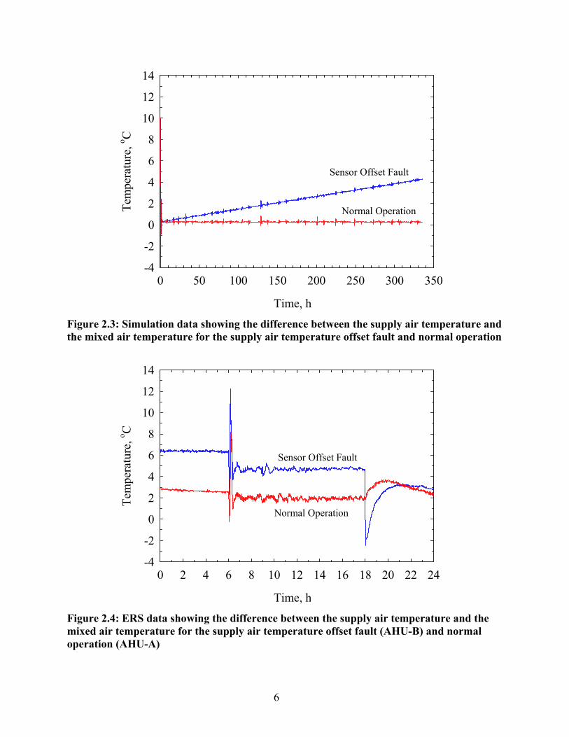
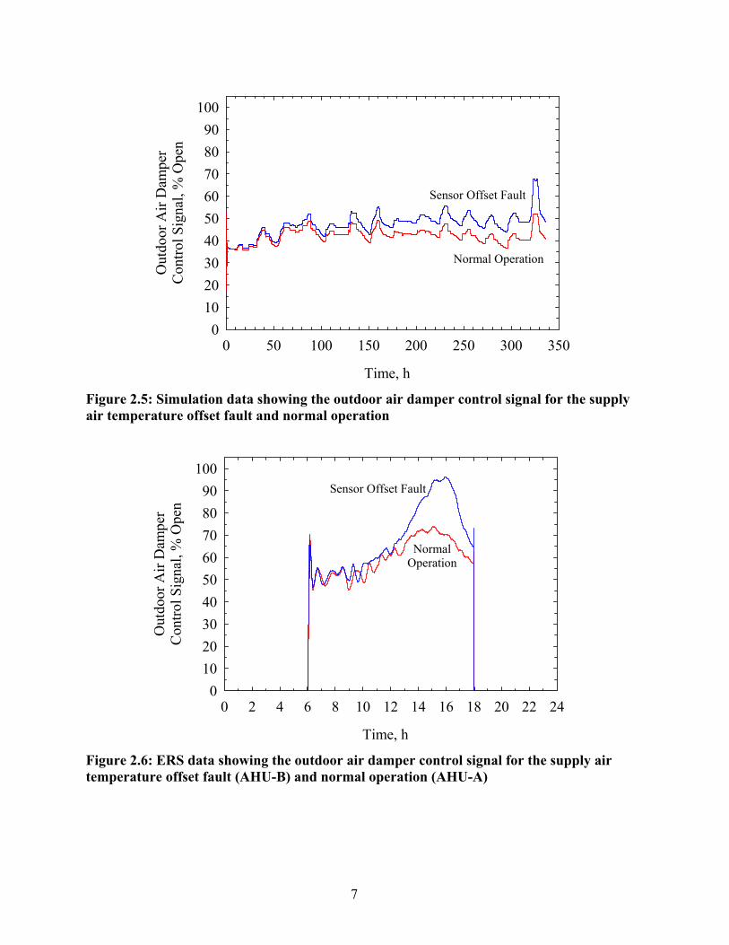
collected.) The ERS data considered were collected on January 24, 2002. Plots of the outdoor air temperature for the simulation and ERS data sets corresponding to these time periods are shown in Figures 2.1 (simulation) and 2.2 (ERS). These plots will be used to help describe the behavior of the AHUs in the presence of this and other faults where the outdoor air temperature directly impacts the conditions that are observed. Figure 2.3 shows simulation results for the difference in the supply air temperature and mixed air temperature for faulty and normal operation. For normal operation, the difference is generally less than 0.5 ºC. This difference is slightly less than what is typically seen in real equipment; however, diagnostic tools must routinely deal with uncertainties in measurements and models and the degree of this difference will not compromise the data. The fault case, on the other hand, shows the difference increasing linearly as the offset of the supply air temperature grows to 4 ºC over the two-week simulation. Figure 2.4 shows results from the ERS for the difference in the supply air temperature and mixed air temperature for faulty and normal operation. For all ERS results presented, the AHUs operate in the occupied mode from 6:00 to 18:00. During this time period, AHU-A operates normally and the difference in the supply and mixed air temperatures is approximately 2.5 ºC. AHU-B, however, has a difference of approximately 5.0 ºC in the supply and mixed air temperatures, or twice that for normal operation. The impact of the fault can also be observed in the operation of the mixing box dampers. Figure 2.5 shows the outdoor air damper control signal for the simulation fault case and for normal operation. The plot indicates that the dampers are commanded to provide additional outdoor air to be introduced for the fault case. As described previously, for the ambient conditions in the simulation, the additional outdoor air will lower the mixed air temperature and compensate for the fault (i.e., enable the supply air set point to be maintained). The effect becomes more pronounced as the offset increases over the two-week period. A similar result is found in the ERS data shown in Figure 2.6. In this case, the outdoor air damper control signal for the fault case (AHU-B) and normal operation (AHU-A) are nearly the same early in the occupied period because the outdoor air temperature is very low, ranging from –12 ºC to 0 ºC over the first 6 hours of occupancy. At these temperatures, small amounts of outdoor air are sufficient to compensate for the fault. The impact of the fault becomes evident when the outdoor temperature increases in the afternoon.

4

Time

0 50 100 150 200 250 300 350

Tem

pera

ture

, o C

-15

-10

-5

0

5

10

, hrs

Figure 2.1: Outdoor air dry-bulb temperature used for simulations for the period of February 12 to February 25, 2001

Time, hrs

0 2 4 6 8 10 12 14 16 18 20 22 24

Tem

pera

ture

, o C

-15

-10

-5

0

5

10

Figure 2.2: Outdoor air dry-bulb temperature at the ERS on January 24, 2002

5

Time

0 50 100 150 200 250 300 350

Tem

pera

ture

, o C

-4

-2

0

2

4

6

8

10

12

14

Sensor Offset Fault

Normal Operation

, hrs

Figure 2.3: Simulation data showing the difference between the supply air temperature and the mixed air temperature for the supply air temperature offset fault and normal operation

Time, hrs

0 2 4 6 8 10 12 14 16 18 20 22 24

Tem

pera

ture

, o C

-4

-2

0

2

4

6

8

10

12

14

Sensor Offset Fault

Normal Operation

Figure 2.4: ERS data showing the difference between the supply air temperature and the mixed air temperature for the supply air temperature offset fault (AHU-B) and normal operation (AHU-A)

6

Time, hrs

0 50 100 150 200 250 300 350

Out

door

Air

Dam

per

Con

trol S

igna

l, %

Ope

n

0102030405060708090

100

Sensor Offset Fault

Normal Operation

Figure 2.5: Simulation data showing the outdoor air damper control signal for the supply air temperature offset fault and normal operation

Time, hrs

0 2 4 6 8 10 12 14 16 18 20 22 24

Out

door

Air

Dam

per

Con

trol S

igna

l, %

Ope

n

0102030405060708090

100Sensor Offset Fault

NormalOperation

Figure 2.6: ERS data showing the outdoor air damper control signal for the supply air temperature offset fault (AHU-B) and normal operation (AHU-A)

7

2.1.2 Stuck Open Recirculating Air Damper This fault was simulated by setting the position of the motor driven actuator final control element for the recirculation air damper equal to one, causing the damper to stay open throughout the simulation. To implement the stuck open recirculation air damper fault at the ERS, the power supply for the damper was disconnected at the field panel. When there is no power supplied to the damper motor, the spring return on the damper motor causes the damper to go to the full open position. The damper remains at the 100 % open position for the duration of the test. Note that the outdoor air damper and exhaust air damper operate normally in the presence of this fault.

The fault causes excess return air when the AHU operates in either the free cooling mode (dampers modulate to maintain supply air temperature set point) or the mechanical cooling with 100 % outdoor air mode. For winter conditions, the AHU operates much of the time in the free cooling mode and the fault effectively raises the mixed air temperature above what would be expected at a given outdoor air damper position. To compensate, the AHU must increase the control signal to the outdoor air damper to introduce additional outdoor air to the system. The simulation was run using the February 12 to February 25, 2001 outdoor air temperature profile as input. The ERS data considered were collected on January 31, 2002. Plots of the outdoor air temperature for the simulation and ERS data sets corresponding to these time periods are presented in Figures 2.1 (simulation) and 2.7 (ERS). The impact of the fault for the simulation case is seen in Figure 2.8. The plot shows the outdoor air damper control signal for the fault case and for normal operation. The plot indicates that the dampers are commanded to provide additional outdoor air to be introduced for the fault case. The impact is the same as observed for the supply air temperature offset fault depicted in Figure 2.5, although the impact of the damper fault is more pronounced.

Time, hrs

0 2 4 6 8 10 12 14 16 18 20 22 24

Tem

pera

ture

, o C

-15

-10

-5

0

5

10

Figure 2.7: Outdoor air dry-bulb temperature at the ERS on January 31, 2002

8

Time, hrs

0 50 100 150 200 250 300 350

Out

door

Air

Dam

per

Con

trol S

igna

l, %

Ope

n

0102030405060708090

100

Stuck Open Damper Fault

Normal Operation

Figure 2.8: Simulation data showing the outdoor air damper control signal for the stuck open recirculation air damper fault and normal operation

Time, hrs

0 2 4 6 8 10 12 14 16 18 20 22 24

Out

door

Air

Dam

per

Con

trol S

igna

l, %

Ope

n

0102030405060708090

100

Normal Operation

Stuck Open Damper Fault

Figure 2.9: ERS data showing the outdoor air damper control signal for the stuck open recirculation air damper fault (AHU-A) and normal operation (AHU-B)

9

2.1.3 Leaking Heating Coil Valve This fault was implemented in the simulation code by setting the leakage parameter for the heating coil valve to several different values, causing leakage through a three-way valve of different severities. For the data considered here, a 10 % leakage fault was simulated. To implement the leaky hot-water valve fault at the ERS, a manual bypass valve was opened partially to allow hot water to be diverted around the automatic three-way bypass valve that normally controls water flow to the heating coil. An ultrasonic flow measurement device was used to determine the water flow through the heating coil. The fault was implemented to allow a leakage rate of approximately 0.019 L/s to 0.044 L/s (0.3 gal/min to 0.7 gal/min) through the coil, with a digital resolution of 0.0063 L/s (0.1 gal/min; all measurements were made in gal/min). The leakage rate is approximately 2 % to 3 % of full flow through the heating coil.

The hot-water leakage fault imposes an additional cooling load on the AHU. During the free cooling mode, the mixed air and supply air temperatures may differ significantly due to the presence of this fault. During the mechanical cooling modes (with minimum outdoor air or 100 % outdoor air), the additional load may force the cooling valve to saturate at the full open position depending on the thermal load. The impact of the fault at the ERS was quantified by establishing a fixed leakage rate and allowing the AHU to reach quasi steady-state condition in which the entering and leaving air and water temperatures and flow rates were stabilized. The unit was run with 100 % return air to help stabilize the entering air temperature. The temperature rise across the heating coil was then measured for fixed inlet water conditions to the coil and a fixed airflow rate across the coil. The fault characterization data from the ERS are provided in Table 2.1 to document the severity of the leaking valve fault in comparison to sensor faults with fixed offsets. The first column of Table 2.1 contains the leakage rate through the coil, the second column the airflow rate across the coil, and the final column the temperature rise across the coil. The heating water pump that circulates water to the heating coil operated continuously throughout the test and produced a constant flow rate of 1.65 L/s. Nearly all the water bypassed the heating coil, the exception being the small amount of leakage in column 1 of Table 2.1. The entering water temperature to the coil ranged from 60.5 ºC to 62.2 ºC during the fault characterization tests.

Table 2.1: ERS fault characterization data for AHU-B for a leaking heating coil valve fault

Water Leakage Rate (L/s)

Airflow Rate (m3/s)

Temperature Rise Across Coil (ºC)

0.032 0.80 3.1 0.032 1.61 2.1 0.044 0.80 4.6 0.044 1.62 2.8

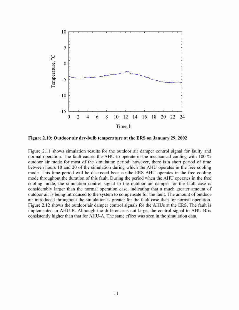
The simulation was run using the February 12 to February 25, 2001 outdoor air temperature profile as input. The ERS data considered were collected on January 29, 2002. Plots of the outdoor air temperature for the simulation and ERS data sets corresponding to these time periods are presented in Figures 2.1 (simulation) and 2.10 (ERS).

10

Time

0 2 4 6 8 10 12 14 16 18 20 22 24

Tem

pera

ture

, o C

-15

-10

-5

0

5

10

, hrs

Figure 2.10: Outdoor air dry-bulb temperature at the ERS on January 29, 2002

Figure 2.11 shows simulation results for the outdoor air damper control signal for faulty and normal operation. The fault causes the AHU to operate in the mechanical cooling with 100 % outdoor air mode for most of the simulation period; however, there is a short period of time between hours 10 and 20 of the simulation during which the AHU operates in the free cooling mode. This time period will be discussed because the ERS AHU operates in the free cooling mode throughout the duration of this fault. During the period when the AHU operates in the free cooling mode, the simulation control signal to the outdoor air damper for the fault case is considerably larger than the normal operation case, indicating that a much greater amount of outdoor air is being introduced to the system to compensate for the fault. The amount of outdoor air introduced throughout the simulation is greater for the fault case than for normal operation. Figure 2.12 shows the outdoor air damper control signals for the AHUs at the ERS. The fault is implemented in AHU-B. Although the difference is not large, the control signal to AHU-B is consistently higher than that for AHU-A. The same effect was seen in the simulation data.

11

Time

0 50 100 150 200 250 300 350

Out

door

Air

Dam

per

Con

trol S

igna

l, %

Ope

n

0102030405060708090

100Leaking Valve Fault

Normal Operation

, hrs

Figure 2.11: Simulation data showing the commanded outdoor air damper control signal for the leaking heating coil valve fault and normal operation

Time, hrs

0 2 4 6 8 10 12 14 16 18 20 22 24

Out

door

Air

Dam

per

Con

trol S

igna

l, %

Ope

n

0102030405060708090

100

Leaking Valve Fault

Normal Operation

Figure 2.12: ERS data showing the commanded outdoor air damper control signal for the leaking heating coil valve fault (AHU-B) and normal operation (AHU-A)

12

Time, h

0 50 100 150 200 250 300 350

Tem

pera

ture

, o C

-15-10-505

101520253035

Normal Operation

Leaking Valve Fault

rsFigure 2.13: Simulation data showing the difference between the supply air temperature and the mixed air temperature for the leaking heating valve fault and normal operation The impact of the fault is more pronounced when the difference in the supply air temperature and mixed air temperature is considered during the free cooling mode. Simulation results showing the difference in the supply air and mixed air temperatures for faulty and normal operation are plotted in Figure 2.13. For normal operation the difference is generally less than 0.5 ºC. For the fault case, however, the difference ranges from 6 ºC to 24 ºC. During the period noted previously when the AHU operates in the free cooling mode, the temperature difference is 18 ºC to 19 ºC. This temperature difference is too large when one considers that the supply air set point is 14 ºC to 16 ºC during this time period. The implication is that the mixed air temperature is less than 0ºC, and typical AHUs have freeze protection thermostats that shut down the unit when the mixed air temperature drops below 2 ºC to 3 ºC. To make the simulation data more realistic, the severity of the leakage should be reduced. Figure 2.14 shows results from the ERS for the difference in the supply air temperature and mixed air temperature for faulty and normal operation. AHU-A operates normally and thedifference in the supply and mixed air temperatures is approximately 2.5 ºC during the occupied period. AHU-B, however, has a difference of approximately 7.0 ºC in the supply and mixed air temperatures, or nearly three times that for normal operation. The faulty operation corresponds to a water leakage rate of approximately 0.019 L/s and an airflow rate of approximately 0.69 L/s. These conditions are slightly outside the range of those in Table 2.1; however, a slightly smaller temperature rise across the coil might have been anticipated. Nonetheless, the trend observed in the ERS data is consistent with that seen in the simulation. The primary difference is the larger impact observed in the simulation data.

13

Time, hrs

0 2 4 6 8 10 12 14 16 18 20 22 24

Tem

pera

ture

, o C

-15

-10

-5

0

5

10

15

20

25

30

Normal Operation

Leaking Valve Fault

Figure 2.14: ERS data showing the difference between the supply air temperature and the mixed air temperature for the leaking heating valve fault (AHU-B) and normal operation (AHU-A)

2.2 Variable-Air-Volume Box Faults The simulation models for two VAV box faults have been validated using data collected at the ERS. The models validated are a stuck open VAV box damper fault and a stuck open reheat valve fault. A schematic of the test room layout at the ERS is provided in Figure 2.15 to orient the reader to the matched pairs of test rooms in the facility. Data from the VAV boxes serving the test rooms are used to validate the simulation models.

2.2.1 Stuck Open VAV Box Damper This fault was simulated by setting the position of the motor driven actuator final control element for the VAV box damper equal to one, causing the damper to stay open throughout the simulation. The model includes a VAV box for each of three zones. The fault was implemented in Zone 1. The effect of the fault was studied by comparing data produced with the fault embedded in the simulation, to simulation data produced under normal operating conditions. The fault implemented at the ERS was a failed differential pressure reading, not a stuck open VAV box damper fault. The fault was implemented by disconnecting the tubing leads for the differential pressure transducer. The differential pressure is used to compute the airflow rate through the VAV box. With the tubing leads disconnected, the sensed airflow rate is zero. The controller tries to maintain the flow rate at a set point, and sensing there is no airflow rate,

14

Figure 2.15: Floor plan of the ERS showing matched pairs of test rooms.

sends a signal to the damper to open further. After a few minutes, the damper is 100 % open and remains open throughout the test. This fault has the same impact on the zone as the stuck open VAV box damper; however, two of the signatures of the fault are different. First, the airflow rate that is input to the controller is different (Note, however, that the actual airflow rate should be approximately the same since in both cases the damper is fully open). For the failed differential pressure measurement, the input is always zero. For the stuck open damper fault, the correct reading is obtained. Second, the control signal to the damper will be different under most conditions. For the failed differential pressure measurement, the control signal to the damper will always be saturated at its maximum value after the first few minutes of the fault. For the stuck

15

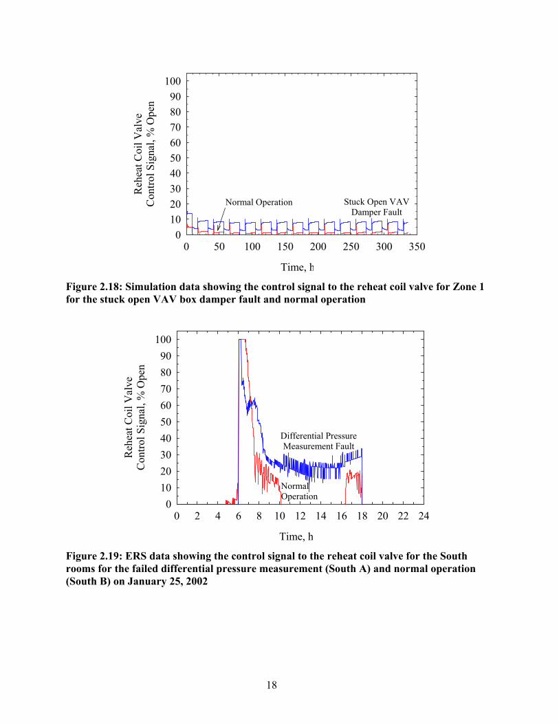
open damper fault, the control signal to the damper will be saturated at its minimum position unless the loads on the zone are such that maximum cooling is required. The effect of the damper being 100 % open (either because it is stuck or because the airflow sensor has failed) is to overcool the zone. In response, the airflow set point will be reduced to its minimum value. The fault prevents the damper from responding and, if the degree of overcooling is great enough, the controller will transition to the heating mode. The simulation was run using the February 12 to February 25, 2001 outdoor air temperature profile as input. The ERS data considered is for the South test rooms of the facility and was collected on January 25, 2002. To be consistent with the source of the data, the terminology zone will be used when referring to the simulation data and the test room name (e.g. South A, West B) will be used when referring to the ERS data. The impact of the fault for the simulation case is seen in Figure 2.16. The plot shows the airflow rate to the zone for the fault case and for normal operation. As expected, the airflow rate for the fault case is higher than the normal case throughout the simulation. Figure 2.17 shows the volumetric airflow rate for side-by-side south-facing zones with matched equipment and subject to the same external and internal loads for the fault case (South A) and normal operation (South B). Note that due to the nature of the fault in South A, the volumetric airflow rate was computed by subtracting the sum of the airflow rates to the other test rooms on AHU-A from the supply airflow rate. The effect is the same as that seen in the simulations; the test room subjected to the fault experienced larger airflow rates for the duration of the faulty operation. Another impact of the fault is seen in the use of reheat energy at the zones. Figure 2.18 shows the control signal to the reheat coil valve for Zone 1 for the fault case and normal operation. The overcooling caused by the excess air supplied to the zone for the fault case must be offset with reheat energy. Figure 2.18 shows that for the fault case, the control signal to the reheat valve is greater than that for normal operation throughout the simulation. Figure 2.19 shows a similar effect in the data obtained at the ERS. In this case, the control signal to the reheat valve for South A (failed differential pressure measurement) is greater than that for South B except for a short period of time in the morning. As in the simulation case, the fault causes South A to be overcooled requiring extra reheat energy to compensate.

16

Time, hrs

0 50 100 150 200 250 300 350

Airf

low

Rat

e, m

3 /s

0.00.10.20.30.40.50.60.70.80.91.0

Normal Operation

Stuck Open VAV Damper Fault

Figure 2.16: Simulation data showing the volumetric airflow rate to Zone 1 for the stuck open VAV box damper fault and normal operation

Time, hrs

0 2 4 6 8 10 12 14 16 18 20 22 24

Airf

low

Rat

e, m

3 /s

0.00.10.20.30.40.50.60.70.80.91.0

Differential PressureMeasurement Fault

Normal Operation

Figure 2.17: ERS data showing volumetric airflow rate to the South rooms for the failed differential pressure measurement (South A) and normal operation (South B) on January 25, 2002

17

Time, hrs

0 50 100 150 200 250 300 350

Reh

eat C

oil V

alve

Con

trol S

igna

l, %

Ope

n

0102030405060708090

100

Normal Operation Stuck Open VAVDamper Fault

Figure 2.18: Simulation data showing the control signal to the reheat coil valve for Zone 1 for the stuck open VAV box damper fault and normal operation

Time, hrs

0 2 4 6 8 10 12 14 16 18 20 22 24

Reh

eat C

oil V

alve

Con

trol S

igna

l, %

Ope

n

0102030405060708090

100

Differential PressureMeasurement Fault

NormalOperation

Figure 2.19: ERS data showing the control signal to the reheat coil valve for the South rooms for the failed differential pressure measurement (South A) and normal operation (South B) on January 25, 2002

18

2.2.2 Stuck Open VAV Box Reheat Valve The simulated fault was implemented by setting the position of the motor driven actuator final control element for the VAV box reheat coil control valve equal to one, causing the valve to stay open throughout the simulation. The fault was implemented in the VAV box serving Zone 1. To implement the stuck open VAV box reheat valve fault at the ERS, a control voltage from a source independent of the control system was applied to the reheat coil valve actuator in West A. Unlike the simulation case in which the valve was stuck 100 % open, the fault implemented at the ERS had a small magnitude. The valve was stuck only slightly open, producing a flow rate through the valve of approximately 1.7e-2 L/s, whereas maximum flow is approximately 20 times this value. The effect of the fault is the same (i.e., the valve can not open or close) from the standpoint of the trends that are observed in the data and, therefore, the data can be used to validate the simulation model. Beyond this use, however, the more subtle effect of the fault implemented at the ERS will pose a greater challenge when the data are used to test the ability of diagnostic tools to detect the presence of the fault.

Depending on the zone (test room) conditions and the severity of the fault, the stuck reheat valve either creates an additional cooling load that the air-handling unit must try to remove, or it prevents the valve from modulating to provide additional heating energy to the zone. In the first case, the controller increases the airflow rate to the zone in an attempt to compensate for the fault. If the fault is severe, the zone temperature will gradually increase beyond the zone set point. In the second case, the zone temperature will tend to gradually decrease below the zone set point. The impact of the fault at the ERS was quantified by establishing a fixed input voltage to the reheat valve and a fixed airflow rate through the VAV box, and then measuring the entering and leaving water and air temperatures, and the water and air flow rates. The fault characterization data from the ERS are provided in Table 2.2 to document the severity of the fault. Column one of Table 2.2 lists the water leakage rate, column two the room airflow rate, and column three the temperature rise across the reheat coil. The entering water temperature to the reheat coil ranged from 57.4 ºC to 58.7 ºC during the fault characterization testing. Table 2.2 indicates that, as expected, the temperature rise of the air moving across the reheat coil increases as the water leakage rate increases.

19

Time, hrs

0 50 100 150 200 250 300 350

Airf

low

Rat

e, m

3 /s

0.0

0.1

0.2

0.3

0.4

0.5

0.6

Stuck Open Reheat Valve Fault

Normal Operation

Figure 2.20: Simulation data showing the volumetric airflow rate for Zone 1 for the stuck open VAV box reheat valve fault and normal operation

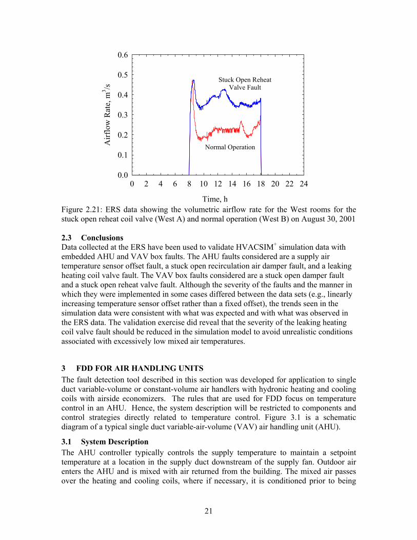
The simulation was run using the July 12 to July 25, 2001 outdoor air temperature profile as input. The ERS data considered were collected on August 30, 2001. Figure 2.20 shows simulation results for faulty and normal operation. The fault causes the damper to open fully in an effort to maintain the zone temperature at the set point. Hence, the airflow rate for the fault case is consistently higher than the airflow rate for normal operation. Figure 2.21 shows a similar effect for the data from the ERS. The hot water flow rate through the coil was approximately 0.022 L/s. From Table 2.2, a temperature rise across the coil of approximately 5 ºC is expected. From Figure 2.23 the actual airflow rate is roughly 40 % higher than the value in Table 2.2 (approximately 0.4 m3/s compared to 0.28 m3/s), so the temperature rise across the coil would be somewhat less if all other inlet conditions were unchanged.

20

Time

0 2 4 6 8 10 12 14 16 18 20 22 24

Airf

low

Rat

e, m

3 /s

0.0

0.1

0.2

0.3

0.4

0.5

0.6

Normal Operation

Stuck Open ReheatValve Fault

, hrsFigure 2.21: ERS data showing the volumetric airflow rate for the West rooms for the stuck open reheat coil valve (West A) and normal operation (West B) on August 30, 2001 2.3 Conclusions Data collected at the ERS have been used to validate HVACSIM+ simulation data with embedded AHU and VAV box faults. The AHU faults considered are a supply air temperature sensor offset fault, a stuck open recirculation air damper fault, and a leaking heating coil valve fault. The VAV box faults considered are a stuck open damper fault and a stuck open reheat valve fault. Although the severity of the faults and the manner in which they were implemented in some cases differed between the data sets (e.g., linearly increasing temperature sensor offset rather than a fixed offset), the trends seen in the simulation data were consistent with what was expected and with what was observed in the ERS data. The validation exercise did reveal that the severity of the leaking heating coil valve fault should be reduced in the simulation model to avoid unrealistic conditions associated with excessively low mixed air temperatures.

3 FDD FOR AIR HANDLING UNITS The fault detection tool described in this section was developed for application to single duct variable-volume or constant-volume air handlers with hydronic heating and cooling coils with airside economizers. The rules that are used for FDD focus on temperature control in an AHU. Hence, the system description will be restricted to components and control strategies directly related to temperature control. Figure 3.1 is a schematic diagram of a typical single duct variable-air-volume (VAV) air handling unit (AHU).

3.1 System Description The AHU controller typically controls the supply temperature to maintain a setpoint temperature at a location in the supply duct downstream of the supply fan. Outdoor air enters the AHU and is mixed with air returned from the building. The mixed air passes over the heating and cooling coils, where if necessary, it is conditioned prior to being

21

supplied to the building. The typical operating sequence for AHUs consists of four primary modes of operation during occupied periods for maintaining the supply air temperature and the ventilation at preset levels. The relationship of the four operating modes to the control of the heating coil valve, the cooling coil valve and the mixing box dampers is shown in Figure 3.2. Sequencing logic determines the mode of operation as dictated by various thermal relationships including the internal and external loads on the zones served by the AHU.

C

C

ReturnFan

RecirculationAir Damper

Normally Open

Exhaust Air DamperNormally Closed

CoolingCoil

HeatingCoil

Filter

H

C

SupplyFan

T & H

T & H

Return Air

DamperMotor

Air Handling Controller

Outputs

Inputs

Outdoor Air DamperNormally Closed

FromZones

ToZones

T

Outdoor Air Temperature& Humidity Sensors

TMixed

Air

SupplyAir

Figure 3.1: Schematic diagram of a single duct air-handling unit

Mode 2 Mode 3 Mode 4Mode 1

Con

trol S

igna

l (%

) 100

0

HeatingCoil Valve

CoolingCoil ValveMixing Box

Dampers

Mode 2 Mode 3 Mode 4Mode 1

Con

trol S

igna

l (%

) 100

0

HeatingCoil Valve

CoolingCoil ValveMixing Box

Dampers

Figure 3.2: Typical operating modes of an air-handling unit

22

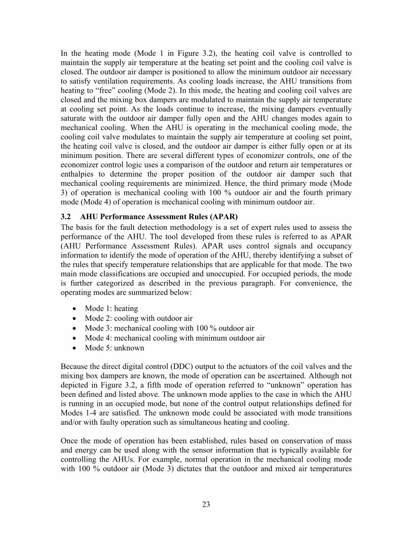
In the heating mode (Mode 1 in Figure 3.2), the heating coil valve is controlled to maintain the supply air temperature at the heating set point and the cooling coil valve is closed. The outdoor air damper is positioned to allow the minimum outdoor air necessary to satisfy ventilation requirements. As cooling loads increase, the AHU transitions from heating to “free” cooling (Mode 2). In this mode, the heating and cooling coil valves are closed and the mixing box dampers are modulated to maintain the supply air temperature at cooling set point. As the loads continue to increase, the mixing dampers eventually saturate with the outdoor air damper fully open and the AHU changes modes again to mechanical cooling. When the AHU is operating in the mechanical cooling mode, the cooling coil valve modulates to maintain the supply air temperature at cooling set point, the heating coil valve is closed, and the outdoor air damper is either fully open or at its minimum position. There are several different types of economizer controls, one of the economizer control logic uses a comparison of the outdoor and return air temperatures or enthalpies to determine the proper position of the outdoor air damper such that mechanical cooling requirements are minimized. Hence, the third primary mode (Mode 3) of operation is mechanical cooling with 100 % outdoor air and the fourth primary mode (Mode 4) of operation is mechanical cooling with minimum outdoor air.

3.2 AHU Performance Assessment Rules (APAR) The basis for the fault detection methodology is a set of expert rules used to assess the performance of the AHU. The tool developed from these rules is referred to as APAR (AHU Performance Assessment Rules). APAR uses control signals and occupancy information to identify the mode of operation of the AHU, thereby identifying a subset of the rules that specify temperature relationships that are applicable for that mode. The two main mode classifications are occupied and unoccupied. For occupied periods, the mode is further categorized as described in the previous paragraph. For convenience, the operating modes are summarized below:

Mode 1: heating • • • • •

Mode 2: cooling with outdoor air Mode 3: mechanical cooling with 100 % outdoor air Mode 4: mechanical cooling with minimum outdoor air Mode 5: unknown

Because the direct digital control (DDC) output to the actuators of the coil valves and the mixing box dampers are known, the mode of operation can be ascertained. Although not depicted in Figure 3.2, a fifth mode of operation referred to “unknown” operation has been defined and listed above. The unknown mode applies to the case in which the AHU is running in an occupied mode, but none of the control output relationships defined for Modes 1-4 are satisfied. The unknown mode could be associated with mode transitions and/or with faulty operation such as simultaneous heating and cooling. Once the mode of operation has been established, rules based on conservation of mass and energy can be used along with the sensor information that is typically available for controlling the AHUs. For example, normal operation in the mechanical cooling mode with 100 % outdoor air (Mode 3) dictates that the outdoor and mixed air temperatures

23

must be approximately equal. Defining Toa and Tma as the outdoor air and mixed air temperatures, respectively, the rule (defined as Rule 10) is written as

Rule 10: |Toa - Tma| > εt

where εt is a threshold that depends on the uncertainty (or accuracy) of the measurements. The rules are written such that a fault is indicated if a rule is true. In the example above, the rule states that the outdoor and mixed air temperatures are not the same (i.e., if true, a fault has occurred). House et al. [5] provide a detailed description of the 28 APAR rules and the reasoning behind them. For this reason, the rules are simply listed in Table 3.1 without detailed explanation. Table 3.1 groups the rules according to mode of operation. As indicated in the column heading for the rule expression, a true expression is indicative of a fault. Nomenclature for the rule set is provided in the Appendix to this report. Table 3.2 presents the rules as related groups and indicates the sensors and control signals used to evaluate each rule. The first group of rules treats the relationship of temperatures in the coil subsystem of the AHU. For these four rules, only the relational operator in the rules change from one mode to another. A typical rule from this subgroup requires the supply air temperature to be lower than the sum of the mixed air temperature and the temperature rise across the supply fan in the mechanical cooling modes. There are also groups of rules treating the mixing box subsystem, the zone subsystem, economizer operation, comfort requirements, and controller logic/tuning. Hence, although there are 28 rules, in reality only a small number of temperature and control signal relationships are used to define the rules. With the possible exception of the mixed air temperature, this information is generally available for most AHUs controlled with a DDC system. If one or more sensors are not available, certain rules will no longer be applicable. For instance, in the absence of a mixed air temperature sensor, nine rules listed in Table 3.2 (Rules 1, 2, 7, 10, 11, 16, 18, 26, and 27) will be eliminated from consideration in APAR. Conversely, the presence of additional sensors would expand the rule set and provide an opportunity to either detect more faults, or to detect faults during modes of operation in which they would normally be hidden. For instance, if a temperature sensor was installed between the heating and cooling coils, leakage through the heating valve could be detected during the mechanical cooling modes, whereas normally it would be masked in these modes.

24

Table 3.1: APAR Rule Set Mode Rule # Rule Expression (true implies existence of a fault)

1 Tsa < Tma + ∆Tsf - εt

2 For |Tra - Toa| ≥ ∆Tmin: |Qoa/Qsa - (Qoa/Qsa)min | > εf

3 |uhc – 1| ≤ εhc and Tsa,s – Tsa ≥ εt Heating

4 |uhc – 1| ≤ εhc

5 Toa > Tsa,s - ∆Tsf + εt

6 Tsa > Tra - ∆Trf + εt Cooling with Outdoor Air

7 |Tsa - ∆Tsf - Tma| > εt

8 Toa < Tsa,s - ∆Tsf - εt

9 Toa > Tco + εt

10 |Toa - Tma| > εt

11 Tsa > Tma + ∆Tsf + εt

12 Tsa > Tra - ∆Trf + εt

13 |ucc – 1| ≤ εcc and Tsa – Tsa,s ≥ εt

Mechanical Cooling with 100 % Outdoor Air

14 |ucc – 1| ≤ εcc

15 Toa < Tco - εt

16 Tsa > Tma + ∆Tsf + εt 17 Tsa > Tra - ∆Trf + εt

18 |Tra - Toa| ≥ ∆Tmin

19 |ucc – 1| ≤ εcc and Tsa – Tsa,s ≥ εt

Mechanical Cooling with Minimum Outdoor Air

20 |ucc – 1| ≤ εcc

21 ucc > εcc and uhc > εhc and εd < ud < 1 - εd

22 uhc > εhc and ucc > εcc

23 uhc > εhc and ud > εd

Unknown Occupied Modes

24 εd < ud < 1 - εd and ucc > εcc

25 | Tsa – Tsa,s | > εt

26 Tma < min(Tra , Toa) - εt

27 Tma > max(Tra , Toa) + εt

All Occupied Modes

28 Number of mode transitions per hour > MTmax

25

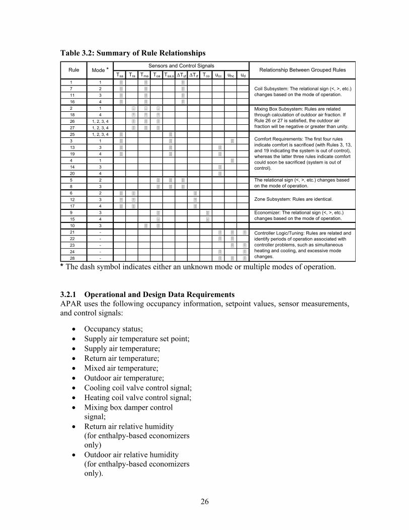
Table 3.2: Summary of Rule Relationships

Tsa Tra Tma Toa Tsa,s ∆Tsf ∆Trf Tco ucc uhc ud

1 17 211 316 42 118 426 1, 2, 3, 427 1, 2, 3, 425 1, 2, 3, 43 113 319 44 114 320 45 28 36 212 317 49 315 410 321 -22 -23 -24 -28 -

Controller Logic/Tuning: Rules are related and identify periods of operation associated with controller problems, such as simultaneous heating and cooling, and excessive mode changes.

Coil Subsystem: The relational sign (<, >, etc.) changes based on the mode of operation.

Comfort Requirements: The first four rules indicate comfort is sacrificed (with Rules 3, 13, and 19 indicating the system is out of control), whereas the latter three rules indicate comfort could soon be sacrificed (system is out of control).

The relational sign (<, >, etc.) changes based on the mode of operation.

Zone Subsystem: Rules are identical.

Economizer: The relational sign (<, >, etc.) changes based on the mode of operation.

Mixing Box Subsystem: Rules are related through calculation of outdoor air fraction. If Rule 26 or 27 is satisfied, the outdoor air fraction will be negative or greater than unity.

Sensors and Control SignalsRelationship Between Grouped RulesRule Mode *

* The dash symbol indicates either an unknown mode or multiple modes of operation. 3.2.1 Operational and Design Data Requirements APAR uses the following occupancy information, setpoint values, sensor measurements, and control signals:

• Occupancy status; • Supply air temperature set point;

• Supply air temperature; • Return air temperature; • Mixed air temperature; • Outdoor air temperature; • Cooling coil valve control signal; • Heating coil valve control signal; • Mixing box damper control

signal; • Return air relative humidity

(for enthalpy-based economizers only)

• Outdoor air relative humidity (for enthalpy-based economizers only).

26

In addition to the operational data listed above, certain design data are needed to implement the rules. The required design data are:

Minimum and maximum values of control signals for the heating coil valve, cooling coil valve and mixing box dampers for normalizing the control signals;

•

• •

•

• • • • •

•

Percentage outdoor air necessary to satisfy ventilation requirements; Changeover temperature from mechanical cooling with 100 % outdoor air to mechanical cooling with minimum outdoor air (or equivalent condition for enthalpy-based economizer); Description of sequencing/economizer cycle strategy.

The description of the sequencing/economizer cycle strategy is used to verify that the rules are suitable to a particular AHU installation. 3.2.2 Detecting and Diagnosing Faults APAR can be used to detect faults; however, a specific set of faults that can be identified has not been established. Rather, any fault that causes a rule to be satisfied would be detected and additional effort would be necessary to isolate the source of the problem. Faults that could potentially be identified by the rule set include the following:

Stuck or leaking mixing box dampers, heating coil valves, and cooling coil valves; Temperature sensor faults; Design faults such as undersized coils; Sequencing logic errors; Central plant faults affecting the hot or chilled water supply conditions at the AHU coils; Inappropriate operator intervention.

The operating point, severity of a fault, and threshold selection for the rules will obviously influence when a particular rule is satisfied. Threshold selection is discussed next. 3.2.3 Threshold Selection In addition to the sensor, control signals, and setpoint information, other parameters must be specified for APAR. For instance, estimates of the temperature rise across the supply fan (and return fan, if one exists) must be provided, a reasonable default is 1.1 ºC. A model-based value correlated to the airflow rate or the control signal to the fan could be used as the basis for this estimate; however, some amount of training data would likely be necessary to establish the correlation. Thresholds used in evaluation of rules such as εt in Rule 10 must also be specified. A value of 1.7 ºC is typically used for all rules involving the comparison of temperatures. These threshold values (and several others used in APAR) is currently determined heuristically. A more rigorous approach that is being considered would involve determining the uncertainty associated with each temperature measurement and then combining the uncertainty terms to produce the most conservative representation of each rule. Such an approach would tend to produce rules that are both

27

sensitive to faults and robust against false alarms. As an example, the threshold in Rule 10 would be determined from the expression

εt = εToa + εTma

where εToa and εTma

are the uncertainties associated with the measurement of the outdoor and mixed air temperatures. Typical values of other threshold parameters used in APAR are listed below (see rule set in Table 3.1 and nomenclature in Attachment A):

• εt = 1.7 ºC • εf = 0.3 • εcc = εd = εhc = 0.02 • ∆Tsf = ∆Trf = 1.1 ºC • ∆Tmin = 5.6 ºC • (Qoa/Qsa) min = 0.1 • MTmax = 6

3.3 Instrumentation Accuracy Requirements APAR uses existing sensor points in the building automation system (BAS) to perform the fault detection calculations. The typical industrial grade sensors that are already installed for control purposes have sufficient accuracy. Laboratory grade instruments are not required.

3.4 Results from AHU Laboratory Experiments In Section 2.1 the implementation procedures for three AHU faults that were examined at the ERS were described. Two to three days of data were typically collected for each of the faults (supply air temperature sensor offset, stuck open recirculation air damper, and leaking heating coil valve) for both summer and winter conditions. The temperature sensor offset fault was implemented with a 1.7 ºC offset (stage 1 fault) and a 2.8 ºC offset (stage 2 fault). The leaking heating coil valve fault was implemented with a leakage rate of 0.019 L/s (stage 1 fault), 0.032 L/s (stage 2 fault), and 0.044 L/s (stage 3 fault). For the summer conditions, the occupied period was 8:00 AM to 6:00 PM, whereas occupancy began at 6:00 AM for the winter conditions. Results obtained from processing the ERS data with APAR are presented in Table 3.3 (summer conditions) and Table 3.4 (winter conditions). The first column in the tables represent the operation state of the AHU. Where applicable, the stage of the fault is provided in the second column. The AHU being tested, the date, the number of hours the fault was active, the APAR rule satisfied and the number of hours satisfied are presented in columns three through six. The operation state is either normal or one of the three faults. Other operational problems could arise during testing; however, with the exception of a few hours of problems noted in the discussion below, there is no indication that they did.

28

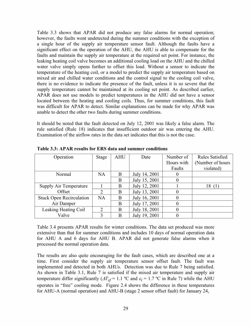
Table 3.3 shows that APAR did not produce any false alarms for normal operation; however, the faults went undetected during the summer conditions with the exception of a single hour of the supply air temperature sensor fault. Although the faults have a significant effect on the operation of the AHU, the AHU is able to compensate for the faults and maintain the supply air temperature at the required set point. For instance, the leaking heating coil valve becomes an additional cooling load on the AHU and the chilled water valve simply opens further to offset this load. Without a sensor to indicate the temperature of the heating coil, or a model to predict the supply air temperature based on mixed air and chilled water conditions and the control signal to the cooling coil valve, there is no evidence to indicate the presence of the fault, unless it is so severe that the supply temperature cannot be maintained at its cooling set point. As described earlier, APAR does not use models to predict temperatures in the AHU did not have a sensor located between the heating and cooling coils. Thus, for summer conditions, this fault was difficult for APAR to detect. Similar explanations can be made for why APAR was unable to detect the other two faults during summer conditions. It should be noted that the fault detected on July 12, 2001 was likely a false alarm. The rule satisfied (Rule 18) indicates that insufficient outdoor air was entering the AHU. Examination of the airflow rates in the data set indicates that this is not the case.

Table 3.3: APAR results for ERS data and summer conditions

Operation Stage AHU Date Number of Hours with

Faults

Rules Satisfied (Number of hours

violated) B July 14, 2001 0 Normal NA B July 15, 2001 0

1 B July 12, 2001 1 18 (1) Supply Air Temperature Offset 2 B July 13, 2001 0

B July 16, 2001 0 Stuck Open Recirculation Air Damper

NA B July 17, 2001 0

2 B July 18, 2001 0 Leaking Heating Coil Valve 3 B July 19, 2001 0

Table 3.4 presents APAR results for winter conditions. The data set produced was more extensive than that for summer conditions and includes 10 days of normal operation data for AHU A and 6 days for AHU B. APAR did not generate false alarms when it processed the normal operation data. The results are also quite encouraging for the fault cases, which are described one at a time. First consider the supply air temperature sensor offset fault. The fault was implemented and detected in both AHUs. Detection was due to Rule 7 being satisfied. As shown in Table 3.1, Rule 7 is satisfied if the mixed air temperature and supply air temperature differ significantly (∆Tsf = 1.1 ºC and εt = 1.7 ºC in Rule 7) while the AHU operates in “free” cooling mode. Figure 2.4 shows the difference in these temperatures for AHU-A (normal operation) and AHU-B (stage 2 sensor offset fault) for January 24,

29

Table 3.4: APAR results for ERS data and winter conditions

Operation Stage AHU Date Number of Hours with

Faults

Rules Satisfied (Number of hours

violated) A Jan. 22, 2002 0 B Jan. 22, 2002 0 A Jan. 23, 2002 0 A Jan. 24, 2002 0 A Jan. 25, 2002 0 A Jan. 26, 2002 0 A Jan. 27, 2002 0 A Jan. 28, 2002 0 A Jan. 29, 2002 0 B Jan. 30, 2002 0 B Jan. 31, 2002 0 B Feb. 1, 2002 0 A Feb. 2, 2002 0 B Feb. 2, 2002 0 A Feb. 3, 2002 0

Normal NA

B Feb. 3, 2002 0 B Jan. 23, 2002 10 7 (10) 1 A Jan. 30, 2002 8 7, 25 (6, 2) *

Supply Air Temperature Offset

2 B Jan. 24, 2002 11 7 (11) B Jan. 25, 2002 11 8, 10 (4, 11) B Jan. 26, 2002 8 8, 10 (3, 8)

Stuck Open Recirculation Air Damper NA

A Jan. 31, 2002 11 8, 10 (11, 11) 2 B Jan. 27, 2002 4 8, 11 (4, 3) 3 B Jan. 28, 2002 11 24, 28 (5, 6) 1 B Jan. 29, 2002 11 7 (11)

Leaking Heating Coil Valve

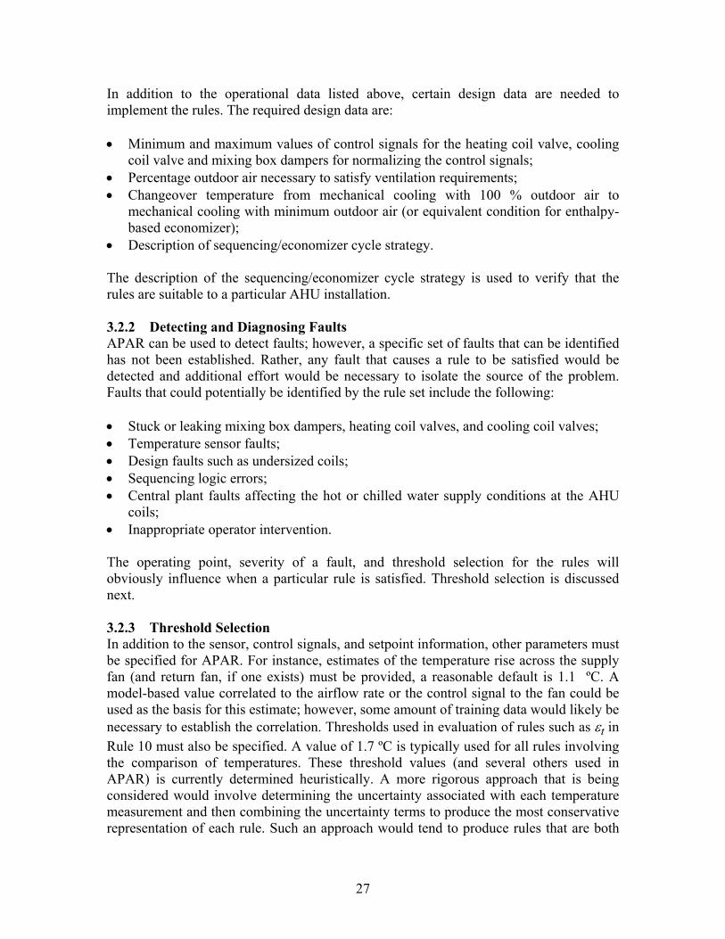
2 A Feb. 1, 2002 9 7, 25, 27 (8, 1, 1) * 7, 25 (6, 2) denotes that Rule 7 was satisfied for 6 h and Rule 25 was satisfied for 2 h. 2002. The impact of the fault is evident in Figure 2.4 and the presence of a fault is correctly identified by APAR. Recall that APAR does not perform diagnostics; it simply suggests possible explanations why a rule might be satisfied. A temperature sensor error is one possible reasons provided by APAR to explain why Rule 7 might be satisfied. Table 3.4 indicates that Rule 25 is satisfied for 2 hours when the sensor offset fault is implemented in AHU-A. This rule is satisfied when the supply air temperature is not maintained at the set point. In fact, the fault occurred because the AHU was not running, but the problem was actually caused by the outdoor air damper. It failed to open when it was initially commanded to do so, and then opened abruptly, drawing in excessive outdoor air and causing the mixed air temperature to drop significantly. The cold air tripped the freezestat and shut the unit down.

30

The next fault considered is the stuck open recirculation air damper. The fault was introduced and detected in both AHUs for winter conditions. Table 3.4 indicates that Rules 8 and 10 were satisfied due to the effects of the fault. Both rules apply to operation in the mechanical cooling with 100 % outdoor air mode. Rule 8 is satisfied if the outdoor air temperature is low enough to enable “free” cooling with outdoor air. Rule 10 is satisfied if the outdoor air temperature and mixed air temperature differ significantly. For winter conditions, the fault causes warmer recirculation air to be mixed with outdoor air, resulting in a mixed air temperature that is significantly higher than expected (Operation with 100 % outdoor air is expected to result in a mixed air temperature that is nearly equal to the outdoor air temperature.). The impact of the fault can be seen in Figure 3.3. For the first several hours of the day, the outdoor air temperature is well below the supply air temperature set point of 12.8 ºC. Hence, outdoor air alone can provide the necessary cooling load. The figure also reveals that the mixed and outdoor air temperatures differ by 4.0 ºC or more over the entire day. This is more than twice the allowable difference established by the rule threshold of 1.7ºC. The final fault considered is the leaking heating valve fault. Table 3.4 indicates that Rules 8 and 11 are satisfied for the January 27, 2002 data. Both rules apply to the mechanical cooling with 100 % outdoor air mode. As shown in Figure 3.4, the outdoor air temperature is sufficiently low to enable cooling with outdoor air for much of the morning. Hence, Rule 8 is satisfied. Rule 11 is satisfied when the supply air temperature is significantly higher than the mixed air temperature. This should only happen in the heating mode. Although not shown in Figure 3.4, the mixed air temperature is nearly the same as the outdoor air temperature over the entire day because the unit operates with 100 % outdoor air. By comparing the outdoor air temperature and supply air temperature, it is evident that Rule 11 is satisfied for several hours in the morning. APAR lists a leaking heating coil valve as one of the possible explanations for Rules 8 and 11 being satisfied. The leaking heating valve fault data for January 29, 2002 and February 1, 2002 result in Rule 7 being satisfied for most of those two days. Recall that Rule 7 is satisfied if the supply and mixed air temperatures differ significantly while the unit operates in the cooling with outdoor air mode. The presence of a leaking valve fault is one of the reasons this type of operational behavior might be observed. The data for February 1, 2002 also include one hour during which Rules 25 and 27 were satisfied. These rules were satisfied because a freezestat trip occurred similar to the one described previously. The data from January 28, 2002 resulted in several hours of violations of Rules 24 and 28. The control of AHU-B was very unstable that day. In particular, the oscillation of the dampers was extreme and persistent over a 5 hour to 6 hour period. Eventually the dampers stabilized, but they did so at a partially open position. Simultaneously the cooling coil valve was modulating to maintain the supply air temperature at the set point. Rule 28 was satisfied due to excessive mode switching caused by the unstable behavior. Rule 24 was satisfied due to the simultaneous modulation of the dampers and the cooling coil valve.

31

Time (hh:mm)

00:00 04:00 08:00 12:00 16:00 20:00 00:00

Tem

pera

ture

, o C

-5

0

5

10

15

20

25Mixed Air Temperature

Outdoor Air Temperature

Occupied Period

Figure 3.3: Stuck open recirculation damper fault for winter conditions (AHU-B, January 25, 2002)

Time (hh:mm)

00:00 04:00 08:00 12:00 16:00 20:00 00:00

Tem

pera

ture

, o C

-5

0

5

10

15

20

25

30

Occupied Period

Supply AirTemperature Set Point

Outdoor AirTemperature

Supply AirTemperature

Figure 3.4: Leaking heating coil valve fault for winter conditions (AHU-B, January 27, 2002)

32

3.5 Results from APAR Analysis of AHU Simulation Data Using HVACSIM+ Simulation, as described in section 2, was used to test and refine APAR. The simulation consisted of a single floor in a commercial office building with a VAV AHU and three VAV boxes. The faults selected for simulation are those that typically occur in AHUs and include sensor drifts, stuck or leaking dampers, and stuck or leaking valves. Each simulation was run for a two-week period, including a range of fault types and fault severities. In Table 3-5 the first four columns list the fault identification number along with descriptions of the component affected, the type of error simulated, and the respective fault condition. The last three columns of Table 3.5 list the results of the APAR analysis for heating season, swing season, and cooling season. In this table, a dash denotes that no fault was detected.

Table 3.5: Fault Description and APAR Detection Results for Simulated Data

APAR Rule Violated Fault ID Component Fault

Type Fault

Condition Heating Swing Cooling 0 Fault free none none - - - 1 Supply air temp. sensor zero drift (0 to -4) ºC 7 5,7 - 2 zero drift (0 to +4) ºC 7 - - 3 Return air temp. sensor zero drift (0 to -4) ºC - - 18 4 zero drift (0 to +4) ºC - - 26 5 Mixed air temp. sensor zero drift (0 to -4) ºC 7 7,10,26 10,18,26 6 zero drift (0 to +4) ºC 7 7,10 10,18,27 7 Outdoor air temp. sensor zero drift (0 to -4) ºC - 10 10,27 8 zero drift (0 to +4) ºC - 5,10,26 10 10 Outdoor air damper stuck closed - 10 - 15 Recirculating air damper stuck closed - - 18,19,25 16 leakage 10 % - - - 18 leakage 40 % - 10 - 19 Cooling coil valve stuck closed - 13,25 12,13 20 leakage 10 % 1 1,5,7,24,25 - 21 leakage 25 % 28 1,5,7,25,28 1,5,7, 25 22 leakage 40 % 28 1,5,7,24,25,28 1,5,7,17,2523 Heating coil valve stuck closed - - - 24 leakage 10 % 7,8,11 8 - 25 leakage 25 % 8,11 8,11 19,20,25 26 leakage 40 % 8,11 8,11,24 19,25 27 VAV box damper stuck open - - - 28 stuck closed - 28 - 29 VAV reheat valve stuck open - 25 - 30 stuck closed - - -

33

3.5.1 Normal Operation The simulation was carried out using weather data representing cooling, heating, and swing seasons. Specifically, two weeks of actual weather data from the “Weather Year for Energy Calculation” tape were selected from the months of July, October, and February, respectively. The APAR tool produced no false alarms for normal data, regardless of the season tested. This result confirms that the system is not violating any of the applied rules. The simulated control system tested here operates on a simple control loop. First, the outdoor and return air enthalpies are compared to determine whether it is beneficial to operate the economizer. If the answer is yes, the damper is modulated based on an algorithm that uses the supply air temperature measurement as an input. Other methods of control that use the mixed air, outdoor air, or return air conditions to modulate the damper position were not tested. This has a large impact on both the response of the system to simulated faults as well as the ability of APAR to detect a fault as is presented in the discussion below. 3.5.2 Simulated Faults The following subsections will first describe the faults tested, provide a brief explanation of the expected outcome, and then the actual test results will be presented and discussed. 3.5.2.1 Supply Air Temperature Sensor Drift (Faults 1 & 2) The sensor drift for the supply air temperature sensor was introduced as a sensor offset for a range of (0 to -4) ºC, applied linearly over the two-week simulation period. The effect of the negative sensor offset would result in a increased recirculation air temperature as the control logic seeks to lower the supply air temperature to meet the setpoint. However, if the supply air setpoint target is met, the actual supply air temperature would be lower and the VAV box controls would have to compensate. First, the VAV box dampers would close, and if the temperature to the zone is still too low, then the reheat coil would be activated. This type of fault would typically be masked in a system without diagnostic capabilities and results in increased energy use. The simulation uses the supply air temperature as a direct input to the system control; therefore this fault has a significant impact on the system operation even at low fault levels. For all seasons, the controller works to reverse the decreasing temperature reading for Fault 1 (Figure 3.5). In heating season this is achieved by damper modulation, closing the damper in response to the negative sensor drift of Fault 1 and as a result the mixed air temperature is too high relative to the supply air temperature reading that triggers a fault. Similarly, in swing season negative sensor drift is detected. In cooling season, the economizer is called on earlier and the cooling coil valve signal is reduced to bring the supply air temperature to the setpoint. The actual supply air temperature will be too high and may make it difficult to meet the zone setpoint temperatures but APAR detects no fault. However, if the VAV box damper is not able to maintain the zone temperature, a reset of the supply air temperature setpoint to a lower setting will be triggered.

34

Figure 3.5: Heating Season Simulation Data Showing the Change to Damper Position and Mixed Air Temperature Due to Fault 1 A second simulation was carried out to introduce a sensor offset in the range of (0 to +4) ºC. For Fault 2, a positive sensor offset would prompt the control logic to lower the supply air temperature. The VAV box controls would work to compensate. First, the VAV box dampers would open. As the severity of this type of fault is increased, the thermal comfort in the room would be compromised and the condition of the high zone temperature and open dampers would trigger a reset of the supply air temperature to a lower setpoint. In simulation, Fault 2 was detected for heating mode when the damper controller opens to reduce the supply air temperature, causing the mixed air temperature to drop out of range. For swing season there is a missed alarm, no fault is detected though the damper responds by opening and the mixed air temperature drops. In cooling season, the economizer is called on later and the cooling coil valve signal is increased to bring the supply air temperature to the setpoint. The actual supply air temperature will be too low and will require reheat at VAV box but APAR detects no fault. 3.5.2.2 Return Air Temperature Sensor Drift (Faults 3 & 4) Return air temperature sensor drift was introduced as a sensor offset for a range of (0 to +4) ºC, also applied linearly over the two-week simulation period. In this simulation, the return air temperature measurement is used in the determination for economizer use, but not for damper control. Therefore, for heating and swing season, where the cooling load

35

conditions are such that the economizer is meeting the cooling load, the control is unaffected. The change in the measurement of the return air temperature does not trigger an APAR rule violation. In cooling season, the outdoor air enthalpy is higher and therefore the perceived reduction in return air temperature causes the economizer to be called on later but with the low outdoor air fraction, APAR warns that energy may be wasted by not using economizer (Rule 18). This type of fault would not affect thermal comfort, as the supply air temperature will be met by mechanical cooling. However, additional cooling load is being introduced to the building and thereby resulting in increased energy use. A second simulation, Fault 4, was carried out to introduce a sensor offset in the range of (0 to –4) ºC. The effect of negative sensor drift for the return air temperature with no change to the humidity reading would result in a reduced recirculation air enthalpy. This false reading is input to the economizer control and depending on the operating conditions, the controller may open the recirculation air damper while reducing the outdoor air damper position to the minimum setting. The system may stop use of the economizer due to the false readings and switch to mechanical cooling with minimum outdoor air. For Fault 4, control in heating and swing season is unaffected and the increase in return temperature does not trigger an APAR rule violation. For cooling season, the economizer use is extended and APAR detects that the mixed air temperature reading is lower than outdoor air temperature or return air temperature and triggers violation of Rule 26. This type of fault would also not effect thermal comfort as the supply air temperature will be met, but energy use is increased. 3.5.2.3 Mixed Air Temperature Sensor Drift (Faults 5 & 6) Mixed air temperature sensor drift was introduced as a sensor offset for a range of (0 to +4) ºC, also applied linearly over the two-week simulation period. The mixed air temperature measurement is also used in the determination for economizer use, but not for damper control. In this case, control is unaffected regardless of season. However, for heating and swing season the change in the measurement of the mixed air temperature relative to the supply air temperature reading does trigger an APAR rule violation (Rule 7). In Mode 3, it is expected that the mixed air temperature will closely track the outdoor air temperature and that the mixed air temperature will be greater than the outdoor or return air temperatures. Because these statements were not true, Rules 10 and 26 were violated in the swing and cooling seasons. A related Rules 18 is also violated in cooling season. For Fault 6, a simulation was carried out to introduce a sensor offset in the range of(0 to –4) ºC which shows that a similar pattern exists due to the positive sensor drift. Once again control is unaffected, but the relationships between the temperature measurements cause several rule violations.

36

3.5.2.4 Outdoor Air Temperature Sensor Drift (Faults 7 & 8) Outdoor air temperature sensor drift was introduced as a sensor offset for a range of (0 to –4) ºC, also applied linearly over the two-week simulation period. The outdoor air temperature measurement is used in the determination for economizer use, but not for damper control. Therefore, for heating season, the control is unaffected and the change in the measurement of the outdoor air temperature does not trigger an APAR rule violation. In swing season, control is still unaffected because the economizer is still in use, but the perceived difference between the outdoor air temperature and the mixed air temperature is too great when considering that the outdoor air damper is fully opened. APAR detects this condition and determines that Rule 10 has been violated. In cooling season, the perceived outdoor air enthalpy is lower and therefore the perceived reduction in outdoor air temperature causes the economizer to be cut off later. For swing and cooling season, APAR detects the Rule 10 violation and also determines that in cooling season the mixed air temperature is reading higher than the return air temperature and the outdoor air temperature, a violation of Rule 27. A second simulation, Fault 8, was carried out to introduce a sensor offset in the range of (0 to +4) ºC. In this simulation, control in heating and swing season is unaffected as the outdoor air temperature sensor reading increases. For cooling season, the economizer use is reduced because of the perception that the outdoor air temperature has increased. APAR is able to detect this fault in all cases except for heating mode. In cooling and swing season there is at least one day where the damper is commanded to be fully open and APAR detects that difference between the outdoor air temperature and the mixed air temperature is not reasonable, violating Rule 10. 3.5.2.5 Outdoor Air Damper Fault (Fault 10) This fault was introduced to the outdoor air damper by setting the control signal for the motor-driven actuator to the stuck closed position, causing the damper to stay at the minimum open position throughout the simulation. The result of this is that no economizer action can be taken and mechanical cooling will have to be used exclusively. The control system response for this fault was varied. In heating season, the damper opening is increased from 40 % open to 80 % open. In swing season, the damper opening was also increased, and over several days the cooling coil is activated. In cooling season, the control system calls for mechanical cooling with minimum outdoor air. Therefore, the system is insensitive to the fault. APAR was only able to detect a rule violation for Fault 10 in swing season because it expects the mixed air temperature and the outdoor air temperature to be roughly equal for conditions of 100 % outdoor air. In heating season, the damper is not called to be fully open and in cooling season, the economizer cycle is off. 3.5.2.6 Recirculating Air Damper (Faults 15-16) This fault was introduced to the recirculation air damper by setting the control signal for the motor-driven actuator to three different levels: stuck open, 40 %, 10 % leakage, and stuck closed.

37

The stuck closed recirculation air damper fault causes the damper position to prevent air from being recirculated. For the case of free cooling with 100 % outdoor air, the recirculation damper is already closed. For conditions that the outdoor enthalpy is higher than the return air enthalpy, the system is not operating under the economizer cycle, the outdoor air damper would be set to its minimum, and the fault would cause the recirculation damper to be closed, hence the airflow may be reduced. This was only evident during cooling season where Faults 18, 19 and 25 were triggered. In the two-week simulations for both heating and swing season, the stuck closed recirculation damper had no effect on the control system response and was not detected by APAR. The simulation runs at 40 % leakage and 10 % leakage are meant to test the ability of the fault detection and diagnostic tool to detect lower level faults. In the case that the return air enthalpy is greater than that of the outdoor air, additional cooling will be required. However, the 10 % and 40 % leakage simulations caused no notable change to the control, regardless of season. Furthermore, the only rule violated was during swing season when it was detected that the outdoor air temperature did not match the mixed air temperature. This fault does not apply to the summer conditions when the economizer cycle is not used. 3.5.2.7 Cooling Coil Valve Faults (Faults 19-22) This fault was introduced to the cooling coil valve by setting the control signal for the motor-driven valve actuator to four different levels: stuck closed, 10 % leakage, 25 % leakage, and 40 % leakage. The various leakage rates are meant to test the sensitivity of the fault detection tool. The cooling coil is needed to maintain the supply air temperature setpoint when cooling with outdoor air is insufficient. The stuck closed cooling coil valve fault causes the valve position to prevent cold water from being circulated through the cooling coil. This fault is easily detected when the cooling load is high, primarily swing season and cooling season. Looking at the APAR results, it is shown that Fault 19 is not detected during heating season. This is logical because the heating season cooling load is met by use of the economizer having low outdoor temperatures. As the seasonal temperatures are higher for swing season and cooling season, the cooling coil valve is called open. APAR also identifies that the control system is not meeting the cooling load in swing season and cooling season while the cooling coil signal is not at a maximum. During swing season and cooler outdoor air conditions, the economizer can provide sufficient cooling. Therefore, having a leaking cooling coil valve will cause the supply air temperature to drop and the VAV box reheat coil would have to be activated to bring the temperature up to the zone setpoint. This represents a tremendous waste of energy as the cooling coil and reheat coil are working against each other. For the leaking cooling coil faults, the control system calls for an end to economizer operation and activation of the heating coil valve. In all cases, control of the heating coil becomes unstable for fault 21 and 22. Various rule violations are reported, showing that many of the expected temperature relationships are not being met. In addition the system is incapable of

38

maintaining the supply air temperature setpoint. This type of fault could go undetected in a system because unless the leak is larger than the heating capacity of the reheat coil, the zone temperature will be maintained. 3.5.2.8 Heating Coil Valve Faults (Faults 23-26) These faults were introduced to the heating coil valve by setting the control signal for the motor-driven valve actuator to four different levels: stuck closed, 10 % leakage, 25 % leakage, and 40 % leakage. The various leakage rates are meant to test the sensitivity of the fault detection tool. The heating coil valve is not activated due to cold weather conditions, rather the heating coil valve is opened when the system is at risk of freezing or if a cooling coil leak exists. Therefore, Fault 23, a stuck heating coil valve causes the valve position to prevent hot water from being circulated through the heating coil but affects no change to the control of the air handling unit and furthermore was not detected by the APAR fault detection tool. In contrast, even a 10 % valve leakage caused the dampers to be fully open, during heating and swing season to make use of the economizer cycle and additionally called for the cooling coil valve to be activated. For cooling season, the economizer is off and the cooling coil must meet the full cooling load. As the severity of the fault increased to 25 %, the control system response during heating and swing season shows a further opening of the cooling coil valve. For the cooling season, the cooling coil was at its maximum open position and the supply air temperature was not maintained, which is noted by the violation of Rule 19. 3.5.2.9 VAV Box Faults (Faults 27-30) Although the VAV box faults are downstream of the air handling unit, APAR was used to evaluate the operational data to determine whether the tool was robust enough to pick up any faults. APAR is not designed or intended to reliably detect faults in the attached VAV boxes, but may be useful in identifying when a problem exists outside of the air handling unit. The results shown in Table 3.5 show that in swing season there were two faults that caused an APAR rule violation. The first evidence of faulty operation came from the VAV box damper stuck closed. It shows Rule 28 was violated. It is not evident whether the operating point caused the excessive mode switches, or if in fact the closed damper reduced the airflow to a level that the system began to fluctuate between modes of operation in an effort to maintain the supply set point. The second evidence of faulty operation was detected for the reheat valve stuck open. In this case we see that the system is unable to maintain the supply temperature setpoint. 3.6 Results from AHU Emulation in the VCBT Emulation, using the VCBT as described in section 2, was used in addition to simulation, to test and refine APAR. The emulation consisted of two floors in a commercial office building with a VAV AHU and three VAV boxes for each floor.

39

3.6.1 Faults Implemented The faults tested in emulation were selected to represent common faults that had potential to be detected using typical sensor measurements. 3.6.1.1 Supply Air Temperature Sensor Drift The occurrence of sensor drift for the supply air temperature sensor was introduced as a sensor offset for a range of (0 to –4) ºC, applied linearly over the two-week simulation period. A negative sensor offset would prompt the control logic to raise the supply air temperature. The VAV box controls will work to compensate. First, the VAV box dampers will open. As the severity of this type of fault is increased, the thermal comfort in the room is compromised and the condition of the high zone temperature and open dampers will trigger a reset of the supply air temperature to a lower setpoint. 3.6.1.2 Outdoor Air Temperature Sensor Drift The outdoor air temperature sensor is an input to the economizer control. It is used to calculate the outdoor air enthalpy which is compared to the recirculation air enthalpy. The effect of negative sensor drift for the outdoor air temperature with no change to the humidity reading would result in an increased outdoor air enthalpy. 3.6.1.3 Stuck Outdoor Air Damper This fault was introduced to the outdoor air damper by setting the control signal for the motor-driven actuator to the stuck closed position, causing the damper to stay at the minimum open position throughout the simulation. The result of this is that no economizer action can be taken and mechanical cooling will have to be used exclusively. 3.6.1.4 Stuck Recirculation Air Damper This fault was introduced to the recirculation air damper by setting the control signal for the motor-driven actuator to stuck open. This allows excess return air to be recirculated and mixed with the outdoor air in the free cooling mode or mechanical cooling with 100 % outdoor air. For conditions that the outdoor enthalpy is lower than the return air enthalpy, the control system will have to respond by further opening the outdoor air damper. 3.6.1.5 Stuck Cooling Coil Valve This fault was introduced to the cooling coil valve by setting the control signal for the motor-driven valve actuator to four different levels: stuck closed, 10 % leakage, 25 % leakage, and 40 % leakage. During swing season and cooler outdoor air conditions, the economizer can provide sufficient cooling. Therefore, having a leaking cooling coil valve will cause the supply air temperature to drop and the VAV box reheat coil would have to be activated to bring the temperature up to the zone setpoint. This represents a tremendous waste of energy as the cooling coil and reheat coil are working against each other. This type of fault could go undetected in a system because unless the leak is larger than the heating capacity of the reheat coil, the zone temperature will be maintained. The 10 %, 25 %, and 40 % leakage rates are meant to test the sensitivity of the fault detection tool.

40

3.6.2 Normal Operation Normal data was collected for the two AHUs in heating season, swing season, and cooling season. These data represents the “no fault” case and is used as a benchmark for comparison to faulty data. One week of normal data was collected in real time for each of these cases. Expert knowledge of the system combined with the trending data from the input signals to the control system was used to verify the system response. In Figure 3.6, the top graph shows the input temperatures during typical operation in heating season for Controller A. This data show the natural fluctuations in outdoor air temperature, and the ability of the control system to maintain the temperature setpoint within an allowable threshold. The lower graph in the Figure 3.6 shows the control system response to control the cooling coil, heating coil and outdoor air damper position. Here it is evident that even in heating season, the heating coil valve is closed and the building cooling load is met by use of the enthalpy-based economizer. The economizer determines the enthalpy of the return air and outdoor air to determine whether it is advantageous to use outdoor air to provide the needed cooling. For the weather conditions selected to represent heating season, we see that a 40 % to 60 % damper position is selected and the system is “free” cooling which is designated as Mode 2 (Fig 3.2). For Controller B, identical weather data is used. The only difference is the control logic used to maintain the setpoint temperature; Controller A controls the system based on the supply air temperature reading while Controller B controls based on the outdoor, return, and mixed air conditions. For Controller B, the supply air and the mixed air temperature are almost the same over the range of operating conditions and for the occupied periods, there is significantly less fluctuation of the damper position. For swing season, the outdoor air no longer provides sufficient cooling to meet the buildings cooling load. This weather data triggers the control system to open the outdoor air damper to maximum when the outdoor air enthalpy is less than the return air enthalpy, and in addition, the cooling coil valve position is opened as required. The data shown in Figure 3.7 for controller B is similar to data from controller A. The last season evaluated was the cooling season. No fault cases were evaluated in cooling season, however, it was

41

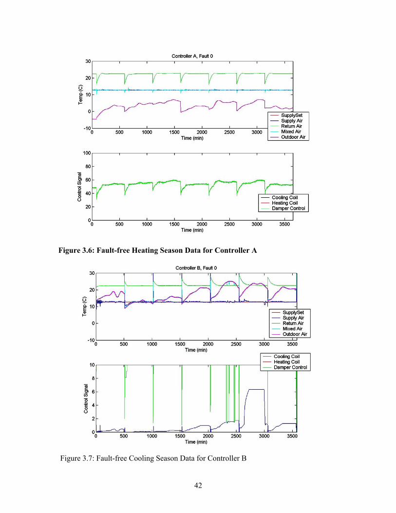
Figure 3.6: Fault-free Heating Season Data for Controller A

Figure 3.7: Fault-free Cooling Season Data for Controller B

42

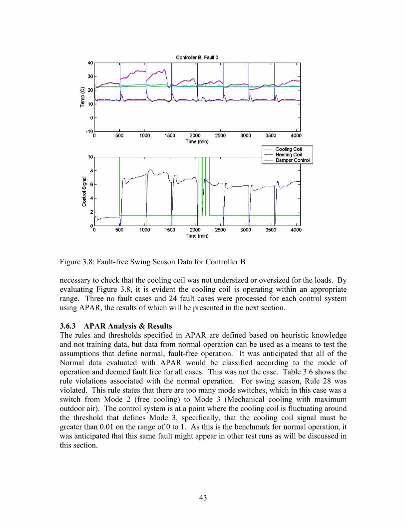
Figure 3.8: Fault-free Swing Season Data for Controller B necessary to check that the cooling coil was not undersized or oversized for the loads. By evaluating Figure 3.8, it is evident the cooling coil is operating within an appropriate range. Three no fault cases and 24 fault cases were processed for each control system using APAR, the results of which will be presented in the next section. 3.6.3 APAR Analysis & Results The rules and thresholds specified in APAR are defined based on heuristic knowledge and not training data, but data from normal operation can be used as a means to test the assumptions that define normal, fault-free operation. It was anticipated that all of the Normal data evaluated with APAR would be classified according to the mode of operation and deemed fault free for all cases. This was not the case. Table 3.6 shows the rule violations associated with the normal operation. For swing season, Rule 28 was violated. This rule states that there are too many mode switches, which in this case was a switch from Mode 2 (free cooling) to Mode 3 (Mechanical cooling with maximum outdoor air). The control system is at a point where the cooling coil is fluctuating around the threshold that defines Mode 3, specifically, that the cooling coil signal must be greater than 0.01 on the range of 0 to 1. As this is the benchmark for normal operation, it was anticipated that this same fault might appear in other test runs as will be discussed in this section.

43

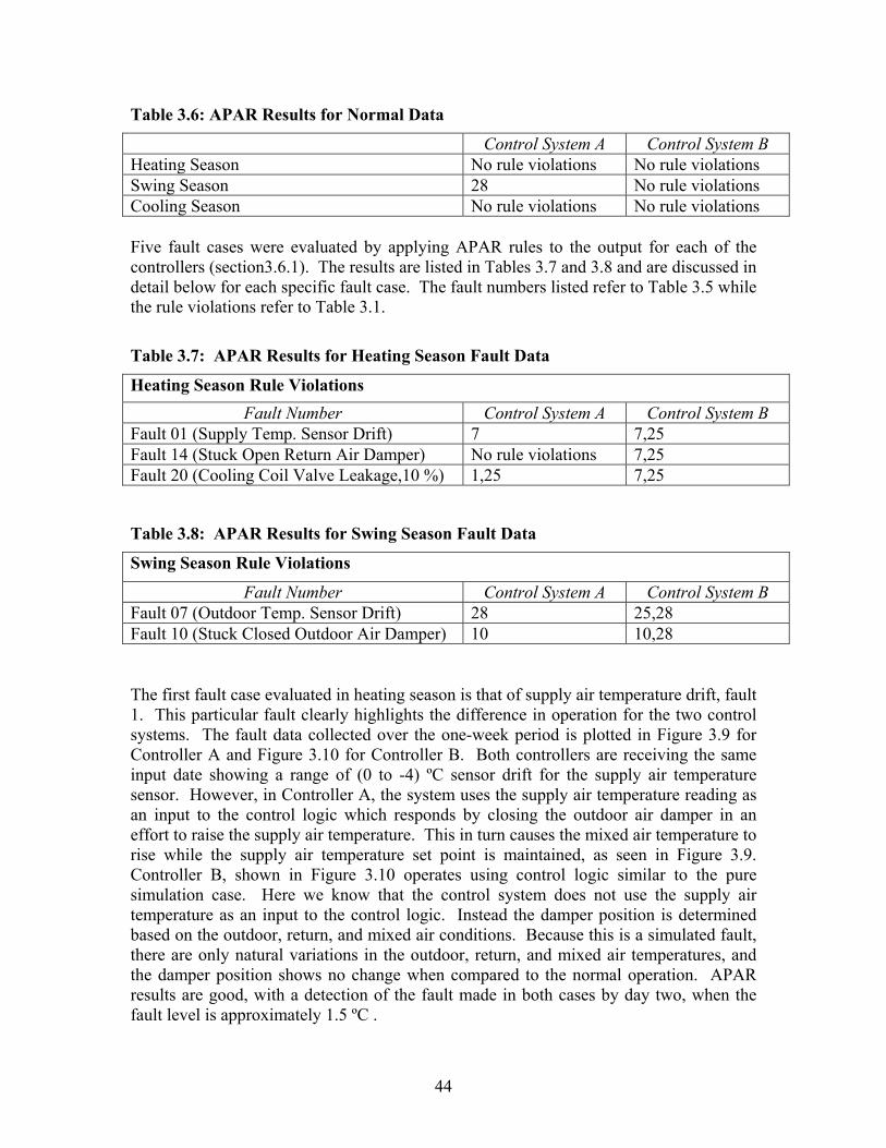
Table 3.6: APAR Results for Normal Data

Control System A Control System B Heating Season No rule violations No rule violations Swing Season 28 No rule violations Cooling Season No rule violations No rule violations Five fault cases were evaluated by applying APAR rules to the output for each of the controllers (section3.6.1). The results are listed in Tables 3.7 and 3.8 and are discussed in detail below for each specific fault case. The fault numbers listed refer to Table 3.5 while the rule violations refer to Table 3.1.

Table 3.7: APAR Results for Heating Season Fault Data

Heating Season Rule Violations Fault Number Control System A Control System B

Fault 01 (Supply Temp. Sensor Drift) 7 7,25 Fault 14 (Stuck Open Return Air Damper) No rule violations 7,25 Fault 20 (Cooling Coil Valve Leakage,10 %) 1,25 7,25

Table 3.8: APAR Results for Swing Season Fault Data

Swing Season Rule Violations

Fault Number Control System A Control System B Fault 07 (Outdoor Temp. Sensor Drift) 28 25,28 Fault 10 (Stuck Closed Outdoor Air Damper) 10 10,28 The first fault case evaluated in heating season is that of supply air temperature drift, fault 1. This particular fault clearly highlights the difference in operation for the two control systems. The fault data collected over the one-week period is plotted in Figure 3.9 for Controller A and Figure 3.10 for Controller B. Both controllers are receiving the same input date showing a range of (0 to -4) ºC sensor drift for the supply air temperature sensor. However, in Controller A, the system uses the supply air temperature reading as an input to the control logic which responds by closing the outdoor air damper in an effort to raise the supply air temperature. This in turn causes the mixed air temperature to rise while the supply air temperature set point is maintained, as seen in Figure 3.9. Controller B, shown in Figure 3.10 operates using control logic similar to the pure simulation case. Here we know that the control system does not use the supply air temperature as an input to the control logic. Instead the damper position is determined based on the outdoor, return, and mixed air conditions. Because this is a simulated fault, there are only natural variations in the outdoor, return, and mixed air temperatures, and the damper position shows no change when compared to the normal operation. APAR results are good, with a detection of the fault made in both cases by day two, when the fault level is approximately 1.5 ºC .

44

Figure 3.9: Fault 1 Heating Season Data for Controller A

Figure 3.10: Fault 1 Heating Season Data for Controller B

45

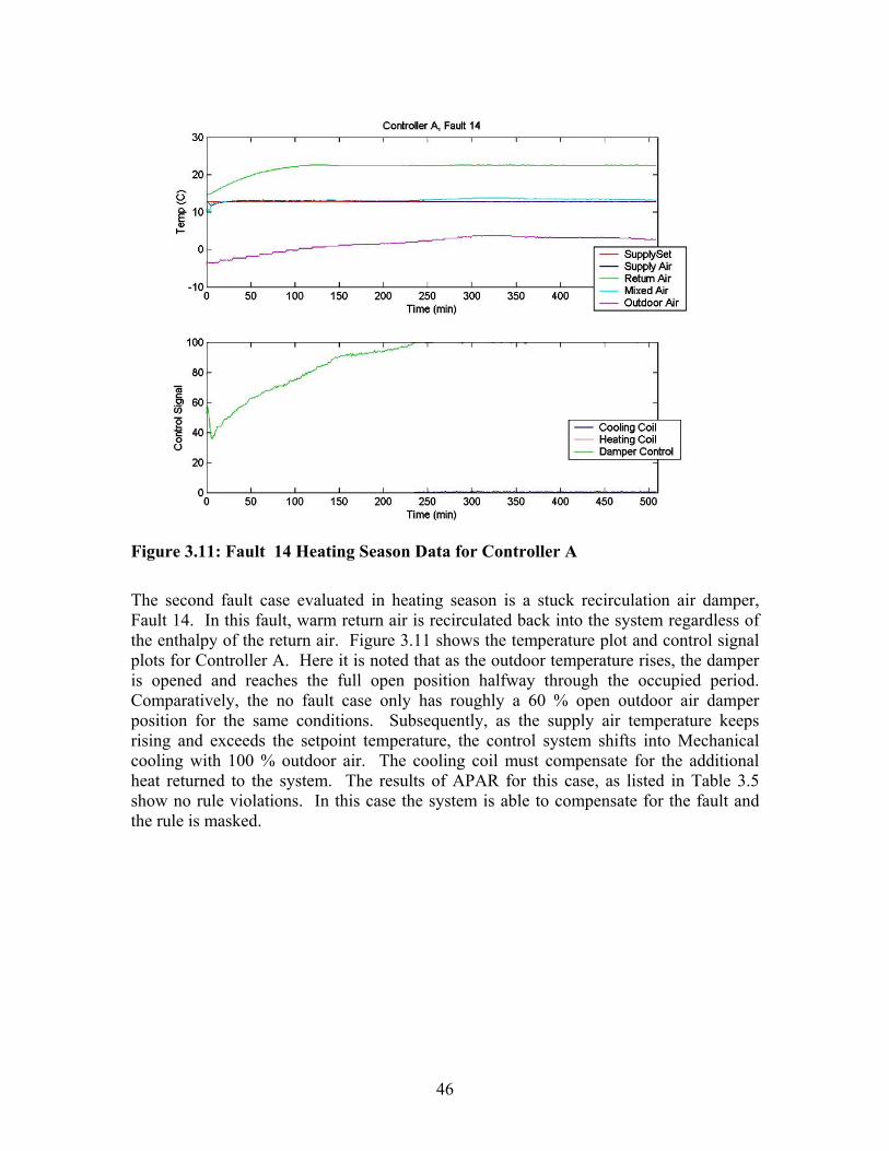
Figure 3.11: Fault 14 Heating Season Data for Controller A The second fault case evaluated in heating season is a stuck recirculation air damper, Fault 14. In this fault, warm return air is recirculated back into the system regardless of the enthalpy of the return air. Figure 3.11 shows the temperature plot and control signal plots for Controller A. Here it is noted that as the outdoor temperature rises, the damper is opened and reaches the full open position halfway through the occupied period. Comparatively, the no fault case only has roughly a 60 % open outdoor air damper position for the same conditions. Subsequently, as the supply air temperature keeps rising and exceeds the setpoint temperature, the control system shifts into Mechanical cooling with 100 % outdoor air. The cooling coil must compensate for the additional heat returned to the system. The results of APAR for this case, as listed in Table 3.5 show no rule violations. In this case the system is able to compensate for the fault and the rule is masked.

46

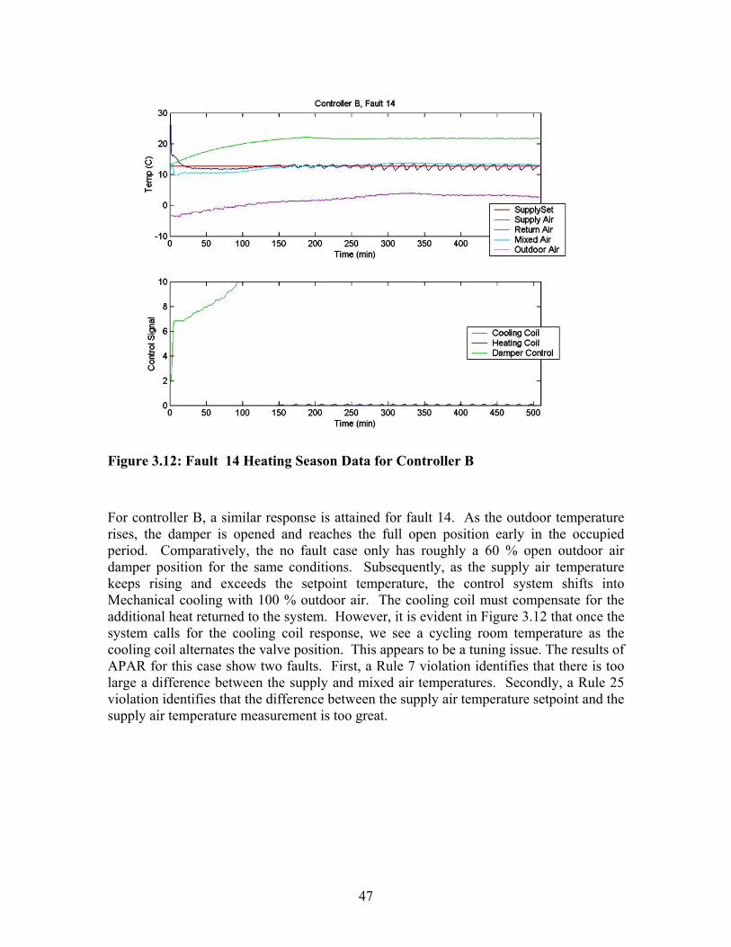
Figure 3.12: Fault 14 Heating Season Data for Controller B For controller B, a similar response is attained for fault 14. As the outdoor temperature rises, the damper is opened and reaches the full open position early in the occupied period. Comparatively, the no fault case only has roughly a 60 % open outdoor air damper position for the same conditions. Subsequently, as the supply air temperature keeps rising and exceeds the setpoint temperature, the control system shifts into Mechanical cooling with 100 % outdoor air. The cooling coil must compensate for the additional heat returned to the system. However, it is evident in Figure 3.12 that once the system calls for the cooling coil response, we see a cycling room temperature as the cooling coil alternates the valve position. This appears to be a tuning issue. The results of APAR for this case show two faults. First, a Rule 7 violation identifies that there is too large a difference between the supply and mixed air temperatures. Secondly, a Rule 25 violation identifies that the difference between the supply air temperature setpoint and the supply air temperature measurement is too great.

47

Figure 3.13: Fault 20 Heating Season Data for Controller A The third fault case evaluated in heating season is that of stuck cooling coil valve, Fault #20. The response for Controller A is shown in Figure 3.13. Under the fault condition, the 10 % valve leakage causes the damper to change from 50 % open to its minimum position. This provides 15 % outdoor air and 85 % return air. In the top graph we see that the mixed air temperature closely tracks the return air temperature. However, the temperature of the supply air is lower than the supply air temperature setpoint and the heating coil must be activated at a level of approximately 15 %. APAR results show Rule 1 and Rule 25 violations for Controller A. The Rule 1 violation shows that the supply and mixed air temperature do not correlate in the heating mode. This is the expected alarm. In addition the Rule 25 violation shows that the control system was unable to maintain the setpoint. Controller B finds the same rule violations, but applied to Mode 2 because the controller is cooling with outdoor air. The response for Controller B is not shown because the control logic does not control based on supply air temperature and therefore behaves as if there is no fault. The only symptom that appears is that the supply air temperature drops as a result of the cooling coil leak. In a real world application, the reheat coil at the VAV boxes would have to compensate by adding heat. This represents very expensive and inefficient operation, as use of the reheat coil is an expensive way to counteract the fault.

48

Figure 3.14: Fault 7 Swing Season Data for Controller B The first fault case evaluated in swing season is that of outdoor air temperature drift, fault 07. Both controllers are receiving the same input date showing a range of (0 to -4) ºC sensor drift for the outdoor air temperature sensor. However, in Controller A, the system uses the supply air temperature reading as an input and therefore a false reading at the outdoor air temperature is not expected to be detected. The results however, show a rule 28 violation. This violation states that the allowable number of mode transitions per hour has been exceeded. This is a tuning issue. For Controller B the system control is determined based on the condition of the outdoor, return, and mixed air, similar to the pure simulation case. The fault data collected Controller B over the one-week period is plotted in Figure 3.14. It shows that as the fault level increases, the system begins to have difficulty maintaining the setpoint. This triggers a violation of rule 25, where the supply air temperature is not equal to the supply air setpoint. In addition, for selected ranges of operation APAR detected excessive mode switching.

49

Figure 3.15: Fault 10 Swing Season Data for Controller B

The second fault case evaluated in swing season is that of stuck closed outdoor air damper, fault 10. When the outdoor air damper is stuck closed, only the minimum ventilation of 15 % enters the building. The rest is made up of return air, which has a higher temperature than the outdoor air for most of the simulation days. This fault effectively disables the economizer from making use of free cooling. As a result, the damper is commanded open earlier than for the no fault condition, and there is increased cooling coil activity to bring the return air temperature to the supply air temperature setpoint, as seen in Figure 3.15. APAR results for this data show one rule violation, Rule 10 for both controllers. This rule states that there is an unexpected difference in the mixed air temperature and the outdoor temperature. In Mode 3, mechanical cooling with 100 % outdoor air, the outdoor air should be roughly equal to the mixed air. APAR finds that this is not the case for Controller A and Controller B, triggering faults in each case. In addition, for Controller B, a Rule 28 violation signals excessive mode switching. Upon further analysis, it is determined that the cause of this is the fluctuation of the cooling coil valve when the load is slightly larger than the economizer can handle with free cooling. This mode switching violation is one that has proven recurrent in swing season data.

50

3.7 APAR User Interface The user interface is instrumental to the successful application of an FDD method. This section will present FDD_AHU1.1, which is a front end to the APAR code which was developed by the Centre Scientifique et Technique du Bâtiment [3]. It enables batch processing of system data and in the future will be improved to process on-line streaming data. To evaluate the user interface and test the implementation of APAR, archived AHU data from Montgomery College was processed and the output compared to output produced by a separate implementation of APAR [5]. The test case used to develop this interface uses data from two air-handling units. Data are imported as a text file and processed to detect and diagnose faults. Figure 3.16 shows the files available for import. The naming convention for the imported data files is significant because the first two characters in the name represent the type of air-handling unit being evaluated. In this example, it is air-handler 1, denoted by “a1”. The corresponding rules differ slightly depending on the AHU number because some units use an enthalpy-based economizer while others use a temperature-based economizer. The information regarding the type of air-handlers being evaluated is selected in the initial software setup.

Figure 3.16: FDD_AHU Import Data Figure 3.17: FDD_AHU Fault List

This software is designed to implement the APAR rules, which define temperature relationships in the AHU that are dependent on the mode of operation. If a rule is satisfied, a fault is indicated, but there is no diagnosis of the exact nature of the fault. Within the program, users are capable of enabling or disabling rules. S specific faults can be deselected so the corresponding rule is not evaluated and therefore does not trigger an alarm. This feature, shown in Figure 3.17, is useful when service has already been called regarding a specific fault because it gives users the ability to acknowledge receipt of the alarm status and remove it from evaluation as the rest of the system is checked.

51

Once the data is imported and the evaluation criteria are selected, the analysis can be run by clicking the “go” button. This processes the data for the week and generates a color coded one-week calendar that summarizes the operation of a given AHU for that week (see Figure 3.18). Three levels of granularity can be shown within this one-week calendar. Days with no faults are white. Days with 1hour to 4 hours of faults are colored beige. Finally, days with more than 5 hours of faults are colored red. It should be pointed out that the APAR rules are evaluated hourly, so the presence of two faults indicates that there were two hours of operation during that day that represented faulty operation. This user interface has the capability to present information both temporally (a number of days of operation is shown rather than a snapshot of current operation) and spatially (a number of AHUs can be shown simultaneously to understand how their operation compares).

igure 3.18: Summary of Fault Detection Results for One-week Data

igure 3.19 illustrates results for one day (Monday) selected from week 12 of year 2000.

F FHere a color coded key shows the periods of faulty, unknown, and fault free operation along with the mode of operation associated with a particular hour within a day. The first row lists the time of day while the second row shows the dominant fault cause by number. Fault causes are provided in a list at the bottom of the window. Also shown in this window are the mode of operation and operating condition for each hour of the day. Note that “multiple modes” of operation indicates that the mode switched at least once in that hour. If the mode switches too often (more than six times for all data considered

52

Figure 3.19: Summary of Fault Detection Results and Possible Causes

Figure 3.20: Temperature graph

53

Figure 3.21: Control signal graph here), a fault is indicated. Otherwise, hours that have multiple modes of operation are indicated to be normal. The three buttons to the right side of the window, “Details”, “Graphic T” and “Graphic CMD” provide a greater depth of information for the user. The details window, not shown here, is a text file listing the specific hours where faults were detected and the associated causes. The “Graphics T” window (see Figure 3.20) shows a temperature versus time plot for several key sensors while the “Graphic CMD” window (see Figure 3.21) shows the relevant control signals. This is intended as a troubleshooting tool for users and is also useful in debugging the software to ensure that the logic is applied correctly.

54

4 FDD FOR VAV 4.1 VAV box Performance Assessment Control Charts - VPACC The primary purpose of heating, ventilating, and air-conditioning (HVAC) equipment in commercial buildings is to provide a comfortable and healthy environment for occupants. Variable-air-volume (VAV) air handling systems are common for conditioning air and delivering the air to occupied zones. VAV boxes are an integral part of such systems and are the final piece of equipment that air passes through prior to reaching the occupants. As such, it is important to ensure that these devices operate correctly. The challenges presented in detecting and diagnosing faults in VAV boxes are similar to those encountered with other pieces of HVAC equipment. Generally there are very few sensors, making it difficult to ascertain what is happening in the device. Limitations associated with controller memory and communication capabilities further complicate the task. The number of different types of VAV boxes and lack of standardized control sequences add a final level of complexity to the challenge. This set of constraints is counterbalanced by the fact that VAV boxes are much more numerous than other pieces of HVAC equipment. For instance, buildings may have ten to fifteen times more VAV boxes than air-handling units. Hence, maintenance staffs would clearly benefit from a tool that assisted them in monitoring VAV box operation. The needs and constraints described above have led to the development of VAV Box Performance Assessment Control Charts (VPACC), a fault detection tool that uses a small number of control charts to assess the performance of VAV boxes. The underlying approach, while developed for a specific type of VAV box and control sequence, is general in nature and can be adapted to other types of VAV boxes. This section describes the basic concept of control charts and their use for determining when control processes have gone “out of control”. The specific control charts developed and implemented in VPACC are then presented for a single duct pressure-independent throttling VAV box with reheat. Results obtained by applying VPACC to data obtained from real VAV boxes at the ERS, from computer simulation, and from real-time emulation using the VCBT are then described. Finally, conclusions and future work pertaining to the testing of VPACC are presented. 4.1.1 Control Charts Control charts are common tools for monitoring control processes wherein a measured quantity is compared to upper and lower limits that define allowable (or fault free) operation. If the measured quantity falls outside these limits, the process is said to be “out of control”. The limits are typically defined using statistical parameters and, therefore, control charts are often referred to as statistical quality control charts. There are many different types of control charts. VPACC implements an algorithm known as a CUSUM (cumulative sum) chart. The basic concept behind CUSUM charts is to accumulate the error between a process output and the expected value of the output. Large values of the accumulated error are indicative of an out of control process. With

55

the process output at sampling time i denoted xi, the estimate of the expected value denoted x , and the estimate of the process standard deviation denoted by , the normalized process output is given by:

σ̂

σ

=ˆ

x - x z ii (1)

The normalized process output is used to compute two cumulative sums defined as follows: (2) ]S k - z 0, [max S 1-iii += (3) ]T k - z- 0, [max T 1-iii += where k is a slack parameter that must be specified. Positive values of z greater than k cause the sum S to increase and the sum T to decrease (or remain at zero). Negative values of z whose absolute values are greater than k cause the sum T to increase and the sum S to decrease (or remain at zero). A process is said to be out of control when either S or T exceeds a threshold value defined by the parameter h. Figure 4-1 [6] presents normalized data and the S and T cumulative sums for k = 0.5 and h = 5. The first 20 data points come from a random normal distribution with a mean value of zero and a standard deviation of unity. The mean value is then increased to 0.25, 0.5, 0.75 and 1.0 for subsequent sets of 20 data points. Note that S exceeds the threshold value of h after about 68 data points. Because the mean value increases above 0, the cumulative sum T remains below the threshold.

Sample Number

0 20 40 60 80 100

z

-3

-2

-1

0

1

2

3

Sample Number

0 20 40 60 80 100

Cum

ulat

ive

Sum

s

0

5

10

15

20

T

S

Upper Chart Limit

Figure 4.1: A simple CUSUM control chart indicating an “out of control” process. CUSUM charts are generally considered to be effective for detecting gradual shifts in the process mean. The most commonly used control charts are Shewhart and Shewhart-type charts. Shewhart charts are effective for detecting large, sudden changes in the process mean. Generally Shewhart chart limits are set at values of σ± ˆ 3 x . In terms of the

56

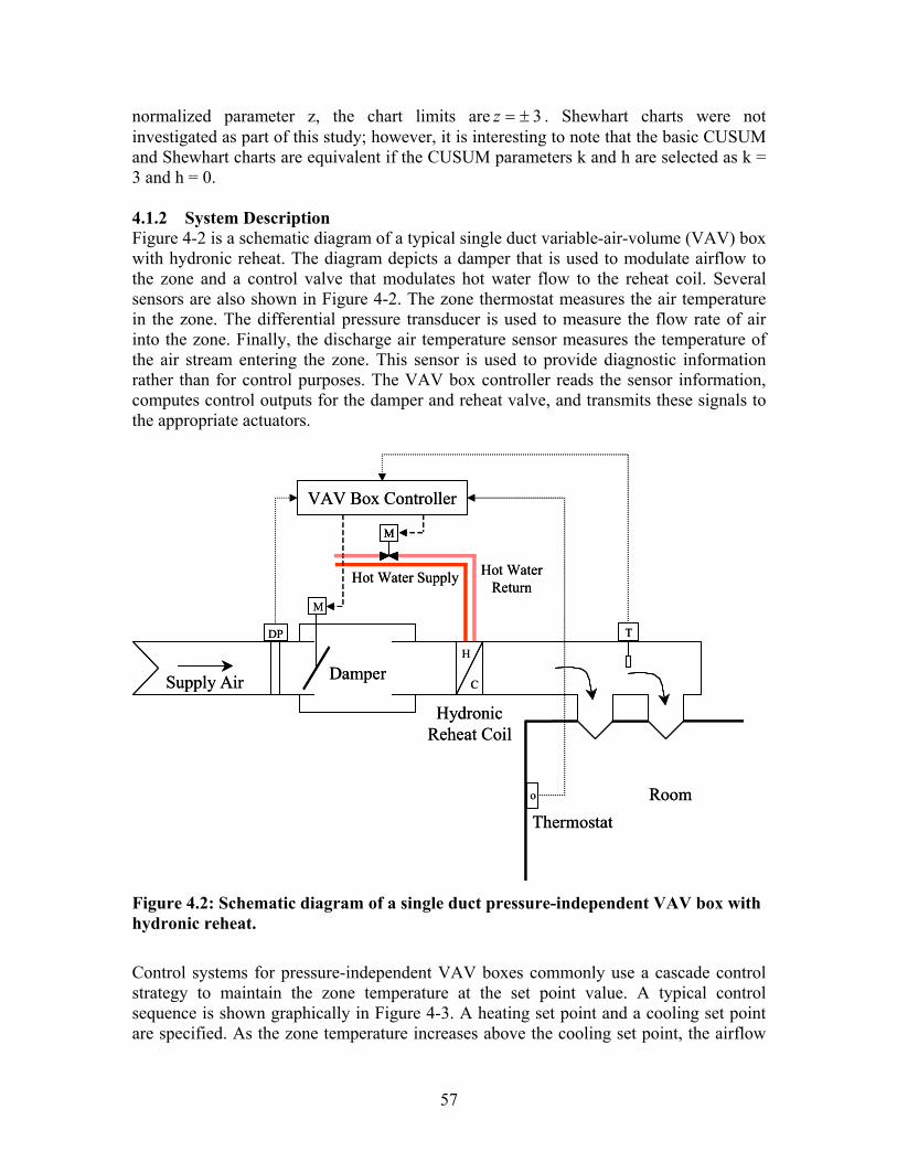
normalized parameter z, the chart limits are 3 ±=z . Shewhart charts were not investigated as part of this study; however, it is interesting to note that the basic CUSUM and Shewhart charts are equivalent if the CUSUM parameters k and h are selected as k = 3 and h = 0.

Coil

o

Hot Water Return

Coil

o

Hot Water Return

4.1.2 System Description Figure 4-2 is a schematic diagram of a typical single duct variable-air-volume (VAV) box with hydronic reheat. The diagram depicts a damper that is used to modulate airflow to the zone and a control valve that modulates hot water flow to the reheat coil. Several sensors are also shown in Figure 4-2. The zone thermostat measures the air temperature in the zone. The differential pressure transducer is used to measure the flow rate of air into the zone. Finally, the discharge air temperature sensor measures the temperature of the air stream entering the zone. This sensor is used to provide diagnostic information rather than for control purposes. The VAV box controller reads the sensor information, computes control outputs for the damper and reheat valve, and transmits these signals to the appropriate actuators.

Room

H

C

DP

HydronicReheat

VAV Box Controller

Thermostat

T

Damper

Hot Water Supply

M

M

Supply Air

Room

H

C

DP

HydronicReheat

VAV Box Controller

Thermostat

T

Damper

Hot Water Supply

MM

M

Supply Air

Figure 4.2: Schematic diagram of a single duct pressure-independent VAV box with hydronic reheat. Control systems for pressure-independent VAV boxes commonly use a cascade control strategy to maintain the zone temperature at the set point value. A typical control sequence is shown graphically in Figure 4-3. A heating set point and a cooling set point are specified. As the zone temperature increases above the cooling set point, the airflow

57

rate to the zone increases proportionally. This is accomplished by resetting the setpoint value of the airflow rate and modulating the damper to achieve this flow rate. As the zone temperature decreases below the cooling set point, the damper gradually decreases until it is providing the minimum flow rate necessary for ventilation. If the room temperature continues to decrease and reaches the heating set point, the reheat valve will begin to open. The airflow rate can also be varied in the heating mode, with the airflow increasing as the temperature decreases. Alternatively, a higher fixed airflow rate may be specified for heating operation to improve the distribution of the warm air. In Figure 4-3, it is assumed that a fixed airflow rate associated with the ventilation requirement of the room is provided in the heating mode.

igure 4.3: Damper and valve control sequence as a function of room temperature

1.3 CUSUM Applied to VAV Box Diagnostics box control strategy. However, a

from its value during normal operation, which can be detected by a CUSUM chart.

Airflow Setpoint

HeatingSet

Point

CoolingSet

Point

Room Temperature

Valve Position

MaximumFully Open

Fully Closed

Airflow Setpoint

Valve

HeatingSet

Point

CoolingSet

Point

Room Temperature

Valve Position

Minimum

Fully Open

Fully Closed

Valve

Ffor a single duct pressure-independent VAV box with hydronic reheat. 4.The previous section described one particular VAVwide variety of control strategies are employed by controller manufacturers, most of which use a cascaded control loop to maintain the zone temperature and zone airflow rate at setpoint values. In order to make VPACC independent of the control strategy used in a particular controller/VAV box application, three generic errors were identified: the airflow rate error, the temperature error, and the reheat coil differential temperature error. As long as the VAV box controller has an airflow setpoint, as well as heating and cooling temperature setpoints, VPACC will function independently of the control strategy used. Each fault considered in this study will result in a deviation of one or more of these errors

58

The airflow rate error, Qerror, is defined as

Qerror = Qactual - Qsetpoint Qactual is the actua point is the airflow rate setpoint. The CUSUM of

is error will detect stuck damper faults, differential pressure sensor faults, and unstable

e error, Temperror, is defined as

If Temproom > CSP Temperror = 0 : If HSP <

l airflow rate and Qsetthairflow faults. The temperatur

Temperror = Temproom – CSP : Temproom < CSP

Temproom is the ro cooling setpoint, and HSP is the heating

tpoint. The CUSUM of the temperature error will detect damper faults, valve faults,

erature error, ∆Terror, is defined as

∆Terror = 0 : If uhc ≠ 0 DAT is the discha erature (the temperature of the air leaving the reheat coil),

AT is the entering air temperature (the temperature of the air entering the reheat coil),

ulated during occupied periods. During noccupied periods, the errors are not computed, and the CUSUMs are reset to zero. The

ost of the points required by VPACC are already available in the local VAV box cooling setpoint, heating setpoint, airflow rate setpoint,

Temperror = HSP - Temproom : If Temproom < HSP

om temperature, CSP is theseand temperature sensor faults. The specific definition of temperature error used in this report is based on the control sequence described above. Various other commonly used control sequences may require changes to the definitions of heating setpoint, cooling setpoint, and temperature error. The reheat coil differential temp

∆Terror = DAT – EAT : If uhc = 0

rge air tempEand uhc is the control signal to the reheat coil valve. The CUSUM of the reheat coil differential temperature error will detect a leaking valve fault. Although this error is only used to detect one fault, this is a fault that highlights the advantages of automated FDD. Without VPACC, the local controller masks this fault from the occupants by increasing the airflow rate into the space. There will be no “too hot” or “too cold” complaints, so a significant energy penalty may be accrued. The errors and CUSUMs are only calcufirst hour of the occupied period is treated the same as the unoccupied period, to allow steady state conditions to develop. 4.1.4 Point requirements Mcontroller: room temperature, actual airflow rate, and occupancy status. Entering air temperature is typically not available, so supply air temperature (available over the control network from the AHU controller) could be used. Many VAV boxes are equipped with a discharge air temperature sensor, which VPACC needs in order to calculate the reheat coil differential

59

temperature error. If a discharge air temperature sensor is not available, a simplified version of VPACC could be used, implementing the airflow rate error and the temperature error only. In this case, a leaking reheat coil valve would not be detected. 4.1.5 Threshold Selection Two different sets of thresholds are used in the CUSUM method. Each of the three errors

as a slack parameter associated with it, which serves to filter out the variation of that

AV box pes, sizes, and control strategies. Data taken during normal operation will be used to

Accuracy Requirements PACC uses existing points in the building automation system to perform all

lready installed for control purposes

he ERS has two test VAV air-handling systems, referred to as AHU-A and AHU-B, l of that found in commercial

ets include normal operation data and data for three faults, namely, a failed ifferential pressure sensor, a hydronic reheat coil valve stuck partially open, and an

essure Sensor his fault was introduced during an unoccupied period by disconnecting both tubing

fault is expected to cause the VAV box

herror during normal operation. In addition, the S (positive) and T (negative) cumulative sums of each error have alarm limits, which identify when a fault has occurred. In order to determine threshold values, data must be collected for a variety of Vtydetermine slack parameters, and data for operation with various faults will be used to determine alarm limits. 4.1.6 InstrumentationVcalculations. The industrial grade sensors that are ahave sufficient accuracy. Laboratory grade instruments are not required. 4.2 Results from VAV Box Laboratory Experiments Teach serving four zones. The HVAC equipment is typicabuildings. The VAV boxes are single duct throttling units having both hydronic and electric reheat capabilities. They were operated with hydronic reheat to produce the current data sets. The VAV boxes are well instrumented; many more points are monitored than would commonly be available in a commercial building. During testing the HVAC equipment was operated in an occupied mode from 8:00 am to 5:00 pm and unoccupied otherwise. For normal operation, the AHU supply air temperature is 12.8 ºC (55 ºF) and the static pressure is 300 Pa (1.2 in w.g.). Data were collected at 1 min intervals. The data sdunstable control loop. The procedure for implementing the faults and their expected impacts are described below. 4.2.1 Faults Implemented 4.2.1.1 Failed Differential PrTleads to the differential pressure sensor. The damper to go to the full open position because the flow sensor will indicate an airflow rate of zero and the PI loop will attempt to correct for this condition.

60

4.2.1.2 Hydronic Reheat Coil Valve Stuck Partially Open This fault was implemented by applying a control voltage from an independent source to

e hydronic coil valve actuator. The severity of the fault was adjusted periodically to 0.1 GPM) to 0.00003 m3/s

Water Entering Leaving

Airflow Entering Air rature ))

Leaving Air Temperature ( ºC (ºF))

thproduce flow rates through the coil varying from 0.0063 m3/s ((0.5 GPM). The fault causes the discharge air temperature to be significantly higher than the entering air temperature for control conditions that indicate the reheat valve is closed. The impact of the fault was quantified by providing a fixed airflow rate to the VAV box and measuring the air temperature rise across the reheat coil. The data are summarized in Table 4.1.

Table 4.1: Hydronic Reheat Coil Valve Stuck Partially Open

Leakage Rate

Water Temperature

Water Temperature

Rate (m3/s

Tempe( ºC (ºF

(m3/s (GPM))

( ºC (ºF)) ( ºC (ºF)) (CFM)) *

7.6 10x -6 ) ) (0.12)

57.4 (135.3) 32.8 (91.1) 0.28 (598)

13.9 (57.1 16.0 (60.8

1.5x10-5 (0.23)

57.8 (136.0) 33.5 (92.3) 8

14.3 (57.8) 18.2 (64.8) 0.2(602)

2.1x10-5 57.7 (135.8) 36.1 (97.0)

13.2 (55.8) 18.4 (65.1) (0.34)

0.28 (599)

2.8x10-5 58.0 (136.4) 38.8 (101.8)

12.6 (54.6) 18.5 (65.3) (0.45)

0.29 (605)

3.4x10-5 58.7 (137.6) 41.0 (105.8)

12.9 (55.3) 19.6 (67.2) (0.54)

0.29 (604)

3/s (600 CFM as establishrflow p

*A fixed supply airflow rate of approximately 0.28 m ) w ed by setting the minimum and the maximum ai arameters for the VAV box to 0.28

3/s (600 CFM).

4.2Th ented by changing the integral coefficient of the controller used for airflow control. The parameter referred to as the “reset action” by the manufacturer was

0.5 to 15.0. The fault caused the VAV box damper to

rgy Center (IEC). The first set is ormal operation only. The second set is a combination of normal and faulty operation.

e

m .1.3 Unstable Control Loop e fault was implem

adjusted from the normal value ofcycle continuously with a cycling period of approximately 2 min and 15 s. The impact should be similar to that of unstable static pressure control for the supply fan, although the impact should be localized to a single VAV box. 4.2.2 Normal Operation Two sets of data were collected from the Iowa Enen Normal operation data were collected from four VAV box controllers once per minute during the occupied periods of eight different days. The airflow rate error, th

61

temperature error, and the reheat coil differential temperature error were calculated for

or Mean Standard Deviation

each one-minute sample. The mean and standard deviation were calculated for each error.

Table 4.2: Error Statistics For Normal Operation.

ErrQerror 0 m /s (0 CFM) 3 0.002 m3/s (5 CFM) Temp 0.026 ºC (0.1 ºF) error 0.026 ºC (0.1 ºF) ∆Terror 0.044 ºC (0.8 ºF) 0.038 ºC (0.7 ºF)

ed faults were use e CUSUM charts

4.2.3 Control Charts Data collected from the implement d to creat of the irflow rate error, the temperature error, and the reheat coil differential temperature error.

using Equation 1 and the mean and standard deviation values

on e room cause the room temperature to increase. The controller responds by increasing

value of Qactual is zero. This VAV box has a inimum Qsetpoint of 0.09 m3/s (200 CFM) (to meet ventilation requirements). The PI

aThe errors were normalizedfrom the “normal operation” data collected previously. The slack parameter k in Equations 2 and 3 was set equal to a value of 3. Plots showing various operating parameters, followed by the CUSUM charts for each zone were generated for each date data was collected. Detailed results are presented for one day of typical normal operation (no faults) in one VAV box and one day of operation with a failed differential pressure sensor in one VAV box, followed by a summary of all VPACC results from the ERS. Figure 4.4 shows the results for one day of normal operation (no faults) from a single VAV box. When the occupied period begins, the internal and external cooling loadsthQsetpoint. The damper is modulated to maintain the Qactual close to the Qsetpoint. Since the room temperature is above the HSP the reheat coil valve stays closed. (Note that the damper is closed when the control signal is 0 %, the reheat coil valve is closed when the control signal is 100 %). As a result, the Qerror is very small and the Qerror CUSUM is negligible as well. The control algorithm maintains room temperature close to the cooling setpoint, so the Temperror and Temperror CUSUM are also negligible. There is a small difference between entering air temperature and discharge air temperature due to measurement errors from the temperature sensors. The use of the slack parameter results in zero values for the ∆Terror CUSUM. Figure 4.5 shows results for one day of operation with a failed differential pressure sensor. As expected, the measured malgorithm used to determine damper position quickly saturates at full open due to the Qerror of 0.09 m3/s (200 CFM). The Qerror CUSUM steadily increases, ending up with a value of 20 000 by the end of the occupied period. The fully open damper causes the room temperature to fall below the heating setpoint. At this point, the controller opens the reheat valve, which brings the room temperature back up to the heating setpoint. At first, the Temperror and Temperror CUSUM register the effect of dropping room temperature. As the reheat valve regains control of the room temperature, the Temperror and Temperror CUSUM decrease to normal levels. By midday, is enough of a cooling load to maintain the room temperature above the HSP without reheat. As the reheat valve

62

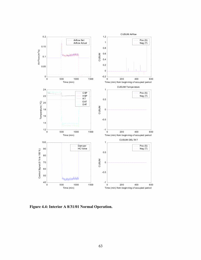
0 500 1000 15000

0.05

0.1

0.15

0.2

Time (min)

Air

Flow

(m3 /s

)Airflow SetAirflow Actual

0 200 400 600-0.2

0

0.2

0.4

0.6

0.8

1

1.2CUSUM: Airflow

Time (min) from beginning of occupied period

CUS

UM

Pos (S)Neg (T)

0 500 1000 150012

14

16

18

20

22

24

Time (min)

Tem

pera

ture

(o C

)

CSPHSPRTEATDAT

0 200 400 600-1

-0.5

0

0.5

1CUSUM: Temperature

Time (min) from beginning of occupied period

CUS

UM

Pos (S)Neg (T)

0 500 1000 150040

50

60

70

80

90

100

Time (min)

Con

trol S

igna

l (0

% to

100

%)

Dam perHC Valve

0 200 400 600-1

-0.5

0

0.5

1CUSUM: DELTA T

Time (min) from beginning of occupied period

CUS

UM

Pos (S)Neg (T)

Figure 4.4: Interior A 8/31/01 Normal Operation.

63

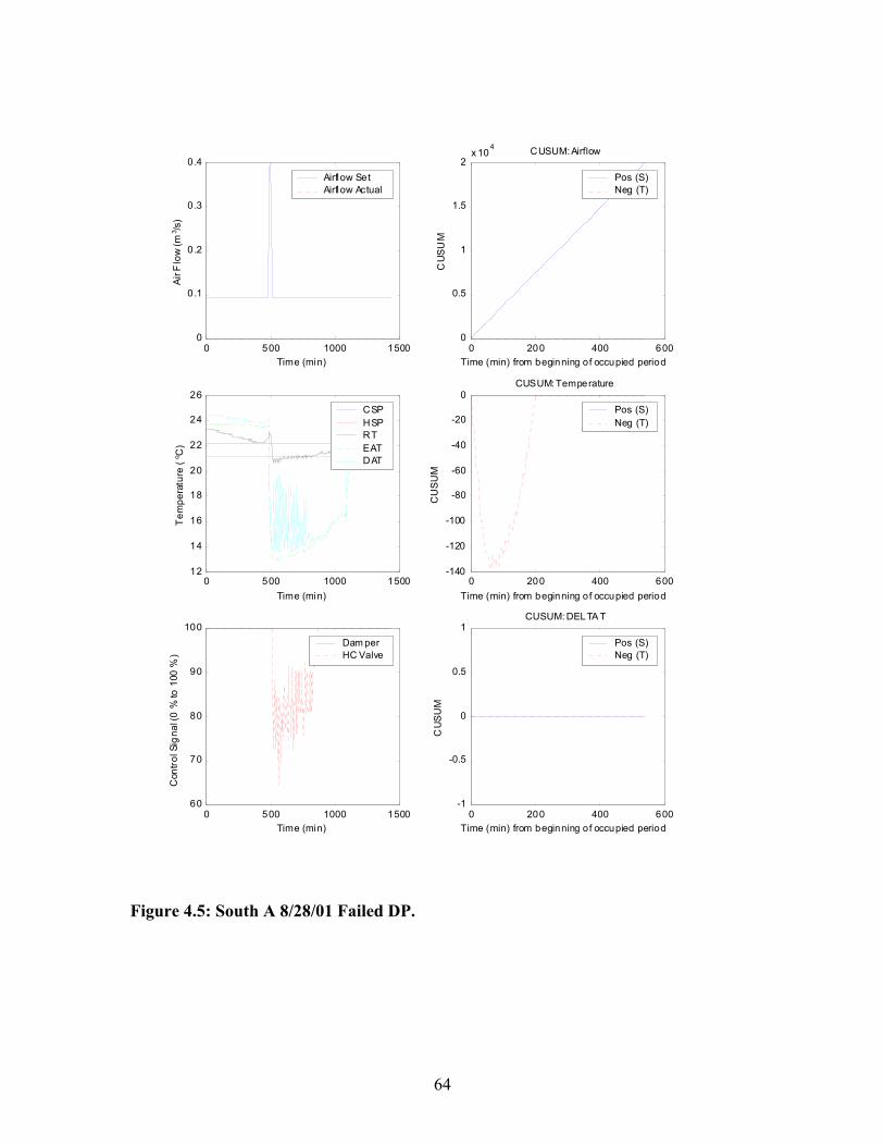
0 500 1000 15000

0.1

0.2

0.3

0.4

Time (min)

Air F

low

(m3 /s

)Airflow SetAirflow Actual

0 200 400 6000

0.5

1

1.5

2x 10

4 CUSUM: Airflow

Time (min) from beginning of occupied period

CUS

UM

Pos (S)Neg (T)

0 500 1000 150012

14

16

18

20

22

24

26

Time (min)

Tem

pera

ture

(o C

)

CSPHSPRTEATDAT

0 200 400 600-140

-120

-100

-80

-60

-40

-20

0CUSUM: Temperature

Time (min) from beginning of occupied period

CU

SUM

Pos (S)Neg (T)

0 500 1000 150060

70

80

90

100

Time (min)

Con

trol S

igna

l (0

% to

100

%)

Dam perHC Valve

0 200 400 600-1

-0.5

0

0.5

1CUSUM: DELTA T

Time (min) from beginning of occupied period

CUS

UM

Pos (S)Neg (T)

Figure 4.5: South A 8/28/01 Failed DP.

64

modulates in response to room temperature, the discharge air temperature increases and decreases accordingly. Since the control signal to the reheat valve is not “full close”, the ∆Terror and ∆Terror CUSUM are reset to zero. Table 4.3 shows a range of values for alarm limits for each CUSUM indicated. These values will detect all of the faults in the data set without any false alarms. As long as the alarm limit for each S and T function is set between the minimum and maximum limits, every fault will be detected with zero false alarms. “Not used” indicates that the limit was not needed to detect any of the particular faults that were implemented, although the limit may be needed to detect other faults. These preliminary results do not constitute a rigorous statistical approach. Before definitive alarm limits can be established, much additional data needs to be collected across a range of VAV box types, cooling/heating/swing seasons, size ranges, and controller manufacturers. It may be necessary to adjust the alarm limits based on one or more of these parameters. For example, there might be a set of alarm limits for small VAV boxes, another for medium boxes, and another for large boxes.

Table 4.3: Alarm Limits

Minimum Alarm Limit Maximum Alarm Limit Airflow positive (S) 3 180 Airflow negative (T) 3 100 Temperature positive (S) 120 950 Temperature negative (T) 0 Not used DELTA T positive (S) 0 400 DELTA T negative (T) 0 Not used Table 4.4 shows the peak values of each CUSUM chart for each run. The bold values show where each CUSUM identified exceeds the alarm limits from Table 4.3, detecting a fault. 4.3 Results from VAV Box Simulation Using HVACSIM+ Simulation, as described in the introduction of this report, was used to test and refine VPACC. The simulation consisted of a single floor in a commercial office building with a VAV AHU and three VAV boxes. The VAV boxes are modeled as single duct, throttling units with hydronic reheat coils. In order to leverage previous VAV box modeling work, a pressure dependent system was used (the VAV box damper is positioned directly as a function of zone temperature, there is no airflow rate sensor or airflow rate setpoint). Although this type of system no longer represents a typical installation in the industry, its use here illustrates the flexibility, as well as some of the

s other than the pressure independent system described in 4.1.2.

limitations, of adapting VPACC to system

65

Table 4.4: CUSUM Chart Peak Values

Date Zone Fault S T S T S T /30/01 East A Normal Operation 1

CFM CFM TEMP TEMP ∆T ∆T8 -1 100 0 0 0 8/31/01 East A Normal Operation 3 -3 30 0 0 0 9/1/01 East A Normal Operation 2 -2 0.6 0 0 0 8/28/01 Interior A Normal Operation 0 0 120 0 0 0 8/30/01 Interior A Normal Operation 0.5 0 0 0 0 0 8/31/01 Interior A Normal Operation 1 0 0 0 0 0 9/1/01 Interior A Normal Operation 0 0 0 0 0 0 8/28/01 South A Failed DP 20 000 0 0 -120 0 0 8/30/01 South A Failed DP 20 000 0 0 -150 0 0 8/31/01 South A Unstable Airflow 200 -25 200 0 0 0 9/1/01 South A Unstable Airflow 30 -100 0 0 0 0 8/28/01 West A Stuck HC Valve 180 0 950 0 400 0 8/30/01 West A Stuck HC Valve 8 -1 9 0 2400 0 8/31/01 West A Stuck HC Valve 10 -5 9 0 4000 0 9/1/01 West A Normal Operation 3 -1 0 0 0 0 4.3.1 Faults Implemented

amper S k Open by g the VAV box damper actuator position to the full

irf the maximum, and zone temperature will ooling load is small enough, the zone erature will drop below using t hydronic reheat valve to op mpt to maintain

one temperature at the setpoint.

ault was introduced by setting the VAV box damper actuator to the minimum osition. The zone airflow will go to the minimum value, and zone temperature will tend

ill not be seen when the

Hydronic Reheat Coil Valve Stuck Closed his fault was introduced by setting the VAV box hydronic reheat coil valve actuator osition to zero. If there is a heating load, the fault is expected to cause the zone mperature to drop.

4.3.1.1 VAV Box D tucThis fault was introduced settinopen position. The zone a low will go to decrease. If the zone c tempthe heating setpoint, ca he en in an attez 4.3.1.2 VAV Box Damper Stuck Closed This fpto increase for cooling conditions. The impact of the fault wVAV box operates in the heating mode because, according to the simulated control strategy, the damper will already be set to the minimum position. 4.3.1.3 VAV Box Hydronic Reheat Coil Valve Stuck Open This fault was introduced by setting the VAV box hydronic reheat coil valve actuator position to full open. The zone temperature is expected to rise above the cooling setpoint, causing the damper actuator to open in an attempt to maintain zone temperature at the set point. 4.3.1.4 VAV Box Tpte

66

4.3.2 Normal Operation The simu ny season. Th int n co in loads the

se e z g th a o g mo fully greater th ini fo e ent occupied g of t only rence between one season and

to V u of the cooling load in each of the zones. f e esented in this section. Two weeks of n g f or “n mal operation” case, and for each u c m at coi fferen l

tu e a ute d a poi The ean and d we d for eac e st stical parameters of these r ed rom the Io r Cent s me th da re to nerate e control 4 o t ria s inh n ulation.

o arle t ault ere u to c te C UM c f e

tu and fferential t erature erro The ors were ormalized using Equation 1 and the mean and standard deviation values from the

ed from the ERS. The slack parameter k in Equations 2 nd 3 was set equal to a value of 3.

the proportional control algorithm combine to produce damper control signal that closely mirrors the zone temperature. This control algorithm

cooling setpoint, so the Temperror and the

igure 4.7 shows the results for one day of the reheat coil valve stuck open fault (fault is fully open, the zone

The ∆Terror CUSUM also increases to a value of 10 000 by the end of the ccupied period, because the reheat coil valve control signal is zero, and there is a

eratures. The Temperror

lation can use weather data from a e er al ol g model u s for th ones are large enou h that e VAV box

)es re in c olin ode

(reheat cre

il valve closed, airflow rate an m mum r th ireperiod another

ardless the VA

the season, so thatboxes is the magnit

he de

diffe

Results rom one season only, fall, ar prsimulatio data were enerated for the no ault, orof the fo r faults des ribed above. The te perature error and the rehe l di tiatempera re error w re calculated for e ch one-min at nt. mstandard eviation re calculate h error. Th atierrors we e compar to results f wa Ene gy er (IEC) as described in 4.2. The stati tical para ters calculated for e IEC ta we used ge thcharts in .3.3 due t he small process va tion erent i sim 4.3.3 C ntrol Ch ts Data col cted from he implemented f s w sed rea US harts o thtempera re error the reheat coil di emp r. errn“normal operation” data collecta Figure 4.6 shows the results for one day of normal operation (no faults) from the three VAV boxes in the simulation. When the occupied period begins, the internal and external cooling loads on the room cause the room temperature to increase. The controller responds by increasing the damper control signal. The combination of a pressure dependent VAV box andamaintains room temperature close to the associated CUSUM statistics are negligible. There is a small difference between entering air temperature and discharge air temperature due to heat gain in the supply ducts and the thermal mass effects of the reheat coil. The use of the slack parameter results in zero values for the ∆Terror CUSUM. Fimplemented in zone 1 only). Since the reheat coil valve temperature rises well above the cooling setpoint. The airflow control signal is increased to 100 % in response to the room temperature. As shown in Figure 4.8, the Temperror CUSUM steadily increases, ending up with a value of 20 000 by the end of the occupied period.odifference between the VAV box entering and discharge air tempand ∆Terror CUSUMs are reset to zero during each unoccupied period.

67

0.6 (m

0.4

Ctrl

Sig

n

0.8

1 Z2 udZ2 uhc

0.2

A 0.2

0.4

Ctrl

S

1.1 1.2 1.3 1.4 1.5 1.6

x 105

15

20

25

30

Time (s )

Tem

pera

ture

(o C

)CSPHSPZone 1Zone 2Zone 3

1.1 1.2 1.3 1.4 1.5 1.6

x 105

0

10

20

30

40

50

Time (s)

Tem

pera

ture

(o C

)

SATDAT Z1DAT Z2DAT Z3

0.8

1

3 /s)

Z1

0.6

0.8

1

al

Z1 udZ1 uhc

1.1 1.2 1.3 1.4 1.5 1.6

x 105

0

0.2

Time (s )

Ai

1.1 1.2 1.3 1.4 1.5 1.6

x 105

0

0.2

Time (s)

1 Z2

0.4rflow

1.1 1.2 1.3 1.4 1.5 1.6

x 105

0

0.2

0.4

0.6

0.8

Time (s )

Airfl

ow (m

3 /s)

1.1 1.2 1.3 1.4 1.5 1.6

x 105

0

0.2

0.4

0.6

Time (s)

Ctrl

Sig

nal

0 .4

0.6

0.8

1

irflo

w (m

3 /s)

Z3

0.6

0.8

1

igna

l

Z3 udZ3 uhc

1.1 1.2 1.3 1.4 1.5 1.6

x 105

0

Time (s )1.1 1.2 1.3 1.4 1.5 1.6

x 105

0

Time (s)

Figure 4.6 Simulation - normal operation - process variables and control signals

68

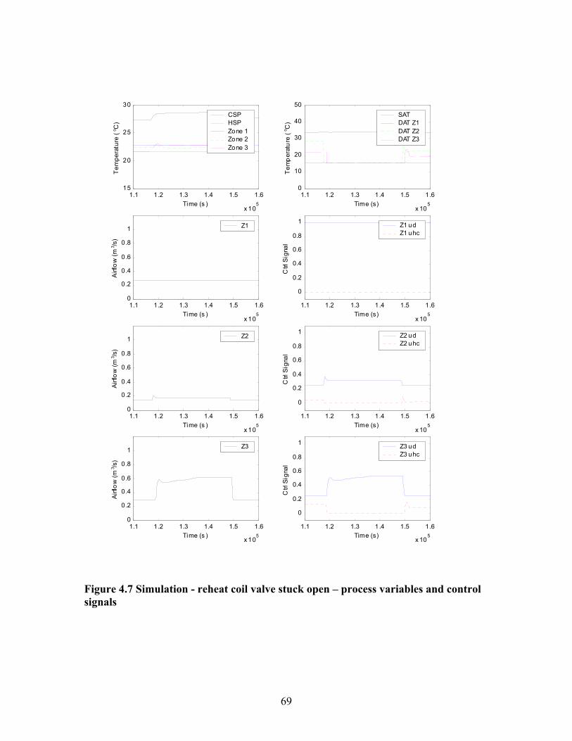
1.1 1.2 1.3 1.4 1.5 1.6

x 105

15

20

25

30

Time (s )

Tem

pera

ture

(o C

)CSPHSPZone 1Zone 2Zone 3

1.1 1.2 1.3 1.4 1.5 1.6

x 105

0

10

20

30

40

50

Time (s)

Tem

pera

ture

(o C

)

SATDAT Z1DAT Z2DAT Z3

1.1 1.2 1.3 1.4 1.5 1.6

x 105

0

0.2

0.4

0.6

0.8

1

Time (s )

Airfl

ow (m

3 /s)

Z1

1.1 1.2 1.3 1.4 1.5 1.6

x 105

0

0.2

0.4

0.6

0.8

1

Time (s)

Ctrl

Sig

nal

Z1 udZ1 uhc

1.1 1.2 1.3 1.4 1.5 1.6

x 105

0

0.2

0.4

0.6

0.8

1

Time (s )

Airfl

ow (m

3 /s)

Z2

1.1 1.2 1.3 1.4 1.5 1.6

x 105

0

0.2

0.4

0.6

0.8

1

Time (s)

Ctrl

Sig

nal

Z2 udZ2 uhc

1.1 1.2 1.3 1.4 1.5 1.6

x 105

0

0.2

0.4

0.6

0.8

1

Time (s )

Airfl

ow (m

3 /s)

Z3

1.1 1.2 1.3 1.4 1.5 1.6

x 105

0

0.2

0.4

0.6

0.8

1

Time (s)

Ctrl

Sig

nal

Z3 udZ3 uhc

Figure 4.7 Simulation - reheat coil valve stuck open – process variables and control

gnals si

69

450 500 550 600 650 700 750 800 850 900-2.5

-2

-1 .5

-1

-0 .5

0

0.5

1

1.5

2

2.5x 10

4 CUSUM: Tem perature

Time (min)

CUS

UM

Zone 1Zone 2Zone 3

450 500 550 600 650 700 750 800 850 900-1.5

-1

-0 .5

0

0.5

1

1.5x 10

4 CUSUM: DELTA T

Time (min)

CUS

UM

Zone 1Zone 2Zone 3

Figure 4.8 Simulation - reheat coil valve stuck open - CUSUM charts

70

Table 4.5 shows a range of values for alarm limits for each CUSUM indicated. These values will detect all of the faults in the data set (that can be detected) without any false alarms.

Table 4.5: Alarm Limits

Minimum Alarm Limit Maximum Alarm Limit Temperature positive (S) 0 4000 Temperature negative (T) 0 Not used DELTA T positive (S) 0 10 000 DELTA T negative (T) 0 Not used As long as the alarm limit for each S and T function is set between the minimum and maximum limits, every fault that can be detected will be detected with zero false alarms. “Not used” indicates that the limit was not needed to detect any of the particular faults that were implemented, although the limit may be needed to detect other faults. These preliminary results do not constitute a rigorous statistical approach. Before definitive alarm limits can be established, much additional data needs to be collected across a range of VAV box types, cooling/heating/swing seasons, size ranges, and controller manufacturers. It may be necessary to adjust the alarm limits based on one or more of these parameters. For example, there might be a set of alarm limits for small VAV boxes, another for medium boxes, and another for large boxes. In order to leverage work done previously by NIST [4], this study used a model that was originally written primarily to develop FDD tools for air handling units. Some limitations of this model regarding its use as a zone/VAV box simulator have become apparent. The first limitation was mentioned earlier: the internal loads for each zone are so great relative to the shell loads that all seasons are qualitatively the same. Each zone is in cooling mode for the entire occupied period. For this reason, the reheat coil valve stuck closed fault is not detected by the CUSUM method, since it has no impact on system operation during cooling mode. Another limitation is that the VAV boxes are modeled as pressure dependent boxes, meaning the damper is controlled directly in response to zone temperature without an intermediate determination of an airflow setpoint. A Qerror does not exist for a pressure dependent VAV box. The damper stuck open fault is a fault which is masked by the controls. As the zone cools below the heating setpoint, the reheat coil valve opens to provide heating to the zone. Without a Qerror CUSUM, this fault cannot be detected. Table 4.6 shows the peak values of each CUSUM chart for each run. The bold values show where each CUSUM identified exceeds the alarm limits from Table 4.5, detecting a fault.

.4 Results from VAV Box Emulation in the VCBT Emulation, using the VCBT as described in the introduction of this report, was used in addition to simulation, to test and refine VPACC. The emulation consisted of a commercial office building with a VAV AHU and three VAV boxes for each floor. The VAV boxes were modeled as single duct, throttling units with hydronic reheat coils. On

4

71

one of the floors, one manufacturer’s commercially available zone controllers were used to implement a pressure dependent control strategy as described in 4.3. On another floor, a different manufacturer’s commercially available zone controllers were used to

endent control strategy as described in 4.1.2.

t Pe Values

STEMP TTEM T∆T

implement a pressure indep

Table 4.6: CUSUM Char ak

Fault P ∆T S Normal operation 0 0 0 0Damper stuck fully open 0 0 0 0 Damper stuck fully closed 4000 0 0 0 Reheat coil valve stuck fully open 20 000 0 10 000 0 Reheat coil valve stuck fully closed 0 0 0 0

4.4.1 Faults Implemented The faults implemented in the emulation are essentially the same as those considered in the simulation with the exception of a few details. The description below was included to illustrate those exceptions, as well as in the interest of completeness and to enable each section to stand alone to the extent possible. 4.4.1.1 VAV Box Damper Stuck Open

alve Stuck Open his fault was introduced by setting the VAV box hydronic reheat coil valve actuator

mperature at the set point.

losed

This fault was introduced by setting the VAV box damper actuator position to the full open position. The zone airflow will go to the maximum, and zone temperature will decrease. If the zone cooling load is small enough, the zone temperature will drop below the heating setpoint, causing the hydronic reheat valve to open in an attempt to maintain zone temperature at the setpoint. 4.4.1.2 VAV Box Damper Stuck Closed This fault was introduced by setting the VAV box damper actuator to the minimum position. The zone airflow will go to the minimum value, and zone temperature will tend to increase for cooling conditions. The impact of the fault will not be seen when the VAV box operates in the heating mode because the reheat coil valve will still modulate to heat the air supplied to the zone, thereby controlling the zone temperature. 4.4.1.3 VAV Box Hydronic Reheat Coil VTposition to full open. The zone temperature is expected to rise above the cooling setpoint, causing the damper actuator to open, and airflow to increase, in an attempt to maintain zone te 4.4.1.4 VAV Box Hydronic Reheat Coil Valve Stuck CThis fault was introduced by setting the VAV box hydronic reheat coil valve actuator position to zero. If there is a heating load, the fault is expected to cause the zone temperature to drop. Under cooling conditions, this fault has no impact on system operation.

72

4.4.2 Normal Operation The emulation was run using weather data for “heating season” (winter), “swing season” (fall), and “cooling season” (summer). One week of fault free emulation data was generated for each of the seasons. The airflow error (pressure independent VAV boxes

nly), temperature error, and the reheat coil differential temperature error were calculated r each one-minute data point. An aggregate mean and standard deviation were

t-case results for the three seasons considered, the values shown in Table 4.7 were used as parame rs the M me o .

Table 4.7: Error Statistics For Normal Operation

Mean Standard

ofocalculated for each error. Based on wors

te for CUSU th d

.

Deviation e Independent

Rate Error /s MPressurAirflow 0 m3 (0 CF ) 0.02 m3/s (40 CFM)Temperature Error 0.1 ºC (0.2 ºF) 0.1 ºC (0.2 ºF) Reheat Coil Differential Temperature Error 0.0 ºC (0.0 ºF) 1.1 ºC (2.0 ºF) Pressure Dependent Temperature Error 0.0 ºC (0.0 ºF) 0.4 ºC (0.7 ºF) Reheat Coil Differential Temperature Error -1.1 ºC (-2.0 ºF) 1.4 ºC (2.5 ºF) 4.4.3 Control Charts A subset of the data collected from the emulation is presented here for illustrative purposes. The faults described in 5.4.1 were implemented in the following seasons: VAV box damper stuck open – heating season and swing season, VAV box damper stuck closed – swing season, VAV box hydronic reheat coil valve stuck open – swing season and cooling season, VAV box hydronic reheat coil valve stuck closed – heating season.

ne to two days of data were generated for each fault. Data collected from the M charts of the temperature error and the

e heating load decreases, the room temperature rises. decreasing the airflow

e internal and external

erroraintains room temperature close to the cooling setpoint, so the Temperror is

Oimplemented faults were used to create CUSUreheat coil differential temperature error. The errors were normalized using Equation 1 and the mean and standard deviation values from the “normal operation” data collected previously. The slack parameter k in Equations 2 and 3 was set equal to a value of 3. Plots showing various operating parameters are followed by the CUSUM charts for three zones on each date data were collected. Figure 4.9 shows the results for one day of heating season normal operation (no faults) from the three VAV boxes in the pressure independent part of the emulation. When the occupied period begins (120 min into the emulation), the room temperatures are below the heating setpoint, so the reheat coil valves open and the airflow rates increase. As the ontrol actions take effect and thc

The controllers respond by closing the reheat coil valves andsetpoint and airflow for each room. As the day progresses thcooling loads increase. The controllers respond by increasing the airflow setpoint and airflow for each room. The airflow control loop in the zone controller maintains the airflow rate close to the airflow setpoint, so the Q is negligible. This control algorithm m

73

also negligible. There is little difference between entering air temperature and discharge

nd the eating load decreases, the room temperature rises. The controllers respond by closing

ternal and external cooling loads eratures increase above the cooling

tpoint and the controllers respond by increasing the damper positionre small, so the room temperatures remain below the cooling

per control signals remain valu room temperatures throughout the day. This thm

tin he Tem here is little difference between entering air temperature and discharge air temperature,

egligible. Consequently e CUSUM statistics are maintained well holds.

igure 4.11 shows one day of data from the swing season for the reheat coil valve stuck in the pressure independent VAV boxes (fault implemented in

re dependent VAV boxes (fault implemented in one 1 only). The behavior of zones 2 and 3 shows the same trends as in Figure 4.10 and

air temperature, so the ∆Terror is also negligible. Consequently the CUSUM statistics are maintained well below the fault thresholds. Figure 4.10 shows the results for one day of heating season normal operation (no faults) from the three VAV boxes in the pressure dependent part of the emulation. When the occupied period begins, the room temperatures are below the heating setpoint, so the reheat coil valves open as described in 4.3. As the control actions take effect ahthe reheat coil valves. As the day progresses the inincrease. If the loads are large enough, the room tempse of each VAV box. In this case, the loads a setpoint and the dam at their minimum es. The reheat coil valves maintain the control algorimaintains room temperature close to the hea g setpoint, so t perror is negligible. Tso the ∆Terror is also n thbelow the fault thres Fopen fault as implemented zone 1 only). The behavior of zones 2 and 3 shows the same trends as in Figure 4.9 and any differences are due to the different season. Since the reheat coil valve in zone 1 is fully open, the zone temperature rises well above the cooling setpoint. The airflow rate setpoint and airflow control signal are increased to their maximum values in response to the room temperature. Figure 4.12 shows that the Temperror CUSUM steadily increases, ending up with a value of 11 000 by the end of the occupied period of the day. The ∆Terror CUSUM also increases to a value of 2500 by the end of the occupied period of the day, because the reheat coil valve control signal is zero, and there is a difference between the VAV box entering and discharge air temperatures. Figure 4.13 shows one day of data from the swing season for the reheat coil valve stuck open fault as implemented in the pressuzany differences are due to the different season. Since the reheat coil valve in zone 1 is fully open, the zone temperature rises well above the cooling setpoint. The damper control signal is increased to 100 % in response to the room temperature. Figure 4.14 shows that the Temperror CUSUM steadily increases, ending up with a value of 2000 by the end of the occupied period of the day. The ∆Terror CUSUM also increases to a value of 2500 by the end of the occupied period of the day, because the reheat coil valve control signal is zero, and there is a difference between the VAV box entering and discharge air temperatures.

74

CSP50

SAT SP

600)

0 200 400 600Time (min)

0 .6

0.6 (m ign

30

0 200 400 60015

20

25

Time (min)

Tem

pera

ture

(o C

) HSPZ1Z2Z3

0 200 400 6000

10

20

30

40

Time (min)

Tem

pera

ture

(o C

) DAT Z1DAT Z2DAT Z3

0 200 4000

0.1

0.2

0.3

Time (min

Airfl

ow (m

3 /s)

Z1 AirflowZ1 Airflow SP

0

20

40

60

80

100

Ctrl

Sig

nal

Z1 udZ1 uhc

0 200 400 6000

0.2

0.4

Time (min)

Airfl

ow (m

3 /s)

Z2 AirflowZ2 Airflow SP

0 200 400 600

0

20

40

60

80

100

Time (min)

Ctrl

Sig

nal

Z2 udZ2 uhc

0.8

1

3 /s)

Z3 AirflowZ3 Airflow SP

60

80

100

al

Z3 udZ3 uhc

0 200 400 6000

0.2

0.4

Time (min)

Airfl

ow

0 200 400 600

0

20

40

Time (min)

Ctrl

S

Figure 4.9 Emulation – pressure independent - normal operation - process variables and control signals

75

0 200 400 60015

20

25

30

Time (min)

Tem

pera

ture

(o C

)CSPHSPZ1Z2Z3

0 200 400 6000

10

20

30

40

50

Time (min)

Tem

pera

ture

(o C

)

SATDAT Z1DAT Z2DAT Z3

0 200 400 6000

0.1

0.2

0.3

Time (min)

Airfl

ow (m

3 /s)

Z1

0 200 400 600

0

2

4

6

8

10

Time (min)

Ctrl

Sig

nal

Z1 udZ1 uhc

0 200 400 6000

0.2

0.4

0.6

Time (min)

Airfl

ow (m

3 /s)

Z2

0 200 400 600

0

2

4

6

8

10

Time (min)

Ctrl

Sig

nal

Z2 udZ2 uhc

0 200 400 6000

0.2

0.4

0.6

0.8

1

Time (min)

Airfl

ow (m

3 /s)

Z3

0 200 400 600

0

2

4

6

8

10

Time (min)

Ctrl

Sig

nal

Z3 udZ3 uhc

Figure 4.10 - Emulation – pressure dependent - normal operation - process variables and control signals

76

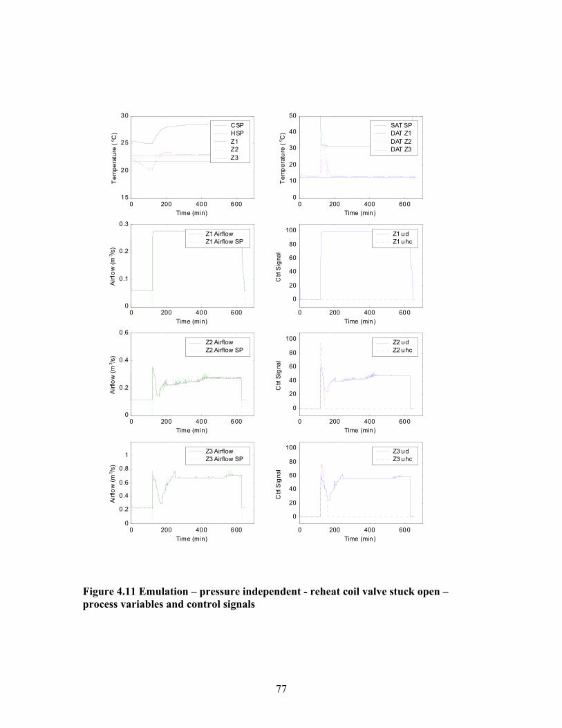
0 200 400 60015

20

25

30

Time (min)

Tem

pera

ture

(o C

)

CSPHSPZ1Z2Z3

0 200 400 6000

10

20

30

40

50

Time (min)

Tem

pera

ture

(o C

)

SAT SPDAT Z1DAT Z2DAT Z3

0 200 400 6000

0.1

0.2

0.3

Time (min)

Airfl

ow (m

3 /s)

Z1 AirflowZ1 Airflow SP

0 200 400 600

0

20

40

60

80

100

Time (min)

Ctrl

Sig

nal

Z1 udZ1 uhc

0 200 400 6000

0.2

0.4

0.6

Time (min)

Airfl

ow (m

3 /s)

Z2 AirflowZ2 Airflow SP

0 200 400 600

0

20

40

60

80

100

Time (min)

Ctrl

Sig

nal

Z2 udZ2 uhc

0 200 400 6000

0.2

0.4

0.6

0.8

1

Time (min)

Airfl

ow (m

3 /s)

Z3 AirflowZ3 Airflow SP

0 200 400 600

0

20

40

60

80

100

Time (min)

Ctrl

Sig

nal

Z3 udZ3 uhc

Figure 4.11 Emulation – pressure independent - reheat coil valve stuck open –

rocess variables and control signals p

77

0 50 100 150 200 250 300 350 400 450-6

-5

-4

-3

-2

-1

0

1CUSUM: Airflow

CUS

UM

Time (min) starting 1 h after beginning of occupied period

Zone 1Zone 2Zone 3

0 50 100 150 200 250 300 350 400 4500

2000

4000

6000

8000

10000

12000CUSUM: Tem perature

CU

SUM

Time (min) starting 1 h after beginning of occupied period

Zone 1Zone 2Zone 3

0 50 100 150 200 250 300 350 400 4500

500

1000

1500

2000

2500

3000CUSUM: DELTA T

CUS

UM

Time (min) starting 1 h after beginning of occupied period

Zone 1Zone 2Zone 3

Figure 4.12 Emulation – pressure independent - reheat coil valve stuck open -

ing of CUSUM charts (x axis shows elapsed time in minutes from 1 hour after beginnoccupancy)

78

0 200 400 60015

20

25

30

Time (min)

Tem

pera

ture

(o C

)CSPHSPZ1Z2Z3

0 200 400 6000

10

20

30

40

50

Time (min)

Tem

pera

ture

(o C

)

SATDAT Z1DAT Z2DAT Z3

0 200 400 6000

0.1

0.2

0.3

Time (min)

Airfl

ow (m

3 /s)

Z1

0 200 400 600

0

2

4

6

8

10

Time (min)

Ctrl

Sig

nal

Z1 udZ1 uhc

0 200 400 6000

0.2

0.4

0.6

Time (min)

Airfl

ow (m

3 /s)

Z2

0 200 400 600

0

2

4

6

8

10

Time (min)

Ctrl

Sig

nal

Z2 udZ2 uhc

0 200 400 6000

0.2

0.4

0.6

0.8

1

Time (min)

Airfl

ow (m

3 /s)

Z3

0 200 400 600

0

2

4

6

8

10

Time (min)

Ctrl

Sig

nal

Z3 udZ3 uhc

Figure 4.13 Emulation – pressure dependent - reheat coil valve stuck open – prvariables and control signals

ocess

79

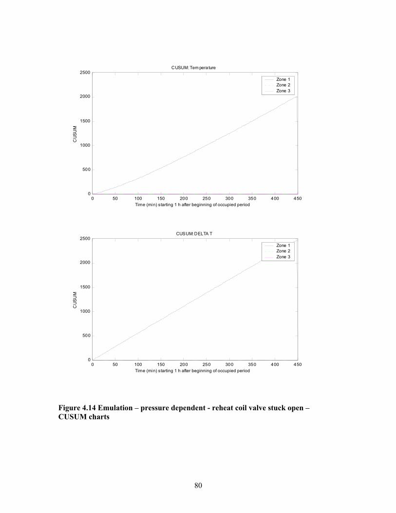
0 50 100 150 200 250 300 350 400 4500

500

1000

1500

2000

2500CUSUM: Tem perature

CUS

UM

Time (min) starting 1 h after beginning of occupied period

Zone 1Zone 2Zone 3

0 50 100 150 200 250 300 350 400 4500

500

1000

1500

2000

2500CUSUM: DELTA T

CUS

UM

Time (min) starting 1 h after beginning of occupied period

Zone 1Zone 2Zone 3

Figure 4.14 Emulation – pressure dependent - reheat coil valve stuck open – CUSUM charts

80

Tables 4.8 and 4.9 show a range of values for alarm limits for each CUSUM indicated. If the actual fault threshold (alarm limit) is less than the minimum shown, false alarms will be generated. If the threshold is greater than the maximum shown, some of the faults will not be detected. Therefore, using the values in Table 4.8 for the pressure independent VAV boxes will allow the detection of all the faults in the data set without any false alarms. Using the values in Table 4.9 for the pressure dependent VAV boxes will detect all of the detectable faults in the data set without any false alarms. As explained in the following paragraph, some faults will not be detected for pressure dependent VAV boxes. “Not used” in Tables 4.8 and 4.9 indicates that the limit was not needed to detect any of the faults that were implemented. These preliminary results do not constitute a rigorous statistical approach. Before definitive alarm limits can be established, additional data need to be collected across a range of VAV box types, cooling/heating/swing seasons, size ranges, and controller manufacturers. It may be necessary to adjust the alarm limits based on one or more of these parameters. For example, there might be a set of alarm limits for small VAV boxes, another for medium boxes, and another for large boxes.

Table 4.8: Pressure Independent VAV Box Alarm Limits

Minimum Alarm Limit Maximum Alarm Limit Airflow positive (S) 30 3300Airflow negative (T) 50 3200Temperature positive (S) 0 10 000Temperature negative (T) 1 3500DELTA T positive (S) 20 2800DELTA T negative (T) 0 Not used

Table 4.9: Pressure Dependent VAV Box Alarm Limits

Minimum Alarm Limit Maximum Alarm Limit Temperature positive (S) 9 2000Temperature negative (T) 60 1200DELTA T positive (S) 25 2400DELTA T negative (T) 8 Not used Tables 4.10 and 4.11 show the peak values of each CUSUM chart for the pressure independent and pressure dependent VAV boxes respectively. The bold values show where each CUSUM identified exceeds the alarm limits from Tables 4.8 and 4.9,

nt VAV .

Table 4.11 shows that the damper stuck open (heating and cooling seasons) and damper stuck closed (swing season) faults are not detected in the pressure dependent VAV boxes, but the reheat coil valve stuck open (swing and cooling seasons) and reheat coil valve

detecting a fault. Table 4.10 shows that all of the faults in the pressure independeboxes are detected

81

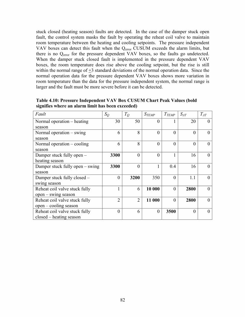
stuck closed (heating season) faults are detected. In the case of the damper stuck open ult, the control system masks the fault by operating the reheat coil valve to maintain fa

room temperature between the heating and cooling setpoints. The pressure independent VAV boxes can detect this fault when the Qerror CUSUM exceeds the alarm limits, but there is no Qerror for the pressure dependent VAV boxes, so the faults go undetected. When the damper stuck closed fault is implemented in the pressure dependent VAV boxes, the room temperature does rise above the cooling setpoint, but the rise is still within the normal range of +3 standard deviations of the normal operation data. Since the normal operation data for the pressure dependent VAV boxes shows more variation in room temperature than the data for the pressure independent system, the normal range is arger and the fault must be more severe before it can be detected. l

Table 4.10: Pressure Independent VAV Box CUSUM Chart Peak Values (bold signifies where an alarm limit has been exceeded)

Fault SQ TQ STEMP TTEMP S∆T T∆T Normal operation – heating season

30 50 0 1 20 0

Normal operation – swing 6 8 0 0 0 0season Normal operation – cooling

ason 6 8 0 0 0 0

seDamper stuck fully open – 3300 0 0 1 16 heating season

0

Damper stuck fully open – swing 3300 0 1 0.4 16 season

0

Damper stuck fully closed – 0 3200 350 0 1.1 swing season

0

Reheat coil valve stuck fully 1 6 10 000 0 2800 0open – swing season Reheat coil valve stuck fully open – cooling season

2 2 11 0 000 0 2800

Reheat coil valve stuck fully n

0 6 0 3500 0 closed – heating seaso

0

82

Table 4.11: Pressure Dependent VAV Box CUSUM Chart Peak Values (bold signifies where an alarm limit has been exceeded)

ault STEMP TTEMP S∆T T∆T ormal operation – heating

eason 0 60 25 8

ormal operation – swing eason

9 0 0 0

ormal operation – cooling eason

0 0 0 0

FNsNsNsDamper stuck fully open – h

0 14 17 0eating season amper stuck fully open – swing 0D

season 4 17 0

Damper stuck fully closed – swing season

0 0 12 0

Reheat coil valve stuck fully open 2000 0 2500 0– swing season Reheat coil valve stuck fully open 2300 0 2400 0– cooling season Reheat coil valve stuck fully 0 1200 25 0closed – heating season

5 SUMMARY AND FUTURE WORK a rule based DD or AH nd V CC, a istica

l based FDD tool for VAV boxes. APAR consists of a set of expert rules, rgy balances Control sig used de e th

ration, which identifies the subset of the rules to be evaluated. A by CSTB, a ows sim fie ssing HU data

et of process errors, valid for most VAV box control strategies, to nce. CUSUM charts, a statistic qu ontrol l, arrrors. Thresholds are determined by statistical analysis of a

database of “normal operation” data.

APAR was evaluated with laboratory, simulation, and emulation results. Using simulation data, APAR detected 10 of 20 faults during heating season, 14 of 20 faults during swing season, and 12 of 20 faults during cooling season. In addition, during swing season APAR was able to detect the presence of 2 VAV box faults. In the emulation, two systems (designated A and B) were used to generate data. Due to the real-time nature of the emulation, only a subset of the faults tested in simulation were studied. The emulation faults presented in this paper were those believed to have the largest impact on system operation. Using emulation data, APAR detected 3 out of 5 faults for Controller A, and 5 out of 5 for Controller B. Some of the missed faults could only be detected with additional sensors. For example, to detect a heating coil valve

This report describes APAR,quality contro

F tool f Us a PA stat l

derived from mass and eneAHU’s mode of ope

. nals are to termin e

graphical interface, developedVPACC uses a small s

ll pli d proce of A trend .

measure VAV box performaused to evaluate the process e

al ality c too e

83

leakage in winter would require the installation of an additional sensor, such as a APAR stem A

HU operation. In addition a false during normal operation was due to unstable control action taken by the system A

tem B data, APAR as able to t all fivefully detected every harmful fault implemented.

was evaluated using laboratory, simulation, and emulation results. The IEC epresents normal o ration as we as three fau . VPAC

d all three faults. Two of the four faults from simulation were detected. One of VAV box damper st k open, w not detect ecause th

dent controls masked the fault. The other fault, the VAV box reheat coil cted because the controls never attempted to open the

herefore, the fault had no impact on system operation. Two systems were : one was pressu independe the other s pressu

he pressure independent system detected all four of the faults considered, itions. ressure dep ndent im

o detect the VAV box damper stuck open fault because it was masked by ent impl ation of VP C also d the VA

closed fault because of the small impact this fault had. When provided pendent VAV box VPACC was able to detect every fault

false alarms. APAR and VPACC were evaluated using data from several different sources – laboratory

d emulation. Consistent results across these

l buildings.

temperature sensor between heating coil and cooling coil. Using system A data,was able to detect four of the five faults. The control strategy implemented by sycaused the undetected fault to have no impact on AalarmAHU controller. Using syssuccess

w detec faults. APAR

VPACClaboratory VAV box data rdetecte

pe ll lts C

the undetected faults, the pressure depen

uc as ed b e

valve stuck closed, was not detevalve; tevaluated in the emulationdependent. T

re nt, wa re

under a variety of weather condVPACC failed t

The p e plementation of

the controls. The pressure dependbox damper stuck

ement AC misse V

with data from pressure indeconsidered without any

es,

based AHUs and VAV boxes, simulation, andiverse testing environments, in combination with the laboratory testing to validate the fault models, gives a high level of confidence that not only will the FDD tools perform well in real buildings, but also that the test conditions reflect the conditions in real buildings. In the next phase of the project, additional trend data from other buildings will be collected in order to refine both FDD tools and to determine robust thresholds for VPACC. Ultimately, the tools will be embedded in local AHU and VAV box controllers and evaluated in the VCBT and in rea

84

6 REFERENCES [1] Fasolo, P.S., and Seborg, D.E., 1992, “ Fault Detection in HVAC Control Systems Using Statistical Quality Control Charts”, prepared for the California Institute for Energy Efficiency. [2] Bushby, S.T., Castro, N.S., Galler, M.A., Park, C., House, J.M., 2001, “Using the Virtual Cybernetic Building Testbed and FDD Test Shell for FDD Tool Development”,

ISTIR 6818.

E. Flynn. 1981. Abbreviation of Climate Data for uilding Thermal Analysis Programs Using Representative Samples of Various Lengths.

N [3] Centre Scientifique et Technique du Bâtiment, 2000, FDD_AHU1.1 [4] Park, C., Clark, D. R., and Kelly, G. E., An Overview of HVACSIM+, A Dynamic wBuilding/HVAC/Control Systems Simulation Program, Proceedings of the 1st Annual Building Energy Simulation Conference, Seattle, WA, August 21-22 (1985). [5] House, J.M., Vaezi-Nejad, H., and Whitcomb, J.M., 2001, “An Expert Rule Set for Fault Detection in Air-Handling Units,” ASHRAE Transactions, Vol. 107, Pt. 1: pp. 858-871. [6] Ryan, Thomas P., 2000, Statistical Methods for Quality Improvement, 2nd Edition, Wiley and Sons, New York. [7] Nall, D. H., E. A. Arens, and L. BASHRAE Transactions Vol. 87, Pt. 1: 923-934.

85

ATTACHMENT A: NOMENCLATURE FOR TABLE 1

ma = mixed air temperature

= changeover air temperature for switching between Modes 3 and 4 T = supply air temperature set point

Tsf = temperature rise across the supply fan

Q /Q = outdoor air fraction = (T - T )/(T - T )

= normalized heating coil valve control signal [0,1] with uhc = 0 indicating the valve is closed and uhc = 1 indicating it is 100 %

e control signal [0,1] with ucc = 0 indicating the valve is closed and u = 1 indicating it is 100 %

dindicating the outdoor air damper is closed and ud = 1 indicating it is 100 % open

εt = threshold parameter accounting for errors in temperature measurements

εf = threshold parameter accounting for errors related to airflows (function of uncertainties in temperature measurements)

εhc = threshold parameter for the heating coil valve control signal εcc = threshold parameter for the cooling coil valve control signal εd = threshold parameter associated with the mixing box damper control

signal MTmax = maximum allowable number of mode transitions per hour

Tsa = supply air temperature

T Tra = return air temperature Toa = outdoor air temperature Tco sa,s ∆ ∆Trf = temperature rise across the return fan ∆Tmin = threshold on the minimum temperature difference between the

return and outdoor air oa sa ma ra oa ra (Qoa/Qsa)min = threshold on the minimum outdoor air fraction uhc

open ucc = normalized cooling coil valv

ccopen

ud = normalized mixing box damper control signal [0,1] with u = 0

86