results of ambient rf environment and noise floor ... · pdf fileresults of ambient rf...

WORLD METEOROLOGICAL ORGANIZATION

_____________

COMMISSION FOR BASIC SYSTEMS STEERING GROUP ON RADIO FREQUENCY

COORDINATION

GENEVA 16-18 MARCH 2006

CBS/SG-RFC 2005/Doc. 5(1) _______

ITEM 5

ENGLISH only

Results of Ambient RF Environment and Noise Floor Measurements Taken in the U.S. in 2004 and 2005

(Submitted By Robert Leck, USA)

Summary and Purpose of Document This report details the results of a series of Radio Frequency (RF) Ambient Environment measurements. The measurements took place over a five-month period at the following National Oceanic and Atmospheric Administration (NOAA) facilities across the United States: NOAA NWS Weather Forecasting Offices, NOAA NWS Remote Weather Radar sites, and NOAA NESDIS Earth Station sites. RF Sampling took place in urban, suburban, airport, and rural areas and the RF ambient environment at these locations was measured, analyzed and tabulated. A summary of the results is presented here for use as a baseline for making future comparative measurements.

Action Proposed This document is provided for information to the SG-RFC. The SG-RFC may wish to discuss the need for similar tests in other regions of the world.

08/03/2006

Results of Ambient RF Environment and Noise Floor Measurements Taken in The U.S. in 2004 and 2005

1. Executive Overview NOAA operates a wide variety of very sensitive ground based and space borne meteorological observing and remote sensing systems. The potential deployment of new systems and services within the frequency bands that are currently used by NOAA has generated the need to measure and collect baseline noise floor data. The data will be used to quantify future deviations in current noise floor levels. (The “noise floor” in this context refers to the power spectral density of thermal noise plus the ambient signal background noise within a particular frequency band) This report details the results of a series of Radio Frequency (RF) Ambient Environment measurements. The measurements took place over a five-month period at the following NOAA facilities across the United States: NOAA NWS Weather Forecasting Offices, NOAA NWS Remote Weather Radar sites, and NOAA NESDIS Earth Station sites. RF sampling took place in urban, suburban, airport, and rural areas. The RF ambient environment at these locations was measured, analyzed and tabulated. A summary of the results is presented here for use as a baseline for making future comparative measurements. 2. Ambient RF Environment Measurement System (ARFEMS) Program

Objectives Principal areas of emphasis in this study include the measurement and profiling of the ambient noise floor in urban, suburban, rural, and airport environments. The data will be used as a reference baseline for impact testing during the deployment of new potentially interfering radio technologies and to address future regulatory changes. The baseline data, when combined with future tests, can help spectrum regulators make informed decisions when implementing new regulations and deploying new radio technologies. Specific objectives include:

• Profile the ambient noise floor within frequency bands, used by NOAA systems. • Identify existing services within the NOAA frequency bands of interest. • Establish an archived database. • Establish a basis for comparative measurements prior to, during, and after the

deployment of new radio technologies and U.S. and international regulatory changes. • Collect data as a basis of additional controlled interference studies.

The data collected in this analysis will provide a baseline, for future comparative studies, a reference for additional interference measurements, and can help regulators make informed decisions on any impact an increased noise floors may have on other system during deployment initiatives within the baselined frequency ranges. 3. ARFEMS Measurement Plan Overview The ambient environment measurements conducted in this analysis included RF ambient environment profiling across meteorological and space sciences frequency bands shown in Table 1 below.

08/03/2006

TABLE 1 – Frequency Bands of Interest

NWS NESDIS 162 - 174 MHz 136 – 138 MHz 23.6 – 24.1 GHz

400.15 – 420 MHz 400.15 – 403 MHz 25.5 – 27 GHz 440 – 460 MHz 406 – 406.1 MHz 31.3 – 31.5 GHz

1670 – 1700 MHz 1541 –1545 MHz 35.9 – 37.1 GHZ 2700 – 3000 MHz 2000 – 2300 MHz 50.2 – 60.6 GHz 5600 – 5650 MHz 6400 – 6800 MHz 9300 – 9500 MHz 7450 – 7830 MHz

8025 – 8375 MHz 10.6 18.8 GHz 3.1 Site Selection Site selection was based upon a number of factors such as: site access (location), environment (Urban, Suburban, Airport, etc.) function (Weather Radar, Satellite Earth Station, etc.) and facilities (equipment access, power, etc.). Since it was impossible to test every NOAA site, a typical set of sites in urban, suburban, and rural locations were selected from weather forecasting offices, remote radar sites, satellite earth stations and airport environments. The sites selected for the ambient measurement analysis are shown in Figure 3. Green diamonds indicate sites where measurements were taken and red diamonds indicate candidate sites where future measurements could be conducted.

Figure 3 – Measurement Site Locations

08/03/2006

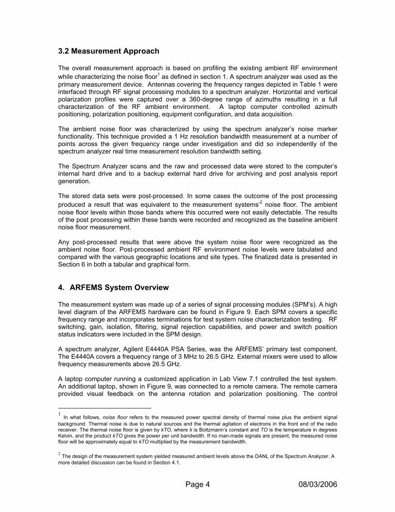
3.2 Measurement Approach The overall measurement approach is based on profiling the existing ambient RF environment while characterizing the noise floor1 as defined in section 1. A spectrum analyzer was used as the primary measurement device. Antennas covering the frequency ranges depicted in Table 1 were interfaced through RF signal processing modules to a spectrum analyzer. Horizontal and vertical polarization profiles were captured over a 360-degree range of azimuths resulting in a full characterization of the RF ambient environment. A laptop computer controlled azimuth positioning, polarization positioning, equipment configuration, and data acquisition. The ambient noise floor was characterized by using the spectrum analyzer’s noise marker functionality. This technique provided a 1 Hz resolution bandwidth measurement at a number of points across the given frequency range under investigation and did so independently of the spectrum analyzer real time measurement resolution bandwidth setting. The Spectrum Analyzer scans and the raw and processed data were stored to the computer’s internal hard drive and to a backup external hard drive for archiving and post analysis report generation. The stored data sets were post-processed. In some cases the outcome of the post processing produced a result that was equivalent to the measurement systems’2 noise floor. The ambient noise floor levels within those bands where this occurred were not easily detectable. The results of the post processing within these bands were recorded and recognized as the baseline ambient noise floor measurement. Any post-processed results that were above the system noise floor were recognized as the ambient noise floor. Post-processed ambient RF environment noise levels were tabulated and compared with the various geographic locations and site types. The finalized data is presented in Section 6 in both a tabular and graphical form. 4. ARFEMS System Overview The measurement system was made up of a series of signal processing modules (SPM’s). A high level diagram of the ARFEMS hardware can be found in Figure 9. Each SPM covers a specific frequency range and incorporates terminations for test system noise characterization testing. RF switching, gain, isolation, filtering, signal rejection capabilities, and power and switch position status indicators were included in the SPM design. A spectrum analyzer, Agilent E4440A PSA Series, was the ARFEMS’ primary test component. The E4440A covers a frequency range of 3 MHz to 26.5 GHz. External mixers were used to allow frequency measurements above 26.5 GHz. A laptop computer running a customized application in Lab View 7.1 controlled the test system. An additional laptop, shown in Figure 9, was connected to a remote camera. The remote camera provided visual feedback on the antenna rotation and polarization positioning. The control

1 In what follows, noise floor refers to the measured power spectral density of thermal noise plus the ambient signal background. Thermal noise is due to natural sources and the thermal agitation of electrons in the front end of the radio receiver. The thermal noise floor is given by kTO, where k is Boltzmann’s constant and TO is the temperature in degrees Kelvin, and the product kTO gives the power per unit bandwidth. If no man-made signals are present, the measured noise floor will be approximately equal to kTO multiplied by the measurement bandwidth. 2 The design of the measurement system yielded measured ambient levels above the DANL of the Spectrum Analyzer. A more detailed discussion can be found in Section 4.1.

08/03/2006

computers were typically located at least 50 meters from the measurement system. To provide a display of real-time measurement activity, an LCD monitor was connected to the spectrum analyzer through a VGA extender.

Figure 9 – System Diagram

Horn Antennas

Ethernet

RemoteVideo Camera

Laptop For Remote Video Camera

VariableAzimuth Drive RS-232

Hub

Ethernet

Ethernet

GPIB/Ethern teConverter

Remote Spectrum Analyzer Monitor

Spectrum Analyzer

Laptop w/Lab View

Frequency Range N

Frequency Range Y

Frequency Range X

Frequency Range N

Frequency Range 2

Frequency Range 1

RF

Ethernet

Above 26 GHz

Direct To Spectrum Analyzer

Direct To Spectrum Analyzer Harmonic

Mixer

Harmonic Mixer

Temperature Sensor

CoaxialSwitch

Bandpass Filter LNA

Bandpass Filter LNA

Bandpass Filter LNA

Bandpass LNA

Photographs of the assembled system can be found in Figure 10.

Figure 10 – Assembled ARFEMS System

08/03/2006

A more detailed photograph of a typical signal processing module and the computer/control systems can be seen in Figure 11.

Figure 11 – SPM and Computer/Control Systems

NOAA will maintain the measurement systems hardware and software for use in future interference and protection criteria studies. 4.1 Individual Component and System Testing The Measurement System (SPM’s, Control Circuitry, Power Supplies, Azimuth and Polarization Drives and Operational Testing and Field Measurement Software) was designed, built, and integrated by NOAA using high quality hardware and test equipment. Simulations were run to verify the SPM designs and every active (LNA’s, RF Switches, Drive Motors, Control Relays, LED’s, etc.) and passive (Terminations, Feedthrough’s, etc.) component was tested before being incorporated into system assemblies. When all of the individual sub-systems were completed they were integrated into the final system. The assembled system was tested to verify its operation. Operational verification was performed on a system level. A summary of the required SPM MDS level, the measured SPM MDS level, the SPM noise Figure, noise floor, gain and system sensitivity test results can be found in Table 3.

08/03/2006

Table 3 – Requires MDS/System Level Test Results Summary

MDS SPM Performance Summary

Frequency Range (MHz - GHz)

Required (dBm)*

Measured (dBm)**

Margin Noise Figure

Noise Floor (dBm)**

Gain (dBm)

System Sensitivity

136 MHz - 174 MHz -114 -175 62 5.1 -152 26 -178 400 MHz - 460 MHz -137 -176 39 5.1 -153 26 -179 1.54 GHz - 2.00 GHz -147 -169 22 5.9 -151 27 -178

2.00 GHz - 3 GHz -146 -165 19 6.9 -141 27 -168 5.6 GHz - 7.830 GHz -164 -167 3 2.9 -132 38 -171 8.025GHz - 9.5 GHz -119 -168 49 3.0 -135 35 -170 10.6 GHz - 12 GHz -133 -166 33 4.7 -132 35 -167 12 GHZ - 18 GHz -125 -163 38 2.8 -136 30 -169

18 GHz - 26.5 GHz -139 -160 21 3.9 -138 27 -165 26.5 GHz - 40 GHz -136 -156 20 Not Measured -97 60 -158

* Most Stringent Criteria ** Measurement Uncertainty +-3 dB The Signal Processing Modules (SPM’s) noise floor levels limited the overall systems noise floor performance. This fact did not have a negative impact on collection of baseline data as the measured MDS (Minimum Detectable Signal) levels of the SPM’s were, as shown in Figure 12, well below the required SPM MDS levels. (The required SPM MDS levels were derived using the minimum interference levels of the targeted NOAA systems as the basis of the calculation.3) When compared with the required MDS levels, the measured MDS levels yielded positive margins throughout the entire range of measurements

Figure 12 – Required vs. Measured SPM MDS

136

MH

z - 1

74 M

Hz

400

MH

z - 4

60 M

Hz

1.54

GH

z - 2

.00

GH

z

2.00

GH

z - 3

GH

z

5.6

GH

z - 7

.830

GH

z

8.02

5GH

z - 9

.5 G

Hz

10.6

GH

z - 1

2 G

Hz

12 G

HZ

- 18

GH

z

18 G

Hz

- 26

.5 G

Hz

26.5

GH

z - 4

0 G

Hz

-180

-170

-160

-150

-140

-130

-120

Measured MDS Required MDS

3 Detailed Interference Thresholds and MDS calculations can be found in the various ITU Recommendations, which have been listed as references. Additional interference threshold calculations were based upon a previous analysis. (RFI Analysis for Registered Users near FCDAS).

08/03/2006

In terms of overall noise performance, the system was designed to provide sufficient gain as to overcome the noise limitations posed by the DANL of the Spectrum Analyzer. The system could not, however, overcome the noise measurement limitations posed by the presence of fundamental thermal noise in the measurement system. 4.2 Operational Software Overview The AREFMS control software was developed using a Windows based Lab View 7.1 programming environment. The program controls the flow of the data acquisition process. It also controls azimuth and polarization positioning, spectrum analyzer, temperature measurements and data storage.

The software leads users through a series of tasks and measurement sequences for each of the frequency ranges of interest. The three basic processes are: 1) Noise Characterization, 2) Ambient RF Environment Measurements and 3) Data Collection and Storage.

The first step of the process was to characterize the SPM noise performance. Once Noise Characterization was completed, a comparison was made to the original (lab) SPM noise characterization to verify proper operation of the SPM. A change in the noise characterization could indicate a system failure resulting in decreased sensitivity or increased internal noise. The next step was to measure the ambient RF environment. The azimuth and polarization were varied sequentially and the Spectrum analyzer was instructed to take a scan across the frequency band of interest. In the final step the resultant scan was stored to the Laptop Computer hard drive. At the close of each session a back up of the collected data was written to an external hard drive and written to a CD.

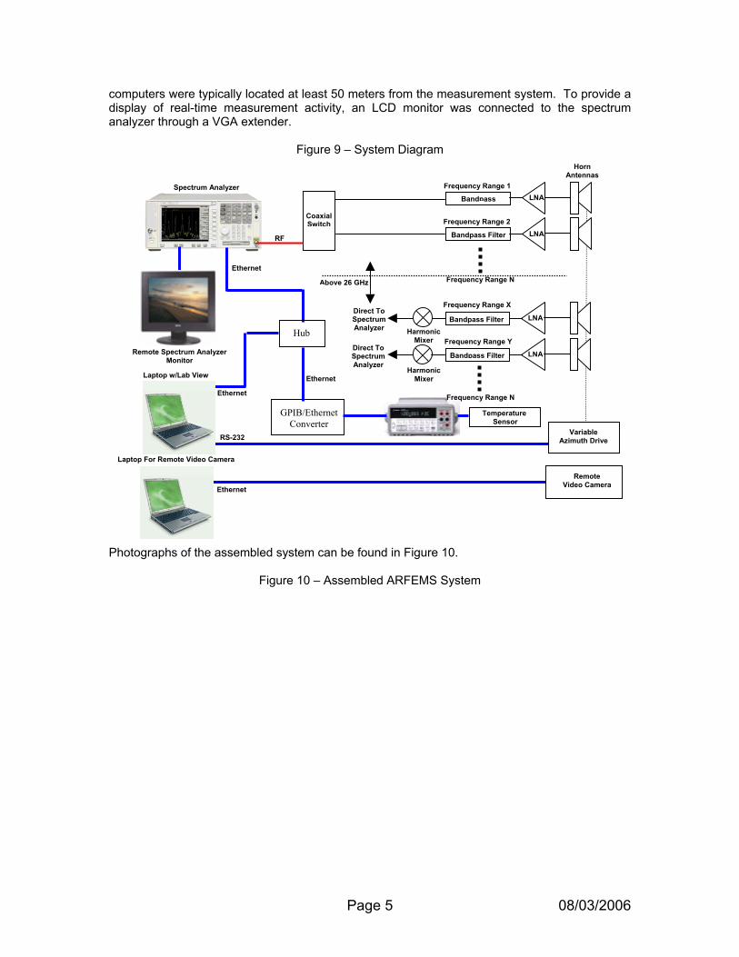
The ARFEMS primary user interface screen is shown in Figure 13. Additional screens (Normal Run Mode, System Test Mode, SPM Noise Characterization, Interference Measurements, Ambient Environment Measurements, etc.) are all accessed through this interface.

Figure 13 – ARFEMS User Interface Main Screen

08/03/2006

08/03/2006

4.3 Measurement Procedure Overview

The objective of this testing was to characterize the Ambient RF Environment and noise floor of each frequency range of interest.4 (See Section 3) Measurements were made to characterize the ambient RF environment and noise floor. As mentioned in Section 4.2, there were three basic operational processes: 1) Noise Characterization, 2) Ambient RF Environment Measurements and 3) Data Collection and Storage. The first step in the process was to characterize the noise contributions of the Spectrum Analyzer and the SPM. Figure 14 illustrates the test setup used for the noise characterization and ambient noise measurements.

Figure 14 – Noise Characterization Test Setup Block Diagram

Printer

Parallel

To facilitatSPM’s. Th

ANTEN

TempSe

To acquiresignal pathof interest

4 The intent obackground nbelow the ex

Azimuth and Polarization Drive Motors

APC

Antenna/Signal Processing Module/ ASPM

Spectrum Analyzer

Power Supply

Relay Block

Toshiba Laptop

Computer

USB

GPIB To Ethernet Adaptor

Multimeter

RS232

GPIB

External Hard Drive

HUB Extended VGA

Ethernet

ExternalSpectrum Analyzer

LCD Monitor

e this process, 50-ohm terminations were added to the signal paths within the various e positions of these 50-ohm terminations are shown in Figure 15.

Figure 15 – Generic SPM Block Diagram

NA

RF SWITCH 3

LNA

RF SWITCH 1

SPECTRUM ANALYZER

Agilent E4440A DC – 26.5 GHZ

50-Ohm Termination

Temperature Sensor

ISOLATOR BANDPASS FILTER

50-Ohm Termination

erature nsor

the noise characterization data, the terminations were switched in and out of the in sequence and the noise power levels were measured across the frequency range

. Switching RF Switch 3 to the terminated position gives the SA DANL (Spectrum

f the measurement program was not to detect the ambient thermal background noise, the ambient thermal oise is so low it may not be detectable above the system noise floor, but too measure to an ambient level

isting NOAA and NESDIS System interference thresholds.

08/03/2006

Analyzer Displayed Average Noise Floor). Switching RF Switch 1 to the terminated position provides a measurement of the SPM (Signal Processing Module) noise floor. This data was stored for use during the post processing process and a comparison was made to previously measured Lab Noise Characterization data, which was captured during the system testing process. The system was deemed to be operating properly if there was no difference between the field and the lab noise characterization data. A graphical representation of the Noise Characterization Data as it appeared on the screen of the spectrum analyzer, the actual trace and noise marker data points and the spectrum analyzer’s trace and state data were linked to a primary data acquisition spreadsheet and were stored on digital media in Excel, CSV (Coma Separated Variable), Image and Trace+State formats. The next step was to measure the ambient RF Environment and acquire trace and noise marker data over the frequency range of interest. This process was one in which a test antenna was connected to the Signal Processing Module. The Antenna and Signal Processing Module were, in most cases, affixed to an antenna mast. This mast was mounted to the Azimuth Drive. System power supplies, the Spectrum Analyzer, Voltmeters, control electronics and interface extenders were secured within a portable rack enclosure. (In the event of inclement weather the entire “system” was placed under a canopy for protection.) The antenna was rotated through a 360-degree arc in pre-defined steps. (The step size was a function of the test antenna beam width and varied from SPM to SPM.) The antenna polarization was set to an initial starting position (horizontal or vertical) and the Spectrum Analyzer was instructed to take a sweep. The Spectrum analyzer was set to a specific center frequency and span, resolution bandwidth and video bandwidth. The number of data points and number of noise marker points were selected programmatically. (See Table 4 – Measurement and Data Collection Settings.)

Table 4 – Measurement and Data Collection Settings

ARFEMS SPM Frequency Range Measurement Range Span (MHz)

# Data Points RBW/VBW

Noise MarkerPoints

136 MHz - 174 MHz 136 MHz to 138 MHz 2 601 100 Hz 120

162 MHz to 174 MHz 12 601 1 kHz 120

400 MHz - 460 MHz 400 MHz - 420 MHz 20 601 3 kHz 120

440 MHz - 460 MHz 20 601 3 kHz 120

1.54 GHz - 2.00 GHz 1.54 GHz - 1.545 GHz 5 601 1 kHz 120

1.670 GHz - 1700 GHz 30 990 5.1 kHz 99

2.00 GHz - 3 GHz 2 GHz - 2.3 GHz 300 900 10 kHz 90

2.7 GHz - 3.0 GHz 300 900 10 kHz 90

5.6 GHz - 7.830 GHz 5.6 GHz - 5.650 GHz 50 150 3 kHz 15

6.4 GHz - 6.8 GHz 400 1200 10 kHz 120

7.450 GHz - 7.830 GHz 380 1140 10kHz 114

8.025GHz - 9.5 GHz 8.025 GHz - 8.375 GHz 350 1050 10 kHz 105

9.3 GHz - 9.5 GHz 200 600 10 kHz 60

10.6 GHz - 12 GHz 10.6 GHz - 11.3 GHz 700 2100 10 kHz 210

12 GHZ - 18 GHz 17.6GHz - 18 GHz 400 1200 10 kHz 120

18 GHz - 26.5 GHz 18 GHz - 18.5 GHz 500 1500 10 kHz 150

18.5 GHz - 19 GHz 500 1500 10 kHz 150

23.6 GHz - 24.1 GHz 500 1500 10 kHz 150

25.5 GHz - 26.25 GHz 750 2250 10 kHz 225

26.25 GHz - 27 GHz 750 2250 10 kHz 225

26.5 GHz - 40 GHz 26.5 GHz - 28 GHz 1500 4500 30 kHz 225

31.3 GHz - 31.5 GHz 200 600 30 kHz 60

35.9 GHz - 37.1 GHz 1200 3600 30 kHz 180

08/03/2006

A graphical representation of the Trace Data as it appeared on the screen of the spectrum analyzer, the actual trace and noise marker data points and the spectrum analyzer’s trace and state data were linked to a primary data acquisition spreadsheet and stored on digital media in Excel, CSV, Image and Trace+State formats. The antenna’s polarization was then switched and another set of measurements were taken, linked and stored. The azimuth was changed and the process continued until a full 360 degrees of measurement in azimuth for both horizontal and vertical polarizations was completed. If the SPM covered multiple sub-bands, all sub-bands were measured before antenna movement in order to reduce the antenna positioning time. The measured data was post-processed by operating on the captured Trace and Noise Marker data files. The measured data was compensated in order to provide received signal levels within a 1 Hz Resolution Bandwidth. A more detailed explanation of the data reduction, compensation and post processing process can be found in Section 5, ARFEMS Data Analysis Methodology. This data was used to determine the ambient noise floor and is tabulated and segmented in Section 6, ARFEMS Measurement Results. 5. ARFEMS Data Processing Methodology 5.1 Overview

The data processing process is made up of two steps: data reduction, and data analysis.

1. The Data Reduction section outlines the data reduction process. 2. The Data Analysis section is made up of two segments; 1) ambient noise floor and

ambient RF environment data processing and 2) data categorization (In this step the noise floor data is categorized as a function of measurement range, azimuth, polarization, site and environment (Urban, Suburban, Rural, Airport, environments).

5.2 Data Reduction The data reduction methodology is one through which the acquired measurement data is processed. The result of this processing yields the actual RF Ambient Signal and Ambient Noise Level as seen at the receiving antenna. The resultant data will be used as a baseline against which future field measurements will be compared. The purpose, as outlined earlier, in making these comparisons will be to determine if any changes to the ambient noise floor have taken place as the result of the deployment of new communications technology or change in regulations. In order to be able to accomplish this task, the trace and noise marker data was processed to compensate for system gains and losses and, where appropriate, converted to reflect a measurement resolution bandwidth of 1 Hz.5 An Excel Macro was written to operate on all the collected measurement data sets. Although some of the calculations were performed in mW (for addition and subtraction purposes), the final

5 Our original intent was to characterize the noise contribution of the SPM and compensate for it in the data correction computations. This would have added an additional level of compensation. Unfortunately, this could not be implemented as the ambient noise levels were, in most cases, buried in the measurement system noise and could not be mathematically extracted for data reduction or data compensation purposes.

08/03/2006

results were converted to and expressed in dBm. A simplified version of the data processing block diagram will be used for discussion purposes and is illustrated in Figure 17.

08/03/2006

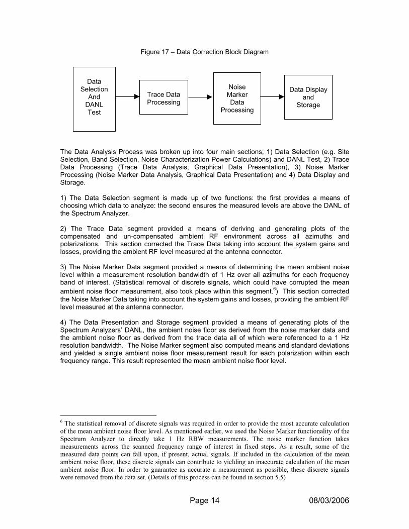
Figure 17 – Data Correction Block Diagram

Noise

Marker Data

Processing

Data Display

and Storage

Trace DataProcessing

Data

Selection And

DANL Test

The Data Analysis Process was broken up into four main sections; 1) Data Selection (e.g. Site Selection, Band Selection, Noise Characterization Power Calculations) and DANL Test, 2) Trace Data Processing (Trace Data Analysis, Graphical Data Presentation), 3) Noise Marker Processing (Noise Marker Data Analysis, Graphical Data Presentation) and 4) Data Display and Storage. 1) The Data Selection segment is made up of two functions: the first provides a means of choosing which data to analyze: the second ensures the measured levels are above the DANL of the Spectrum Analyzer. 2) The Trace Data segment provided a means of deriving and generating plots of the compensated and un-compensated ambient RF environment across all azimuths and polarizations. This section corrected the Trace Data taking into account the system gains and losses, providing the ambient RF level measured at the antenna connector. 3) The Noise Marker Data segment provided a means of determining the mean ambient noise level within a measurement resolution bandwidth of 1 Hz over all azimuths for each frequency band of interest. (Statistical removal of discrete signals, which could have corrupted the mean ambient noise floor measurement, also took place within this segment.6) This section corrected the Noise Marker Data taking into account the system gains and losses, providing the ambient RF level measured at the antenna connector. 4) The Data Presentation and Storage segment provided a means of generating plots of the Spectrum Analyzers’ DANL, the ambient noise floor as derived from the noise marker data and the ambient noise floor as derived from the trace data all of which were referenced to a 1 Hz resolution bandwidth. The Noise Marker segment also computed means and standard deviations and yielded a single ambient noise floor measurement result for each polarization within each frequency range. This result represented the mean ambient noise floor level.

6 The statistical removal of discrete signals was required in order to provide the most accurate calculation of the mean ambient noise floor level. As mentioned earlier, we used the Noise Marker functionality of the Spectrum Analyzer to directly take 1 Hz RBW measurements. The noise marker function takes measurements across the scanned frequency range of interest in fixed steps. As a result, some of the measured data points can fall upon, if present, actual signals. If included in the calculation of the mean ambient noise floor, these discrete signals can contribute to yielding an inaccurate calculation of the mean ambient noise floor. In order to guarantee as accurate a measurement as possible, these discrete signals were removed from the data set. (Details of this process can be found in section 5.5)

08/03/2006

6. ARFEMS Measurement Results The measurement results are tabulated in Section 6.1. The ambient noise floor results were derived from the Noise Marker Data as outlined in Section 5, Data Correction and Analysis. In summary, the Ambient Noise Floor was measured for each scan using the Spectrum Analyzer Noise Marker Function. Care was taken to avoid signals, which could contribute to errors in the Ambient Noise Floor calculation by statistically removing them from the Noise Marker data. The results of the Data Analysis process were combined and averaged as a function of frequency range and environment (Urban, Suburban, Rural, Airport). Means and standard deviations were computed for each of the measurement data arrays. Tabular summaries of this data can be found in Tables 10 and 11. Future comparative studies can use this data for quantifying changes in the ambient noise floor by comparing new measurements to the previously acquired data.

08/03/2006

6.1 Horizontally Polarized Data Table 10 summarizes the data as a function of Measurement Range and Environment for Horizontally polarized measurements.

Table 10 – Mean Ambient Noise Floor Levels As A Function of Environment and Frequency (Horizontal Polarization)

Measurement Range Urban Suburban Rural Airport

136 MHz - 138 MHz -142.2 -144.5 -144.8 -148.4

162 MHz - 174 MHz -142 -147.1 -147 -147.1

400 MHz - 420 MHz -163.7 -165.1 -165.7 -167.7

440 MHz - 460 MHz -164.9 -166.3 -166.9 -168.2

1.54 GHz - 1.545 GHz -166.9 -167.4 -168.4 -167.6

1.670 GHz - 1700 GHz -166.9 -167.1 -167.9 -167.2

2 GHz - 2.3 GHz -167.1 -166.8 -167.1 -166.6

2.7 GHz - 3.0 GHz -167.8 -167.5 -168 -167.5

5.6 GHz - 5.650 GHz -172.8 -173 -172.8 -172.9

6.4 GHz - 6.8 GHz -174.2 -174.2 -174.2 -174.2

7.450 GHz - 7.830 GHz -174.7 -174.9 -175.1 -174.9

8.025 GHz - 8.375 GHz -172.3 -173.1 -173.9 -173.2

9.3 GHz - 9.5 GHz -173.9 -174.9 -175.9 -175.1

10.6 GHz - 11.3 GHz -170.7 -171.4 -171.8 -170.6

17.6GHz - 18 GHz -173.2 -175.8 -174.9 -176.0

18 GHz - 18.5 GHz -170.4 -171.5 -172.4 -172.0

18.5 GHz - 19 GHz -171.7 -172.6 -173.6 -172.8

23.6 GHz - 24.1 GHz -165.8 -167.9 -167.6 -168

25.5 GHz – 26.25 GHz -164.0 -166.4 -167.1 -165.0

26.25 GHz - 27 GHz -165.1 -169.5 -168.4 -167.2

31.3 GHz - 31.5 GHz X X X X

35.9 GHz - 37.1 GHz X X X X

08/03/2006

Figures 34 through 37 illustrate this data on a per site basis.

136

MH

z-13

8 M

Hz

162

MH

z-17

4 M

Hz

400

MH

z-42

0 M

Hz

440

MH

z-46

0 M

HZ

1.54

GH

z-1.

545

MH

z

1.67

0 G

Hz-

1.70

0 G

Hz

2 G

Hz-

2.3

GH

z

2.7

GH

z-3.

0 G

Hz

5.6

GH

z-5.

650

GH

z

6.4

GH

z-6.

8 G

HZ

7.45

GH

z-7.

83 G

Hz

8.02

5 G

Hz-

8.37

5 G

Hz

9.3

GH

z-9.

5 G

Hz

10.6

GH

z-11

.3 G

Hz

17.6

GH

z- 1

8 G

Hz

18 G

Hz-

18.5

GH

z

18.5

GH

z-19

GH

z

23.6

GH

z-24

.1 G

Hz

25.5

GH

z-26

.25

GH

z

26.2

5 G

Hz

- 27.

0 G

Hz

31.3

GH

z-31

.5 G

Hz

35.9

GH

z-37

.1 G

Hz

-200

-180

-160

-140

-120

-100

Am

bien

t Noi

se L

evel

(dB

m)

Measured Frequency Ranges

Figure 34 - Urban Environment Ambient Noise Level(Horizontal Polarization)

136

MH

z-13

8 M

Hz

162

MH

z-17

4 M

Hz

400

MH

z-42

0 M

Hz

440

MH

z-46

0 M

HZ

1.54

GH

z-1.

545

MH

z

1.67

0 G

Hz-

1.70

0 G

Hz

2 G

Hz-

2.3

GH

z

2.7

GH

z-3.

0 G

Hz

5.6

GH

z-5.

650

GH

z

6.4

GH

z-6.

8 G

HZ

7.45

GH

z-7.

83 G

Hz

8.02

5 G

Hz-

8.37

5 G

Hz

9.3

GH

z-9.

5 G

Hz

10.6

GH

z-11

.3 G

Hz

17.6

GH

z- 1

8 G

Hz

18 G

Hz-

18.5

GH

z

18.5

GH

z-19

GH

z

23.6

GH

z-24

.1 G

Hz

25.5

GH

z-26

.25

GH

z

26.2

5 G

Hz

- 27.

0 G

Hz

31.3

GH

z-31

.5 G

Hz

35.9

GH

z-37

.1 G

Hz

-200

-180

-160

-140

-120

-100

Am

bien

t Noi

se L

evel

(dB

m)


Figure 35 - Suburban Environment Ambient Noise Level(Horizontal Polarization)

08/03/2006

136

MH

z-13

8 M

Hz

162

MH

z-17

4 M

Hz

400

MH

z-42

0 M

Hz

440

MH

z-46

0 M

HZ

1.54

GH

z-1.

545

MH

z

1.67

0 G

Hz-

1.70

0 G

Hz

2 G

Hz-

2.3

GH

z

2.7

GH

z-3.

0 G

Hz

5.6

GH

z-5.

650

GH

z

6.4

GH

z-6.

8 G

HZ

7.45

GH

z-7.

83 G

Hz

8.02

5 G

Hz-

8.37

5 G

Hz

9.3

GH

z-9.

5 G

Hz

10.6

GH

z-11

.3 G

Hz

17.6

GH

z- 1

8 G

Hz

18 G

Hz-

18.5

GH

z

18.5

GH

z-19

GH

z

23.6

GH

z-24

.1 G

Hz

25.5

GH

z-26

.25

GH

z

26.2

5 G

Hz

- 27.

0 G

Hz

31.3

GH

z-31

.5 G

Hz

35.9

GH

z-37

.1 G

Hz

-200

-180

-160

-140

-120

-100

Am

bien

t Noi

se L

evel

(dB

m)


Figure 36 - Rural Environment Ambient Noise Level(Horizontal Polarization)

136

MH

z-13

8 M

Hz

162

MH

z-17

4 M

Hz

400

MH

z-42

0 M

Hz

440

MH

z-46

0 M

HZ

1.54

GH

z-1.

545

MH

z

1.67

0 G

Hz-

1.70

0 G

Hz

2 G

Hz-

2.3

GH

z

2.7

GH

z-3.

0 G

Hz

5.6

GH

z-5.

650

GH

z

6.4

GH

z-6.

8 G

HZ

7.45

GH

z-7.

83 G

Hz

8.02

5 G

Hz-

8.37

5 G

Hz

9.3

GH

z-9.

5 G

Hz

10.6

GH

z-11

.3 G

Hz

17.6

GH

z- 1

8 G

Hz

18 G

Hz-

18.5

GH

z

18.5

GH

z-19

GH

z

23.6

GH

z-24

.1 G

Hz

25.5

GH

z-26

.25

GH

z

26.2

5 G

Hz

- 27.

0 G

Hz

31.3

GH

z-31

.5 G

Hz

35.9

GH

z-37

.1 G

Hz

-200

-180

-160

-140

-120

-100

Am

bien

t Noi

se L

evel

(dB

m)


Figure 37 - Airport Environment Ambient Noise Level(Horizontal Polarization)

08/03/2006

Figure 38 compares the ambient noise levels of each of the sites from an environmental perspective. (The radial axis represents the measured frequency band. The circular axis represents the ambient noise level.)

Figure 38 - Ambient Noise Level(Horizontal Polarization)

-200

-190

-180

-170

-160

-150

-140

-130136 MHz-138 MHz

162 MHz-174 MHz

400 MHz-420 MHz

440 MHz-460 MHZ

1.54 GHz-1.545 MHz

1.670 GHz-1.700 GHz

2 GHz-2.3 GHz

2.7 GHz-3.0 GHz

5.6 GHz-5.650 GHz

6.4 GHz-6.8 GHZ

7.45 GHz-7.83 GHz

8.025 GHz-8.375 GHz

9.3 GHz-9.5 GHz

10.6 GHz-11.3 GHz

17.6GHz- 18 GHz

18 GHz-18.5 GHz

18.5 GHz-19 GHz

23.6 GHz-24.1 GHz

25.5 GHz-26.25 GHz

26.25 GHz - 27.0 GHz

Urban Suburban Rural Airport

08/03/2006

6.2 Vertically Polarized Data Table 11 summarizes the data as a function of Measurement Range and Environment for Vertically polarized measurements.

Table 11 – Mean Ambient Noise Floor Levels As A Function of Environment and Frequency (Vertical Polarization)

Measurement Range Urban Suburban Rural Airport

136 MHz - 138 MHz -141.5 -142.2 -141.7 -145

162 MHz - 174 MHz -141.9 -145.5 -141.4 -146.2

400 MHz - 420 MHz -164.4 -166.3 -167.2 -168.2

440 MHz - 460 MHz -164.6 -166.6 -167.6 -168.7

1.54 GHz - 1.545 GHz -167 -167.2 -168.4 -167.7

1.670 GHz - 1700 GHz -166.8 -167.1 -167.9 -167.3

2 GHz - 2.3 GHz -167.1 -166.8 -167.1 -166.6

2.7 GHz - 3.0 GHz -167.8 -167.5 -167.9 -167.4

5.6 GHz - 5.650 GHz -172.7 -172.8 -172.7 -173

6.4 GHz - 6.8 GHz -173.8 -174.1 -174.2 -174.4

7.450 GHz - 7.830 GHz -174.4 -174.8 -175.1 -175

8.025 GHz - 8.375 GHz -172.5 -172.9 -173.7 -173

9.3 GHz - 9.5 GHz -174.1 -174.8 -175.8 -175

10.6 GHz - 11.3 GHz -170.9 -171.5 -171.9 -170.7

17.6GHz - 18 GHz -173.1 -175.4 -175.1 -175.8

18 GHz - 18.5 GHz -170.8 -171.8 -175.25 -171.6

18.5 GHz - 19 GHz -171.7 -173 -173.45 -172.8

23.6 GHz - 24.1 GHz -170.3 -169.4 -167.72 -168

25.5 GHz – 26.25 GHz -166.1 -166. -167.04 -166.3

26.25 GHz - 27 GHz -167.1 -167.9 -168.25 -167.2

31.3 GHz - 31.5 GHz X X X X

35.9 GHz - 37.1 GHz X X X X

08/03/2006

Figures 39 through 43 illustrate this data on a per site basis.

136

MH

z-13

8 M

Hz

162

MH

z-17

4 M

Hz

400

MH

z-42

0 M

Hz

440

MH

z-46

0 M

HZ

1.54

GH

z-1.

545

MH

z

1.67

0 G

Hz-

1.70

0 G

Hz

2 G

Hz-

2.3

GH

z

2.7

GH

z-3.

0 G

Hz

5.6

GH

z-5.

650

GH

z

6.4

GH

z-6.

8 G

HZ

7.45

GH

z-7.

83 G

Hz

8.02

5 G

Hz-

8.37

5 G

Hz

9.3

GH

z-9.

5 G

Hz

10.6

GH

z-11

.3 G

Hz

17.6

GH

z- 1

8 G

Hz

18 G

Hz-

18.5

GH

z

18.5

GH

z-19

GH

z

23.6

GH

z-24

.1 G

Hz

25.5

GH

z-26

.25

GH

z

26.2

5 G

Hz

- 27.

0 G

Hz

31.3

GH

z-31

.5 G

Hz

35.9

GH

z-37

.1 G

Hz

-200

-180

-160

-140

-120

-100

Am

bien

t Noi

se L

evel

(dB

m)


Figure 39 - Urban Environment Ambient Noise Level(Vertical Polarization)

136

MH

z-13

8 M

Hz

162

MH

z-17

4 M

Hz

400

MH

z-42

0 M

Hz

440

MH

z-46

0 M

HZ

1.54

GH

z-1.

545

MH

z

1.67

0 G

Hz-

1.70

0 G

Hz

2 G

Hz-

2.3

GH

z

2.7

GH

z-3.

0 G

Hz

5.6

GH

z-5.

650

GH

z

6.4

GH

z-6.

8 G

HZ

7.45

GH

z-7.

83 G

Hz

8.02

5 G

Hz-

8.37

5 G

Hz

9.3

GH

z-9.

5 G

Hz

10.6

GH

z-11

.3 G

Hz

17.6

GH

z- 1

8 G

Hz

18 G

Hz-

18.5

GH

z

18.5

GH

z-19

GH

z

23.6

GH

z-24

.1 G

Hz

25.5

GH

z-26

.25

GH

z

26.2

5 G

Hz

- 27.

0 G

Hz

31.3

GH

z-31

.5 G

Hz

35.9

GH

z-37

.1 G

Hz

-200

-180

-160

-140

-120

-100

Am

bien

t Noi

se L

evel

(dB

m)


Figure 40 - Suburban Environment Ambient Noise Level(Vertical Polarization)

08/03/2006

13

6 M

Hz-

138

MH

z

162

MH

z-17

4 M

Hz

400

MH

z-42

0 M

Hz

440

MH

z-46

0 M

HZ

1.54

GH

z-1.

545

MH

z

1.67

0 G

Hz-

1.70

0 G

Hz

2 G

Hz-

2.3

GH

z

2.7

GH

z-3.

0 G

Hz

5.6

GH

z-5.

650

GH

z

6.4

GH

z-6.

8 G

HZ

7.45

GH

z-7.

83 G

Hz

8.02

5 G

Hz-

8.37

5 G

Hz

9.3

GH

z-9.

5 G

Hz

10.6

GH

z-11

.3 G

Hz

17.6

GH

z- 1

8 G

Hz

18 G

Hz-

18.5

GH

z

18.5

GH

z-19

GH

z

23.6

GH

z-24

.1 G

Hz

25.5

GH

z-26

.25

GH

z

26.2

5 G

Hz

- 27.

0 G

Hz

31.3

GH

z-31

.5 G

Hz

35.9

GH

z-37

.1 G

Hz

-200

-180

-160

-140

-120

-100

Am

bien

t Noi

se L

evel

(dB

m)


Figure 41 - Rural Environment Ambient Noise Level(Vertical Polarization)

136

MH

z-13

8 M

Hz

162

MH

z-17

4 M

Hz

400

MH

z-42

0 M

Hz

440

MH

z-46

0 M

HZ

1.54

GH

z-1.

545

MH

z

1.67

0 G

Hz-

1.70

0 G

Hz

2 G

Hz-

2.3

GH

z

2.7

GH

z-3.

0 G

Hz

5.6

GH

z-5.

650

GH

z

6.4

GH

z-6.

8 G

HZ

7.45

GH

z-7.

83 G

Hz

8.02

5 G

Hz-

8.37

5 G

Hz

9.3

GH

z-9.

5 G

Hz

10.6

GH

z-11

.3 G

Hz

17.6

GH

z- 1

8 G

Hz

18 G

Hz-

18.5

GH

z

18.5

GH

z-19

GH

z

23.6

GH

z-24

.1 G

Hz

25.5

GH

z-26

.25

GH

z

26.2

5 G

Hz

- 27.

0 G

Hz

31.3

GH

z-31

.5 G

Hz

35.9

GH

z-37

.1 G

Hz

-200

-180

-160

-140

-120

-100

Am

bien

t Noi

se L

evel

(dB

m)


Figure 42 -Airport Environment Ambient Noise Level(Vertical Polarization)

08/03/2006

Figure 43 compares the ambient noise levels of each of the sites from an environmental perspective. (The radial axis represents the measured frequency band. The circular axis represents the ambient noise level.)

Figure 43 - Ambient Noise Level(Vertical Polarization)

-200

-190

-180

-170

-160

-150

-140

-130136 MHz-138 MHz

162 MHz-174 MHz

400 MHz-420 MHz

440 MHz-460 MHZ

1.54 GHz-1.545 MHz

1.670 GHz-1.700 GHz

2 GHz-2.3 GHz

2.7 GHz-3.0 GHz

5.6 GHz-5.650 GHz

6.4 GHz-6.8 GHZ

7.45 GHz-7.83 GHz

8.025 GHz-8.375 GHz

9.3 GHz-9.5 GHz

10.6 GHz-11.3 GHz

17.6GHz- 18 GHz

18 GHz-18.5 GHz

18.5 GHz-19 GHz

23.6 GHz-24.1 GHz

25.5 GHz-26.25 GHz

26.25 GHz - 27.0 GHz

Urban Suburban Rural Airport

7. Data Analysis Summary and Conclusions As discussed in Section 3, measurements were taken throughout a 360-degree range of azimuths using both horizontal and vertical polarizations. Spectrum analyzer scans were taken at each azimuth and polarization. Each scan was processed using the algorithms described in Section 5. A mean ambient noise floor value was computed across all azimuths for each frequency range and polarization. The standard deviation was also calculated. The results show the standard deviation for each of the calculated means to be very low. This indicated a strong correlation between the ambient noise floors as measured at each azimuth and supported the reporting of a single mean ambient noise floor level for each polarization within a given measurement frequency range. 7.1 Ambient Noise Floor Measurements The ambient noise floor was significantly higher in the frequency bands below 400 MHz due to the presence of many systems and signals. As the frequency ranges of the measurement bands of interest increased, the ambient noise floor measurement declined and became noise limited by the measurement system’s noise floor. In other words, at frequencies in the 2 GHz to 23 GHz range (for horizontally polarized measurements) and 2 GHz to 10.6 GHz range (for vertically polarized measurements) the ambient background noise levels were not detectable due to the SPMs’ noise floor. However, as

08/03/2006

discussed in section 4.1, this does not impact the baseline results since the system MDS was sufficiently low enough to detect any change in ambient noise levels well before NOAA systems are impacted. 7.2 Environmental Results At frequencies below 400 MHz the ambient noise floor across urban, suburban, rural and airport environments was 30 dB above the baseline for all other frequency ranges. There was little to no change in the environmental measurements across the 2 GHz to 23.6 horizontally polarized measurements and the 2 GHz to 10.6 GHz vertically polarized measurements. 7 At frequencies between 23.6 GHz and 28 GHz (for horizontally polarized measurements) and 10.6 GHz to 28 GHz (for vertically polarized measurements) variations on the order of 1 dB to 5 dB were observed in the ambient noise levels for urban, suburban, rural and airport environments. Urban environments exhibited the highest level of ambient noise. 8. Conclusions and Future Plans The ambient noise floor is higher in frequency bands below 400 MHz due to a proliferation of deployed systems and services within those bands. Urban environments exhibited the highest ambient noise levels. The ambient noise floors across the 2 GHz to 23.6 GHz bands for horizontally polarized measurements and the 2 GHz to 10.6 GHz band for vertically polarized measurements were below the noise floor of the measurement system. As a result, noise floor levels within those bands were not easily detectable. This fact did not have a negative impact on the base lined data as the system noise floors were designed to be below sensitivity of deployed NOAA NWS and NESDIS systems. (Section 4.1, Table 4 – NOAA Systems Interference Thresholds Vs. ARFEMS System Sensitivity) There was some variability, 1dB to 5 dB, in the ambient noise floors in the 23.6 GHz to 28 GHz for horizontally polarized measurements and the 10.6 GHz to 28 GHz frequency ranges for vertically polarized measurements. The full data set provides a baseline for future comparative measurements. The data can be used as the basis of future broadband interference and NOAA NWS and NESDIS systems protection studies. It can also be used by regulatory agencies as a reference in making decisions regarding the deployment of new services within the sections of the frequency spectrum in which measurement were made. Additional testing is planned for the 2006-2007 time frame. This testing will take place at a subset of the test sites that have been outlined in this paper. The data that will be acquired will form the basis of a comparative analysis between the 2004-2005 and the 2006-2007 data sets. Results of this analysis will appear in an upcoming report.

7 We found this result to be consistent with the ambient noise floor measurement within this frequency range being limited by the system noise floor.

08/03/2006

08/03/2006

GLOSSARY

APC – Azimuth and Polarization Drive Motors ARFEMS – Ambient RF Environment Measurement System ASPM – Antenna/Signal Processing Module ATTN – Attenuation CD – Compact Disk CSV – Comma Separated Values DANL – Displayed Average Noise Floor EXT – Extender FCC – Federal Communications Commission GPIB _ General Programming Instrument Buss IRAC – Interdepartmental Radio Advisory Committee ITU – International Telephone Union JPEG – Joint Photographic Experts Group LCD – Liquid Crystal Display LED – Light Emitting Diode LNA – Low Noise Amplifier MACRO – Saved sequence of commands or keyboard strokes MDS – Minimum Detectable Signal MDS – Minimum Discernable Signal MOS – Minimum Operational Sensitivity MVS – Minimum Visible Signal NAB – National Association of Broadcasters NASA – National Aeronautic and Space Administration NC – Noise Characterization NESDIS – National Environmental Satellite Data and Information Service NEXRAD – Next Generation Weather Radar NF – Noise Floor Trace NOAA - National Oceanic and Atmospheric Administration NTIA – National Telecommunications and Information Administration NWS – National Weather Service NZMKR – Noise Marker PSA – Performance Spectrum Analyzer RBW – Resolution Bandwidth RF – Radio Frequency SA – Spectrum Analyzer SPM – Signal Processing Module USB – Universal Serial Bus UWB – Ultra Wideband VBW – Video Bandwidth VGA – Video Graphics Array VM – Voltmeter WFO – Weather Forecasting Office WMO – World Meteorological Organization

results of ambient rf environment and noise floor ... · pdf fileresults of ambient rf...

Documents