results of the scenic project: impacts of supersonic

Proceedings of the TAC-Conference, June 26 to 29, 2006, Oxford, UK 141

Results of the SCENIC project: impacts of supersonic aircraft emissions upon the atmosphere

Dessens O. *, H. L. Rogers, J.A. Pyle Department of Chemistry, University of Cambridge, United Kingdom. C. Marizy EADS, Airbus France, France.

M. Gauss University of Oslo, Norway.

G. Pitari University of L’Aquila, Italy.

Keywords: aviation impact / supersonic aircraft / stratospheric ozone / cross-over point.

ABSTRACT: The EC funded SCENIC project (Scenario of aircraft emissions and impact studies on chemistry and climate) was aimed at quantifying the environmental impact of emissions produced by a supersonic fleet. This paper presents the chemical impact of supersonic aircraft on the strato-spheric ozone background concentration and the possible mitigation of this impact due to changes in aircraft / fleet design. The results of supersonic aircraft emissions is a reduction of ozone in the middle stratosphere (-50 ppbv in 2050). Within the UTLS area different behaviours emerge in the model results. The paper focuses on the crossover-point in the ozone net-production between the “stratospheric” chemistry and the “tropospheric” chemistry and the implication upon the aircraft impact calculations. The mitigation study shows that a reduction of speed and reduction of cruise altitude, those two factors are correlated in a supersonic fleet configuration, gives the weakest im-pact on the ozone in all the model calculations.

1 INTRODUCTION

Aircraft engines emit a range of trace species in the atmosphere: NOx, water vapor, sulfur, soot or CO2. The species are directly emitted in the UTLS where they can be chemically active particularly on the ozone, an important constituent of the stratosphere. Since the beginning of the 70’s, when aircraft became a mass transport with traffic increase about 10% a year and the possible develop-ment of supersonic fleet, the impact of aircraft on the atmosphere have been studied (Crutzen, 1970; Johnston, 1971).

The European commission has taken the decision to found the SCENIC project under the EU Framework 5 RTD Program. The project started in 2002 for 3 years. It regroups several European atmospheric research centres and relevant European aeronautical industry representatives. The aim of the SCENIC project was to study the atmospheric impact of possible future fleets of supersonic aircraft using atmospheric models and realistic supersonic fleet scenarios proposed by the industry partners. The major points evaluated by the SCENIC modelling team are: change in ozone, influ-ence of aerosol and contrail, change in water vapour concentration and finally change in radiative forcing of the atmosphere taking into account of all the previous impacts.

This paper concentrates only on the impact of NOx and water vapour emissions of supersonic fleets on the ozone concentration.

* Corresponding author: Olivier Dessens, Department of Chemistry, Lensfield road, Cambridge, United Kingdom.

Email: [email protected]

142 DESSENS et al.: Results of the SCENIC project: impacts of supersonic aircraft emissions ...

2 MODEL AND SUPERSONIC FLEET PRESENTATION

Three models are involved in this paper: the Oslo-CTM3 model (Bernsten et al., 1997), the SLIMCAT model (Chipperfield et al., 1999) and the ULAQ model (Pitari et al., 1993). The first two models are chemistry transport models, the ULAQ model has been use in its CTM form for this study.

The Airbus consortium has developed fleet scenarios for 2025 and 2050 as part of the SCENIC project. For each period two data sets are produced: a subsonic scenario with only subsonic aircraft and a mixed scenario with both subsonic and supersonic aircraft. The impact of the supersonic fleet is calculated as the difference between simulations with the mixed fleet and simulations with the subsonic fleet only. The standard supersonic aircraft considered operates at Mach 2, with 250 pas-sengers, a maximum range of 5500 NM and a cruise altitude from 17 to 20 km.

The background scenario developed to represent the mixed fleet emission distributions for the year 2050 (scenario S5) has been used as a reference to determine the best option for an environ-mentally friendly supersonic aircraft. The development of perturbation scenarios (P2-P6) has been made by the modification of parameters characterising the supersonic aircraft or the supersonic fleet (Fig. 1). Scenario P2: the EI(NOx) calculated throughout the supersonic mission duration has been increased by a factor of 2. Scenario P3: the total number of supersonic aircraft is doubled. Scenario P4: the cruise speed is fixed to Mach 1.6. Scenario P5: the reference ESCT configuration has been modified to increase its range. Scenario P6: the design of the aircraft scenario P4 has been slightly modified to optimise the performance at a lower cruise altitude.

Figure 1. Profile of the fuel consumption for the 2050 supersonic fleet in the S5 and P2 to P6 scenarios.

3 REFERENCE FLEET IMPACT

Figure 2 shows in term of annual-zonal mean, the impact of the supersonic fleet emissions, for the 2050 S5 scenario, on NOy, H2O and ozone concentrations. The emissions occur mainly over the North Hemisphere mid-latitude at 18-20 km altitude, it is the place of the maximum impact for H2Oand NOy. The water vapor impact reaches 293 to 513 ppbv depending on the model. The NOy in-crease is ranging from 0.42 to 0.75 ppbv. From the area of release, the species are transported in the

DESSENS et al.: Results of the SCENIC project: impacts of supersonic aircraft emissions … 143

models by the general circulation. The extension of the area impacted by the emissions depends of the efficiency of the transport. Two transport schemes are important according the supersonic trac-ers: the inter-hemispheric exchange along the isentropic level in the UTLS and the vertical transport reaching the middle stratosphere from the UTLS.

The ULAQ model shows confinement of the NOy within the Northern Hemisphere UTLS, with some transport in the tropical pipe to the tropical middle stratosphere. The water vapour has a verti-cal barrier between the two hemispheres also. The ULAQ model has the lowest resolution within the three models and it has been shown by Rogers et al. (2002) that a higher vertical resolution pro-duce an enhancement of the spread of a stratospheric aircraft emission tracer, this explains, with the weaker maximum reached in the emissions area, why the ULAQ model presents the weakest spreading of the emissions. The SLIMCAT model present a strong transport from the emission area to the stratosphere by the tropical upward, but also a exchange of material between the two hemi-sphere. In consequence a big part of the middle stratosphere and the Southern Hemisphere UTLS are reached by NOy as well as H2O. Finally the Oslo model shows an exchange mechanism between the two hemispheres weaker than the UCAM one.

Figure 2. Zonal annual mean of the impact of the 2050 supersonic reference fleet on NOy H2O and ozone field calculated by the tree models..

In term of ozone impact we have to differentiate the middle stratosphere and the UTLS impacts. For the stratosphere a reduction in the ozone concentration has been found. The SLIMCAT and ULAQ models transport the emissions within the middle stratosphere (not represented in the Oslo model with at top level at 30 km). Then the ozone NOx catalytic destruction in this area is increased; the maximum destruction reaches -50 ppb at 35 km. In the UTLS different behaviours emerge from the figure. The Oslo and SLIMCAT models give a destruction of ozone that follows the area of the su-personic emissions, the destruction reach -29. ppb over the high latitude of the Northern Hemi-sphere and are mainly due to the direct effect of the NOx emissions on ozone. For the ULAQ model a net production in ozone occurs below 25 km. These different behaviours could be explained by the difference in the background between the models. Figure 3 gives the 45N profile between 15 and 30 km of the ratio NOx / HOx ; it is five time weaker in ULAQ background UTLS than in SLIMCAT or Oslo. This low UTLS ratio between NOx and HOx allows the supersonic NOx emis-sions to react according to a mechanism producing ozone (as seen in the troposphere) in the ULAQ model.


Figure 3. Zonal annually means profile at 45°N of the NOx / HOx ratio in the UTLS calculated by ULAQ, Oslo and SLIMCAT model.

4 CROSS-OVER POINT STUDY

In order to investigate the cross-over point between the production and the destruction of ozone due to supersonic emissions found in the ULAQ simulations and its relation with the NOx / HOx ratio of the background UTLS, further studies have been conducted to compare the UCAM and the ULAQ results. The UTLS background of the UCAM model has the ability to be modified according differ-ent forcing files. This region is bordered by the bottom level of the model (8 km altitude). This level is constantly overwritten during the simulation to reproduce the mechanism of production or sink of species within the troposphere. The values used are those from the initialisation file of the model. The ULAQ background atmosphere has been interpolated to initialise the UCAM model and the bottom level of the model the simulation is forced by the ULAQ values. Only the NOy and HOxfamilies from the ULAQ simulation are prescribed, the other species come from the usual initialisa-tion file of SLIMCAT. After the 6 years spin up the results are comparable in term of mixing ratio of NOx and HOx between the ULAQ and the SLIMCAT modified model (Fig. 3). Moreover the im-pact of the supersonic fleet emissions is radically changed in the SLIMCAT’s UTLS as seen on the zonal mean annual mean ozone impact due to the supersonic 2050 fleet plotted in Figure 4. UCAM model, under the ULAQ chemical background conditions for its lower level, is producing a cross-over point at 20/25 km altitude as it has been found in the ULAQ model. The NOx / HOx ratio is now similar between the two models and the ozone production at 45N reach the same amount be-tween the two calculations indicating the importance of this ratio when it comes to study supersonic aircraft impact on the UTLS area.

DESSENS et al.: Results of the SCENIC project: impacts of supersonic aircraft emissions … 145

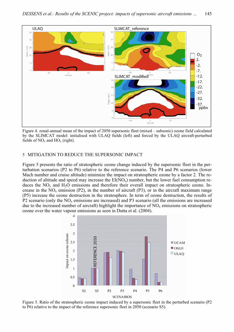
Figure 4. zonal-annual mean of the impact of 2050 supersonic fleet (mixed – subsonic) ozone field calculated by the SLIMCAT model: initialised with ULAQ fields (left) and forced by the ULAQ aircraft-perturbed fields of NOx and HOx (right).

5 MITIGATION TO REDUCE THE SUPERSONIC IMPACT

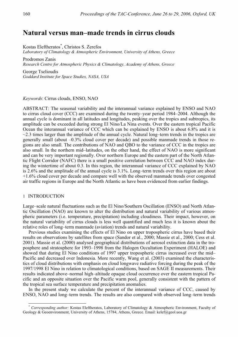
Figure 5 presents the ratio of stratospheric ozone change induced by the supersonic fleet in the per-turbation scenarios (P2 to P6) relative to the reference scenario. The P4 and P6 scenarios (lower Mach number and cruise altitude) minimize the impact on stratospheric ozone by a factor 2. The re-duction of altitude and speed may increase the EI(NOx) number, but the lower fuel consumption re-duces the NOx and H2O emissions and therefore their overall impact on stratospheric ozone. In-crease in the NOx emission (P2), in the number of aircraft (P3), or in the aircraft maximum range (P5) increase the ozone destruction in the stratosphere. In term of ozone destruction, the results of P2 scenario (only the NOx emissions are increased) and P3 scenario (all the emissions are increased due to the increased number of aircraft) highlight the importance of NOx emissions on stratospheric ozone over the water vapour emissions as seen in Dutta et al. (2004).

Figure 5. Ratio of the stratospheric ozone impact induced by a supersonic fleet in the perturbed scenario (P2 to P6) relative to the impact of the reference supersonic fleet in 2050 (scenario S5).


6 CONCLUSION

The impact of supersonic aircraft on the ozone has been quantified for several design of supersonic aircraft or fleet. Some differences can be found between the model reactions to the emissions. The main divergence in the ozone behaviour occurs in the UTLS below 25 km altitude. Above this level, in the middle stratosphere, the response to the emissions from the supersonic aircraft fleet is a reduction of ozone due to the preponderance of the NOx cycle in the ozone destruction cycles at these altitudes. The emissions occur lower in the atmosphere, the strength of this stratospheric ozone reduction is directly related to the strength of the emitted species transported there. The re-duction of ozone in the tropical middle stratosphere can reach 1 to 1.5 % compare to the back-ground for the 2050 fleet. For the direct effect of a supersonic fleet on ozone in the UTLS and mid-dle stratosphere, lowering the cruising altitude of the aircraft (and consequently reducing the Mach number and the fuel consumption) is the best option as seen in the perturbation scenarios.

In the UTLS region it has been proved that the background ratio between the NOx and the HOxspecies are determining the sign of the impact. The more stratospheric character the background atmosphere has, such as found in the OSLO or SLIMCAT model, the more ozone depletion occurs from supersonic emission; but under low NOx, high HOx conditions the ozone chemistry turns to the tropospheric scheme, producing an increase of ozone driven by the local increase of NOx due to the emissions, that happens in the ULAQ simulation. This fact can be reproduced with the UCAM model under the UALQ background conditions for NOx and HOx families.

That last point highlights the importance of the UTLS knowledge to quantify the impact of a su-personic fleet on the atmospheric composition. The position of this cross over point between the production and the destruction of ozone is crucial in order to investigate the impact on the global atmosphere of a supersonic fleet.

REFERENCES

Berntsen T. and I.S.A. Isaksen, 1997: A global 3-D chemical transport model for the troposphere, 1, Model description and CO and Ozone results, Journal of Geophysical Research, vol. 102, , 21.239-21.280.

Chipperfield, M.P., 1999: Multiannual simulations with a three-dimensional chemical transport model, Jour-nal of Geophysical Research, vol. 104, 1781-1805.

Crutzen, P, 1970: The influence of nitrogen oxides on the atmospheric ozone content, Q. J. Roy. Meteorol. Soc., 96, 320-325.

Dutta, M., K. Patten, and D. Wuebbles, 2004: Parametric analysies of potential effects on stratospheric and tropospheric ozone chemistry by a fleet of supersonic business jets projected in a 2020 atmosphere, Na-tional Aeronautics and Space Administration report NASA/CP-2004-213306.

Johnston, H. S., 1971: Reduction of stratospheric ozone by nitrogen oxide catalysts from supersonic trans-port exhaust, Science, vol. 173, 517-522.

Pitari, G., V. Rizi, L. Ricciardulli and G. Visconti, 1993: High speed civil transport impact: role of sulfate, nitric and trihydrate, and ice aerosol studied with a two-dimensional model including aerosol physics,Journal of Geophysical Research, vol. 98, 23141- 23164.

Rogers, H.L., H. Teyssedre, G. Pitari, V. Grewe, P. van Veltoven, and J. Sundet, 2002: Model intercompari-son of the transport of aircraft-like emissions from sub- and supersonic aircraft, Meteorologishe Zeitschrift, vol. 11, 151-159.

Proceedings of the TAC-Conference, June 26 to 29, 2006, Oxford, UK 147

Response in ozone and methane to small emission changes and dependence on cruise altitude

M.O. Köhler*, O. Dessens, H.L. Rogers, O. Wild, J.A. Pyle Centre for Atmospheric Science, Department of Chemistry, University of Cambridge, United Kingdom

Keywords: Aircraft NOX, ozone, methane, UTLS chemistry, cruise altitude, parameterisation

ABSTRACT: Within the scope of the LEEA (Low Emissions Effect Aircraft) project the effects of small changes in aircraft NOX emissions on CH4-NOX-O3 chemistry were systematically investi-gated with the ultimate objective to develop a parametric relationship between the amount / alti-tude / location of emissions and their effect on the climate system. A large number of sensitivity experiments were carried out with the global 3D CTM p-TOMCAT. Aircraft emission data was used from the European AERO2k Global Aviation Emissions Inventory for 2002. In the experi-ments the standard emission profile was altered such that, within discrete cruise altitude bands in the altitude range 5–15 km, emissions were globally increased by 5–20%. Investigation of ozone precursor concentrations, ozone production efficiency and methane lifetime has shown both highly linear and additive behaviour in the atmospheric response to the emission perturbations that were applied. This suggests that in future a linear parameterisation can be used to predict the effects of small emission changes on the chemistry in the UTLS region. The LEEA project was funded by Airbus UK and the Department for Trade and Industry.

1 INTRODUCTION

We have used 3D chemistry transport models to study the impact of aircraft nitrogen oxide (NOX)emissions on ozone (O3) and methane (CH4). Both O3 and CH4 are important greenhouse gases (IPCC, 2001) and changes in their abundance due to aircraft emissions can contribute to climate change (IPCC, 1999). The principal objective of this study was to investigate the atmospheric re-sponse to small perturbations in the emissions as a function of the size of perturbation, cruise alti-tude, and location. The perturbations were applied in form of local scaling of the background emis-sion distribution at different cruise altitude bands. Small increases in emissions could represent the introduction of a new aircraft to the existing commercial fleet or small changes in air traffic de-mand. Of particular interest was the question whether it would be possible to find a parametric rela-tionship between the changes in emissions and the atmospheric composition of ozone and methane. Were such a relationship found, this could then be used to predict the atmospheric impact of future changes within the range of these experiments without the need to conduct costly model experi-ments.

2 MODEL DESCRIPTION

The experiments were carried out using the p-TOMCAT chemistry transport model (O’Connor et al., 2005). This model is an improved and parallelised version of the earlier TOMCAT model (Sav-age et al., 2004) and its gas-phase chemistry scheme focuses on processes relevant to the tropo-sphere and lower stratosphere. For the experiments in this study the vertical resolution was en-hanced to 35 hybrid-pressure levels between 10 hPa and the surface. For each experiment the p-TOMCAT model was integrated for a time period of 2 years and forced by ECMWF operational analyses for the years 2001 and 2002. Aircraft NO2 emission data for 2002 was used from the

* Corresponding author: Marcus Köhler, Department of Chemistry, Lensfield Road, Cambridge, United Kingdom.

Email: [email protected]

148 KÖHLER et al.: Response in ozone and methane to small emission changes and dependence on

European FP5 Project AERO2k (Eyers et al., 2004). A subset of the experiments described below was also carried out by the SLIMCAT chemistry transport model (Chipperfield, 1999) to investi-gate the impact of emission perturbations specifically in the stratosphere. SLIMCAT is forced by UKMO analyses and integrates a stratospheric chemistry scheme on 18 isentropic levels between 335 K and 2700 K (10–55 km). SLIMCAT treats water vapour as a prognostic variable which al-lows for the additional consideration of aircraft H2O emissions and their effects on the stratosphere. A spin-up integration of 6 perpetual years of 2001 meteorology prior to one year of 2002 meteorol-ogy ensured the appropriate representation of transport timescales within the stratosphere.

3 EXPERIMENT DESIGN

The original monthly aircraft emission data, which is provided at 500 ft vertical resolution, was merged to a 1000 ft vertical grid (Eyers et al., 2004) before being included into the models. The al-titude range between 5 and 15 km was subsequently divided into 16 equally spaced cruise altitude bands of 2000 ft (610 m) thickness, from here on referred to as perturbation levels (PL). In a first set of experiments (A) we increased the aircraft emissions locally by 5% for each experiment on one PL at a time. Further experiments (B) with an increase of emissions by 10% and 20% were car-ried out, however only on four selected PLs at approximately 6 km, 7.8 km, 9.5 km, and 11.5 km al-titude. The restriction to these four levels was necessary due to the computational costs associated with each experiment. In a third set of experiments (C) emissions were increased simultaneously by 5% on one of these four PLs from (B) and its neighbouring level underneath, resulting in an emis-sion increase over an altitude band of 4000 ft. Figure 1 shows on the left the zonally and annually integrated AERO2k aircraft emissions in colour. The altitude range covered by the 16 PLs for ex-periment (A) is shaded in light grey, the four principal PLs for experiment (B) and (C) are high-lighted by darker shading. The emission perturbations are applied as a local percentage of emissions in each grid box and therefore the regional distribution of the perturbations reflects the geographical flight routing pattern at the respective cruise altitude band for each PL. Figure 1 shows on the right the horizontal model domain coverage of the perturbations in percent for each PL. Emission pertur-bations below the dashed line (PL 1–11) are located mainly within the troposphere, those above the dashed line (PL 12–16) are located mainly within the stratosphere. The regional coverage of pertur-bations is approximately 60% or more of the horizontal model domain within the troposphere. Within the stratosphere the coverage becomes rapidly smaller with increasing altitude.

Figure 1. Left: AERO2k aircraft emissions for 2002 in kg NO2 per year at 1º 1º 500 ft. Grey shading in-dicates the vertical domain of the perturbation levels, the four perturbation levels of experiment B are high-lighted. Right: Horizontal coverage of the emission perturbation for each perturbation level expressed as a percentage of the model domain. The altitude of the tropopause is shown as a dashed line.

4 IMPACT OF THE GLOBAL AIRCRAFT FLEET ON OZONE AND METHANE

During initial experiments the p-TOMCAT and SLIMCAT models were used to determine the total impact of global air traffic on ozone levels and the lifetime of methane. Both models calculate an increase of ozone in the troposphere and lower stratosphere with a maximum in the northern hemi-

KÖHLER et al.: Response in ozone and methane to small emission changes and dependence on 149

sphere of 6–9 ppbv and a slight ozone decrease in the middle stratosphere. This is in good agree-ment with earlier assessment studies (see e.g. IPCC, 1999; Isaksen et al., 2003; Köhler et al., 2004).A more detailed study of the chemical processes in the p-TOMCAT model shows that net ozone production occurs only above 5 km altitude and exhibits a maximum at approximately 10 km alti-tude where the highest amounts of NOX are emitted. The stratospheric ozone decrease, caused by catalytic destruction following the upward transport of aircraft NOX into the middle stratosphere, is less pronounced in the p-TOMCAT model due to the proximity of its upper boundary at 10 hPa where O3 values are overwritten. Additionally, the timescales of transport of aircraft emissions into the middle stratosphere are represented more appropriately by the SLIMCAT model due to the longer spin-up integration.

An increase in aircraft NOX emissions will lead to an increase in the abundance of hydroxyl radicals (OH), principally through increased O3 formation and by shifting the HOX ratio in favour of OH (Poppe et al., 1993). This increase in OH will lead to CH4 perturbations which in turn influ-ence the abundance of OH in the form of a “feedback” effect as discussed by Fuglestvedt et al. (1999), Karlsdóttir and Isaksen (2000), IPCC (2001) etc. The response time of methane to a change in its abundance is significantly longer than its lifetime (Prather, 1994; 1996) and in order to reach steady state model integrations would have to be carried out over a time scale of decades. Fuglest-vedt et al. (1999) have described a method to calculate the steady state perturbation in CH4 for short model integrations with altered NOX emissions and we adopt their method for this study. In all ex-periments global CH4 levels were kept constant at all times by applying a globally fixed 3-dimensional CH4 reference distribution obtained from a long-term integration (Warwick et al., 2002). The model calculates explicitly the methane loss due to tropospheric OH. Losses due to soil uptake and stratospheric sinks were assumed to have lifetimes of 160 years and 120 years, respec-tively (IPCC, 2001). The feedback factor of 1.30 for the p-TOMCAT model was calculated from the OH perturbation between two reference experiments with normal and with 5% increased meth-ane levels. After steady state in CH4 is reached global aircraft NOX emissions from the AERO2k project have reduced the methane lifetime in the p-TOMCAT model by 2.25% with respect to tro-pospheric OH loss and by 1.88% with respect to all losses. This compares well with values from IPCC (1999) which calculate a reduction of 1.2–1.5% for 1992 and estimate a reduction for 2015 in the range of 1.6–2.9%. This translates into surface mixing ratios being reduced by 44–47 ppbv in the northern hemisphere and by 40–43 ppbv in the southern hemisphere. Moreover, this reduction in methane leads also to a slight decrease in ozone levels (Stevenson et al., 2004), which we assume to be uniformly distributed given the long time scale for steady state to be reached. The ozone bur-den will be reduced by approximately 0.07% (typically 0.1–0.3 ppbv reduction in ozone in the tro-posphere).

Figure 2. Global values of changes in O3 burden (left) and CH4 lifetime (right) due to a 5% emission increase for each perturbation level in experiment A. Values are normalised by the size of the emission perturbation.

5 CRUISE ALTITUDE SENSITIVITY OF EMISSION CHANGES

In experiment (A) emissions were locally increased by 5% on 16 PLs between 5 and 15 km altitude. This is the range where aircraft NOX emissions where found to cause net ozone production and on all perturbation levels the emission increase resulted correspondingly in an increase of the global


ozone burden. Figure 2 (left) shows the global ozone burden change, normalised by the total amount of the emission increase. Between PL 1 and 11 the ozone burden increase becomes larger with increasing altitude of the emission perturbation, with an increasingly larger proportion of the stratospheric ozone burden being perturbed. More detailed investigations showed an increase in ozone production efficiency (Lin et al., 1988) with altitude due to the increasing lifetime of NOX at higher altitudes in the troposphere. Above PL 11 in experiments A.12–A.16 the normalised ozone burden change shows significant variation which is predominantly caused by the change in the re-gional distribution of the background emissions at altitudes above 12 km. At PL 1–11 the distribu-tion of the perturbations covers a comparable geographical region, approximately 60% of the hori-zontal global model domain (Fig. 1). This geographical coverage becomes significantly smaller with increasing altitude for experiments above PL 11 with merely 28% coverage remaining in PL 16. Further test experiments, in which the geographical distribution of the emission perturbations is kept constant above PL 11, have shown that the normalised ozone burden continues to increase with altitude.

The impact of emission perturbations on methane lifetime has a clear dependency on the altitude where the additional NOX is released (Figure 2, right). For perturbations applied within the upper troposphere (PL 8–11) the reduction in CH4 lifetime is largest. Calculations of ozone production ef-ficiency show a local maximum at this altitude range, reflecting the increase of NOX lifetime with altitude within the troposphere. Ozone produced here is transported to lower altitudes where ambi-ent H2O levels are higher, such that the impact on the OH abundance and, hence, the lifetime of CH4 is largest. For emission increases on PL 12–15 the majority of the perturbation is located within the stratosphere. Ozone produced within the lower stratosphere is inhibited from downward transport by the stability above the tropopause, moreover H2O levels in the lower stratosphere are much smaller than in the lower troposphere. Therefore the impact on the CH4 lifetime decreases rapidly when the emission perturbations are located within the stratosphere. On PL 16 the impact on CH4 lifetime becomes larger. This however is an artefact of the geographical location of the emis-sion perturbations. The local emissions increase occurs predominantly at low latitudes and a larger proportion is again released just below the tropical tropopause. Convective activity leads to more effective downward transport of ozone which explains the increased effect on CH4 lifetime.

Figure 3. Changes in the vertical ozone profile near 60º N in p-TOMCAT due to a local emission increase. Emissions were scaled on PL 11 by 5%, 10%, and 20% to investigate linearity (left) and on PLs 10 and 11 to investigate additivity (right).


6 LINEAR AND ADDITIVE RESPONSE TO EMISSION CHANGES

In experiments (B) emissions were increased by 10% and 20% and the changes in ozone were com-pared with those from experiments (A) (5%). Figure 3 (left) shows the change in the vertical ozone profile (zonal average) at 60º N with respect to the reference experiment. The graph shows an en-tirely linear response of ozone levels in the troposphere and lower stratosphere from the surface to approximately 15 km. Above this threshold the lines begin to diverge which is caused by a combi-nation of the length of the model integration and the proximity to the model’s upper boundary. Note that model integrations over two years are likely to be insufficient to represent stratospheric trans-port timescales. Moreover the downward transport of ozone, which is kept at a constant mixing ra-tio at the upper model boundary, prevents the emission perturbation signal from propagating undis-turbed into the middle stratosphere. In the SLIMCAT model, where the integration time was sufficiently long, linearity in the ozone response is diagnosed throughout the stratosphere. This linearity in the ozone response for emission increases between 5–20% was investigated in vertical ozone profile changes at various latitudes and globally on all model levels. At lower latitudes the point of divergence from linearity was found to be at higher altitudes compared with higher lati-tudes, which is attributed to more effective vertical transport of the emissions in the tropics and also to the tropopause being located at higher altitude in this region. It was found that linearity in the ozone response can be assumed with confidence between 60º N and 60º S. At higher latitudes occa-sional outliers of 10% were found, an issue which is still under investigation. In addition to linear scaling of emissions we also investigated whether the atmospheric response is vertically additive with respect to emissions released at different cruise altitude bands (experiment C). Figure 3 (right) shows that the sum of vertical profile changes due to neighbouring perturbation levels is consistent with the profile changes caused with simultaneous emissions perturbations on both levels. Again, this consistency can be seen from the surface to 15 km. At higher altitudes the atmospheric re-sponse is no longer additive for the same reasons described above in the linearity experiments B. The response of the global ozone burden and methane lifetime to local emission scaling on all four altitude bands is shown in Figure 4. It can be clearly seen that the response in both instances is lin-ear with the local scaling of emissions at these altitude bands in the range of 5–20%. Further ex-periments with a local emission increase of 200% at PL 11 have shown that to a first order ap-proximation the ozone burden still responds linearly. This indicates that the CH4-NOX-O3 system may respond linearly to emission increases well beyond 20%. Currently investigations are still in progress as to the extent of the linearity.

Figure 4. Global changes in ozone burden (left) and methane lifetime (right) due to a local increase in aircraft emissions by 5%, 10%, and 20% on perturbation levels 2, 5, 8, and 11.

7 CONCLUSIONS

A large number of sensitivity experiments were carried out with the 3D chemistry transport models p-TOMCAT and SLIMCAT to investigate the effects on atmospheric composition of small pertur-bations to aircraft emissions. The AERO2k Global Emissions Inventory has provided one of the


most realistic emission data sets available to date. The resulting impact of global NOX and H2Oemissions on atmospheric ozone and methane was found to be within the range of results from ear-lier studies, specifically an increase of 6–9 ppbv in O3 in the UTLS region and the reduction of the CH4 lifetime by approximately 2%. With increasing altitude the ozone burden becomes more sensi-tive to changes in aircraft NOX emissions. The largest increase in ozone from subsonic aircraft is found in the northern hemisphere near the tropopause. At the same time NOX emission increases in the upper troposphere were found to result in a particularly strong decrease in the lifetime of meth-ane. The radiative impacts of O3 and CH4 are opposite in sign and work on quite different regional and temporal scales due to their different atmospheric lifetimes. A companion paper by Rädel et al. (this issue) investigates further the radiative aspects of this work.

In further experiments our study has shown that the ozone and methane concentrations respond in both a linear and an additive way to local changes in emissions for the examined perturbation range of 5–20%. This linearity might apply for even larger emission perturbations, an issue which is currently still under investigation. Small inconsistencies seen in the p-TOMCAT results above the tropopause are caused by the proximity of the upper boundary and the insufficient length of the model integration to accurately represent stratospheric processes. SLIMCAT results however showed good linear behaviour also in the stratosphere. The linear relationship established by this study can be used in future work to develop a simplified parameterisation to predict changes in at-mospheric composition caused by small emission changes without the need for costly model ex-periments. As an industrial application this parameterisation could also provide a tool to facilitate the environmental impact assessment of new aircraft during the design phase and help with the characterisation of the environmental performance of existing aircraft.

REFERENCES

Chipperfield, M.P., 1999: Multiannual simulations with a three-dimensional chemical transport model, J. Geophys. Res. 104, 1781–1805.

Eyers, C.J., P. Norman, J. Middel, M. Plohr, S. Michot, K. Atkinson, R.A. Christou, 2004: AERO2k Global Aviation Emissions Inventories for 2002 and 2025. Report number QinetiQ/04/01113, QinetiQ, Farnbor-ough, Hampshire, United Kingdom.

Fuglestvedt, J.S., T.K. Berntsen, I.S.A. Isaksen, H. Mao, X.-Z. Liang, W.-C. Wang, 1999: Climatic Effects of NOX Emissions through Changes in Tropospheric O3 and CH4 – A Global 3-D Model Study, Atmos.Environ. 33, 961-977.

IPCC, 1999: Aviation and the Global Atmosphere. A Special Report of Working Groups I and III of the In-tergovernmental Panel on Climate Change [Penner, J.E., et al. (eds.)] Cambridge University Press, Cam-bridge, United Kingdom, ISBN 0-521-66404-7, 373 pp.

IPCC, 2001: Climate Change 2001: The Scientific Basis. Contribution of Working Group I to the Third As-sessment Report of the Intergovernmental Panel on Climate Change [Houghton, J.T. et al. (eds.)]. Cam-bridge University Press, Cambridge, United Kingdom and New York, NY, USA, ISBN 0-521-01495-6, 881 pp.

Isaksen, I.S.A., R. Sausen, J.A. Pyle, et al., 2003: The EU project TRADEOFF – Aircraft emissions: Contri-butions of various climate compounds to changes in composition and radiative forcing – tradeoff to re-duce atmospheric impact, Project Final Report, Contract No. EVK2-CT-1999-0030, 158 pp. (available from the Department of Geosciences, University of Oslo, Oslo, Norway)

Karlsdóttir, S., I.S.A. Isaksen, 2000: Changing methane lifetime: Possible cause for reduced growth, Geo-phys. Res. Lett. 27, 93–96.

Köhler, M.O., H.L. Rogers, J.A. Pyle, 2004: Modelling the Impact of Subsonic Aircraft Emissions on Ozone: Future Changes and the Impact of Cruise Altitude Perturbations. Proceedings of the European Conference on Aviation, Atmosphere and Climate (AAC), Friedrichshafen, Germany, 30 June – 3 July 2003, in: Airpollution research report 83, European Commission, EUR 21051, pp. 173–177.

Lin, X., M. Trainer, S.C. Liu, 1988: On the Nonlinearity of the Tropospheric Ozone Production, J. Geophys. Res. 93, 15,879–15,888.

O’Connor, F.M., G.D. Carver, N.H. Savage, J.A. Pyle, J. Methven, S.R. Arnold, K. Dewey, J. Kent, 2005: Comparison and visualisation of high-resolution transport modelling with aircraft measurements, Atmos.Sci. Lett. 6, 164–170.

Poppe, D., M. Wallasch, J. Zimmermann, 1993: The Dependence of the Concentration of OH on its Precur-sors under Moderately Polluted Conditions: A Model Study, J. Atmos. Chem. 16, 61–78.


Prather, M.J., 1994: Lifetimes and eigenstates in atmospheric chemistry, Geophys. Res. Lett. 21, 801–804.Prather, M.J., 1996: Time scales in atmospheric chemistry: Theory, GWPs for CH4 and CO, and runaway

growth, Geophys. Res. Lett. 23, 2597–2600.Savage, N.H, K.S. Law, J.A. Pyle, A. Richter, H. Nuss, J.P. Burrows, 2004: Using GOME NO2 satellite data

to examine regional differences in TOMCAT model performance, Atmos. Chem. Phys. 4, 1895–1912.Warwick, N.J., S. Bekki, K.S. Law, E.G. Nisbet, J.A. Pyle, 2002: The impact of meteorology on the interan-

nual growth rate of atmospheric methane, Geophys. Res. Lett. 29, 1947, doi:10.1029/2002GL015282.

154 Proceedings of the TAC-Conference, June 26 to 29, 2006, Oxford, UK

Multi-model Simulations of the Impact of International Shipping on Atmospheric Chemistry and Climate in 2000 and 2030

V. Eyring*, A. Lauer DLR - Institut für Physik der Atmosphäre, Oberpfaffenhofen, 82234 Wessling, Germany

D.S. Stevenson University of Edinburgh, School of GeoSciences, Edinburgh, United Kingdom.

F.J. Dentener European Commission, Joint Research Centre, Institute for Environment and Sustainability, Ispra, Italy.

T. Butler, M.G. Lawrence Max Planck Institute for Chemistry, Mainz, Germany.

W.J. Collins, M. Sanderson Met Office, Exeter, United Kingdom.

K. Ellingsen, M. Gauss, I.S.A. Isaksen University of Oslo, Department of Geosciences, Oslo, Norway.

D.A. Hauglustaine, S. Szopa Laboratoire des Sciences du Climat et de l'Environnement, Gif-sur-Yvette, France.

A. Richter Institute of Environmental Research, University of Bremen, 28359 Bremen, Germany

J.M. Rodriguez, S.E. Strahan Goddard Earth Science & Technology Center (GEST), Maryland, Washington, DC, USA.

K. Sudo, O. Wild Frontier Research Center for Global Change, JAMSTEC, Yokohama, Japan.

T.P.C. van Noije Royal Netherlands Meteorological Institute (KNMI), Atmospheric Composition Research, De Bilt, the Netherlands.

Keywords: international shipping, global modelling, tropospheric ozone, sulphate, radiative forcing

ABSTRACT: The global impact of shipping on atmospheric chemistry and radiative forcing, as well as the associated uncertainties, have been quantified using an ensemble of ten state-of-the-art atmospheric chemistry models and a pre-defined set of emission data. The analysis is performed for present-day conditions (year 2000) and for two future ship emission scenarios. In one scenario emissions stabilize at 2000 levels; in the other emissions increase with a constant annual growth rate of 2.2% up to 2030 (termed the ‘Constant Growth Scenario’). The first key question addressed by this study is how NOx and SO2 emissions from international shipping might influence atmos-pheric chemistry in the next three decades if these emissions increase unabated. The models show future increases in NO2 and ozone burden which scale almost linearly with increases in NOx emis-sion totals. For the same ship emission totals but higher emissions from other sources a slightly smaller response is found. The most pronounced changes in annual mean tropospheric NO2 and sul-phate columns are simulated over the Baltic and North Seas; other significant changes occur over the North Atlantic, the Gulf of Mexico and along the main shipping lane from Europe to Asia, across the Red and Arabian Seas. The second key issue was to examine the range of results given by the individual models compared to the ensemble mean. Uncertainties in the different model ap-

* Corresponding author: Dr. Veronika Eyring, DLR-Institut für Physik der Atmosphäre, Oberpfaffenhofen,

82234 Wessling, Germany. Email: [email protected]

EYRING et al.: Multi-model Simulations of the Impact of International Shipping on Atmos. ... 155

proaches in the simulated ozone contributions from ships are found to be significantly smaller than estimated uncertainties stemming from the ship emission inventory, mainly the ship emission totals, the neglect of ship plume dispersion, and the distribution of the emissions over the globe.

1 INTRODUCTION

Emissions from international shipping contribute significantly to the total budget of anthropogenic emissions from the transportation sector (Eyring et al., 2005) and have been recognized as a grow-ing problem by both policymakers and scientists (Corbett, 2003). Here we use an ensemble of ten state-of-the-art global atmospheric chemistry models to assess the impact of NOx emissions from international shipping on ozone for present-day conditions (year 2000). A subset of four models has been applied to investigate the changes in sulphate distributions due to SO2 emissions from interna-tional shipping. This multi-model approach accounts for intermodel differences and therefore makes the results more robust compared to previous studies based on single models (e.g., Lawrence and Crutzen, 1999; Endresen et al., 2003). In addition, this study for the first time quantifies the po-tential impact of ship emissions in the future (year 2030) for two different future ship emission sce-narios. The participating models have also been evaluated and used in accompanying studies (e.g. Stevenson et al., 2006; Dentener et al., 2006; Shindell et al., 2006, van Noije et al., 2006) as part of the European Union project ACCENT (‘Atmospheric Composition Change: the European NeTwork of excellence’; http://www.accent-network.org). Full details of this study are given in Eyring et al. (2006) and only a brief summary is presented here.

2 MODELS AND MODEL SIMULATIONS

Ten global atmospheric chemistry models have participated in this study. Seven of these models are Chemistry-Transport Models (CTMs) driven by meteorological assimilation fields and three models are atmospheric General Circulation Models (GCMs). Two of the GCMs are driven with the dy-namical fields calculated by the GCM in climatological mode, but the fully coupled mode (interac-tion between changes in radiatively active gases and radiation) has been switched off in the simula-tions of this study. The other GCM runs in nudged mode, where winds and temperature fields are assimilated towards meteorological analyses. Therefore, changes in the chemical fields do not in-fluence the radiation and hence the meteorology in any of the model simulations used here; so for a given model, each scenario is driven by identical meteorology. The main characteristics of the ten models can be found in Table 1 of Eyring et al. (2006) and the models are described in detail in the cited literature.

Two of the five simulations that have been defined as part of the wider PHOTOCOMP-ACCENT-IPCC study have been used in this work: a year 2000 base case (S1) and a year 2030 emissions case (S4) following the IPCC (Intergovernmental Panel on Climate Change) SRES (Spe-cial Report on Emission Scenarios) A2 scenario (Nakicenovic et al., 2000). Full details on the emis-sions used in the S1 and S4 simulations are summarised in Stevenson et al. (2006). To retain consis-tency with all other emissions, ship emissions in the year 2000 (S1) are based on the EDGAR3.2 dataset (Olivier et al., 2001) at a spatial resolution of 1° latitude x 1° longitude. The global distribu-tion of ship emissions in EDGAR3.2 is based on the world’s main shipping routes and traffic inten-sities. EDGAR3.2 includes data for 1995, which have been scaled to 2000 values assuming a growth rate of 1.5%/yr, resulting in annual NOx and SO2 emissions of 3.10 Tg(N) and 3.88 Tg(S), respectively, similar to the emission totals published by Corbett et al. (1999). As noted in Stevenson et al. (2006) in the S4 simulation emissions from ships were included at year 2000 levels by mis-take. All other anthropogenic sources (except biomass burning emissions, which remain fixed at year 2000 levels) vary according to A2 broadly representing a ‘pessimistic’ future situation. The simulation S4 is used in this study to assess the impact of ship emissions under different back-ground levels. An additional model simulation for 2030 (S4s) has been designed to assess the im-pact of shipping if emission growth remains unabated. Ship emissions in S4s are based on a ‘Con-stant Growth Scenario’ in which emission factors are unchanged and emissions increase with an annual growth rate of 2.2% between 2000 and 2030. Vessel traffic distributions are assumed to stay

156 EYRING et al.: Multi-model Simulations of the Impact of International Shipping on Atmos. ...

the same for all model simulations presented here. Full details on the model simulations and model analyses are given in Eyring et al. (2006).

3 RESULTS

For present-day conditions the most pronounced changes in annual mean tropospheric NO2 and SO4columns are found over the Baltic and the North Sea, and also though smaller over the Atlantic, Gulf of Mexico, and along the main shipping lane from Europe to Asia. Maximum near-surface ozone changes due to NOx ship emissions are simulated over the North Atlantic in July (~12 ppbv) in agreement with previously reported results (Lawrence and Crutzen, 1999; Endresen et al., 2003). However, in contrast to Endresen et al. (2003), a decrease in ozone in winter is found over large ar-eas in Europe (~3 ppbv) due to titration (see Figure 1). Overall NOx emissions most effectively pro-duce ozone over the remote ocean, where background NOx levels are small.

Figure 1: Modelled ensemble mean ozone change between (a-c) case S1 (year 2000) and S1w (year 2000 without ship emissions), (d-f) case S4 (year 2030) and S4w (year 2030 without ship emissions), and (g-i) case S4s (year 2030) and S4w. Figure 1a, 1d, and 1g are zonal mean changes (ppbv), Figures 1b, 1e, and 1h are near-surface ozone changes (ppbv) and Figure 1c, 1f, and 1i are tropospheric ozone column changes (DU). From Eyring et al. (2006).

The two 2030 scenarios both specify emissions following the IPCC SRES A2 scenario (Nakiceno-vic et al., 2000). The first future scenario assumes that ship emissions remain constant at 2000 lev-els and under this scenario a slightly smaller response in ozone and sulphate changes due to ship-ping is found compared to the present-day contribution from shipping. This indicates that higher background levels tend to slightly reduce the perturbation from ships. The second emission scenario addresses the question of how NOx and SO2 emissions from international shipping might influence atmospheric chemistry in the next three decades if these emissions grow unabated and one assumes a constant annual growth rate of 2.2% between 2000 and 2030 (‘Constant Growth Scenario’). The models show future increases in NOx and ozone burden which scale almost linearly with increases in NOx emission totals under the same background conditions (see Figure 2).

0 0.1 0.2 0.3 0.4 0.5 0.6 0.7 0.8 0.9 1 1.1 1.2 1.3 1.4 1.5 1.6 1.7 1.8 1.9 2

90S 60S 30S 0 30N 60N 90N1.00.90.80.70.60.50.40.30.2

0.1 (a) S1-S1w Ensemble Mean AZM O3 / ppbv

Hyb

rid v

ertic

al le

vel

-5 -2 -1 0 1 2 3 4 5 6 7 8 9

180 120W 60W 0 60E 120E 18090S60S

30S

EQ

30N

60N

90N (b) S1-S1w Ensemble Mean ANS O3 / ppbv

0 0.15 0.3 0.45 0.6 0.75 0.9 1.05 1.2 1.35 1.5 1.65 1.8

180 120W 60W 0 60E 120E 18090S60S

30S

EQ

30N

60N

90N (c) S1-S1w Ensemble Mean ATC O3 / DU

0 0.1 0.2 0.3 0.4 0.5 0.6 0.7 0.8 0.9 1 1.1 1.2 1.3 1.4 1.5 1.6 1.7 1.8 1.9 2

90S 60S 30S 0 30N 60N 90N1.00.90.80.70.60.50.40.30.2

0.1 (d) S4-S4w Ensemble Mean AZM O3 / ppbv

Hyb

rid v

ertic

al le

vel

-5 -2 -1 0 1 2 3 4 5 6 7 8 9

180 120W 60W 0 60E 120E 18090S60S

30S

EQ

30N

60N

90N (e) S4-S4w Ensemble Mean ANS O3 / ppbv

0 0.15 0.3 0.45 0.6 0.75 0.9 1.05 1.2 1.35 1.5 1.65 1.8

180 120W 60W 0 60E 120E 18090S60S

30S

EQ

30N

60N

90N (f) S4-S4w Ensemble Mean ATC O3 / DU

0 0.1 0.2 0.3 0.4 0.5 0.6 0.7 0.8 0.9 1 1.1 1.2 1.3 1.4 1.5 1.6 1.7 1.8 1.9 2

90S 60S 30S 0 30N 60N 90N1.00.90.80.70.60.50.40.30.2

0.1 (g) S4s-S4w Ensemble Mean AZM O3 / ppbv

Hyb

rid v

ertic

al le

vel

-5 -2 -1 0 1 2 3 4 5 6 7 8 9

180 120W 60W 0 60E 120E 18090S60S

30S

EQ

30N

60N

90N (h) S4s-S4w Ensemble Mean ANS O3 / ppbv

0 0.15 0.3 0.45 0.6 0.75 0.9 1.05 1.2 1.35 1.5 1.65 1.8

180 120W 60W 0 60E 120E 18090S60S

30S

EQ

30N

60N

90N (i) S4s-S4w Ensemble Mean ATC O3 / DU


Figure 2. Global total change in annual mean tropospheric NOx burden (left) and ozone burden (right) due to ship emissions (S4-S4w and S4s-S4w) in each individual model (coloured lines) and the ensemble mean (black line). Inter-model standard deviations are shown as bars. From Eyring et al. (2006).

Therefore, there is evidence that the ship NOx effect is only weakly subject to saturation in its cur-rent magnitude range, and that saturation cannot be expected to help mitigate the effects of near-future increases. In other words a doubling of NOx emissions from ships in the future might lead to a doubling in atmospheric ozone burdens due to ship emissions. In addition, increasing emissions from shipping would significantly counteract the benefits derived from reducing SO2 emissions from all other anthropogenic sources under the A2 scenario over the continents for example in Europe. Under the ‘Constant Growth Scenario’ shipping globally contributes with 3% to increases in ozone burden until 2030 and with 4.5% to increases in sulphate. The results discussed above are calculated under the assumption that all other emissions follow the A2 scenario broadly represent-ing a ‘pessimistic’ future situation. However, if future ground based emissions follow a more strin-gent scenario, the relative importance of ship emissions becomes larger.

Tropospheric ozone forcings due to ships of 9.8 mW/m2 in 2000 and 13.6 mW/m2 in 2030 are simulated by the ensemble mean, with standard deviations of 10-15%. Compared to aviation (~ 20 mW/m2; Sausen et al., 2005) tropospheric ozone forcings from shipping are of the same order in 2000, despite the much higher NOx emissions from ships (Eyring et al., 2005). This can be under-stood because peak changes in ozone due to shipping occur close to the surface, whereas changes in ozone due to aviation peak in the upper troposphere. A rough estimate of RF from shipping CO2suggests 26 mW/m2 in 2000 compared to 23 mW/m2 from aviation CO2. The direct aerosol effect resulting from SO2 ship emissions is approximately -14 mW/m2 in 2000 and decreases to a more negative value of -26 mW/m2 in 2030 under the ‘Constant Growth Scenario’.

We have also investigated the range of results given by the individual models compared to other uncertainties. Uncertainties in the simulated ozone contributions from ships for the different model approaches revealed by the intermodel standard deviations are found to be significantly smaller than estimated uncertainties stemming from the ship emission inventory, mainly the ship emission totals, the neglect of ship plume dispersion, and the distribution of the emissions over the globe. This reflects that the simulated net change from ship emissions under otherwise relatively clean conditions in global models is rather similar and shows that the atmospheric models used here are suitable tools to study these effects.

158 EYRING et al.: Multi-model Simulations of the Impact of International Shipping on Atmos. ...

4 SUMMARY

Maximum contributions from shipping to annual mean near-surface ozone quantified from an en-semble of ten state-of-the-art atmospheric chemistry models and a pre-defined set of emission data are found over the Atlantic (5-6 ppbv in 2000 reaching up to 8 ppbv in the 2030 Constant Growth Scenario). Large increases in tropospheric ozone column are found over the Atlantic and even stronger over the Indian Ocean (1 DU in 2000 and up to 1.8 DU in 2030). Tropospheric ozone forc-ings due to shipping are 9.8 ± 2.0 mW/m2 in 2000 and 13.6 ± 2.3 mW/m2 in 2030. Whilst increasing ozone, ship NOx simultaneously enhances OH, reducing the CH4 lifetime by 0.13 yr in 2000, and by up to 0.17 yr in 2030, introducing a negative radiative forcing. Over Europe, the increase in ship emissions under the ‘Constant Growth Scenario’ will enhance the positive trend in NO2 over land up to 2030. In addition, efforts to lower European sulphate levels through reductions in SO2 emis-sions from anthropogenic sources on land will be partly counteracted by the rise in ship emissions. Globally, shipping contributes with 3% to increases in ozone burden until 2030 and with 4.5% to increases in sulphate. The results discussed above are calculated under the assumption that all other emissions follow the IPCC SRES A2 scenario. However, if future ground based emissions follow a more stringent scenario, the relative importance of ship emissions becomes larger. The range of re-sults given by the individual models compared to other uncertainties has also been investigated. Uncertainties in the simulated ozone contributions from ships for the different model approaches revealed by the intermodel standard deviations are found to be significantly smaller than estimated uncertainties stemming from the ship emission inventory, mainly the ship emission totals, the ne-glect of ship plume dispersion, and the distribution of the emissions over the globe. This reflects that the simulated net change from ship emissions under otherwise relatively clean conditions in global models is rather similar and shows that the atmospheric models used here are suitable tools to study these effects. Full details of this study can be found in Eyring et al. (2006).

ACKNOWLEDGEMENTS

Co-ordination of this study was supported by the European Union project ACCENT (‘Atmospheric Composition Change: the European NeTwork of excellence’. http://www.accent-network.org). The study has also been supported by the Helmholtz-University Young Investigators Group SeaKLIM, which is funded by the German Helmholtz-Gemeinschaft and the Deutsches Zentrum für Luft- und Raumfahrt e.V. (DLR).

REFERENCES

Corbett, J., 2003: New Directions: Designing ship emissions and impacts research to inform both science and policy, Atmospheric Envrionment, 37, 4719-4721.

Corbett, J.J., P.S. Fischbeck, and S.N. Pandis, 1999: Global nitrogen and sulfur inventories for oceangoing ships, J. Geophys. Res., 104(3), 3457-3470.

Dentener, F., D.S. Stevenson, K., Ellingsen, T. van Noije, M. Schultz, et al., 2006: Nitrogen and sulphur deposition on regional and global scales: A multi-model evaluation, Global Biogeochemical Cycles, ac-cepted.

Endresen, Ø., E. Sørgård, J.K. Sundet, S.B. Dalsøren, I.S.A. Isaksen, T.F. Berglen, and G. Gravir, 2003: Emission from international sea transportation and environmental impact, J. Geophys. Res. 108, 4560, doi:10.1029/2002JD002898.

Eyring, V., H.W. Köhler, J. van Aardenne, and A. Lauer, 2005: Emissions from international shipping: 1. The last 50 years, J. Geophys. Res., 110, D17305.

Eyring, V., D.S. Stevenson, A. Lauer, F.J. Dentener, T. Butler, W.J. Collins, K. Ellingsen, M. Gauss, D.A. Hauglustaine, I.S.A. Isaksen, M.G. Lawrence, A. Richter, J.M. Rodriguez, M. Sanderson, S.E. Strahan, K. Sudo, S. Szopa, T.P.C. van Noije, and O. Wild, 2006: Multi-model simulations of the impact of inter-national shipping on atmospheric chemistry and climate in 2000 and 2030, Atmos. Chem. Phys. Dis-cuss., 6, 8553-8604.

Lawrence, M.G., and P.J. Crutzen, 1999: Influence of NOx emissions from ships on tropospheric photochem-istry and climate, Nature, 402, 167-170.


Nakicenovic, N., et al., 2000: IPCC Special Report on Emissions Scenarios, Cambridge University Press, Cambridge, UK, 570 pp.

Olivier, J.G.J., and J.J.M. Berdowski, 2001: Global emissions sources and sinks, in The climate system, ed-ited by J.J.M. Berdowski, R. Guicherit, and B.J. Heij, A.A. Balkema Publishers/Swets & Zeitlinger Pub-lishers, Lisse, the Netherlands.

Sausen, R., I.S.A. Isaksen, V. Grewe, D.A. Hauglustaine, D.S. Lee, G. Myhre, M.O. Köhler, G. Pitari, U. Schumann, F. Stordal, and C. Zerefos, 2005: Aviation radiative forcing in 2000: An update on IPCC (1999), Meteorol. Z., 14, 555-561.

Shindell, D.T., G. Faluvegi, D.S. Stevenson, L.K. Emmons, J.-F. Lamarque, G. Pétron, F.J. Dentener, K. El-lingsen, et al., 2006: Multi-model simulations of carbon monoxide: Comparison with observations and projected near-future changes, J. Geophys. Res., in press.

Stevenson, D.S., F.J. Dentener, M.G. Schultz, K. Ellingsen, T.P.C. van Noije, O. Wild, G. Zeng, et al., 2006: Multimodel ensemble simulations of present-day and near-future tropospheric ozone, J. Geophys. Res., 111, D08301, doi:10.1029/2005JD006338.

van Noije, T.P.C., H.J. Eskes, F.J. Dentener, D.S. Stevenson, K. Ellingsen, M.G. Schultz, O. Wild, et al., 2006: Multi-model ensemble simulations of tropospheric NO2 compared with GOME retrievals for the year 2000, Atmos. Chem. Phys., 6, 2943-2979.

160 Proceedings of the TAC-Conference, June 26 to 29, 2006, Oxford, UK

Natural versus man–made trends in cirrus clouds

Kostas Eleftheratos*, Christos S. Zerefos Laboratory of Climatology & Atmospheric Environment, University of Athens, Greece

Prodromos Zanis Research Centre for Atmospheric Physics & Climatology, Academy of Athens, Greece

George Tselioudis Goddard Institute for Space Studies, NASA, USA

Keywords: Cirrus clouds, ENSO, NAO

ABSTRACT: The seasonal variability and the interannual variance explained by ENSO and NAO to cirrus cloud cover (CCC) are examined during the twenty–year period 1984–2004. Although the annual cycle is dominant in all latitudes and longitudes, peaking over the tropics and subtropics, its amplitude can be exceeded during strong El Nino/La Nina events. Over the eastern tropical Pacific Ocean the interannual variance of CCC which can be explained by ENSO is about 6.8% and it is ~2.3 times larger than the amplitude of the annual cycle. Natural long–term trends in the tropics are generally small (about –0.3% cloud cover per decade) and possible manmade trends in those re-gions are also small. The contributions of NAO and QBO to the variance of CCC in the tropics are also small. In the northern mid–latitudes, on the other hand, the effect of NAO is more significant and can be very important regionally. Over northern Europe and the eastern part of the North Atlan-tic Flight Corridor (NAFC) there is a small positive correlation between CCC and NAO index dur-ing the wintertime of about 0.3. In this region, the interannual variance of CCC explained by NAO is 2.6% and the amplitude of the annual cycle is 3.1%. Long–term trends over this region are about +1.6% cloud cover per decade and compare well with the observed manmade trends over congested air traffic regions in Europe and the North Atlantic as have been evidenced from earlier findings.

1 INTRODUCTION

Large–scale natural fluctuations such as the El Nino/Southern Oscillation (ENSO) and North Atlan-tic Oscillation (NAO) are known to alter the distribution and natural variability of various atmos-pheric parameters (i.e. temperature, precipitation) including cloudiness. Their impact, however, on the natural variability of cirrus clouds is less well quantified and much less it is known about the relative roles of long–term manmade (aviation) trends and natural variability.

Previous studies examining the effects of El Nino on upper tropospheric cirrus have based their results on observations by satellites from space (Sandor et al., 2000; Massie et al., 2000; Cess et al. 2001). Massie et al. (2000) analysed geographical distributions of aerosol extinction data in the tro-posphere and stratosphere for 1993–1998 from the Halogen Occultation Experiment (HALOE) and showed that during El Nino conditions of 1997 upper tropospheric cirrus increased over the mid–Pacific and decreased over Indonesia. More recently, Wang et al. (2003) examined the characteris-tics of cloud distributions with emphasis on cloud longwave radiative forcing during the peak of the 1997/1998 El Nino in relation to climatological conditions, based on SAGE II measurements. Their results indicated above–normal high–altitude opaque cloud occurrence over the eastern tropical Pa-cific and an opposite situation over the Pacific warm pool, generally consistent with the pattern of the tropical sea surface temperature and precipitation anomalies.

In the present study we calculate the percent of the interannual variance of CCC, caused by ENSO, NAO and long–term trends. The results are also compared with observed long–term trends

* Corresponding author: Kostas Eleftheratos, Laboratory of Climatology & Atmospheric Environment, Faculty of

Geology & Geoenvironment, University of Athens, 15784, Athens, Greece. Email: [email protected]

ELEFTHERATOS et al.: Natural versus man-made trends in cirrus clouds 161

in CCC over congested air traffic regions in Europe and the North Atlantic (Zerefos et al., 2003; Stordal et al., 2005; Stubenrauch and Schumann, 2005) to evaluate the significance of the anthro-pogenic (aviation) effect with respect to the natural variability.

2 DATA SOURCES AND METHODOLOGY

The cloud dataset analyzed in this study was produced by the International Satellite Cloud Clima-tology Project (ISCCP) (Rossow and Schiffer, 1999) and covers the period 1984–2004. Cirrus clouds are defined as those with optical thickness less than 3.6 and cloud top pressure less than 440 mb. In order to avoid artificial satellite cloud retrievals after the Mt. Pinatubo eruption in 1991 (Luo et al., 2002) cirrus cloud data taken in 1991 and 1992 were not used in our analysis.

The effect of ENSO on cirrus clouds has been examined by linear regression analysis between monthly mean CCC and Southern Oscillation Index (SOI) in the examined 21–years period. The occurrence of decadal–scale changes in cloud frequency in the tropics (Wang et al., 2002) could af-fect our correlation analysis if they were not taken into account. In order to avoid possible effects from decadal changes in cloud occurrence in the tropics, we first removed from cirrus coverage variability related to the seasonal cycle and long–term trends for the period 1984–2004 based on the following regression model:

( , ) ( , ) ( , )CCC i j S i j T i j residuals (1)

Where i denotes the month and j is the year of CCC and its components, i.e., the seasonal (S) and the long–term trend (T). CCC data were deseasonalized by subtracting the long–term monthly mean (1984–2004) pertaining to the same calendar month. The residuals from Equation (1) were used as input for the correlation analysis between the anomalies of CCC and SOI. The correlation between CCC and NAO index has been computed for the winter–months (December, January and February) over Europe and the North Atlantic.

3 RESULTS AND DISCUSSION

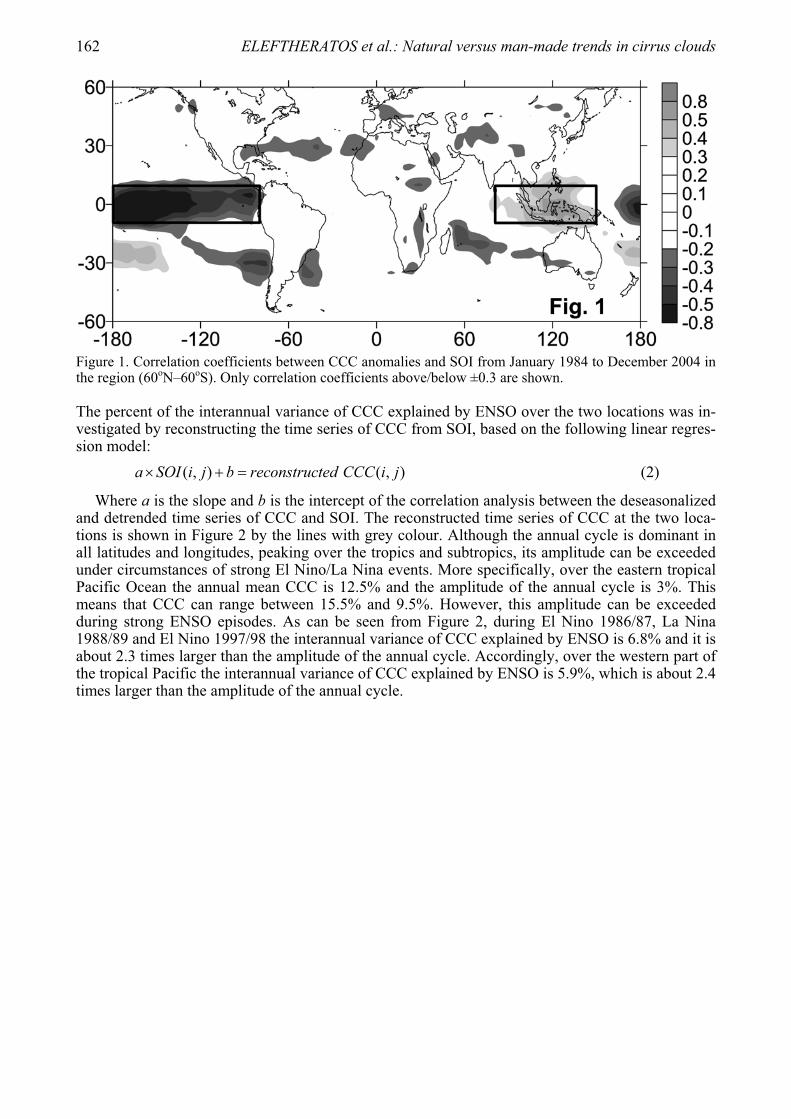
After removing from the time series of cirrus coverage the variability related to the seasonal cycle and long–term trends, ENSO signals become dominant over the eastern and western tropical Pacific Ocean, determining a significant part of the cirrus cloud interannual natural variability. Figure 1 shows the correlation coefficients between the deseasonalized and detrended time series of CCC and SOI from 60oN to 60oS. Negative correlation suggests large amounts of thin cirrus clouds dur-ing warm (El Nino) episodes and positive correlation their absence. More analytically, Figure 2 shows the time series of the anomalies of CCC from 1984 to 2004 versus SOI over (a) the eastern tropical Pacific region (10oS–10oN, 80oW–180oW) and (b) the western tropical Pacific region (10oS–10oN, 80oE–150oE). From Figure 2 it appears that CCC is strongly anti–correlated with SOI over eastern Pacific (R= –0.7) and positively correlated (R= +0.6) over its western part, which prac-tically confirms the correlation map of Figure 1. The two correlation coefficients are statistically significant at the 99% confidence level and suggest that southern oscillation and its associated events (warm and cold) play key roles in the distribution and appearance of thin cirrus clouds over these locations, explaining about one third to half of their large–scale natural variability.

162 ELEFTHERATOS et al.: Natural versus man-made trends in cirrus clouds

Figure 1. Correlation coefficients between CCC anomalies and SOI from January 1984 to December 2004 in the region (60oN–60oS). Only correlation coefficients above/below ±0.3 are shown.

The percent of the interannual variance of CCC explained by ENSO over the two locations was in-vestigated by reconstructing the time series of CCC from SOI, based on the following linear regres-sion model:

( , ) ( , )a SOI i j b reconstructed CCC i j (2)

Where a is the slope and b is the intercept of the correlation analysis between the deseasonalized and detrended time series of CCC and SOI. The reconstructed time series of CCC at the two loca-tions is shown in Figure 2 by the lines with grey colour. Although the annual cycle is dominant in all latitudes and longitudes, peaking over the tropics and subtropics, its amplitude can be exceeded under circumstances of strong El Nino/La Nina events. More specifically, over the eastern tropical Pacific Ocean the annual mean CCC is 12.5% and the amplitude of the annual cycle is 3%. This means that CCC can range between 15.5% and 9.5%. However, this amplitude can be exceeded during strong ENSO episodes. As can be seen from Figure 2, during El Nino 1986/87, La Nina 1988/89 and El Nino 1997/98 the interannual variance of CCC explained by ENSO is 6.8% and it is about 2.3 times larger than the amplitude of the annual cycle. Accordingly, over the western part of the tropical Pacific the interannual variance of CCC explained by ENSO is 5.9%, which is about 2.4 times larger than the amplitude of the annual cycle.


Figure 2. (a) Time series of CCC anomalies from 1984 to 2004 and of SOI over the eastern tropical Pacific (10oS–10oN, 80oW–180oW). (b) Same as (a) but for the western tropical Pacific (10oS–10oN, 80oE–150oE).The lines with grey colour indicate the interannual variance of CCC explained by ENSO (in %).

The other natural oscillation that has been examined as to its effect on CCC is the North Atlantic Oscillation (NAO). As it is known, NAO has two phases; a positive and a negative phase. To study its effect, Figure 3 shows the correlation coefficients between the deseasonalized and detrended time series of CCC and NAO index during the wintertime (December, January and February) in the region bounded by latitudes 15oN–65oN and by longitudes 120oW–80oE. The positive correlations between CCC and NAO index are shown by light grey colours whereas the negative correlations by dark grey colours. The dotted line in Figure 3 bounds the regions where the correlation coefficients are statistically significant at the 95% confidence level (Student’s t–test).

As can be seen from Figure 3, the correlation coefficients of CCC with NAO index consist of negative correlations over regions extending from the eastern part of the North Atlantic to the Mediterranean (up to –0.5 at some locations) and positive correlations over northern Europe and the eastern part of NAFC, explaining part of the cirrus cloud long–term natural variability. Over these regions, the correlation coefficients are statistically significant at the 95% confidence level and compare well with those observed between VV300 and NAO (not shown here). The negative corre-lations over the eastern part of North Atlantic and the Mediterranean (25oN–40oN, 30oW–20oE)could suggest that when the NAO index is positive, CCC is lower than normal in the area, possibly due to enhanced sinking of air masses in the area caused by a stronger than usual high pressure sys-tem at Azores while less frequent west-east advection of moisture and more cold and dry air pene-


trations from north to southeast Europe is taking place. As we move to the north, the correlation co-efficients over northern Europe and the eastern part of NAFC (50oN–65oN, 20oW–10oE) are less statistically significant and cover a smaller area when compared to those between VV300 and NAO (not shown here). Possibly, this could be explained by the fact that during the wintertime there are limited satellite cloud observations by ISCCP over 57o, and in that case our correlation results over 57o are likely to be underestimated. However, it should be considered that other factors i.e. existence of complicated weather conditions and high natural cloud variability during the winter-time in the area may also mask this issue.

Figure 3. Correlation coefficients between CCC anomalies from 1984 to 2004 and NAO index during the wintertime (December, January and February) in the region (15oN–65oN, 120oW–80oE).

Figure 4 shows the time series of the anomalies of CCC from 1984 to 2004 versus NAO index during the wintertime over (a) the eastern part of the North Atlantic and the Mediterranean (25oN–40oN, 30oW–20oE) and (b) northern Europe and the eastern part of NAFC (50oN–65oN, 20oW–10oE). From Figure 4 it appears that CCC is anti–correlated with NAO index over the eastern part of the North Atlantic and the Mediterranean (R= –0.5, significant at the 95% confidence level) and positively correlated over northern Europe and the eastern part of NAFC (R= +0.3, significant at the 90% confidence level), confirming the correlation results of Figure 3.

As in the case of ENSO, we also calculated the percent of the interannual variance of CCC ex-plained by NAO over the two regions by reconstructing the time series of CCC from NAO index based on Equation (2). The reconstructed time series of CCC at the two locations is shown in Figure 4 by the lines with grey colour. More specifically, over the eastern part of the North Atlantic and the Mediterranean (25oN–40oN, 30oW–20oE) the amplitude of the annual cycle of CCC is 3.6% and the interannual variance of CCC explained by NAO is up to 2.4%. Accordingly, over northern Europe and the eastern part of NAFC (50oN–65oN, 20oW–10oE) the interannual variance of CCC explained by NAO is up to 2.6% and it is also smaller than the amplitude of the annual cycle (3.1% cloud cover). Therefore, in northern mid–latitudes the percent of the interannual variance of CCC explained by NAO does not exceed the amplitude of the annual cycle.

Furthermore, to evaluate the significance of the anthropogenic (aviation) effect with respect to the natural variability we have compared our results with manmade long–term trends over Europe and the NAFC as evidenced from earlier studies (Zerefos et al., 2003; Stordal et al., 2005; Stuben-rauch and Schumann, 2005). According to Sausen et al. (1998), at altitude levels around 300 hPa regions that are susceptible to the formation of contrails are located more in the extra–tropics than over the tropics. Over Europe and the NAFC, flight frequencies and flight consumption are high (shown, for example, in Fig. 1 of Zerefos et al., 2003) and situations favourable for contrail forma-tion have been estimated to occur about 7% over Europe and 5% over the NAFC (Stubenrauch and Schumann, 2005). Therefore, over Europe and the NAFC it is possible that cirrus amounts may also include persistent contrails and therefore the cirrus trends can be explained not only by natural long–term variability, but also by variability in manmade cirrus contrails. According to our find-


ings, long–term CCC trends in the region (50oN–65oN, 20oW–10oE) are about +1.6% per decade. These positive trends are statistically significant at the 95% confidence level and compare well with the observed positive manmade trends in cirrus clouds over congested air traffic regions in Europe and the North Atlantic (Zerefos et al 2003; Stordal et al., 2005; Stubenrauch and Schumann, 2005).

Figure 4. (a) Time series of CCC anomalies and NAO index from 1984 to 2004 during the wintertime (De-cember, January and February) over the eastern part of the North Atlantic and the Mediterranean (25oN–40oN, 30oW–20oE). (b) Same as (a) but for northern Europe and the eastern part of NAFC (50oN–65oN,20oW–10oE).The lines with grey colour indicate the interannual variance of CCC explained by NAO (in %).

4 CONCLUSIONS

This study analysed globally cirrus cloud data from ISCCP D2 1984–2004 dataset and calculated the percent of the interannual variance of CCC explained by ENSO, NAO and QBO. The major findings and conclusions can be summarized as follows:

The variability of cirrus clouds is different over different geographical regions and originates from different causes. Although the annual cycle is dominant in all latitudes and longitudes, peak-ing over the tropics and subtropics, its amplitude is exceeded during strong El Nino/La Nina events. Over the eastern tropical Pacific Ocean (10oN–10oS, 80oW–180oW) the annual mean CCC is 12.5% and the amplitude of the annual cycle is 3%. However during ENSO, the interannual variance of CCC explained by ENSO is 6.8% and it is about 2.3 times larger than the amplitude of the annual cycle at these regions. The effects of NAO and QBO on natural cirrus cloudiness in the tropics were


found to be small. Natural long–term trends in CCC in the tropics and subtropics are generally small (between –0.3% and –0.7% per decade) excluding the south extra tropics where no trends have been observed. Possible manmade trends in the tropics are small.

In the northern mid–latitudes, on the other hand, the effect of NAO is more significant and can be very important regionally. More specifically, over the region bounded by latitudes 25oN–40oNand by longitudes 30oW–20oE (eastern part of the North Atlantic and the Mediterranean) cirrus clouds are negatively correlated with NAO index during the wintertime by about –0.5. Over the re-gion between 50oN–65oN and 20oW–10oE (northern Europe and the eastern part of NAFC) the cor-relation is positive (+0.3). Over northern Europe and the eastern part of NAFC the percent of the in-terannual variance of CCC which is explained by NAO is ~2.6% and it is smaller than the amplitude of the annual cycle (3.1% cloud cover). QBO and ENSO were not found to be signifi-cantly correlated with variations in cirrus clouds in the northern mid–latitudes. The general trends in large–scale CCC over the northern mid–latitudes are according to ISCCP negative (–0.4% per decade).

In the region (50oN–65oN, 20oW–10oE) (northern Europe and the eastern part of NAFC) cirrus clouds may also include persistent contrails and therefore cirrus trends in those regions can be ex-plained not only by natural long–term variability, but also by variability in manmade cirrus con-trails. Over these regions, long–term trends in CCC are about +1.6% per decade and are statistically significant at the 95% confidence level. These trends compare well with the observed positive manmade trends in CCC over congested air traffic regions in Europe and the North Atlantic (Zere-fos et al 2003; Stordal et al., 2005; Stubenrauch and Schumann, 2005).

5 ACKNOWLEDGMENTS

This study was conducted within the FP6 Integrated Project “Quantifying the Climate Impact of Global and European Transport Systems” (QUANTIFY, Contract No 003893–GOCE) and contrib-utes to the ECATS Network of Excellence, both funded by the European Commission.

REFERENCES

Cess, R.D., M. Zhang, P.–H. Wang, and B.A. Wielicki, 2001: Cloud structure anomalies over the tropical Pacific during the 1997/98 El Nino. Geophys. Res. Lett. 28, 4547–4550.

Luo, Z., W.B. Rossow, T. Inoue, and C.J. Stubenrauch, 2002: Did the Eruption of the Mt. Pinatubo Volcano Affect Cirrus Properties?. J. Climate 17, 2806–2820.

Massie, S., P. Lowe, X. Tie, M. Hervig, G. Thomas, and J. Russell III, 2000: Effect of the 1997 El Nino on the distribution of upper tropospheric cirrus. J. Geophys. Res. 105(D18), 22725–22741.

Rossow, W.B., and R.A. Schiffer, 1999: Advances in understanding clouds from ISCCP. Bull. Amer. Meteor. Soc. 80, 2261–2287.

Sandor, B.J., E.J. Jensen, E.M. Stone, W.G. Read, J.W. Waters, and J.L. Mergenthaler, 2000: Upper tropo-spheric humidity and thin cirrus. Geophys. Res. Lett. 27(17), 2645–2648.

Sausen, R., K. Gierens, M. Ponater, and U. Schumann, 1998: A diagnostic study of the global distribution of contrails, part I: present day climate. Theor. Appl. Climatol.61, 127–141.

Stordal, F., G. Myhre, E.J.G. Stordal, W.B. Rossow, D.S. Lee, D.W. Arlander, and T. Svendby, 2005: Is there a trend in cirrus clouds cover due to aircraft traffic?. Atmos. Chem. Phys. 5, 2155–2162.

Stubenrauch, C.J., and U. Schumann, 2005: Impact of air traffic on cirrus coverage. Geophys. Res. Lett. 32,L14813, doi: 10.1029/2005GL022707.

Wang, P. H., P. Minnis, B.A. Wielicki, T. Wong, and L.B. Vann, 2002: Satellite observations of long–term changes in tropical cloud and outgoing longwave radiation from 1985 to 1998. Geophys. Res. Lett. 29,1397, 10.1029/2001GL014264.

Wang, P.–H., P. Minnis, B.A. Wielicki, T. Wong, R.D. Cess, M. Zhang, L.B. Vann, and G.S. Kent, 2003: Characteristics of the 1997/1998 El Nino cloud distributions from SAGE II observations. J. Geophys. Res. 108(D1), 4009, doi:10.1029/2002JD002501.

Zerefos, C.S., K. Eleftheratos, D.S. Balis, P. Zanis, G. Tselioudis, and C. Meleti, 2003: Evidence of impact of aviation on cirrus cloud formation. Atmos. Chem. Phys. 3, 1633–1644.

results of the scenic project: impacts of supersonic

Documents