retail investor sentiment and behavior – an empirical analysis
TRANSCRIPT

Retail Investor Sentiment and Behavior – an Empirical Analysis
Zur Erlangung des akademischen Grades eines Doktors der Wirtschaftswissenschaften
(Dr. rer. pol.)
von der Fakultät für
Wirtschaftswissenschaften des Karlsruher Instituts für Technologie
genehmigte
DISSERTATION
von Dipl.-Inform.Wirt Matthias Burghardt
Tag der mündlichen Prüfung: 12. Mai 2010 Referent: Prof. Dr. Christof Weinhardt Korreferentin: Prof. Dr. Marliese Uhrig-Homburg
2010 Karlsruhe

Acknowledgements
I am indebted to many people for their support throughout the preparation of this thesis. In particular, I am grateful to my advisor Prof. Dr. Christof Weinhardt who gave me his support and advice while granting me the freedom to explore different ways to combine academic rigor and practical relevance in interdisciplinary research.
In addition, I would like to thank Prof. Dr. Marliese Uhrig-Homburg for co-advising this thesis. My thanks also go to Prof. Dr. Ute Werner and Prof. Dr. Ingrid Ott for serving on the board of examiners.
I would like to thank my colleagues from the research group Information and Market Engineering at the Institute of Information Systems and Management (IISM) for many fruitful discussions and their valuable comments. I am grateful to Dr. Henner Gimpel who was always ready to discuss problems with me and to share his ideas how to solve them. I also thank Dr. Stefan Seifert for his advice on the direction of this work. Many thanks also go to Dr. Ryan Riordan for being my co-author on many papers and for providing me with encouragement and support. Ryan Riordan and Martin Wagener deserve special thanks for proofreading major parts of the thesis and for providing me with constructive comments.
Parts of this research have been done while I enjoyed the hospitality of London Business School. I am grateful to Prof. Bruce Weber who made this possible.
Finally, I would like to express my gratitude to Oliver Hans, Dr. Christoph Mura, and Christoph Lammersdorf for their constant support while I was research fellow at Boerse Stuttgart. This work would not have been possible without their commitment and dedication to this project.
Matthias Burghardt

Table of Contents ii
Table of Contents
Abbreviations ................................................................................................ v
List of Figures ............................................................................................. vii
List of Tables .............................................................................................. viii
1 Introduction ............................................................................................ 1 1.1. Motivation .......................................................................................................... 1 1.2. Research Outline ................................................................................................ 3 1.3. Overview and Structure ...................................................................................... 7 1.4. Related Publications ........................................................................................... 8
2 Related Theoretical and Empirical Work ............................................. 10 2.1. Introduction to Behavioral Finance .................................................................. 10
2.1.1. Are Financial Markets Efficient? .............................................................. 10 2.1.2. Challenges to Efficient Markets ............................................................... 12 2.1.3. Emergence of Behavioral Finance ............................................................ 14
2.2. Theoretical Work ............................................................................................. 17 2.3. Empirical Work ................................................................................................ 21
2.3.1. Noise Traders ............................................................................................ 21 2.3.2. Investor Sentiment .................................................................................... 22 2.3.3. Individual Investors .................................................................................. 23 2.3.4. Correlated Trading .................................................................................... 23
2.4. Discussion ........................................................................................................ 25 2.4.1. Behavioral Finance ................................................................................... 25 2.4.2. Correlated Trading .................................................................................... 26 2.4.3. Return Correlation .................................................................................... 30 2.4.4. Market Efficiency ..................................................................................... 33
2.5. Conclusion ........................................................................................................ 34
3 Investor Sentiment Construction .......................................................... 36 3.1. Classification of Sentiment Measures .............................................................. 36
3.1.1. Related Work ............................................................................................ 36 3.1.2. Advantages and Disadvantages ................................................................ 38
3.2. Sentiment Measures in Research ..................................................................... 39 3.2.1. The Closed-End Funds Discount .............................................................. 39 3.2.2. Meta-Measures .......................................................................................... 42

Table of Contents iii
3.3. Sentiment Measures in Practice ....................................................................... 45 3.3.1. Survey-based Measures ............................................................................ 45 3.3.2. Market-data-based Measures .................................................................... 52 3.3.3. Meta-Measures .......................................................................................... 56 3.3.4. Summary Statistics ................................................................................... 57
3.4. Evaluation of Sentiment Measures ................................................................... 59 3.4.1. Direct Sentiment Measures ....................................................................... 59 3.4.2. Indirect Sentiment Measures .................................................................... 61 3.4.3. Direct vs. Indirect Sentiment Measures .................................................... 63 3.4.4. Sentiment Measures vs. Market Returns .................................................. 66 3.4.5. Review of Results ..................................................................................... 69
3.5. Conclusion ........................................................................................................ 69
4 Construction of the Euwax Sentiment Index ....................................... 71 4.1. Introduction ...................................................................................................... 71
4.1.1. Securitized Derivatives ............................................................................. 71 4.1.2. European Warrant Exchange .................................................................... 75 4.1.3. Key Facts .................................................................................................. 75
4.2. Data Set ............................................................................................................ 76 4.3. Basic Index Calculation ................................................................................... 79 4.4. Sentiment Analysis ........................................................................................... 82
4.4.1. Number vs. Volume Based Measures ....................................................... 82 4.4.2. Product Types ........................................................................................... 85 4.4.3. Order Types .............................................................................................. 86 4.4.4. Order Volume Groups .............................................................................. 86 4.4.5. Submitted Orders ...................................................................................... 87 4.4.6. Leverage .................................................................................................... 88
4.5. Comparison with other Sentiment Measures ................................................... 89 4.5.1. Indirect Sentiment Measures .................................................................... 90 4.5.2. Direct Sentiment Measures ....................................................................... 92 4.5.3. Review of Results ..................................................................................... 95
4.6. Conclusion ........................................................................................................ 95
5 Retail Investor Herding ........................................................................ 97 5.1. Introduction ...................................................................................................... 97 5.2. Related Work ................................................................................................... 98
5.2.1. Definitions of Herding .............................................................................. 98 5.2.2. Empirical Findings .................................................................................... 99 5.2.3. Discussion ............................................................................................... 102
5.3. Evidence of Market-wide Herding ................................................................. 104 5.3.1. Data ......................................................................................................... 104 5.3.2. Herding Measure Construction ............................................................... 104 5.3.3. Results ..................................................................................................... 106 5.3.4. Review of Results ................................................................................... 109

Table of Contents iv
5.4. Market-wide herding on a broker level .......................................................... 109 5.4.1. Data ......................................................................................................... 110 5.4.2. Results ..................................................................................................... 111 5.4.3. Review of Results ................................................................................... 113
5.5. Stock-Level Herding ...................................................................................... 114 5.5.1. Data ......................................................................................................... 114 5.5.2. Herding Measure ..................................................................................... 116 5.5.3. Results ..................................................................................................... 118 5.5.4. Review of Results ................................................................................... 120
5.6. Conclusion ...................................................................................................... 121
6 The Predictive Power of Retail Investor Sentiment ........................... 123 6.1. Related Work ................................................................................................. 124 6.2. Data and Methodology ................................................................................... 127
6.2.1. Data Set ................................................................................................... 127 6.2.2. Methodology ........................................................................................... 128
6.3. Results ............................................................................................................ 129 6.3.1. Pre- and Post Portfolio Formation Returns ............................................. 129 6.3.2. Control Variables .................................................................................... 134 6.3.3. Portfolio Holding Returns ....................................................................... 140
6.4. Robustness Checks ......................................................................................... 143 6.5. Conclusion ...................................................................................................... 147
7 Conclusion and Future Work ............................................................. 148 7.1. Conclusion ...................................................................................................... 148 7.2. Summary of Contributions ............................................................................. 152 7.3. Future Work ................................................................................................... 154
Appendices ................................................................................................... ix A Appendix to Chapter 4 ...................................................................................... ix
Bibliography ................................................................................................. xi

Abbreviations v
Abbreviations AAII American Association of Individual Investors ADV/DEC Advances/Declines Ratio ADV-DEC Advances minus Declines ASX Australian Stock Exchange CAUD Consolidated Equity Audit Trail Data CBOE Chicago Board Options Exchange CCI Consumer Confidence Index CEFA Closed-End Funds Association CEFD Closed-End Funds Discount CEFD Closed-End Funds Discount col. column DAX Deutscher Aktienindex DJIA Dow Jones Industrial Average e.g. for example EMH Efficient Markets Hypothesis et al. et alii EUWAX European Warrant Exchange G-Mind German Market Indicator i.e. that is ICE Index of Consumer Expectations ICS Index of Consumer Sentiment II Investors’ Intelligence IPO Initial Public Offering ISE International Securities Exchange ISSM Institute for the Study of Security Markets LSV Lakonishok, Shleifer, and Vishny (1992) MSH Morgan Stanley High-Tech Index NASDAQ National Association of Securities Dealers Automated
Quotations NAV net asset value NYSE New York Stock Exchange p/c put/call ratio REX Rentenindex S&P Standard & Poor’s SMH Signed Market Level Herding TAQ Trade and Quote database TRIN Traders Index U.S. United States

Abbreviations vi
UBS Union Bank of Switzerland UMH Unsigned Market Level Herding VAR Vector autoregression VDAX Volatility DAX VIX Volatility Index VWD volume-weighted discount index ZEW Zentrum für Europäische Wirtschaftsforschung

List of Figures vii
List of Figures Figure 1.1: Thesis Structure .............................................................................................. 7 Figure 3.1: CEFD History of Tri-Continental Corp. ...................................................... 42 Figure 3.2: Baker and Wurgler (2006) composite sentiment .......................................... 44 Figure 3.3: Sentix private investors sentiment ................................................................ 46 Figure 3.4: Cognitrend Bull Bear Index ......................................................................... 47 Figure 3.5: AAII Sentiment Index .................................................................................. 48 Figure 3.6: Michigan Consumer Sentiment .................................................................... 49 Figure 3.7: Consumer Confidence Index ........................................................................ 50 Figure 3.8: UBS/Gallup Index of Investor Optimism ..................................................... 51 Figure 3.9: G-Mind ......................................................................................................... 52 Figure 3.10: CBOE put/call ratios .................................................................................. 53 Figure 3.11: VDAX-New ............................................................................................... 54 Figure 3.12: ISEE Sentiment Index ................................................................................ 55 Figure 3.13: Investors’ Intelligence Bearish Sentiment Index ....................................... 57 Figure 4.1: Euwax Sentiment Index (2004 – 2008) ........................................................ 80 Figure 5.1: Pairwise broker correlation ........................................................................ 112 Figure 6.1: Portfolio holding returns ............................................................................ 141 Figure 6.2: Portfolio holding returns by market capitalization ..................................... 142 Figure 6.3: Portfolio holding returns for small caps ..................................................... 143

List of Tables viii
List of Tables Table 2.1: Overview of empirical work on trading imbalances ..................................... 27 Table 2.2: Evidence of return correlation found in empirical work ............................... 31 Table 3.1: Summary statistics of sentiment measures .................................................... 58 Table 3.2: Correlation of weekly and monthly sentiment measures ............................... 60 Table 3.3: Correlation of daily indirect sentiment measures .......................................... 62 Table 3.4: Correlation between indirect and direct weekly sentiment measures ............ 63 Table 3.5: Correlation between indirect and direct monthly sentiment measures .......... 65 Table 3.6: Correlation of sentiment measures and market returns ................................. 67 Table 4.1: Summary statistics ......................................................................................... 77 Table 4.2: Multivariate regression results for order volume .......................................... 84 Table 4.3: Multivariate regression results for order number .......................................... 85 Table 4.4: Leverage ........................................................................................................ 89 Table 4.5: Daily sentiment correlation ........................................................................... 91 Table 4.6: Weekly sentiment correlation ........................................................................ 93 Table 4.7: Monthly sentiment correlation ....................................................................... 94 Table 5.1: Signed and unsigned market herding measures ........................................... 106 Table 5.2: Signed and unsigned market herding measures by market period .............. 108 Table 5.3: Daily herding measures on a broker level ................................................... 110 Table 5.4: Daily herding measures by broker type ....................................................... 111 Table 5.5: Correlation between broker types ................................................................ 113 Table 5.6: Summary statistics by geographical origin of company .............................. 115 Table 5.7: Summary statistics on market capitalization ............................................... 116 Table 5.8: Modified LSV herding measure by product and order type ........................ 118 Table 5.9: Modified LSV herding measure by firm size .............................................. 119 Table 5.10: Comparison of LSV measures across studies ............................................ 121 Table 6.1: Return statistics by product type ................................................................. 130 Table 6.2: Return statistics by order and product type ................................................. 132 Table 6.3: Return statistics for submitted orders .......................................................... 134 Table 6.4: Controlling for market returns ..................................................................... 135 Table 6.5: Controlling for momentum .......................................................................... 136 Table 6.6: Controlling for market capitalization .......................................................... 138 Table 6.7: Portfolio holding return statistics ................................................................ 139 Table 6.8: Annual portfolio holding returns ................................................................. 146 Table A.1: Summary statistics on executed order volume .............................................. ix Table A.2: Summary statistics on submitted orders ......................................................... x

Introduction 1
1 Introduction
“It has long been market folklore that the best time to buy stocks is when individual investors are bearish, and the best time to sell is when individual investors are bullish.”
Robert Neal and Simon Wheatley (1998), p.523
This citation by Robert Neal and Simon Wheatley from their 1998 article about investor sentiment offers several insights and paves the way for this first chapter by making the following statements: First, the opinion of individual investors on the market is important. Second, they are often wrong. Third, individual investor sentiment may support market timing decisions. Fourth, none of the above is scientifically proven.
In this chapter, research about retail investor sentiment in general and the research questions addressed in this thesis in particular are motivated. In addition, the structure of the work as well as the main contributions and related publications are presented.
1.1. Motivation The financial crisis of the year 2008 has lead retail investors to increase their trading activities. As the Financial Times reported, “US retail investors have been trading stocks and options at record levels in recent months, apparently responding to the financial crisis by taking greater control of their own investments”1. The reason for this increased level of trading activity is likely that retail investors want to “take more direct control of their investing, and make decisions themselves about how to rebalance their accounts”.
Retail investor trading has become more and more important for financial institutions, especially during times of crisis: Retail investor orders can provide liquidity to financial institutions and represent a relatively constant source of income for order flow providers.
However, retail investors are often regarded as the “dumb money”2, meaning that their reallocations reduce their wealth on average. The actions of retail investors often serve as contrary indicators in the sense that trading against these indicators would result in profit opportunities. In research, however, no unanimous conclusion has been reached
1 Deborah Brewster, “Retail investors trading at record levels”, Financial Times, November 4, 2008 2 see e.g. Frazzini and Lamont (2008), p. 300

Introduction 2
yet. In recent years, several research articles3 have been published indicating that certain groups of retail investors could be right in their trading decisions, and that their trading could serve as a positive indicator.
Apart from whether retail investors represent the “dumb money” or the “smart money”, the fact that trading by retail investors is correlated is equally important. If retail investors trade in concert, their price impact on the market can be much larger than if they traded independently. Therefore, it is important for market participants to assess retail investor trading and understand their trading behavior.
Retail investor trading is largely driven by sentiment. As opposed to institutional trading which usually relies on professional analyses, tools, and expert opinions, retail investors are said to trade on noise, i.e. information that is not based on fundamental facts but on historical information, or especially attention-grabbing news. In particular, retail investors are especially prone to biases and usually make the same mistakes.
Now, the question is no longer whether retail investor sentiment is important, but rather how to measure investor sentiment correctly. In research and practice, lots of sentiment indicators have been developed or recognized as such. These indicators are usually based on different methodologies, have different underlying data sets, target different retail investors, and are used for different purposes. As of today, there is no universal measure of investor sentiment that is agreed-upon by academics and practitioners, and there is strong doubt that one indicator will establish as a generally accepted sentiment measure because all measures have distinct advantages and disadvantages.
In this work, a unique data set from the European Warrant Exchange at Boerse Stuttgart provides the opportunity to construct a new sentiment indicator and test its properties. Rather than analyzing historical time series of established sentiment indicators, it is possible to isolate the effects of certain orders, products, or brokers and therefore provide new insight on the topic while avoiding the disadvantages of other measures.
Using the sentiment indicator developed in this work, it is shown that retail investors trade in a correlated way and that their trading exhibits strong signs of herding behavior. The sentiment index, constructed from retail order flow data in leverage certificates, exhibits a large negative correlation to the market indicating that the retail investors represented by the sentiment indicator are on average contrarian investors. Finally, a trading strategy developed using the sentiment index is able to generate abnormal returns.
3 see e.g. Jackson (2003), Dorn, Huberman, and Sengmueller (2008), Barber, Odean, and Zhu (2009a), Kaniel, Saar, and Titman (2008)

Introduction 3
1.2. Research Outline The Efficient Markets Hypothesis (EMH) has been the central theory in finance for the last 40 years (Fama 1970). Since its inception, academics have tried to challenge the EMH on many grounds. In particular, its theoretical assumptions about the behavior of individual investors are frequently called into question: First, the rationality of investors, second, the irrelevance of irrational investors, and third, perfectly working arbitrage.
The search for contradicting evidence which has started in the 1980s (e.g. Grossman and Stiglitz (1980) on the impossibility of informationally efficient markets) has consequently led to the emergence of a new field of research – behavioral finance. This field aims to integrate insights from psychology with neo-classical economic theory and rests on two major assumptions: Limited arbitrage and investor sentiment.
Investor sentiment is therefore one of the pillars of behavioral finance. It is defined as the theory of how individuals form their beliefs about the market and future securities prices. In the real world, investors make decisions not only based on simple facts and obvious information but also – and very often – on the basis of their gut-feeling, of comments and opinions of other investors, and psychological traits. Retail investors are often regarded as so-called noise traders: They trade on noise as if it were information, and thereby introduce inefficiency into the trading process. Knowing how investor sentiment is formed and what factors influence investor sentiment is important for academics as well as practitioners to assess market efficiency.
However, measurement of sentiment is difficult: In research as well as practice, many investor sentiment indicators exist that aim to accurately measure investor sentiment. There are different methods of measurement and consequently different outcomes that all have distinctive advantages and disadvantages. This leads to the first research question of this thesis:
Research Question 1:
How can investor sentiment be measured and how are different sentiment indicators related?
The first part of the question warrants an enumeration and a classification of existing sentiment measures in research and practice. The answer to the second part involves an analysis how sentiment measures can be evaluated and compared with each other, and how they are related to other market parameters such as returns and volatility.
As the results show, each of the sentiment measure categories has its advantages and disadvantages. Survey-based measures, on the one hand, have the disadvantage that

Introduction 4
they are costly to generate (an infrastructure is needed with a sufficient participant base which must be constantly maintained), that they can’t be collected as frequent as market data based measures, and finally that people not always do what they say, and that sentiment measures therefore do not express real investor sentiment. Market data based measures, on the other hand, require a theory relating them to investor sentiment – and therefore their interpretation is more difficult.
When asked – while I was research assistant at Boerse Stuttgart – to help creating a measure of retail investor sentiment, I instantly thought of an order imbalance measure based on all retail investor orders submitted to Boerse Stuttgart, in particular to EUWAX, the market segment for securitized derivatives.
In research, measures that are based on order imbalances often have serious problems: Sometimes, measures do not distinguish between buy and sell orders because the data set they are based on does not allow a classification of investor types. Therefore, there must be a sell order for each buy order, and an order imbalance measure can only be created by distinguishing which order initiated the trade. This is often done by an algorithm which does not lead to an exact classification of orders. But there is another problem: Many existing measures do not focus on retail investors alone but include all orders executed on an exchange, such as the NYSE or NASDAQ. In order to separate retail order flow from the rest, trade size classifications or a focus on small firm stocks are used assuming that retail investors rather trade small sizes or small stocks, respectively. However, in today’s times of algorithmic trading, trade sizes continue to decrease, and a separation of retail from institutional order flow becomes more and more difficult.
Imbalance measures that accurately distinguish between retail and institutional orders have other probable drawbacks: Retail investors usually do not have the possibility to sell stocks short to express negative sentiment. Due to this asymmetry of positive and negative sentiment expression, any measure based on such data would be biased.
The most recent academic literature about order imbalance measures mentions other possible problems for the interpretation of investor sentiment: A common result found in many related articles is that retail investors follow a contrarian strategy, i.e. they buy when stocks have decreased in value, and they sell when stock prices have risen. However, this negative correlation could possibly be the result of the automatic execution of stale limit orders in the order book – without retail investors’ intervention. Therefore, a distinction between limit and market orders is important. Another solution to this problem – without the necessity to distinguish limit and market orders – is the use of the order submission time, regardless of whether the order is actually executed at some point in the future.

Introduction 5
The task at Boerse Stuttgart therefore provided me with the opportunity to construct a retail sentiment index with data that has not been used by any researcher before, and at the same time to avoid known problems and shortcomings of existing sentiment measures. Consequently, the second research question involves developing the index and analyzing its properties.
Research Question 2:
Can an index be created from retail order flow data to describe investor sentiment?
This research question actually consists of two parts: First, appropriate data has to be collected and the index has to be calculated. The second part of the question warrants an analysis what properties a good sentiment index should have. It turns out that this is not an easy answer.
It can be argued that since investor sentiment incorporates investors’ expectations and opinions about the market, sentiment measures and market returns should be correlated. In addition, a measure that is based on retail investor orders in index certificates should have a strong relation to market returns. Apart from market returns, the sentiment index should also have relations to other sentiment indexes since they may all pick up the same sentiment signals.
In the course of constructing the index, it is possible to determine the influence of certain parameters on the result, e.g. the difference between an order based measure and a volume based measure, the distinction of different product types, volume groups, order types, and option leverage. Finally, the data set allows to investigate the use of submitted orders for index construction rather than executed orders.
The data used to construct the Euwax Sentiment Index can be used to assess the behavior of retail investors. One of the most important questions in light of behavioral finance research is whether the trading of retail investors is correlated. If this is supported by the data, one of the assumptions of the EMH is seriously challenged, namely that noise traders’ actions cancel each other out. However, if retail investors have the same opinion about market conditions and their trades are correlated, they may actually influence market prices.
Often, the term herding is used to describe a behavior that involves that retail investors buy (sell) simultaneously the same assets as others buy (sell). In research, there is no universally accepted definition of herding, and the term is used for different behaviors and different groups of investors. The first academic article about herding involves parallel trading by institutional investors (Kraus and Stoll 1972), and in the

Introduction 6
development of this strand of research, most of the work is concerned with professional behavior (e.g. the behavior of fund managers).
The availability of retail investor data and the construction of a single measure of retail investor sentiment warrant the analysis whether retail investors exhibit herding behavior which leads to the third research question.
Research Question 3:
Do retail investors herd?
Regardless of whether the retail investors at Boerse Stuttgart are representative of the whole population of retail investors, the analysis of their herding behavior is nevertheless interesting: Retail investors’ trades are possibly correlated and their behavior is based on similar decision making activities.
Answering this research question involves two parts: First, market-wide herding must be investigated, i.e. the phenomenon that retail investors have the same opinion about the market at the same time. Second, stock-level herding is to be analyzed, i.e. the tendency of retail investors to invest in the same underlyings at the same time. This analysis can also be used to compare the findings with related herding literature.
The evidence of correlated behavior among retail investors further supports the assumption that retail investors’ trades influence asset prices. As a natural consequence, the question to ask is whether a sentiment indicator reflecting retail investor sentiment is of any use for other investors.
Apart from the fact that knowing what other investors do may give individuals some affirmation regarding their own investment decisions, it has still to be established whether investors could use the sentiment indicator as a trading signal – either for imitating the other investors’ trades or positioning themselves against them. This leads to the last and maybe most important research question of this thesis.
Research Question 4:
Does sentiment predict returns?
There are many attempts and methodologies that can be used to get an answer to this question. To analyze whether a sentiment indicator can be used to generate abnormal returns, a portfolio construction methodology is employed similar to those used in related literature4. Such a portfolio construction methodology has the advantage that historical data is used to simulate the returns of a trading strategy, and that only extreme
4 see e.g. Kaniel, Saar, and Titman (2008) or Dorn, Huberman, and Sengmueller (2008)

Introduction 7
sentiment readings are used to determine the assets that should be included in the portfolios.
The use of the Euwax data set makes it possible to disentangle effects caused by different product or order types, and investigate the use of submitted orders in index construction.
To get meaningful results, factors such as market returns, momentum, and market capitalization must be controlled for. In fact, a distinction by market capitalization of the underlying companies is necessary to control for the “small minus big” effect. In addition, the separate treatment of large and small cap firms is warranted by related behavioral finance research which indicates that noise traders have the biggest influence on stocks which are difficult to arbitrage and which most probably get their attention – both assumptions lead to small firms.
1.3. Overview and Structure The thesis is structured as depicted in Figure 1.1 below.
Figure 1.1: Thesis Structure
Chapter 1 motivates the research, develops the research questions, and presents an overview and the structure of the thesis as well as related publications.
Chapter 1:Introduction
Chapter 2:Related Theoretical and Empirical Work
Chapter 3:Investor Sentiment
Construction
Chapter 4:Construction of the Euwax
Sentiment Index
Chapter 5:Retail Investor Herding
Chapter 6:The Predictive Power of Retail
Investor Sentiment
Chapter 7:Conclusion and Future Work

Introduction 8
Chapter 2 provides an overview of the main ideas of behavioral finance, and the most important theoretical and empirical work. The focus lies on the comparison, reconciliation, and discussion of the empirical findings.
Chapter 3 presents a classification of sentiment measures and an overview of sentiment measures used in research and practice. A particular emphasis lies on the history of the closed-end funds discount because of its importance in the financial literature. In addition, for each of the sentiment measures used in practice, a graphical presentation is shown along with related research and its main findings. Finally, the evaluation of existing sentiment indicators involves the comparison of direct and indirect measures as well as the relation of sentiment measures to market returns.
In Chapter 4, the construction of the Euwax Sentiment Index is described including the description of the unique data set used, a graphical illustration of the index, and a series of multivariate regressions analyzing the different components of retail order flow. In relation to the results of Chapter 3, the new index is compared to existing measures in research and practice.
Chapter 5 is about retail investor herding. Following an overview of herding definitions and empirical findings in the related literature, empirical results regarding retail investor herding are presented in three parts: First, evidence of market-wide herding is presented involving the examination of different market periods. Second, market-wide herding on a broker level is investigated, i.e. whether retail investors at different brokerages show the same herding behavior. Third, retail investor herding on a stock-level is analyzed to relate the findings to existing literature.
In Chapter 6, the trading strategy based on Euwax Sentiment measures is being developed. This strategy consists of buying high sentiment stocks and selling low sentiment stocks resulting in a zero-cost portfolio. The influence of product and order types is being discussed as well as the difference between using executed and submitted orders. Finally, the optimal holding period for this portfolio strategy is determined using historical data for a period of 5 years.
Chapter 7 concludes this thesis, summarizes the key contributions, and briefly outlines avenues of future research.
1.4. Related Publications Parts of this thesis have been published and presented at various academic conferences and workshops.
At the very beginning of my research involving investor sentiment measures, I presented the general idea of creating retail investor sentiment measures for investment

Introduction 9
decision making at the Conference of Group Decision and Negotiation in Montreal, Canada (Burghardt 2007). A much more detailed extended version of this work co-authored by my colleague Ryan Riordan was presented at the Annual Conference of the Northern Finance Association (NFA) in Toronto, Canada, in fall 2007 and at the Campus for Finance Research Conference in Vallendar, Germany, in January 2008.
The retail investor sentiment construction presented in chapter 4 was presented at the 11th Symposium on Finance, Banking, and Insurance in Karlsruhe and at the FinanceCom in Paris, France (Burghardt and Riordan 2009), both held in December 2008.
Finally, a preliminary version of the herding behavior described in chapter 5 was presented at the FMA 2009 European Meeting in Turin, Italy, co-authored by our visiting research fellow Anshu Ankolekar.
The intention of this thesis is to combine this work as well as the relevant related research and present a structured and sound overview of the research involving retail investor sentiment. Furthermore, the relationship between theory and empirical results is discussed with a focus on the empirical data provided by our industry partner Boerse Stuttgart. Finally, avenues for future research are explored.

Related Theoretical and Empirical Work 10
2 Related Theoretical and Empirical Work
“The assumptions of the EMH rule out the possibility of trading systems based only on information that have expected profits or returns in excess of equilibrium expected
profits or returns.”
Eugene F. Fama (1970), p.384
In recent years, many non-arbitrage algorithmic trading systems have been emerged that rely on the idea of trend-following as do many hedge funds. A relatively recent trend, both in financial research and industrial practice, has been the development of increasingly sophisticated automated trading strategies. Fama’s statement from 1970 is obviously opposed to this development – and maybe it should be acknowledged that markets sometimes are not efficient at all.
In this chapter, an overview of the Efficient Markets Hypothesis (EMH) is given together with a summary of its theoretical assumptions. The most important theoretical and empirical challenges are presented in section 2.1 which have eventually led to the emergence of the Behavioral Finance. In section 2.2 and 2.3, related theoretical and empirical work is presented. More detailed discussions of the related work are included in the following chapters when appropriate. Finally, the focus of section 2.4 lies on the comparison, reconciliation, and discussion of the empirical findings. Section 2.5 concludes.
2.1. Introduction to Behavioral Finance
2.1.1. Are Financial Markets Efficient?
The EMH has been the central theory in finance for the last 40 years. In general terms, the theory of efficient markets is concerned with “whether prices at any point in time fully reflect available information” (Fama 1970, p. 383).
Theoretical assumptions of the EMH
The EMH is based on three assumptions about the behavior of individual investors. First, investors are assumed to be rational and hence value securities rationally. Second, if there are investors that do not act fully rational, then the actions of these irrational investors take effect in opposite directions and therefore cancel each other out. Third, if

Related Theoretical and Empirical Work 11
there are actions by irrational investors that take effect in the same direction, there are enough rational arbitrageurs whose actions bring prices back to the fundamental level.
The first assumption means that all investors value each security for its fundamental value by using the net present value of its future cash flows discounted by known risk factors. When new information about future earnings emerges, investors respond to this new information by adjusting their valuation of the company and hence bidding prices up or down. These prices therefore fully reflect all relevant information which is available to all investors.
The second assumption acknowledges that there are investors that do not react rationally to new information. In this case, it is assumed that these investors trade randomly and that their trades are uncorrelated. Therefore, the trades of irrational investors cancel each other out and do not have any effect on the efficiency of the price formation process. Prices of securities remain at their fundamental values.
The third assumption concerns the situation when the trades of irrational investors are correlated and do not cancel each other out. In this case, the effect on prices could be significant and prices would not be at their fundamental values. It is then assumed that there are enough rational arbitrageurs5 in the market that acknowledge the security’s deviation from its fundamental value and bid prices up or down until the price reflects its fundamental value again. An example may clarify how arbitrage works: Suppose that the correlated trades of irrational investors have driven prices up and away from their fundamental values. Rational arbitrageurs acknowledge this situation and (short) sell the overvalued security. Since they do not want to bear any fundamental risk involved with this kind of security, they simultaneously have to buy an essentially similar security or substitute to hedge this risk. The effect of these selling activities by the arbitrageurs is to bring the overvalued security’s price back to their fundamental value.
The EMH, by itself, is not a well-defined and empirically refutable hypothesis. As Lo (1997) puts it, “it is disarmingly simple to state, has far-reaching consequences for academic pursuits and business practice, and yet is surprisingly resilient to empirical proof or refutation.” There is little consensus between the opinions about the EMH held in academia and industry. In academia, the EMH is widely supported and challenged at the same time. In practice, the EMH seems to be ignored by business practices such as stock-picking and technical analysis. However, the EMH is still regarded as one of the most important theories in finance for the last century.
5 Arbitrage is defined as “buying an asset in one market at a lower price and selling an identical asset in another market at a higher price. This is done with no cost or risk” (Ross, Westerfield, Jaffe 2001).

Related Theoretical and Empirical Work 12
Empirical tests of the EMH
Empirical work on the EMH can be divided into three categories depending on the nature of the information of interest: Weak-form tests are concerned with whether historical price sequences contain information that can be used to predict future returns. Semi-strong form tests include all obviously publicly available information while strong-form tests also include private information and test whether individuals with such information are able to use this information to their advantage.
When researchers began to test the various forms of the EMH, they broadly supported the theory. Evidence especially on the weak-form efficiency was entirely supportive. Fama (1965) finds that stock prices follow a random walk, i.e. they are as likely to rise after a previous day’s increase as after a previous day’s decline. Therefore, ‘technical’ trading strategies that incorporate buying recent winners and selling recent losers would not be profitable.
Tests of the semi-strong form of market efficiency usually use event-studies in which particular news events are studied and tested whether prices adjust to this news immediately or over a period of some days. Fama, Fisher, Jensen, and Roll (1969) present one of the first such studies to demonstrate that prices immediately adjust to new information and that there is no trending of prices after the news event. Therefore, investors cannot gain by using this information to predict returns.
The strong-form efficiency has not received such overwhelming empirical attention like the weak and the semi-strong form efficiency. Researchers seldom take the extreme position that it is not possible to make money by trading on inside information – a fact that is supported by insider traders’ illegal trading activities.
2.1.2. Challenges to Efficient Markets
Theoretical challenges to the EMH
Since its inception, academics have tried to challenge the EMH both theoretically and empirically.
One of the most cited arguments against the EMH is that people do not act fully rational and investors seldom follow the passive investment strategies expected of uninformed market participants as suggested by the EMH. There is a large body of literature that shows that investors are generally reluctant to realize their losses (Odean 1998), that they trade too much (Odean 1999), that they hold on to losing stocks and rather sell winning stocks (Shefrin and Statman 1985), and that especially retail investors actually lose money by trading (Barber, Lee, Liu, and Odean 2009).
Deviations from the expected behavior are highly systematic and even predictable. Deviations occur due to a number of reasons: First, individuals usually do not follow the

Related Theoretical and Empirical Work 13
concepts of the von Neumann-Morgenstern rationality theory and rather show preferences first discovered by Kahneman and Tversky (1979) in their prospect theory. For example, many people display loss aversion which means that their utility function for losses must be steeper than for their gains. Second, individuals do not follow the concepts of Bayes’ rule for assessing the probability of a certain situation. For example, they put higher weight on recent events or overestimate events that somehow got their attention. The result is a biased perception of reality. Third, framing effects cause investors make different decisions depending on how a problem is presented to them. The theories of Kyle (1985) and Black (1986) rely on such behavior.
The critique of the previous paragraph is confronted with the assumption of the EMH that the actions of irrational investors take effect in the same direction and therefore cancel each other out. However, the theories by Kahneman and Tversky argue that people deviate in exactly the same way and their actions are highly correlated. Therefore, this line of defense used by the efficient markets theory could not threaten its opponents.
In addition to the rationality argument, there is the argument concerning effective arbitrage. Efficient markets proponents argue that even if individuals are not fully rational and even if their behavior is correlated, then the actions of rational arbitrageurs should bring prices back to fundamental values and markets remain efficient. However, opponents of the EMH argue that arbitrage in many cases is far from being riskless because close substitutes are often missing (Campbell and Kyle 1993). The interest of risk-averse arbitrageurs is then limited and arbitrage is therefore not as effective as assumed by the efficient markets theory.
The argument that both the irrational investors and the rational arbitrageurs face substantial risks alleviates Friedman’s (1953) theory that only the irrational investors would eventually lose too much money and leave the market. Limited arbitrage can increase arbitrageurs’ losses so they do not survive in the long run.
Empirical challenges to the EMH
Empirical tests of the EMH designed to challenge its validity are plentiful. The first articles challenging the EMH empirically were written in the early 1980s but even today researchers try to find arguments against the various forms of the market efficiency hypothesis.
The weak form hypothesis has been subject of many articles trying to prove that there are ways to successfully predict security returns based on past price information. One of the first papers challenging the weak form is that of De Bondt and Thaler (1985) in which they construct stock portfolios of extreme winners and extreme losers over the past three years. They show that the loser portfolios outperform the winner portfolios for the next 5 years indicating that stock prices tend to overreact on average.

Related Theoretical and Empirical Work 14
Another highly regarded finding challenging the weak form efficiency is stock price momentum. Jegadeesh and Titman (1993) find that – in contrast to the long-term trends identified by De Bondt and Thaler – stock prices tend to predict future short-term movements of up to 12 months in the same direction. In finance, stock price momentum has become a widely accepted source of risk and is now included in many risk-return models (Carhart 1997).
The semi-strong form hypothesis has been challenged by a number of empirical findings. In their seminal paper, Rozeff and Kinney (1976) find seasonal patterns in stock returns over a period of more than 70 years. They discovered the so-called ‘January Effect’ which states that the average monthly return for all NYSE stocks in January is 3.5% whereas other months average about 0.5%. Since small firms are overrepresented in an equal-weighted index, this effect is primarily a small firm phenomenon. Since both the month and the size of the firm are known in advance, excess returns should not occur in semi-strong form efficient markets.
Another challenge to the EMH is presented by findings that the market to book ratio of a company can predict future returns. Among others, Fama and French (1992) find that portfolios of companies with high market to book ratios (‘growth firms’) earn lower returns than portfolios of companies with low market to book ratios (‘value firms’). Shleifer (2000) argues that this is a serious challenge to the EMH because stale information obviously helps predict returns and that excess returns are not due to higher risk as conventionally measured. Fama and French (1993), however, interpret both the size and the market to book ratio as risk factors and add them as additional factors to their Three-Factor-Model which has become a standard in the portfolio management industry. This interpretation as additional risk factors saved the validity of the EMH although this is still highly debated among researchers.
Many of the studies intended to challenge the EMH have been questioned on the grounds of data snooping, less attention to transaction costs, or an improper adjustment for risk factors as Fama criticizes. However, the search for disconfirming evidence which has begun in the 1980s as well as the theoretical doubt has eventually led to the creation of a new field of research – behavioral finance.
2.1.3. Emergence of Behavioral Finance
Behavioral Finance is the “study of human fallibility in competitive markets” (Shleifer 2000) and aims to integrate insights from psychology with neo-classical economic theory. It rests on two major assumptions, namely limited arbitrage and the presence of investor sentiment.
The first major foundation of behavioral finance is limited arbitrage. Arbitrage is defined as “the simultaneous purchase and sale of the same, or essentially similar,

Related Theoretical and Empirical Work 15
security in two different markets for advantageously different prices” (Sharpe and Alexander 1990). This means arbitrage is based on the valuation difference between the security and its substitute, i.e. an essentially similar security which possesses the same risk characteristics. In the real-world, however, many securities do not have close substitutes, making arbitrage more difficult if not impossible for rational investors. Moreover, even when good substitutes are available, prices often do not converge to their fundamental prices instantaneously because irrational traders continue to move prices further away. Arbitrageurs then face the risk that they have to liquidate their positions before prices converge to their fundamental values. Due to the short time horizon of arbitrageurs, arbitrage remains risky and is therefore limited resulting in inefficient prices.
The form of this inefficiency is affected by the second major foundation of behavioral finance, investor sentiment. Investor sentiment is the theory of how individuals actually form their beliefs about the market and future securities prices. In the real-world, investors make decisions not only on the basis of simple facts and obvious information but also – and very often – on the basis of their gut-feeling, comments and opinions of other investors, and many more psychological traits. Therefore, it is very important to assess which psychological biases have the greatest influence on decision-making in certain situations. The theory of investor sentiment tries to provide answers to this question.
Noise Trader Risk and Limited Arbitrage
“Noise causes markets to be somewhat inefficient, but often prevents us from taking advantage of inefficiencies.” (Black 1986)
The definition of noise trading was first developed by Fischer Black in his seminal paper “Noise” from 1986 in which he refers to noise as opposed to information. Noise traders are people trading on noise as if it were information. In his definition they cannot expect to earn money from noise trading. He argues that without noise trading there would be very little trading in individual assets (this reasoning is in line with the “no trade theorem” by Milgrom and Stokey (1982)). However, with lots of noise traders in the market, it pays for those with information to trade. In Black’s opinion, noise traders lose money most of the time, while information traders as a group make money.
According to Black (1986), determining whether a trader is a noise trader or an information trader is difficult: Noise trading puts noise in the prices, and information traders cannot be sure whether the information they have has already been reflected in the prices. If it has, then trading on this information is just like trading on noise. As a result, there is a lot of ambiguity on who is an information trader and who is a noise trader.

Related Theoretical and Empirical Work 16
Before the discussion of the importance of noise trading and behavioral finance started in the 1980s, economists like Friedman (1953) and Fama (1965) ignored their influence on price formation because the existence of rational arbitrageurs would drive prices to fundamental values and noise traders out of the market. De Long, Shleifer, Summers, and Waldman (1990) examine these arguments and explicitly focus on the limits of arbitrage exploiting noise traders’ misperceptions.
Arbitrage is a sophisticated form of risk-free speculation. Arbitrageurs – in the presence of noise traders – do bring prices to the fundamental values in line with the Friedman/Fama argument. However, this kind of arbitrage is not riskless: There is the risk that noise traders’ beliefs will not revert to their mean for a long time and might in the meantime become even more extreme. De Long et al. (1990) call this source of risk noise trader risk. If noise traders are, for example, pessimistic about a security, they sell it and therefore drive its price down and below its fundamental value. Rational arbitrageurs buy the security and hope that its price recovers soon. If, however, more noise traders come into the market and continue selling the asset, arbitrageurs may be forced to liquidate their position in order to limit their losses. The fear of this loss limits their original arbitrage position in the first place.
The two main assumptions of limited arbitrage are that arbitrageurs are risk-averse and have reasonably short horizons. Assuming that arbitrageurs are rather risk-averse is intuitive since arbitrage is commonly defined as a riskless transaction. The second assumption about the short horizons of arbitrageurs can be justified by agency arguments: Since most arbitrageurs are assumed to manage not their own money but money from other investors, they are required to report positive results in relatively short periods of time. If a mispricing they have identified takes longer to vanish they may be forced by their investors to liquidate their positions at a loss. Interest payments on borrowed money even increase this problem.
Investor Sentiment
Investor sentiment is the theory of how investors form their beliefs. Barberis, Shleifer, and Vishny (1998) present a formal model which takes both the available empirical evidence as well as the known psychological theories of belief formation into account.
Their theory is based on the empirical observation of both overreaction and underreaction of investors inconsistent with the weak-form and the semi-strong form of the EMH. On the one hand, the underreaction evidence shows that security prices tend to underreact to news announcements: After good news, prices show an upwards trend after the initial price reaction, and after bad news, prices trend downwards indicating that they have not fully adjusted to the news. This phenomenon is also called momentum, i.e. the nature of prices to trend expressed by the positive autocorrelation of returns over relatively short horizons. The overreaction evidence, on the other hand,

Related Theoretical and Empirical Work 17
shows that over longer horizons security prices overreact, especially if there is a longer pattern of the same type of news. The study by De Bondt and Thaler (1985) as mentioned in section 2.1.1 is an example of overreaction: Investors overreact to a series of either good or bad news, and as a result, winners underperform and losers outperform in the following years. Eventually, prices revert to the mean after a period of exaggeration.
The model of Barberis, Shleifer, and Vishny (1998) is based on two main observations in psychology: conservatism and the representativeness heuristic. Conservatism is a phenomenon identified by Edwards (1968) that states that individuals are slow to change their beliefs in the face of new evidence. In particular, their beliefs are changed in the right direction as suggested by the Bayes Theorem but the change is too small in magnitude so that an underreaction to the new evidence is perceived. The second phenomenon is the representativeness heuristic discovered by Tversky and Kahneman (1974). People subject to this heuristic think that they see patterns in truly random sequences. They evaluate the probability of an event by the degree to which it is similar to other e.g. past events although past events may not be representative of future ones. For example, investors affected by this bias might conclude that firms with a consistent history of earning growth rates over the past several years continue to grow at the rate suggested by past earnings. As a consequence, investors disregard the possibility that earnings do not grow into the sky and eventually reverse.
2.2. Theoretical Work In this section, five models involving noise trading or investor sentiment are presented. The purpose of this chapter is therefore to give an overview of the motivation, the structure, and the basic results of the theoretical work that shaped the behavioral finance.
Noise Trader Risk in Financial Markets
The model of De Long et al. (1990) was one of the first models that included noise traders in the calculation of market prices. They introduced the concept of the noise trader risk which has to be borne by arbitrageurs with a short time horizon.
The model is a simple overlapping generations model with two groups of agents: On the one hand, there are risk averse sophisticated investors with rational expectations, and on the other hand, there are noise traders with incorrect beliefs and irrational misperceptions. Agents have the choice between a safe asset with a fixed dividend and perfectly elastic supply, and an unsafe asset with the same fixed dividend but without elastic supply - it is in fixed and unchangeable quantity. Agents live two time periods. They choose their portfolios in the first period to maximize the perceived expected

Related Theoretical and Empirical Work 18
utility given their own beliefs about the mean of the distribution of the price in the second time period. The representative sophisticated investor accurately perceives the distribution of returns from holding the risky asset, and so maximizes expected utility given that distribution. The representative noise trader misperceives the expected price of the risky asset.
Noise traders in the model create an additional risk for all agents. The price of the risky asset depends on the direction and intensity of the next noise trader generation’s misperception. The time horizon for the liquidation of the assets is very short since all agents have to sell their assets to the next generation in the second period.
One of the main contributions of the De Long et al. (1990) model is the interpretation of the rational arbitrageurs’ decisions as a reaction to existing noise traders. In the model, it is rational to take future noise traders’ sentiment into account when deciding about the own portfolio. Eventually, rational arbitrageurs trade not only on fundamental data but also on noise.
A Model of Investor Sentiment
Barberis, Shleifer, and Vishny (1998) present a model of investor sentiment6 which explains phenomena of underreaction to new information as well as overreaction to either good or bad news because people tend to see familiar patterns.
The model incorporates one risk-neutral representative investor and one asset. The beliefs of this representative investor should be regarded as ‘consensus beliefs’ even when real investors’ opinions are different. The investor’s beliefs affect prices and returns.
The earnings of the asset follow a random walk. However, the representative investor believes that the behavior of earnings moves between two states (or regimes): In the first state, earnings are mean-reverting. That means e.g. upward price movements are followed by price declines with a high probability. In the second state, earnings trend, i.e. earnings tend to rise further after an increase and to decline after a drop. The probabilities for the change between two states, i.e. the transition probabilities, are fixed in the investor’s mind. In any given period, the investor thinks that the firm’s earnings are more likely to stay in the state they are in than to change to the other state. The investor then observes earnings and updates his beliefs according to the Bayes’ model. In particular, he raises the likelihood that he is in the trending state if earnings increase in subsequent periods. On the other hand, the likelihood for the mean-reverting state is increased if good and bad earnings alternate.
The model describes an investor who does not know the true state of the world. His decision only depends on the observed results of the very last period. Conservatism 6 This model has already been briefly mentioned in section 2.1.3.

Related Theoretical and Empirical Work 19
leads to a slow reaction to new information. Overreaction to information is caused by the representativeness heuristic when this information follows a series of news with the same sign.
Investor Psychology and Security Market Under- and Overreaction
The model by Daniel, Hirshleifer, and Subrahmanyam (1998) presents a theory of an under- and overreaction of securities markets. It is based on investor overconfidence about the precision of private information on the one hand, and the underestimation of public signals.
In their model, each member of a continuous mass of agents is overconfident in the sense that if he receives a signal, he overestimates its precision. Not all agents, however, receive a signal in each time period. Those agents receiving a signal belong to the group of the informed whereas those who do not receive a signal belong to the group of the uninformed agents. Informed agents are risk neutral and uninformed agents are risk averse.
Each agent is endowed with a securities portfolio at the beginning of the first period (there are three periods in total). At date 0, individuals begin with their endowments and identical prior beliefs. They trade solely for the purpose of optimal risk transfer. At date 1, the group of informed agents receives a noisy private signal about the underlying security value and trades with the uninformed. The informed agents underestimate the variance of the signal. The uninformed agents know that some agents have received a signal, and estimate the variance of this signal correctly. At date 2, a noisy public signal arrives and trading continues. This time, the signal variance is estimated correctly by the informed as well as the uninformed agents. Finally, at date 3, conclusive public information arrives, the security pays a liquidating dividend, and consumption occurs.
The central aspect of the model is that overconfidence regarding the private signal leads to an overreaction of the security’s price to new information. In the long run, this overreaction is partially corrected so a long term price reversal can be explained. Furthermore, overconfidence of the agents leads to higher volatility, especially in period 1 in which the noisy private signal is perceived. In addition, price movements as a result of public information are positively correlated with future price movements.
To incorporate momentum in their model, Daniel, Hirshleifer, and Subrahmanyam (1998) expand their basic model by linking the agents’ confidence to the success of their previous actions. A public signal confirms their choice if it points into the same direction. For example, if an agent buys an asset and later a positive signal confirms his choice, his confidence is strengthened. Therefore, overreaction can occur in periods 1 and 2 and a momentum effect can be observed.

Related Theoretical and Empirical Work 20
A Unified Theory of Underreaction, Momentum Trading, and Overreaction in Asset Markets
Hong and Stein (1999) present a model in which two types of bounded rational traders – momentum traders and news watchers – interact. Effects involving under- and overreaction are not explained by phenomena from psychology but are solely a result of this interaction.
In their basic model, a risky asset is traded in each time period with a fixed dividend in the final time period. News watchers are bounded rational because they can observe only a part of the available information at one point in time. In addition, it is not possible for them to conclude any price information from each other’s actions. Information regarding the final dividend is distributed in independent and non-overlapping parts such that the full information is distributed over several time periods. In contrast to the news watchers, momentum traders have a finite time horizon. They trade with the news watchers who act as competing market makers. Momentum traders follow a positive feedback strategy and solely trade on historic price information. Due to their bounded rationality, they are not capable to obtain a better prediction of the price by more sophisticated models.
The model has the following core contributions: First, the piece-wise distribution of information to the news watchers leads to an initial underreaction to incoming information. Momentum traders who want to profit from this underreaction and follow a positive feedback strategy, thereby cause the momentum effect and as a result an overreaction of the prices. Both under- and overreaction are therefore caused by the slow information diffusion. The model explains an underreaction of market prices in the short run and an overreaction in the long run. Eventually, the overreaction is reversed by the actions of the momentum traders and a correction can be observed.
Hong and Stein (1999) enhance their model by expanding the strategies of the momentum traders to increase the degree of rationality. They are now able to act not only as momentum traders but as contrarians. In addition, they can choose a better model to predict prices and base their decision on several past periods. However, it is shown that the results from the basic model still hold. Even with the addition of a third group of traders – the smart money – Hong and Stein (1999) still explain underreaction, the momentum effect and the resulting overreaction. Only if the smart money accepts infinite risks do prices follow a random walk.
Distinguishing Between Rationales for Short-Horizon Predictability of Stock Returns
The model by Subrahmanyam (2005) is primarily concerned with short-horizon return reversals. He identifies two possible explanations in the literature: Some authors take the position that market microstructure phenomena (e.g. risk-aversion-related inventory effects or the bid-ask bounce) are the causes of these reversals. Other authors suggest

Related Theoretical and Empirical Work 21
that market overreaction and correction (belief reversion) drive the predictability of monthly returns.
Subrahmanyam (2005) presents an equilibrium model that incorporates both risk-aversion-related inventory phenomena as well as behavioral effects. In his model, risk averse agents absorb order flow from outside investors. A risky security is traded at dates 1 and 2, and pays off a random amount at date 3. There is a continuum of risk averse agents who absorb liquidity shocks that appear in the market. At date 2, each agent receives a signal. Part of the agents misassesses the variance of the signal as too low. This captures overreaction and correction in the model. A demand shock arrives at the market on date 2, and risk averse agents demand a premium to absorb it. Therefore, the security price has two components: The liquidity premium and the conditional expectation of the asset’s value.
By capturing agents’ beliefs as well as risk aversion, the model allows to obtain implications for the relation between current returns, past returns, and past order flows. The model indicates that risk-aversion-related inventory effects are accompanied by a relation between current returns and past order flows. However, no such relation can be found with respect to belief reversion. Subrahmanyam (2005) concludes – as other research indicates – that inventory effects do not appear to completely account for the return reversal usually found at a monthly horizon. His results accord with the notion that monthly reversals are caused, in substantial part, by reversals in beliefs of financial market agents.
2.3. Empirical Work This section presents related empirical work regarding noise trading, investor sentiment, individual investors, and correlated trading. The purpose of this section is to give an overview of the important literature along these research fields. A more detailed review of the relevant work can be found in the literature sections of the respective chapters when appropriate.
2.3.1. Noise Traders
Since De Long et al. (1990) have researches tried to measure noise trading activity and investigate its impact on market quality. Often, market sentiment plays an important role in this research.
Brown (1999) argues that if noise traders affect prices and the resulting noise can be interpreted as sentiment causing systematic risk, i.e. additional volatility, then sentiment should be correlated with volatility. Sentiment is measured directly using the AAII Sentiment Survey, and the resulting risk is measured by the volatility of closed-end

Related Theoretical and Empirical Work 22
investment funds. Brown finds that unusual levels of investor sentiment are in fact associated with greater volatility of closed-end investment funds.
Beaumont et al. (2005) propose an integrated framework that jointly tests for the effects of individual as well as institutional sentiment on return and volatility. They use weekly direct measures of sentiment and relate them to stock returns and volatility. They find that individual investor sentiment is a market wide risk factor that does not only affect small cap stocks.
Berkman and Koch (2008) empirically study the influence of noise trading on market liquidity. They use the dispersion in daily net initiated order flow across brokers as a proxy for the level of noise trading in stocks traded at the Australian Stock Exchange (ASX). They find that market liquidity increases with the level of noise trading (i.e. greater trading volume, market depth, higher arrival rate of uninformed investors, lower spreads) and that the sensitivity of stock prices to net initiated order flow decreases in the level of noise trading.
Barber, Odean, and Zhu (2009b) investigate individual investor trading at two large brokers and measure the tendency to buy or sell the same set of stocks. They conclude that the buying and selling behavior of individual investors is systematic and individual investors therefore do have the potential to affect asset prices.
2.3.2. Investor Sentiment
There is a large body of literature that tries to relate measures of investor sentiment to volatility and returns in an attempt to analyze the impact of investor sentiment on asset prices. Most of them use direct measures of sentiment (see Chapter 3 for a more detailed overview).
Lee, Jiang, and Indro (2002) use the Investors’ Intelligence sentiment to test the impact of noise trader risk on the formation of conditional volatility and expected returns. They explicitly jointly test the four behavioral effects as introduced in De Long et al. (1990) and find that shifts in sentiment are negatively correlated with market volatility.
Brown and Cliff (2004) explore the relation between investor sentiment and near-term stock returns in a vector autoregression framework. Although sentiment levels and changes are strongly correlated with contemporaneous market returns, they find that sentiment has little predictive power for near-term future stock returns. In a later article, Brown and Cliff (2005) use the Investors’ Intelligence sentiment to test two hypotheses: First, excessive optimism leads to periods of market overvaluation. Second, high sentiment is followed by low cumulative long-run returns as prices revert to their fundamental level. Both hypotheses are supported by the results, and so Brown and Cliff (2005) – in contrast to their earlier paper – conclude that asset values are affected by investor sentiment.

Related Theoretical and Empirical Work 23
Wang, Keswani, and Taylor (2006) investigate the relationships between sentiment, returns, and volatility. They explicitly test whether sentiment is useful for volatility forecasting purposes. By using different sentiment indicators (e.g. the put/call ratio, the ARMS index and survey measures), they find that most of these measures are caused by returns and volatility rather than vice versa.
Related research is not restricted to stock markets but extends to the futures and options markets as well: Han (2008) uses three sentiment proxies and examines whether they affect prices of the S&P 500 options. He presents evidence that investor sentiment helps explain both the shape of the S&P 500 option volatility smile, and the risk-neutral skewness of the index return extracted from the index option prices. Kurov (2008) uses the AAII and II sentiment measures and relates them to trading in the S&P 500 and Nasdaq E-mini futures markets. They show that index futures traders use positive feedback trading strategies, and that there is a positive relation between investor sentiment and the intensity of positive feedback trading.
2.3.3. Individual Investors
Research on the behavior of individual investors has started in the 1990s with the importance of individual investor trading on asset prices established by the noise trader theories of Black, Kyle, and De Long et al. De Bondt (1998) draws a portrait of the individual investor and reviews prior research.
Recent studies about individual investor behavior include Griffin, Harris, and Topaloglu (2003) who explore the dynamics of institutional and individual trading by classifying trading data for Nasdaq securities as originating from individuals, institutionals, and market makers. Coval, Hirshleifer, and Shumway (2005) analyze the transactions of individual investors at a large discount brokerage and evaluate the investors’ trading performance. They provide evidence that some individual investors are able to persistently beat the market. Dorn and Huberman (2005) link individual investor performance to survey results and find a relation between self-reported risk-aversion and actual portfolio volatility.
Barber, Lee, Liu, and Odean (2005) draw a less positive portrait of the individual investor: Using day trading data from Taiwan they find that the profits of day traders are not sufficient to cover their transaction costs. Only a relatively small group of day traders are actually able to earn consistently strong returns. In a later paper involving the same data set from Taiwan, Barber, Lee, Liu, and Odean (2008) find that virtually all individual trading losses can be traced to their use of aggressive orders.
2.3.4. Correlated Trading
Since the discovery of individual investors in the context of noise trading, researchers have tried to empirically measure the behavior of individual investors. In particular,

Related Theoretical and Empirical Work 24
they have tried to show that individual investors buy and sell stocks in concert and that this behavior has a significant impact on asset prices.
One of the most straightforward methods to measure the behavior of individual investors is the creation of order imbalance measures. Order imbalance measures put the buying and selling of individual investors into proportion and aggregate it to a single ratio which can then be compared to other key indicators such as stock returns or volatility. In particular, order imbalances can signal excessive investor interest in a stock, and if this interest is autocorrelated, then order imbalances could be related to future returns. However, order imbalance measures only work if it is possible to separate a subgroup of investors and measure the order imbalance of this subgroup. Otherwise, there would be the “for every buyer, there’s a seller” argument which would make it impossible to calculate imbalance measures.
Traditionally, volume has provided the link between trading activity and returns in the literature. Chordia, Roll, and Subrahmanyam (2002) (and subsequently Chordia and Subrahmanyam (2004)) are among the first to explore an order imbalance measure and analyze long-term order imbalances on a comprehensive cross-sectional sample of NYSE stocks. Jackson (2003) focuses on retail transactions and creates an order imbalance measure for individual investors in Australia. Kumar and Lee (2006) develop a buy-sell-imbalance measure using retail investor transactions. They are among the first to empirically support a role for investor sentiment in the formation of returns.
Pan and Poteshman (2006) analyze options trading data and construct a put/call ratio from option volume initiated by buyers to open new positions. Their work is unique in that they empirically transfer the concept of information trading in the options market. Andrade, Chang, and Seasholes (2008) examine changes in margin holdings by individual investors on the Taiwan Stock Exchange. They find that weekly changes in margin holdings correlate positively with contemporaneous returns and negatively with returns over subsequent weeks.
More recently, there are several papers analyzing individual investors’ trading behavior by creating order imbalance measures: Dorn, Huberman, and Sengmueller (2008) use the data set of a large German discount broker to construct a herding measure which shows that retail investors tend to be on the same side of the market in a given stock. Schmitz, Glaser, and Weber (2007) also use data of a German discount broker and construct an imbalance measure for warrant investors. Using exchange data on individual investors, Kaniel, Saar, and Titman (2008), Barber, Odean, and Zhu (2009a), and Hvidkjaer (2008) – in contemporaneous research – construct imbalance measures and analyze the dynamic relation between net individual investor trading and short-horizon stock returns. Subrahmanyam (2008) provides a longer-term perspective on lagged order flows and returns by studying a large sample of NYSE stocks and relates it primarily to inventory effects. Boehmer and Wu (2008) use a unique data set from the

Related Theoretical and Empirical Work 25
New York Stock Exchange which enables them to differentiate between order imbalances of institutions, market makers, and individuals.
2.4. Discussion
2.4.1. Behavioral Finance
Behavioral finance as a new research field is as intensely debated as its counterpart, the theory of efficient markets. There are at least as many opponents to the emergence of the behavioral finance as there are critics of the EMH.
Behavioral finance emerged because traditional finance appears to play a limited role in understanding questions especially regarding individual investors, such as a) why individual investors trade, b) how they form their expectations, or c) how they perform. In the consequence, behavioral finance literature has addressed questions such as a) what mistakes to avoid when trading or b) how to develop strategies that generate superior returns (Subrahmanyam 2007).
In general, opponents of the behavioral finance usually offer the same objections: First, behavioral finance is said to create ad-hoc models explaining specific stylized facts and thereby failing to provide a general theory. Second, behavioral finance research is said to be subject to data mining because researchers are focused on finding deviations from traditional finance models. Third, it is claimed that behavioral finance does not present a unified theory (e.g. utility maximization using rational beliefs).
The main reason why the behavioral finance fails to satisfy the requirements of traditional finance researchers is that it is a “positive” theory, i.e. a theory that explains how people behave rather than how people should behave. In contrast, “normative” theories are based on rational economics and concepts whose empirical support appears to be limited. Subrahmanyam (2007) concludes that “the evidence in favor of inefficient financial markets is far more compelling than that in favor of efficient ones” (p. 18).
In contrast, Fama (1998) argues that “market efficiency survives the challenge from the literature on long-term anomalies” (p. 283). He bases his arguments on two observations: First, many of the studies on long-term returns that suggest market inefficiency establish underreaction or overreaction. Fama (1998), however, argues that these anomalies are consistent with market efficiency if they are split randomly between under- and overreaction. In other words, underreaction will be as frequent as overreaction in an efficient market. Second, he finds that the long-term anomalies described in the literature are sensitive to methodology. In particular, they may completely disappear when different statistical approaches are used to measure them or when other models for expected returns are taken into consideration.

Related Theoretical and Empirical Work 26
Fama (1998) also criticizes that the studies challenging market efficiency rarely test a specific alternative to market efficiency. Rather than presenting an alternative theory that can be tested they merely dispute market efficiency. Market efficiency could only be replaced by a better model of price formation that itself would then be potentially rejectable by empirical tests. Fama explicitly acknowledges the work of Barberis, Shleifer, and Vishny (1998) and that of Daniel, Hirshleifer, and Subrahmanyam (1997) because both present rejectable hypotheses. He concludes, however, that the models do well on the anomalies they are designed to explain. But their prediction of long-term reversal would not capture the long-term results observed in the literature. Fama predicts that “we will soon see a menu of behavioral models that can be mixed and matched to explain specific anomalies” (p. 291).
2.4.2. Correlated Trading
Section 2.3 has shown that there is a growing amount of literature about individual investors, their behavior, and especially their correlated trading. Retail investors obviously have an ability to forecast future returns, although the explanation for this finding is still to be explored. Most scholars admit that “some individuals behave foolishly all the time and all individuals behave foolishly some of the time” (Chordia, Roll, Subrahmanyam 2005, p. 272).
This section presents an overview of the empirical research about correlated trading and identifies differences among the respective papers while trying to summarize and reconcile them. Table 2.1 presents an overview of the individual papers and provides summaries of data sources, periods, data frequency, and details how the order imbalance measures are constructed and what kind of data is used for that.

Related Theoretical and Empirical Work 27
Tab
le 2
.1: O
verv
iew
of e
mpi
rica
l wor
k on
trad
ing
imba
lanc
es
This
tabl
e su
mm
ariz
es re
cent
em
piric
al p
aper
s ab
out c
orre
late
d tra
ding
and
trad
ing
imba
lanc
es. D
ata
sour
ces,
perio
ds, a
nd fr
eque
ncy
are
show
n in
col
umns
2 to
4,
Sign
ing
in c
olum
n 5
refe
rs to
how
buy
and
sel
l ord
ers
are
sepa
rate
d, M
easu
re in
col
umn
6 sh
ows
the
mea
sure
s de
velo
ped
in th
e re
spec
tive
pape
rs, T
arge
t gro
up in
co
lum
n 7
com
pare
s diff
eren
t inv
esto
r gro
ups a
s ind
entif
ied
in th
e pa
pers
, and
Ord
er ty
pe in
the
last
col
umn
indi
cate
s whe
ther
diff
eren
t ord
er ty
pes a
re d
istin
guis
hed.
Art
icle
Dat
a so
urce
Perio
dFr
eque
ncy
Sign
ing
Mea
sure
Targ
et g
roup
Ord
er ty
peA
ndra
de, C
hang
, and
Sea
shol
es (2
008)
Taiw
an S
tock
Exc
hang
e19
94-2
002
wee
kly
exac
tch
ange
in sh
ares
held
in
mar
gin a
ccou
nts
indivi
dual
inves
tors
all o
rder
type
s
Barb
er, L
ee, L
iu, a
nd O
dean
(200
5)
Taiw
an S
tock
Exc
hang
e19
95-1
999
daily
exac
ttra
ding
vol
ume
indivi
dual
inves
tors
, day
tra
ders
pass
ive a
nd
aggr
essiv
e or
ders
Barb
er, L
ee, L
iu, a
nd O
dean
(200
8)
Taiw
an S
tock
Exc
hang
e19
95-1
999
daily
exac
ttra
ding
vol
ume
indivi
dual
inves
tors
pass
ive a
nd
aggr
essiv
e or
ders
Barb
er, O
dean
, and
Zhu
(200
9a)
NY
SE, A
mex
, Nas
daq
(ISSM
, TA
Q)
1983
-200
1m
onth
ly, w
eekl
yLe
e an
d Re
ady
num
ber o
f sm
all b
uyer
-ini
tiate
d tra
des
small
ord
ers
mar
ket o
rder
s only
Barb
er, O
dean
, and
Zhu
(200
9b)
two
large
U.S
. disc
ount
and
re
tail b
roke
rs19
91-1
999
mon
thly
exac
tnu
mbe
r of t
rade
sind
ividu
al inv
esto
rsall
ord
er ty
pes
Berk
man
and
Koc
h (2
008)
A
SX19
91-1
994
daily
n/a
tradi
ng v
olum
eall
inve
stors
mar
ket o
rder
s only
Boeh
mer
and
Wu
(200
8)
NY
SE (C
AU
D)
2000
-200
4da
ilyex
act
num
ber o
f tra
nsac
tions
, sh
ares
, and
dol
lars
six a
ccou
nt ty
pes
all o
rder
type
s
Cho
rdia
and
Subr
ahm
anya
m (2
004)
NY
SE (I
SSM
, TA
Q)
1988
-199
8da
ilyLe
e an
d Re
ady
volum
e an
d nu
mbe
r of
trans
actio
nsall
inve
stors
mar
ket o
rder
s only
Cho
rdia,
Rol
l, an
d Su
brah
man
yam
(200
2)
NY
SE (I
SSM
, TA
Q)
1988
-199
8da
ilyLe
e an
d Re
ady
num
ber o
f tra
nsac
tions
, sh
ares
, and
dol
lars
all in
vesto
rsm
arke
t ord
ers o
nly
Dor
n, H
uber
man
, and
Sen
gmue
ller (
2008
) G
erm
an D
iscou
nt B
roke
r19
98-2
000
daily
exac
tnu
mbe
r of s
hare
s tra
ded
indivi
dual
inves
tors
mar
ket a
nd lim
it or
ders
Grif
fin, H
arris
, and
Top
aloglu
(200
3)
Nas
daq
100
2000
-200
1da
ilyex
act
tradi
ng v
olum
ere
tail,
instit
utio
nal,
mar
ket
mak
erall
ord
er ty
pes
Hvid
kjae
r (20
08)
NY
SE, A
mex
, Nas
daq
(ISSM
, TA
Q)
1983
-200
5m
onth
lyLe
e an
d Re
ady
signe
d sm
all tr
ade
turn
over
(S
STT)
small
trad
es b
y siz
e pr
oxy
mar
ket o
rder
s only
Jack
son
(200
3)
ASX
(56
brok
ers)
1991
-200
2w
eekl
yex
act
tradi
ng v
olum
eind
ividu
al inv
esto
rsall
ord
er ty
pes
Kan
iel, S
aar,
and
Titm
an (2
008)
NY
SE (C
AU
D)
2000
-200
3da
ily, w
eekl
yex
act
tradi
ng v
olum
eind
ividu
al inv
esto
rsall
ord
er ty
pes
Kum
ar a
nd L
ee (2
006)
U
.S. d
iscou
nt b
roke
rage
fir
m19
91-1
996
mon
thly
exac
ttra
ding
vol
ume
indivi
dual
inves
tors
all o
rder
type
s
Pan
and
Pote
shm
an (2
006)
C
BOE
1990
-200
1da
ilyex
act
tradi
ng v
olum
efo
ur in
vesto
r clas
ses
all o
rder
type
sSc
hmitz
, Glas
er, a
nd W
eber
(200
7)G
erm
an D
iscou
nt B
roke
r19
97-2
001
daily
exac
tbu
yers
ratio
indivi
dual
inves
tors
all o
rder
type
sSu
brah
man
yam
(200
8)
NY
SE (I
SSM
, TA
Q)
1988
-200
2m
onth
lyLe
e an
d Re
ady
tradi
ng v
olum
eall
inve
stors
mar
ket o
rder
s only

Related Theoretical and Empirical Work 28
There are some crucial differences among the papers concerning the source of the data, its frequency and period, regional focus, target group, and the construction of the imbalance measure.
Data sources
There are several kinds of data sources that are used for individual investor research: First, researchers use proprietary data sets from brokers that reveal customer transactions as well as customer holdings on an anonymous account level. These data sets allow for the analysis of customer profitability, holding periods, and imbalance measures on the basis of individual investors. In particular, imbalance measures such as the percentage of investors that are net buyers (buyers ratio) can be calculated.
Second, proprietary stock exchange data is used including transactions from several different brokers but seldom on an account level. Therefore, measures such as the buyer ratio cannot be calculated. There are exceptions such as the Taiwan Stock Exchange whose data reveals transactions on an individual investor level. For this reason, researchers such as Andrade, Chang, and Seasholes (2008) and Barber, Lee, Liu, and Odean (2009) have made extensive studies in this market. Boehmer and Wu (2008) and Kaniel, Saar, and Titman (2008) both use the proprietary Consolidated Equity Audit Trail Data (CAUD) provided by the New York Stock Exchange that includes information whether the order originates from an institution or an individual.
Third, publicly available exchange data can be used to infer order imbalance measures. This methodology is the least reliable methodology but is used by several authors due to the availability of the data. It has some drawbacks: The sign of the trade has to be inferred in order to distinguish aggressive from passive orders. Usually, the Lee and Ready (1991) algorithm is used to sign transactions. In addition, if the target is the individual investor, trades have to be sorted by trade size to distinguish the different investor groups such as individual investors and institutionals.
Signing
Five of the articles mentioned in Table 2.1 use the Lee and Ready (1991) algorithm to identify the side of the trade. Rather than distinguishing orders by order type or investor group, order imbalances are defined in terms of order aggressiveness. Based on this algorithm, a trade executed at a price higher than the prevailing quote midpoint is classified as buyer-initiated. If the transaction price equals the quote midpoint, it is classified as buyer-initiated if the transaction price is above the previous transaction price. Seller-initiated orders are defined analogously.
This signing procedure seeks to identify the active side of the trade which is willing to pay a premium over the quote midpoint. In practice, aggressive orders are likely to be market orders or marketable limit orders whereas passive orders are usually limit orders

Related Theoretical and Empirical Work 29
or market maker orders. Order imbalances based on this algorithm count only the initiating side of the trade and, therefore, provide a measure of the relative impatience of buyers and sellers.
The correctness of the Lee and Ready (1991) algorithm, however, is controversial: Lee and Radhakrishna (2000) show that 40% of NYSE trades cannot be classified at all, and 7% of the remaining trades are not classified correctly. On the other hand, Barber, Odean, and Zhu (2009a) find that order imbalance measures based on buyer- and seller-initiated small trades from the TAQ/ISSM data base correlate well with order imbalance measures based on trades of individual investors from proprietary brokerage data. They conclude that small trades signed by the Lee and Ready (1991) algorithm are reasonable proxies for the trades of individual investors.
Whether the signing algorithm leads to a reasonable measure of order imbalance or whether an exact classification should be preferred – fact is that these different methodologies probably lead to different results which have to be interpreted as such.
Regional differences
There are certainly differences among the behaviors of individual investors in different parts of the world. For example, individual investors in Taiwan may show a totally different behavior than investors in Germany or the USA. Therefore, inferences about the behavior of individual investors must always be made in light of the investment culture of the country or region where the data is collected from.
Period and frequency
Data period and frequency differs throughout the related research. In most of the papers a daily frequency is used though some authors present results on a monthly basis. This is not only due to the availability of the data but also to the specific research focus, i.e. whether long-term or short-term anomalies are to be investigated.
It is therefore important to judge any differences in the conclusions in light of the data frequency. For example, both Barber, Odean, and Zhu (2009a) and Hvidkjaer (2008) use the same data and a similar imbalance measure but come to different conclusions regarding short-term return predictability. In a reconciliation, however, Barber, Hvidkjaer, Odean, and Zhu (2006) show that their short-term results are not necessarily contradictory when the data frequency is harmonized.
Order Types
Another important difference among previous research is the differentiation between market and limit orders. All papers using the Lee and Ready (1991) algorithm only include market orders by assumption whereas all other papers may include limit orders as well.

Related Theoretical and Empirical Work 30
Dorn, Huberman, and Sengmueller (2008) are among the first to distinguish market and limit orders and get different results depending on the order type. Their data set from the discount broker allows them to determine the order type exactly and differentiate even further between speculative and non-speculative orders. Barber, Lee, Liu, and Odean (2009) differentiate between passive and aggressive orders due to their unique data set from the Taiwan Stock Exchange. Investors in Taiwan are not allowed to submit market orders, so an executed limit order must be identified as marketable or non-marketable.
In recent research, Linnainmaa (2009) finds that trading patterns such as the disposition effect or contrarian behavior can be explained in large part by investors’ use of limit orders. He argues that these pattern arise mechanically because limit orders are price-contingent and suffer from adverse selection. Besides, the differentiation between market and limit orders has not received a lot of attention in the related literature although Dorn, Huberman, and Sengmueller (2008) show that this differentiation is important. In addition, research on submitted rather than executed orders is missing – a gap that we would like to fill with our work.
Order Imbalance Measure Calculation
Although an order imbalance measure is being developed in all papers, authors have done it in different ways: Some researchers report trading volume imbalance, some report imbalances based on the number of trades or the number of stocks traded. In some papers, an imbalance measure based on the number of buyers as opposed to all traders is calculated.
Given the many differences among all empirical papers, there is no doubt that their results and conclusions differ as well. The main questions are whether order imbalance measures are correlated with contemporaneous and future return data.
2.4.3. Return Correlation
Contemporaneous returns
Empirical results regarding a contemporaneous correlation of order imbalances and stock returns are mixed. Among the papers that report a positive contemporaneous correlation are Chordia, Roll, and Subrahmanyam (2002), Chordia and Subrahmanyam (2004), Dorn, Huberman, and Sengmueller (2008), Andrade, Chang, and Seasholes (2008), Hvidkjaer (2008), and Barber, Odean, and Zhu (2009a). In general, their work suggests that periods of intense buying correlates with rising stock prices, i.e. investors are positive feedback traders and buy when prices go up.
In contrast, Griffin, Harris, and Topaloglu (2003), Jackson (2003), Kumar and Lee (2006), Kaniel, Saar, and Titman (2008), and Boehmer and Wu (2008) report a strong

Related Theoretical and Empirical Work 31
negative correlation between order imbalances and stock returns. Their work suggests that individuals are negative feedback traders and buy when prices decline and sell when prices go up. Table 2.2 summarizes the findings regarding contemporaneous and subsequent correlation of order imbalances and returns.
Table 2.2: Evidence of return correlation found in empirical work
This table presents a summary of findings on return correlation found in recent empirical work. Frequency is reported to explain differences in subsequent columns. The column Contemporaneous correlation shows whether returns and order imbalance measures are negatively or positively (or not at all) correlated. The column Forecasting power indicates whether the authors have found any return forecasting ability of their measures. The last column (Duration) reports the duration of return predictability.
It is not straightforward to reconcile the results. Boehmer and Wu (2008) as well as Griffin, Harris, and Topaloglu (2003) find that order flow and prices have a high contemporaneous correlation but that signs differ for individuals and institutions. According to their results, order flow of individuals is negatively correlated to stock returns whereas order flow of institutions is positively correlated to stock returns suggesting that individuals provide liquidity to actively investing institutions. This reasoning complements the results in Kaniel, Saar, and Titman (2008) as well as Jackson (2003) whose results support the existence of very strong negative feedback trading at the individual stock level by small investors.
On the contrary, both Chordia, Roll, and Subrahmanyam (2002), and Chordia and Subrahmanyam (2004) report a positive contemporaneous correlation, i.e. excess buy orders drive up prices and excess sell orders drive down prices. However, they do not
Article Frequency Contemporaneous correlation
Forecasting power
Duration
Boehmer and Wu (2008) daily negative (individuals); positive (institutions)
positive up to 4 days
Chordia and Subrahmanyam (2004) daily positive positive one dayChordia, Roll, and Subrahmanyam (2002) daily positive negativeDorn, Huberman, and Sengmueller (2008) daily positive positive up to 2 daysGriffin, Harris, and Topaloglu (2003) daily negative (individuals);
positive (institutions)none --
Pan and Poteshman (2006) daily -- positive up to 3 weeksSchmitz, Glaser, and Weber (2007) daily -- positive up to 2 daysJackson (2003) weekly negative positive up to 2 weeksKaniel, Saar, and Titman (2008) weekly negative positive up to 4 weeksAndrade, Chang, and Seasholes (2008) weekly positive negative up to 10 weeksBarber, Odean, and Zhu (2009a) weekly positive positive up to 4 weeksHvidkjaer (2008) monthly positive negative up to 2 yearsKumar and Lee (2006) monthly negative positive one monthSubrahmanyam (2008) monthly -- negative up to 2 months

Related Theoretical and Empirical Work 32
differentiate between individual and institutional investors – an omission that could very well lead to these results.
The remaining papers summarized in Table 2.2 also report a positive correlation but a missing differentiation between individual and institutional investors cannot be found because all of them focus on individual investors’ data. However, their methods defining individual investors’ trades differ: Barber, Odean, and Zhu (2009a) and Hvidkjaer (2008) use small trades as proxies for small individual investors’ trades. It is possible that their measure includes different trades than e.g. Boehmer and Wu’s (2008) measure that provides an exact differentiation between all investor groups.
Andrade, Chang, and Seasholes (2008) acknowledge that their results differ from those reported in Kaniel, Saar, and Titman (2008). They argue that the results reported by Kaniel, Saar, and Titman (2008) are possibly driven by the execution of stale limit orders (on average) which causes the U.S. investors to trade against price movements whereas the data used in their study, by contrast, are placed by active Taiwanese investors who demand liquidity. Therefore, differences between investor behaviors across countries could explain the results.
Dorn, Huberman, and Sengmueller (2008) report a positive contemporaneous correlation. They argue that the negative correlations between limit order imbalances and contemporaneous returns found by other researchers are due to the strong mechanical relation between price movements and limit order execution. They do things differently, in that they only use speculative market orders by individual investors. Order imbalances on these orders are positively correlated to contemporaneous returns which they explain with serially correlated price pressure.
Subsequent returns
In the case of subsequent return correlations, the related work is apparently not consistent either. Four papers find that order imbalances are negatively related to future returns, i.e. periods of intense buying are followed by subsequent returns reversals suggesting that retail investors’ behavior is suboptimal. One paper does not find a significant correlation of order imbalances and future stock returns. All others, i.e. the majority of the related literature in Table 2.2, find a significant positive correlation of order imbalance and subsequent stock returns differing in the observation frequency and the duration of the observed effect.
It is easier to reconcile the seemingly contrarian results, especially after the work by Barber, Odean, Zhu, and Hvidkjaer (2006) who find that their earlier contrarian findings are easily reconciled when using the same data frequency. They find that both papers document strong reversals at long horizons (e.g. one year) and strong continuations at short horizons (e.g. one week). In this light, the negative correlations documented by Hvidkjaer (2008) as well as Subrahmanyam (2008) are due to their monthly frequency.

Related Theoretical and Empirical Work 33
When changing the frequency from monthly to weekly, results in Hvidkjaer (2008) equal those of Barber, Odean, and Zhu (2009a) which is likely to be the case with the data in Subrahmanyam (2008) as well.
Griffin, Harris, and Topaloglu (2003) do not find any forecasting power in their data. This might be due to their relatively short data set, and the missing differentiation concerning market capitalization or order type.
The results by Chordia, Roll, and Subrahmanyam (2002) suggest a negative correlation as well. In their later paper (Chordia and Subrahmanyam 2004) they find the opposite pattern regarding future returns. However, they explain the difference by the focus on market-wide order imbalances on the one hand, and order imbalances at the individual stock level on the other hand.
The negative correlation found by Andrade, Chang, and Seasholes (2008) does not seem to fit among all other results. Again, maybe the Taiwanese investors show a very different behavior than those in Europe, Australia, and the United States. Lee, Liu, Roll, and Subrahmanyam (2004) support this reasoning and find that all trader classes act as market makers and that they are quite successful in doing it. This suggests that the behavior of individual investors in Taiwan can be quite different from other markets in which market makers or designated sponsors provide liquidity.
2.4.4. Market Efficiency
Does the evidence presented in the last section pose a threat to market efficiency? In general, almost all empirical studies show that future returns are to some extent predictable by order imbalances. Order imbalance measures may differ according to frequency, inclusion of order types, order size, market capitalization, target group, etc. but overall they point into the same direction: Today’s order imbalances can be used to successfully predict tomorrow’s returns.
According to the semi-strong form of the EMH, it is not possible to earn excess returns by trading on past information. However, many investors still follow technical trading strategies that appear to generate little revenue and considerable cost. Such strategies have long been the object of derision by Finance professors. But the recent evidence of return predictability (under assumptions) presents the EMH in a new light, and a discussion is evolving whether these excess returns can be explained by existing or additional risk factors (such as the risk factors suggested by Fama and French 1993) or whether retail order imbalance is such a risk factor itself.
Chordia, Roll, and Subrahmanyam (2005) argue that traders act collectively to push prices to market efficiency, and that this process cannot happen instantaneously. The goal of their paper is to present evidence of the speed of conversion to market efficiency. They find that even weak-form efficiency is not attained immediately and

Related Theoretical and Empirical Work 34
that order imbalances predict future returns over very short horizons. However, their data is from 1996 to 2002 – a time in which algorithmic trading was still evolving with levels far below those experienced today. The same studies with more recent data could lead to very different results.
2.5. Conclusion Over the last 30 years, the growing evidence against the assumptions on which the EMH is based has lead to the creation of a new research field in finance: Behavioral Finance. Behavioral Finance is the “study of human fallibility in competitive markets” and primarily concerned with questions regarding the behavior of individual investors, such as why individual investors trade or how they form their expectations.
The Behavioral Finance presents many challenges to the EMH, both theoretically and empirically. In an attempt to provide the theoretical foundation for the Behavioral Finance, several models have been developed in related research of which five are summarized in section 2.2. In general, none of the models discussed in this chapter develops a general theory that explains all anomalies found in empirical research. Rather, ad-hoc models have been created to address certain aspects of empirical findings. This can be regarded as its major weakness. However, the understanding of certain phenomena, such as noise trader risk or the momentum effect, has improved substantially by developing theoretical models parallel to recording empirical findings.
The most important empirical work is presented in section 2.3. All related studies are divided into four categories: noise traders, investor sentiment, individual investor behavior, and correlated trading.
Finally, section 2.4 briefly discusses the relation of Behavioral Finance and the EMH. The main part of it is concerned with the relation of order imbalance measures and contemporaneous stock returns on the one hand, and the relation of order imbalance measures and future returns on the other hand. First, 18 of the most important empirical papers in this context are analyzed and compared with respect to data source, period, frequency, signing, measure, target group and inclusion of order types. Second, 14 of the papers that relate order imbalances to stock returns are analyzed with respect to their findings on whether order imbalance measures are positively or negatively correlated to contemporaneous stock returns, and whether order imbalance measures positively or negatively predict returns.
The reconciliation of the different research findings is not straightforward, and has to take the different aspects of the data sets into account. The main finding from the literature is that retail investor net trades (i.e. generally measured by order imbalances)

Related Theoretical and Empirical Work 35
are negatively correlated to stock returns7. In addition, and more importantly, it is found that retail investor net trades (order imbalances) positively predict stock returns8 and that the forecasting power lasts for a period of a couple of days to up to 4 weeks. After all, more and more recent empirical evidence supports the theory that retail sentiment as measured by retail investor order imbalance accurately and positively predicts returns. This is contrary to the commonly expressed opinion that retail investors acting as “noise traders” are always wrong and lose money on average by trading.
The overall conclusion of this chapter is that there is much more empirical evidence on noise trading, investor sentiment, and individual investor behavior than there are theoretical models. Moreover, there is no general theory that is able to explain all phenomena at once – a fact the field of Behavioral Finance is still suffering from.
7 Boehmer and Wu (2008), Jackson (2003), Kaniel, Saar, and Titman (2008), and Kumar and Lee (2006) 8 Boehmer and Wu (2008), Dorn, Huberman, and Sengmueller (2008), Jackson (2003), Barber, Odean, and Zhu (2009a)

Investor Sentiment Construction 36
3 Investor Sentiment Construction
“Now, the question is no longer, as it was a few decades ago, whether investor sentiment affects stock prices, but rather how to measure investor sentiment and
quantify its effects.”
Malcolm Baker and Jeffrey Wurgler (2007), p.130
What is a good measure of investor sentiment? Several attempts have been made to quantify investor sentiment and evaluate existing sentiment measures.
In this chapter, different measures of investor sentiment as suggested and discussed in research as well as used in practice are presented. Different measures can be categorized into direct measures and indirect measures of investor sentiment.
In an attempt to evaluate different measures of investor sentiment and validate them against each other, pairwise correlations are computed and compared. This evaluation is based on the assumption that the measures should somehow move in concert if they are to rest on the same underlying factor – namely investor sentiment.
This chapter is structured as follows: In section 3.1, related work regarding the classification of different sentiment measures is presented together with a discussion of their advantages and disadvantages. Section 3.2 commences with an overview of the most-discussed sentiment indicator in research, the closed-end funds discount, and also presents recent research measures. In section 3.3, the most important sentiment measures used in practice are presented, along with a graphical representation and related findings from research when available. Section 0 finally compares all measures and discusses how sentiment measures should be evaluated. Section 3.5 concludes.
3.1. Classification of Sentiment Measures
3.1.1. Related Work
According to Robert J. Shiller, one of the first researchers to study investor expectations and behavior, most data on investor sentiment refer to simple expectations for price change or indicators of these expectations (Shiller 2000, p. 49). The problem is that most people do not have precise expectations for future changes over specific horizons.
Shiller distinguishes two kinds of market sentiment measures: those that are derived from prices or quantities in markets under a theory relating them to sentiment, and those

Investor Sentiment Construction 37
that are based on polling of investors. The first group of sentiment indices includes the put/call ratio, the short interest ratio, and the closed-end funds discount (CEFD). In the second group of indexes, he mentions the survey of the American Association of Individual Investors (AAII), the University of Michigan Consumer Sentiment Index, and the Investors’ Intelligence (II) index predicting a correction in market prices.
Brown and Cliff (2004) also identify two basic types of sentiment measures: direct and indirect sentiment measures. Direct sentiment measures, on the one hand, are created from surveys that directly measure the sentiment of market participants. They also use the AAII and the II sentiment measures in their study. Indirect sentiment measures, on the other hand, are created from financial data and can be categorized, according to Brown and Cliff, into four groups: indicators based on recent market performance, indicators that relate to particular types of trading activity, indicators that relate especially to derivatives variables, and other sentiment proxies that do not fall within one of the above three categories.
Qiu and Welch (2006) also distinguish two measures: Financial measures that are based on financial data, and survey measures that are based on the polling of investors. In particular, they examine the closed-end funds discount and the consumer confidence index as two different proxies for investor sentiment.
Bandopadhyaya and Jones (2006) survey studies that use investor sentiment measures and classify them into five categories: 1. optimism/pessimism about the economy, 2. optimism/pessimism about the stock market, 3. riskiness of the stock market, 4. riskiness of an individual stock, and 5. risk aversion. Their focus is not on how the sentiment measures are gathered but rather which attitudes are expressed through them.
Beaumont et al. (2005) classify sentiment measures as implicit and explicit, with implicit measures being constructed from objectively observable financial data and explicit, survey-based measures that try to capture the mood of the market directly. In addition, they consider another type of sentiment measure: The combined direct and indirect measure of sentiment which includes the combination of different indicators and techniques such as those used by Brown and Cliff (2004) and Baker and Wurgler (2006). They conclude that the integration of several measures of sentiment has proven a fruitful approach to exploring the relationship of investor sentiment and stock returns.
In addition to the already mentioned two categories of sentiment (and combinations thereof), however, there is a third type of measure that is neither based on pure market data nor investor surveys. This type is referred to as meta-measure. Typically, these measures are based on an amalgam of opinions.
Recent innovative non-standard methods for sentiment extraction fall into this third category: Ciccone (2003) uses analyst opinions as a human-level measure of investor sentiment. Antweiler and Frank (2004) study messages in internet chat rooms focused

Investor Sentiment Construction 38
on stocks and characterize the content of the messages as buy, sell, or hold recommendations. They find evidence of relationships between message activity and trading volume and message activity and return volatility. Das, Martínez-Jerez, and Tufano (2005) examine the information flow for stocks to trace the relationship between online discussion, news activity, and stock price movements. Applying language-processing routines to message board postings and news, they create sentiment and disagreement measures which they call “eInformation”. Das and Chen (2007) use statistical and natural language processing techniques to extract the emotive content of a message posted by stock message board users about a specific stock. Using principal components analysis, Tetlock (2007) constructs a simple measure of media pessimism from the content of a Wall Street Journal column and estimates intertemporal links between this measure of sentiment and stock prices.
3.1.2. Advantages and Disadvantages
All categories of sentiment measures have advantages and disadvantages and neither can be said to be the best. This section presents advantages and disadvantages of each category.
Direct Measures
Direct measures of investor sentiment have one big advantage: Surveys measure sentiment directly by asking people about their expectations of the market, thereby producing a very precise indicator.
However, surveys have many possible sources of errors, e.g. the interviewer, the questionnaire or the respondent (e.g. Groves 1989). There are often problems related to inaccurate responses, non-response and self-selecting biases that can influence the results. In particular, investor sentiment surveys assume that people actually do what they say, i.e. invest in the market when they consider themselves bullish. However, investors do not always do what they say, and when it comes to investing real money, many of them might change their opinion. Some surveys have already reacted to that and ask their participants to what degree they have invested in the market, i.e. their relative bullishness.
Another important disadvantage of survey measures is the low-frequency sampling period: A weekly frequency has established as the most common sampling frequency for individual investors (e.g. Sentix, Cognitrend, AAII), though there are many more surveys conducted on a monthly basis. These surveys are not suited to infer short term sentiment and relate it to trading days, even intraday events. In addition, surveys give respondents some time for their answer resulting in incoming responses over the course of days or even weeks. Therefore, it cannot be guaranteed that all respondents answer at the same time.

Investor Sentiment Construction 39
Indirect Measures
Indirect sentiment measures refer to financial variables and require a theory relating them to sentiment. The weakness of the indirect measures lies in the necessity of building up this theory and their respective interpretation. Furthermore, the definite link between theory and empiricism is missing.
However, the use of indirect measures of investor sentiment is wide-spread in the academic literature because they are easily constructed and based on simple market data. Indirect measures offer the opportunity to extract high-frequency sentiment and relate it to events, high-frequency returns time series, or other high-frequency data such as volatility.
The right choice of market data is equally important as filtering methods in order to ensure a high degree of expressiveness. For example, if an indirect measure of retail investor sentiment is to be constructed, it is important to either include only retail data or filter the data accordingly (e.g. by trade size or instruments). Applying filters and other modifications of the original data, however, always bears the risk of data mining, i.e. researchers modifying the data until they get significant results. In order to prevent this, modification of the data and inclusion of other variables usually have to be backed on theory and decided upon in advance.
Meta-Measures
Meta-measures, as termed in the previous section, have the advantage that they are based on innovative methods that enable the researcher to look beyond established extraction methodologies and investigate the relationship between investor sentiment and the expression thereof found in next generation internet applications.
The most difficult task when constructing meta-measures for research lies in establishing its relation to theory. As for the indirect sentiment measures, the meta-measures must be linked to theory to draw conclusions about investor sentiment.
However, meta-measures seem to be a promising approach to create new sentiment extraction methods that are more flexible in terms of frequency, more targeted towards a specific group of investors, and well-suited to keep up with technological developments.
3.2. Sentiment Measures in Research
3.2.1. The Closed-End Funds Discount
One of the first and also the best known academic study of investor sentiment using market data is the closed-end funds discount (CEFD) authored by Lee, Shleifer, and Thaler (1991), and has been the source of much debate. The basic premise of the study

Investor Sentiment Construction 40
is that since retail investors are known to disproportionately hold closed-end funds, the CEFD can be interpreted as a measure of investor sentiment.
Closed-end funds are collective investment schemes with a limited number of shares. New shares are rarely issued after the launch but investors are able to buy existing shares from other investors on the secondary market. The price of a share is determined partially by the value of the investments in the fund, and partially by the premium or discount placed on it on the market. The per share net asset value (NAV) of the fund, i.e. the total value of all the securities in the fund divided by the total number of shares, minus its per share market value constitutes the discount or premium. If the fund trades at a price above the per share NAV it is said to be trading at a premium; if it trades below, at a discount.
The Closed-End Funds Discount Puzzle
The closed-end funds discount puzzle is the empirical finding that closed-end fund shares typically sell at prices not equal to the per share market value of assets the fund holds. Discounts of 10 to 20 percent have been the norm.
Lee, Shleifer, and Thaler (1991) mention four parts of the closed-end funds discount puzzle: First, newly opened closed-end funds usually start out at a premium of about 10 percent of their NAV. Second, closed-end funds move to an average discount of about 10 percent within the initial 120 days of trading. Discounts remain substantial thereafter. Third, discounts do not represent a constant fraction of the NAV but even fluctuate over time. Fourth, when closed-end funds are terminated, the fund share prices rise and discounts disappear.
Several studies have attempted to solve the puzzle by explaining that the methods used to value the securities in the fund might overstate their true value. Standard explanations include agency costs, illiquidity of assets, and tax liabilities. First, agency costs could result in discounts if fund management fees are too high or future portfolio management is expected to be too expensive. However, agency costs could explain the presence of the discount but would not serve as explanation for the initial premium, or the fluctuation during the lifetime of the fund since agency costs would rather be a constant fraction of the NAV. Second, illiquidity of assets could serve as an explanation for discounts if the closed-end fund held a substantial amount of restricted stock, i.e. stock for which public trading is restricted and which usually trades at a lower price. This argument, however, can be ruled out for the largest U.S. closed-end funds which only hold liquid, publicly traded securities. Third, the reported NAV of a closed-end fund does not incorporate the capital gains tax that must be paid by the fund if the assets in the fund are sold, and therefore overstates its true value. It has been demonstrated, however, that this theory can only explain up to 6 percent of the observed discount. To

Investor Sentiment Construction 41
summarize, none of the theories mentioned can fully explain all parts of the closed-end funds discount puzzle.
Lee, Shleifer, and Thaler (1991) conjecture that the discount movements reflect the differential sentiment of individual investors since closed-end funds in the United States are primarily owned and traded by individual investors. However, this does not mean that individual investors are, on average, pessimistic about the funds or its holdings. The average underpricing of the fund, i.e. the discount, can be explained by noise trader risk, i.e. the fact that holding the fund is riskier than holding its portfolio. According to Lee, Shleifer, and Thaler (1991), the existence of noise traders also explains the other three parts of the puzzle.
The closed-end funds discount as a sentiment indicator
Lee, Shleifer, and Thaler (1991) collect closed-end funds data and calculate a value-weighted index of discounts of a total of 20 stock funds. They find that both the levels of discounts and the changes of discounts are highly correlated among funds. Average pairwise correlation of year-end discounts amounts to 0.497 and the average pairwise correlation of changes in discounts is 0.389. They argue that these high correlations justify the construction of the value-weighted discount. They conclude that the positive correlations are consistent with the hypothesis that discounts on different funds are driven by the same investor sentiment. They do not find, however, that discount levels or changes are closely related to levels of stock market prices or the returns thereof.
Lee, Shleifer, and Thaler (1991) compare the changes in their value-weighted discount index (VWD) with returns of portfolios of stocks with different market capitalization. They find that the lowest market capitalization stocks do well when discounts shrink, and that the largest market capitalization stocks do poorly when discounts widen. In other words, when individual investors become optimistic, smaller stocks do well and CEFDs narrow. This empirical finding relates a measure of investor sentiment with the returns of small stocks that may have nothing to do with the funds themselves.
Their work suggests that as the discount increases, retail investor sentiment decreases. Figure 3.1 displays the discount history for one of the best-known closed-end funds, Tri-Continental Corporation9. This corporation has already received attention in the early works of Lee, Shleifer, and Thaler (1991). The graph confirms that there were still large CEFDs during the last 10 years amounting to 13.5% on average. From January 2006 to July 2007, however, discounts decreased by over 10 percentage points indicating that investors were becoming more and more pessimistic.
9 The closed-end funds discounts presented here are calculated and published by the Closed-End Fund Association (CEFA) at http://www.cefa.com/.

Investor Sentiment Construction 42
Figure 3.1: CEFD History of Tri-Continental Corp.
This shows the monthly discount history of the closed-end fund Tri-Continental Corp. (left axis, blue solid line) along with the monthly Dow Jones Industrial Average close prices (right axis, red dashed line).
Lee, Shleifer, and Thaler (1991) concede that several factors are likely to influence the CEFD, for example agency costs. Ross (2002) explores these factors in more detail and argues that transaction costs play a much larger role than Lee, Sleifer, and Thaler originally assumed. Qiu and Welch (2006) criticize that they primarily base their validation on the correlation of the CEFD with the small firm return and that this method would validate one financial measure (the CEFD) with another (decile stock returns). They suspect that it is more likely that both measures are driven by financial markets phenomena that are not yet fully understood.
3.2.2. Meta-Measures
Composite Sentiment by Brown and Cliff
Brown and Cliff (2004) demonstrate that surveys measuring investor sentiment are related to other popular measures of investor sentiment and recent stock market returns. They extract the common component(s) of the different sentiment measures and hope that it represents a cleaner measure of investor sentiment. In order to exploit as much information as possible and efficiently include all of the information about the ‘true unobservable sentiment’, they combine the various sentiment measures and use two well-established methods to extract common features of the data: the Kalman filter and principal component analysis.
-28
-24
-20
-16
-12
-8
-4
0
7,000
8,000
9,000
10,000
11,000
12,000
13,000
14,000
1998 1999 2000 2001 2002 2003 2004 2005 2006 2007 2008 2009
Tri-Continental DiscountDow Jones Industrial Average
Dis
coun
t (in
%)
Dow
Jones Industrial Average
CEFD History of Tri-Continental Corp.

Investor Sentiment Construction 43
They are able to isolate common features of these indicators for a long monthly time period and a shorter weekly time period. In the weekly sample, they have generated two separate measures that are meant to represent institutional and individual investor sentiment. For all of the aggregate sentiment measures, they find strong evidence of co-movement with the market but little evidence of short-run predictability in returns.
Composite Sentiment by Baker and Wurgler
Baker and Wurgler (2006) form a composite index of sentiment10 that is based on the common variation in six underlying proxies for sentiment: the CEFD, NYSE share turnover, the number and average first-day returns on IPOs, the equity share in new issues, and the dividend premium. Because each sentiment proxy is likely to include a sentiment component as well as idiosyncratic, non-sentiment-related components, they use principal components analysis to isolate the common sentiment component. In addition, they acknowledge the fact that some variables take longer to reveal the same sentiment than others.
Baker and Wurgler (2006) therefore choose either the current or the lagged values to include in their composite sentiment index depending on which one better correlates with the first-stage index consisting of all the proxies with both the current and the lagged values. As a result, the composite sentiment index consists of the current values of the CEFD, the number of IPOs, and the new issues sentiment, as well as the one period lagged values of NYSE share turnover, the lagged IPO return, and the dividend premium. Furthermore, each component enters the resulting sentiment index with the expected sign.
Figure 3.2 displays the composite sentiment index created by Baker and Wurgler (2006) along with the Dow Jones Industrial Average as benchmark. For an eyeball test, they argue that “perhaps the best evidence that the index generally succeeds in capturing sentiment is simply that it lines up fairly well with the anecdotal accounts of bubbles and crashes” (Baker and Wurgler 2007, p. 141). Further analysis reveals that the correlation between an equal-weighted market index and composite sentiment changes is a highly significant 0.43.
10 Their data is available at http://pages.stern.nyu.edu/~jwurgler.

Investor Sentiment Construction 44
Figure 3.2: Baker and Wurgler (2006) composite sentiment
This figure shows the monthly composite sentiment measure (left axis, blue solid line) by Baker and Wurgler (2006) along with the monthly Dow Jones Industrial Average close prices (right axis, red dashed line).
Baker and Wurgler (2007) also investigate their composite sentiment’s predictability on the cross-sectional as well as the aggregate level. For a cross-section of stocks they find that sentiment has a larger influence on stocks that are hard to arbitrage. In particular, when sentiment is low, the average future returns of speculative stocks exceed those of bond-like stocks. When sentiment is high, the average future returns of speculative stocks are lower than the returns of bond-like stocks. On the aggregate level, high sentiment is followed by low subsequent market returns. They admit, however, that the statistical significance of their results is modest.
Sentiment Extraction from Online Investment Forums
Das and Chen (2007) investigate a methodology to analyze messages in stock message boards driven by providers like Yahoo!. In their paper, “sentiment” takes on a specific meaning, i.e. the net of positive and negative opinion expressed about a stock on its message board. They use statistical and natural language processing techniques to extract the emotive content of a message classifying the author as bearish, bullish or neutral. A sentiment index is created based on the stocks included in the Morgan Stanley High-Tech Index (MSH). The MSH and the sentiment index show a strong correlation. At the individual stock level, however, the relationship is weaker. They conclude that the aggregation of sentiment reduces some of the noise from individual stock board postings.
-1
0
1
2
3
4
2,000
4,000
6,000
8,000
10,000
12,000
92 93 94 95 96 97 98 99 00 01 02 03 04 05
Baker and Wurgler (2006) composite sentimentDow Jones Industrial Average
Com
posi
te s
entim
ent m
easu
re
Dow
Jones Industrial Average
Baker and Wurgler composite sentiment

Investor Sentiment Construction 45
3.3. Sentiment Measures in Practice In this section an overview of existing sentiment measures is presented along with the relevant work in the literature that refers to them. Charts of the time series and relevant market indices as benchmarks are plotted where appropriate. This selection of sentiment measures is not meant to be exhaustive but rather to provide a good overview of different methods employed in practice.
3.3.1. Survey-based Measures
Sentix
The Sentix index has been published weekly since February 2001. Meanwhile, about 2600 investors took part in the survey. Individual and institutional investors are interviewed separately. The respondent has to assess the future trend of the DAX, TecDAX, EuroStoxx50, S&P500, NASDAQ Composite and the Nikkei225. Either the respondents are bullish, bearish or neutral regarding their opinion for the next month (short-term) and the next six months (mid-term). For every market, time horizon, and type of investor (institutional as well as individual investors) an index is constructed according to the following formula:
∑ ∑∑
(3.1)
Figure 3.3 illustrates the Sentix for individual investors using both time horizons (short-term and mid-term expectations). For the purpose of illustration, the 20-day moving averages of both the short-term and the mid-term Sentix measure are plotted along with the weekly DAX close prices.

Investor Sentiment Construction 46
Figure 3.3: Sentix private investors sentiment
This figure shows 20-day moving averages of the 1-month (blue line) and the 6-month (red line) Sentix private investors sentiment (both left axis) along with the weekly DAX close prices (right axis, green dashed line).
There are a couple of academic papers about the Sentix. Among them, Beaumont et al. (2005) find that the individual Sentix is a proxy for individual sentiment which influences both the return and the conditional volatility of large and small cap stocks. Schmeling (2007) finds that institutional sentiment as measured by the Sentix forecasts stock market returns correctly whereas individuals have wrong expectations. Zwergel and Klein (2006) come to the same conclusion.
Cognitrend Bull Bear Index
The Bull Bear Index is constructed for the DAX as well as the TecDAX and is mainly composed of institutional investors’ opinions. Since 2002 Cognitrend, a German financial consultancy with a focus on behavioral finance, has asked some 170 medium-term institutional investors at Deutsche Börse, with trading horizons between 3 weeks and 12 months, for their market opinions. Fund and asset managers in the DAX and TecDAX, as well as notable private investors in the case of the latter, are asked on a weekly basis if the index will find itself higher, lower or at the same price in one month time.
By limiting the survey to market participants who carry risk in equity indices, the developers of the Bull Bear Index “attempt to gage the psychological as well as the material commitments to underlying positions. That is, someone who is invested will hardly ever give a negative forecast about ones holdings. In the same way, one who has
-.4
-.2
.0
.2
.4
2,000
4,000
6,000
8,000
10,000
2001 2002 2003 2004 2005 2006 2007 2008
Sentix 1 Month SentimentSentix 6 Month SentimentDAX
Sen
tix 2
0-da
y m
ovin
g av
erag
e
DA
X
Sentix private investors sentiment

Investor Sentiment Construction 47
just squared a position is unlikely to express positive prospects for the former strategy.”11
Figure 3.4 displays the DAX Bull Bear Index, the TecDAX Bull Bear Index along with the DAX for the entire period since the start of the survey.
Figure 3.4: Cognitrend Bull Bear Index
This figure shows 20-day moving averages of the DAX Bull Bear Index (blue line) and the TecDAX Bull Bear Index (red line, both left axis) along with the weekly DAX close prices (right axis, green dashed line).
The developers of the index claim that they have accurately predicted the long-term bear market from 2000 to 2003, and equally, the subsequent recovery. However, there are no academic papers that confirm these findings.
American Association of Individual Investors Survey
The American Association of Individual Investors12 (AAII) polls a random sample of their members weekly since 1987. The sample size of the survey has been at least 300 since 1993, and the average number of respondents in the study's 1993-94 sample period was 16713. The respondents are asked whether they are bullish, bearish or neutral about the stock markets in the next six months. Only subscribers who are typically individual investors are allowed to vote. Figure 3.5 displays the AAII sentiment as the “bull ratio” i.e. the percentage of bullish investors over the sum of the percentages of bullish and bearish investors.
11 Source: http://www.cognitrend.de/de/english/sentiment.php 12 http://www.aaii.com/ 13 Brown (1999), p.85
.45
.50
.55
.60
.65
.70
.75
2,000
4,000
6,000
8,000
10,000
2003 2004 2005 2006 2007 2008
DAX Bull Bear IndexTecDAX Bull Bear IndexDAX
Bul
l Bea
r Ind
ex 2
0-da
y m
ovin
g av
erag
es
DA
X
Cognitrend Bull Bear Index

Investor Sentiment Construction 48
Figure 3.5: AAII Sentiment Index
This figure shows the 20-day moving average of the AAII bull ratio (left axis, blue solid line), i.e. the percentage of bullish investors over the sum of the percentages of bullish and bearish investors, along with S&P 500 close prices (right axis, red dashed line).
Brown (1999) uses the AAII data to construct a sentiment index equal to the percentage of bullish respondents plus the percentage of neutral respondents. He then calculates a new index designed to capture abnormally bullish or bearish sentiment by taking absolute deviations from the mean of the sentiment index. He then tests whether this direct measure of sentiment is associated with the volatility of closed-end funds. His work provides strong evidence that individual investor sentiment is related to increased volatility in closed-end funds.
Fisher and Statman (2000) use the percentage of bullish investors from the AAII survey as a proxy for individual investor sentiment. They find a significantly negative relationship between their sentiment measure and future (next-month) S&P 500 returns. Their results suggest that the sentiment of individual investors as measured by the AAII sentiment survey is a reliable contrary indicator for S&P 500 returns.
Fisher and Statman (2003) construct an AAII sentiment index as the ratio of bullish investors to the sum of bullish and bearish investors. They find a positive and statistically significant relationship between changes in consumer confidence and changes in the sentiment of individual investors as measured by the AAII sentiment index.
Wang, Keswani, and Taylor (2006) use the ratio of the bearish percentage to the bullish percentage as a measure of investor sentiment in their paper. They test for Granger-causality between sentiment and returns by estimating bivariate VAR models. They find that sentiment does not cause returns but rather returns cause sentiment.
.3
.4
.5
.6
.7
.8
400
600
800
1,000
1,200
1,400
1,600
96 97 98 99 00 01 02 03 04 05 06 07 08
AAII Bull Ratio S&P 500
AAII
bull
ratio
(20-
day
mov
ing
aver
age)
S&P 500
AAII Sentiment Index

Investor Sentiment Construction 49
Michigan Consumer Sentiment Index
The Michigan Consumer Sentiment Index (ICS) is based on a nationally representative survey of about 500 U.S. households, which has been conducted monthly by telephone interviews since 1978. It consists of 50 core questions, of which only five questions are used to calculate the ICS. The respondents are asked to assess their financial situation in the next year and the economic situation in the next as well as in the next five years. Further they are asked about their present conditions, which include questions regarding their financial situation today compared to the situation in the previous year as well as their readiness to buy major household items. Additionally, the Index of Consumer Expectations (ICE) is calculated. Only three questions about the consumer expectations flow into the ICE. Figure 3.6 illustrates the two indices as well as the S&P 500 index for comparison.
Figure 3.6: Michigan Consumer Sentiment
This figure shows the Index of Consumer Sentiment (blue line) and the Index of Consumer Expectations (red line, both left axis) along with monthly S&P 500 close prices (green dashed line, right axis).
Consumer Confidence Survey
The Consumer Confidence Survey14 has been conducted as a nationally representative survey monthly since 1977. The questionnaires are mailed to a sample of 5,000 U.S. households of which approximately 3,500 respond. The Consumer Confidence Index (CCI) is based on five questions of the survey. Three questions are on the expectations regarding business conditions, employment conditions and family income in the next six months. The present condition component comprises the current business and
14 http://www.conference-board.org/economics/indicators.cfm
40
60
80
100
120
600
800
1,000
1,200
1,400
1,600
96 97 98 99 00 01 02 03 04 05 06 07 08
Index of Consumer Sentiment (ICS)Index of Consumer Expectations (ICE)S&P 500
Sen
timen
t ind
ex le
vel
S&
P 500
Michigan Consumer Sentiment

Investor Sentiment Construction 50
employment conditions. The CCI is very similar to the ICS. However, the ICS focuses more on the financial situation whereas the CCI is influenced more by macroeconomic conditions.
Many studies deal with both confidence indices. Fisher and Statman (2003) find a negative correlation between consumer confidence and returns in the next month, and the next six months and the next twelve months, which, however, is not always statistically significant. Otoo (1999) documents a strong contemporaneous relationship between the ICS and stock prices. Charoenrook (2003) state that sentiment measured by the ICS can predict excess stock returns. Lemmon and Portniaguina (2006) reveal that changes in the ICS correlate especially well with small stocks and stocks held disproportionately by retail investors. Figure 3.7 illustrates movements of the index for the last 10 years. A comparison with the S&P 500 index suggests that the two indexes are positively correlated.
Figure 3.7: Consumer Confidence Index
This figure shows the Consumer Confidence Index (blue solid line, left axis) along with monthly S&P 500 close prices (red dashed line, right axis).
UBS/Gallup Index of Investor Optimism
The UBS/Gallup Index of Investor Optimism is based on a representative and carefully sampled survey of investors. The index is constructed from surveys of randomly chosen wealthy investors. During the first two weeks of every month, UBS/Gallup conducts 1,000 interviews of investors. It reports the results on the last Monday of the month.
UBS/Gallup is especially careful to retain the same investor profile every month although they are not able to sample the same individuals every month. This is a major difference to the Consumer Confidence Index (CCI). However, Qiu and Welch (2006)
20
40
60
80
100
120
140
160
800
1,000
1,200
1,400
1,600
1997 1998 1999 2000 2001 2002 2003 2004 2005 2006 2007 2008
Consumer Confidence IndexS&P 500
Con
sum
er C
onfid
ence
Inde
x
S&P
500
Conference Board Consumer Confidence Index

Investor Sentiment Construction 51
find a strong relationship between Consumer Confidence and the UBS/Gallup sentiment survey. In particular, they document a positive correlation between changes in consumer confidence and changes in the UBS/Gallup investor sentiment series of 55.2%. Figure 3.8 shows the UBS/Gallup Index for the period from 1996 to 2007 (it has been published monthly since 1999 – before that, numbers are available only on a quarterly basis).
Figure 3.8: UBS/Gallup Index of Investor Optimism
This figure shows the Index of Investor Optimism as surveyed by UBS/Gallup (blue solid line, left axis) along with monthly S&P 500 close prices (red dashed line, right axis). Until February 1999, surveys were conducted on a quarterly basis. Afterwards, monthly surveys were conducted.
G-Mind
The German Market Indicator (G-Mind) is published by the Centre for European Economic Research (ZEW). It is a monthly survey which provides an indication of the level of bearish- or bullishness among a selected sample of German investors. The survey among 350 financial analysts and institutional investors is the basis for the indicators used. The resulting sentiment index can take on values between minus ten and plus ten, the latter representing optimism or bullishness and the former representing pessimism or bearishness. Figure 3.9 displays the G-Mind along with the German DAX index.
0
40
80
120
160
200
600
800
1,000
1,200
1,400
1,600
1997 1999 2000 2001 2002 2003 2004 2005 2006 2007
UBS/Gallup Index S&P 500
UB
S/G
allu
p In
dex
S&
P 500
UBS/Gallup Index of Investor Optimism

Investor Sentiment Construction 52
Figure 3.9: G-Mind
This figure shows the G-Mind (blue solid line, left axis) along with monthly DAX close prices (red dashed line, right axis).
Honcoop and Lehnert (2007) investigate whether sentiment based on the G-Mind can be predicted to have cross-sectional effects. They find that when investors are bullish, next period returns are relatively high for growth stocks, small cap stocks, highly leveraged firms, low volatility stocks and profitable stocks.
3.3.2. Market-data-based Measures
Put/Call Ratio
Several stock exchanges compute a put/call ratio. The most widely-used p/c ratio in the literature is calculated by the Chicago Board Options Exchange (CBOE). Half-hourly, the CBOE collects data on put and call options traded on equities and indices. Hence it publishes three put/call ratios: the equity p/c, the index p/c and the total p/c ratio (see Figure 3.10). The CBOE estimates the ratios according to the following formula: volume of put options contracts divided by the volume of call options contracts. A high ratio suggests a negative market sentiment. Simon and Wiggins (2001) find that the p/c ratio can predict S&P futures returns. Martikainen and Puttonen (1996) come to the conclusion that option volumes can predict stock returns. In contrast, Wang, Keswani, and Taylor (2006) only document a limited forecasting power for returns and volatility.
-2
0
2
4
6
8
0
2,000
4,000
6,000
8,000
10,000
92 93 94 95 96 97 98 99 00 01 02 03 04 05 06 07 08
G-Mind DAX
G-M
ind D
AX
G-Mind

Investor Sentiment Construction 53
Figure 3.10: CBOE put/call ratios
This figure shows the 20-day moving averages of the CBOE put/call ratios for equity (blue solid line), index (red solid line), and total (green solid line, all left axis) along with the daily S&P 500 close prices (black dashed line, right axis).
VDAX
The VDAX is an index based on the implied volatility of options. Option pricing models can be inverted to calculate the implied volatility as a function of option prices. The VDAX illustrates the 45-day market’s expectation of the DAX volatility included in the prices of at-the-money DAX options traded on the Eurex. The VDAX has been replaced by the VDAX-New which uses the square root of implied variance across at- and out-of-the-money options of a given time to expiration. A graph of the VDAX-New is shown in Figure 3.11.
0.4
0.8
1.2
1.6
2.0
2.4
600
800
1,000
1,200
1,400
1,600
04M01 04M07 05M01 05M07 06M01 06M07 07M01 07M07 08M01 08M07
Equity p/c ratio Index p/c ratioTotal p/c ratio S&P 500
P/C
rat
io
S&
P 500
CBOE put/call ratios

Investor Sentiment Construction 54
Figure 3.11: VDAX-New
This figure shows daily levels of the VDAX-New (blue solid line, left axis) along with daily DAX close prices (red dashed line, right axis).
The American cousin of the VDAX is the VIX which is a measure for the 30-day market’s expectation of S&P 500 volatility included in the prices of near-term S&P 500 options traded on the CBOE. A predictive power for S&P futures returns has been found by Simon and Wiggins (2001). Bandopadhyaya and Jones (2008) find that the CBOE p/c ratio is a better measure for sentiment than the VIX.
ISEE Sentiment Index
The ISEE Sentiment Index is computed by the International Securities Exchange (ISE). The ISE only examines opening long call and opening long put options purchased by customers. Market makers and firm trades are excluded. The index is calculated as follows: (opening long calls / opening put calls) x 100. A value above 100 implies bullish sentiment; a value above 100 implies bearish sentiment. Figure 3.12 displays the 20-day moving average of the ISEE Sentiment Index along with the S&P 500.
0
20
40
60
80
100
0
2,000
4,000
6,000
8,000
10,000
92 93 94 95 96 97 98 99 00 01 02 03 04 05 06 07 08
VDAX DAX
VDAXV
DA
X DA
X

Investor Sentiment Construction 55
Figure 3.12: ISEE Sentiment Index
This figure shows 20-day moving average levels of the ISEE Sentiment Index on all underlyings (blue solid line, left axis) along with daily S&P 500 close prices (red dashed line, right axis).
The ISEE Sentiment Index calculation is based on the idea of the work of Pan and Poteshman (2006). They use options trading data from the CBOE. One of the key features of their data set is that the options trading data is signed, i.e. it distinguishes whether option traders opened a new position or closed an existing one. In their analysis, they find that the information contained in “open buy” volume, i.e. volume of trades initiated by a buyer to open a new position, has predictability for underlying stock returns and that it takes several weeks for the returns to fully adjust to the information embedded in the option volume.
The ISEE Sentiment Index is calculated for all underlyings as well as for the group of all single equity options (ISEE Equity) and all index options (ISEE Index) separately. In addition, sentiment values are calculated for single underlyings so investors can access sentiment values on every contract traded on the exchange. This also allows for the comparison of single ISEE values on large exchange traded funds (e.g. QQQQ for the NASDAQ 100 or SPY for the S&P 500) and the comparison with market returns.
Advance Decline Ratios
According to Brown and Cliff (2004), one of the most common technical indicators is the ratio of the number of advancing stocks to declining stocks (ADV/DEC). They calculate this measure in their work for NYSE stocks but it can be calculated for other groups of stocks as well. For the purposes of this study, a DAX advance decline ratio is calculated for German stocks in order to compare it to German market sentiment
80
120
160
200
240
600
800
1,000
1,200
1,400
1,600
2002 2003 2004 2005 2006 2007 2008
ISEE S&P 500
ISEE
Inde
x S&P
500
ISEE Sentiment Index

Investor Sentiment Construction 56
surveys. An alternative measure is calculated as the difference between the number of advancing and declining stocks (ADV-DEC).
Another modification is the trading index typically called TRIN. This index is often called the ARMS index because it has been popularized by Richard Arms in 1967. The TRIN is equal to the number of advancing stocks scaled by the trading volume of advancing stocks divided by the number of declining stocks scaled by the trading volume of declining issues. Daily TRIN values are available for both NYSE and NASDAQ stocks. According to Simon and Wiggins (2001), high levels of the TRIN are viewed as indicative of market bottoms because the relatively low number of advancing issues on low volume compared with the high number of declining issues on high volume may indicate that sellers are finished selling.
Simon and Wiggins (2001) find that he TRIN has a significantly negative correlation with lagged S&P returns and a significantly positive correlation with the VIX and the put/call ratio.
3.3.3. Meta-Measures
Investors’ Intelligence Bearish Sentiment Index
Each week, Investors’ Intelligence15 collects data from independent market newsletters like the Zweig Forecast, the Cabot Market Letter and the Todd Market Timer and assesses each author’s approach to the market. About 150 newsletter writers are categorized as bullish, bearish or neutral regarding their expectation of future markets. Investors’ Intelligence has collected the data since 1963 biweekly; afterwards in 1969 it became weekly. Figure 3.13 presents a historical chart of the index along with the DJIA close prices (The chart is taken from Solt and Statman (1988) since the data is not publicly available).
The sentiment index is the percentage of bullish authors relative to the sum of bullish and bearish authors. Hence, a high index value indicates positive and a low value negative sentiment. Solt and Statman (1988) are among the first academics who examine the effectiveness of the index. They conclude that it is useless as a forecasting tool. Ten years later, Clarke and Statman (1998) do not find any forecasting power for stock returns either. In contrast, Brown and Cliff (2005) conclude that sentiment measured by Investors’ Intelligence has predictive power regarding long-term stock returns.
15 http://www.investorsintelligence.com/

Investor Sentiment Construction 57
Figure 3.13: Investors’ Intelligence Bearish Sentiment Index
This figure (taken from Solt and Statman (1988)) shows Investors’ Intelligence Bearish Sentiment Index (left axis) along with the Dow Jones Industrial Average (right axis).
3.3.4. Summary Statistics
Before a more detailed analysis of all the sentiment measures presented in this chapter is carried out, summary statistics of all of the measures are presented in Table 3.1 below. All measures are available until December 2008 with the exception of the UBS/Gallup survey and the CEFD measure collected by Wurgler.

Investor Sentiment Construction 58
Table 3.1: Summary statistics of sentiment measures
This table presents summary statistics of the sentiment measures discussed in previous sections of this chapter. The data is grouped into daily, weekly, and monthly sentiment measures. Daily measures are indirect, and weekly and monthly measures are direct. Start and End indicate the duration of time series used in this and subsequent chapters. The number of observations, mean, median, minimum, and maximum are presented.
Start End No. obs. Mean Median Minimum Maximum
ADV-DEC DAX 01/2004 12/2008 1250 0.437 2.000 -30.000 30.000ADV-DEC DJIA 04/2005 12/2008 921 0.396 0.000 -30.000 30.000Put/Call Total 10/1995 12/2008 3336 0.785 0.769 0.300 1.704Put/Call Equity 10/2003 12/2008 1311 0.663 0.644 0.351 1.345Put/Call Index 10/2003 12/2008 1311 1.604 1.549 0.242 3.894TRIN NYSE 06/2003 12/2008 1384 1.688 1.020 0.120 673.890TRIN NASDAQ 06/2003 12/2008 1390 1.061 0.890 0.020 7.050VDAX 01/1992 12/2008 4281 22.950 20.408 9.350 83.226VIX 01/1990 12/2008 4788 19.697 18.260 9.310 80.860ISEE All 04/2002 12/2008 1703 141.133 137.000 0.000 415.000ISEE Equity 01/2006 12/2008 755 170.176 167.000 66.000 280.000ISEE Index 01/2006 12/2008 755 55.993 48.000 13.000 312.000
Sentix 1M/P 02/2001 12/2008 403 0.022 0.019 -0.516 0.597Sentix 1M/I 02/2001 12/2008 403 0.081 0.105 -0.511 0.717Sentix 6M/P 02/2001 12/2008 403 0.112 0.099 -0.188 0.433Sentix 6M/I 02/2001 12/2008 403 0.128 0.143 -0.226 0.476Bull Bear DAX 08/2002 12/2008 330 0.597 0.600 0.394 0.778Bull Bear TecDAX 03/2003 12/2008 302 0.616 0.621 0.321 0.843AAII Bull Ratio 07/1987 12/2008 1119 0.567 0.576 0.163 0.917
G-Mind 12/1991 12/2008 205 2.294 2.300 -1.900 6.200G-Mind Stocks 12/1991 12/2008 205 5.668 6.100 0.700 9.100G-Mind Bonds 12/1991 12/2008 205 -2.664 -3.800 -8.500 7.500Michigan ICS 01/1978 12/2008 372 87.221 90.650 51.700 112.000Michigan ICE 01/1978 12/2008 372 79.555 81.750 44.200 108.600Conference Board CCI 06/1997 12/2008 139 105.960 105.600 38.000 144.700UBS/Gallup 10/1996 12/2007 117 93.385 84.000 5.000 178.000CEFD 01/1995 12/2005 132 7.828 8.346 1.132 15.189
Panel A: Daily Sentiment Measures
Panel B: Weekly Sentiment Measures
Panel C: Monthly Sentiment Measures

Investor Sentiment Construction 59
3.4. Evaluation of Sentiment Measures In this section, direct and indirect sentiment measures are being compared. Firstly, pairwise correlations between sentiment measures within one group are calculated to evaluate whether they measure the same sentiment. Secondly, correlations are calculated between groups, i.e. pairwise correlations of direct and indirect sentiment measures are analyzed to evaluate whether the different methodologies (survey-based, market data based) deliver the same results. Finally, sentiment measures are related to market returns, i.e. different stock market index returns in particular. Since investor sentiment incorporates investors’ expectations and opinions about the market, sentiment measures and market returns should be correlated.
3.4.1. Direct Sentiment Measures
Table 3.2 presents correlation coefficients among all weekly surveys (Panel A), among monthly surveys (Panel B), and between weekly and monthly surveys (Panel C). Statistical significance is indicated by the superscripts ***, **, and *.
Among the weekly surveys, correlation is relatively high and significant: Sentix, Bull Bear Sentiment, and AAII are positively correlated with the lowest correlation coefficients found between the German sentiment measures and the American AAII. The highest correlation is found between the Sentix measures for institutional and private investors in the short term: A high 82.1% correlation means that in the short run, institutional and private investors have similar expectations. In the longer run, however, correlation is not as high. A 32.2% correlation indicates that both investor groups disagree to a greater extent. However, correlation is still positive and significant.
The comparison of the correlation among the monthly sentiment surveys reveals that sentiment measured in the U.S. may be contrary to that measured in Germany: The G-Mind is significantly negatively correlated to all monthly U.S. sentiment measures: ICS, ICE, CCI, and UBS/Gallup. Interestingly, correlation among those is high and significantly positive meaning that these indicators measure similar sentiment although questions, methodologies, exact time period of surveys, etc. are different.
Panel C of Table 3.2 compares weekly and monthly surveys. In order to calculate correlations between time series of different frequencies, average values are computed for the higher-frequency time series (weeks) and correlations are calculated using the 4-week averages afterwards.16
There are a couple of interesting facts to note: First, the G-Mind for stocks has a positive and significant correlation with the AAII, the Bull Bear Indices as well as the Sentix 6-month institutional and private investor indices. Second, the U.S. sentiment 16 Robustness checks (not reported) reveal that the results remain the same when using first/last observations per month.
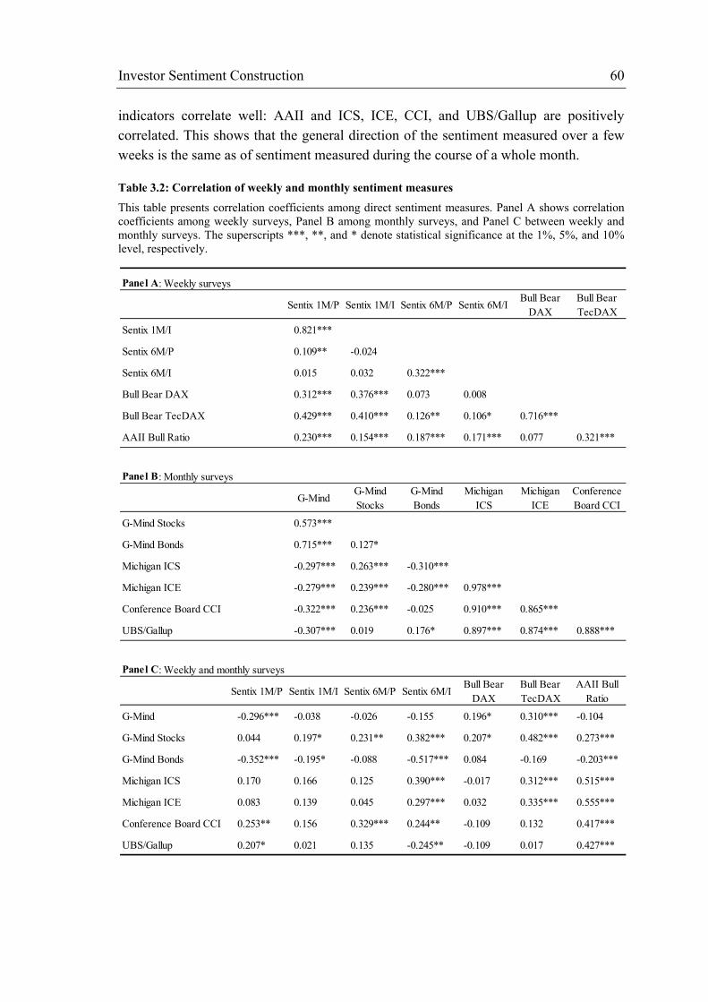
Investor Sentiment Construction 60
indicators correlate well: AAII and ICS, ICE, CCI, and UBS/Gallup are positively correlated. This shows that the general direction of the sentiment measured over a few weeks is the same as of sentiment measured during the course of a whole month.
Table 3.2: Correlation of weekly and monthly sentiment measures
This table presents correlation coefficients among direct sentiment measures. Panel A shows correlation coefficients among weekly surveys, Panel B among monthly surveys, and Panel C between weekly and monthly surveys. The superscripts ***, **, and * denote statistical significance at the 1%, 5%, and 10% level, respectively.
Panel A: Weekly surveys
Sentix 1M/P Sentix 1M/I Sentix 6M/P Sentix 6M/IBull Bear
DAXBull Bear TecDAX
Sentix 1M/I 0.821***
Sentix 6M/P 0.109** -0.024
Sentix 6M/I 0.015 0.032 0.322***
Bull Bear DAX 0.312*** 0.376*** 0.073 0.008
Bull Bear TecDAX 0.429*** 0.410*** 0.126** 0.106* 0.716***
AAII Bull Ratio 0.230*** 0.154*** 0.187*** 0.171*** 0.077 0.321***
Panel B: Monthly surveys
G-MindG-Mind Stocks
G-Mind Bonds
Michigan ICS
Michigan ICE
Conference Board CCI
G-Mind Stocks 0.573***
G-Mind Bonds 0.715*** 0.127*
Michigan ICS -0.297*** 0.263*** -0.310***
Michigan ICE -0.279*** 0.239*** -0.280*** 0.978***
Conference Board CCI -0.322*** 0.236*** -0.025 0.910*** 0.865***
UBS/Gallup -0.307*** 0.019 0.176* 0.897*** 0.874*** 0.888***
Panel C: Weekly and monthly surveys
Sentix 1M/P Sentix 1M/I Sentix 6M/P Sentix 6M/IBull Bear
DAXBull Bear TecDAX
AAII Bull Ratio
G-Mind -0.296*** -0.038 -0.026 -0.155 0.196* 0.310*** -0.104
G-Mind Stocks 0.044 0.197* 0.231** 0.382*** 0.207* 0.482*** 0.273***
G-Mind Bonds -0.352*** -0.195* -0.088 -0.517*** 0.084 -0.169 -0.203***
Michigan ICS 0.170 0.166 0.125 0.390*** -0.017 0.312*** 0.515***
Michigan ICE 0.083 0.139 0.045 0.297*** 0.032 0.335*** 0.555***
Conference Board CCI 0.253** 0.156 0.329*** 0.244** -0.109 0.132 0.417***
UBS/Gallup 0.207* 0.021 0.135 -0.245** -0.109 0.017 0.427***

Investor Sentiment Construction 61
3.4.2. Indirect Sentiment Measures
Table 3.3 shows the correlation coefficients among daily indirect sentiment measures. For the volatility indicators, first differences (denoted by Δ) are calculated in order to detect any correlation between changes of volatility (rather than levels) and other sentiment indicators.
Volatility changes (Δ VDAX as well as Δ VIX) are negatively correlated to the advance-decline measures. In addition, there are especially high positive correlations between the VDAX/VIX and the equity Put/Call ratio indicating that high volatility is usually related to increased put volume. Furthermore, the equity Put/Call ratio is negatively correlated to the ISEE Equity measure due to its similar construction methodology (the ISEE is a modified Call/Put ratio, i.e. the sign differs).
Interestingly, the TRIN measures do not have much in common: TRIN NYSE and TRIN NASDAQ are uncorrelated, and while the TRIN NASDAQ correlates well with other indicators, the TRIN NYSE does not seem to relate to any other measure. However, the TRIN NASDAQ seems to be a contrary indicator since it is positively correlated to the equity Put/Call ratio and negatively correlated to the ISEE equity measure.

Investor Sentiment Construction 62
AD
V-
DEC
DA
XA
DV
-D
EC D
JIA
Put/C
all
Tota
lPu
t/Cal
l Eq
uity
Put/C
all
Inde
xTR
IN
NY
SETR
IN
NA
SDA
QV
DA
X
Δ V
DA
XV
IX
Δ V
IXIS
EE A
llIS
EE
Equi
ty
AD
V-D
EC D
JIA
0.15
8***
Put/C
all T
otal
-0.3
71**
*-0
.113
***
Put/C
all E
quity
-0.3
35**
*-0
.129
***
0.74
0***
Put/C
all I
ndex
-0.2
08**
*-0
.125
***
0.54
1***
0.05
9**
TRIN
NY
SE0.
044
-0.0
350.
001
0.01
4-0
.034
TRIN
NA
SDA
Q-0
.276
***
-0.1
11**
*0.
282*
**0.
324*
**0.
088*
**-0
.015
VD
AX
-0
.107
***
-0.0
460.
031*
0.42
5***
-0.1
79**
*0.
114*
**0.
204*
**
Δ V
DA
X-0
.548
***
-0.1
62**
*0.
215*
**0.
265*
**0.
182*
**-0
.044
0.20
1***
0.07
3***
VIX
-0
.113
***
-0.0
65**
0.03
8**
0.44
8***
-0.1
79**
*0.
099*
**0.
268*
**0.
868*
**0.
077*
**
Δ V
IX-0
.318
***
-0.0
87**
*0.
207*
**0.
222*
**0.
186*
**-0
.210
***
0.49
6***
0.00
60.
450*
**0.
095*
**
ISEE
All
0.04
6-0
.023
-0.3
71**
*-0
.440
***
0.01
2-0
.039
-0.0
80**
*-0
.314
***
0.03
7-0
.363
***
0.00
9
ISEE
Equ
ity0.
150*
**0.
098*
**-0
.436
***
-0.6
50**
*0.
128*
**-0
.041
-0.2
42**
*-0
.458
***
-0.0
86**
-0.4
81**
*-0
.068
*0.
773*
**
ISEE
Inde
x-0
.049
-0.0
66*
0.03
60.
234*
**-0
.236
***
-0.0
040.
162*
**0.
387*
**0.
006
0.41
8***
0.01
50.
246*
**-0
.282
***
Tab
le 3
.3: C
orre
latio
n of
dai
ly in
dire
ct se
ntim
ent m
easu
res
This
tabl
e pr
esen
ts c
orre
latio
n co
effic
ient
s am
ong
daily
indi
rect
sen
timen
t mea
sure
s. Fi
rst d
iffer
ence
s ar
e de
note
d by
Δ.
The
supe
rscr
ipts
***
, **,
and
* d
enot
e st
atis
tical
sign
ifica
nce
at th
e 1%
, 5%
, and
10%
leve
l, re
spec
tivel
y.

Investor Sentiment Construction 63
3.4.3. Direct vs. Indirect Sentiment Measures
Table 3.4 and Table 3.5 show correlations between direct measures on the one hand and indirect sentiment measures on the other hand. A strong correlation implies that indirect sentiment measures contain the expectations of market participants as measured by direct sentiment.
Brown and Cliff (2004) compare direct and indirect sentiment measures and document strong relations between many disparate measures of investor sentiment. They use direct sentiment measures such as the AAII and the II surveys, and indirect measures such as the ARMS index, odd lot sales, put/call ratio, and the CEFD. They find that many commonly cited indirect measures of sentiment are related to direct measures (surveys) of investor sentiment.
Qiu and Welch (2006) investigate the CEFD measure, the Consumer Confidence survey, and the UBS/Gallup survey and validate them against each other. They compare an indirect sentiment measure with a direct measure, as well as two direct measures of consumer confidence and investor sentiment, respectively. They find that the CEFD has no correlation with the UBS/Gallup survey, while the consumer confidence index does. Regardless of the specific correlation results, it seems plausible to compare different kind of sentiment measures and the correlations among and between them.
Table 3.4: Correlation between indirect and direct weekly sentiment measures
This table presents correlation coefficients between indirect (vertical axis) and direct (horizontal axis) weekly sentiment measures. Indirect measures have been converted from daily to weekly frequency using daily averages. The superscripts ***, **, and * denote statistical significance at the 1%, 5%, and 10% level, respectively.
Sentix 1M/P Sentix 1M/I Sentix 6M/P Sentix 6M/IBull Bear
DAXBull Bear TecDAX
AAII Bull Ratio
ADV-DEC DAX 0.682*** 0.629*** 0.047 0.073 0.247*** 0.387*** 0.164***
ADV-DEC DJIA 0.105 0.107 -0.039 0.044 0.052 0.064 -0.056
TRIN NYSE -0.035 0.006 -0.024 -0.077 -0.003 -0.017 -0.017
TRIN NASDAQ -0.432*** -0.327*** -0.129** -0.161*** -0.093 -0.213*** -0.251***
VDAX -0.323*** -0.053 -0.385*** -0.058 0.112** -0.119** -0.226***
Δ VDAX -0.232*** -0.191*** -0.020 0.001 -0.106* -0.239*** -0.230***
VIX -0.302*** -0.108** -0.297*** -0.290*** 0.075 -0.156*** -0.336***
Δ VIX -0.285*** -0.239*** -0.002 0.035 -0.099* -0.244*** -0.228***
Put/Call Total -0.316*** -0.350*** -0.029 -0.012 -0.209*** -0.422*** -0.502***
Put/Call Equity -0.619*** -0.482*** -0.213*** -0.300*** -0.110* -0.318*** -0.510***
Put/Call Index -0.135** -0.130** 0.181*** 0.290*** -0.196*** -0.135** 0.025
ISEE All 0.263*** 0.145*** 0.100* 0.196*** 0.002 0.286*** 0.637***
ISEE Equity 0.519*** 0.368*** 0.145* 0.441*** -0.087 0.155* 0.537***
ISEE Index -0.180** -0.022 -0.341*** -0.487*** 0.148* -0.025 -0.326***

Investor Sentiment Construction 64
Table 3.4 presents correlations between indirect and direct weekly sentiment measures. The indirect measures (with the exception of the ADV-DEC DAX measure) are transformed to the weekly frequency using daily averages. The ADV-DEC DAX measure is an exact measure of the advances and declines per week.
There is ample of evidence that weekly survey measures are related to sentiment measures based on market data: The German private investor survey Sentix (short-term) is positively correlated to the DAX Advance-Decline measure, negatively to the equity put/call ratio and the VDAX, and positively to the ISEE Equity Index. All correlations have the direction as expected in advance: high ADV-DEC measures and high ISEE values mean positive investor sentiment whereas high put/call ratios and high VDAX levels stand for negative sentiment. Therefore, since the Sentix measure is expected to express positive sentiment, correlation coefficients differ by sign but indicate the same relationship. The institutional version of the Sentix (short-term) – due to the high correlation of 82.3% – has similar properties as the private investor version.
The AAII survey and the ISEE Index are positively correlated whereas the correlation with the put/call ratio is negative. Instead of the VDAX, the AAII measure is compared to the VIX, the U.S. volatility measure. The correlation between the AAII and the VIX is negative. The different sentiment measures express sentiment levels as expected.
The monthly direct and indirect sentiment measures are presented in Table 3.5. As for the weekly transformation, daily indirect sentiment measures have been transformed to a monthly frequency by calculating the daily averages (with the exception of the ADV-DEC DAX measure which is computed exactly as well as the CEFD for which monthly data is available).
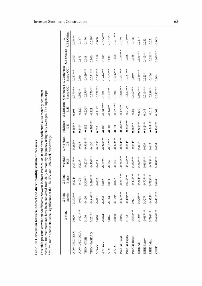
Investor Sentiment Construction 65
G-M
ind
G-M
ind
Stoc
ksG
-Min
d B
onds
Mic
higa
n IC
SΔ
Mic
higa
n IC
SM
ichi
gan
ICE
Δ M
ichi
gan
ICE
Con
fere
nce
Boa
rd C
CIΔ
Con
fere
nce
Boa
rd C
CI
UB
S/G
allu
pΔ
U
BS/
Gal
lup
AD
V-D
EC D
AX
0.02
90.
333*
**-0
.224
*0.
337*
**0.
255*
*0.
268*
*0.
195
0.37
3***
0.33
7***
0.01
00.
364*
*
AD
V-D
EC D
JIA
-0.4
21**
*-0
.091
-0.1
280.
278*
-0.0
550.
249*
-0.1
200.
362*
*0.
024
0.17
5-0
.147
TRIN
NY
SE0.
176
-0.1
500.
309*
*-0
.271
**-0
.316
***
-0.1
82-0
.236
*-0
.350
***
-0.4
29**
*0.
018
-0.1
76
TRIN
NA
SDA
Q0.
251*
*-0
.346
***
0.58
0***
-0.5
00**
*-0
.150
-0.3
92**
*-0
.121
-0.5
70**
*-0
.371
***
0.10
0-0
.249
*
VD
AX
0.07
0-0
.011
-0.0
62-0
.055
-0.1
29*
0.03
2-0
.119
*-0
.271
***
-0.2
42**
*-0
.119
-0.0
60
Δ V
DA
X-0
.044
-0.0
900.
012
-0.1
22*
-0.3
48**
*-0
.100
-0.3
00**
*-0
.071
-0.4
46**
*-0
.097
-0.3
54**
*
VIX
0.01
6-0
.114
0.00
3-0
.106
-0.1
72**
-0.0
02-0
.164
**-0
.217
**-0
.305
***
0.13
0-0
.163
*
Δ V
IX-0
.080
-0.1
29*
-0.0
22-0
.105
-0.3
23**
*-0
.074
-0.2
70**
*-0
.090
-0.4
06**
*-0
.058
-0.4
01**
*
Put/C
all T
otal
-0.0
56-0
.327
***
-0.2
11**
*-0
.761
***
-0.2
04**
*-0
.789
***
-0.1
79**
-0.6
88**
*-0
.227
***
-0.7
29**
*-0
.139
Put/C
all E
quity
0.13
2-0
.460
***
0.60
3***
-0.6
25**
*-0
.244
*-0
.542
***
-0.2
17*
-0.6
37**
*-0
.351
***
-0.2
08-0
.349
**
Put/C
all I
ndex
-0.5
38**
*0.
071
-0.4
75**
*0.
385*
**-0
.244
*0.
268*
*-0
.184
0.63
2***
-0.0
39-0
.158
-0.1
78
ISEE
All
0.18
6*0.
526*
**-0
.554
***
0.56
5***
0.21
1*0.
551*
**0.
159
0.30
2***
0.31
9***
0.33
1***
0.21
1*
ISEE
Equ
ity-0
.617
***
0.32
7*-0
.707
***
0.69
8***
0.07
90.
642*
**0.
045
0.71
9***
0.32
3*0.
413*
*0.
243
ISEE
Inde
x0.
716*
**-0
.335
**0.
713*
**-0
.788
***
0.04
7-0
.743
***
-0.0
15-0
.839
***
-0.1
66-0
.511
**-0
.271
CEF
D
-0.6
40**
*-0
.451
***
0.04
40.
519*
**0.
054
0.43
6***
0.06
30.
655*
**0.
064
0.66
0***
-0.0
05
Tab
le 3
.5: C
orre
latio
n be
twee
n in
dire
ct a
nd d
irec
t mon
thly
sent
imen
t mea
sure
s
This
tabl
e pr
esen
ts c
orre
latio
n co
effic
ient
s bet
wee
n in
dire
ct (v
ertic
al a
xis)
and
dire
ct (h
oriz
onta
l axi
s) m
onth
ly s
entim
ent
mea
sure
s. In
dire
ct m
easu
res h
ave
been
con
verte
d fr
om d
aily
to m
onth
ly fr
eque
ncy
usin
g da
ily a
vera
ges.
The
supe
rscr
ipts
**
*, *
*, a
nd *
den
ote
stat
istic
al si
gnifi
canc
e at
the
1%, 5
%, a
nd 1
0% le
vel,
resp
ectiv
ely.

Investor Sentiment Construction 66
The monthly G-Mind Stocks measure is negatively correlated to the equity put/call ratio and positively to the ISEE equity index as well as the DAX ADV-DEC measure. Interestingly, the G-Mind Bonds is also correlated but in the opposite direction: There is a positive correlation to the equity put/call ratio and a negative correlation to the ISEE equity index. The reason is the opposite expectation of investors towards the asset classes stocks and bonds: When investor sentiment towards stocks is rather negative, investors tend to buy bonds, and vice versa. Therefore, correlation coefficients have different signs.
The monthly U.S. confidence and sentiment surveys have a lot in common: They all correlate well with the CEFD and the total put/call ratio, though the direction differs: Correlation with CEFD is large and positive indicating that all measure a common source of sentiment. However, correlation with the total put/call ratio is large and negative which confirms that the put/call ratio typically is a contrary indicator. With the exception of the CCI, all other surveys are also positively correlated to the ISEE total index.
The results presented in this section confirm Qiu and Welch’s (2006) finding that the UBS/Gallup measure and the Michigan ICS are positively correlated (89.7%) and that they are indeed likely to pick up the same underlying factor – investor sentiment. In contrast to their original study, however, the results of this section show that the UBS/Gallup measure and the CEFD as reported by Baker and Wurgler (2006)17 are also positively correlated: A large and highly significant 66% correlation suggests that the CEFD may also pick up the same investor sentiment.
3.4.4. Sentiment Measures vs. Market Returns
Brown and Cliff (2004) investigate the correlation of sentiment and market returns and find that changes in the survey and their composite measures of investor sentiment are highly correlated with contemporaneous market returns.
The contemporaneous correlations between all sentiment indices and market returns are presented in Table 3.6. Panel A shows correlations between market returns and daily sentiment measures, Panel B weekly sentiment measures, and Panel C monthly sentiment measures.
17 Jeffrey Wurgler makes the CEFD data available on his website (http://pages.stern.nyu.edu/~jwurgler/). They take the value-weighted average discount on closed-end stock funds for 1962 through 1993 from Neal and Wheatley (1998), for 1994 through 1998 from CDA/Wiesenberger, and for 1999 through 2001 from turn-of-the-year issues of the Wall Street Journal.

Investor Sentiment Construction 67
Table 3.6: Correlation of sentiment measures and market returns
This table presents correlation coefficients between sentiment measures and market logreturns as proxied by several international stock market indexes. Panel A presents coefficients for daily, Panel B for weekly, and Panel C for monthly sentiment measures. The superscripts ***, **, and * denote statistical significance at the 1%, 5%, and 10% level, respectively.
As a proxy for market returns, we use several indices: the DAX for the German market, the EuroStoxx50 for the European market, the S&P500, the NASDAQ100, and the
DAX TecDAX ESX50 S&P 500 Nasdaq 100 DJIA Russel 2000 REX
ADV-DEC DAX 0.785*** 0.673*** 0.760*** 0.369*** 0.355*** 0.370*** 0.368*** -0.153***
ADV-DEC DJIA 0.132*** 0.142*** 0.147*** 0.120*** 0.116*** 0.124*** 0.101*** -0.022
Put/Call Total -0.264*** -0.257*** -0.272*** -0.257*** -0.228*** -0.240*** -0.276*** 0.097***
Put/Call Equity -0.372*** -0.361*** -0.354*** -0.290*** -0.283*** -0.279*** -0.297*** 0.113***
Put/Call Index -0.185*** -0.163*** -0.194*** -0.195*** -0.197*** -0.194*** -0.219*** 0.024
TRIN NYSE 0.206*** 0.183*** 0.200*** 0.209*** 0.195*** 0.217*** 0.131*** -0.200***
TRIN NASDAQ -0.372*** -0.349*** -0.344*** -0.634*** -0.746*** -0.604*** -0.608*** 0.081***
VDAX -0.099*** -0.076*** -0.086*** -0.041*** -0.014 -0.040** -0.053*** 0.053***
Δ VDAX -0.649*** -0.577*** -0.712*** -0.346*** -0.258*** -0.334*** -0.341*** 0.120***
VIX -0.120*** -0.127*** -0.117*** -0.128*** -0.074*** -0.120*** -0.139*** 0.064***
Δ VIX -0.437*** -0.416*** -0.486*** -0.784*** -0.548*** -0.751*** -0.693*** 0.137***
ISEE All -0.026 0.006 -0.043* -0.012 -0.045* -0.016 0.007 0.007
ISEE Equity 0.153*** 0.173*** 0.131*** 0.114*** 0.130*** 0.108*** 0.109*** -0.077**
ISEE Index -0.086** -0.084** -0.092** -0.068* -0.090** -0.067* -0.053 0.049
Sentix 1M/P 0.542*** 0.500*** 0.512*** 0.469*** 0.485*** 0.451*** 0.461*** -0.283***
Sentix 1M/I 0.490*** 0.446*** 0.474*** 0.411*** 0.432*** 0.406*** 0.413*** -0.233***
Sentix 6M/P 0.042 0.070 0.047 0.019 0.049 0.011 0.036 -0.078
Sentix 6M/I -0.002 0.066 0.029 0.038 0.089* 0.010 0.043 -0.051
Bull Bear DAX 0.174*** 0.128** 0.180*** 0.168*** 0.189*** 0.172*** 0.179*** -0.034
Bull Bear TecDAX 0.328*** 0.321*** 0.319*** 0.268*** 0.266*** 0.245*** 0.271*** -0.070
AAII Bull Ratio 0.193*** 0.188*** 0.170*** 0.148*** 0.103** 0.137*** 0.183*** -0.138***
Δ G-Mind 0.082 -0.041 0.078 0.045 0.022 0.071 -0.023 0.235**
Δ G-Mind Stocks 0.068 -0.024 0.088 0.043 0.030 0.072 -0.005 -0.014
Δ G-Mind Bonds 0.000 -0.040 -0.029 -0.069 -0.006 -0.083 -0.114 0.360***
Δ Michigan ICS 0.209*** 0.172* 0.211** 0.165** 0.052 0.166** 0.230*** -0.121
Δ Michigan ICE 0.176** 0.161* 0.185** 0.126* 0.040 0.127* 0.191*** -0.107
Δ Conference Board CCI 0.297*** 0.143 0.292*** 0.245*** 0.117 0.252*** 0.302*** -0.227**
Δ UBS/Gallup 0.316*** 0.254** 0.281*** 0.245** 0.245** 0.200** 0.345*** -0.216**
Logreturns
Panel A: Daily sentiment measures
Panel B: Weeky sentiment measures
Panel C: Monthly sentiment measures

Investor Sentiment Construction 68
broader Russell 2000 for the American market. Also, we have included the REX index, the German Index for government bonds, to detect correlations between this index and the German G-Mind Bonds measure.
The following findings can be noted for the daily measures: The advance/decline measure for the DAX is positively correlated to contemporaneous DAX returns which is not surprising since DAX returns are positive when there are more advancing stocks than declining. The relationship is not linear, however, due to the different weights of the member stocks. The equity put/call ratio and equity market returns are negatively correlated. This means that market rises are accompanied by large call volumes and market declines by large put volumes. In other words, the put/call ratio measured at the CBOE moves with the market and supports market movements.
High negative correlations exist between the TRIN NASDAQ measure and contemporaneous market returns, especially of the NASDAQ 100. One usually sees high TRIN readings near market lows and extended periods of low readings near market peaks. This means that the TRIN can be used as a contrary indicator.
Changes of the VIX are negatively correlated to S&P 500 returns and other American market index returns. This finding is in line with related research about volatility and returns (e.g. Whaley 2000). If expected market volatility increases, investors demand higher rates on returns on stocks, and so stock prices fall. The same relationship applies to the German volatility measure, the VDAX, and the DAX returns.
The ISEE Sentiment, although its construction suggests that its behavior is contrary to that of the put/call ratios, does not correlate to such a large extent with market returns. Correlation of the ISEE equity index and market returns is significantly positive but economically small.
The weekly short-term surveys show a positive correlation with market returns, especially the DAX. The Sentix private investor survey’s correlation amounts to 54.2% and the Sentix institutional investor survey’s correlation to 49.0%. The medium-term surveys, however, do not correlate with contemporaneous market returns. The Bull Bear ratios and the AAII survey are significantly positively correlated to market returns, though correlation is not very high.
Changes in the monthly surveys show a medium positive correlation with market returns, especially the DAX. Survey levels do not exhibit any correlation (and are therefore not presented in Table 3.6). Correlation coefficients of the G-Mind are low and not significant with the exception of the G-Mind Bonds Index and the REX. They correlate significantly with a correlation coefficient of 36.0%.

Investor Sentiment Construction 69
3.4.5. Review of Results
The purpose of section 3.3.4 was to investigate three main questions: First, do direct or indirect investor sentiment measures pick up the same signals and therefore correlate within each group? Second, are direct and indirect measures correlated and can they be validated against each other? Third, are investor sentiment measures correlated to market returns and therefore explain part of the movements of the market?
Firstly, an overall high correlation among survey measures can be documented although they generally have a different set of respondents (e.g. Sentix and Bull Bear TecDAX have a 40% correlation). Furthermore, correlations among surveys conducted in different countries are correlated (e.g. Sentix in Germany and AAII in the U.S. have a 23.0% correlation) with the exception of the G-Mind. Although survey frequencies may be different (e.g. the weekly AAII survey and the monthly G-Mind survey), high correlations of up to 51.7% are documented.
Secondly, most direct and indirect measures can be successfully validated against each other: Correlations between weekly and monthly surveys on the one hand and indirect measures on the other hand are generally very high and have the expected direction. The high-to-low frequency conversion, however, could possibly disguise a higher correlation at the monthly levels.
Thirdly, the majority of all sentiment indicators (or their first differences) is correlated to market returns, higher correlations for high-frequency measures and lower correlations for lower-frequency measures are documented. The direction of the correlation, however, is not unanimous: Most survey measures have a positive correlation with stock market returns whereas the results for the indirect daily measures are mixed. Especially changes in the VDAX/VIX and the NASDAQ Traders Index (TRIN) are negatively correlated with market returns.
3.5. Conclusion In this chapter, different classifications of investor sentiment measures are presented as suggested by related research and sentiment measures in practice. Direct sentiment measures are surveys in which investors are asked directly about their attitude towards the economic situation or the stock market in particular. Indirect sentiment measures refer to financial variables and require a theory relating them to sentiment. Meta-measures are sentiment measures that are neither based on surveys nor pure financial data but involve meta-information about investor sentiment.
In research, the closed-end funds discount has received a great deal of attention in the 1990s. Today, researchers still cannot explain the existence of a CEFD and its variance. Many other studies have tried and are still trying to create composite or meta-measures

Investor Sentiment Construction 70
to extract investor sentiment that is useful for explaining investor behavior and/or market returns.
In practice, there are many investor sentiment measures whose usefulness is widely debated in the media. Many of the measures involve the polling of investors, the collection of financial data and the construction of technical indicators.
The evaluation of sentiment measures is difficult and not straightforward. Qiu and Welch (2006) state that “we have what we believe to be the best available empirical direct proxy for investor sentiment” and measure the quality of a sentiment index according to its correlation with their direct measure of sentiment. In general, most of the measures, regardless of whether they are indirect or direct, have a high pairwise correlation indicating that they indeed pick up the same sentiment signal. Therefore, correlation with other sentiment measures could serve as an indicator for sentiment quality, but not as a necessary or sufficient condition.
Another evaluation method of sentiment measures is the comparison with market returns. Since investor sentiment incorporates investors’ expectations and opinion about the market, sentiment measures and market returns should be correlated. We confirm this reasoning and find that most of the sentiment indicators correlate well with market returns, with high-frequency indirect measures having the highest correlation and lower-frequency indirect measures a lower correlation with the market.
To sum up, there are many different measures of investor sentiment in research and practice but their evaluation remains difficult. A high correlation among each other and with market returns is a good indication that they react to the same underlying factor. Future research, however, is needed to identify this factor which will make it easier to construct new measures and evaluate existing ones.

Construction of the Euwax Sentiment Index 71
4 Construction of the Euwax Sentiment Index
Using a unique data set consisting of more than 36.5 million submitted retail investor orders over the course of 5 years, the Euwax Sentiment Index is being developed. It is based on retail investor orders submitted to the European Warrant Exchange, the market segment for securitized derivatives at Boerse Stuttgart. What makes this data unique is the fact that it consists of retail orders only, retail buy and sell orders can be determined exactly due to the market maker model, expression of negative sentiment is possible by buying puts, and not the data includes executed as well as submitted orders.
This chapter is structured as follows: Section 4.1 presents an introduction of structured products in general and trading at EUWAX in particular and summarizes key facts. The data set is described in 4.2. The basic index calculation is shown in section 4.3, followed by multivariate regressions that determine the influence of certain parameters on the index in section 4.4. Finally, section 4.5 compares the Euwax Sentiment Index with other direct and indirect sentiment measures found in practice. Section 4.6 concludes this chapter.
4.1. Introduction
4.1.1. Securitized Derivatives
History of securitized derivatives
The history of securitized derivatives started in the 1980s with the creation of covered warrant markets in Switzerland and Germany (a detailed history of covered warrants can be found in McHattie 2002). Since then, covered warrants have been established in many European countries, among them France, Italy, and the United Kingdom. Covered warrants are securities issued by banks or financial institutions representing the right for the investor to buy or sell an asset at a fixed price, on or before a specified future date.
In particular, covered warrants may give rights over single stocks, a basket of stocks, an index, a currency, a commodity, or any other financial asset. Investors thereby gain exposure to the performance of an asset for a fraction of a price. This is called gearing. The name ‘covered’ warrant was coined when these financial products held the right to purchase a physical stock at the end of their term. The issuer of the warrant commonly held the stock in order to be able to satisfy the right when the warrant reached maturity.

Construction of the Euwax Sentiment Index 72
Therefore, the warrant was covered by the underlying security. Today, issuers use dynamic hedging techniques to cover their financial exposure.
Today, covered warrants make up only a fraction of all traded securitized derivatives. Issuers have continually advanced their products to meet growing investors’ demands. Knock-out certificates (also known as mini-futures) have been invented as well as investment certificates. In general, a distinction between leverage products (i.e. products with a gearing) and investment products (i.e. usually 100% participation with no gearing) can be made.
Types and terms
The term “warrant” is very broad and stands for a highly flexible instrument which can be transformed to match a wide range of demands. However, there are several types and terms all these instruments have in common.
Calls and puts: With securitized derivatives, investors can benefit from both rising and falling markets by choosing call products or put products. Like in the traditional options market, call products give a right to buy an underlying asset whereas put products entitle the holder to sell the underlying asset at a predetermined price. Most investors are by nature optimistic, and a falling market is usually an opportunity for them to find the bottom. However, in recent years investors have gained more and more experience with the opportunity to speculate on falling markets, so that put products have become popular instruments for retail investors.
Exercise style: The exercise terms of plain-vanilla warrants are usually described by the terms ‘European style’ and ‘American style’. European exercise style means that the warrants can only be exercised on a specific date whereas American exercise style means that they can be exercised at any point in time to maturity. Exercising a warrant means that investors make use of their right to buy or sell the underlying asset at the predetermined price. Therefore, issuers prefer the European style because exercise occurs infrequently, and investors may prefer the American style since it offers more flexibility. In practice, however, this difference does not matter much since most investors never exercise their warrants and rather sell them before maturity.
Strike prices: For leverage products, the strike price is the primary determinant of leverage and associated risk. The strike price is the specified price at which the warrant may be exercised, i.e. the price at which call option buyers can buy the underlying and at which put option buyers can sell the underlying. In practice, the ratio of the strike price to the underlying spot price determines the risk of the product. The difference of the strike and the spot price is the intrinsic value of the warrant.

Construction of the Euwax Sentiment Index 73
Pricing and trading
Prices of securitized derivatives are not driven by supply and demand like in traditional order-driven markets for equities and traditional listed warrants. The issuer is usually the sole market-maker who is obliged to make a two-way price throughout the trading day. Quotes are commonly derived from underlying prices in their respective liquid order-driven markets. Computers automatically calculate quotes and distribute them to exchanges, order flow providers, and financial web portals.
A single-market-maker-model is common in the established markets for securitized derivatives. However, competition is far from absent: Competition simply occurs across products rather than within a particular security. On popular underlyings, several issuers offer products with similar terms, i.e. similar strike prices and maturity. In addition, issuer reputation plays an important role in competition: If an issuer makes prices to the detriment for the investor, such as widening the spread during times of financial stress, investors will quickly become aware of that and the issuer will lose business. These two forces – inter-product competition and reputation – usually ensure a fair and orderly market.
Fair prices are calculated taking a number of different factors and assumptions into account which may vary from issuer to issuer. These factors are the underlying asset price, the volatility of the underlying, the time to expiry, dividend yields, and the interest rate of a risk-free asset. Basically, the well-known options pricing model of Black and Scholes (1973) is based on these factors, but issuers may arrive at different prices due to different assumptions about volatility or interest rate development. However, the inter-product competition leads to a general convergence of market-maker quotes for popular underlyings.
Advantages
There are many advantages for retail investors when investing in securitized derivatives. Securitized derivatives, especially warrants and knock-outs, provide retail investors with gearing and leverage. Gearing is defined as the degree of additional exposure gained by buying a warrant. It is calculated by dividing the asset price by the warrant price. Leverage measures how much more a warrant will move in percentage terms against the underlying asset. It is calculated by multiplying the gearing with the delta which represents the change expected in the price of a warrant for a given change in the underlying instrument.
Gearing is an obvious advantage for investors because it is a way to achieve a large equity exposure from a relatively small amount of money. Sometimes, gearing-up and gearing-down are differentiated but the concept is essentially the same. Gearing-up means that e.g. a warrant investment of 5.000€ can lead to a much higher exposure of

Construction of the Euwax Sentiment Index 74
25.000€. Gearing-down means the investor’s aim is to gain an equity exposure of 5.000€ and therefore invest only 1.000€ in warrants.
Another advantage of warrants for investors is the fact that warrants (and other securitized derivatives) are securities as opposed to contracts in futures and options markets. Securities have the property that their value can never be smaller than zero, so that investors’ losses are limited by their initial investment. In futures markets, investors face the possibility to lose more than their initial investment. Therefore, warrant investors have the chance to unlimited gains while their losses are limited.
In contrast to equity markets, retail investors have opportunities in both Bull and Bear markets. While short-selling of stocks is usually not possible for retail investors, put warrants and other short products provide the opportunity to speculate on falling markets.
Securitized derivatives in general also provide the retail investor with the ability to invest in assets otherwise unavailable to them. For example, they can be based on currencies, baskets of stocks or commodities, foreign indices or stocks which are not traded in their home market. In addition, in most of the cases, securitized derivatives are a low transaction cost alternative to investing in the underlying stocks directly.
Disadvantages
Credit Risk must be mentioned as one of the disadvantages of securitized derivatives, especially since the financial market crisis when the investment bank and issuer Lehman Brothers went into bankruptcy and many retail investors suffered losses because they held investment certificates issued by this bank. However, credit risk has received a lot of attention lately, and the majority of retail investors now know the possible dangers linked to issuer default risk. Transparency has been increased and credit risk has become an integral part of the decision process of retail investors.
Complexity can be mentioned as another disadvantage when considering securitized derivatives. One driver is the higher complexity of derivative products in contrast to stocks – prices are derived and their calculation can be complex because many factors such as interest rates, volatility, etc. determine prices. Another driver is the amount of products available to retail investors: More than 380.000 products securitized derivatives were listed at the end of October 2009 in the EUWAX segment at Boerse Stuttgart. However, the large amount of products is due to different issuers, different strike prices, and different underlyings. If retail investors know their preferred issuer, underlying, and strike price (i.e. risk) in advance, there are several finders on the internet that help retail investors find the product that fits their needs best.
Usually, securitized derivatives do not rank for any income, i.e. they do not qualify for dividend payments on underlyings because these payments are usually used by the

Construction of the Euwax Sentiment Index 75
issuer to finance the specific structure. There are exceptions like DAX certificates that incorporate dividends because the DAX is a so-called performance-index that includes dividend payments of the stock index members. In addition, and common to all securitized derivatives, holders have no voting rights and do not receive annual or interim reports as they are not directly linked to that company. Usually, this disadvantage is not important for retail investors because most of them usually do not make use of their voting rights.
4.1.2. European Warrant Exchange
EUWAX is the trading segment for securitized derivatives at Boerse Stuttgart. It is Europe’s largest trading platform for securitized derivatives in terms of turnover and number of trades. Securitized derivatives comprise a wide range of securities, e.g. covered warrants (bank-issued options), knock-out certificates (bank-issued barrier options), and investment certificates. They all have in common that their value depends on another financial instrument such as stocks, indices, commodities or fixed income products. Securitized derivatives are usually issued by banks which are obliged to continuously calculate and publish bid and ask prices for their products.
Executed order volume in securitized derivatives accounts for about 3.5 billion Euros per month totaling 211.7 billion Euros for the period of January 2004 to December 2008). At the end of the sample period, more than 150,000 leverage products and more than 180,000 investment products were listed. As a retail investor exchange, Boerse Stuttgart tailors its products and services offered to retail investors. The design of the issued securities is such that they are largely unattractive to institutional investors, but all the more appealing to retail investors. Products are not standardized and strike prices, duration, underlyings, payoff profile, and multiplier all vary from product to product. They are constructed in order to attract retail investors that value variability, dynamic combinations of underlyings, and optically low prices. These characteristics actively dissuade institutional investors that typically value standard and therefore easily hedged products, low counterparty risk, liquidity, and volume. These market characteristics and general acceptance that large investors avoid these types of markets obviate the need to control for institutional investors’ influence in the data set.
4.1.3. Key Facts
Quote-driven market
Trading at the EUWAX takes place in a quote-driven market where market-makers continuously publish quotes. There are two kinds of trading participants in this context: Firstly, there are the market-makers (usually the product issuers) who publish bid and ask quotes for their products. Secondly, there are order flow providers (usually banks or brokerages) who route client orders to the exchange. Thirdly, there are quality liquidity

Construction of the Euwax Sentiment Index 76
providers acting on behalf of the exchange who assist in the matching procedure by providing quality and liquidity. They also continuously check the order book for executable orders and start the matching procedure.
This type of market model allows a distinction of retail orders and market maker orders. Our main assumption is that retail investors express their expectations about the market by buying and selling derivatives whereas issuers do not express any opinion because they have an obligation to trade. A retail investor’s order can therefore be matched either against an issuer’s order which will be the usual case, or against another retail investor’s order from the order book.
Risk
The derivative products listed at EUWAX can be categorized as either leverage or investment products. Leverage products comprise covered warrants and knock-out certificates whereas investment products comprise all types of investment certificates.
Derivative products can be further categorized according to the risk inherent in their structure. Leverage products are usually regarded as riskier than investment products because investors face the risk of losing their whole investment in a relatively short time period. Knock-outs, for example, are worthless when the price of the underlying falls below (down and out) or goes above (up and out) a specific price. Investment certificates, on the other hand, usually exhibit some security features so that the investor is partially protected against a total loss.
Positive and negative sentiment
For each product category there are two basic option types: calls and puts. The purchase of a call option can be interpreted as a positive sentiment about the future return of the underlying whereas the purchase of a put option can be interpreted as a negative sentiment about the future value of the underlying. Although the terms call and put are typically used in the options market, this distinction can also be made in the securitized derivatives market.
The possibility of buying puts is a clear advantage of the data set since investors have the opportunity to express negative sentiment without the need for short sales. On most retail investor exchanges, short selling is constrained to professional investors.
4.2. Data Set The data set contains order data from the EUWAX trading segment at Boerse Stuttgart for the period of January 2004 to December 2008. This data set contains 24,348,822 executed orders from retail investors. Market maker orders are not taken into account. The whole set of orders account for a volume of about 211.7 billion Euros. Table 4.1

Construction of the Euwax Sentiment Index 77
reports summary statistics of the number of executed orders during the whole sample period. Statistics are grouped along four dimensions: product group (horizontal axis), option type (Panel A), order type (Panel B), and underlying type (Panel C).
Summary statistics of the volume of executed orders as well as the number of submitted orders are similar to these reported in Table 4.1 and can be found in Appendix A.
Table 4.1: Summary statistics
This table reports summary statistics about the number of executed orders by derivative product group (warrants, knock-outs, and investment certificates). Panel A groups the orders by option type and trade direction, Panel B by order type, and Panel C by underlying type. The percentages in brackets provide information about the relative frequency of the different order classes within each product group.
As can be expected from a retail investor exchange, call products account for more than 76% of the total number of orders whereas puts for only 24%. This is mostly due to the fact that most retail investors neither have the knowledge nor the willingness to trade put products. Due to the short-term nature of leverage products, there are more executed
Call Buy 3,553,189 (43.5%) 3,727,704 (34.1%) 2,703,625 (51.6%) 9,984,518 (41.0%)
Sell 2,791,118 (34.1%) 3,468,948 (31.7%) 2,416,436 (46.1%) 8,676,502 (35.6%)
Put Buy 1,003,689 (12.3%) 1,885,706 (17.3%) 67,266 (1.3%) 2,956,661 (12.1%)
Sell 829,584 (10.1%) 1,845,794 (16.9%) 55,763 (1.1%) 2,731,141 (11.2%)
8,177,580 10,928,152 5,243,090 24,348,822
Panel B: Executed orders by order type
4,727,776 (57.8%) 5,813,977 (53.2%) 4,172,416 (79.6%) 14,714,169 (60.4%)
2,901,586 (35.5%) 3,008,653 (27.5%) 899,047 (17.1%) 6,809,286 (28.0%)
548,218 (6.7%) 2,105,522 (19.3%) 171,627 (3.3%) 2,825,367 (11.6%)
8,177,580 10,928,152 5,243,090 24,348,822
Panel C: Executed orders by underlying type
4,537,798 (55.5%) 2,234,376 (20.4%) 2,241,935 (42.8%) 9,014,109 (37.0%)
2,739,865 (33.5%) 6,702,157 (61.3%) 2,432,471 (46.4%) 11,874,493 (48.8%)
55,212 (0.7%) 174,622 (1.6%) 80,236 (1.5%) 310,070 (1.3%)
445,337 (5.4%) 502,380 (4.6%) 8,649 (0.2%) 956,366 (3.9%)
391,975 (4.8%) 1,032,518 (9.4%) 428,691 (8.2%) 1,853,184 (7.6%)
Other 7,393 (0.1%) 282,099 (2.6%) 51,108 (1.0%) 340,600 (1.4%)
8,177,580 10,928,152 5,243,090 24,348,822Total
Indices
Fixed Income
Currencies
Commodities
Knock-outs Investment certificates Total
Total
Stocks
Knock-outs Investment certificates Total
Warrants
Warrants
Market Orders
Limit Orders
Stop Orders
Total
Panel A: Executed orders by option type
Warrants Knock-outs Investment certificates
Total

Construction of the Euwax Sentiment Index 78
put orders in leverage products (warrants and knock-outs) than in investment products. The ratio of puts in leverage products amounts to more than 29%.
Retail investors at Boerse Stuttgart have a choice of the following order types: They can submit market orders without specifying a price, limit orders with a limit price, and stop orders with a stop limit. Due to the market-maker model, market orders are always executed against the market-maker quote, so retail investors do not face the risk of being executed at an inferior price than quoted. Investors submitting limit orders may want to save the spread that they pay when submitting market orders. Stop orders are activated when the market-maker quote reaches the stop limit. An activated stop order becomes a market order and is executed immediately.
For the purposes of this study, all orders are sorted according to their order type into three groups: The first group, market orders, contains market orders as well as marketable limit orders and marketable stop orders. Orders are defined as marketable if they are submitted with a (stop) limit and executed within 60 seconds of submission. The rationale behind this classification is that market orders without a limit and limit orders with a very aggressive limit should be treated the same since investors often use them interchangeably. The second and third groups are limit orders and stop orders with a limit that prevents orders from being executed immediately. These orders should be treated separately. Panel B of Table 4.1 shows the number of executed orders by order type.
The use of the different order types differs across instruments. Market orders are used more frequently when trading investment products than leverage products. One reason for that is that investors have longer horizons and do not care about the spread they have to pay by using market orders. Stop orders are used most often when trading knock-out certificates due to their higher risk level. Overall, retail investors prefer market orders over other order types.
Panel C of Table 4.1 presents the number of executed orders and their relative distribution by underlying type of the traded products. Each derivative product’s underlying can be categorized into different underlying categories such as stocks, indices, commodities, currencies, or fixed income products. Indices and individual stocks are the most used underlyings for securitized derivatives and account for more than 85% of the number of executed orders. Among the most traded equity underlyings are Allianz, Daimler, Deutsche Bank, Deutsche Telekom, Siemens, SAP, and Munich Re. The most traded index underlyings are the DAX, EuroStoxx, and Nikkei equity indices. Commodities include Brent Crude Oil, Gold, and Silver futures. Volume in Fixed Income underlyings is highest for Euribor and Bund Futures.

Construction of the Euwax Sentiment Index 79
4.3. Basic Index Calculation Intuitively, positive investor sentiment should be expressed by a high index level, and negative investor sentiment by a low index level. The intuition of the index level is the following: Bullish investors buy calls or sell puts whereas bearish investors sell calls or buy puts. Therefore, order volume is categorized as driven by positive and negative sentiment and the ratio of the net order volume to the overall order volume is calculated.
As a requirement for the index design, the index should be invariant to a rise or drop in overall order volume, i.e. the index values should not depend on the absolute order volume but rather on the relative proportion of buy and sell order volumes. Therefore, investor sentiment values are not influenced by an overall rise in market volume.
The sentiment index is calculated for a given time period t as follows
_ ∑ · ·∑ (4.1)
_ ∑ ·∑ (4.2)
where
vi … transaction volume of order i (trade price × trade size) oi … option type of the instrument traded through order i
(oi = 1 call option, oi = -1 put option) ti … trade direction of order i (ti = 1 buy order, ti = -1 sell order)
Sentiment can be calculated using either the aggregate order volume (see formula 4.1) or the number of executed orders (see formula 4.2). Time periods used for calculation can be daily, weekly, or monthly. The higher the frequency, the noisier becomes the index. On the other hand, when choosing a lower frequency, e.g. monthly, the resulting index has less granularity and less overall descriptiveness.
Instead of choosing different calculation periods, a moving average of the daily index calculation can be introduced in order to reduce noise. A backward-looking moving average of the daily index calculation seems to be the most appropriate because noise is reduced, trends can be recognized, and a new index value is calculated every day. A disadvantage, however, is that sudden changes in the investor sentiment are not represented immediately as a delay is introduced as an artifact of the backward-looking moving average.
Before a more detailed analysis of different aspects of sentiment construction is performed, Figure 4.1 plots the 20-day moving average of the daily sentiment index based on the number of all executed orders in derivative products.

Construction of the Euwax Sentiment Index 80
Figure 4.1: Euwax Sentiment Index (2004 – 2008)
These figures (above and next page) show the 20-day moving averages of the Euwax Sentiment Index based on the number of executed orders in all derivative products (investment products and leverage products) along with the daily DAX close prices.
-.2
-.1
.0
.1
.2
.3
3,600
3,800
4,000
4,200
4,400
2004Q1 2004Q2 2004Q3 2004Q4
Euwax Sentiment DAX
Euw
ax S
entim
ent
DA
X
-.2
-.1
.0
.1
.2
.3
4,000
4,400
4,800
5,200
5,600
2005Q1 2005Q2 2005Q3 2005Q4
Euwax Sentiment DAX
Euw
ax S
entim
ent
DA
X

Construction of the Euwax Sentiment Index 81
Figure 4.1: Euwax Sentiment Index (2004 – 2008) – cont’d
-.2
-.1
.0
.1
.25,200
5,600
6,000
6,400
6,800
2006Q1 2006Q2 2006Q3 2006Q4
Euwax Sentiment DAX
DAX
Euw
ax S
entim
ent
-.15
-.10
-.05
.00
.05
.10
.15
.20
6,400
6,800
7,200
7,600
8,000
8,400
2007Q1 2007Q2 2007Q3 2007Q4
Euwax Sentiment DAX
DA
X
Euw
ax S
entim
ent
-.2
-.1
.0
.1
.2
4,000
5,000
6,000
7,000
8,000
2008Q1 2008Q2 2008Q3 2008Q4
Euwax Sentiment DAX
DAX
Euw
ax S
entim
ent

Construction of the Euwax Sentiment Index 82
4.4. Sentiment Analysis The purpose of this section is to further understand the influence of certain aspects of the raw order flow on the sentiment index construction and relate it to contemporaneous market returns. The sentiment measure and its different order flow components are compared to market returns because if sentiment is a driver of equity prices, correlations should be found between its measurement and market returns.
Multivariate regressions are used that test how different sentiment measures influence market returns and how much of the variance in the market returns can be explained by investor sentiment.
4.4.1. Number vs. Volume Based Measures
Different components of the order flow can be distinguished: buy call volume, sell call volume, buy put volume, and sell put volume. In order to be invariant from an overall rise or fall of absolute order volume, the ratio of all order flow subgroups to the sum of the order flow is calculated for each order flow component as follows:
_ _ _ __
(4.3)
_ _ _ __
(4.4)
_ _ _ __
(4.5)
_ _ _ __
(4.6)
where total_volume is the sum of buy call, sell call, buy put, and sell put volume in a certain time period. Order flow ratios are calculated for all product categories and two sub categories, namely leverage products (i.e. warrants and knock-out certificates) and investment certificates. In addition, ratios are calculated using the number of executed orders instead of the executed order volume.
A multivariate linear regression (see equation 4.7) is performed with the DAX logreturns as the dependent variable and the order flow ratios as independent variables. Newey-West standard errors are used that are robust to heteroskedasticity.
dax_logreturns = β1 buy_call_ratio + β2 sell_call_ratio (4.7) + β3 buy_put_ratio + β4 sell_put_ratio
Regression results are presented in Table 4.2 and Table 4.3. The first table shows the results for sentiment measures that are based on the volume of executed orders whereas the second table is based on the number of executed orders. For each table, results are presented for ratios based on different input parameters: Panel A presents results

Construction of the Euwax Sentiment Index 83
differentiated by product type, Panel B by option type, and Panel C by volume group. Panel D provides results for submitted orders.
The adjusted R² values indicate the amount of variance explained by the model. The adjusted R² value of 0.5626 (Table 4.3) can be interpreted in a way that 56% of the variance of the DAX logreturns can be explained by the sentiment measure based on the number of executed orders. The model that uses sentiment ratios based on the volume of executed orders (Table 4.2) receives an R² value of 0.4752 which is lower than the number based model.
The difference can be explained by possible outliers caused by extremely high volume orders that belong to a few wealthy individuals. In this case, retail investor sentiment is not based on the majority of individuals but rather the majority of the capital invested – and therefore does not represent the overall opinion of the market participants.
Taking this finding into account, further analyses focus on the number of executed or submitted orders instead of their order volume.

Construction of the Euwax Sentiment Index 84
Table 4.2: Multivariate regression results for order volume
This table presents regression results for the multivariate linear regression as presented in formula 4.7. Executed order volume is used to construct the ratios. Panel A presents results for ratios based on the volume of executed orders by product type. Panel B differentiates executed orders by order type and Panel C by order volume group. Panel D provides information about regression results using submitted order volume instead of executed order volume. The superscripts ***, **, and * denote statistical significance at the 1%, 5%, and 10% level, respectively.
adj. R²
Panel A: Executed order volume by product type
all products -0.0053 *** 0.0064 *** 0.0497 *** -0.0554 *** 0.4752
leverage products -0.0050 *** 0.0062 *** 0.0498 *** -0.0594 *** 0.5221
investment products -0.0003 0.0009 0.0038 *** -0.0147 *** 0.0958
Panel B: Executed order volume by order type
All Products
market orders -0.0034 *** 0.0046 *** 0.0305 *** -0.0378 *** 0.2899
limit orders -0.0055 ** 0.0106 *** 0.0568 *** -0.0682 *** 0.5348
Leverage Products
market orders -0.0036 *** 0.0047 *** 0.0286 *** -0.0376 *** 0.3474
limit orders -0.0105 *** 0.0120 *** 0.0614 *** -0.0688 *** 0.5593
Investment Products
market orders 0.0006 -0.0005 0.0035 -0.0080 ** 0.0505
limit orders -0.0002 0.0021 0.0045 -0.0158 *** 0.1192
Panel C: Executed order volume by volume group
0 - 1,000€ -0.0517 *** 0.0945 *** 0.0219 *** -0.0297 *** 0.5974
1,000€ - 10,000€ -0.0115 0.0277 ** 0.0544 *** -0.0877 *** 0.5506
10,000€ - 100,000€ -0.0053 * 0.0128 ** 0.0526 *** -0.0651 *** 0.4546
> 100,000€ -0.0010 *** 0.0013 *** 0.0061 *** -0.0084 *** 0.2252
Panel D: Submitted order volume by product type
All Products 0.0000 0.0000 -0.0005 *** 0.0000 0.0142
Leverage Products 0.0000 0.0000 -0.0002 *** 0.0000 0.0145
Investment Products -0.0002 0.0000 -0.0008 -0.0001 -0.0012
Buy Call Ratio Sell Call Ratio Buy Put Ratio Sell Put Ratio

Construction of the Euwax Sentiment Index 85
Table 4.3: Multivariate regression results for order number
This table presents regression results for the multivariate linear regression as presented in formula 4.7. The number of executed orders is used to construct the ratios. Panel A presents results for ratios based on the number of executed orders by product type. Panel B differentiates executed orders by order type and Panel C by order volume group. Panel D provides information about regression results using submitted orders instead of executed orders. The superscripts ***, **, and * denote statistical significance at the 1%, 5%, and 10% level, respectively.
4.4.2. Product Types
Panel A of Table 4.3 presents different regression results by product type. The ratios based on leverage products have much higher regression coefficients than the ratios based on investment products leading to an overall higher R² and a better fit of the model. The adjusted R² value is even higher when using leverage products than using all product types.
This result is due to the nature of the different financial products and the use thereof by retail investors. Leverage products are products that are traded much more frequently
adj. R²
Panel A: Executed order by product type
all products -0.0161 * 0.0294 0.0572 *** -0.0894 *** 0.5626
leverage products -0.0316 *** 0.0593 *** 0.0335 *** -0.0621 *** 0.5805
investment products -0.0022 0.0010 0.0051 *** -0.0303 *** 0.1235
Panel B: Executed orders by order type
All Products
market orders -0.0121 * 0.0113 0.0584 *** -0.0744 *** 0.4560
limit orders -0.0319 *** 0.0643 *** 0.0433 *** -0.0875 *** 0.5959
Leverage Products
market orders -0.0293 *** 0.0477 *** 0.0327 *** -0.0502 *** 0.4928
limit orders -0.0361 *** 0.0684 *** 0.0389 *** -0.0776 *** 0.5907
Investment Products
market orders 0.0008 -0.0017 0.0130 ** -0.0192 *** 0.0615
limit orders -0.0134 *** 0.0103 0.0431 *** -0.0405 *** 0.2729
Panel C: Executed order by volume group
0 - 1,000€ -0.0527 *** 0.0824 *** 0.0253 *** -0.0231 ** 0.5862
1,000€ - 10,000€ -0.0194 *** 0.0382 *** 0.0455 *** -0.0765 *** 0.5520
10,000€ - 100,000€ -0.0067 * 0.0150 ** 0.0589 *** -0.0737 *** 0.4853
> 100,000€ -0.0018 0.0039 ** 0.0125 *** -0.0158 *** 0.2570
Panel D: Submitted orders by product type
All Products -0.0172 *** 0.0103 *** 0.0113 *** -0.0049 *** 0.3816
Leverage Products -0.0132 *** 0.0081 *** 0.0081 *** -0.0039 *** 0.4109
Investment Products 0.0008 -0.0021 0.0213 *** -0.0229 *** 0.0710
Buy Call Ratio Sell Call Ratio Buy Put Ratio Sell Put Ratio

Construction of the Euwax Sentiment Index 86
and actively than investment products and therefore their trades must have a much higher correlation with the overall market. Investors who trade leverage products monitor the market very closely and react to market movements immediately. In contrast, investment products are bought and usually stay in the investors’ account for a longer amount of time.
4.4.3. Order Types
The different use of order types also has an influence on the multivariate regression results. Due to the nature of limit orders, covariance with market returns should be extremely high since limit sell orders are being executed when market returns are positive, and limit buy orders are being executed when market returns are negative. Therefore, the coefficients of buy_call_ratio and sell_put_ratio should be negative, and the coefficients of sell_call_ratio and buy_put_ratio should be positive, leading to an overall high adjusted R².
The results in Panel B of Table 4.3 confirm this hypothesis. A high ratio of call buy orders (and put sell orders) is related to lower market returns (negative coefficient), whereas a high ratio of call sell orders (and put buy orders) is related to higher market returns (positive coefficient).
Adjusted R² values are highest when using sentiment values based on limit orders alone. This is due to the automatic execution of limit orders that are in the order book for a longer period of time and get executed because the market is moving below (above) their buy (sell) limit price.
4.4.4. Order Volume Groups
The difference in the correlation between sentiment measures based on order volume and those based on the number of executed orders could arise from a few orders with a high volume that somehow distort the overall sentiment. Orders above 100,000€ could originate from few wealthy individuals or semi-professional traders that are still regarded as retail investors but distort the overall retail investor sentiment measure.
To investigate this issue, orders are sorted into four categories according to their Euro volume: orders below 1,000€, orders between 1,000€ and 10,000€, orders between 10,000€ and 100,000€, and orders above 100,000€. Panels C of Table 4.2 and Table 4.3 present the regression results.
Results for orders below 100,000€ have high R² values whereas results for orders above 100,000€ only lead to R² values of about 0.257.
This result has two important implications: First, sentiment measures including large orders may be distorted because few large orders have a comparatively high influence on the measure. Second, creating the sentiment index using the number of executed

Construction of the Euwax Sentiment Index 87
orders is much less susceptible to distortions by large orders. A very large order would be counted as just one order regardless of its volume.
4.4.5. Submitted Orders
The measurement of executed orders is a natural candidate for a sentiment index since executed orders indicate that retail investors are willing to trade and invest real money depending on their expectation of the market. However, as the analysis of executed limit orders shows, order executions may happen based on orders that have been submitted a long time ago, and therefore sentiment is not measured accurately.
One idea to improve the sentiment measurement is to distinguish market and limit orders and base the sentiment measurement solely on market orders. This method has the advantage that real transactions are included and that these transactions express the actual market sentiment without delay. Another idea to overcome the time-of-submission and time-of-execution gap is to use the time-of-submission timestamp in the sentiment measurement.
This demands that all submitted orders have to be included in the index since it is unknown at the time of submission whether the order will be executed at some point in time in the future. Furthermore, if the sentiment index is based on the volume of submitted orders, the order volume is calculated using different methods depending on the order type: For market orders, submitted order volume is equal to the executed order volume determined by the execution price since it is assumed that market orders are executed shortly after order submission. For limit orders, order volume is equal to the product of the order limit times the size of the order. It is possible that the submitted order is not equal to the executed order volume since the execution price may differ from the order limit. It is also possible that the order will never be executed and that the execution volume is therefore zero.
Summary statistics of submitted orders can be found in Appendix A. Panel D of Table 4.3 shows regression results for sentiment ratios based on the number of submitted orders. Regression results for the volume of submitted orders can be found in Panel D of Table 4.2.
The following observations can be made: First, submitted orders in leverage products lead to high R² values, i.e. correlate with the market returns almost as good as executed market orders in leverage products. Second, sentiment based on submitted orders in investment products does not correlate well with market returns and thus the model has a low R² value. Third, coefficients based on submitted order volume are almost all statistically insignificant and models have generally low R² values.
The first conclusion is that sentiment measures based on submitted orders in leverage products are almost similar in quality than sentiment measures based on executed

Construction of the Euwax Sentiment Index 88
market orders in leverage products. This result is intuitive since both measures express the sentiment that retail investors have at the moment of order submission – in contrast to executed limit orders which may just be executed due to market movements.
The second conclusion is that leverage products are a much better instrument to capture actual short-term investor sentiment. Investment products are often submitted without reference to the market, and therefore are relatively independent from market movements.
Lastly, a measure based on submitted order volume is not a good indicator of investor sentiment since order volumes that are measured may not reflect the true values that investors were willing to risk since limits could be far from the current market prices and an execution therefore highly unlikely.
4.4.6. Leverage
The separation of the different product categories makes it possible to look at the influence of risk on sentiment. In particular, the delta for each warrant can be calculated, and all executed orders can be sorted according to their delta18. The delta of a stock option is defined as the rate of change of the option price with respect to the price of the underlying asset (Hull 2006, p.344). The delta is often regarded as a measure of the sensitivity of the option price and therefore a proxy for risk of the derivative.
The delta for call options is always between 0 and 1 whereas the delta for put options ranges between 0 and -1. Delta values are calculated using the standard Black-Scholes formula and warrants’ implicit volatilities which are calculated using the transaction price and the value of the underlying index level.
All trades are sorted according to their delta into 10 categories using absolute delta values (0.1, 0.2, 0.3, etc.) as break points. The percentages in Table 4.4 illustrate that most of the executed warrant orders have an absolute delta value between 0.2 and 0.4. That means retail investors neither prefer low-delta warrants (i.e. deep out of the money options) nor high-delta warrants (i.e. deep in the money options). Instead, they choose near-the-money warrants which makes intuitively sense because this is the delta-region where warrants are cheapest. This finding is also further confirmation that EUWAX investors are generally uninformed investors who prefer the liquidity and cost advantages of near-the-money warrants over the leverage advantages of out-of-the-money warrants as would informed investors do (Jayaraman, Frye, and Sabherwal 2001).
18 For the delta calculation a subsample of the data set is used that contains all executed warrant orders from January 2004 to March 2008 because of missing data for the rest of the sample period.

Construction of the Euwax Sentiment Index 89
Table 4.4 reports the number of executed orders for call and put warrants by absolute delta (left column). The relative values do not change substantially when distinguishing between buy and sell orders (not reported).
Table 4.4: Leverage
This table presents statistics and results on the influence of leverage on the regression. The left part of the table shows the number of orders in call and put warrants in absolute as well as relative terms. The right part of the table presents regression results for the different delta groups. All regression coefficients are statistically significant below the 1% level (***).
When combining put and call options according to delta group, separate order ratios for each delta group can be calculated and the multivariate regression can be performed. The right part of Table 4.4 shows the results.
The highest adjusted R² value of 0.5458 is reached by using only trades including warrants that had an absolute delta value between 0.2 and 0.3, i.e. out of the money options. Generally, warrants with an absolute delta in the range from 0.1 to 0.4 all have similarly high R² values meaning that trades in these instruments correlate best with market returns. The reason for this is that retail investors who trade near-the-money warrants closely monitor market movements and react very quickly when the market is moving in either direction.
4.5. Comparison with other Sentiment Measures As part of the evaluation of the sentiment index, index levels and first differences (Δ) are being compared to the sentiment measures reported in Chapter 3 which can be distinguished into direct and indirect sentiment measures. In general, as reported in Chapter 3, an overall high correlation among these indicators can be observed, although a high-to-low frequency conversion may possibly disguise higher correlations.
Buy Call Ratio
Sell Call Ratio
Buy Put Ratio
Sell Put Ratio adj. R²
0.1 97,991 (10.4%) 108,405 (14.2%) -0.0297 0.0291 0.0181 -0.0139 0.3938
0.2 125,300 (13.3%) 131,452 (17.3%) -0.0286 0.0399 0.0159 -0.0201 0.5440
0.3 132,916 (14.1%) 157,963 (20.7%) -0.0301 0.0421 0.0149 -0.0214 0.5458
0.4 135,809 (14.4%) 148,128 (19.5%) -0.0292 0.0391 0.0144 -0.0204 0.5412
0.5 143,375 (15.2%) 102,471 (13.5%) -0.0200 0.0275 0.0183 -0.0268 0.4960
0.6 129,124 (13.7%) 50,490 (6.6%) -0.0159 0.0202 0.0239 -0.0286 0.4611
0.7 83,791 (8.9%) 30,987 (4.1%) -0.0125 0.0154 0.0203 -0.0284 0.3721
0.8 43,208 (4.6%) 19,211 (2.5%) -0.0126 0.0116 0.0202 -0.0234 0.2973
0.9 28,405 (3.0%) 9,122 (1.2%) -0.0095 0.0091 0.0170 -0.0181 0.2357
1 22,261 (2.4%) 3,174 (0.4%) -0.0067 0.0066 0.0125 -0.0165 0.1455
Executed orders by absolute delta values
number of call orders number of put orders

Construction of the Euwax Sentiment Index 90
However, as already argued in Chapter 3, high correlation with other sentiment indicators is an indicator for sentiment quality, but not a necessary or sufficient condition. Findings in this section should therefore be valued with caution.
A total of 9 different sentiment measures developed in this chapter are used in the respective tables: Sentiment measures based on all executed orders (col. 1), all executed limit orders (col. 2), all executed market orders (col. 3), executed orders in investment products (col. 4), executed orders in leverage products (col. 5), executed market orders in leverage products (col. 6), all submitted orders (col. 7), submitted orders in investment products (col. 8), and submitted orders in leverage products (col. 9). For reasons of simplicity, all sentiment measures developed in this chapter will be referred to as “Euwax Sentiment measures”.
Correlation coefficients are calculated on the levels of sentiment measures (exceptions, when first differences are used, are marked with a Δ). Statistical significance is indicated by *** (p<0.01), ** (p<0.05), and * (p<0.1).
4.5.1. Indirect Sentiment Measures
Daily measures
Table 4.5 presents correlations between daily indirect measures of sentiment and the Euwax Sentiment measures. Generally speaking, there is a high correlation between the sentiment measures developed in this chapter and the daily direct sentiment measures used in practice.

Construction of the Euwax Sentiment Index 91
Table 4.5: Daily sentiment correlation
This table presents correlations between daily indirect measures of sentiment (vertical axis) and the Euwax Sentiment measures represented by nine measures based on executed and submitted orders. A Δ in front of a sentiment measure means that first differences are used. The superscripts ***, **, and * denote statistical significance at the 1%, 5%, and 10% level, respectively.
The Advance-Decline measure (ADV-DEC DAX) and the Euwax Sentiment measures are negatively correlated to a very high extent: The correlation coefficient amounts to a highly significant -74.4% (using market orders in leverage products). This finding is consistent with the negative correlation to market returns documented in this chapter because the ADV-DEC DAX measure must be positively correlated to DAX returns by construction. The advance-decline measure for the Dow Jones Industrial Average Index is also negatively correlated but to a much lower extent.
The construction of the Euwax Sentiment Index based on puts and calls should lead to a high correlation with regular put/call ratios from futures and options exchanges. We document a large and positive correlation coefficient, especially when using the total put/call ratio and all Euwax orders in leverage products (31.7%). Since a high put/call ratio expresses negative sentiment and a high Euwax Sentiment Index positive sentiment, the positive correlation coefficient means that the two indicators measure contrarian opinions: The put/call ratio is usually regarded as the institutional sentiment indicator whereas the Euwax Sentiment Index is constructed to represent retail investor sentiment. This relation suggests that retail investor sentiment may be contrary to that of institutional investors.
Correlation between Euwax Sentiment and the TRIN Nasdaq measure is positive: Correlation coefficients of 27.4% are documented for the leverage product measure. Annual correlations reveal that in some years, coefficients may be as high as 38% (not
All Limit Market Investment LeverageLeverage Market
All Investment Leverage
ADV-DEC DAX -0.801*** -0.807*** -0.719*** -0.225*** -0.809*** -0.744*** -0.546*** -0.061** -0.569***
ADV-DEC DJIA -0.148*** -0.153*** -0.131*** -0.014 -0.154*** -0.145*** -0.135*** -0.030 -0.138***
Put/Call Total 0.308*** 0.329*** 0.241*** -0.001 0.317*** 0.264*** 0.169*** -0.031 0.208***
Put/Call Equity 0.285*** 0.312*** 0.213*** 0.032 0.295*** 0.241*** 0.246*** 0.041 0.269***
Put/Call Index 0.202*** 0.207*** 0.179*** 0.096*** 0.201*** 0.180*** 0.089*** -0.008 0.099***
TRIN NYSE -0.008 -0.017 0.006 -0.016 -0.009 0.004 0.027 0.001 0.026
TRIN NASDAQ 0.258*** 0.320*** 0.174*** -0.030 0.274*** 0.206*** 0.145*** -0.093*** 0.165***
VDAX 0.044 0.093*** -0.031 -0.329*** 0.079*** 0.037 0.078*** -0.238*** 0.108***
Δ VDAX 0.401*** 0.419*** 0.346*** 0.062** 0.416*** 0.381*** 0.257*** -0.046 0.287***
VIX 0.037 0.089*** -0.041 -0.391*** 0.075*** 0.032 0.040 -0.259*** 0.080***
Δ VIX 0.261*** 0.335*** 0.177*** 0.018 0.275*** 0.203*** 0.118*** -0.055* 0.135***
ISEE All 0.026 0.005 0.068** 0.130*** 0.024 0.063** 0.035 0.103*** -0.002
ISEE Equity -0.081** -0.126*** -0.002 0.090** -0.097*** -0.039 -0.166*** -0.016 -0.179***
ISEE Index 0.053 0.074** 0.002 -0.194*** 0.070* 0.040 0.033 -0.142*** 0.056
Executed Orders by Order Type Submitted OrdersExecuted Orders by Product Type

Construction of the Euwax Sentiment Index 92
reported). At first sight, the TRIN NYSE measure is not related to Euwax Sentiment, although annual correlations reveal that the correlation coefficient can be as high as 43.1% (in the year 2006 – not reported).
Regarding the relation to volatility, Euwax Sentiment measures are found to be positively correlated to changes (first differences) in the VDAX: The correlation coefficient between the Euwax Sentiment and changes in the VDAX amount to a highly significant 38.1%. This result is especially driven by orders in leverage products because investors are more likely to buy leverage products when volatility increases because option prices are lower. In addition, sentiment measures on orders in investment products are negatively correlated to VDAX levels (-32.9%). This can be interpreted that retail investors buying investment certificates are more likely to buy when volatility is on a low level. A further interpretation, however, would be more than speculative.
Although it is based on a similar idea, there is no obvious relation between the ISEE Sentiment Index and the Euwax Sentiment Index. Coefficients are generally very low and mostly insignificant.
4.5.2. Direct Sentiment Measures
In order to assess the correlation among levels as well as changes of sentiment measures, Euwax Sentiment levels are compared to survey levels, and Euwax Sentiment changes are compared to changes of survey measures. Table 4.6 reports correlation coefficients for levels (Panel A) as well as changes (Panel B) of the Euwax Sentiment measures.

Construction of the Euwax Sentiment Index 93
Table 4.6: Weekly sentiment correlation
This table presents correlations between weekly direct measures of sentiment (vertical axis) and the Euwax Sentiment measures represented by nine measures based on executed and submitted orders. For Panel A, sentiment levels are used for the correlation analysis. For Panel B, first differences are used. The superscripts ***, **, and * denote statistical significance at the 1%, 5%, and 10% level, respectively.
Weekly measures
Euwax Sentiment measures are negatively correlated to Sentix survey measures: Levels between the measures show correlation coefficients of up to -58.7%, and differences show correlation coefficients of up to -75.6%. Results for private and institutional investors, as distinguished by the Sentix survey, are almost identical.
The Bull Bear Index on the DAX shows a similar picture: Changes in survey values and changes in the Euwax Sentiment Index are negatively correlated (-40.7% for all orders/products and -38.4% for market orders in leverage products). Both the Sentix and the Bull Bear Survey therefore seem to have the same relation to sentiment picked up by the Euwax Sentiment measure.
Changes in the six-month Sentix survey are positively related to Euwax Sentiment measures: The 24.7% (20.1%) correlation between Euwax Sentiment and the private (institutional) investor survey differences could possibly indicate that moods as picked up by the Euwax Sentiment are similar to those expressed by the 6-month survey.
Lastly, there is no apparent relation between Euwax Sentiment measures and the U.S. AAII survey among private investors.
Panel A: Levels
All Limit Market Investment LeverageLeverage Market
All Investment Leverage
Sentix 1M/P -0.587*** -0.194*** -0.110* -0.035 -0.158** -0.512*** -0.495*** -0.086 -0.487***
Sentix 1M/I -0.568*** -0.082 -0.043 -0.021 -0.058 -0.509*** -0.489*** -0.101 -0.477***
Sentix 6M/P 0.071 -0.113* 0.035 0.203*** -0.069 0.088 0.039 0.161*** 0.040
Sentix 6M/I 0.076 -0.063 0.070 0.275*** -0.023 0.112* -0.010 0.120* -0.001
Bull Bear DAX -0.197*** 0.157** 0.180*** 0.212*** 0.160** -0.167*** -0.094 0.112* -0.102
Bull Bear TecDAX -0.259*** -0.019 0.018 0.215*** -0.020 -0.207*** -0.104* 0.158** -0.143**
AAII Bull Ratio 0.056 -0.085 0.034 0.151** -0.050 0.107* 0.187*** 0.107* 0.135**
Panel B: Differences
All Limit Market Investment LeverageLeverage Market
All Investment Leverage
Δ Sentix 1M/P -0.756*** 0.257*** 0.261*** 0.223*** 0.272*** -0.730*** -0.535*** 0.088 -0.528***
Δ Sentix 1M/I -0.695*** 0.297*** 0.310*** 0.260*** 0.316*** -0.682*** -0.484*** 0.125** -0.482***
Δ Sentix 6M/P 0.247*** -0.158** -0.125** -0.058 -0.141** 0.229*** 0.147** -0.021 0.141**
Δ Sentix 6M/I 0.201*** -0.051 -0.041 -0.046 -0.051 0.203*** 0.162*** -0.044 0.160***
Δ Bull Bear DAX -0.407*** 0.259*** 0.234*** 0.212*** 0.243*** -0.384*** -0.288*** 0.104* -0.292***
Δ Bull Bear TecDAX -0.375*** 0.140** 0.078 0.075 0.109* -0.337*** -0.248*** 0.022 -0.270***
Δ AAII Bull Ratio 0.076 0.093 0.075 -0.088 0.071 0.070 0.107* -0.123** 0.120*
Executed Orders by Product Type Submitted OrdersExecuted Orders by Order Type
Executed Orders by Order Type Executed Orders by Product Type Submitted Orders

Construction of the Euwax Sentiment Index 94
Table 4.7: Monthly sentiment correlation
This table presents correlations between monthly direct measures of sentiment (vertical axis) and the Euwax Sentiment measures represented by nine measures based on executed and submitted orders. For Panel A, sentiment levels are used for the correlation analysis. In Panel B, first differences are used. The superscripts ***, **, and * denote statistical significance at the 1%, 5%, and 10% level, respectively.
Monthly Measures
Correlation of Euwax Sentiment measures (calculated on a monthly frequency, i.e. using monthly periods instead of daily) and monthly surveys is rather poor: Table 4.7 presents correlation coefficients for levels (Panel A) as well as changes (Panel B) in sentiment survey measures.
There is no clear picture of a correlation between Euwax Sentiment and the G-Mind measures: Differences seem to be negatively correlated but the Euwax Sentiment from submitted orders seem to have a positive relation to the G-Mind.
However, Euwax Sentiment measures based on investment products do correlate with most of the monthly surveys: Investment products sentiment is positively correlated to the G-Mind Stocks Index and the Michigan and CCI sentiment surveys, and negatively related to the G-Mind Bonds Index. The submitted order data leads to the same results.
These findings indicate that retail sentiment expressed by buy and sell orders on investment certificates correlates well with the monthly consumer sentiment surveys in Germany (G-Mind) and the U.S. (ICS, ICE, CCI). Due to their lower frequency, these surveys rather represent a medium-term to long-term sentiment on general market
Panel A: Levels
All Limit Market Investment LeverageLeverage Market
All Investment Leverage
G-Mind -0.088 -0.002 -0.162 -0.140 0.001 -0.007 0.279** 0.005 0.319**
G-Mind Stocks -0.028 -0.127 0.103 0.481*** -0.070 0.045 0.208 0.313** 0.150
G-Mind Bonds -0.083 0.066 -0.248* -0.547*** 0.004 -0.117 -0.038 -0.409*** 0.081
Michigan ICS 0.000 -0.119 0.163 0.497*** -0.068 0.058 0.100 0.262** -0.001
Michigan ICE 0.023 -0.066 0.152 0.467*** -0.026 0.081 0.190 0.260** 0.093
CCI -0.017 -0.169 0.175 0.463*** -0.116 0.013 -0.138 0.177 -0.219*
UBS/Gallup 0.029 0.017 0.039 0.178 0.018 0.024 0.271* -0.011 0.230
Panel B: Differences
All Limit Market Investment LeverageLeverage Market
All Investment Leverage
Δ G-Mind -0.259** -0.285** -0.219* 0.016 -0.272** -0.241* -0.023 -0.013 -0.009
Δ G-Mind Stocks -0.210 -0.228* -0.188 0.109 -0.234* -0.231* -0.039 0.017 -0.029
Δ G-Mind Bonds 0.059 0.051 0.086 -0.049 0.073 0.112 0.078 -0.018 0.089
Δ Michigan ICS -0.037 -0.053 -0.015 -0.025 -0.040 -0.016 -0.076 -0.053 -0.096
Δ Michigan ICE 0.028 0.008 0.052 0.028 0.026 0.052 -0.047 -0.017 -0.067
Δ CCI 0.044 -0.004 0.091 0.060 0.006 0.031 -0.028 -0.045 -0.059
Δ UBS/Gallup 0.075 0.004 0.145 0.104 0.061 0.123 -0.018 -0.026 -0.037
Executed Orders by Order Type Executed Orders by Product Type Submitted Orders
Executed Orders by Order Type Executed Orders by Product Type Submitted Orders

Construction of the Euwax Sentiment Index 95
conditions which obviously correlates well with the views of retail investors in investment certificates on the DAX.
4.5.3. Review of Results
In this section, other sentiment time series have been compared to the Euwax Sentiment measures. The results can be grouped into two categories: Comparison with indirect daily sentiment measures on the one hand, and direct weekly and monthly sentiment measures on the other hand.
The indirect sentiment measures show a generally high correlation with the Euwax Sentiment because the Euwax Sentiment measures are also indirect indicators based on market data. The reasons for the high correlation, though, differ throughout all the examples: First, the negative correlation with the advance-decline measures stems from Euwax investors acting as contrarians. Second, the positive correlation with put/call ratios expresses the difference between retail and institutional sentiment. Third, the positive correlation between the TRIN measure and the Euwax measure means that both indicators measure a similar sentiment. Fourth, the positive correlation with the volatility changes in VDAX/VIX is largely due to option pricing considerations.
The comparison with direct sentiment measures reveals that there are highly significant correlations between survey measures and the Euwax Sentiment measures, and that the results differ between weekly and monthly indicators. Correlations are larger for higher-frequency measures and lower, or insignificant, for lower-frequency measures. Changes of Euwax Sentiment and the German weekly survey measures are highly negatively correlated. This may suggest that investors react to the same signal, i.e. at the same time, but in a contrary way. Related research about the Sentix, however, concludes that the private investor surveys have to be regarded as a contrary indicator for investment decisions. Therefore, if Euwax investors act contrary to the Sentix investors, chances are that the Euwax investors are actually right in their investment decision.
To sum up, significant correlations between the Euwax Sentiment measures and existing indicators can be observed though the respective reasons may differ and results should be interpreted accordingly. However, it is shown that most of the sentiment measures have common sources or react to the same signals. A further investigation regarding causality, interdependencies, and sensitivities remains to be subject to future research.
4.6. Conclusion In this chapter, the development of the Euwax Sentiment Index, a measure of retail investor sentiment at the European Warrant Exchange, is presented.

Construction of the Euwax Sentiment Index 96
A unique data set consisting of more than 36.5 million retail investor orders provides a history of 5 years. The data set has several key advantages over comparable order data sets and is especially suited for sentiment extraction: First, it consists exclusively of retail investor orders. Second, the trade direction is determined exactly and does not have to be inferred from the data. Third, investors are able to express negative sentiment. Fourth, the differentiation of order types is possible. Fifth, not only does it consist of executed orders but also includes submitted orders.
The historical order data is used to run multivariate regression models to assess the impact of the various components of the retail investor order flow on market returns: First, leverage products explain more of the return variance than investment products. Second, the number of executed orders has higher explanatory power than the volume of executed orders. Third, executed limit orders show the expected behavior, i.e. are negatively correlated to market returns. An important result is, however, that market orders in leverage products are also negatively correlated. Fourth, a sentiment measure based on submitted orders in leverage products leads to similar results as executed market orders. As a guideline for sentiment index development based on retail investor orders, it is therefore recommended to include only executed market orders in leverage products on the DAX to get the highest possible explanatory power.
The comparison of the developed sentiment measures with existing sentiment indicators used in practice shows that in the majority of cases there is a significant correlation between measures although the exact causality for this correlation cannot be determined. It is likely that a large correlation points to similar underlying factors that finally determine sentiment even though the sign of the correlation may differ. A further investigation is subject to future research.

Retail Investor Herding 97
5 Retail Investor Herding
„Institutions are herding animals. We watch the same indicators and listen to the same prognostications. Like lemmings, we tend to move in the same direction at the same
time. And that, naturally, exacerbates price movements.”
Wall Street Journal, October 17, 1989
Investor herding plays an important role in behavioral finance models. The quotation above is taken from Lakonishok, Shleifer, and Vishny (1992, p. 25). It exemplifies that the effect of herding on price discovery can be large when several large investors attempt to buy or sell a given stock at the same time. The herding behavior of institutional investors has seen a lot of attention in the last twenty years. Individual herding behavior, however, has been neglected.
Using the data set on retail investor orders to the European Warrant Exchange at Boerse Stuttgart, a measure of retail investor herding on an aggregated market level is being constructed. The level of herding differs in bearish and bullish market conditions, and retail investors are more prone to herding when they are optimistic than when they are pessimistic. High levels of herding can be found even on an individual broker level although there are differences between different types of brokers. In addition to market-wide herding, retail investors also herd into and out of single underlyings: Excess herding in those is substantial and significant.
This chapter is organized as follows: Section 5.1 gives an introduction to herding behavior in financial markets and relates it to the EMH. Section 5.2 presents definitions of herding, found in related research, and discusses empirical findings. In section 5.3, the herding measures are introduced and evidence of market-wide herding is presented. Section 5.4 extends the analysis by distinguishing different broker types. Finally, section 5.5 presents evidence of stock-level herding and compares the results to findings in the empirical herding literature. Section 5.6 concludes.
5.1. Introduction The EMH holds that at any given time an asset’s price fully reflects all available relevant information about the asset and the wider market conditions in which it exists (Fama 1970). Investors are assumed to be rational and trade based on fundamental information. Any mispricing due to those who trade on other factors, such as noise or behavioral biases, will only be transitory because at an aggregate level the irrational

Retail Investor Herding 98
trades will cancel each other out. In case they do not, arbitrage will bring asset prices back in line with their true values. In other words, the EMH rests on two assumptions: uncorrelated trades and unlimited arbitrage opportunities. While much empirical support has been found for EMH, there is a growing body of evidence that trades are not uncorrelated. Ample evidence has been found that investor trades tend to cluster and investors tend to move in and out of securities in tandem with one another. If these correlated trades represent the collective reaction of market participants to a relevant information signal the outcome would in fact be efficient and cause swift price adjustment. However, trades that are correlated due to other factors, such as psychological biases, feedback trading or fads, may cause and exacerbate mispricing. Limits to arbitrage, in the form of high transaction costs and/or lack of liquidity, may prevent this mispricing from being corrected resulting in volatility and instability over time.
Past studies have found mixed evidence of herding among different investor classes, usually either institutional or retail investors. While some evidence has been found that investors tend to follow each other in and out of stocks, few studies have been able to measure whether this herding survives aggregation to the market level. This chapter examines retail investor herding at the aggregate as well as the cross-sectional level and aims to find out whether herding is more prevalent in certain market conditions, i.e. bullish and bearish periods, and whether there is a higher degree of herding when investors are optimistic or when they are pessimistic.
5.2. Related Work
5.2.1. Definitions of Herding
Herding defined in its most simple terms refers to a group of investors trading on the same side of the market at a certain time. Lakonishok, Shleifer and Vishny (1992) define herding as “buying (selling) simultaneously the same stocks as others buy (sell)”. Other definitions refer to herding as “the extent to which the group either predominantly buys or predominantly sells the same stock at the same time” (Grinblatt, Titman, and Wermers 1995) or identify investors as herding when “following each other into (or out of) the same securities over some period of time” (Sias 2004).
The literature is rich in theoretical models outlining the rationale behind herding and culminates in two main hypotheses about who herds and why. The information asymmetry hypothesis proposes that the costs (both time and monetary) of gathering information makes it prudent and perhaps even rational for traders to assume that the crowd knows more than they do and as a result they base their trading decisions on the actions of the majority. Under this hypothesis, individual investors are expected to exhibit a greater tendency to herd than institutional investors as the latter have access to

Retail Investor Herding 99
better information and superior methods of processing it, eliminating the need to mimic their supposedly better informed peers. Psychological biases such as conformity may amplify existing herding among individuals.
An alternative perspective is that herding is likely to be more prevalent among institutions, such as mutual funds, rather than individual investors due to the following reasons: Firstly, institutional investors’ trades are more visible to their peers, thus there is more scope for mimicking among this class of investors. Since individual investors do not have to disclose their holding positions like institutional investors do, it might be more difficult for individuals to observe each others’ trades. Secondly, certain institutional investors such as fund managers are evaluated based on their performance relative to other fund managers. In such a case it pays to stay with the crowd as individual funds are less conspicuous when wrong in the crowd than wrong alone.
These two seemingly contrasting lines of reasoning however are not irreconcilable. It is possible that both types of investors herd to a considerable extent but that herding is more detectable in the case of institutional investors due to the large volume of their trades and better availability of data. Data on individual trading flows is typically more difficult to access and individual investors’ actions may not have as great an impact on the market as the large trades of institutional investors, thus even if they herd it may be difficult to observe it empirically.
Regardless of which type of investor has a greater tendency to herd, empirically measuring the degree of herding in a market or among a particular group of investors presents considerable methodological challenges. Investigating herding on a large scale in equity markets is difficult because the “buyer for every seller argument” leads to a net trade equal to zero. In addition, while herding by definition would manifest in some form of correlated trading, it remains a challenge to isolate the effect of intentional herding. It is only possible to infer investors’ motives from their trades, and these trades could be influenced by a variety of factors including common information. A test of intentional herding would require factoring out these information effects. As such, evidence of intentional herding could be hidden in the results of general correlated trading.
Despite the challenges, much progress has been made to broaden our understanding of this phenomenon. The next section outlines a selection of the major works investigating herding among different market participants.
5.2.2. Empirical Findings
Early research sought evidence of herding in the trades of institutional investors, as this class of investors tends to make large trades that ‘move the market’ and consequently has the greatest potential to destabilize prices if herding based on factors other than

Retail Investor Herding 100
common information is indeed prevalent. One of the earliest works is that of Kraus and Stoll (1972) which seeks evidence of what was initially termed ‘parallel trading’ among institutional investors such as mutual funds and banks. Operating under the definition of herding as the state in which a large number of investors are predominantly on the same side of the market in a security at a given time, Kraus and Stoll measure herding as an order imbalance by netting the purchases and sales of each stock in their sample every month. They create two order imbalance measures: the absolute value of the net dollar imbalance for each stock-month, and the absolute percentage net imbalance which is the former measure expressed as a percentage of gross trading volume in that stock-month. Both these measures are unsigned, that is to say they do not consider the direction of herding – whether it is predominantly buy herding or sell herding – only its magnitude. Kraus and Stoll then subtract from their herding measures the level of order imbalance that can be attributed to chance, calculated by means of simulations. They find that the two figures do not differ significantly and conclude that institutional investors in their sample do not tend to trade in parallel with one another.
Lakonishok, Shleifer and Vishny (1992) – henceforth LSV – adapt the standard order imbalance measure to construct a herding measure that expresses the order imbalance for a given stock during a certain quarter relative to a certain baseline expected herding level which is calculated based on the number of purchasing institutional investors relative to the number active in that period. Unlike Kraus and Stoll, LSV’s herding measure is based on the number of buyers and sellers active during a given quarter rather than the monetary value of their trades. One could argue that using the number of traders creates a more appropriate measure of herding as institutional investors’ trades tend to be large in volume telling little about whether an instance of particular herding is due to a large number of traders or simply a single large trade. LSV calculate herding measures for each stock-quarter in their sample of 769 equity funds and then take the mean herding measure over all stock-quarters as their herding measure. They find low herding measures for their overall sample as well as across subsamples based on past performance and industry type and only partial evidence of herding in smaller stocks. The corresponding lack of impact on stock prices leads them to conclude that institutional investors are heterogeneous and follow distinct trading strategies the results of which cancel each other out and leave stock prices in equilibrium.
One limitation of the LSV herding measure is that it considers correlated trading in one time period only and does not allow for observation of herding patterns over time. As such, it does not measure whether herding in one stock persists and whether there is a cascading effect in that increased interest in one stock causes more and more investors to flock to it. Nevertheless it is arguably the most popular herding measure and has been reproduced in several studies at both the institutional and individual investor level, most

Retail Investor Herding 101
notably Grinblatt, Titman and Wermers (1995), Dorn, Huberman and Sengmueller (2008), and Barber, Odean and Zhu (2009b).
Grinblatt, Titman and Wermers analyze the methods by which institutional investors pick stocks for their portfolios. They consider whether the managers of mutual funds choose stocks based on the stocks’ past performance (momentum trading) and/or whether they choose the same stocks their peers tend to favor (herding). They modify LSV’s herding measure to create a signed measure that takes into account the type of herding – buy or sell – and measures the extent to which a mutual fund’s trading behavior is with or against the majority in a certain period. This measure is then combined with the fund’s rebalancing activity every period resulting in a measure of how the fund rebalances its portfolio based on the excess buying/selling of all funds in the sample during that period. Their results indicate that herding is prevalent among mutual fund managers.
While Grinblatt, Titman and Wermers provide new insights into the decision-making process of institutional investors, their measure too is a static measure of correlated trading that does not isolate intentional herding. Using a different approach, Sias (2004) explores whether an institutional investor’s tendency to purchase a stock in one quarter persists in subsequent quarters. He defines a measure that distinguishes between spurious herding and intentional herding, and asserts that one is unlikely to find evidence of herding unless herding is measured across periods. In contrast to LSV’s static herding measure, Sias computes a dynamic measure of herding intensity in a stock over time by regressing his herding measure, based on order imbalance, against its lagged values thereby getting a sense of whether herding persists over time. He finds evidence of herding and then deepens his analysis by distinguishing between herding investors who follow each other's trades and those who follow their own trades.
Overall, the evidence of herding – both intentional and unintentional – is sporadic at the institutional level. As mentioned previously, herding at the individual level has been seldom considered because early research assumed that herding at the institutional level would have a greater impact on prices. While this may be true, it is important to consider the effects individual investors can have at the aggregate level. Previous research has outlined the extent to which noise traders can potentially push prices away from fundamentals due to their correlated trading and the limited presence of arbitrage as a force to counter such mispricing (De Long et al. 1990).
While there has been much debate about the tendency of individual investors to herd and their reasons for doing so (Shiller (1984), Shleifer and Summers (1990), Shleifer and Vishny (1997)), Jackson (2003) is among the first who specifically tests for individual herding. He uses an order imbalance measure based on net flows into or out of the equity market to explore the patterns in the trades of Australian investors trading through different types of brokers. By calculating weekly net order flows first on an

Retail Investor Herding 102
aggregate market level and then at a cross-sectional level for each stock in his sample and then regressing these imbalance measures against their lagged values, past stock returns and past volatility as explanatory variables, he finds systematic correlations in the trades of individual investors at both levels. He further finds that these correlations hold for both the number of trades and the volume of trades and the relationship is consistent over his observation period.
In a similar vein, Kumar and Lee (2006) investigate the correlation among individual investor trades in the U.S. market and relate the effects of herding to the movement of market returns. Like Jackson, Kumar and Lee proxy herding with an order imbalance measure and focus purely on correlated trades without adjusting for any expected level of herding. They use data from a large U.S. discount broker which contains information on the stock trades and portfolio positions of over 60,000 individual investors and define the buy-sell imbalance as the difference in a stock's daily bought and sold volume as a fraction of the total buying and selling activity for that stock on that day. This daily sentiment figure is aggregated over a month, yielding a measure of whether investors were net buyers or net sellers of that stock in that particular month. This measure is used to construct equally-weighted stock portfolios, allowing Kumar and Lee to detect shifts in sentiment over groups of stocks. After randomly forming portfolios of various sizes over the sample period and determining the correlations between them, Kumar and Lee find that the average correlation between such portfolios is positive. This result even holds when the same test is reproduced for subsets of investors instead of portfolios of stocks. In other words, there is strong evidence of systematic correlation in the trading activities of individual investors. They further find that their herding metric has a positive relationship with future returns; when investors are bullish the stocks have higher returns and vice versa.
Dorn, Huberman and Sengmueller (2008) shed light on the influence of order types in their analysis of the correlated trades of German retail investors. They apply the LSV herding measure at daily, weekly, monthly and quarterly time horizons to retail investors trading through a large German discount broker. Their results vary considerably from LSV and other studies of herding in that their herding measure is considerably higher than those found in prior studies. They find the strength of the correlated trading increases as the time horizon increases. What sets their study apart from others is that their data allows them to distinguish between market orders and limit orders to control for the possibility that automatically executed limit orders distort the results by inflating their herding measure.
5.2.3. Discussion
The studies reviewed so far provide mixed evidence of herding. The main gaps in the literature are the lack of focus on aggregate herding. The study presented in this chapter

Retail Investor Herding 103
sheds light on herding in the market for securitized derivatives – an area that has seen scant attention in the literature19. The focus of this work lies on retail investors in the German securitized derivatives market which is among the largest retail markets in the world in terms of traded volume and number of orders. The data allows combining the advantages of the work of Jackson (2003) and Dorn, Huberman and Sengmueller (2008) by addressing a number of the methodological limitations in the current literature on herding at the individual level.
Firstly, the clear focus on the securitized derivatives market permits the exclusive study of retail investors. Secondly, due to the nature of the data set, executed market orders and limit orders can be separated exactly. This allows for addressing the effect of automatically executed limit orders due to price changes, giving a more accurate assessment of herding. Finally, since the focus of this study is the market for securitized derivatives where the majority of trades are between retail investors and market makers, the argument that aggregate trades sum to zero can be bypassed and herding can be explored at the wider market level. In addition, a unique view on optimistic and pessimistic herding is provided by including call as well as put options in the herding measure – in addition to buys and sells.
In addition, the understanding of herding in the literature is extended from the individual stock level to the market level: Measures such as the LSV herding measure do not capture market-wide herding, i.e. herding behavior of the population across all stocks (see Oehler 1988 for a similar discussion with respect to investment funds). Detecting herding in single stocks does not answer the question whether individual investors tend to have the same opinion about the market as a whole and therefore move into or out of the market at the same time. The LSV type of herding can be described as “stock-picking” or “excess” herding whereas the latter approach can be described as “market-wide” herding. In this chapter, market-wide herding is investigated in sections 5.3 and 5.4 and stock-level herding in section 5.5.
The data, however, does not include order flow that can be traced to individual investors’ accounts which makes it impossible to distinguish between intentional herding and spurious herding. In light of the empirical challenges outlined in the previous section and the various definitions of herding in the literature, herding is regarded as the tendency of retail investors to simultaneously move into or out of the market at the same time. Whether this behavior is intended or solely at random cannot be empirically explored with the available data. However, a high level of herding among retail investors stresses the importance of retail investors in the price formation process. Rather than a wide dispersion of retail orders (and hence retail orders
19 Schmitz, Glaser and Weber (2007) also study retail investor trades in bank-issued warrants in Germany and construct an indicator of the relative degree of bullishness/bearishness over time and analyze the relationship between their indicator and stock returns.

Retail Investor Herding 104
cancelling each other out), a highly correlated behavior would have high impact on the market.
5.3. Evidence of Market-wide Herding The analysis begins by searching for evidence of herding at the market level. As described in Section 5.2, the vast majority of studies test whether certain subgroups of investors tend to herd in and out of a group of stocks. Few studies consider whether the evidence of this correlated trading aggregates to the market level. It is reasonable to expect that if noise traders can potentially have a significant impact on prices their trades would be correlated to an extent large enough to be detectable at the aggregate level. The data used by previous studies limits the ability to test for aggregate herding because the main focus on equity and bond markets, where investors trade amongst each other, results in the situation where for every buyer there is a seller and aggregate trades will sum to zero. The focus on the securitized derivatives market and its specific market model allows for test of herding at the aggregate level because in this market trades are predominantly between investors and issuers making the market in their respective products.
5.3.1. Data
To measure market-wide herding, all orders in securitized derivatives which derive their value from the DAX, the German market benchmark, are taken into account. Many retail investors use products like these to invest in the whole market without having to buy single stocks. Since more than 90% of the trading volume in index derivatives comprises products on the DAX, this index is chosen to test for market-wide herding.
Since the data set used in this chapter equals the data set from Chapter 4, no additional summary statistics are presented in this section.
5.3.2. Herding Measure Construction
The basis of the herding measure is the entirety of all executed retail investor orders as described in chapter 4. Each trade can be categorized as optimistic or as pessimistic. In contrast to other studies, there is not only a buy/sell component but also a put/call component in the herding measure which is a clear advantage of the measure. Optimistic trades are executed buy orders in call products and sell orders in put products. Pessimistic trades, on the other hand, are executed sell orders in call products and buy orders in put products.
Herding is expressed as the imbalance of optimistic and pessimistic transactions during a predefined herding period, e.g. one day or one week. This imbalance can be measured

Retail Investor Herding 105
either on the basis of the number of trades in each category or on the basis of the Euro denominated order volume.
Furthermore, two different herding measures are constructed to analyze different effects on herding: signed vs. unsigned herding. Unsigned herding captures the total level of herding independent of whether investors exhibited optimistic or pessimistic herding behavior. Signed herding allows for distinguishing between optimistic and pessimistic herding but cannot be used when calculating averages to determine the overall level of herding. The signed (SMH) and unsigned (UMH) market level herding measures for herding period t are as follows:
SMH E (5.1)
UMH abs SMH (5.2)
(5.3)
where is the ratio of optimistic investors as measured in formula 5.3: In it, represents all buy orders in call products, all sell orders in put products, all sell orders in call products, and all buy orders in put products in period t. As already noted, t can be daily, weekly, or monthly, though longer herding periods usually lead to lower herding measures. The investor ratio can be measured in two ways: a) order volume in Euro and b) number of executed orders in that period.
The SMH measures the ratio of optimistic investors to all investors minus the expected ratio which is set to 50% following the consideration that optimistic and pessimistic investors should be equally represented in case of no herding. The UMH is simply the absolute value of the SMH.
UMH and SMH are distinguished analogously to Grinblatt, Titman, and Wermers (1995) who also distinguish between an unsigned and a signed herding measure which separates buy and sell herding. The major difference is, though, that Grinblatt, Titman, and Wermers (1995) calculate one measure for each stock which indicates whether a fund is following a crowd or trading against the crowd. Therefore, the average proportion of buyers and sellers in a given stock is subtracted to determine the relation to the other funds. However, since the herding measure is not based on different stocks but the whole market, the average or expected level of herding does not need to be adjusted for.
In other words, following the discussion in section 5.2.3, the focus of this section is to determine the average level of herding among retail investors in certain periods, and relate it to optimistic and pessimistic behavior.

Retail Investor Herding 106
5.3.3. Results
Influence of order types on the herding measure
Summary statistics of market-wide herding using DAX securitized derivatives are presented in Table 5.1. Panel A presents statistics for the herding measure based on the number of executed orders, panel B based on the volume of executed orders. The columns show means and medians for the unsigned market herding measure (UMH), the signed market herding measure (SMH), and the signed herding measure for both optimistic and pessimistic trades. Results for all order types, market as well as limit orders are presented by different rows. Herding period is daily, comprising all executed orders from January 2004 to December 2008.
Table 5.1: Signed and unsigned market herding measures
This table presents summary statistics on the unsigned market herding measure (UMH) and the signed market herding measure (SMH). Numbers in Panel A are calculated using the number of executed orders, whereas numbers in Panel B are calculated using executed order volume. For the signed market herding measure, optimistic and pessimistic herding are distinguished. Herding period is daily, comprising all executed orders from January 2004 to December 2008.
A substantial level of market-wide herding can be observed: The average UMH which captures the level of herding disregarding optimistic and pessimistic herding is 10.3% for the number based measure and 9.7% for the volume based measure. This value can be interpreted as follows: Under the assumption that the benchmark is virtually the equal distribution, i.e. on average roughly 50% of all trades (transaction volume) are optimistic and 50% are pessimistic, a UMH value of 10.3% means that on average 60.3% of all trades (transaction volume) are on the same side of the market (either optimistic or pessimistic) in the observed herding periods.
The SMH indicates that daily optimistic and pessimistic herding almost level out when averaging over the whole period of five years: The average number based SMH is 1.2% and the average volume based SMH is 2.9%.
mean median mean median mean median mean median
Panel A: Number of executed orders
all order types 10.3% 9.1% 1.2% 1.3% 10.8% 9.5% -9.9% -8.7%
market orders 7.6% 6.2% 1.9% 2.2% 8.2% 7.1% -6.9% -5.5%
limit orders 16.8% 15.3% -0.1% -0.1% 16.8% 15.2% -16.8% -15.5%
Panel B: Volume of executed orders
all order types 9.7% 8.3% 2.9% 2.9% 10.5% 9.3% -8.6% -6.9%
market orders 8.6% 7.3% 3.9% 4.2% 9.5% 8.1% -7.0% -5.5%
limit orders 15.6% 13.9% 0.2% 0.0% 15.8% 13.8% -15.4% -14.1%
UMH SMH
all all optimistic pessimistic

Retail Investor Herding 107
It is worthwhile to pay respect to the use of different order types when analyzing the level and the sign of herding. As Dorn, Huberman and Sengmueller (2008) note, the execution of stale limit orders in the order book could possibly lead to biased results and a wrong level of herding. For this purpose, market orders (and marketable limit orders as explained in section 4.2) and limit orders that are not executed immediately are distinguished and reported separately in Table 5.1. There is a much higher level of unsigned herding in limit orders than in market orders which is a result of optimistic (pessimistic) limit orders being executed when the market moves downward (upward). This is in line with the observations by Dorn, Huberman, and Sengmueller. However, the herding level for all order types is still substantial although a part of the market order herding vanishes because of stale limit orders. The reason why the UMH value for “all order types” is lower than either the value for “market orders” or “limit orders” is that market and limit orders usually work in different directions and the aggregate effect on the herding measure is lowered.
As noted in the preceding section, optimistic and pessimistic herding are distinguished to analyze whether herding is a result of optimistic investors or pessimistic investors being on the same side of the market in a given period. The last four columns of Table 5.1 present mean and median optimistic and pessimistic SMH values. Absolute herding levels are not significantly different when distinguishing between optimistic and pessimistic investors. The only significant difference can be observed in the herding level of market orders: Investors using market orders herd to a much greater extent when they are optimistic than when they are pessimistic.
Influence of bullish and bearish market periods on the herding measure
The first half of this section highlights the differences between herding measures, the use of order types, and the behavior of optimistic and pessimistic investors. In the second part it is analyzed whether the level of herding can be explained by the overall market situation, i.e. by bullish and bearish market periods.
In the absence of a generally accepted method of classifying bull and bear markets, the approach of Fabozzi and Francis (1977) is adopted who propose two methods: Up and Down Markets (UD) and Substantial Up and Down Months (SUD). Under the UD method, months in which the monthly market return is positive are classified as bull markets and those experiencing negative returns are taken as bear markets. The drawback of this method is that all months under observation will be classified as either bull or bear months even if the magnitude of returns is small. The second method, SUD, addresses this issue by classifying a month as a bullish period if the absolute value of the market return in that month is greater than one half of the standard deviation of returns over the sample period.

Retail Investor Herding 108
The latter criterion is applied as it better reflects the general definition of bullish/bearish periods as being characterized by substantial up/down trends in market return rather than merely up/down trends as with the first criterion. Although the authors concede that the choice of half a standard deviation is arbitrary, the method incorporates a simple rule-of-thumb that helps us exclude months with small returns and consider only months with substantial movements.
In contrast to Fabozzi and Francis, the method is applied to weeks instead of months20 and all weeks in the sample are characterized as bullish, neutral, and bearish. A weekly classification of market sentiment better captures the relatively high volatility in the sample. In addition, the weekly frequency is a better match for the daily herding measure calculation.
Having decomposed the sample into bullish, bearish, and neutral periods, the question is how the herding levels differ under these market environments. Table 5.2 provides a summary of the mean and median unsigned and signed daily herding measures under different subsamples. As in the analysis before, results are presented for different order types to explore the effect of automatically executed limit orders.21
Table 5.2: Signed and unsigned market herding measures by market period
This table presents means and medians of the unsigned and signed market herding measures, differentiated by order type and market period, i.e. bullish, neutral, or bearish. Results for the SMH are further broken down into optimistic and pessimistic herding. The calculation is based on the number of executed orders.
20 As a robustness check, the method is also applied to months and each month is classified as bullish or bearish as proposed by Fabozzi and Francis (1977). The results are qualitatively similar though herding values are a bit smaller. 21 Since the number based measure and the volume based measure seem to deliver the same results, from now the number based herding measure is calculated only.
mean median mean median mean median mean median
all order types
bull 10.4% 8.6% -6.5% -6.5% 6.7% 5.7% -11.9% -11.1%
neutral 9.8% 8.7% 2.0% 2.4% 10.4% 9.0% -9.0% -8.2%
bear 11.6% 11.2% 9.0% 10.0% 13.4% 13.3% -5.6% -4.5%
market orders
bull 7.3% 5.8% -3.7% -3.5% 5.3% 4.4% -8.4% -6.7%
neutral 7.2% 5.9% 2.7% 2.7% 8.1% 6.7% -5.9% -4.5%
bear 8.9% 8.1% 7.2% 8.0% 9.8% 9.6% -4.7% -4.8%
limit orders
bull 17.3% 15.9% -11.7% -12.5% 10.9% 8.8% -19.5% -19.6%
neutral 15.8% 14.6% 0.7% 1.3% 15.9% 14.5% -15.6% -14.7%
bear 18.5% 17.6% 12.5% 14.3% 20.6% 20.6% -12.0% -11.0%
UMH SMH
all all optimistic pessimistic

Retail Investor Herding 109
Looking first at the UMH, it is clear from the results that there is a higher level of herding during bearish periods than in bullish periods. This result is robust across both market and limit orders. Retail investor trades seem to cluster more when the market is facing a downturn. There are two possible explanations for this observation. First, investors may trade in the same direction due to panic. In such a case more selling in general might be observed than buying. Alternatively, the general decline in the market index could be seen as an opportunity for bargain hunting. Such investors would be following a contrarian strategy.
The SMH sheds more light on these explanations. It indicates whether the order imbalance tilts towards optimistic herding or pessimistic herding. The positive sign of the overall SMH during bearish periods indicates that optimistic trades dominated these periods. As with the UMH, the results are robust across both order types. It appears from the results that investors are contrarian.
The last four columns of Table 5.2 provide further insights into the motivation of retail investor trades by classifying trades into optimistic and pessimistic and presenting average and median SMH values for the different subsamples. In all three subsamples – all order types, market orders, and limit orders – pessimistic herding is higher in bull markets than in bear markets, and optimistic herding is higher in bear markets than in bull markets. This result holds for the mean as well as the median herding measure. For limit orders, this result is expected since limit orders are executed automatically. It is interesting to observe, however, that this result holds for market orders as well. Retail investors indeed act as contrarians and exhibit a higher tendency towards positive herding in bear markets and negative herding in bull markets.
5.3.4. Review of Results
A high level of market-wide herding in stock market index certificates can be observed. In order to assess the influence of optimistic vs. pessimistic investors, market vs. limit orders, and bull vs. bear markets on herding levels, the sample is divided in different subsamples. The main results are that herding levels are substantially higher in bear than in bull markets, and that a contrarian behavior leads to generally higher herding levels.
5.4. Market-wide herding on a broker level The preceding section has shown that substantial market-wide herding can be found in instruments on a market index. It is worthwhile to break the order flow data further down on a broker level to investigate whether herding is a market-wide phenomenon that is only observable on an aggregate basis or a phenomenon that can be observed for order flows coming from different brokers. In addition, it can be analyzed whether the

Retail Investor Herding 110
flows of different types of brokers are correlated or whether there are substantial differences. These differences could be due to different clienteles that show distinct trading patterns.
5.4.1. Data
Sample data with a broker ID for each order reaches from January 2007 to December 2008. This sub sample includes the 22 brokers with the largest order volume in the sample period. The goal is to calculate a herding measure for each single broker. Table 5.3 shows descriptive statistics of daily herding measures for each of the 22 brokers in the sample.
Table 5.3: Daily herding measures on a broker level
This table presents means and medians for the unsigned and signed market herding measures separately for each of the 22 brokers in the sample. Additionally, the far right column reports the number of orders submitted by each broker in the sample.
Broker Type Broker # mean median mean median min max # of orders
online 1 4.6% 3.6% -0.6% -0.5% -20.3% 16.7% 228,620
2 4.8% 4.0% -0.7% -0.2% -27.7% 17.0% 277,554
3 5.8% 4.7% -0.6% -0.4% -26.8% 27.7% 643,622
4 6.0% 4.9% -1.4% -1.3% -25.5% 19.4% 122,872
5 7.3% 6.3% -0.1% 0.1% -29.5% 20.1% 236,972
private 6 6.1% 5.0% 0.6% 1.0% -22.7% 24.7% 149,124
7 6.8% 5.9% -0.2% 0.1% -30.8% 27.5% 167,570
8 7.3% 6.2% 0.1% 0.8% -33.8% 25.1% 224,666
9 7.4% 6.3% -0.4% 0.2% -29.4% 24.1% 160,230
10 7.9% 6.9% 0.3% 0.5% -35.4% 26.2% 238,776
11 9.2% 8.1% 0.0% 0.0% -32.1% 27.5% 168,704
public 12 7.9% 7.3% 1.3% 1.8% -33.5% 24.6% 315,860
13 8.0% 7.1% 1.2% 1.4% -34.6% 25.7% 166,446
14 8.5% 7.4% 1.6% 2.3% -28.2% 28.3% 168,260
15 9.3% 8.0% 0.1% 0.6% -32.1% 32.6% 67,812
16 9.4% 8.3% 1.2% 2.2% -35.6% 30.2% 312,446
17 9.4% 8.2% 1.0% 1.6% -40.3% 31.5% 59,624
18 10.0% 8.7% -0.3% 0.0% -32.5% 35.2% 21,492
19 10.6% 9.8% 1.5% 1.6% -31.5% 33.2% 133,772
prop 20 6.6% 5.3% -0.4% 0.0% -31.4% 26.2% 77,656
21 7.8% 6.4% -1.5% -1.2% -38.9% 23.3% 28,368
22 10.0% 7.7% 0.2% 0.0% -41.9% 50.0% 23,062
UMH SMH

Retail Investor Herding 111
Substantial herding can be detected in the order flows of all brokers though herding levels differ across brokers. Average UMH values vary from 4.6% to 10.6%. Herding levels have almost the same range as the values in section 5.3 where aggregate order flow is investigated. The total number of executed orders for each broker is reported to acknowledge the fact that there are brokers of different size in our sample.
5.4.2. Results
All brokers in the sub sample are sorted into 4 categories: The first category (“online”) comprises all brokers that only have online customers and no branches. The second category (“private”) includes all private banks with branches. It is unknown, however, how much of their order flow is generated online or in branches but it is assumed that the majority of the flow is generated through investment advisors offline. The third category (“public”) comprises banks that belong to the cooperative and the savings bank sector. These institutions have a long tradition in Germany and are assumed to have rather conservative clients. The last category (“prop”) comprises brokers with mostly semi-professional, proprietary traders. These traders are considered to be retail clients although their trading behavior differs from those of the other investors in that they also use arbitrage trading strategies.
Table 5.4 presents descriptive statistics for order flows categorized by broker type. The level of herding, expressed by the UMH mean and median, differs across broker types. The level of herding is lowest for proprietary brokers and highest for public brokers. Prop traders obviously follow very different trading strategies than individual investors – such as the customers of a savings bank – leading to a much lower herding measure.
Table 5.4: Daily herding measures by broker type
This table presents means and medians for the unsigned and signed market herding measures separately for the four broker types. Measures are calculated using the number of executed orders.
To test the correlation of herding measures across brokers the pairwise correlations between the daily SMH time series of all brokers are calculated and presented as a heat map of correlation coefficients in Figure 5.1. All correlations are statistically significant at the 5% level. UMH correlation is not presented because the UMH time series of two different brokers could have a high correlation although clients trade in different
Broker Type Mean Median Mean Median Min Max
online 5.4% 4.3% -0.6% -0.1% -23.6% 17.9%
private 6.8% 5.7% 0.2% 0.4% -29.8% 25.5%
public 8.3% 7.3% 1.2% 1.8% -32.4% 26.2%
prop 5.2% 4.5% -0.3% 0.4% -23.6% 20.4%
UMH SMH

Retail Investor Herding 112
directions. Using the SMH allows for an examination of the degree to which investors from different brokers move together in and out of the market at the same time.
In the heat map, all brokers are sorted into the four categories and within each category according to their time series’ average correlation coefficient with those of the other brokers.
Figure 5.1: Pairwise broker correlation
This figure shows a heat map of pairwise broker correlation coefficients. Within each broker category, single brokers are sorted by average correlation, i.e. the brokers with the highest average correlation are ranked first.
It is important to note that the level of correlation is generally very high: The average of the pairwise correlation coefficients across all broker types is 0.64. This value is mostly driven by the high correlation between public and private brokers’ order flow. Order flow of proprietary brokers generally does not correlate well with the flow of any of the other broker types.
Panel A of Table 5.5 shows the average pairwise correlation between signed market herding measure time series within and between each broker type. All single correlations are statistically different from zero on a 1% significance level (using t-tests).
16 12 14 13 17 15 19 18 8 11 9 10 7 6 5 3 2 1 4 21 22 2016 0.9 0.9 0.9 0.8 0.8 0.8 0.8 0.9 0.9 0.9 0.9 0.9 0.8 0.9 0.9 0.7 0.6 0.5 0.4 0.2 0.2
12 0.9 0.9 0.9 0.8 0.8 0.8 0.7 0.9 0.9 0.8 0.9 0.9 0.8 0.9 0.8 0.7 0.6 0.4 0.4 0.2 0.2
14 0.9 0.9 0.9 0.8 0.8 0.8 0.7 0.9 0.9 0.9 0.9 0.8 0.8 0.9 0.8 0.7 0.6 0.4 0.4 0.2 0.2
13 0.9 0.9 0.9 0.8 0.8 0.8 0.8 0.9 0.9 0.8 0.9 0.8 0.7 0.8 0.8 0.7 0.6 0.4 0.4 0.2 0.2
17 0.8 0.8 0.8 0.8 0.7 0.7 0.6 0.8 0.8 0.8 0.8 0.8 0.7 0.8 0.8 0.7 0.7 0.5 0.4 0.2 0.2
15 0.8 0.8 0.8 0.8 0.7 0.7 0.7 0.8 0.8 0.7 0.7 0.8 0.7 0.7 0.7 0.6 0.5 0.3 0.3 0.2 0.2
19 0.8 0.8 0.8 0.8 0.7 0.7 0.6 0.7 0.8 0.7 0.7 0.7 0.6 0.7 0.7 0.6 0.5 0.3 0.3 0.2 0.1
18 0.8 0.7 0.7 0.8 0.6 0.7 0.6 0.7 0.7 0.7 0.7 0.7 0.6 0.7 0.7 0.6 0.5 0.4 0.4 0.2 0.1
8 0.9 0.9 0.9 0.9 0.8 0.8 0.7 0.7 0.9 0.9 0.9 0.9 0.8 0.9 0.9 0.8 0.7 0.5 0.5 0.2 0.2
11 0.9 0.9 0.9 0.9 0.8 0.8 0.8 0.7 0.9 0.9 0.9 0.9 0.8 0.9 0.8 0.7 0.6 0.5 0.4 0.2 0.2
9 0.9 0.8 0.9 0.8 0.8 0.7 0.7 0.7 0.9 0.9 0.8 0.8 0.7 0.9 0.9 0.8 0.7 0.5 0.5 0.2 0.2
10 0.9 0.9 0.9 0.9 0.8 0.7 0.7 0.7 0.9 0.9 0.8 0.8 0.7 0.8 0.8 0.7 0.6 0.5 0.4 0.2 0.2
7 0.9 0.9 0.8 0.8 0.8 0.8 0.7 0.7 0.9 0.9 0.8 0.8 0.7 0.8 0.8 0.7 0.6 0.5 0.5 0.2 0.2
6 0.8 0.8 0.8 0.7 0.7 0.7 0.6 0.6 0.8 0.8 0.7 0.7 0.7 0.8 0.7 0.7 0.6 0.5 0.4 0.2 0.2
5 0.9 0.9 0.9 0.8 0.8 0.7 0.7 0.7 0.9 0.9 0.9 0.8 0.8 0.8 0.9 0.8 0.8 0.6 0.5 0.3 0.2
3 0.9 0.8 0.8 0.8 0.8 0.7 0.7 0.7 0.9 0.8 0.9 0.8 0.8 0.7 0.9 0.8 0.7 0.6 0.5 0.2 0.2
2 0.7 0.7 0.7 0.7 0.7 0.6 0.6 0.6 0.8 0.7 0.8 0.7 0.7 0.7 0.8 0.8 0.8 0.6 0.6 0.2 0.3
1 0.6 0.6 0.6 0.6 0.7 0.5 0.5 0.5 0.7 0.6 0.7 0.6 0.6 0.6 0.8 0.7 0.8 0.6 0.5 0.2 0.2
4 0.5 0.4 0.4 0.4 0.5 0.3 0.3 0.4 0.5 0.5 0.5 0.5 0.5 0.5 0.6 0.6 0.6 0.6 0.5 0.2 0.2
21 0.4 0.4 0.4 0.4 0.4 0.3 0.3 0.4 0.5 0.4 0.5 0.4 0.5 0.4 0.5 0.5 0.6 0.5 0.5 0.2 0.2
22 0.2 0.2 0.2 0.2 0.2 0.2 0.2 0.2 0.2 0.2 0.2 0.2 0.2 0.2 0.3 0.2 0.2 0.2 0.2 0.2 0.1
20 0.2 0.2 0.2 0.2 0.2 0.2 0.1 0.1 0.2 0.2 0.2 0.2 0.2 0.2 0.2 0.2 0.3 0.2 0.2 0.2 0.1
priv
ate
onlin
epr
op
Broker #public private online prop
publ
ic

Retail Investor Herding 113
Table 5.5: Correlation between broker types
This table presents correlation coefficients between SMH time series of the four broker types. Correlations are performed on the signed market herding measures using the number of executed orders. Panel A reports average pairwise correlation coefficients within and between brokers of different types. Panel B reports correlation coefficients between aggregate signed market herding measures of different broker types. All correlation coefficients are statistically significant on a 1% level.
For public, private, and online brokers, the average pairwise correlation of signed herding measures within their broker type is higher than the average pairwise correlation of herding measures of different broker types. For proprietary brokers the opposite pattern can be observed: Their herding measure time series have a higher correlation with those of other brokers than among themselves but are well below the measures from the other broker types. This supports the assumption that semi-professional traders follow different trading strategies that are not even correlated within their own category.
When aggregating all order flow within each broker type, time series correlation coefficients of signed herding measures for each broker type can be calculated. Panel B of Table 5.5 shows the results. Again, SMH time series of private and public brokers show the highest correlation whereas the time series of the proprietary brokers exhibit a substantially lower correlation with the other broker types’ time series.
5.4.3. Review of Results
This section analyzes the flows of 22 different brokers in four distinct categories and calculated the herding measures for each of them. Across all brokers a substantial herding of retail investors can be observed though differing in the level of herding: The level is highest among public brokers with a rather conservative clientele and lowest
Panel A: Average pairwise broker correlation
Broker type public private online prop
public 0.80
private 0.80 0.82
online 0.64 0.71 0.73
prop 0.25 0.28 0.32 0.16
Panel B: Correlation between aggregated broker types
Broker type public private online prop
public 1.00
private 0.96 1.00
online 0.84 0.89 1.00
prop 0.32 0.37 0.44 1.00

Retail Investor Herding 114
among online brokers that neither give investment advice nor operate any branches. Proprietary brokers do not seem to fit into the same schema as they exhibit very different trading patterns.
5.5. Stock-Level Herding The preceding sections have shown that there is a substantial level of retail investor herding on the market as well as the broker level. Subject of investigation are all orders in DAX products. Trading on a well-known financial instrument like the DAX may lead to a higher degree of herding because of its higher visibility and stronger correlated reactions by retail investors.
To analyze whether there is retail investor herding in single stock underlyings, herding measures introduced in section 5.3.2 are calculated using all orders in securitized derivatives based on a sample of 244 stocks. Results are presented for different order types, different product types, and different market capitalizations of the underlying companies. Finally, findings of this section are compared with the findings of Lakonishok, Shleifer and Vishny (1992) and other related work.
5.5.1. Data
In the data base, 37% of all customer orders comprise securitized derivatives with individual stocks as underlying value (see Table 4.1 on page 77, Panel C). The underlying stocks include companies from different European countries, from the U.S and Asian countries. Table 5.6 presents summary statistics by the underlying companies’ geographical origin. Both executed and submitted orders are considered. The sample includes orders in the period of January 2004 to December 2008.
The calculation of an order flow herding measure demands that there is a minimum amount of trading in related instruments otherwise such a measure cannot be calculated. Therefore, all underlying stocks are filtered by employing the following methodology: All underlyings are sorted according to the average number of executed orders per month. As a rule of thumb, an average trading amount of 3 executed orders per day is demanded resulting in 60 executed orders per month (assuming 20 trading days per month). This filter is applied to all underlyings and results in 244 stocks comprising about 97% of all executed trades on stocks in the data base.
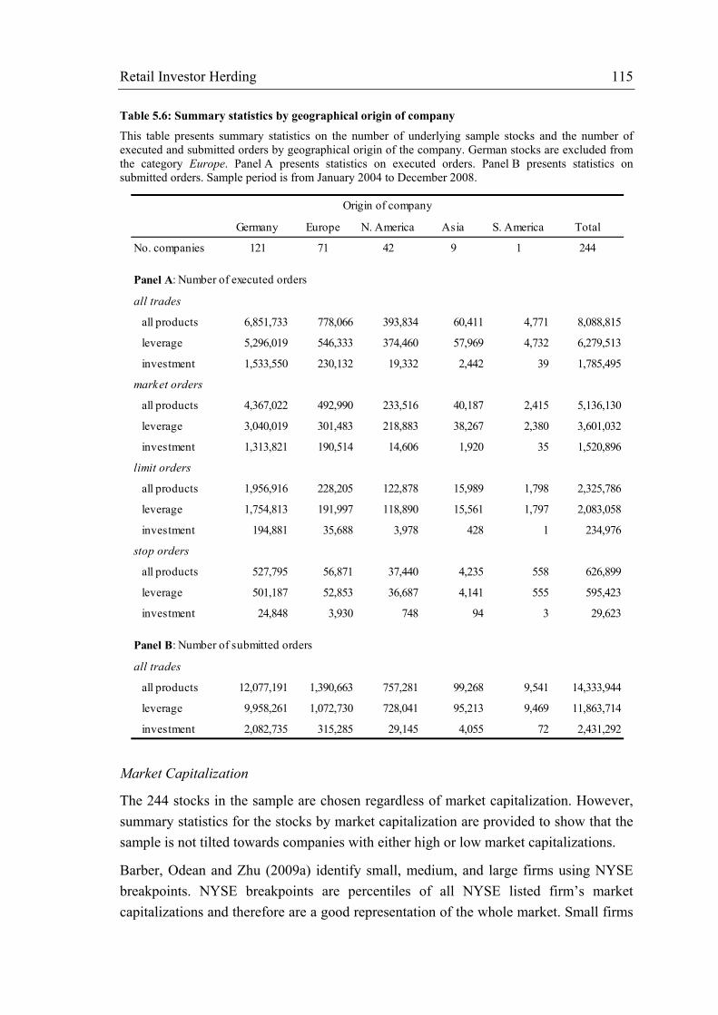
Retail Investor Herding 115
Table 5.6: Summary statistics by geographical origin of company
This table presents summary statistics on the number of underlying sample stocks and the number of executed and submitted orders by geographical origin of the company. German stocks are excluded from the category Europe. Panel A presents statistics on executed orders. Panel B presents statistics on submitted orders. Sample period is from January 2004 to December 2008.
Market Capitalization
The 244 stocks in the sample are chosen regardless of market capitalization. However, summary statistics for the stocks by market capitalization are provided to show that the sample is not tilted towards companies with either high or low market capitalizations.
Barber, Odean and Zhu (2009a) identify small, medium, and large firms using NYSE breakpoints. NYSE breakpoints are percentiles of all NYSE listed firm’s market capitalizations and therefore are a good representation of the whole market. Small firms
Germany Europe N. America Asia S. America Total
No. companies 121 71 42 9 1 244
all trades
all products 6,851,733 778,066 393,834 60,411 4,771 8,088,815
leverage 5,296,019 546,333 374,460 57,969 4,732 6,279,513
investment 1,533,550 230,132 19,332 2,442 39 1,785,495
market orders
all products 4,367,022 492,990 233,516 40,187 2,415 5,136,130
leverage 3,040,019 301,483 218,883 38,267 2,380 3,601,032
investment 1,313,821 190,514 14,606 1,920 35 1,520,896
limit orders
all products 1,956,916 228,205 122,878 15,989 1,798 2,325,786
leverage 1,754,813 191,997 118,890 15,561 1,797 2,083,058
investment 194,881 35,688 3,978 428 1 234,976
stop orders
all products 527,795 56,871 37,440 4,235 558 626,899
leverage 501,187 52,853 36,687 4,141 555 595,423
investment 24,848 3,930 748 94 3 29,623
all trades
all products 12,077,191 1,390,663 757,281 99,268 9,541 14,333,944
leverage 9,958,261 1,072,730 728,041 95,213 9,469 11,863,714
investment 2,082,735 315,285 29,145 4,055 72 2,431,292
Origin of company
Panel A: Number of executed orders
Panel B: Number of submitted orders

Retail Investor Herding 116
are those in their sample below the 30th percentile of NYSE market cap, while large firms are those above the 70th percentile.
Kaniel, Saar, and Titman (2008) define small, medium, and large capitalization stocks as stocks below the 40th percentile, between the 40th and the 70th percentiles, and above the 70th percentile, respectively. In contrast to Barber, Odean, and Zhu, they do not use an external source such as the NYSE breakpoints to validate their classification.
For the purpose of this study, the market capitalization of each stock in the sample is calculated at the beginning of each year (2004 to 2009), and the respective averages of the whole 5-year-period are computed. As breakpoints, 2 billion and 20 billion Euros are used. Small firms are defined as firms with an average market capitalization below 2 billion Euros, medium firms between 2 billion and 20 billion Euros, and large firms above 20 billion Euros. Table 5.7 shows median and mean values for market capitalizations in the respective categories. The classification almost divides the sample into three equally-sized groups of about 80 stocks.
Table 5.7: Summary statistics on market capitalization
This table presents the breakpoints for the market cap classification as well as the number of companies in the sample assigned to each group. The two columns on the right report the median and the mean market capitalization for each group.
Market capitalization statistics are used to test whether there are any differences in retail investor herding between small capitalization stocks and large capitalization stocks.
5.5.2. Herding Measure
The herding measure used in this section is very similar to the one used in Lakonishok, Shleifer, and Vishny (1992). The LSV measure, , is defined as
∑∑ ∑ | | (5.3)
where Nt is the number of stocks traded during period t, the buyers ratio is the number of net buyers of stock j during period t divided by the number of active traders of j during t, and the period-average buyers ratio is the number of net buyers aggregated across all stocks during period t divided by the number of all active traders during t.
Market capitalization (in million €)
No. companies in sample Median Mean
Small cap < 2,000 80 710 827
Medium cap 2,000 - 20,000 81 6,682 8,385
Large cap > 20,000 83 50,072 66,625

Retail Investor Herding 117
Subtracting the term controls for general shifts into or out of stocks that affects all stocks alike – for example due to an economic crisis or a stock market boom. The term | | is an adjustment factor that accounts for the statistical fact that the absolute value of is greater than zero even if there is no herding at all. For this reason, LSV calculate the expected value of | | using the binomial distribution and subtract this term from the empirically determined term . For any stock, however, the adjustment factor declines as the number of active traders in that stock rises.
The message of the LSV measure can be illustrated by an example as follows: Suppose there are 100 active traders of a stock during a certain period, and 60 of them are net buyers, i.e. during the period they buy more than they sell. As a result, the buyers ratio for this stock is 0.6. For all stocks traded in the same period, there are 1000 traders dividing into 500 net buyers and 500 net sellers resulting in a period-average buyers ratio of 0.5. The LSV measure for stock j in period t is then |0.6-0.5|=0.1 which means that 10% of all traders more than indicated by the period average are on the same side of the market.
The concept of the LSV measure cannot directly be transferred to this work’s data set because there is a major difference in the data: Since all orders are anonymous, i.e. it is not possible to determine whether two orders have originated from the same individual (though it is possible to determine the broker), a measure that is based on the number of individuals cannot be computed. Instead, the modified measure is based on the number of orders rather than the number of investors. Therefore, the measures should be equal if every order for each instrument is submitted by a different investor. Since this is not realistic there will be differences between the measures. However, the greater the dispersion of orders among retail investors, the smaller is the expected difference. In addition, there is no need for an adjustment factor in our measure due to the different calculation basis.
The herding measure used in this section is calculated as follows:
∑∑ ∑ (5.4)
∑ ·
∑ (5.5)
where Nt is the number of stocks with at least 5 executed orders in period t. This restriction on the minimum number of transactions per stock and time period ensures that a meaningful herding measure can be calculated. is the ratio of optimistic
investors as defined in section 5.3.2 for stock j and period t. is the average

Retail Investor Herding 118
optimistic investor ratio based on all stocks with the minimum number of orders in period t. It is weighted by the number of orders.
5.5.3. Results
The herding measure is calculated for different time periods (daily, weekly, monthly, and quarterly), different product types (all product types, leverage products, investment products), and different order types (all order types, market orders, limit orders). Table 5.8 presents the results.
Table 5.8: Modified LSV herding measure by product and order type
This table presents summary statistics for the measure. Statistics are reported for different time periods, different product types, and different order types.
Results include the mean, the median, the standard deviation and the number of observations. Note that the number of observations is a measure of the number of stock-period-measures with at least 5 trades in the respective underlying. For this reason,
numbers of sub categories do not add up to 100%.
The average daily herding measure on a stock level is 17% which means that on average 17% of all trades more than expected are on the same side of the market every day. This means that there is substantial herding also on the stock level.
Herding measures are lower for longer time periods: For example, the average quarterly herding measure on a stock level is 8.7% indicating that the longer time period smoothes the higher daily herding values and brings them back to a more moderate level. For a given quarter, trades on different days and on different sides are more likely to cancel each other out so the quarterly herding measure is not affected.
all leverage investment all leverage investment all leverage investmentDaily Mean 17.0% 17.5% 17.5% 16.9% 17.5% 17.2% 21.8% 22.1% 20.5% Median 14.3% 14.8% 14.6% 14.0% 14.7% 14.3% 19.2% 19.6% 16.9% Std. Dev. 12.9% 13.1% 13.7% 13.1% 13.3% 13.6% 15.4% 15.5% 15.6% Observations 147,591 131,798 56,882 118,854 100,531 51,134 79,978 74,481 13,472Weekly Mean 14.1% 14.3% 17.6% 14.5% 14.7% 17.6% 17.9% 18.1% 19.1% Median 11.4% 11.7% 14.7% 11.6% 11.8% 14.7% 15.5% 15.7% 16.1% Std. Dev. 11.2% 11.3% 13.9% 11.7% 11.8% 13.9% 13.0% 13.1% 14.6% Observations 46,377 44,311 24,699 42,809 39,535 22,491 35,938 33,981 10,274Monthly Mean 11.0% 10.7% 16.9% 11.6% 11.4% 17.1% 13.6% 13.6% 17.7% Median 8.5% 8.3% 14.1% 8.9% 8.7% 14.0% 11.2% 11.3% 15.0% Std. Dev. 9.3% 9.2% 13.5% 10.0% 10.0% 13.7% 10.6% 10.7% 13.6% Observations 11,796 11,689 8,597 11,599 11,397 8,098 11,190 10,961 5,304Quarterly Mean 8.7% 8.0% 15.3% 9.3% 8.5% 15.8% 10.3% 10.3% 16.1% Median 6.6% 6.0% 12.6% 7.2% 6.2% 12.9% 8.2% 8.2% 13.2% Std. Dev. 7.8% 7.5% 12.4% 8.4% 8.2% 12.9% 8.7% 8.7% 12.8% Observations 4,023 3,998 3,393 4,000 3,973 3,289 3,954 3,930 2,648
All Order Types Market Orders Limit Orders

Retail Investor Herding 119
Herding in investment products is higher than in leverage products: In each quarter, of all trades in investment products, 15.3% more than the average are on the same side of the market whereas the value is 8.0% for leverage products. This is a result of different time horizons of the products: Leverage products are flow products that are bought and sold within days whereas investment products are instruments that are likely to be held for months or even years.
Herding measured by limit orders is higher than by market orders. This is due to the automatic execution of limit orders as a result of market movements. The interesting part of the comparison, however, is the finding that herding measured by market orders is substantial and almost as high as the herding measured by limit orders: The average daily herding measure using market orders is 17.5% and the average quarterly herding measure equals 8.5%. These results prove that the herding found in the data is not only an artifact of the execution of stale limit orders.
Table 5.9 provides another view on the data. As a robustness check, herding measures are presented not only by product type but also by size of the underlying company. Market capitalization of each stock is determined at the beginning of each year (2004 to 2009) and the respective averages of the whole 5-year-period are computed. 2 billion and 20 billion Euros are used as the size breakpoints as explained in section 5.5.1.
Table 5.9: Modified LSV herding measure by firm size
This table presents summary statistics for the measure. Statistics are reported for different time periods, different product types, and different firm sizes.
On a daily basis, average herding in small stocks is higher than average herding in large stocks. This difference is statistically significant as a t-test on the time series means
all leverage investment all leverage investment all leverage investmentDaily Mean 18.2% 18.8% 21.8% 16.4% 16.9% 18.5% 16.9% 17.3% 15.7% Median 15.6% 16.2% 19.9% 13.8% 14.3% 16.0% 13.9% 14.3% 12.6% Std. Dev. 13.4% 13.6% 14.9% 12.4% 12.6% 13.7% 13.1% 13.3% 13.0% Observations 37,597 34,376 6,389 54,938 51,078 22,673 55,056 46,344 27,820Weekly Mean 14.7% 15.0% 20.1% 13.2% 13.4% 17.6% 14.4% 14.6% 16.3% Median 12.1% 12.6% 17.7% 10.8% 11.0% 15.0% 11.5% 11.7% 13.1% Std. Dev. 11.4% 11.6% 14.5% 10.6% 10.6% 13.7% 11.5% 11.7% 13.5% Observations 12,348 11,922 5,447 15,949 15,555 9,371 18,080 16,834 9,881Monthly Mean 11.1% 11.2% 18.8% 10.3% 10.0% 16.3% 11.4% 11.0% 16.2% Median 8.7% 8.9% 15.8% 7.9% 7.7% 13.7% 9.0% 8.7% 13.1% Std. Dev. 9.5% 9.5% 14.0% 9.0% 8.8% 13.0% 9.4% 9.3% 13.3% Observations 3,161 3,123 2,354 4,040 4,023 2,951 4,595 4,543 3,292Quarterly Mean 8.8% 8.6% 16.4% 8.1% 7.4% 15.0% 9.2% 8.0% 14.7% Median 6.7% 6.6% 14.1% 6.1% 5.6% 12.3% 7.0% 6.0% 11.8% Std. Dev. 8.1% 8.2% 12.4% 7.4% 7.1% 12.4% 8.0% 7.2% 12.4% Observations 1,088 1,079 945 1,372 1,370 1,124 1,563 1,549 1,324
Small Caps Mid Caps Large Caps

Retail Investor Herding 120
involving all instruments shows (p-value < 0.0001). On a weekly basis, herding in smaller stocks is still higher than herding in large stocks though not as significant. The t-test on the weekly time series averages shows that the time series are different with a p-value of 0.048, i.e. at the 5% level. When looking at longer periods, this difference reverses: For monthly and quarterly time series, herding is higher in large stocks than in small stocks. However, differences in the weekly and quarterly time series are not statistically significant.
On a quarterly level, this result is seemingly contrary to the result reported in Lakonishok, Shleifer, and Vishny (1992): They find greater herding in small stocks and argue that intentional herding should indeed be higher in small stocks since institutionals follow each other’s actions more closely when public information is not widely available.
On a daily level, however, the significant difference between the small and large cap time series can be explained similarly: Since small capitalization stocks usually receive less attention than large capitalization stocks, investors are more likely to react similarly and simultaneously to the same news and price movements. On a daily basis, this behavior leads to a higher herding measure. For large capitalization stocks, information is widely available and opinions of retail investors are more likely to be different and so trades can cancel each other out.
5.5.4. Review of Results
Overall, the magnitudes of our modified herding measure values are similar to those reported by other recent studies (see Table 5.10 for a comparison):
Grinblatt, Titman, and Wermers (1995) find an overall fund herding measure of 0.84 meaning that a fund that traded 10 percent of its portfolio each quarter bought stocks that had about 8.4 percent excessive buying by all funds, or sold stocks that had about 8.4 percent excessive selling. This is equivalent to the value found in quarterly herding (8.7%) in the Euwax data set.
Dorn, Huberman, and Sengmueller (2008) calculate LSV measures for a German discount broker, and their monthly results come very close to those for the discount broker in the study by Barber, Odean, and Zhu (2009b). They do find, however, that herding in the more liquid stocks of the DAX30 is almost twice as high as herding in all stocks taken together – a finding that cannot be confirmed. However, the herding levels found for large cap stocks in the Euwax data set closely match the findings of Dorn, Huberman, and Sengmueller: Both studies show an 11.4% herding level. This close match confirms the findings for large cap stocks.
Barber, Odean and Zhu (2009b) calculate monthly LSV herding measures and find that they are reliably positive for both their datasets (a retail broker and a discount broker).

Retail Investor Herding 121
They find that herding measure values at the retail brokerage are more than double of those at the discount brokerage. Their values (6.8% and 12.8%, respectively) are similar to the monthly Euwax herding measure (11%) considering that the data incorporates discount brokers as well as traditional retail brokerages. Barber, Odean and Zhu also differentiate firms of different sizes but do not find a consistent difference in the results when distinguishing firms by market capitalization. This finding is in line with the monthly results reported in this section.
Table 5.10: Comparison of LSV measures across studies
In this table, average monthly herding measures found in different studies are compared to each other. The bottom line reports average monthly UHM values based on the number of executed orders.
To sum up, herding in single underlyings by retail investors is high and substantial. In addition, although there are methodological differences, the herding measure developed in this section is comparable to other herding measures in the relevant literature, and they are similar in value. The magnitude of herding does not change when controlling for firm size (market capitalization). Herding is higher for limit orders than for market orders due to the automatic execution of limit orders.
5.6. Conclusion In this chapter, retail investor herding in securitized derivatives is examined using order data from the European Warrant Exchange. A herding measure is constructed that allows for the detection of retail investor herding on a market-wide level as well as a stock-level.
The results show that substantial retail investor herding exists on the market level and that the degree of herding is closely related to the use of limit and market orders as well as overall market conditions. Bearish periods are characterized by an overall injection of capital by retail investors. The level of herding in bear markets is generally higher than in bull markets. This result holds for limit as well as market orders. Pessimistic herding is higher in bull markets than in bear markets, and optimistic herding is higher in bear
Study all sizes small medium largeBarber, Odean, and Zhu (2009b)
Discount Broker 6.8% 7.6% 6.6% 5.4%Retail Broker 12.8% 11.4% 13.1% 12.5%
Dorn, Huberman, and Sengmueller (2008) 6.4% n/a n/a n/aDAX30 stocks 11.4%
Grinblatt, Titman, and Wermers (1995) 8.4% n/a n/a n/a
this study 11.0% 11.1% 10.3% 11.4%

Retail Investor Herding 122
markets than in bull markets. Together, these results support the hypothesis that retail investors are contrarian. Mechanical execution of limit orders alone cannot explain this phenomenon.
By measuring herding on a broker level, the question is answered whether herding is an aggregate phenomenon or whether it can be observed for the order flows of individual brokers. Substantial herding of retail investors is observed across all brokers: The level is highest among public brokers with a rather conservative clientele and lowest among online brokers that neither give investment advice nor operate any branches. Proprietary brokers do not seem to fit into the same schema as they exhibit very different trading patterns.
In addition to market-wide herding, the results show that retail investors also herd into and out of single underlyings: Excess herding is substantial and significant, meaning that retail investors choose the same underlying securities with a probability that is higher than expected by chance. This result is neither fully explained by the use of limit orders, nor by retail investors’ focus on small firms. On a daily basis, however, herding is higher in small firms than in large firms meaning that small firms tend get the attention of retail investors at the same time.
To put these results into the larger context of retail investor behavior and price formation, it has to be concluded that retail investor trading is highly correlated and as a whole, retail investors may have the potential to actually affect stock prices.

The Predictive Power of Retail Investor Sentiment 123
6 The Predictive Power of Retail Investor Sentiment
“In general, the contrarian behavior we document of individual investors on the NYSE seems important for understanding short-horizon return predictability.”
Kaniel, Saar, and Titman (2008), p. 306
The contrarian behavior of individual investors, as documented in the previous chapter, may present a link to stock return predictability as suggested by Kaniel, Saar, and Titman. They find that individual investors are contrarians implicitly providing liquidity to other market participants and that their behavior may predict returns.
The central goal of this chapter is to determine whether it is possible to successfully use sentiment data – the Euwax Sentiment measures in particular – in trading strategies to generate abnormal returns, i.e. returns in excess of known risk factors and above market returns. In this chapter, a trading strategy involving single underlyings is being developed that consists of buying high sentiment stocks and selling low sentiment stocks resulting in a zero-cost portfolio. In the course of the chapter, the influence of product and order types is being discussed as well as the difference between using executed and submitted orders.
The results show that the returns of the zero-cost portfolio are significantly positive even after controlling for market returns and momentum. Controlling for firm size reveals that sentiment only predicts returns for small firms whereas there is no predictive quality for medium and large capitalization firms. This is in line with theoretical results of small investor research.
The chapter is structured as follows: In section 0, related work with respect to order imbalance measures is presented and discussed in detail. Section 6.2 provides an overview of the data set. Section 6.3 is the main section of this chapter. It contains the description of the methodology, the results as well as the description of control variables. Section 6.4 adds some robustness checks. Section 6.5 concludes this chapter.

The Predictive Power of Retail Investor Sentiment 124
6.1. Related Work There is a growing body of literature that examines the dynamic relationship between investor sentiment and contemporaneous as well as future stock returns. These studies typically use indirect sentiment measures such as order flow data, put/call ratios, and buy/sell imbalances, and relate them to stock returns.
Jackson (2003) analyzes a unique dataset of individual investor trades in Australia and examines whether the investment decisions of individual investors aggregate in a systematic way. He finds that the aggregation assumption holds across 56 unrelated brokerage firms, across sub-periods, and across subsets of stocks. Regarding the relationship between individual investor trading and future stock returns, he finds that net trades (buy minus sell volume) of full-service brokerage clients positively and significantly forecast future short-term market and cross-sectional returns. Similar to Jackson (2003), Barber, Odean, and Zhu (2009b) show that the trading of individual investors at a large discount brokerage and a large retail brokerage is systematically correlated. Using another brokerage data set from the U.S., Kumar and Lee (2006) show that retail investor trades are systematically correlated and retail investors buy and sell stocks in concert. Moreover, they find that monthly changes in retail sentiment induce co-movement in stock returns.
Baker and Stein (2004) use trading volume as a measure of liquidity which can also be interpreted as a measure of investor sentiment. They identify short-selling as a problem and assume that investors generally only invest when they are optimistic and thereby assume that investors reduce liquidity as they become more pessimistic. In their data, they find a negative relation between annual turnover and subsequent annual stock returns suggesting that irrational investors overreact and cause stock prices to revert.
Pan and Poteshman (2006) analyze option trading data and construct open-buy put-call ratios from option volume initiated by buyers to open new positions. When comparing the predictability of the other option volume types (open sell, close buy, close sell) they find that they do predict the correct direction but to a much lower extent than the open buy volume. Using this non-publicly available put-call ratio and publicly observable option volume, Pan and Poteshman examine the predictability of option trading for future stock price movements. They find that the open-buy put-call ratio positively predicts future stock prices on a weekly horizon.
Kaniel, Saar, and Titman (2008) examine individual investors’ trading behavior using a unique dataset from the New York Stock Exchange that contains the aggregate volume of executed buy and sell orders of individual investors over four years. Very similar to the methodology applied in this work, they define individual investors’ net trading as the difference between buy and sell volume. They find that the trades of individual

The Predictive Power of Retail Investor Sentiment 125
investors can indeed be used to systematically forecast stock returns and show that statistically significant positive payoffs can be realized using this information.
In a similar study, Barber, Odean, and Zhu (2009a) use TAQ/ISSM data to investigate the effect of order imbalance of individual investors. Like several previous studies, they document strong herding by individual investors. Over shorter periods, they find that stocks heavily bought by individual investors in one week earn strong returns in the subsequent week, while stocks heavily sold in one week perform poorly in the subsequent week. Over longer periods, however, Barber, Odean, and Zhu document that stocks with small-trade selling pressures outperform those with buying pressures, indicating a negative relationship between investor sentiment and stock returns at longer horizons.
Using the same data set, Hvidkjaer (2008) shows that stocks with intense sell-initiated small-trade volume, measured over several months, outperform stocks with intense buy-initiated small-trade volume. His findings support the role of retail investor sentiment as a contrary indicator for long-term stock price movements and positively relate to those of Barber, Odean, and Zhu. In a paper similar in spirit, Frazzini and Lamont (2008) study the effect of mutual fund flows on stock returns and find that stocks favored by retail investors tend to underperform in subsequent years.
Using the dataset of a large German discount broker, Dorn, Huberman, and Sengmueller (2008) show that retail investors tend to be on the same side of the market in a given stock. They argue that aggregated market orders lead returns whereas aggregated limit orders appear to be negative feedback trades. They point out that the distinction between market and limit orders is crucial for understanding the relation between individual investor trading and returns.
Schmitz, Glaser, and Weber (2007) identify warrant trades as an effective measure of sentiment. Their data is collected from a German discount broker and includes the portfolio data of a large number of investors. They calculate a simple sentiment measure using investors’ warrants holdings. Investors that only hold calls (puts) are classified as optimistic (pessimistic), and investors that hold both are classified as neutral.
Discussion
The evidence on the relationship between individual investor trading seems to differ depending on three dimensions that distinguish the different studies: (i) the horizon of the relationship, (ii) the underlying data set (trades, transactions, instruments, etc.), and (iii) the method of aggregating the data.
Concerning the horizon, all of the studies above document a positive relation of individual investor sentiment and future stock returns on a daily or weekly level, whereas many of the studies find a negative relation on much longer horizons, i.e.

The Predictive Power of Retail Investor Sentiment 126
months and years. Of course, the availability of high-frequency data has improved considerably in the last couple of years so that short-horizon relations were difficult to detect in earlier studies.
The underlying data sets also differ in a couple of important dimensions: First, there are two major sources for transaction data: exchange data with executed transactions for a whole market, and brokerage data with trades and portfolio information on an individual account level. The brokerage data has the advantage that trading decisions can be traced to individual accounts, and individual portfolios can be reconstructed. The exchange data usually does not contain information about individuals but contains trades from multiple brokerages and therefore allows for the distinction of different order flows. A second dimension is the differentiation of trade direction: Some of the papers rely on algorithms such as the one proposed by Lee and Ready (1991) to infer buyer- or seller-initiated trades, others use unique data sets where the trade direction is part of the data. The third dimension is the problem of disentanglement. Disentanglement is the act of separating institutional transactions from retail investor transactions. Some studies use retail brokerage data sets where all trades are supposed to come from retail investors, others rely on the small-trade volume or low-market-capitalization stocks. Fourth, the country of origin may be of importance since investors in Taiwan may act differently from those in the U.S. or in Germany. A fifth aspect concerns whether it is possible for retail investors to express negative sentiment. A retail investor has two practical alternatives in the equity market when trying to express a negative investor sentiment. They have the option to sell stock currently held, or if they already hold nothing they can decide not to buy. The option to sell stock short is practically impossible due to margin requirements, short-sell restrictions, and levels of investor knowledge. This severely limits a retail investor’s ability to express a negative sentiment, and so an important part of the whole picture may be missing.
The aggregation methodology across the literature has similarities but differs in certain aspects: Studies based on market data usually use order flow data of executed transactions and aggregate them creating measures of imbalance for buy and sell decisions, put and call volumes, small trades and large trades, etc. There are many possible ways to construct a sentiment measure out of order flow data, and many of them are highly correlated.
In this chapter, most of the weaknesses mentioned above are addressed and avoided by using a data set that (i) consists of retail investor orders only, (ii) captures orders from different brokerages, (iii) includes the explicit trade direction due to the market model and (iv) allows for the expression of negative sentiment through put options.

The Predictive Power of Retail Investor Sentiment 127
6.2. Data and Methodology In addition to market-wide retail investor sentiment as explored in chapter 4 there is the possibility to calculate retail investor sentiment individually for single stocks. A large number of covered warrants and investment certificates is based on single stocks as underlyings. Sentiment measures for individual stocks have the advantage that they can be compared across all stocks and thereby sorted by value. At one point in time, it is possible to sort all stocks according to their sentiment value. This methodology has the advantage that only extreme values with unambiguous interpretation are used whereas values with no clear conclusion can be omitted.
6.2.1. Data Set
In the data base, 37% of all customer orders comprise securitized derivatives with individual stocks as underlying value (see Table 4.1 on page 77, Panel C). The underlying stocks comprise global companies with a focus on European and especially German companies. This is not surprising since EUWAX and most of its customers are based in Germany. Trading intensity and frequency vary across all instruments. While there are on average more than 10,000 executed orders per month on underlyings such as Allianz, Daimler, and Deutsche Telekom, there are also stocks that do not receive such a high attention. There are stocks in the data base with less than 10 executed orders in related derivative instruments during the whole time period of five years.
The calculation of a sentiment measure based on executed or submitted orders demands that there is a minimum amount of trading in related instruments otherwise such a measure cannot be calculated. Therefore, all underlying stocks are filtered by employing the following methodology22: All underlyings are sorted according to the average number of executed orders per month. As a rule of thumb, an average trading amount of 3 executed orders per day is demanded resulting in 60 executed orders per month (assuming 20 trading days per month). This filter is applied to all underlyings and results in 244 stocks comprising about 97% of all executed trades on stocks in the data base.
Summary statistics on the number of executed and submitted orders are presented in Table 5.6 on page 115. About half of the stocks that serve as underlyings for the derivatives in the sample are German stocks, almost 30% are other European stocks, and the rest is from North and South America as well as Asia. In addition, the number of all executed as well as submitted orders by geographical region as well as product and order type is shown. The overall relation of executed to submitted orders by product type is shown in Table A.2 in the appendix (Panel C).
22 The same methodology as in section 5.5.1 is used.

The Predictive Power of Retail Investor Sentiment 128
The 244 stocks in the sample are chosen regardless of market capitalization. Summary statistics by market capitalization are provided in Table 5.7 on page 115 to show that the sample is not tilted towards companies with either high or low market capitalizations. As explained in section 5.5.1, small firms are defined as firms with an average market capitalization below 2 billion Euros, medium firms between 2 billion and 20 billion Euros, and large firms above 20 billion Euros. The classification divides the sample in three almost equally-sized groups of about 80 stocks.
Market capitalization statistics are used later in this chapter to test whether there are any differences between small capitalization stocks and large capitalization stocks in how retail investor sentiment predicts returns.
6.2.2. Methodology
In this section a portfolio trading strategy23 is implemented that consists of buying stocks when their respective sentiment measures are high and selling stocks when sentiment measures are low. The idea behind this portfolio methodology is to focus on stocks with extreme (positive and negative) sentiment values and disregard the stocks with sentiment values in between.
Two portfolios are constructed: One portfolio, the high sentiment portfolio, includes the highest decile of stocks that have the highest sentiment values on the portfolio formation day. The other portfolio, the low sentiment portfolio, includes the lowest decile of stocks with the lowest sentiment values. Throughout this section, sentiment values based on the number of executed orders are used for portfolio construction (instead of the volume based sentiment values) as Chapter 4 has shown that this measures yields better results. Robustness checks later in this chapter come to the same conclusion.
The returns of a long-short strategy that involves buying the high sentiment portfolio and selling the low sentiment portfolio are calculated, henceforth referred to as the high-low sentiment portfolio.
Two periods in general are differentiated: the portfolio formation period and the portfolio holding period. The portfolio formation period comprises all trading days over which sentiment values are being aggregated. For example, a portfolio formation period of one means that sentiment values are calculated based on the last trading day whereas a portfolio formation period of five means that sentiment values are derived from all trades in the last five trading days. The portfolio holding period determines how long the respective portfolios are being held. Returns are then cumulated using the sum of logarithmic returns of the single holding days after portfolio formation. 23 Jackson (2003), Pan and Poteshman (2006), Kaniel, Saar, and Titman (2008), Dorn, Huberman, and Sengmueller (2008), and Barber, Odean, and Zhu (2009a) use similar portfolio construction methodologies.

The Predictive Power of Retail Investor Sentiment 129
Day t=0 is regarded as the last day of the portfolio formation period which means that t=1 would be the first day of the portfolio holding period. Returns for day 1 would be calculated using the end-of-day logreturns from day 0 to day 1. To illustrate this, consider the following example for a one-day portfolio formation and a one-day portfolio holding period: On Monday (t=0), shortly before the end of the trading day, sentiment values for all stocks are being calculated and sorted, and high and low sentiment portfolios are being formed. All stocks are being bought just before the end of trading and held for exactly one day and finally sold on Tuesday (t=1) right before the end of trading. The return of the portfolio is expressed as the average of all logreturns calculated using the respective closing prices of all stocks in the portfolio.
Not all stocks in the sample are being considered for inclusion in the portfolios. To be eligible for the portfolio formation procedure, underlying instruments must have at least 3 executed orders per day during the portfolio formation period on average. This prevents stocks from getting high sentiment ranks when there are only 1 or 2 orders per day.24
6.3. Results This section presents the results of the cross-sectional portfolio formation analysis. Sentiment deciles are used to capture only extreme sentiment. Sentiment measures based on the number of executed orders are chosen to be invariant against extremely high volumes, outliers, and potential errors in the data set. In addition, the following sections use a one-day portfolio formation period (i.e. portfolios are formed on day t=0). Variations of this are considered in additional robustness checks.
Other parameters, such as product type or order type, are varied throughout the rest of this section to investigate the different effects of these parameters on the results. Additional robustness checks are reported in section 6.4.
6.3.1. Pre- and Post Portfolio Formation Returns
Product type
Table 6.1 shows daily average portfolio logreturns for five days before and five days after the portfolio formation day. As explained in the previous section, portfolios are formed according to sentiment values in t=0, and their returns are observed for days t=-5 to t=5. Returns are expressed in basis points.
24 Additional robustness checks (not reported) have shown that setting the minimum number of orders to 5 or 10 does not change the portfolio formation significantly.

The Predictive Power of Retail Investor Sentiment 130
Table 6.1: Return statistics by product type
This table presents average portfolio logreturns for a 5-day pre- and post-portfolio-formation period. The low sentiment portfolio includes stocks with the lowest sentiment values on the day of portfolio formation (t=0). The high sentiment portfolio includes stocks with the highest sentiment on the day of portfolio formation. The high-low excess portfolio is constructed by selling the low sentiment portfolio and buying the high sentiment portfolio. The p-values in brackets show the statistical significance of a t-test that tests whether the excess returns are different from zero. Results are shown for sentiment based on different product types.
Using all product types, i.e. sentiment values based on leverage and investment products, average low sentiment portfolio returns are negative for days t=1 to t=5 whereas high sentiment portfolio returns are positive for the first five trading days after portfolio formation. Taken together, the high-low sentiment portfolio excess returns that are the result of a long-short strategy using these two portfolios yield statistically and economically significantly positive returns for at least the first five trading days after portfolio formation. p-values indicate that the excess returns are significantly different from zero.
Product types are differentiated in order to determine the driver behind the positive excess returns. Using leverage products only, the same pattern can be observed: There are highly negative low sentiment portfolio returns and highly positive high sentiment portfolio returns that yield significantly positive excess returns. Sentiment portfolios based on investment products do not exhibit these return patterns. This indicates that any predictive power that may be a result of the sentiment portfolio construction can be attributed to retail orders in leverage products.
The results suggest that on the day of portfolio formation (t=0) investors on average act as contrarian traders being pessimistic about stocks that experience high returns and
-5 -4 -3 -2 -1 0 1 2 3 4 5
All products
Low Sentiment Portfolio Returns 12.4 14.6 14.0 19.1 29.8 56.9 -6.4 -6.3 -2.9 -3.8 -1.7
High Sentiment Portfolio Returns -17.9 -17.6 -18.8 -25.8 -35.5 -55.9 3.8 2.5 0.9 4.8 1.8
High-Low Portfolio Excess Returns -30.3 -32.2 -32.8 -44.8 -65.4 -112.7 10.2 8.8 3.7 8.7 3.5
p-value (0.000) (0.000) (0.000) (0.000) (0.000) (0.000) (0.000) (0.000) (0.088) (0.001) (0.086)
Leverage products
Low Sentiment Portfolio Returns 11.8 13.6 16.5 21.8 33.6 64.3 -6.8 -6.7 -5.4 -4.8 -1.9
High Sentiment Portfolio Returns -20.5 -20.5 -22.8 -27.8 -40.1 -63.5 3.2 1.7 -2.2 1.8 2.1
High-Low Portfolio Excess Returns -32.3 -34.1 -39.3 -49.6 -73.7 -127.8 10.0 8.4 3.2 6.6 4.0
p-value (0.000) (0.000) (0.000) (0.000) (0.000) (0.000) (0.001) (0.001) (0.125) (0.012) (0.077)
Investment products
Low Sentiment Portfolio Returns 5.5 9.5 8.8 10.0 17.8 23.4 -1.5 -5.1 -1.5 -2.3 -1.4
High Sentiment Portfolio Returns -8.9 -13.4 -15.3 -12.0 -19.1 -31.6 -1.2 1.7 -1.9 0.3 -3.8
High-Low Portfolio Excess Returns -14.4 -22.9 -24.1 -22.0 -36.9 -55.1 0.3 6.8 -0.3 2.6 -2.5
p-value (0.000) (0.000) (0.000) (0.000) (0.000) (0.000) (0.463) (0.039) (0.466) (0.253) (0.231)
Return Day

The Predictive Power of Retail Investor Sentiment 131
being optimistic about stocks that experience low returns. In the case of the leverage products sentiment portfolios, stocks in the low sentiment portfolio experience an average daily return of 64.3 basis points whereas stocks in the high sentiment portfolio yield a loss of about the same amount (-63.5 basis points).
One possible explanation for these results is the automatic execution of stale limit orders that are in the order book for a long period and wait for their execution. Finally, when the market experiences a down- or an upturn, they are being executed automatically without any action by investors. It is therefore questionable to regard any extremely positive or negative sentiment values as real and especially timely investor sentiment (Linnainmaa (2009) elaborates on this).
Dorn, Huberman, and Sengmueller (2008) caution that “a failure to separate market and limit orders would lead us to classify retail investors as contrarian” and that “the mechanical correlation between limit order execution and returns masks the previously undocumented relations between speculative trading and returns” (p. 888). In order to determine whether the contrarian behavior is purely a result of limit order execution, the differentiation between order types is investigated in detail, i.e. the differentiation between limit and market orders.
Order type
For this purpose, each order is classified into two order types: limit orders which are not executed immediately, and market orders which also comprise marketable limit orders that are executed within 60 seconds of order submission (see section 4.2). There are two reasons why this rule is applied to distinguish limit orders from marketable limit orders: First, the data set does not include intraday reference prices that indicate whether a limit order was executable at the time of submission. Second, due to the market model at Boerse Stuttgart, even market orders may not be executed immediately but rather wait some seconds before the quality liquidity provider starts the execution process.
As in the previous section, results are shown for sentiment portfolios based on the different product types. Furthermore, Table 6.2 distinguishes between limit and market orders. Panel A shows the portfolio returns for sentiment portfolios based on sentiment that is constructed using limit orders only. The influence of limit orders can thereby be isolated.

The Predictive Power of Retail Investor Sentiment 132
Table 6.2: Return statistics by order and product type
This table presents average portfolio logreturns for a 5-day pre- and post-portfolio-formation period. The low sentiment portfolio includes stocks with the lowest sentiment values on the day of portfolio formation (t=0). The high sentiment portfolio includes stocks with the highest sentiment on the day of portfolio formation. The high-low excess portfolio is constructed by selling the low sentiment portfolio and buying the high sentiment portfolio. The p-values in brackets show the statistical significance of a t-test that tests whether the excess returns are different from zero. Panel A presents results based on sentiment created only from limit orders. Panel B presents results based on sentiment created from market orders.
The portfolio construction based on limit orders shows the expected results: On the day of portfolio formation, returns are positive for low sentiment stocks and negative for high sentiment stocks. Low sentiment stocks experience an average increase of 162
Panel A: Limit Orders
-5 -4 -3 -2 -1 0 1 2 3 4 5
All products
Low Sentiment Portfolio Returns 10.9 14.4 15.2 22.2 58.4 162.0 -0.7 -6.4 -4.5 -3.3 -2.8
High Sentiment Portfolio Returns -13.0 -12.4 -13.2 -19.3 -48.1 -130.1 -6.1 5.7 1.1 -0.8 -1.0
High-Low Portfolio Excess Returns -23.9 -26.8 -28.4 -41.6 -106.5 -292.1 -5.4 12.2 5.6 2.5 1.8
p-value (0.000) (0.000) (0.000) (0.000) (0.000) (0.000) (0.053) (0.000) (0.038) (0.218) (0.288)
Leverage products
Low Sentiment Portfolio Returns 10.1 13.3 14.8 22.8 58.7 165.4 -0.6 -8.0 -3.6 -3.9 -2.6
High Sentiment Portfolio Returns -16.2 -12.5 -13.2 -20.8 -51.0 -131.6 -6.9 4.5 -1.6 -1.7 -0.1
High-Low Portfolio Excess Returns -26.3 -25.8 -28.0 -43.6 -109.7 -297.0 -6.3 12.5 2.0 2.1 2.4
p-value (0.000) (0.000) (0.000) (0.000) (0.000) (0.000) (0.032) (0.000) (0.279) (0.257) (0.233)
Investment products
Low Sentiment Portfolio Returns 5.5 7.2 12.7 13.8 40.4 92.5 2.2 -4.9 -9.5 -5.5 -5.0
High Sentiment Portfolio Returns -12.7 -17.4 -15.8 -14.3 -38.0 -102.2 -1.5 5.2 -4.7 -5.9 5.6
High-Low Portfolio Excess Returns -18.2 -24.6 -28.5 -28.1 -78.4 -194.7 -3.7 10.1 4.8 -0.5 10.6
p-value (0.004) (0.000) (0.000) (0.000) (0.000) (0.000) (0.294) (0.051) (0.196) (0.459) (0.020)
Panel B: Market orders
-5 -4 -3 -2 -1 0 1 2 3 4 5
All products
Low Sentiment Portfolio Returns 8.9 10.4 12.1 15.3 21.4 30.3 -10.4 -5.4 -2.3 -4.3 0.0
High Sentiment Portfolio Returns -13.5 -13.3 -15.6 -20.7 -26.5 -36.5 4.4 0.5 -0.5 2.2 0.4
High-Low Portfolio Excess Returns -22.4 -23.7 -27.7 -36.0 -47.8 -66.8 14.9 5.9 1.8 6.5 0.3
p-value (0.000) (0.000) (0.000) (0.000) (0.000) (0.000) (0.000) (0.017) (0.255) (0.012) (0.450)
Leverage products
Low Sentiment Portfolio Returns 9.6 9.6 11.0 19.3 24.0 36.2 -11.0 -6.9 -3.6 -6.2 -1.8
High Sentiment Portfolio Returns -14.0 -14.9 -18.7 -22.4 -30.1 -45.0 7.8 -1.6 -3.7 1.1 0.9
High-Low Portfolio Excess Returns -23.5 -24.5 -29.7 -41.8 -54.1 -81.2 18.8 5.3 -0.1 7.3 2.7
p-value (0.000) (0.000) (0.000) (0.000) (0.000) (0.000) (0.000) (0.032) (0.491) (0.006) (0.188)
Investment products
Low Sentiment Portfolio Returns 7.1 9.8 6.1 8.7 15.8 16.0 0.7 -5.5 0.5 -0.9 -1.1
High Sentiment Portfolio Returns -11.6 -11.9 -13.7 -15.8 -17.0 -15.7 -0.8 5.0 -2.6 2.3 -1.9
High-Low Portfolio Excess Returns -18.6 -21.7 -19.8 -24.5 -32.8 -31.8 -1.5 10.5 -3.1 3.2 -0.8
p-value (0.000) (0.000) (0.000) (0.000) (0.000) (0.000) (0.344) (0.002) (0.174) (0.195) (0.410)
Return Day
Return Day

The Predictive Power of Retail Investor Sentiment 133
basis points, i.e. 1.62% on a single day whereas high sentiment stocks decline in value by 130.1 basis points on average. This phenomenon can be observed across product types although sentiment portfolios based on investment products alone exhibit lower absolute return values. This can be explained by the different investment horizons of leverage and investment products. Obviously, leverage product investors are more sensitive to contemporary price changes than investors seeking a longer term investment.
The results in panel A of Table 6.2 show that the influence of limit orders on sentiment values makes retail investors look as if they indeed behaved as contrarians. However, the same pattern can be observed in panel B of Table 6.2 when using sentiment portfolios constructed from market orders: Investors tend to submit market buy orders when stocks are declining in value on the same day and market sell orders when stock prices are rising. This behavior is contrarian, and it is not due to the automatic execution of limit orders.
Although portfolio returns on day t=0 suggest a contrarian behavior for market as well as limit orders, there are two important differences. Firstly, portfolio returns based on market order sentiment are not as high as portfolio returns based on limit order sentiment. Secondly, and more importantly, returns on day t=1 are different. Using limit orders for sentiment construction, portfolio returns for the low as well as the high sentiment portfolio are both negative (-0.6 and -6.3 basis points for leverage products), whereas portfolio returns for the high sentiment portfolio are positive (7.8 bp for leverage products) when using market orders for sentiment construction.
The long-short strategy based on sentiment constructed from market orders in leverage products would yield 18.8 basis points on the first day after portfolio formation (t=1) and 5.3 basis points on the second. Both are statistically significant.
Executed vs. submitted orders
Since the automatic execution of limit orders is an important factor in the sentiment construction and obviously influences the relation between sentiment and returns, the difference between submitted orders and executed orders is investigated. Submitted orders include all orders that have been submitted or changed and resubmitted, separately by product type but regardless of order type. The distinction between different order types is not necessary because the number of submitted market orders should equal the number of executed market orders already analyzed. In addition, the date of submission should equal the date of execution. Therefore, no distinction regarding the order type is made. Table 6.3 shows the results by product type.

The Predictive Power of Retail Investor Sentiment 134
Table 6.3: Return statistics for submitted orders
This table presents average portfolio logreturns for a 5-day pre- and post-portfolio-formation period. Sentiment values used for portfolio formation are based on the number of submitted orders. The p-values in brackets show the statistical significance of a t-test that tests whether the excess returns are different from zero. Results are shown for sentiment based on different product types.
The most notable findings are the following: First, contrarian behavior can be observed on day t=0 with sentiment data on submitted orders as well. Low sentiment portfolios experience relatively high returns whereas high sentiment portfolios experience relatively low returns. Second, in contrast to the results based on executed orders, absolute returns on the day of portfolio formation are lower than on the day before portfolio formation. Third, and most importantly, on the first four days after portfolio formation, the high-low sentiment portfolio yields statistically and economically significantly positive returns: On the first day, it yields 15.6 basis points, followed by 7.5 bp, 5.4 bp, and 4.7 bp. This result is primarily driven by leverage products: Portfolio returns based on leverage product sentiment are even higher, yielding 15.6 bp, 7.4 bp, 6.4 bp, and 5.0 bp, all statistically significant at the 5% level.
To summarize, a portfolio of stocks that retail investors are optimistic about develops well during the next four trading days, whereas a portfolio of stocks that retail investors are pessimistic about experiences negative returns on the days after order submission.
6.3.2. Control Variables
In order to attribute any portfolio returns to retail investor sentiment, known effects have to be controlled for and thereby excluded. For example, results have to be
Submitted Orders-5 -4 -3 -2 -1 0 1 2 3 4 5
All products
Low Sentiment Portfolio Returns 12.5 11.8 15.3 18.4 22.9 9.8 -8.3 -4.0 -3.1 -0.9 1.7
High Sentiment Portfolio Returns -19.4 -22.5 -21.5 -26.9 -30.6 -17.7 7.2 3.6 2.3 3.8 0.1
High-Low Portfolio Excess Returns -32.0 -34.3 -36.9 -45.3 -53.6 -27.5 15.6 7.5 5.4 4.7 -1.6
p-value (0.000) (0.000) (0.000) (0.000) (0.000) (0.000) (0.000) (0.001) (0.013) (0.030) (0.254)
Leverage products
Low Sentiment Portfolio Returns 12.1 13.2 14.7 19.3 24.4 10.7 -9.3 -4.4 -5.6 -2.6 -0.1
High Sentiment Portfolio Returns -21.5 -23.3 -22.5 -28.1 -34.9 -21.8 6.4 3.0 0.8 2.4 1.6
High-Low Portfolio Excess Returns -33.6 -36.4 -37.3 -47.4 -59.3 -32.4 15.6 7.4 6.4 5.0 1.7
p-value (0.000) (0.000) (0.000) (0.000) (0.000) (0.000) (0.000) (0.002) (0.006) (0.027) (0.253)
Investment products
Low Sentiment Portfolio Returns 1.7 6.0 9.3 9.7 8.2 0.0 -2.5 -3.7 -2.5 -1.7 -2.9
High Sentiment Portfolio Returns -12.7 -12.8 -15.0 -13.8 -13.1 -7.7 2.4 2.2 -0.6 -2.4 -4.7
High-Low Portfolio Excess Returns -14.4 -18.8 -24.2 -23.4 -21.4 -7.7 4.9 5.8 1.9 -0.7 -1.8
p-value (0.000) (0.000) (0.000) (0.000) (0.000) (0.029) (0.068) (0.050) (0.278) (0.423) (0.295)
Return Day

The Predictive Power of Retail Investor Sentiment 135
invariant against a generally rising or declining market, known momentum effects, or effects resulting from different market capitalizations.
Market returns
Market returns are controlled for by subtracting proxies for market returns from the high-low sentiment portfolio returns. On each trading day in the sample, we calculate the equal-weighted average return of all stocks in the sample and use this as the first benchmark. The second benchmark is simply the German market index DAX which represents the returns of Germany’s blue chip stocks. While this benchmark is suited for the sample as a control variable due to the high percentage of German stocks, the first benchmark – the average sample returns – better accommodates the fact that about 50% of all stocks in the sample are international.
Table 6.4: Controlling for market returns
This table presents portfolio return statistics as a result of controlling for market returns. Statistics are restricted to sentiment based on leverage products. Panel A shows portfolio returns formed on the basis of executed market orders in leverage products. Panel B shows portfolio returns formed on the basis of submitted orders in leverage products. The average sample excess returns are calculated by subtracting the average sample returns from the high-low portfolio returns. DAX excess returns are calculated similarly. The p-values in brackets show the statistical significance of a t-test that tests whether the excess returns are different from zero.
Table 6.4 presents the high-low portfolio returns using sentiment values based on market orders in leverage products as well as the excess returns after subtracting the equally-weighted average sample returns (line 2) and the DAX returns (line 3). Results for executed market as well as submitted orders are shown.
Even after controlling for market returns, there are still statistically and economically significantly positive excess returns: The portfolio excess returns based on executed market orders are even higher when subtracting the average sample returns. Controlling
Leverage Products
-5 -4 -3 -2 -1 0 1 2 3 4 5
Panel A: Executed market orders
High-low portfolio returns -23.5 -24.5 -29.7 -41.8 -54.1 -81.2 18.8 5.3 -0.1 7.3 2.7
Average sample excess returns -23.5 -24.4 -29.7 -41.7 -54.0 -81.3 18.7 5.2 -0.1 7.3 2.6
p-value (0.000) (0.000) (0.000) (0.000) (0.000) (0.000) (0.000) (0.133) (0.490) (0.065) (0.295)
DAX excess returns -25.3 -26.2 -31.4 -43.4 -55.7 -82.9 17.1 3.6 -1.8 5.6 1.0
p-value (0.000) (0.000) (0.000) (0.000) (0.000) (0.000) (0.000) (0.230) (0.357) (0.122) (0.422)
Panel B: Submitted orders
High-low portfolio returns -33.6 -36.4 -37.3 -47.4 -59.3 -32.4 15.6 7.4 6.4 5.0 1.7
Average sample excess returns -33.3 -36.1 -37.0 -47.1 -59.0 -32.3 15.8 7.6 6.6 5.2 1.9
p-value (0.000) (0.000) (0.000) (0.000) (0.000) (0.000) (0.000) (0.044) (0.072) (0.126) (0.340)
DAX excess returns -35.1 -37.8 -38.7 -48.8 -60.7 -33.9 14.2 6.0 5.0 3.6 0.2
p-value (0.000) (0.000) (0.000) (0.000) (0.000) (0.000) (0.001) (0.097) (0.139) (0.217) (0.478)
Return Day

The Predictive Power of Retail Investor Sentiment 136
for DAX returns yields a smaller excess return which is still statistically and economically significant.
Momentum
Momentum is the empirically observed tendency for rising stock prices to rise further. Jegadeesh and Titman (1993) find that strategies which buy stocks that have performed well in the past and sell stocks that have performed poorly in the past generate significantly positive returns. These results have been well accepted in the finance literature, although the source of these “momentum profits” is still widely debated. It can be argued that momentum returns provide strong evidence of market inefficiency, but also that momentum returns are a compensation for additional risk factors.
Momentum in stock prices is controlled for by constructing momentum portfolios as follows: On the portfolio formation day (t=0), the decile of stocks with the highest returns forms the momentum portfolio and their equally-weighted return is then subtracted from the high-low sentiment portfolio excess returns.
Table 6.5 presents the high-low sentiment portfolio returns, the corresponding momentum returns, and the momentum excess returns, i.e. the sentiment returns minus the momentum returns.
Table 6.5: Controlling for momentum
This table presents portfolio return statistics as a result of controlling for momentum returns. Statistics are restricted to sentiment based on leverage products. Panel A shows portfolio returns formed on the basis of executed market orders in leverage products. Panel B shows portfolio returns formed on the basis of submitted orders in leverage products. Momentum returns are the average returns of a momentum portfolio consisting of the sample stocks with the highest returns on the formation day. Momentum excess returns are calculated by subtracting the sample momentum returns from the high-low sentiment portfolio returns. p-values in brackets show the results of a t-test that tests whether excess returns are different from 0.
Leverage Products
-5 -4 -3 -2 -1 0 1 2 3 4 5
Panel A: Executed market orders
High-low portfolio returns -23.5 -24.5 -29.7 -41.8 -54.1 -81.2 18.8 5.3 -0.1 7.3 2.7
Momentum returns -3.3 -4.9 -6.5 -9.4 -4.0 384.7 3.4 -2.6 -4.1 -5.6 -0.5
(0.244) (0.175) (0.106) (0.028) (0.228) (0.000) (0.233) (0.294) (0.183) (0.103) (0.458)
Momentum excess returns -20.2 -19.6 -23.2 -32.3 -50.1 -465.9 15.4 7.9 4.0 13.0 3.2
(0.000) (0.000) (0.000) (0.000) (0.000) (0.000) (0.002) (0.069) (0.209) (0.004) (0.266)
Panel B: Submitted orders
High-low portfolio returns -33.6 -36.4 -37.3 -47.4 -59.3 -32.4 15.6 7.4 6.4 5.0 1.7
Momentum returns -3.3 -4.9 -6.5 -9.4 -4.0 384.7 3.4 -2.6 -4.1 -5.6 -0.5
(0.244) (0.175) (0.106) (0.028) (0.228) (0.000) (0.233) (0.294) (0.183) (0.103) (0.458)
Momentum excess returns -30.3 -32.0 -30.4 -37.7 -56.1 -417.7 12.8 10.5 10.6 11.1 3.0
(0.000) (0.000) (0.000) (0.000) (0.000) (0.000) (0.005) (0.021) (0.016) (0.010) (0.271)
Return Day

The Predictive Power of Retail Investor Sentiment 137
As expected, momentum returns on the day of portfolio formation are highly positive since only the stocks with the highest returns are selected. Following the momentum hypothesis, these stocks continue to perform well, at least on the following day (though not statistically significant). After that, the selected stocks perform poorly on average.
Subtracting the momentum portfolio returns from the high-low sentiment portfolio returns yields the momentum excess returns which are highly positive. On the first day after portfolio formation (t=1), momentum excess portfolio returns of 15.4 basis points (12.3 basis points) on the basis of executed market orders (submitted orders) in leverage products can be observed. This is statistically significant. It can be concluded that momentum is not a source of excess returns in the high-low sentiment portfolio.
Market Capitalization
The theory suggests that there are higher limits of arbitrage in small market capitalization stocks than in large capitalization stocks and that the share of retail investor trading is highest among smaller companies (see Chapter 2). If this is correct, differences in prediction quality of retail investor sentiment on portfolio returns are expected depending on market capitalization.
To investigate this issue, all 244 stocks are sorted into three market capitalization subgroups (small caps, medium caps, and large caps), and the portfolio construction methodology is applied for each of the three subgroups of stocks. In other words, all stocks within a market capitalization subgroup are ranked according to sentiment values, and the ten percent with the highest sentiment values are used to construct the high sentiment portfolio, and the ten percent with the lowest sentiment values are used to construct the low sentiment portfolio. The requirement for the minimum average number of orders per stock and trading day is set to 3 as before. Average low and high sentiment portfolio returns are calculated and the average high minus low sentiment portfolio returns for executed market and submitted orders in leverage products are presented in Table 6.6.
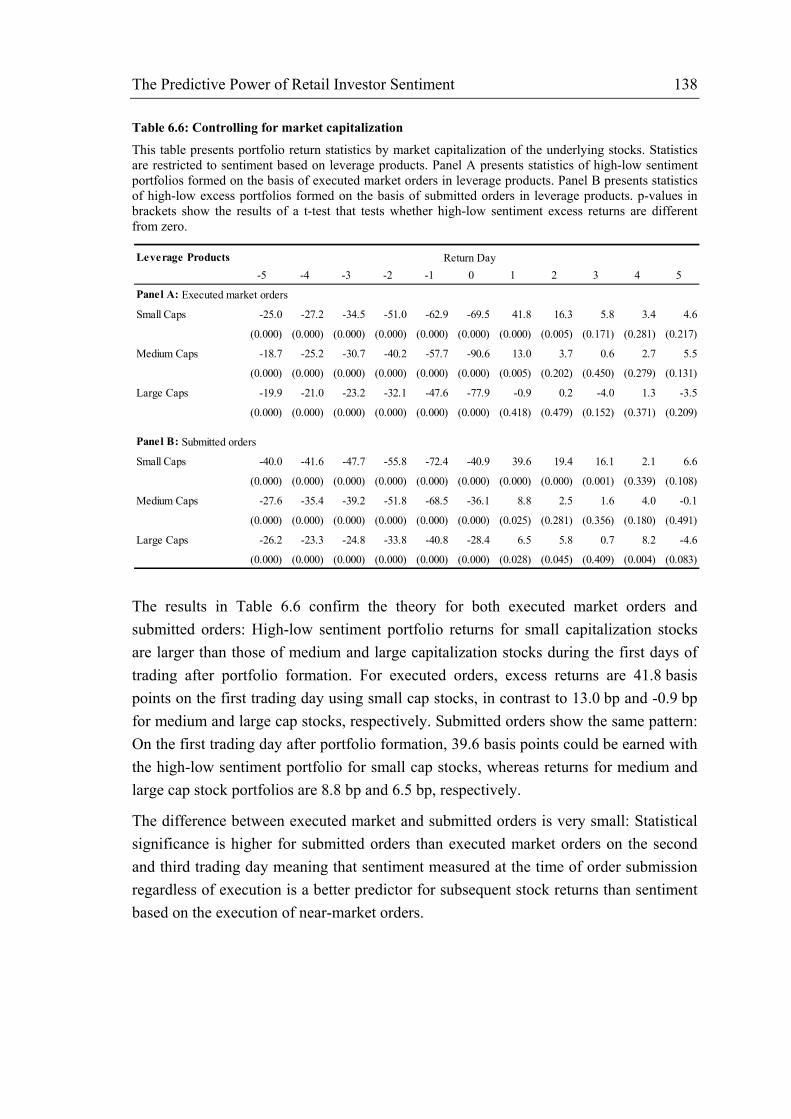
The Predictive Power of Retail Investor Sentiment 138
Table 6.6: Controlling for market capitalization
This table presents portfolio return statistics by market capitalization of the underlying stocks. Statistics are restricted to sentiment based on leverage products. Panel A presents statistics of high-low sentiment portfolios formed on the basis of executed market orders in leverage products. Panel B presents statistics of high-low excess portfolios formed on the basis of submitted orders in leverage products. p-values in brackets show the results of a t-test that tests whether high-low sentiment excess returns are different from zero.
The results in Table 6.6 confirm the theory for both executed market orders and submitted orders: High-low sentiment portfolio returns for small capitalization stocks are larger than those of medium and large capitalization stocks during the first days of trading after portfolio formation. For executed orders, excess returns are 41.8 basis points on the first trading day using small cap stocks, in contrast to 13.0 bp and -0.9 bp for medium and large cap stocks, respectively. Submitted orders show the same pattern: On the first trading day after portfolio formation, 39.6 basis points could be earned with the high-low sentiment portfolio for small cap stocks, whereas returns for medium and large cap stock portfolios are 8.8 bp and 6.5 bp, respectively.
The difference between executed market and submitted orders is very small: Statistical significance is higher for submitted orders than executed market orders on the second and third trading day meaning that sentiment measured at the time of order submission regardless of execution is a better predictor for subsequent stock returns than sentiment based on the execution of near-market orders.
Leverage Products-5 -4 -3 -2 -1 0 1 2 3 4 5
Panel A: Executed market orders
Small Caps -25.0 -27.2 -34.5 -51.0 -62.9 -69.5 41.8 16.3 5.8 3.4 4.6
(0.000) (0.000) (0.000) (0.000) (0.000) (0.000) (0.000) (0.005) (0.171) (0.281) (0.217)
Medium Caps -18.7 -25.2 -30.7 -40.2 -57.7 -90.6 13.0 3.7 0.6 2.7 5.5
(0.000) (0.000) (0.000) (0.000) (0.000) (0.000) (0.005) (0.202) (0.450) (0.279) (0.131)
Large Caps -19.9 -21.0 -23.2 -32.1 -47.6 -77.9 -0.9 0.2 -4.0 1.3 -3.5
(0.000) (0.000) (0.000) (0.000) (0.000) (0.000) (0.418) (0.479) (0.152) (0.371) (0.209)
Panel B: Submitted orders
Small Caps -40.0 -41.6 -47.7 -55.8 -72.4 -40.9 39.6 19.4 16.1 2.1 6.6
(0.000) (0.000) (0.000) (0.000) (0.000) (0.000) (0.000) (0.000) (0.001) (0.339) (0.108)
Medium Caps -27.6 -35.4 -39.2 -51.8 -68.5 -36.1 8.8 2.5 1.6 4.0 -0.1
(0.000) (0.000) (0.000) (0.000) (0.000) (0.000) (0.025) (0.281) (0.356) (0.180) (0.491)
Large Caps -26.2 -23.3 -24.8 -33.8 -40.8 -28.4 6.5 5.8 0.7 8.2 -4.6
(0.000) (0.000) (0.000) (0.000) (0.000) (0.000) (0.028) (0.045) (0.409) (0.004) (0.083)
Return Day
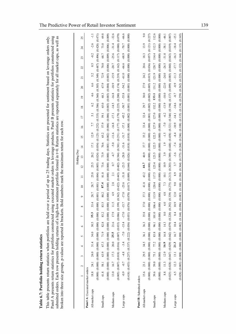
The Predictive Power of Retail Investor Sentiment 139
Tab
le 6
.7: P
ortf
olio
hol
ding
ret
urn
stat
istic
s
This
tabl
e pr
esen
ts re
turn
sta
tistic
s w
hen
portf
olio
s ar
e he
ld o
ver a
per
iod
of u
p to
25
tradi
ng d
ays.
Stat
istic
s ar
e pr
esen
ted
for s
entim
ent b
ased
on
leve
rage
ord
ers
only
. Pa
nel A
pre
sent
s re
turn
sta
tistic
s fo
r por
tfolio
s co
nstru
cted
usi
ng e
xecu
ted
mar
ket o
rder
s in
leve
rage
pro
duct
s. Pa
nel B
pre
sent
s st
atis
tics
for p
ortfo
lios
cons
truct
ed u
sing
su
bmitt
ed o
rder
s. Ea
ch ro
w p
rese
nts h
oldi
ng re
turn
s of a
hig
h-lo
w se
ntim
ent p
ortfo
lio fo
rmed
in t=
0. R
etur
n st
atis
tics a
re re
porte
d se
para
tely
for a
ll m
arke
t cap
s, as
wel
l as
brok
en in
to th
ree
size
gro
ups.
p-va
lues
are
repo
rted
in b
rack
ets.
Bol
d nu
mbe
rs m
ark
the
max
imum
retu
rn fo
r eac
h ro
w.
12
34
56
78
910
1112
1314
1516
1718
1920
2122
2324
25
Pane
l A: E
xecu
ted
mar
ket o
rder
s
All
mar
ket c
aps
18.8
24.1
24.0
31.4
34.0
30.5
35.3
33.4
28.7
28.7
25.8
25.5
20.2
17.1
12.9
7.7
5.1
6.2
4.6
6.6
5.2
0.5
-0.2
-2.6
-1.1
(0.0
00)
(0.0
00)
(0.0
00)
(0.0
00)
(0.0
00)
(0.0
00)
(0.0
00)
(0.0
00)
(0.0
01)
(0.0
01)
(0.0
04)
(0.0
05)
(0.0
24)
(0.0
54)
(0.1
25)
(0.2
52)
(0.3
35)
(0.3
06)
(0.3
60)
(0.3
05)
(0.3
49)
(0.4
87)
(0.4
96)
(0.4
28)
(0.4
71)
Smal
l cap
s41
.858
.163
.967
.371
.982
.883
.283
.580
.287
.481
.073
.673
.970
.665
.257
.959
.165
.068
.367
.972
.970
.068
.773
.069
.8
(0.0
00)
(0.0
00)
(0.0
00)
(0.0
00)
(0.0
00)
(0.0
00)
(0.0
00)
(0.0
00)
(0.0
00)
(0.0
00)
(0.0
00)
(0.0
00)
(0.0
00)
(0.0
01)
(0.0
02)
(0.0
06)
(0.0
06)
(0.0
03)
(0.0
03)
(0.0
04)
(0.0
03)
(0.0
06)
(0.0
09)
(0.0
06)
(0.0
09)
Med
ium
cap
s13
.016
.717
.320
.025
.521
.617
.911
.54.
92.
82.
10.
7-4
.7-5
.0-1
1.6
-16.
8-1
7.1
-14.
5-1
6.8
-18.
9-1
5.9
-20.
7-2
5.6
-31.
4-3
2.6
(0.0
05)
(0.0
07)
(0.0
18)
(0.0
16)
(0.0
07)
(0.0
33)
(0.0
86)
(0.1
99)
(0.3
62)
(0.4
22)
(0.4
43)
(0.4
82)
(0.3
84)
(0.3
81)
(0.2
51)
(0.1
77)
(0.1
79)
(0.2
25)
(0.2
00)
(0.1
74)
(0.2
19)
(0.1
62)
(0.1
17)
(0.0
80)
(0.0
79)
Larg
e ca
ps-0
.9-0
.7-4
.8-3
.4-7
.0-1
5.4
-17.
0-1
5.7
-17.
0-2
5.6
-31.
0-2
3.5
-28.
0-3
1.6
-31.
7-3
7.1
-45.
2-5
0.7
-55.
8-5
4.2
-61.
0-6
6.6
-68.
9-7
0.7
-66.
6
(0.4
18)
(0.4
53)
(0.2
57)
(0.3
37)
(0.2
22)
(0.0
56)
(0.0
51)
(0.0
76)
(0.0
70)
(0.0
17)
(0.0
09)
(0.0
44)
(0.0
26)
(0.0
18)
(0.0
18)
(0.0
08)
(0.0
02)
(0.0
01)
(0.0
01)
(0.0
01)
(0.0
00)
(0.0
00)
(0.0
00)
(0.0
00)
(0.0
00)
Pane
l B: S
ubm
itted
ord
ers
All
mar
ket c
aps
15.6
23.1
29.5
34.5
36.1
36.3
35.8
37.0
37.3
41.8
43.2
44.7
40.9
37.7
35.2
33.4
32.4
29.7
30.0
27.9
24.2
20.6
18.3
13.9
9.0
(0.0
00)
(0.0
00)
(0.0
00)
(0.0
00)
(0.0
00)
(0.0
00)
(0.0
00)
(0.0
00)
(0.0
00)
(0.0
00)
(0.0
00)
(0.0
00)
(0.0
00)
(0.0
00)
(0.0
00)
(0.0
00)
(0.0
01)
(0.0
02)
(0.0
02)
(0.0
05)
(0.0
15)
(0.0
36)
(0.0
57)
(0.1
21)
(0.2
27)
Smal
l cap
s39
.659
.075
.177
.283
.896
.110
1.0
106.
411
3.9
120.
411
7.5
125.
412
3.5
122.
512
2.5
127.
912
7.0
132.
213
3.1
131.
212
1.9
120.
711
4.4
112.
311
2.6
(0.0
00)
(0.0
00)
(0.0
00)
(0.0
00)
(0.0
00)
(0.0
00)
(0.0
00)
(0.0
00)
(0.0
00)
(0.0
00)
(0.0
00)
(0.0
00)
(0.0
00)
(0.0
00)
(0.0
00)
(0.0
00)
(0.0
00)
(0.0
00)
(0.0
00)
(0.0
00)
(0.0
00)
(0.0
00)
(0.0
00)
(0.0
00)
(0.0
00)
Med
ium
cap
s8.
811
.312
.916
.916
.814
.38.
06.
04.
87.
310
.110
.93.
91.
9-1
.5-7
.0-6
.2-1
3.9
-18.
0-2
2.0
-24.
0-2
6.5
-31.
0-3
8.1
-46.
1
(0.0
25)
(0.0
28)
(0.0
47)
(0.0
29)
(0.0
42)
(0.0
79)
(0.2
20)
(0.2
92)
(0.3
39)
(0.2
75)
(0.2
13)
(0.2
03)
(0.3
89)
(0.4
48)
(0.4
58)
(0.3
21)
(0.3
46)
(0.1
94)
(0.1
37)
(0.0
99)
(0.0
85)
(0.0
68)
(0.0
43)
(0.0
19)
(0.0
07)
Larg
e ca
ps6.
512
.313
.121
.316
.710
.48.
410
.912
.09.
08.
93.
7-3
.6-7
.4-8
.4-1
0.9
-14.
1-1
4.6
-8.7
-8.9
-11.
3-1
7.7
-16.
3-1
8.4
-15.
1
(0.0
28)
(0.0
03)
(0.0
08)
(0.0
00)
(0.0
08)
(0.0
82)
(0.1
44)
(0.0
96)
(0.0
83)
(0.1
68)
(0.1
84)
(0.3
64)
(0.3
75)
(0.2
68)
(0.2
46)
(0.1
88)
(0.1
35)
(0.1
34)
(0.2
59)
(0.2
62)
(0.2
25)
(0.1
22)
(0.1
44)
(0.1
15)
(0.1
65)
Hol
ding
Day

The Predictive Power of Retail Investor Sentiment 140
6.3.3. Portfolio Holding Returns
Having established that there are significant excess returns for a portfolio strategy that buys high sentiment stocks and sells low sentiment stocks, this section’s purpose is to analyze the portfolio holding returns of this strategy over a period of up to 25 trading days. The average cumulative returns of the high and the low sentiment portfolio as well as the resulting high-low sentiment portfolio are investigated in detail. Since the last section has shown that only sentiment based on leverage products has produced statistically significant results, this section focuses on sentiment based on leverage products only.
Table 6.7 reports portfolio holding return statistics for portfolios that are formed based on executed market orders (Panel A) as well as submitted orders (Panel B) over a period of up to 25 trading days.
The first lines of each Panel (all market caps) report average cumulative returns for the high-low sentiment portfolio. For executed market orders, the maximum return is reached on trading day 7 at 35.3 bp. For submitted orders, the maximum return is 44.7 bp on trading day 12. This difference suggests that the use of submitted orders might identify high potential stocks earlier than the use of executed market orders.
Figure 6.1 depicts the portfolio returns graphically. The high sentiment portfolio yields higher average returns than the low sentiment portfolio. The difference is the high-low sentiment portfolio with returns that are significantly different from zero. Table 6.7 provides p-values of the appropriate t-tests. Figure 6.1 also shows that the positive returns of the high-low sentiment portfolio are primarily caused by the negative returns of the low sentiment portfolio. Although the high sentiment portfolio yields significantly positive returns over the first five trading days, the cumulative returns become negative afterwards. The low sentiment portfolio, on the other hand, starts with negative returns and stays negative over the whole sample period of 25 trading days. Together, these two portfolios form the high-low sentiment portfolio and cause its returns to first increase and then revert to zero.
Figure 6.1 shows clearly that there is a pattern of reverting stock prices after initial periods of intense buying as predicted by theory and found by many empirical studies. However, a tendency of low-sentiment stock prices to revert cannot be found: Stock prices continue to decrease within the observation period of 25 trading days.

The Predictive Power of Retail Investor Sentiment 141
Figure 6.1: Portfolio holding returns
This figure presents average cumulative returns of portfolios that are held from the day of portfolio formation to up to 25 trading days. Returns of the low sentiment portfolio are represented by the red dotted line, those of the high sentiment portfolio by the green dashed line. The high-low sentiment portfolio excess returns are represented by the black solid line. Graph a) shows the results for sentiment on executed market orders in leverage products; graph b) shows the results for sentiment on submitted orders in leverage products.
The previous section has also shown that controlling for market capitalization is essential because portfolio excess returns depend on firm size. Table 6.7 also presents portfolio return statistics separately for different firm size groups: small caps, medium caps, and large caps. Again, the maximum return is marked by a bold number.
The results reveal that the significantly positive returns of the high-low sentiment portfolio are primarily driven by small capitalization stocks: For executed market orders, small cap portfolio returns are 87.4 bp in the maximum, whereas mid caps only yield 25.5 bp. The large caps portfolio does not yield any positive returns for the high-low sentiment strategy. Figure 6.2 depicts portfolio holding returns by firm size graphically.
-100-80-60-40-20
0204060
1 2 3 4 5 6 7 8 9 10 11 12 13 14 15 16 17 18 19 20 21 22 23 24 25Hol
ding
retu
rns i
n ba
sis p
oint
s
Holding days
a) Executed market orders
Low sentiment High sentiment High-low sentiment excess returns
-80-60-40-20
0204060
1 2 3 4 5 6 7 8 9 10 11 12 13 14 15 16 17 18 19 20 21 22 23 24 25Hol
ding
retu
rns i
n ba
sis p
oint
s
Holding days
b) Submitted orders
Low sentiment High sentiment High-low sentiment excess returns

The Predictive Power of Retail Investor Sentiment 142
Figure 6.2: Portfolio holding returns by market capitalization
This figure presents average cumulative returns of high-low sentiment portfolios that are held from the day of portfolio formation to up to 25 trading days. The black solid line shows results for the small cap portfolio, the green dashed line for the medium cap portfolio, and the red dotted line for the large cap portfolio. Graph a) shows the results for sentiment on executed market orders in leverage products; graph b) shows the results for sentiment on submitted orders in leverage products.
Figure 6.2 shows very convincingly that the strategy of buying high sentiment stocks and selling low sentiment stocks only works for small capitalization stocks. Returns for mid and large caps are very low or even negative. In addition, the maximum return point for this strategy on mid and large caps is reached within 4 or 5 trading days whereas the strategy for small caps reaches its maximum return on the 10th or 19th trading day (depending on the type of order used).
Figure 6.3 shows that – in comparison to the portfolios containing stocks of all sizes – the portfolios containing only high sentiment small firms show a longer tendency to yield significantly positive returns with a maximum on trading day 9, followed by decreasing holding returns before turning negative after trading day 21 (using sentiment
-90-60-30
0306090
120
1 2 3 4 5 6 7 8 9 10 11 12 13 14 15 16 17 18 19 20 21 22 23 24 25Hol
ding
retu
rns i
n ba
sis p
oint
s
Holding days
a) Executed market orders
Small caps Medium caps Large caps
-60-30
0306090
120150
1 2 3 4 5 6 7 8 9 10 11 12 13 14 15 16 17 18 19 20 21 22 23 24 25Hol
ding
retu
rns i
n ba
sis p
oint
s
Holding days
b) Submitted orders
Small caps Medium caps Large caps

The Predictive Power of Retail Investor Sentiment 143
based on submitted orders). Again, the negative sentiment portfolio does not seem to experience a reversion within the observation period of 25 trading days.
Figure 6.3: Portfolio holding returns for small caps
This figure presents average cumulative returns of portfolios consisting of small firms that are held from the day of portfolio formation to up to 25 trading days. Returns of the low sentiment portfolio are represented by the red dotted line, those of the high sentiment portfolio by the green dashed line. The high-low sentiment portfolio excess returns are represented by the black solid line. Graph a) shows the results for sentiment on executed market orders in leverage products; graph b) shows the results for sentiment on submitted orders in leverage products.
To sum up, a trading strategy consisting of buying small high sentiment stocks and selling small low sentiment stocks, with the sentiment based on all submitted orders in leverage products, generate economically and statistically significant excess returns of up to 133 basis points for a 19-day period.
6.4. Robustness Checks Several robustness checks are performed to assess the overall robustness of the results presented in the previous section.
-200
-150
-100
-50
0
50
100
1 2 3 4 5 6 7 8 9 10 11 12 13 14 15 16 17 18 19 20 21 22 23 24 25Hol
ding
retu
rns i
n ba
sis p
oint
s
Holding days
a) Executed market orders
Low sentiment High sentiment High-low sentiment excess returns
-200-150-100
-500
50100150
1 2 3 4 5 6 7 8 9 10 11 12 13 14 15 16 17 18 19 20 21 22 23 24 25Hol
ding
retu
rns i
n ba
sis p
oint
s
Holding days
b) Submitted orders
Low sentiment High sentiment High-low sentiment excess returns

The Predictive Power of Retail Investor Sentiment 144
Portfolio formation
Whether deciles, quintiles, or terciles should be used when constructing the high and low sentiment portfolios, cannot be unambiguously answered. Dorn, Huberman, and Sengmueller (2008) use terciles, Kaniel, Saar, and Titman (2008) use both deciles and quintiles, Pan and Poteshman (2006) and Barber, Odean, and Zhu (2009a) form quintiles, and Hvidkjaer (2008) uses deciles. There is no guidance in the former literature that would prefer any alternative.
However, the idea behind the portfolio formation technique is that only extreme sentiment should be captured and that portfolio excess returns are higher the more extreme the sentiment expression. Therefore, all portfolio calculations are performed with deciles as well as quintiles. The intuitive hypothesis that excess returns are larger when using more extreme sentiment can be confirmed. For example, excess returns for a high-low sentiment portfolio strategy involving submitted orders on leverage products are 12.97 basis points for quintiles compared to 15.65 basis points for deciles.
We can conclude that the choice of the portfolio quantile influences the magnitude of the portfolio excess returns. In choosing it, however, the absolute number of stocks in one portfolio must be considered resulting in a meaningful portfolio size.
Volume or trade based measure
Section 6.2.2 investigates the sentiment measure based on the number of executed orders instead of the volume based measure. As discussed in chapter 4, the number based sentiment and the volume based sentiment measures produce similar results with the difference that the former is robust to very large trades from a few individuals. After all, the number based measure is a better representation of the sentiment of retail investors as a whole.
A comparison of portfolio formation results using the volume based sentiment and the number based sentiment measure shows that the portfolio excess returns are not as large for the volume based measure as the excess returns for the number based measure, especially on the first day of the holding period. For example, instead of an excess return of 12.97 basis points (using quintiles of submitted orders on leverage products) for the number based measure, the value based measure yields an excess return of 10.85 basis points.
It can be shown that the volume based measure produces significantly positive excess returns but also that these excess returns are smaller in magnitude than the ones yielded when using the number based measure.

The Predictive Power of Retail Investor Sentiment 145
Minimum number of orders
The minimum number of orders restriction is crucial for meaningful sentiment values. Without it, extreme sentiment values could be constructed based on only one order resulting in a sentiment of plus one or minus one. As mentioned in section 6.2.2, additional tests using a minimum number of 5 or 10 orders per day and underlying show that the results are not changed significantly.
Portfolio formation period
Hvidkjaer (2008) uses portfolio formation periods of different lengths (from 1 to 24 months) and presents portfolio returns for different holding periods (from 1 to 36 months). Both Kaniel, Saar, and Titman (2008) and Barber, Odean, and Zhu (2009a) use a weekly formation period.
In the previous section, a portfolio formation period of one trading day is used in combination with portfolio holding periods of up to 30 trading days. In robustness checks, the formation period is increased to up to one week (5 trading days) to assess the influence on excess portfolio returns. These tests show that portfolio excess returns are highest when using a one-day portfolio formation period and are gradually lower when using a longer formation period of up to 5 trading days. For example, on the first trading day the excess returns of a strategy involving submitted orders on leverage products are 15.65 basis points using a formation period of one trading day, gradually declining to 11.66 basis points when using a formation period of five trading days.
In general, excess portfolio returns are highest when using the shortest formation period of one trading day. However, excess returns are still substantial and significant when using longer formation periods of up to five trading days.
Annual results
Another robustness check involves testing whether the results of section 6.3.3 are constant over time. In order to investigate this issue, average portfolio returns for the five different years in the sample are calculated and presented in Table 6.8. Only returns for strategies involving executed market orders and submitted orders for leverage products on small capitalization stocks are considered.

The Predictive Power of Retail Investor Sentiment 146
Table 6.8: Annual portfolio holding returns
This table presents portfolio holding returns for a high-low sentiment portfolio of small capitalization stocks using orders in leverage products for portfolio formation. Results are reported for each year of the sample period separately. Panel A shows results for executed market orders; Panel B shows results for submitted orders. p-values are reported in brackets.
The results indicate that in all five different annual periods excess returns are significantly positive, at least for the first days of the holding period. Of course there are differences in magnitude with the year 2008 being the period with the highest excess returns and the year 2007 the one with the lowest – considering the maximum returns are within the first 10 holding days.
Overall, these results confirm the robustness of the trading strategy involving the high minus low sentiment portfolio formation to the specific time period.
Year 1 2 3 4 5 6 7 8 9 10
Panel A: Executed market orders
High-low sentiment portfolio returns
2004 38.9 52.7 55.1 53.5 41.6 77.7 64.8 55.7 44.8 65.0
(0.027) (0.026) (0.040) (0.061) (0.131) (0.032) (0.075) (0.125) (0.182) (0.100)
2005 26.6 54.8 61.1 48.3 65.1 73.3 72.0 75.0 71.5 68.9
(0.012) (0.003) (0.003) (0.026) (0.010) (0.005) (0.015) (0.015) (0.024) (0.036)
2006 41.5 56.7 51.5 38.8 45.4 59.5 68.3 82.6 85.1 94.8
(0.003) (0.002) (0.007) (0.050) (0.039) (0.015) (0.013) (0.006) (0.007) (0.003)
2007 25.1 29.3 43.8 61.6 65.0 60.6 52.1 37.8 37.3 38.5
(0.008) (0.030) (0.009) (0.003) (0.004) (0.010) (0.030) (0.112) (0.126) (0.123)
2008 77.1 96.8 107.6 133.8 141.9 142.5 158.4 166.5 162.3 169.9
(0.000) (0.000) (0.000) (0.000) (0.000) (0.000) (0.000) (0.000) (0.001) (0.000)
Panel B: Submitted orders
High-low sentiment portfolio returns
2004 21.8 67.9 81.8 66.6 58.0 54.4 67.3 67.0 76.7 81.0
(0.055) (0.000) (0.000) (0.009) (0.030) (0.050) (0.028) (0.031) (0.023) (0.025)
2005 38.2 55.5 81.7 93.6 120.3 137.8 133.4 152.9 157.0 168.4
(0.000) (0.000) (0.000) (0.000) (0.000) (0.000) (0.000) (0.000) (0.000) (0.000)
2006 38.4 43.6 46.9 42.6 44.3 61.5 62.5 74.3 76.1 77.3
(0.000) (0.001) (0.001) (0.008) (0.016) (0.003) (0.003) (0.001) (0.002) (0.002)
2007 31.8 36.7 53.1 63.4 64.4 56.8 49.2 22.4 14.5 20.0
(0.000) (0.002) (0.000) (0.000) (0.001) (0.009) (0.032) (0.204) (0.303) (0.247)
2008 68.0 90.8 111.7 119.9 132.8 171.5 193.5 217.2 246.9 256.7
(0.000) (0.000) (0.000) (0.000) (0.000) (0.000) (0.000) (0.000) (0.000) (0.000)
Holding day

The Predictive Power of Retail Investor Sentiment 147
6.5. Conclusion In this chapter, sentiment measures for different stocks are being developed based on Euwax Sentiment measures for single underlyings. It is shown that a trading strategy based on these sentiment measures is able to generate abnormal returns.
Related studies provide a mixed picture of whether retail sentiment data can be used to predict returns. In most cases, this is clearly a shortcoming of the data set used. Data sets usually differ in the following ways: origin of the data, exact identification of trade direction, exact identification of retail trades, country of origin, and short-sale restrictions. The unique data set used in this chapter tries to avoid known problems by including only retail investor orders from different brokerages, the explicit trade direction, and the possibility of expressing negative sentiment through put options. In addition, order types, product types, and market capitalization of the underlying firms are distinguished. Furthermore, the data set used in this work is the first data set using submitted orders to create order imbalance measures.
The methodology applied in this chapter is especially useful for detecting differences between extreme high sentiment and extreme low sentiment measurements. A high sentiment portfolio is constructed using stocks with extreme positive sentiment readings, and a low sentiment portfolio is constructed consisting of stocks with extreme negative sentiment readings. The returns of a long-short strategy involving buying the high sentiment portfolio and selling the low sentiment portfolio indicate that high sentiment stocks perform better than low sentiment stocks, and that the trading strategy yields abnormal returns.
Several filters are used on the data to assess the influence of distinguishing between product and order type as well as using submitted or executed orders. In general, sentiment based on market orders in leverage products has predictive power for the next trading days’ returns whereas no such results can be found for sentiment based on limit orders and investment certificates. Furthermore, sentiment based on submitted orders shows the same predictive power, with even stronger returns on the first four trading days after portfolio formation.
Results remain statistically and economically significant even when controlling for market returns and momentum. However, controlling for market capitalization reveals that only small firm sentiment has significant predictive power whereas sentiment based on large firms does not produce significant results. This does not weaken the overall results. Calculating three separate portfolios for small, medium, and large firms rather controls for the SMB (small minus big) effect resulting in three high-low sentiment portfolios that are not influenced by this effect. Moreover, the results are in line with existing theory on noise trading and sentiment finding that small firm stocks are more likely to be influenced by retail investor trades.

Conclusion and Future Work 148
7 Conclusion and Future Work
This chapter concludes this work. Section 7.1 reviews the research questions from Chapter 1 and briefly summarizes the answers provided in the various chapters of this work. Section 7.2 points out the key contributions, and section 7.3 completes this chapter with an overview of open questions and avenues of future research.
7.1. Conclusion This section revisits the research questions as they are developed in the introduction of this work and briefly summarizes the answers given in the chapters following the introduction.
Research Question 1:
How can investor sentiment be measured and how are different sentiment indicators related?
Investor sentiment measures can be categorized according to the way they are created: Direct sentiment measures are surveys in which investors are asked directly about their attitude towards the economic situation or the stock market in particular. Indirect sentiment measures are usually created from financial variables and therefore measure sentiment only indirectly. Meta-measures are sentiment measures that are neither based on surveys nor pure financial data but involve meta-information about investor sentiment.
To investigate the differences between existing sentiment measures, two methodologies have been used: First, correlation of all sentiment indicators within a category as determined for the first part of the question is calculated to evaluate these against each other. In addition, correlation of all sentiment indicators between two categories is calculated to check whether they all rest on the same sources. Second, all sentiment indicators are compared to various contemporaneous market returns since sentiment measures and market returns should be correlated.
In general, most of the measures, regardless of whether they are indirect or direct, have a high pairwise correlation indicating that they indeed pick up the same sentiment signal. Furthermore, most of the sentiment indicators correlate well with market returns, with high-frequency indirect measures having the highest correlation and lower-frequency indirect measures a lower correlation with the market.

Conclusion and Future Work 149
To conclude, there are many different measures of investor sentiment in research and practice but their evaluation remains difficult. A high correlation among each other and with market returns is a good indication that they react to the same underlying factor but does not serve as a necessary or sufficient condition. Future research is needed to identify this factor which will make it easier to construct new measures and evaluate existing ones.
Research Question 2:
Can an index be created from retail order flow data to describe investor sentiment?
This research question is being answered by developing a retail investor sentiment index as a proof-of-concept using data that has not been used before for that purpose. The Euwax Sentiment Index is based on executed retail investor orders in leverage products on the DAX and includes only market orders.
The unique data set from Boerse Stuttgart has several advantages over previously used data sets: First, it consists of retail investor orders only, i.e. there is no need for a trade classification by trade size as it has to be done for other data sets. Second, orders can be exactly classified as buy and sell orders without the need to infer the trade direction using signing algorithms such as the one by Lee and Ready (1991). Third, the data set allows for a more symmetric expression of retail sentiment since retail investors have the opportunity to invest in puts to express negative sentiment. Fourth, in addition to executed orders, the data set comprises submitted orders which provide further insights into the dynamic relationship between order submission and execution.
The results can be summarized as follows: First, sentiment extracted from orders in leverage products has a higher correlation with market returns than sentiment from orders in investment products. Second, market orders better represent sentiment because changes in sentiment are captured exactly when the order decision is made by the investor. In contrast, limit orders are executed without the necessity of a simultaneous order submission. Therefore, sentiment extracted from executed limit orders may include orders that have been submitted much earlier and do not represent actual sentiment. As an alternative to executed market orders, sentiment may also be extracted from submitted orders to circumvent the problem of delayed order execution.
However, the regression results reveal that sentiment is negatively correlated to market returns regardless of whether submitted orders, executed limit orders or executed market orders are used to generate the sentiment measure. The results confirm that retail investors act as contrarians, and that this is not just because their limit order trades lead us to believe it as suggested by Linnainmaa (2009).

Conclusion and Future Work 150
The comparison with other existing sentiment measures shows that in the majority of cases there is a significant correlation between sentiment measures. However, the exact causality for this correlation cannot be determined. It is possible that different sentiment measures are driven by the same factors, but that these factors influence sentiment in different ways. For example, a large negative correlation between the Euwax Sentiment and the weekly German investor sentiment surveys can be documented. The negative correlation means that sentiment extracted from order flow data is contrary to that extracted from investor surveys. On the other hand, there are large positive correlations between Euwax Sentiment and other indirect measures of sentiment. It can be concluded that most of the sentiment measures are related but the unambiguous interpretation remains open and subject of future research.
Research Question 3:
Do retail investors herd?
The answer of this question needs an unambiguous definition of herding which does not exist in the literature. For the purpose of this study, the definition by Lakonishok, Shleifer, and Vishny (1992) is followed who define herding as “buying (selling) simultaneously the same stocks as others buy (sell)” but extend the definition to assets in general. Therefore, the order flow data from Boerse Stuttgart can be used to determine the level of herding for retail investors.
Herding as defined above has two dimensions: choice of time and choice of assets. The first dimension refers to retail investors (de-)investing in the market at the same time. This tendency is also called market-level herding. Market-level herding is analyzed by looking at aggregate retail investor order flow measures in securitized derivatives on the DAX. The second dimension of herding refers to retail investors choosing the same securities at the same time which is also called stock-level herding. Instead of the stocks themselves, securitized derivatives on those stocks are analyzed to detect stock-level herding.
On the market level, retail investors show a strong tendency of herding: More than 10% of all investors than expected by chance are on the same side of the market each day. This result holds across order types proving that this is not a result of automatic limit order execution. Furthermore, it is shown that optimistic herding, i.e. herding when most investors are optimistic about the market, is more prevalent in bear markets than in bull markets, and that pessimistic herding is more prevalent in bull than in bear markets. This finding supports the finding that retail investors act as contrarians. Moreover, herding is higher in bear markets than in bull markets, indicating that retail investors are collectively seeking investment opportunities in bear markets.
This finding is not a broker-specific phenomenon: The additional analysis shows that a substantial amount of herding is detected across all brokers and all types of brokers

Conclusion and Future Work 151
although there are differences between broker types: Analyzing the order flows of 22 different brokers in four distinct categories reveals that the level of herding is highest among public brokers with a rather conservative clientele and lowest among online brokers that neither give investment advice nor operate any branches.
On the stock level, the level of herding is similar to that found on the market level, and to those reported in other recent studies: Retail investors herd into and out of the same assets (underlying stocks) at the same time.
With respect to the theory, the empirical evidence supports the hypothesis that retail investors act in concert and that their trades are correlated. This is contrary to arguments made by efficient markets proponents who argue that trades by uninformed investors (noise traders) cancel each other out and therefore do not have the ability to influence asset prices. Therefore, the correlated behavior of retail investors in the stock market should be studied more closely. The development of a herding measure can be regarded as a first step towards this goal.
Research Question 4:
Does sentiment predict returns?
In recent years, several studies using some sort of order imbalance measures have tried to answer this question. However, the studies provide a mixed picture of whether retail sentiment data can be used to predict returns. In most cases, this is a shortcoming of the data set used. The data sets used by related work differ in many ways: There are differences concerning the source of the data, its frequency and period, regional focus, target group, and the construction of the imbalance measure.
In this work, a unique data set with executed and submitted retail investor orders on 244 underlying stocks is used to calculate sentiment measures for each stock. The relationship between sentiment measures and the corresponding returns is analyzed to evaluate whether sentiment positively predicts returns, i.e. high sentiment is followed by positive returns, and low sentiment is followed by negative returns.
This is done with a portfolio construction methodology: A high sentiment portfolio is constructed using stocks with extreme positive sentiment readings, and a low sentiment portfolio is constructed consisting of stocks with extreme negative sentiment readings. If high sentiment stocks perform better than low-sentiment stocks, a long-short trading strategy involving buying the high sentiment portfolio and selling the low sentiment portfolio should yield positive excess returns. This methodology is especially useful for detecting differences between extreme high sentiment and extreme low sentiment measurements. In addition, it provides a direct assessment of the economic significance, i.e. the absolute excess returns of the trading strategy.

Conclusion and Future Work 152
The results reveal that sentiment – measured by retail investor market orders in leverage products – indeed positively predicts stock returns. Submitted orders in leverage products have the highest predictive power but only for small firms: The analysis of the five year historical data set shows that holding the long-short portfolio for 10 consecutive days yields 120 basis points excess returns.
Overall, the results show that the average retail investor order flow does not represent “dumb money” as suggested by market folklore – at least not for EUWAX investors. The results shows that retail investors have a rather good feeling for market timing as well as for picking stocks that do well in the short term.
7.2. Summary of Contributions
Reconciliation of empirical findings
The growing body of empirical research on order flow and prices demands a more detailed analysis and a critical comparison of the related findings. Recent research shows that findings concerning correlated trading and return predictability may be different and even contradictory. The literature currently does not present a reconciliation of all relevant studies25. Section 2.4 in Chapter 2 aims to close this gap and presents a structured overview of recent findings and offers explanations for any differences found.
Extensive overview and comparison of investor sentiment measures
Many investor sentiment measures have been developed and are currently used in practice. There is a relatively large body of research covering single sentiment measures and especially their relation to returns and volatility. An overview of current sentiment measures and a correlation analysis, however, are missing26. Chapter 3 evaluates existing direct and indirect sentiment measures and presents correlation coefficients among them as well as correlation to contemporaneous market returns.
Construction of a new sentiment index
One of the main contributions of this work is the construction of a new sentiment index based on a unique data set using retail investor orders to the European Warrant Exchange in Chapter 4. Moreover, this work is among the first to use data on securitized derivatives27. These products are especially suited for the creation of a retail investor sentiment measure because retail investors have the possibility to express both positive and negative market sentiment with the purchase of a single product. 25 Barber, Hvidkjaer, Odean, and Zhu (2006) only present a reconciliation of their own work. 26 Brown and Cliff (2004) present an overview of sentiment measures, but do not include important German survey measures. 27 Schmitz, Glaser, and Weber (2007) use warrant data, a subset of the securitized derivatives data.

Conclusion and Future Work 153
Investigation of herding behavior of retail investors
Chapter 5 focuses on the herding behavior of retail investors using the same data set on retail investor orders to EUWAX. There are not many studies about retail investor herding28 as most of the related work is concerned with the herding of institutional investors. In addition, two types of herding are distinguished: market-level herding and stock-level herding whereas most other studies exclusively investigate stock-level herding while omitting the fact that investors may move into and out of the market at the same time.
Moreover, the herding analysis is broken down to a broker level and sheds light on the question whether customers of different brokerages also show a different herding behavior. The order flow data enriched with non-public broker IDs allows for a classification into four distinct broker types that is typical for the German brokerage landscape. There is currently no other research that investigates the retail investor herding behavior of different German brokers.
Analysis of submitted retail investor orders
Recent research29 on order imbalance measures argues that the use of executed retail investor orders may lead to wrong conclusions with respect to the contrarian behavior of retail investors. This work alleviates these concerns by using submitted orders instead of executed orders. This is the first study to use the order submission time for this purpose.
Development of a trading strategy
For evaluation purposes, a trading strategy is developed in Chapter 6 which consists of buying high sentiment stocks and selling low sentiment stocks resulting in a zero-cost portfolio that generates abnormal returns. While this methodology has also been used by other recent empirical studies30, it provides several new aspects regarding the use of different order types, the exact classification of buy and sell orders, the influence of market capitalization, and the use of submitted instead of executed orders. No other related work addresses all of these aspects and provides such a high degree of detail in its analysis.
28 Dorn, Huberman, and Sengmueller (2008) explicitly calculate an individual investor herding measure. 29 Linnainmaa (2009) argues that individual investors have been falsely classified as contrarian. 30 Jackson (2003), Pan and Poteshman (2006), Kaniel, Saar, and Titman (2008), Dorn, Huberman, and Sengmueller (2008), and Barber, Odean, and Zhu (2009a) use similar portfolio construction methodologies.

Conclusion and Future Work 154
7.3. Future Work While many issues have been addressed, there are still open questions which have arisen in the process of this work and which provide possible future research directions which are outlined briefly in this section.
Unified Investor Sentiment Theory
While this work focuses on the empirical investigation of retail investor sentiment, a unified theory of investor sentiment that brings together theory and empiricism is still missing. There have been some attempts to create a theory of investor sentiment but these do not explain all empirical findings.
In particular, a theory should incorporate short-term as well as long-term considerations since empirical research31 indicates that short-term effects differ from long-term effects. These different patterns still have to be explained by market microstructure theory.
Individual retail investor behavior
While this work focuses on the aggregate behavior of retail investors, a detailed investigation of individual investor behavior is needed to better understand the motivation of retail investors for trading. Although the data set used in this work presents valuable insights into retail investor behavior, its main drawback is the missing link to individual account data.
Future work on individual account data32 – collected from large banks or brokers – which allows to track executed or submitted orders to individual accounts should focus on the motivation of retail investors to submit orders in particular stocks.
Moreover, individual account data offers the opportunity to investigate whether individual investors profit from trading by actually examining the exact holding period and account settlement data. In addition, individual retail investor account data allows for the identification of high-performance investors who continuously make profitable trading decisions and low-performance investors who usually make unprofitable decisions. If the distinction between high- and low-performance investors is persistent, then future research should be conducted to analyze the reason for this performance difference.
Experimental evidence
One possibility to get more insights into the thinking and behavior of retail investors is to conduct field or laboratory experiments. These experiments should be targeted 31 Barber, Hvidkjaer, Odean, and Zhu (2006) empirically show that the same analysis conducted on the same data sets for a monthly frequency and a weekly frequency is able to result in opposite patterns. 32 Data sets including individual account data are used e.g. in Schmitz, Glaser, and Weber (2007), Dorn, Huberman, and Sengmueller (2008), and Barber, Odean, and Zhu (2009b).

Conclusion and Future Work 155
towards finding evidence about their individual motivation to trade assets and the timing of their trading decision.
Survey evidence
Some of the open research questions mentioned above could be addressed by conducting surveys among retail investors. Surveys offer the possibility to directly ask investors about their motivation to trade and about possible information sources they have used to come to their concrete trading decision.
Explanation of contrarian and herding behavior
The empirical evidence in this work shows that retail investors – at least EUWAX investors trading securitized derivatives – act as contrarians, i.e. they buy when the market declines and sell when the market rises. However, the reason why retail investors show a contrarian behavior remains opaque. Further research is needed to figure out why investors think that they could earn abnormal returns by following a contrarian strategy, and whether they actually succeed by doing so.
Closely related to the contrarian behavior, the exact reasons for the herding behavior of retail investors remain to be subject of future research. While much has been done to explain the herding behavior of institutional investors theoretically, retail investors have not received such a great deal of attention. The question is whether they are following each others’ trades (which is unlikely since their trades are generally not public) or whether they are following the same signals.
Moreover, if following the same signals lead retail investors to act as contrarians, then both research questions are closely related and must be considered together.

Appendices ix
Appendices
A Appendix to Chapter 4 Table A.1: Summary statistics on executed order volume
This table reports summary statistics about the volume of executed orders by derivative product group (warrants, knock-outs, and investment certificates). Panel A groups the orders by option type and trade direction, Panel B by order type, and Panel C by underlying type. The percentages in brackets provide information about the relative use of the different order classes within each product group.
Call Buy 15,900 (37.9%) 24,226 (35.6%) 50,494 (49.7%) 90,620 (42.8%)
Sell 15,995 (38.1%) 25,417 (37.3%) 48,424 (47.6%) 89,836 (42.4%)
Put Buy 5,017 (12.0%) 8,923 (13.1%) 1,325 (1.3%) 15,265 (7.2%)
Sell 5,019 (12.0%) 9,487 (13.9%) 1,456 (1.4%) 15,962 (7.5%)
41,931 68,053 101,699 211,683
Panel B: Executed order volume (in million €) by order type
24,619 (58.7%) 42,758 (62.8%) 79,733 (78.4%) 147,110 (69.5%)
14,989 (35.7%) 17,330 (25.5%) 19,696 (19.4%) 52,015 (24.6%)
2,323 (5.5%) 7,965 (11.7%) 2,270 (2.2%) 12,558 (5.9%)
41,931 68,053 101,699 211,683
Panel C: Executed order volume (in million €) by underlying type
20,407 (48.7%) 10,486 (15.4%) 41,111 (40.4%) 72,004 (34.0%)
17,152 (40.9%) 48,002 (70.5%) 52,629 (51.8%) 117,784 (55.6%)
165 (0.4%) 758 (1.1%) 1,421 (1.4%) 2,344 (1.1%)
2,138 (5.1%) 2,062 (3.0%) 106 (0.1%) 4,306 (2.0%)
2,041 (4.9%) 2,062 (3.0%) 5,717 (5.6%) 9,820 (4.6%)
Other 28 (0.1%) 4,683 (6.9%) 714 (0.7%) 5,424 (2.6%)
41,931 68,053 101,699 211,683Total
Stop Orders
Total
Warrants Knock-outs
Stocks
Indices
Fixed Income
Currencies
Commodities
Investment certificates Total
Warrants Knock-outs Investment certificates Total
Total
Total
Market Orders
Limit Orders
Panel A: Executed order volume (in million €) by option type
Warrants Knock-outs Investment certificates

Appendices x
Table A.2: Summary statistics on submitted orders
This table reports summary statistics on the number of submitted orders by derivative product group (warrants, knock-outs, and investment certificates). Panel A groups the orders by option type and trade direction, Panel B by order type, and Panel C by underlying type. Panel D provides information about the execution status of submitted orders, i.e. whether they were filled or not. The percentages in brackets provide information about the relative use of the different order classes within each product group.
Call Buy 5,956,311 (41.2%) 4,841,590 (32.3%) 3,569,829 (50.0%) 14,367,730 (39.3%)
Sell 4,881,688 (33.7%) 5,011,605 (33.5%) 3,408,494 (47.8%) 13,301,787 (36.4%)
Put Buy 2,093,047 (14.5%) 2,481,306 (16.6%) 83,961 (1.2%) 4,658,314 (12.7%)
Sell 1,538,033 (10.6%) 2,643,003 (17.6%) 72,617 (1.0%) 4,253,653 (11.6%)
14,469,079 14,977,504 7,134,901 36,581,484
Panel B: Submitted orders by order type
5,814,127 (40.2%) 6,610,997 (44.1%) 4,930,479 (69.1%) 17,355,603 (47.4%)
7,802,032 (53.9%) 5,229,371 (34.9%) 1,811,306 (25.4%) 14,842,709 (40.6%)
852,920 (5.9%) 3,137,136 (20.9%) 393,116 (5.5%) 4,383,172 (12.0%)
14,469,079 14,977,504 7,134,901 36,581,484
Panel C: Submitted orders by underlying type
8,186,319 (56.6%) 3,228,694 (21.6%) 2,983,092 (41.8%) 14,398,105 (39.4%)
4,960,704 (34.3%) 8,813,129 (58.8%) 3,352,323 (47.0%) 17,126,156 (46.8%)
76,339 (0.5%) 247,922 (1.7%) 97,658 (1.4%) 421,919 (1.2%)
626,141 (4.3%) 696,693 (4.7%) 12,749 (0.2%) 1,335,583 (3.7%)
611,709 (4.2%) 1,604,189 (10.7%) 618,449 (8.7%) 2,834,347 (7.7%)
Other 7,867 (0.1%) 386,877 (2.6%) 70,630 (1.0%) 465,374 (1.3%)
14,469,079 14,977,504 7,134,901 36,581,484
Panel D: Submitted orders by execution status
8,177,580 (56.5%) 11,328,863 (75.6%) 5,985,030 (83.9%) 25,491,473 (69.7%)
6,291,499 (43.5%) 3,648,641 (24.4%) 1,149,871 (16.1%) 11,090,011 (30.3%)
14,469,079 14,977,504 7,134,901 36,581,484Total
Warrants Knock-outs Investment certificates Total
filled
not filled
Total
Stop Orders
Total
Warrants Knock-outs
Stocks
Indices
Fixed Income
Currencies
Commodities
Investment certificates Total
Warrants Knock-outs Investment certificates Total
Total
Total
Market Orders
Limit Orders
Panel A: Submitted orders by option type
Warrants Knock-outs Investment certificates

Bibliography xi
Bibliography
Andrade, S., Chang, C., Seasholes, M. S. (2008): Trading imbalances, predictable reversals, and cross-stock price pressure. Journal of Financial Economics, 88(2), 406-423.
Antweiler, W., Frank, M. Z. (2004): Is All That Talk Just Noise? The Information Content of Internet Stock Message Boards. The Journal of Finance, 59(3), 1259-1294.
Baker, M., Stein, J.C. (2004): Market liquidity as a sentiment indicator. Journal of Financial Markets, 7(3), 271-299.
Baker, M., Wurgler, J. (2006): Investor Sentiment and the Cross-Section of Stock Returns. The Journal of Finance, 61(4), 1645-1680.
Baker, M., Wurgler, J. (2007): Investor Sentiment and the Stock Market. The Journal of Economic Perspectives, 21(2), 129-151.
Bandopadhyaya, A., Jones, A. L. (2006): Measuring Investor Sentiment in Equity Markets. Journal of Asset Management, 7(3), 208-215.
Bandopadhyaya, A., Jones, A. L. (2008): Measures Of Investor Sentiment: A Comparative Analysis Put-Call Ratio Vs. Volatility Index. Journal of Business & Economics Research, 6(8), 27-34.
Barber, B. M., Hvidkjaer, S., Odean, T., Zhu, N. (2006): A Comparison of the Results in Barber, Odean, and Zhu (2006) and Hvidkjaer (2006). Working Paper, University of California, Davis.
Barber, B. M., Lee, Y., Liu, Y., Odean, T. (2005): Do Day Traders Make Money? Working Paper, University of California, Davis.
Barber, B. M., Lee, Y., Liu, Y., Odean, T. (2009): Just How Much Do Individual Investors Lose by Trading? Review of Financial Studies, 22(2), 609-632.
Barber, B. M., Odean, T., Zhu, N. (2009a): Do Retail Trades Move Markets? Review of Financial Studies, 22(1), 151-186.
Barber, B. M., Odean, T., Zhu, N. (2009b): Systematic noise. Journal of Financial Markets, 12(4), 547-569.
Barberis, N., Shleifer, A., Vishny , R. (1998): A model of investor sentiment. Journal of Financial Economics, 49(3), 307-343.
Beaumont, R., van Daele, M., Frijns, B., Lehnert, T. (2005): On Individual and Institutional Noise Trading, Working Paper, Maastricht University.
Berkman, H., Koch, P.D. (2008): Noise trading and the price formation process, Journal of Empirical Finance, 15(2), 232–250.
Black, F. (1986): Noise. The Journal of Finance, 41(3), 529-543.
Black, F., Scholes, M. (1973): The Pricing of Options and Corporate Liabilities, Journal of Political Economy, 81, 637–654.

Bibliography xii
Boehmer, E., Wu, J. (2008): Order Flow and Prices, AFA 2007 Chicago Meetings Paper.
Brown, G. W. (1999): Volatility, Sentiment, and Noise Traders. Financial Analysts Journal, 55(2), 82-90.
Brown, G. W., Cliff, M. T. (2004): Investor sentiment and the near-term stock market. Journal of Empirical Finance, 11(1), 1-27.
Brown, G. W., Cliff, M. T. (2005): Investor Sentiment and Asset Valuation. Journal of Business, 78(2), 405-440.
Burghardt, M. (2007): Investment Decisions and Behavior: Indicators for Investor Confidence. Proceedings of the Conference on Group Decision and Negotiation (Montreal, Canada) (Kersten, G. E.; Rios, J.; Chen, E., eds.).Volume I, 274–276.
Burghardt, M., Riordan, R. (2009): Know the Flow: Sentiment Extraction from Retail Order Flow Data. Proceedings of the FinanceCom 2008, Lecture Notes in Business Information Processing, 23 (D. Kundisch et al., ed.). Springer-Verlag. 31–46.
Campbell, J. Y., Kyle, A. S. (1993): Smart Money, Noise Trading and Stock Price Behaviour. The Review of Economic Studies, 60(1), 1-34.
Carhart, M. M. (1997): On Persistence in Mutual Fund Performance, The Journal of Finance, 52(1), 57-82.
Charoenrook, A. (2003): Does Sentiment Matter? Working Paper, Vanderbilt University.
Chordia, T., Roll, R., Subrahmanyam, A. (2002): Order imbalance, liquidity, and market returns. Journal of Financial Economics, 65(1), 111-130.
Chordia, T., Roll, R., Subrahmanyam, A. (2005): Evidence on the speed of convergence to market efficiency, Journal of Financial Economics, 76(2), 271-292.
Chordia, T., Subrahmanyam, A. (2004): Order imbalance and individual stock returns: Theory and evidence. Journal of Financial Economics, 72(3), 485–518.
Ciccone, S. (2003): Does Analyst Optimism About Future Earnings Distort Stock Prices? The Journal of Behavioral Finance, 4(2), 59-64.
Clarke, R. G., Statman, M. (1998): Bullish or Bearish? Financial Analysts Journal, 54(3), 63-72.
Coval, J. D., Hirshleifer, D. A., Shumway, T. (2005): Can Individual Investors Beat the Market? HBS Finance Working Paper No. 04-025, Harvard Business School.
Daniel, K., Hirshleifer, D., Subrahmanyam, A. (1998): Investor Psychology and Security Market Under- and Overreaction. The Journal of Finance, 53(6), 1839-1885.
Das, S. R., Chen, M. Y. (2007): Yahoo! for Amazon: Sentiment Extraction from Small Talk on the Web, Management Science, 53(9), 1375-1388.
Das, S., Martínez-Jerez, A., Tufano, P. (2005): eInformation: A Clinical Study of Investor Discussion and Sentiment. Financial Management, 34(3), 103-137.
De Bondt, W. F. M. (1998): A portrait of the individual investor. European Economic Review, 42(3-5), 831-844.

Bibliography xiii
De Bondt, W. F. M., Thaler, R. (1985): Does the Stock Market Overreact? The Journal of Finance, 40(3), 793-805.
De Long, J. B., Shleifer, A., Summers, L., Waldmann, R. (1990): Noise Trader Risk in Financial Markets. Journal of Political Economy, 98(4), 703-738.
Dorn, D., Huberman, G. (2005): Talk and Action: What Individual Investors Say and What They Do. Review of Finance, 9(4), 437-481.
Dorn, D., Huberman, G., Sengmueller, P. (2008): Correlated Trading and Returns. The Journal of Finance, 63(2), 885-920.
Edwards, W. (1968): Conservatism in human information processing. In B. Kleinmuntz (Ed.), Formal representation of human judgment. Wiley, New York.
Fabozzi, F. J., Francis, J. C. (1977): Stability Tests for Alphas and Betas over Bull and Bear Market Conditions. The Journal of Finance, 32(4), 1093-99.
Fama, E. F. (1965): The Behavior of Stock-Market Prices, The Journal of Business, 38(1), 34-105.
Fama, E. F. (1970): Efficient Capital Markets: A Review of Theory and Empirical Work. The Journal of Finance, 25(2), 383-417.
Fama, E. F. (1998): Market efficiency, long-term returns, and behavioral finance. Journal of Financial Economics, 49, 283-306.
Fama, E.F., Fisher, L., Jensen, M.C., Roll, R. (1969): The Adjustment of Stock Prices to New Information, International Economic Review, 10(1), 1 -21.
Fama, E.F., French, K. (1992): The cross-section of expected stock returns. The Journal of Finance, 47(2), 427-465.
Fama, E.F., French, K. (1993): Common risk factors in the returns on bonds and stocks. Journal of Financial Economics, 33(1), 3-56.
Fisher, K. L., Statman, M. (2000): Investor Sentiment and Stock Returns. Financial Analysts Journal, 56(2), 16-23.
Fisher, K. L., Statman, M. (2003): Consumer Confidence and Stock Returns. The Journal of Portfolio Management, 30(1), 115-127.
Frazzini, A., Lamont, O. A. (2008): Dumb Money: Mutual fund flows and the cross-section of stock returns. Journal of Financial Economics, 88(2), 299-322.
Friedman, M. (1953): The case for flexible exchange rates. Essays in Positive Economics. Chicago: University of Chicago Press.
Griffin, J. M., Harris, J. H., Topaloglu, S. (2003): The Dynamics of Institutional and Individual Trading. The Journal of Finance, 58(6), 2285-2320.
Grinblatt, M., Titman, S., Wermers, R. (1995): Momentum Investment Strategies, Portfolio Performance, and Herding – A Study of Mutual Fund Behavior. The American Economic Review, 85(5), 1088-1105.
Grossman, S. J., Stiglitz, J. E. (1980): On the Impossibility of Informationally Efficient Markets. The American Economic Review, 70(3), 393-408.
Groves, R. M. (1989): Survey Errors and Survey Costs. Wiley, New York.

Bibliography xiv
Han, B. (2008): Investor Sentiment and Option Prices. Review of Financial Studies, 21(1), 387-414.
Honcoop, D., Lehnert, T. (2007): Can Sentiment be predicted to have Cross-Sectional Effects? Working Paper, Maastricht University.
Hong, H., Stein, J. C. (1999): A Unified Theory of Underreaction, Momentum Trading, and Overreaction in Asset Markets. The Journal of Finance, 54(6), 2143-2184.
Hull, J. C. (2006): Options, futures, and other derivatives. 6th edition. Prentice Hall, Upper Saddle River, New Jersey.
Hvidkjaer, S. (2008): Small Trades and the Cross-Section of Stock Returns. Review of Financial Studies, 21(3), 1123-1151.
Jackson, A. (2003): The Aggregate Behaviour of Individual Investors. Working paper, London Business School.
Jayaraman, N., Frye, M. B., Sabherwal, S. (2001): Informed Trading around Merger Announcements: An Empirical Test Using Transaction Volume and Open Interest in Options Market. The Financial Review, 36, 45–74.
Jegadeesh, N, Titman, S. (1993): Profitability of Momentum Strategies: An Evaluation of Alternative Explanations. The Journal of Finance, 56(2), 699-720.
Kahneman, D., Tversky, A. (1979): Prospect Theory: An Analysis of Decision under Risk. Econometrica, 47(2), 263-291.
Kaniel, R., Saar, G., Titman, S. (2008): Individual Investor Trading and Stock Returns. The Journal of Finance, 63(1), 273-310.
Kraus, A., Stoll, H. R. (1972): Parallel Trading by Institutional Investors. The Journal of Financial and Quantitative Analysis, 7(5), 2107-2138.
Kumar, A., Lee, C. M. C. (2006): Retail Investor Sentiment and Return Comovements. The Journal of Finance, 61(5), 2451–2486.
Kurov, A. (2008): Investor Sentiment, Trading Behavior and Informational Efficiency in Index Futures Markets. The Financial Review, 43, 107-127.
Kyle, A. S. (1985): Continuous Auctions and Insider Trading. Econometrica, 53(6), 1315-1336.
Lakonishok, J., Shleifer, A., Vishny, R. W. (1992): The impact of institutional trading on stock prices. Journal of Financial Economics, 32(1), 23-43.
Lee, C. M. C., Radhakrishna, B. (2000): Inferring Investor Behavior: Evidence from TORQ, Journal of Financial Markets, 3(2), 83-111.
Lee, C. M. C., Ready, M. J. (1991): Inferring Trade Direction from Intraday Data. The Journal of Finance, 46(2), 733-46.
Lee, C. M. C., Shleifer, A., Thaler, R. H. (1991): Investor Sentiment and the Closed-End Fund Puzzle. The Journal of Finance, 46(1), 75-109.
Lee, W. Y., Jiang, C. X., Indro, D. C. (2002): Stock market volatility, excess returns, and the role of investor sentiment. Journal of Banking & Finance, 26, 2277-2299.
Lee, Y., Liu, Y., Roll, R., Subrahmanyam, A. (2004): Order Imbalances and Market Efficiency: Evidence from the Taiwan Stock Exchange. The Journal of Financial and Quantitative Analysis, 39(2), 327-341.

Bibliography xv
Lemmon, M., Portniaguina, E. (2006): Consumer Confidence and Asset Prices: Some Empirical Evidence. Review of Financial Studies, 19(4), 1499-1529.
Linnainmaa, J. (2009): Do Limit Orders Alter Inferences about Investor Performance and Behavior? The Journal of Finance, forthcoming.
Lo, A. W., ed. (1997): Market Efficiency: Stock Market Behaviour in Theory and Practice. Volumes I and II. Cheltenham, UK: Edward Elgar Publishing Company.
Martikainen, T., Puttonen, V. (1996): Call-put signal predict Finnish stock returns. Applied Economics Letters, 3(10), 645–648.
McHattie, A. (2002): Covered Warrants – New opportunities in an exciting new market. Harriman House Publishers, Petersfield, Great Britain.
Milgrom, P., Stokey, N. (1982): Information, Trade and Common Knowledge. Journal of Economic Theory, 26(1), 17-27.
Odean, T. (1998): Are Investors Reluctant to Realize Their Losses? The Journal of Finance, 53(5), 1775-1798.
Odean, T. (1999): Do Investors Trade Too Much? The American Economic Review, 89(5), 1279-1298.
Oehler, A. (1998): Do mutual funds specializing in German stocks herd? Finanzmarkt und Portfolio Management, 12(4), 452-465.
Otoo, M. W. (1999): Consumer Sentiment and the Stock Market. FEDS Working Paper No. 99-60.
Pan, J., Poteshman, A. M. (2006): The Information in Option Volume for Future Stock Prices. Review of Financial Studies, 19(3), 871-908.
Qiu, L. X., Welch, I. (2006): Investor Sentiment Measures. Working Paper, Brown University.
Ross, S. A. (2002): Neoclassical Finance, Alternative Finance and the Closed End Fund Puzzle. European Financial Management, 8(2), 129-137.
Ross, S. A., Westerfield, R. W., Jaffe, J. (2001): Corporate Finance. 6th Edition, McGraw-Hill.
Rozeff, M. S., Kinney, W. R. (1967): Capital market seasonality: The case of stock returns. Journal of Financial Economics, 3(4), 379-402.
Schmeling, M. (2007): Institutional and individual sentiment: Smart money and noise trader risk? International Journal of Forecasting, 23(1), 127-145.
Schmitz, P., Glaser, M., Weber, M. (2007): Individual Investor Sentiment and Stock Returns - What Do We Learn from Warrant Traders? Working Paper, Universität Mannheim.
Sharpe, W. F., Alexander, G. J. (1990): Investments. Prentice Hall, Englewood Cliffs, NJ.
Shefrin, H., Statman, M. (1985): The Disposition to Sell Winners Too Early and Ride Losers Too Long: Theory and Evidence. The Journal of Finance, 40(3), 777-790.
Shiller, R. J. (1984): Stock Prices and Social Dynamics. Brookings Papers on Economic Activity, 457-98.

Bibliography xvi
Shiller, R. J. (2000): Measuring Bubble Expectations and Investor Confidence. The Journal of Psychology and Financial Markets, 1(1), 49-60.
Shleifer, A. (2000): Inefficient Markets – An Introduction to Behavioral Finance. Clarendon Lectures in Economics. Oxford University Press. Oxford.
Shleifer, A., Summers, L. H. (1990): The Noise Trader Approach to Finance. The Journal of Economic Perspectives, 4(2), 19-33.
Shleifer, A., Vishny, R. W. (1997): The Limits of Arbitrage. The Journal of Finance, 52(1), 35-55.
Sias, R.W. (2004): Institutional Herding. Review of Financial Studies, 17(1), 165-206.
Simon, D. P., Wiggins, R. A. (2001): S&P Futures Returns and Contrary Sentiment Indicators. The Journal of Future Markets, 21(5), 447-462.
Solt, M. E., Statman, M. (1988): How Useful Is the Sentiment Index? Financial Analysts Journal, 44(5), 45-55.
Subrahmanyam, A. (2005): Distinguishing Between Rationales for Short-Horizon Predictability of Stock Returns. The Financial Review, 40, 11-35.
Subrahmanyam, A. (2007): Behavioural Finance: A Review and Synthesis. European Financial Management, 14(1), 12-29.
Subrahmanyam, A. (2008): Lagged order flows and returns: A longer-term perspective. The Quarterly Review of Economics and Finance, 48, 623-640.
Tetlock, P. C. (2007): Giving Content to Investor Sentiment: The Role of Media in the Stock Market. The Journal of Finance, 62(3), 1139-1168.
Tversky, A. and Kahneman, D. (1974): Judgment under Uncertainty: Heuristics and Biases. Science, 185(4157), 1124-1131.
Wang, Y., Keswani, A. Taylor, S. J. (2006): The relationships between sentiment, returns and volatility. International Journal of Forecasting, 22(1), 109-123.
Whaley, R. E. (2000): The investor fear gauge. Journal of Portfolio Management, 26(3), 1-6.
Zwergel, B., Klein, C. (2006): On the Predictive Power of Sentiment - Why Institutional Investors are Worth Their Pay. Working Paper, Universität Augsburg.