retracted: pricing currency options based on fuzzy techniques

Available online at www.sciencedirect.com

www.elsevier.com/locate/ejor

European Journal of Operational Research 193 (2009) 530–540

O.R. Applications

Pricing currency options based on fuzzy techniques

Fan-Yong Liu *

School of Finance and Economics, Hangzhou Dianzi University, Hangzhou, Zhejiang 310018, PR China

Received 26 August 2006; accepted 29 October 2007Available online 22 November 2007
D
Abstract

Owing to the fluctuation of financial markets from time to time, some financial variables can always be observed with perturbationsand be expected in the imprecise sense. Therefore, this paper starts from the fuzzy environments of currency options markets, introducesfuzzy techniques, and gives a fuzzy currency options pricing model. By turning exchange rate, interest rates and volatility into triangularfuzzy numbers, the currency option price will turn into a fuzzy number. This makes the financial investors who can pick any currencyoption price with an acceptable belief degree for their later use. In order to obtain the belief degree, an optimization procedure has beenapplied. An empirical study is performed based on daily foreign exchange market data. The empirical study results indicate that the fuzzycurrency options pricing method is a useful tool for modeling the imprecise problem in the real world.� 2007 Elsevier B.V. All rights reserved.

Keywords: Finance; Pricing; Fuzzy sets; Currency options CTE
1. Introduction
Since the closed-form solution of the European currency options pricing model was derived by Garman and Kohlhagen(1983) based on Black and Scholes (1973), many methodologies for the currency options pricing have been proposed byusing the modification of Garman–Kohlhagen (G–K) model, such as Amin and Jarrow (1991), Heston (1993), Bates(1996), Ekvall et al. (1997), Lim et al. (1998), Rosenberg (1998), Sarwar and Krehbiel (2000), Bollen and Rasiel (2003).

The input variables of the G–K model are usually regarded as the precise real numbers. However, in the real world, thesevariables cannot always be expected in a precise sense. For instance, the spot exchange rates fluctuate from time to timeaccording to the financial market effects and may occur imprecisely. It is more suitable and realistic to price currencyoptions under fuzzy environments because these variables are only available imprecise data or data related in a vagueway. Practically, many financial investors are concerned with the currency options price range, i.e. the confidence interval.The prices of currency options often oscillate within this confidence interval. The fuzzy sets theory proposed by Zadeh(1965) may be a useful tool for modeling this kind of imprecise problem. The book of collected papers edited by Ribeiroet al. (1999) gave the applications of using fuzzy sets theory to the discipline called financial engineering.

Next the motivation of this study is provided by explaining why it is need to take into account the fuzzy variables in theG–K model, such as the fuzzy exchange rate, the fuzzy domestic interest rate, the fuzzy foreign interest rate, and the fuzzyvolatility.

In the constant interest rates approach, when the financial investor tries to price a currency option, the interest rates,either domestic or foreign, are assumed as constant. However, the interest rates may have the different values in the dif-ferent commercial banks and financial institutions. Therefore, the choice of a reasonable interest rate may cause a dilemma.

RETRA

0377-2217/$ - see front matter � 2007 Elsevier B.V. All rights reserved.

doi:10.1016/j.ejor.2007.10.059

* Tel.: +86 136 16550891; fax: +86 571 86919196.E-mail address: [email protected]

mailto:[email protected]

F.-Y. Liu / European Journal of Operational Research 193 (2009) 530–540 531

But one thing can be sure is that the different interest rates may be around a fixed value within a short period of time. Forinstance, the interest rate may be around 5%, in this case, the interest rate may be regarded as a fuzzy number 5% when thefinancial investor tries to price a currency option using the G–K model.

On the other hand, there are two approaches used to obtain the volatilities in order to apply the G–K model, the so-calledhistorical volatility approach and implied volatility approach. Therefore, the choice of a reasonable volatility approach mayalso cause a dilemma. The other reason is that the international financial market fluctuates from time to time. It is a littleunreasonable to pick a fixed volatility to price an option at this time and then use this option price for the later use, since thelater volatility has already changed. In this case, it is natural to regard the volatility as an imprecise (fuzzy) data.

The usual approach for currency option pricing is to pick fixed input data to price an option by applying the G–Kmodel. However, this currency option price will be used for the further decision-making by a financial investor within ashort period of time. The problem is that the input data will be changed within this short period of time because the inter-national financial market fluctuates very irregular. Therefore, it is a little unreasonable to pick fixed input data to price acurrency option at this time and then use this price for later use, since the later these input data has already changed. There-fore, it is also natural to assume these input data as fuzzy numbers.

Although it has been described that how the four fuzzy input variables occur in the real world, some of four variablescan still be taken as the real (crisp) numbers if the financial investor can make sure that those variables occur in a crispsense. In this case, the methodology proposed in this paper is still applicable since the real numbers are the special caseof the fuzzy numbers. Now, under the considerations of the four fuzzy input variables, the currency option price will turninto a fuzzy number. This fuzzy number is in fact a function defined on R into [0,1], and denoted by membership functionl~a : X ! ½0; 1�. Given any value c, the function value l~aðcÞ will be interpreted as the belief degree of closeness to value a. Itmeans that the closer the value c to a is, the higher the belief degree is. Therefore, the financial investors can pick any valuethat is around a with an acceptable belief degree as the currency option price for their later use. In order to obtain the beliefdegree of any a given option price, an optimization problem will be given. An efficient computational procedure (Wu, 2005)is applied in this paper to solve this optimization problem.

The structure of this paper is as follows. In next Section, the notions and arithmetic of fuzzy numbers and the member-ship function of triangular fuzzy number are described. In Section 3, the fuzzy currency options pricing model is proposedand the computational procedure is introduced in order to obtain the belief degrees of any given option prices. In Section 4,the empirical study is performed, i.e., the fuzzy version of G–K model is applied to the foreign exchange market. Finally,some important conclusions and further researches are stated in the final Section 5.

CTED

2. Fuzzy sets theory

Let X be a universal set and A be a subset of X. The characteristic function is defined as vA : X ! f0; 1g on A. Thefunction vAðaÞ ¼ 1 if a 2 A, and vAðaÞ ¼ 0 if a R A.

Zadeh (1965) introduced the concept of the fuzzy subset eA of X by extending the above characteristic functionvA : X ! f0; 1g. A fuzzy subset eA of X is defined by its membership function leA : X ! ½0; 1�. The value leAðaÞ can beinterpreted as the membership degree (i.e. belief degree) of a point a in the set A.

Let X be a universal set and eA be a fuzzy subset of X. (i) The a-level set of eA is defined by eAa ¼ fxjleAðxÞP ag; (ii) Thefuzzy subset eA is called a normal fuzzy set if there exists x such that leAðxÞ ¼ 1; (iii) The fuzzy subset eA is called a convexfuzzy set if leAðkxþ ð1� kÞyÞP minfleAðxÞ; leAðyÞg for 8k 2 ½0; 1�.

The universal set X is assumed to be a real number system, that is, X ¼ R. Let f be a real-valued function defined on R.The function f is said to be upper semi-continuous, if fx j f ðxÞP ag is a closed set for each a. Or equivalently, f is uppersemi-continuous at y if and only if 8e > 0, 9d > 0 such that j x� y j< d implies f ðxÞ < f ðyÞ þ e.

The definitions of normality, convexity and upper semi-continuity are presented above and they are necessary to definethe fuzzy number and introduce the following Proposition 3.

ETRA

2.1. Fuzzy numbers

Under some suitable conditions for the membership function, the fuzzy set is then termed as a fuzzy number. A fuzzynumber is a fuzzy subset defined over a real number. It is the main instrument used in fuzzy sets theory for quantifyinguncertain quantities. The fuzzy number ~a corresponding to a can be interpreted as ‘‘around a.” The graph of the member-ship function l~aðxÞ is bell shaped and l~aðaÞ ¼ 1. It means that the membership degree l~aðxÞ is close to 1 when the value x isclose to a. ~a is called a fuzzy number if the following three conditions are satisfied: (i) ~a is a normal and convex fuzzy set; (ii)Its membership function l~aðxÞ is upper semi-continuous; (iii) The a-level set ~aa is bounded for each a 2 ½0; 1�.

From Zadeh (1965), eA is a convex fuzzy set if and only if its a-level set eAa ¼ fxjleAðxÞP ag is a convex set for all

a 2 ½0; 1�. Therefore, if ~a is a fuzzy number, then the a-level set ~aa is a compact (closed and bounded in R) and convex

R

532 F.-Y. Liu / European Journal of Operational Research 193 (2009) 530–540

set; that is, ~aa is a closed interval. The a-level set of ~a is then denoted by ~aa ¼ ½~aLa ; ~a

Ua �, ~aL

a is the left-end (lower-bound) and~aU

a is the right-end (upper-bound) of this a-level set ~aa.A fuzzy number ~a is said to be nonnegative if l~aðxÞ ¼ 0 for 8x < 0. It is easy to see that if ~a is a nonnegative fuzzy num-

bers then ~aLa and ~aU

a are all nonnegative real numbers for all a 2 ½0; 1�. The following proposition is useful for furtherdiscussion.

Proposition 1. [Resolution identity, Zadeh (1975)] Let eA be a fuzzy set with membership function leA andeAa ¼ fxjleAðxÞP ag. Then

leAðxÞ ¼ supa2½0;1�

a½1eAaðxÞ�; ð1Þ

where 1eAais an indicator function of set eAa, i.e., 1eAa

ðxÞ ¼ 1 if x 2 eAa and 1eAaðxÞ ¼ 0 if x R eAa. Note that the a-level set eAa of eA

is a crisp (usual) set.

The ~a is called a crisp number with value m if its membership function is

l~aðxÞ ¼1; if x ¼ m;

0; otherwise:

�ð2ÞD

It is denoted by ~a ¼ ~1fmg. It is easy to see that ð~1fmgÞLa ¼ ð~1fmgÞUa ¼ m for all a 2 ½0; 1�. We see that the real numbers are

the special case of the fuzzy numbers when the real numbers are regarded as the crisp numbers.Now the algorithms between any two fuzzy numbers are introduced (Zadeh (1968); Santos (1970)). Let ‘‘�” be a binary

operation �, �, �, or between two fuzzy numbers ~a and ~b. The membership function of ~a� ~b is defined by

E
l~a�~bðzÞ ¼ sup
fðx;yÞjx�y¼zgminfl~aðxÞ; l~bðyÞg; ð3ÞT

where the binary operations � ¼ �, �, �, or correspond to the binary operations � ¼ þ;�;, or / according to the‘‘Extension Principle” in Zadeh (1975).

Let ‘‘�int” be a binary operation �int, �int or �int between two closed intervals ½a; b� and ½c; d�. Then ½a; b� �int ½c; d� isdefined by C

½a; b� �int ½c; d� fz 2 Rjz ¼ x � y; 8x 2 ½a; b�; 8y 2 ½c; d�; where � ¼ þ;�; or g: ð4Þ
Similarly, if the interval [c,d] does not contain zero, [a,b] int [c,d] is defined by
½a; b� int ½c; d� fz 2 Rjz ¼ x=y; 8x 2 ½a; b�; 8y 2 ½c; d�; if and only if 0 R ½c; d�g: ð5ÞA
Then the following well-known results are not hard to prove.
Proposition 2. Let ~a and ~b be two fuzzy numbers. Then ~a� ~b, ~a� ~b and ~a� ~b are also fuzzy numbers and their a-level sets are
R ð~a� ~bÞa ¼ ~aa �int
~ba ¼ ½~aLa þ ~bL

a ; ~aUa þ ~bU

a � ð6Þ

ð~a� ~bÞa ¼ ~aa �int~ba ¼ ½~aL

a � ~bUa ; ~a

Ua � ~bL

a � ð7Þ

ð~a� ~bÞa ¼ ~aa �int~ba ¼ ½minf~aL

a~bL

a ; ~aLa~bU

a ; ~aUa

~bLa ; ~a

Ua

~bUa g; maxf~aL

a~bL

a ; ~aLa~bU

a ; ~aUa

~bLa ; ~a

Ua

~bUa g� ð8Þ

T
for all a 2 ½0; 1�. If the a-level set ~ba of ~b does not contain zero for all a 2 ½0; 1�, then ~a ~b is also a fuzzy number and its a-level
set is E
ð~a ~bÞa ¼ ~aa int
~ba ¼ ½minf~aLa =

~bLa ; ~a

La =

~bUa ; ~a

Ua =

~bLa ; ~a

Ua =

~bUa g; maxf~aL

a =~bL

a ; ~aLa =

~bUa ; ~a

Ua =

~bLa ; ~a

Ua =

~bUa g�: ð9Þ

for all a 2 ½0; 1�.

Let F denote the set of all fuzzy subsets of R. Let f ðxÞ be a non-fuzzy real-valued function from R into R and eA bea fuzzy subset of R. By the extension principle (Zadeh, 1975), the fuzzy-valued function ~f : F ! F can be induced bythe non-fuzzy function f ðxÞ; that is, ~f ðeAÞ is a fuzzy subset of R. The membership function of the fuzzy-valued function~f ðeAÞ is defined by the following equation:

R
l
~f ðeAÞðrÞ ¼ supfxjr¼f ðxÞg

leAðxÞ: ð10Þ

The following proposition is useful to discuss the fuzzy currency options pricing model.

Proposition 3. Let f ðxÞ be a real-valued function and eA be a fuzzy subset of the universal set R. The function f ðxÞ can induce a

fuzzy-valued function ~f : F ! F via the extension principle. Suppose that the membership function leA of eA is upper


semi-continuous and fx j r ¼ f ðxÞg is a compact set (it will be a closed and bounded set in R) for all r, then the a-level set of~f ðeAÞ is ð~f ðeAÞÞa ¼ ff ðxÞjx 2 eAag.

Proof. If r 2 ff ðxÞjx 2 eAag, then there exists an x such that r ¼ f ðxÞ and x 2 eAa; that is, leAðxÞP a. Thus,l

~f ðeAÞðrÞ ¼ supfxjr¼f ðxÞgleAðxÞP a implies r 2 ð~f ðeAÞÞa. It says that ff ðxÞjx 2 eAag � ð~f ðeAÞÞa. On the other hand, ifr 2 ð~f ðeAÞÞa, then supfxjr¼f ðxÞgleAðxÞP a; that is, there exists an x such that leAðxÞP a and r ¼ f ðxÞ, since fxjr ¼ f ðxÞg isa compact set and leAðxÞ is upper semi-continuous. Using the fact that an upper semi-continuous function assumes max-imum over a compact set. Therefore, r 2 ff ðxÞjx 2 eAag. This completes the proof. h

2.2. Triangular fuzzy number

For practical purpose, the most widely used fuzzy numbers are the triangular fuzzy numbers because they are easy tohandle arithmetically and they have an intuitive interpretation (Andres and Tercen�no, 2004). The membership function ofa triangular fuzzy number ~a is defined by

l~aðxÞ ¼ðx� aLÞ=ðaC � aLÞ; if aL 6 x 6 aC;

ðaR � xÞ=ðaR � aCÞ; if aC < x 6 aR;

0; otherwise:

8><>: ð11Þ

D
which is denoted by ~a ¼ ðaL; aC; aRÞ (The graph of the membership function l~aðxÞ looks like a triangle). The triangularfuzzy number ~a can be expressed as ‘‘around aC” or ‘‘being approximately equal to aC”. The real number aC is calledthe core value of ~a, and aL and aR are called the left-end and right-end values of ~a, respectively. The a-level set (a closedinterval) of ~a is then TE
~aa ¼ fxjl~aðxÞP ag ¼ ½ð1� aÞaL þ aaC; ð1� aÞaR þ aaC�; ð12Þ~aL

a ¼ ð1� aÞaL þ aaC; ~aUa ¼ ð1� aÞaR þ aaC: ð13Þ
C
3. Model design

3.1. Fuzzy currency options pricing model

The G–K model (Garman and Kohlhagen, 1983) for a European call currency option with expiry date T and strike priceK is described as follows. Let St denotes the spot exchange rate at time t 2 ½0; T �, that is, the spot price. Let Ct denotes theprice of a currency option at time t, RA

Ct ¼ Ste�rFsNðd1Þ � Ke�rDsNðd2Þ; s ¼ ðT � tÞ;

d1 ¼ ½lnðSt=KÞ þ ðrD � rF þ r2=2Þs�=ðrffiffiffispÞ; d2 ¼ d1 � r

ffiffiffisp;

ð14Þ
T where rF denotes the foreign interest rate, rD denotes the domestic interest rate, r denotes the volatility, and N stands forthe cumulative distribution function of a standard normal random variable Nð0; 1Þ.
Under the considerations of fuzzy exchange rate eS t , fuzzy interest rates ~rF and ~rD, and fuzzy volatility ~r, the fuzzy priceof a currency option at time t is a fuzzy number. The fuzzy price is denoted as eCt. The fuzzy version of the G–K model isdescribed as

E
eCt ¼ ½eS t � e�~rF�~1fsg � eN ð~d1Þ� � ½~1fKg � e�~rD�~1fsg � eN ð~d2Þ�;
~d1 ¼ ½lnðeSt~1fKgÞ � ðð~rD � ~rF � ð~r� ~r ~1f2gÞÞ � ~1fsgÞ� ~r�

ffiffiffiffiffiffiffiffi~1fsg

q� �;

~d2 ¼ ~d1 � ~r�ffiffiffiffiffiffiffiffi~1fsg

q� �:

ð15ÞR

Since the strike price K and time to maturity s (which will be measured in years) are both real numbers, they are dis-played as the crisp numbers ~1fKg and ~1fsg with values K and s, respectively.

According to the ‘‘Resolution identity” in Proposition 1, the membership function of eCt is given by

leC tðcÞ ¼ sup

a2½0;1�a½1ðeC tÞaðcÞ�; ð16Þ


where ðeCtÞa is the a-level set of the fuzzy price eCt of a currency option at time t. This a-level set is a closed interval, its left-end point and right-end point are displayed as:

ðeCtÞa ¼ ½ðeCtÞLa ; ðeCtÞUa �: ð17Þ
From Proposition 3, since the function NðxÞ is increasing, the a-level set of eN ð~dÞ is given by
ðeN ð~dÞÞa ¼ fNðxÞjx 2 ~dag ¼ fNðxÞjx 2 ½~dLa ;

~dUa �g ¼ ½Nð~dL

a Þ;Nð~dUa Þ�: ð18Þ

Similarly, e�x is a decreasing function and lnðxÞ is an increasing function, the a-level sets of e�~rD�~1fsg , e�~rF�~1fsg andlnðeS t

~1fKgÞ are then given by

ðe�~rD�~1fsg Þa ¼ fe�xjx 2 ð~rD � ~1fsgÞag ¼ fe�xjð~rDÞLa s 6 x 6 ð~rDÞUa sg ¼ ½e�ð~rDÞUa s; e�ð~rDÞLa s�; ð19Þ

ðe�~rF�~1fsg Þa ¼ fe�xjx 2 ð~rF � ~1fsgÞag ¼ fe�xjð~rFÞLa s 6 x 6 ð~rFÞUa sg ¼ ½e�ð~rFÞUa s; e�ð~rFÞLa s�; ð20ÞðlnðeS t

~1fKgÞÞa ¼ ½lnððeS tÞLa =KÞ; lnððeS tÞUa =KÞ�; ð21Þ

by using Propositions 2 and 3.Then the left-end point ðeCtÞLa and right-end point ðeCtÞUa of the closed interval ðeCtÞa will be displayed as follows by using

Proposition 2 and Eqs. (18)–(21):D

ðeCtÞLa ¼ ðeS tÞLa e�ð~rFÞUa sNðð~d1ÞLa Þ � Ke�ð~rDÞLa sNðð~d2ÞUa Þ; ð22Þ

ðeCtÞUa ¼ ðeStÞUa e�ð~rFÞLa sNðð~d1ÞUa Þ � Ke�ð~rDÞUa sNðð~d2ÞLa Þ; ð23ÞE
where
ð~d1ÞLa ¼lnððeS tÞLa =KÞ þ ðð~rDÞLa � ð~rFÞUa þ ð~rL

a Þ2=2Þs

ð~rUa Þ

ffiffiffisp ; ð24Þ

ð~d1ÞUa ¼lnððeS tÞUa =KÞ þ ðð~rDÞUa � ð~rFÞLa þ ð~rU

a Þ2=2Þs

ð~rLa Þ

ffiffiffisp ; ð25Þ

ð~d2ÞLa ¼ ð~d1ÞLa � ð~rUa Þ

ffiffiffisp; ð~d2ÞUa ¼ ð~d1ÞUa � ð~rL

a Þffiffiffisp: ð26Þ

CT
3.2. Computational method
Given a European call currency option price c of the fuzzy price eCt at time t, it is important to know its membershipvalue a, i.e., its belief degree. If the financial investors are acceptable with this membership value, then it will be reasonableto take the value c as the currency option price at time t. In this case, the financial investors can accept the value c as thecurrency option price at time t with belief degree a.

The membership function of fuzzy price eCt of a currency option at time t is given in Eq. (16). Therefore, given any cur-rency option price c, its belief degree can be obtained by solving the following optimization problem (Wu, 2005):

RA
maximum a
subject to ðeCtÞLa 6 c 6 ðeCtÞUa ;0 6 a 6 1:

ð27ÞT

Since gðaÞ ¼ ðeCtÞLa is an increasing function of a and hðaÞ ¼ ðeCtÞUa is a decreasing function of a, the following procedureis proposed in order to make the optimization problem (27) easier to be solved.

The optimization problem (27) can be rewritten as

E
maximum a
subject to gðaÞ 6 c;

hðaÞP c;

0 6 a 6 1:

ð28ÞR

Since gðaÞ ¼ ðeCtÞLa 6 ðeCtÞUa ¼ hðaÞ, one of the constraints gðaÞ 6 c or hðaÞP c can be discarded in the following ways:

(i) If gð1Þ 6 c 6 hð1Þ then leC tðcÞ ¼ 1.

(ii) If c 6 gð0Þ or c P hð0Þ then leC tðcÞ ¼ 0.

(iii) If gð0Þ < c < gð1Þ then hðaÞP c is redundant, since hðaÞP hð1ÞP gð1Þ > c for all a 2 ½0; 1� using the fact that hðaÞis decreasing and gðaÞ 6 hðaÞ for all a 2 ½0; 1�. Thus, the following relaxed optimization problem will be solved:

TableThe be

OptionBelief


maximum a

subject to gðaÞ 6 c;

0 6 a 6 1:

ð29Þ

(iv) If hð1Þ < c < hð0Þ then gðaÞ 6 c is redundant, since gðaÞ 6 gð1Þ 6 hð1Þ < c for all a 2 ½0; 1� using the fact that gðaÞ isincreasing and gðaÞ 6 hðaÞ for all a 2 ½0; 1�. Thus, the following relaxed optimization problem will be solved:

maximum a

subject to hðaÞP c;

0 6 a 6 1:

ð30Þ

Since gðaÞ is continuous and increasing, problem (29) can be solved using the following algorithm (Wu, 2005).

Step 1: Let e be the tolerance and a0 be the initial value. Set a a0, lb 0, ub 1.Step 2: Find gðaÞ ¼ ðeCtÞLa . If gðaÞ 6 c, then go to Step 3, otherwise go to Step 4.Step 3: If c� gðaÞ < e then EXIT and the maximum is a, otherwise set lb a, a ðlbþ ubÞ=2 and go to Step 2.Step 4: Set ub a, a ðlbþ ubÞ=2 and go to Step 2.

For problem (30), it is enough to consider the equivalent constraint �hðaÞ 6 �c, since the function hðaÞ is decreasingand continuous, i.e., �hðaÞ is increasing and continuous. Thus, the above algorithm is still applicable for solving problem(30).

ED
4. Empirical study
In this section, the proposed fuzzy version of the Garman–Kohlhagen model is tested with the daily market price data ofEUR/USD, GBP/USD and JPY/USD currency options. These market data come from the Finance Times and the BritishBanker’s Association websites and cover the period 3-16-2006 to 4-18-2006. The number of data patterns is 22. The trian-gular fuzzy number is applied to denote the fuzzy exchange rate, fuzzy domestic and foreign interest rate, and fuzzy vol-atility because of its desirable properties.

This section consists of two parts. In part one, the price of EUR/USD currency option is studied under fuzzy environ-ment at a given trade date. In part two, three market price time series of EUR/USD, GBP/USD and JPY/USD currencyoptions are studied under fuzzy environment from 3-16-2006 to 4-18-2006.

A European call EUR/USD currency option pricing is studied on March 16th 2006. The spot exchange rate is around1.215, the 3-month volatility is around 9%, the domestic 3-month interest rate is around 4.93%, the foreign 3-month inter-est rate is around 2.71%, and the strike price is 1.21 with 3 months to expiry. The market price of this currency optionunder above conditions is 0.0274 USD.

The fuzzy interest rates ~rF and ~rD, fuzzy volatility ~r and fuzzy exchange rate eS t are assumed to triangular fuzzy numbers,and ~rF ¼ ð2:69%; 2:71%; 2:72%Þ;~rD ¼ ð4:91%; 4:93%; 4:95%Þ; ~r ¼ ð7:2%; 9:0%; 10:8%Þ and eSt ¼ ð1:2138; 1:2150; 1:2162Þ,respectively. The end points of these triangular fuzzy numbers are determined according to the real market fluctuationof the corresponding four input variables on March 16th 2006. The current fuzzy price eCt of a European call currencyoption can be obtained based on the above fuzzy model. Then Table 1 gives the belief degrees leC t

ðcÞ for the possibleEUR/USD currency option prices c by solving the optimization problems (29) and (30) using the computational procedureproposed above. If the above European call currency option price $0.027 is taken, then its belief degree is 0.9892. There-fore, if financial investors are tolerable with this belief degree 0.9892, then they can take this price $0.027 for their later use.If the price is taken as c ¼ $0:027872, then its belief degree will be 1.00. In fact, if we take St ¼ 1:215, rF ¼ 2:71%,rD ¼ 4:93% and r ¼ 9:0%, then the European call currency option price will be $0.027872 by Eq. (14). This situationmatches the observation that c ¼ $0:027872 has belief degree 1.00. Fig. 1 shows that the belief degree varies with the dif-ferent currency option price from 2.0 to 3.6 by the span 0.01.

The a-level closed interval ðeCtÞa of the fuzzy price ðeCtÞ is shortening as a-level is rising. Table 2 gives the a-level closedinterval ðeCtÞa of the fuzzy price ðeCtÞ of the European call EUR/USD currency option with the different a value. Fora ¼ 0:95, it means that the currency option price will lie in the closed interval [2.3836; 3.1907] with belief degree 0.95. From

RETRACT

1lief degrees for different currency option prices on 2006/03/16

prices c 2.50 2.60 2.70 2.80 2.90 3.00 3.10degrees a 0.9644 0.9768 0.9892 0.9984 0.9860 0.9736 0.9612

2 2.2 2.4 2.6 2.8 3 3.2 3.4 3.60.88

0.9

0.92

0.94

0.96

0.98

1

The currency options price

Bel

ief

deg

rees

Fig. 1. The options price vs. belief degree.

Table 2The a-level closed interval of the fuzzy price with the different a value

Belief degrees a 0.90 0.92 0.94 0.96 0.98 0.99 1.00Left-end ðeCtÞLa 1.9798 2.1414 2.3028 2.4643 2.6257 2.7064 2.7872Right-end ðeCtÞUa 3.5946 3.4330 3.2715 3.1100 2.9486 2.8679 2.7872


CTED

another point of view, if financial investors are comfortable with this belief degree 0.95, then they can pick any value fromthe interval [2.3836; 3.1907] as the option price for their later use. Fig. 2 shows that the a-level closed interval of the fuzzyprice varies with the a-level from 0.8 to 1 by the span 0.01.

In part two, the experiments were performed based on the daily historical data of the EUR/USD, GBP/USD and JPY/USD currency options covering the period 3-16-2006 to 4-18-2006 in foreign exchange markets. The four input variables,

A

0.8 0.82 0.84 0.86 0.88 0.9 0.92 0.94 0.96 0.98 11

1.5

2

2.5

3

3.5

4

4.5

Belief degrees

Th

e cu

rren

cy o

pti

on

s p

rice

s

The left–end of closed price intervalThe right–end of closed price interval

Fig. 2. The different a-level closed intervals.

RETR


that is, ~rF, ~rD, eSt and ~r, are assumed to symmetrical triangular fuzzy numbers. In view of the actual market fluctuation, thefluctuation spreads are assumed to the following values.

As to EUR/USD and GBP/USD currency options, (i) the left(negative) and right(positive) spreads of ~rF and ~rD are both0.5% of their core values(i.e. market data), respectively; (ii) the left and right spreads of eS t is 0.1% of its core values; (iii) theleft and right spreads of ~r is 20% of its core values. As to JPY/USD currency option, (i) the left and right spreads of ~rD is0.5% of its core values; (ii) the left and right spreads of ~rF is 10% of its core values; (iii) the left and right spreads of eS t is0.1% of its core values; (iv) the left and right spreads of ~r is 20% of its core values. The left and right spreads of these tri-angular fuzzy numbers are determined reasonably according to the real market fluctuation of the corresponding input vari-ables from 3-16-2006 to 4-18-2006.

Figs. 3–5 illustrate that the market prices of EUR/USD, GBP/USD and JPY/USD currency options lie in the closedinterval with belief degree 90%. Therefore, if financial investors are tolerable with this belief degree 90%, then they can pick

0 5 10 15 201

1.5

2

2.5

3

3.5

4

4.5

The number of data patterns

Th

e E

UR

/US

D c

urr

ency

op

tio

n p

rice

90%–Level90%–Level95%–Level95%–Level99%–Level99%–LevelG–K PriceMarket Price

Fig. 3. The a-level price interval (EUR/USD).

0 5 10 15 201

2

3

4

5

6

7


Th

e G

BP

/US

D c

urr

ency

op

tio

n p

rice


Fig. 4. The a-level price interval (GBP/USD).

RETRACTED

0 5 10 15 200.5

1

1.5

2

2.5

3


Th

e JP

Y/U

SD

cu

rren

cy o

pti

on

pri

ce


Fig. 5. The a-level price interval (JPY/USD).


ED
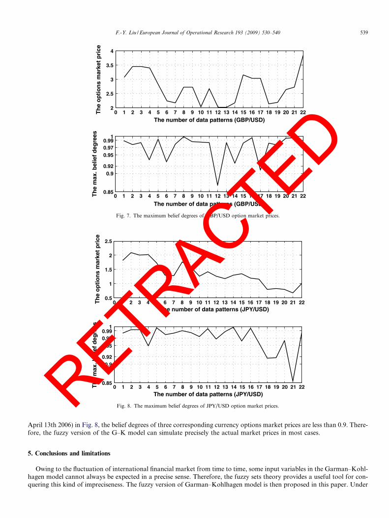
the daily market price or any price from this 90%-level interval as the option price for their later use at any a trade datefrom 3-16-2006 to 4-18-2006. From Figs. 3–5, it can be seen that most of market prices lie in the closed interval with beliefdegree 95% and thus the market prices are closer to the theory prices based on the G–K model with belief degree 1. Theleft-end and right-end of the closed intervals with the different belief degrees are obtained by Eqs. (22) and (23) and illus-trated in Figs. 3–5.
Figs. 6–8 illustrate the maximum belief degrees of EUR/USD, GBP/USD and JPY/USD currency options market pricesto the theory price. The top diagrams illustrate the market prices vary with the different trade dates from 3-16-2006 to 4-18-2006. Correspondingly, the second diagrams illustrate the belief degrees of the market prices. According to Figs. 6–8, thebelief degrees of most of the market prices are from 0.95 to 1 and the belief degrees of only a few market prices are between0.90 and 0.95. Specially, only No. 17 (i.e. April 7th 2006) in Fig. 6, No. 12 (i.e. March 31th 2006) in Fig. 7 and No. 21 (i.e.ACT

0 1 2 3 4 5 6 7 8 9 10 11 12 13 14 15 16 17 18 19 20 21 221

1.5

2

2.5

3

3.5

The number of data patterns (EUR/USD)

Th

e o

pti

on

s m

arke

t p

rice

0 1 2 3 4 5 6 7 8 9 10 11 12 13 14 15 16 17 18 19 20 21 220.88

0.9

0.92

0.95

0.97

0.991

The number of data patterns (EUR/USD)

Th

e m

ax. b

elie

f d

egre

es

Fig. 6. The maximum belief degrees of EUR/USD option market prices.

RETR

0 1 2 3 4 5 6 7 8 9 10 11 12 13 14 15 16 17 18 19 20 21 222

2.5

3

3.5

4

The number of data patterns (GBP/USD)

Th

e o

pti

on

s m

arke

t p

rice

0 1 2 3 4 5 6 7 8 9 10 11 12 13 14 15 16 17 18 19 20 21 220.85

0.90.92

0.950.970.99

1

The number of data patterns (GBP/USD)

Th

e m

ax. b

elie

f d

egre

es

Fig. 7. The maximum belief degrees of GBP/USD option market prices.

0 1 2 3 4 5 6 7 8 9 10 11 12 13 14 15 16 17 18 19 20 21 220.5

1

1.5

2

2.5

The number of data patterns (JPY/USD)

Th

e o

pti

on

s m

arke

t p

rice

0 1 2 3 4 5 6 7 8 9 10 11 12 13 14 15 16 17 18 19 20 21 220.85

0.90.92

0.950.970.99

1

The number of data patterns (JPY/USD)

Th

e m

ax. b

elie

f d

egre

es

Fig. 8. The maximum belief degrees of JPY/USD option market prices.


RETRACTED

April 13th 2006) in Fig. 8, the belief degrees of three corresponding currency options market prices are less than 0.9. There-fore, the fuzzy version of the G–K model can simulate precisely the actual market prices in most cases.

5. Conclusions and limitations

Owing to the fluctuation of international financial market from time to time, some input variables in the Garman–Kohl-hagen model cannot always be expected in a precise sense. Therefore, the fuzzy sets theory provides a useful tool for con-quering this kind of impreciseness. The fuzzy version of Garman–Kohlhagen model is then proposed in this paper. Under


the considerations of the fuzzy domestic and foreign interest rates, fuzzy volatility and fuzzy spot exchange rate, the Euro-pean call currency option price turns into a fuzzy number. This makes the financial investors who can pick any option pricewith an acceptable belief degree for their later use.

The proposed fuzzy version of the Garman–Kohlhagen model is tested with the daily market price data of EUR/USD,GBP/USD and JPY/USD currency options. The experimental results illustrate that the currency option market prices lie inthe closed interval with belief degree 90% and most of market prices lie in the closed interval with belief degree 95%. Thus,the market prices are closer to the theory prices based on the Garman–Kohlhagen model. In addition, according to Figs. 6–8, the belief degrees of most of the market prices are between 0.95 with 1.

Since the price of an American call currency option is the same as the price of a European call currency option, themethodology proposed in this paper may also be applicable for the American call currency option pricing.

In the usual approach, there are two ways to describe the input variable in the Garman–Kohlhagen model. One assumesthe input variable as a constant, and another one assumes the stochastic variable. The theories for modeling the random-ness and fuzziness cannot be substituted for each other. Therefore, the methodology for considering the fuzzy input var-iable will be totally different from that of considering the stochastic input variable. In fact, it is still possible to take intoaccount the imprecisely stochastic input variable for the options pricing. Under this situation, the imprecisely stochasticinput variable may be regarded as a fuzzy random variable. Therefore, it means that the fuzzy input variable is the corre-sponding consideration of the constant input variable under fuzzy environment, and the imprecisely stochastic input var-iable (i.e. the fuzzy random variable) is the corresponding consideration of stochastic input variable under fuzzyenvironment. Only the fuzzy input variable is under investigated in this paper as the beginning step for studying the cur-rency options pricing by using the fuzzy sets theory. The study for the imprecisely stochastic input variable will be thefuture research.

According to Figs. 6–8, the belief degrees of a few market prices are between 0.90 with 0.95. Specially, only No. 17 (i.e.April 7th 2006) in Fig. 6, No. 12 (i.e. March 31th 2006) in Fig. 7 and No. 21 (i.e. April 13th 2006) in Fig. 8, the beliefdegrees of three corresponding currency options market prices are less than 0.9. Therefore, on one hand, the fuzzy versionof the Garman–Kohlhagen model can simulate the actual market prices in most cases. On the other hand, owing to theoriginal Garman–Kohlhagen model is created under some assumptions, the fuzzy model based on Garman–Kohlhagenmodel may be imprecise when the assumptions are not true. The study for creating more precise fuzzy currency optionspricing model will be future research.

Furthermore, it will be useful if a comparison of fuzzy number theory with more commonly used confidence intervals instatistics is provided. The key point is that how to determine the probability distributions of input variables and currencyoptions prices prior to making the comparison. This comparison as the further research is valuable in the future.

References

Amin, K., Jarrow, R., 1991. Pricing foreign currency options under stochastic interest rates. Journal of International Money and Finance 10, 310–329.Andres, J., Terce�nno, G., 2004. Estimating a fuzzy term structure of interest rates using fuzzy regression techniques. European Journal of Operational

Research 154, 804–818.Bates, D., 1996. Jumps and stochastic volatility: exchange rate processes implicit in deutsche mark options. Review of Financial Studies 9, 69–107.Black, F., Scholes, M., 1973. The pricing of options and corporate liabilities. Journal of Political Economics 81, 637–659.Bollen, P.B.N., Rasiel, E., 2003. The performance of alternative valuation models in the OTC currency options market. Journal of International Money

and Finance 22, 33–64.Ekvall, N.L., Jennergren, P., Naslund, B., 1997. Currency option pricing with mean reversion and uncovered interest parity – a revision of the Garman–

Kohlhagen model. European Journal of Operational Research 100, 41–59.Garman, M.B., Kohlhagen, S.W., 1983. Foreign currency option values. Journal of International Money and Finance 2, 231–237.Heston, S., 1993. A closed-form solution for options with stochastic volatility with applications to bond and currency options. Review of Financial Studies

6, 327–344.Lim, G.C., Lye, J.N., Martin, G.M., Martin, V.L., 1998. The distribution of exchange rate returns and the pricing of currency options. Journal of

International Economics 45, 351–368.Ribeiro, R.A., Zimmermann, H.-J., Yager, R.R., Kacprzyk, J., 1999. Soft computing in financial engineering. Physica-Verlag, Heidelberg.Rosenberg, J.V., 1998. Pricing multivariate contingent claims using estimated risk-neutral density functions. Journal of International Money and Finance

17, 229–247.Santos, E., 1970. Fuzzy algorithms. Information and Control 17, 326–339.Sarwar, G., Krehbiel, T., 2000. Empirical performance of alternative pricing models of currency options. The Journal of Futures Markets 20 (2), 265–291.Wu, Hsien-Chung, 2005. European option pricing under fuzzy environment. International Journal of Intelligent System 20, 89–102.Zadeh, L.A., 1965. Fuzzy sets. Information and Control 8 (3), 338–353.Zadeh, L.A., 1968. Fuzzy algorithms. Information and Control 12, 94–102.Zadeh, L.A., 1975. The concept of a linguistic variable and its application to approximate reasoning I. Information Sciences 8 (3), 199–251.

RETRACTED

retracted: pricing currency options based on fuzzy techniques

Documents