retrieval of leaf area index in different vegetation types ...atlas.massey.ac.nz/courses/142405/lai...

www.elsevier.com/locate/rse

Remote Sensing of Environment 86 (2003) 120–131

Retrieval of leaf area index in different vegetation types using high

resolution satellite data

Roberto Colomboa,*, Dario Bellingerib, Dante Fasolinic, Carlo M. Marinob

a Institute for Environment and Sustainability, Joint Research Centre of the European Commission, TP 262, Via E. Fermi, s/n 21020 Ispra, Varese, ItalybDISAT Universita Degli Studi di Milano-Bicocca, Piazza della Scienza 1, 20126 Milan, Italy

cERSAF Ente Regionde per i Servizi all, Agricoltura e alle Foreste della Lombardia, Via Ponchielli 2/4, Milan, Italy

Received 21 March 2002; received in revised form 18 February 2003; accepted 8 March 2003

Abstract

With the successful launch of the IKONOS satellite, very high geometric resolution imagery is within reach of civilian users. In the 1-m

spatial resolution images acquired by the IKONOS satellite, details of buildings, individual trees, and vegetation structural variations are

detectable. The visibility of such details opens up many new applications, which require the use of geometrical information contained in the

images. This paper presents an application in which spectral and textural information is used for mapping the leaf area index (LAI) of

different vegetation types. This study includes the estimation of LAI by different spectral vegetation indices (SVIs) combined with image

textural information and geostatistical parameters derived from high resolution satellite data. It is shown that the relationships between

spectral vegetation indices and biophysical parameters should be developed separately for each vegetation type, and that the combination of

the texture indices and vegetation indices results in an improved fit of the regression equation for most vegetation types when compared with

one derived from SVIs alone. High within-field spatial variability was found in LAI, suggesting that high resolution mapping of LAI may be

relevant to the introduction of precision farming techniques in the agricultural management strategies of the investigated area.

D 2003 Elsevier Science Inc. All rights reserved.

Keywords: LAI; IKONOS; SVIs; Texture indices

1. Introduction The information content of panchromatic and multispec-

The high spatial resolution of IKONOS satellite images

allows for various environmental applications, such as

mapping, agriculture, forestry, and emergency response.

The satellite sensor can generate 1-m panchromatic and 4-

m multiband images with off-nadir viewing of up to 60.25jfor better revisit rate and stereo capabilities. The panchro-

matic imagery has a spectral wavelength interval ranging

from 0.45 to 0.9 Am while the multispectral imagery

includes four bands in the blue, green, red and near-infrared

part of the spectrum (0.45–0.52, 0.52–0.60, 0.63–0.69, and

0.76–0.90 Am). This very high resolution satellite imagery

provides a new source of data for monitoring agricultural

production, potentially providing information with respect

to the development of crops during the growing season.

0034-4257/03/$ - see front matter D 2003 Elsevier Science Inc. All rights reserv

doi:10.1016/S0034-4257(03)00094-4

* Corresponding author. DISAT Universita Degli Studi di Milano-

Bicocca, Piazza della Scienza 1, 20126 Milan, Italy. Tel.: +39-0264482848;

fax: +39-0264482895.

E-mail address: [email protected] (R. Colombo).

tral satellite images may be useful in large-scale quantitative

assessment of biophysical attributes, such as leaf area index

(LAI), which are key inputs in models describing biosphere

processes. The characterisation of the biosphere is a key step

for understanding biological and physical processes associ-

ated with vegetation, for developing ecosystem productivity

models and for computing the mass and energy exchange

between soil, vegetation and atmosphere (Bonan, 1993; Liu,

Chen, Cihlar, & Park, 1997; Sellers, Mintz, Sud, & Dalcher,

1986). Currently, ecosystem models require either field

validation of simulated LAI, or remotely sensed estimates

of LAI to initiate them (Running et al., 1999). Leaf area

index measurements are critical for improving the perform-

ance of such models over large areas and this has prompted

investigations of the relationship between ground-measured

LAI and spectral vegetation indices (SVIs) derived from

satellite-measured data (Chen & Cihlar, 1996; Fassnacht,

Gower, MacKenzie, Nordheim, & Lillesand, 1997; Nemani,

Pierce, Running, & Band, 1993; Spanner, Pierce, Peterson,

& Running, 1990).

ed.

R. Colombo et al. / Remote Sensing of Environment 86 (2003) 120–131 121

Although LAI can be directly or indirectly measured by

several methods (see e.g. Gower, Kucharik, & Norman,

1999; White, Asner, Nemani, Privette, & Running, 2000),

its spatial and temporal distribution is usually investigated

using remotely sensed data. The simplest and most practical

way is to investigate the relationships between LAI and SVI

values by means of regression models. Such relationships

usually result in different mathematical forms with empirical

coefficients that vary, depending primarily on vegetation

type (e.g., Chen, Rich, Gower, Norman, & Plummer, 1997;

Turner, Cohen, Kennedy, Fassnacht, & Briggs, 1999).

Moreover, these relationships are affected by several factors,

such as background reflectance, crown closure, orientation

and aggregation of leaf elements, branches, stand age and

difference in chlorophyll concentration. A considerable

scatter in LAI–SVI relationships is usually found when

the ground pixels observed by the sensor include a combi-

nation of canopy reflectances, originating from different

types of vegetation with a variable amount of understory

(Chen & Cihlar, 1996; Frankin, 1986). The red (R, 0.63–

0.69 Am), Near InfraRed (NIR, 0.76–0.90 Am), Shortwave

Infrared (SWIR, 1.55–1.75 Am) and Middle Infrared bands

(MIR, 2.08–2.35 Am) are the typically used bands in SVI

computation, and their response in producing LAI maps is

discussed in many studies (e.g., Baret, Guyot, Begue,

Maurel, & Podaire, 1988; Brown, Chen, Leblanc, & Cihlar,

2000; Fassnacht et al., 1997; Nemani et al., 1993).

When the analysis is to be conducted at field scale, very

high resolution satellite data can be a useful input for

different environmental applications. Field scale refers to a

geometrical resolution able to resolve intra-field variability

of crop condition. Traditional agriculture considers a field as

a homogeneous unit, while the exploitation of very high

geometrical resolution satellite data may allow detecting

within-field spatial variability of biophysical parameters,

useful in agricultural management (Moran, Inoue, & Barnes,

1997). Information regarding within-field spatial variability

is necessary in precision farming techniques in order to

increase canopy uniformity, and thus to improve crop yield

and quality (Barnes, Pinter, Moran, & Clarke, 1997; Garcia

Cidad & Vrindts, 2001; Johnson, Roczen, & Youkhana,

2001).

Individual cover types generally show a strong relation-

ship between LAI and SVIs. Therefore, high spatial reso-

lution imagery should allow for the retrieval of better LAI–

SVI relationships as compared to low resolution imagery, in

which each pixel may be made up of many land cover types.

Using IKONOS data, the scattering effect of mixed land

cover classes on the spectral data may be reduced.

LAI retrieval by means of IKONOS data is usually

conducted by regression models with SVIs (e.g. Johnson

et al., 2001) without including any additional geometrical

information. However, texture information provided by high

geometrical resolution aerial and satellite data can poten-

tially be used as additional information related to the spatial

canopy architecture that, combined with spectral data, might

improve the LAI description (Weiss et al., 2001; Wulder,

Franklin, & Lavigne, 1996, Wulder, Le Drew, Franklin, &

Lavigne, 1998).

In this study, different LAI estimates for five vegetation

type classes, obtained from spectral vegetation indices and

textural information, are discussed. The potential of very

high resolution data for LAI retrieval is outlined, and the

LAI spatial variability within the different vegetation types

is analyzed.

2. Methods

Three techniques, based on SVIs coupled with texture

indices and geostatistics, are applied in order to retrieve LAI

of different agricultural crops using IKONOS data acquired

almost simultaneously with ground measurements. LAI

values, derived from the LAI-2000 Plant Canopy Analyzer

(LI-COR, 1992, Lincoln, NE), were plotted versus SVI data,

and versus a combination of SVI and texture information.

The test site area is located in the S. Colombano region

(Italy), characterized by a landscape encompassing hilly

vineyards and flat alluvial areas of the Po river plain mainly

devoted to agricultural crops and intensive poplar plantations.

2.1. Ground-based LAI measurements

The LAI-2000 instrument was used in different vegeta-

tion types to derive LAI indirectly. LAI measurements were

collected in a test area investigated in the DUSAF project

(Destinazione d’Uso dei Suoli Agricoli e Forestali), coordi-

nated by ERSAL (Ente Regionale di Sviluppo Agricolo

della Lombardia) and focused on precise land use and land

cover mapping.

LAI-2000 measures the gap fraction P(h) in five zenith

angle (h) ranges with midpoints of 7j, 23j, 38j, 53j and

67j. LAI is determined by inverting simple radiative trans-

fer model foliage information according to Welles and

Norman (1991). This indirect LAI estimate specifically

represents an effective leaf area index for the agricultural

crops and an effective plant area index, including branch

components, for deciduous forests. The assumption of a

random spatial distribution of the leaves as made in the

model inversion is generally satisfied for these crops. Where

a nonrandom spatial distribution of canopy foliage is

observed, an accurate description of gap size is essential

to avoid large errors in LAI estimation (Chen et al., 1997;

Gower et al., 1999).

LAI was calculated according to Gower and Norman

(1991) from the LAI-2000 gap fraction measurements:

LAI ¼ 2

Z p=2

0

ln½1=PðhÞ�cosh sinh dh

LAI measurements were collected in late May 2001,

under diffuse radiation conditions at sunset in one sensor

Fig. 1. Example of a corn field with two LAI measurements (left). Schematic presentation of a 3� 3 pixel kernel of the multispectral IKONOS image (12� 12

m), illustrating the crossing of crop rows (diagonal dashed lines) by the transect.

Table 1

Spectral vegetation indices used in LAI retrieval

SVI Algorithm

NDVI NIR� R

NIRþ R

SR NIR

R

SAVI NIR� aR� c

NIRþ Rþ Lð1þ LÞ

PVI NIR� aR� c

a2 þ 1ffiffiffiffiffiffiffiffiffiffiffiffiffia2 þ 1

p

ARVI NIR� rb

NIRþ rb; rb ¼ R� cðB� RÞ

EVI NIR� R

NIRþ C1*R� C2*Bþ C3

*G

B, R, and NIR represent the IKONOS DN data in blue, red and infrared

bands. Parameters a, c, L, and c regard respectively the gain and the offset

of the soil line, the SAVI term (set equal to 0.5) and the ARVI term (set

equal to 1). The coefficients adopted in the EVI algorithm are C1 = 6.0,

C2 = 7.5, C3 = 1, and G = 2.5.

R. Colombo et al. / Remote Sensing of Environment 86 (2003) 120–131122

mode, and using a 45j view cap. LAI was measured along

ground transects in five different vegetation types: soybean,

corn, vineyards, poplar plantation (plantation) and decidu-

ous forest (forest). Measurements were performed in differ-

ent fields, at different phenological stages and with different

canopy heights, and were also collected within the same

field to determine the within-field LAI spatial variation.

Twenty-eight crop fields were investigated for a total of 39

LAI measurements with 12, 7, 8, 6, and 6 measurements in

corn, soybean, plantations, vineyards, and forest, respec-

tively.

Each LAI measurement was obtained by combining two

parallel transects, diagonally crossing the crop rows accord-

ing to the schema presented in Fig. 1.

The transect length and the spatial interval between

ground samples were fixed for all vegetation types, and a

single LAI value was thus obtained by averaging 10

samples, 5 collected along the first 10-m transect and 5

collected coming back along the parallel one. With a

distance of 2 m between the samples, consecutive samples

of the LAI-2000 instrument are overlapping when the

canopy height is greater than 70 cm. The distance between

two transects was set to a minimum of 3 m. Such a planning

scheme was designed in order to characterise a window of

3� 3 pixels on the multispectral IKONOS image (144 m2)

and, depending on the canopy height, different crop field

areas were sampled.

A single IKONOS panchromatic-multispectral image

was used for all sites. IKONOS data were acquired on 29

May 2001 under clear sky conditions. The view angle was

15j off-nadir. Raw digital number (DN), re-scaled to the full

11-bit range, was used in this study. As a consequence, in

the absence of the re-scaling parameters it was impossible to

compute the calibrated radiance from the original data

(Holtman and Rigopoulos, Space Imaging, personal com-

munication). IKONOS images were initially georeferenced

by an image-to-image technique, using as a master the

digital orthophoto provided by ERSAL. A first-order poly-

nomial was used with a nearest neighbour resampling,

obtaining a registration accuracy of 0.6 pixel for the multi-

spectral images.

The LAI-2000 measurements were geolocated on the

IKONOS images as follows. During field work, transect

starting points were directly positioned on the printed,

georeferenced panchromatic IKONOS image with a com-

pass for measuring their azimuth. Each transect was digi-

Fig. 2. IKONOS multispectral image (a) and dissimilarity image (b). Highest dissimilarity values correspond to poplar plantations and vineyards, which are

well distinguished from other crops.


tised and then located on the georeferenced multispectral

image to define the kernel window. It is assumed that these

LAI field measurements can be considered as representative

of a window of 3� 3 pixels in the multispectral IKONOS

image. The coefficient of variation in these windows was

generally less than 5% for each band, showing little sub-

window heterogeneity.

2.2. LAI–SVI relationships

Initially, six SVIs were directly computed from DN data

to analyse the relationship with LAI (Table 1). Normalised

difference vegetation index (NDVI) (Rouse & Haas, 1973),

simple ratio (SR) (Jordan, 1969), soil adjusted vegetation

index (SAVI) (Huete, 1988), perpendicular vegetation index

(PVI) (Richardson & Wiegand, 1977), and atmospherically

resistant vegetation index (ARVI) (Kaufman & Tanre, 1992)

were selected as representative of intrinsic, soil adjusted and

atmospherically corrected indices. The last three spectral

indices were included in the study to analyse their effects on

Fig. 3. The different spatial variability pattern within the deciduous forest and

reducing the background and atmospheric effects in LAI

mapping.

The enhanced vegetation index (EVI) (Huete, Justice, &

van Leeuwen, 1999) used with the coarse resolution

MODIS data was also investigated.

A series of field-sampled bare soils pixels were selected

on the panchromatic band that reflect the broad band albedo

of the scene in order to determine the a and b parameters of

the so-called ‘‘soil line’’ for computing SAVI and PVI.

Initially, all the LAI measurements (N = 39) were

plotted against the SVIs in order to compute the coef-

ficient of determination (r2) of the regression equation. A

window of 3� 3 pixels was initially used in each spectral

band to determine the spatial homogeneity by statistical

parameters.

The analysis was then conducted for each vegetation

type, plotting the LAI measurements against the SVIs.

The r2 for each LAI–SVI relationship was then re-

computed using the SVI values based on mean reflectances

of different windows sizes of 6� 6 and 9� 9 pixels.

poplar plantation data is well reproduced by the semivariogram function.

Fig. 4. Relationship between all measured LAI in different vegetation types and NDVI.

Table 2

Summary table of the coefficient of determination (r2) for LAI retrievals

computed using the three different approaches

Vegetation SVI Texture analysis Geostatistical parameter

typeNDVI NDVI/

dissimilarity

NDVI +

sill

NDVI +

range

NDVI +

range + diss

Forest/

plantation

0.60 0.73 0.65 0.72 0.76

Forest n.s. 0.73 n.s. n.s. n.s.

Plantation 0.79 0.81 0.79 0.8 0.82

Vineyards 0.74 0.98 n.s. n.s. n.s.

Soybean 0.74 0.74 – – –

Corn 0.80 0.80 – – –

All data 0.33 0.62 – – –

n.s.: not significant at p= 0.05; – : not computed since any additional

information is provided by texture.


2.3. LAI retrieval by SVIs and texture analysis

Image texture is a quantification of the spatial variation

of image tone values, which can be related to spatial

distribution of vegetation. The above-ground organisation

of forest elements is represented in texture, which is

supplementary to the spectral image data and may provide

an additional information source. Image texture may be

related to a variety of statistical measurements that charac-

terise the relationships between neighbouring pixels. Homo-

geneity, contrast, and entropy are measures related to the

specific textural characteristics of the image, while dissim-

ilarity, mean, and standard deviation characterise the com-

plexity and the nature of grey level transitions defined in the

co-occurrence matrix (Wulder et al., 1998).

The approach for LAI determination based on texture

component is subject to the hypothesis that the image spatial

information can be represented in simple texture statistics,

which are a substitute for the structure of the forest vege-

tation or the distribution of LAI, and that the definition of

the forest structure can result in better estimates of LAI in

patchy stands.

The texture indices were calculated for the IKONOS

panchromatic band at the maximum spatial resolution of 1

m. To appreciate the texture of the vegetation, three different

window sizes were employed (3� 3, 6� 6, 9� 9 pixels). A

series of textural variables were tested and the best results in

terms of r2 were obtained by using the dissimilarity index.

Dissimilarity (D) was computed according to the formula:

D ¼Xn�1

i;j¼0

Pi;jji� jj

where P is the probability for the cell i, j (row and column

numbers, respectively). Pi,j is computed as follows

Pi;j ¼Vi;j

Xn�1

i;j¼0

Vi;j

where Vi,j is the DN value in the cell i,j of the image window.

Dissimilarity was observed to reflect a texture measure

that is high when the field region investigated has a high

amount of spatial local variation related to structural char-

acteristics of the image (e.g., crops raw and cover, crops

height and shadowing effects, discontinuous urban fabric)

(Fig. 2).

The dissimilarity image was resampled at a 4-m reso-

lution, in order to integrate texture information with the

spectral vegetation indices previously derived from multi-

spectral data.

The relationship between the combined SVI-texture data

versus LAI was tested by performing multiple linear regres-

sions, with LAI as dependent variables and SVI/dissimilar-

ity as independent indices.

2.4. LAI retrieval by SVIs, texture and geostatistical

parameters

Geostatistics is a useful technique whenever the property

of interest behaves as a spatially correlated variable. Several

authors have used geostatistical parameters to extract struc-

tural, biophysical, and forest damage information (Bruni-

quel-Pinel & Gastellu-Etchegorry, 1998; Chica Olmo &

Abarca Hernandez, 2000; Franklin, Wulder, & Lavigne,

1996; Levesque & King, 1999; Weiss et al., 2001; Wulder

Fig. 5. Relationships between LAI and NDVI for individual vegetation types.


et al., 1996; ) from digital data. The central tool of geo-

statistics is the variogram, which is used to examine the

spatial continuity of a regionalized variable as a function of

distance and direction. A variogram is a plot of the semi-

variances at different distances (lag), which is computed as

the sum of squared differences between all possible pairs of

points separated by the chosen distance. Semivariance (c(h))was computed according to:

cðhÞ ¼ 1

2m

Xm1¼1

½zðxiÞ � zðxi þ hÞ�2

where m is the number of pairs of pixels separated by the

same lag(h) and z(xi) is the DN value at the xi position.

Semivariance is thus obtained for each lag and plotted

against the lag.

Semivariance thus represents the degree of spatial

dependence between samples. The main properties defining

the variogram are the sill, the range, and the nugget, which

relate to the height of the variogram, the distance to reach

the sill, and the positive y-intercept, respectively.

For measurements of LAI in forest and plantations, a

window size of 50� 50 pixels on the IKONOS panchro-

matic band was selected, since it allows analysis of homo-

geneous areas with respect to crop type and is large enough

to allow the calculation of a significant semivariance plot.

Omni-directional semivariograms were then computed, and

Fig. 6. Trend of the coefficient of determination co

nugget, range, and sill were determined from the fitted

mathematical spherical models. The graphical representa-

tion of the average semivariance of several pixel pairs at

each lag distance (h) computed for plantations and forest

classes is shown in Fig. 3.

A spherical model was adopted, even though plantations

showed a periodic pattern due to their typical rows (Bruni-

quel-Pinel & Gastellu-Etchegorry, 1998). The geostatistical

parameters were computed and employed in multivariate

linear regression with the vegetation indices and the dissim-

ilarity image.

3. Results and discussion

For all SVIs, the relationship with LAI shows a positive

correlation with a low coefficient of determination. The

overall relationship between all LAI measurements and

SVIs appears inadequate for mapping LAI. Fig. 4 shows,

as an example, the correlation between LAI and NDVI

(r2 = 0.33).

The large scatter is caused, in part, by the grouping of all

vegetation types. The observed degree of uncertainty would

greatly compromise the utility of the relationship for LAI

mapping at this detailed scale. Due to the heterogeneity of

the group of data, one LAI–SVI relationship is not adequate

mputed for the six SVIs used in this study.


for mapping LAI across all vegetation types. The detected

heterogeneity is probably of the same order of magnitude as

the heterogeneity detectable within a coarse resolution cell.

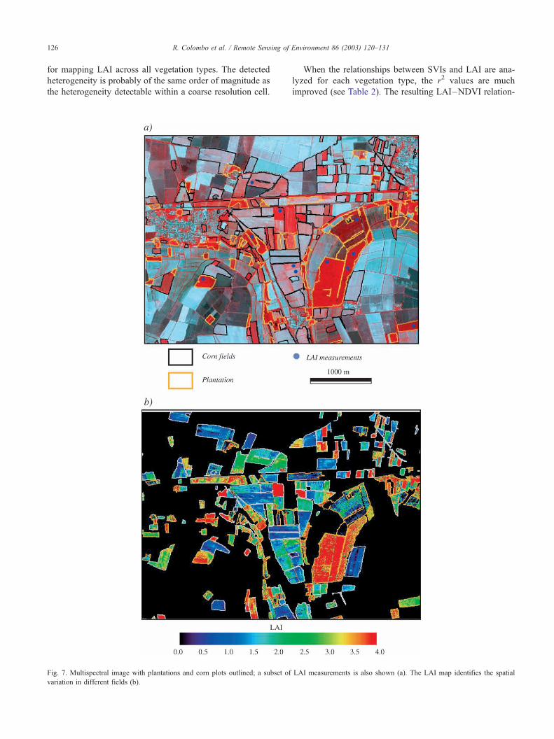
Fig. 7. Multispectral image with plantations and corn plots outlined; a subset of

variation in different fields (b).

When the relationships between SVIs and LAI are ana-

lyzed for each vegetation type, the r2 values are much

improved (see Table 2). The resulting LAI–NDVI relation-

LAI measurements is also shown (a). The LAI map identifies the spatial


ships show the great increase in r2 in the agricultural crops

(Fig. 5).

When the relationship between LAI and NDVI is com-

puted for all vegetation types grouped together, without

including the forest class, a decrease in r2 to a value of 0.25

was found.

At the same time, the scatter of the relationships is still

relatively high in forests, due to their high internal hetero-

geneity. The investigated forest showed the highest LAI

values, with a low SVI variability, and the 3� 3 pixel

window generally corresponds to an area with different tree

heights and canopy architecture.

It was difficult to define the most appropriate SVI for

mapping LAI of each crop. There is not much variation

among SVIs, with relatively high r2 in most cases. EVI was

found to have the same performance as NDVI for all crops

analyzed. In Fig. 6, the coefficient of determination com-

puted for the different SVIs is reported.

Fig. 8. On the left, the true colour IKONOS images and on the right, the LAI map

areas are shown in black.

The low variation among the SVIs in these correlation

coefficients may be related to the fact that each crop was

sampled at different phenological stages, ranging from very

low cover to a high degree of vegetation amount. This may

result in a deterioration of the performance for soil line-

based indices. No improvement for the background effect

was determined using SAVI index, while PVI does worse in

plantation stands and better in forest. Moreover, no im-

provements were found by using SVIs that minimise the

atmospheric and background effects. ARVI may not have

been successful since the terrain morphology shows low

relative relief and, therefore, spatial differences in upwelling

sky irradiance and path radiance are low.

It should be noted that the regression equations between

SVIs and LAI were obtained by fitting a linear relation-

ship, although other studies have shown the nonlinearity of

NDVI/LAI (e.g. Chen & Cihlar, 1996; Myneni, Nemani, &

Running, 1997).

s derived for poplar plantation (b) and corn vegetation type (d). The masked

Fig. 9. Coefficient of determination of the relationships LAI–NDVI as estimated from different window sizes for each vegetation type.


The LAI spatial variations of corn and plantations fields,

for a sector of the investigated area of about 15 km2, are

shown in Fig. 7. LAI is mapped from NDVI data and allows

observation of the different behaviour of the plantations in

the abandoned meandering river system. A large LAI range

characterizes the corn, with fields varying from 0.5 to 4.5

m2/m2.

Examples of detailed LAI maps for the intensive planta-

tion and for corn crops show the within-field variation of

LAI (Fig. 8).

Spatial LAI variations are very evident at the field scale

as intra-culture variations characterizing different crop

stages. In a corn field, the within-field variation of the

ground-based LAI measurements ranged from 0.8 to 2.0.

This heterogeneity is related to variations in crop develop-

ment due to a uniform management (irrigation, chemical

treatments) applied to a portion of terrain showing hetero-

geneous edaphic conditions. Other studies have also shown

a high spatial variability of LAI and other biophysical

parameters within crop fields detected by remote sensing

techniques (Barnes et al., 1997; Castagnoli & Dosso, 2001;

Johnson et al., 2001; Yang & Anderson, 1999). These

studies suggest that precision farming techniques might

usefully incorporate data on local LAI variation, computed

from IKONOS data. The performance of areas with low LAI

could potentially be improved through a differentiated treat-

Fig. 10. Values of coefficient of determination computed for the different veg

ment, and LAI maps could be used to formulate manage-

ment recommendations during the early stages of growth.

The analysis was finally conducted computing different

window sizes starting from the SVI values, and a substantial

stability was observed when the relationships were com-

puted using window sizes of 3� 3, 6� 6 and 9� 9 pixels.

The application of different kernel sizes did not influence

the coefficient of determination of the LAI–SVI relation-

ships (Fig. 9).

Window sizes greater than nine pixels generally include

surrounding fields with different crop types. Thus, the field

sampling scheme for measuring LAI may be considered

appropriate to represent the vegetation spatial variability

detected by high geometric resolution satellite data.

Spatial heterogeneity in canopy architecture was ana-

lyzed in the LAI mapping by introducing texture indices.

The best indicator of texture was found to be the dissim-

ilarity index as computed on a 6� 6 pixel window from

panchromatic data. The combination of the dissimilarity

index and vegetation indices resulted in an increase of the

coefficient of determination for most of the vegetation types

when compared with that derived from SVIs alone (Fig. 10).

A large increase in r2 for the overall relationship (from

0.33 to 0.62) was achieved when texture information was

included in the analysis, suggesting a useful way to avoid

possible problems related to class definitions with an

etation types using spectral and textural information of IKONOS data.


automatic land cover stratification. The addition of a texture

index as a covariate in the multiple regressions has an effect

similar to doing a classification before developing the LAI–

SVI relationships.

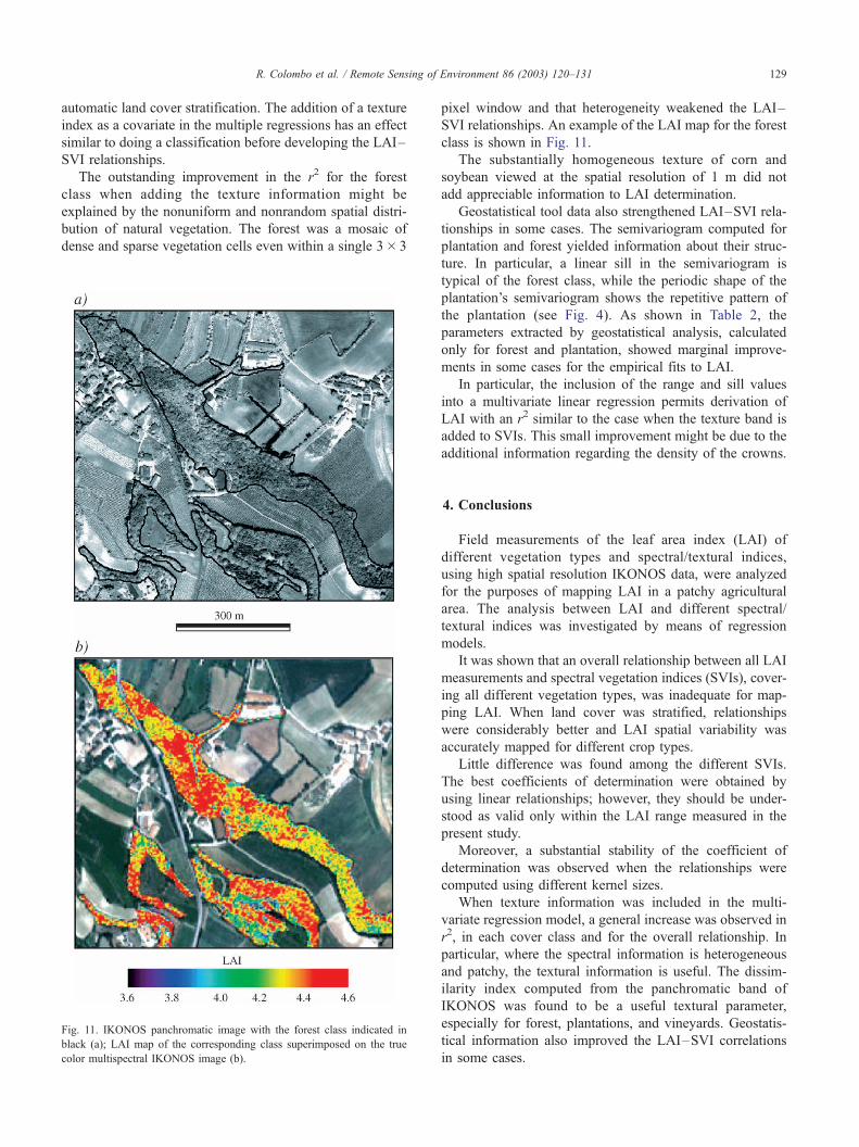
The outstanding improvement in the r2 for the forest

class when adding the texture information might be

explained by the nonuniform and nonrandom spatial distri-

bution of natural vegetation. The forest was a mosaic of

dense and sparse vegetation cells even within a single 3� 3

Fig. 11. IKONOS panchromatic image with the forest class indicated in

black (a); LAI map of the corresponding class superimposed on the true

color multispectral IKONOS image (b).

pixel window and that heterogeneity weakened the LAI–

SVI relationships. An example of the LAI map for the forest

class is shown in Fig. 11.

The substantially homogeneous texture of corn and

soybean viewed at the spatial resolution of 1 m did not

add appreciable information to LAI determination.

Geostatistical tool data also strengthened LAI–SVI rela-

tionships in some cases. The semivariogram computed for

plantation and forest yielded information about their struc-

ture. In particular, a linear sill in the semivariogram is

typical of the forest class, while the periodic shape of the

plantation’s semivariogram shows the repetitive pattern of

the plantation (see Fig. 4). As shown in Table 2, the

parameters extracted by geostatistical analysis, calculated

only for forest and plantation, showed marginal improve-

ments in some cases for the empirical fits to LAI.

In particular, the inclusion of the range and sill values

into a multivariate linear regression permits derivation of

LAI with an r2 similar to the case when the texture band is

added to SVIs. This small improvement might be due to the

additional information regarding the density of the crowns.

4. Conclusions

Field measurements of the leaf area index (LAI) of

different vegetation types and spectral/textural indices,

using high spatial resolution IKONOS data, were analyzed

for the purposes of mapping LAI in a patchy agricultural

area. The analysis between LAI and different spectral/

textural indices was investigated by means of regression

models.

It was shown that an overall relationship between all LAI

measurements and spectral vegetation indices (SVIs), cover-

ing all different vegetation types, was inadequate for map-

ping LAI. When land cover was stratified, relationships

were considerably better and LAI spatial variability was

accurately mapped for different crop types.

Little difference was found among the different SVIs.

The best coefficients of determination were obtained by

using linear relationships; however, they should be under-

stood as valid only within the LAI range measured in the

present study.

Moreover, a substantial stability of the coefficient of

determination was observed when the relationships were

computed using different kernel sizes.

When texture information was included in the multi-

variate regression model, a general increase was observed in

r2, in each cover class and for the overall relationship. In

particular, where the spectral information is heterogeneous

and patchy, the textural information is useful. The dissim-

ilarity index computed from the panchromatic band of

IKONOS was found to be a useful textural parameter,

especially for forest, plantations, and vineyards. Geostatis-

tical information also improved the LAI–SVI correlations

in some cases.


The derived relationships allowed highlighting of high

within-field spatial variability of LAI in the investigated

area. High spatial resolution mapping of LAI with IKONOS

data may be particularly useful in applications such as

precision agriculture, where information on LAI variation

is relevant to management decisions.

Acknowledgements

This work was supported by Regione Lombardia (Italy)

grant to Dr. Fasolini. We gratefully acknowledge Michele

Meroni (Di.S.A.F.Ri, Universita della Tuscia, Viterbo) for

his suggestions and Tracy d’Alton who helped improve the

manuscript. We would like to thank the anonymous

reviewers for their useful comments.

References

Baret, F., Guyot, G., Begue, A., Maurel, P., & Podaire, A. (1988). Com-

plementarity of middle infrared with visible and near-infrared reflectance

for monitoring wheat canopies. Remote Sens. Environ., 26, 213–225.

Barnes, E. M., Pinter, P. J., Moran, M. S., & Clarke, T. R. (1997). Remote

sensing techniques for the integration of crop models with GIS. Proc.

89th Annual Meeting of the American Society of Agronomy. Anaheim,

CA: Crop Science Society of America and Soil Science Society of

America.

Bonan, G. B. (1993). Importance of leaf area index and forest type when

estimating photosynthesis in boreal forests. Remote Sens. Environ., 43,

303–314.

Brown, L., Chen, J. M., Leblanc, S. G., & Cihlar, J. (2000). A shortwave

infrared modification to the simple ratio for LAI retrieval in boreal

forests: An image and model analysis. Remote Sens. Environ., 71,

16–25.

Bruniquel-Pinel, V., & Gastellu-Etchegorry, J. P. (1998). Sensitivity of

texture of high resolution images of forest biophysical and acquisition

parameters. Remote Sens. Environ., 65, 61–85.

Castagnoli, A., & Dosso, P. (2001). Servizi ad alta tecnologia per la viti-

coltura di precisione. L’Informatore Agrario, 18, 57–62.

Chen, J. M., & Cihlar, J. (1996). Retrieving leaf area index for boreal

conifer forests using Landsat TM images. Remote Sens. Environ., 55,

153–162.

Chen, J. M., Rich, P. M., Gower, S. T., Norman, J. M., & Plummer, S.

(1997). Leaf area index of boreal forests: Theory, techniques and meas-

urements. J. Geophys. Res., 102, 29429–29443.

Chica Olmo, M., & Abarca Hernandez, F. (2000). Computing geostatistical

image texture for remotely sensed data classification. Comput. Geosci.,

26, 373–383.

Fassnacht, K. S., Gower, S. T., MacKenzie, M. D., Nordheim, E. V., &

Lillesand, T. M. (1997). Estimating the leaf area index of north central

Wisconsin forest using the Landsat Thematic Mapper. Remote Sens.

Environ., 61, 229–245.

Frankin, J. (1986). Thematic mapper analysis of coniferous forest structure

and composition. Int. J. Remote Sens., 10, 1287–1301.

Franklin, S. E., Wulder, M. A., & Lavigne, M. B. (1996). Automated

derivation of geometric window sizes for use in remote sensing digital

image texture analysis. Comput. Geosci., 22(6), 665–673.

Garcia Cidad, V., & Vrindts, E. (2001). Use of very high resolution satellite

images for precision farming: Recommendations on nitrogen fertilisa-

tion. In M. Owe, G. D’Urso, & E. Zilioli (Eds.), Remote Sensing for

Agriculture, Ecosystems, and Hydrology II. SPIE Proc. ( pp. 24–33).

Bellingham, WA, USA: SPIE.

Gower, S. T., & Norman, J. M. (1991). Rapid estimation of leaf area index

for forests using LI-COR LAI-2000. Ecology, 72, 1896–1900.

Gower, S. T., Kucharik, C. J., & Norman, J. M. (1999). Direct and indirect

estimation of leaf area index, fapar, and net primary production of

terrestrial ecosystems. Remote Sens. Environ., 70, 29–51.

Huete, A. R. (1988). A soil adjusted vegetation index (SAVI). Remote Sens.

Environ., 25, 295–309.

Huete, A. R., Justice, C. O., & van Leeuwen, W. (1999). MODIS Vege-

tation Index (MOD 13) Algorithm Theoretical Basis Document

(ATBD-MOD-13) version 3, available at http://eospso.gsfc.nasa.gov/

ftp_ATBD/REVIEW/MODIS/ATBD_MOD_13/atbd_mod_13.pdf.

Johnson, L. F., Roczen, D., & Youkhana, S. (2001). Vineyard canopy

density mapping with Ikonos satellite imagery. Third International Con-

ference on Geospatial Information in Agriculture and Forestry, Denver,

Colorado. 10 pp.

Jordan, C. F. (1969). Derivation of leaf area index from quality of light on

the forest floor. Ecology, 50, 663–666.

Kaufman, Y. J., & Tanre, D. (1992). Atmospherically Resistant Vegetation

Index (ARVI) for EOS-MODIS. IEEE Trans. Geosci. Remote Sens., 30,

261–270.

Levesque, J., & King, D. J. (1999). Airborne digital camera image semi-

variance for evaluation of forest structural damage at an acid mine site.

Remote Sens. Environ., 68, 112–124.

LI-COR (1992). LAI-2000 plant canopy analyzer instruction manual. Lin-

coln, NE: LI-COR.

Liu, J., Chen, J. M., Cihlar, J., & Park, W. M. (1997). A process-based

Boreal ecosystem productivity simulator using remote sensing inputs.


Moran, M. S., Inoue, Y., & Barnes, E. M. (1997). Opportunities and lim-

itations for image-based remote sensing in precision crop management.


Myneni, R. B., Nemani, R. R., & Running, S. W. (1997). Estimation of

global leaf area index and absorbed par using radiative transfer models.

IEEE Trans. Geosci. Remote Sens., 4, 1380–1393.

Nemani, R., Pierce, L., Running, S. W., & Band, L. (1993). Forest ecosys-

tem processes at the watershed scale: Sensitivity to remotely sensed leaf

area index estimates. Int. J. Remote Sens., 14(13), 2519–2534.

Richardson, A. J., & Wiegand, C. L. (1977). Distinguishing vegetation

from soil background information. Photogramm. Eng. Remote Sens.,

43, 1541–1552.

Rouse, J. W., & Haas, R. H. (1973). Monitoring vegetation systems in the

great plain with ERTS. Third ERTS Symposium, vol. 1 ( pp. 309–317).

Washington, DC: NASA.

Running, S. W., Baldocchi, D. D., Turner, D. P., Gower, S. T., Bakwin,

P. S., & Hibbard, K. A. (1999). A global terrestrial monitoring net-

work integrating tower fluxes, flask sampling, ecosystem modeling

and EOS satellite data. Remote Sens. Environ., 70, 108–127.

Sellers, P. J., Mintz, Y., Sud, Y. C., & Dalcher, A. (1986). A simple bio-

sphere model (SiB) for use within general circulation models. J. Atmos.

Sci., 43, 505–531.

Spanner, M. A., Pierce, L. L., Peterson, D. L., & Running, S. W. (1990).

Remote sensing of temperate coniferous forest leaf area index. The

influence of canopy closure, understory vegetation and background

reflectance. Int. J. Remote Sens., 11, 95–111.

Turner, D. P., Cohen, W. B., Kennedy, R. E., Fassnacht, K. S., & Briggs,

J. M. (1999). Relationship between leaf area index and Landsat TM

Spectral Vegetation Indices across three temperate zone sites. Remote

Sens. Environ., 70, 52–68.

Weiss, M., Beaufort, L., Baret, F., Allard, D., Bruguier, N., & Marloie,

O. (2001). Mapping Leaf Area Index measurements at different

scales for the validation of large swath satellite sensors: First results

of the VALERI project. (http://www.147.100.05/valeri/documents//

valeri-aussois.pdf).

Welles, J. M., & Norman, J. M. (1991). Instrument for indirect measure-

ment of canopy architecture. Agron. J., 83, 818–825.

White, M. A., Asner, G. P., Nemani, R. R., Privette, J. L., & Running, S. W.

(2000). Measuring fractional cover and leaf area index in arid ecosys-

http:\\eospso.gsfc.nasa.gov\ftp_ATBD\REVIEW\MODIS\ATBD_MOD_13\atbd_mod_13.pdf

http:\\www.147.100.05\valeri\documents\\valeri-aussois.pdf


tems: Digital camera, radiation transmittance, and laser altimetry meth-

ods. Remote Sens. Environ., 74, 45–75.

Wulder, M. A., Franklin, S. E., & Lavigne, M. B. (1996). High spatial

resolution optical image texture for improved estimation of forest stand

leaf area index. Can. J. Remote Sens., 22(4), 441–449.

Wulder, M. A., Le Drew, E. F., Franklin, S. E., & Lavigne, M. (1998).

Aerial image texture information in the estimation of northern decidu-

ous and mixed wood forest leaf area index (LAI). Remote Sens. Envi-

ron., 64, 64–76.

Yang, C., & Anderson, G. L. (1999). Airborne videography to identify

spatial plant growth variability for grain sorghum. Precis. Agric.,

1(1), 67–79.

retrieval of leaf area index in different vegetation types ...atlas.massey.ac.nz/courses/142405/lai...

Documents