retrieval of trace gases vertical profile in the lower
TRANSCRIPT

Alma Mater Studiorum - Universita degli Studi di Bologna
DOTTORATO DI RICERCA
Modellistica Fisica per la Protezione dell’Ambiente
Ciclo XX
Settore scientifico disciplinare di afferenza: FIS/06
Retrieval of trace gases vertical profile
in the lower atmosphere combining
Differential Optical Absorption Spectroscopy
with radiative transfer models
Presentata da: Relatore:Dott.ssa Elisa Palazzi Chiar.mo Prof. Rolando Rizzi
Co-relatore:Dott. Giorgio Giovanelli
Coordinatore:Chiar.mo Prof. Ezio Todini
Esame finale anno 2008

Contents
List of Figures 5
List of Tables 9
Acronyms and abbreviations 13
Introduction 17
1 Absorption and scattering of UV and visible solar radiationin the atmosphere 23
1.1 Composition and structure of the Earth’s atmosphere . . . . . 24
1.2 Absorption in the UV/visible solar spectrum . . . . . . . . . . 28
1.2.1 The Beer-Bouguer-Lambert law . . . . . . . . . . . . . 30
1.3 Scattering of solar radiation . . . . . . . . . . . . . . . . . . . 33
1.3.1 Rayleigh scattering . . . . . . . . . . . . . . . . . . . . 35
1.3.2 Mie scattering . . . . . . . . . . . . . . . . . . . . . . . 39
1.3.3 Geometric scattering . . . . . . . . . . . . . . . . . . . 40
1.4 Visibility . . . . . . . . . . . . . . . . . . . . . . . . . . . . . . 41
1.4.1 Gas absorption effects on visibility . . . . . . . . . . . 43
2 Multiple AXis Differential Optical Absorption Spectroscopy(MAX-DOAS) 47
2.1 The absorption spectroscopy for atmospheric measurements . 47
2.2 The DOAS technique . . . . . . . . . . . . . . . . . . . . . . . 49
2.2.1 The Fraunhofer reference spectrum . . . . . . . . . . . 51
2.2.2 The Ring effect . . . . . . . . . . . . . . . . . . . . . . 52
2.3 MAX-DOAS: the geometric approach . . . . . . . . . . . . . . 53
2.4 MAX-DOAS: the radiative transfer approach . . . . . . . . . . 54
2.4.1 The intercomparison exercise for MAX-DOAS calcula-tions . . . . . . . . . . . . . . . . . . . . . . . . . . . . 57
3

4 CONTENTS
3 The Monte Carlo Radiative Transfer Model PROMSAR 71
3.1 Radiometric quantities . . . . . . . . . . . . . . . . . . . . . . 71
3.2 Radiative transfer equation . . . . . . . . . . . . . . . . . . . . 74
3.2.1 The Monte Carlo approach to the RTE . . . . . . . . . 76
3.3 Description of the PROMSAR RTM . . . . . . . . . . . . . . 79
3.3.1 Backward Monte Carlo technique . . . . . . . . . . . . 80
3.3.2 The photon history tracking . . . . . . . . . . . . . . . 81
3.3.3 Input description of the PROMSAR code . . . . . . . . 92
3.3.4 Variance reducing techniques . . . . . . . . . . . . . . 93
3.4 Sample applications of the PROMSAR code . . . . . . . . . . 94
3.4.1 Transmittance/irradiance/radiance calculations . . . . 94
3.4.2 Zenith-sky and off-axis Air Mass Factor calculations . . 99
4 Remote sensing and the retrieval problem 109
4.1 Atmospheric remote sensing . . . . . . . . . . . . . . . . . . . 111
4.1.1 The beginnings . . . . . . . . . . . . . . . . . . . . . . 111
4.1.2 Atmospheric remote sensing methods . . . . . . . . . . 111
4.2 Information aspects in retrieval methods . . . . . . . . . . . . 112
4.2.1 Formal statement of the problem . . . . . . . . . . . . 113
4.2.2 Linear problems without measurement error . . . . . . 115
4.2.3 Linear problems with measurement error . . . . . . . . 116
4.3 Error analysis in retrieval methods . . . . . . . . . . . . . . . 117
4.3.1 Characterisation . . . . . . . . . . . . . . . . . . . . . 117
4.3.2 Error analysis . . . . . . . . . . . . . . . . . . . . . . . 120
4.4 The Chahine inversion method . . . . . . . . . . . . . . . . . . 121
4.4.1 Application of the Chahine inversion method . . . . . . 121
5 Case study: retrieval of nitrogen dioxide and ozone verticalprofiles in the boundary layer 127
5.1 The measurement site . . . . . . . . . . . . . . . . . . . . . . 127
5.2 The instrumental set-up . . . . . . . . . . . . . . . . . . . . . 129
5.3 Data analysis and results . . . . . . . . . . . . . . . . . . . . . 129
5.3.1 Meteorological conditions on 29 October 2006 . . . . . 130
5.3.2 Slant column measurements of NO2 and ozone . . . . . 131
5.3.3 AMF calculation and aerosol setting . . . . . . . . . . 136
5.3.4 The retrieval of NO2 and ozone vertical profiles . . . . 138
Conclusions 151
Appendix 155

CONTENTS 5
References 161

6 CONTENTS

List of Figures
1.1 Vertical profile of the temperature between the surface and100 km altitude as defined in the U.S. Standard Atmosphere. . 26
1.2 Spectrum of solar radiation at the top of the atmosphere andat sea level. . . . . . . . . . . . . . . . . . . . . . . . . . . . . 30
1.3 Absorption cross section of NO2 and O3 in the wavelengthinterval (200-650) nm. . . . . . . . . . . . . . . . . . . . . . . 32
1.4 Depletion of the radiant intensity in traversing an absorbingmedium. . . . . . . . . . . . . . . . . . . . . . . . . . . . . . . 33
1.5 Size parameter α as a function of wavelength of the incidentradiation and particle radius. . . . . . . . . . . . . . . . . . . 35
1.6 Scattering area coefficient K as a function of size parameterα for nonabsorbing spheres with a refractive index of 1.33. . . 36
1.7 Rayleigh scattering: polar diagram of scattered intensity. . . . 38
1.8 Mie scattering: polar diagram of scattered intensity. . . . . . . 39
1.9 Ray paths inside a droplet that lead to the formation of arainbow. . . . . . . . . . . . . . . . . . . . . . . . . . . . . . . 40
1.10 Change of radiation intensity along a beam. . . . . . . . . . . 41
1.11 Extinction coefficients due to NO2 and O3 absorption whenT=298 K and pa=1013 hPa. . . . . . . . . . . . . . . . . . . . 44
2.1 The paths of scattered solar radiation through the atmosphere. 50
2.2 Solar irradiance at the top of the atmosphere. . . . . . . . . . 52
2.3 Fraunhofer lines in the near UV/visible part of the solar spec-trum. . . . . . . . . . . . . . . . . . . . . . . . . . . . . . . . . 52
2.4 Observation geometries for ground-based passive DOAS. . . . 55
2.5 Simulated slant column densities of NO2 and CHOH for dif-ferent input profiles (zenith-looking DOAS). . . . . . . . . . . 56
2.6 Modelled vertical optical depth with respect to Rayleigh scat-tering and normalised radiance (including ozone absorption)as a function of wavelength. . . . . . . . . . . . . . . . . . . . 63
7

8 LIST OF FIGURES
2.7 Box-AMFs for zenith-looking geometry at a solar zenith angleof 70. . . . . . . . . . . . . . . . . . . . . . . . . . . . . . . . 64
2.8 Box-AMFs for 360 nm as a function of altitude. . . . . . . . . 682.9 Box-AMFs for 577 nm as a function of altitude. . . . . . . . . 692.10 Box-AMFs for 360 nm, an elevation angle of 2 and a SZA of
80 as a function of altitude for different azimuth angles. . . . 70
3.1 Emission spectra for blackbodies with different temperatures. . 723.2 The extraterrestrial solar irradiance. . . . . . . . . . . . . . . 733.3 Single scattering of direct solar radiation and multiple scat-
tering of diffuse radiation. . . . . . . . . . . . . . . . . . . . . 743.4 Normalized blackbody spectra representative of the sun and
Earth. . . . . . . . . . . . . . . . . . . . . . . . . . . . . . . . 753.5 Rayleigh phase function. . . . . . . . . . . . . . . . . . . . . . 853.6 Comparison between the numerical values obtained for the
Rayleigh phase function and the analytical values computedfor the central point of each cosine interval. . . . . . . . . . . . 87
3.7 Comparison between the numerical values obtained for theMie phase function and the analytical values computed forthe central point of each cosine interval. . . . . . . . . . . . . 89
3.8 Examples of reflection and refraction. . . . . . . . . . . . . . . 973.9 Refracted slant path through the atmosphere. . . . . . . . . . 993.10 NO2 vertical profile provided by the 1976 U.S. Standard at-
mospheric model. . . . . . . . . . . . . . . . . . . . . . . . . . 1023.11 NO2 vertical profile between 0 and 2 km provided by the 1976
U.S. Standard atmospheric model. . . . . . . . . . . . . . . . . 1023.12 Nitrogen dioxide air mass factors at 440 nm computed with
the PROMSAR model for a stratospheric and a troposphericvertical profile of the absorber. . . . . . . . . . . . . . . . . . . 105
3.13 Nitrogen dioxide air mass factors at 440 nm computed withthe PROMSAR model for a stratospheric and a troposphericvertical profile of the absorber and for four off-axis angles (20,40, 60, 80). . . . . . . . . . . . . . . . . . . . . . . . . . . . 108
4.1 The nature of inverse problems. . . . . . . . . . . . . . . . . . 1104.2 Time series of slant column densities of NO2 at sunrise and
sunset during 1987, at Lauder, New Zealand. . . . . . . . . . . 1234.3 Calculated air mass factors for assumed 5-km-thick slabs of
NO2, for November, 45 S. . . . . . . . . . . . . . . . . . . . . 1244.4 Retrieved NO2 profiles and fitting errors (no NO2 chemistry). 1254.5 Retrieved NO2 profiles and fitting errors (NO2 chemistry). . . 125

LIST OF FIGURES 9
5.1 Map of the Castel Porziano area. . . . . . . . . . . . . . . . . 1285.2 Picture of the TROPOGAS spectrometer components. . . . . 1305.3 Daily mean temperatures from 25 to 31 October 2006 mea-
sured at the Pratica di Mare station. . . . . . . . . . . . . . . 1325.4 Daily averages of wind direction and speed measured at the
Pratica di Mare station from 25 to 31 October 2006. . . . . . . 1325.5 Surface weather map at 12 UTC 29 October 2006. . . . . . . . 1335.6 500 hPa weather map at 12 UTC 29 October 2006. . . . . . . 1345.7 MAX-DOAS NO2 slant column densities measured at Castel
Porziano on 29 October 2006. . . . . . . . . . . . . . . . . . . 1355.8 MAX-DOAS NO2 slant column densities measured at Castel
Porziano on 29 October 2006 at 84, 87, 88, and 89 off-axisdirections. . . . . . . . . . . . . . . . . . . . . . . . . . . . . . 136
5.9 MAX-DOAS O3 slant column densities measured at CastelPorziano on 29 October 2006. . . . . . . . . . . . . . . . . . . 137
5.10 Box-AMFs for 440 nm as a function of altitude (from 0 to 2km). . . . . . . . . . . . . . . . . . . . . . . . . . . . . . . . . 139
5.11 Box-AMFs for 440 nm as a function of altitude (from 0.1 to10 km). . . . . . . . . . . . . . . . . . . . . . . . . . . . . . . 140
5.12 NO2 and O3 concentration profiles and vertical column densi-ties in the boundary layer deduced from a set a MAX-DOASmeasurements taken at four off-axis angles and at the az-imuthal direction of 115. . . . . . . . . . . . . . . . . . . . . 141
5.13 Averaging kernels - 1. . . . . . . . . . . . . . . . . . . . . . . . 1425.14 Averaging kernels - 2 . . . . . . . . . . . . . . . . . . . . . . . 1435.15 NO2 tropospheric columns from OMI on 29 October 2006. . . 1445.16 Diurnal evolution of nitrogen dioxide vertical profile at dif-
ferent altitude levels, as deduced by means of the retrievalinversion algorithm. . . . . . . . . . . . . . . . . . . . . . . . . 145
5.17 Backward trajectories ending at Castel Porziano on 29 Octo-ber 2006. . . . . . . . . . . . . . . . . . . . . . . . . . . . . . . 146
5.18 Backward trajectories ending at Castel Porziano on 25, 26, 27,28, 29, and 30 October 2006. . . . . . . . . . . . . . . . . . . . 148
5.19 Measured and recalculated nitrogen dioxide slant column den-sities at 84, 87, 88, and 89. . . . . . . . . . . . . . . . . . . 149
5.20 Percent errors distribution of the measured and simulatedslant column densities. . . . . . . . . . . . . . . . . . . . . . . 149

10 LIST OF FIGURES
List of Tables
1.1 Volume mixing ratios of fixed gases in the lowest 100 km ofthe Earth’s atmosphere. . . . . . . . . . . . . . . . . . . . . . 24
1.2 Volume mixing ratios of some variable gases in three atmo-spheric regions . . . . . . . . . . . . . . . . . . . . . . . . . . 25
1.3 Wavelengths of absorption in the visible and UV spectra byseveral gases. . . . . . . . . . . . . . . . . . . . . . . . . . . . 31
1.4 Meteorological ranges resulting from gas scattering, gas ab-sorption, particle scattering, particle absorption. . . . . . . . . 43
1.5 Extinction coefficients and meteorological ranges due to NO2
absorption at selected wavelength intervals and concentration. 44
2.1 Lower boundaries and vertical extensions of the atmosphericlayers selected for the box-AMF calculation. . . . . . . . . . . 60
2.2 Overview on the intercomparison participating models andsome important properties. . . . . . . . . . . . . . . . . . . . . 61
2.3 Wavelengths and ozone cross sections used in the RTM com-parison exercise. . . . . . . . . . . . . . . . . . . . . . . . . . . 62
2.4 Aerosol properties for the different test cases of the RTM com-parison exercise. . . . . . . . . . . . . . . . . . . . . . . . . . . 62
2.5 Overview of the solar zenith angles, the elevation and the rel-ative azimuth angles of the telescope used in the RTM com-parison exercise. . . . . . . . . . . . . . . . . . . . . . . . . . . 62
3.1 Cosine probability table for Rayleigh scattering. . . . . . . . . 86
3.2 Comparison between the numerical (Monte Carlo) and analyt-ical values of the Rayleigh phase function, and their standarddeviation. . . . . . . . . . . . . . . . . . . . . . . . . . . . . . 88
3.3 Comparison between the numerical (Monte Carlo) and ana-lytical values of the Mie phase function, and their standarddeviation. . . . . . . . . . . . . . . . . . . . . . . . . . . . . . 90
11

12 LIST OF TABLES
3.4 Transmittance comparison between MODTRAN and PROM-SAR RTMs. . . . . . . . . . . . . . . . . . . . . . . . . . . . . 96
3.5 Irradiance comparison between MODTRAN and PROMSARRTMs. . . . . . . . . . . . . . . . . . . . . . . . . . . . . . . . 97
3.6 Refraction parameters comparison between MODTRAN andPROMSAR RTMs. . . . . . . . . . . . . . . . . . . . . . . . . 98
3.7 Diffuse to global irradiance ratio experiment-PROMSAR com-parison. . . . . . . . . . . . . . . . . . . . . . . . . . . . . . . 100
3.8 Total single- and multiple- scattered radiance comparison be-tween MODTRAN and PROMSAR RTMs. . . . . . . . . . . . 101
3.9 NO2 AMF for single scattering approximation and multiplescattering at 440 nm (1976 U.S. Standard profile for NO2). . . 103
3.10 NO2 AMF for single scattering approximation and multiplescattering at 440 nm (1976 U.S. Standard profile for NO2 be-tween 0-2 km). . . . . . . . . . . . . . . . . . . . . . . . . . . 104
3.11 NO2 AMF for single/multiple scattering at 440 nm and forfour off-axis angles (20, 40, 60, 80). 1976 U.S. Standardprofile for NO2. . . . . . . . . . . . . . . . . . . . . . . . . . . 106
3.12 NO2 AMF for single/multiple scattering at 440 nm and forfour off-axis angles (20, 40, 60, 80). 1976 U.S. Standardprofile for NO2 between 0-2 km. . . . . . . . . . . . . . . . . . 107
5.1 Daily mean meteorological data measured at the Pratica diMare station from 25 to 31 October 2006. . . . . . . . . . . . 131

Acronyms and abbreviations
ACS Absorption Cross Section
AMF Air Mass Factor
CCD Charged Coupled Device
CFC Chlorofluorocarbons
CNR National Research Council
COSPEC COrrelation SPECtrometer
DOAS Differential Optical Absorption Spectroscopy
ENEA Ente per le Nuove Tecnologie, l’Energia e l’Ambiente
ENVISAT ENVIronmental SATellite
EOS Earth Observing System
ERS European Remote Sensing
GASCOD Gas Analyzer Spectrometer Correlating Optical Differences
GDAS Global Data Assimilation System
GOME Global Ozone Monitoring Experiment
GOMOS Global Ozone Monitoring by Occultation of Stars
H-G Henyey-Greenstein
HYSPLIT Hybrid Single-Particle Lagrangian Integrated Trajectory
ISAC Institute of Atmospheric Sciences and Climate
IR Infrared

14 Acronyms and abbreviations
IRIS InfraRed Interferometer Spectrometer
IUGG International Union of Geodesy and Geophysics
LIDAR Light Detection And Ranging
LIMS Limb Infrared Monitor of the Stratosphere
MAX-DOAS Multiple AXis DOAS
MC Monte Carlo
MODTRAN MODerate resolution TRANsmittance
NASA National Aeronautics and Space Administration
NCEP National Centers for Environmental Prediction
NOOA National Oceanic and Atmospheric Administration
OA Off-Axis
OMI Ozone Monitoring Instrument
PROMSAR PROcessing of Multi-Scattered Atmospheric Radiation
RTE Radiative Transfer Equation
RTM Radiative Transfer Model
SAGE-II Stratospheric Aerosol and Gas Experiment-II
SCD Slant Column Density
SCIAMACHY SCanning Imaging Absorption spectroMeter for Atmosphe-ric ChartographY
SIRS Satellite InfraRed Spectrometer
SZA Solar Zenith Angle
TOA Top Of the Atmosphere
TROPOGAS TROPOsheric GAScod
UTC Coordinated Universal Time
UV Ultraviolet

Acronyms and abbreviations 15
VCD Vertical Column Density
VRT Variance Reducing Technique
WMO World Meteorological Organization

16 Acronyms and abbreviations

Introduction
Historically, human activities have always interacted with the atmosphere,but the growth of population and industrialisation in the 19th and 20th cen-tury has led to dramatic changes in the Earth system. Long-term measure-ments have clearly shown that human activities are changing the composi-tion of the Earth’s atmosphere and research has demonstrated the importantconsequences of such changes for climate, human health, and the balance ofecosystems. As a consequence, in the last decades, several efforts have beenmade to develop new observational platforms, to model the future behaviourof the atmosphere, to understand the historic development of climate, tomonitor anthropogenic and natural emissions as well as to collect knowledgefor policy makers to facilitate their decisions.The observational platforms for atmospheric composition comprise severalcomponents such as ground-based measurements (including in-situ, remotesensing and ballon instrumentation), aircraft measurements, satellite mea-surements as well as a data modelling system with assimilation to provide acomprehensive global picture.
Useful measurement techniques for atmospheric trace species should ful-fill at least two main requirements. First, they must be sufficiently sensitiveto detect the species under consideration at their ambient concentration lev-els. This can be a very demanding criterion; for instance, species present atmixing ratios ranging from as low as 0.1 ppt (mixing ratio of 10−13, equiva-lent to about 2 × 10⁶ molecules/cm3) to several ppb (mixing ratio of 10−9)can have a significant influence on the chemical processes in the atmosphere.Thus, detection limits from below 0.1 ppt to the ppb range are required, de-pending on the application. Second, it is equally important for measurementtechniques to be specific, which means that the results of the measurementof a particular species must be neither positively nor negatively influencedby any other trace species simultaneously present in the probed volume ofair. Given the large number of different molecules present at the ppt andppb levels, even in clean air, this is also not a trivial condition.Air monitoring by spectroscopic techniques has proven to be a very useful

18 Introduction
tool to fulfill these desirable requirements as well as a number of other impor-tant properties. During the last decades, many such instruments have beendeveloped which are based on the absorption properties of the constituentsin various regions of the electromagnetic spectrum, ranging from the farinfrared to the ultraviolet. Among them, Differential Optical AbsorptionSpectroscopy (DOAS) has played an important role.
DOAS is an established remote sensing technique for atmospheric tracegases probing, which identifies and quantifies the trace gases in the atmo-sphere taking advantage of their molecular absorption structures in the nearUV and visible wavelengths of the electromagnetic spectrum (from 0.25 µm to0.75 µm). DOAS has a flexible measurement configuration that allows mul-tiple applications (ground-based, airborne and satellite-borne measurementsare possible), and the investigation of the chemistry in the atmosphere toassess the influence of anthropogenic pollution and natural processes.
In the case of passive DOAS, which uses the sun as radiation source, thetrace gases absorption is analyzed and quantified to conclude on the con-centration of the trace gases integrated along the optical path between thesun and the receiver. Therefore, the ability to properly interpret UV/visibleabsorption measurements of atmopsheric constituents using diffuse sunlightdepends crucially on how well the optical path of light collected by the sys-tem is understood.The standard DOAS set-up as used for several decades was that in which ra-diation is collected along the vertical direction (zenith-sky DOAS), and hasits highest sensitivity in the stratosphere, in particular during twilight. Thisis the result of the large enhancement in stratospheric light path at dawnand dusk combined with a relatively short tropospheric path.The sensitivity of the instrument towards tropospheric signals can be stronglyincreased by pointing the telescope to the horizon instead of the zenith (off-axis DOAS). Depending on tropospheric visibility, the light path in the lowerlayers can become very long and increases as the viewing direction approachesthe horizon. At the same time, the light path through the stratosphere is ingood approximation independent of the instrument pointing.The combination of simultaneous measurements at different off-axis angles isreferred to as Multiple AXis DOAS (MAX-DOAS). This recent measurementtechnique is highly sensitive to the absorbers located in the lowest few kilome-ters of the atmosphere and has the advantage that vertical profile informationcan be retrieved by combining the simultaneous off-axis measurements withRadiative Transfer Model (RTM) calculations and inversion techniques.
The motivation for the work presented in this thesis is to retrieve profileinformation for the trace gases nitrogen dioxide (NO2) and ozone (O3) froma set of ground-based UV/visible MAX-DOAS measurements. NO2 is an im-

Introduction 19
portant trace gas in the lower troposphere due to the fact that it is involvedin the production of tropospheric ozone. Ozone and nitrogen dioxide are keyfactors in determining the quality of air with impacts e.g. on human healthand the growth of vegetation. To understand the NO2 and ozone chemistryin more detail not only the concentrations at ground but also the acquisitionof the vertical distribution of the trace gases is necessary. In fact, the budgetof nitrogen oxides and ozone in the atmosphere is determined both by localemissions and non-local chemical and dynamical processes (i.e. diffusion andtransport at various scales) that greatly impact on their vertical and tem-poral distribution: thus a tool to resolve the vertical profile information isreally important.DOAS offers the advantage to be a flexible and relatively simple technique,but it can detect the presence of a trace gas in terms of its integrated concen-tration over the atmospheric path (referred to as the slant column density)and it cannot measure directly the concentration as a function of locationor altitude. To retrieve from such measurements the vertical profile of ab-sorbers, sophisticated radiative transfer calculations have to be performedand inversion schemes applied. It should be intended that this is in strictlyanalogy with many satellite sounders for atmospheric composition.
To derive quantitative information on trace gases distributions, in fact, itis necessary to model the processes intervening along the light path with a Ra-diative Transfer Model (RTM). In particular there is a need for a RTM whichis capable of dealing with such processes, supporting all DOAS geometriesused, and treating multiple scattering events with varying phase functionsinvolved. Deterministic radiative transfer models, for example, are affectedby important limitations: they are often limited to two dimensions (or toplane parallel geometry) neglecting Earth sphericity and multiple scattering,and they cannot model all DOAS geometries which are used to retrieve thevertical profile of absorbers in the atmosphere.
To achieve the multiple goals mentioned above, a statistical approachbased on the Monte Carlo technique can be used. A Monte Carlo RTM gen-erates an ensemble of random photon paths between the light source and thedetector, and uses these paths to reconstruct a remote sensing measurement.Within the present study, the radiative transfer model PROMSAR (PROcess-ing of Multi-Scattered Atmospheric Radiation) has been developed and usedto correctly interpret the slant column densities obtained from MAX-DOASmeasurements. PROMSAR allows to calculate the key processes as the solartransmittance, the irradiance and the radiance obtained by a detector witha specified position, viewing direction and field of view, and for a definedatmospheric scenario. Moreover, PROMSAR includes the Air Mass Factor(AMF) in the calculation, which is the most important output for the inter-

20 Introduction
pretation of remote sensing DOAS measurements, allowing the conversion ofthe slant column density into a vertical column density (the concentration ofthe absorber integrated along the vertical). The air mass factor is definedas the ratio of the slant column density to the vertical column density andcan be used to quantify the enhancement of the light path length within theabsorber layers.
In order to derive the vertical concentration profile of a trace gas fromits slant column measurement, the AMF is only one part in the quantita-tive retrieval process. One indispensable requirement is a robust approachto invert the measurements and obtain the unknown concentrations, the airmass factors being known. For this purpose, in the present thesis, we haveused the Chahine relaxation method. This method had already been used inthe past by several authors to estimate the profile information contained inzenith-sky DOAS measurements using ground-based instruments. The ver-tical resolution of such profiles was, however, relatively low and informationwas limited mainly to the stratospheric part of the profile. Within the studypresented in this thesis, the Chahine inversion method has been modified soas to be applied for inversion of ground-based Multiple AXis DOAS mea-surements and retrieval of the vertical profile of the trace gases of interest inthe lower troposphere.
The outline of this work is as follows: in chapter 1 an overview on thefundamentals of atmospheric chemistry and physics is given, with the aimof introducing some important aspects necessary to understand the researchpresented in this thesis. The main aspects are the structure and compositionof the Earth’s atmosphere, and the processes that concur in the attenuationof solar radiation, such as scattering and absorption by gases and particlesand their effects on visibility.Chapter 2 deals with the DOAS technique and especially the novel MultipleAXis Differential Optical Absorption Spectroscopy (MAX-DOAS). Chapter2 also presents the results of a comparison exercise between radiative transfermodels from different international research groups carried out in 2005/2006,which has been fundamental to point out new aspects connected with thistechnique and the importance to correctly model the MAX-DOAS measure-ments.Chapter 3 outlines the theory of radiative transfer for the atmosphere nec-essary for a proper interpretation of remote sensing data. Moreover, it exten-sively describes the PROMSAR radiative transfer model, which is suitablefor the interpretation of passive DOAS mesurements under different viewingdirections and instrumental settings. This model participated to the inter-

Introduction 21
comparison exercise described in chapter 2. In chapter 3, investigations withthe PROMSAR model for a variety of DOAS geometries, other than thoseshown in chapter 2, are performed and discussed. The development and useof the PROMSAR model has represented a primary goal of this thesis.Chapter 4 illustrates briefly the retrieval theory in the remote sensing con-text, following mainly the work of Rodgers. One particular method, theChahine relaxation method, is described for which an important applicationis discussed in chapter 5.Chapter 5 presents the vertical profile of nitrogen dioxide and ozone fromthe application of the PROMSAR RTM and the Chahine inversion methodto an event of pollutants transport observed at Castel Porziano (near Rome)in October 2006.Conclusions provide the main surveys of this work and give the perspectiveof future applications.

22 Introduction

Chapter 1
Absorption and scattering ofUV and visible solar radiationin the atmosphere
Aerosol particles and gases scatter and absorb radiation as a function ofwavelength. In this chapter, attention will be focused on absorption andscattering of near-ultraviolet and visible solar radiation (from 0.25 to 0.75µm), as these are relevant processes for the Differential Optical AbsorptionSpectroscopy (DOAS) technique. DOAS is a spectroscopic technique whichdetermines the integrated concentration of a trace gas along the light paththat radiation covers in the atmosphere, by means of the trace gas absorptioncharacteristics in the UV/visible spectral ranges. The trace gases presentalong the light path absorb the light at wavelengths which are unique to therespective molecular structure, allowing for the identification of the species.From the strength of the absorption conclusions can be drawn about thetrace gases concentration. Also scattering by molecules and absorption andscattering by aerosol particles have to be taken into account in the processingof recorded spectra by DOAS methodology, because these processes influencethe quantity and intensity of solar radiation that reaches the instrument. TheDOAS technique will be dealt with in detail in chapter 2.
In this chapter, some considerations about visibility are also made, be-cause it is strictly connected to the presence of aerosol particles and moleculesin the atmosphere and their interaction with solar radiation. In pollutedcloud free air the main process reducing visibility is aerosol particle scatter-ing. Particles absorption of visible light is relevant only when soot (blackcarbon and organic matter) is present. Gas absorption is important onlywhen nitrogen dioxide concentrations are high. Instead gas scattering al-ways occurs but it is important relative to other processes only in clean air.

24 1. Absorption and scattering of UV/visible solar radiation
In the first section of this chapter the composition and structure of theatmosphere are briefly described because these aspects are important to theunderstanding of the research presented in this study.
1.1 Composition and structure of the Earth’s
atmosphere
To describe the interaction of the Earth’s atmosphere with solar radiation,it is essential that the atmosphere’s composition is understood. The atmo-sphere is composed of a group of nearly permanent gases and a group of gaseswith variable concentrations. In addition, the atmosphere also contains var-ious solid and liquid particles such as aerosols, water drops, and ice crystals,which are highly variable in space and time. Tables 1.1 and 1.2 list the chem-ical formula and volume ratio for the concentrations of the permanent andvariable gases in the atmosphere, respectively. For variable gases, also anindication of their major sources is given in Table 1.2.
Table 1.1: Volume mixing ratios of fixed gases in the lowest 100 km of the Earth’satmosphere.
Gas name Major remarks Chemical formula Volume mixing ratio% ppmv
Molecular nitrogen Biological N2 78.08 780000Molecular oxygen Biological O2 20.95 209500Argon Inert Ar 0.93 9300Neon Inert Ne 0.0015 15Helium Inert He 0.0005 5Krypton Inert Kr 0.0001 1Xenon Inert Xe 0.000005 0.05
It is apparent from Table 1.1 that nitrogen, oxygen and argon account formore that 99.99% of the permanent gases, which are characterized by the factthat their mixing ratios do not vary very much in time or space. Althoughthe mixing ratio of the permanent gases is constant with increasing altitudes,their partial pressure decreases with increasing altitudes because air pressuredecreases with increasing altitudes and the permanent gases partial pressuresare constant fractions of air pressure. The noble fixed gases possess very longlifetimes against chemical destruction and, hence, are relatively well mixedthroughout the entire homosphere (i.e., below 100 km).

1.1 Composition and structure of the Earth’s atmosphere 25
Table 1.2: Volume mixing ratios of some variable gases in three atmosphericregions: clean troposphere, polluted troposphere, and stratosphere.
Gas name Major sources Chemical Volume mixingand remarks formula ratio (ppbv)
Clean Polluted Stratospheretroposphere troposphere
InorganicWater vapour Volcanic, H2O 3000-4.0·107 (0.5-4.0)·107 3000-6000
evaporationCarbon dioxide Volcanic, CO2 365000 365000 365000
biogenic,anthropogenic
Carbon monoxide Photochemical, CO 40-200 2000-10000 10-60anthropogenicbiogenic
Ozone Photochemical O3 10-100 10-350 1000-12000Sulfur dioxide Photochemical, SO2 0.02-1 1-30 0.01-1
volcanic,anthropogenic
Nitric oxide Anthropogenic NO 0.005-0.1 0.05-300 0.005-10biogenic,lightning,photochemical
Nitrogen dioxide Photochemical NO2 0.01-0.3 0.2-200 0.005-10CFC-12 CF2Cl2 0.55 0.55 0.22OrganicMethane Biogenic, CH4 1800 1800-2500 150-1700
anthropogenicEthane C2H6 0-2.5 1-50 NegligibleEthene C2H4 0-1 1-30 NegligibleFormaldehyde Photochemical HCHO 0.1-1 1-200 NegligibleToluene C6H5CH3 Negligible 1-30 NegligibleXylene C6H4(CH3)2 Negligible 1-30 NegligibleMethyl chloride Biogenic, CH3Cl 0.61 0.61 0.36
anthropogenic
Table 1.2 summarizes the volume mixing ratios of some variable gases inthe clean troposphere, the polluted troposphere (e.g., urban areas), and inthe stratosphere divided also in organic and inorganic gases. Many organicgases have low mixing ratios in the stratosphere because they degrade chem-ically before they reach this region.Most of the constituents of air that are of prime importance in atmosphericchemistry are present in very small concentrations, consequently they arecalled trace constituents. Some of them influence the transmission of solarand terrestrial radiation in the atmosphere and are therefore linked to thephysical climate system. They are key components of biogeochemical cycles;in addition, they determine the “oxidizing capacity” of the atmosphere and,hence, the atmospheric lifetime of biogenic and anthropogenic trace gases.The role of the trace constituents nitrogen dioxide and ozone in urban en-

26 1. Absorption and scattering of UV/visible solar radiation
vironments and in the free troposphere, and the main chemical reactions inwhich these species are involved, are in particular discussed in the Appendix.
The vertical temperature profile for the standard atmosphere is depictedin Fig. 1.1. This profile represents typical conditions in middle latitudes.
Figure 1.1: Vertical profile of the temperature between the surface and 100 kmaltitude as defined in the U.S. Standard Atmosphere (1976) and related atmosphericlayers. Note that the tropopause level is represented for mid-latitude conditions.From [1].
According to the standard nomenclature defined by the International Unionof Geodesy and Geophysics (IUGG) in 1960, the vertical temperature profileis divided into four distinct layers. These are the troposphere, stratosphere,mesosphere and thermosphere. The tops of these layers are respectively calledtropopause, stratopause, mesopause, and thermopause.
The troposphere is characterized by a decrease of temperature with re-spect to height with a typical lapse rate of 6.5 C/km. The temperaturestructure in this layer is a consequence of the radiative balance and the con-vective transport of energy from the surface to the atmosphere. The groundsurface receives energy from the sun daily, heating the ground, but the top ofthe troposphere continuously radiates energy upward, cooling the upper tro-posphere. Convective thermals from the surface transfer energy upward, butas these thermals rise into regions of lower pressure, they expand and cool,

1.1 Composition and structure of the Earth’s atmosphere 27
resulting in a decrease of temperature with increasing height in the tropo-sphere. Virtually all the water vapour, cloud, and precipitation are confinedin this layer.The boundary layer is the region of the troposphere where surface effectsare important. Stull [2] defines the atmospheric boundary layer as “the partof the troposphere that is directly influenced by the presence of the Earth’ssurface, and responds to surface forcings with a time scale of about an houror less”. The boundary layer differs from the “free troposphere” in thatthe temperature profile responds to changes in ground temperatures over aperiod of less than an hour, whereas the temperature profile in the free tro-posphere responds to changes in ground temperatures over a longer period.The boundary layer depth is of the order of 1 km, but varies significantlywith the time of day and with meteorological conditions. The exchange ofchemical compounds between the surface and the free troposphere is directlydependent on the stability of the boundary layer.The tropopause is the upper boundary of the troposphere. Above the tropo-pause base, temperatures are relatively constant with increasing altitude.Tropopause heights are higher (15 to 18 km) over the equator than over thepoles (8 to 10 km). Strong vertical motions over the equator raise the baseof the ozone layer there. Because ozone is responsible for warming above thetropopause, pushing ozone to greater heights over the equator increases thealtitude at which warming begins. Near the poles, downward motions movestratospheric ozone downward, lowering the tropopause height over the poles.Temperatures at the tropopause over the equator are colder than they areover the poles. One reason is that the higher base of the ozone layer over theequator allows tropospheric temperatures to cool to a greater altitude overthe equator than over the poles. A second reason is that lower- and mid-tropospheric water vapour contents are much higher over the equator thanthey are over the poles. Water vapour absorbs thermal-IR radiation emit-ted from the Earth’s surface, preventing that radiation to reach the uppertroposphere. The troposphere, which contains about 85-90% of the atmo-spheric mass, is often dynamically unstable with rapid vertical exchangesof energy and mass being associated with convective activity. Globally, thetime constant for vertical exchanges is of the order of several weeks.
The stratosphere is characterized by an isothermal layer from the tropo-pause to about 20 km from where the temperature increases to the strato-pause. Ozone occurs chiefly in the stratosphere causing the inversion temper-ature. Ozone absorbs the UV radiation from sun (with wavelengths between0.23 and 0.32 µm) and reemits thermal-infrared radiation, heating in thisway the stratosphere. Peak stratospheric temperatures occur at the top ofthe stratosphere (about 50 km) because this is the altitude at which ozone
28 1. Absorption and scattering of UV/visible solar radiation
absorbs the shortest UV wavelengths (about 0.175 µm) reaching the strato-sphere. Although the content of ozone at the top of the stratosphere is low,each ozone molecule can absorb these short wavelengths, increasing the aver-age kinetic energy and, by consequence, temperature of all molecules. ShortUV wavelengths do not penetrate to the lower stratosphere. Ozone densitiesin the stratosphere peak from 25 to 32 km. In addition, thin layers of aerosolare observed to persist for a long period of time within certain altitude rangesof the stratosphere. A typical residence time for material injected in the lowerstratosphere is one to three years.
Like the troposphere the temperatures in the mesosphere decrease withheight from about 50 to about 85 km. Ozone densities are too low in compar-ison with those of oxygen and nitrogen for ozone absorption of UV radiationto affect the average temperature of all molecules in the mesosphere. In thisregion dynamical instability occurs frequently and is characterized by rapidvertical mixing.
Above 85 km and extending upward to an altitude of several hundredkilometers lies the thermosphere where temperatures range from 500 K toas high as 2000 K, depending on the solar activity. In the thermospheretemperatures increase with increasing altitude because O2 and N2 absorbvery short far-UV wavelengths (< 0.1 µm), that in such way do not penetrateto the mesosphere. Vertical exchanges associated with dynamical mixingbecome insignificant, but molecular diffusion becomes an important processthat produces gravitational separation of species according to their molecularor atomic weight.
1.2 Absorption in the UV/visible solar spec-
trum
Before we proceed to discuss the absorption of solar radiation in the near-ultraviolet and visible regions (from 0.25 to 0.75 µm), it would be helpful tointroduce the ways in which a molecule can store various energies.
Any moving particle has kinetic energy as a result of its motion in space.This is known as translational energy. The averaged translational kineticenergy of a single molecule in the X, Y , and Z directions is found to beequal to KT/2, where K is the Boltzmann constant (5.67×10⁻⁸ Wm−2K−4)and T is the absolute temperature.
The molecule which is composed of atoms can rotate about an axisthrough its center of gravity and, therefore, has rotational energy.
The atoms of the molecule are bounded by certain forces in which the
1.2 Absorption in the UV/visible solar spectrum 29
individual atoms can vibrate about their equilibrium positions relative toone other. The molecule therefore will have vibrational energy.
These three molecule energy types are based on a rather mechanical modelof the molecule that ignores the detailed structure of the molecule in termsof nuclei and electrons. It is possible, however, for the energy of a moleculeto change due to a change in the energy state of the electrons of which it iscomposed. Thus, the molecule has electronic energy.
Rotational, vibrational and electronic energies are quantized and takediscrete values only. Absorption and emission of radiation take place whenthe atoms or molecules undergo transitions from one energy state to another.In general, these transitions are governed by selection rules. Atoms canexhibit line spectra associated by electronic energy. Molecules, however, canhave two additional types of energy which lead to complex band systems.
Solar radiation is mainly absorbed in the atmosphere by O2, O3, N2, CO2,H2O, O, and N, although gases which occur in very small quantities also ex-hibit absorption spectra. Absorption spectra due to electronic transitions ofmolecular and atomic oxygen and nitrogen, and ozone occur chiefly in theultraviolet region, while those due to the vibrational and rotational tran-sitions of triatomic molecules such as H2O, O3 and CO2 lie in the infraredregion. Figure 1.2 shows the spectrum of solar radiation reaching the Earth’ssurface for the case of an overhead sun (the lower curve) together with thespectrum of solar radiation incident upon the top of the atmosphere (theupper curve). The area between the two curves represents the depletion ofthe incident radiation during its passage through the atmosphere. The de-pletion is divided into two parts: the unshaded area represents the combinedeffects of backscattering and absorption by clouds and aerosol, and backscat-tering by air molecules, while the shaded area represents the absorption byair molecules. Nearly all the shaded area can be identified with discrete ab-sorption bands, the most important of these being the water vapour bands inthe in the near infrared. There is very little absorption of solar radiation atvisible wavelengths by the gaseous constituents of the atmosphere. This re-markable window in the absorption spectrum coincides with the wavelengthsof maximum solar emission.
Table 1.3 shows the gases that absorbs UV and visible radiation. Ofthe gases listed in Table 1.3 only ozone, NO2 and NO3 absorb in the visiblespectrum. The rest absorbs in the ultraviolet spectrum. Absorption byozone is weak in the visible spectrum and concentrations of the nitrate radical(NO3) are relatively low except at night, when sunlight is absent, as explainedin the Appendix. Probably the most important molecule having substantialabsorption in the visible is NO2, which has significant absorption in theblue region of the spectrum, near 0.430 µm. As already pointed out at the

30 1. Absorption and scattering of UV/visible solar radiation
Figure 1.2: Spectrum of solar radiation at the top of the atmosphere (upper curve)and at sea level (lower curve) for average atmospheric conditions and an overheadsun. The shaded area represents absorption by gaseous constituents, as indicated.
beginning of this chapter, absorption of solar radiation by trace gases is dealtwith, in this thesis, within the field of application of the DOAS technique.In particular, attention will be focused on tropospheric ozone and nitrogendioxide, for which the absorption cross section in the UV/visible part of thesolar spectrum is shown in Fig. 1.3. The part of the solar spectrum between200 and 300 nm primarily is absorbed by the ozone in the upper stratosphereand mesosphere. The regions which consist of the strongest absorption bandsof O3 are called Hartley bands. The bands between 300 and 360 nm are calledHuggins bands, which are not as strong as Hartley bands. O3 also shows weakabsorption bands in the visible (and near infrared) region, called Chappuisbands. The role of nitrogen dioxide in the absorption of solar radiation hasbeen widely discussed in [3].
1.2.1 The Beer-Bouguer-Lambert law
A pencil of radiation traversing a medium will be weakened by its interactionwith matter. If the intensity of radiation Iλ becomes Iλ + dIλ after traversinga thickness ds in the direction of its propagation, as depicted in Fig. 1.4,

1.2 Absorption in the UV/visible solar spectrum 31
Table 1.3: Wavelengths of absorption in the visible and UV spectra by severalgases.
Gas name Chemical formula Absorption wavelengths (µm)Visible/near-UV/far-UV absorbersOzone O3 <0.35, 0.45-0.75Nitrate radical NO3 <0.67Nitrogen dioxide NO2 <0.71Near-UV/far-UV absorbersNitrous acid HONO <0.4Dinitrogen pentoxide N2O5 <0.38Formaldehyde HCHO <0.36Hydrogen peroxide H2O2 <0.35Acetaldehyde CH3CHO <0.345Peroxynitric acid HO2NO2 <0.33Nitric acid HNO3 <0.33Peroxyacetyl nitrogen CH3CO3NO2 <0.3Far-UV absorbersMolecular oxygen O2 <0.245Nitrous oxide N2O <0.24CFC-11 CFCl3 <0.23CFC-12 CF2Cl2 <0.23Methyl chloride CH3Cl <0.22Carbon dioxide CO2 <0.21Water vapour H2O <0.21Molecular nitrogen N2 <0.1
then
dIλ = −kλ · ρ · Iλ · ds, (1.1)
where ρ is the density of the material, and kλ denotes the mass extinctioncross section (in units of area per mass) for radiation of wavelength λ. Themass extinction cross section is the sum of the mass absorption and scatteringcross sections. Thus, the reduction in intensity is caused by absorption in thematerial as well as scattering of radiation by the material. On the other handthe intensity may be strengthened by emission of the material plus multiplescattering from all other directions into the pencil under consideration at thesame wavelength. We define the source function coefficient jλ such that theincrease of the intensity due to emission and multiple scattering is given by:
dIλ = jλ · ρ · ds. (1.2)

32 1. Absorption and scattering of UV/visible solar radiation
Figure 1.3: Absorption cross section (acs) of NO2 (left axis) and O3 (right axis)in the wavelength interval (200-650) nm. A semi-logarithmic scale is used.
Combining Eqs. 1.1 and 1.2 we obtain:
dIλ = −kλ · ρ · Iλ · ds+ jλ · ρ · ds. (1.3)
Moreover it is convenient to define the source function Jλ such that:
Jλ ≡ jλ/kλ. (1.4)
It follows that Eq. 1.3 can be rearranged to yield:
dIλkλ · ρ · ds
= −Iλ + Jλ. (1.5)
When both multiple scattering and emission contributions may be ne-glected (Jλ = 0), and in the absence of scattering by the material, Eq. 1.5only accounts for absorption in the material, and it reduces to the form:
dIλkλ · ρ · ds
= −Iλ, (1.6)
where kλ now represents the mass absorption cross section (or simply absorp-tion coefficient) only. The absorption coefficient is a measure of the fractionof the absorbers per unit wavelength interval that are absorbing radiationat the wavelength in question. If the incident intensity at s = 0 is Iλ(0),as shown in Fig. 1.4, then the emergent intensity at a distance s can beobtained by integrating Eq. 1.6, and is given by:
Iλ(S1) = Iλ(0) · e(−R S10 kλ·ρ·ds) (1.7)

1.3 Scattering of solar radiation 33
Figure 1.4: Depletion of the radiant intensity in traversing an absorbing medium.
Assuming that the medium is homogeneous, then kλ is independent on thedistance s. Thus by defining the path length u
u =
∫ S1
0
ρ · ds, (1.8)
Eq. 1.7 becomes:
Iλ(S1) = Iλ(0) · e(−kλ·µ). (1.9)
This is known as Beer-Bouguer-Lambert law, which states that the decreaseof the radiant intensity traversing a homogeneous absorbing medium is ac-cording to the simple exponential function whose argument is the productof the mass absorption cross section and the path length. The dimensionlessquantity (kλ ·µ) is called the optical depth or optical thickness. It is a measureof the cumulative depletion that the beam of radiation has experienced as aresult of its passage through the medium.It is important to note here that the Beer-Bouguer-Lambert law is the physi-cal low on which the DOAS methodology is based, as will be shown in chapter2. In the DOAS context the quantity u is referred to as slant column density(SCD), and indicates the trace gas concentration integrated along the lightpath.
1.3 Scattering of solar radiation
Most of the light that reaches our eyes comes not directly from its sources butindirectly by the process of scattering. We see diffusely scattered sunlightwhen we look at clouds or at the sky. The land and water surfaces, andthe objects surrounding us are visible through the light that they scatter.

34 1. Absorption and scattering of UV/visible solar radiation
In the atmosphere, we see many colorful examples of scattering generatedby molecules, aerosols, and clouds containing droplets and ice crystals. Bluesky, white clouds, rainbows and haloes, are samples of optical phenomenadue to scattering.
Scattering is a fundamental physical process associated with the lightand its interaction with the matter. By this process, a particle in the pathof an electromagnetic wave continuously abstracts energy from the incidentwave and reradiates that energy in all directions. The particle, therefore,may be thought of as a point source of the scattered energy. The radiationscattered by a particle results from the superposition of all wavelets scat-tered by oscillating dipoles. These dipoles, oscillating at the frequency of theapplied electromagnetic field, produce a secondary field that radiates out inall directions (the scattered field). Particle scattering is a complex problembecause the secondary waves generated by each dipole also act to stimulateoscillations in neighboring dipoles.
It is possible to formulate an expression analogous to Eq. 1.1 for thefraction of parallel beam radiation that is scattered when passing downwardthrough a layer of infinitesimal thickness:
dIλ = −K · A · Iλ · ds, (1.10)
where K is a dimensionless coefficient playing the role of a scattering areacoefficient, and A is the cross-sectional area that the particles in a unit volumepresent to the beam of incident radiation. Thus, K measures the ratio ofthe effective scattering cross section of the particles to their geometric crosssection. For the idealized case of scattering by spherical particles of uniformradius r, the scattering area coefficient K can be prescribed on the basisof theory. It is convenient to express K as a function of a dimensionlesssize parameter α = 2πr/λ, which is a measure of the size of the particles incomparison to the wavelength of the incident radiation. Figure 1.5 shows aplot of α as a function of r and λ.
The scattering area coefficient K depends not only upon the size param-eter but also upon the index of refraction of the particles responsible for thescattering. Figure 1.6, for example, shows K as a function of α for non-absorbing spheres with a refractive index of 1.33. For the special case ofα 1 (the extreme left-hand side of Fig. 1.6), Rayleigh showed that, fora given value of the refractive index, K ∝ α4 and the scattered radiation isevenly divided between the forward and backward hemispheres, as will beshown in section 1.3.1. When α is greater than 50, K ' 2 and the angulardistribution of scattered radiation can be described by the principles of ge-ometric optics, as will be shown in section 1.3.3. For intermediate values of

1.3 Scattering of solar radiation 35
Figure 1.5: Size parameter α as a function of wavelength of the incident radiationand particle radius. From [4].
the size parameter, the scattering phenomenon must be described in termsof the more general theory developed by Mie (section 1.3.2). Within the Mieregime K exhibits the oscillatory behaviour shown in Fig. 1.6. The angulardistribution of scattered radiation is very complicated and varies rapidly withα, with forward scattering predominating over back scattering.
In the atmosphere, the particles responsible for the scattering cover thesizes from gas molecules (10−8 cm) to large raindrops and hail particles (∼1 cm). The relative intensity of the scattering pattern depends strongly onthe ratio of particle size to wavelength of the incident wave.
1.3.1 Rayleigh scattering
When particles are much smaller than the incident wavelength (α 1), thescattering is called Rayleigh scattering, after Lord Baron Rayleigh born JohnWilliam Strutt (1842-1919), who first described the properties of scatteredsunlight by air molecules. Rayleigh’s theoretical work on gas scattering waspublished in 1871 [6]; the English experimental physicist John Tyndall (1820-1893) demonstrated experimentally that the sky’s blue color results fromscattering of visible light by gas molecules and that a similar effect occurswith small particles.
Consider a small homogemeous, isotropic spherical particle whose radiusis much smaller than the wavelength of the incident radiation. The simpli-

36 1. Absorption and scattering of UV/visible solar radiation
Figure 1.6: Scattering area coefficient K as a function of size parameter α fornonabsorbing spheres with a refractive index of 1.33. From [5].
fication introduced by the small size is that the incident radiation producesa homogeneous electric field E0 which generates a dipole configuration onthe small particle. The electric dipole causes an electric field which, in turn,modifies the applied field inside and near the particle; let E be the appliedfield plus the particle own’s field. Let p0 be the induced dipole moment,defined as (electrostatic formula)
p0 = α0 · E0. (1.11)
This relation defines α0, the polarizability of the small particle. Since thedimension of E0 is charge per area, and the dimension of p0 is charge timeslength, α0 has the dimension of a volume. In general, α0 is a tensor. Thismeans that the directions of p0 and E0 coincide only if the field is applied inone of three mutually perpendicular directions.The applied field E0 generates oscillation of an electric dipole in a fixeddirection; the oscillating dipole, in turn, produces an electromagnetic wave,the scattered wave. The scattered electric field in regions which are far awayfrom the dipole is given by
E =1
c21
r
∂2p
∂t2sin γ, (1.12)
where r denotes the distance between the dipole and the observational point,γ the angle between the scattered dipole moment p and the direction ofobservation and c the velocity of light (c = 3 × 10⁸ ms−1). In an oscillatingperiodic field, p may be written in terms of the induced dipole moment as
p = p0 · e−ik(r−ct) (1.13)

1.3 Scattering of solar radiation 37
where k is the wave number (k = 2π/λ). By combining Eqs. 1.11 and 1.13,Eq. 1.12 yields:
E = −E0e−ik(r−ct)
rk2α0 sin γ. (1.14)
Now we consider the scattering of unpolarized sunlight by air molecules. Inthat circumstance, α0 may be considered a scalar. Let the plane defined bythe directions of incident and scattered waves be the reference plane (planeof scattering), with respect to which we define the perpendicular (Er) andparallel (El) components of E. According to Eq. 1.14 we have:
Er = −E0re−ik(r−ct)
rk2α0 sin γ1 (1.15)
El = −E0le−ik(r−ct)
rk2α0 sin γ2, (1.16)
where γ1 = π/2 and γ2 = π/2−Θ, where Θ is the angle between the incidentand scattered waves (the scattering angle). The corresponding intensities(per solid angle ∆Ω) of the incident and scattered radiation may be writtenas
I0 =1
∆Ω
c
4π| E0 |2, I =
1
∆Ω
c
4π| E |2 . (1.17)
Thus, Eqs. 1.15, 1.16 and 1.17 can be expressed in the form of intensities as
Ir = I0rk4α2
0/r2 (1.18)
Il = I0lk4α2
0 cos2 Θ/r2 (1.19)
where Ir and Il are polarized intensity components perpendicular and parallelto the plane of scattering. The total scattered intensity of the unpolarizedsunlight incident on a molecule in the directon of Θ is then
I = Ir + Il = (I0r + I0l cos2 Θ)k4α20/r
2. (1.20)
But for unpolarized sunlight, I0r = I0l = I0/2 and by noting that k = 2π/λ,we get
I =I0r2α2
0
(2π
λ
)4
· 1 + cos2 Θ
2. (1.21)
The term “1” in Eq. 1.21 corresponds to the r-component (electric vectorperpendicular to the plane of scattering), and the term “cos2 Θ” corresponds

38 1. Absorption and scattering of UV/visible solar radiation
to the l-component of the scattered light (electric vector parallel).Figure 1.7 illustrates Eq. 1.21 by the well known scattering diagram. Thepolar diagram represents the total intensity resulting from the sum of thepolarized components contributions perpendicular to plane of drawing (1)and in plane of drawing (cos2 Θ); the light scattered by 90 is fully polarizedin the r-direction (which is not true for anysotropic particles). Equation 1.21
Figure 1.7: Rayleigh scattering: polar diagram of scattered intensity if incidentradiation is unpolarized.
is the original formula derived by Rayleigh, by which the intensity scatteredby a molecule for unpolarized sunlight is proportional to the incident intensityI0 and is inversely proportional to the square of the distance between themolecule and the point of observation. In addition to these two factors,it also depends on the polarizability, the wavelength of the incident wave,and the scattering angle. Scattering of unpolarized sunlight by moleculeshas maxima in the forward (Θ = 0) and backward (Θ = 180) directions,whereas it shows minima in the side directions (Θ = 90 and 270). Theinverse dependence of the scattered intensity on the wavelength to the fourthpower is the foundation for the explanation of the blue of the sky. It isapparent that the λ−4 low causes more of the blue light to be scattered thanthe red, the green and the yellow, and so the sky, when viewed away fromthe sun’s disk appears blue.
It can be seen in Fig. 1.5 that Rayleigh scattering describes not only howvisible radiation is scattered by atmospheric gases, but also how the longerwavelength infrared radiation is scattered by aerosol particles a few tenths ofa micron in size, and how, the even longer microwave radiation is scatteredby cloud droplets and small rain drops.

1.3 Scattering of solar radiation 39
1.3.2 Mie scattering
Larger particles in the atmosphere such as aerosols, cloud droplets, and icecrystals, also scatter sunlight and produce many fascinating optical phenom-ena. However, their single scattering properties are less wavelength-selectiveand depend largely upon the particle size.The dipole mode of the electric field, which leads to the development ofthe Rayleigh scattering theory, is not applicable for particles larger than thewavelength of the incident radiation. Because of the large particle size, theincident beam of light induces high-order modes of polarization configuration,which require more advanced treatment.
Scattering by a spherical particle of arbitrary size has been treated exactlyby Gustav Mie (1868-1957) in 1908 [7], by means of solving the electromag-netic wave equation derived from the fundamental Maxwell equations.
Figure 1.8 illustrates the scattering diagram for scattering by a particlein the Mie regime (α=1.0, 1.5, 3, 6, 20 from top to bottom). The scatteringappears extremely directional in the forward direction: the larger the par-ticle, the more it scatters forward and the greater the forward to backwardasymmetry. The forward component (forward peak) dominates with respectto the backward component because forward moving waves tend to be inphase and this gives a large resultant amplitude whereas backward wavestend to be out of phase and this results in a small resultant amplitude.
Figure 1.8: Mie scattering: polar diagram of scattered intensity. α=1.0, 1.5, 3,6, 20 from top to bottom.
Mie scattering occurs when particles have about the same size as (α ∼ 1)or are greater than (α > 1) the wavelength of radiation. The scattering of

40 1. Absorption and scattering of UV/visible solar radiation
sunlight by particle of haze, smoke, smog, and dust usually falls within thisregime.
1.3.3 Geometric scattering
Particles for which the radius is much greater than the wavelength of light(α 1) fall into the so-called geometric scattering regime. In this case, thescattering can be determined from geometrical optics of reflection, refractionand diffraction. Geometric optics means that the scattering of light can bedetermined by ray tracing, which is also used to determine the optical effectsof lenses and prisms, etc.A good example of the application of geometric optics to particle scatteringis the formation of a rainbow. Figure 1.9 shows the ray paths in a singledroplet that contribute to the formation of a primary rainbow. Light beams
Figure 1.9: Ray paths inside a droplet that lead to the formation of a rainbow.
entering a droplet are first refracted (leading to dispersion), reflected off theback of the droplet and refracted again on leaving the droplet. Independentof the size of the droplet (provided α 1) the angle between the incidentbeam and the return beam is 42 for red light and 40 for the blue light. Notethat not all the light that impinges the droplet goes into forming the rainbow.Much of it is simply reflected off the surface or is refracted and then exits thedroplet in the forward direction. Note also that only one wavelength froma single droplet impinges upon the viewer’s eye. A rainbow appears whenwaves from many droplets hit the eye.For geometric scattering by a sphere, the fraction of incident light that isscattered (expressed in terms of the scattering area coefficient K) is 2. Thismeans that a sphere with radius much greater than the wavelength of lightscatters twice as much energy as it intercepts. This is because light is not

1.4 Visibility 41
only redirected by refraction and reflection (for rays that enter the droplet)but also diffracted about the sphere. Thus a droplet can “intercept” lightwaves that would otherwise pass by.
1.4 Visibility
Visibility is a measure of how far we can see through the air. Perhaps one ofthe most noticeable effects of air pollution is reduction in visibility. Even incleanest air, however, our ability to see along the Earth’s horizon is limitedto a few hundred kilometers by background gases and aerosol particles. Ifwe look up through the sky at night, however, we can discern light fromstars that are millions of kilometers away. The difference is that more gasmolecules and aerosol particles lie in front of us in the horizontal line of sightthan in the vertical one.The regulatory definition of visibility is the meteorological range. It can bedefined as the distance from an observer at which an ideal black object justdisappears when viewed against the horizon sky in daytime. It can better beexplained in terms of the following example. Suppose a perfectly absorbingdark object lies against a white background at a point x0, as shown in Fig.1.10. Because the object is perfectly absorbing, it reflects and emits no visible
Figure 1.10: Change of radiation intensity along a beam. A radiation beamoriginating from a dark object has intensity I=0 at point x0. Over a distance dxthe beam’s intensity increases due to scattering of background light into the beam.This added intensity is diminished somewhat by along the beam and scattering outof the beam.
radiation; thus, its visible radiation intensity (I) at point x0 is zero and itappears black. As a viewer backs away from the object, background whitelight of intensity IB scatters into the field of view, increasing the intensity oflight in the viewer’s direction. Although some of the added background lightis scattered out of the field of view or absorbed along it by gases and aerosol

42 1. Absorption and scattering of UV/visible solar radiation
particles, at some distance away from the object, so much background lighthas entered the path that the viewer can barely discern the black objectagainst the background light.The meteorological range is a function of the contrast ratio which is definedas
Cratio =IB − I
IB, (1.22)
where I is the intensity of object and IB the intensity of background. Thecontrast ratio gives the difference between the background intensity and theintensity of the object in the viewer’s line of sight, all relative to the back-ground intensity. If the contrast ratio is unity, than an object is perfectlyvisible; if it is zero, than the object cannot be distinguished from the back-ground. The meteorological range is the distance from an object at whichthe contrast ratio equals the liminal contrast ratio of 0.02 (2%). The lim-inal contrast ratio is the lowest visually perceptible brightness contrast aperson can see. It obviously varies from individual to individual. In 1924Koschmieder selected the value of 0.02, which has become an accepted lim-inal contrast value for meteorological range calculation. The meteorologicalrange is therefore the distance from an ideal dark object at which the objecthas a 0.02 liminal contrast ratio against a white background. The meteoro-logical range value can be derived from the equation describing the changein object intensity along the path. This equation is:
dI
dx= σt · (IB − I), (1.23)
where all wavelength subscripts have been removed; σt is the total extinctioncoefficient, (σt · IB) accounts for the scattering of background light radiationinto the path and −(σt · I) for the attenuation of radiation along the pathdue to scattering out of the path and absorption along the path. A totalextinction coefficient is expressed as the sum of extinction coefficients due toscattering and absorption by gases and particles:
σt = σa,g + σs,g + σa,p + σs,p. (1.24)
Integrating Eq. 1.23 from I = 0 (x = x0) to I(x) with constant σt yields theequation for the contrast ratio:
IB − I
I= Cratio = e−(σt·x). (1.25)
When Cratio = 0.02 at a wavelength of 0.55 µm, the resulting distance x isthe meteorological range, also called the Koschmieder equation:
x =3.912
σt
. (1.26)

1.4 Visibility 43
Equation 1.26 relates a theoretical quantity, the meteorological range, to ameasured extinction coefficient, which is commonly expressed in km−1. Inpolluted air, the only important gas-phase visible light attenuation processesare Rayleigh scattering and absorption by nitrogen dioxide [8]. Several stud-ies have found that scattering by particles, particularly those containing sul-phate, organic carbon and nitrate, may cause 60-95% of visibility reductionand absorption by soot may cause 5-40% of visibility reduction in pollutedair [8], [9], [10]. Table 1.4 shows meteorological ranges derived from extinc-tion coefficients measurements for a polluted and a less polluted day in LosAngeles. Particle scattering dominates light extinction on both days. On theless polluted day, gas absorption, particle absorption and gas scattering allhave similar small effects. On the polluted day the most important visibilityreducing processes are particle scattering, particle absorption, gas absorptionand gas scattering, in that order.
Table 1.4: Meteorological Ranges (km) resulting from gas scattering, gas absorp-tion, particle scattering, particle absorption, and all processes at a wavelength of550 nm on a polluted and less polluted day in Los Angeles. From [11].
Meteorological Range (km)Day Gas Gas Particle Particle All
scattering absorption scattering absorptionPolluted (25/08/83) 366 130 9.6 49.7 7.4Less polluted (07/04/83) 352 326 151 421 67.1
1.4.1 Gas absorption effects on visibility
In the solar spectrum, gas absorption primarily by nitrogen dioxide affectsvisibility. Table 1.5 gives extinction coefficients and meteorological rangesdue to NO2 absorption and Rayleigh scattering. For NO2, values are shownat two mixing ratios, representing clean and polluted air respectively. On thecontrary, for Rayleigh scattering, one value only is shown because Rayleighscattering is dominated by molecular nitrogen and oxygen, whose mixing ra-tios do not change much between clean and polluted air. Table 1.5 showsthat NO2 absorbs much more strongly at shorter than at longer visible wave-lengths. At low concentrations (0.01 ppmv) the effect of NO2 absorptionon visibility is less than that of gas scattering (Rayleigh scattering) at allwavelengths. At typical polluted-air concentrations (0.1-0.25 ppmv), NO2
reduces visibility significantly for wavelengths < 0.50 µm and moderately for

44 1. Absorption and scattering of UV/visible solar radiation
Table 1.5: Extinction coefficients (σa,g) and meteorological Ranges (xa,g) due toNO2 absorption at selected wavelength intervals (l ± 0.0005 µm) and concentra-tion. Absorption cross section data (b) for NO2 are from Schneider et al. [12].Also shown is the meteorological range due to Rayleigh scattering only (xs,g). T=298 K and pa= 1 atm.
NO2 absorption Rayleighscattering
0.01 ppmv NO2 0.1-0.25 ppmv NO2
λ b σa,g xa,g σa,g xa,g xs,g
(µm) (10−19 cm2) (108 cm−1) (km) (108 cm−1) (km) (km)0.42 5.39 13.2 296 330 11.8 1120.45 4.65 11.4 343 285 13.7 1480.50 2.48 6.10 641 153 25.6 2270.55 0.999 2.46 1590 61.5 63.6 3340.60 0.292 0.72 5430 18.0 217 4810.65 0.121 0.30 13000 7.5 520 664
wavelengths 0.5-0.6 µm. Most effects of NO2 on visibility are limited to timeswhen its concentration peaks.
Figure 1.11 shows extinction coefficients due to NO2 and ozone absorptionat different mixing ratios. The figure indicates that NO2 affects extinction
Figure 1.11: Extinction coefficients due to NO2 and O3 absorption when T=298K and pa=1013 hPa.
(and therefore visibility) primarily at high mixing ratios and at wavelengths

1.4 Visibility 45
below about 0.5 µm. Ozone has a larger effect on extinction than does nitro-gen dioxide at wavelengths below about 0.32 µm. Nevertheless the cumula-tive effect of ozone, NO2 and other gases on extinction is small in comparisonwith effects of scattering and absorption by particles.

46 1. Absorption and scattering of UV/visible solar radiation

Chapter 2
Multiple AXis DifferentialOptical AbsorptionSpectroscopy (MAX-DOAS)
Multiple AXis Differential Optical Absorption Spectroscopy (MAX-DOAS)in the atmosphere is a novel measurement technique that represents a sig-nificant advance on the well-established zenith looking DOAS. MAX-DOASutilizes scattered sunlight received simultaneously (or in a very short time pe-riod) from multiple viewing directions. Ground-based MAX-DOAS is highlysensitive to absorbers in the lowest few kilometers of the atmosphere andvertical profile information can be retrieved by combining the measurementswith Radiative Transfer Model (RTM) calculations and inversion techniques.
2.1 The absorption spectroscopy for atmo-
spheric measurements
The analysis of the atmospheric composition by scattered sunlight absorptionspectroscopy has a long tradition. This application is also called “passive” ab-sorption spectroscopy in contrast to spectroscopy using artificial light sources(e.g., active DOAS, see [13]).
Shortly after Dobson and Harrison [14] conducted measurements of atmo-spheric ozone by passive absorption spectroscopy, the “Umkehr” technique[15], which was based on the observation of a few (typically 4) wavelengths,allowed the retrieval of ozone concentrations in several atmospheric layersyielding the first vertical profiles of ozone.
The COSPEC (COrrelation SPECtrometer) technique developed in the
48 2. MAX-DOAS
late 1960s was the first attempt to study tropospheric species by analyzingscattered sunlight in a wider spectral range while making use of the detailedstructure of the absorption bands with the help of an opto-mechanical cor-relator [16]. It has now been applied for over more than three decades formeasurements of total emissions of SO2 and NO2 from various sources, e.g.industrial emissions [17] and volcanic plumes [18].
Scattered sunlight was later used in numerous studies of stratosphericand (in some cases) tropospheric NO2 as well as other stratospheric speciesby ground-based Differential Optical Absorption Spectroscopy (DOAS). Thiswas a significant step forward, since the quasi continuous wavelength sam-pling of DOAS instruments in typically hundreds of spectral channels allowsthe detection of much weaker absorption features and thus higher sensitivity.This is due to the fact that the differential absorption pattern of the tracegas cross section is unique for each absorber and its amplitude can be readilydetermined by a fitting procedure using for example least squares methodsto separate the contributions of the individual absorbers. The simultaneousmeasurement of several absorbers is possible while cross-interferences andthe influence of Mie scattering are virtually eliminated.
Scattered sunlight DOAS measurements yield the slant column densityof the respective absorbers, that is, the trace gas concentration integratedalong the light path. Most observations were done with zenith (vertical)looking instruments because the radiative transfer modelling necessary forthe determination of vertical column density (the vertically integrated tracegas concentration) is best understood for zenith scattered sunlight. Thisconfiguration was particularly suitable for the measurement of stratosphericabsorbers. On the other hand, for studies of trace species near the ground,artificial light sources were used in active DOAS experiments (see e.g. [19]and references therein). These active DOAS measurements yield trace gasconcentrations averaged along the several kilometer long light path, extend-ing from a searchlight type light source to the spectrometer. Active DOASinstruments have the advantage of allowing measurements to be made inde-pendent of daylight and at wavelengths below 300 nm; however, they requirea much more sophisticated optical system, more maintenance, and one to twoorders of magnitude more power than passive instruments [19]. Therefore atype of instrument allowing measurements of trace gases near the ground likeactive DOAS, while retaining the simplicity and self-sufficiency of a passiveDOAS instrument, is highly desirable.
Passive DOAS observations, essentially all using light scattered in thezenith, had already been performed for many years when the “Off-Axis”geometry (i.e., observation at directions other than towards the zenith) formeasurements of scattered sunlight was first introduced by Sanders et al.
2.2 The DOAS technique 49
[20] to observe OClO over Antarctica during twilight. The strategy of theirstudy was to observe OClO in the stratosphere using scattered sunlight aslong into the “polar night” as possible. As the sun rises or sets, the sky isof course substantially brighter towards the horizon in the direction of thesun compared to the zenith. Thus the light intensity and therefore the signalto noise ratio is improved significantly. Sanders et al. also pointed out thatthe off-axis geometry increases the sensitivity for lower absorption layers.They concluded that absorption by tropospheric species (e.g. O4) is greatlyenhanced in the off-axis viewing mode, whereas for an absorber in the strato-sphere the absorptions for zenith and off-axis geometries are comparable.Arpaq et al. [21] used their off-axis observations during morning and eveningtwilight to derive information on stratospheric BrO at midlatitudes, includingsome altitude information from the change in the observed columns duringtwilight.In spring 1995 Miller et al. [22] conducted off-axis measurements at Kanger-lussuaq, Greenland, in order to study tropospheric BrO and OClO relatedto boundary layer ozone depletion after polar sunrise. These authors usedoff-axis directions of 87 and 85 (with respect to zenith) to obtain a largersignal due to the absorption by the tropospheric BrO fraction. The twilightbehaviour of the slant columns was used to identify episodes of troposphericBrO.Off-axis DOAS was also employed for the measurement of stratospheric andtropospheric NO3 by ground-based instruments [23], [24], [25].
Multiple AXis DOAS represents a new approach to the problem of mea-suring tropospheric species by observing their absorption in scattered sun-light. This technique combines the advantages of all preceding attempts andintroduces several new concepts: combination of measurements at severaloff-axis viewing angles and multiple scattering radiative transfer modelling.It allows the study of atmospheric trace gases in the boundary layer withground-based instruments with extreme sensitivity and some degree of spa-tial resolution. The approaches developed in inversion theory, in fact, can beapplied to MAX-DOAS measurements to derive profile information.
A simplified scheme of the stratospheric and tropospheric absorptionpaths is shown in Fig. 2.1 for a zenith- and a multiple axis- looking spec-trometer.
2.2 The DOAS technique
Differential Optical Absorption Spectroscopy is a technique that identifiesand quantifies trace gas abundances with narrow band absorption structures

50 2. MAX-DOAS
Figure 2.1: Simplified scheme illustrating paths through the atmosphere of scat-tered solar radiation detected by a zenith looking (left) and a multiple axis (right)DOAS instrument.
in the near UV and visible wavelength regions (from 0.25 to 0.75 µm) in theopen atmosphere (e.g. [19] and references therein).
The basic idea of DOAS is to separate the trace gas absorption cross sec-tion into two parts, one that varies “slowly” with wavelength, and a rapidlyvarying differential cross section σ′. The latter can be thought of as absorp-tion lines or bands. Broadband extinction by Mie scattering, instrumentaleffects and turbulence are difficult to quantify, therefore these interferenceshave to be corrected to derive trace gas concentrations. If the same filteringprocedure is applied to the atmospheric absorption spectrum, the narrowband absorption can be used to calculate the trace gas concentrations (see[19]). The advantages of DOAS are the ability to detect extremely weakabsorptions (optical depths ∼ 10−4), the unequivocal and absolute identifi-cation of the trace gases, as well as the fact that trace gas concentrationsare determined solely from the absorption cross section. A calibration istherefore not necessary.
A DOAS detector device consists of a spectrograph with a telescope anda detector unit. The telescope is aimed into a given direction out of whichit collects the light scattered into it; the light is usually transferred into theentrance slit of a spectrograph by use of one or multiple quartz fibres. Thespectrograph’s grating is adjusted to decompose light of wavelengths withina given wavelength interval (λ1, λ2). The light is imaged as a line or rectanglealong the dispersion axis with the wavelength of the light changing from λ1
to λ2 from one end to the other. This image, the actual spectrum, is recordedwith a detecting device and analyzed for trace gas absorptions.
Quantitatively the absorption of radiation at one specific λ is expressed

2.2 The DOAS technique 51
by the Beer-Bouguer-Lambert law (chapter 1, Eq. 1.9) with modified sourceintensity I ′0 and absorption cross section σ′ to eliminate contributions thatvary only slowly with wavelength:
I(λ) = I ′0(λ) · e−(σ′(λ)·SCD), (2.1)
where SCD is the slant column density (µ in Eq. 1.9), which is readily seento be:
SCD =ln
[I′0(λ)
I(λ)
]σ′(λ)
. (2.2)
There are several aspects which are characteristic of scattered sunlightmeasured by passive DOAS instruments. Among them, the Fraunhofer spec-trum and the Ring effect are briefly described in the following subsections.
2.2.1 The Fraunhofer reference spectrum
I found very many strong and weak vertical lines,which are darker than the remaining part of the spectrum.Some of them are almost dark.Fraunhofer
The solar radiation can be described, in first approximation, as the con-tinuous emission of a blackbody1 with T≈ 5800 K, as shown in Fig. 2.2.This continuum, however, is overlaid by a large number of strong absorptionlines called the Fraunhofer lines. These lines are due to selective absorptionand re-emission of radiation by atoms in the solar photosphere. Many solarFraunhofer lines are dominant in scattered sunlight, especially in the range(300-600) nm (see Fig. 2.3, left) and are substantially stronger than absorp-tion due to most constituents of the terrestrial atmosphere. Fraunhoferlines have to be carefully removed in the DOAS analysis procedure in orderto evaluate the absorption structures of the much weaker absorptions dueto trace gases in the Earth’s atmosphere (optical densities of 10−3 and lesscompared to Fraunhofer lines with up to 30% absorption at typical DOASspectral resolution). A so-called Fraunhofer reference spectrum is so alwaysincluded in the fitting process for the DOAS evaluation of scattered sunlightspectra [26].
1A blackbody is a hypothetical body comprising a sufficient number of molecules ab-sorbing and emitting electromagnetic radiation in all parts of the electromagnetic spectrumso that (1) all incident radiation is completely absorbed (hence the term black), and (2) inall wavelength bands and in all directions the maximum possible emission is realized. Theterm body refers to a coherent mass of material which can be regarded as having uniformtemperature and composition.

52 2. MAX-DOAS
Figure 2.2: Solar irradiance at the top of the atmosphere.
Figure 2.3: (Left) Fraunhofer lines in the near UV/visible part of the solar spec-trum. (Right) Fraunhofer lines (top) and a sketch of the solar spectrum colouredby Fraunhofer around 1814 (bottom).
2.2.2 The Ring effect
The Ring effect, named after Grainger and Ring [27], leads to a reductionof the observed optical densities of solar Fraunhofer lines depending on theatmospheric light path. For example, Fraunhofer lines observed at large So-lar Zenith Angles (SZAs) appear weaker than the same lines at small SZAs.Precise measurements can only be made if this effect is compensated for,otherwise complete removal of Fraunhofer lines by division of spectra takenat small and large SZA, respectively, is impossible.Rotational Raman scattering is thought to be the most probable cause forthe Ring effect, as illustrated in [28], [29]. In addition to elastic Rayleighand Mie scattering, inelastic rotational Raman scattering on air molecules isalso important in the atmosphere. Raman scattering moves energy from theincoming wavelength to neighbouring wavelengths and thus changes the spec-tral distribution in the scattered light. Raman scattering is non polarising,

2.3 MAX-DOAS: the geometric approach 53
isotropic, proportional to λ−4, and responsible for about 4% of all Rayleighscattered light.Optical density changes due to the Ring effect are of the order of a few per-cent, which significantly affects DOAS measurements of scattered radiation.Thus a very accurate correction is required, since the atmospheric absorp-tions which are evaluated are sometimes more than an order of magnitudesmaller than the filling in of the Fraunhofer lines. Therefore a so called Ringreference spectrum is included in the DOAS fitting process when scatteredsunlight spectra are evaluated.
2.3 MAX-DOAS: the geometric approach
Stratospheric path length is a function of the Solar ZenithAngle, tropospheric path length is a function of the instrumentLine Of Sight.
The calculation of path average trace gas concentrations from slant columndensity measurements using direct sunlight or active DOAS arrangementsis straightforward. The ability to properly interpret UV/visible absorptionmeasurements of atmospheric constituents using scattered light, on the con-trary, depends crucially on how well the multiple paths of light collected bythe system are understood. In other words, it is crucial to correctly describethe radiative transfer in the atmosphere [30].DOAS measurements using scattered sunlight yield slant column densities,SCDs, which are defined as the trace gas concentration integrated along theeffective light path (in reality it is an average of an infinite number of differentlight paths):
SCD =
∫ L
0
c(s) · ds, (2.3)
where L is the total path length. Since the SCD depends on the observationgeometry and the current meteorological conditions, it is usually converted tothe vertical column density, VCD. The vertical column density is a quantitynot dependent e.g. on solar position or the instrumental line of sight, andis defined as the trace gas concentration, c(z), integrated along the verticalpath through the atmosphere:
V CD =
∫ ∞
0
c(z) · dz. (2.4)
The concept of Air Mass Factor (AMF) has been used for interpretingscattered light DOAS observations for many years (e.g. [31], [32]). The AMF
54 2. MAX-DOAS
is the conversion factor to convert SCD into VCD and is defined as the ratioof slant column density and vertical column density:
AMF (λ, θ, α, φ) =SCD(λ, θ, α, φ)
V CD, (2.5)
where λ denotes the wavelength of radiation, θ the solar zenith angle, α theelevation angle of the line of sight and φ the relative azimuth angle, whichis defined as the azimuth angle between the telescope direction and the sun.For zenith sky measurements the relative azimuth is not relevant; however,for off-axis directions, it has to be taken into consideration. The elevationangle indicates the pointing of the telescope and is defined by the angle be-tween the tangential plane of the Earth’s surface and the direction of thetelescope. Thus an elevation angle of 90 denotes zenith sky. From Eq. 2.5it can be deduced that the diurnal cycle of the AMF follows that of the slantcolumn density unless the total amount or vertical profile of the absorberchanges in the course of the day.The observation geometry and the respective angles for zenith and off-axisconfigurations in the single scattering approximation are shown in Fig.2.4. For simplicity the relative azimuth angle φ is assumed to be 180 here.Taking a as the fraction of the total vertical trace gas column (VCD) resid-ing below the scattering altitude, we obtain SCD (in the single scatteringapproximation sketched in Fig. 2.4):
SCD ≈ [a · 1
sinα︸ ︷︷ ︸AMFbelow
+(1− a) · 1
cos θ︸ ︷︷ ︸AMFabove
] · V CD a ≤ 1. (2.6)
Therefore, in the single scattering approximation, a trace gas near the ground(e.g. in the planetary boundary layer) enhances the air mass factor accordingto approximately a (1/ sinα) relation, expressing the strong dependence ofthe AMF on the elevation angle α. In contrast, the air mass factor stronglydepends on the solar zenith angle θ with approximately a (1/ cos θ) relationfor an absorber in the higher atmosphere (e.g. in the stratosphere).
2.4 MAX-DOAS: the radiative transfer ap-
proach
As mentioned above, the geometric, single scattering approach using theequation AMF ≈ (1/ cos θ) (for scattering below the trace gas layer), whereθ is the solar zenith angle, or AMF ≈ (1/ sinα) (for scattering above the

2.4 MAX-DOAS: the radiative transfer approach 55
Figure 2.4: Observation geometries for ground-based DOAS using scattered sun-light: Light enters the atmosphere at a certain solar zenith angle θ. In the singlescattering approximation light received by the observer was scattered exactly onceinto the telescope viewing direction defined by the observation elevation angle α.The observed SCD (integral along ds) is larger than the VCD (integral along dz),with AMF being the conversion factor. Panel A represents the situation for a high(stratospheric) trace gas layer, panel B is representative for a trace gas layer nearthe surface.
trace gas layer), where α is the telescope elevation angle, can only be re-garded as an approximation. For zenith sky measurements a simple modelthat only takes single scattering of the light into account is able to illustratethe basic mechanisms. By means of the zenith sky slant column’s diurnalcycle, for example, it can be qualitatively determined if a gas mainly absorbsin the troposphere or in the stratosphere. For large SZAs the photons covera long and slant distance from the sun to the upper atmosphere before get-ting scattered in the zenith into the telescope. The most likely scatteringheight depends on the solar zenith angle and displaces rapidly upward with

56 2. MAX-DOAS
the sinking sun. For a stratospheric absorber the slant column increases withincreasing SZA as long as the scattering height lies initially below and thenwithin the absorbing layer. If at very low sun the most likely scatteringheight is situated above the absorbing layer the slant column decreases inturn (see, for example, the SCDs of nitrogen dioxide depicted in Fig. 2.5 topright). A tropospheric trace gas, on the contrary, absorbs below the mostlikely scattering height along a relatively short light path which changes onlyslightly with the solar zenith angle; by consequence, also the slant columndensity changes only slightly with the solar zenith angle (see, for example,the SCD of formaldehyde (CHOH) depicted in Fig. 2.5 bottom right).A graphical representation of what discussed above can be seen in Fig. 2.5,where the slant column densities of a stratospheric (nitrogen dioxide) andtropospheric (formaldehyde) trace gas and their variation with the solarzenith angle are shown. These slant column densities have been simulated
Figure 2.5: Simulated slant column densities (right side) of nitrogen dioxide andformaldehyde for different input profiles (left side) and a zenith looking configura-tion (see text for details). The simulations have been carried out with the radiativetransfer model PROMSAR.
by the radiative transfer model PROMSAR (PROcessing of Multi-ScatteredAtmospheric Radiation) [33], which will be accurately described in chapter3. With regard to NO2, in particular, four different input profiles have beenused, which are depicted in the left side of Fig. 2.5, on the top: they are a
2.4 MAX-DOAS: the radiative transfer approach 57
climatologic standard vertical profile (“afglmw” in the figure legend, whichstands for “air force geophysics laboratory midlatitude winter” profile), andthree profiles with a different tropospheric load which has been added to thestandard profile. It can be noticed from Fig. 2.5 (top) that for larger tro-pospheric NO2 contents we obtain larger slant column densities, as expectedfrom the definition of slant column density.
Whereas the single scattering model is a good approximation for strato-spheric absorbers, in the troposphere multiple scattering gains in importance.Since the ground-based MAX-DOAS measurements are especially sensitive tothe tropospheric absorbers, and the light path for this geometry is enhancedin the lower atmosphere compared to zenith sky measurements, radiativetransfer model calculations including not only multiple scattering, but alsoground albedo, refraction bending and arbitrary distributions of trace gases,become necessary.
The results of a comparison exercise of radiative transfer models of vari-ous international research groups for the MAX-DOAS viewing geometry [34]are presented and summarized in section 2.4.1. Our model, the PROMSARmodel, took part to this intercomparison exercise. Precise air mass factors(actually box-air mass factors, see section 2.4.1) were calculated by the var-ious RTMs in order to demonstrate the sensitivity of MAX-DOAS towardsvarious vertical trace gas profiles, the aerosol load, the instrumental line ofsight, and the wavelength of radiation.
2.4.1 The intercomparison exercise for MAX-DOAScalculations
In June 2005, a workshop on radiative transfer modelling for the UV and vis-ible spectral range was held at University of Heidelberg, Germany (web sitehttp://satellite.iup.uni-heidelberg.de/index.php/RTM Workshop/149/0/).The aim of this workshop was to conduct a comparison of nine state of theart RTMs from various international research groups.These models use different approaches to solve the atmospheric radiativetransfer equation; they also treat the spatial discretisation of the atmosphereand the Earth’s sphericity in different ways or operate in plane parallel ge-ometry. Most of the participating RTMs were developed for the simulationof remote sensing observations from various platforms (e.g. ground, aircraft,balloon, satellite), which is a fundamental prerequisite for the correct inter-pretation of these observations. In addition, these RTMs can also be appliedto investigate the energy deposition of the solar radiation in the Earth’satmosphere, which is especially interesting for cloudy conditions. Current

58 2. MAX-DOAS
state of the art RTMs simulate the Earth’s sphericity, refraction and multi-ple scattering processes. Some models are capable of modelling polarizationand three-dimensional scenes.
This comparison exercise had two main foci. First, to quantify the agree-ment and the differences between the models and give recommendations forfuture improvements. Second, to investigate the sensitivity of the MAX-DOAS technique for selected atmospheric scenarios and viewing geometries,with a particular focus on the influence of aerosols.In the following sections, some of the exercises carried out during the in-tercomparison will be presented and the main results discussed. The fulldescription of the comparison exercises can be found in [34].
Modelled quantities used for the comparison exercise
As primary output, RTMs yield the radiance obtained by a detector fora defined atmospheric scenario. For the interpretation of remote sensingmeasurements, however, the most important output is the Air Mass Factor,which yields a measure for the remote sensing measurements sensitivity toatmospheric trace gases (see, e.g., [31] and [32]). Besides the observationgeometry and the atmospheric properties, the AMF depends in particular onthe spatial distribution of the trace gas of interest (for many applications, itis sufficient to know the relative vertical concentration profile).Within the intercomparison exerise, in addition to the calculation of AMFs,radiances were also simulated and compared by the participating models.The comparison of radiances is a very sensitive tool to test the correct per-formance of the RTMs, because it allows the identification of errors, whichmight not be detectable if only AMFs were compared (in the AMF calculationpotential errors of the modelled radiances typically cancel each other). Allmodelled radiances in the comparison exercise were expressed as normalizedradiances with respect to the solar irradiance (a definition of the radiometricquantities can be found in chapter 3, section 3.1).In this comparison exercise, instead of AMFs for specific trace gas profiles,so called box-AMFs were calculated. Such box-AMFs characterize the ratioof the partial SCD to the partial VCD of an atmospheric layer with an as-sumed constant trace gas concentration. They can moreover be understoodas a measure of the light path enhancement compared to a vertical path ina given height interval. In the case of weak absorption and a horizontallyhomogeneous atmosphere the box-AMF can be expressed as:
AMFBox =
∫Box
ds∫Box
dz(2.7)

2.4 MAX-DOAS: the radiative transfer approach 59
with the actual light path s and the vertical path z. Box-AMFs modelledfor different elevation angles therefore serve as a measure of the sensitivityof a particular viewing direction towards an absorber being present in aspecific vertical box (or layer). Therefore, box-AMFs provide a criterion fordetermining the sensitivity of MAX-DOAS for different shapes of verticalprofiles. The great advantage of calculating box-AMFs is that they can serveas an universal data base to calculate appropriate (total) AMFs for arbitraryspecies with different height profiles. Total AMFs can be easily calculatedfrom the box-AMFs and the respective trace gas profile as the sum of the box-AMFs over the whole atmosphere weighted by the respective partial tracegas VCDi:
AMF =
∫ TOA
0AMFi · V CDi∫ TOA
0V CDi
. (2.8)
In Eq. 2.8 AMFi and VCDi refer to the box-AMF and the partial VCD forlayer i, respectively; within the layer the trace gas concentration is assumedto be constant. The sum is carried out over all layers i (from the surface tothe top of the atmosphere, TOA). The vertical discretisation chosen for thecalculation of the box-AMFs within this intercomparison exercise is shownin Table 2.1.
MAX-DOAS observations
As already pointed out, in contrast to the well established ground-basedobservations of zenith scattered sunlight, MAX-DOAS observations are di-rected into the illuminated atmosphere under various elevation angles. Sincefor a slant viewing geometry, the absorption paths through (and accordinglythe AMFs for) the lower atmosphere can become rather large, MAX-DOASobservations are especially sensitive to tropospheric trace gases.The simulation of the MAX-DOAS geometry exhibits a particular challengefor RTMs because of the extended light paths through the lowest atmosphe-ric layers. For such slant lines of sight, the correct treatment of the Earth’ssphericity can become important. Moreover, the optical depth with respectto Rayleigh and aerosol scattering can become very large and the correctimplementation of multiple scattering becomes indispensable.
Description of the participating models
Nine models from eight international research groups took part in the com-parison exercise. All models included multiple scattering schemes. Besides

60 2. MAX-DOAS
Table 2.1: Lower boundaries and vertical extensions of the atmospheric layersselected for the box-AMF calculation. Please note that above 1000 m the layers arethinner than the distances between the layers. If needed, box-AMFs for layers inbetween can be derived by interpolation.
Atmospheric Lower Verticallayer boundary (m) extension (m)1 ground 1002 100 1003 200 1004 300 1005 400 1006 500 1007 600 1008 700 1009 800 10010 900 10011 1000 10012 1500 10013 2000 10014 3000 10015 5000 10016 10000 100017 20000 1000
the way they solve the radiative transfer equation, they also differ in theirtreatment of the Earth’s curvature and refraction. The basic features of eachmodel are summarized in Table 2.2. As for the PROMSAR model, a fulldescription is given in chapter 3. For a description of the other models, see[34] and references therein.
Basic settings
In order to allow a meaningful interpretation of the RTM results, severalbasic properties were set to predefined values for all models.For the temperature and pressure profiles the data from the U.S. Standardatmosphere were used [35]. The temperature was interpolated linearly tomatch the vertical discretisation of the individual models; for the pressurethe logarithm was interpolated linearly.The ozone cross section measured with the SCIAMACHY instrument [36]was used (see Table 2.3); all other atmospheric absorbers were ignored.The exercise was carried out for five wavelengths covering regions of the UV
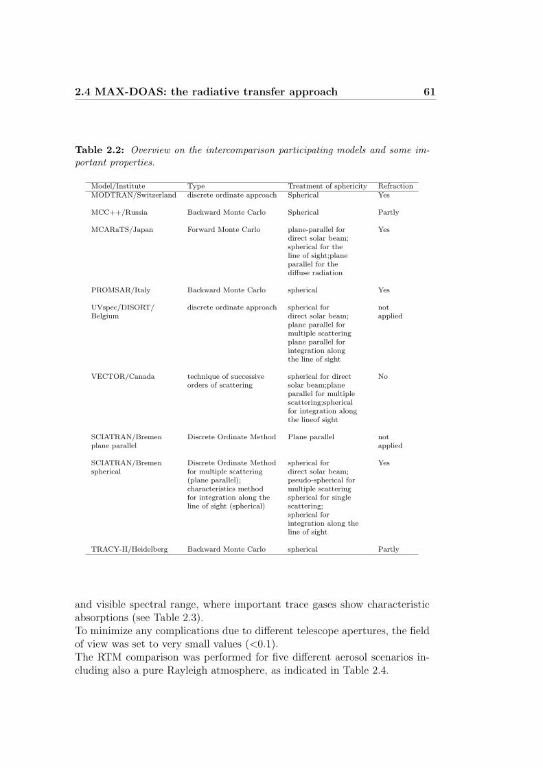
2.4 MAX-DOAS: the radiative transfer approach 61
Table 2.2: Overview on the intercomparison participating models and some im-portant properties.
Model/Institute Type Treatment of sphericity RefractionMODTRAN/Switzerland discrete ordinate approach Spherical Yes
MCC++/Russia Backward Monte Carlo Spherical Partly
MCARaTS/Japan Forward Monte Carlo plane-parallel for Yesdirect solar beam;spherical for theline of sight;planeparallel for thediffuse radiation
PROMSAR/Italy Backward Monte Carlo spherical Yes
UVspec/DISORT/ discrete ordinate approach spherical for notBelgium direct solar beam; applied
plane parallel formultiple scatteringplane parallel forintegration alongthe line of sight
VECTOR/Canada technique of successive spherical for direct Noorders of scattering solar beam;plane
parallel for multiplescattering;sphericalfor integration alongthe lineof sight
SCIATRAN/Bremen Discrete Ordinate Method Plane parallel notplane parallel applied
SCIATRAN/Bremen Discrete Ordinate Method spherical for Yesspherical for multiple scattering direct solar beam;
(plane parallel); pseudo-spherical forcharacteristics method multiple scatteringfor integration along the spherical for singleline of sight (spherical) scattering;
spherical forintegration along theline of sight
TRACY-II/Heidelberg Backward Monte Carlo spherical Partly
and visible spectral range, where important trace gases show characteristicabsorptions (see Table 2.3).To minimize any complications due to different telescope apertures, the fieldof view was set to very small values (<0.1).The RTM comparison was performed for five different aerosol scenarios in-cluding also a pure Rayleigh atmosphere, as indicated in Table 2.4.
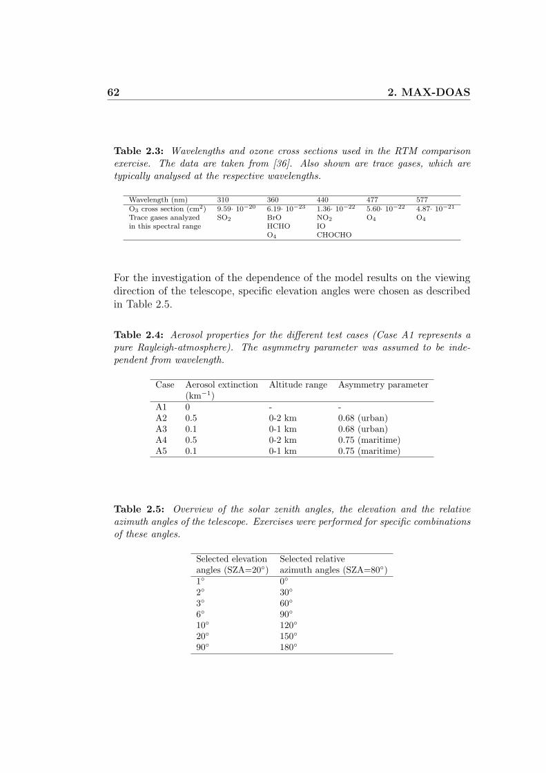
62 2. MAX-DOAS
Table 2.3: Wavelengths and ozone cross sections used in the RTM comparisonexercise. The data are taken from [36]. Also shown are trace gases, which aretypically analysed at the respective wavelengths.
Wavelength (nm) 310 360 440 477 577O3 cross section (cm2) 9.59· 10−20 6.19· 10−23 1.36· 10−22 5.60· 10−22 4.87· 10−21
Trace gases analyzed SO2 BrO NO2 O4 O4
in this spectral range HCHO IOO4 CHOCHO
For the investigation of the dependence of the model results on the viewingdirection of the telescope, specific elevation angles were chosen as describedin Table 2.5.
Table 2.4: Aerosol properties for the different test cases (Case A1 represents apure Rayleigh-atmosphere). The asymmetry parameter was assumed to be inde-pendent from wavelength.
Case Aerosol extinction Altitude range Asymmetry parameter(km−1)
A1 0 - -A2 0.5 0-2 km 0.68 (urban)A3 0.1 0-1 km 0.68 (urban)A4 0.5 0-2 km 0.75 (maritime)A5 0.1 0-1 km 0.75 (maritime)
Table 2.5: Overview of the solar zenith angles, the elevation and the relativeazimuth angles of the telescope. Exercises were performed for specific combinationsof these angles.
Selected elevation Selected relativeangles (SZA=20) azimuth angles (SZA=80)1 0
2 30
3 60
6 90
10 120
20 150
90 180

2.4 MAX-DOAS: the radiative transfer approach 63
Basic test of the model properties (exercise 0)
The first step of the RTM comparison was to check basic model results for asimple viewing geometry. This check was performed to avoid any elementarymistakes, which would later complicate the interpretation of the results forthe MAX-DOAS settings. Only Rayleigh scattering was allowed. The zenithviewing geometry was chosen and the solar zenith angle was set to 70. Thisexercise was carried out for all five wavelengths (see Table 2.3).
In Fig. 2.6 the results for the vertical optical depth (with respect toRayleigh scattering) and the normalized radiances (taking into account alsoozone absorption) are shown. Figure 2.6 shows that the optical depth in-
Figure 2.6: Modelled vertical optical depth (VOD) with respect to Rayleigh scat-tering (top) and normalised radiance taking into account also ozone absorption(bottom), as a function of wavelength.
creases with decreasing wavelength as expected for the strong wavelengthdependence of Rayleigh scattering. Accordingly, the normalized radiancesincrease towards shorter wavelengths, but decrease again for the shortestwavelength (310 nm) because of the strong ozone absorption.

64 2. MAX-DOAS
The results for the optical depth and normalized radiances are almost iden-tical for all RTMs indicating that all models treat Rayleigh scattering con-sistently.
The Box-AMFs derived from all models for zenith viewing geometry anda solar zenith angle of 70 are displayed in Fig. 2.7. For atmospheric layers at
Figure 2.7: Box-AMFs for zenith viewing geometry at a solar zenith angle of70. For low altitudes, the box-AMFs are about unity; for high altitudes about1/cos(SZA)≈2.9. Please note that the altitude is displayed on a logarithmic scale.
low altitudes, the box-AMFs are about unity, since the observed photons havetraversed these layers almost exclusively on a vertical path. In contrast, the

2.4 MAX-DOAS: the radiative transfer approach 65
direction of the photons for the highest layers is determined by the direct solarbeam (almost all scattering events occur below). Thus, the box-AMF forthese layers is similar to the geometrical approximation AMF=1/cos(SZA)∼2.9 (for SZA=70). For some wavelengths and altitudes, also values greaterthan 2.9 are derived, indicating that multiple scattered photons enhance thegeometrical light path. For the layers between the surface and 20 km, partof the photons are already scattered above, part are scattered below and thebox-AMF is between unity and 2.9. It is interesting to note that at 310 nmeven for the highest altitudes values less than 2.9 occur, indicating that asubstantial fraction of the observed photons is scattered above 20 km.
From the test of the basic model parameters it was possible to concludethat all RTMs worked with similar prerequisites. The differences in themodelled optical depths and the normalized radiances were within only a fewpercent. Also the agreement of the modelled box-AMFs from the differentmodels was good (within 5% or better) being the differences partly explainedby the way in which Earth’s sphericity is treated.
Variation of the elevation angle of the telescope (exercise 1)
The major characteristic of MAX-DOAS measurements is that the illumi-nated sky is observed under different elevation angles of the telescope. Forlow elevation angles (towards the horizon) the path length in the lowestpart of the atmosphere is significantly longer than for higher elevation an-gles (towards the zenith). Accordingly, the sensitivity for the boundary layerincreases with decreasing elevation angle. However, it must be noted thatthe sensitivity towards trace gases in the boundary layer is limited by theatmospheric visibility. In general, the visibility is decreasing towards smallerwavelengths because of the strong wavelength dependence of Rayleigh scat-tering. Moreover, especially for polluted situations, aerosol scattering furtherreduces the visibility (see also chapter 1, section 1.4); thus MAX-DOAS ob-servations are very sensitive to the atmospheric aerosol load.Within the exercise 1, aerosol scenarios A1 and A2 (see Table 2.4) were inves-tigated. The calculations were performed for 7 elevation angles between 1
and 90 (see Table 2.5). The solar zenith angle was set to 20 and the relativeazimuth angle to zero. The calculations were restricted to two wavelengths(360 nm, 577 nm) in order to minimize the computational effort.
Results for the box-AMFs are shown in Figs. 2.8 and 2.9 for the twowavelengths, respectively. As expected, the largest values are found for thesmallest elevation angles and the lowest atmospheric layers. Especially forlow extinction along the line of sight (in particular without aerosols, pureRayleigh atmosphere or scenario A1) the box-AMFs for the lowest layers be-

66 2. MAX-DOAS
come very large for 1 elevation angle (>40, the geometrical approximationfor a plane parallel atmosphere would be 1/sin(1)∼ 57). These stronglyextended absorption paths cause the high sensitivity of MAX-DOAS obser-vations for the boundary layer. For larger elevation angles, the box-AMFsfor the lowest atmospheric layers decrease monotonously. For the highestatmospheric layers, the box-AMF converges towards the geometrical approx-imation for a solar zenith angle of 20 (1/cos(20))∼ 1.06). If no aerosolsare present, the box-AMFs decrease systematically with increasing altitude,indicating that an increasing number of photons has been scattered belowthat altitude.If aerosols are present, two major changes can be observed. First, the box-AMFs for the lowest atmospheric layers become systematically smaller (thismakes MAX-DOAS observations particularly sensitive to aerosol properties).Second, multiple scattering on aerosols can cause an enhancement of the box-AMFs for atmospheric layers in and directly above the aerosol layer (0-2 km);consequently, the box-AMFs for these layers are slightly enhanced (comparedto the layers above). This effect can be best observed for high elevation an-gles, particularly for zenith direction, for which the highest box-AMFs arefound for altitudes between 1 km and 5 km (Figs. 2.8 and 2.9, bottom, right).
In general, again very good agreement (differences <5%) was found formost of the cases. Systematic differences occurred for the exercise for a pureRayleigh atmosphere and 577 nm. For these cases, the path length along theline of sight becomes very long and thus the influence of the Earth’s sphericitybecomes especially important. The line of sight of the models using planeparallel geometry stays closer at the surface for larger distances from theinstrument, causing systematically larger box-AMFs for low elevation angles.
Variation of the azimuth angle (exercise 2)
The relative azimuth angle between the direction of the telescope and thesun has an important influence on the amount of observed photons which areonly scattered once (to a lesser degree also on photons which are scatteredonly a few times). The probability of these photons to be scattered intothe telescope is directly proportional to the phase function of the scatteringprocess. For Rayleigh scattering the phase function has a symmetric maxi-mum in forward and backward direction causing a maximum in the observednormalized radiance for relative azimuth angles of 0 and 180; for a relativeazimuth angle of 90 (and 270) a minimum occurs (see chapter 1, section1.3.1 and chapter 3, section 3.3.2). For scattering on aerosols, the phase func-tion typically has a pronounced maximum in forward direction (see chapter1, section 1.3.2 and chapter 3, section 3.3.2). Thus, the observed normalized

2.4 MAX-DOAS: the radiative transfer approach 67
radiance for a relative azimuth angle of 0 is much larger than for 180.In contrast to the single scattered photons (or those with only few scat-
tering events), the contribution of multiple scattered photons depends onlyweakly on the relative azimuth angle. Thus, the strength of the azimuthdependence of the normalized radiance (and also of the box-AMF) decreasesfor an increasing fraction of multiple scattered photons (for example, insidea dense cloud, the normalized radiance does not depend on the viewing di-rection anymore).
In this exercise, box-AMFs were modelled for 7 relative azimuth angles(0, 30, 60, 90, 120, 150, 180). The elevation angle was set to 2 and thesolar zenith angle was set to 80 ensuring that the different relative azimuthangles relate to a representative range of the scattering phase functions forsingle scattered photons. The model runs were performed for a pure Rayleighatmosphere and for two aerosol scenarios (see Table 2.4).Figure 2.10 shows the box-AMFs for 360 nm as a function of altitude. Thedifferent graphs show the results for different relative azimuth angles (0,90, 180) and aerosol scenarios (pure Rayleigh atmosphere and the aerosolscenario A2). It can be noticed that, for most cases, a similar dependenceon altitude as for the first exercise is found. The highest box-AMFs (about1/ cos(2) ∼ 28) are found for the lowest atmospheric layers; with increasingaltitude they decrease to values close to the geometrical approximation fora solar zenith angle of 80 (1/ cos(80) ∼ 5.8). For the aerosol scenario A2(see Table 2.4), the box-AMFs show minimum values within the aerosol layer(0-2 km). This indicates that this layer is characterized by a high fraction ofmultiply scattered photons. The effective light paths of the diffuse radiationin these layers are smaller than the light paths in the layers below and above,which are determined by the slant line of sight and slant direct solar beam.In summary, we can again state that good agreement (differences <5%) wasfound for most of the cases between the various RTMs.

68 2. MAX-DOAS
Figure 2.8: Box-AMFs for 360 nm as a function of altitude (logarithmic scale).Left: pure Rayleigh atmosphere. Right: including also aerosol scattering (scenarioA2, see Table 2.4). From top to bottom the elevation angle increases from 1 to90.
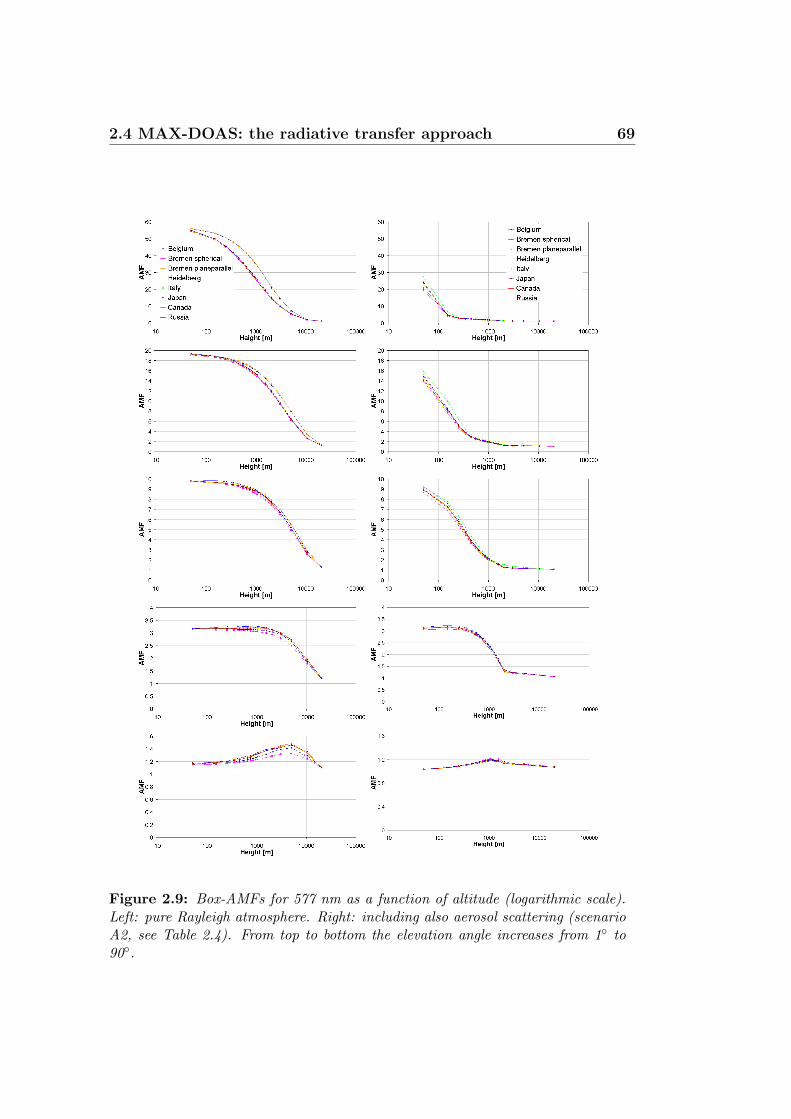
2.4 MAX-DOAS: the radiative transfer approach 69
Figure 2.9: Box-AMFs for 577 nm as a function of altitude (logarithmic scale).Left: pure Rayleigh atmosphere. Right: including also aerosol scattering (scenarioA2, see Table 2.4). From top to bottom the elevation angle increases from 1 to90.
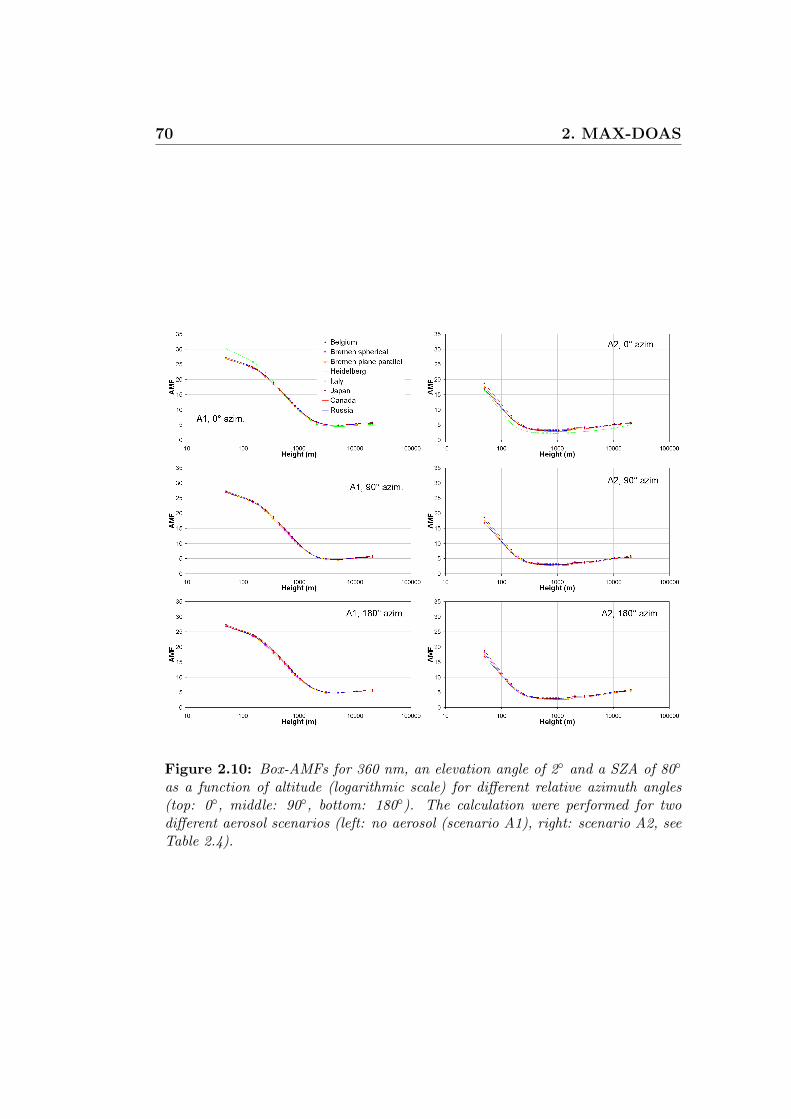
70 2. MAX-DOAS
Figure 2.10: Box-AMFs for 360 nm, an elevation angle of 2 and a SZA of 80
as a function of altitude (logarithmic scale) for different relative azimuth angles(top: 0, middle: 90, bottom: 180). The calculation were performed for twodifferent aerosol scenarios (left: no aerosol (scenario A1), right: scenario A2, seeTable 2.4).

Chapter 3
The Monte Carlo RadiativeTransfer Model PROMSAR
Propagation of light in the atmosphere can be mathematically describedby the Radiative Transfer Equation (RTE). Solutions to the RTE can beobtained both analytically (e.g., [37], [38]) and numerically (e.g. [39]).
The Monte Carlo (MC) method is a powerful numerical tool for perform-ing radiative transfer simulations, even in complex geometries and with theadvantage that it does not require extra simplifying assumptions comparedwith analytical methods.There have been many examples of MC studies of radiative transfer in scat-tering and absorbing media, e.g. [40], [41], [42].Monte Carlo methods are used extensively in problems involving optical prop-agation and atmospheric radiative transport, since the atmosphere is a nonhomogeneous medium with multiple scattering and polarization effects com-bining to make the problem extremely difficult for analytical treatment.
In this chapter, after introducing the radiometric quantities and the radia-tive transfer equation, the Monte Carlo radiative transfer model PROMSARwill be described in detail and applications to different cases discussed.
3.1 Radiometric quantities
Electromagnetic radiation may be viewed as an ensamble of waves whichtravel through a vacuum at the speed of light c = 3× 10⁸ ms−1. The wavesmay exhibit a continuous range of wavelengths, and the totality of all possiblewavelengths is called the electromagnetic spectrum. Quantum theory predictsthat energy transmitted by electromagnetic radiation exists in discrete unitscalled photons. The amount of energy associated with a photon of radiation

72 3. The PROMSAR Monte Carlo RTM
is given by hν, where ν is the frequency of the radiation, expressed in s−1 andh is the Planck’s constant, which is equal to 6.626 × 10⁻³⁴ Js. The amountof energy contained in a photon of radiation is inversely proportional to thewavelength of radiation, according to the relationship ν = c/λ.
The rate of energy transfer by electromagnetic radiation is called the ra-diant flux, which has units of energy per unit time: watts (W ). For example,the radiant flux from the sun is about 3.90 · 1026 W.By dividing the radiant flux by the area through which it passes, we obtainthe irradiance, E, which is expressed in units of Wm−2. The averaged ir-radiance of solar radiation reaching the Earth’s orbit is about 1370 Wm−2,and is called solar constant. The irradiance per unit wavelength interval atwavelength λ is called the monochromatic irradiance, Eλ, which has units ofWm−2µm−1. With this definition, the irradiance is readily seen to be:
E =
∫ ∞
0
Eλ · dλ. (3.1)
Thus, if Eλ is plotted as a function of λ as in Fig. 3.1, the area under thecurve between any two wavelengths is proportional to the contribution of theradiation in that wavelength band to the total irradiance. The irradiance
Figure 3.1: Emission spectra for blackbodies with different temperatures. From[4].
impinging onto the Earth’s atmosphere can be measured using instrumentslocated on high mountains, such as the Kitt Peak1, or using satellite-mounted
1The Kitt Peak National Observatory (KPNO) is a United States astronomical ob-servatory located on a 2.096 km peak of the Quinlan Mountains in the Arizona-SonoranDesert on the Tohono O’odham Nation, 88 km southwest of Tucson. With 23 telescopes,it is the largest, most diverse gathering of astronomical instruments in the world.

3.1 Radiometric quantities 73
sensors. An example for a spectrum measured with satellite-mounted sensorsis the “Wehrli spectrum” [43], and is shown in Fig. 3.2.If we want to identify the part of the irradiance that is coming from directionswithin some specified infinitesimal arc of solid angle dω, it is useful to definethe radiance, L, which is the irradiance per unit solid angle, expressed inWm−2sr−1. Given the radiance, the irradiance can be expressed as:
Figure 3.2: The extraterrestrial solar irradiance by Wehrli [43].
E =
∫ 2π
0
L · cosφ · dω (3.2)
where the zenith angle φ is the angle between the direction of the radiationand the normal to the surface in question. The quantity L · cosφ is thereforethe component of the radiance normal to the surface. Equation 3.2 statesthat the irradiance represents the combined effects of the normal componentof the radiation coming from the whole hemisphere. An element of the solidangle dω can be expressed in spherical coordinates in the form
dω = sinφ · dφ · dθ, (3.3)
where θ is the azimuth angle. The integral of dω over the upper hemisphereis given by:∫ π
2
0
sinφ · dφ∫ 2π
0
dθ = 2π, (3.4)

74 3. The PROMSAR Monte Carlo RTM
which is readily seen to be equal to half the area of the sphere of unit radius.Using the definition of solid angle, Eq. 3.2 can be written in the form
E =
∫ 2π
0
∫ π2
0
L · cosφ · sinφ · dφ · dθ. (3.5)
3.2 Radiative transfer equation
The radiative transfer equation gives the change in radiance along a beam ofelectromagnetic energy at a point in the atmosphere. The processes affectingradiation along a beam are scattering of radiation out of the beam, absorptionof radiation along the beam, multiple scattering of indirect, diffuse radiationinto the beam, single scattering of direct, solar radiation into the beam, andemission of infrared radiation into the beam. Single scattering occurs when aphoton of radiation is redirected into a beam after it collides with a particleor gas molecule, as shown in Fig. 3.3. Multiple scattering occurs when aphoton enters a beam after colliding sequentially with several particles orgas molecules, each of which redirects the photon. Solar radiation that hasnot yet been scattered is direct radiation. Radiation, either solar or infrared,that has been scattered is diffuse radiation.
Figure 3.3: Single scattering of direct solar radiation and multiple scattering ofdiffuse radiation adds to the intensity along a beam of orientation (µ, θ). Adaptedfrom [11].
Assuming that the atmosphere can be represented by a horizontally strat-ified medium (plane-parallel approximation), the radiative transfer equationcan be expressed by:
µ · dLλ
dz= −kλ(z) · [Lλ(z;µ, θ)− Jλ(z;µ, θ)] (3.6)
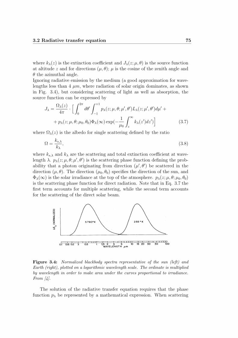
3.2 Radiative transfer equation 75
where kλ(z) is the extinction coefficient and Jλ(z;µ, θ) is the source functionat altitude z and for directions (µ, θ); µ is the cosine of the zenith angle andθ the azimuthal angle.Ignoring radiative emission by the medium (a good approximation for wave-lengths less than 4 µm, where radiation of solar origin dominates, as shownin Fig. 3.4), but considering scattering of light as well as absorption, thesource function can be expressed by
Jλ =Ωλ(z)
4π·[ ∫ 2π
0
dθ′∫ +1
−1
pλ(z;µ, θ;µ′, θ′)Lλ(z;µ
′, θ′)dµ′ +
+ pλ(z;µ, θ;µ0, θ0)Φλ(∞) exp(− 1
µ0
∫ ∞
z
kλ(z′)dz′)
](3.7)
where Ωλ(z) is the albedo for single scattering defined by the ratio
Ω =ks,λ
kλ
, (3.8)
where ks,λ and kλ are the scattering and total extinction coefficient at wave-length λ. pλ(z;µ, θ;µ
′, θ′) is the scattering phase function defining the prob-ability that a photon originating from direction (µ′, θ′) be scattered in thedirection (µ, θ). The direction (µ0, θ0) specifies the direction of the sun, andΦλ(∞) is the solar irradiance at the top of the atmosphere. pλ(z;µ, θ;µ0, θ0)is the scattering phase function for direct radiation. Note that in Eq. 3.7 thefirst term accounts for multiple scattering, while the second term accountsfor the scattering of the direct solar beam.
Figure 3.4: Normalized blackbody spectra representative of the sun (left) andEarth (right), plotted on a logarithmic wavelength scale. The ordinate is multipliedby wavelength in order to make area under the curves proportional to irradiance.From [4].
The solution of the radiative transfer equation requires that the phasefunction pλ be represented by a mathematical expression. When scattering

76 3. The PROMSAR Monte Carlo RTM
is due only to air molecules, the phase function is provided by the Rayleightheory. In other cases (e.g. when solid and liquid particles contribute to thescattering of light), the phase function can be derived from the Mie theory,if the physical and chemical characteristics of the particles are known. Adetailed analysis of the Rayleigh and Mie phase functions will be given insection 3.3.2.When particle scattering is included in the radiative transfer equation, an-alytical solutions become difficult to obtain and numerical solutions areneeded. The Monte Carlo method is a powerful numerical tool for performingradiative transfer simulations including also multiple scattering with variousphase functions involved. The Monte Carlo approach to the radiative transferequation will be described in the following section.
3.2.1 The Monte Carlo approach to the RTE
The Monte Carlo method is defined as representing the solutionof a problem as a parameter of a hypothetical population, andusing a random sequence of numbers to construct a sample ofthe population, from which statistical estimates of the parametercan be obtained.Halton, 1970 [44]
The Monte Carlo approach to atmospheric radiative transfer consists of us-ing probabilistic concepts and methods to simulate the trajectories of eachindividual photon, which is subject to random events. Though the attenu-ation of a light beam obeys a well known exponential function, in fact, thecollision of a single photon with a scattering center can happen at the verybeginning or at the very end of a given distance to cover and, moreover, atthe scattering site the photon can be scattered into any direction. Theseprocesses can be classified as random processes.
The basis of MC is that every interaction of a photon in the atmospherecan be described via a Probability Density Function (pdf), the integral ofwhich (the Cumulative Distribution Function, cdf) can be linked to a randomnumber, R. The probability for the photon to get scattered on its way toa given point is known. So a random number can be used to decide aboutthis. At the scattering site, the photon can be scattered into any direction,the probability of a scattering being governed by the correspondent phasefunction. Here a random number can be used to decide which direction thisindividual photon gets scattered into. Once the probability of one event isknown, it is possible to calculate the probability of a sequence of events as a

3.2 Radiative transfer equation 77
Markov chain2, because the events are independent. By generating enoughrandom realizations, the physical process (the radiation transport) can besimulated in a statistical sense.
The statistical basis
In this section we will define some basic statistical terms to lay a formalfoundation for the validity of Monte Carlo calculations. At least in formalsense, all Monte Carlo calculations can be considered as the evaluation of anumber of integrals of the type
〈k〉 =
∫P (x)k(x)dx (3.9)
where the random variable k(x) is distributed according to the probabilitydensity function P (x), and 〈k〉 specifies a certain numerical property of k(x).Estimates of 〈k〉 can be obtained by sampling a great enough number ofrandom variables x from P (x) and averaging the correspondent k(x) values.It is also convenient to consider the variance of k defined
var(k) ≡∫P (x)(k(x)− 〈k〉)2dx =
∫P (x)k2(x)dx− 〈k〉2. (3.10)
In the Monte Carlo simulation of radiation transport, the random variablek(x) specifies a unique track, the distribution function P (x) gives the prob-ability of occurrence of this particular track and the function 〈k〉 refers to acertain numerical property of the track (the expectation). The simulation ofa track provides a random value xi of x so that the value of k(xi) is obtainedduring the simulation of each track and accumulated in a counter. Aftergenerating a large number N of random tracks, Monte Carlo estimators of〈k〉 and var(k) are evaluated, respectively, as
k =1
N
N∑i=1
k(xi) (3.11)
and
s2(k) =1
N
N∑i=1
k2(xi)− [1
N
N∑i=1
k(xi)]2. (3.12)
2A Markov chain, named after Andrey Markov (1856-1922), is a discrete-time stochasticprocess with the property that, given the present state, future states are independent ofthe past states.

78 3. The PROMSAR Monte Carlo RTM
It is important to note here that the evaluation of s2(k) requires scoring ofnot only k(xi) but also the squared contributions k2(xi).Actually, a Monte Carlo simulation can be thought of as a “computer ex-periment” planned to measure 〈k〉, which yields the outcome k. As in anyreal experiment, if we repeat it a number of times (with different seeds ofthe random number generator, to make the experiment “independent”) weobtain different results. These fluctuate about the mean
〈k〉 = 〈 1
N
N∑i=1
k(xi)〉 =1
N
N∑i=1
〈k〉 = 〈k〉 (3.13)
with variance
s2(k) = var[1
N
N∑i=1
k(xi)] =1
N2
N∑i=1
var(k) =1
Nvar(k) (3.14)
where use have been made of properties of the expectation and variance op-erators.From the central limit theorem, it follows that, in the limit N → ∞, theprobability distribution of k is a normal (Gaussian) distribution. The quan-tity
s2(k) ≡ s2(k)
N=
1
N 1
N
N∑i=1
k2(xi)− [1
N
N∑i=1
k(xi)]2. (3.15)
in the limit N →∞, is an unbiased estimator 3 for var(k). Simulation resultsshould always be expressed in the form k±n·s(k). With n = 3 the probabilitythat the “true value” 〈k〉 lies within the error bar is approximately 0.997.
3An estimator, θ, can be defined as a useful approximation to a quantity of interest, Q,which may be derived from a Monte Carlo calculation. This means that θ is not expectedto fluctuate far from Q. Formally,
〈(θ −Q)2〉Q2
1. (3.16)
Acceptable values of the ratio depend on the application. We write
〈(θ −Q)2〉 = 〈(θ − 〈θ〉)2〉+ (〈θ〉 −Q)2 (3.17)
and observe that the quality of θ as a measure of Q comes separately from the varianceof θ and from the departure of its mean from Q. The quantity 〈θ〉 −Q is called the biasof the estimator. An unbiased estimator is one for which 〈θ〉 = Q, and the mean value ofany experiment is just Q whatever the number N may be.

3.3 Description of the PROMSAR RTM 79
In practical calculations it may happen that, after a relatively long sim-ulation time, the quantity of interest still has a large statistical uncertaintys(k) that makes the numerical result meaningless. The quantity var(k) is anintrinsic property of the function k(x) and, for a sufficiently large number Nof generated tracks, its estimator s2(k) is independent of N . Consequently,s(k) is roughly proportional to N−1/2, for large N . Thus, the obvious methodto reduce the variance is simply to increase the number of generated tracks.However, as the simulation time is roughly proportional to N , in order to ob-tain a reduction of the statistical uncertainty by a factor of, say, 10 we mustincrease the computer time by a factor of 100. The aim of the so called vari-ance reducing techniques (VRTs) is to yield results that are more accuratethan those of the analogue simulation, without increasing the computationtime. A practically oriented review of variance reducing methods in radiationtransport has been given in [45].
Normally, variance reducing methods are based on transformations that,with the same calculation effort (computer time), reduce the variance of thequantity of interest to a fraction of its original value. These transformationsusually involve additional calculations which consume some extra time andmust be kept below reasonable limits. As a figure of merit to evaluate theeffectiveness of a variance reducing method, it is common to use the efficiencyε, defined as
ε =1
s2(k) · T ·(3.18)
where T is the computer time spent in the simulation. As s2(k) and T areproportional to N−1 and N respectively, ε is independent of N .
3.3 Description of the PROMSAR RTM
PROMSAR (PROcessing of Multi-Scattered Atmospheric Radiation) is abackward Monte Carlo model in which simulation of the radiative transfer inthe atmosphere is performed according to the physical and geometrical dataof an assigned atmospheric system.Many experiments with independent radiation source and receiving opticaldevice are allowed to be simulated by the PROMSAR code, including forexample lidar experiment simulations which, however, will not be discussedin this thesis. The main computed quantities important for the study pre-sented here refer to optical depths and transmittances of the atmosphere,direct and diffuse radiation contributions to the global radiation reaching thelowest boundary surface of a given environment, and radiance calculations

80 3. The PROMSAR Monte Carlo RTM
(including air mass factors for target species) for a detector with assignedcentral coordinates, diameter, direction cosines of the normal to the detectorsurface, line of sight and field of view. The detector can be placed at ground,as well as on board an aicraft or on satellite platforms.The radiation source foreseen by the code is a monochromatic radiation inthe ultraviolet-infrared range. Since the wavelength region of interest forDOAS applications is the UV/visible region, results reported in this thesisrefer to this wavelength range.
3.3.1 Backward Monte Carlo technique
The strict Monte Carlo experiment is to “fire” photons out of a radiationsource along initial directions governed by the aperture of that source. Thenrandom numbers govern the entry of the photons into a model atmosphere,where they are scattered, by which scatterer, and in which direction. Thephotons direction is accordingly altered at each scattering location. In theirrandom walk, eventually the photons will be absorbed, or either leave theatmosphere or reach the altitude where the modelled detector is located.There, the impact location and the incident angle are compared to the de-tector specifications. Each radiative transfer process can be modelled andreproduced with accuracy, and no approximations are needed. The absorp-tion would be modelled by the destruction of the photon and the abort ofthe path calculation.The problem in this is that the detector must reproduce realistic dimensionsand aperture angle, i.e., the photon not only must reach the detector alti-tude, but must actually hit the detector, and do so from a solid angle definedby the line of sight and the aperture angle. This results in a very low totalprobability for one single photon to get “recorded” by the instrument.
An effective solution to this problem comes from the following consider-ations: the probability for a photon to leave the source (defined itself by itsarea and aperture angle) and reach a detector under the required conditionsis the same as the probability that the photon leaves the detector on the wayit entered it and reaches the source, i.e., follows backward the path it hasin fact covered in forward direction. This is feasible, since any transmissionprobability (the probability that a photon covers the distance d from onegiven point to another) and any scattering probability (for a given scatteringangle θ to occur) are the same in both directions. This approach is called“backward Monte Carlo”.Therefore, with the backward approach, each starting photon emerges fromthe detector in the line of sight direction and is traced backward since it leavesthe atmosphere in the sun direction (or is absorbed). As demonstrated by

3.3 Description of the PROMSAR RTM 81
Collins [46], the backward Monte Carlo approach should be used to efficientlysimulate narrow field of view instruments. It moreover eliminates a numberof other problems involved in the forward Monte Carlo scheme (see also [47]).
3.3.2 The photon history tracking
A photon is emitted, it travels a distance, and then somethinghappens to it.
A unitary weight is assigned to each photon emerging from the point wherethe intensity (or radiance) is to be computed with a direction opposite tothat in which the photon would phisically propagate. Changes in the photonweight during the simulation of its history is the signature of scattering, ab-sorption and reflection contributions to the variation of the source intensity.Photon paths and interactions are simulated by sampling randomly from thevarious pdf ′s that determine the interaction lengths of each step in the ran-dom walk, scattering angles, and absorption rates.For that purpose, the first step is sampling pseudo-random numbers4 uni-formly distributed in the interval [0,1]. As regard the random number gen-eration, two algorithms are foreseen by the PROMSAR code: the first onegenerates the first random number of each history, while the second one, onthe basis of this random number, generates the random numbers inside thehistory. In this way, corresponding histories in independent calculations be-gin with the same random number.Second, the source parameters, photon paths and scattering angles are sam-pled according to the appropriate pdf ′s. To sample a quantity x0 from aprobability distribution function P (x), which is normalized over all x, thefollowing equation has to been solved:
R =
∫ x0
a
P (x)dx = ψ(x0) (3.19)
where R is a random number sampled uniformly from the range 0 to 1, a isthe lower limit of the range over which x is defined and ψ is the cumulativedistribution function5.
4pseudo-random numbers are generated according to a strict mathematical formula andtherefore reproducible and not at all random in the mathematical sense but are supposedto be indistinguishable from a sequence generated truly random.
5For every real number x, the cdf of X is given by
x −→ FX(x) = P (X ≤ x), (3.20)
where the right-hand side represents the probability that a random variable X takes on a
82 3. The PROMSAR Monte Carlo RTM
We need to sample how far a photon travels before being absorbed orscattered. The probability that a photon travels an optical path (OP ) with-out an interaction is e−OP . The probability of scattering prior to OP is1− e−OP = ψ(OP ). Therefore we can sample from the cdf according to
R =
∫ OP
0
e−xdx (3.21)
giving
OP = − ln(1−R) = − ln(R) (3.22)
where R is a random number sampled uniformly from the range 0 to 1.To avoid the photon escaping the atmosphere without interaction with itscomponents, we can force the photon to scatter at least once. The so calledforced collision technique allows the physical system to be better explored bythe travelling photon, by increasing the collision number. This technique isusefully used when, notwithstanding small optical thickness, collision eventsare of special interest in the simulation. At each point of emission/collisionwe calculate the optical depth to the edge of the atmospheric grid, Dleak. Theuncolliding and colliding probabilities are exp(−Dleak) and [1−exp(−Dleak)],respectively, giving rise to the two corresponding particle weight fractionswhich separately contribute to the leakage and collision analytical estimates.The colliding fraction will remain in the system giving rise to a next collisionpoint according to the distribution low (truncated exponential distribution[46]):
e−x
1− e−Dleak. (3.23)
Equation 3.21 becomes
R =
∫ OP
0
e−x
1− e−Dleakdx (3.24)
from which the following expression for the optical distance to collision isderived:
OP = − ln[1−R · (1− e−Dleak)]. (3.25)
value less than or equal to x. The probability that X lies in the interval (a,b] is thereforeFX(b)− FX(a) if a < b.

3.3 Description of the PROMSAR RTM 83
where R is a random number sampled uniformly from the range 0 to 1. Whenthe collision is forced to occur, the photon statistical weight before collision,wn−1, is adjusted to remove the bias introduced by forcing the collision:
wn = wn−1[1− e−Dleak ]. (3.26)
Since the force collision technique is time consuming and can greatly andirregularly affect the particle weight, option is left to the user to force onlythe first collision (or first few collisions), the remaining ones being left tochance as usual, according to an analogue simulation.Forced collisions are not allowed for those lines of flight hitting reflectingsurfaces, in order not to prevent the photon from undergoing reflection. Inthis case, the distance to collision is sampled according to Eq. 3.22. If areflection actually occurs, a Lambert refection law (i.e. cosine distributionalong the normal to the surface) is considered. The photon weight is conse-quently decreased by the surface albedo coefficient. Absorbed radiation atthe surface is analytically estimated by means of the same law.
At each collision point the photon’s fate is determined by the probabil-ity that the photon is scattered or absorbed. The statistical weight of the“survived” photon is so multiplied to the so called single scattering albedo,defined as
ω =sc
ac+ sc(3.27)
where ac and sc are the absorption and the scattering coefficients of thelayer to which the scattering point belongs, respectively. The correspondingweight fraction absorbed
1− sc
ac+ sc(3.28)
gives rise to the expected value of absorption at each collision point along thephoton’s path (collision estimator for absorption). In addition, an estimateof the absorption can also be done by means of the more effective distanceestimator, i.e., through the computation of the product between the photonpath length before collision and the absorption coefficient along that path.
Having sampled a random optical depth OP we may then calculate, onthe basis of the total macroscopic cross section of the layer to which thepoint scattering belongs, the pysical distance L that the photon travels beforeundergoing interaction. The photon’s position is then updated according to:
x = x+ L sin θ cosφ, y = y + L sin θ sinφ, z = z + L cos θ (3.29)

84 3. The PROMSAR Monte Carlo RTM
where θ and φ are, respectively, the scattering and azimuth angles of themotion direction before collision.
A random number R is then generated to decide the type of scatteringevent, i.e., molecular or aerosol scattering. The phase function of the respec-tive scatterer is used to derive the new motion direction of the photon. Asalready introduced in section 3.2, the phase function, f(cos θ), describes theangular distribution of scattered light. It has no physical dimension, and itsintegral over all directions is 1:∫ 2π
0
∫ π
0
f(cos θ)
4πdθdφ = 1. (3.30)
Rayleigh scattering
The angular distribution of scattered light by the air molecules and particlesmuch smaller than the incident wavelength (see also chapter 1, section 1.3.1)is described by the Rayleigh scattering phase function
f(cos θ) =3
16π· 2
(2 + δ)· [(1 + δ) + (1− δ) · cos2 θ] (3.31)
where δ is the depolarization factor that gives the correction for the depolar-ization effect of scattering from anisotropic molecules. When δ goes to zero,that is, no depolarization or symmetric molecules, Eq. 3.31 reduces to
f(cos θ) =3
16π· [1 + cos2 θ] (3.32)
which is a commonly used approximation for the Rayleigh phase function. Avalue of δ = 0.0295 is generally used [48], so that Eq. 3.31 becomes:
f(cos θ) = 0.0605 + 0.05722 cos2 θ. (3.33)
A graphic representation of Eq. 3.33 is given in Fig. 3.5. The Rayleigh phasefunction is symmetric around cos θ = 0 (θ = 90, θ = 180) and its valuesvary within a very restricted range.
During the photon history tracking, the time needed for selecting thescattering angle θ should be reduced as much as possible. In case of Rayleighscattering this can be successfully achieved carrying out random accessesto precomputed cosine probability tables. An example is given by Table3.1. The first column contains (n+ 1) ci values (0, 1/n, 2/n, 3/n, ..., 1) whichcan be obtained by dividing the range [0,1] into n intervals (in this case

3.3 Description of the PROMSAR RTM 85
Figure 3.5: Rayleigh phase function according to Eq. 3.33.
n = 32); the second column contains (n + 1) cos θi values, in the range [-1,+1], corresponding to ci values6. The advantage of using such a table isthat, when a scattering event occurs during the photon history tracking, arandom number c between [0,1] is sampled (which will be comprised in oneof the intervals [ci, ci+1]) and the correspondent cosine angle cos θ is quicklydetermined through simple linear interpolation between cos θi and cos θi+1.In order to verify if the correspondence between ci and cos θi defined inTable 3.1 is correct, we reproduce the Rayleigh phase function by means ofa Monte Carlo procedure and compare the numerical values obtained withthe analytical ones7. The checking procedure is summarized in Fig. 3.6 andin Table 3.2. Figures 3.6 a) and b) show, respectively, the histogram withthe number of counts per interval and the normalized histogram, that is, theMonte Carlo Rayleigh phase function. Figure 3.6 c) shows the numerical(MC) and analytical values of the Rayleigh phase function computed forthe central point of each cosine interval. The values of the numerically- andanalitically- computed Rayleigh phase function have been compared in Table3.2.
6In order to build such a table we consider a great number M of cosine values andcalculate the respective cdf ′s so as to define a correspondence between a value in the range[-1,+1] (the cosine) and a value in the range [0,1] (the cdf). Taking into account that eachci value in Table 3.1 falls into one of the M intervals [cdfm,cdfm+1], the correspondentcos θi value in Table 3.1 is easily computed by linear interpolation.
7The MC procedure starts dividing the cosine range [-1,+1] in an arbitrary number m ofinterval, e.g. 16 intervals. Each cos θi value of Table 3.1 falls into one of these m intervals.If a high number of cos θi values is generated (e.g. 106), the normalized number of countsinto each mth interval supplies a numerical estimate of the Rayleigh phase function.

86 3. The PROMSAR Monte Carlo RTM
Table 3.1: Cosine probability table for Rayleigh scattering.
ci cos θi
0 -10.03125 -0.95690.0625 -0.91190.09375 -0.86480.125 -0.81550.15625 -0.76380.1875 -0.70950.21875 -0.65240.25 -0.59220.28125 -0.52890.3125 -0.46220.34375 -0.39210.375 -0.31870.40625 -0.24220.4375 -0.16310.46875 -0.08210.5 -0.00010.53125 0.0820.5625 0.1630.59375 0.24210.625 0.31860.65625 0.3920.6875 0.46210.71875 0.52880.75 0.59220.78125 0.65230.8125 0.70950.84375 0.76380.875 0.81550.90625 0.86480.9375 0.91190.96875 0.95691 1
Mie scattering
As for the Mie phase function, it must be carefully taken into account inthe simulation process the possible strong anisotropy of a scattering eventaccording to the size parameter 2πr/λ, where r is the particle radius and λthe wavelength of radiation (see also chapter 1), and the complex refractionindex n = m− iq (where q = kaλ/4π, ka being the absorption cross section).The strong anisotropy, in particular, prevents this phase function from be-
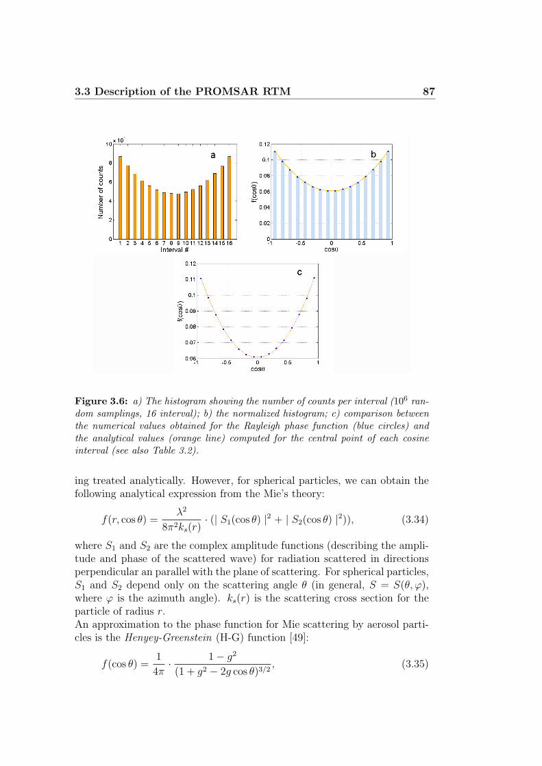
3.3 Description of the PROMSAR RTM 87
Figure 3.6: a) The histogram showing the number of counts per interval (106 ran-dom samplings, 16 interval); b) the normalized histogram; c) comparison betweenthe numerical values obtained for the Rayleigh phase function (blue circles) andthe analytical values (orange line) computed for the central point of each cosineinterval (see also Table 3.2).
ing treated analytically. However, for spherical particles, we can obtain thefollowing analytical expression from the Mie’s theory:
f(r, cos θ) =λ2
8π2ks(r)· (| S1(cos θ) |2 + | S2(cos θ) |2)), (3.34)
where S1 and S2 are the complex amplitude functions (describing the ampli-tude and phase of the scattered wave) for radiation scattered in directionsperpendicular an parallel with the plane of scattering. For spherical particles,S1 and S2 depend only on the scattering angle θ (in general, S = S(θ, ϕ),where ϕ is the azimuth angle). ks(r) is the scattering cross section for theparticle of radius r.An approximation to the phase function for Mie scattering by aerosol parti-cles is the Henyey-Greenstein (H-G) function [49]:
f(cos θ) =1
4π· 1− g2
(1 + g2 − 2g cos θ)3/2, (3.35)

88 3. The PROMSAR Monte Carlo RTM
Table 3.2: For the central point of each cosine interval, the numerical (MonteCarlo) and analytical values of the Rayleigh phase function, and their standarddeviation are shown. See also Fig. 3.6 c.
I COS ANALYTIC MC STD1 -0.9375 0.111 0.111 7.20E-052 -0.8125 0.098 0.098 6.40E-053 -0.6875 0.088 0.087 5.67E-054 -0.5625 0.079 0.078 5.13E-055 -0.4375 0.071 0.072 4.68E-056 -0.3125 0.066 0.066 4.30E-057 -0.1875 0.062 0.062 4.09E-058 -0.0625 0.061 0.061 3.99E-059 0.0625 0.061 0.061 3.99E-0510 0.1875 0.063 0.063 4.13E-0511 0.3125 0.066 0.066 4.31E-0512 0.4375 0.071 0.071 4.63E-0513 0.5625 0.079 0.079 5.17E-0514 0.6875 0.088 0.088 5.67E-0515 0.8125 0.098 0.099 6.36E-0516 0.9375 0.111 0.111 7.22E-05
where θ is the scattering angle and g is the asymmetry parameter. Eq. 3.35is valid primarily for scattering that is not strongly peaked in the forwarddirection [50], and requires advance knowledge of the asymmetry parameter.The asymmetry parameter, or first moment of the phase function, is a pa-rameter derived from the phase function itself that gives the relative directionof scattering by particles (or gases). Its analytical form is:
g =
∫ ∫4π
f(cos θ) cos θdΩ. (3.36)
The asymmetry parameter gives a measure of the asymmetry of the angularscattering. It approaches +1 for scattering strongly peaked in the forwarddirection and −1 for scattering strongly peaked in the backward direction.If g = 0, scattering is isotropic or symmetric (e.g. Rayleigh) type.
Properly tabulated aerosol phase functions or, alternatively, g values asa function of the scattering angle are achieved and processed by the PROM-SAR code8. Through integration, from the tabulated phase function (or g)values the cumulative density functions can be obtained, each one relative
8One possibility, not the only one, is to use the standard aerosol phase functions orthe g values stored in the MODTRAN (MODerate resolution TRANsmittance) code [48],[51].

3.3 Description of the PROMSAR RTM 89
to a scattering angle. During the photon history tracking, when an aerosolscattering occurs, the cdf can be compared to a random number to decidefor the corresponding scattering angle. On the analogy of Fig. 3.6 and Table3.2, Fig. 3.7 and Table 3.3 summarize the comparison between one possibleaerosol phase function (representative of an urban extinction at 440 nm) andits MC estimate.
Figure 3.7: a)The histogram showing the number of counts per interval (106 ran-dom samplings, 16 interval); b) the normalized histogram; c) comparison betweenthe numerical values obtained for the Mie phase function (blue circles) and the an-alytical values (orange line) computed for the central point of each cosine interval(see also Table 3.3).
Air mass factor calculation
At each collision point, the contribution to the intensity given by the ith scat-tering of the solar radiation by the nth photon and collected by the telescopeis given by
Intin = S · win · e−ODSun · p(θSun). (3.37)

90 3. The PROMSAR Monte Carlo RTM
Table 3.3: For the central point of each cosine interval, the numerical (MonteCarlo) and analytical values of the Mie phase function, and their standard devia-tion are shown. See also Fig. 3.7 c.
I COS ANALYTIC MC STD1 -0.9375 0.018 0.019 3.44E-052 -0.8125 0.016 0.016 3.19E-053 -0.6875 0.014 0.014 2.97E-054 -0.5625 0.014 0.014 3.08E-055 -0.4375 0.015 0.015 3.10E-056 -0.3125 0.016 0.017 3.41E-057 -0.1875 0.018 0.018 3.62E-058 -0.0625 0.021 0.020 3.72E-059 0.0625 0.026 0.027 4.12E-0510 0.1875 0.033 0.034 5.00E-0511 0.3125 0.044 0.045 5.79E-0512 0.4375 0.061 0.060 6.32E-0513 0.5625 0.089 0.090 7.83E-0514 0.6875 0.137 0.138 1.00E-0415 0.8125 0.224 0.227 1.33E-0416 0.9375 0.475 0.519 2.12E-04
ODSun is the optical depth measured from the current position of the photonto the upper boundary of the medium in the direction of propagation of theincident flux, S is equal to the incident intensity, wi
n is the weight attached tothe nth photon after the ith scattering. p(θSun) is the phase function, whichrepresents the probability density function for scattering of the photon inthe direction antiparallel to that of solar rays, being θSun the angle betweenthe direction of incidence of the photon and the direction of the solar fluxtoward the top of the atmosphere. e−ODSun represents the probability that thephoton propagates without undergoing any other collision from the currentposition to the point of incidence of the solar rays in the upper boundary ofthe atmosphere.
According to the air mass factor definition given in chapter 2 (Eq. 2.5),the ratio of the slant column density of an atmospheric absorber to its ver-tical column density has to be calculated. For this purpose the followingcomputation steps must be performed in the PROMSAR code:
1. the radiances I(λ, σ) and I(λ, 0) are calculated. Two simulations areso performed: the first one where the absorber is included (I(λ, σ)) andthe second one where the absorber is not included (I(λ, 0));
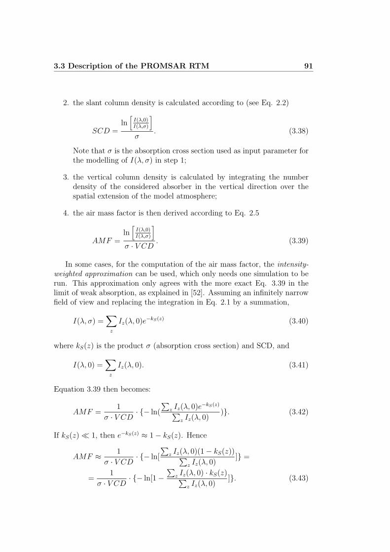
3.3 Description of the PROMSAR RTM 91
2. the slant column density is calculated according to (see Eq. 2.2)
SCD =ln
[I(λ,0)I(λ,σ)
]σ
. (3.38)
Note that σ is the absorption cross section used as input parameter forthe modelling of I(λ, σ) in step 1;
3. the vertical column density is calculated by integrating the numberdensity of the considered absorber in the vertical direction over thespatial extension of the model atmosphere;
4. the air mass factor is then derived according to Eq. 2.5
AMF =ln
[I(λ,0)I(λ,σ)
]σ · V CD
. (3.39)
In some cases, for the computation of the air mass factor, the intensity-weighted approximation can be used, which only needs one simulation to berun. This approximation only agrees with the more exact Eq. 3.39 in thelimit of weak absorption, as explained in [52]. Assuming an infinitely narrowfield of view and replacing the integration in Eq. 2.1 by a summation,
I(λ, σ) =∑
z
Iz(λ, 0)e−kS(z) (3.40)
where kS(z) is the product σ (absorption cross section) and SCD, and
I(λ, 0) =∑
z
Iz(λ, 0). (3.41)
Equation 3.39 then becomes:
AMF =1
σ · V CD· − ln(
∑z Iz(λ, 0)e−kS(z)∑
z Iz(λ, 0)). (3.42)
If kS(z) 1, then e−kS(z) ≈ 1− kS(z). Hence
AMF ≈ 1
σ · V CD· − ln[
∑z Iz(λ, 0)(1− kS(z))∑
z Iz(λ, 0)] =
=1
σ · V CD· − ln[1−
∑z Iz(λ, 0) · kS(z)∑
z Iz(λ, 0)]. (3.43)

92 3. The PROMSAR Monte Carlo RTM
If kS(z) 1, thenP
z Iz(λ,0)·kS(z)Pz Iz(λ,0)
1, and since ln(1 + x) ≈ x when x 1
AMF ≈ 1
σ · V CD·∑
z Iz(λ, 0) · kS(z)∑z Iz(λ, 0)
. (3.44)
In the case of weak absorption, then Iz(λ, σ) ≈ Iz(λ, 0) so that
AMF ≈ 1
σ · V CD·∑
z Iz(λ, σ) · kS(z)∑z Iz(λ, σ)
. (3.45)
This equation takes the weighted average of the AMFs of each ray in thecalculation, the weights being set equal to the intensity received by the in-strument for each ray.
End of history
After each collision, a new path length before the next interaction is gener-ated. This process continues until the photon has undergone a fixed numberof collisions or its weight is decreased below a preassigned threshold value(10−6 is generally used).
Besides using this criterion, other techniques can be used in the PROM-SAR code to determine the photon end of history. In particular, expectedvalues estimates are performed for absorption and leakage events.As for absorption, at each collision point option is left to the user to performan analog test on the survival probability when the photon weight falls belowan assigned threshold weight, analytically evaluating the absorption contri-bution to the statistics. As for the leakage from the atmospheric system, theuncolliding probability for lines of flight hitting the upper boundary of theatmosphere is computed. The corresponding escaping weight fraction willgive the contribution to the required estimate.
3.3.3 Input description of the PROMSAR code
PROMSAR requires as input a library which contains the characteristics ofall components (both molecular and non-molecular) of the atmosphere. Thephysical properties, i.e., the vertical spatial distribution of the interaction(absorption and scattering) coefficients and of the refraction indices, andthe phase functions (for non molecular scattering) must be specified for allthe wavelengths of interest. For production of data sets containing the de-scription of atmospheric environments, the MODTRAN code can be used(e.g. [48]), with its different aerosol, seasonal and latitude models. TheMODTRAN code can furthermore be assumed as a reference to check the

3.3 Description of the PROMSAR RTM 93
PROMSAR correct acquiring and treatment of the library data, as it can bedone, for instance, by comparing the optical vertical depths and the trans-mittance of the modelled atmosphere. The input library is the fundamentalsource of data for the PROMSAR code.
The features of the Monte Carlo calculation which has to be carried outare specified in a further input file, which contains: the number of pho-ton histories to be processed, the variance reducing strategy (forced colli-sion, analogue simulation), and the end of history criterion; the value of thesource intensity and the solar source director cosines (or the solar sourcefrom astronomical parameters); the characteristics of the detector (altitude,line of sight, field of view); the albedo coefficient. Specific index values (1or 0) allow to decide whether to take the refraction into account or not,or include/exclude aerosol particles or molecules in the calculation. It canmoreover be decided for which molecules (among those included in the li-brary) a special analysis (e.g., the computation of absorption rates or airmass factors) has to be carried out.
3.3.4 Variance reducing techniques
Batches of preassigned number of photon histories, each one representativeof a single valuable numerical experiment, are processed in the PROMSARmodel. Besides being more appropriate as regard the variance calculation,this procedure allows high number of histories (as it could be necessary) tobe run without significantly precision loss when collecting the results com-ing from the simulation (105 photon histories can be run by processing, forinstance, 100 batches each one of 1000 histories).It should be noticed that, despite the variance is a function of the numberof histories, N , its reduction can not be achieved simply increasing N , be-cause this would increase the computational time. Instead, variance reducingtechniques should be used.
To increase the efficiency of the MC calculations and optimize the statis-tical results, artificial devices are carried out during the history processing,so as to have more reliable estimators of the searched quantities than thosenaturally belonging to an analogue simulation. The final aim is to reduce theV · T product, where V is the variance of the calculation and T the runningtime required to obtain such a variance. Note that the V · T product is theinverse of the efficiency ε defined in Eq. 3.18.In some situations of practical interest, a high variance can result from an ex-tremely low interaction probability. The simplest and most effective variancereducing method consists of artificially increasing the interaction probabilityof the process of interest and consequently using appropriate weight factors.

94 3. The PROMSAR Monte Carlo RTM
An example of such a method is given by the forced collision technique in-troduced in section 3.3.2.
3.4 Sample applications of the PROMSAR
code
The PROMSAR code has been primarily designed for the computation ofthe air mass factor, which is used for the interpretation of passive DOASmeasurements. The AMF allows to convert the slant column density of anabsorbing trace gas into its vertical column density, which does not dependon the geometry of measurement and the solar zenith angle and must beintroduced if spectroscopic measurements under different viewing geometriesare to be compared.Examples of air mass factor computation for the MAX-DOAS technique havebeen discussed in chapter 2. In particular we have presented the resultsof an extensive intercomparison exercise between different RTMs in whichthe PROMSAR code took part, aimed at investigating the sensitivity ofthe MAX-DOAS technique for selected atmospheric scenarios and viewinggeometries.
Besides calculating the AMF of a specific trace gas at a given wavelength,the PROMSAR code yields all the quantities that are generally computedby a radiative transfer model: (1) the vertical transmittance over the wholeatmospheric system, (2) the transmittance belonging to the direction of thesolar source, (3) the direct and global irradiance, and (4) the single- andmultiple- scattered radiance measured by a detector with a specified posi-tion, line of sight and field of view, and for a defined atmospheric scenario.Sample calculations of the quantities listed above will be presented and dis-cussed in the section 3.4.1. As a validation, we will also report comparisonswith the same quantities computed by the MODTRAN code under the sameatmospheric conditions and a comparison with experimental radiometer re-sults.
3.4.1 Transmittance/irradiance/radiance calculations
If not differently specified, the following atmospheric model is assumed forthe computations presented in this section:
• for the temperature, pressure and air density profiles, and for volume-mixing ratio of atmospheric constituent profiles the data from the “1976

3.4 Sample applications of the PROMSAR code 95
U.S. Standard” atmosphere are used. This model is one of the six ref-erence atmospheres provided by the MODTRAN code. The altitudeincrements are 1 km between 0 and 25 km, 2.5 km between 25 and50 km, and 5 km between 50 and 100 km, having these incrementsbeen chosen for their compatibility with existing profiles in other radi-ation models. A comprehensive bibliography on reference atmosphericconstituent profiles appears in Appendix B of the Anderson report [51];
• as for the aerosol scenario in the boundary layer, a “rural extinction”with visibility=23 km is used. Moreover, a “background stratosphericprofile and extinction” is considered. These characteristics are specifiedin the MODTRAN code by the input parameters IHAZE (which definesthe aerosol model used for the boundary layer and the surface meteoro-logical range) and IVULCN (which is used to select both the profile andextinction type for the stratospheric aerosols and to determine transi-tion profiles above the stratosphere up to 100 km), respectively. Theaerosol models available in MODTRAN are described in [53];
• the wavelength of radiation is 0.440 µm
Transmittance
In chapter 1, section 1.2.1 we have defined the optical depth as a measure ofthe depletion that the beam of radiation undergoes as a result of its passagethrough a layer in the atmosphere. The transmittance or transmissivity isdefined as
τλ = e−ODλ (3.46)
where ODλ is the optical depth at wavelength λ.The solar transmittance over the whole atmospheric system can be computedby the PROMSAR code, both in the vertical direction and in the directionof the monodirectional photon source. In this example we have assumedSZA= 30, 60, and 80.The total transmittance value, the contributions of molecules and aerosolparticles and the transmittance belonging to the absorption of a special kindof molecule (ozone) are quoted in Table 3.4. Together with the PROMSARcalculations, also the values obtained by the MODTRAN code are shownresulting in a satisfactory agreement between the two models, as the percenterrors indicate.
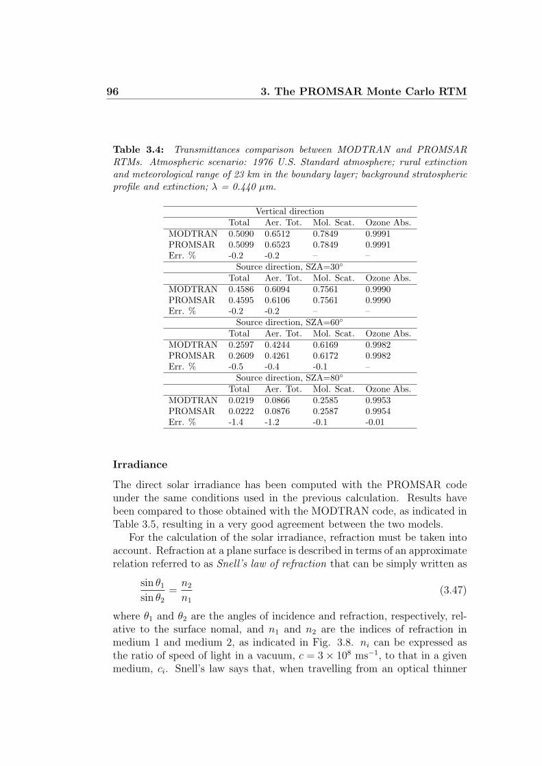
96 3. The PROMSAR Monte Carlo RTM
Table 3.4: Transmittances comparison between MODTRAN and PROMSARRTMs. Atmospheric scenario: 1976 U.S. Standard atmosphere; rural extinctionand meteorological range of 23 km in the boundary layer; background stratosphericprofile and extinction; λ = 0.440 µm.
Vertical directionTotal Aer. Tot. Mol. Scat. Ozone Abs.
MODTRAN 0.5090 0.6512 0.7849 0.9991PROMSAR 0.5099 0.6523 0.7849 0.9991Err. % -0.2 -0.2 – –
Source direction, SZA=30
Total Aer. Tot. Mol. Scat. Ozone Abs.MODTRAN 0.4586 0.6094 0.7561 0.9990PROMSAR 0.4595 0.6106 0.7561 0.9990Err. % -0.2 -0.2 – –
Source direction, SZA=60
Total Aer. Tot. Mol. Scat. Ozone Abs.MODTRAN 0.2597 0.4244 0.6169 0.9982PROMSAR 0.2609 0.4261 0.6172 0.9982Err. % -0.5 -0.4 -0.1 –
Source direction, SZA=80
Total Aer. Tot. Mol. Scat. Ozone Abs.MODTRAN 0.0219 0.0866 0.2585 0.9953PROMSAR 0.0222 0.0876 0.2587 0.9954Err. % -1.4 -1.2 -0.1 -0.01
Irradiance
The direct solar irradiance has been computed with the PROMSAR codeunder the same conditions used in the previous calculation. Results havebeen compared to those obtained with the MODTRAN code, as indicated inTable 3.5, resulting in a very good agreement between the two models.
For the calculation of the solar irradiance, refraction must be taken intoaccount. Refraction at a plane surface is described in terms of an approximaterelation referred to as Snell’s law of refraction that can be simply written as
sin θ1
sin θ2
=n2
n1
(3.47)
where θ1 and θ2 are the angles of incidence and refraction, respectively, rel-ative to the surface nomal, and n1 and n2 are the indices of refraction inmedium 1 and medium 2, as indicated in Fig. 3.8. ni can be expressed asthe ratio of speed of light in a vacuum, c = 3× 10⁸ ms−1, to that in a givenmedium, ci. Snell’s law says that, when travelling from an optical thinner

3.4 Sample applications of the PROMSAR code 97
Table 3.5: Direct irradiance comparison between MODTRAN and PROMSARRTMs. Atmospheric scenario: 1976 U.S. Standard atmosphere; rural extinctionand meteorological range of 23 km in the boundary layer; background stratosphericprofile and extinction; λ = 0.440 µm.
SZA MODTRAN PROMSAR Err. %30 1.52E-06 1.52E-06 –60 8.60E-07 8.63E-07 -0.380 7.26E-08 7.34E-08 -1
Figure 3.8: Examples of reflection and refraction. During refraction, the anglesof incidence and refraction are related by the Snell’s law.
into an optical thicker medium, light is refracted towards the vertical. In theatmosphere, therefore, light is bent towards the normal while travelling fromthe sun to the surface. Atmospheric refraction depends on wavelength (largerfor shorter wavelengths), on density and thus air humidity and temperature,and it is largest in the troposphere.In order to check the correct treatment of the refraction phenomenon whichoccurs in the atmosphere, the main parameters which are used in the MOD-TRAN code to describe the refraction have been computed by the PROM-SAR code. The comparison between the two model outputs is summarisedin Table 3.6. Figure 3.9 moreover shows a graphical representation of suchparameters, allowing to better understand their physical meaning. Considerthe optical path through the atmosphere from point a to b as shown in Fig.3.9. The path is defined by the initial and final altitudes za and zb and by thezenith angle θ at a. The other path quantities are: S, the curved path lengthfrom a (“total range” in Table 3.6); β, the Earth-centered angle (“earth cen-tre angle” in Table 3.6); φ, the zenith angle at b (“entrance angle” in Table
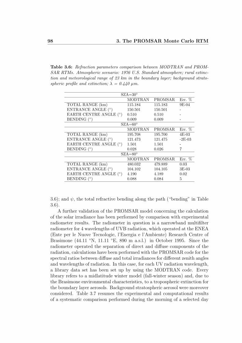
98 3. The PROMSAR Monte Carlo RTM
Table 3.6: Refraction parameters comparison between MODTRAN and PROM-SAR RTMs. Atmospheric scenario: 1976 U.S. Standard atmosphere; rural extinc-tion and meteorological range of 23 km in the boundary layer; background strato-spheric profile and extinction; λ = 0.440 µm.
SZA=30
MODTRAN PROMSAR Err. %TOTAL RANGE (km) 115.184 115.183 9E-04ENTRANCE ANGLE () 150.501 150.501 -EARTH CENTRE ANGLE () 0.510 0.510 -BENDING () 0.009 0.009 -
SZA=60
MODTRAN PROMSAR Err. %TOTAL RANGE (km) 195.708 195.700 4E-03ENTRANCE ANGLE () 121.473 121.475 -2E-03EARTH CENTRE ANGLE () 1.501 1.501 -BENDING () 0.028 0.026 7
SZA=80
MODTRAN PROMSAR Err. %TOTAL RANGE (km) 480.032 479.889 0.03ENTRANCE ANGLE () 104.102 104.105 3E-03EARTH CENTRE ANGLE () 4.190 4.189 0.02BENDING () 0.088 0.084 5
3.6); and ψ, the total refractive bending along the path (“bending” in Table3.6).
A further validation of the PROMSAR model concerning the calculationof the solar irradiance has been performed by comparison with experimentalradiometer results. The radiometer in question is a narrowband multifilterradiometer for 4 wavelengths of UVB radiation, which operated at the ENEA(Ente per le Nuove Tecnologie, l’Energia e l’Ambiente) Research Centre ofBrasimone (44.11 N, 11.11 E, 890 m a.s.l.) in October 1995. Since theradiometer operated the separation of direct and diffuse components of theradiation, calculations have been performed with the PROMSAR code for thespectral ratios between diffuse and total irradiances for different zenith anglesand wavelengths of radiation. In this case, for each UV radiation wavelength,a library data set has been set up by using the MODTRAN code. Everylibrary refers to a midlatitude winter model (fall-winter season) and, due tothe Brasimone environmental characteristics, to a tropospheric extinction forthe boundary layer aerosols. Background stratospheric aerosol were moreoverconsidered. Table 3.7 resumes the experimental and computational resultsof a systematic comparison performed during the morning of a selected day
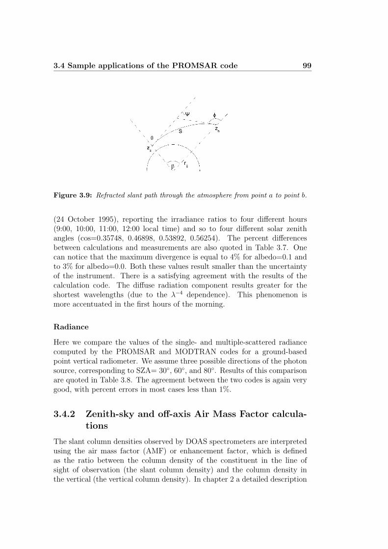
3.4 Sample applications of the PROMSAR code 99
Figure 3.9: Refracted slant path through the atmosphere from point a to point b.
(24 October 1995), reporting the irradiance ratios to four different hours(9:00, 10:00, 11:00, 12:00 local time) and so to four different solar zenithangles (cos=0.35748, 0.46898, 0.53892, 0.56254). The percent differencesbetween calculations and measurements are also quoted in Table 3.7. Onecan notice that the maximum divergence is equal to 4% for albedo=0.1 andto 3% for albedo=0.0. Both these values result smaller than the uncertaintyof the instrument. There is a satisfying agreement with the results of thecalculation code. The diffuse radiation component results greater for theshortest wavelengths (due to the λ−4 dependence). This phenomenon ismore accentuated in the first hours of the morning.
Radiance
Here we compare the values of the single- and multiple-scattered radiancecomputed by the PROMSAR and MODTRAN codes for a ground-basedpoint vertical radiometer. We assume three possible directions of the photonsource, corresponding to SZA= 30, 60, and 80. Results of this comparisonare quoted in Table 3.8. The agreement between the two codes is again verygood, with percent errors in most cases less than 1%.
3.4.2 Zenith-sky and off-axis Air Mass Factor calcula-tions
The slant column densities observed by DOAS spectrometers are interpretedusing the air mass factor (AMF) or enhancement factor, which is definedas the ratio between the column density of the constituent in the line ofsight of observation (the slant column density) and the column density inthe vertical (the vertical column density). In chapter 2 a detailed description

100 3. The PROMSAR Monte Carlo RTM
Table 3.7: Diffuse to global irradiance ratio experiment-PROMSAR comparison(a=albedo). Atmospheric scenario: Midlatitude winter atmosphere; troposphericextinction and meteorological range of 50 km in the boundary layer; backgroundstratospheric profile and extinction; ha=0.9 km.
cos = 0.35748 (9:00 a.m.)λ(nm) Measured a=0.0 Diff. % a=0.1 Diff. %318 0.880 0.875 0.6 0.880 -312 0.899 0.894 0.6 0.898 0.1305 0.918 0.931 -1.4 0.933 -1.6300 0.965 0.978 -1.3 0.978 -1.3
cos = 0.46898 (10:00 a.m.)λ(nm) Measured a=0.0 Diff. % a=0.1 Diff. %318 0.771 0.774 -0.4 0.782 -1.4312 0.801 0.794 0.9 0.802 -0.1305 0.823 0.823 - 0.830 -0.9300 0.877 0.852 2.9 0.857 2.3
cos = 0.53892 (11:00 a.m.)λ(nm) Measured a=0.0 Diff. % a=0.1 Diff. %318 0.701 0.716 -2.1 0.727 -3.6312 0.732 0.734 -0.3 0.744 -1.6305 0.754 0.754 - 0.762 -1.1300 0.777 0.780 -0.4 0.787 -1.3
cos = 0.56254 (12:00 a.m.)λ(nm) Measured a=0.0 Diff. % a=0.1 Diff. %318 0.681 0.698 -2.5 0.709 -4.1312 0.712 0.715 -0.4 0.726 -2.0305 0.737 0.733 0.5 0.742 -0.7300 0.747 0.767 -2.6 0.774 -3.6
of the AMFs useful for the interpretation of MAX-DOAS measurements wasgiven. It has been shown that the MAX-DOAS configuration is particularlysuitable for the derivation of the trace gases abundance in the troposphereand boundary layer.
Zenith-sky AMF
As already explained in chapter 2, before the off-axis and Multiple AXisDOAS spectrometers became attractive for the measurement of troposphericconstituents, ground-based spectrometers pointing the zenith were being usedto investigate the stratospheric trace gases. However, from zenith-sky mea-surements, information about the tropospheric absorbers can be achieved tosome degree. From the zenith-sky slant column’s diurnal cycle, in fact, it can

3.4 Sample applications of the PROMSAR code 101
Table 3.8: Total single- and multiple- scattered radiance comparison betweenMODTRAN and PROMSAR. Atmospheric scenario: 1976 U.S. Standard atmo-sphere; rural extinction and meteorological range of 23 km in the boundary layer;background stratospheric profile and extinction; λ = 0.440 µm.
SZA=30
Single-scattered radiance (single + multiple)-scattered radianceMODTRAN 2.27E-07 3.17E-07PROMSAR 2.28E-07 3.18E-07Err. % -0.4 -0.3
SZA=60
Single-scattered radiance (single + multiple)-scattered radianceMODTRAN 5.64E-08 1.12E-07PROMSAR 5.66E-08 1.19E-07Err. % -0.4 -6
SZA=80
Single-scattered radiance (single + multiple)-scattered radianceMODTRAN 1.65E-08 4.58E-08PROMSAR 1.66E-08 4.68E-08Err. % -0.6 2
be determined if a gas mainly absorbs in the troposphere or in the strato-sphere. In this section we report two examples which illustrate this idea.We have considered the vertical profile of nitrogen dioxide provided withinthe “1976 U.S. Standard” atmosphere. It is shown in Fig. 3.10. We have thenconsidered the same vertical profile of nitrogen dioxide, but only the valuesfrom the ground until 2 km (see Fig. 3.11), so as to treat the case of a tracegas in the boundary layer (we could have used the profile of a gas that wereally know to be only located in the boundary layer/lower troposphere, suchas, for example, the formaldeyde). Two radiative transfer calculations havebeen carried out with the PROMSAR model for the computation of the airmass factor of nitrogen dioxide at 440 nm, for the vertical profiles depicted inFigs. 3.10 and 3.11. For both the cases, we have used this model atmosphere:1976 U.S. Standard atmosphere, rural aerosol extinction and meteorologicalrange=23 km in the boundary layer, background stratospheric profile andextinction. The single and multiple scattering AMFs of the “stratospheric”and “tropospheric” nitrogen dioxide, and their percent differences are shownin Tables 3.9 and 3.10, respectively. It can be noticed that the percent dif-ferences between the single and multiple scattering AMFs shown in Table 3.9are lower than those shown in Table 3.10. This indicates that, even if the airmass factor for the zenith sky configuration increases with multiple scatter-

102 3. The PROMSAR Monte Carlo RTM
Figure 3.10: NO2 vertical profile provided by the 1976 U.S. Standard atmosphericmodel.
Figure 3.11: NO2 vertical profile between 0 and 2 km provided by the 1976 U.S.Standard atmospheric model.
ing, the single scattering model can be considered a good approximation forstratospheric absorbers. However, when considering an absorber in the lowertroposphere, multiple scattering has a consequence on the radiation transferand, therefore, must be taken into account. The air mass factors listed inTables 3.9 and 3.10 are shown in Fig. 3.12. As already pointed out (also insection 2.4), the dependence of the zenith-sky AMF on the solar zenith angleallows to identify either a trace gas is mainly located in the stratosphere orin the troposphere. For a stratospheric absorber like that shown in Fig. 3.10,the slant column and, hence, the air mass factor, increases with increasingSZA (see Fig. 3.12, blue lines) as long as the scattering height lies initiallybelow and then within the absorbing layer. If at very low sun the most likelyscattering height is situated above the absorbing layer the slant column de-

3.4 Sample applications of the PROMSAR code 103
Table 3.9: NO2 AMF for single scattering approximation and multiple scatter-ing at 440 nm. Atmospheric scenario: 1976 U.S. Standard atmosphere; ruralextinction and meteorological range of 23 km in the boundary layer; backgroundstratospheric profile and extinction.
SZA() NO2 AMF NO2 AMF Diff. %single scattering multiple scattering
5 1.004 1.015 110 1.015 1.031 215 1.034 1.054 220 1.062 1.087 225 1.099 1.130 330 1.148 1.186 335 1.211 1.257 440 1.291 1.347 445 1.393 1.459 550 1.524 1.606 555 1.697 1.793 560 1.929 2.044 665 2.255 2.388 670 2.734 2.894 675 3.501 3.695 580 4.883 5.134 585 7.935 8.290 590 16.87 17.35 391 20.10 20.56 292 23.64 23.87 193 27.07 27.13 0.294 28.62 29.02 195 26.07 28.98 10
creases in turn.Instead, a trace gas in the lower troposphere (Fig. 3.11) absorbs below themost likely scattering height along a relatively short light path which changesonly slightly with the solar zenith angle. By consequence, its slant columnand, hence, air mass factor varies only slightly with the solar zenith angle(see Fig. 3.12, green lines).
Off-axis AMF
With regard to the AMF calculation in the off-axis/multiple axis geometry,several examples have been already shown in chapter 2, section 2.4.1. Inthis section, we just restrict ourselves to show two further examples of AMF
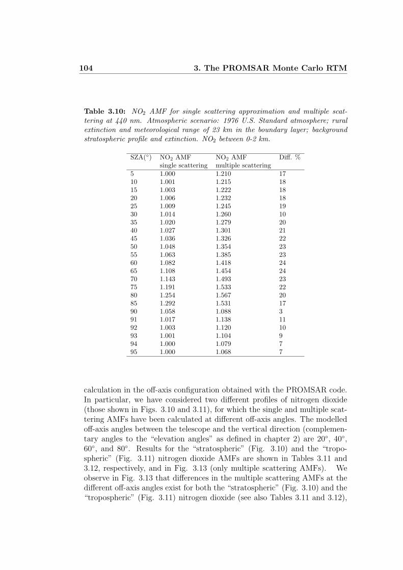
104 3. The PROMSAR Monte Carlo RTM
Table 3.10: NO2 AMF for single scattering approximation and multiple scat-tering at 440 nm. Atmospheric scenario: 1976 U.S. Standard atmosphere; ruralextinction and meteorological range of 23 km in the boundary layer; backgroundstratospheric profile and extinction. NO2 between 0-2 km.
SZA() NO2 AMF NO2 AMF Diff. %single scattering multiple scattering
5 1.000 1.210 1710 1.001 1.215 1815 1.003 1.222 1820 1.006 1.232 1825 1.009 1.245 1930 1.014 1.260 1035 1.020 1.279 2040 1.027 1.301 2145 1.036 1.326 2250 1.048 1.354 2355 1.063 1.385 2360 1.082 1.418 2465 1.108 1.454 2470 1.143 1.493 2375 1.191 1.533 2280 1.254 1.567 2085 1.292 1.531 1790 1.058 1.088 391 1.017 1.138 1192 1.003 1.120 1093 1.001 1.104 994 1.000 1.079 795 1.000 1.068 7
calculation in the off-axis configuration obtained with the PROMSAR code.In particular, we have considered two different profiles of nitrogen dioxide(those shown in Figs. 3.10 and 3.11), for which the single and multiple scat-tering AMFs have been calculated at different off-axis angles. The modelledoff-axis angles between the telescope and the vertical direction (complemen-tary angles to the “elevation angles” as defined in chapter 2) are 20, 40,60, and 80. Results for the “stratospheric” (Fig. 3.10) and the “tropo-spheric” (Fig. 3.11) nitrogen dioxide AMFs are shown in Tables 3.11 and3.12, respectively, and in Fig. 3.13 (only multiple scattering AMFs). Weobserve in Fig. 3.13 that differences in the multiple scattering AMFs at thedifferent off-axis angles exist for both the “stratospheric” (Fig. 3.10) and the“tropospheric” (Fig. 3.11) nitrogen dioxide (see also Tables 3.11 and 3.12),

3.4 Sample applications of the PROMSAR code 105
Figure 3.12: Nitrogen dioxide air mass factors at 440 nm computed with thePROMSAR model for a stratospheric (Fig. 3.10) and a tropospheric/boundarylayer (Fig. 3.11) vertical profile of the absorber. Dashed and solid lines indicate,respectively, single and multiple scattering AMFs.
but they are especially evident in the case of the absorber located in thelower troposphere, as expected. On the other hand, the air mass factors forthe horizon viewing mode are slightly increased by multilpe scattering forhigh sun, but clearly decreased at low sun.

106 3. The PROMSAR Monte Carlo RTM
Table 3.11: NO2 AMF for single/multiple scattering at 440 nm and for fouroff-axis angles (20, 40, 60, 80). Atmospheric scenario: 1976 U.S. Standardatmosphere; rural extinction and meteorological range of 23 km in the boundarylayer; background stratospheric profile and extinction.
OA=20 OA=40 OA=60 OA=80
SZA() s.s m.s. % s.s m.s % s.s m.s % s.s m.s %5 1.008 1.035 2.6 1.021 1.082 5.6 1.052 1.161 9.4 1.08 1.21 10.710 1.019 1.041 2.1 1.032 1.085 4.9 1.062 1.163 8.7 1.096 1.214 9.715 1.037 1.053 1.5 1.051 1.096 4.1 1.081 1.171 7.7 1.114 1.224 9.020 1.064 1.066 0.2 1.078 1.117 3.5 1.108 1.191 7.0 1.142 1.246 8.325 1.1 1.118 1.6 1.115 1.148 2.9 1.146 1.22 6.1 1.179 1.276 7.630 1.147 1.173 2.2 1.163 1.193 2.5 1.195 1.261 5.2 1.229 1.321 7.035 1.208 1.242 2.7 1.224 1.246 1.8 1.258 1.318 4.6 1.293 1.378 6.240 1.285 1.33 3.4 1.302 1.305 0.2 1.339 1.392 3.8 1.375 1.456 5.645 1.385 1.441 3.9 1.402 1.427 1.8 1.442 1.489 3.2 1.482 1.557 4.850 1.513 1.585 4.5 1.529 1.568 2.5 1.574 1.617 2.7 1.62 1.689 4.155 1.682 1.773 5.1 1.698 1.75 3.0 1.745 1.78 2.0 1.802 1.866 3.460 1.908 2.024 5.7 1.926 1.995 3.5 1.977 1.984 0.4 2.05 2.108 2.865 2.224 2.367 6.0 2.244 2.334 3.9 2.302 2.347 1.9 2.398 2.449 2.170 2.688 2.87 6.3 2.71 2.829 4.2 2.772 2.843 2.5 2.912 2.956 1.575 3.421 3.652 6.3 3.446 3.606 4.4 3.518 3.621 2.8 3.725 3.756 0.880 4.727 5.037 6.2 4.755 4.98 4.5 4.837 4.994 3.1 5.169 5.173 0.185 7.593 8.063 5.8 7.676 8.001 4.1 7.773 8.008 2.9 8.068 8.138 0.990 15.82 17.17 7.9 16.75 17.43 3.9 17.56 17.67 0.6 17.2 17.23 0.291 18.12 19.81 8.5 19.21 20.22 5.0 20.7 20.76 0.3 20.75 20.39 -1.892 20.7 22.12 6.4 21.35 22.38 4.6 22.89 23.08 0.8 24.29 23.27 -4.493 22.02 23.38 5.8 22.22 23.32 4.7 24.1 24.41 1.3 27.21 25.15 -8.294 21.88 22.76 3.9 21.8 22.66 3.8 22.35 23.63 5.4 25.96 23.43 -10.895 19.5 19.32 -0.9 20.12 20.32 1.0 21.91 21.76 -0.7 26.78 23.82 -12.4

3.4 Sample applications of the PROMSAR code 107
Table 3.12: NO2 AMF for single/multiple scattering at 440 nm and for fouroff-axis angles (20, 40, 60, 80). Atmospheric scenario: 1976 U.S. Standardatmosphere; rural extinction and meteorological range of 23 km in the boundarylayer; background stratospheric profile and extinction. NO2 between 0-2 km.
OA=20 OA=40 OA=60 OA=80
SZA() s.s m.s. % s.s m.s % s.s m.s % s.s m.s %5 1.047 1.13 7.3 1.226 1.429 14.2 1.729 2.161 20.0 3.593 4.502 20.210 1.05 1.119 6.2 1.227 1.404 12.6 1.727 2.129 18.9 3.578 4.455 19.715 1.055 1.104 4.4 1.231 1.384 11.1 1.724 2.086 17.4 3.559 4.398 19.120 1.064 1.07 0.6 1.238 1.372 9.8 1.729 2.065 16.3 3.558 4.363 18.525 1.076 1.129 4.7 1.248 1.363 8.4 1.736 2.04 14.9 3.555 4.315 17.630 1.089 1.167 6.7 1.262 1.361 7.3 1.748 2.023 13.6 3.573 4.297 16.835 1.105 1.204 8.2 1.278 1.352 5.5 1.765 2.014 12.4 3.591 4.27 15.940 1.125 1.25 10.0 1.305 1.314 0.7 1.79 2.015 11.2 3.634 4.283 15.245 1.149 1.304 11.9 1.339 1.421 5.8 1.822 2.023 9.9 3.689 4.295 14.150 1.177 1.367 13.9 1.372 1.495 8.2 1.864 2.042 8.7 3.767 4.321 12.855 1.209 1.439 16.0 1.415 1.571 9.9 1.914 2.05 6.6 3.876 4.85 20.160 1.245 1.519 18.0 1.465 1.66 11.7 1.999 2.016 0.8 4.028 4.484 10.265 1.287 1.599 19.5 1.526 1.795 15.0 2.109 2.253 6.4 4.238 4.634 8.570 1.323 1.679 21.2 1.591 1.861 14.5 2.217 2.416 8.2 4.54 4.859 6.675 1.348 1.715 21.4 1.645 1.943 15.3 2.342 2.569 8.8 4.965 5.163 3.880 1.301 1.668 22.0 1.625 1.929 15.8 2.41 2.647 9.0 5.735 5.74 0.185 1.132 1.45 21.9 1.41 1.706 17.4 2.173 2.432 10.6 6.306 5.942 -6.190 1.064 1.325 19.7 1.305 1.568 16.8 1.999 2.269 11.9 5.736 5.388 -6.591 1.064 1.328 19.9 1.305 1.569 16.8 1.999 2.271 12.0 5.736 5.392 -6.492 1.064 1.338 20.5 1.305 1.574 17.1 1.999 2.283 12.4 5.736 5.402 -6.293 1.064 1.357 21.6 1.305 1.582 17.5 1.999 2.31 13.5 5.736 5.404 -6.194 1.064 1.387 23.3 1.305 1.605 18.7 1.999 2.355 15.1 5.736 5.379 -6.695 1.064 1.399 23.9 1.305 1.644 20.6 1.999 2.372 15.7 5.736 5.318 -7.9

108 3. The PROMSAR Monte Carlo RTM
Figure 3.13: Nitrogen dioxide air mass factors at 440 nm computed with thePROMSAR model for the stratospheric NO2 vertical profile shown in Fig. 3.10(top) and the tropospheric NO2 vertical profile shown in Fig. 3.11 (bottom), andfor four off-axis angles (20, 40, 60, 80).

Chapter 4
Remote sensing and theretrieval problem
Remote Sensing is the science and art of obtaining informationabout an object, area, or phenomenon through the analysis ofdata acquired by a device that is not in contact with the object,area, or phenomenon under investigation.T. M. Lillesand and M. W. Kiefer, Remote Sensing andImage Interpretation
Remote Sensing is defined as the acquisition of informationabout an object without being in physical contact with it.C. Elachi, Introduction To The Physics and Techniquesof Remote Sensing
Remote Sensing is the science of acquiring, processing andinterpreting images that record the interaction betweenelectromagnetic energy and matter.F. F. Sabins, Remote sensing: principles andinterpretation
Broadly speaking, remote sensing is a way of obtaining information aboutproperties of an object or volume without coming into physical contact withthat object. We may so consider remote sensing to be an indirect measure-ment method, i.e. we do not measure directly but by means of, for instance,electromagnetic radiation as an information carrier.
Problems of remote sensing fall into a category referred to as inverseproblems. The nature of these inverse problems is portrayed in Fig. 4.1 inthe form of an analogy, and can be posed in the following way. How wellcan we infer the animal from observations of its tracks? Clearly this line of

110 4. Remote sensing and the retrieval problem
inquiry is fruitless without a priori knowledge of animals and the types oftracks they leave.
Figure 4.1: The nature of inverse problems, from Stephens [54].
The atmosphere is a typical subject for which remote sensing measure-ments are effective, and for which inverse methods are required. Thereforea central theme in remote sensing of the atmosphere is the understandingof how electromagnetic radiation interacts with matter since these are thetracks we exploit to infer information about the atmosphere.The example dealt with in this thesis is one in which electromagnetic ra-diation emerging from the atmosphere is measured by a spectrometer andprocessed by the DOAS algorithm to obtain the slant column density of atrace gas (i.e. the integrated concentration along the light path), when thequantity required is the vertical profile of the trace gas in question. Of course,the slant column density is a function of the trace gas vertical profile we wantto obtain. So, we have to retrieve the unknown quantity we are interested infrom the measurements made. This reconstruction is called “retrieval”.
The usual approach to solving a retrieval problem in the frame of theatmospheric sciences consists of several stages: design a forward model todescribe the physics of the measurement and the instrument; determine thecriterion by which a solution is acceptable as valid; construct a numericalmethod to find a solution which satisfies the criterion; carry out an erroranalysis, validate the process by reference to internal diagnostics and inde-pendent measurements, and finally attempt to understand how the resultobtained is related to reality and examine how much information has been

4.1 Atmospheric remote sensing 111
obtained and with which reliability.
4.1 Atmospheric remote sensing
How well can we infer the animal from observations of itstracks?
4.1.1 The beginnings
Atmospheric inverse problems began in 1920’s when Dobson started to makemeasurements of ozone in the stratosphere using an ultraviolet spectrometeron the ground. The initial measurements were of total ozone, based onabsorption of solar ultraviolet light, but it was realized by Gotz in 1930 thatby measuring the Rayleigh scattered sunlight from the zenith sky as thesun sets it is possible to obtain information about the vertical distributionof ozone [55]. This is the so-called Umkehr method. The word umkehrmeans “reversal” and refers to the time variation of the ratio of the scatteredintensity at two different wavelengths. Methods for deriving the verticaldistribution from the umkehr curve were developed by Gotz, Dobson andMeetham [15]. It was not until Mateer [56] carried out its seminal work onthe information content of umkehr observations that the subject was put ona firm footing.
With the advent of meteorological satellites, it became clear that remotemeasurements from space would be very important in determining the stateof the atmosphere globally. Kaplan [57] proposed that the vertical distri-bution of temperature in the atmosphere could be determined globally bymeasuring from satellites, as a function of wavelength, the thermal emissionfrom the 15 µm band of carbon dioxide, and also pointed out that ozoneand water vapour should also be amenable to remote measurement. Kaplanonly gave a qualitative suggestion about how the profiles might be retrieved;detailed methods were developed by Wark [58] and Yamamoto [59] in two ofthe earliest papers on the subject of inverse theory for atmospheric remotesounding from satellites.
4.1.2 Atmospheric remote sensing methods
Remote sensing of the atmosphere has been carried out by a wide variety ofinstruments, using many different principles of measurement and platforms.Almost all techniques involve the measurement of electromagnetic radiation.The physical effects exploited may involve extinction, scattering, absorption,
112 4. Remote sensing and the retrieval problem
emission at all wavelengths from radio to the ultraviolet. The measurementtechniques and instruments include spectrometers, interferometers, radiome-ters, gas correlation methods, microwave and radio receivers. Most methodsare passive, measuring naturally generated radiation, but some (e.g. lidar)are active in that they use man-made sources.
As already pointed out, the first remote measurements of the atmosphericcomposition was of total ozone using absorption of solar radiation. Thesame principle can be used for the measurement of a wide variety of gases,particularly in the infrared and microwave, where many constituents haveabsorption lines and bands, but also in the ultraviolet and visible, as in thecase of Differential Optical Absorption Spectroscopy.
In the following sections, we will briefly discuss the theoretical basis ofretrieval problems, especially following the work of Rodgers. A special inver-sion method, the Chahine relaxation method, will be in particular described.In chapter 5, the application of the Chahine relaxation method to a set ofslant column densities measured by a MAX-DOAS instrument will be dis-cussed, and the retrieved NO2 and ozone vertical profiles will be presentedin detail.
4.2 Information aspects in retrieval methods
Different remote sensing problems and related retrieval methods reduce tofind the solution of equations like or similar to
g(y) =
∫ b
a
K(y, x)f(x)dx a ≤ y ≤ b, (4.1)
where the limits of the integral depend on the details of the problem athand. This equation is known as the Fredholm integral equation of the firstkind because the limits of the integral are fixed and because the unknown,f(x), appears only in the integrand. The function K(y, x) is known as thekernel or kernel function. f(x) can be obtained by solving Eq. 4.1 when g(y)is the observation at various y values and the kernel is known. Solution to Eq.4.1 requires inversion to obtain the distribution f(x). This is an unfotunatecircumstance since the solutions to Eq. 4.1 suffer a number of difficulties,including non-existence, non-uniqueness, and instability. Non-existence isusually not an issue for most practical problems since we measure g(y) andf(x) exists through physical considerations. Non-uniqueness is related to ablurring effect or a departure from one-to-one correspondence between f(x)and g(y): there exist several functions f(x) which produce the same functiong(y). This problem tends to be overcome to a certain extent by restricting the

4.2 Information aspects in retrieval methods 113
class of admissible solutions to physically realizable ones. In this way, a prioriinformation is introduced into the retrieval scheme. The major difficulty insolving Eq. 4.1, at least for most practical problems, concerns the problemof instability which arises, for example, from errors in the observations g(y).With a small error ε(y) in g(y), Eq. 4.1 becomes
g(y) + ε(y) =
∫ b
a
K(y, x)f(x)dx, (4.2)
where ε(y) produces an arbitrary large change in f(x) and the ultimate suc-cess of any retrieval largely depends on the accuracy of the measurement g(y)and on the shape of K(y, x).
In most practical situations, numerical methods are used for inversion ofEq. 4.1. A full overview of these methods and their applications can befound in [60]. An important contribution to these issues came from Rodgers,who worked to the formal statement of the problem, which also includes atreatment of errors (see e.g. [61] and [62]).
4.2.1 Formal statement of the problem
The general inverse problem can be regaded as a question of setting up andsolving a set of simultaneous linear or non-linear equations, in the presenceof experimental error in some of the parameters (the “measurements”), andquite possibly in the presence of approximations in the formulation of theequations. To examine the information content of the indirect measurement,we will cosider the measurements assembled into a vector ~y, the measure-ment vector, and the unknowns into a state vector ~x, describing the state ofthe atmosphere. Some aspects of the state of the atmosphere, for examplethe trace gases distribution, are properly described by continuous functionsrather than discrete values, but ways can always be found of approximatingcontinuous functions by discrete values to any desired accuracy. The processof measurement will be described by a forward model, which describes thephysics of the measurement process.
State and measurement vectors
The quantities to be retrieved can be represented by a state vector, ~x, withn elements, x1, x2, · · · , xn. Often it will represent a profile of some quantitygiven at a finite number of levels, enough to adequately represent the possibleatmospheric variations.
The quantity actually measured in order to retrieve ~x can be representedby the measurement vector ~y, with m elements, y1, y2, · · · , ym. This vector

114 4. Remote sensing and the retrieval problem
should include all the quantities measured that are functions of the statevector. Measurements are made to a finite accuracy; random error or mea-surement noise will be denoted by the vector ε.
The forward model
For each state vector there is a corresponding ideal measurement ~yI , de-termined by the physics of the measurement. We can describe the physicsformally as the forward function f(~x), so that
~yI = f(~x). (4.3)
However, in practice not only is there always experimental error, but it isoften necessary to approximate the detailed physics by some forward modelF (~x). Therefore we will write the relationship between the measurementvector and the state vector as
~y = F (~x) + ε, (4.4)
where the vector ~y is the measurement with error ε, and F (~x) is a vectorvalued function of the state, which encapsulates our understanding of thephysics of the measurement. To construct a forward model we must of courseknow how the device works, and understand how the quantity measured isrelated to the quantity that is really wanted. F is described as a modelbecause there may be underlying physics which is not fully understood, orthe real physics may be so complicated that approximations are necessary.
The quantities to be retrieved in most inverse problems are continuousfunctions, while the measurements are always of discrete quantities. Thusmost inverse problems are formally ill-posed or underconstrained in this triv-ial sense. This is simply dealt with by replacing the truly continuous statefunction, corresponding to a finite number of variables, with a representa-tion in terms of a finite number of parameters. This can be done to whateverspatial resolution or degree of accuracy is required for scientific use of theretrieval, e.g., the profile of a trace gas could be represented on a finite gridof points with a spacing appropriate to the application. After discretisationthe problem may or may not be underconstrained, depending on the gridspacing required and the information content of the measurement.
Weighting function matrix
For the purpose of examining the information content of a measurement itis most convenient to consider a linear problem. A linearisation of the for-ward model about some reference state ~x0 will be adequate for this purpose,
4.2 Information aspects in retrieval methods 115
provided that F (~x) is linear within the error bounds of the retrieval. Write
~y = F (~x0) +∂F (~x)
∂~x(~x− ~x0) + ε (4.5)
~y − F (~x0) =∂F (~x)
∂~x(~x− ~x0) + ε (4.6)
~y − F (~x0) = K(~x− ~x0) + ε, (4.7)
which defines the m×n weighting function matrix K, not necessarily square,in which each element is the partial derivative of a forward model elementwith respect to a state vector element, i.e., Kij = ∂Fi(~x)/∂~xj. Derivativeof this type are known as Frechet derivatives. If m < n the equations aredescribed as underconstrained because there are fewer measurements thanunknowns. Similarly, if m > n the equations are often described as overcon-strained.
Vector spaces
The concept of a linear vector space is very useful in considering linear equa-tions. We will give two such spaces special names: the state space is a vectorspace of dimension n within which each conceivable state is represented by apoint, or equivalently by a vector from the origin (x0) to the point. The mea-surement space is a vector space of dimension m, in which each conceivablemeasurement is likewise represented by a point or a vector (with the originat F (x0)). The act of measurement is then equivalent to a mapping fromthe state space into the measurement space, and the inverse problem is thatof finding an appropriate inverse mapping from the measurement space backinto the state space. The weighting function matrix K represents the forwardmapping, equivalent to the measurement apart from the measurement errorε. Each row of K, of dimension n, can be thought of as a vector ki in statespace. It corresponds to the ith measurement yi in the sense that the valueof the ith coordinate of measurement space for a given state vector ~x is thevector product of ~x and ki, plus measurement error. Thus each of the mrows of K corresponds to a coordinate in measurement space, providing themapping from state space to measurement space.
4.2.2 Linear problems without measurement error
Consider first a linear problem with arbitary numbers of dimensions in theabsence of measurement error. In this case the problem reduces to the exactsolution of linear simulatneous equations,
~y = K~x, (4.8)

116 4. Remote sensing and the retrieval problem
and involves determining how many solutions exist, if they exist. More gen-erally, it is a matter of investigating what information can be extracted fromthe measurements ~y about the space ~x particularly when there is no solutionor no unique solution.
The m weighting function vectors kj will span some subspace of statespace which will be of dimension not greater then m, and may be less thanm if the vectors are not linearly independent. The dimension of this sub-space is known as the rank of the matrix K, denoted by p, and is equal to thenumber of linearly independent rows. If m > n, more measurements thanunknowns, then the rank cannot be greater than n. The subspace spannedby the vectors forming the rows of K is called the row space of K. K also hasa column space of dimension p which is a subspace of measurement space.We can imagine an orthogonal coordinate system or base for the state spacewhich has p orthogonal base vectors in row space, and n−p base vectors out-side which are orthogonal to row space and, therefore, to all of the weightingfunction vectors. The components of the state vector orthogonal to row spacewill give a zero contribution to the measurement, i.e. are unmeasurable. Thispart of the state space is called null space of K.If p < n the null space exists: in this case the solution is non-unique becausethere are components of the state space which are not determined by themeasurements, and which could therefore take any value.
4.2.3 Linear problems with measurement error
All real measurements are subject to experimental errors. The proper treat-ment of such errors is fundamental in designing retrieval methods.A description of experimental error in term of probability density functions(pdf ′s) gives useful insight. The statement that a scalar measurement has avalue y and an error σ is a shorthand way of saying that our knowledge ofthe true value of the measured parameter is described by a pdf P (y) with amean y and a variance σ2:
y =
∫y · P (y)dy (4.9)
σ2 =
∫(y − y)2 · P (y)dy (4.10)
and that the probability that y lies in (y, y+dy) is P (y)dy. The form of P (y)is almost always taken to be Gaussian: this is usually a good approximationfo experimental error, and is very convenient for algebraic manipulations.When the measured quantity is a vector, a probability density can still be

4.3 Error analysis in retrieval methods 117
defined over measurement space, P (~y), with the interpretation that P (~y)d~yis the probability that the true value of the measurement lies in a multidi-mensional interval (~y, ~y + d~y) in measurement space. Different elements of avector may be correlated, in the sense that
Sij = E(yi − yi)(yj − yj) 6= 0, (4.11)
where Sij is called the covariance of yi and yj and E is the expected valueoperator. These covariances can be assembled into a matrix, which we willdenote by Sy for the covariance matrix of ~y. Its diagonal elements are clearlythe variances of the individual elements of ~y. A covariance matrix is sym-metric and non-negative definite, and is almost always positive definite.
4.3 Error analysis in retrieval methods
In this section we will carry out a general characterisation and error analysis,following the methods developed by Eyre [63] and Rodgers [61], that can beapplied to any inverse method and which will show how a retrieval is relatedto the true state of e.g. the atmosphere, and how various sources of errorspropagate into the final product.
4.3.1 Characterisation
The forward model
For any remote measurement, the quantity measured, ~y, is some vector val-ued function f of the unknown state vector, ~x, and of some other set ofparameters, ~b, that we have decided not to include in the state vector. Thereis also an experimental error term, ε. Therefore we write, more generallythan Eq. 4.4:
~y = f(~x,~b) + ε, (4.12)
where the Forward Function f describes the complete physics of the mea-surement, including for example the radiative transfer theory required torelate the state to the measured signal, as well as a full description of themeasuring instrument. The vector of parameters ~b comprises those quanti-ties which influence the measurement, are known to some accuracy, but arenot intended as quantities to be retrieved. They will be termed the forwardfunction parameters and will contribute to the total measurement accuracy.The error term ε includes errors from sources which are not related to theforward function parameters.

118 4. Remote sensing and the retrieval problem
The retrieval method
The retrieval x is the result of operating on the measurement with someRetrieval Method R,
x = R(~y, b, ~xa,~c), (4.13)
where the circumflex does not indicate a true state but an estimated quantity.b is the best estimate of the forward function parameters, the vectors ~xa
and ~c together comprise the parameters that do not appears in the forwardfunction, but do affect the retrieval. ~xa is any a priori estimate of ~x that maybe used and ~c contains any other parameters of this nature. Some inversemethods use an explicit a priori, some do not. The a priori estimate can bethought of as any kind of estimate of the state used in the inverse method andwhich is unrelated to the actual measurement. The parameters comprising ~cwill be called retrieval method parameters.
The transfer function
By substituting Eq. 4.4 into Eq. 4.13, we can relate the retrieval to the truestate:
x = R(f(~x,~b) + ε, b, ~xa,~c). (4.14)
Eq. 4.14 can be regarded as a Transfer Function which describes the way inwhich the whole system can operate, including both the measuring instru-ment and the retrieval method. Understanding the properties of the transferfunction is fundamental to both characterization of the observing system(i.e., the sensitivity of the retrieved to the true state, expressed as ∂x/∂~x)and the error analysis (i.e., the sensitivity of the retrieval to all of the sourcesof error in the transfer function, including noise in the measurement, errorin the non-retrieved parameters and in the retrieval method parameters, andthe effect of modelling the true physics of the measurement by means of aforward model).
Linearisation of the transfer function
The forward function is often a source of difficulty, due to the fact that thereal physics is far too complex (or uncertain) to deal with explicitly. For thatreason, a Forward Model, F , with associated errors, may be used:
F (~x,~b) ∼= f(~x,~b, ~b′) (4.15)

4.3 Error analysis in retrieval methods 119
where ~b has been separated into ~b and ~b′, where ~b′ represents those forwardfunction parameters which are ignored in the construction of the forwardmodel. Replacing the forward function by the forward model, and includingan error term to allow for this, Eq. 4.14 becomes:
x = R[F (~x,~b) + ∆f(~x,~b, ~b′) + ε, b, ~xa,~c], (4.16)
where ∆f is the error in the forward model relative to the real physics:
∆f = f(~x,~b, ~b′)− F (~x,~b). (4.17)
The forward model can be then linearised about ~x = ~xa and ~b = b:
x = R[F (~xa, b)+Kx(~x−~xa)+Kb(~b− b)+∆f(~x,~b, ~b′)+ ε, b, ~xa,~c], (4.18)
where the matrix Kx = ∂F/∂~x is the sensitivity of the forward model to the
state, the weighting function or Jacobian matrix, and Kb = ∂F/∂~b is thesensitivity of the forward model to the forward model parameters. Next, theinverse method can be linearised with respect to its first argument, ~y,
x = R[F (~xa, b), b, ~xa,~c]+Gy[Kx(~x−~xa)+Kb(~b− b)+∆f(~x,~b, ~b′)+ε], (4.19)
where Gy = ∂R/∂~y is the sensitivity of the retrieval to the measurement,which is the same as its sensitivity to measurement error. Rearranging Eq.4.19 we obtain
x− ~xa = R[F (~xa, b), b, ~xa,~c]− ~xa +
+ A(~x− ~xa) +
+Gyεy, (4.20)
where
A = GyKx =∂x
∂~x(4.21)
is the sensitivity of the retrieval to the true state and
εy = Kb(~b− b) + ∆f(~x,~b, ~b′) + ε (4.22)
is the total measurement error in the relative to the forward model.The first term on the right hand side of Eq. 4.20, the bias, is the error
that would result from a simulated retrieval using a simulated error-freemeasurement of the a priori state computed with the forward model. Thea priori represents knowledge of the state before the measurement is made.

120 4. Remote sensing and the retrieval problem
If the measurement were not made, a priori would be our only knowledge.Thus if the measurements are consistent with the state being equal to thea priori, then any “correct” inverse method should return the a priori, i.e.the first term of Eq. 4.20 should be zero. The linearization has been carriedout about the a priori state mainly so that the bias term can be eliminated.Consequently, the above argument can only be applicable to methods usingan explicit a priori.The second term on the right hand side of Eq. 4.20, the smoothing, representsthe way in which the observing system smooths the profile. The differencebetween the retrieval and the linearization point is obtained by operatingon the difference between the true state and the linearization point with thematrix A:
x = ~xa + A(~x− ~xa) +Gyεy = (In − A)~xa + A~x+Gyεy. (4.23)
In the case where the state vector represents a profile, then rows aTi of A
can be regarded as smoothing functions or averaging kernels. In the idealinverse method, A would be a unit matrix. In reality, rows of A are generallypeaked functions, peaking at the appropriate level, and with a half-widthwhich is a measure of the spatial resolution of the observing system, thusproviding a simple characterization of the relationship between the retrievaland the true state. The averaging kernel also has an area, which is foundto be approximately unity at level where the retrieval is accurate, and ingeneral can be thought of as a rough measure of the fraction of the retrievalthat comes from the data, rather than from the a priori.The third term on the right hand side of Eq. 4.20, the retrieval error, isthe error in the retrieval due to the total measurement (εy) which does notinclude the error of the retrieval process.
4.3.2 Error analysis
An expression for the error in x can be obtained by some further rearrange-ments of Eqs. 4.20 and 4.22:
x− ~x = (A− In)(~x− ~xa) +
+GyKb(~b− b) +
+Gy∆f(~x,~b, ~b′) +
+Gyε. (4.24)
The four contributions are, respectively from top to bottom, the smoothingerror, the model parameter error, the forward model error and the retrievalnoise. For a full explanation of such error contributions and related topics,see [62].

4.4 The Chahine inversion method 121
4.4 The Chahine inversion method
In most circumstances the maximum amount of information will be extractedfrom a set of measurements when we use a full non-linear retrieval which min-imises a cost function based on all the data and appropriate a priori. Sincethese methods can be time consuming, approximate and numerically fastmethods can be useful. One possibility is given by the non-linear relaxationmethod whose simplest form was popularised by Chahine [64].A non-linear relaxation method follows the same general idea as the linearrelaxation (see, e.g. [62]), except that the iteration equation is non-linear.At iteration i the value at each level j, xi
j, is modified by multiplying by theratio of the corresponding measured to computed signal, yj/Fj(x
i):
xi+1j = xi
j ·yj
Fj(xi). (4.25)
For well peaked weighting functions, one would expect this to converge to aprofile which produces the right computed signal.Convergence can be analysed by taking logarithms:
lnxi+1j = ln xi
j + [ln yj − lnFj(xi)]. (4.26)
4.4.1 Application of the Chahine inversion method
We have seen in chapter 2 (Eq. 2.2) that the relationship between the zenith-sky slant column density of a given trace gas at a given wavelength λ andsolar zenith angle SZA, yλ(SZA), and its concentration at a given altitudez, cg(z), can be expressed by the following equation
yλ(SZA) =− ln I(SZA,λ)
I0(λ)
σg
=
∫ Z
0
cg(z) · AMFλ(z, SZA) · dz. (4.27)
Assuming that the absorber concentrations remain constant during the mea-surement (e.g. during twilight), the variation in observed zenith-sky slantcolumn with increasing solar zenith angle contains information regarding thevertical profile of the absorber: inversion techniques provide a means of de-termining the profile from such measurements.The evident analogy between Eqs. 4.27 and 4.1 highlights that the air massfactor, AMFλ(z,SZA), is the kernel of Eq. 4.27. Therefore, the retrieval oftrace gases vertical profile relies on forward model calculations of the changesin air mass factor (and hence, slant column density) as a function of SZA.

122 4. Remote sensing and the retrieval problem
In other words, fundamental in the inversion process is modelling the mea-surements through a radiative transfer model, which allows to construct thefollowing linear matrix model
ymi = AMFij · cj (4.28)
where ymi is the modelled (superscript m) slant column at solar zenith angle
i, AMFij is the air mass factor for the trace gas added to layer j, and cj isthe amount of the trace gas in layer j.In principle one can solve Eq. 4.28 for the concentrations in each modelledlayer, in the form
cj = Ajiyoi (4.29)
where Aji is the inverse of AMFij (if it is a square matrix and nonsingu-lar) or some other estimator such as a least squares formulation, and yo
i isthe column amount observed (superscript o) at solar zenith angle i. Un-fortunately, seeking a solution using an unconstrained linear method in thepresence of measurement noise can lead to physically unrasonable solutionssuch as negative amounts in particular atmospheric layers.
The inverse problem may be approached in these cases using the Chahinesolution method, which has been introduced in section 4.4.The solution process is started by assuming a profile, cn=1
j , of the trace gasunder study for the first iteration, a first guess profile. The (nth) iterationsolution profile, cnj , together with the model are used to determine the (n+1)st
estimate of the concentration profile by the equation:
cn+1j = cnj ·
NL∑l=1
[Wjl ·yo
k(j)
ymk(j)
] (4.30)
where k(j) represents the solar zenith angle at which layer j has the largestAMF, NL is the number of layers in the model atmosphere and Wjl are aset of weighting factors that are introduced to stabilize the convergence ofthe solution in the presence of significant correlations between the rows ofthe matrix AMFij. The weighting factors are computed using the followingrelation:
Wjl =AMFk(l)j
AMFk(l)l
(4.31)
for each layer l, and then Wjl are normalized using
Wjl =Wjl∑NLj=1Wjl
. (4.32)

4.4 The Chahine inversion method 123
The iterations continue until the fitting error between the observed and themodelled values, yo
i − ymi , is approximately the same size as the estimated
uncertainty in the observations, or until a specified maximum number ofiterations has been reached.
The Chahine method was successfully applied by McKenzie et al. [65] forthe retrieval of the vertical profile of atmospheric absorbers such as ozoneand NO2 from ground-based zenith-sky DOAS measurements at Lauder, NewZealand (45 S, 170 E). McKenzie demonstrated that this method was ableto retrieve profile information from the ground to 50 km and, moreover, itwas particularly valuable for identifying the influence of pollution on suchmeasurements. Results found by McKenzie are here summarised for nitro-gen dioxide only.A typical time series of daily NO2 measurements made at Lauder is shownin Fig. 4.2.The air mass factor calculations were performed by the radiative transfermodel developed by Solomon et al. [31]; for that purpose the atmospherewas divided into 10 assumed layers of thickness 5 km ranging from the groundto 50 km. The air mass factors were calculated at integer steps in SZA be-
Figure 4.2: Time series of slant column densities of NO2 at sunrise and sunsetduring 1987, at Lauder, New Zealand (45 S, 170 E). From [65].
tween 80 and 95. Curves of the AMFs as a function of SZA for each layerare shown in Fig. 4.3. Figure 4.3a shows the AMFs for a diurnally invariantabsorber which does not change with solar zenith angle. Figure 4.3b showsthe calculated twilight air mass factors when changes in the chemical parti-tioning of NO2 along the path are included.To demonstrate the need to include the effects of chemical changes at twilight

124 4. Remote sensing and the retrieval problem
Figure 4.3: Calculated air mass factors for assumed 5-km-thick slabs of NO2, forNovember, 45 S: (a) without considering chemical changes, and (b) with NO2/NOconversion chemistry. From [65].
to derive NO2 profiles, NO2 profiles were calculated in [65] using both the airmass factors which do not include chemistry and the air mass factors whichinclude chemistry.Retrieved sunrise and sunset profiles of NO2 from Lauder are shown in Figs.4.4 and 4.5 using the air mass factors shown in Figs. 4.3a and 4.3b, re-spectively. Both in Fig. 4.4 and in Fig. 4.5 the abscissae are the col-umn densities in units of 1014 molecules·cm−2 retrieved within each 5-kmlayer. These columns can be converted to mean concentrations in units of109 molecules·cm−3 within each layer by dividing by 5·105.
In chapter 5, results of application of the Chahine inversion method will bepresented. The retrieval method is modified for application to Multiple AXisDOAS measurements. The modified method retrieves profile information byuse of various lines of sight at the same SZA, whereas the original methodretrieves profile information by use of only one line of sight (the vertical one)but various SZAs, as seen in the discussion above.Since measurements at different off-axis angles in directions near the horizonare especially sensitive to the absorbers in the lower troposphere, the Chahinerelaxation method can be used in this case to retrieve the vertical profile ofatmospheric absorbers in the troposphere and boundary layer.

4.4 The Chahine inversion method 125
Figure 4.4: Results of profile calculations, ignoring chemical changes at twilight.(a) NO2 profiles at sunset (day 319) and sunrise (day 320), 1990, from obsreva-tions at Lauder, New Zealand. The abscissae are the column densities in unitsof 1014 molecules·cm−2 retrieved within each 5-km layer. (b) Observed variationof NO2 during twilight compared with recalculated variation based on the retrievedprofile to illustrate the fitting errors for the derived profile. From [65].
Figure 4.5: As for Fig. 4.4, but for air mass factors that include chemistry. (a)Retrieved profiles at Lauder, but also showing satellite-measured sunset profiles ofNO2 from LIMS and SAGEII for comparison. (b) Observed variation at twilightcompared with the recalculated variation. From [65].

126 4. Remote sensing and the retrieval problem

Chapter 5
Case study: retrieval ofnitrogen dioxide and ozonevertical profiles in theboundary layer
To demonstrate the application of Multiple AXis Differential Optical Absorp-tion Spectroscopy to tropospheric studies, one day of measurements carriedout at Castel Porziano (near Rome) in October 2006 using a MAX-DOASinstrument will be analysed in this chapter for nitrogen dioxide and, to alesser degree, for ozone. Not only the vertical column density, but especiallythe concentration profile of the target trace gases will be retrieved, makinguse of the radiative transfer model PROMSAR and of the Chahine inversionmethod, which have been described in chapters 3 and 4, respectively.Results presented in this chapter are integral part of a manuscript recentlysubmitted to the TGRS (Transactions on Geoscience and Remote Sensing)journal [66].
5.1 The measurement site
The Castel Porziano Estate (41.74 N, 12.40 E) is located about 20 km southof Rome and 3 km from the Tyrrhenian cost, as shown in Fig. 5.1. Theterritory measures approximately 60 km2.
Since 1994 a comprehensive program promoted by the Italian GeneralSecretariat of the President of the Republic has been underway to performbiological, climatic, physical and chemical monitoring of the Castel PorzianoEstate, which was declared by the Italian Ministry for Environment a natu-

128 5. NO2 and O3 profiles in the boundary layer
rally preserved area. In particular, the Atmosphere Working group pursuedtwo main objectives: the studying of atmospheric quality and the contribu-tion, through the collection of a wide atmospheric data base, to the con-struction of the environmental monitoring system of this Estate. This work
Figure 5.1: (left) The Castel Porziano Estate (black outlined area) covers a terri-tory of about 60 km2 located about 20 km south the city of Rome on the Tyrrheniancoast. (right) The figure shows a more detailed map of the area: besides Rome andCastel Porziano, the important meteorological station of Pratica di Mare (locatedabout 10 km south of Castel Porziano), and the airports of Ciampino and Fiumi-cino are indicated.
involved also an investigation of the meteorology in the territory where CastelPorziano is located, because the circulation of air masses, which are responsi-ble for pollutants transportation, depends on local meteorological conditionstoo. These conditions are particularly affected by the wind pattern, con-trolled by the sea thermal effects, by the “heat island” forming on Rome,and by the hill system behind the metropolitan area.
In 2006, the reasearch group of ISAC-CNR (Institute of Atmospheric Sci-ences and Climate-National Research Council) within which I was working,took part in the program, for performing remote sensing measurements ofatmospheric trace gases, in particular nitrogen dioxide and ozone. It wasdecided to use a Multiple AXis DOAS instrument (see section 5.2).
5.2 The instrumental set-up 129
5.2 The instrumental set-up
The basic principle of the MAX-DOAS instrument is that scattered solar lightis collected by a telescope from different directions and then transmitted toa spectrometer using a quartz fibre boundle. The spectra are recorded by adetector and saved on a PC that also controls the whole set-up.
The UV/visible spectrometer used at Castel Porziano, called TROPOGAS(TROPOspheric GASCOD, where GASCOD means Gas Analyzer Spectrom-eter Correlating Optical Differences) [67], features a custom-built monochro-mator based on a Jobin-Yvon holographic spherical grating with N=1200grooves/mm, blaze maximized at 320 nm, a focal length of 300 mm and en-trance slit of 0.1 mm × 8 mm. The linear dispersion and resolution are about2.4 nm/mm and 0.7 nm at 350 nm, respectively. A stepper motor connectedto the grating permits the view of the 285-950 nm spectral range in 50-60nm single intervals.
The detector used is a 2D (1100 × 330 pixels) back-illuminated SITe CCD(Charge Coupled Device). In order to reduce the dark current, the measuredsignal is binned into a matrix of 1092 columns and 11 rows (in the SITemanufactured CCD sensor, the dark current per pixel is reduced by a factorof nrow× 0.013, where nrow is the number of added rows). A Peltier coolingsystem maintains the detector at a constant operating temperature of (-30.0± 0.1) C. A small integrating sphere with diameter of 60 mm, equippedwith Hg and Quartz-Iodine tungsten lamps, is incorporated into the systemfor spectral calibrations, as well as for checking the CCD performance andthe overall instrumental spectral characteristics.
The small telescope with both azimuthal and zenithal movements trans-mits the radiation collected at a given direction to the spectrometer by meansof an optical fibre.
Finally, a PC sets the configuration of the system and controls the auto-matic measurements.
Figure 5.2 shows some pictures of various components of the instrumentalset-up. Continuous measurements with this set-up (installed inside a van)were performed at Castel Porziano from September until November 2006 inthe wavelength region from 436 nm to 510 nm.
5.3 Data analysis and results
From the data set of the measurement period, the detailed analysis of oneday, 29 October, is presented exemplary.Local meteorological conditions on 29 October have been considered in the

130 5. NO2 and O3 profiles in the boundary layer
Figure 5.2: (left) Picture of the van interior, with the spectrometer, PC andtelescope mounted on the tripod. (middle) Picture of the TROPOGAS spectrometerand PC for row data acquisition and preliminary plotting. (right) Picture of thesmall telescope designed for Multiple AXis DOAS measurements. It is connectedto the spectrometer by optical fibre and is powered by a stepper motor for bothzenithal and azimuthal movements.
discussion because the circulation of air masses and, consequently, the pol-lutants transportation, largely depend on meteorology.
5.3.1 Meteorological conditions on 29 October 2006
The meteorological station closest to the measurement site is the Pratica diMare station, located about 10 km south of Castel Porziano, as shown inFig. 5.1 (right).Table 5.1 shows the daily mean values of the meteorological parameters tem-perature, pressure, wind direction/speed, and precipitation for the days inthe week between 25 and 31 October 2006. Figure 5.3 shows the daily meantemperatures for the same period registered at the Pratica di Mare stationand compared to the climatologic temperature values. It is evident from Fig.5.3 that the daily mean temperatures (green line) are higher than the clima-tological temperature values (dashed black line) for all the days in that week.Figure 5.4 moreover shows the wind data registered at the Pratica di Marestation, which indicate that the prevailing wind direction on 29 October wasfrom north-east.Figures 5.5 and 5.6 show, respectively, the surface weather map and the 500hPa weather map at 12 UTC (Coordinated Universal Time) on 29 Octo-ber, which have been made available by the German meteorological Service(http://www.dwd.de). It can be noticed from Fig. 5.5 that most of Italianpeninsula, and the Castel Porziano Estate area in particular, are not inter-ested by the cold front system extending over the northern Italy. It canmoreover be seen that the measurement area is situated into a high level

5.3 Data analysis and results 131
Table 5.1: Daily mean meteorological data measured at the Pratica di Mare sta-tion in the week 25-31 October 2006. Tmean=mean temperature, Tmax=maximumtemperature, Tmin=minimum temperature, DD=wind direction, ff=wind speed,Vmax=maximum wind speed, RR=precipitation.
Day Temperature Wind Pressure RainTmean Tmax Tmin DD ff Vmax RRC C C m/s m/s mm
25/10/06 19.7 24.2 15.4 145 3.8 11.1 1016.0 026/10/06 19.4 24.6 16.0 144 1.9 8.9 1019.4 027/10/06 20.1 28.0 14.8 326 2.2 8.0 1022.7 028/10/06 19.4 24.8 14.8 332 3.7 9.9 1021.8 029/10/06 18.5 23.4 14.8 33 1.3 7.0 1015.5 030/10/06 17.6 23.4 13.8 168 0.3 8.9 1012.6 031/10/06 15.4 21.4 10.8 36 4.6 12.0 1015.6 0
pressure system (both Figs. 5.5 and 5.6) which indicates that the day un-der study was a fine meteorological day. This was also a day without cloudinfluence.
5.3.2 Slant column measurements of NO2 and ozone
Multiple AXis DOAS measurements were performed at the off-axis angles20, 40, 60, 70, 75, 80, 84, 87, 88, 89, and 90 (angles between theline of sight direction and the vertical) and with the telescope pointed to afixed azimuth of 115 (south-east direction). The measurements were takenquasi simultaneously in the different lines of sight so as to avoid complicationsdue to changes in the atmospheric composition during a measurement cycle.
The spectra measured with the above described set-up have been anal-ysed using the DOAS method. As explained in chapter 2, in this technique,only the narrowband, i.e. the differential structures of the absorption crosssections are used to identify absorbers and quantify their integrated amountalong the light path (the slant column density, SCD). Broadband absorption,extinction by Mie and Rayleigh scattering and broadband instrumental fea-tures are removed by a polynomial of low order. This polynomial as wellas the differential absorption cross sections of all relevant absorbers togetherwith a reference spectrum usually taken at high sun are fitted to the loga-rithm of the measured spectra, so as to obtain the slant column density ofthe species under investigation.
The slant column densities of nitrogen dioxide and ozone deduced fromthe spectra measured at Castel Porziano, were retrieved employing fitting

132 5. NO2 and O3 profiles in the boundary layer
Figure 5.3: Daily mean temperatures (maximum, minimum and mean values)for the days in the week from 25 to 31 October 2006 measured at the Pratica diMare station, located about 10 km South of Castel Porziano. Also the climatologicvalues of temperature are shown.
Figure 5.4: Daily averages of wind direction and speed measured at the Praticadi Mare station from 25 to 31 October 2006.
windows from 436 nm to 464 nm and 487 nm to 510 nm, respectively. Al-though ozone shows a stronger absorption in the UV than in the visible,as shown in chapter 1, Fig. 1.3, the (487-510) nm interval was chosen be-cause the ozone absorption cross section in the visible is less temperaturedependent, and the intensity of available radiation at ground is stronger inthe visible than in the UV, allowing a better signal to noise ratio, a shortintegration time and, therefore, a better time resolution.
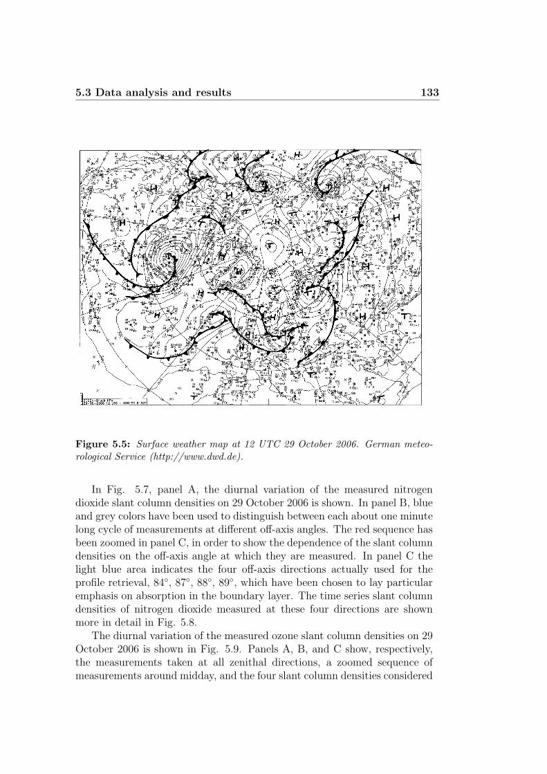
5.3 Data analysis and results 133
Figure 5.5: Surface weather map at 12 UTC 29 October 2006. German meteo-rological Service (http://www.dwd.de).
In Fig. 5.7, panel A, the diurnal variation of the measured nitrogendioxide slant column densities on 29 October 2006 is shown. In panel B, blueand grey colors have been used to distinguish between each about one minutelong cycle of measurements at different off-axis angles. The red sequence hasbeen zoomed in panel C, in order to show the dependence of the slant columndensities on the off-axis angle at which they are measured. In panel C thelight blue area indicates the four off-axis directions actually used for theprofile retrieval, 84, 87, 88, 89, which have been chosen to lay particularemphasis on absorption in the boundary layer. The time series slant columndensities of nitrogen dioxide measured at these four directions are shownmore in detail in Fig. 5.8.
The diurnal variation of the measured ozone slant column densities on 29October 2006 is shown in Fig. 5.9. Panels A, B, and C show, respectively,the measurements taken at all zenithal directions, a zoomed sequence ofmeasurements around midday, and the four slant column densities considered

134 5. NO2 and O3 profiles in the boundary layer
Figure 5.6: 500 hPa weather map at 12 UTC 29 October 2006. German meteo-rological Service (http://www.dwd.de).
in the profile retrieval.
The ligth path for the MAX-DOAS geometry is enhanced in the loweratmosphere compared to zenith sky measurements (see chapter 2, Fig. 2.1).In particular, for the measurements at the four off-axis angles 84, 87, 88,and 89 described here, the photon path is affected by multiple scatteringeffects which necessitate comparison of the measured slant column densitieswith model calculations in order to gain vertical column densities and pro-file information of the absorbers. When modelling the radiative transfer inthe atmosphere, a number of parameters has to be set to realistic values.The most important ones are the viewing geometry, the position of the sun,wavelength, and the vertical profiles of absorbers, pressure and temperature.

5.3 Data analysis and results 135
Figure 5.7: MAX-DOAS NO2 slant column densities measured at Castel Porzianoon 29 October 2006. A: The whole ensemble of measurements taken at the az-imuthal direction of 115 and at a sequence of twelve off-Axis angles (OA) re-peated from 8 a.m. to 4 p.m. (local time). B: the same as in A, every sequenceof measurement being represented by blue and grey colors. The red color sequencehas been zoomed in panel C. C: the sequence of nine OA measurements (60-89)around 10:35 local time, the interval considered for the inversion being displayed(light blue area).
However, the atmospheric aerosol loading also has an impact on the results.

136 5. NO2 and O3 profiles in the boundary layer
Figure 5.8: MAX-DOAS NO2 slant column densities measured at Castel Porzianoon 29 October 2006. Only the four off-axis measurements considered for the in-version have been displayed, corresponding to 84, 87, 88, and 89.
5.3.3 AMF calculation and aerosol setting
The output of the DOAS analysis are the slant column densities. To convertthese into vertical column densities, which are independent of the viewinggeometry, air mass factors (AMFs) have to be calculated with a radiativetransfer model. The AMF is defined as the ratio of the slant to the verticalcolumn density of a given absorber (see Eq. 2.5, chapter 2). In the presentstudy, AMFs were computed by the radiative transfer model PROMSAR (seechapter 3). This model is able to calculate the air mass factor of selected tracegases taking into account multiple scattering and different aerosol scenarios.Both these aspects greatly affect the light paths in the lowest atmosphereand have to be considered in the analysis of MAX-DOAS measurements.
The length of the light path through the atmosphere and thus the ob-served optical depth of a trace gas will depend on the amount and opticalproperties of aerosol particles present in the atmosphere. In general, in-creasing the aerosol extinction reduces the light path for the lower viewingdirections but has litte impact on the zenith-like directions, thereby reduc-ing the difference in tropospheric absorption path for the different viewingdirections.Assuming the properties of atmospheric aerosols and therefore the light pathdistribution is known, it is possible to retrieve information on the vertical pro-file of atmospheric trace gases by measuring their optical depth at differentviewing directions. However, a complementary way of retrieving informationon the state of the atmosphere is to use measurements of the optical depths

5.3 Data analysis and results 137
Figure 5.9: MAX-DOAS O3 slant column densities measured at Castel Porzianoon 29 October 2006. A: The whole ensemble of measurements taken at the az-imuthal direction of 115 and at a sequence of twelve OA repeated from 8 a.m. to4 p.m. (local time). B: the sequence of nine OA measurements (60-89) at about12 local time, the interval considered for the inversion being displayed (light bluearea). C: the four OA measurements considered for the inversion (84, 87, 88,89).
along different lines of sight for an absorber with known vertical profile. Thisprovides information on the vertical distribution and optical properties of at-mospheric aerosols [68]. Recent studies (e.g. [69]) illustrate that the oxygendimer O4 is ideally suited for this approach. The concentration of O4 is pro-

138 5. NO2 and O3 profiles in the boundary layer
portional to the square of the O2 concentration and therefore exponentiallydecreasing with altitude with a scale height of approximately 4 km. Sincethe majority of O4 is located close to the surface, the optical depth of O4 isvery sensitive to changes in the light path distribution at low altitudes.Deriving the aerosol properties from the O4 measurements consists in sim-ulating with a radiative transfer model the vertical columns of O4 varyingthe aerosol extinction profile and composition, and comparing the simulatedcolumns to the measured ones until closure for all lines of sight has beenreached.
O4 has some absorption bands in the UV/visible spectral region. How-ever, during the measurement campaign at Castel Porziano, we used twospectral intervals optimised for NO2 and ozone retrieval which do not in-clude useful O4 absorption bands. For that reason, within the present study,we didn’t use the above described criterion to identify the aerosol scenarioneeded to perform the radiative transfer simulations and calculate the AMFsof the trace gases under investigation. We founded our criterion on the as-sumptions made about the origin of air masses arriving over Castel Porzianoon 29 October 2006, based on the wind direction data analysis (see section5.3.1) and on backward trajectory calculations, which will be discussed insection 5.3.4. Taking into account that the prevailing wind direction on29 October was from the north-east (the direction of Rome), the AMFshave been simulated using an urban aerosol extinction profile taken from theMODTRAN library, with visibility of 5 km and 23 km in the boundary layerand in the free troposphere, respectively. In the stratosphere, the aerosolloading was that of a background aerosol setting and a cloud-free model wasassumed.
In Fig. 5.10 the AMFs (actually box-AMFs, see chapter 2) at 440 nm andSZA=50, 80 are shown. As expected, the largest values of AMFs are foundfor the largest off-axis angles and the lowest atmospheric layers, in agreementwith what discussed in chapter 2. These strongly extended absorption pathsin the lowest few kilometers cause the high sensitivity of MAX-DOAS obser-vations for the boundary layer. For smaller off-axis angles, the box-AMFsfor the lowest atmospheric layers decrease monotonously. For the highestatmospheric layers, the box-AMF converges towards the geometrical approx-imation for a solar zenith angle of 50 (1/cos(50)∼ 1.56) and a solar zenithangle of 80 (1/cos(80)∼ 5.76), as shown in Fig. 5.11.
5.3.4 The retrieval of NO2 and ozone vertical profiles
The retrieval theory presented in chapter 4, in particular the Chahine algo-rithm, can be applied to derive the vertical profile of nitrogen dioxide and

5.3 Data analysis and results 139
Figure 5.10: Box-AMFs for 440 nm as a function of altitude. The of-axis anglesincrease from 0 (zenith) to 89. (top) SZA=50, (bottom) SZA=80.
ozone in the boundary layer from the measured slant column densities, shownin Figs. 5.8 and 5.9 (bottom).
While the vertical profile of a trace gas is a continuous function in the realatmosphere, it has to be approximated by a discrete function and, therefore,sampled at a finite number of points in the retrieval process. The verticalresolution of retrieved profiles depends on the number of viewing directions,SZA, aerosol loading and surface albedo but is in the order of 3 to 5 layersfor the lower troposphere [70]. This means that, depending on measurementconditions, between 3 and 5 pieces of information can be retrieved.Figure 5.12 shows the vertical profiles of nitrogen dioxide and ozone resultingfrom application of the Chahine inversion algorithm to the measured SCDs.NO2 and ozone concentrations in the lower troposphere are driven by a seriesof factors, such as the presence of sources and sinks, the chemical transfor-mations and the transport. All these factors lead to a strong variability ofsuch species both in space and time. For non urban sites typical values ofNO2 and ozone in the boundary layer range from 1 to 20 ppb and from 10 to

140 5. NO2 and O3 profiles in the boundary layer
Figure 5.11: Box-AMFs for 440 nm as a function of altitude (logarithmic scale).The off-axis angles increase from 0 (zenith) to 89. (top) SZA=50, (bottom)SZA=80.
100 ppb, respectively (see e.g., [71],[72], and [5]). Since it was not possible touse in this study climatological mean profiles as the initial guess, as it wouldbe appropriate, the initial guess profiles used were that NO2 had a concen-tration exponentially decreasing with altitude (a constant mixing ratio withaltitude) and ozone has a homogeneous constant concentration with altitude.The vertical profiles have been retrieved at four altitude levels, 50 m, 350m, 650 m, and 1150 m. The first level was set to 50 m for two main rea-sons. First, this altitude was deduced from simple geometric considerationsbased on the greatest off-axis angle used (89) and the PROMSAR-estimatedlength of the path (∼3 km) the photons cover, on average, when collected atthis line of sight. Second, this choice prevents light reflected by the groundor obstacles from entering the field of view of the instrument. The otherlevels correspond to the heights for which averaging kernels show the high-est retrieval sensitivity. The averaging kernels (see chapter 4 for the formaltreatment) define the sensitivity of the retrieved profiles to changes of the

5.3 Data analysis and results 141
Figure 5.12: NO2 (top) and O3 (bottom) concentration profiles and vertical col-umn densities in the boundary layer deduced from a set a MAX-DOAS measure-ments taken at four off-axis angles (84, 87, 88, 89) and at the azimuthal di-rection of 115. Measurements have been carried out at the Presidential Estate ofCastel Porziano (20 km South-West of Rome) on 29 October 2006.
real atmospheric profiles; in other words they demonstrate how much the re-trieval algorithm is able to reproduce a given input profile. For example, Fig.5.13 illustrates the capability of the retrieval algorithm in reproducing four

142 5. NO2 and O3 profiles in the boundary layer
input profiles (the dashed red lines) with the gas concentrated, respectively,at 50 m, 350 m, 650 m, and 1150 m (the four altitudes of the retrieval). Solidred lines represent the retrieved profiles. The averaging kernels correspond-ing to the four levels of the retrieval are shown in Fig. 5.14. Figures 5.13 and
Figure 5.13: The profiles obtained through inversion of the slant column amountssimulated using different input profiles have been compared with the input profilesthemselves. From this analysis, the averaging kernels are calculated.
5.14 illustrate that at most three pieces of information can be retrieved. Es-sentially no information (other than that contained in the first guess profile),in fact, was found to come from the upper level (1150 m) meaning that theretrieval algorithm is not able to detect changes in the true profile at 1150m. Concerning the other levels, the averaging kernel at 50 m shows thatthe retrieval algorithm is able to detect close to 55% of change in the trueprofile, the averaging kernel at 350 m close to 70%, and the averaging kernelat 650 m close to 20%. We can conlude, therefore, that the resolution ofthe retrieved profiles is of 3 layers between 0 to 2 km. Finally, the averagingkernels shown in Figs. 5.13 and 5.14 reveal a better sensitivity of the profileretrieval at 350 m. The maxima of the weighting functions are indicators forthe altitude from which we obtain most of the information for a given line ofsight.

5.3 Data analysis and results 143
Figure 5.14: Averaging kernels.
Considerations about the retrieved profiles and validation
Figure 5.12 shows the retrieved vertical profile of NO2 and O3 and theirvertical column density from 0 to 2 km, calculated by integrating the con-centration values from the lower to the upper level of retrieval. The verticalcolumns reach maximum values of about 6 · 1015 molecules/cm2 for nitro-gen dioxide and 1.5 · 1017 molecules/cm2 for ozone. Moreover, the verticalcolumns of NO2 and O3 are anti-correlated, which is indicative of their dailyphotochemical cycle. NO2, in fact, is known to produce ozone after somedelay and it is not surprising that the ozone amount is fairly uniform fromabout 12:20 to 14:20. As for the spike in ozone at about 13:05 and the min-imum at 12:55, we can exclude any artefact and hypothesize a correlationwith transport.
Comparing the vertical columns in the boundary layer with similar in-dependent quantities can be useful for checking the correctness of the re-trieval algorithm. As for nitrogen dioxide, for example, we have comparedthe vertical column shown in Fig. 5.12 (top) with the tropospheric verticalcolumn obtained from satellite observations. In particular, we refer to themeasurements carried out by the Ozone Monitoring Instrument (OMI) spec-trometer ([73], [74]), a Dutch-Finnish monitoring instrument that flies onthe Earth Observing System (EOS) NASA’s Aura satellite, launched in Jan-uary 2004. OMI is a nadir viewing, near-UV and visible spectrograph whichdraws heavily on European experience in atmospheric research instrumentssuch as GOME (flying on ERS-2), SCIAMACHY and GOMOS (both flyingon ENVISAT). OMI’s nadir spatial resolution ranges from 13 × 24 km to 24

144 5. NO2 and O3 profiles in the boundary layer
× 48 km , depending on the instrument’s operating mode.Figure 5.15 shows the mean tropospheric vertical columns of nitrogen diox-ide from OMI instrument, carried out on 29 October 2006. Such columns
Figure 5.15: NO2 tropospheric columns from OMI on 29 October 2006.
range from about 6 · 1015 molecules/cm2 to about 10 · 1015 molecules/cm2. Agood agreement is therefore found with the vertical column amounts in theboundary layer deduced from MAX-DOAS measurements.
In order to focus our discussion on nitrogen dioxide we analyse Fig. 5.16,which shows the daily evolution of the NO2 vertical profile at 50 m, 350 m,and 650 m. Also error bars are shown in Fig. 5.16, calculated accordingto the analysis of averaging kernels discussed previously. Figures 5.16 and5.12 show that the highest NO2 values are found at 350 m (with a peak ofabout 5 ppb at 10:45), although the initial guess profile of nitrogen dioxidehad a concentration exponentially decreasing with altitude. This suggeststhat NO2 was probably transported over the Castel Porziano Estate from re-mote sources, rather than local ones. Because of the absence of independentin-situ measurements using e.g. balloon and aircraft-borne instruments, areal validation of these retrieved profiles was not allowed. Nevertheless, we

5.3 Data analysis and results 145
Figure 5.16: Diurnal evolution of nitrogen dioxide vertical profile at differentaltitude levels, as deduced by means of the retrieval inversion algorithm.
performed a set of simulations with the Hybrid Single Particle LagrangianIntegrated Trajectory (HYSPLIT) model, initialized with synoptic meteoro-logical fields produced by the National Weather Service’s National Centers

146 5. NO2 and O3 profiles in the boundary layer
for Environmental Prediction (NCEP) and archived at the NOAA Air Re-sources Laboratory (GDAS1 archive), in order to calculate the backwardtrajectories of the polluted air masses arriving over the Castel Porziano areaduring the day under examination.Figure 5.17 shows the backward trajectories ending at 9 UTC (10 a.m. localtime) computed at three altitude levels (red: 50 m, blue: 250 m, green: 500m., a.s.l.) on 29 October 2006. It can be seen that the prevailing direction
Figure 5.17: Trajectories ending at Castel Porziano on 29 October 2006. CastelPorziano (41.74 N, 12.40 E) is indicated by the star symbol. Red, blue and greenlines indicate, respectively, back trajectories ending exactly at Castel Porziano atdifferent altitude levels (red: 50 m, blue: 250 m, green: 500 m). Trajectorieshave been computed with the Hybrid Single Particle Lagrangian Integrated Trajec-tory (HYSPLIT) model, provided by the NOAA Air Resources Laboratory. TheCiampino airport (41.80 N, 12.60 E) is also indicated.

5.3 Data analysis and results 147
of air masses resulting from the HYSPLIT model was the North-East di-rection, which corresponds to Ciampino Airport (41.80 N, 12.60 E) and theareas of heavy traffic surrounding the city of Rome. It can be noticed thatthe air mass coming from the Ciampino airport has been sampled at CastelPorziano less than two hours later, a time interval which is shorter than theNO2 lifetime [5].Trajectories ending at 8 UTC and 10 UTC were also computed (not shownhere), and turned out to be very similar to those ending at 9 UTC. Figure5.18 also shows the backward trajectories ending at 9 UTC computed at threedifferent altitude levels (red: 50 m, blue: 250 m, green: 500 m., a.s.l.) on 25,26, 27, 28, 29, and 30 October 2006. The mean wind data recorded at thePratica di Mare station and shown in Fig. 5.4 confirme that the prevailingwind direction measured on 29 October 2006 was from North-East.
Retrieval method performances
The retrieval method performances can be evaluated, for example, by com-parison between the measured and recalculated (i.e. simulated) slant columndensities for the different off-axis directions. Figure 5.19 shows the agreementbetween the observed and recalculated NO2 SCDs at 84, 87, 88, and 89.The observed SCDs are directly obtained from MAX-DOAS observations andrecalculated SCDs are the model calculated values deduced from retrievedvertical profiles for the day under study. The fitting is good, with percentdifferences displayed in Fig. 5.20.

148 5. NO2 and O3 profiles in the boundary layer
Figure 5.18: Trajectories ending at Castel Porziano on 25, 26, 27, 28, 29, and 30October 2006. In every panel Castel Porziano (41.74 N, 12.40 E) is indicated bythe star symbol. Red, blue and green lines indicate, respectively, back trajectoriesending exactly at Castel Porziano at different altitude levels (red: 50 m, blue: 250m, green: 500 m). Trajectories have been computed with the Hybrid Single ParticleLagrangian Integrated Trajectory (HYSPLIT) model, provided by the NOAA AirResources Laboratory.

5.3 Data analysis and results 149
Figure 5.19: Measured and recalculated nitrogen dioxide slant column densitiesat 84, 87, 88, and 89.
Figure 5.20: Percent errors distribution of the measured and simulated slantcolumn densities shown in Fig. 5.19.

150 5. NO2 and O3 profiles in the boundary layer

Conclusions
A recent development in ground-based remote sensing of atmospheric con-situents by UV/visible absorption measurements of scattered light is the si-multaneous use of several directions in addition to the traditional zenith-skypointing: this technique is referred to as Multiple AXis Differential OpticalAbsorption Spectroscopy (MAX-DOAS).
As well as zenith-looking DOAS, Multiple AXis DOAS can detect thepresence of a trace gas in terms of its integrated concentration over an at-mospheric path, the so called slant column density. A special feature of theMAX-DOAS technique, however, are the off-axis viewing directions close tothe horizon, showing stronger signal of tropospheric absorbers than zenith-sky observations, particularly sensitive to stratospheric absorbers. In thisway, the MAX-DOAS represents a new approach to the problem of measur-ing tropospheric concentrations of some atmospheric trace gases by observingtheir absorption in UV/visible scattered sunlight. Depending on troposphericvisibility, the light path in the lower atmospheric layers can become very longusing the MAX-DOAS configuration and increases as the viewing directionapproaches the horizon. Information from the different lines of sight can beused to derive the vertical profile of the absorbers of interest, in the tropo-sphere and even in the boundary layer.
Retrieval of profile information from the slant column density of a giventrace gas couldn’t be performed without (1) accurately modelling of the lightpath with radiative transfer models (RTMs) and (2) application of effectiveinversion techniques.
The ability to properly interpret UV/visible absorption measurements ofatmospheric constituents using scattered light, in fact, depends crucially onhow well the optical path of light collected by the system is understood. Thisknowledge is essential to convert the slant column density of the absorber,which can be derived from the absorption measurements, into a vertical col-umn density (the concentration of the absorber integrated along the vertical),with the help of the so-called Air Mass Factor (AMF). This factor is definedas the ratio of the slant column density to the vertical column density and

152 Conclusions
can be used to quantify the enhancement of the light path length within theabsorber layers.In the case of zenith-sky DOAS measurements, calculations of the air massfactor have been made using “simple” single scattering radiative transfermodels. For measurements with the telescope pointing toward the horizon,however, multiple scattering has to be taken into account. In addition, thefull treatment of atmospheric sphericity in the radiative transfer includingrefraction turns out to be necessary at low sun.
A useful approach to take into account such aspects and, moreover, todeal with all physical parameters affecting the light paths, to support allDOAS geometries, and treat multiple scattering with varying phase func-tions involved, is the Monte Carlo approach. The development and applica-tion of the Monte Carlo radiative transfer model PROMSAR (PROcessing ofMulti-Scattered Atmospheric Radiation) is a major concern of the researchpresented in this thesis.Besides calculating the air mass factor, which is the fundamental output forthe interpretation of remote sensing measurements, the PROMSAR modelalso calculates the atmospheric transmittance, the solar direct and diffuse ir-randiance and the radiance, for a detector with assigned central coordinates,diameter, direction cosines of the normal to the detector surface, line of sightand field of view. As a validation, the radiometric quantities and the air massfactors calculated by the PROMSAR model have been extensively comparedwith the same quantities computed by other radiative transfer models: theMODTRAN code, as for the transmittance, irradiance and radiance calcu-lations, and eigth different state-of-the-art RTMs from seven internationalresearch groups, as for the AMF and radiance calculations.
In order to derive the vertical concentration profile of a trace gas from itsslant column density, the AMF is only one part in the quantitative retrievalprocess. The other indispensable requirement is a robust approach to solvefor the equation system composed from the AMFs, the measurements and theunknown concentrations: that is, an inversion method. Within the presentstudy, after dealing with the retrieval theory in general, mainly following thework of Rodgers, the Chahine relaxation method has been presented. Thismethod was successfully used in the past by several authors to estimate theprofile information contained in zenith-sky DOAS measurements at differentsolar zenith angles using ground-based instruments. The vertical resolutionof such profiles was, however, relatively low (from 5 to 10 km) and infor-mation was limited mainly to the stratospheric part of the profile. Withinthe study presented in this thesis, the Chahine inversion method has beenmodified so as to be applied for inversion of ground-based Multiple AXisDOAS measurements. The aim is the retrieval of the vertical profile of the

Conclusions 153
trace gases of interest in the lower troposphere and boundary layer, which ispossible taking advantage of the variation of the slant column measurementswith the off-axis angle instead of variation with the solar zenith angle, as inthe case of zenith-sky measurements.
One day of measurements carried out at Castel Porziano (41.74 N, 12.40E), near Rome, in October 2006 using a MAX-DOAS instrument have been,finally, presented. The amount of profile information that can be retrievedfrom such measurements, in particular, is investigated for the trace gasesNO2 and, to a lesser degree, for ozone. Even if uncertainties remain in theretrieved profiles mainly due to the lack of independent observations and ofa climatology for comparison, the results indicate that the pollutants areprobably transported over Castel Porziano from remote sources, mainly theCiampino airport and the heavy traffic area surrounding the city of Rome.This hypotesis finds confirmation in the backward trajectory calculationscarried out with the HYSPLIT model and the wind data recorded at thePratica di Mare meteorological station, located near the area under study.
In summary, ground-based Multiple AXis Differential Optical AbsorptionSpectroscopy, combined with appropriate radiative transfer models and in-version techniques, is a promising tool for atmospheric studies in the lowertroposphere and boundary layer, including the retrieval of profile informa-tion with a good degree of vertical resolution. This thesis has presented anapplication of this powerful comprehensive tool for the study of a preservednatural Mediterranean area where pollution can only be transported fromremote sources.Application of this tool in densely populated or industrial areas is beginningto look particularly fruitful and represents an important subject for futureworks. In these areas the most important source of NO2 are anthropogenicemissions; since all NO2 emissions affect the boundary layer directly, themonitoring of the NO2 levels in the boundary layer is getting more and moreimportant. In the troposphere NO2 is an important trace gas since its photo-chemistry is also involved in the production of tropospheric ozone. Thus themonitoring of NO2 concentrations in these areas is necessary because ozoneand nitrogen dioxide itself are harmful species affecting both human healthand the growth of vegetation. To understand the NO2 (actually, NOx) andozone chemistry in more detail not only the concentrations at ground butalso the acquisition of the vertical distribution of the trace gases is necessary.Thus a tool to resolve the vertical profile information is really important.A MAX-DOAS instrument, together with a sophisticated radiative transfermodel and a retrieval method are a tool with promising applications.

154 Conclusions

Appendix
Urban and free tropospheric NO2 and O3
chemistry
In this Appendix, some chemical reaction pathways primarily involving ni-trogen dioxide and ozone are described for the free troposphere and urbanregions. The omitted reactions can be found, for example, in [5] and [11].
Photostationary-state ozone concentration
In the background troposphere, the ozone (O3) mixing ratio is determinedprimarily by a set of three reactions involving itself, nitric oxide (NO), andnitrogen dioxide (NO2). These reactions are:
NO +O3 −→ NO2 +O2 (1)
NO2 + hν −→ NO +O λ < 420 nm (2)
O +O2 −→ O3 (3)
where hν implies a photon of solar radiation and λ is the wavelength of theradiation. Background tropospheric, mixing ratios of O3 (20 to 60 ppbv)are much higher than those of NO (1 to 60 pptv) or NO2 (5 to 70 pptv).Because the mixing ratio of NO is much lower than is that of O3, reaction 1does not deplete ozone during the day or night in background troposphericair. In urban air reaction 1 can deplete local ozone at night because NOmixing ratios at night may exceed those of O3.
If k1 (cm3·molecule−1·s−1) is the rate coefficient of reaction 1 and J (s−1)is the photolysis rate coefficient of reaction 2, the volume mixing ratio ofozone can be calculated from these two reactions as
χO3 =J
Ndk1
· χNO2
χNO
(4)

156 Appendix
where χ is volume mixing ratio (molecule of gas per molecule of dry air)and Nd is the concentration of dry air (molecules of dry air per cubic cen-timeter). This equation is called the photostationary-state relationship.The equation does not state that ozone is affected by only NO and NO2.Indeed, other reactions affect ozone, including ozone photolysis. Instead,Eq. 4 predicts a relationship among NO, NO2, and O3. If two of the threeconcentrations are known, the third can be found from the equation.
Two important reactions aside from Eqs. 1-3 that affect ozone are:
O3 + hν −→ O2 +O(1D) λ < 310 nm (5)
O3 + hν −→ O2 +O λ > 310 nm (6)
where O(1D) is the excited atomic oxygen. In the free troposphere, the lif-time of ozone against destruction by these reactions are about 0.7 and 14 h,respectively. The lifetime of ozone against destruction by NO is in generallonger than lifetime of ozone against photolysis. Thus, in the daytime freetroposphere, photolysis destroys ozone faster than does reaction with NO.When the ozone concentration changes due to photolysis, the χNO2/χNO
ratio in Eq. 4 changes to adapt to the new ozone concentration.The photostationary-state relationship in Eq. 4 is useful for free tropo-
spheric analysis. In urban air, though, the relationship often breaks downbecause reactions of NO with organic gas radicals provide an additional im-potant source of NO2, not included in Eq. 4. When organic-radical con-centrations are large, as they are during the morning in urban air, thephotostationary-state relationship does not hold. In afternoon, though, or-ganic gas concentrations in urban air decrease, and the relationship holdsbetter.
When excited atomic oxygen forms, as in Eq. 5, it rapidly produces O by
O(1D)M O (7)
and O rapily produces O3 by Eq. 3. The reactions 3 and 5-7 cycle oxygenatoms quickly among among O(1D), O, and O3. Losses of O from the cycle,such as from conversion of NO to NO2 by Eq. 1, are slower than are transfersof O within the cycle.
Daytime removal of nitrogen oxides
During the day, NO2 is removed slowly from the photostationary-state cycleby the reaction
NO2 +OHM−→ HNO3 (8)

Appendix 157
where M represents any other molecule which, while not directly involved inthe chemical reaction, can carry away excess energy formed in the reaction.Because molecular oxygen O2 and nitrogen N2 together make up more than99 percent of the gas molecules in the air today, M is most likely to be O2
or N2. Although HNO3 photolyzes back to NO2 + OH (for λ < 335 nm),its lifetime against photolysis is 15 to 80 days, depending on the day of theyear and the latitude. Because this lifetime is faily long, HNO3 serves as sinkfor nitrogen oxides NOx (= NO + NO2) in the short term. In addition,because HNO3 is soluble, much of it dissolves in cloud drops or aerosol par-ticles before it photolyzes back to NO2.Reaction 8 requires the presence of the hydroxyl radical (OH), an oxidiz-ing agent that decomposes (scavenges) many gases. Given enough time, OHbreaks down every organic gas and most inorganic gases in the air. The glob-ally averaged tropospheric OH concentration is about 8×10⁵ molecules cm−3.Its daytime concentration in the clean free troposphere usually ranges from2×105 to 3×10⁶ molecules cm−3. In urban air, OH concentration typicallyranges from 1×10⁶ to 1×10⁷ molecules cm−3.The primary free-tropospheric source of OH is the pathway
O3 + hν −→ O2 +O(1D) λ < 310 nm (9)
O(1D) +H2O −→ 2OH (10)
Most of the O(1D) atoms produced by reaction 9 dissipate their excess energyas heat and eventually recombine with O2 to form O3, which is a null cycle(i.e., it has no net chemical effects). However, a small fraction (∼0.01) of theO(1D) atoms reacts with water vapour to form two hydroxyl radicals as inreaction 10. Thus, the OH concentrations in the free troposphere depend onozone and water vapour contents. In the upper troposphere, H2O is scarce,limiting the ability of reaction 10 to produce OH. Minor sources of OH inthe free troposphere are photolysis of gases, some of which are produced byOH itself. For example, nitrous acid (HONO), produced during the dayby the reaction of NO with OH, rapidly photolyzes to produce OH and NO(λ < 400 nm). HONO concentrations are high only during the early morningbecause the photolysis rate increases as sunlight becomes more intense duringthe day. During the night, HONO is not produced from gas-phase reactions,since OH, required for its production, is absent at night. HONO is producedfrom gas-particle reactions and emitted from vehicles during day and night.
Once formed, the OH radical is a powerful oxidant that reacts quickly(the lifetime of OH in the atmosphere is only about one second) with anumber of atmospheric pollutants: NO2 to form HNO3 (reaction 8), CO toform CO2, H2S to form SO2, SO2 to form H2SO4, CH2O to form CO, and so

158 Appendix
on. Because of its pivotal role in transforming a large number of troposphericgases (many of which are major pollutants) into their oxidized forms, OH hasbeen referred to as the “atmopshere’s detergent”.
Nighttime nitrogen chemistry
During the night, reaction 2 shuts off, eliminating the major chemical sourcesof O and NO. Because O is necessary for the formation of ozone, ozoneproduction also shuts down at night. Thus, at night, neither O and NO, norO3 is produced chemically. If NO is emitted at night, it destroys ozone byreaction 1. Because NO2 photolysis shuts off at night, NO2 becomes avalilaleto produce NO3, N2O5, and HNO3 at night by the sequence
NO2 +O3 −→ NO3 +O2 (11)
NO2 +NO3
M N2O5 (12)
N2O5 +H2O −→ 2HNO3 (13)
Reaction 11 occurs during the day as well, but, during the day, it is less im-portant than NO+O3, an the NO3 produced from the reaction is photolyzedalmost immediately by solar radiation
NO3 + hν −→ NO +O2 (14)
and
NO3 + hν −→ NO2 +O (15)
Although NO3 is much less reactive than OH, at night it is present in higherconcentrations than OH is during the day.Reaction 12 is a reversible reaction. At high temperature, such as during theday, the reverse reaction occurs within seconds. At low temperature, such asat night, is occurs within hours or days or even months.Reaction 13 is an heterogeneous reaction, occurring on aerosol or hydrome-teor particle surfaces.
Ozone production in the background troposphere: anair pollution problem
Ozone plays a key but dichotomous role in the atmosphere. In both thetroposphere and the stratosphere it is a key reactant. In the stratosphereozone absorbs dangerous UV radiation, thereby protecting life on Earth. In
Appendix 159
the troposphere it is a potent pollutant, toxic to humans and vegetation dueto its oxidizing power on biological tissues, but it is also the source of the“detergent” OH.Besided being involved in the photostationary-state relationship (4), O3 isproduced in the troposphere from the oxidation of the carbon monoxide(CO), methane (CH4) and certain nonmethane organic gases by OH in thepresence of NOx. In densely populated regions with high emissions of NOx
and hydrocarbons, rapid O3 production can take place and results in a surfaceair pollution problem.CO produces ozone by
CO +OH −→ CO2 +H (16)
H +O2 −→ HO2 (17)
NO +HO2 −→ NO2 +OH (18)
NO2 + hν −→ NO +O λ < 420 nm (19)
O +O2
M O3 (20)
Methane, is the most abundant organic gas in the Earth’s atmosphere. Itsfree-tropospheric lifetime against chemical destruction is 8 to 12 years. Thislong lifetime has enabled it to mix uniformly up to the tropopause. Abovethe tropopause, its mixing ratio decreases. The methane oxidation sequenceproducing ozone is
CH4 +OH −→ CH3 +H2O (21)
CH3 +O2 −→ CH3O2 (22)
NO + CH3O2 −→ NO2 + CH3O (23)
NO2 + hν −→ NO +O λ < 420 nm (24)
O +O2
M O3 (25)
Note that in the stratosphere, reaction 21 is an important source of watervapour. As with reaction 17, reaction 22 is fast.
Urban photochemistry and air pollution
Photochemical smog results from the emission of organic gases in the pres-ence of sunlight. It differs from background air in two ways. First, mixingratios of nitrogen oxides and organic gases are higher in polluted air than in
160 Appendix
background air, causing ozone levels to be higher in urban air than in thebackground. Second, photochemical smog contains higher concentrations ofhigh molecular weight organic gases, particularly aromatic gases, than doesbackground air. Because such gases break down quickly in urban air, mostare unable to survive transport to background troposphere.
Photochemical smog involves reactions among nitrogen oxides (NOx =NO + NO2) and reactive organic gases (ROGs, total organic gases minusmethane) in the presence of sunlight. The most recognized gas-phase by-product of smog reactions is ozone because has harmful health effects and isan indicator of the presence of other pollutants.
On a typical morning, NO and ROGs are emitted by traffic, power plants,and other combustion sources. Emitted pollutants are primary pollutants.ROGs are oxidized to organic peroxy radicals, denoted by RO2, which reactwith NO to form NO2. Pre-existing ozone also convert NO to NO2. Sunlightthen breaks down NO2 to NO and O. Finally, O reacts with molecular oxygento form ozone. The basic reaction sequence is thus:
NO +RO2 −→ NO2 +RO (26)
NO +O3 −→ NO2 +O2 (27)
NO2 + hν −→ NO +O λ < 420 nm (28)
O +O2 +M −→ O3 +M (29)
Pollutants, like ozone, that form chemically or physiscally in the air aresecondary pollutants.
Because RO2 competes with O3 to convert NO to NO2 in urban air, andbecause the photostationary state relationship is based on the assumptionthat only O3 converts NO to NO2, the photostationary relationship isusually not valid in urban air. In the afternoon, the relationship holdsbetter than it does in the morning because RO2 mixing ratios are lower inthe afternoon than in the morning.

Bibliography
[1] Brasseur, G. P., J. J. Orlando, G. S. Tyndall (eds.), Atmosphericchemistry and global change, Oxford University Press, New York,1999.
[2] Stull, R. B., An introduction to boundary layer meteorology,Kluwer Academic Publishers, Dordrecht, 1988.
[3] Solomon, S., R. W. Portmann, R. W. Sanders, J. S. Daniel, W. Madsen,B. Bartram, E. G. Dutton, On the role of nitrogen dioxide in the ab-sorption of solar radiation, J. Geophys. Res., 104 (D10), 12047-12058,1999.
[4] Wallace, J. M., P. V. Hobbs, Atmospheric Science, an introductorysurvey, Academic Press, San Diego, 1977.
[5] Hobbs P. V., Introduction to atmospheric chemistry, CambridgeUniversity Press, 262 pages, 2000.
[6] Rayleigh, L., On the light from the sky, its polarization and colour, Phil.Mag., 41, 107-20, 1871.
[7] Mie, G., Optics in turbid media, Ann. Phys., 25, 377-445, 1908.
[8] Waggoner, A. P., R. E. Weiss, N. C. Ahlquist, D. S. Covert, S. Will,R. J. Charlson, Optical characteristics of atmospheric aerosols, Atmos.Environ., 15, 1891-1909, 1981.
[9] Cass, G. R., On the relationship between sulfate air quality and visibilitywith examples in Los Angeles, Atmos. Environ., 13, 1069-1084, 1979.
[10] Tang, I. N., W. T. Womg, H. R. Munkelwitz, The relative importanceof atmospheric sulfates and nitrates in visibility reduction, Atmos. En-viron., 15, 2463-71, 1981.
161

162 BIBLIOGRAPHY
[11] Jacobson, M. Z., Fundamentals of atmospheric modeling, Cam-bridge University Press, 2005.
[12] Schneider, W., G. K. Moortgat, G. S. Tyndall, J. P. Burrows, Absorptioncross-sections of NO2 in the UV and visible region (200-700 nm) at 298K, J. Photochem. Photobiol. A: Chem., 40, 195-217, 1987.
[13] Plane, J. M. C., N. Smith, Atmospheric monitoring by differential op-tical absorption spectroscopy, in Spectroscopy in EnvironmentalSciences, edited by Hester, R. E. and Clark, R. J. H., John Wiley, NewYork, 223-262, 1995.
[14] Dobson, G. M. B., D. N. Harrison, Measurements of the amount ofozone in the Earth’s Atmosphere and its Relation to other GeophysicalConditions, Proc. R. Soc. London, 110, 660-693, 1926.
[15] Gotz, P. F. W., A. R. Meetham, G. M. B. Dobson, The Vertical Dis-tribution of Ozone in the Atmosphere, Proc. Roy. Soc., A 145, 416-446,1934.
[16] Davies, J., Correlation Spectroscopy, Analytical Chemistry, 42, 101-112,1970.
[17] Hoff, R., M. Millan, Remote SO2 mass flux measurements usingCOSPEC. JAPCA, 31, 381-384, 1981.
[18] Hoff, R. M., Differential SO2 Column Measurements of the Mt. PinatuboVolcanic Plume, Geophys. Res. Lett., 19, 175-178, 1992.
[19] Platt, U., Differential optical absorption spectroscopy (DOAS),in Air Monitoring by Spectroscopic Techniques, edited by: Sigrist, M.W., Chemical Analysis Series, 127, John Wiley, New York, 1994.
[20] Sanders, R. W., S. Solomon, J. P. Smith, L. Perliski, H. L. Miller, G.H. Mount, J. G. Keys, A. L. Schmeltekopf, Visible and Near-UltravioletSpectroscopy at McMurdo Station Antarctica, 9. Observations of OClOfrom April to October 1991, J. Geophys. Res., 98, D4, 7219-7228, 1993.
[21] Arpaq, K. H., P. V. Johnston, H. L. Miller, R. W. Sanders, S. Solomon,Observations of the stratospheric BrO column over Colorado, 40 N, J.of Geophys. Res., 99, D4, 8175-8181, 1994.
[22] Miller, H. L., A. Weaver, R. W. Sanders, K. Arpag, S. Solomon, Mea-surements of arctic sunrise surface ozone depletion events at Kangerlus-suaq, Greenland (67N, 51W), Tellus, 49B, 496-509, 1997.

BIBLIOGRAPHY 163
[23] Weaver, A., S. Solomon, R. W. Sanders, K. Arpag, H. L. Miller, Atmo-spheric NO3 5. Off-axis measurements at sunrise: Estimates of tropo-spheric NO3 at 40N, J. Geophys. Res., 101, D13, 18605-18612, 1996.
[24] Smith, J., S. Solomon, Atmospheric NO3: 3. Sunrise Disappearance andthe Stratospheric Profile, J. Geophys. Res., 95, D9, 13819-13827, 1990.
[25] Smith, J., S. Solomon, R. Sanders, H. Miller, J. Perliski, J. Keys, A.Schmeltekopf, Atmospheric NO3: 4. Vertical Profiles at Middle and Po-lar Latitudes at Sunrise, J. Geophys. Res., 98, D5, 8983-8989, 1993.
[26] Stutz, J., U. Platt, Numerical Analysis and Estimation of the Statisti-cal Error of Differential Optical Absorption Spectroscopy Measurementswith Least-Squares methods, Appl. Opt., 35, 30, 6041-6053, 1996.
[27] Grainger, J., J. Ring, Anomalous Fraunhofer line profiles, Nature, 193,762, 1962.
[28] Fish, D. J., R. L. Jones, Rotational Raman scattering and the Ringeffect in zenith-sky spectra, Geophys. Res. Lett., 22, 811-814, 1995.
[29] Sioris, C. E., W. F. J. Evans, Filling in of Fraunhofer and gas absorptionlines in sky spectra as caused by rotational Raman scattering, Appl.Opt., 38, 12, 2706-2713, 1999.
[30] Marquard, L., T. Wagner, U. Platt, Improved Air Mass Factor Conceptsfor Scattered Radiation Differential Optical Absorption Spectroscopy ofAtmospheric Species, J. Geophys. Res., 105, 1315-1327, 2000.
[31] Solomon, S., A. L. Schmeltekopf, R. W. Sanders, On the interpretationof zenith sky absorption measurements, J. Geophys. Res., 92, 8311-8319,1987.
[32] Perliski, L. M. S. Solomon, On the evaluation of air mass factors for at-mospheric near ultraviolet and visible absorption spectroscopy, J. Geo-phys. Res., 98, 10363-10374, 1993.
[33] Palazzi, E., A. Petritoli, G. Giovanelli, I. Kostadinov, D. Bortoli, F.Ravegnani, S. S. Sackey, PROMSAR: A backward Monte Carlo sphericalRTM for the analysis of DOAS remote sensing measurements, Adv. SpaceRes., 36(5), 1007-1014, 2005.
[34] Wagner, T., J. P. Burrows, T. Deutschmann, B. Dix, C. von Friedeburg,U. Frieß, F. Hendrick, K.-P. Heue, H. Irie, H. Iwabuchi, Y. Kanaya, J.

164 BIBLIOGRAPHY
Keller, C. A. McLinden, H. Oetjen, E. Palazzi, A. Petritoli, U. Platt,O. Postylyakov, J. Pukite, A. Richter, M. van Roozendael, A. Rozanov,V. Rozanov, R. Sinreich, S. Sanghavi, F. Wittrock, Comparison of Box-Air-Mass-Factors and Radiances for Multiple-Axis Differential OpticalAbsorption Spectroscopy (MAX-DOAS) Geometries calculated from dif-ferent UV/visible Radiative Transfer Models, Atmos. Chem. Phys., 7,1809-1833, 2007.
[35] United States Committee on Extension to the Standard Atmosphere:U.S. Standard Atmosphere, 1976, National Oceanic and Atmosphe-ric Administration, National Aeronautics and Space Administration,United States Air Force, Washington D.C., 1976.
[36] Bogumil, K., J. Orphal, T. Homann, S. Voigt, P. Spietz, O. C. Fleis-chmann, A. Vogel, M. Hartmann, H. Bovensmann, J. Frerik, J. P. Bur-rows, Measurements of Molecular Absorption Spectra with the SCIA-MACHY Pre-Flight Model: Instrument Characterization and ReferenceData for Atmospheric Remote-Sensing in the 230-2380 nm Region, J.Photochem. Photobiol. A., 157, 167-184, 2003.
[37] Lenoble, J. (Editor), Standard Procedures to Compute Atmospheric Ra-diative Transfer in a Scattering Atmosphere - Volume I, InternationalAssociation of Meteorology and Atmospheric Physics (IAMAP), Boul-der, Colorado, USA, 1977.
[38] Fouquart, Y., W. M. Irvine, J. Lenoble (eds.), Standard Procedures toCompute Atmospheric Radiative Transfer in a Scattering Atmosphere -Volume II, International Association of Meteorology and AtmosphericPhysics (IAMAP), Boulder, Colorado, USA, 1980.
[39] Stamnes, K., S-C. Tsay, W. Wiscombe, K. Jayaweera, Numerically Sta-ble Algorithm for Discrete-Ordinate- Method Radiative Transfer in Mul-tiple Scattering and Emitting Layered Media, Appl. Opt.,27(12), 2502-2509, 1988.
[40] Plass, G. N., G. W. Kattawar, Monte Carlo calculations of light scat-tering from clouds, Appl. Opt., 7, 415-419, 1968.
[41] Plass, G. N., G. W. Kattawar, Radiative transfer in an atmosphere-ocean system, Appl. Opt., 8, 455-466, 1969.
[42] Tinet, E., S. Avrillier, J. M. Tualle, Fast semianalytical Monte Carlosimulation for time-resolved light propagation in turbid media, J. Opt.Soc. Am. A, 13, 1903-1915, 1996.
BIBLIOGRAPHY 165
[43] Wehrli, C., Extraterrestrial Solar Spectrum, WMO No. 615, July 1985.(http://rredc.nrel.gov/solar/standards/am0/wehrli1985.html)
[44] Halton, J. H., A Retrospective and Prospective Survey of the MonteCarlo Method, Siam. Rev., 12, 1-63, 1970.
[45] Bielajew, A. F., D. W. O. Rogers, Variance-reduction techniques. In:Jenkins T. M., Nelson W. R., Rindi A. (eds) Monte Carlo transport ofelectrons and photons. Plenum, New York, pp. 407-419, 1988.
[46] Collins, D. G., W. G. Blattner, M. B. Wells, H. G. Horak, BackwardMonte Carlo calculations of the polarization characteristics of the radi-ation emerging from spherical-shell atmospheres, Appl. Opt., 11, 2684-2696, 1972.
[47] Blattner, W. G., H. G. Horak, D. G. Collins, M.B. Wells, Monte Carlostudies of the sky radiation at twilight, Appl. Optics, 13(3), 534.547,1974.
[48] Berk, A., L. S. Berstein, D.C Robertson, MODTRAN: A ModerateResolution Model of LOWTRAN7, Final Report, GL-TR-0122, AFGL,Hanscom AFB, Maryland, 42 pages, 1989.
[49] Henyey L. C., J. L. Greenstein, Diffuse radiation in the galaxy, Astro-phys. J., 93, 70-83, 1941.
[50] Liou, K. N., An Introduction to atmospheric radiation, Amster-dam, Academic Press, 2002.
[51] Anderson, G. P., J. Wong, J. H Chetwynd, MODTRAN3: An Updateon Recent Validations Against Airborne High Resolution Interferome-ter Measurements, Summaries of the Fifth Annual JPL Airborne EarthScience Workshop, JPL Publication 95-1, 1, Pasadena, California, 5-8,1995.
[52] Sarkissian, A., H. K. Roscoe, D. J. Fish, Ozone measurements by zenith-sky spectrometers: an evaluation of errors in air-mass-factors calculatedby radiative transfer models, J. Quant. Spectrosc. Radiat. Transfer, 54,No. 3, pp. 471-480, 1995.
[53] Shettle, E. P., R. W. Fenn, Models of the aerosols of the lower atmo-sphere and the effects of humidity variations on their optical properties,AFGL-TR-79-0214, 1979.

166 BIBLIOGRAPHY
[54] Stephens, G. L., Remote Sensing of the Lower Atmosphere, AnIntroduction, 523 pp., Oxford University Press, New York, 1994.
[55] Dobson, G. M. B, Forty years’ research on atmospheric ozone at Oxford:a history, Appl. Opt., 7, no. 3, 387-405, 1968.
[56] Mateer, C. L., On the information content of Umkehr observations, J.Atmos. Sci., 22, 370-381, 1965.
[57] Kaplan, L. D., Inference of atmospheric structure from remote radiationmeasurements, J. Opt. Soc. Am., 49, 1004, 1959.
[58] Wark, D. Q., On indirect temperature soundings of the stratospherefrom satellites. J. Geophys. Res., 66, 77, 1961.
[59] Yamamoto, G., Numerical method for estimating the stratospheric tem-perature distribution from satellite measurements in the CO2 band, J.Met., 18, 581, 1961.
[60] Deepak, A., Inversion methods in atmospheric remote sounding,Academic Press, 1977.
[61] Rodgers, C. D., Characterisation and error analysis of profiles retrievedfrom remote sounding measurements, J. Geophys. Res., 95, 5587-5595,1990.
[62] Rodgers, C. D., Inverse methods for atmospheric sounding, WorldScientific, 2000.
[63] Eyre, J. R., On systematic errors in satellite sounding products andtheir climatological mean values, Quart. J. Roy. Meteorol. Soc., 113,279, 1987.
[64] Chahine, M. T., Determination of the temperature profile in an atmo-sphere from its outgoing radiance, J. Opt. Soc. Am., 58, 1634-1637,1968.
[65] McKenzie, R. L., P. V. Johnston, C. T. McElroy, J. B. Kerr, S. Solomon,Altitude distributions of stratospheric constituents from ground-basedmeasurements at twilight, J. Geophys. Res., 96, 15499-15511, 1991.
[66] Palazzi E., A. Petritoli, F. Ravegnani, I. Kostadinov, D. Bortoli, S.Masieri, M. Premuda, G. Giovanelli, Retrieval of Gas Pollutants Ver-tical Profile in the Boundary Layer by Means of Multiple Axis DOAS,submitted to IEEE Trans. Geo. Rem. Sens..

BIBLIOGRAPHY 167
[67] Bortoli D., SPATRAM - SPectrometer for Atmospheric TRAcers Mea-surements - a Prototype Equipment for the monitoring of minor com-pounds of the atmosphere, Ph.D. thesis, University of Evora, 2005.
[68] Wagner, T., C. von Friedeburg, M. Wenig, C. Otten, U. Platt, UV-visible observations of atmospheric O4 absorptions using direct moon-light and zenith-scattered sunlight for clear-sky and cloudy sky condi-tions, J. Geophys. Res., 107 (D20), 4424, doi:10.1029/2001JD001026,2002.
[69] Wagner, T., B. Dix, C. von Friedeburg, U. Frieß, S. Sanghavi, R. Sinre-ich, U. Platt, MAX-DOAS O4 measurements: A new technique to deriveinformation on atmospheric aerosols-Principles and information content,J. Geophys. Res., 109, D22205, doi:10.1029/2004JD004904, 2004.
[70] Wittrok, F., The retrieval of oxygenated volatile organic compounds byremote sensing techniques, Ph.D. thesis, University of Bremen, 2006.
[71] Pisano, J. T., I. McKendry, D. G. Steyn, D. R. Hastie, Vertical nitrogendioxide and ozone concentrations measured from a tethered balloon inthe Lower Fraser Valley, Atmos. Environ., 31(14), 2071-2078, 1997.
[72] Glaser, K., U. Vogt, G. Baumbach, Vertical profiles of O3, NO2, NOx,VOC, and meteorological parameters during the Berlin Ozone Experi-ment (BERLIOZ) campaign, J. Geophys. Res, 108(D4), Article Number8253, 2003.
[73] Levelt, P. F., G. H. J. van den Oord, M. R. Dobber, A. Malkki, H.Visser, J. de Vries, P. Stammes, J. O. V. Lundell, H. Saari, The OzoneMonitoring Instrument, IEEE Trans. Geo. Rem. Sens., 44 (5), pp. 1093-1101, 2006.
[74] Loughner, C. P., D. J. Lary, L. C. Sparling, R. C. Cohen, P. DeCola, W.R. Stockwell, A Method to Determine the Spatial Resolution Requiredto Observe Air Quality From Space, IEEE Trans. Geo. Rem. Sens., 45(5), pp. 1308-1314, 2007.