retrieving leaf area index using a genetic algorithm with a canopy

Retrieving leaf area index using a genetic algorithm with a

canopy radiative transfer model

Hongliang Fanga, Shunlin Lianga,*, Andres Kuuskb

aLaboratory of Global Remote Sensing Studies, Department of Geography, University of Maryland, College Park, MD 20742, USAbTartu Observatory, 61602 Toravere, Estonia

Received 15 April 2002; received in revised form 20 November 2002; accepted 23 November 2002

Abstract

Leaf area index (LAI) is an important structural property of vegetation canopy and is also one of the basic quantities driving the

algorithms used in regional and global biogeochemical, ecological and meteorological applications. LAI can be estimated from remotely

sensed data through the vegetation indices (VI) and the inversion of a canopy radiative transfer (RT) model. In recent years, applications of

the genetic algorithms (GA) to a variety of optimization problems in remote sensing have been successfully demonstrated. In this study, we

estimated LAI by integrating a canopy RT model and the GA optimization technique. This method was used to retrieve LAI from field

measured reflectance as well as from atmospherically corrected Landsat ETM+ data. Four different ETM+ band combinations were tested to

evaluate their effectiveness. The impacts of using the number of the genes were also examined. The results were very promising compared

with field measured LAI data, and the best results were obtained with three genes in which the R2 is 0.776 and the root-mean-square error

(RMSE) 1.064.

D 2003 Elsevier Science Inc. All rights reserved.

Keywords: Leaf area index; Genetic algorithms; Radiative transfer; Inversion; Landsat-7; ETM+

1. Introduction

Land surface biophysical parameters, such as the leaf

area index (LAI), leaf-angle distribution (LAD), leaf phys-

iological properties and soil physical properties, are essen-

tial variables to address land surface processes in the

terrestrial climate system and are important inputs to various

models. Satellite remote sensing provides a unique way to

obtain LAI over large areas. A LAI map, derived from

remotely sensed data, acts as an important driver to some

ecosystem productivity models from landscape to global

scales (Running et al., 1989) and the biosphere–atmosphere

interaction models in some general circulation models

(Chase, Pielke, Kittel, R.S.R., & Nemani, 1996). Various

new satellite data are becoming available, which brings a

new era of LAI mapping.

Estimating LAI from optical remotely sensed data can

generally be carried out by several methodologies (Liang,

2003): (1) through the empirical relationship between LAI

and vegetation indices (VI); (2) inversion of physically

based canopy reflectance models using the traditional

optimization method; (3) the use of look-up tables (LUT)

and (4) neural networks (NN). These methods have their

advantages and disadvantages. The VI-based models have

various mathematical forms (linear, power, exponential,

etc.). The relationship of LAI and VI is sensitive to

vegetation type and soil background. It is problematic to

apply this approach to a large area because the LAI–VI

relations may not be stable even if the surface cover type

information is used. The main deficiency of the inversion of

a radiative transfer (RT) model using the traditional opti-

mization method is its expensive computational require-

ments and difficulty of getting the optimal solutions, which

constitutes a major barrier for using satellite images on a

regional scale. This is the reason why only simplified

canopy RT models are used (Weiss & Baret, 1999). Both

the LUT and NN methods are demonstrated very promising.

They are simple to use, but have not been generalized to

handle any arbitrary directional and spectral combinations

(Kimes, Knyazikhin, Privette, Abuelgasim, & Gao, 2000).

Therefore, there is a strong need for developing new

advanced inversion techniques.

Given a set of empirical reflectance measurements, the

traditional optimization inversion method determines the set

0034-4257/03/$ - see front matter D 2003 Elsevier Science Inc. All rights reserved.

doi:10.1016/S0034-4257(03)00005-1

* Corresponding author. Tel.: +1-301-405-4556; fax: +1-301-314-

9299.

E-mail address: [email protected] (S. Liang).

www.elsevier.com/locate/rse

Remote Sensing of Environment 85 (2003) 257–270

of canopy biophysical parameters such that the computed

reflectances optimally fit the empirical measured ones

(Myneni et al., 1995). The fitness of the empirical data is

represented by the merit function (Goel & Strebel, 1983), e2,defined as

e2 ¼Xn

i¼1

XB

j¼1

Wijðrij � rijÞ2 ð1Þ

where rij is the observed directional reflectance for a given

viewing and solar angle geometry, n is the simulation model

estimate, n is the number of reflectance samples, B is the

number of spectral bands, and Wij are the weights. The

ability to correctly determine different biophysical parame-

ters through model inversion therefore depends on the data

set {rij}, the likeness of the model to physical reality and the

ability of the optimization algorithm chosen to minimize e2

over the parameter space. The retrievals are performed by

comparing the observed and modeled reflectances for a suite

of canopy and soil parameters that represent a range of

expected natural conditions. The value of LAI at the global

minimum e2 over a set of acceptable local solutions is takenas the solution of the inverse problem.

There are many different algorithms for minimizing the

merit function and the choice of a particular algorithm

depends on the mathematical properties of the function to

be minimized. Some of these methods have been used for

retrieving LAI, for example, the downhill simplex method

(Privette, Myneni, Tucker, & Emery, 1994), the conjugate

direction set method (Liang & Strahler, 1993, 1994; Kuusk,

1991) and the quasi-Newton method (Pinty, Verstraete, &

Dickinson, 1990) These methods are generally available in

standard software libraries (e.g., Press, Teukolsky, Vetter-

ling, & Plannery, 1992) and are commonly used for com-

plex, nonlinar formulations such as those used in canopy

reflectance modeling. One of their major limitations is the

multiple solutions at local minima, leading to large inaccur-

acies in the estimation of biophysical parameters. Moreover,

the inversion may not always converge (Jacquemoud,

1993). These limitations motivate us to look into new

inversion methods.

While much work exists in the realm of retrieving LAI

from spectral indices and from other model inversion

methods, applications of genetic algorithms (GA) to a

variety of optimization problems in remote sensing have

only been demonstrated in recent years. The fundamental

concept of GA is based on the concept of natural selection

in the evolutionary process, which is accomplished by

genetic recombination and mutation (Goldberg, 1989).

Genetic algorithms have been developed for retrieval of

land surface roughness and soil moisture (Jin & Wang,

1999; Wang & Jin, 2000). Lin and Sarabandi (1999) used

GA as a global search routine to characterize the input

parameters (such as tree density, tree height, trunk diameter

and soil moisture) of a forest stand. The inversion was tested

with measured single-polarized SAR data. Zhuang and Xu

(2000) tried to retrieve LAI from thermal infrared multi-

angle data using GA. However, the resulting LAI values

differed greatly from field data (retrieved 2.9 vs. field 1.4).

A genetic algorithm was applied to the numerical optimi-

zation of a crop growth model using AVHRR data (de Wit,

1999). The ‘synthetic’ model output was compared with the

‘measured’ AVHRR signal and the goodness of fit was used

to adjust the crop model parameters in order to find a better

set of parameters. Two free parameters, the initial amount of

soil moisture and the emergence date of the crop, were

selected as independent variables. LAI, as predicted by the

crop growth model, was an intermediate parameter to

calculate the weighted difference vegetation index (de Wit,

1999). Renders and Flasse (1996) compared the traditional

optimization methods (Quasi-Newton and Simplex meth-

ods) and the GA method and designed new hybrid methods

to combine the advantages of different optimization meth-

ods. The new methods in Renders and Flasse (1996) were

tested with simulated data based on the model of Verstraete,

Pinty, and Dickinson (1990a), but they were not tested and

applied in any practical remote sensing scenario.

For a traditional optimization inversion algorithm, the

final solution is often affected by the initial values. There-

fore, ‘‘the solution obtained through an iterative process is

reliable only if the space of initial conditions is sufficiently

scanned’’ (Bicheron & Leroy, 1999). The most significant

advantages of the GA are that it avoids the initial guess

selection problem and provides a systematic scanning of the

whole population and several acceptable local solutions

such that a global optimum solution could be identified.

To our best knowledge, little work has been done to retrieve

LAI from a canopy RT model with a GA optimization

method. In this paper, we explore the GA method for

inverting LAI from a widely used canopy RT model (Kuusk,

1995b, 2001). Different from previous GA optimization in

remote sensing applications, this study: (1) makes use of

reflectances derived from high resolution atmospherically

corrected Landsat ETM+ data with different band combi-

nations; (2) uses reflectance data to construct the merit

function because they can be directly measured from ground

and indirectly estimated from satellite measurement; (3)

retrieves LAI using a genetic algorithm from a canopy RT

model; (4) validates the LAI values by the field measure-

ments, which was lacked in many studies.

This paper begins with an introduction of the genetic

algorithm, the canopy RT model and the study area. It is

then followed by a description of the experimental plans.

The result analysis is presented in Section 4. A brief

summary is given at the end of the paper.

2. The genetic algorithm and the radiative transfer

model

Although the GA has been applied to various disciplines,

there has been little work so far on applying GA for

H. Fang et al. / Remote Sensing of Environment 85 (2003) 257–270258

estimating LAI from either field measured reflectance

or remotely sensed surface reflectance. Our objective is

to estimate LAI using a GA in conjunction with a canopy

RT model from field measured reflectance spectra and

the retrieved Landsat-7 ETM+ spectral reflectance. In

this section, we introduce the GA and the canopy RT

models.

GA analogizes the process of natural selection and

evolutionary genetics. A detailed introduction of GA can

be found in Goldberg (1989) and Davis (1991). A typical

algorithm is composed of a number of ad hoc steps includ-

ing:

(1) Determination of the parameter space;

(2) Development of an arbitrary encoding algorithm to

establish a one-to-one relationship between each

chromosome and the discrete points of the parameter

space;

(3) Random generation of a trial set of parameters known as

the initial population;

(4) Selection of high-performance parameters according to

the objective function known as natural selection;

(5) Mating and mutation of the parameters for the next

generation;

(6) Repeat of steps (4) and (5) until the convergence is

reached.

A simple GA model includes reproduction, crossover and

mutation. These genetic operations alter the composition of

‘offspring’ during reproduction. A complete GA also needs

some other parameters such as population size, probabilities

of applying genetic operators, etc. Determining these GA

operators and parameters can be a most difficult and time-

consuming task. The definition of an optimum set varies

from task to task. We do not mean to investigate the

variability of these parameters. Thus, the test-and-error

process in our experiment was carried out to get the suitable

values for some parameters. For others, existing settings will

be used which have been reported to work reasonably across

a variety of applications.

The genetic software used in this study is called GEN-

ESIS (Grefenstette, 1990), a software package frequently

mentioned in the GA literature. GENESIS is easy to use and

it provides default parameter settings that are robust for a

variety of applications. In the GA, each chromosome could

be represented with binary or real numbers. The real number

is more popular and was applied in this experiment. The

chromosome is composed of genes. Each gene (or free

parameter) takes a range of floating point values, with a

user-defined output format. For the reproduction, crossover

and mutation rates, the existing settings in GENESIS were

used in our experiment, which has worked well in Clark &

Canas (1995).

Many canopy RT models have been inverted to obtain

the land surface biophysical parameters (Goel & Kuusk,

1992; Kuusk, 1994; Kimes et al., 2000; Liang & Strahler,

1993; Privette et al., 1994; Verhoef, 1984; Verstraete, Pinty,

& Dickinson, 1990b). It is not our intention to review and

explore all these models. Instead, we focus on the Markov

chain reflectance model (MCRM) developed by Kuusk

(1995b, 2001). The MCRM calculates the angular distribu-

tion of the canopy reflectance for a given solar direction

from 400 to 2500 nm (Kuusk, 1995b). This model incor-

porates the Markov properties of stand geometry into an

analytical multispectral canopy reflectance model (Nilson &

Kuusk, 1989). The inputs of the forward MCRM are

summarized in Table 1. The solar zenith angle hi representthe values when the ETM+ data were acquired. The leaf

water content and leaf dry matter content (protein, cellulose

and lignin) are from Jacquemoud et al. (1996). For ETM+

data, only nadir viewing angle was considered. In this case,

the sensitivity of the inversion to the hot-spot parameter SL( = 0.15) is very low. Two leaf angle distribution parameters

are set to zero (e= 0; hm = 0), assuming a spherical leaf

orientation. Thus, there is no dependence on the leaf angle

hm (Kuusk, 1995a). Six free parameters were identified:

LAI, Sz, Cab, N, rs1 and rs2. Their effective ranges are

displayed in Table 1. The MCRM calculates the nadir

reflectance with the spectral resolution of 5 nm.

Table 1

The parameters needed to run the radiative transfer model, MCRM

Parameters Symbol Values

External parameters

Solar zenith angle (j) hi 27.8, 46.6,

31.4 and 30.2

Angstrom turbidity factor s 0.1

Canopy structure parameters

Leaf area index* LAI 0–10.0

Leaf linear dimension/

canopy height ratio

SL 0.15

Markov parameter

describing clumping*

Sz 0.4–1

Eccentricity of the

leaf angle distribution

e 0.0

Mean leaf angle of

the elliptical LAD

hm 0.0

Leaf spectral and directional properties

Chlorophyll AB

concentration (Ag/cm2)*

Cab 20–90

Leaf equivalent water

thickness (cm)

Cw 0.01

Leaf protein content (g/cm2) Cp 0.001

Leaf cellulose and lignin

content (g/cm2)

Cc 0.002

Leaf structure parameter* N 1–3

Soil spectral and directional properties (Price, 1990)

Weight of the first Price function* rs1 0–1.0

Weight of the second Price function* rs2 � 1.0–1.0

Weight of the third and

fourth Price function

rs3, rs4 0.0

*Free parameters.

H. Fang et al. / Remote Sensing of Environment 85 (2003) 257–270 259

3. Experimental study

This approach is to find the best match between the

measured reflectance and the computed values by a

canopy RT model. Fig. 1 shows the general scheme of

this study.

3.1. Determining surface reflectance and field measure-

ments

Atmospheric correction of the satellite images has been

shown to significantly improve the accuracy of image

classification and surface parameter estimation (Rahman,

2001). In this experiment, a cluster match algorithm devel-

oped by Liang, Fang, and Chen (2001) was applied to carry

out atmospheric correction for the four Landsat ETM+

images. The clear reference clusters and the aerosol-con-

taminated clusters were identified firstly. The surface reflec-

tances of the clear pixels were then retrieved from searching

the look-up tables, and the clear and hazy reflectances of the

same clusters matched. The estimated point aerosol optical

depths were then smoothed to generate the map of the

aerosol optical depth from which the surface reflectances

were finally retrieved. Our field validation results showed

that the cluster match method works well for all the Landsat

ETM+ data (Liang et al., 2003).

Obviously, to invert LAI from a canopy RT model with

the GA optimization method, one needs to integrate the GA

optimization model and the canopy RT model. Conse-

quently, GENESIS was coupled with the MCRM for auto-

matic exchange of input and output data files between the

two models. The strategy behind the optimization scheme

was based on creating the reflectance values using the

MCRM model. The initial values for land surface biophys-

ical parameters were generated using a random number

generator that sets the values within user-defined minimum

and maximum values (Table 1). For each pair of biophysical

parameters, the MCRM model was run and the model

output was used in the genetic algorithm for optimization

processing. A goodness of fit between the measured and

simulated reflectances were calculated using Eq. (1) that

serves the merit function.

Our validation site was in the U.S. Department of Agri-

culture Beltsville Agricultural Research Center (BARC)

located in Beltsville, MD. Landsat ETM+ data of May 11,

2000, October 2, 2000, April 28, 2001 and August 2, 2001

were collected. During these four days, four field campaigns

were carried out around Landsat-7 overpass. We selected

several field sites (plots) which were typically homogeneous

and 200–300 m on each side. The surface reflectance was

measured with the Analytical Spectral Devices (ASD)

(ASD, 2000). In each field, about 50–100 points along

several random transactions were measured. The average

reflectance of these points was used to represent the mean

reflectance of that field. LAI data on these dates were

collected with LAI–2000 (LAI–COR, 1991) around satel-

lite overpass. For each field, about 10–20 or more points

were randomly measured and the average reading of these

points was used to represent the mean LAI of that field

(plot). Some typical land cover types were measured such as

alfalfa, wheat, corns, grasses, soybeans and forests (Table

2). For the forest sites, a strategic random sampling method

was applied. At each forest site, at least three plots were

randomly picked. At each plot, five points were identified.

They are the center point and then 15 m north, east, south

and west from the center. For the forest sites, the measured

LAI is actually the apparent LAI because it includes trunks

and branches. Therefore, the leafless LAI of trunks and

branches of the same sites were measured on March 20,

2001 when the leaves of deciduous trees had all fallen.

Thus, the green LAI (LAIg, denoted as LAI in this paper)

values were calculated as the differences between summer

and winter measurements.

Two examples of the renovated atmospheric correction

were shown in Fig. 2 that illustrates the radiometric

information of the atmospherically corrected ETM+ reflec-

tance and the ASD-measured surface reflectance. These

two were excerpted from Liang et al. (2003) and they have

the lowest and highest coefficient of variance (CV, stand-

ard deviation divided by mean value) for ASD measured

reflectance. The ASD spectroradiometer covers the spec-Fig. 1. Flowchart of the approach to estimate LAI with genetic algorithm

optimization method.

Table 2

The LAI field measurement points at BARC

Dates May 11,

2000

October 2,

2000

April 28,

2000

August 2,

2001

Ground

cover

typesa

G W H F S C G F G W B F O C A G F

Number

of points

2 2 2 5 2 4 1 6 4 2 1 5 1 5 1 1 5

a A: alfalfa; B: Barley; C: corn; F: deciduous forest; G: grass; H: hairy

vetch; O: Orchard; S: soybean; W: wheat.


Fig. 2. Two examples of coherent ASD measured surface spectral reflectance with the atmospherically corrected reflectance from ETM+ (excerpted from Liang

et al. (2003) to show the lowest and highest radiometric deviation). The abscissas are wavelengths in nanometer.

Fig. 3. The distribution of Sz, Cab, N and e2 (rows) as derived with the GA optimization method. The four columns are using: all six ETM+ bands, RED+NIR,

NIR only and red only, respectively.


trum of 0.35–2.5 Am. The solid lines are the mean re-

flectance and the two dash lines correspond to F one

standard deviation. The gaps are the absorption bands

where ASD sensors do not work due to high noises.

Grass1 is denser and its radiometric information is very

stable. It is one of the most homogeneous fields in our

ASD measurements, and the coefficient of variance (CV) is

0.0748. On the contrary, grass2 is sparser and has a

comparatively high standard deviation (CV= 0.5978). This

can also be observed from the coherent field LAI shown in

the figure.

The one standard deviation range of the corresponding

ETM+ pixels were also shown in Fig. 2 with solid seg-

ments. The CVs of the ETM+ reflectance for these two

patches are 0.1952 (grass1) and 0.0493 (grass2), respec-

tively. Those ETM+ pixels were extracted for the homoge-

neous test sites manually. Normally, 5 to 15 pixels were

used based on different field sizes. The radiometric differ-

ence between ASD measurements and ETM+ retrieval are

understandable and trivial for our purpose. From Fig. 2, we

can see that their mean reflectances of all these bands

matched well. In building Eq. (1), the mean value of the

ASD measurements were used, keeping in mind that some

points may have higher deviation than others. Of course, the

number of bands (B in Eq. (1)) will be less than 420 if noise

gaps exist.

3.2. Experiments with different reflectance data sets

For clarification, the LAI values derived by the GA

method are denoted by LAI–GA. We conducted our experi-

ments at three scenarios with different n and B values in Eq.

(1):

� Invert LAI from Landsat ETM+ bands (n = 51, B = 1–6):

In our field measurement, 51 mean LAI values were

obtained from different large homogeneous sites (Table

2). For these 51 plots, canopy reflectances were derived

from atmospheric correction of ETM+ six reflective

bands. The model calculated spectral reflectance (5 nm)

were integrated into six ETM+ bands using their sensor

spectral response functions. We retrieved LAI values

using all six ETM+ bands (B = 6), NIR band, red band

and both red and NIR bands (B = 1–2). Inversion of the

MCRM (Kuusk, 1995b) using NIR band reflectance

showed much better results than using red band

Fig. 4. Comparison of LAI–GAwith field LAI. LAI–GA is estimated from the Landsat ETM+ images using: (a) all six bands; (b) red and near-infrared band

only; (c) NIR band only and (d) red band only. R2: R square. Six genes (LAI, Sz, Cab, N, rs1 and rs2) were used in the GA optimization process. The one

standard deviation ranges of the LAI–GA and the measured LAI are also shown. May 11, 2000 (5), October 2, 2000 (o), April 28, 2001 (w ) and August 2,

2001 (4).


reflectance. The best results were obtained when both red

and NIR bands were used.� Invert LAI from field measured ASD reflectance (n = 14,

B = 420): There were 14 homogeneous plots where LAI

and field reflectance data were measured simultaneously.

The field measured ASD reflectance ranges from 350 to

2500 nm with the spectral resolution of 1 nm. As the

model outputs reflectance at the spectral resolution of 5

nm, the ASD reflectance data were aggregated to 5 nm to

match the MCRM results. Thus, B = 420 in this case.� Invert LAI from Landsat ETM+ imagery (n = 900, B = 6):

The GA method was applied to retrieve LAI from a

30� 30 pixel area of an ETM+ image (n = 900). LAI–

GAwas compared with the results derived by the Powell

inversion method in MCRM.

3.3. Strategies to fix free parameters and select ETM+

bands

In practice, the number of genes is very crucial in

inversion. Some studies have found that the inversion is

more robust if the number of free parameters is small. For

accurate inversions, the number of free parameters that

significantly impact the canopy reflectance ought to be

minimal (Kimes et al., 2000). We need to fix some param-

eters that change less rapidly (Kimes et al., 2000). In this

study, starting from six free parameters, three parameters

(Sz = 0.8, Cab = 50 and N = 1.8) were then fixed one after

another. The fixed values represent the general conditions of

the study area in our inversions experiments.

We start from using all six genes and six ETM+ bands.

Fig. 3 shows the preliminary GA optimization results for Sz,

Cab and N. The distribution of the corresponding merit

function (Eq. (1)) is also illustrated in the last row. It is

noticed that the value of e2 tends to decrease with increasing

LAI, which means it is easier to reach global optima at

higher LAI. This could be accounted to the more reliable

ETM+ and modeled reflectances for upper LAI. This figure

does not include LAI and the two soil parameters as they

will be discussed in the Section 4.

The first row of Fig. 3 displays the distribution of the

retrieved Sz and LAI values. Their statistical values (mean,

standard deviation and CV) were also calculated (not

shown here). From Fig. 3 and its statistics, it is easy to

find out the Sz is the most stable variable in the test site.

With the NIR only, a stable Sz value (0.8) can be achieved

with the lowest CV (0.1286). Other parameters, such as Cab

and N, change more rapidly over the area. In this case,

Sz = 0.8 was chosen to represent the general status of the

study area and it was fixed in later inversions. During this

Fig. 5. Comparison of field LAI with LAI–GA derived from Landsat ETM+ with five genes (LAI, Cab, N, rs1 and rs2) fixing Sz = 0.8. One standard deviation of

LAI–GA is shown.


kind of simplification, it is inevitable to introduce some

artificial errors, but they are considered negligible in this

paper. Further validation of the Sz value would require

instantaneous field measurements. After Sz was fixed, the

similar GA optimization procedure was conducted to fix

the subsequent Cab (50) and N (1.8); thus, the number of

genes was reduced from 6 to 5, 4 and 3. It is reasonable

that when the number of free parameters are decreased, the

retrieved Cab and N values may differ from what they were

in the previous inversion. As the field LAI is available, the

retrieved LAI performance were watched as a subsidiary

criteria to choose the optimal fixing values for Sz, Cab and

N. During these optimization processes, some of the

necessary GA characteristics were kept the same, such as

population size (50), crossover rate (0.6), mutation rate

(0.001) and total trials (1000).

4. Results analysis

4.1. Using the retrieved ETM+ reflectance

The estimated LAI values derived from Landsat ETM+

reflectances were compared with field measurements. The

results of the LAI–GA using all free parameters are dis-

played in Fig. 4. The effects of fixing Sz, Cab and N and

using five, four and three genes were examined and they are

presented in Figs. 5–7. Figs. 4–7 show the standard

deviation of the retrieved LAI–GA. The standard deviation

of the field LAI values is also drawn in Fig. 4. At each plot,

at least five samples were measured and their average value

was used to represent the field LAI value. The R2 and the

root-mean-square error (RMSE) between the LAI–GA and

field LAI are also displayed.

From these figures, we can see that LAI can be well

retrieved using all six Landsat ETM+ bands (R2>0.73 and

RMSE< 1.47). The best results (R2 = 0.776, RMSE= 1.064)

were obtained from both red and NIR bands using three

genes (Fig. 7b). The result of Fig. 7b was used later to test

the algorithm at a slightly larger ETM+ area (Fig. 10). LAI–

GA is likely to overestimate when field LAI>4 (Figs. 4a, 5a

and 6a) using all six bands, but not true if only NIR band is

used. Inversion of this model using both red and NIR band

reflectance has provided a very good estimation of LAI

(R2>0.71 and RMSE< 1.06). In G3, using all six bands

perform poorer than using red and NIR bands only. The

inversion looks fine with NIR band only, but very bad with

red band instead. No matter what the number of genes was

Fig. 6. Comparison of field LAI with LAI–GA derived from Landsat ETM+ with four genes (LAI, N, rs1 and rs2) fixing Sz = 0.8 and Cab = 50. One standard

deviation of LAI–GA is shown.


used, the use of the NIR band always provides much better

results than the RED band. With red band only, LAI–GA is

likely higher than the field measured LAI values. Similar

findings were reported by Kuusk (1995b). As another

example, Privette, Emery, and Schimel (1996) also used

NOAA AVHRR NIR band only to invert LAI as the NIR

band is more sensitive to the canopy structural parameters.

It is instructive to examine these figures more closely.

One advantage of GA is that it reaches the global minimum

of the merit function while providing the local minimum

values simultaneously. A typical output of GA looks like

Table 3 for one point. Column e2 provides a number of (10

in this study) local minimum values, while the italicized row

stands for the global minimum e2. Each LAI–GA point in

the figures is denoted as the value at the local minimum of

the merit function. As seen in Figs. 4–7 and Table 4, LAI–

Fig. 7. Comparison of field LAI with LAI–GA derived from Landsat ETM+ with three genes (LAI, rs1 and rs2) fixing Sz = 0.8, Cab = 50 and N = 1.8. One

standard deviation of LAI–GA is shown.

Table 3

An example of a genetic algorithms output (six genes)

LAI–

GA

Sz Cab N rs1 rs2 e2 Generations No.

trials

2.53 0.95 65 3.41 0.06 � 0.02 8.16e� 03 26 791

2.53 0.43 67 3.19 0.02 � 0.08 7.81e� 03 30 900

2.53 0.96 68 3.41 0.06 � 0.02 8.22e� 03 27 826

2.61 0.44 68 2.58 0.02 � 0.08 7.69e� 03 24 750

2.58 0.95 67 3.48 0.03 � 0.02 8.09e� 03 31 929

2.59 0.94 65 3.5 0.02 � 0.08 7.90e� 03 22 686

2.58 0.95 69 3.5 0.02 � 0.08 7.94e� 03 21 658

2.61 0.44 68 2.58 0.02 � 0.08 7.70e� 03 32 963

2.59 0.96 48 3.5 0.02 � 0.08 8.28e� 03 23 722

2.58 0.95 69 3.48 0.02 � 0.08 7.97e� 03 17 542

Table 4

The mean standard deviation of the LAI–GA and field LAI

Gene

number

Band

combination

LAI–GA< 3 LAI–GAz 3 All LAI–GAs

G6 Six bands 0.088 0.347 0.169

RED+NIR 0.117 0.574 0.237

NIR 0.32 0.938 0.553

RED 1.175 1.827 1.624

G5 Six bands 0.074 0.385 0.161

RED+NIR 0.056 0.174 0.085

NIR 0.258 0.554 0.34

RED 1.049 1.561 1.469

G4 Six bands 0.065 0.468 0.197

RED+NIR 0.05 0.275 0.109

NIR 0.358 0.836 0.507

RED 0.552 1.277 1.015

G3 Six bands 0.058 0.084 0.065

RED+NIR 0.034 0.06 0.041

NIR 0.299 0.379 0.318

RED 0.397 0.291 0.352

Field LAI: 0.427 (LAI < 3), 0.568 (LAIz 3) and 0.487 (all LAI).


GA values have much larger variations at higher LAI (z 3),

and the only exception is the G3 case using the red band,

when LAI values are low ( < 3). LAI–GA varies the highest

when the red band is used, then followed by the NIR band,

red and NIR and all six bands, which indicates the stability

of the solution. For example, in G6, the standard deviations

for all LAI–GA points are 1.624, 0.553, 0.237 and 0.169 for

red, NIR, both red and NIR and six bands. If all six bands or

both red and NIR bands were used, the variation of LAI–

GA appears smaller than the field measured LAI values. The

variations of the field measured LAI values for other cases

(G5, G4 and G3) are not shown in the figures because the

results would be similar and redundant to present here. The

biases between LAI–GA and measured LAI may be due to:

(1) the heterogeneity of the ground types as they were

assumed homogeneous in LAI measurement; (2) the scale

differences between the field LAI (averaged point measure-

ment) and the LAI–GA derived from ETM+ pixel (30 m);

and (3) the inaccuracies in the optimization algorithm or the

canopy RT model and other factors.

Fixing Sz, Cab and N does improve the results. For

example, the R2 value increases from 0.743 to 0.763 when

the number of genes changes from 6 to 3 when using all six

bands. Greater improvement could be seen when using both

red and NIR bands (from 0.71 to 0.776). When the number

of free parameters decreases, the retrieved LAI values

become more stable, especially for higher LAI values (Figs.

4–7 and Table 4). For example, the standard deviation of

43.1% LAI–GA is higher than 0.1 for G6 when the red

band or NIR band was used (Fig. 4b), but only 7.8% for G3

when both the red and NIR bands were used (Fig. 7b). The

lowest deviations were observed for G3: 0.065, 0.041, 0.318

and 0.352 when using six bands, both red and NIR bands,

Fig. 8. Retrieved LAI for different ground types (cf. Table 2 for ground

types). The numbers above the bars are one standard deviation.

Fig. 9. Comparison of LAI–GA (solid points) with field measured LAI. LAI–GAwas derived from field ASD-measured reflectance data collected at BARC,

USDA. The LAI derived from ETM+ 6 bands (hollow points) are also shown.


NIR band and red band. In addition, decreasing the number

of genes will significantly improve the computational effi-

ciency.

Fig. 8 represents the LAI values for different ground

types. The LAI values are derived from the results of Fig.

5b. In the BARC area, LAI values vary between 1.25

(alfalfa) and 4.25 (hairy vetch). The mean LAI for decid-

uous forest is 1.71. These results are valuable for looking

into LAI for different land cover types.

4.2. Using field measured reflectance data

To further test the proposed approach using hyperspectral

data, the seasonal ground-based radiometric measurements

were used to estimate LAI using Eq. (1) and compared with

in situ LAI measurements made simultaneously. At these

sites, paired ground radiometric and LAI measurements (14

pairs) were available to allow a direct comparison. The

proposed approach appears to have produced good estimates

of LAI within this region. The estimated LAI–GA agrees

fine with the in situ measurements (Fig. 9, R2 = 0.611, 0.65,

0.563 and 0.66; RMSE = 2.621, 2.464, 2.895 and 1.181),

but did not meet our expectation that the best results would

be obtained from the ground measured reflectance data

because they were supposed to be the ‘‘true’’ reflectance.

The R2 value is lower than the results from B = 2 (Fig. 7b).

This could be partly due to the way that the reflectances

were measured. In the field, the ASD sensor was pointed at

the canopy within less than 2 m above the canopy. In this

case, only part of the canopy is located within the ASD field

of view (FOV); therefore, the spectral measurement may not

represent the whole canopy for some crops. Noises may also

be caused at the dry matter (protein cellulose and lignin) and

water absorption wavelengths among the total 420 bands.

There is no general trend how the gene number affects the

inversion accuracy for these points. The R2 values for G5

and G3 were very close (0.65 and 0.66); however, the

lowest RMSE (1.181) was obtained for three genes.

The common points for both ETM+ and ground reflec-

tance measurements were extracted and the LAI values

derived from ETM+ (6 bands) were also shown with hollow

symbols in Fig. 9 (R2 = 0.686, 0.7, 0.716, 0.63; RMSE =

2.899, 2.52, 2.549, 1.63). Generally speaking, ETM+ six

bands can have very similar results to the hyperspectral

ASD measurements. This suggests that many of the ASD

bands are redundant for LAI retrieving. Comparing their

RMSE values, ASD works a little better than ETM+ for G6,

G5 and G3. The only exception is in G4 when ETM+ turns

out a higher correlationship and lower RMSE with field

LAI. Due to the limited number of points, more ground-

based reflectance and LAI measurements are needed for

more conclusive results. This approach is useful for other

similar hyperspectral remotely sensed data such as the EO1

Hyperion data.

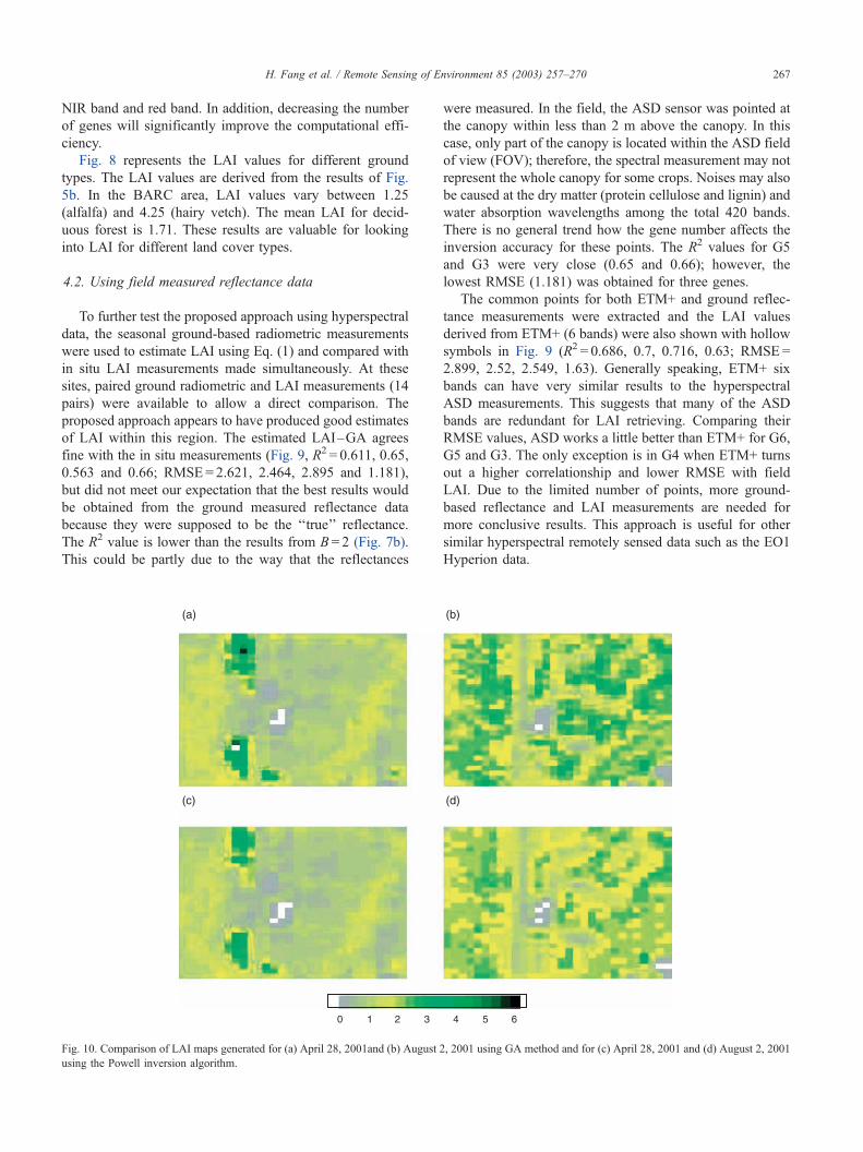
Fig. 10. Comparison of LAI maps generated for (a) April 28, 2001and (b) August 2, 2001 using GA method and for (c) April 28, 2001 and (d) August 2, 2001

using the Powell inversion algorithm.


4.3. Comparison with other methods

It is interesting to compare the GA optimization with

others mentioned in the Introduction. For example, the LUT

method does not have the initial guess selection problem

and the solution is searched over the whole space of canopy

realization. Nonetheless, as pointed out in the Introduction,

the LUT method treats the continuous numerical optimiza-

tion problems as discrete one. In this way, the accuracy of

the database that the LUT needs is based on the coding

accuracy of the input parameters. A comparison of the LUT

method and a neural network approach is provided in

another paper (Fang & Liang, 2003). In that paper, the

GA-based inversion method was compared with the Powell

algorithm in IMCR provided by Kuusk (2001). The Powell

algorithm is often used when there are a large number of

free parameters. It is noted that the GA method used in this

paper does not require the initial guess of the parameters

while the Powell method does. The initial values were

determined based on a priori field knowledge. For compar-

Fig. 11. Comparison of LAI retrieved with GA optimization method (LAI–GA) and with the Powell inversion algorithm (LAI–Powell) for (a) April 28, 2001

and (b) August 2, 2001.

Fig. 12. LAI–NDVI relationships.


ison, an example of the VI approach was also presented at

the end of this section.

The LAI maps (30� 30 pixels) for April 28, 2001 and

August 2, 2001 (Fig. 10) were generated with the same

conditions in Fig. 7b. Their spatial patterns were very

similar although the absolute LAI values may differ. The

brown points were either bare lands or roads, and the gray/

white areas were houses. The yellow and green pixels were

either crops or forests. The estimated LAI–GA values

ranged from 0.12 to 6.02 on April 28, 2001 and from

0.26 to 3.85 on August 2, 2001. However, most LAI on

April 28, 2001 (Fig. 10) is below 4.0. There are only six

dense grass pixels whose LAI–GA is greater than 4.0.

To further examine the similarity and differences be-

tween the two approaches, the LAI data from these two

maps are compared in Fig. 11. Statistical analysis indicated

that there was no significant difference between the LAI

maps generated with the GA optimization method and the

Powell method. LAI–GA tends to be lower than LAI–

Powell, especially when LAI>3. The results of April 28,

2001 (R2 = 0.973) agree better with LAI–Powell than that of

the August 2, 2001 (R2 = 0.864). This maybe due to the low

LAI on April 28, 2001 when 92.1% pixels are less than 2.0

(mean LAI = 1.33). On August 28, 2001, LAI increases

(mean LAI = 2.17) and only 35.8% is less than 2.0.

As mentioned in the Introduction, a large number of

relationships have been established between VIs and LAI

(Baret & Guyot, 1991). The most commonly used vegeta-

tion indices are the simple ratio vegetation index (RVI) and

the normalized difference vegetation index (NDVI). In this

study, it is difficult to use the LAI–VI method as it involves

nine ground covers types on different dates (Table 2). Fig.

12 shows the LAI–NDVI scatterplot with several fitness

curves. NDVI approaches a saturation level for LAI>4.

Generally, both the polynomial and power function fit the

LAI–NDVI poorly. This also necessitates our effort to look

into the GA for retrieving LAI.

5. Summary

In this work, we have explored a new method for

retrieving LAI from Landsat-7 ETM+ images and the field

measured reflectances using the GA optimization methods.

The Markov chain model of canopy reflectance (Kuusk,

2001) was used to simulate the surface reflectance. Both

reflectance data derived from ETM+ image after atmos-

pheric correction and from field measurement were used to

construct the merit function.

Six free parameters, LAI, Sz, Cab, N, rs1 and rs2 (see Table

1), were considered in the retrieval. Different ETM+ band

combinations were tested, i.e., with all six bands, both NIR

and red bands, NIR band and red band. The retrieved LAIwas

in agreement with the measured LAI quite well. Overall, the

best results were obtained with three genes (LAI, rs1 and rs2)

from ETM+ red and NIR bands (R2 = 0.776, RMSE = 1.064).

In general, the result meets the requirement of the Global

Climate Observation System (GCOS) and the Global Terres-

trial Observation System (GTOS) which need an accuracy of

F 0.2–1.0 for terrestrial climate modeling (CEOS/WMO,

2001). The use of six ETM+ bands gets comparable good

results but requires a little more computation. The results

were reasonable when the NIR band was used, but appeared

unacceptable when only the red band was used.

Starting from six, the number of free parameters was

reduced by fixing the least dispersed ones. Four cases were

tested, with six, five, four and three genes by fixing Sz, Cab

and N successively. In this study, reducing the number of

genes does change the inversion accuracy. It can be seen

from Figs. 4–7 that the accuracy of LAI–GA is affected by

the number of genes. As expected, LAI values have large

variations over the study area. The retrieved LAI–GA

values tend to be more stable with fewer genes, which can

be seen from the decreasing standard deviation. Considering

the computational efficiency, we used three genes and both

rad and NIR bands to map the LAI in our study area. The

results using the Powell minimization algorithm were com-

pared with the LAI–GA. The difference between LAI–GA

and LAI–Powell is very small for lower LAI ( < 3) and

increases when LAI>3.

The GA optimization method provides an alternative to

invert the RT models in remote sensing. The advantage of

GA is twofold. First, it scans all the initial conditions and

provides several possible solutions for the detailed exami-

nation of the global optimum solution, thus it avoids the

inaccuracies introduced by traditional minimization algo-

rithms. Second, it only runs the forward RT model with

constrained parameter space and is straightforward in the

optimization process. Experiments are needed to test this

method in more complicated areas. For similar researches, it

is suggested that the minimum number of genes using both

the red and NIR bands be utilized.

In this study, the major computational time was used in

the GA optimization process although reducing the number

of free parameters helps. In the GA, the space of initial

conditions has to be scanned and a large number of

iterations are needed to converge toward appropriate sol-

utions. To solve this problem, more efficient GA optimiza-

tion algorithms and GA-RT coupling methods are needed.

For operational mapping of LAI from the satellite data, the

computational time must be radically reduced before this

method could be extended for regional applications.

Acknowledgements

The work is partially funded by NASA under grants

NAG5-6459 and NCC5462. The authors thank Mingzhen

Chen, Chad Shuey, Andy Russ and Wayne Dulaney for

their contribution to the field campaigns. The authors have

successfully integrated a GA and the MCRM model.

Contact them for details about the integration.


References

Analytical Spectral Devices (ASD) (2000). FieldSpec pro user’s guide.

Baret, F., & Guyot, G. (1991). Potential and limits of vegetation indices

for LAI and APAR assessment. Remote Sensing of Environment, 35,

161–173.

Bicheron, P., & Leroy, M. (1999). A method of biophysical parameter

retrieval at global scale by inversion of a vegetation reflectance model.

Remote Sensing of Environment, 67, 251–266.

CEOS/WMO (Committee for Earth Observation Satellites/World Meteor-

ology Organization), Satellite Systems and Requirements (The Official

CEOS/WMO Online Database), http://alto-stratus.wmo.ch/sat/stations/

SatSystem.html, visited in Dec., 2001.

Chase, T. N., Pielke, R. A., Kittel, T. G. F., S. R., & Nemani, R. (1996).

Sensitivity of a general circulation model to global changes in leaf area

index. Journal of Geophysical Research, 101, 7393–7408.

Clark, C., & Canas, A. (1995). Spectral identification by artificial neural

network and genetic algorithm. International Journal of Remote Sens-

ing, 16(12), 2255–2275.

Davis, L. (1991). Handbook of genetic algorithms. New York: Van

Nostrand-Reinhold.

de Wit, A. J. W. (1999). The Application of a Genetic Algorithm for

Crop Model Steering using NOAA-AVHRR Data, http://cgi.girs.

wageningen-ur.nl/cgi/products/publications.htm.

Fang, H., & Liang, S. (2003). Retrieve LAI from Landsat 7 ETM+ data

with a neural network method: simulation and validation study. IEEE

Transactions on Geoscience and Remote Sensing, (submitted for pub-

lication).

Goel, N. S., & Strebel, D. E. (1983). Inversion of vegetation canopy re-

flectance models for estimating agronomic variables: I. Problem defi-

nition and initial results using the Suits’ model. Remote Sensing of

Environment, 36, 73–104.

Goel, N. S., & Kuusk, A. (1992). Evaluation of one-dimensional analytical

model for vegetation canopies. 12th International Geoscience and Re-

mote Sensing Symposium (IGRASS) ( pp. 505–507).

Goldberg, D. E. (1989). Genetic algorithms in search, optimization and

machine learning. Reading, MA: Addison-Wesley.

Grefenstette, J. (1990). A user’s guide to GENESIS, http://www.aic.nrl.

navy.mil/galist/src/.

Jacquemoud, S. (1993). Inversion of the PROSPECT+SAIL canopy re-

flectance models from AVIRIS equivalent spectra: theoretical study.


Jacquemoud, S., Ustin, S. L., Verdebout, J., Schmuck, G., Andreoli, G., &

Hosgood, B. (1996). Estimating leaf biochemistry using the PROS-

PECT leaf optical properties model. Remote Sensing of Environment,

56, 194–202.

Jin, Y., & Wang, Y. (1999). A genetic algorithm to simultaneously retrieve

land surface roughness and soil wetness. International Journal of Re-

mote Sensing, 22(15), 3093–3099.

Kimes, D. S., Knyazikhin, Y., Privette, J. L., Abuelgasim, A. A., & Gao, F.

(2000). Inversion methods for physically-based models. Remote Sens-

ing Review, 18, 381–440.

Kuusk, A. (1991). The determination of vegetation canopy parameters from

optical measurements. Remote Sensing of Environment, 37, 207–218.

Kuusk, A. (1994). A multispectral canopy reflectance model. Remote Sens-

ing of Environment, 50(2), 75–82.

Kuusk, A. (1995a). A fast invertible canopy reflectance model. Remote

Sensing of Environment, 51, 342–350.

Kuusk, A. (1995b). A Markov chain model of canopy reflectance. Agricul-

tural and Forest Meteorology, 76, 221–236.

Kuusk, A. (2001). A two-layer canopy, reflectance model. Journal of

Quantitative Spectroscopy and Radiative Transfer, 71(1), 1–9.

LAI–COR (1991). LAI–2000 plant canopy analyzer: operating manual

( pp. 4–14).

Liang, S., Fang, H., & Chen, M. (2001). Atmospheric correction of landsat

ETM+ land surface imagery: I. Methods. IEEE Transactions on Geo-

sciences and Remote Sensing, 39(11), 2490–2498.

Liang, S. (2003). Quantitative Remote Sensing of Land Surfaces. New

York: John Wiley and Sons, Inc. (in press).

Liang, S., Fang, H., Morisette, J., Chen, M., Walthall, C., Daughtry, C., &

Shuey, C. (2003). Atmospheric correction of landsat ETM+ land surface

imagery: II. Validation and applications. IEEE Transactions on Geo-

sciences and Remote Sensing (in print).

Liang, S., & Strahler, A. H. (1993). An analytic BRDF model of canopy

radiative transfer and its inversion. IEEE Transaction on Geoscience

and Remote Sensing, 31, 1081–1092.

Liang, S., & Strahler, A. H. (1994). Retrieval of surface BRDF from multi-

angle remotely sensed data. Remote Sensing of Environment, 50, 18–30.

Lin, Y., & Sarabandi, K. (1999). Retrieval of forest parameters using a

fractal-based coherent scattering model and a genetic algorithm. IEEE

Transactions on Geoscience and Remote Sensing, 37(3), 1415–1424.

Myneni, R. B., Maggion, S., Iaquinta, J., Privette, J. L., Gobron, N., Pinty,

B., Kimes, D. S., Verstraete, M. M., & Williams, D. L. (1995). Optical

remote sensing of vegetation: modeling, caveats, and algorithms. Re-

mote Sensing of Environment, 51, 169–188.

Nilson, T., & Kuusk, A. (1989). A reflectance model for the homogeneous

plant canopy and its inversion. Remote Sensing of Environment, 27(2),

157–167.

Pinty, B., Verstraete, M. M., & Dickinson, R. E. (1990). A physical model

for the bidirectional reflectance of vegetation canopies: Part 2. Inversion

and validation. Journal of Geophysical Research, 95, 11767–11775.

Press, W. H., Teukolsky, S. A., Vetterling, W. T., & Plannery, B. P. (1992).

Numerical recipes in C: the art of scientific computing. New York:

Cambridge Univ. Press.

Price, J. C. (1990). On the information content of soil reflectance spectra.


Privette, J. L., Emery, W. J., & Schimel, D. S. (1996). Inversion of a

vegetation reflectance model with NOAA AVHRR data. Remote Sens-

ing of Environment, 58(2), 187–200.

Privette, J. L., Myneni, R. B., Tucker, C. J., & Emery, W. J. (1994).

Invertibility of a 1-D discrete ordinates canopy reflectance model. Re-

mote Sensing of Environment, 48, 89–105.

Rahman, H. (2001). Influence of atmospheric correction on the estimation

of biophysical parameters of crop canopy using satellite remote sensing.

International Journal of Remote Sensing, 22(7), 1245–1268.

Renders, J. M., & Flasse, S. P. (1996). Hybrid methods using genetic

algorithms for global optimization. IEEE Transactions on Systems,

Man, and Cybernetics: Part B. Cybernetics, 26(2), 243–258.

Running, S. W., Nemani, R. R., Peterson, D. L., Band, L. E., Potts, D. F.,

Pierce, L. L., & Spanner, M. A. (1989). Mapping regional forest evapo-

transpiration and photosynthesis by coupling satellite data with ecosys-

tem simulation. Ecology, 70, 1090–1101.

Verhoef, W. (1984). Light scattering by leaf layers with application to

canopy reflectance modeling: the SAIL model. Remote Sensing of En-

vironment, 16, 125–141.

Verstraete, M. M., Pinty, B., & Dickinson, R. E. (1990a). Bidirectional

reflectance of vegetation canopies: Part I. Theory. Journal of Geophys-

ical Research, 95, 11755–11765.

Verstraete, M. M., Pinty, B., & Dickinson, R. E. (1990b). A physical model

of the bidirectional reflectance vegetation canopies: I. Theory. J. Geo-

physical Res., 95(D8), 11755–11765.

Wang, Y., & Jin, Y. (2000). A genetic algorithm to simultaneously retrieve

land surface roughness and soil moisture. Journal of Remote Sensing

(Chinese), 4(2), 90–94.

Weiss, M., & Baret, F. (1999). Evaluation of canopy biophysical variable

retrieval performances from the accumulation of large swath satellite

data. Remote Sensing of Environment, 70, 293–306.

Zhuang, J., & Xu, X. (2000). Genetic algorithms and its application to the

retrieval of component temperature. Remote Sensing for Land and Re-

sources (Chinese), (1), 28–33.


http:\\www.alto-stratus.wmo.ch\sat\stations\SatSystem.html

http:\\www.cgi.girs.wageningen-ur.nl\cgi\products\publications.htm

http:\\www.aic.nrl.navy.mil\galist\src\

retrieving leaf area index using a genetic algorithm with a canopy

Documents