return and volatility spillovers in equity markets: an investigation ...€¦ · return and...

Dedi & Yavas, Cogent Economics & Finance (2016), 4: 1266788http://dx.doi.org/10.1080/23322039.2016.1266788

FINANCIAL ECONOMICS | RESEARCH ARTICLE

Return and volatility spillovers in equity markets: An investigation using various GARCH methodologiesLidija Dedi1* and Burhan F. Yavas2

Abstract: This paper investigates linkages among equity market returns and volatil-ity spillovers in the following countries: Germany, United Kingdom, China, Russia, and Turkey. MARMA, GARCH, GARCH-in-mean, and exponential GARCH (EGARCH) methodologies are applied to daily data on country exchange-traded funds (ETF) based on the MSCI indices from 31 March 2011 to 11 March 2016. The results of the analysis show the existence of significant co-movements of returns among the countries in the sample. ETF returns in Germany, UK, and Russia affect returns in all of the other sample countries. Implications of these findings are explored in terms of portfolio diversification. In addition, the highest volatilities are exhibited by Russia and Turkey. On the other hand, the UK and the Chinese markets have the lowest volatilities. Also, there is a strong evidence of volatility spillovers. All of the countries in the sample, with the exception of UK and Turkey, experience volatility spillovers from other markets. Finally, because of the risk-return trade-off, we analyzed the ef-fect of volatility of the market on its returns and found that only in the UK volatility of the market had a positive effect on its future returns: that an increase in volatility leads to a rise in future ETF returns in the UK.

*Corresponding author: Lidija Dedi, Faculty of Economics & Business, Department of Managerial Economics, University of Zagreb, Zagreb, Croatia E-mails: [email protected], [email protected]

Reviewing editor:David McMillan, University of Stirling, UK

Additional information is available at the end of the article

ABOUT THE AUTHORSLidija Dedi is an associate professor at the University of Zagreb, Faculty of Economics & Business where she teaches undergraduate, graduate, and postgraduate courses in Financial Analysis (Corporate Finance, Investment Analysis, Capital Budgeting, Security Valuation and International Finance). The reported research in this paper is extension of her collaboration with professor Yavas and their research project “International Equity Markets: Performance and valuation.”

Burhan F. Yavas is a professor and department chair (Accounting & Finance) at the California State University-Dominguez Hills where he teaches graduate and undergraduate courses in International Business/Finance. His publications include studies in the areas of international equity markets, international comparative management, intra-industry trade/countertrade, and country risk analysis.

PUBLIC INTEREST STATEMENTThe paper investigates linkages among equity market returns and volatility spillovers in Germany, United Kingdom, China, Russia, and Turkey utilizing MARMA, GARCH, GARCH-in-mean (GARCH-M), and exponential GARCH (EGARCH) methodologies. The results of the analysis show the existence of significant co-movements of returns among the countries in the sample. This finding implies that there are diminishing opportunities for investors to diversify their portfolios. Nevertheless, one could still find significant diversification possibilities for investors. While there is a strong evidence of volatility spillovers markets appear to be more sensitive to the “bad” news than to “good” news. Since volatilities can proxy for risk, there are lessons for both individual and institutional investors in terms of further examining pricing securities, hedging, and other trading strategies as well as framing regulatory policies. The information is also important for policy-makers in the sample countries for understanding the markets’ co-movements and designing policies to avoid unwanted consequences.

Received: 14 October 2016Accepted: 25 November 2016Published: 20 December 2016

of 18

© 2016 The Author(s). This open access article is distributed under a Creative Commons Attribution (CC-BY) 4.0 license.

http://crossmark.crossref.org/dialog/?doi=10.1080/23322039.2016.1266788&domain=pdf&date_stamp=2016-12-20

mailto:[email protected]


http://creativecommons.org/licenses/by/4.0/

of 18


Subjects: Econometrics; International Finance; Investment & Securities

Keywords: ETFs returns; volatility persistence; volatility spillovers; MARMA; GARCH; GARCH-in-mean; EGARCH

JEL codes: G01; G11; G15; C58

1. IntroductionThis paper studies return and volatility linkages among country equity markets using representative broad market index Exchange-Traded Funds or ETFs. The sample consists of the following five coun-tries: Germany, UK, China, Russia, and Turkey. The selection was made mainly with the motivation of studying interactions between equity markets of two stable European countries (Germany and UK) and three of the fastest growing emerging countries of the last decade (China, Russia, and Turkey). The main idea behind the study is if, as the recent research indicates, correlation among equity mar-kets has increased, then unexpected events in one market may affect not only returns but also vola-tilities in other markets. That is, it makes sense to study returns and volatilies together instead of separately.

The pace of global market integration has led to many studies to investigate the mechanism(s) through which equity market movements are transmitted. The main finding has been that while correlations among equity markets have been increasing, there are still opportunities for investors to benefit from portfolio diversifications by investing in different country equity markets (Grosvenor & Greenidge, 2010; Kiymaz, 2003; Kumar, 2013; Yavas & Dedi, 2016; Yavas & Rezayat, 2016). After the 2007–2008 global financial crisis, capital flows across the world responded to policy actions by the major countries. In particular, quantitative easing (QE) by the Federal Reserve Bank (FED), and the Bank of Japan (BOJ) resulted in historicaly low interest rates. However, higher returns (in the form of higher yields in government bonds and interest rates) in some of the emerging markets (e.g. Brazil, Russia, and Turkey) attracted capital flows from the US and the EU; culminating in emerging country equity markets’ spectacular performance until the last quarter of 2013 (Performance.morn-ingstar.com, 2014). While the rates are still close to zero in Europe, US and in Japan the expectation that the FED would soon raise the rates in 2014–2015 gave rise to the reversal of the capital flows since investors started to bring their funds back causing many emerging country currencies to de-preciate. Turkey and Russia, among other emerging markets experienced sizable currency deprecia-tions in the same time frame. The reaction of the equity markets was similar in that many of the equity market indices declined both in terms of local currencies as well as in dollar terms. To defend their currencies both Russia and Turkey raised interest rates. Higher inflation rates (around 9 per-cent) and the need to finance a large current account deficit (around 5% of GDP) even with lower oil prices (Turkey is a net importer of oil), resulted in higher rates in Turkey. Russian rates, on the other hand, have increased due to Western embargo following the Ukrainian conflict and annexation of Crimea together with substantially lower oil prices (Bank, 2015; Stats.oecd.org, 2015).

Consistent with expectations, the FED increased the rates by 25 basis points (0.25) in December 2015 and signaled for more in 2016. However, future rate hikes are not at all certain, given the slug-gish GDP growth in the US and EU as well as in other developed countries like Japan. The Japanese central bank (BOJ) has recently lowered rates to the negative territory. At the same time, the news from the second largest economy in the world (China) have not been encouraging with GDP growth rates consistently hovering below 7%. Recent decision by the British voters to leave the EU has not helped either. It is thus safe to assume that the interest rates will continue to remain low by histori-cal standards.

In addition to near-zero rates in Europe, we have also witnessed depreciation of the Euro from a high of $1.40 per Euro to a low of $1.05 in a period of several months. The depreciation of the Euro (and appreciation of the US dollar) was largely the result of lower yields in Europe and escape from Euro to dollar denominated assets. Note that a short discussion of FED and EU policies is included

of 18


here even though neither US nor EU as a block are included in our study. This is so because the poli-cies of major central banks affect financial flows around the world and by extension they affect eq-uity markets performances.

It should also be noted that equity markets across the world experience growing foreign presence. Investors, heeding the advise of money managers not to put all of their eggs in one basket, have moved part of their portfolios to countries other than their own. The Wall Street Journal reports that about 20% of US nonfinancial shares were held by overseas investors (in 2015) compared to about 10 percent in 2000 (WSJ-March 28, 2016). Similar trends are observed in the UK (54% foreign owner-ship in 2014), in Germany (64%), and Japan (32%). However, increased foreign presence in equity markets globally may be one of the main reasons why they tend to move together in recent years. Generally, stocks, bonds, and property are subject to wild swings in value. When capital moves across borders, these swings are amplified by such things as the lack of knowledge of domestic institutions and exchange-rate risk. Foreign companies that undertake direct investments (buying of factories, building infrastructure) help alleviate lack of domestic savings and investment to speed up GDP growth. However, portfolio investments (buying bonds or stocks) tend to be volatile and the develop-ing countries do not always put inflows of this kind to productive uses and may not able to handle their sudden exit. Some of the short-term foreign borrowing is used to finance long-term domestic loans. The mismatch becomes more pronounced when the borrowing is in foreign currency. If the inflows of “hot money” are sustained, the country may end up having an overvalued currency nega-tively affecting its export businesses. Not surpringly, since the 1996–1997 Asian crisis both econo-mists and politicians started the discussion on capital controls and several (most notably Brazil) implemented entry tax on short-term capital inflows (Ostry, Ghosh, Chamon, & Qureshi, 2011).

The main purpose of this paper is to explore both price and volatility linkages among five selected markets by utilizing broad equity market index-based ETFs. From investors’ perspective, a better understanding of how markets move together may result in superior portfolio construction and hedging strategies, while helping policy-makers (especially central banks) gain an understanding of the processes and consequences of such spillovers. In other words, sheding more light on the infor-mation transmission process among equity markets is important for both micro (asset valuation and risk management) and macro (economic policy and risk management) agents. If market interrela-tions and connectedness are not understood, the results could include implementation of inade-quate or even counterproductive regulatory policies. Therefore, it is important to understand where volatilities arise from, how, and where they are transmitted.

The choice of the data period in this study (31 March 2011–11 March 2016) is especially appropri-ate since it covers a turbulent times with many fiscal and monetary policy decisions in the European Union (and in the US) in the aftermath of 2008 financial crisis with its global effects. The countries in this study were selected for the following reasons: (1) Germany and UK are two important econo-mies representing Europe (EU) and have strong trade and financial ties with Russia and Turkey. (2) Russia and Turkey were among the fastest growing emerging markets which received both direct and portfolio investments from Europe in the 2007–2013 time period. However, both countries suf-fered financial outflows starting with 2014, putting their respective economies at risk. Therefore, the study of equity market interdependencies in such an interesting time period would contribute to the ongoing debate regarding the effect of financial turbulance and its aftermath. In addition, there are not many studies covering equity markets in Russia and Turkey. (3) Finally, China is included in the sample partly because its growing importance in the world but also because many previous studies did not find the Chinese market to be correlated with other equity markets particularly with European markets. We wanted to see if this holds true with recent data and with emerging markets like Russia and Turkey since the latter countries have recently developed significant trade ties with China. In addition, Chinese financial flows (in as well as out) respond to strong US dollar (and the Euro) and affect the value of the Chinese Yuan and by extension the Chinese stock market. In exam-ining the return co-movements, transmission, and persistence of volatilities, we seek to understand if there are opportunities for international investors/traders to earn a better return for a unit of risk.

of 18


The paper uses Exchange-Traded Funds (ETF) instead of benchmark indices. ETFs have lately ex-perienced tremendous growth became the preferred investment vehicles of global investors and hedge funds (Investor.vanguard.com, 2016). Khorana, Nellis, and Trester (1998) and Tse and Martinez (2007) investigate the returns on international ETFs and conclude that ETF returns closely track their respective country indices. Thus, country ETFs and broad based country markets indices are comparable. The advantage of using the ETF data is that one can mitigate, if not entirely avoid, some substantial problems that arise in traditional academic research such as exchange rates vola-tility, divergences in the national tax systems, diversities in stock exchange trading times and bank holidays, restrictions on cross-border trading and investments, and transaction costs.

2. Literature reviewThe central intent behind this paper is to explore price and volatility linkages among the selected coun-try equity markets using ETFs. In doing so, the study contributes to prevalent notable research on country ETFs such as those by Khorana et al. (1998), Tse and Martinez (2007), Hughen and Mathew (2007), and Levy and Lieberman (2013). The present paper differs from the above cited ones in that while they aimed at understanding price dynamics between ETFs and its underlying factors such as NAV, exchange rate, and country indices, we explore price and volatility dynamics amidst country ETFs.

It is clear that, in the context of portfolio allocation/diversification and risk management financial markets deserve in-depth study. Both institutional and individuals make investment decisions that are influenced by perceived higher risk resulting from significant volatilities and their spillovers. The implication is that if equity returns are not highly correlated and there are no significant volatility spillovers then international diversification of investment portfolios would produce benefits since investors can reduce risk without affecting the returns. On the other hand, if equity markets move together and there are significant volatility spillovers then gains from diversification may be small. Portfolio managers would want to have a better handle on the interactions between all equity mar-kets so that they can evaluate market risk and hedging strategies. In addition, economic policy-makers (especially central banks) who are concerned about smooth functioning of financial markets have a keen interest in destabilizing effects of equity market contagion and volatility spillovers. Therefore, a better understanding of the origins and drivers of volatility across markets is important for various market players such as policy-makers, investors, and consumers.

Other studies similar to the present one include Yavas and Dedi (2016) which studies linkages among several European equity markets and Abbas, Khan, and Shah (2013) which investigates the presence of volatility transmission among regional equity markets of Pakistan, China, India, and Sri Lanka in addition to the developed countries (USA, UK, Singapore, and Japan). Their results show that volatility transmission is present between friendly countries of different regions with economic links. They also find some evidence of transmission of volatility between countries, which are on unfriendly terms. Another study by Beirne, Caporale, Schulze-Ghattas, and Spagnolo (2010) exam-ines global (mature) and regional (emerging) spillovers in local emerging stock markets. The results suggest that spillovers from regional and global markets are present in the vast majority of emerg-ing markets. Another finding is that while spillovers in mean returns dominate in emerging Asia and Latin America, spillovers in variance (that is, volatility spillovers) appear to play a key role in emerg-ing markets in Europe. Sakthivel, Bodkhe, and Kamaiah (2012) studies correlation and volatility transmission across stock markets of USA, India, UK, Japan and Australia and found long run co-in-tegration across international stock indices. Additional findings include a bidirectional volatility spillover between US and Indian stock markets and a unidirectional volatility spillover from Japan and United Kingdom to India. Diebold and Yilmaz (2011) provide an empirical analysis of return and volatility spillovers among five equity markets in the Americas: Argentina, Brazil, Chile, Mexico, and the US. Their results indicate that both return and volatility spillovers vary widely. Return spillovers, however, tend to evolve gradually, whereas volatility spillovers display clear bursts that often cor-respond closely to economic events. Li and Giles (2015) examine the linkages of stock markets across the USA, Japan, and six Asian developing countries: China, India, Indonesia, Malaysia, the Philippines, and Thailand. Their results show significant unidirectional shock and volatility spillovers

of 18


from the US market to both the Japanese and the Asian emerging markets. They also find that the volatility spillovers between the US market and the Asian markets are stronger and bidirectional during the Asian financial crisis. Ahmed and Suliman (2011) use symmetric and asymmetric GARCH models to capture volatility clustering and leverage effect at Khartoum Stock Exchange. Their find-ings show that the asymmetric GARCH models may provide better fits than the symmetric models. Oseni and Nwosa (2011) also use EGARCH to examine the volatility in stock market and macroeco-nomic variables utilizing LA-VAR Granger Causality tests applied to Nigeria. Makhwiting, Lesaoana, and Sigauke (2012) used GARCH type models (GARCH, GARCH-M, EGARCH, and TGARCH) for modeling daily returns on the Johannesburg Stock Exchange. Their results show that increased risk does not necessarily imply an increase in returns. Olbryṡ (2013) investigates the asymmetric impact of inno-vations on volatility in the case of the US and three biggest emerging CEEC-3 markets, using univari-ate EGARCH approach. The results indicate that negative innovations have a higher impact on volatility than positive innovations. Baba and Shim (2014) analyses dislocation in the foreign ex-change swap and cross-currency swap markets between Korean and US dollar from 2007 to 2009. Using an EGARCH model, they found that volatility index, the credit default swap spreads of Korean, and US banks are the main factors explaining CIP deviations.

The literature review summarized above has revealed several gaps. First, most of the studies re-viewed above utilize stock market indices as opposed to ETFs used in the present study Second, the present paper uses daily data as opposed to the weekly or monthly data used in other studies. While weekly/monthly data can have advantages in terms of limiting “noise”, daily data provide a larger number of observations. This last point is particularly important because many emerging market ETFs have not been around very long. We also study multi-directional flows, whereas most of the literature focuses on unidirectional flows from the developed to developing markets. Finally, the methodology is somewhat different (vector autoregressive (VAR) as opposed to MARMA) even though the present paper also uses GARCH, GARCH-M, and EGARCH methodologies like most of the other studies. The present paper also addresses the questions of “volatility persistence” in addition to “vol-atility transmission.” The next section describes the data and the methodologies employed. We then present the findings and end the paper with the conclusions and suggestions for future research.

3. Data and basic statisticsThis paper utilizes iShares MSCI Capped/Core Equity ETFs. All Equity ETFs subject to this research are issued by iShares. iShares is the largest ETF provider in the world. Selected ETFs seek to track the in-vestment results of a particular index. For example, The iShares MSCI United Kingdom ETF (EWU) seeks to track the investment results of an index composed of U.K. equities. The data period is from 31 March 2011 to 11 March 2016, a sample of 1,246 days on the following ETFs: (1) The iShares MSCI United Kingdom ETF (EWU); (2) The iShares MSCI Germany ETF (EWG); (3) The iShares MSCI Turkey ETF (TUR); (4) The iShares MSCI Russia Capped ETF (ERUS); (5) The iShares MSCI China ETF (MCHI) (BlackRock, 2016).

As indicated in the introduction, the use of ETFs as opposed to benchmark indices helps mitigate problems such as divergences in the national tax systems, differences in stock exchange trading times and holidays, restrictions on cross-border trading, and exchange rate volatility.

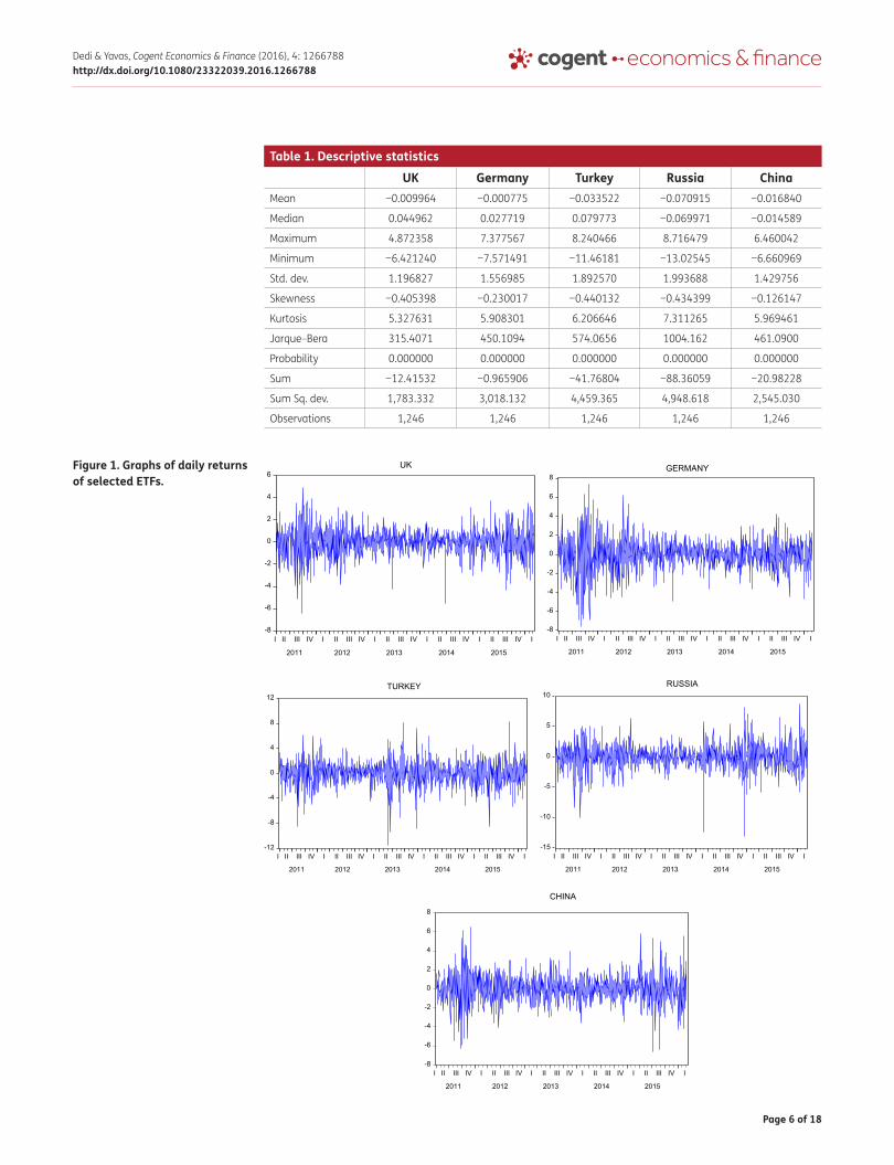
The results from descriptive statistics (Table 1) show that during the period under study, mean ETF returns from all of the countries included in the sample are negative. A visual picture of the return series is shown in Figure 1 indicating clustering of volatility.

Distributional properties of the return series generally appear to be non-normal. Financial markets tend to have “fat tails.” This is so because they are subject to more extreme outcomes in the form of bubbles and crashes. The prime example is nearly 44% fall in 2002, and 40.37% in 2008 in the German’s DAX Index. In addition, markets tend to rise at a slower pace than they fall. After crash in 2008, it took more than five years for the German’s DAX Index to reach the level before crisis (e.g. 8,067.32 on 24 December 2007; 8,042.85 on 11 March 2013) (Value & opportunity, 2014). This gives rise to what is known as “negative skewness” Consistent with these expectations, all five of the

of 18


Table 1. Descriptive statisticsUK Germany Turkey Russia China

Mean −0.009964 −0.000775 −0.033522 −0.070915 −0.016840

Median 0.044962 0.027719 0.079773 −0.069971 −0.014589

Maximum 4.872358 7.377567 8.240466 8.716479 6.460042

Minimum −6.421240 −7.571491 −11.46181 −13.02545 −6.660969

Std. dev. 1.196827 1.556985 1.892570 1.993688 1.429756

Skewness −0.405398 −0.230017 −0.440132 −0.434399 −0.126147

Kurtosis 5.327631 5.908301 6.206646 7.311265 5.969461

Jarque–Bera 315.4071 450.1094 574.0656 1004.162 461.0900

Probability 0.000000 0.000000 0.000000 0.000000 0.000000

Sum −12.41532 −0.965906 −41.76804 −88.36059 −20.98228

Sum Sq. dev. 1,783.332 3,018.132 4,459.365 4,948.618 2,545.030

Observations 1,246 1,246 1,246 1,246 1,246

Figure 1. Graphs of daily returns of selected ETFs.

-8

-6

-4

-2

0

2

4

6

I II III IV I II III IV I II III IV I II III IV I II III IV I

2013 2014 2015

UK

-8

-6

-4

-2

0

2

4

6

8


2013 2014 2015

GERMANY

-12

-8

-4

0

4

8

12


2013 2014 2015

TURKEY

-15

-10

-5

0

5

10


2011 2012 2011 2012

2011 2012 2011 2012 2013 2014 2015

RUSSIA

-8

-6

-4

-2

0

2

4

6

8


2011 2012 2013 2014 2015

CHINA

of 18


countries in sample have negative skewness. The kurtosis or degree of excess, in all markets exceeds three, indicating a leptokurtic distribution. Accordingly, the Jarque–Bera test statistic rejects the null hypothesis of normal distribution for all returns in the sample at α = 0.05 (Table 1).

Looking at the standard deviations, the highest volatility during the period of our study is exhibited by Russia (1.99) followed by Turkey (1.89). The UK market has the lowest volatilitiy (1.19).

4. Methodology

4.1. Multivariate auto regressive moving averages modelTo study co-movements of daily returns, we utilized the Multivariate Auto Regressive Moving Average (MARMA) model which combines some of the characteristics of the univariate autoregressive mov-ing average models and, at the same time, some of the characteristics of regression analysis. They deal with an output time series, yt, which is presumed to be influenced by a vector of input time se-ries Xt, and other inputs collectively grouped and called “noise,” εt. The input series Xt exerts its influ-ence on the output series via a transfer function, which distributes the impact of Xt over several future time periods (Makridakis, Wheelwright, & Hyndman, 1998). The transfer function model, in general, may be represented as:

where φ(L), ω(L), θ(L) are polynomials of different orders in L. Polynomial φ(L) = (1 − φ1 L1 − φ2 L2 − … − φp Lp) represents autoregressive part of order p, “L” denotes lag, L1 yt represents yt−1, and polynomial θ(L) = (1 − θ1 L1 − … − θp Lq) represents moving average part of order q.

4.2. Generalized autoregressive conditional heteroskedasticity modelTo measure the dynamic relationship of the volatility of a process, among the models that can be used are exponential smoothing, autoregressive conditional heteroskedastic (ARCH) and general-ized autoregressive conditional heteroskedastic (GARCH) models. ARCH models were introduced by Engle (1982) and generalized as GARCH by Bollerslev (1986). GARCH models, have become wide-spread tools for dealing with time-series heteroskedasticity and are more widely used to model the conditional volatility of financial series. GARCH models are fitted when errors of AR or ARMA or in general a regression model have variances which are not independent or the variance in the current error term is related to the value of the previous periods’ error terms as well as past variances. The coefficients of the past periods’ squared error terms are indicative of the strength of the shocks in the short term, while the coefficient of the past variances (GARCH effect) measures the contribution of these shocks to long-run persistence (Grosvenor & Greenidge, 2010).

The specification of a typical GARCH model is given by:

and �2t|ψt−1~N(0, �2

t−1) is the innovation in the asset return and ψt−1 = {yt−1,εt−1, yt−2, εt−2 …), where yt−i,

represent the return at time t−i and ɛi is the error resulted of a regression or an ARMA model fitted to returns. Similar to ARMA models where β (L) of order p is the autoregressive term and polynomial α (L) of order q is the moving average term.

GARCH processes have commonly tails heavier than the normal distribution. This property makes the GARCH process attractive because the distribution of asset returns frequently display tails heavier than the normal distribution. In most empirical applications with finitely sampled data, the simple ARCH (1) or GARCH (1, 1) is found to provide a fair description of the data. ARCH (1) model is as follows:

(1)�(L)Yt= �(L)X

t+ �(L)�

t

(2)�2

t= � + �(L)�2t−1 + �(L)�2t

(3)�2

t= � + ��

2

t−1

of 18


A sufficient condition for the conditional variance to be positive is that the parameters of the model satisfy the following constraints: ω > 0 and α > 0.

GARCH (1, 1) model is:

α is the coefficient that measures the extent to which a volatility shock today feeds through the next period volatility, while α + β is usually considered to be a measure of persistence of volatility shock and it measures the rate at which this effect dies over time.

Note that when yt, the rate of return on an asset is not function of a regressors (that there is no regression component in the model), then yt is identical to et and becomes a pure GARCH process. In this study, we use GARCH (1, 1) to analyze the persistence of conditional volatility of the returns as well as transmission of volatility of returns. Daily ETF returns are calculated by 100* logarithmic dif-ference of daily closing ETF values. rt = 100 * d log (pt).

4.3. GARCH-in-meanEngle, Lilien, and Robins (1987) suggested an ARCH in mean model (ARCH-M), where the conditional variance of asset returns enters into the conditional mean equation. Bollerslev, Engle, and Wooldridge (1988) extend the ARCH-M model to the GARCH-M (GARCH-in-mean). GARCH-M is an extension of GARCH model, which takes into account risk-return trade off. This is important since investors expect higher rates of return for riskier investments. GARCH-M model is given by specification (Brooks, 2014, p. 445)

If δ is positive and statistically significant, then increased risk, given by an increase in the conditional variance, leads to a rise in the mean return. Thus, δ can be interpreted as a risk premium (Brooks, 2014, p. 445).

4.4. EGARCHIt has been shown that the symmetric GARCH models may not capture some important features of the data since they assume a symmetric response of volatility to positive and negative shocks (Brooks, 2014). Therefore, different types of GARCH models that modify the conditional variance Equation (4) have been proposed. Among them, three GARCH models that allow volatility to respond asymmetrically to both positive and negative returns have received wide acceptance: AGARCH, TGARCH (GRJ), and EGARCH (Alexander, 2008; Brooks, 2014). Both AGARCH and TGRACH simply mod-ify the symmetric GARCH equation to capture asymmetric effects. In TGARCH (GRJ), which is an al-ternative formulation to AGARCH, asymmetric response is rewritten to specifically augment the volatility response from only the negative market shocks. Also, it is not always easy to optimize a TGARCH (GJR) model. Consequently, we used EGARCH model (Nelson, 1991), as recommended by Alexander (2008). The EGARCH is an asymmetric model that specifies the logarithm of the condi-tional volatility and avoids the need for any parameters constraints.

Nelson (1991) proposed exponential GARCH or EGARCH model to capture asymmetric effect.

(4)𝜎2

t= 𝜔 + 𝛼𝜀

2

t−1+ 𝛽𝜎

2

t−1𝜔 > 0, 0 < 𝛽 ≤ 1, 0 < 𝛼 ≤ 1, 𝛼 + 𝛽 ≤ 1

(5)yt= � + ��

t−1+ u

t, u

t∼ N

(0,�2

t

)

(6)�2

t= �

0+ �

1u2t−1

+ ��2

t−1

(7)ln��2

t

�= � + � ln

��2

t−1

�+ �

�t−1��2

t−1

+ �

⎡⎢⎢⎢⎣

��t−1��2

t−1

−√2∕�

⎤⎥⎥⎥⎦

of 18


where �, �, � and � are constant parameters. The EGARCH model is asymmetric because the level

of �t−1

∕

√�2

t−1 is included with a coefficient γ. Since this asymmetry coefficient γ is typically nega-

tive, positive return shocks generate less volatility then negative return shocks, all else equal. The EGARCH model differs from the standard GARCH model in two main respects (Engle & Ng, 1993, pp. 1752, 1753):

(1) The EGARCH model allows good news and bad news to have a different impact on volatility, while the standard GARCH model does not, and

(2) The EGARCH model allows big news to have a greater impact on volatility than the standard GARCH model.

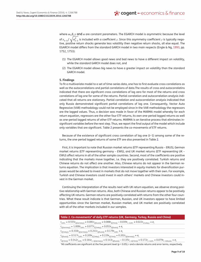
5. FindingsTo fit a multivariate model to a set of time-series data, one has to first evaluate cross correlations as well as the autocorrelations and partial correlations of data.The results of cross and autocorrelatins indicated that there are significant cross correlations of lag zero for most of the returns and cross correlations of lag one for some of the returns. Partial correlation and autocorrelation analysis indi-cated that all returns are stationary. Partial correlation and autocorrelation analysis indicated that only Russia demonstrated significant partial correlations of lag one. Consequently, Vector Auto Regressive (VAR) methodology could not be employed since in the VAR methodology the regressors are the lagged values. Thus, a decision was made in favor of the MARMA model whereby for each return equation, regressors are the other four ETF returns, its own one-period lagged returns as well as one-period lagged returns of other ETF returns. MARMA is an iterative process that eliminates in-significant variables before the next step. Thus, we report the final output of the model which include only variables that are significant. Table 2 presents the co-movements of ETF returns.

Because of the existence of significant cross correlation of lag one (t−1) among some of the re-turns, the one-period lagged returns of some ETF are also presented in Table 2.

First, it is important to note that Russian market returns (ETF representing Russia – ERUS), German market returns (ETF representing germany – EWG), and UK market returns (ETF representing UK – EWU) affect returns in all of the other sample countries. Second, most of the coefficients are positive indicating that the markets move together, i.e. they are positively correlated. Turkish returns and Chinese returns do not affect one another. Also, Chinese returns do not appear in the German re-turns equation. The implication is that investors interested in equity markets for diversification pur-poses would be advised to invest in markets that do not move together with their own. For example, Turkish and Chinese investors could invest in each others’ markets and Chinese investors could in-vest in the German market.

Continuing the interpretation of the results next with UK return equation, we observe strong posi-tive relationship with German returns. Also, both Chinese and Russian returns appear to be positively affecting UK returns. German returns are positively correlated with returns from the other four coun-tries. What these result indicate is that German, Russian, and UK investors appear to have limited opportunities since the German market, Russian market, and UK market are positively correlated with all of the other markets included in our samples.

Table 2. Co-movements* of daily ETF returns (UK, Germany, Turkey, Russia and China)

*All coefficients are significant at the five percent level (p < 0.05); r and e denote returns and error terms, respectively.

rt(UK) = 0.555rt(Germany) + 0.081rt(Russia) + 0.088rt(China) − 0.039rt−1(UK) + 0.023rt(Turkey) + et

rt(Germany) = 1.000rt(UK) + 0.077rt(Turkey) + 0.053rt(Russia) + et

rt(Turkey) = 0.310rt(Germany) + 0.241rt(Russia) + 0.179rt(UK) + et

rt(Russia) = 0.517rt(UK) + 0.209rt(Turkey) + 0.229rt(China) + 0.202rt(Germany) + et

rt(China) = 0.342rt(UK) + 0.164rt−1(Germany) + 0.143rt(Russia) − 0.135rt−1(China) + 0.172rt−1(UK) + 0.079rt−1(Russia) + et

of 18


The above results are in line with what other recent research has found. For example, several stud-ies have all indicated that financial contagion has increased in Latin America (Kiymaz, 2003), in Europe (Gray, 2009), and in emerging markets of BRIC and MIST (Yavas & Rezayat, 2016).

In order to study the volatility and its persistency or transmission using a GARCH-type model it is a common practice to compute Engle (1982) test for ARCH effects to make sure that this class of models is appropriate for the data. The Engle test results for sample countries confirmed the pres-ence of ARCH in the ETFs returns indicating the appropriateness of the model.

5.1. Volatility persistenceVolatility persistence deals with the nature of volatility and whether the current period’s volatility is affected by past periods’ volatility.

To analyze persistence in volatility, GARCH (1, 1) specification is commonly used. The literature referred to above indicates that the sum of the ARCH and GARCH effects is a measure of volatility persistence. If that sum is closer to one, it means that effects of shocks fade away very slowly. The lower the values of GARCH & ARCH effects, the faster the effects fade away.

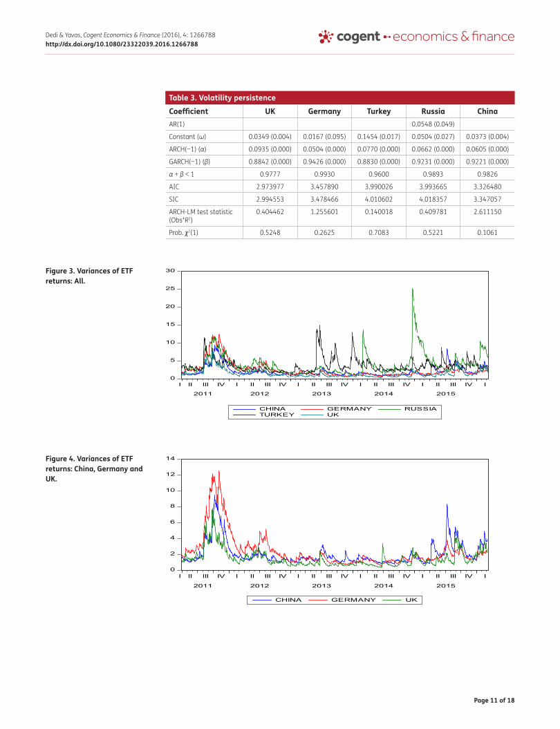
Arch reaction parameter, α usually ranges between 0.05 (for a market that is relatively stable) and about 0.1 (for a market that is jumpy). In other words, α measures the extent to which shocks to today’s returns feed through into volatility of next period, and α + β measures the rate in which this effect dies over time. Table 3 presents volatility persistence for selected countries.

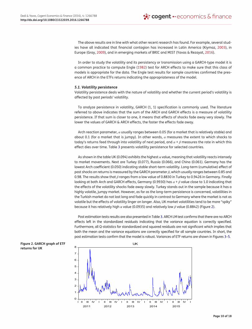
As shown in the table UK (0.094) exhibits the highest α value, meaning that volatility reacts intensely to market movements. Next are Turkey (0.077), Russia (0.066), and China (0.061). Germany has the lowest Arch coefficient (0.050) indicating stable short-term volatility. Long-term (cumulative) effect of past shocks on returns is measured by the GARCH parameter β, which usually ranges between 0.85 and 0.98. The results show that β ranges from a low value of 0.8830 in Turkey to 0.9426 in Germany. Finally looking at both Arch and GARCH effects, Germany (0.9930) has α + β value close to 1.0 indicating that the effects of the volatility shocks fade away slowly. Turkey stands out in the sample because it has a highly volatile, jumpy market. However, as far as the long-term persistence is concerned, volatilities in the Turkish market do not last long and fade quickly in contrast to Germany where the market is not as volatile but the effects of volatility linger on longer. Also, UK market volatilities tend to be more “spiky” because it has relatively high α value (0.0935) and relatively low β value (0.8842) (Figure 2).

Post estimation tests results are also presented in Table 3. ARCH LM test confirms that there are no ARCH effects left in the standardized residuals indicating that the variance equation is correctly specified. Furthermore, all Q-statistics for standardized and squared residuals are not significant which implies that both the mean and the variance equations are correctly specified for all sample countries. In short, the post estimation tests confirm that the model is robust. Variances of ETF returns are shown in Figures 3–5.

Figure 2. GARCH graph of ETF returns for UK

0

1

2

3

4

5

6

7

8


2011 2012 2013 2014 2015

UK

of 18


Figure 4. Variances of ETF returns: China, Germany and UK.

0

2

4

6

8

10

12

14


2011 2012 2013 2014 2015

CHINA GERMANY UK

Figure 3. Variances of ETF returns: All.

0

5

10

15

20

25

30


2011 2012 2013 2014 2015

CHINA GERMANY RUSSIATURKEY UK

Table 3. Volatility persistenceCoefficient UK Germany Turkey Russia ChinaAR(1) 0.0548 (0.049)

Constant (ω) 0.0349 (0.004) 0.0167 (0.095) 0.1454 (0.017) 0.0504 (0.027) 0.0373 (0.004)

ARCH(−1) (α) 0.0935 (0.000) 0.0504 (0.000) 0.0770 (0.000) 0.0662 (0.000) 0.0605 (0.000)

GARCH(−1) (β) 0.8842 (0.000) 0.9426 (0.000) 0.8830 (0.000) 0.9231 (0.000) 0.9221 (0.000)

α + β < 1 0.9777 0.9930 0.9600 0.9893 0.9826

AIC 2.973977 3.457890 3.990026 3.993665 3.326480

SIC 2.994553 3.478466 4.010602 4.018357 3.347057

ARCH-LM test statistic (Obs*R2)

0.404462 1.255601 0.140018 0.409781 2.611150

Prob. χ2(1) 0.5248 0.2625 0.7083 0.5221 0.1061

of 18


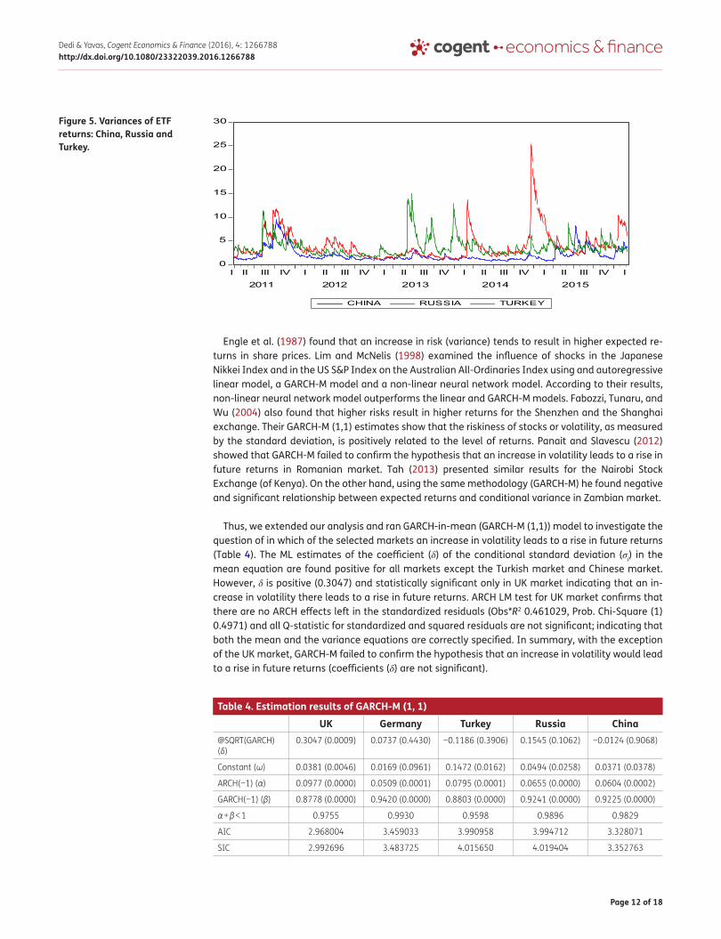
Engle et al. (1987) found that an increase in risk (variance) tends to result in higher expected re-turns in share prices. Lim and McNelis (1998) examined the influence of shocks in the Japanese Nikkei Index and in the US S&P Index on the Australian All-Ordinaries Index using and autoregressive linear model, a GARCH-M model and a non-linear neural network model. According to their results, non-linear neural network model outperforms the linear and GARCH-M models. Fabozzi, Tunaru, and Wu (2004) also found that higher risks result in higher returns for the Shenzhen and the Shanghai exchange. Their GARCH-M (1,1) estimates show that the riskiness of stocks or volatility, as measured by the standard deviation, is positively related to the level of returns. Panait and Slavescu (2012) showed that GARCH-M failed to confirm the hypothesis that an increase in volatility leads to a rise in future returns in Romanian market. Tah (2013) presented similar results for the Nairobi Stock Exchange (of Kenya). On the other hand, using the same methodology (GARCH-M) he found negative and significant relationship between expected returns and conditional variance in Zambian market.

Thus, we extended our analysis and ran GARCH-in-mean (GARCH-M (1,1)) model to investigate the question of in which of the selected markets an increase in volatility leads to a rise in future returns (Table 4). The ML estimates of the coefficient (δ) of the conditional standard deviation (σi) in the mean equation are found positive for all markets except the Turkish market and Chinese market. However, δ is positive (0.3047) and statistically significant only in UK market indicating that an in-crease in volatility there leads to a rise in future returns. ARCH LM test for UK market confirms that there are no ARCH effects left in the standardized residuals (Obs*R2 0.461029, Prob. Chi-Square (1) 0.4971) and all Q-statistic for standardized and squared residuals are not significant; indicating that both the mean and the variance equations are correctly specified. In summary, with the exception of the UK market, GARCH-M failed to confirm the hypothesis that an increase in volatility would lead to a rise in future returns (coefficients (δ) are not significant).

Table 4. Estimation results of GARCH-M (1, 1)UK Germany Turkey Russia China

@SQRT(GARCH) (δ)

0.3047 (0.0009) 0.0737 (0.4430) −0.1186 (0.3906) 0.1545 (0.1062) −0.0124 (0.9068)

Constant (ω) 0.0381 (0.0046) 0.0169 (0.0961) 0.1472 (0.0162) 0.0494 (0.0258) 0.0371 (0.0378)

ARCH(−1) (α) 0.0977 (0.0000) 0.0509 (0.0001) 0.0795 (0.0001) 0.0655 (0.0000) 0.0604 (0.0002)

GARCH(−1) (β) 0.8778 (0.0000) 0.9420 (0.0000) 0.8803 (0.0000) 0.9241 (0.0000) 0.9225 (0.0000)

α + β < 1 0.9755 0.9930 0.9598 0.9896 0.9829

AIC 2.968004 3.459033 3.990958 3.994712 3.328071

SIC 2.992696 3.483725 4.015650 4.019404 3.352763

Figure 5. Variances of ETF returns: China, Russia and Turkey.

0

5

10

15

20

25

30


2011 2012 2013 2014 2015

CHINA RUSSIA TURKEY

of 18


To assess the robustness of the GARCH (1, 1) and GARCH-M (1, 1) models for UK market we com-pared AIC and SIC criterion. For GARCH-in-mean (1, 1) AIC criterion is slightly lower for UK market than for GARCH (1, 1) (2.968004 < 2.973977). On the other hand, SIC criterion is almost the same for both models (GARCH-in-mean SIC 2.992696; GARCH (1, 1) SIC 2.994553). For the UK market the GARCH-in-mean (1, 1) is slightly better model than the GARCH (1, 1).

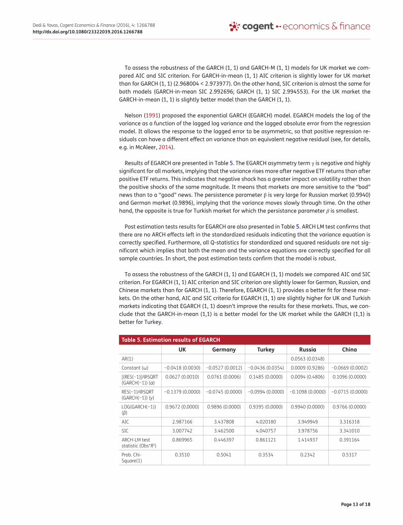
Nelson (1991) proposed the exponential GARCH (EGARCH) model. EGARCH models the log of the variance as a function of the lagged log variance and the lagged absolute error from the regression model. It allows the response to the lagged error to be asymmetric, so that positive regression re-siduals can have a different effect on variance than an equivalent negative residual (see, for details, e.g. in McAleer, 2014).

Results of EGARCH are presented in Table 5. The EGARCH asymmetry term γ is negative and highly significant for all markets, implying that the variance rises more after negative ETF returns than after positive ETF returns. This indicates that negative shock has a greater impact on volatility rather than the positive shocks of the same magnitude. It means that markets are more sensitive to the “bad” news than to a “good” news. The persistence parameter β is very large for Russian market (0.9940) and German market (0.9896), implying that the variance moves slowly through time. On the other hand, the opposite is true for Turkish market for which the persistance parameter β is smallest.

Post estimation tests results for EGARCH are also presented in Table 5. ARCH LM test confirms that there are no ARCH effects left in the standardized residuals indicating that the variance equation is correctly specified. Furthermore, all Q-statistics for standardized and squared residuals are not sig-nificant which implies that both the mean and the variance equations are correctly specified for all sample countries. In short, the post estimation tests confirm that the model is robust.

To assess the robustness of the GARCH (1, 1) and EGARCH (1, 1) models we compared AIC and SIC criterion. For EGARCH (1, 1) AIC criterion and SIC criterion are slightly lower for German, Russian, and Chinese markets than for GARCH (1, 1). Therefore, EGARCH (1, 1) provides a better fit for these mar-kets. On the other hand, AIC and SIC criteria for EGARCH (1, 1) are slightly higher for UK and Turkish markets indicating that EGARCH (1, 1) doesn’t improve the results for these markets. Thus, we con-clude that the GARCH-in-mean (1,1) is a better model for the UK market while the GARCH (1,1) is better for Turkey.

Table 5. Estimation results of EGARCHUK Germany Turkey Russia China

AR(1) 0.0563 (0.0348)

Constant (ω) −0.0418 (0.0030) −0.0527 (0.0012) −0.0436 (0.0354) 0.0009 (0.9286) −0.0669 (0.0002)

|(RES(−1)|/@SQRT (GARCH(−1)) (α)

0.0627 (0.0010) 0.0761 (0.0006) 0.1485 (0.0000) 0.0094 (0.4806) 0.1096 (0.0000)

RES(−1)/@SQRT (GARCH(−1)) (γ)

−0.1379 (0.0000) −0.0745 (0.0000) −0.0994 (0.0000) −0.1098 (0.0000) −0.0715 (0.0000)

LOG(GARCH(−1)) (β)

0.9672 (0.0000) 0.9896 (0.0000) 0.9395 (0.0000) 0.9940 (0.0000) 0.9766 (0.0000)

AIC 2.987166 3.437808 4.020180 3.949949 3.316318

SIC 3.007742 3.462500 4.040757 3.978756 3.341010

ARCH-LM test statistic (Obs*R2)

0.869965 0.446397 0.861121 1.414937 0.391164

Prob. Chi-Square(1)

0.3510 0.5041 0.3534 0.2342 0.5317

of 18


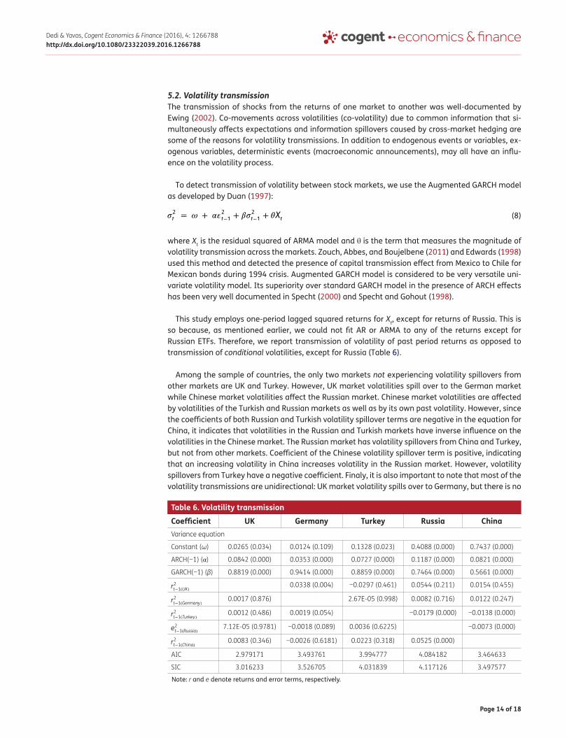
5.2. Volatility transmissionThe transmission of shocks from the returns of one market to another was well-documented by Ewing (2002). Co-movements across volatilities (co-volatility) due to common information that si-multaneously affects expectations and information spillovers caused by cross-market hedging are some of the reasons for volatility transmissions. In addition to endogenous events or variables, ex-ogenous variables, deterministic events (macroeconomic announcements), may all have an influ-ence on the volatility process.

To detect transmission of volatility between stock markets, we use the Augmented GARCH model as developed by Duan (1997):

where Xt is the residual squared of ARMA model and θ is the term that measures the magnitude of volatility transmission across the markets. Zouch, Abbes, and Boujelbene (2011) and Edwards (1998) used this method and detected the presence of capital transmission effect from Mexico to Chile for Mexican bonds during 1994 crisis. Augmented GARCH model is considered to be very versatile uni-variate volatility model. Its superiority over standard GARCH model in the presence of ARCH effects has been very well documented in Specht (2000) and Specht and Gohout (1998).

This study employs one-period lagged squared returns for Xt, except for returns of Russia. This is so because, as mentioned earlier, we could not fit AR or ARMA to any of the returns except for Russian ETFs. Therefore, we report transmission of volatility of past period returns as opposed to transmission of conditional volatilities, except for Russia (Table 6).

Among the sample of countries, the only two markets not experiencing volatility spillovers from other markets are UK and Turkey. However, UK market volatilities spill over to the German market while Chinese market volatilities affect the Russian market. Chinese market volatilities are affected by volatilities of the Turkish and Russian markets as well as by its own past volatility. However, since the coefficients of both Russian and Turkish volatility spillover terms are negative in the equation for China, it indicates that volatilities in the Russian and Turkish markets have inverse influence on the volatilities in the Chinese market. The Russian market has volatility spillovers from China and Turkey, but not from other markets. Coefficient of the Chinese volatility spillover term is positive, indicating that an increasing volatility in China increases volatility in the Russian market. However, volatility spillovers from Turkey have a negative coefficient. Finaly, it is also important to note that most of the volatility transmissions are unidirectional: UK market volatility spills over to Germany, but there is no

(8)�2

t= � + ��

2

t−1+ ��

2

t−1+ �X

t

Table 6. Volatility transmission

Note: r and e denote returns and error terms, respectively.

Coefficient UK Germany Turkey Russia ChinaVariance equation

Constant (ω) 0.0265 (0.034) 0.0124 (0.109) 0.1328 (0.023) 0.4088 (0.000) 0.7437 (0.000)

ARCH(−1) (α) 0.0842 (0.000) 0.0353 (0.000) 0.0727 (0.000) 0.1187 (0.000) 0.0821 (0.000)

GARCH(−1) (β) 0.8819 (0.000) 0.9414 (0.000) 0.8859 (0.000) 0.7464 (0.000) 0.5661 (0.000)

r2t−1(UK) 0.0338 (0.004) −0.0297 (0.461) 0.0544 (0.211) 0.0154 (0.455)

r2t−1(Germany) 0.0017 (0.876) 2.67E-05 (0.998) 0.0082 (0.716) 0.0122 (0.247)

r2t−1(Turkey) 0.0012 (0.486) 0.0019 (0.054) −0.0179 (0.000) −0.0138 (0.000)

e2t−1(Russia) 7.12E-05 (0.9781) −0.0018 (0.089) 0.0036 (0.6225) −0.0073 (0.000)

r2t−1(China) 0.0083 (0.346) −0.0026 (0.6181) 0.0223 (0.318) 0.0525 (0.000)

AIC 2.979171 3.493761 3.994777 4.084182 3.464633

SIC 3.016233 3.526705 4.031839 4.117126 3.497577

of 18


transmission from Germany to UK. Similarly, Turkish market volatilities are transmitted to China but there is no corresponding flow to Turkey. In general, therefore, the findings do not point to a very close integration among the markets studied in that financial turmoil in some markets does not trig-ger headwinds for other markets. This is in contrast to findings from studies that include major European markets (Yavas & Dedi, 2016). Therefore, financial contagion is far from reality when it comes to such different markets as the ones included in this study with the exception of the UK and the German markets that appear to be closely integrated. The above results have implications for investors as well as policy-makers. For the European money managers/investors in UK and in Germany, emerging equity markets like China, Russia, and Turkey represent excellent vehicles of portfolio diversification even though investing in each others’ markets would not reduce their port-folio risk. Chinese, Russian, and Turkish investors could also lower their risk by investing in other markets included in the sample.

As alluded to in the introduction, understanding the transmission process between markets is critical for risk management and economic policy. A lack of such understanding could result in inad-equate or even counterproductive regulatory policies. For example, the findings of significant volatil-ity transmission between the UK and the German markets may provide impetus for the push for greater co-operation between the policy-makers in both countries even though such a prospect is not likely especially after the Brexit vote in June 2016. In general, evidence of volatility spillovers (or lack thereof) would offer an understanding on the degree of openness and economic co-depend-ence of economies. Many emerging countries have implemented policies of financial liberalization which in turn resulted in increased capital inflows—both portfolio and the direct investment type. Short-term portfolio investments by portfolio managers and hedge funds have brought about con-cerns regarding their stability and calls for their regulation (Ostry et al., 2011).

On the other hand, there is also a risk of financial crisis originating from emerging markets and the risk of exposure to these economies. The case in point may be the drop in commodity prices in after the 2007–2008 financial crisis and their effect on commodity exporters such as Russia and Brazil. Clearly, central bankers and other financial policy-makers would benefit from this line of research and may become better equipped to cope with contagion effects of shocks among markets.

In summary, it may be concluded that during the period covering this study (2011–2016), there is some evidence of cross-transmission of volatility between the stock markets. These results are cor-roborated by Beirne et al. (2010) and Yavas and Dedi (2016) that find spillovers in variance (volatility) appear to play a role in Europe. Schleicher (2001), on the other hand, found return co-movements significant but not their volatilities in Hungary, Poland, and Czech Republic.

6. ConclusionsThis paper studied the transmission of equity returns and volatility. A Multivariate Autoregressive Moving Average (MARMA) model along with univariate Generalized Autoregressive Conditional Heteroscedastic (GARCH) models are used (including both symmetric and asymmetric models) to capture most common stylized facts about ETF returns.

The key findings are: co-movements between daily ETF returns representing the countries under study are significant. This finding implies that there are diminishing opportunities for investors to diversify their portfolios. Nevertheless, one could still find significant diversification possibilities for investors. For example, Chinese and Turkish investors can safely diversify by investing in each other’s markets. German, Russian, and UK investors, on the other hand, appear to have limited opportunities since the German market, UK market, and Russian market are positively correlated with all of the other markets included in our samples.

Another finding of the study indicates that among the sample countries, Russia and Turkey are more volatile than the developed markets (UK and Germany). Once again, these results are similar

of 18


to findings of other studies (Abbas et al., 2013; Beirne et al., 2010; Frankel & Roubini, 2001; Yavas & Rezayat, 2016).

Clearly, higher market returns are desired by investors, but higher returns always accompany higher risk. In fact, higher returns compensate for the excess risk of the investment. Market volatility measures the uncertainty of returns and the riskiness of various equity markets. Changing volatility in other (international) markets may also affect volatility in the domestic equity market. Therefore, regulatory authorities would like to evaluate the impacts of volatility spillovers. This is so because when shocks happen in closely linked markets, the effectiveness of monetary policies may be limit-ed. Equity market interdependence while lowering potential gain from global diversification provides a transmission channel for volatility shocks.

We also found evidence of volatility spillovers. The results show that the only two markets not experiencing volatility spillovers from other markets are UK and Turkey. On the other hand, Russian market has volatility spillovers from China and Turkey, but not from other markets. German market is affected only by volatility in UK. Most of the volatility transmissions are unidirectional: UK market volatility spills over to Germany, but there is no transmission from Germany to UK. Similarly, Turkish market volatilities are transmitted to China but there is no corresponding flow to Turkey.

The results of the GARCH-in-mean (GARCH-M (1, 1)) model indicated that an increase in volatility leads to a rise in future returns only in the context of the UK market. That is, the GARCH-M model failed to confirm the hypothesis that an increase in volatility leads to a rise in future returns in the markets other than the UK.

Finally, the results of the EGARCH (1, 1) model indicated that markets are more sensitive to the “bad” news than to a “good” news. However, the overall analysis indicates that EGARCH (1, 1) is bet-ter model only for German, Russian, and Chinese markets, indicating that positive return shocks generate less volatility then negative return shocks. On the other hand, GARCH-M is better for the UK market and GARCH (1, 1) for Turkish market.

Since volatilities can proxy for risk, there are lessons for both individual and institutional investors in terms of further examining pricing securities, hedging, and other trading strategies as well as framing regulatory policies. The information is also important for policy-makers in the sample coun-tries for understanding the markets’ co-movements and designing policies.

Consider as an example a recently constructed product as a hedge against a risk of market melt-down. The product is an exchange-traded fund based on VIX, a measure of market volatility. The ETF invests in VIX futures contracts. It shifts from long-erm to short-term contracts (and vice versa) when the VIX moving average reaches a certain threshold. The main idea behind this strategy is to allow investors to benefit from sudden spikes in volatility while keeping the ETFs overall costs down (Economist, Febuary 25–March 2, 2012). Equity market volatility can be used by investors in such a strategy. It is clear that innovation in both ETFs and their volatilities continue. Because of the rela-tionship between volatilities and risks, volatility transmissions open up a new area for financial prod-ucts that are tailor-made to allow investors to benefit from (or hedge against) sudden changes in market volatility.

Although we argued in favor of using ETFs as a vehicle for diversification a warning may be ap-propriate: During the flash crash of 2010 in the USA when the Dow Jones industrial average dropped almost 1,000 points, the heavy losses in the futures markets quickly spilled over into the ETF market resulting in many investors shorting the ETF that tracked the underlying indexes. This link may indi-cate again that some of the newer financial products such as ETFs have not been around long enough to be tested for crisis situations.

of 18


Another interesting extension would be to split the data into two parts mirroring periods of rapid run-up in dollar denominated emerging market debt (lower rates in US and EU) and the subsequent sharp slowdown in GDP due to drying up of liquidity. The final recommendation includes the expan-sion of the investigation to other countries in both in Europe and in Asia to study spillovers.

FundingThe authors received no direct funding for this research.

Author detailsLidija Dedi1

E-mails: [email protected], [email protected] ID: http://orcid.org/0000-0003-2964-198XBurhan F. Yavas2

E-mail: [email protected] Faculty of Economics & Business, Department of Managerial

Economics, University of Zagreb, Zagreb, Croatia.2 Department of Accounting, Finance & Economics, California

State University-Dominguez Hills, Carson, CA 90747, USA.

Citation informationCite this article as: Return and volatility spillovers in equity markets: An investigation using various GARCH methodologies, Lidija Dedi & Burhan F. Yavas, Cogent Economics & Finance (2016), 4: 1266788.

ReferencesAbbas, Q., Khan, S,, & Shah, Z. (2013). Volatility transmission in

regional Asian stock markets. Emerging Markets Review, 16, 66–77. doi:10.1016/j.ememar.2013.04.004

Ahmed, A. E. M., Suliman, S. Z. (2011). Modeling stock market volatility using GARCH models evidence from Sudan. International Journal of Business and Social Science, 2, 114–128.

Alexander, C. (2008). Practical financial econometrics, market risk analysis (Vol. II). West Sussex: Wiley.

Baba, N., & Shim, I. (2014). Dislocations in the won-dollar swap markets during the crisis of 2007–2009. International Journal of Finance & Economics, 19, 279–302. doi:10.1002/ijfe.1492

Beirne, J., Caporale, G., Schulze-Ghattas, M., & Spagnolo, N. (2010). Global and regional spillovers in emerging stock markets: A multivariate GARCH-in-mean analysis. Emerging Markets Review, 11, 250–260. doi:10.1016/j.ememar.2010.05.002

Bollerslev, T. (1986). Generalized autoregressive conditional heteroskedasticity. Journal of Econometrics, 31, 307–327. http://dx.doi.org/10.1016/0304-4076(86)90063-1

Bollerslev, T., Engle, R. F., & Wooldridge, J. M. (1988). A capital asset pricing model with time-varying covariances. Journal of Political Economy, 96, 116–131. http://dx.doi.org/10.1086/261527

Brooks, C. (2014). Introductory econometrics for finance (3rd ed.). Cambridge: Cambridge University Press.

Diebold, F. X., & Yilmaz, K. (2011). Equity market spillovers in the Americas. In R. Alfaro (ed.) Financial stability, monetary policy, and central banking (Vol. 15, pp. 199–214). Santiago: Bank of Chile Central Banking Series.

Duan, J. C. (1997). Augmented GARCH (p, q) process and its diffusion limit. Journal of Econometrics, 79, 97–127. http://dx.doi.org/10.1016/S0304-4076(97)00009-2

Edwards, S. (1998). Interest rate volatility, capital controls, and contagion (NBER Working Paper Series). Cambridge: National Bureau of Economic Research. Retrieved from http://www.nber.org/papers/w6756. doi:10.3386/w6756

Engle, R. F. (1982). Autoregressive conditional heteroskedasticity with estimates of the variance of United Kingdom inflation. Econometrica, 50, 987–1007. http://dx.doi.org/10.2307/1912773

Engle, R. F., Lilien, D. M., & Robins, R. P. (1987). Estimating time varying risk premia in the term structure: The ARCH-M

model. Econometrica, 55, 391–407. http://dx.doi.org/10.2307/1913242

Engle, R. F., & Ng, V. K. (1993). Measuring and testing the impact of news and volatility. The Journal of Finance, 48, 1749–1778. http://dx.doi.org/10.1111/j.1540-6261.1993.tb05127.x

Ewing, B. T. (2002). The transmission of shocks among S&P indexes. Applied Financial Economics, 12, 285–290. doi:10.1080/09603100110090172

Fabozzi, F. J., Tunaru, R., & Wu, T. (2004). Modeling volatility for the Chinese equity markets. Analysis of Economics and Finance, 5, 79–92.

Frankel, J. A., & Roubini, N. (2001). The role of industrial country policies in emerging market crises (KSG Working Paper No. RWP02-002). Retrieved from SSRN: https://ssrn.com/abstract=310939. doi:10.2139/ssrn.310939

Gray, D. (2009). Financial contagion among members of the EU-8: A cointegration and Granger causality approach. International Journal of Emerging Markets, 4, 299–314. doi:10.1108/17468800910991214

Grosvenor, T., & Greenidge, K. (2010). Stock market volatility from developed markets to regional markets. Bridgetown: Research and Economic Analysis Department Central Bank of Barbados.

Hughen J. C., & Mathew, P. G. (2007). The efficiency of international information flow: Evidence from the ETF and CEF prices. Retrieved May 12, 2015 from, http://ssrn.com/abstract=1029844. doi:10.2139/ssrn.1029844

Khorana, A., Nellis, E., & Trester, J. J. (1998). The emergence of country index funds: An examination of world equity benchmark shares (WEBS). The Journal of Portfolio Management, 24, 78–84. http://dx.doi.org/10.3905/jpm.1998.409651

Kiymaz, H. (2003). Are there diversification benefits from investing in frontier equity markets? Journal of Accounting and Finance Research, 11, 64–75.

Kumar, M. (2013). Returns and volatility spillover between stock prices and exchange rates: Empirical evidence from IBSA countries. International Journal of Emerging Markets, 8, 108–128. doi:10.1108/17468801311306984

Levy, A., & Lieberman, F. (2013). Overreaction of country ETFs to US market returns: Intraday vs. daily horizons and the role of synchronized trading. Journal of Banking and Finance, 37, 1412–1421. doi:10.1016/j.jbankfin.2012.03.024

Li, Y., & Giles, D. E. (2015). Modeling volatility spillover effects between developed stock markets and Asian emerging stock markets. International Journal of Finance & Economics, 20, 155–177. doi:10.1002/ijfe.1506

Lim, G. C., & McNelis, P. D. (1998). The effect of the Nikkei and the S&P on the All-ordinaries: A comparison of three models. International Journal of Finance & Economics, 3, 217–228. doi:10.1002/(SICI)1099-1158(199807)3:3< 217:AID-IJFE78>3.0.CO;2-1

Makhwiting, M. R., Lesaoana, M., & Sigauke, C. (2012). Modelling volatility and financial market risk of shares on the Johannesburg stock exchange. African Journal of Business Management, 6, 8065–8070. doi:10.5897/AJBM11.2525

Makridakis, S. G., Wheelwright, S., & Hyndman, R. (1998). Forecasting methods and applications (3rd ed.). Hoboken, NJ: Wiley.

McAleer, M. (2014). Asymmetry and leverage in conditional volatility models. Econometrics, 2, 145–150. doi:10.3390/econometrics2030145



http://orcid.org/0000-0003-2964-198X


http://dx.doi.org/10.1016/j.ememar.2013.04.004

http://dx.doi.org/10.1002/ijfe.1492

http://dx.doi.org/10.1016/j.ememar.2010.05.002

http://dx.doi.org/10.1016/0304-4076(86)90063-1

http://dx.doi.org/10.1016/0304-4076(86)90063-1

http://dx.doi.org/10.1086/261527

http://dx.doi.org/10.1086/261527

http://dx.doi.org/10.1016/S0304-4076(97)00009-2

http://dx.doi.org/10.1016/S0304-4076(97)00009-2

http://www.nber.org/papers/w6756

http://dx.doi.org/10.3386/w6756

http://dx.doi.org/10.2307/1912773

http://dx.doi.org/10.2307/1912773

http://dx.doi.org/10.2307/1913242

http://dx.doi.org/10.2307/1913242

http://dx.doi.org/10.1111/j.1540-6261.1993.tb05127.x

http://dx.doi.org/10.1111/j.1540-6261.1993.tb05127.x

http://dx.doi.org/10.1080/09603100110090172

https://ssrn.com/abstract=310939

https://ssrn.com/abstract=310939

http://dx.doi.org/10.2139/ssrn.310939

http://dx.doi.org/10.1108/17468800910991214

http://ssrn.com/abstract=1029844

http://ssrn.com/abstract=1029844

http://dx.doi.org/10.2139/ssrn.1029844

http://dx.doi.org/10.3905/jpm.1998.409651

http://dx.doi.org/10.3905/jpm.1998.409651

http://dx.doi.org/10.1108/17468801311306984

http://dx.doi.org/10.1016/j.jbankfin.2012.03.024

http://dx.doi.org/10.1002/ijfe.1506

http://dx.doi.org/10.1002/(SICI)1099-1158(199807)3:3<217:AID-IJFE78>3.0.CO;2-1

http://dx.doi.org/10.1002/(SICI)1099-1158(199807)3:3<217:AID-IJFE78>3.0.CO;2-1

http://dx.doi.org/10.5897/AJBM11.2525

http://dx.doi.org/10.3390/econometrics2030145

of 18


© 2016 The Author(s). This open access article is distributed under a Creative Commons Attribution (CC-BY) 4.0 license.You are free to: Share — copy and redistribute the material in any medium or format Adapt — remix, transform, and build upon the material for any purpose, even commercially.The licensor cannot revoke these freedoms as long as you follow the license terms.

Under the following terms:Attribution — You must give appropriate credit, provide a link to the license, and indicate if changes were made. You may do so in any reasonable manner, but not in any way that suggests the licensor endorses you or your use. No additional restrictions You may not apply legal terms or technological measures that legally restrict others from doing anything the license permits.

Nelson, D. B. (1991). Conditional heteroskedasticity in asset returns: A new approach. Econometrica, 59, 347–370. http://dx.doi.org/10.2307/2938260

Olbryṡ, J. (2013). Asymmetric impact of innovations on vlatility in the case of the US and CEEC-3 markets: EGARCH based approach. Dynamic Econometric Models, 13, 33–50. http://dx.doi.org/10.12775/DEM.2013.002

Oseni, I. O., & Nwosa, P. I. (2011). Stock market volatility and macroeconomic variables volatility in Nigeria: An exponential GARCH approach. Journal of Economics and Sustainable Development, 2, 28–42.

Ostry, J. D., Ghosh, A. R., Chamon, M., & Qureshi, M. S. (2011). Capital controls: When and why? IMF Economic Review, 59, 562–580. doi:10.1057/imfer.2011.15

Panait, I., & Slavescu, E. O. (2012). Using garch-in-mean model to investigate volatility and persistence at different frequencies for bucharest stock exchange during 1997–2012. Theoretical and Applied Economisc, XIX, 55–76.

Sakthivel, P., Bodkhe, N., & Kamaiah, B. (2012). Correlation and volatility transmission across international stock markets: A bivariate GARCH analysis. International Journal of Economics and Finance, 4, 253–262. doi:10.5539/ijef.v4n3p253

Schleicher, M. (2001). The co-movements of stock markets in Hungary, Poland and the Czech Republic. International Journal of Finance and Economics, 6, 27–39. http://dx.doi.org/10.1002/(ISSN)1099-1158

Specht, K. (2000). Modelle zur Schätzung der Volatilität [Models for estimating volatility]. Wiesbaden: Gabler Verlag. http://dx.doi.org/10.1007/978-3-663-08767-0

Specht, K., & Gohout, W. (1998). Volatilities analyze mit-dem augmented GARCH-model. Allgemeines Statistisches Archiv, 82, 339–351.

Tah, K. A. (2013). Relationship between volatility and expected returns in two emerging markets. Business and Economics Journal, 2013, BEJ-84. Retrieved from http://astonjournals.com/manuscripts/Vol2013/BEJ-84_Vol2013.pdf

Tse, Y., & Martinez, V. (2007). Price discovery and informational efficiency of international iShares funds. Global Finance Journal, 18(1), 1–15. http://dx.doi.org/10.1016/j.gfj.2007.02.001

Zouch, M. A., Abbes, M. B., & Boujelbene, Y. (2011). Subprime crisis and volatility spillover. International Journal of Monetary Economics and Finance, 4(1), 1–20. doi:10.1504/IJMEF.2011.038266

Yavas, B. F., & Rezayat, F. (2016). Country ETF returns and volatility spillovers in emerging stock markets, Europe and the United States. International Journal of Emerging Markets, 11, 419–437. doi:10.1108/IJOEM-10-2014-0150

Yavas, B. F., & Dedi, L. (2016). An investigation of return and volatility linkages among equity markets: A studyof selected European and emerging countries. Research in International Business and Finance, 37, 583–596. doi:10.1016/j.ribaf.2016.01.025

Internet and other sourcesBank, E. 2015. Long-term interest rates [online]. Ecb.europa.eu.

Retrieved March 25, 2016 from, https://www.ecb.europa.eu/stats/money/long

BlackRock. (2016). Exchange-traded funds (ETFs) | iShares – BlackRock [online] Retrived March 12, 2016 from, https://www.ishares.com/us/

Exchange traded funds: From vanilla to rocky road. (2012). Feb 25–March 2, in special report: Financial innovation. Economist, 2102. Retrieved March 21, 2015 from http://www.economist.com/node/21547989

Investor.vanguard.com. (2016). ETF – Exchange traded funds – Overview | Vanguard [online]. Retrieved November 15, 2016 from, https://investor.vanguard.com/etf/?WT.srch=1

Performance.morningstar.com. (2014). iShares MSCI emerging markets ETF (EEM) total returns [online]. Retrieved March 5, 2016 from, http://performance.morningstar.com/funds/etf/total-returns.action?t=eem

Stats.oecd.org. (2015). OECD statistics [online]. Febuary 5, 2016 from, http://stats.oecd.org/

Value and opportunity. (2014). The German dax at 10.000 – Looking back [online]. Retrieved Febuary 5, 2016 from, http://valueandopportunity.com/2014/06/10/the-german-dax-at-10-000-looking-back

Money and Investments. (2016, March 28). Wall Street Journal, Section C, p. C6.

http://dx.doi.org/10.2307/2938260

http://dx.doi.org/10.2307/2938260

http://dx.doi.org/10.12775/DEM.2013.002

http://dx.doi.org/10.12775/DEM.2013.002

http://dx.doi.org/10.1057/imfer.2011.15

http://dx.doi.org/10.5539/ijef.v4n3p253

http://dx.doi.org/10.1002/(ISSN)1099-1158

http://dx.doi.org/10.1002/(ISSN)1099-1158

http://dx.doi.org/10.1007/978-3-663-08767-0

http://dx.doi.org/10.1007/978-3-663-08767-0

http://astonjournals.com/manuscripts/Vol2013/BEJ-84_Vol2013.pdf

http://astonjournals.com/manuscripts/Vol2013/BEJ-84_Vol2013.pdf

http://dx.doi.org/10.1016/j.gfj.2007.02.001

http://dx.doi.org/10.1016/j.gfj.2007.02.001

http://dx.doi.org/10.1504/IJMEF.2011.038266

http://dx.doi.org/10.1108/IJOEM-10-2014-0150

http://dx.doi.org/10.1016/j.ribaf.2016.01.025

https://www.ecb.europa.eu/stats/money/long

https://www.ecb.europa.eu/stats/money/long

https://www.ishares.com/us/

https://www.ishares.com/us/

http://www.economist.com/node/21547989

http://www.economist.com/node/21547989

https://investor.vanguard.com/etf/?WT.srch=1

http://performance.morningstar.com/funds/etf/total-returns.action?t=eem

http://performance.morningstar.com/funds/etf/total-returns.action?t=eem

http://stats.oecd.org/

http://valueandopportunity.com/2014/06/10/the-german-dax-at-10-000-looking-back

http://valueandopportunity.com/2014/06/10/the-german-dax-at-10-000-looking-back

return and volatility spillovers in equity markets: an investigation ...€¦ · return and...

Documents