return in stocks and bonds - scholar.harvard.edu · return in stocks and bonds princeton finance...

Risk and Return in Stocks and Bonds

Princeton Finance LecturesNovember 3-5, 2008

John Y. Campbell

Princeton Finance Lectures

�•

Lectures should review a broad area �•

Lectures should reflect recent research

�•

Lectures cannot ignore current events�–

Current data are informative!

�•

I will try to combine the historical academic approach with some reflections on the markets today

�•

Adding electric guitars to a symphony orchestra?

Estimating the Equity Premium

Princeton Finance Lecture 1

November 3, 2008

John Y. Campbell

Recent Intellectual History�•

Sea change in the finance literature in the late 20th

Century

�•

1960�’s and 1970�’s: efficient market hypothesis interpreted as implying a constant equity premium, unpredictable excess stock returns�–

Best equity premium estimate is the historical average excess return

�•

Jensen (1978): �“I believe there is no other proposition in economics which has more solid evidence supporting it than the Efficient Markets Hypothesis.�”

Recent Intellectual History

�•

1980�’s to present: discovery of apparently significant regression predictors�–

Valuation ratios (dividend-price, earnings-price, smoothed earnings-price, book-market)

�–

Interest rates (nominal short and long Treasury rates, term spread, defaultable yields, inflation rate)

�–

Decisions of market participants (corporate financing, consumption)

�–

Cross-sectional equity pricing�•

Development of equilibrium models with time-

varying equity premium

Recent Intellectual History�•

Valuation ratios: Graham-Dodd (1934), Rozeff (1984), Campbell-Shiller (1988), Fama-French (1988), Kothari-

Shanken (1997), Lamont (1998), Pontiff-Schall (1998)�….

�•

Interest rates: Fama-Schwert (1977), Keim-Stambaugh (1986), Campbell (1987), Fama-French (1989), Hodrick (1992), Ang-Bekaert (2003)�….

�•

Corporate decisions: Baker-Wurgler (2000)�….

�•

Consumer decisions: Lettau-Ludvigson (2001)�….

�•

Cross-sectional pricing: Eleswarapu-Reinganum (2004), Polk-Thompson-Vuolteenaho (2006)�….


�•

Late 1990�’s: high valuations and continued high returns decreased predictive power of valuation ratios

�•

But valuations hard to reconcile with constant discount rates and reasonable cash flow forecasts

�•

Many finance economists believe that the equity premium had fallen, not risen at this time

�•

2000�’s: partial rehabilitation of valuation ratios


�•

1990�’s: methodological concerns about predictive regressions

�•

Valuation ratios are persistent and their innovations are correlated with returns, causing �–

biased predictive coefficients (Stambaugh 1999)

�–

over-rejection by standard t test (Cavanagh-Elliott- Stock 1995)

�•

These problems are less relevant for interest rates and recently proposed predictor variables (persistent but less correlated with returns)

�•

Many recent papers address these problems

Using Finance Theory

�•

I will argue that the way forward is to use finance theory to guide econometric work

�•

Theory gives us valuable information about the time-series properties of valuation ratios�–

Stationary or unit root, not explosive

�–

No trend�•

Theory also tells us how to use cross-sectional information to generate new return predictors

Using Finance Theory�•

I will draw on several of my recent papers:�–

�“Estimating the Equity Premium�”, Canadian Journal of Economics, 2008

�–

�“Efficient Tests of Stock Return Predictability�”, with Motohiro Yogo, JFE 2006

�–

�“Predicting Excess Returns Out of Sample: Can Anything Beat the Historical Average?�”, with Sam Thompson, RFS 2008

�–

�“Bad Beta, Good Beta�”, with Tuomo Vuolteenaho, AER 2004

Is D/P Stationary?�•

A basic question is whether D/P is stationary.

�•

If so, then we can use the Campbell-Shiller loglinearization to put structure on the problem.

�•

I will start by assuming this, then consider what we can do if D/P has a unit root.


Campbell-Shiller (RFS 1988) loglinear return formulas:


D/P is stationary if dividend growth and returns are stationary.

�•

But D/P is likely to be persistent because it reflects long-run expectations.

�•

In an extreme case D/P might have a unit root, but�–

It should not be explosive

�–

It should not have a trend (mean change = 0)�•

Any return predictability that is not perfectly correlated with dividend predictability will show up in D/P.

History of D/P

Stambaugh Bias�•

Stambaugh (JFE 1999) considers a two-

equation system with return and predictor (log D/P).

Stambaugh Bias

�•

Downward bias in AR coefficient , and negative correlation , imply upward bias in predictive coefficient .

�•

Correcting for this weakens the evidence for return predictability.

�•

But what if we use our knowledge that D/P is not explosive?

D/P Is Not Explosive�•

Lewellen (JFE 2004): Condition on estimated persistence and worst possible case for true persistence.

D/P Is Not Explosive

�•

Because estimated persistence is very close to one, required bias correction is small and predictability survives.

�•

Samples with spurious return predictability are also samples with spurious mean reversion. In the data, we don�’t see mean reversion so we can�’t have spurious return predictability.

D/P and Dividend Growth

�•

Cochrane (�“The Dog That Did Not Bark�”, RFS 2008) connects this with dividend predictability.

D/P and Dividend Growth�•

If D/P doesn�’t predict returns, it will be explosive unless it predicts dividend growth

�•

Since D/P cannot be explosive, the absence of predictable dividend growth strengthens the evidence for predictable returns.

�•

Samples with spurious return predictability are also samples with spurious predictability of dividend growth. In the data, we don�’t see predictable dividend growth so we can�’t have spurious return predictability.

De-Noising the Return�•

Campbell and Yogo (JFE 2006): If we knew persistence, we could reduce noise by adding the innovation to the predictor variable to the predictive regression.

�•

In fact we don�’t know persistence, but can construct a confidence interval for it by inverting a unit root test.

�•

By doing this we �“de-noise�”

the return and get a more powerful test. High returns must be partly unexpected if they were accompanied by falling dividend yields.

Bayesian Approach

�•

Several recent papers have made similar points using a Bayesian approach �–

Wachter and Warusawitharana (2008, forthcoming JEconometrics)

�–

Pastor and Stambaugh (2008, forthcoming JF)

What if D/P Has a Unit Root?�•

The big issue in the recent literature is the high persistence of D/P.

�•

If D/P actually has a unit root, then the Campbell-Shiller loglinearization breaks down.

�•

But theory helps us in this case too:�–

Since D/P has no trend, the mean change in D/P is zero. We can use this to get a more precise, and lower, estimate of the unconditional mean stock return (Fama and French JF 2002).

�–

We can derive a simple valuation model in the spirit of the original Gordon growth model.

Back to the Gordon Growth Model

�•

Assume, as in the Gordon growth model, that the dividend is known one period in advance.

�•

Assume that the log dividend yield follows a random walk with normal innovations.

�•

Assume that the two-period ahead dividend growth rate is conditionally normal.


�•

Use the definition of return and the formula for the conditional expectation of a lognormal random variable.


�•

As in the Gordon model, the expected return is the level of D/P (not the log) plus expected dividend growth

�•

The variance effect is subtle�–

In the original Gordon model, returns and dividend growth have the same volatility

�–

In that case the expected return is level of D/P plus arithmetic average dividend growth

�–

In the data, stock returns are much more volatile�–

In that case the expected return is level of D/P plus geometric average dividend growth plus one-half stock return volatility (not dividend volatility)


�•

Equivalently, the level of D/P plus geometric average dividend growth estimates the geometric average stock return, as in Siegel, Stocks for the Long Run

�•

Empirically, this approach has the advantage that we do not have to estimate the unconditional mean stock return from the noisy historical data

�•

Instead, we can use historical average growth, along with the current level of D/P.


�•

Campbell-Thompson (RFS 2008) extends this approach:�–

Derives growth from ROE and payout ratio

�–

Looks at other valuation ratios�–

Does not make the volatility adjustment

History of P/Smoothed E

Campbell-Thompson Table 2Sample ends in 2005:12

C-T Table 2 UpdatedBetterSample ends in 2008:10

C-T Table 2 Updated with Variance Adjustment Better

still!

What Is the Equity Premium Today?

�•

Apply the smoothed-earnings version of this methodology to estimate geometric stock return

�•

Apply to US and world data through Sept 2008�•

Calculate geometric equity premium by subtracting average of US and UK inflation-

indexed bond yields

Earnings-Price Ratios

Profitability

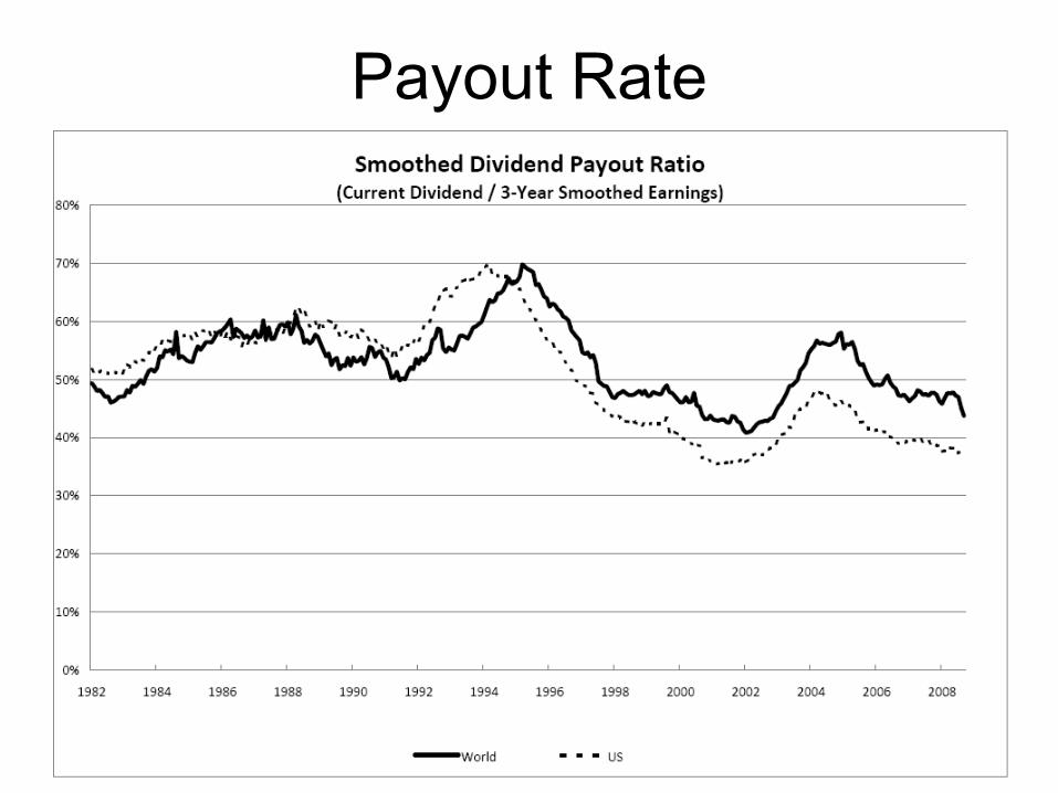
Payout Rate

Real Interest Rate

US Equity Premium

World Equity Premium


�•

If one forecasts ROE and payout with long-run historical average levels, US (world) geometric equity premium was 4.0% (4.6%) at the end of September

�•

Recent ROE data give a much higher and unrealistic number

Comparisons with Other Estimates�•

Dimson, Marsh, and Staunton (2006) report 1900-2005 geometric averages of 5.5% for the US and 4.7% for the world�–

Forward-looking method gives a lower number for the US, but comparable for the world

�•

Graham and Harvey (2007) survey CFO�’s of US corporations and report that the median geometric equity premium forecast in November 2006 was 3.4%


�•

October market decline has increased 3-year smoothed E/P by about 1.4% to 7.8%

�•

This increases the real stock return forecast by about 0.7%

�•

However, the TIPS yield has also increased by about 0.7% in October, so there is little net change in the forecast

�•

Volatility adjustment is about 1.25% in normal times, greater today (VIX2/2

18%!)

New Return Predictors

�•

Finance theory also suggests ways to derive new return predictors from the cross-section of stock prices

�•

Polk-Thompson-Vuolteenaho (JF 2006): �–

If the CAPM is true, a high equity premium implies low prices (value) for stocks with high betas

�–

Equivalently, value stocks should have high betas�–

This was true in the mid-20th

Century, but not today, suggesting a decline in the equity premium

�–

Relative valuations of high-beta stocks can be used to predict the market return.

PTV Cross-Sectional Predictor

PTV predictorSmoothedearnings yield

From CAPM to ICAPM�•

If returns are predictable, then the CAPM does not hold unless investors have log utility

�•

Merton�’s ICAPM says that stocks that covary with declines in the expected market return (�“discount rate news�”) should have lower average returns than stocks that covary with market profitability (�“cash flow news�”), controlling for market beta

�•

The ICAPM can explain the value effect if growth stocks covary more with discount rates than do value stocks

�•

Then past returns on growth stocks, relative to value stocks, should predict the aggregate market return.

From CAPM to ICAPM

�•

The value spread, the relative valuation of value and growth stocks, summarizes the past history of relative returns on these stocks

�•

Eleswarapu and Reinganum (JBusiness 2004) find that the value spread for small stocks predicts the aggregate stock return

�•

Campbell and Vuolteenaho (AER 2004) use the small-stock value spread in a VAR model to estimate and test the ICAPM�–

More on this tomorrow

Cumulative HML return (Jan 1994 Sept 2008)

1.80

0.00

0.20

0.40

0.60

0.80

1.00

1.20

1.40

1.60

1.80

2.00

1994 1995 1996 1997 1998 1999 2000 2001 2002 2003 2004 2005 2006 2007 2008

Cum

ulat

ive

Retu

rn

Current Events

�•

In late 2007 and the first half of 2008,�–

Value stocks underperformed growth stocks

�–

Low-beta stocks fell just as much as high-beta stocks�•

In September and October 2008,�–

Growth stocks underperformed

�–

High-beta stocks did particularly badly�•

The former pattern suggests negative cash flow news (worsening profit outlook)

�•

The latter suggests an increasing equity premium (aka �“panic�”)

Conclusion

�•

Campbell, Lo, and MacKinlay (1997): �–

�“What distinguishes financial economics is the central role that uncertainty plays in both financial theory and its empirical implementation�”

�•

Theory tells us why stock returns are so hard to predict

�•

But it also holds out the promise of better prediction than we can achieve by purely statistical forecasting methods.

Remaining Lectures

�•

Tomorrow I will discuss consumption-based asset pricing models�–

Recent revival of interest

�–

Applications to stocks and real bonds�–

Where is this literature headed?

�•

On Wednesday I will discuss the pricing of nominal Treasury bonds in relation to stocks and real bonds�–

Treasuries as a hedge in the current financial crisis

�–

Extension to currencies



John Y. Campbell

Consumption Risk in Long-Term Asset Markets


November 4, 2008

John Y. Campbell

An E-Z Pass to E-Z Utility


November 4, 2008

John Y. Campbell

Consumption Comeback�•

Consumption-based asset pricing began in the late 1970�’s and early 1980�’s (Breeden 1979, Hansen and Singleton 1982)

�•

Researchers found, studied, and eventually became discouraged by puzzles:�–

Equity premium puzzle

�–

Riskfree rate puzzle�–

Volatility puzzle

�•

Recently, a resurgence of interest building on the richer model of utility proposed by Epstein-

Zin (E-Z 1989)

E-Z Utility

�•

Retains the scale independence of power utility�–

Needed to avoid trends in financial variables as wealth trends upwards

�•

Separates the coefficient of relative risk aversion

from the elasticity of intertemporal substitution

�•

Achieves this by dropping the von Neumann- Morgenstern assumption that people are

indifferent to the timing of the resolution of uncertainty

1Elasticity of Intertemporal Substitution ( )

Constant consumption-wealth ratio

Myopic portfolio choice

Coe

ffic

ient

of R

elat

ive

Ris

k A

vers

ion

()

Log utility

1

Power utility1

E-Z Utility

E-Z Euler Equation

�•

Euler equation can be derived only by assuming a complete-markets budget constraint

�•

Both consumption and wealth return appear in the Euler equation

Two New Models�•

The budget constraint can be used to substitute either wealth or consumption out of the Euler equation

�•

Substituting out wealth (Restoy and Weil 1998) gives a �“CCAPM+�”

model

�–

A particular parameterization with high

and >1 advocated recently by Bansal and Yaron (JF 2004)

�–

�“Long run risks model�”�•

Substituting out consumption (Campbell 1993) gives a �“CAPM+�”

model

�–

An empirical implementation of Merton (1973) ICAPM

Lecture Outline

�•

I will review the CCAPM+ approach and critique the long-run risks model

�•

Then I will turn to the CAPM+ model and apply it to the value effect in stock returns

�•

At the end of the lecture I will speculate about new directions in the literature: �–

Is there still life in the representative agent E-Z paradigm?

�–

How should we model the changing equity premium?�–

What about rare disasters?

�–

What about the current crisis?

Background Research

�•

I will draw on several of my recent papers:�–

�“Consumption-Based Asset Pricing�”, Ch. 13 in Handbook of the Economics of Finance, 2003

�–

�“The Long-Run Risks Model and Aggregate Asset Prices: An Empirical Assessment�”, with Jason Beeler, unpublished, 2008

�–

�“Bad Beta, Good Beta�”, with Tuomo Vuolteenaho, AER 2004

�–

�“Growth or Glamour? Fundamentals and Systematic Risk in Stock Returns�”, with Christopher Polk and Tuomo Vuolteenaho, unpublished, 2008

Loglinear E-Z Euler Equations

�•

Loglinear form of the Euler equations in a homoskedastic model:

Loglinear Budget Constraint

�•

Loglinear return approximation:

�•

For wealth portfolio, d = c, and expected return linear in (1/ ) c:

g

CCAPM+

�•

The risk premium on any asset is determined by its covariances with shocks to�–

contemporaneous consumption (risk price )

�–

long-run consumption growth (risk price -1/ )�•

This is interesting if there are predictable movements in consumption growth

�•

What is the long-run covariance for stock returns?

Levered Equity

�•

Levered equity covaries positively with expected future consumption growth if >1/

�•

Then the CCAPM+ predicts a higher equity premium if >1/

�•

Promising model if

is not too small

Real Bonds

�•

Real (inflation-indexed) bonds have =0�•

They covary negatively with long-run growth (booms raise real interest rates)

�•

Problem: They get a negative term premium if if >1/

Real Bond Yields

Real Bonds

�•

Inflation-indexed bond yields fell dramatically in the 2000�’s, possibly consistent with a negative real term premium

�•

Could this be because of increased uncertainty about long-run growth?�–

Rate of technological progress

�–

Climate change�•

Interestingly, TIPS yields have increased again in the recent crisis (currently at about 3%)

Long-Run Risks Model

�•

The long-run risks model of Bansal and Yaron (BY) adds changing volatility and distinct consumption and dividend processes


�•

BY argue for high risk aversion �•

More controversially, they argue for >1�–

necessary and sufficient for higher consumption volatility to lower the price of consumption claims

�–

necessary for higher consumption volatility to lower the price of dividend claims

�–

strengthens positive stock price response to revisions in expected consumption growth

�–

increases risk premium implied by this response�•

How plausible is this model?


�•

Problem 1: IV estimates of

using comovement of the riskfree rate and consumption deliver values close to zero (Hall 1988)�–

BY point out that the IV regression is misspecified when volatility is time-varying

�–

But this effect is small in simulations of their model �•

Problem 2: Stock prices predict excess stock returns, not consumption or dividend growth�–

CCAPM+ collapses to the traditional CCAPM if there are no predictable movements in consumption growth

Beeler-Campbell 2008

CAPM+

�•

CAPM+ model substitutes consumption out of the E-Z Euler equation, works with wealth�–

Attractive if wealth is better measured than consumption

�–

Does not require predictable movements in consumption growth (these will be small if

is low)

�–

Differs from the traditional CAPM if there are predictable movements in wealth returns

Loglinear Budget Constraint

�•

Loglinear approximation to the budget constraint:

�•

For wealth portfolio, d = c:

h

CAPM+

�•

The risk premium on any asset is determined by its contemporaneous covariance with the market (wealth) return, and its covariance with shocks to future expected market returns

CAPM+

�•

If stock returns mean-revert, then market returns covary negatively with revisions in expected returns�–

This lowers the equity premium for any level of

�–

We need a higher

than traditional CAPM calculation (Friend and Blume AER 1975) would suggest

�–

�“Equity premium puzzle without consumption�” (Campbell JPE 1996)

�•

A more interesting application of the model is to cross-sectional patterns in stock returns

Two Betas and the Value Effect�•

Campbell and Vuolteenaho (2004) rewrite the CAPM+ model in terms of two betas�–

�“Good beta�”

with market discount-rate shocks, risk

price equals market return variance�–

�“Bad beta�”

with market cash-flow shocks, risk price is

times greater

�•

A VAR model for the stock return, including price-smoothed earnings and the value spread as market return predictors, implies that value stocks have higher bad betas but much lower good betas

Two Betas and the Value Effect

�“Good beta�”Risk price 2

M

�“Bad beta�”Risk price 2

M

Campbell-Polk-Vuolteenaho Table 2Aggregate VAR Estimates

Four Betas

�•

Campbell, Polk, and Vuolteenaho (2008) further distinguish cash flow and discount rate news for firms (portfolios), estimating four betas

�•

They find that cross-sectional variation in betas is driven by cash-flow news at the firm (portfolio) level�–

More to �“growth�”

than �“glamour�”

�–

In the technology boom, the equity premium declined and tech stocks had rapid profit growth, not just rising prices

Campbell-Polk-Vuolteenaho Figure 2Beta Patterns in 1929-1962 and 1963-2000

Growth GrowthValue Value

Robustness Concern

�•

Chen and Zhao (RFS forthcoming) argue that these results are not robust to VAR specification

�•

CPV response: �–

Alternative VARs

�–

Direct measurement of firm-level and market-wide cash flows over long horizons

Campbell-Polk-Vuolteenaho AppendixAlternative VAR Systems

CCAPM+ vs. CAPM+

�•

In the short run, wealth is more volatile than consumption

�•

In the long run, these volatilities must be the same

�•

The long-run risks model says consumption is riskier in the long run than in the short run

�•

The two-beta model says wealth is less volatile in the long run than in the short run

�•

In my view the evidence supports the latter

Where Next?

�•

The E-Z representative agent paradigm still has life in it

�•

An obvious next step is to combine information on consumption and wealth �–

Allow for measurement error in each

�–

Impose the cross-sectional restrictions of the model to improve time-series estimation

�•

Structural models of value and growth firms should use the CAPM+, not the CAPM

Where Next?

�•

The paradigm has a serious problem�–

The elephant in the room

�•

It�’s the risk premium that�’s predictable �–

Homoskedastic E-Z model ignores this fact

�–

Long-run risks model tries to capture this with changing volatility, but cannot get enough return predictability

�•

To model this, two possibilities: �–

Changing risk

�–

Changing attitudes towards risk

Changing Risk

�•

Add changing volatility to the CAPM+ model�•

Variable risk of rare disasters (Barro, Weitzman, Gabaix, Wachter)�–

�“Dark matter for economists�”?

�–

It is hard to relate asset prices to reasonable changes in expectations about wars

Changing Attitudes Towards Risk

�•

Habit formation (Campbell-Cochrane 1999) makes risk aversion increase when consumption falls�–

Stochastic volatility models of an exogenous SDF are similar in spirit

�–

Wei Yang (2008) has combined habit formation with E-Z utility and argues for low

�•

Heterogeneous risk aversion has a similar effect�–

Can add participation constraints so that some agents are effectively infinitely risk averse

�–

Then market participants must be leveraged

Limited Participation

�•

Models of limited participation offer rich possibilities�–

Reinterpret habit as the consumption of non-

participants�–

Reinterpret rare disasters as political expropriation of capital owners, not necessarily aggregate consumption disasters

�–

UK 1974

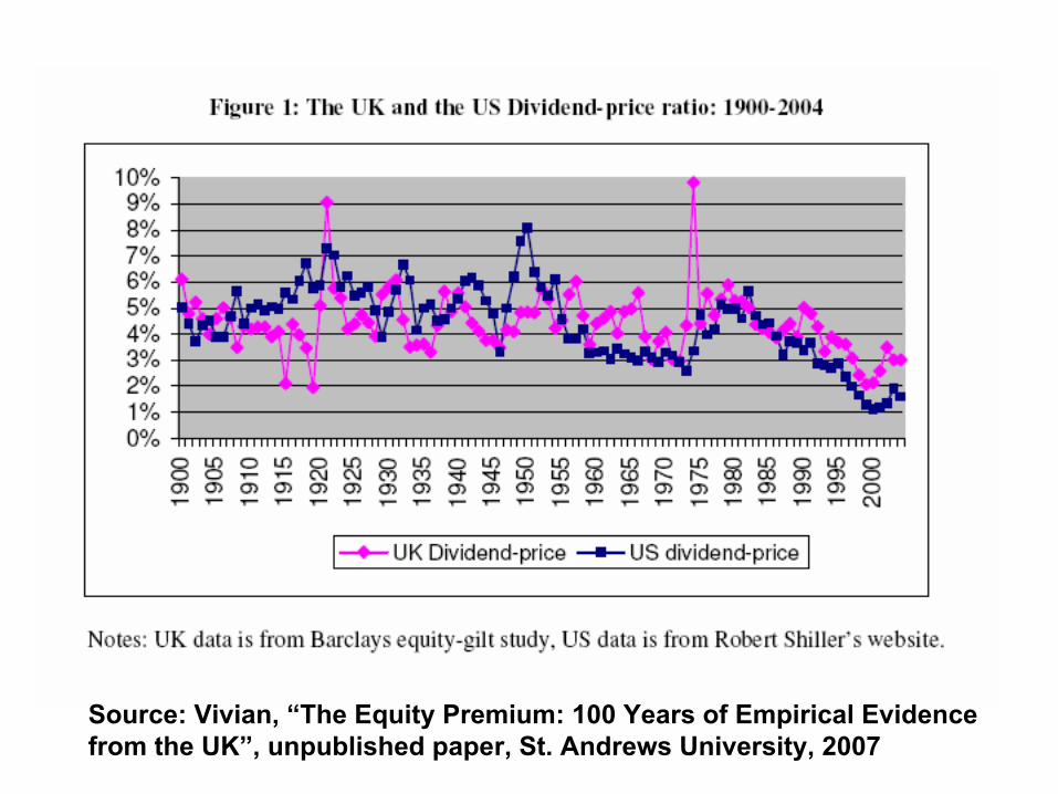
Source: Vivian, �“The Equity Premium: 100 Years of Empirical Evidence from the UK�”, unpublished paper, St. Andrews University, 2007

The UK in 1974

�•

Miners�’

strike, 3-day week, fall of Conservative government

�•

Spike in labor share (Bottazzi, Pesenti, and van Wincoop, EER 1996), and uncertainty about future of UK capitalism

The Current Crisis

�•

How do these models interpret the current drop in stock prices?�–

Long-run risks model: Fall in expected future consumption growth

�–

CAPM+: Decomposition into cash flow news (2007- August 2008) and temporary discount rate increase

(September-October 2008)

The Current Crisis

�•

How do these models interpret the current drop in stock prices?�–

Rare disasters: The probability of a consumption cataclysm has increased

�–

Habit formation: Risk aversion is increasing as consumption falls

�–

Heterogeneous risk aversion: Wealth of risk-tolerant investors is reduced

�–

Political rare disasters: The probability of a consumption cataclysm for stock market investors has increased

Conclusion

�•

Consumption-based models are appealing because they relate asset prices to what investors ultimately care about

�•

They create challenging puzzles�–

Equity premium puzzle is the most famous

�–

Equity volatility puzzle is just as serious�•

We do not have a consumption-based �“model of everything�”�–

But these models have delivered many partial insights

Final Lecture

�•

Tomorrow I will discuss the pricing of nominal Treasury bonds in relation to stocks and real bonds�–

Treasuries as a hedge in the current financial crisis

�–

Extension to currencies



John Y. Campbell

Stocks, Bonds, and the Flight to Quality

Princeton Finance Lecture 3November 5, 2008John Y. Campbell

2

The Panic of 2008�•

What assets have held their value best?�–

US Treasury bills (stable value)

�–

Nominal US Treasury bonds (increasing value)�•

Why have nominal Treasuries been such good hedges?�–

�“Flight to quality�”

helps safe assets, but why are

nominal Treasuries regarded as safe?�–

They have no credit risk, but they do have inflation risk

�•

Have nominal Treasuries always hedged investors against other risks?

3

Understanding Bond Risks�•

This lecture explores time-variation in inflation risk and its effect on the nominal Treasury yield curve

�•

The analysis makes some use of TIPS data but TIPS are not the main focus

�•

At the end, a brief analysis of currencies along the same lines

4

Understanding Bond RisksI draw on several recent pieces of research:�•

Luis Viceira, �“Bond Risk, Bond Return Volatility, and the Term Structure of Interest Rates�”, unpublished, 2007

�•

Campbell, Adi Sunderam, and Viceira, �“Inflation Bets or Deflation Hedges? The Changing Risks of Nominal Bonds�”, unpublished, 2008

�•

Campbell, Karine Serfaty-de Medeiros, and Viceira, �“Global Currency Hedging�”, unpublished, 2008

�•

Campbell, Robert Shiller, and Viceira, research on inflation-indexed bonds, to appear in Brookings Papers on Economic Activity, 2009

5

�•

Speculative motive�–

Higher yields than money market

�•

Hedging motive�–

They do well when other assets decline

�•

At different times, conventional wisdom has emphasized one or the other motive

Why Hold Treasuries?

6

Changing Conventional Wisdom�•

Late 1970�’s and early

1980�’s:

�–

Bonds are exposed to the risk of stagflation�–

Avoid them unless the term premium is high

�•

2000�’s: �–

Bonds are hedges against the risk of deflation

�–

�“Anchor to windward�”�–

Hold them even at a low term premium

�•

Changing

CW reflects

changing reality�–

Bonds as hedges in 2007-2008

7

Luis Viceira, �“Bond Risk, Bond Return Volatility, and the Term Structure of Interest Rates�”, 2007

8

CAPM beta of bonds (2002.06-2008.09)

-0.4

-0.3

-0.2

-0.1

0

0.1

0.2

0.3

06/20

/2002

10/10

/2002

01/30

/2003

05/22

/2003

09/11

/2003

01/01

/2004

04/22

/2004

08/12

/2004

12/02

/2004

03/24

/2005

07/14

/2005

11/03

/2005

02/23

/2006

06/15

/2006

10/05

/2006

01/25

/2007

05/17

/2007

09/06

/2007

12/27

/2007

04/17

/2008

08/07

/2008

Date

CA

PM b

eta

3-month centered beta, 10-year Treasury on S&P500

9

Changing Inflation Behavior�•

The changes in measured bond risks appear to be related to changing behavior of the Phillips Curve

�•

When the Phillips Curve is stable (early 1960�’s, 2000�’s), inflation falls when unemployment rises�–

Then bonds do well in bad times and hedge macroeconomic risk

�•

When the Phillips Curve is unstable (1970�’s and early 1980�’s), inflation and unemployment move together (stagflation)�–

Then bonds do badly in bad times and are risky

10

Stable Phillips Curve

Inflation(-

Rbond)

Unemployment (-

Output)

Good times

Bad times

11

Stable Phillips Curve�•

The Phillips Curve is stable when �–

Supply conditions are stable while demand varies

�–

The public�’s expectations of inflation are stable because the central bank is credible

�•

Downside risk is weak demand�–

Extreme examples: deflation in the US during the Great Depression, in Japan during the 1990�’s

�•

Bonds hedge investors against deflation risk�•

Accordingly, investors are willing to accept low rates of return on bonds

�•

The yield curve tends to be flat�–

An explanation of the �“Greenspan conundrum�”

12

Unstable Phillips Curve

Inflation(-

Rbond)

Unemployment (-

Output)

Bad times

Good times

13

Unstable Phillips Curve�•

The Phillips Curve is unstable when �–

Supply shocks hit the economy

�–

Public expectations of inflation are unstable because the central bank has lost credibility

�•

The downside risk is stagflation�–

Examples: worldwide stagflation of the 1970�’s and early 1980�’s

�•

Bonds fail to protect investors�–

Henry Kaufman, �“Dr. Doom�”

�•

When investors catch on, they demand high rates of return on bonds

�•

The yield curve tends to be steep

14

Modelling

the Yield Curve

�•

How well does this story explain the history of Treasury yields?

15

Luis Viceira, �“Bond Risk, Bond Return Volatility, and the Term Structure of Interest Rates�”, 2007

16

Modelling

the Yield Curve

�•

Changing bond risk does seem to matter over the long run

�•

In the short run, however, there are other influences on the yield curve

�•

To capture its movements, we need to consider more traditional factors as well: �–

The real interest rate

�–

Investor attitudes towards risk�–

Expected

inflation

�•

Campbell, Sunderam, and Viceira 2008 undertakes this project

17

A Bond Pricing Model�•

We consider five factors that move in different ways: �–

Real interest rate xt

(transient) �–

Risk aversion zt

(persistent)�–

Long-run expected inflation t (permanent)

�–

Temporary expected inflation t

(transient)�–

Covariance of inflation with recession t

(persistent, can change sign)

�•

The five factors are not directly observed, so we back out their implied values from data we do observe�–

Nonlinear Kalman

filtering

18

Real Term Structure�•

Real stochastic discount factor (SDF):

�•

xt

is real rate:

�•

zt

drives time-variation in volatility of SDF:

�•

xt

and zt

follow AR(1) processes:

19

Real Term Structure�•

Real (inflation-indexed) term structure is affine in the short-term real interest rate and aggregate risk aversion:

�•

Simple pricing structure, yet risk premium on real bonds varies over time.

20

Risk Premia on Real Assets�•

zt

drives exogenous time-variation in real risk premia.

�•

Real bonds:

�•

Equities:

21

Nominal Term Structure�•

Log inflation (reciprocal of real cash flow on 1-period bonds):

�•

Expected inflation is time-varying, with two components:

�–

Permanent component:

�–

Transitory component:

22


State variable t

follows AR(1) process:

This variable is the main innovation of our model, and plays important role:

�•

( t

)2

drives time variation in the conditional volatility of both realized inflation and expected inflation.

�•

zt t

drives time variation in the covariance of the real economy with inflation, and thus determines nominal bond risk premia.

�•

This covariance (and thus bond risk premia) can switch sign as

t

takes positive or negative values (zt

is always positive in the data)

23


Log nominal SDF:

�•

Log nominal short rate:

�•

The conditional covariance between the real economy (log real SDF) and log inflation determines risk premium on short-term nominal bonds:

Fisher equation Inflation risk premium

24


Nominal term structure is linear-quadratic:

�•

The risk premium on nominal bonds is the real-bond risk premium plus a term in the cross-product zt t

.

25

Nested Models�•

Both zt

and t

constant�–

Two-factor affine yield model of Campbell and Viceira (2001, 2002).

�–

Both real bond risk premia and nominal risk premia are constant.

�•

zt

varying and t

constant�–

Three-factor affine yield model ((Bekaert et al., 2004, Buraschi and Jiltsov 2006, Wachter 2006).

�–

Both real bond risk premia and nominal bond risk premia vary with aggregate risk aversion

�•

zt

constant and t

varying�–

Single-factor affine yield model for the real term structure, and a linear-quadratic model for the term structure for nominal interest rates.

�–

Constant real bond risk premia, time-varying nominal bond risk premia.

26

Estimation

�•

Maximum likelihood via nonlinear Kalman filter because state variables are unobserved.

�•

Unscented Kalman filter (Julier and Uhlmann 1997, Wan and van der Merwe 2000, Koijen and Binsbergen 2008)

27

Observed Variables

�•

Nominal yield curve at maturities 3 months, 1 year, 3 years, 10 years

�•

TIPS yield�•

Realized inflation

�•

Equity returns and dividend yield (proxy for risk aversion)

�•

Realized bond variance and bond-equity covariance in daily data

28

Nominal Yields

29

Real Yields

30

Equity Dividend Yield

31

Bond Second Moments

Bond-Equity Covariance Bond Variance

32

Real State Variables

Real Interest Rate Risk Aversion

33

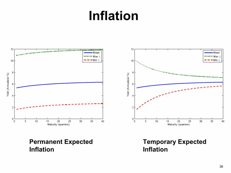
Inflation Components

Permanent Expected Inflation

Temporary Expected Inflation

34

Inflation-Recession Covariance

Stagflation risk

Deflation risk

35

Implications for the Yield Curve

�•

We plot the yield curve at the sample mean of all the state variables

�•

Then we vary each state variable to its sample minimum and maximum, while holding the other state variables at their sample mean

36

Real Interest Rate

Real Yield Curve Nominal Yield Curve

37

Risk Aversion

Real Yield Curve Nominal Yield Curve

38

Inflation

Permanent Expected Inflation

Temporary Expected Inflation

39

Inflation-Recession Covariance

40


�•

Real interest rate and temporary expected inflation move the short end

�•

Risk aversion moves the long end�•

Permanent expected inflation moves the yield curve up and down in parallel

�•

Inflation-recession covariance drives the curvature of the yield curve

41


�•

Fixed-income practitioners analyze the yield curve using level, slope, and curvature factors

�•

They do not relate these factors to external market conditions

�•

Our model does: �–

Real interest rate and permanent

expected inflation

drive

the level factor �–

Real interest rate, risk aversion, and temporary expected inflation drive the slope factor

�–

Inflation-recession covariance drives the curvature factor

42

Implications for Bond Returns

�•

What happens when investors become more risk averse?

�•

If bonds are risky, then investors sell both stocks and bonds

�•

If bonds are hedges, then investors sell stocks and buy bonds (flight to quality)

�•

Thus movements in risk aversion amplify the covariance of bonds and stocks�–

If the covariance is positive, it becomes more positive

�–

If the covariance is negative, it becomes more negative

43

Implications for Term Premia

�•

Expected excess bond returns (term premia) are determined by �–

Price of risk ×

quantity of risk

�–

Risk aversion ×

inflation-recession covariance�–

z ×

�•

Both matter, but the inflation-recession covariance

is more important

44


45


46

Forecasting Bond Returns�•

Both academics and investors are interested in forecasting excess bond returns over bills

�•

Traditional approach, e.g. Campbell and Shiller (1991), is to use the yield spread

�•

Cochrane and Piazzesi

(2005) find a linear combination of interest rates that predicts excess bond returns even better than the yield spread�–

Their measure is roughly the level of the 3-year forward rate relative to the weighted average of 1-

year and 5-year forward rates�–

Thus it captures the curvature of the yield curve

47

Cochrane-Piazzesi

Predictor

48

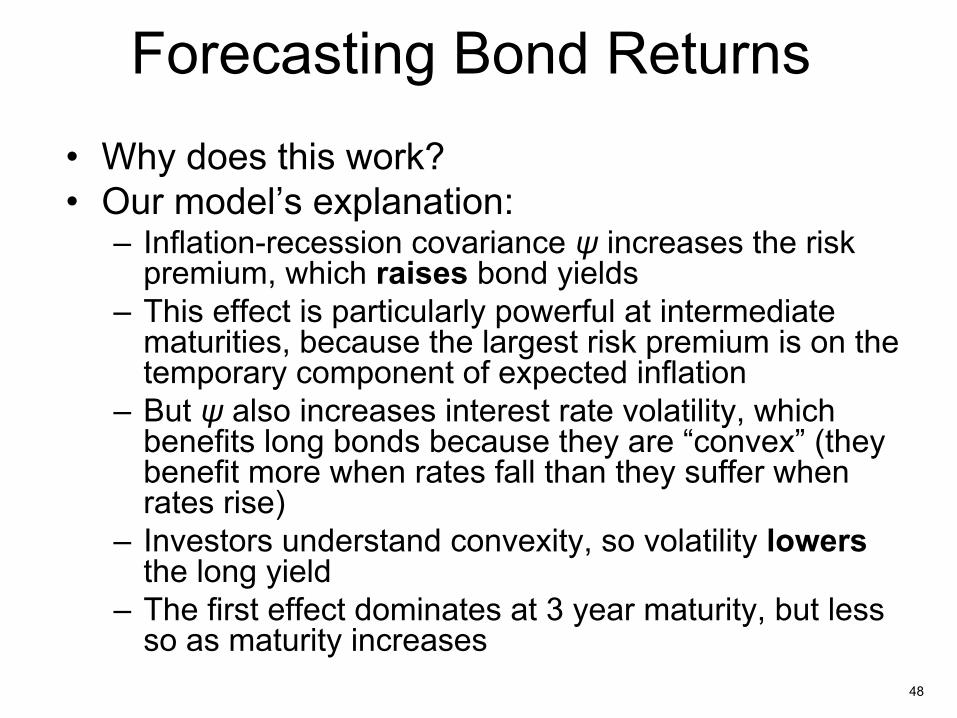
Forecasting Bond Returns�•

Why does this work?

�•

Our model�’s explanation:�–

Inflation-recession covariance

increases the risk

premium, which raises bond yields�–

This effect is particularly powerful at intermediate maturities, because the largest risk premium is on the temporary component of expected inflation

�–

But

also increases interest rate volatility, which benefits long bonds because they are �“convex�”

(they

benefit more when rates fall than they suffer when rates rise)

�–

Investors understand convexity, so volatility lowers the long yield

�–

The first effect dominates at 3 year maturity, but less so as maturity increases

49

The Term Structure Today�•

Investors still trust nominal Treasuries as hedges�–

Little curvature in the Treasury yield curve

�–

Stable and declining long Treasury yields�•

This trust has been well founded recently�–

Treasuries have covaried negatively with stocks over the past year

�–

Panic of 2008 makes inflation procyclical (deflation as the bad outcome)

�•

But what about the future?�–

Energy supply risks remain

�–

New risk of destabilized inflation expectations from expensive financial bailouts

50

What About TIPS?�•

Research in progress with Shiller and Viceira looks at daily variances and covariances of inflation-indexed bonds (TIPS) along with nominal Treasuries

�•

Campbell-Sunderam-Viceira model assumes TIPS-Treasury covariance is time-varying while TIPS-equity covariance is constant

�•

But for most of this decade, the TIPS-Treasury correlation was around 0.9 while the TIPS-equity correlation moved closely with nominal bond-

equity correlation�–

Divergence in September-October 2008

53

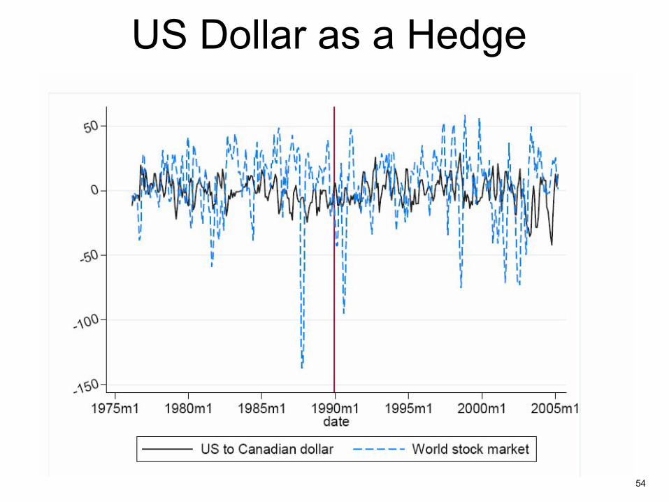
Currency Risks

�•

Campbell, Serfaty-de Medeiros, and Viceira, 2008, show that the US dollar, the euro, and the Swiss franc tended to move against the stock market in the period 1975-2005

�•

The bilateral US-Canadian rate was a particularly good equity hedge

�•

The euro became a better hedge in the second half of the period

54

US Dollar as a Hedge

55

Euro as a Hedge

57

Currencies in 2008Dollar falls on doubts for its safe-haven status.

By Peter Garnham.

The dollar suffered yesterday as coordinated action from global central banks to ease liquidity tension in the world's money markets dented its newly found status as a safe-haven currency. Analysts said the dollar had previously benefited as worries over the state of the global financial system heightened risk aversion, prompting US investors to repatriate funds that had been invested in global equities, while lower inflation expectations had supported demand for US bonds.

"In a world where cross-border equity investing collapses and bond flows remain stable, there is a net inflow back into the dollar", said

Michael Metcalfe of State Street Global Markets.

However, analysts said the decision by global central banks to inject $180bn of emergency dollar liquidity into the market had helped boost risk appetite and damp demand for the dollar.... The dollar's losses were largest against the high-yielding Australian and New Zealand dollars, which had been the worst hit among leading currencies during the recent market turmoil.

Financial Times, September 19, 2008

58

Currencies in 2008

�•

Many of these results hold up during the financial crisis

�•

But the euro has performed worse, and the yen better, than historical patterns predicted

�•

What is driving these patterns?�–

Currencies that are equity hedges are widely used as reserve currencies

�–

They benefit from flight to quality�–

But what are the fundamentals that lead investors to regard them as safe in the first place?

59

Conclusion�•

Asset allocation analysis often assumes stable risks of asset classes

�•

This is a mistake, just as it is a mistake to assume constant expected returns

60

Conclusion�•

Asset class risks change with the macroeconomic environment

�•

The risks of nominal bonds depend on whether deflation or stagflation is the greater threat

�•

Bonds can be used to hedge against deflation, but the hedge fails in stagflation

�•

What will be the risks in the future?

return in stocks and bonds - scholar.harvard.edu · return in stocks and bonds princeton finance...

Documents