284

Revealedpreferences for

redistribution andgovernment’s

elasticityexpectations

Olli Kärkkäinen

� � � � � � � � � � � � � � � � � � � � � � � � � � � � � � � �� � � � � � � � � � � � � � � � � � � � � � � � � � � � � � � � � � ! � � � � � � � � � " � " � � �

# $ % & ' ( ) ' * + , -. / 0 1 2 3 4 0 1 5 6 3 7 8 9 5 5 0 : ; < 3 3 ; = > ? / ; 5 @ A < @ B @ < ? C 9 7 D 0 6 / 0 3 ; 5 5 0 0 1 E F 0 < 3 ; G ; F 0 1 3 6 ; 1 H 0 < ; 7 9 6 6 @ D ; 1 0 < 60 1 E G 7 1 I @ < @ 1 G @ 6 I 7 < 3 4 @ ; < 9 6 @ I 9 = G 7 D D @ 1 3 6 J K B 7 9 = E 0 = 6 7 = ; 5 @ 3 7 3 4 0 1 5 3 4 @ L < M N 8 0 4 1 6 6 7 1 O 7 9 1 E 0 3 ; 7 1 ?3 4 @ P 7 < E ; G C 0 Q R @ 6 @ 0 < G 4 S 7 9 1 G ; = ? T : U : 7 4 M 7 = 0 V < 7 9 F R @ 6 @ 0 < G 4 O 7 9 1 E 0 3 ; 7 1 ? : 0 = 5 0 1 6 0 0 M 0 6 > > 3 ; N 0 1 E3 4 @ O ; 1 1 ; 6 4 W 7 G 3 7 < 0 = : < 7 X < 0 D D @ ; 1 Y G 7 1 7 D ; G 6 I 7 < 3 4 @ ; < Z 1 0 1 G ; 0 = 6 9 F F 7 < 3 J. . [ 1 ; H @ < 6 ; 3 2 7 I C 0 D F @ < @ ? 7 = = ; J 5 0 < 5 5 0 ; 1 @ 1 \ 9 3 0 J Z

] ^ _ ` a ` b c b d ] a e f gh d i j k i i d l m ` a ` b c i e f g` n o p n q r n n s t u q v w v p t x w r o n t v y r` t v p z q r t o o n q { n q v n | a } ~ ~ � | ~ � u o r t q p t` w � � ~ � � e � | � � | | ~i z � p � � y r v t � u v w q t x t � r w p w q t x t � o n � y w { � �� n � y w { d q r v t v w v u � y { b � y q y x t � c u r u n { � �` t v p z q r t o o n q { n q v n | a } � d � ~ ~ � | ~ � u o r t q p t } � t q o n q �] u o u � � y q u � | � f � e � | � � | | ~b � x n t o � � { r v q n x u � r w { q n x u � o n � y w { � �d i � m � � f � � � e � e ~ � � � � g � � � � � � �d i i m � � � � � � f ~ � � � � � �

Tiivistelmä

Tutkimuksessa tarkastellaan Suomen vero- ja sosiaaliturvajärjestelmän taustallavallitsevia tulonjakopreferenssejä. Tämä toteutetaan laskemalla käänteisen opti-miveromallin avulla millä tulonjakopreferensseillä käytössä oleva vero- ja sosiaal-iturvajärjestelmä olisi optimaalinen. Näin estimoidut hyvinvointipainot voidaannähdä tuloeromittarina, joka ottaa huomioon sekä verotuksen tehokkuus- ettätulonjakotavoitteet. Tulokset osoittavat, että Suomen verojärjestelmä voi ollaoptimaalinen vain, jos valtio asettaa hyvin pienen painon pienituloisten työntek-ijöiden hyvinvoinnille. Vuosien 1995 ja 2006 välillä tulonjakopreferenssit ovatmuuttuneet siten, että työttömien suhteelliset hyvinvointipainot ovat laskeneetja työntekijöiden hyvinvointipainot ovat kasvaneet niin, että suurin muutoson tapahtunut pienituloisimmilla työntekijöillä. Muutokset voivat johtua es-imerkiksi aidoista muutoksista suomalaisten tulonjakopreferensseissä, tai muu-toksista valtion arvioissa työn tarjonnan joustosta.

Abstract

This paper examines revealed preferences for redistribution behind the Finnishtax-benefit system in years 1995-2006 using the optimal income taxation frame-work. These implied preferences for redistribution are estimated by solving theredistributive preferences that would make the actual tax-benefit system opti-mal. Revealed preferences for redistribution can be seen as a inequality measurethat takes into account both aspects of the equity-efficiency tradeoff. Whencomparing the redistributive preferences over time a behavioral decompositionmethod is used to separate the mechanical effects due to changes in pre-taxincome from the direct effects of policy changes. Also another dual approach tooptimal income taxation is used in order to estimate the labour supply elasticityexpectations of the government. The results show that the Finnish tax-benefitsystem can be optimal only if the government places a relatively low weight onthe welfare of the working poor. Over a timeperiod when there were severalchanges made to the tax-benefit system that decreased participation tax ratesthere seems to have been a shift of social welfare weight from the unemployed tothe working poor. This shift is mostly due to direct policy changes. There areseveral potential explanations for the change in revealed welfare weights. Oneof them is an actual change in the social preferences for redistribution.

Keywords: Redistribution, inequality, optimal income taxation, social pref-erences

JEL Classification: H11, H21, D63, C63

1 IntroductionThe redistributive preferences of a society can be studied by conducting exper-iments or surveys that measure attitudes towards inequality (e.g. Pirttilä &Uusitalo 2010). Redistributive preferences affect the level of redistribution viatax and transfer programs. The shape of the tax-benefit system is also affectedby labour supply elasticities and the optimal tax system is a balance betweenequity and efficiency.

Optimal income tax models are usually used to estimate optimal marginaltax rates for given labour supply elasticities that maximize some social welfarefunction. By inverting optimal income tax models it is possible to derive therevealed social preferences that make the observed tax-benefit system optimal.This dual approach to optimal taxation has been previously studied in the caseof commodity taxation (e.g. Ahmad & Stern 1984). Inversion of optimal non-linear income tax models was first suggested by Bourguignon & Spadaro (2012)in an application with French data. Bourguignon & Spadaro (2012) invertedboth the Mirrlees model with only intensive labour supply responses and theSaez (2002)’s model with both extensive and intensive labour supply responses.Most of the studies focus on households that have only one adult. This isbecause it is unclear which labour supply elasticities should be used with two-earner households. Bourguignon & Spadaro (2012) focused on single individualswithout children using French data.

Bargain & Keane (2010) focused on single individuals without children usingIrish data from years 1987–2005. Bargain & Keane (2010) tested whether therevealed welfare weights are comparable over time and how the changes in thewelfare weight reflect changes in political forces. Bargain & Keane (2010) foundthat the redistributive preferences of the government did not change much overtime although there were large fiscal reforms and changes in political power.The finding is consistent with the view that the welfare weights reflect the re-distributive preferences of the whole nation and not just the political parties inpower. The results were different for the UK, where the changes in governmenthad a large impact on the welfare weights. Bargain et al. (2013a) compared therevealed inequality aversion in tax-benefit systems of 17 EU-countries (incl. Fin-land) and the US using the revealed redistributive preferences approach. Theyfound that compared to Eastern/Southern Europe the implicit redistributivepreferences in Nordic/Continental Europe are closer to the maximin criterion,where the government only cares about the welfare of the least well-off house-holds. Bargain et al. (2013a) conclude that the high implied inequality aversionin the Nordic countries can be partly caused by differences in the elasticity ex-pectations of governments and the actual labour supply elasticities estimatedfrom the data.

Blundell et al. (2009) compared the social welfare weights of lone mothers inthe UK and Germany. Blundell et al. (2009) found out that in both countriesthe current tax-benefit system is optimal only if the government places much

1

higher weight on the income of the non-workers than those working in low-income jobs. Haan & Wrohlich (2010) extended the analysis of Blundell etal. (2009) by explicitly accounting for the in-kind subsidies of childcare in theGerman tax-benefit system. Haan & Navarro (2008) extended the model to thecollective framework when they compared joint taxation and individual taxationof married couples in Germany.

In the 1990s politicians worried about the so called incentive traps in theFinnish tax-benefit system. Several reforms were made to the Finnish tax-benefit system in order to increase the financial gains from work and reduce thenumber of incentive traps. As a part of the incentive trap reform an in-worktax allowance was introduced to the municipal taxation in 1993. After that theearned income tax allowance in municipal taxation has been increased severaltimes and it is now one of the largest tax allowances in the Finnish tax system.Finland was one of the first countries in Europe to implement an in-work taxcredit that have since become increasingly popular. Because of the incentive trapreforms participation tax rates and effective marginal tax rates have decreasedin Finland. Since the tax-benefit system has changed it is possible that theredistributive preferences of the government have changed as well.

This paper studies changes in the revealed redistributive preferences in Fin-land between 1995 and 2006 by using the inverted Saez (2002) -optimal incometax model. The main interest is to compare the revealed welfare weights of theunemployed and the working poor. Bargain et al. (2013a) estimated that therelative welfare weights of low-income workers are extremely small in Nordiccountries. However in recent years taxation of the working poor has been low-ered in order to account for the high participation elasticities. The changes inthe tax-benefit system might be caused by changes in the elasticity expectationsof the government or the redistributive preferences.

Another contribution of this paper is to use a decomposition approach toseparate the effect of changes in the redistributive preferences from other effects.Policy reforms can be explained by changes in the redistributive preferences andby changes in the pre-tax incomes and demographics. It is possible to separatethese two effects using a decomposition method. The interesting question ishow much of the policy reforms are due to direct changes in the redistribu-tive preferences. Usual microsimulation based decomposition are static in thesense that the “pure policy effect” does not include any behavioral changes.The static decomposition method is therefore not suitable for this study whenthe elasticity expectations of the government are non-zero. Instead a behav-ioral decomposition method is used where the government expectations aboutbehavioral changes due to policy changes are estimated using the elasticity oftaxable income.

The dual approach to optimal income taxation can also be used to estimatethe elasticity estimates that would make the current tax-benefit system opti-mal. The revealed redistributive preferences are found to be non-Paretian forsome years and this may an indication that the elasticity expectations of the

2

government differ from the elasticity estimates taken from economic research.Therefore the dual approach is used to estimate the elasticity expectations thatwould be consistent with the assumption of a Pareto-maximizing social plannerwith given redistributive preferences.

The results show that for given elasticity expectations the Finnish tax-benefitsystem can be optimal only if the government places a relatively low weight onthe welfare of the working poor. If the government does not take participa-tion decisions into account, the relative welfare weight of low-income workersis higher, but still less than the welfare weight of workers with higher wages.However the relative welfare weight of low-income workers has increased between1995 and 2006.

The changes in the tax-benefit system might be also a result from changesin the elasticity expectations of the government. The elasticity expectationswould have to be large and concentrated on middle- and high-income earners inorder for the Finnish tax-benefit system to be optimal for a given social welfarefunction with a modest taste for redistribution.

The paper is organized as follows: Section 2 presents the optimal incometax model. Section 3 describes issues regarding the empirical implementation.Section 4 concentrates on the issues regarding the Finnish tax-benefit system.Section 5 presents the results and finally section 6 concludes.

2 Theoretical background: optimal income taxa-tion (Saez (2002)’s model)

The Saez (2002) model differs from the Mirrlees (1971) optimal tax model inthat it takes into account the participation decision of individuals. In the Saez-model individuals choose whether to work or not and how many hours to work.Individuals choose a consumption-labour -pair that maximizes their utility. So-cial planner maximizes social welfare, which is a function of individual utilities.The social planner can observe only gross incomes and therefore it has to resortto distorting taxation.

2.1 Solving the optimal tax ratesIn Saez (2002)’s model there are I+1 groups in the labour market: I groupswho do work ranked by increasing gross income levels (Yi) and one group whichconsists of those who do not work (Y0 = 0). Individuals choose whether to workor not (the extensive margin) and which group to choose (the intensive margin).In the Saez-model the optimal taxation has the following form:

Ti − Ti−1

Ci − Ci−1=

1

ξihi

I∑j=i

hj

[1− gj − ηj

Tj − T0Cj − C0

], (1)

3

where Ti is the net tax paid by group i, Ci is the disposable income of group i,hi is the share of group i in the whole population and gi are the welfare weightsthat summarize the social preferences of the government. gi is the marginalsocial welfare of a 1€ transfer to an individual in group i expressed in terms ofpublic funds. The mobility elasticity ξi is defined as

ξi =Ci − Ci−1

hi

dhid(Ci − Ci−1)

. (2)

The intensive elasticity captures the percentage increase in group i following a1% increase in Ci − Ci−1 , assuming that individuals can adjust labour supplyonly to the nearest choice. It should be noted that the mobility elasticity differsfrom the classical labour supply elasticity, εi which measures the effects of wageson hours of work in a continuous case.

The extensive elasticity ηi is defined as

ηi =Ci − C0

hi

dhid(Ci − C0)

. (3)

The participation elasticity measures the percentage of individuals in group iwho stop working when the difference between the disposable income out of workand at earnings point i is decreased by 1%. It should be noted that for group 1the participation elasticity is equal to the mobility elasticity by definition. It ispossible to study pure intensive or pure extensive models by setting either theparticipation elasticity or the mobility elasticity to zero for all groups.

When there are no income effects the welfare weights can be normalized bythe following constraint: ∑

i

higi = 1. (4)

The government budget constraint restricts that the sum of net taxes has toequal the consumption of the government,∑

i

hiTi = H. (5)

2.2 Solving the revealed welfare weightsThe optimal tax schedule can be calculated from (1) under assumptions on theelasticities and social preferences. Equation (1) can be inverted to calculatethe welfare weights for which the current tax-benefit schedule is optimal. Theinversion is straightforward. From (1) we obtain that for i = 1, . . . , I − 1

gi = 1− ηiTi − T0Ci − C0

− ξiTi − Ti−1

Ci − Ci−1+

1

hi

I∑j=i+1

hj

[1− gj − ηi

Tj − T0Cj − C0

]. (6)

4

For group I the welfare weight is

gI = 1− ηITI − T0CI − C0

− ξITI − TI−1

CI − CI−1. (7)

Using the normalization condition (4) together with (6) and (7) yields the wel-fare weight for the non-working group:

g0 =1

h0

(1−

I∑i=1

higi

). (8)

2.3 Solving the revealed elasticity expectations

Equation (1) can also be used to solve the elasticities that would make thecurrent tax-benefit system optimal for given welfare weights. The elasticityexpectations are calculated separately for a pure extensive model, pure intensivemodel and a model with both intensive and extensive labour supply responses.For a pure extensive model the revealed participation elasticity expectations forgroups i = 1, . . . , I are

ηi =Ci − C0

Ti − T0(1− gi). (9)

For the pure intensive model the revealed mobility elasticity expectationsfor groups i = 1, . . . , I are

ξi =Ci − Ci−1

Ti − Ti−1

1

hi

I∑j=i

hj(1− gj). (10)

For a model with both extensive and intensive labour supply responses, theparticipation elasticity expectations with given mobility elasticities for groupsi = 2, . . . , I − 1 are

ηi =Ci − C0

Ti − T0[1− gi − ξi

Ti − Ti−1

Ci − Ci−1+

1

hi

I∑j=i+1

hj(1− gj − ηjTj − T0Cj − C0

)]. (11)

For group I the revealed participation elasticity is

ηI =CI − C0

TI − T0[1− gI − ξI

TI − TI−1

CI − CI−1]. (12)

Finally for group 1 the mobility elasticity and participation elasticity areequal by definition and therefore the revealed participation/mobility elasticityfor group 1 is

η1 =C1 − C0

2(T1 − T0)[1− g1 +

1

h1

I∑j=2

hj(1− gj − ηjTj − T0Cj − C0

)]. (13)

5

3 Empirical implementation

3.1 Calculating the welfare weights

The marginal welfare weights can be computed from equations (6), (7) and(8) using the observation of Ti, Ci, hi, ξi and ηi for each i = 0, . . . , I. Theinformation about net taxes Ti and disposable income Ci is usually found in thedata or they can be calculated using a microsimulation model and informationabout the gross labour income Yi = Ci + Ti . Bourguignon & Spadaro (2012)discussed the assumptions that have to hold in order for the inversion to bemeaningful. One of them is that the revealed social welfare function has tobe non-decreasing everywhere. Negative welfare weights for some groups wouldviolate this assumption about a Paretian welfare maximizing social planner.

Observed labour supply behavior to tax-benefit reforms is a function of trueelasticities. Observed tax-benefit policies are instead a function of the elasticityexpectations of policy makers. The expectations of policy makers can differfrom true elasticities especially if the elasticities change over time. The elas-ticity expectations should be used when estimating the revealed redistributivepreferences of policy makers. Since these values are not known, they have tobe estimated. The elasticities can be estimated from the data assuming thatthe elasticity expectations are the same as true elasticities (e.g. Blundell et al.2009; Bargain & Keane 2010; Bargain et al. 2013a). Another way of estimatingthe elasticity expectations is to the upper and lower bounds for the elasticitiesbased on previous research results (e.g. Bourguignon & Spadaro 2012; Spadaroet al. 2012). The assumption in this case is that research on labour supplybehavior influences the elasticity expectations of policy makers. There are alsoother possible ways of estimating the elasticity expectations of the government.Information about the expected labour supply responses can be possibly foundin the government proposals for amendments to tax legislation. If the govern-ment uses a behavioral microsimulation model when estimating the impacts oftax-benefit reforms, the elasticity estimates used in these simulations would bethe best estimates for the government’s elasticity expectations.

Almost all of the studies focus only on one demographic group at a time. Thisrequires the assumption that the redistribution between different demographicgroups and within a group is separable. The focus in the studies is on thevertical redistribution within a single homogenous group. The redistributionbetween groups is assumed to be constant and therefore the sum of net taxes inthe government budget constraint can be negative for some demographic groups(e.g. single parents).

6

3.2 Decomposition approach

The income distribution is affected by policy reforms and changes in the demo-graphics and pre-tax wages. Using a decomposition approach it is possible toseparate the direct effect of policy changes from other factors. When comparingthe changes is the welfare weights over time it is interesting to see how muchof the changes can be explained with direct effects of policy reforms. The de-composition approach is usually used with different inequality measures. Thestructure of revealed welfare weights can be seen as an inequality measure thattakes into account the efficiency aspect in the shape of tax-benefit systems.

The decomposition method is based on the microsimulation assisted decom-position approach used in Bargain & Callan (2010) and Bargain et al. (2013b).Consider a matrix y that includes information about individuals’ pre-tax in-come from different sources and socio-demographic characteristics that affecttax-benefit calculations. Tax-benefit function d represents the rules and struc-tures of the tax-benefit system (e.g. marginal tax rates). The tax-benefit calcu-lations also depend on a set of monetary parameters (e.g. threshold level of taxbrackets) p. Gross income is transformed into disposable income with the func-tion di(pj, yl) using population from year l, tax-benefit structure from year i andtax-benefit parameters from year j. The income levels and/or parameters p canbe nominally adjusted using factor α. For example dt(αt+1pt, yt+1)calculatesdisposable incomes using population from year t+1, tax rules from year t, andparameters from year t that are nominally corrected using factor αt+1. (Bargainet al. 2013b)

The total change in the distribution of disposable income (or in this case thedistribution of welfare weights) is characterized as

4 = G[dt+1(pt+1, yt+1)]−G[dt(pt, yt)]. (14)

The total change can be decomposed between the contribution of policy re-forms and the “other” effect caused changes in pre-tax wages and demographics.

4 = {G[dt+1(pt+1, yt+1)]−G[dt(αt+1pt, yt+1)]} (policy effect)

+ {G[dt(αt+1pt, yt+1)]−G[dt(p

t, yt)]} (other effect) (15)

It should be noted that the nominally adjusted parameters αt+1pt are notidentical to the actual parameters pt+1 decided by the policy makers. Thereforethe policy effect includes both the effect of changes in the tax-benefit structure(dt to dt+1) and the effect of adjusting the policy parameters (pt to pt+1) whenthe adjustment differs from a plain nominal adjustment with factor αt+1 (e.g.price inflation or earnings growth). The counterfactual simulations needed forthe decomposition are calculated using a microsimulation model.

7

The described decomposition method is static in the sense that all behavioralresponses to tax-benefit changes are included in the other effects and the policyeffects are static changes to inequality measures due to policy changes. Thestatic decomposition method is not directly suitable for decomposing changesin the revealed redistributive preferences when the government expects policychanges to have impacts on labour supply. Instead the policy effect should in-clude the expectations of the government about the behavioral effects of policychanges. Bargain (2012) used labour supply simulations to decompose changesin income distributions to policy effects, other effects and behavioral effects.The other effect in (15) can be divided into behavioral effects and other effects.Denote yt+1

t population of year t+1 making labour supply decisions using thetax-benefit policies of year t. Now the total change in the distribution of dis-posable income can be decomposed between the static policy effects, behavioraleffects and other effects.

4 = {G[dt+1(pt+1, yt+1)]−G[dt(αt+1pt, yt+1)]} (policy effect)

+ {G[dt(αt+1pt, yt+1)]−G[dt(α

t+1pt, yt+1t )]} (behavioral effect)

+ {G[dt(αt+1pt, yt+1

t )]−G[dt(pt, yt)]} (other effect) (16)

One possible way of estimating behavioral effects of tax reforms is to use theelasticity of taxable income. In addition to pure labour supply responses, theelasticity of taxable income (ETI) can also capture other margins of adjustment(f.e. tax planning). The elasticity of taxable income is defined as

ETI =1− τz· ∂z

∂z(1− τ),

where z is the reported income of the individual and τ is the marginal taxrate. Elasticity of taxable income is defined as the percentage change in reportedincome when the net-of-tax-rate increases by 1 percent. (Saez et al. 2012.)

When decomposing the changes in revealed redistributive preferences thepolicy effect with expected labour supply responses is the sum of the first twoelements in (16). Using the elasticity of taxable income and true changes inmarginal tax rates the policy effect with expected behavioral responses can bedefined as

G[dt+1(pt+1, yt+1)]−G[dt(αt+1pt, (1 + ETI

τt − τt+1

1− τt+1)yt+1)].

8

3.3 Calculating the revealed elasticity expectations

The revealed elasticity expectations can be calculated from equations (9) - (13)using information about net-taxes, disposable incomes and redistributive pref-erences of the government. The welfare weights are calibrated in the same wayas in Saez (2002). The curve of the marginal welfare weights is g(c) = 1/(p · cv),where v is a parameter defining the redistributive tastes of the government andp denotes marginal value of public funds, calibrated to satisfy equation (4). Re-distributive tastes increase with v and redistributive preferences of a maximincriterion can be obtained by setting v = +∞. The calculations are done usingdifferent redistributive tastes.

The elasticities are calculated separately using a pure intensive model, pureextensive model and a model with both extensive and intensive responses. Whenthere are both intensive and extensive labour supply responses the participationelasticity expectations are calculated taking the mobility elasticity estimates asgiven for groups i = 2, . . . , I.

9

4 Estimating the revealed preferences for redis-tribution in Finland

4.1 Data and estimation methods

The empirical estimation is based on a panel data from 1995 to 2006. The dataconsists of 30 000 individuals per year. The register based data has informationon the gross income, net taxes and disposable income of the households. Thedata also has information on the labour supply of the individuals.

The welfare weights can be computed using the register data or by using amicrosimulation model to estimate the taxes and social transfers for each incomegroup.

Income groups

The study focuses on childless individuals aged between 20 and 64 years. Stu-dents and pensioners are excluded from the sample. Also households wherecapital income represents more than 10% of total gross income are excludedfrom the sample. The selected sample size is between 600 and 2000 dependingon the year.

The sample is divided into 6 groups. The partitioning of the population canbe done in different ways. The simplest way is to use income quintiles (e.g.Bargain et al. 2013a; Blundell et al. 2009). When using income quintiles, group0 consists of households with no or very little labour income. The 5 other groupsconsist of income quintiles among workers. Another possibility is to partitionthe population into groups by using the median income in each year. Spadaro etal. (2012) defined income groups in different countries using information aboutthe median income and minimum wage (60% of median income). Group 1 startsat half the minimum wage and group 2 at 1.3 times the minimum wage. Group3 starts at the median income and group 4 at 1.5 times the median income.Finally group 5 starts at twice the median income.

In this research the population is partitioned using income quintiles andinformation about the median wage. Group 0 consists of those with wage incomeless than 30 % of the median wage income. The rest of the groups are simplyincome quintiles among the rest of the population.

Unemployment benefits

Should the unemployment benefits be treated as redistributive social assistanceor as delayed salary? Most of the previous studies have treated unemploymentbenefits as replacement income and therefore persons who receive unemploymentbenefits have been treated as workers.

In Finland the unemployment benefits are partly linked to workers pastearnings. Persons who are not eligible for earnings related unemployment benefit

10

receive a basic unemployment allowance or labour market subsidy that is notlinked to past earnings. The requirement for earnings related unemploymentallowance are met if the person has been a member of a unemployment fund priorto the unemployment and meets the employment requirement. The employmentrequirement is met if the person has been employed for at least 34 weeks in the28 months preceding the date of registering as an unemployed job seeker. Theearnings related unemployment allowance consists of a basic component and anearnings-related component. The basic component is the same as in the basicunemployment allowance. The earnings related component depends on the wagebefore the unemployment.

The basic component is the same for all unemployed persons with the samenumber of children and is not linked to past earnings. Therefore the basic com-ponent could be seen as a redistributive assistance for the unemployed. Theearnings related part on the other hand could be seen as delayed salary. Unfor-tunately the dataset has only information about the earnings related unemploy-ment benefit as whole and it is not possible to divide the unemployment benefitbetween the basic component and the earnings related component.

In the basic setting both the basic unemployment allowance and the earningsrelated unemployment allowance are treated as a redistributive benefit.

Elasticity estimates

The estimates for the elasticity of labour supply are taken from previous research(Bargain & Orsini 2006). In the basic setting the extensive (ηi) elasticity is as-sumed to be 0.25. The mobility elasticities estimates (ξi) for groups 2-5 rangingfrom 0.02 to 0.05 are taken from Bargain et al. (2013a) while the mobility elas-ticity of group 1 is equal to the extensive elasticity by definition. Sensitivityanalysis is conducted by testing other values for the elasticity estimates.

11

4.2 Changes in the Finnish tax-benefit system between1995 and 2006

In the optimal income taxation framework the changes in the tax-benefit sys-tem are responses to changes in the social welfare weights, the labour supplyelasticities or the distribution of pre-tax income.

Several policy changes were made to the Finnish tax-benefit system between1995 and 2006 that increased the financial gains from work. If the labour supplyelasticities have not changed, then there should be a change in the relativewelfare weights of groups 0 (unemployed) and 1 (working poor).

In-work tax allowances were introduced to the Finnish tax-benefit systemin the 1990s “incentive trap reforms”. The largest in-work tax allowance is theearned income allowance in municipal taxation. The allowance was increasedseveral times between 1995 and 2006. The maximum deduction from taxableincome was 2000 FIM (ca. 350€) in 1995. In 2006 the maximum deduction fromtaxable income was 3850€. In addition to the increases in the earned incometax allowance in municipal taxation a new in-work credit was implemented tostate taxation in 2006. In 2006 the earned income allowance in state taxationdeducts a maximum of 157 € from paid taxes.

While the low-income tax allowances were increased, the nominal adjustmentfor social transfers to the unemployed was slow between 1995 and 2006. Theincrease in low-income allowances and the slow adjustment of social transfersincrease the financial gains from low-income work. Therefore they affect thegap in welfare weights of groups 0 and 1.

12

5 Results

5.1 Descriptive statistics

The descriptive statistics for years 1995, 2001 and 2006 are found in Table 1.Group 0 consists of those with wage income less than 30 % of the median wageincome. The rest of the groups are simply income quintiles among the rest of thepopulation. Table 1 has information about the average wage income, disposableincome and size of each income group. The incomes are in Euro per year. Thegross wage income has increased in all income groups between 1995 and 2006.

Table 1: Descriptive statistics

Income groups 1995 2001 2006

Wage income (Yi)

0 1134 1214 17161 10920 13739 152932 17063 20436 228473 20040 24299 269924 24265 29166 325685 34586 42226 48300

Disposable income (Ci)

0 7570 7963 91191 10063 12148 139522 12187 15329 178283 13765 17439 202824 16011 20355 235945 20737 27102 32111

Group size (hi)

0 22,75 % 18,57 % 16,68 %1 15,57 % 16,35 % 16,68 %2 15,37 % 16,25 % 16,68 %3 15,57 % 16,35 % 16,64 %4 15,37 % 16,25 % 16,68 %5 15,37 % 16,25 % 16,64 %

All incomes in € / year

13

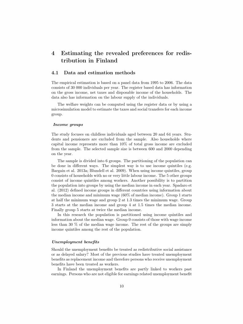
Discrete effective marginal tax rates (Ti − Ti−1)/(Yi − Y i−1) were also cal-culated. The discrete effective marginal tax rate is not precisely a marginaltax rate since the income change to the neighboring group is larger than in thenormal marginal case (e.g. 1 % increase in income). For group 1 the discreteeffective marginal tax rate is actually a participation tax rate since the neigh-boring group is the non-working group. The results for years 1995 and 2006can be found in Figure 1. The figure is U-shaped in both years. Participationtax rates are quite high in both years. The effective marginal tax rates havedecreased in all income groups between 1995 and 2006. The largest change wasin group 2.

0.2

.4.6

.81

1 2 3 4 5Group

EMTR: 2006 EMTR: 1995

Figure 1: Discrete effective marginal tax rate (EMTR), years 1995 and 2006

14

5.2 Revealed redistributive preferences

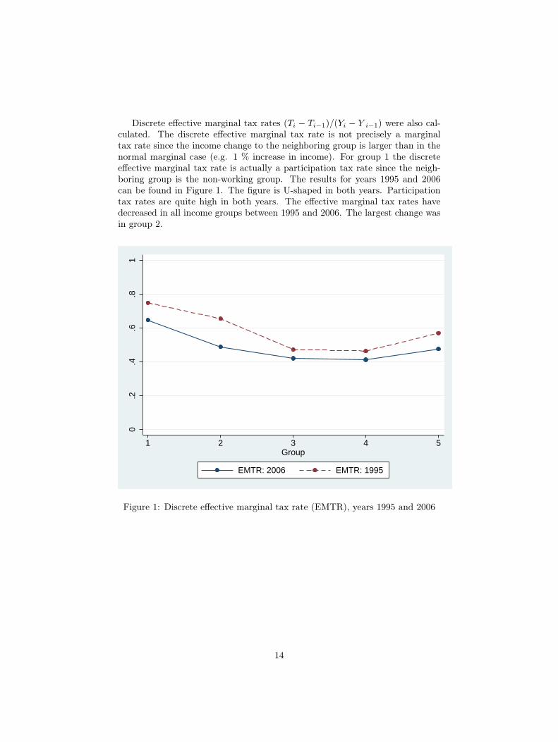
The welfare weights for childless individuals were calculated separately for eachyear using (6), (7) and (8). The welfare weights for each income group in 2006are found in Figure 2. All welfare weights are positive, so they are consistentwith the assumption of a Paretian social planner. The largest welfare weight isplaced on the poorest group. However the welfare weights are not monotonicallydecreasing. The welfare weight of group 1 is much smaller than the welfareweights of groups with higher wage income. This means that the social welfarewould increase by redistributing from the low-income earners to high-incomeearners. The small welfare weight of group 1 is due to high participation taxrates. If the participation elasticity is significant, then the high participationtax rate can be optimal only if the welfare weight of the working poor is verysmall. The welfare weight of group 1 could be increased by adding more in-worktype benefits to the working poor.

01

23

Wel

fare

wei

ght (

g)

0 1 2 3 4 5Group

Figure 2: Welfare weights, year 2006

15

The elasticity estimates have a large impact on the welfare weights. The re-vealed welfare weights in 2006 with different estimates for the extensive elasticityare found in Figure 3. With a pure intensive model (ηi = 0), the shape of thewelfare weights is close to utilitarian preferences. However the welfare weightof group 1 is still smaller than the welfare weight of other income groups. If theparticipation elasticities are very high (ηi = 0.5) the welfare weight of group 1is negative. So with very high participation elasticities the welfare weights arenot consistent with the assumption of a Paretian social planner.

−2

02

46

Wel

fare

wei

ght (

g)

0 1 2 3 4 5Group

2006: e=0.25 2006: e=0 (pure intensive model)2006: e=0.5

Figure 3: Welfare weights with different estimates for extensive elasticity

Additional robustness checks regarding the role of earnings related unem-ployment benefit and the definition of income groups were also done. Theresults are in the Appendix.

16

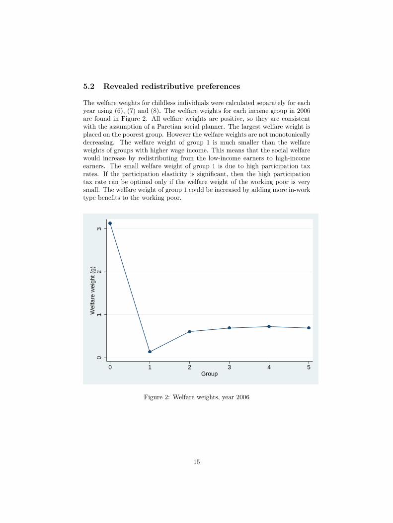
5.3 Changes in the redistributive preferences between 1995and 2006

In order to estimate how the redistributive preferences have changed over time,the welfare weights were calculated also for years 1995 and 2001. To aid thecomparison between years, the welfare weights are expressed relative to thewelfare weight of group 0. The relative welfare weights are found in Figure4. First thing to notice from the figure is that the welfare weight of group 1 isnegative in 1995. This is not consistent with the assumption of a Paretian socialplanner. Negative welfare weights mean that redistribution to the working poorwould actually decrease social welfare.

The relative welfare weights of groups 1–5 have all increased between 1995and 2006. The largest change is found in groups 1 and 2. The overall structureof the relative welfare weights has changed so that the dip in the welfare weightof group 1 is smaller in 2006 than in 1995. The change in the relative welfareweights is much larger between 1995 and 2001 than between 2001 and 2006.

0.5

1R

elat

ive

wel

fare

wei

ght g

(i)/g

(0)

0 1 2 3 4 5Group

2006 19952001

Figure 4: Relative welfare weights: years 1995, 2001 and 2006

It should be noted that the elasticity estimates have a large impact on theestimated welfare weights. The relative welfare weights in Figure 4 were cal-culated with the assumption that the elasticity estimates have not changed

17

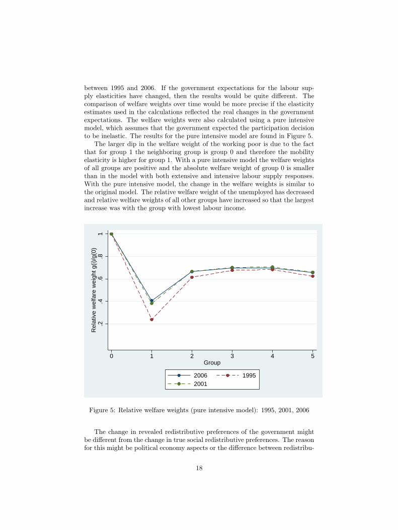
between 1995 and 2006. If the government expectations for the labour sup-ply elasticities have changed, then the results would be quite different. Thecomparison of welfare weights over time would be more precise if the elasticityestimates used in the calculations reflected the real changes in the governmentexpectations. The welfare weights were also calculated using a pure intensivemodel, which assumes that the government expected the participation decisionto be inelastic. The results for the pure intensive model are found in Figure 5.

The larger dip in the welfare weight of the working poor is due to the factthat for group 1 the neighboring group is group 0 and therefore the mobilityelasticity is higher for group 1. With a pure intensive model the welfare weightsof all groups are positive and the absolute welfare weight of group 0 is smallerthan in the model with both extensive and intensive labour supply responses.With the pure intensive model, the change in the welfare weights is similar tothe original model. The relative welfare weight of the unemployed has decreasedand relative welfare weights of all other groups have increased so that the largestincrease was with the group with lowest labour income.

.2.4

.6.8

1R

elat

ive

wel

fare

wei

ght g

(i)/g

(0)

0 1 2 3 4 5Group

2006 19952001

Figure 5: Relative welfare weights (pure intensive model): 1995, 2001, 2006

The change in revealed redistributive preferences of the government mightbe different from the change in true social redistributive preferences. The reasonfor this might be political economy aspects or the difference between redistribu-

18

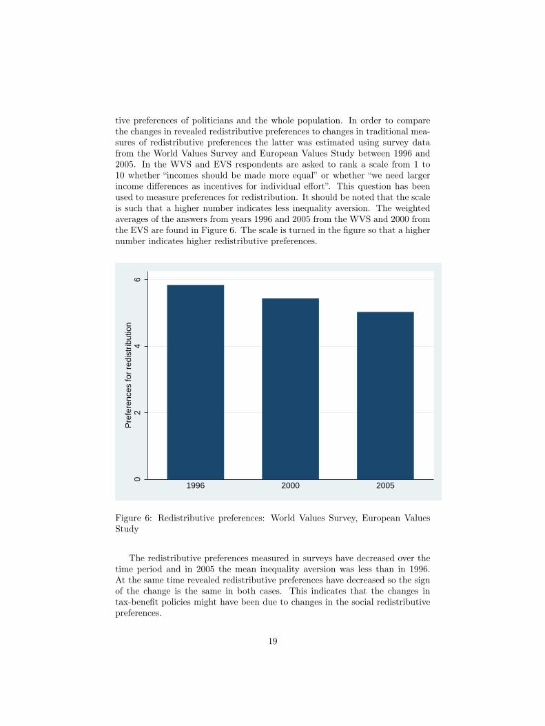
tive preferences of politicians and the whole population. In order to comparethe changes in revealed redistributive preferences to changes in traditional mea-sures of redistributive preferences the latter was estimated using survey datafrom the World Values Survey and European Values Study between 1996 and2005. In the WVS and EVS respondents are asked to rank a scale from 1 to10 whether “incomes should be made more equal” or whether “we need largerincome differences as incentives for individual effort”. This question has beenused to measure preferences for redistribution. It should be noted that the scaleis such that a higher number indicates less inequality aversion. The weightedaverages of the answers from years 1996 and 2005 from the WVS and 2000 fromthe EVS are found in Figure 6. The scale is turned in the figure so that a highernumber indicates higher redistributive preferences.

02

46

Pre

fere

nces

for

redi

strib

utio

n

1996 2000 2005

Figure 6: Redistributive preferences: World Values Survey, European ValuesStudy

The redistributive preferences measured in surveys have decreased over thetime period and in 2005 the mean inequality aversion was less than in 1996.At the same time revealed redistributive preferences have decreased so the signof the change is the same in both cases. This indicates that the changes intax-benefit policies might have been due to changes in the social redistributivepreferences.

19

5.4 Decomposition results

The data set does not have a microsimulation model linked to it. Thereforethe estimations about the direct effect of policy reforms are done using differ-ent data. The data is from the Finnish Income Distribution Survey that isused in JUTTA microsimulation model. The data consists of 30 000 individualsper year. JUTTA is a static microsimulation model developed as a coopera-tive effort between the Labour Institute for Economics Research, Åbo AkademiUniversity and the Research Department of Finnish Social Insurance Institu-tion. It encompasses Finnish social security and personal tax legislation for allthe years needed in the decomposition. The welfare weights calculated withthe microsimulation model and legislation from year 2006 are extremely closeto the ones calculated with the register based data set (Appendix). Thereforethe JUTTA model and its data are used when conducting the decompositionestimation.

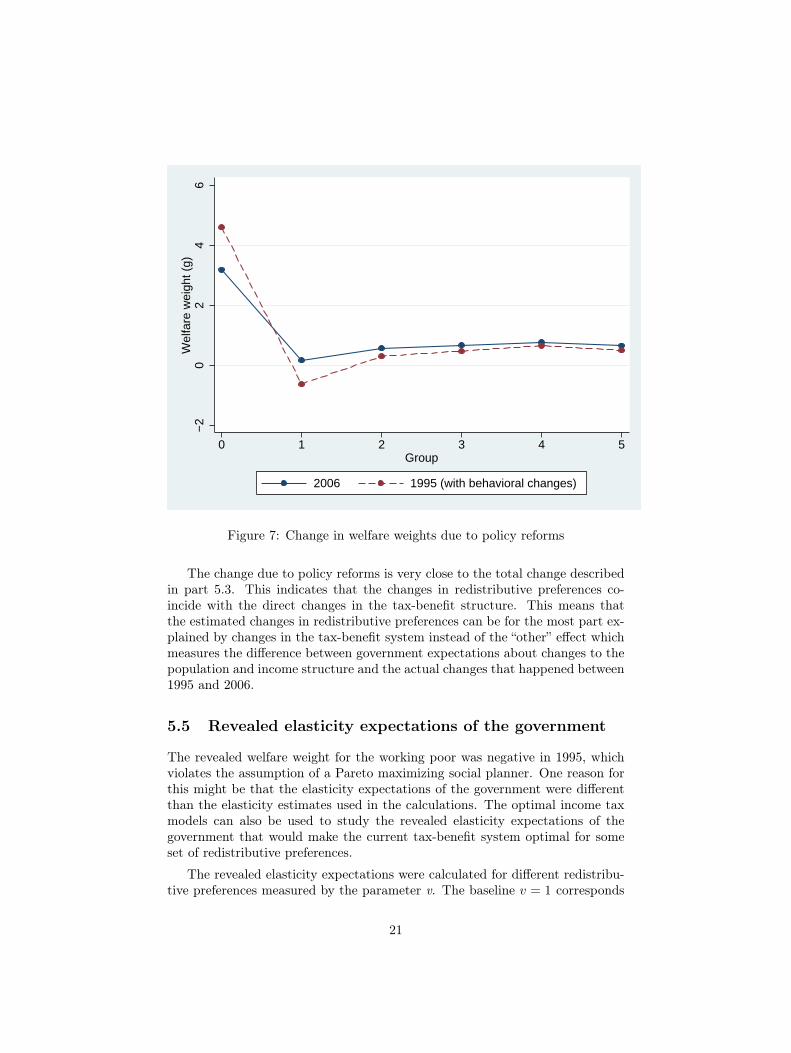
The decomposition results were estimated using end period data (2006).Usually the decomposition is calculated as an average of the results from usingend period data and base-period data. In this case the microsimulation modeldoes not have data from the base-period (1995). Both Bargain & Callan (2010)and Bargain et al. (2013b) found that the results from using only base- orend period data were very close to the average results and they concluded thatwhen necessary estimations can be done with only base- or end period data.The direct effects of policy reforms were estimated by using data from 2006 andtax-benefit structure from 1995. The tax-benefit parameters were nominallyadjusted using changes in the consumer price index. The expected behavioraleffects were estimated by calculating marginal tax rates in both years and usingelasticity of taxable income to estimate the behavioral responses. The estimatefor the elasticity of taxable income used in the calculations was 0.20.

The results from the simulations are found in Figure 7. Since the populationis the same in all simulations, the comparison is done using absolute welfareweights. Between 1995 and 2006 the welfare weights of unemployed have de-creased and the welfare weights of all other groups have increased. The largestincrease was in groups 1 and 2. These changes are directly due to policy reformswithout changes in the population or income structure. These changes includethe government expectations about behavioral responses to tax-benefit reforms.The overall structure of the welfare weights changed such that the relative wel-fare weight of the working poor increased and the dip in their welfare weightwas smaller in 2006.

20

−2

02

46

Wel

fare

wei

ght (

g)

0 1 2 3 4 5Group

2006 1995 (with behavioral changes)

Figure 7: Change in welfare weights due to policy reforms

The change due to policy reforms is very close to the total change describedin part 5.3. This indicates that the changes in redistributive preferences co-incide with the direct changes in the tax-benefit structure. This means thatthe estimated changes in redistributive preferences can be for the most part ex-plained by changes in the tax-benefit system instead of the “other” effect whichmeasures the difference between government expectations about changes to thepopulation and income structure and the actual changes that happened between1995 and 2006.

5.5 Revealed elasticity expectations of the government

The revealed welfare weight for the working poor was negative in 1995, whichviolates the assumption of a Pareto maximizing social planner. One reason forthis might be that the elasticity expectations of the government were differentthan the elasticity estimates used in the calculations. The optimal income taxmodels can also be used to study the revealed elasticity expectations of thegovernment that would make the current tax-benefit system optimal for someset of redistributive preferences.

The revealed elasticity expectations were calculated for different redistribu-tive preferences measured by the parameter v. The baseline v = 1 corresponds

21

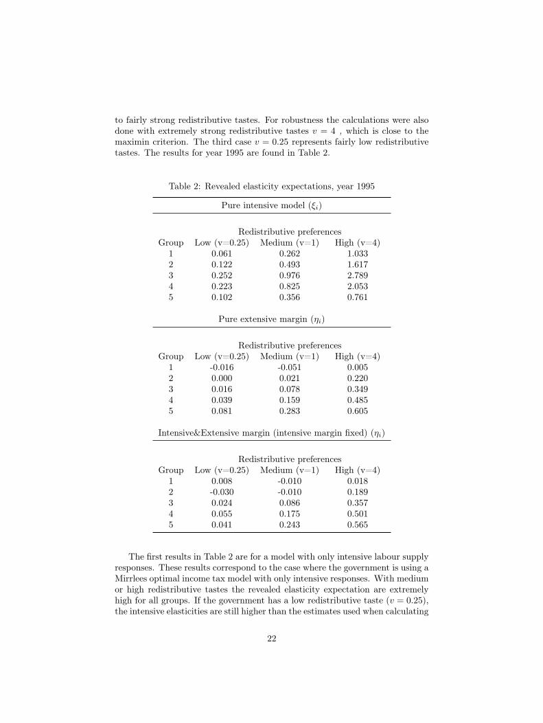
to fairly strong redistributive tastes. For robustness the calculations were alsodone with extremely strong redistributive tastes v = 4 , which is close to themaximin criterion. The third case v = 0.25 represents fairly low redistributivetastes. The results for year 1995 are found in Table 2.

Table 2: Revealed elasticity expectations, year 1995

Pure intensive model (ξi)

Redistributive preferencesGroup Low (v=0.25) Medium (v=1) High (v=4)

1 0.061 0.262 1.0332 0.122 0.493 1.6173 0.252 0.976 2.7894 0.223 0.825 2.0535 0.102 0.356 0.761

Pure extensive margin (ηi)

Redistributive preferencesGroup Low (v=0.25) Medium (v=1) High (v=4)

1 -0.016 -0.051 0.0052 0.000 0.021 0.2203 0.016 0.078 0.3494 0.039 0.159 0.4855 0.081 0.283 0.605

Intensive&Extensive margin (intensive margin fixed) (ηi)

Redistributive preferencesGroup Low (v=0.25) Medium (v=1) High (v=4)

1 0.008 -0.010 0.0182 -0.030 -0.010 0.1893 0.024 0.086 0.3574 0.055 0.175 0.5015 0.041 0.243 0.565

The first results in Table 2 are for a model with only intensive labour supplyresponses. These results correspond to the case where the government is using aMirrlees optimal income tax model with only intensive responses. With mediumor high redistributive tastes the revealed elasticity expectation are extremelyhigh for all groups. If the government has a low redistributive taste (v = 0.25),the intensive elasticities are still higher than the estimates used when calculating

22

the revealed welfare weights. In order for the current tax-benefit system to beoptimal the elasticity expectations has to be higher for middle-income workers.In the case with low redistributive tastes, the labour supply of the working poor(group 1) is expected to be much less elastic than the labour supply of workerswith higher labour incomes.

With the pure extensive model the revealed extensive elasticities are increas-ing with income. For low or medium redistributive taste the revealed participa-tion elasticity for low-income workers is actually negative. Negative elasticitiesviolate the assumption of a Pareto maximizing social planner. With very highredistributive tastes (v = 4) all participation elasticities are positive. Howeverin this case the participation elasticity of group 1 is still very low compared toother groups and the participation elasticity of high-income earners is extremelyhigh.

With both extensive and intensive labour supply responses the revealed par-ticipation elasticities were calculated with given mobility elasticities. As canbe seen from equation (11) the inclusion of intensive labour supply responsesdecreases revealed participation elasticities compared to a pure extensive model.The effect is a bit different for group 1 as in this case both intensive and extensiveelasticities are calculated because they are identical by definition. With bothextensive and intensive labour supply responses, the revealed participation taxrate is negative for group 2 if the government has low or medium redistributivetaste. With a high redistributive taste all participation tax rates are positiveand they are increasing with income. The reason for the low participation elas-ticity of group 1 is that the high participation tax rates in the actual tax-benefitsystem can only be optimal if the labour supply of low-income workers is veryinelastic.

The results for year 2006 can be found in Table 3. Since the income groupsand groups sizes are different between years some caution should be taken whencomparing the results to elasticity estimates from 1995. The revealed elasticityestimates seem to be larger in 2006 than in 1995. This is a result from a decreasein effective tax rates. If the redistributive preferences have not changed, thechange in effective tax rates is optimal only if labour supply has become moreelastic.

23

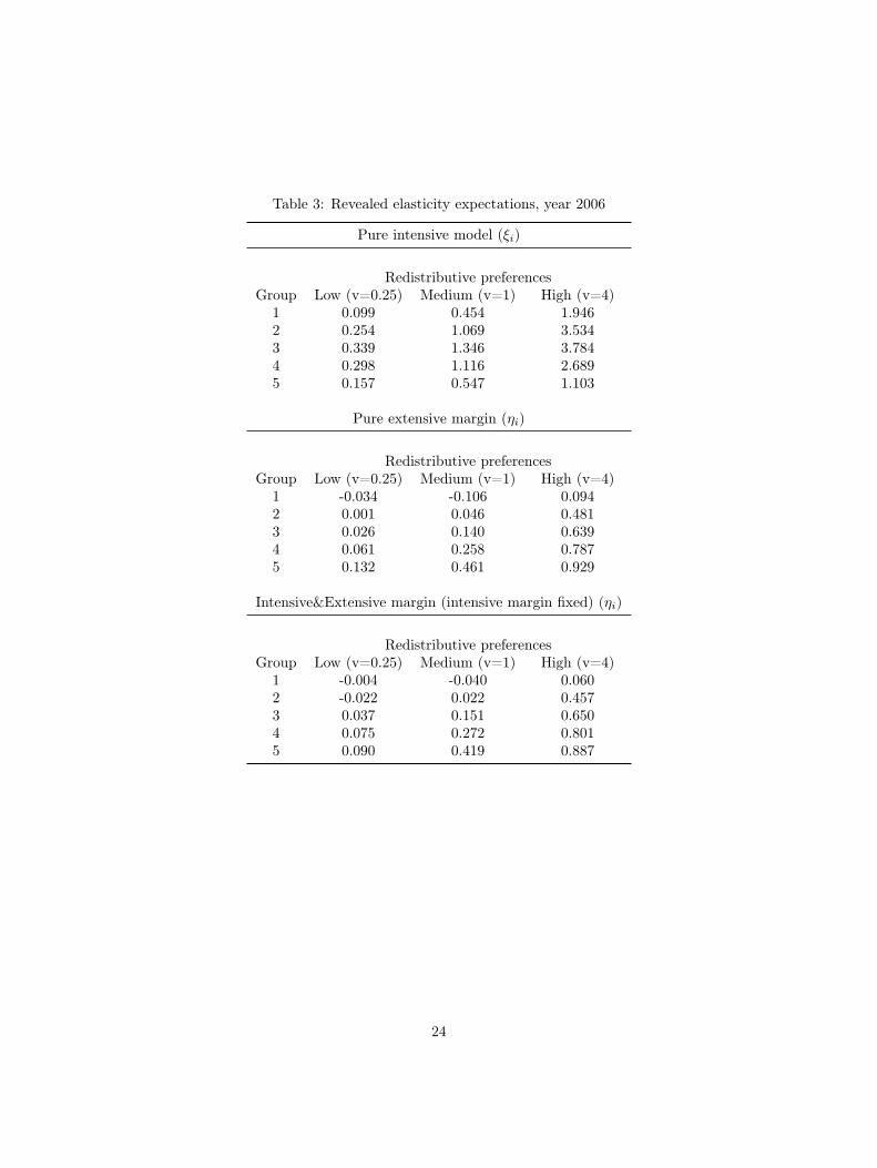
Table 3: Revealed elasticity expectations, year 2006

Pure intensive model (ξi)

Redistributive preferencesGroup Low (v=0.25) Medium (v=1) High (v=4)

1 0.099 0.454 1.9462 0.254 1.069 3.5343 0.339 1.346 3.7844 0.298 1.116 2.6895 0.157 0.547 1.103

Pure extensive margin (ηi)

Redistributive preferencesGroup Low (v=0.25) Medium (v=1) High (v=4)

1 -0.034 -0.106 0.0942 0.001 0.046 0.4813 0.026 0.140 0.6394 0.061 0.258 0.7875 0.132 0.461 0.929

Intensive&Extensive margin (intensive margin fixed) (ηi)

Redistributive preferencesGroup Low (v=0.25) Medium (v=1) High (v=4)

1 -0.004 -0.040 0.0602 -0.022 0.022 0.4573 0.037 0.151 0.6504 0.075 0.272 0.8015 0.090 0.419 0.887

24

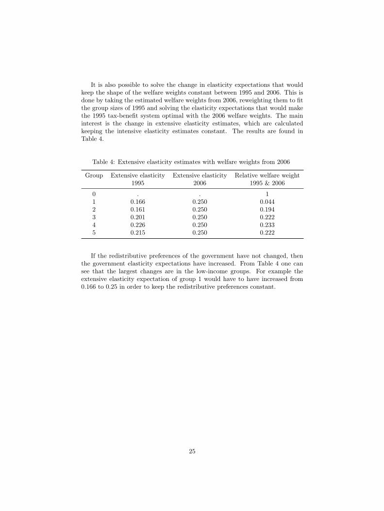
It is also possible to solve the change in elasticity expectations that wouldkeep the shape of the welfare weights constant between 1995 and 2006. This isdone by taking the estimated welfare weights from 2006, reweighting them to fitthe group sizes of 1995 and solving the elasticity expectations that would makethe 1995 tax-benefit system optimal with the 2006 welfare weights. The maininterest is the change in extensive elasticity estimates, which are calculatedkeeping the intensive elasticity estimates constant. The results are found inTable 4.

Table 4: Extensive elasticity estimates with welfare weights from 2006

Group Extensive elasticity Extensive elasticity Relative welfare weight1995 2006 1995 & 2006

0 . . 11 0.166 0.250 0.0442 0.161 0.250 0.1943 0.201 0.250 0.2224 0.226 0.250 0.2335 0.215 0.250 0.222

If the redistributive preferences of the government have not changed, thenthe government elasticity expectations have increased. From Table 4 one cansee that the largest changes are in the low-income groups. For example theextensive elasticity expectation of group 1 would have to have increased from0.166 to 0.25 in order to keep the redistributive preferences constant.

25

6 ConclusionsThe objective of this paper was to analyze the government preferences for re-distribution in Finland by using an inverted optimal income tax model. Bycalculating welfare weights that make the current tax-benefit system optimal itis possible to analyze the redistributive preferences implied by the actual taxsystem. The revealed welfare weights in Finland are not monotonically decreas-ing. The welfare weight of the working poor is much smaller than the rest ofthe welfare weights. The small welfare weight is caused by high participationtax rates combined with significant participation elasticities. The labour supplyelasticity estimates have a large effect on the revealed welfare weights. In apure intensive model with no participation effects the welfare weights are closeto utilitarian preferences.

Several in-work related policy changes were made to the Finnish tax-benefitsystem in the recent decade that might be caused by changes in the socialpreferences behind the tax-benefit system. Therefore the relative welfare weightswere calculated separately for years 1995, 2001 and 2006 in order to see if therevealed welfare weights have changed over time. The welfare weights of allgroups except the unemployed increased such that the largest increase was inthe groups with the least amount of labour income. Therefore the dip in thewelfare weight of the working poor was smaller in 2006 than it was in 1995. Thechange in welfare weights was similar also with a pure intensive model.

The total change in welfare weights was close to the direct change due topolicy reforms that was estimated using a decomposition approach. This indi-cates that the changes in revealed redistributive preferences can be for the mostpart explained by changes in the tax-benefit system.

There are several reasons why the revealed redistributive preferences mighthave changed between 1995 and 2006. One possible reason is that the true socialpreferences for redistribution have changed. The survey results indicate thatthis might be a plausible explanation. The change in the revealed redistributivepreferences of the government could also be due to political changes in thegovernment. However most of the change happened over a time period whenthe government did not change. After the government changed in 2003 thereseems to have been almost no changes in the revealed redistributive preferences.

If the redistributive preferences have not changed, then the elasticity expec-tations of the government have changed so that the decrease in effective taxrates is based on efficiency grounds. The results show that if the redistribu-tive preferences have not changed, the extensive elasticity expectations haveincreased so that the largest changes are in the low-income groups.

For a given set of redistributive preferences, the elasticity expectations ofthe government would have to be large and concentrated on middle- and high-income earners in order for the current tax-benefit system to be optimal.

It should be noted that the analysis covers only direct taxation of labourincome. It is likely that the shape of the tax-benefit system is also affected byother margins, for example the taxation of capital income. If people can shift

26

their income between labour and capital income, then the effective marginaltax rates on labour income might be lower than they would be without incomeshifting.

It can be questioned if the assumption of a welfare maximizing social planneris valid for real tax-benefit systems. Political economy literature addresses theissue that true tax-benefit systems are constructed by political parties who mustwin elections (see e.g. Castanheira et al. 2012). However the welfare maximizingsocial planner can be used as a proxy for more complex political economy models(Coughlin 1992). Still, it would be interesting to extend the inversion methodto political economy models.

There are several potential avenues for future research. One possible exten-sion would be to study the changes in elasticity estimates. The correct valueswould be the government expectations for the elasticities. Unfortunately specificlabour supply elasticity estimates have not been used in Finland when estimat-ing the impacts of tax reforms and the calculations have been done using staticmicrosimulation models only. However in the future when tax reform estima-tions are done using behavioral microsimulations the government expectationsfor elasticities can be found in the calculations.

The decomposition analysis could be extended in order to estimate morethoroughly the composition of the changes in welfare weights using a discretelabour supply model to estimate the expected behavioral effects as in Bargain(2012).

Finally research on the revealed social welfare weights could be extended byallowing the welfare weights to be endogenous. Saez & Stantcheva (2013) pro-pose a generalized optimal taxation theory using a tax reform approach whereendogenous social marginal welfare weights directly reflect society’s views onjustice. Saez & Stantcheva (2013) show how the model can be used to study op-timal family taxation or account for political economy restrictions. Endogenoussocial marginal welfare weights also allow the model to account for horizontalequity concerns.

27

References[1] Ahmad, E., Stern, N. (1984). The theory of reform and Indian direct taxes.

Journal of Public Economics, 25, 259–298.

[2] Bargain, O. (2012). Decomposition analysis of distributive policies us-ing behavioural simulations. International Tax and Public Finance, 19(5),708–731.

[3] Bargain, O., Callan, T. (2010). Analysing the effects of tax-benefit reformson income distribution: a decomposition approach. Journal of EconomicInequality, 8, 1–21

[4] Bargain, O., Dolls, M., Immervoll, H., Neumann, D., Peichl, A., Pestel,N., Siegloch, S., (2013b). Partisan Tax Policy and Income Inequality in theU.S., 1979-2007. IZA Discussion Paper No. 7190.

[5] Bargain, O., Dolls, M., Neumann, D., Peichl, A., Siegloch, S. (2013a). Com-paring Inequality Aversion across Countries When Labor Supply ResponsesDiffer IZA Discussion Paper No. 7215.

[6] Bargain, O., Keane, C. (2010). Tax-Benefit Revealed Redistributive Pref-erences Over Time: Ireland 1987–2005. LABOUR, 24, 141–167.

[7] Bargain, O., Orsini, K. (2006). In-work policies in Europe: Killing twobirds with one stone? Labour Economics, 13, 667–697.

[8] Bourguignon, F., Spadaro, A. (2012). Tax-benefit revealed social prefer-ences. Journal of Economic Inequality, 10(1), 75–108.

[9] Blundell, R., Brewer, M., Haan, P., Shephard, A. (2009). Optimal incometaxation of lone mothers: An empirical comparison of the UK and Germany.The Economic Journal, 119, F101–F121.

[10] Coughlin, P. (1992). Probabilistic Voting Theory. Cambridge: CambridgeUniversity Press.

[11] Castanheira, M., Nicodème, G., Profeta, P. (2012). On the political eco-nomics of tax reforms: survey and empirical assessment. International Taxand Public Finance 19(4). 598–624.

[12] Haan, P., Navarro, D. (2008). Optimal Income Taxation of Married Cou-ples: An Empirical Analysis of Joint and Individual Taxation. IZA Discus-sion Paper No. 3819.

[13] Haan, P., Wrohlich, K. (2010). Optimal Taxation: The Design of ChildRelated Cash- and In-Kind-Benefits. German Economic Review, 11(3),278–301.

28

[14] Immervoll, H., Kleven, H. J., Kreiner, C.T., Verdelin, N. (2011). Opti-mal tax and transfer programs for couples with extensive labor supplyresponses. Journal of Public Economics, 95(11-12), 1485–1500.

[15] Mirrlees, J.A. (1971). An exploration in the theory of optimal income tax-ation. Review of Economic Studies, 38, 175–208.

[16] Pirttilä, J, Uusitalo, R. (2010). A “Leaky Bucket” in the Real World: Es-timating Inequality Aversion using Survey Data. Economica, 77, 60–76.

[17] Saez, E. (2002). Optimal income transfer programs: intensive versus exten-sive labor supply responses. Quarterly Journal of Economics, 117, 1039–73.

[18] Saez, E., Slemrod, J., Giertz, S. (2012). The Elasticity of Taxable Incomewith Respect to Marginal Tax Rates: A Critical Review. Journal of Eco-nomic Literature, 50(1), 3–50.

[19] Saez, E., Stantcheva, S. (2013). Generalized Social Marginal WelfareWeights for Optimal Tax Theory. NBER Working Paper No. 18835

[20] Spadaro, A., Mangiavacchi, L., Piccoli, L. (2012). Optimal taxation, socialcontract and the four worlds of welfare capitalism. Universitat de les IllesBalears DEA Working Paper 52.

29

AppendixRobustness analysis

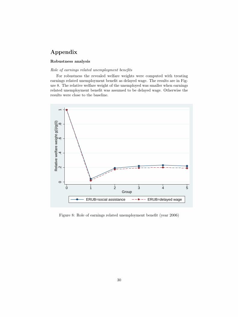
Role of earnings related unemployment benefitsFor robustness the revealed welfare weights were computed with treating

earnings related unemployment benefit as delayed wage. The results are in Fig-ure 8. The relative welfare weight of the unemployed was smaller when earningsrelated unemployment benefit was assumed to be delayed wage. Otherwise theresults were close to the baseline.

0.2

.4.6

.81

Rel

ativ

e w

elfa

re w

eigh

t g(i)

/g(0

)

0 1 2 3 4 5Group

ERUB=social assistance ERUB=delayed wage

Figure 8: Role of earnings related unemployment benefit (year 2006)

30

Alternative cutoff points for income groupsIn the baseline calculations income groups were constructed using income

quintiles in different years. Therefore the cutoff points were different each yearpartly due to changes in the income distribution. In the robustness check thecutoff points of 1995 income quintiles are used. The cutoff points were upratedusing average wage growth between 1995 and 2006. The results are in Figure 9.The welfare weights seem to be robust to the choice of cutoff points.

0.2

.4.6

.81

Rel

ativ

e w

elfa

re w

eigh

t g(i)

/g(0

)

0 1 2 3 4 5Group

Groups: 2006 quintiles Groups: 1995 quintiles (uprated)

Figure 9: Different cutoff points for income groups (year 2006)

31

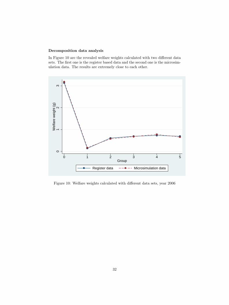
Decomposition data analysis

In Figure 10 are the revealed welfare weights calculated with two different datasets. The first one is the register based data and the second one is the microsim-ulation data. The results are extremely close to each other.

01

23

Wel

fare

wei

ght (

g)

0 1 2 3 4 5Group

Register data Microsimulation data

Figure 10: Welfare weights calculated with different data sets, year 2006

32