Revealing Asymmetries in the HD 181327 Debris Disk: A Recent

Massive Collision or ISM Warping

Christopher C. Stark1, Glenn Schneider2, Alycia J. Weinberger3, John H. Debes4, Carol A.

Grady5, Hannah Jang-Condell6, Marc J. Kuchner7

ABSTRACT

New multi-roll coronagraphic images of the HD 181327 debris disk obtained

using the Space Telescope Imaging Spectrograph (STIS) on board the Hubble

Space Telescope (HST) reveal the debris ring in its entirety at high SNR and

unprecedented spatial resolution. We present and apply a new multi-roll image

processing routine to identify and further remove quasi-static PSF-subtraction

residuals and quantify systematic uncertainties. We also use a new iterative im-

age deprojection technique to constrain the true disk geometry and aggressively

remove any surface brightness asymmetries that can be explained without invok-

ing dust density enhancements/deficits. The measured empirical scattering phase

function for the disk appears more forward scattering than previously thought

and is not well-fit by a Henyey-Greenstein function. The empirical scattering

phase function varies with stellocentric distance, consistent with the expected

radiation pressured-induced size segregation exterior to the belt, but in contra-

diction to unperturbed debris ring models within the belt, suggesting the presence

of an unseen planet exterior to the belt. We detect large scale asymmetries in

the disk, consistent with either the recent catastrophic disruption of a body with

mass > 1% the mass of Pluto, or disk warping due to strong ISM interactions.

1NASA Goddard Space Flight Center, Exoplanets & Stellar Astrophysics Laboratory, Code 667, Green-

belt, MD 20771; christopher.c.stark@nasa.gov

2Steward Observatory, The University of Arizona, Tucson, AZ 85721

3Department of Terrestrial Magnetism, Carnegie Institution of Washington, 5241 Broad Branch Road

NW, Washington, DC 20015

4Space Telescope Science Institute, Baltimore, MD 21218

5Eureka Scienti?c, 2452 Delmer, Suite 100, Oakland, CA 96002

6Department of Physics & Astronomy, University of Wyoming, Laramie, WY 82071

7NASA Goddard Space Flight Center, Exoplanets & Stellar Astrophysics Laboratory, Code 667, Green-

belt, MD 20771

– 2 –

Subject headings: circumstellar matter — planet–disk interactions — methods:

observational — stars : individual (HD 181327)

1. Introduction

Images of spatially resolved debris disks show a range of spectacular asymmetries in-

cluding eccentric rings (e.g. Kalas et al. 2005; Schneider et al. 2009; Krist et al. 2012; Boley

et al. 2012), warps and sub-substructures (e.g. Golimowski et al. 2006; Krist et al. 2005),

and various other morphologies (e.g. Hines et al. 2007; Kalas et al. 2007). Interpreting sur-

face brightness asymmetries as dust density variations and explaining them via dynamic

processes has been popular since coronagraphic images of the Beta Pictoris disk revealed

several different kinds of asymmetries in the starlight scattered at optical and near-IR wave-

lengths (Kalas & Jewitt 1995). Recently, ALMA has begun to explore such patterns at

unprecedented resolution at submillimter wavelengths (e.g. Boley et al. 2012).

Many models have shown that exoplanets can create asymmetric dust distributions in

debris disks via gravitational perturbations–a tantalizing prospect since this process can

reveal the presence of otherwise undetected planets and constrain their orbital parameters.

This process could be the only way to detect true Neptune analogs orbiting nearby stars on

reasonable timescales. Direct images of exoplanet candidates associated with debris disks

have begun to demonstrate both the potential and complexities of this concept for locating

new planets and constraining their properties (e.g. Quillen 2006; Chiang et al. 2009; Lagrange

et al. 2010; Kalas et al. 2013)

Many other dynamical processes can also produce dust density asymmetries in debris

disks. Disks can interact with the interstellar medium (Artymowicz & Clampin 1997; Debes

et al. 2009; Maness et al. 2009; Marzari & Thebault 2011). In the solar system, collisions of

asteroids can produce detectable trails of debris (Jewitt et al. 2010); in debris disks, recent

collisions can potentially yield detectable arcs of debris (Grigorieva et al. 2007; Kral et al.

2013).

However, it remains crucial to pursue explanations for debris disk asymmetries other

than density enhancements/deficits. The observed scattered starlight from a disk is a com-

plex combination of the disk’s geometry, illumination, and stellocentric grain-size segregation,

the dust grains’ size-dependent scattering efficiency and scattering phase function, and line-

of-sight projection effects in the case of inclined disks (e.g. ansal brightening for disks with

large scale heights). All of these effects are degenerate to some degree and, given our current

– 3 –

understanding of dust grain scattering properties, are exceedingly difficult to disentangle.

In light of this, we interpret new multi-roll STIS coronagraphic images of the HD 181327

debris disk by aggressively pursuing explanations for observed asymmetries other than den-

sity enhancements. We exploit a symmetry in the scattering phase function to search for

deviations from a smooth disk.

HD 181327 is an F5/6, ∼ 12 Myr old main sequence member of the β Pic moving group,

located at a distance of 51.8 pc (Schneider et al. 2006). HD 181327 has a strong thermal IR

excess (LIR/L? = 0.25%) attributed to re-radiating circumstellar dust. This debris disk was

first detected with IRAS (Mannings & Barlow 1998) and subsequently resolved at 0.6 µm

with the Advanced Camera for Surveys (ACS), 1.1 µm with the Near Infrared Camera and

Multi-Object Spectrometer (NICMOS) on HST (Schneider et al. 2006), 18.3 µm with Gemini

South T-ReCS (Chen et al. 2008), and 3.2 mm with the Australian Telescope Compact Array

(ATCA) (Lebreton et al. 2012). All resolved observations are consistent with a ring of dust

with radius ∼ 90 AU and a cleared interior. Most resolved images suggest clumpy asymme-

tries, but also have low SNR, so we refrain from incorporating those previous observations

into our analysis.

In Section 2 we briefly describe our new STIS observations of HD 181327 and present a

new PSF residual removal routine. For a more detailed description of the observations, see

Schneider (2014, in prep.). In Section 3, we detail our image deprojection techniques and

ascertain the minimally-asymmetric face-on optical depth. In Section 4, we interpret the

observed scattering phase function and present evidence for a recent massive collision.

2. Observations & Data Reduction

As part of the HST GO 12228 (PI: G. Schneider) observation program, we observed

HD 181327 with the HST STIS coronagraph at 6 roll angles, each at 2 wedge-occulter

positions (WedgeA0.6 and WedgeA1.0, which have occulting half-widths of 0.4′′and 0.5′′,

respectively1). Each observational configuration (a given roll angle and wedge position) has

multiple exposure images that we median-combined into a single image prior to template

PSF subtraction. We then rotated the PSF-subtracted image for each observational con-

figuration to the celestial orientation and median combined all images into a single high

contrast image. Our multi-roll observation method reduces the mean inner working angle

of the STIS coronagraph, reduces the influence of PSF artifacts, and improves SNR. We

1See the HST STIS instrument handbook for a full description.

– 4 –

observed HD 181327 over 3 orbits on 20 May, 2011 and 3 orbits on 10 July, 2011, and the

(B − V color-matched) PSF reference star HD 180134 at each wedge position and a single

roll angle interleaved with the target observations. Table 1 summarizes the observations.

All astrometric measurements of the HD 181327 debris ring are referenced to the position

of the coronagraphically occulted star, as measured individually from twelve independent

images using the diffraction spikes in each image to locate the star. In each of the twelve

images, the uncertainty in the target position is approximately 0.3 pixels (0.8 AU) in the

Science Aperture Instrument (detector) Frame (SIAF) x and y directions. In the twelve-

image combination, the uncertainty is reduced to ±0.087 pixels, or ±4.4 mas (0.23 AU); this

is comparable to the HST pointing stability (RMS 2-guide star fine-lock jitter). The mean

stellar position is used to anchor the inter- and intra-visit stellar location following target

acquisition slews and to reference the WedgeA0.6 pointings to the WedgeA1.0 pointings.

All PSF subtractions are done in the SIAF frame, aligned by subtraction spike residual

minimization. Each image is then rotated about the mean stellar position to a common

north-up orientation. We then manually build a mask specific to each observation, flagging

those pixels that are obscured by the occulting wedge, corrupted by diffraction spikes, satu-

rated or adversely affected by wedge-edge artifacts, or are beyond the FOV sub-array read

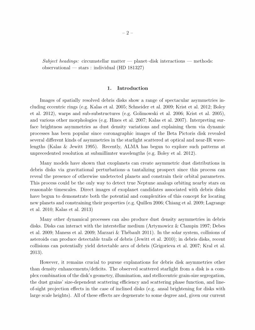
out. Finally, we median-combine the 12 astrometrically co-registered images in the common

celestial frame. Figure 1 shows the inner 200 × 200 pixels (pixel scale = 50.77 mas, or 2.63

AU assuming a distance of 51.8 pc) of our 12-image median alongside a map of the number

of observations per pixel, npix.

– 5 –

Table 1. Observations

Target Orientation Exposures Total Exposure Time Wedge Date

() (s)

HD 181327 222.738 8 175.2 0.6A 20 May 2011

222.738 8 175.2 0.6A 20 May 2011

222.738 4 87.6 0.6A 20 May 2011

222.738 4 1708.0 1.0A 20 May 2011

242.738 8 175.2 0.6A 20 May 2011

242.738 8 175.2 0.6A 20 May 2011

242.738 4 87.6 0.6A 20 May 2011

242.738 4 1708.0 1.0A 20 May 2011

HD 180134 243.219 8 95.2 0.6A 20 May 2011

243.219 8 95.2 0.6A 20 May 2011

243.219 8 95.2 0.6A 20 May 2011

243.219 8 1656.0 1.0A 20 May 2011

HD 181327 262.738 8 175.2 0.6A 20 May 2011

262.738 8 175.2 0.6A 20 May 2011

262.738 4 87.6 0.6A 20 May 2011

262.738 4 1708.0 1.0A 20 May 2011

293.056 8 175.2 0.6A 10 July 2011

293.056 8 175.2 0.6A 10 July 2011

293.056 4 87.6 0.6A 10 July 2011

293.056 4 1644.0 1.0A 10 July 2011

313.556 8 175.2 0.6A 10 July 2011

313.556 8 175.2 0.6A 10 July 2011

313.556 4 87.6 0.6A 10 July 2011

313.556 4 1708.0 1.0A 10 July 2011

HD 180134 314.232 8 95.2 0.6A 10 July 2011

314.232 8 95.2 0.6A 10 July 2011

314.232 8 95.2 0.6A 10 July 2011

314.232 8 1656.0 1.0A 10 July 2011

HD 181327 334.056 8 175.2 0.6A 10 July 2011

334.056 8 175.2 0.6A 10 July 2011

334.056 4 87.6 0.6A 10 July 2011

334.056 4 1708.0 1.0A 10 July 2011

– 6 –

N

E1"

0.00 2.00 3.99 5.99Flux density (counts second−1 pixel−1)

0.00 2.00 3.99 5.99Flux density (counts second−1 pixel−1)

0 4 8 12Number of observations

0 4 8 12Number of observations

Fig. 1.— Left: Central 200×200 pixels of the 12-image median-combined image for HD

181327 (pixel scale = 50.77 mas = 2.63 AU). An artificial occulting spot with a radius of

18 pixels has been applied for illustrative purposes. Stellar position is marked with a star.

Right: Number of images used per pixel for median combination.

Our multi-roll observation technique reduces both the impact of temporal instabilities

in the PSF structures (“breathing”) and static PSF residuals that co-rotate with the in-

strument/telescope optics. To estimate the remaining impact of PSF artifacts, we produced

an 11-image median, subtracted it from the 12-image median, and divided by the 12-image

median to produce a fractional residual map. If the 12-image median is robust to these

PSF residuals, then leaving out any one image should not greatly impact the final image.

Figure 2 shows one such fractional residual map. The fractional residuals, smoothed using a

3×3 pixel median boxcar and displayed on a saturated scale for illustrative purposes, show

correlated biases in the median by as much as ∼ 5% over scales ∼ 10 pixels. Additionally,

Figure 2 shows that leaving out this particular image affects the NE-SW asymmetry at this

level by enhancing the NE flux and reducing the SW flux.

– 7 –

< −5 −2.5 0 2.5 > 5

Difference (%)

< −5 −2.5 0 2.5 > 5

Difference (%)

Fig. 2.— Relative difference between a representative 11-image median and the 12-image

median (central 200×200 pixels). PSF residuals in a single image can bias the flux of the

12-image median by ∼ 5% over scales ∼ 10 pixels or larger.

Although we cannot remove the time-dependent PSF residuals with this method, we

can better mitigate the static PSF residuals. We did this using the following “multi-roll

residual removal routine” (MRRR, pronounced “myrrh”):

1. Form the 12-image median, oriented north-up.

2. Subtract the 12-image median from each individual masked image, oriented north-up,

to form 12 disk-less residual images.

3. De-rotate each disk-less residual image to the SIAF-oriented frame.

4. Take the median of the 12 disk-less residual images to produce a map of static residuals.

– 8 –

5. Smooth the static residual map using a 3×3 median boxcar to remove pixel-to-pixel

noise, retaining only larger scale correlated residuals.

6. Subtract the smoothed, correlated residual map from each of the 12 images in the SIAF

frame, rotate each to the north-up frame, and form a new residual-removed 12 image

median.

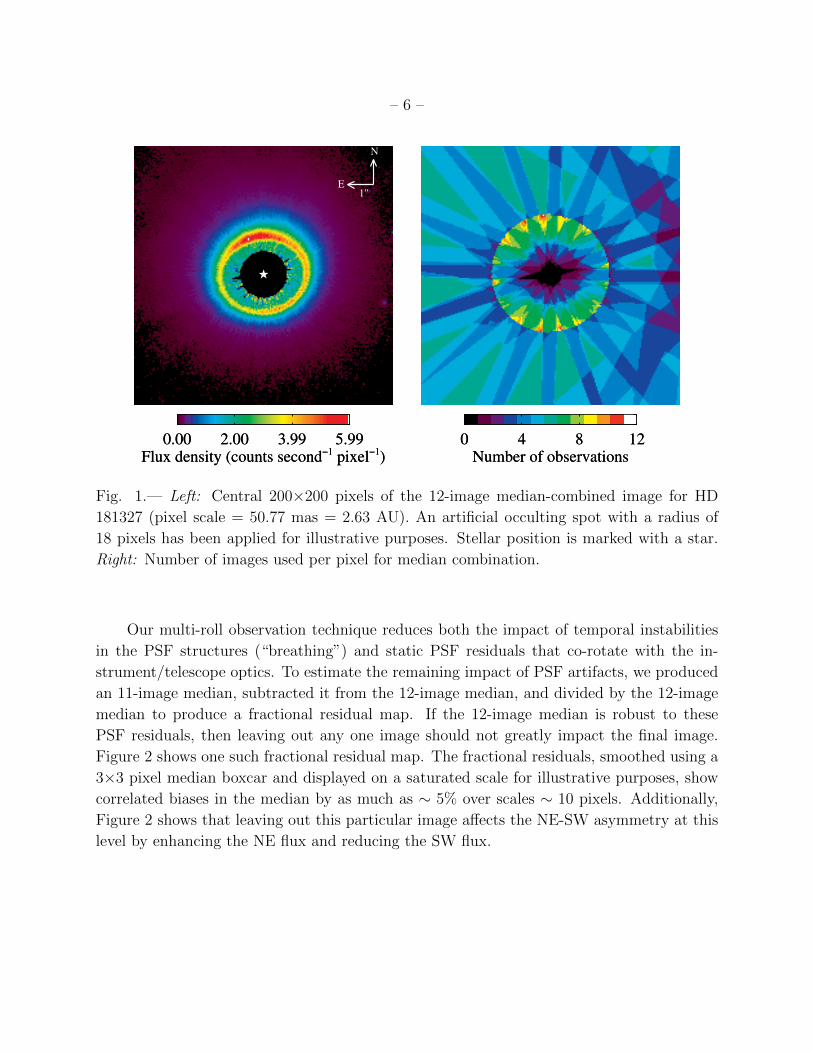
Figure 3 shows the smoothed, correlated residual map for the inner 200×200 pixels of our

observations of the HD 181327 disk (displayed on a saturated scale for illustration). Figure 4

shows the final residual-removed 12 image median, and the fractional difference between the

original 12-image median and the residual-removed 12 image median. In this case, MRRR

dims the ansae by ∼ 5% and brightens the SW side of the ring by ∼ 5%. Not surprisingly,

the regions of the disk impacted most significantly are the regions with small values of npix

(see Figure 1). We use the MRRR-corrected image for all subsequent analysis in this work.

– 9 –

< −10 −5 0 5 > 10

Relative flux (%)

< −10 −5 0 5 > 10

Relative flux (%)

Fig. 3.— Static PSF residuals common to all images in SIAF frame, smoothed by a 3×3

boxcar median (central 200×200 pixels). We remove these residuals from each individual

image to create an improved multi-roll median image.

– 10 –

N

E1"

0.00 1.48 2.96 4.45 5.93Flux density (counts second−1 pixel−1)

0.00 1.48 2.96 4.45 5.93Flux density (counts second−1 pixel−1)

−10.0 −3.3 3.3 10.0Percent Difference (%)

−10.0 −3.3 3.3 10.0Percent Difference (%)

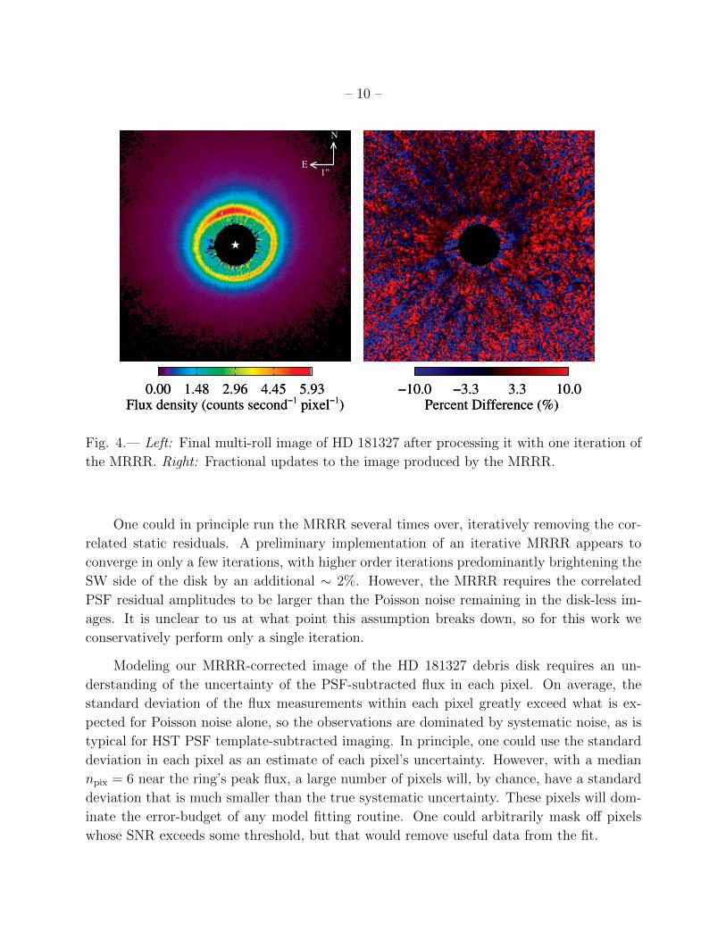
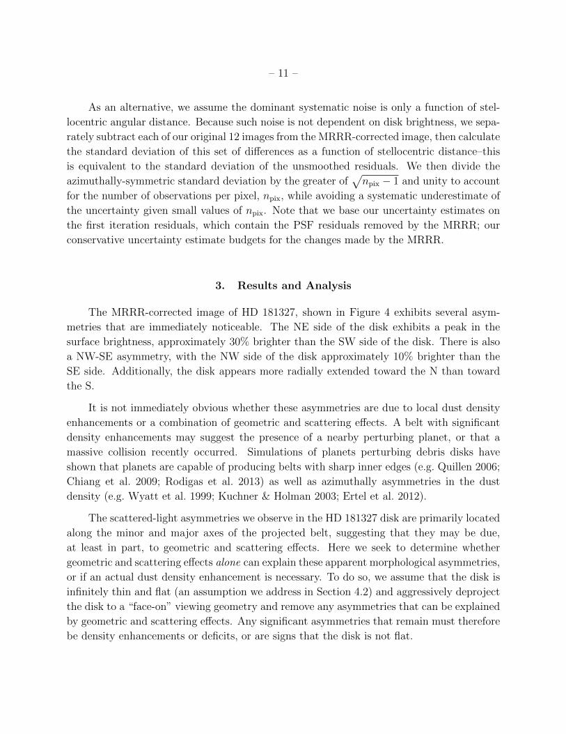
Fig. 4.— Left: Final multi-roll image of HD 181327 after processing it with one iteration of

the MRRR. Right: Fractional updates to the image produced by the MRRR.

One could in principle run the MRRR several times over, iteratively removing the cor-

related static residuals. A preliminary implementation of an iterative MRRR appears to

converge in only a few iterations, with higher order iterations predominantly brightening the

SW side of the disk by an additional ∼ 2%. However, the MRRR requires the correlated

PSF residual amplitudes to be larger than the Poisson noise remaining in the disk-less im-

ages. It is unclear to us at what point this assumption breaks down, so for this work we

conservatively perform only a single iteration.

Modeling our MRRR-corrected image of the HD 181327 debris disk requires an un-

derstanding of the uncertainty of the PSF-subtracted flux in each pixel. On average, the

standard deviation of the flux measurements within each pixel greatly exceed what is ex-

pected for Poisson noise alone, so the observations are dominated by systematic noise, as is

typical for HST PSF template-subtracted imaging. In principle, one could use the standard

deviation in each pixel as an estimate of each pixel’s uncertainty. However, with a median

npix = 6 near the ring’s peak flux, a large number of pixels will, by chance, have a standard

deviation that is much smaller than the true systematic uncertainty. These pixels will dom-

inate the error-budget of any model fitting routine. One could arbitrarily mask off pixels

whose SNR exceeds some threshold, but that would remove useful data from the fit.

– 11 –

As an alternative, we assume the dominant systematic noise is only a function of stel-

locentric angular distance. Because such noise is not dependent on disk brightness, we sepa-

rately subtract each of our original 12 images from the MRRR-corrected image, then calculate

the standard deviation of this set of differences as a function of stellocentric distance–this

is equivalent to the standard deviation of the unsmoothed residuals. We then divide the

azimuthally-symmetric standard deviation by the greater of√npix − 1 and unity to account

for the number of observations per pixel, npix, while avoiding a systematic underestimate of

the uncertainty given small values of npix. Note that we base our uncertainty estimates on

the first iteration residuals, which contain the PSF residuals removed by the MRRR; our

conservative uncertainty estimate budgets for the changes made by the MRRR.

3. Results and Analysis

The MRRR-corrected image of HD 181327, shown in Figure 4 exhibits several asym-

metries that are immediately noticeable. The NE side of the disk exhibits a peak in the

surface brightness, approximately 30% brighter than the SW side of the disk. There is also

a NW-SE asymmetry, with the NW side of the disk approximately 10% brighter than the

SE side. Additionally, the disk appears more radially extended toward the N than toward

the S.

It is not immediately obvious whether these asymmetries are due to local dust density

enhancements or a combination of geometric and scattering effects. A belt with significant

density enhancements may suggest the presence of a nearby perturbing planet, or that a

massive collision recently occurred. Simulations of planets perturbing debris disks have

shown that planets are capable of producing belts with sharp inner edges (e.g. Quillen 2006;

Chiang et al. 2009; Rodigas et al. 2013) as well as azimuthally asymmetries in the dust

density (e.g. Wyatt et al. 1999; Kuchner & Holman 2003; Ertel et al. 2012).

The scattered-light asymmetries we observe in the HD 181327 disk are primarily located

along the minor and major axes of the projected belt, suggesting that they may be due,

at least in part, to geometric and scattering effects. Here we seek to determine whether

geometric and scattering effects alone can explain these apparent morphological asymmetries,

or if an actual dust density enhancement is necessary. To do so, we assume that the disk is

infinitely thin and flat (an assumption we address in Section 4.2) and aggressively deproject

the disk to a “face-on” viewing geometry and remove any asymmetries that can be explained

by geometric and scattering effects. Any significant asymmetries that remain must therefore

be density enhancements or deficits, or are signs that the disk is not flat.

– 12 –

To deproject the observations and examine the face-on optical depth of the disk we

employed the following process:

1. Fit the observed (projected) HD 181327 dust belt with an ellipse

2. Deproject the ellipse to obtain the true orbital ellipse and disk geometry

3. Using the true orbital ellipse values in the projected image plane, correct for the 1/r2

illumination factor

4. Determine the best fit scattering phase function and divide it out of the image

5. Deproject the image to produce a final face-on optical depth image

6. Examine the optical depth for remaining density asymmetries

Below we discuss this process step by step. In practice, steps 1 – 3 were incorporated into

their own iterative subroutine which we describe below. We will repeatedly refer to Figure

6, which illustrates each step of this process.

3.1. Projected ellipse fitting

There are many ways to fit an ellipse to the HD 181327 dust ring shown in Figure

4. First, we must choose a metric that defines the ellipse, e.g. the location of the belt’s

peak flux, an isophote, the belt’s inner edge, etc. It is unclear which metric of the disk

ring structure is most useful to define our ellipse. Ideally we’d choose a metric that reflects

the underlying density distribution, e.g. the peak density of the belt. However, the radial

location of the peak surface brightness does not correspond to the radial location of the peak

density, because the differential 1/r2 illumination factor shifts the apparent peak location

(an especially important factor for eccentric debris rings). We must correct for the 1/r2

illumination factor to fit the orientation of the disk, but we must know the orientation of

the disk to correct for the 1/r2 illumination factor.

In light of this catch-22, we developed a method to fit the illumination-corrected image

by iterating steps 1 – 3 of our disk deprojection procedure. First, we guessed the orientation

of the disk (e.g. circular and face-on). We then generated a map of 1/r2 and used it

to remove the stellar illumination. We then recorded the coordinates of the illumination-

corrected projected belt maximum, fit these coordinates with an ellipse, and deprojected the

ellipse to obtain a new disk orientation. We iterated this process, using updated 1/r2 maps

– 13 –

each time. It’s unclear whether this procedure should converge in all cases, but in the case

of HD 181327, we found that this process converged in ∼ 3 iterations regardless of our initial

guess of the disk orientation.

We used polar coordinates to measure the projected radius of the peak illumination-

corrected surface brightness, which we refer to loosely as the surface density. We calculated

on-sky ρ and φ values for each pixel’s center relative to the star location. We divided the

surface density image into 172 wedges with angular size of 2.1 centered on the star, chosen

such that the arc length of a wedge is ∼ 1 pixel at the location of the projected belt’s semi-

minor axis. For each wedge, we plotted the surface density as a function of ρ. We then

selected the 7 pixels with ρ nearest in location to the radius of the peak surface density and

fit the points with a Gaussian to to measure the sub-pixel location of the ring maximum for

that wedge. We repeated this fit while increasing the number of points to 17, using each

pixel’s uncertainty and a Monte Carlo routine to estimate the uncertainty in the locations of

the fit maxima. Finally, we chose the fit with the most certain peak location to estimate the

radial location of the wedge’s peak surface density, ρpeak, and used the average value of φ as

the angular location of the peak, φpeak. This method produces a set of (ρpeak, φpeak) values

marking the belt maximum while minimizing the radial uncertainty.

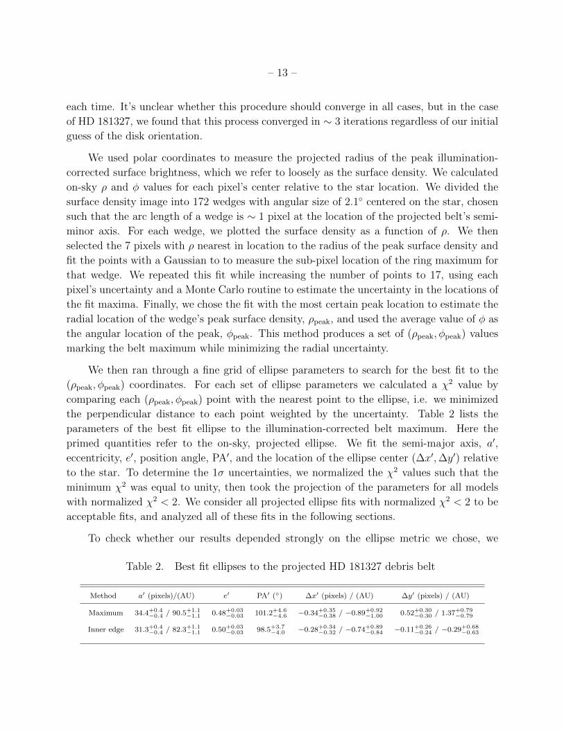
We then ran through a fine grid of ellipse parameters to search for the best fit to the

(ρpeak, φpeak) coordinates. For each set of ellipse parameters we calculated a χ2 value by

comparing each (ρpeak, φpeak) point with the nearest point to the ellipse, i.e. we minimized

the perpendicular distance to each point weighted by the uncertainty. Table 2 lists the

parameters of the best fit ellipse to the illumination-corrected belt maximum. Here the

primed quantities refer to the on-sky, projected ellipse. We fit the semi-major axis, a′,

eccentricity, e′, position angle, PA′, and the location of the ellipse center (∆x′,∆y′) relative

to the star. To determine the 1σ uncertainties, we normalized the χ2 values such that the

minimum χ2 was equal to unity, then took the projection of the parameters for all models

with normalized χ2 < 2. We consider all projected ellipse fits with normalized χ2 < 2 to be

acceptable fits, and analyzed all of these fits in the following sections.

To check whether our results depended strongly on the ellipse metric we chose, we

Table 2. Best fit ellipses to the projected HD 181327 debris belt

Method a′ (pixels)/(AU) e′ PA′ () ∆x′ (pixels) / (AU) ∆y′ (pixels) / (AU)

Maximum 34.4+0.4−0.4 / 90.5+1.1

−1.1 0.48+0.03−0.03 101.2+4.6

−4.6 −0.34+0.35−0.38 / −0.89+0.92

−1.00 0.52+0.30−0.30 / 1.37+0.79

−0.79

Inner edge 31.3+0.4−0.4 / 82.3+1.1

−1.1 0.50+0.03−0.03 98.5+3.7

−4.0 −0.28+0.34−0.32 / −0.74+0.89

−0.84 −0.11+0.26−0.24 / −0.29+0.68

−0.63

– 14 –

repeated this procedure by fitting the inner edge of the belt. To fit the inner edge, we first

calculated the radial derivative of the illumination-corrected HD 181327 image in the true

disk plane, for which the maximum marks the belt’s inner edge. We then fit the maximum

of the radial derivative using the techniques described above. Table 2 lists the results of fits

to the inner edge of the belt. With exception to the values of a′, which should not agree,

and ∆y′, the fits agree to within 1σ, suggesting that in the region of the parent belt, the

disk is thin and flat. The small discrepancy in the ∆y′ values may be a result of the blurring

of radial features along the disk minor axis due to a non-zero disk scale height, which we

address in Section 4.2.

3.2. Ellipse deprojection

To deproject the ellipse fits, i.e. obtain the true elliptical geometry and orientation

of the disk, we used the Kowalsky method, as described by Smart (1930). This analytic

method transforms the parameters describing an apparent ellipse with a center offset from

the star (a′, e′, PA′, ∆x′, ∆y′) into a set of unique, deprojected ellipse parameters (a, e, ω,

i, Ω) describing both the geometry and orientation of the true ellipse. Here a is the true

semi-major axis, e is the true eccentricity, ω is the argument of pericenter, which defines the

axis of inclination in the plane of the disk, i is the inclination, and Ω is the longitude of the

ascending node, which defines the angle of the axis of inclination on the sky.

We applied this method to all of the ellipse fits within 1 σ of the best fit values listed in

Table 2. Table 3 lists the resulting deprojected values. We constrain the disk inclination to

28.5±2, consistent with previous estimates (Schneider et al. 2006), and marginally constrain

the eccentricity to a non-zero value of 0.02 ± 0.01. This small true eccentricity results in

poorly constrained ω. As a result, the pericenter of the HD 181327 disk could be located

anywhere in the SW quadrant of Figure 4.

The red ellipse in Figure 5 shows the best fit to the HD 181327 illumination-corrected

belt maximum. The red line illustrates the major axis of the projected ellipse and the yellow

Table 3. Deprojected ellipse parameters for the HD 181327 debris belt

Method a (AU) e ω () i () Ω ()

Maximum 90.5+1.1−1.1 0.02+0.01

−0.01 −70+32−33 28.5+2.1

−2.0 11.2+4.6−4.6

Inner edge 82.3+1.1−1.1 0.01+0.01

−0.01 16+164−196 30.3+1.9

−2.0 8.5+3.7−4.0

– 15 –

line marks the true major axis with periastron marked with a “p.” The line of nodes (the

axis of inclination of the disk) is nearly coincident with the projected major axis, as expected

for a nearly-circular ring; the line connecting forward to back scattering is approximately

perpendicular to the projected major axis. The center of the ellipse and the star are marked

with a red dot and a yellow star, respectively.

p

N

E1"

Fig. 5.— Best fit ellipse to the belt maximum. The projected major axis and true major axis

are shown in red and yellow, respectively, with periastron at point “p.” The stellar location

is marked with a yellow star.

Table 3 also lists the deprojected ellipse parameters for fits to the inner edge of the belt.

In the case of an infinitely thin uniform disk, we expect the ellipse parameters derived from

fits to the belt maximum and the belt inner edge to agree within their mutual uncertainties,

except for a. A discrepancy between the ellipse geometry of the inner edge and the belt

maximum would suggest that the radial distribution of dust varies significantly, that the

disk is not flat, or that the disk has an opening angle of more than a few degrees. As shown

in Table 3, fits to the illumination-corrected belt maximum and the illumination-corrected

inner edge give consistent values for all parameters and have similar uncertainties; a flat,

– 16 –

thin disk appears to be a reasonable approximation for the HD 181327 debris belt.

3.3. Illumination correction

We next corrected for the 1/r2 stellar illumination factor. We distributed 107 particles

uniformly in azimuth and logarithmically in r from 50 to 800 AU. Using the deprojected

ellipse parameters from the first line of Table 3, we then rotated the 3-D positions by ω,

i, and Ω, and binned the particles into pixels based on their on-sky (x,y) coordinates, the

pixel scale of 50.77 mas, and a distance to HD 181327 of 51.8 pc. Finally, we calculated

the average 1/r2 value in each pixel to produce a 〈1/r2〉 map, which we divided into the HD

181327 STIS image.

Figure 6 shows this portion of the deprojection process. Panel (a) shows the initial HD

181327 STIS image. Panel (b) shows the 〈1/r2〉 map for the deprojected ellipse fit listed in

the first line of Table 3, normalized to the radial peak of the birth ring at 90.5 AU. Panel

(c) shows the illumination-corrected image, given by the HD 181327 STIS image divided by

the 〈1/r2〉 map.

– 17 –

N

E1"

N

E

N

E

0.00 1.98 3.95 5.93Flux density (counts s−1 pixel−1)

0.00 1.98 3.95 5.93Flux density (counts s−1 pixel−1)

0.00 0.81 1.62 2.44(90.5 AU)2/r2

0.00 0.81 1.62 2.44(90.5 AU)2/r2

0.00 1.98 3.96 5.95Illumination−corrected flux dens. (counts s−1 pix−1)

0.00 1.98 3.96 5.95Illumination−corrected flux dens. (counts s−1 pix−1)

61 80 100 119Average scattering angle (o)

61 80 100 119Average scattering angle (o)

58 177 296 415Average semi−major axis (AU)

58 177 296 415Average semi−major axis (AU)

0.62 1.27 1.92 2.57Scattering phase function

0.62 1.27 1.92 2.57Scattering phase function

0.00 0.33 0.67 1.00Normalized optical depth

0.00 0.33 0.67 1.00Normalized optical depth

0.00 0.33 0.67 1.00Normalized optical depth

0.00 0.33 0.67 1.00Normalized optical depth

a b c d

e f g h

Fig. 6.— Deprojection procedure. a) Original STIS image. b) 〈1/r2〉 map normalized to the

birth ring distance of 90.5 AU. c) (a) divided by (b). d) Map of the average scattering angle.

e) Map of the average semi-major axis. f) Best fit scattering phase function map. g) (c)

divided by (f). g) (h) Deprojected optical depth with the belt’s pericenter located directly

to the right of the star. The stellar location is marked in each image with a white star.

3.4. The scattering phase function(s) and density distribution

The scattering phase functions (SPFs) of disks are commonly approximated using a

Henyey-Greenstein (HG)SPF, given by

p (θ) =1

4π

1− g2

[ 1 + g2 − 2g cos θ ]3/2, (1)

where θ is the scattering phase angle and g is the HG asymmetry parameter, ranging from -1

for perfect backscattering to 1 for perfect forward scattering. Small dust grains are known to

be forward scattering, so typically g > 0 for debris disks. However, this function is typically

used out of expedience, not fidelity. SPFs predicted by Mie theory do not resemble HG

functions in many cases, and HG SPF fits to observed debris disks produce g values much

less than is expected for micron sized grains (e.g. Kalas et al. 2005; Schneider et al. 2006;

Debes et al. 2008; Thalmann et al. 2011). Additionally, the SPF of the zodiacal dust cloud

– 18 –

is significantly flatter near a scattering phase angle of 90 than predicted by a single forward

scattering HG phase function (Hong 1985).

Here, we do not limit ourselves to analytic scattering phase functions. Instead, we

fit an empirical scattering phase function to the data. At a given semi-major axis a, the

illumination-corrected flux, F ′, shown in Figure 6c is proportional to

F ′(a, θ) ∝∫

dN(a, θ)

dss2Qsca(s) p(θ, s) ds, (2)

where dN(a, θ)/ds is the differential number of grains of size s, Qsca(s) is the scattering

efficiency, and p(θ, s) is the scattering phase function. In the case of a uniform disk with small

eccentricity, the size distribution is constant along a given semi-major axis, i.e. independent

of θ. As a result, the scattering phase function averaged over grain size

p (a, θ) =

∫ dN(a)ds

s2Qsca(s) p(θ, s) ds∫ dN(a)ds

s2Qsca(s) ds(3)

is a function of a and θ. Therefore we can determine an empirical SPF by fitting the

illumination-corrected flux as a function of a and θ.

Following the same procedure described above for the 〈1/r2〉 map, we created projected

maps of the average scattering phase angle 〈θ〉 (Figure 6d) and the average semi-major axis

〈a〉 (Figure 6e). For a given value of a, we then selected those pixels with |〈a〉 − a| < 2.63

AU (1 pixel width) and fit the illumination-corrected flux as a function of 〈θ〉.

Figure 7 shows the illumination-corrected flux as a function of 〈θ〉 for two values of a.

Here we used the line joining the minimum and maximum scattering phase angles in Figure

6 to divide the disk into a SE half (shown in red) and a NW half (shown in black). In the

case of a uniform disk, the SE and NW scattering phase functions should be identical and

this is approximately true at a = 105 AU, as shown in the top panel of Figure 7. However,

the bottom panel of Figure 7 shows that near the belt maxium, a = 89.4 AU, the two halves

are asymmetric. Under the assumption of a flat, thin disk, such asymmetries cannot be

explained by additional projection or scattering effects and form the foundation by which we

identify density asymmetries.

We fit the flux measurements as a function of scattering phase angle with a fourth degree

polynomial, shown in yellow in Figure 7, to obtain an empirical scattering phase function.

This function could be fit to the flux from the SE half of the disk, the NW half of the disk,

or both halves simultaneously. In the case of HD 181327 the SE disk flux is consistently less

than the NW flux. We chose to interpret any detected asymmetries as density enhancements,

so we fit the empirical scattering phase function to the flux from the SE half of the disk only.

– 19 –

70 80 90 100 110

4000

5000

6000

7000

70 80 90 100 110Average scattering angle <θ> (o)

3.0

3.5

4.0

4.5

5.0

5.5

Il

lum

inat

ion

−co

rrec

ted

flu

x d

ensi

ty (

cou

nts

s−

1 p

ixel

−1)

70 80 90 100 110

2000

3000

4000

5000

1.5

2.0

2.5

3.0

3.5

4.0

4.5a = 105 AU

a = 89.4 AU

Fig. 7.— Illumination-corrected flux as a function of scattering phase angle at and exterior

to the belt maximum (lower and upper panels, respectively). The SE and NW halves of the

disk are shown in red and black, respectively. The yellow line shows the best fourth degree

polynomial fit to the scattering phase function. The dashed green line shows the best fit

Henyey-Greenstein phase function, a poor fit to the observed variation.

Repeating this procedure for a ranging from 71 AU to 263 AU in steps of ∆a = 2.63

AU (1 pixel), we obtained the SPFs shown in Figure 8. Because grains beyond the parent

body ring should be size-sorted (see Section 4.1.2), with s decreasing with increasing a,

the normalization of the SPF at a given a is degenerate with the average Qsca and surface

density at a given a. Additionally, the normalization of a given SPF strongly depends on

the behavior of the SPF at small θ, but our observations are limited to 60 . θ . 120 given

– 20 –

that the disk inclination ∼ 30. The correct normalization for each SPF is unknown and

as a result, the true radial dependence of the optical depth is unknown. We attempted to

normalize the SPFs by extrapolation to small scattering angles using a variety of appropriate

functions; the resulting radial power law of the optical depth was wildly uncertain. Thus, we

chose to normalize each SPF at θ = 90, which maintains the radial profile along the θ = 90

line. We note that, in the end, we present any detected density asymmetries in terms of

their detection confidence, which is independent of the normalization.

60 70 80 90 100 110 120Scattering angle (o)

1.0

1.5

2.0

2.5

No

rmal

ized

Sca

tter

ing

Ph

ase

Fu

nct

ion

Zodiacal Cloud89.4 AU97.3 AU105 AU118 AU131 AU158 AU210 AU

Fig. 8.— The empirically derived scattering phase function as a function of a. The functional

behavior is consistent with Mie theory predictions for smaller grains at larger circumstellar

distances.

Using the empirical scattering phase functions and the 〈θ〉 maps shown in Figure 6d, we

created the scattering phase function map shown in Figure 6f. We divided the illumination-

corrected surface brightness image by the scattering phase function map to produce the

projected optical depth shown in Figure 6g. Finally, rotating by Ω to align the longitude of

nodes along the x axis, stretching the image vertically by 1/ cos i, and rotating by ω to place

the periastron on the positive x axis gives the face-on optical depth shown in Figure 6h.

– 21 –

3.5. Detected asymmetries

The normalized optical depth in Figure 6h shows one obvious asymmetry: a density

enhancement in the birth ring extending ∼ 90 counter-clockwise from periastron. To reveal

other less evident asymmetries, we took the difference between Figure 6h and its smooth

counterpart, i.e. a uniform eccentric disk. To create the deprojected optical depth for a

uniform eccentric disk, we could simply calculate the median of the deprojected optical depth

as a function of a. However, we chose to interpret any asymmetries as density enhancements,

so we fit the optical depth as a function of a using a smoothly varying polynomial, then set

the optical depth of the smooth disk equal to the minimum of this function.

Figure 9 shows the fractional optical depth residuals from what would be expected for a

flat, thin, uniform disk. The left panel shows these normalized residuals in the projected sky

plane. The middle panel shows the same residuals smoothed using a 3×3 median boxcar in

the deprojected, face-on plane with periastron located along the positive x axis. The right

panel shows the detection confidence of the smoothed, deprojected residuals.

N

E1"

p

N

E

p

N

E

p

−0.18 −0.03 0.12 0.27 0.42On−sky fractional residuals

−0.18 −0.03 0.12 0.27 0.42

On−sky fractional residuals

−0.08 0.05 0.18 0.30

Deprojected, smoothed fractional residuals

−0.08 0.05 0.18 0.30

Deprojected, smoothed fractional residuals

−2 −1 0 1 2 3 4 5 6 7

Deprojected, smoothed residuals (σ)

−2 −1 0 1 2 3 4 5 6 7

Deprojected, smoothed residuals (σ)

Fig. 9.— Optical depth deviations from a uniform disk. Left: the on-sky projected plane.

Middle: smoothed residuals in the deprojected face-on plane. Right: detection confidence of

the smoothed, deprojected residuals.

– 22 –

4. Discussion

We have detected asymmetric residuals in the HD 181327 debris disk at > 3σ over

many AU, suggesting the possibility of density enhancements/deficits. However, to derive

the residuals shown in Figure 9, we assumed the disk was thin and flat. Thus, there are

three possible causes for the detected asymmetries. First, the disk could indeed be thin and

flat, implying that the detected asymmetries reflect true density enhancements or deficits.

Second, our assumption that the HD 181327 disk is thin could be incorrect. Third, our

assumption that the HD 181327 disk is flat could be incorrect. We discuss each of these

scenarios.

4.1. Density enhancements in a thin, flat disk

In the case of a thin, flat disk, the observed asymmetries cannot be explained by projection

or scattering effects ; the detected asymmetries necessitate density asymmetries. We note

that we chose to interpret the asymmetries as density enhancements. An equally valid, but

less likely explanation is that the asymmetries represent deficits of material elsewhere in

the disk. Similarly, the detection confidence in the right panel of Figure 9 represents the

confidence of an asymmetry, not the confidence of whether an asymmetry is an excess as we

have assumed, or deficit elsewhere in the disk.

4.1.1. A massive collisional event

Figure 9 shows that the density enhancement appears as an arc of material near peri-

astron in the birth ring extending counter-clockwise and radially outward, with its angular

size increasing with circumstellar distance. The geometry of the detected asymmetry is con-

sistent with models of small grains produced by high-mass collisional events (e.g. Grigorieva

et al. 2007; Jackson & Wyatt 2012; Kral et al. 2013). In these models, the smallest frag-

ments with β & 0.5 quickly leave the system on hyperbolic orbits. However, the largest

fragments, unaffected by radiation pressure, remain bound to the system on orbits that all

cross at the location of the initial impact, creating a natural “pinch” point. These large

grains routinely collide at this “pinch,” producing a continual outflow of small grains. The

lifetime of this asymmetry varies dramatically among models, from a few orbital periods to

millions of years, and is largely dependent on the fraction of the dust mass associated with

the presumed massive collision.

Interpreting the detected asymmetry as originating from a collisional event, we can place

– 23 –

a lower limit on the mass of dust generated by the collision. We multiplied the middle panel

of Figure 9 by the optical depth peak value of τ0 = 2 × 10−3, estimated from LIR/L? for

HD 181327 (Lebreton et al. 2012), to obtain the absolute size-integrated optical depth. We

then multiplied by the pixel area, calculated from the observed image scale of 50.77 mas

pixel−1, and an assumed distance to HD 181327 of 51.8 pc (Holmberg et al. 2009) to obtain

the absolute size-integrated product of the cross-section and scattering efficiency, Qsca. We

summed these values for all pixels with an SNR > 2σ to calculate a total Qsca-weighted cross

section associated with the collisional event. We assumed the particles are well-described as

porous mixtures of ice, amorphous silicate, and carbonaceous material, as determined from

Mie theory by Lebreton et al. (2012), and calculated the mass associated with the total

Qsca-weighted cross section, where Qsca was averaged over the STIS bandpass. We assumed

a size distribution dN/ds ∝ s−3.85, the expected size distribution of fragments from a recent

disruptive collision (Leinhardt & Stewart 2012), thought the results are relatively insensitive

to the size distribution assumed, because Qsca peaks near s = 1 µm.

We find that the detected asymmetry requires 1020 kg of dust smaller than a few microns,

equivalent to 1% the mass of Pluto or ∼ 10−4 the mass of the Kuiper Belt. However, we only

examined the asymmetric component of the optical depth and may have removed a significant

fraction of the dust associated with this collisional event. Therefore, the estimated dust mass

represents a lower limit.

Calculating the total mass involved in the collision requires extrapolating the estimated

mass over a narrow range of micron-sized dust grains to bodies kilometers in size. The

power law used for such an extrapolation is not well understood and may feature a number

of breaks. We therefore examine the lower limit on the total collisional mass, i.e. 100% of

the target mass is converted into grains smaller than a few microns. Given the target mass

of 1020 kg, the binding energy of the target can be approximated as the gravitational binding

energy, or 1024 J. The collisional energy is given by

Ecol =µ

2v2i , (4)

where µ = mtmp/(mt + mp), mp is the projectile mass, mt is the target mass, and vi is

the impact velocity. Given the disk’s small eccentricity, we assume the impact velocity is

dominated by the scale height of the disk and set vi = (H/r)vorbit, where vorbit = 3.5 km

s−1 is the orbital speed in the parent ring, and H/r = 0.1, the maximum value allowed by

our analysis (see Section 4.2). Assuming half of the collisional energy is imparted to the

target and 100% of the imparted energy goes toward fragmenting the target, we estimate

mp ∼ 1020 kg, i.e. the projectile and target mass are roughly the same mass.

Explaining the observed dust excess using a single collisional event becomes difficult

when increasing the target mass beyond the lower limit of 1020 kg. For example, assuming

– 24 –

a size distribution dN/ds ∝ s−3.85 valid for all sizes, we estimate a total collisional mass of

1022 kg, roughly the mass of Pluto. To catastrophically fragment a Pluto mass object, we

must increase the impact velocity by 750 m s−1. We have ruled out values of H/r > 0.11,

so we must invoke more exotic scenarios, like a massive compact binary target or an unseen

planet stirring the disk, to explain the catastrophic disruption of a Pluto mass object.

Alternatively, one could argue that the observed dust excess is not the result of a single

recent collision, but a collisional avalanche initiated by a much less massive target. Grigorieva

et al. (2007) showed that the initial release of 1017 kg of dust in a disk with τ ∼ 10−3 can

trigger a collisional avalanche with a total dust cross section that peaks at 200 times the

initial cross section released. Models of collisional avalanches (Grigorieva et al. 2007; Kral

et al. 2013) also predict morphologies qualitatively consistent with the observations. A more

detailed model of a collisional avalanche in the HD 181327 disk is required to determine the

probability of witnessing such an event.

4.1.2. The SPF and size segregation

An unperturbed narrow ring of parent bodies producing dust should naturally produce

a size-sorted halo of dust exterior to the parent body ring. Upon launch, a dust grain’s orbit

is modified by radiation and solar wind pressure. The post-launch apastron distance of a

dust grain increases with β, where β is the ratio of radiation force to gravitational force on

the dust grain. For many materials and stellar systems, β ∝ s−1 is approximately valid all

the way down to the blowout grain size. Smaller grains achieve larger apastron distances

and dominate the cross section density at larger circumstellar distances.

The empirical scattering phase functions in Figure 8 are consistent with this size sorting

(orange through purple curves). These curves show that over the range of observed scattering

angles, the width of the forward scattering peak increases with semi-major axis. This trend

is consistent with what is expected from Mie theory if the dominant grain size decreases with

increasing semi-major axis.

To illustrate how the empirical SPF suggests size segregation, Figure 10 shows the

normalized scattering phase function predicted by Mie theory as a function of grain size for

the porous mixture of ice, amorphous silicate, and carbonaceous material determined from

fits to the spectral energy distribution (SED) of HD 181327 as suggested by Lebreton et al.

(2012). Although the magnitude of forward scattering for these grains does not agree with

that shown in Figure 8, the trend suggests size segregation in the HD 181327 debris disk

with particle size decreasing as semi-major axis increases. This trend is a broad prediction

– 25 –

of Mie theory; other compositions show similar trends.

60 70 80 90 100 110 120Scattering angle (o)

1.0

1.5

2.0

2.5

3.0

3.5

No

rmal

ized

Sca

tter

ing

Ph

ase

Fu

nct

ion

32.1 µm6.4 µm5.1 µm3.2 µm0.6 µm0.4 µm0.3 µm

Fig. 10.— SPF predicted by Mie theory for the best-fit composition of Lebreton et al. (2012).

The trend suggests grain size decreases with increasing semi-major axis in the HD 181327

debris disk, as predicted by dynamical debris disk models.

While models show that larger grains should dominate the halo’s optical depth closer to

the birth ring, these same models predict that the trend stops at the outer edge of the birth

ring. As shown by Strubbe & Chiang (2006) and Thebault et al. (2013), the dominant grain

size within the birth ring should be approximately equal to the blowout size, i.e. the smallest

grains in the system. If this were the case for HD 181327, we would expect to see the trend

in the empirical SPF reverse upon reaching the birth ring, i.e. the SPF at a = 89.4 AU

should be similar to that at a = 210 AU. Instead, the empirical scattering phase function in

the parent body ring (black and red curves in Figure 8) continues the observed trend, with

an apparent decrease in the degree of forward scattering of the range of observed scattering

angles. Additionally, the degree of backscattering appears to increase and the SPF flattens

near a scattering phase angle of 90.

If the empirical SPF in the birth ring closely matches the true SPF, then there may be

– 26 –

an absence of small grains in the birth ring. Such a scenario is expected if a planetary com-

panion orbits exterior to the birth ring. As shown by Thebault et al. (2013), gravitational

perturbations from an exterior planet can dynamically eject small grains, whose orbits are

planet-crossing, before they can appreciably contribute to the optical depth at their perias-

tron distance (the birth ring), while leaving the expected size sorting trend beyond the orbit

of the planet unaffected.

The degree of forward scattering predicted by Mie theory, as shown in Figure 10, does not

closely match the empirical scattering phase function in the birth ring, even for very large

grains. Is the empirical scattering phase function measured in the birth ring reasonable

for large debris disk grains? The thin dashed line in Figure 8 shows the zodiacal cloud’s

measured scattering phase function (assuming ν = 1, see Hong (1985)), which is dominated

by ∼ 100 µm grains near 1 AU (Grun et al. 1985). Over the range of observed scattering

angles, the zodiacal cloud’s scattering phase function is less forward scattering than that

observed for HD 181327; the scattering phase function from 100 µm zodiacal cloud grains is

also inconsistent with Mie theory, but consistent with the low degree of forward scattering

observed in HD 181327.

Alternatively, the SPF predicted by Mie theory for ∼ 0.1 µm grains fits the empirical

SPF in the birth ring, and grains that increase in size with semi-major axis can fit the

empirical SPF all the way out to 210 AU, as shown in Figure 11. However, such small grains

are well below the blowout size for this system and do not survive long enough to dominate

over the bound grains. Further, for an unperturbed debris disk there is no known physical

mechanism to create the trend of increasing grain size with semi-major axis shown in Figure

11. Interestingly, the best fit SED model of Lebreton et al. (2012) also requires grains below

the blowout size, ∼ 0.8 µm. There are three ways to interpret these results. First, the

best-fit porous composition of Lebreton et al. (2012) is correct, the optical properties of the

HD 181327 dust are truly dominated by grains below the blowout size, and we have a poor

understanding of the dynamical behavior of such grains. Second, the SPF predicted by Mie

theory is not valid for the complex porous grains of Lebreton et al. (2012). Third, the SED

modeling of Lebreton et al. (2012) needs to be revisited. Given that Lebreton et al. (2012)

assumed a single power-law size distribution valid at all points in the disk, we suspect the

truth is a combination of all of these points.

– 27 –

60 70 80 90 100 110 120Scattering angle (o)

1.0

1.5

2.0

2.5

No

rmal

ized

Sca

tter

ing

Ph

ase

Fu

nct

ion

0.085 µm0.090 µm0.103 µm0.108 µm0.121 µm0.139 µm0.149 µm

Fig. 11.— Best-fit SPF predicted by Mie theory for the best-fit composition of Lebreton

et al. (2012). This suggests sub-blowout-size grains dominate the HD 181327 optical depth,

an unlikely scenario.

All of the empirical scattering phase functions shown in Figure 8 deviate significantly

from Henyey-Greenstein functions. The dashed green lines in Figure 7 show the best fit

HG SPFs for a = 89.4 and a = 105 AU. In each case, the slope of the empirical SPF

is significantly larger than the best fit HG SPF at θ ∼ 60. Extrapolating this trend to

smaller scattering angles suggests that the HD 181327 disk is far more forward scattering

than previously thought.

The enhanced forward scattering that we find may help explain the apparently low

albedo for the HD 181327 disk. Assuming a single HG scattering phase function with g = 0.3,

Lebreton et al. (2012) showed that the observed albedo for the HD 181327 disk is lower than

their model predictions by a factor of ∼ 4. The limited range of observable scattering phase

angles prevents us from knowing the correct normalization for the empirical scattering phase

function, but to provide a rough estimate, we extrapolated the empirical scattering phase

function in the birth ring to all values of θ using a 2-component HG fit. We found that

– 28 –

two HG SPFs with g1 = 0.78 and g2 = −0.18, weighted at 71% and 29%, respectively, best

fit the observed data. The resulting SPF, shown in Figure 12, is significantly more forward

scattering than a HG SPF with g = 0.3. As a consequence, the normalized empirical SPF

is approximately half that of a HG SPF with g = 0.3 at θ = 90, reducing the discrepency

noted in Lebreton et al. (2012) to a factor of 2.

0 50 100 150Scattering angle θ (o)

104

105

Sca

led f

lux

71% g = 0.7829% g = −0.18

g = 0.3

Fig. 12.— Fits to the illumination-corrected flux as a function of scattering phase angle at the

location of the belt maximum. The data is shown in the gray shaded region (61 < θ < 118)

and the best fit fourth degree polynomial is shown as a solid line. The best fit 2-component

HG scattering phase function is shown as a black dashed line, along with the best fit single

component with g = 0.3. The apparently low albedo of the HD 181327 disk may be explained

by a more strongly forward-scattering phase function.

The discrepancy between the observed and modeled albedo from Lebreton et al. (2012)

may also be an artifact of size segregation. As previously noted, Lebreton et al. (2012)

modeled the disk using a single grain size distribution at all circumstellar distances. Instead,

let’s suppose the size distribution resembles that implied by the empirical SPF, with a paucity

of small grains in the birth ring, and a halo dominated by small grains that decrease in size

at larger circumstellar distances. In this case the most efficient scatterers, the small grains,

would not contribute as significantly to the scattered light image. The thermal emission,

however, will be dominated by the large grains in the parent body belt closer to the star.

As a result, the observed albedo will be lower than in the uniform size distribution case.

– 29 –

4.1.3. Alternative density distributions

We fit the illumination-corrected surface brightness of the SE half of the disk with an

empirical SPF and discussed the implications of such an SPF above. However, one could

argue that the empirical SPF does not reflect the true SPF, and the SPF is degenerate with

some non-uniform density distribution. While strictly true, any observed surface brightness

distribution can be attributed to a contrived density distribution. For example, additional

density enhancements near scattering angles of 90 could cause the flatness of the empirical

SPF in the birth ring. In light of this, we limit ourselves to two relevant physical scenarios:

1) a birth ring that is in fact occupied by small dust grains but has a density enhancement

that masks the true SPF, and 2) a debris disk whose true SPF everywhere is approximately

equal to the empirical SPF in the birth ring.

To investigate the nature of the necessary density enhancements we deprojected the disk

again, but altered the SPF in Panel F of Figure 6. For the first case, in which we assume

the birth ring is occupied by small dust grains, we assigned the empirical SPF from pixels

with 208 < a < 213 AU to all pixels with 86.8 < a < 100. For the second case, we assigned

the empirical SPF from pixels with 86.8 < a < 92.0 AU to all other pixels.

Figure 13 shows the results of both of these scenarios in the deprojected frame with

periastron pointing to the right. For the true SPF in the birth ring to match the empirical

SPF in the outer disk, as expected for an unperturbed narrow birth ring, there must be an

additional density enhancement in the birth ring. The left panels show that this density

enhancement is ∼ 100% near periastron and is superimposed on top of the asymmetry

previously detected. The additional density enhancement must be symmetric and aligned,

by chance, perpendicular to the line of nodes, a scenario we find unlikely.

If we instead assign the empirical SPF of the birth ring to all other points in the disk,

the required density enhancement in the outer disk increases significantly, as shown in the

right panels of Figure 13. Essentially the density distribution must make up for the lack

of forward scattering in the birth ring’s SPF. This interpretation requires a slightly more

massive collisional event, with 7.5 × 1020 kg of dust less than a few microns in size, or the

equivalent of 7.5% the mass of Pluto. Because the density enhancement in the right panels

of Figure 13 are more azimuthally dispersed than in Figure 9, the timescale for the collisional

event should be relaxed by a factor of a few (Kral et al. 2013).

– 30 –

N

E

N

E

0.00 0.33 0.67 1.00Deprojected Optical Depth (Normalized)

0.00 0.33 0.67 1.00

Deprojected Optical Depth (Normalized)

0.00 0.33 0.67 1.00

Deprojected Optical Depth (Normalized)

0.00 0.33 0.67 1.00

Deprojected Optical Depth (Normalized)

N

E

N

E

−0.15 0.26 0.67 1.08 1.49Deprojected, Smoothed Residuals (Normalized)

−0.15 0.26 0.67 1.08 1.49

Deprojected, Smoothed Residuals (Normalized)

−0.10 0.02 0.13 0.25 0.36

Deprojected, Smoothed Residuals (Normalized)

−0.10 0.02 0.13 0.25 0.36

Deprojected, Smoothed Residuals (Normalized)

Small Grains in Birth Ring Birth Ring SPF Applied Everywhere

Fig. 13.— Alternative deprojected optical depth distributions. Left: The required optical

depth distribution if small grains dominate both the birth ring and outer disk, as expected

from disk theory (obtained by setting the SPF of the birth ring equal to the SPF of the outer

disk). Right: The required optical depth distribution if the empirical SPF in the birth ring

is true everywhere. Both scenarios feature a greater degree of asymmetry than our preferred

deprojection shown in Figure 9.

4.2. Constraints on the scale height of the HD 181327 debris disk

A non-zero scale height, which we have so far ignored, would affect the appearance of

a debris disk in two ways. First, for a disk with a vertical density distribution peaked at

the midplane, the line of sight intersects more dust near the midplane when looking near

– 31 –

the ansae; a non-zero scale height would brighten the disk along the ansae. Second, a non-

zero scale height would change the amount of flux received along the line joining forward to

back-scattering. Along this axis, the line of sight intercepts a wider range of circumstellar

distances and scattering angles.

To constrain the scale height of HD 181327, we examined a sharp radial feature that

a non-zero scale height would tend to blurr: the inner edge of the observed belt. We fit a

radial power law to the belt’s flux as a function of projected semi-major axis at four locations

within the inner edge (71.0 < a < 86.8 AU): the east and west disk ansae (along the axis

of inclination), along the line of forward scattering, and along the line of back scattering.

The power law at the ansae should agree in the case of a uniform disk. Unfortunately our

observations are least certain in these regions, so we averaged the two power laws together.

We found radial power law exponents of 4.5 ± 0.4, 4.3 ± 0.3, and 4.0 ± 0.5 for the ansae,

forward-scattering, and back-scattering sides of the disk, respectively.

We then produced Monte Carlo models of circularly symmetric disks including single-

scattering radiative transfer for comparison. We assumed a “knife-edge” radial density pro-

file, with n(r) ∝ rβ for r < rpeak, and n(r) ∝ rα for r > rpeak. We investigated values of α in

the range [−12,−2] and β in the range [4, 10], and 88.1 ≤ rpeak ≤ 94.7 AU. We investigated

disk scale heights 0 < H/r < 0.3 and used a HG SPF to represent the SPF of the disk with

0 ≤ g ≤ 0.9. We produced a total of 1.6 million models, each using 1 million particles, and

convolved each model’s image with a Tiny Tim point spread function, based on the stellar

spectral template for an F6, B-V = +0.42 star.

We calculated the power laws at the inner edges of our models. We found that only

models with H/r < 0.11 produced profiles that were simultaneously within 1σ of the mea-

sured values at the ansae, forward-scattering, and back-scattering sides of the disk. Our

constraint is consistent with the H/r < 0.09 constraint fromSchneider et al. (2006).

Given our constraint on the scale height of the disk, could a non-zero scale height

explain the variation in the empirical SPF observed for HD 181327? To check, we calculated

the apparent SPF for each of our Monte Carlo Models. We found that only scale heights

& 0.3 produced a significant decrease in the apparent forward scattering of the birth ring

SPF, inconsistent with the constraints on the scale height. Further, we were unable to

qualitatively reproduce the curves shown in Figure 8 from our models, even for large scale

heights. Figure 14 shows an example of our model results for H/r = 0.3. The models cannot

produce SPFs with the observed spread in forward scattering from circumstellar distances

of 105–210 AU. Most critically, the models produced SPFs that were nearly tangential at

θ = 90. This is because a thick disk with a single radial power law beyond the birth ring

reduces both forward and back scattering close to the disk, a trend that is not observed in

– 32 –

HD 181327. We conclude that a non-zero scale height alone cannot explain the variation in

the empirical SPF.

60 70 80 90 100 110 120Scattering angle (o)

1.0

1.5

2.0

2.5N

orm

aliz

ed S

catt

erin

g P

has

e F

un

ctio

n

89.4 AU97.3 AU105 AU118 AU131 AU158 AU

Fig. 14.— SPF vs a for our Monte Carlo model with a scale height of H/r = 0.3. A non-zero

scale height decreases forward scattering in the birth ring as observed, but cannot produce

the shape or spread of the empirical SPF.

The radial flux distribution in the outer disk is also inconsistent with the scenario of a

thick disk with a single forward scattering phase function. Power law fits to the flux, f , in

the region 105 < a < 131 AU reveal f ∝ a−5.6 along the ansae, but f ∝ a−5.1 in the direction

of forward scattering and f ∝ a−6.9 in the direction of back scattering. This trend is found

regardless of the inner and outer boundaries of the fit as long as a > 90.5 AU, and is robust

within the range of acceptable ellipse inclinations. Our Monte Carlo models reveal that a

thick disk with a single forward scattering phase function should have a radial power law

that is steeper in the direction of forward scattering, not shallower.

Conversely, the shallower profile in the direction of forward scattering is consistent with

a thin disk with an a-dependent SPF. To illustrate this, we used our Monte Carlo code to

produce a simple circularly symmetric model of a thin disk with cross-section density ∝ r−2.

– 33 –

We assigned each particle in the model a HG SPF with g = 0.9(r/158 AU). In the region

of 105 < r < 131 AU, we found f ∝ r−5.6 along the ansae while f ∝ r−5.0 along the line of

forward scattering.

We conclude that the HD 181327 debris disk scale height is not sufficiently large to

produce any of the observed asymmetries or trends in the PSF. We therefore consider the

HD 181327 disk to be “thin.”

4.3. Possible warping of the HD 181327 debris disk: ISM interactions

A number of debris disks exhibit clear signatures of ISM interactions (e.g. Hines et al.

2007; Debes et al. 2009). Interactions with the ISM gas can force dust grains out of the

disk midplane, warping an otherwise thin, flat disk into three dimensions. Our deprojection

assumed the disk was thin and flat, such that the true scattering angle was constant along

a given radial line to the star. Warping by ISM gas could effectively cause the scattering

angle to change with circumstellar distance, creating projection and scattering effects that

were not previously considered.

To test whether ISM gas could cause the asymmetries detected in the STIS observations

of the HD 181327 debris disk, as well as the observed trend in the empirical scattering phase

function, we produced simple models of debris disks interacting with ISM gas. We considered

only grains below the blow-out size. Assuming the best fit dust grain composition determined

by Lebreton et al. (2012), moderate ISM interactions should result in grains below the blow-

out size dominating the STIS observations of the HD 181327 debris disk. We calculate that

in the absence of ISM interactions, blowout grains contribute ∼ 10% of the optical depth

in the parent ring over the STIS bandpass, in spite of their short life times. Barely-bound

grains, predicted to dominate the parent ring cross section in the absence of ISM interactions

(Strubbe & Chiang 2006) should be easily entrained by the ISM at apastron and removed

from the system quickly, resulting in the dominance of blowout grains.

We launched 200,000 dust grains from a 10 AU-wide uniform parent ring centered at

90 AU. We modeled 30 dust grain sizes below the blowout size, spaced logarithmically

from 0.1 to 4.9 µm. We used the best fit dust grain composition obtained by Lebreton

et al. (2012) and converted grain size to β using Figure 12 in Lebreton et al. (2012). We

integrated the equations of motion described by Debes et al. (2009) using a fourth order

Runge-Kutta method and a time step size equal to 0.05% the orbital period at the birth

ring. We integrated until the stellocentric distances of all grains exceeded 10 times their

initial stellocentric distances. We considered both prograde and retrograde orientations for

– 34 –

the orbits.

HD 181327 has a proper motion of 23.99 mas yr−1 in RA and −81.82 mas yr−1 in decli-

nation (van Leeuwen 2007) and has a negligible radial velocity (Gontcharov 2006), implying

a velocity vector in the plane of the sky of 21 km s−1 oriented at 16.3 E of S given a distance

of 51.8 pc. We examined 154 relative velocity vectors ~vrel = ~v? − ~vISM between HD 181327

and the ISM gas, covering 7 values of speed from 1 to 100 km s−1 and 22 directions. We set

the density of the ISM gas to 1.67 × 10−22 g cm−3, the value used by Debes et al. (2009),

and used a stellar mass of 1.36 M (Lebreton et al. 2012).

We used dustmap to produce images of the disk (Stark 2011) using the size distribution

and Qsca values obtained by Mie theory for the best fit model of Lebreton et al. (2012). We

assumed a single Henyey-Greenstein SPF valid for all grain sizes. We examined 7 values of

the SPF asymmetry parameter g ranging from 0.2 to 0.9. We note that while the observed

SPF for HD 181327 does not resemble a Henyey-Greenstein SPF, we chose to use the simple

function for numerical rapidity; we do not intend to find a quantitative best fit to the

observations. We then reduced the modeled data using the same methods described above

and searched for asymmetries qualitatively similar to those detected in the STIS image.

The top row of Figure 15 shows an example model in which vrel = 50 km s−1. We

show the STIS observations of HD 181327 in the bottom row for direct comparison. The

model residuals (Figure 15c) appear qualitatively similar to those observed in the STIS image

(Figure 15f). The striations in the model residuals are numerical artifacts caused by discrete

size bins. We are able to produce similar structures for both prograde and retrograde orbits.

We find that ISM interactions can qualitatively reproduce the bright arc along the SW

portion of the parent ring if the relative velocity between HD 181327 and the ISM exceeds

∼ 30 km s−1 and is oriented toward the SW.

– 35 –

N

E1"

N

E

N

E

N

E1"

N

E

N

E

a b c

d e f

0.00 0.04 0.08 0.11Flux density (counts s−1 pixel−1)

0.00 0.04 0.08 0.11Flux density (counts s−1 pixel−1)

0.00 0.33 0.67 1.00Normalized optical depth

0.00 0.33 0.67 1.00Normalized optical depth

−0.17 0.21 0.59 0.97Deprojected, smoothed residuals (normalized)

−0.17 0.21 0.59 0.97Deprojected, smoothed residuals (normalized)

0.00 1.98 3.95 5.93Flux density (counts s−1 pixel−1)

0.00 1.98 3.95 5.93Flux density (counts s−1 pixel−1)

0.00 0.33 0.67 1.00Normalized optical depth

0.00 0.33 0.67 1.00Normalized optical depth

−0.08 0.05 0.18 0.30Deprojected, smoothed residuals (normalized)

−0.08 0.05 0.18 0.30Deprojected, smoothed residuals (normalized)

Fig. 15.— Our best ISM-perturbed disk model (top row) compared to the STIS observations

(bottom row), reduced with identical pipelines. a) Model image. b) Deprojected face-on

optical depth of model. c) Smoothed residuals of the model in the deprojected face-on

plane. d) HD 181327 STIS observations. e) Deprojected face-on optical depth of STIS

observations. f) Smoothed residuals of the STIS observations in the deprojected face-on

plane. The stellar location is marked in each image with a white star.

Given a minimum relative velocity vrel ∼ 30 km s−1 oriented toward the SW, and a stellar

velocity of 21 km s−1 at 16.3 E of S for HD 181327, the ISM velocity must contribute strongly

to the total relative velocity. Roughly speaking, vISM must have an eastward component

& 25 km s−1. This is in contrast to other ISM-sculpted debris disks that exhibit geometries

generally consistent with vrel being dominated by the stellar velocity.

Strong ISM interactions, which should deplete barely-bound grains and increase the

relative contribution of blow-out grains, may help explain the sub-micron minimum grain

size inferred from fits to the SED (Lebreton et al. 2012). Additionally, sub-micron blow-out

grains, which should dominate the STIS observations, may help explain the observed degree

of forward scattering, as illustrated in Figure 11.

– 36 –

However, our ISM-perturbed disk models have a number of caveats. First, blow-out

grains appear to be unable to explain the trends in the SPF as a function of semi-major axis

shown in Figure 8. The model shown in Figure 15 was imaged using a HG SPF with g = 0.4

for all dust grains, independent of grain size. Figure 16 shows the empirical scattering phase

function derived using the techniques described in Section 3.4. The warping of the disk due

to ISM interactions qualitatively leads to the right semi-major axis trend in the SPF for

scattering angles > 90, but the models cannot reproduce the correct semi-major axis trend

in the SPF at scattering angles < 90 (cf. Figure 8). We also investigated more complex

scattering phase functions by including a size-dependent scattering phase function calculated

from Mie theory, but were unable to reproduce the trends shown in Figure 8.

60 70 80 90 100 110 120Scattering angle (o)

1.0

1.5

2.0

2.5

No

rmal

ized

Sca

tter

ing

Ph

ase

Fu

nct

ion

89.4 AU97.3 AU105 AU118 AU131 AU158 AU210 AU

Fig. 16.— Normalized SPF for an example ISM-perturbed disk model with vISM = 40 km s−1

in the direction of 37 E of N and g = 0.4. Our ISM-perturbed disk models can qualitatively

reproduce the correct trend in the SPF as a function of a for scattering angles > 90, but

cannot produce the correct trend for scattering angles < 90 (cf. Figure 8).

Second, the majority of ISM-perturbed disks show clear signs of a bow shock. If ~vrel

is indeed oriented toward the SW, then the HD 181327 disk should show signs of a bow

– 37 –

shock in the SW quadrant of the STIS observations; we see no signs of such a feature out to

circumstellar distances ∼ 500 AU.

Finally, to produce the asymmetry shown in Figure 15, we assumed an ISM density

∼ 100 H cm−3, roughly three orders of magnitude greater than observed in the local bubble

(Frisch et al. 2009), where HD 181327 resides (Lallement et al. 2014). On the other hand, the

35 pc-distant HD 61005 shows clear signs of what is thought to be ISM interaction (Hines

et al. 2007), and does not appear to be near any localized enhancements in ISM opacity

within the local bubble (Lallement et al. 2014). It is unclear why we observe signs of ISM

interactions in disks within the local bubble; our dynamical understanding of dust undergoing

ISM drag may need revision. Nonetheless, the large ISM density values required to produce

asymmetries in this work are similar to those used for other nearby ISM-perturbed debris

disks (Debes et al. 2009).

5. Conclusions

We have imaged the HD 181327 debris disk with STIS using 6-roll PSF-template

subtracted coronagraphy and processed it with a new multi-roll residual removal routine

(MRRR) to further reduce quasi-static PSF residuals. The STIS observations reveal the

HD 181327 debris ring in its entirety. The debris ring has a sharp inner edge and extended

outer halo, consistent with a parent belt of planetesimals collisionally producing dust, and

features a prominent azimuthal asymmetry. Using a new iterative deprojection procedure,

we find the disk is inclined by 28.5± 2 from face-on. The parent ring density profile peaks

at 90.5 AU from the star assuming a distance to HD 181327 of 51.8 pc, and is nearly circular

(e = 0.02± 0.01) with periastron located in the SW quadrant.

The empirical scattering phase function of the disk is non-Henyey-Greenstein and, due

to a dramatic rise near the smallest observable scattering angles, appears significantly more

forward scattering than previously thought, helping to explain the disk’s low albedo. The

empirical scattering phase function also varies with semi-major axis, with more distance

stellocentric distances exhibiting a greater degree of forward scattering over the range of

observed scattering angles. The scale height of the HD 181327 debris disk H/r < 0.11, such

that line-of-sight effects due to the disk thickness are negligible, and is insufficient to explain

the observed trends in the scattering phase function.

Assuming a flat disk, we deprojected the HD 181327 debris disk and removed the em-

pirical scattering phase function to reveal the minimally-asymmetric face-on optical depth.

We find remaining asymmetries in the face-on optical depth. The morphology of these asym-

– 38 –

metries can be explained either by a flat disk with density enhancements due to a massive

collisional event, or qualitatively by a disk warped by strong ISM interactions.

If the disk is flat and the asymmetry is due to a collisional event, the collisional mass

must be greater than 1020 kg, or 1% the mass of Pluto. The observed trends in the scattering

phase function beyond the birth ring are consistent with the radial grain size sorting predicted

by models. However, in contradiction to unperturbed debris ring models, the scattering phase

function in the birth ring suggests large grains dominate the optical depth, possibly due to

perturbations from an undetected planetary companion exterior to the debris ring.

If the disk is warped by the ISM, our preliminary ISM-perturbed disk models suggest

the relative velocity between the ISM and star must be oriented toward the NE, at nearly

a right angle to the observed stellar velocity. This relative velocity requires an extremely

dense ISM with an eastward velocity component & 25 km s−1. Our ISM-perturbed disk

models cannot explain the observed changes in the degree of forward scattering as a function

of semi-major axis and there are no signs of a bow shock, as is observed in other disks

purportedly undergoing strong ISM interactions.

This research was supported by an appointment to the NASA Postdoctoral Program

at NASA Goddard Space Flight Center, administered by Oak Ridge Associated Universities

through a contract with NASA.

REFERENCES

Artymowicz, P., & Clampin, M. 1997, ApJ, 490, 863

Boley, A. C., Payne, M. J., Corder, S., et al. 2012, ApJ, 750, L21

Chen, C. H., Fitzgerald, M. P., & Smith, P. S. 2008, ApJ, 689, 539

Chiang, E., Kite, E., Kalas, P., Graham, J. R., & Clampin, M. 2009, ApJ, 693, 734

Debes, J. H., Weinberger, A. J., & Kuchner, M. J. 2009, ApJ, 702, 318

Debes, J. H., Weinberger, A. J., & Schneider, G. 2008, ApJ, 673, L191

Ertel, S., Wolf, S., & Rodmann, J. 2012, A&A, 544, A61

Frisch, P. C., Bzowski, M., Grun, E., et al. 2009, Space Sci. Rev., 146, 235

Golimowski, D. A., Ardila, D. R., Krist, J. E., et al. 2006, AJ, 131, 3109

– 39 –

Gontcharov, G. A. 2006, Astronomy Letters, 32, 759

Grigorieva, A., Artymowicz, P., & Thebault, P. 2007, A&A, 461, 537

Grun, E., Zook, H. A., Fechtig, H., & Giese, R. H. 1985, Icarus, 62, 244

Hines, D. C., Schneider, G., Hollenbach, D., et al. 2007, ApJ, 671, L165

Holmberg, J., Nordstrom, B., & Andersen, J. 2009, A&A, 501, 941

Hong, S. S. 1985, A&A, 146, 67

Jackson, A. P., & Wyatt, M. C. 2012, MNRAS, 425, 657

Jewitt, D., Weaver, H., Agarwal, J., Mutchler, M., & Drahus, M. 2010, Nature, 467, 817

Kalas, P., Fitzgerald, M. P., & Graham, J. R. 2007, ApJ, 661, L85

Kalas, P., Graham, J. R., & Clampin, M. 2005, Nature, 435, 1067

Kalas, P., Graham, J. R., Fitzgerald, M. P., & Clampin, M. 2013, ApJ, 775, 56

Kalas, P., & Jewitt, D. 1995, AJ, 110, 794

Kral, Q., Thebault, P., & Charnoz, S. 2013, A&A, 558, A121

Krist, J. E., Stapelfeldt, K. R., Bryden, G., & Plavchan, P. 2012, AJ, 144, 45

Krist, J. E., Ardila, D. R., Golimowski, D. A., et al. 2005, AJ, 129, 1008

Kuchner, M. J., & Holman, M. J. 2003, ApJ, 588, 1110

Lagrange, A.-M., Bonnefoy, M., Chauvin, G., et al. 2010, Science, 329, 57

Lallement, R., Vergely, J.-L., Valette, B., et al. 2014, A&A, 561, A91

Lebreton, J., Augereau, J.-C., Thi, W.-F., et al. 2012, A&A, 539, A17

Leinhardt, Z. M., & Stewart, S. T. 2012, ApJ, 745, 79

Maness, H. L., Kalas, P., Peek, K. M. G., et al. 2009, ApJ, 707, 1098

Mannings, V., & Barlow, M. J. 1998, ApJ, 497, 330

Marzari, F., & Thebault, P. 2011, MNRAS, 416, 1890

Quillen, A. C. 2006, MNRAS, 372, L14

– 40 –

Rodigas, T. J., Malhotra, R., & Hinz, P. M. 2013, ArXiv e-prints

Schneider, G. 2014, in prep., ApJ

Schneider, G., Weinberger, A. J., Becklin, E. E., Debes, J. H., & Smith, B. A. 2009, AJ,

137, 53

Schneider, G., Silverstone, M. D., Hines, D. C., et al. 2006, ApJ, 650, 414

Smart, W. M. 1930, MNRAS, 90, 534

Stark, C. C. 2011, AJ, 142, 123

Strubbe, L. E., & Chiang, E. I. 2006, ApJ, 648, 652

Thalmann, C., Janson, M., Buenzli, E., et al. 2011, ApJ, 743, L6

Thebault, P., Kral, Q., & Augereau, J.-C. 2013, ArXiv e-prints

van Leeuwen, F. 2007, A&A, 474, 653

Wyatt, M. C., Dermott, S. F., Telesco, C. M., et al. 1999, ApJ, 527, 918

This preprint was prepared with the AAS LATEX macros v5.2.