reverse engineering gene regulatory networks using ...wangj/publications/articles/mldm2017.pdf ·...

Reverse Engineering Gene Regulatory NetworksUsing Sampling and Boosting Techniques

Turki Turki1,2(B) and Jason T.L. Wang2(B)

1 Department of Computer Science, King Abdulaziz University,P.O. Box 80221, Jeddah 21589, Saudi Arabia

[email protected] Bioinformatics Program and Department of Computer Science, New Jersey

Institute of Technology, University Heights, Newark, NJ 07102, USA{ttt2,wangj}@njit.edu

Abstract. Reverse engineering gene regulatory networks (GRNs), alsoknown as network inference, refers to the process of reconstructing GRNsfrom gene expression data. Biologists model a GRN as a directed graphin which nodes represent genes and links show regulatory relationshipsbetween the genes. By predicting the links to infer a GRN, biologistscan gain a better understanding of regulatory circuits and functionalelements in cells. Existing supervised GRN inference methods workby building a feature-based classifier from gene expression data andusing the classifier to predict the links in GRNs. Observing that GRNsare sparse graphs with few links between nodes, we propose here touse under-sampling, over-sampling and boosting techniques to enhancethe prediction performance. Experimental results on different datasetsdemonstrate the good performance of the proposed approach and itssuperiority over the existing methods.

Keywords: Graph mining · Sampling methods · Boosting techniques ·Supervised learning · Applications in biology and medicine

1 Introduction

Gene regulation is a series of processes that control gene expression and itsextent. The connections among genes and their regulatory molecules, usuallytranscription factors, and a descriptive model of such connections, are known asgene regulatory networks (GRNs). Elucidating GRNs is crucial to understandthe inner workings of the cell and the interactions among genes. Furthermore,GRNs could be the basis to infer more complex networks, encompassing gene,protein, and metabolic spaces, as well as the entangled and often over-lookedsignaling pathways that interconnect them [2,3,12,13,16].

Existing GRN inference methods can be broadly categorized into two groups:unsupervised and supervised [23]. Unsupervised methods infer GRNs basedsolely on gene expression data. The accuracy of these methods is usually low. Bycontrast, supervised methods use machine learning algorithms and training datac© Springer International Publishing AG 2017P. Perner (Ed.): MLDM 2017, LNAI 10358, pp. 63–77, 2017.DOI: 10.1007/978-3-319-62416-7 5

64 T. Turki and J.T.L. Wang

to achieve higher accuracy. These methods work as follows. We represent a GRNby a directed graph in which each node is a gene or transcription factor, anda directed link or edge from node A to node B indicates that gene A regulatesthe expression of gene B. The training data contains a partially known networkwith known present edges and absent edges between nodes. These known presentedges are positive training examples, and the known absent edges are negativetraining examples. We train a machine learning algorithm using the trainingdata and apply the trained model to predict the remaining unknown edges inthe network. With the predicted present and absent edges, we are able to inferor construct a complete GRN.

GRNs are always sparse graphs. The ratio between the number of gene inter-actions (i.e., edges or links) and the number of genes (i.e., nodes) falls between1.5 and 2.75 regardless of the differences in phylogeny, phenotypic complexity,life history, and the total number of genes in an organism [14]. Thus, all GRNshave relatively few present edges and a lot of absent edges. This means there arefew positive examples and a lot of negative examples when modeling the GRNinference problem as the link prediction problem described above. This poses animbalanced classification problem in which the positive class (i.e., the minorityclass) is much smaller than the negative class (i.e., the majority class). However,existing supervised GRN inference methods [9,17] do not take into considerationthe imbalanced datasets, and hence their performance is unsatisfactory.

In this paper, we present a new approach to supervised GRN inference.We tackle the imbalanced classification problem by using sampling techniques,including under-sampling and over-sampling, to obtain a balanced training set.This balanced training set, containing the same number of positive and nega-tive training examples, is used to train a machine learning algorithm to makepredictions. Furthermore, we develop several boosting techniques to enhancethe prediction performance. As our experimental results show later, this newapproach outperforms the existing supervised GRN inference methods [9,17].

The rest of this paper is organized as follows. Section 2 transforms the GRNinference problem to a link prediction problem in which we infer a GRN bypredicting the links in the GRN. We then present several sampling and boost-ing techniques for enhancing the link prediction performance. Section 3 reportsexperimental results, comparing our approach with the existing methods [9,17].Section 4 concludes the paper and points out some directions for future research.

2 Methods

2.1 Problem Statement

We are given n genes where each gene has p expression values. The gene expres-sion profile of these n genes is denoted by G ⊆ Rn×p, which contains n rows,each row corresponding to a gene, and p columns, each column corresponding toan expression value [9,17,18,20,22]. In addition, we are given known regulatoryrelationships or links among some genes. Suppose these known regulatory rela-tionships are stored in a matrix X ⊆ Rm×3, which forms the training dataset.

Reverse Engineering GRNs Using Sampling and Boosting Techniques 65

X contains m rows, where each row shows a known regulatory relationshipbetween two genes, and three columns. The first column shows a transcriptionfactor (TF). The second column shows a target gene. The third column showsthe label, which is +1 if the TF is known to regulate the expression of the tar-get gene or −1 if the TF is known not to regulate the expression of the targetgene. The matrix X represents a partially observed or known gene regulatorynetwork for the n genes. If the label of a row in X is +1, then the TF in thatrow regulates the expression of the target gene in that row, and hence that rowrepresents a directed link or edge of the network. That row is a positive trainingexample. If the label of a row in X is −1, then there is no link between thecorresponding TF and target gene in that row. That row is a negative trainingexample. The positive and negative training examples in X are used to traina machine learning or classification algorithm. There are much more negativetraining examples than positive training examples in X.

The test dataset contains ordered pairs of genes (g1, g2) where the regulatoryrelationship between g1 and g2 is unknown. Given a test example, i.e., an orderedpair of genes (g1, g2) in the test dataset, the goal of link prediction is to use thetrained classifier to predict the label of the test example. The predicted label iseither +1 (i.e., a directed link is predicted to be present from g1 to g2) or −1(i.e., a directed link is predicted to be absent from g1 to g2). Here, the presentlink means g1 (a transcription factor) regulates the expression of g2 (a targetgene) whereas the absent link means g1 does not regulate the expression of g2.

2.2 Feature Vector Construction

To perform training and prediction, we construct a feature matrix D ⊆ Rq×2p

with q feature vectors based on the gene expression profile G. Let g1 and g2 betwo genes. Let g11 , g

21 , ..., g

p1 be the gene expression values of g1 and g12 , g

22 , ..., g

p2

be the gene expression values of g2. The feature vector of the ordered pair ofgenes (g1, g2), denoted Dd, is stored in the feature matrix D and constructed byconcatenating their gene expression values as follows:

Dd = (g11 , g21 , ..., g

p1 , g

12 , g

22 , ..., g

p2) (1)

Thus, the ordered pair of genes (g1, g2) corresponds to a point in 2p-dimensionalspace. Each training and test example is represented by a 2p-dimensional featurevector. For a positive training example, the label of its feature vector is +1. Fora negative training example, the label of its feature vector is −1. For a testexample, the label of its feature vector is unknown and to be predicted. Thisfeature vector construction method has been widely used by existing supervisedGRN inference methods [9,17,18,20,22].

2.3 Under-Sampling

Given is a training dataset X that is the union of two disjoint subsets X+ andX−. X+ is the minority class, containing positive training examples (i.e., known


present links). X− is the majority class, containing negative training examples(i.e., known absent links). X+ is much smaller than X−. Our under-samplingmethod works as follows [10,11,15]. It samples a random subset Xs

− ⊆ X− suchthat the size of Xs

− is equal to the size of X+ (i.e., |Xs−| = |X+|). Thus, Xs =

X+ ∪Xs− forms a balanced dataset. We then use Xs to train a machine learning

algorithm. The trained model will be used to predict the labels of test examples.

2.4 Over-Sampling

Our over-sampling method is based on SMOTE [4,6,10]. Given is the trainingdataset X = X+ ∪ X− as described above. Our over-sampling method creates anew dataset X++ that contains all examples in X+ and many synthetic examplesgenerated as follows. For each example xi ∈ X+, we select h-nearest neighborsof xi, where

h =⌊

1.1 × |X−||X+|

⌋(2)

Here, Euclidean distances are calculated to find the h-nearest neighbors. Denotethese h-nearest neighbors as xr, 1 ≤ r ≤ h.

A new synthetic example xnew along the line between xi and xr, 1 ≤ r ≤ h,is created as follows:

xnew = xi + (xr − xi) × δ (3)

where δ ∈ (0, 1) is a random number. We add xnew to X++. We continue gen-erating and adding such synthetic examples to X++ until X++ is larger thanX−. Then a random subset Xs

++ ⊆ X++ is selected such that the size of Xs++

is equal to the size of X− (i.e., |Xs++| = |X−|). Thus, Xs = Xs

++ ∪ X− forms abalanced dataset. We then use Xs to train a machine learning algorithm. Thetrained model will be used to predict the labels of test examples.

2.5 Boosting

We further improve the performance of our link prediction algorithms throughboosting. Boosting algorithms such as AdaBoost [8,21,25,26], described below,have been used in various domains with great success. We use a weighteddecision tree [1] as the base learning algorithm and create a strong classifierthrough an iterative procedure as follows. Let X be the set of training examples{x1, x2, ..., xm}. The label associated with example xi is yi such that

yi ={

+1 if xi is a positive example (i.e., present link)−1 if xi is a negative example (i.e., absent link) (4)

Initially, in iteration 1, each example is assigned an equal weight, i.e., W1(xi) =1m , 1 ≤ i ≤ m. In iteration k, 1 ≤ k ≤ K, AdaBoost generates a base learner(i.e., model) Hk by calling the base learning algorithm on the training set Xwith weights Wk. Then Hk is used to classify each training example xi as either


+1 (i.e., xi is a predicted present link) or −1 (i.e., xi is a predicted absent link).That is,

Hk(xi) ={

+1 if Hk classifies xi as a positive example (i.e., present link)−1 if Hk classifies xi as a negative example (i.e., absent link) (5)

Let Ek = {xi|Hk(xi) �= yi}. The error εk of Hk is:

εk =∑

xi∈ Ek

Wk(xi) (6)

The weight αk of Hk is:

αk =12

ln(

1 − εk

εk

)(7)

AdaBoost then updates the weight of each training example xi, 1 ≤ i ≤ m, asfollows:

Wk+1(xi) =

{Wk(xi)

Zk× e−αk ifHk(xi) = yi

Wk(xi)Zk

× eαk ifHk(xi) �= yi

=Wk(xi) exp(−αkyiHk(xi))

Zk(8)

where Zk is a normalization factor chosen so that Wk+1 is normally distributed.The weights of incorrectly classified examples will increase in iteration k + 1.Then, in iteration k + 1, AdaBoost generates a base learner Hk+1 by callingthe base learning algorithm again on the training set X with weights Wk+1.Such a process is repeated K times. Using this technique, each weak classifierHk+1 should have greater accuracy than its predecessor Hk. The final, strongclassifier H is derived by combining the votes of the weighted weak classifiersHk, 1 ≤ k ≤ K, where the weight αk of a weak classifier Hk is calculated asshown in Eq. (7).

Specifically, given an unlabeled test example x, H(x) is calculated as follows:

H(x) = sign( K∑

k=1

αkHk(x))

(9)

The sign function indicates that if the sum of the results of the weighted Kweak classifiers is greater than or equal to zero, then H classifies x as +1 (i.e., xis a predicted present link); otherwise H classifies x as −1 (i.e., x is a predictedabsent link).

We propose to extend AdaBoost by modifying Eq. (8) to obtain the followingvariants:Boost I:

Wk+1(xi) =

{e−αk

Zkif Hk(xi) = yi

eαk

Zkif Hk(xi) �= yi

=exp(−αkyiHk(xi))

Zk(10)


Boost II:

Wk+1(xi) =exp

(−

( k∑j=1

αjHj(xi))yi

)

Zk(11)

Boost III:

Wk+1(xi) =

⎧⎪⎪⎪⎨⎪⎪⎪⎩

C×eαk

Zkif Hk(xi) = −1 and yi = +1

e−αk

Zkif Hk(xi) = +1 and yi = +1

eαk

Zkif Hk(xi) = +1 and yi = −1

e−αk

Zkif Hk(xi) = −1 and yi = −1

(12)

where C is the number of examples in the majority class (i.e., negative class)divided by the number of examples in the minority class (i.e., positive class) inthe training set.

Each one of the above variants is taken as a new boosting technique. BoostI is a simplified version of AdaBoost. For each training example xi, 1 ≤ i ≤ m,Boost I does not consider Wk(xi) when calculating Wk+1(xi). Boost II is anaccumulative version of AdaBoost. It considers all weak classifiers Hj , 1 ≤ j ≤ k,obtained in the previous k iterations when calculating the weight Wk+1(xi).Specifically, Boost II will increase the weight of a training example xi in iterationk + 1 if the majority of the weak classifiers obtained in the previous k iterationsincorrectly classify xi. Boost III can be regarded as a cost-sensitive boostingtechnique. For an imbalanced dataset, positive examples (i.e., those with labelsof +1) are much fewer than negative examples (i.e., those with labels of −1).Our objective here is to improve the classification performance on the minority(i.e., positive) class. Hence we introduce the cost C, giving more weights tomisclassified examples in the minority class where the examples are classifiedas negative though they have labels of +1. For a training example xi that iscorrectly classified in iteration k, we decrease its weight in iteration k + 1 sothat the next classifier Hk+1 pays less attention to xi while focusing more onthe other examples that are incorrectly classified in iteration k.

2.6 The Proposed Approach

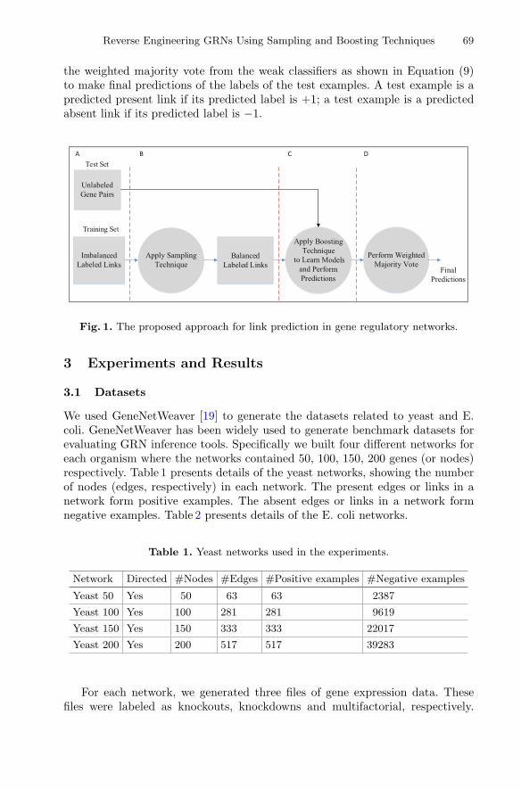
Figure 1 presents an overview of our approach. In (A), we are given a trainingset containing imbalanced labeled links. These labeled links include few posi-tive examples (i.e., known present links with labels of +1) and a lot of negativeexamples (i.e., known absent links with labels of −1). In addition, we are givena test set in which each test example is an unlabeled ordered gene pair. We con-struct feature vectors for both training examples and test examples as describedin Sect. 2.2. In (B), we apply a sampling technique, either under-sampling asdescribed in Sect. 2.3 or over-sampling as described in Sect. 2.4, to the trainingset to obtain a balanced training set. In (C), we apply a boosting techniqueas described in Sect. 2.5 to the balanced training set to learn K models (weakclassifiers). These models predict the labels of the test examples. In (D), we take


the weighted majority vote from the weak classifiers as shown in Equation (9)to make final predictions of the labels of the test examples. A test example is apredicted present link if its predicted label is +1; a test example is a predictedabsent link if its predicted label is −1.

Unlabeled Gene Pairs

Test Set

Final Predictions

A B

Balanced Labeled Links

C D

Training Set

Fig. 1. The proposed approach for link prediction in gene regulatory networks.

3 Experiments and Results

3.1 Datasets

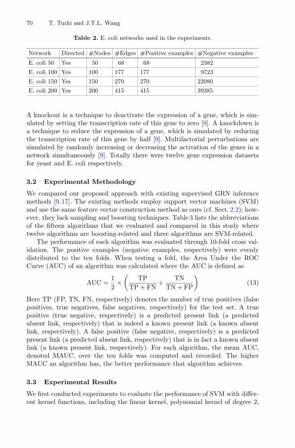
We used GeneNetWeaver [19] to generate the datasets related to yeast and E.coli. GeneNetWeaver has been widely used to generate benchmark datasets forevaluating GRN inference tools. Specifically we built four different networks foreach organism where the networks contained 50, 100, 150, 200 genes (or nodes)respectively. Table 1 presents details of the yeast networks, showing the numberof nodes (edges, respectively) in each network. The present edges or links in anetwork form positive examples. The absent edges or links in a network formnegative examples. Table 2 presents details of the E. coli networks.

Table 1. Yeast networks used in the experiments.

Network Directed #Nodes #Edges #Positive examples #Negative examples

Yeast 50 Yes 50 63 63 2387

Yeast 100 Yes 100 281 281 9619

Yeast 150 Yes 150 333 333 22017

Yeast 200 Yes 200 517 517 39283

For each network, we generated three files of gene expression data. Thesefiles were labeled as knockouts, knockdowns and multifactorial, respectively.


Table 2. E. coli networks used in the experiments.

Network Directed #Nodes #Edges #Positive examples #Negative examples

E. coli 50 Yes 50 68 68 2382

E. coli 100 Yes 100 177 177 9723

E. coli 150 Yes 150 270 270 22080

E. coli 200 Yes 200 415 415 39385

A knockout is a technique to deactivate the expression of a gene, which is sim-ulated by setting the transcription rate of this gene to zero [9]. A knockdown isa technique to reduce the expression of a gene, which is simulated by reducingthe transcription rate of this gene by half [9]. Multifactorial perturbations aresimulated by randomly increasing or decreasing the activation of the genes in anetwork simultaneously [9]. Totally there were twelve gene expression datasetsfor yeast and E. coli respectively.

3.2 Experimental Methodology

We compared our proposed approach with existing supervised GRN inferencemethods [9,17]. The existing methods employ support vector machines (SVM)and use the same feature vector construction method as ours (cf. Sect. 2.2); how-ever, they lack sampling and boosting techniques. Table 3 lists the abbreviationsof the fifteen algorithms that we evaluated and compared in this study wheretwelve algorithms are boosting-related and three algorithms are SVM-related.

The performance of each algorithm was evaluated through 10-fold cross val-idation. The positive examples (negative examples, respectively) were evenlydistributed to the ten folds. When testing a fold, the Area Under the ROCCurve (AUC) of an algorithm was calculated where the AUC is defined as

AUC =12

×(

TPTP + FN

+TN

TN + FP

)(13)

Here TP (FP, TN, FN, respectively) denotes the number of true positives (falsepositives, true negatives, false negatives, respectively) for the test set. A truepositive (true negative, respectively) is a predicted present link (a predictedabsent link, respectively) that is indeed a known present link (a known absentlink, respectively). A false positive (false negative, respectively) is a predictedpresent link (a predicted absent link, respectively) that is in fact a known absentlink (a known present link, respectively). For each algorithm, the mean AUC,denoted MAUC, over the ten folds was computed and recorded. The higherMAUC an algorithm has, the better performance that algorithm achieves.

3.3 Experimental Results

We first conducted experiments to evaluate the performance of SVM with differ-ent kernel functions, including the linear kernel, polynomial kernel of degree 2,


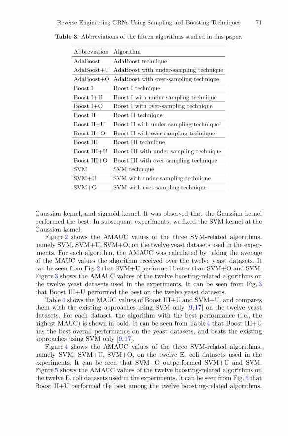
Table 3. Abbreviations of the fifteen algorithms studied in this paper.

Abbreviation Algorithm

AdaBoost AdaBoost technique

AdaBoost+U AdaBoost with under-sampling technique

AdaBoost+O AdaBoost with over-sampling technique

Boost I Boost I technique

Boost I+U Boost I with under-sampling technique

Boost I+O Boost I with over-sampling technique

Boost II Boost II technique

Boost II+U Boost II with under-sampling technique

Boost II+O Boost II with over-sampling technique

Boost III Boost III technique

Boost III+U Boost III with under-sampling technique

Boost III+O Boost III with over-sampling technique

SVM SVM technique

SVM+U SVM with under-sampling technique

SVM+O SVM with over-sampling technique

Gaussian kernel, and sigmoid kernel. It was observed that the Gaussian kernelperformed the best. In subsequent experiments, we fixed the SVM kernel at theGaussian kernel.

Figure 2 shows the AMAUC values of the three SVM-related algorithms,namely SVM, SVM+U, SVM+O, on the twelve yeast datasets used in the exper-iments. For each algorithm, the AMAUC was calculated by taking the averageof the MAUC values the algorithm received over the twelve yeast datasets. Itcan be seen from Fig. 2 that SVM+U performed better than SVM+O and SVM.Figure 3 shows the AMAUC values of the twelve boosting-related algorithms onthe twelve yeast datasets used in the experiments. It can be seen from Fig. 3that Boost III+U performed the best on the twelve yeast datasets.

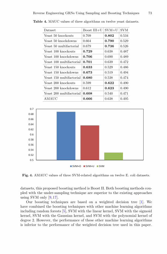
Table 4 shows the MAUC values of Boost III+U and SVM+U, and comparesthem with the existing approaches using SVM only [9,17] on the twelve yeastdatasets. For each dataset, the algorithm with the best performance (i.e., thehighest MAUC) is shown in bold. It can be seen from Table 4 that Boost III+Uhas the best overall performance on the yeast datasets, and beats the existingapproaches using SVM only [9,17].

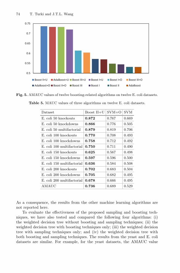
Figure 4 shows the AMAUC values of the three SVM-related algorithms,namely SVM, SVM+U, SVM+O, on the twelve E. coli datasets used in theexperiments. It can be seen that SVM+O outperformed SVM+U and SVM.Figure 5 shows the AMAUC values of the twelve boosting-related algorithms onthe twelve E. coli datasets used in the experiments. It can be seen from Fig. 5 thatBoost II+U performed the best among the twelve boosting-related algorithms.


0.45

0.47

0.49

0.51

0.53

0.55

0.57

0.59

0.61

0.63

0.65

SVM+U SVM+O SVM

Fig. 2. AMAUC values of three SVM-related algorithms on twelve yeast datasets.

0.45

0.5

0.55

0.6

0.65

0.7

Boost III+U Boost I+U Boost II+U AdaBoost+U Boost I+O Boost III+O

Boost III Boost II Adaboost Boost I Boost II+O AdaBoost+O

Fig. 3. AMAUC values of twelve boosting-related algorithms on twelve yeast datasets.

Table 5 shows the MAUC values of Boost II+U and SVM+O, and comparesthem with the existing approaches using SVM only [9,17] on the twelve E. colidatasets. It can be seen from Table 5 that Boost II+U has the best overallperformance on the E. coli datasets, and beats the existing approaches usingSVM only [9,17].

To summarize, one of our proposed boosting methods coupled with the under-sampling technique achieves the best performance among all the fifteen algo-rithms studied in this paper on the yeast and E. coli datasets respectively. Forthe yeast datasets, this proposed boosting method is Boost III. For the E. coli


Table 4. MAUC values of three algorithms on twelve yeast datasets.

Dataset Boost III+U SVM+U SVM

Yeast 50 knockouts 0.709 0.802 0.534

Yeast 50 knockdowns 0.664 0.790 0.529

Yeast 50 multifactorial 0.679 0.736 0.526

Yeast 100 knockouts 0.729 0.638 0.487



Yeast 150 knockouts 0.633 0.529 0.486



Yeast 200 knockouts 0.599 0.622 0.490



AMAUC 0.666 0.638 0.495

0.5

0.52

0.54

0.56

0.58

0.6

0.62

0.64

0.66

0.68

0.7

SVM+O SVM+U SVM

Fig. 4. AMAUC values of three SVM-related algorithms on twelve E. coli datasets.

datasets, this proposed boosting method is Boost II. Both boosting methods cou-pled with the under-sampling technique are superior to the existing approachesusing SVM only [9,17].

Our boosting techniques are based on a weighted decision tree [1]. Wehave combined the boosting techniques with other machine learning algorithmsincluding random forests [5], SVM with the linear kernel, SVM with the sigmoidkernel, SVM with the Gaussian kernel, and SVM with the polynomial kernel ofdegree 2. However, the performance of these other machine learning algorithmsis inferior to the performance of the weighted decision tree used in this paper.


0.5

0.55

0.6

0.65

0.7

0.75

Boost II+U AdaBoost+U Boost III+U Boost I+U Boost I+O Boost III+O

AdaBoost+O Boost II+O Boost III Boost I Boost II AdaBoost

Fig. 5. AMAUC values of twelve boosting-related algorithms on twelve E. coli datasets.

Table 5. MAUC values of three algorithms on twelve E. coli datasets.

Dataset Boost II+U SVM+O SVM

E. coli 50 knockouts 0.872 0.767 0.669

E. coli 50 knockdowns 0.866 0.776 0.505

E. coli 50 multifactorial 0.879 0.819 0.706

E. coli 100 knockouts 0.770 0.708 0.493



E. coli 150 knockouts 0.625 0.567 0.498



E. coli 200 knockouts 0.702 0.683 0.504



AMAUC 0.736 0.689 0.529

As a consequence, the results from the other machine learning algorithms arenot reported here.

To evaluate the effectiveness of the proposed sampling and boosting tech-niques, we have also tested and compared the following four algorithms: (i)the weighted decision tree without boosting and sampling techniques; (ii) theweighted decision tree with boosting techniques only; (iii) the weighted decisiontree with sampling techniques only; and (iv) the weighted decision tree withboth boosting and sampling techniques. The results from the yeast and E. colidatasets are similar. For example, for the yeast datasets, the AMAUC value


for the weighted decision tree without boosting and sampling techniques is 0.45.This is lower than the existing approaches using SVM only (with AMAUC being0.495 as shown in Table 4). When the weighted decision tree is coupled with onlythe Boost III technique, its AMAUC value is 0.53. When the weighted decisiontree is coupled with only the under-sampling technique, its AMAUC value is0.61. When the weighted decision tree is coupled with both Boost III and under-sampling techniques, its AMAUC value is 0.666 as shown in Table 4, which ismuch higher than the AMAUC value of 0.45 achieved by the weighted decisiontree without boosting and sampling techniques.

4 Conclusion and Future Work

In this paper we present a new approach to gene network inference throughregulatory link prediction. Our approach uses a weighted decision tree as the baselearning algorithm coupled with sampling and boosting techniques to improveprediction performance. Experimental results demonstrated the superiority ofthe proposed approach over existing methods [9,17], and the effectiveness of oursampling and boosting techniques.

Moving forward, we are extending the techniques described here to miRNA-mediated regulatory networks. In addition to their importance as regulatoryelements in gene expression, the capacity of miRNAs to be transported from cellto cell implicates them in a panoply of pathophysiological processes that includeantiviral defense, tumorigenesis, lipometabolism and glucose metabolism [25,26].This role in disease complicates our understanding of translational regulationvia endogenous miRNAs. In addition, miRNAs seem to be present in differ-ent types of foods with potential implications on human health and disease.Understanding the biogenesis, transport and mechanisms of action of miRNAson their target genes would result in possible therapies. Thus, reverse engineer-ing of miRNA-mediated regulatory networks would contribute to human healthimprovement and disease treatment. We are exploring new ways for inferringsuch networks. We are also investigating other algorithms such as guided reg-ularized random forests (GRRF) [7,24] and compare them with the weighteddecision tree employed here.

References

1. Alhammady, H., Ramamohanarao, K.: Using emerging patterns to constructweighted decision trees. IEEE Trans. Knowl. Data Eng. 18(7), 865–876 (2006)

2. Altaf-Ul-Amin, M., Afendi, F.M., Kiboi, S.K., Kanaya, S.: Systems biology in thecontext of big data and networks. In: BioMed Research International 2014 (2014)

3. Altaf-Ul-Amin, M., Katsuragi, T., Sato, T., Kanaya, S.: A glimpse to backgroundand characteristics of major molecular biological networks. In: BioMed ResearchInternational 2015 (2015)

4. Batista, G.E., Prati, R.C., Monard, M.C.: A study of the behavior of several meth-ods for balancing machine learning training data. ACM SIGKDD Explor. Newslett.6(1), 20–29 (2004)


5. Breiman, L., Friedman, J., Stone, C.J., Olshen, R.A.: Classification and RegressionTrees. CRC Press, New York (1984)

6. Bunkhumpornpat, C., Sinapiromsaran, K., Lursinsap, C.: Safe-Level-SMOTE:safe-level-synthetic minority over-sampling technique for handling the class imbal-anced problem. In: Theeramunkong, T., Kijsirikul, B., Cercone, N., Ho, T.-B. (eds.)PAKDD 2009. LNCS, vol. 5476, pp. 475–482. Springer, Heidelberg (2009). doi:10.1007/978-3-642-01307-2 43

7. Deng, H., Runger, G.: Gene selection with guided regularized random forest. Pat-tern Recogn. 46(12), 3483–3489 (2013)

8. Freund, Y., Schapire, R.E.: A desicion-theoretic generalization of on-line learningand an application to boosting. In: Vitanyi, P. (ed.) EuroCOLT 1995. LNCS, vol.904, pp. 23–37. Springer, Heidelberg (1995). doi:10.1007/3-540-59119-2 166

9. Gillani, Z., Akash, M., Rahaman, M., Chen, M.: CompareSVM: supervised, supportvector machine (SVM) inference of gene regularity networks. BMC Bioinformatics15, 395 (2014). http://dx.doi.org/10.1186/s12859-014-0395-x

10. He, H., Garcia, E.A.: Learning from imbalanced data. IEEE Trans. Knowl. DataEng. 21(9), 1263–1284 (2009)

11. He, H., Ma, Y.: Imbalanced Learning: Foundations, Algorithms, and Applications.Wiley, Piscataway (2013)

12. Ideker, T., Krogan, N.J.: Differential network biology. Mol. Syst. Biol. 8(1), 565(2012)

13. Kibinge, N., Ono, N., Horie, M., Sato, T., Sugiura, T., Altaf-Ul-Amin, M., Saito,A., Kanaya, S.: Integrated pathway-based transcription regulation network miningand visualization based on gene expression profiles. J. Biomed. Inform. 61, 194–202(2016)

14. Leclerc, R.D.: Survival of the sparsest: robust gene networks are parsimonious.Mol. Syst. Biol. 4(1), 213 (2008)

15. Liu, X.Y., Wu, J., Zhou, Z.H.: Exploratory undersampling for class-imbalancelearning. IEEE Trans. Syst. Man Cybern. Part B (Cybern.) 39(2), 539–550 (2009)

16. Margolin, A.A., Wang, K., Lim, W.K., Kustagi, M., Nemenman, I., Califano, A.:Reverse engineering cellular networks. Nat. Protoc. 1(2), 662–671 (2006)

17. Mordelet, F., Vert, J.P.: SIRENE: supervised inference of regulatory net-works. Bioinformatics 24(16), i76–i82 (2008). http://bioinformatics.oxfordjournals.org/content/24/16/i76.abstract

18. Patel, N., Wang, J.T.L.: Semi-supervised prediction of gene regulatory net-works using machine learning algorithms. J. Biosci. 40(4), 731–740 (2015).http://dx.doi.org/10.1007/s12038-015-9558-9

19. Schaffter, T., Marbach, D., Floreano, D.: GeneNetWeaver: in silico benchmarkgeneration and performance profiling of network inference methods. Bioinformatics27(16), 2263–2270 (2011)

20. Turki, T., Bassett, W., Wang, J.T.L.: A learning framework to improve unsuper-vised gene network inference. In: Perner, P. (ed.) MLDM 2016. LNCS (LNAI), vol.9729, pp. 28–42. Springer, Cham (2016). doi:10.1007/978-3-319-41920-6 3

21. Turki, T., Ihsan, M., Turki, N., Zhang, J., Roshan, U., Wei, Z.: Top-k parame-trized boost. In: Prasath, R., O’Reilly, P., Kathirvalavakumar, T. (eds.) MIKE2014. LNCS (LNAI), vol. 8891, pp. 91–98. Springer, Cham (2014). doi:10.1007/978-3-319-13817-6 10

22. Turki, T., Wang, J.T.L.: A new approach to link prediction in gene regulatorynetworks. In: Jackowski, K., Burduk, R., Walkowiak, K., Wozniak, M., Yin, H.(eds.) IDEAL 2015. LNCS, vol. 9375, pp. 404–415. Springer, Cham (2015). doi:10.1007/978-3-319-24834-9 47

http://dx.doi.org/10.1007/978-3-642-01307-2_43

http://dx.doi.org/10.1007/978-3-642-01307-2_43

http://dx.doi.org/10.1007/3-540-59119-2_166

http://dx.doi.org/10.1186/s12859-014-0395-x

http://bioinformatics.oxfordjournals.org/content/24/16/i76.abstract

http://bioinformatics.oxfordjournals.org/content/24/16/i76.abstract

http://dx.doi.org/10.1007/s12038-015-9558-9

http://dx.doi.org/10.1007/978-3-319-41920-6_3

http://dx.doi.org/10.1007/978-3-319-13817-6_10

http://dx.doi.org/10.1007/978-3-319-13817-6_10

http://dx.doi.org/10.1007/978-3-319-24834-9_47

http://dx.doi.org/10.1007/978-3-319-24834-9_47


23. Turki, T., Wang, J.T.L., Rajikhan, I.: Inferring gene regulatory networks by com-bining supervised and unsupervised methods. In: 15th IEEE International Confer-ence on Machine Learning and Applications, ICMLA 2016, Anaheim, CA, USA,18–20 December 2016

24. Wang, S., Yao, X.: Relationships between diversity of classification ensembles andsingle-class performance measures. IEEE Trans. Knowl. Data Eng. 25(1), 206–219(2013). http://dx.doi.org/10.1109/TKDE.2011.207

25. Zhong, L., Wang, J.T.L., Wen, D., Aris, V., Soteropoulos, P., Shapiro, B.A.: Effec-tive classification of microRNA precursors using feature mining and AdaBoostalgorithms. OMICS: J. Integr. Biol. 17(9), 486–493 (2013)

26. Zhong, L., Wang, J.T.L., Wen, D., Shapiro, B.A.: Pre-miRNA classification viacombinatorial feature mining and boosting. In: 2012 IEEE International Confer-ence on Bioinformatics and Biomedicine, BIBM 2012, Philadelphia, PA, USA, 4–7October 2012, Proceedings, pp. 1–4 (2012). http://doi.ieeecomputersociety.org/10.1109/BIBM.2012.6392700

http://dx.doi.org/10.1109/TKDE.2011.207

http://doi.ieeecomputersociety.org/10.1109/BIBM.2012.6392700

http://doi.ieeecomputersociety.org/10.1109/BIBM.2012.6392700

reverse engineering gene regulatory networks using ...wangj/publications/articles/mldm2017.pdf ·...

Documents