reverse-engineering the brain: a computer …...reverse-engineering the brain: a computer...

J E Smith

June 2018

Missoula, MT

[email protected]

Reverse-Engineering the Brain:

A Computer Architecture Grand Challenge

The Grand Challenge

June 2018 2copyright JE Smith

“The most powerful computing machine of all is the human brain.

Is it possible to design and implement an architecture that

mimics the way the human brain works?”

-- Workshop report: Mary J. Irwin and John P. Shen, “Revitalizing computer architecture

research,” Computing Research Association (2005).

Introduction

❑ The human brain is capable of:

• Accurate sensory perception

• High level reasoning and problem solving

• Driving complex motor activity

❑ With some very impressive features:

• Highly energy efficient

• Flexible – supports a wide variety of cognitive functions

• Learns dynamically, quickly, and simultaneously with operation

❑ Far exceeds anything conventional machine learning has achieved

• Will the trajectory of conventional machine learning ever achieve the same capabilities?

• OR should we seek new approaches based on the way the brain actually works?

❑ After the tutorial, it is hoped that attendees will:

• Understand the nature of the problem,

• View it as a computer architecture research problem,

• Have a firm foundation for initiating study of the problem,

• Participate in a serious effort to tackle the grand challenge.


Computer Architecture Perspective


❑ This research is at the intersection of

computer architecture, theoretical

neuroscience, and machine learning

• It is of major importance to all three

• And it requires knowledge of all three

❑ Most researchers are likely to rooted in

one of them

• This will shape the perspective and

direction of the research

❑ Our perspective (and biases) come from

computer architecture

• We should tackle the problem from our

perspective, using our background and

strengthsMachine Learning

ComputerArchitecture

TheoreticalNeuroscience

Reverse-Engineering the Brain

Macro-Columns

Lobes

Region Hierarchy

Neocortex

Feedforward/Micro-Columns

Model Neurons

Biological Neurons

❑ “Reverse-abstracting the neocortex” is a better way to put it

• The neocortex is the part of the brain we are interested in

• Reverse-abstracting is discovering the layers of

abstraction, bottom-up

What does “Reverse-Engineering the Brain” mean?


Combinational/RTL

Machine Language Software

Logic gates

Application Software

Processor Core + Memory

Block Hierarchy

HLL Procedure Hierarchy

Physical CMOS

Current Research

Neuro Architecture Stack

Silicon Architecture Stack

Science v. Architecture


❑ Consider two implementations of the brain’s computing

paradigm:

• Biological implementation that we each possess

• Human-engineered, silicon-based implementation that we

would like to achieve

❑ From the neuroscience perspective:

• Goal: Discover ever greater and more accurate information

regarding biological processes

❑ From a computer architecture perspective:

• Goal: Discover a new computational paradigm

❑ Differences in goals may lead to different approaches

Macro-Columns

Lobes

Region Hierarchy

Neocortex


Model Neurons

Biological Neurons

Outline

❑ Introductory Remarks

❑ Research Focus: Milestone TNN

• Classification and Clustering

• Neural Network Taxonomy

❑ Biological Background

• Overview

• Neural Information Coding

• Sensory Encoding

❑ Fundamental Hypotheses

• Theory: Time as a Resource

❑ Low Level Abstractions

• Excitatory Neuron Models

• Modeling Inhibition

❑ Column Architecture

❑ Case Studies

• Recent TNNs

❑ Space-Time Theory and Algebra

❑ Implementations

• Indirect Implementations: Simulation

• Direct Implementations: Neuromorphic Circuits

❑ Concluding Remarks


Research Focus: Milestone Network

Milestone Temporal Neural Network (TNN)

❑ We are attempting to solve a huge problem

❑ Reduce it to “bite-size” pieces

• This is the first “bite”

❑ Feedforward clustering networks (unsupervised training)

• Most current neuroscientific TNN projects have this target

❑ Sufficient for:

• Demonstrating TNN capabilities, and

• Exposing major differences wrt conventional machine learning methods

June 2018 copyright JE Smith 9

First, some background

Spike Communication


❑ Consider systems where information

is communicated via transient events

• e.g., voltage spikes

❑ Method 1: values are encoded as

spike rates measured on individual

lines

❑ Changing spikes on one line only

effects values on that line

❑ Method 2: values are encoded as

temporal relationships across parallel

communication lines

❑ Changing spikes on one line may

effect values on any/all of the others

The temporal communication method has

significant, broad experimental support

• The rate method does not.

• (Much) more later

rates

8

2

5

4

spike trains

time

values encoded as spike

times relative to t=0 0

6

3

4

t = 0

precise timing

relationships

time

Temporal Coding



times relative to t =0 0

6

3

4t = 0

precise timing

relationships

time

❑ Use relative timing relationships across multiple parallel lines to

encode information

❑ Changing the spike time on a given line may affect values on any/all

the other lines

Temporal Coding



times relative to t =0 2

3

0

1= t 0

precise timing

relationships

time

❑ Use relative timing relationships across multiple parallel spikes to

encode information

❑ Changing the spike time on a given line may affect values on any/all

the other lines

Plot on Same (Plausible) Time Scale


Temporal method is

An order of magnitude faster

An order of magnitude more

efficient (#spikes)

10 msec

Spike Computation


❑ Temporal Neural Networks

• Networks of functional blocks whose input and output values are communicated via

precise timing relationships (expressed as spikes)

• Feedforward flow (without loss of computational generality)

• Computation: a single wave of spikes passes from inputs to outputs

❑ A critical first step

• At the forefront of current theoretical neuroscience

.

.

.

Input

Val

ues

Encode

to

Spikes

Decode

from

Spikes

F1

F4

F5

Fn

Fn-2

F2

F3

Fn-1

.

.

.

x1

x2

xm

z2

zp

z16

7

4

9

12

6269

75

Ou

tpu

t Valu

es

...

...

...

...

...

...

.

.

.

.

.

.

.

.

.

0

1

2

3

60

57

Functional Block Features


1) Total function w/ finite implementation

2) Asynchronous

• Begin computing when the first spike arrives

3) Causal

• The output spike time is independent of any later input spike times

4) Invariant

• If all the input spike times are increased by some constant then the output

spike time increases by the same constant

⇒ Functional blocks interpret input values according to local time frames

F3

4

...

...

...

1

3

...

9 F3

3

...

...

...

0

2

...

8invariance

global time local time

Compare with Conventional Machine Learning

aka the Bright Shiny Object

❑ Three major processes:

• Training (Learning)

• Evaluation (Inference)

• Re-Training


Conventional Machine Learning: Training

❑ Training process

• Apply lots and lots of training inputs, over and over again


sequence of training patterns

MetaData (labels)

expected output patterns

Compareback propagate;adjust weights

Classifier Networkoutput

patterns

HUGELY expensive and

time-consuming

Training requires

labeled data

Conventional Machine Learning: Evaluation (Inference)

❑ Evaluation process:

• Apply input patterns, and compute output classes via vector inner

products (inputs . weights).


sequence of input patterns

compute output patterns via inner products w/ weights

Classifier Network

sequence ofoutput

classifications

Conventional Machine Learning: Re-Training

❑ If the input patterns change over time, perhaps abruptly, the training

process must be re-done from the beginning

• Apply lots and lots of training inputs, over and over again


sequence of training patterns

MetaData (labels)

expected output patterns

Compareback propagate;adjust weights

Classifier Networkoutput

patterns

HUGELY expensive and

time-consuming

Training requires

labeled data

Milestone Temporal Neural Network

❑ Perform unsupervised clustering

• Not supervised classification

❑ Informally: A cluster is a group of similar input patterns

• It’s a grouping of input patterns based on implementation-defined intrinsic similarities

❑ A clustering neural network maps input patterns into cluster identifiers

• Note: some outlier patterns may belong to no cluster



❑ Each cluster has an associated

cluster identifier

• A concise output pattern that

identifies a particular cluster

• If there are M clusters, then there

are M cluster identifiers.

❑ The exact mapping of cluster

identifiers to clusters is

determined by the implementation

• A direct by-product of

unsupervised training

(there are no meta-data inputs)



Clustering Temporal Neural Network

sequence ofoutput cluster

identifiers

Evaluate cluster identifiers via non-

binary combinatorial networks

Train via adjusting weights at local

neuron level

Re-train via constantly re-adjusting weights at

local neuron level


❑ For outputs to be directly understood by humans, we must map cluster

identifiers into known labels (decoding)

• Via construction of a trivial classifier at the output

❑ The “similarity” metric is implied by the implementation

• Not an a priori, designer-supplied metric

❑ Network designer can control the maximum number of clusters





identifiers




neuron level


local neuron level




identifiers




neuron level


local neuron level

Summary: Milestone Temporal Neural Network

❑ Everything is done by the same

network concurrently

• Training

• Evaluation

• Re-training

❑ Training

• Unsupervised

• Always active

• Performed locally at each neuron

(synapse, actually)

❑ Evaluation

• Concurrent with training

• Tightly integrated with training


Temporal Neural Network as a Classifier

❑ First: train unsupervised via


• Synaptic weight training is

localized and efficient

❑ Turn off TNN training

❑ Train output decoder

• Maps cluster id’s to classes

• Trivial classifier, e.g., 1-to-1

mapping





identifiers

Evaluate cluster identifiers via non-binary combinatorial networks

Train via adjusting weights at local neuron level

Train trivial classifier to map cluster id s to classes

MetaData (labels)




identifiers

Map cluster id s to classes

Evaluate cluster identifiers via non-binary combinatorial networks

sequence ofclassifications

❑ Evaluate with training

disabled

Milestone Architecture Objectives

❑ Function:

• Encodes information as transient temporal events (e.g., voltage spikes)

• Groups input patterns into clusters based on similarity

• Input stream of patterns produces output stream of very simple cluster

identifiers

• Makes local synaptic weight adjustments concurrent with operation:

changes in input patterns cause changes to clustering

❑ Implementation Features:

• Simple computational elements (neurons) that operate very quickly and

energy efficiently

• Implementable with conventional CMOS circuitry


Demonstrate brain-like capabilities and efficiencies with silicon technology

A Good Starting Point: MNIST Benchmark

❑ A Goldilocks Benchmark

• Not too large, not too small

• Not too hard, not too easy

• Just right


❑ What it is:

• Tens of thousands of 28 x 28 grayscale images of written numerals 0-9

• Originally hand-written zip codes

• Labeled: 60K training patterns; 10K evaluation patterns

http://yann.lecun.com/exdb/mnist/

Neural Network Taxonomy


Virtually every machine

learning method in use today –

deep convolutional nets,

RBMs, etc.

Eliasmith et al. 2012 (Spaun)

Recent ETH papers

Brader et al. 2007

Diehl and Cook, 2015

O’Connor et al. 2015

Beyeler et al. 2013 (UC Irvine, GPU)

Querlioz et al., 2013 (memristors)

Maass 1999

Thorpe and Imbert 1989

Masquelier and Thorpe 2007

Kheradpisheh, Ganjtabesh, Masquelier 2016

Natschläger and Ruf 1998 (RBF neurons)

Probst, Maass, Markram, Gewaltig 2012

(Liquid State Machines)

Neural Networks

rate theory

ANNs

temporal theory

spike

implementation

RNNs TNNs

rate

implementationspike

implementation

SNNs

rate

abstraction

8

2

5

4

spike train

spike times relative to t=0 encode values

0

6

3

4

t = 0

precise

timing

relationships

Distinguish computing model from SNN implementation

Neural Network Taxonomy


Subspecies

that can

hybridize

An entirely different genus

RNNs and TNNs are two very different models, both with SNN

implementations, and they should not be conflated

Neural Networks

rate theory

ANNs

temporal theory

spike

implementation

RNNs TNNs

rate

implementationspike

implementation

SNNs

Example: Conflating SNNs


Yann LeCun

August 7, 2014 · My comments on the IBM TrueNorth neural net chip.

IBM has an article in Science about their TrueNorth neural

net chip….

…

Now, what wrong with TrueNorth? My main criticism is that

TrueNorth implements networks of integrate-and-fire

spiking neurons. This type of neural net that has never

been shown to yield accuracy anywhere close to state of

the art on any task of interest (like, say recognizing objects

from the ImageNet dataset). Spiking neurons have binary

outputs (like neurons in the brain). The advantage of

spiking neurons is that you don't need multipliers (since the

neuron states are binary). But to get good results on a task

like ImageNet you need about 8 bit of precision on the

neuron states. To get this kind of precision with spiking

neurons requires to wait multiple cycles so the spikes

"average out". This slows down the overall computation.

…

This criticism assumes the RNN (rate) model and

correctly points out a major flaw.

HOWEVER, this criticism does not apply to TNNs

The two SNN-based models should not be conflated

TrueNorth is a platform upon which a wide variety

spiking neuron models (both RNNs and TNNs) can

be studied.

An implementation platform and a computing

model should not be conflated.

https://www.facebook.com/yann.lecun?hc_ref=ARTbn7P4cXUhYUWbG5bzBD49MV_3BBLL5Tfh8ayocDV1yA5ZaFiEsIecMMyZVj0k_7U&fref=nf

https://www.facebook.com/yann.lecun/posts/10152184295832143

Biological Background

Overview

The Brain

❑ Inner, “older” parts of the brain are responsible for automatic processes, basic

survival processes, emotions

• Not of interest for this line of research

❑ Neocortex

• The “new shell” that surrounds the older brain

• Performs the high level skills we are most interested in

sensory perception

cognition

intellectual reasoning

generating high level motor commands

• Our primary interest is the neocortex


from quora.com

❑ Hippocampus

• Responsible for memory formation and

sense of place

❑ Cerebellum

• Responsible for motor control

coordination

Neocortex


copyright 2009 Pearson Education, Inc

illustration of major regions and lobes

❑ Thin sheet of neurons

• 2 to 3 mm thick

• Area of about 2500 cm2

Folds increase surface area

• Approx 100 billion total neurons

(human)

❑ Hierarchical Physical Structure

• Lobes

• Regions

• Subregions, etc.

• Macro-Columns

• Micro-Columns

• Neurons

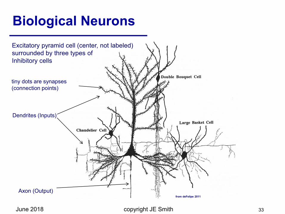
Biological Neurons

June 2018 33

from deFelipe 2011

Excitatory pyramid cell (center, not labeled)

surrounded by three types of

Inhibitory cells

tiny dots are synapses

(connection points)

Dendrites (Inputs)

Axon (Output)

copyright JE Smith

Neuron Operation


Synapse

Upstream

Neuron

Downstream

Neuron

Dendrites

Body

Dendrites

-70 mv

-55 mv

30 mvOutput Spike

time (msec)Axon

1 ms

100

mv

1 mv

10 ms

Excitatory Response

Spike

Body Potential

threshold

dendrites

symbol:

axon

body

Excitatory Neurons

June 2018 35

❑ About 80% of neurons are excitatory

❑ Most are pyramidal cells

• Axon reaches both near and far

• Capable of “precise” temporal operation

❑ Approximately 10K synapses per neuron

• Active connected pairs are far fewer than

physical connections suggest

90% or more are “silent” at any given time

• Multiple synapses per connected neuron pair

copyright JE Smith

100 μm

from Perin et al. 2011

Inhibitory Neurons

June 2018 36

from deFelipe 2011

❑ Inhibitory response functions have the opposite polarity

of excitatory response functions

• Reduce membrane potential and inhibit spike firing

❑ Also called “interneurons”

• Many types – most with exotic names

• Some are fast-spiking (electrical synapses)

• Others have slow response functions

❑ Less precise than excitatory neurons

❑ Act en masse on a local volume of neurons

• A “blanket” of inhibition

❑ Perform a number of tasks related to

• Maintaining stability

• Synchronization (via oscillations)

• Information filtering – emphasized in this tutorial

copyright JE Smith

[Karnani et al. 2014]Refs: [Markram et al. 2004]

Glial Cells

June 2018 37

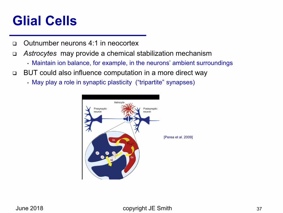
❑ Outnumber neurons 4:1 in neocortex

❑ Astrocytes may provide a chemical stabilization mechanism

• Maintain ion balance, for example, in the neurons’ ambient surroundings

❑ BUT could also influence computation in a more direct way

• May play a role in synaptic plasticity (“tripartite” synapses)

copyright JE Smith

[Perea et al. 2009]

Columnar Structure

June 2018 38

❑ Neurons are structurally organized as columns

between the top and bottom neocortical surfaces

❑ Columns are composed of layers

• Nominally 6, but it depends a lot on who is counting

❑ Micro-Columns (Mini-Columns)

• O(100 neurons) -- 80 excitatory; 20 inhibitory

• 64 excitatory and 16 inhibitory in the famous drawing

at right

[Mountcastle 1997]

from https://neuwritesd.org

copyright JE Smith

❑ Macro-Columns

• O(100s) micro-columns per macro-column

• In sensory systems, all micro-columns in a macro-

column map to same receptive field (RF)

• An RF may be a patch of retina or skin, or a rat’s

whisker

❑ Some theorists construct architectures using

the biological columnar structure as a guide

• Hawkins (On Intelligence) takes this approach

• This approach is not covered in this tutorial

Columnar Structure

June 2018 39

[Körner et al. 1999]

copyright JE Smith

Refs: [Hawkins and Blakeslee 2007] [Rinkus 2010]

[Oberlander et al. 2012]

from: http://www.kurzweilai.net

Summary

June 2018 40

[Felleman and Van Essen 1991]

Micro-Column

O(100) neurons

Macro-Column

O(100) micro-columns

Regions, Subregions

Many Macro-Columns

from Ramon y Cajal

(via wikipedia)

Neuron

[Mountcastle 1997][Hill et al. 2012]

copyright JE Smith

Uniformity Hypothesis

❑ Hypothesis: The structure and operation of the

neocortex is uniform

• Across species

• Across neocortical regions within a species

❑ “Uniform” is a subjective term

• It depends on the user’s perspective

❑ From our perspective: All cognitive processing

follows the same paradigm(s) as sensory

processing

• Why important? Most in vivo experimental data is for

sensory processing,

• Across a number of species

❑ So, by accepting uniformity, there is lots of useful

experimental data regarding the basic

paradigm(s) of cognitive processing


[DeFelipe et al. 2002] [Carlo and Stevens 2013]Refs: [Mountcastle 1997]

❑ Neuron latency

• 1’s of milliseconds per neuron

❑ Transmission delay

• Path lengths order (100s um)

• Prop. delay order (100s um per ms)

• 1’s of milliseconds between two neurons

❑ Multiple synapses per neuron pair

• On the order of 5 -10

Some Engineering Considerations


from Bakkum et al. 2008

from Hill et al. 2012

axons dendrites

from Hill et al. 2012 from Fauth et al. 2015

Low Resolution Data

❑ Biological materials and “hardware” structure support only low

resolution data

• 3-4 bits

❑ But that is OK

• A lot of information can be captured by low resolution values

• Consider 4-bit grayscale:


❑ Low resolution makes temporal encoding practical

• Because temporal encoding is a unary encoding

• Temporal encoding exploits time as an implementation resource

❑ Ultimately, low resolution signaling leads to low energy consumption


Neural Information Coding

Rate Coding

❑ Rate Coding: The name just about says it all

• The first thing a typical computer engineer would think of doing

• Consistent with neuron doctrine: spikes communicate information


rates

8

2

5

4

spike trains

time

Rate Coding

June 2018 46

❑ Early experimenters applied constant current to neuron body and observed:

copyright JE Smith

time

input current

pA

axon

potential

10s mv

2 3fr

eq

ue

ncy

(H

z)4 5 6 7 8 9 10

applied current (pA)

30

40

50

60

70

80

90

100

110

FI Curve

0 10 20 30 40 50 60 70

time (msec)

bo

dy

po

ten

tial (

mv)

30

-55

-70

frequency = 70 Hz @ 5 pA

❑ Such constant current responses are often

used to characterize neuron behavior

• Vary step amplitude ⇒ Frequency-Current

relationship (FI Curve)

❑ Appears to support rate coding

• The greater the input stimulus, the higher the

output spike rate

Temporal Coding


❑ Use relative timing relationships across multiple

parallel spikes to encode information



6

3

4

t = 0

precise timing

relationships

time

Key Experiment

❑ 100 msec is sufficient in most cases (80%)

❑ At least 10 neurons in series along feedforward path, each consuming ~10 msec

(communication + computation).

❑ Conclusion: Only first spike per line can be communicated this quickly

• Rates require a minimum of two spikes (probably several more)

• Temporal coding must be present


Image pathway from retina to IT, where image is identified

Retina LGN V1 V2 V4 IT

❑ Thorpe and Imbert (1989)

• Show subject image #1 for tens of msecs (varied)

• Immediately show subject image #2

• Ask subject to identify image #1

• Measure correct responses

from www.thebrain.mcgill.ca

from Thorpe & Imbert 1989

❑ Lee et al. (2010)

Input/Processing/Output Pathway

❑ Path length similar to Thorpe and Imbert ⇒ there is time only for first spikes

❑ Higher contrast spot ⇒ spikes occur sooner for stronger stimulus

❑ Statistically significant correlation between RT and NL

❑ No statistically significant correlation between FR and RT.


• Trained monkey fixes its gaze on a spot in the center of a screen

• A “dot” of variable contrast appears at a point away from the center

• If the monkey’s eyes immediately saccade to the new contrast spot,

• Monkey is rewarded and a data point is collected

Neural Latency (NL)

Target Onset

Response Time (RT)

Firing Rate (FR)Visual Cortex

LGN

Re

tina

Ca

na

l

Pause NeuronsBurst Neurons

Ocular Motoneurons

Visual Stimulus

(Local)

Visual Stimulus

(Global)

Head Rotation

Head Movements

Cerebral Cortex

Superior

Colliculus

Vest. N

OKR

VOR Eye Movements

NL – time from target onset to

spikes at V1

RT – time from target onset to

saccade

FR – spike firing rate at V1

It’s a Matter of Survival

❑ Any organism that relies on its senses for survival depends on fast

cognitive paths

❑ Experiments strongly suggest sensory input is communicated and

processed as a feedforward wavefront of precisely timed spikes

• This is a very fast and efficient way to communicate information

❑ Key question: Is this temporal communication paradigm used throughout

the entire neocortex?

Conjecture: Yes, especially considering uniformity hypothesis


Because it’s a matter of survival, this is probably the fastest, most efficient

cognitive method that evolution could devise. So wouldn’t evolution use it

everywhere as a basic technology?

Temporal Stability

Mainen and Sejnowski (1995)


• Repeatedly inject step current into neuron body

• Capture and analyze output spike trains

• Spike trains (10 trials); Raster plots (25 trials)

❑ Jitter ⇒ several spikes required

to establish a reliable rate

• Repeatedly inject realistic pseudorandom

current into neuron body

• Capture and analyze output spike train

❑ Spike times are very stable

“stimuli with fluctuations resembling synaptic activity produced spike

trains with timing reproducible to less than 1 millisecond”

step current realistic

current

Time Resolution

June 2018 52

❑ Petersen, Panzeri, and Diamond (2001)

• Somatosensory cortex of rat (barrel columns)

• Map a specific whisker to two cells in the receiving column

• Figure shows latency to first spike in response to whisker

stimulation

http://www.glycoforum.gr.jp/science/word/proteoglycan/PGA07E.html

units are .1 msec

copyright JE Smith

“82%–85% of the total information was contained in the timing of individual spikes: first

spike time was particularly crucial. Spike patterns within neurons accounted for the remaining

15%–18%.”

Information Content

❑ Kermany et al. (2010)


• In vitro culture of neurons

• Multi-grid array

• Five stimulation points

• Collect output spikes at least one

neuron removed from stimulation

point.

• Collect spike data for 100 msec

• Which was the stimulation point?

• Analyze data two ways for spike

timing:

time to first spike (TFS)

rank order

• Analyze two ways for rates:

total spikes

pop. count histogram (PCH)

• Use a conventional classifier to

determine the accuracies

❑ Time based reductions have higher accuracies (implying higher

information content)

Summary


❑ If you were selecting a technology and had these two choices, which

would you choose?

Temporal Coding Rate Coding

Fast enough? Yes No

Information content High Low

Energy consumption Low High

“When rephrased in a more meaningful way, the rate-based view

appears as an ad hoc methodological postulate, one that is practical

but with virtually no empirical or theoretical support.” -- Brette 2015


Encoding Sensory Input

Sensory Inputs


❑ Raw input values are “Sensory Inputs”

• They correspond to physical inputs from the biological senses

• In an artificial environment, we can also invent our own “senses”

E.g., Temperature sensors spread out over a grid

❑ Encoding translates sensory inputs to temporal code

• Vision: fairly straightforward, often used by theoreticians

• Auditory: uses frequency transform

• Olfactory: must learn/operate quickly over a very large feature space

• Somatosensory: extremely straightforward, has proven valuable to

experimentalists

• Place: an extremely interesting sense that is internally produced

• Generic: a grid of temperature sensors, for example

Visual Input


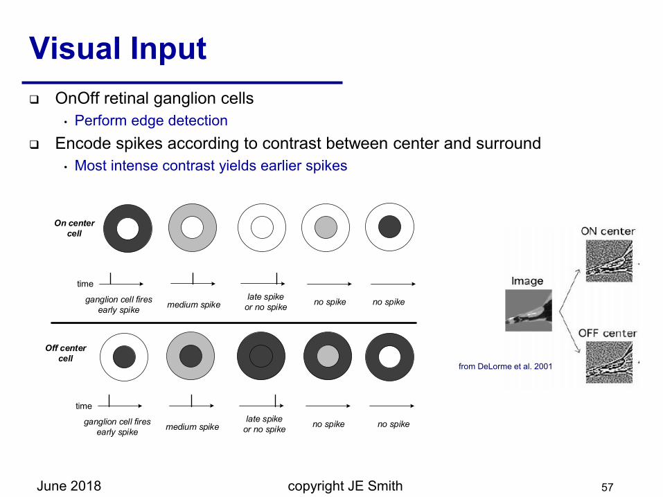
❑ OnOff retinal ganglion cells

• Perform edge detection

❑ Encode spikes according to contrast between center and surround

• Most intense contrast yields earlier spikes

from DeLorme et al. 2001

On center

cell

ganglion cell fires

early spike

time

Off center

cell

medium spikelate spike

or no spikeno spike no spike

ganglion cell fires

early spike

time

medium spikelate spike

or no spikeno spike no spike

Auditory Input


❑ Tiny hairs (cilia) at different locations in cochlea are sensitive to

different frequencies

• Hair cells perform frequency transform

• Most intense frequencies generate earlier spikes

from Angelo Farina via SlidePlayer.comfrom Lankamedicalaudio.com

Somatosensory Input


❑ Wide variety of receptor types

• Many are mechanical

❑ Rat whiskers are a prime example

• Highly developed, finely-tuned sensor in nocturnal rodents

• Generate spikes that correlate with degree of “whisking”

• The greater/faster the deflection, the sooner the spike

❑ Widely used by experimental researchers

• Each whisker is a receptive field which drives a particular macro-

column or “barrel column”

• This relationship permits well-controlled in vivo experiments

http://www.glycoforum.gr.jp/science/word/proteoglycan/PGA07E.html

Olfactory Input


❑ Olfactory receptor neurons (ORNs)

• Dendrites connect to tiny hairs containing

proteins that bind to odor molecules

• Stronger odor affinity causes earlier spike

❑ 10M ORNs in a human

• Proteins coded with 1000 different genes

❑ Must learn/operate quickly over a very

large feature space

• To deal with the unpredictability of the

olfactory world

❑ Low bandwidth

• In contrast: Vision is high bandwidth

• (Imagine reading a book where different

odors encode letters)

❑ See Laurent (1999)

from health.howstuffworks.com

Sense of Place


❑ The innate sense of where you are in space

– your “place”

❑ Does not have a physical world interface (unlike the other senses)

❑ Stored as macro-column grid in entorhinal cortex

• Hexagonal/triangular

• Located between neocortex and hippocampus

• Neurons fire as subject moves in space

❑ Aside: hippocampus is responsible for spatial memories & navigation

• A lot of theoreticians are interested in the Hippocampus

from placeness.com

Outline






• Overview









❑ Case Studies

• Recent TNNs


❑ Implementations





Fundamental Hypotheses

Neuron Doctrine

❑ The neuron doctrine serves as the foundation for our enterprise

❑ A set of accepted principles (or laws) developed over a span of 100+ years

• Neurons are the atomic units of the brain’s structure and function

• Neurons consist of a body, dendrites, and axons

• Information is received at dendrites connected to the neuron body and information is

transmitted to other neurons via the axon (law of polarization)

(and others)

❑ Dale’s law: A given neuron drives only one synapse type: either all excitatory or

all inhibitory

❑ To this foundation, add several hypotheses:

• Uniformity Hypothesis (given earlier)

• Temporal Hypothesis

• Feedforward Hypothesis

• Reliability Hypothesis

❑ Caveat: these hypotheses are not universally accepted and are often implicit


Temporal Hypothesis


❑ Hypothesis: Temporal Coding is used in the neocortex

❑ Experimental results (given earlier) support this hypothesis

• Synopsis: temporal coding is much faster, much more efficient, and much

more plausible than rate coding.



6

3

4

t = 0

precise timing

relationships

time

Feedforward Hypothesis


❑ Feedforward nets have same intrinsic computing power as Feedback nets

• Feedback nets may be much much more efficient, but they can’t perform a

theoretically larger set of computations (in the Turing sense)

❑ Therefore, we study feedforward networks without losing any computational generality

If a feedback computation satisfies the discrete-ness and finite-ness constraints of Turing’s thesis

Then there is an equivalent feedforward computation

❑ Consider any computing network with feedback

• Can be recurrent ANN, RBM, HTM… almost

anything, really

feedforward

time

g

feedforward g

feedforwardffeedforward

f

f

g

X1

X2

X3

Δ

Δ

f(X3,g(X2,g(X1)))

feedforwardf(X3,g(X2,g(X1)))

time

f

g

X1,X2,X3

feedback

Aside: Synchronizing Rhythms

❑ If we add feedback, how might

synchronization be performed?

❑ There are no clocked storage elements

❑ Inhibitory oscillations

• Gamma rhythm: roughly 40-100 Hz

• 10-25 msec coding window

❑ This is per-neuron synchronization

• Like a pipeline w/ a single gate per stage

• Neuron feeding itself is easily handled

This is speculative

June 2018 68

saccade-like

events

per saccade

encoding

Cortical Theta Rhythm 4-10Hz

100-250 msec. period

Gamma Rhythm 40-100Hz

10-25 msec. period

copyright JE Smith

Refs: [Singer 2010] [Fries et al. 2007]

Fault Tolerance

❑ What does this logic network do?

June 2018 69

x3

x7

x1

x8

x5

x6

x2

x4

z1

z2

z3

z4

z5

z6

z7

z8

answer: half-adder w/ inverted outputs

fault-tolerant interwoven logic (quadded)

copyright JE Smith

Ref: [Tryon 1962]

Temporal Stability

❑ Relatively little variation (skew) in delays and latencies within regions of

closely communicating neurons

❑ Probably required, in the absence of clocked storage elements

• Over at least an entire excitatory column

More likely at least a macro-column

❑ Global skew may higher than local skews

• Skew within a column or macro-column may be less than between widely

separated columns

❑ There may be a web of locally interacting mechanisms that tune delays and

latencies to provide temporal uniformity

• Oscillatory inhibition may be an associated cause and/or effect

❑ These mechanisms probably add a lot of apparent complexity


Everything on this slide is speculative

Reliability Hypothesis

❑ The computing paradigm used in the neocortex is independent of

supporting fault-tolerant and temporal stability mechanisms.

• If reliability and temporal stability are perfect – then the paradigm

probably works better than with less reliable networks.

❑ We will assume:

• All circuits are completely reliable

• Temporal stability guarantees at least 3-bits of timing resolution


Summary of Hypotheses

❑ Neuron Doctrine

❑ Uniformity Hypothesis

❑ Temporal Hypothesis

❑ Feedforward Hypothesis

❑ Reliability Hypothesis


Summary: TNN Architecture Features

❑ Feedforward

❑ Intrinsically fault-tolerant

❑ Temporally stable


.

.

.

Input

Val

ues

Encode

to

Spikes

Decode

from

Spikes

F1

F4

F5

Fn

Fn-2

F2

F3

Fn-1

.

.

.

x1

x2

xm

z2

zp

z16

7

4

9

12

6269

75

Ou

tpu

t Valu

es

...

...

...

...

...

...

.

.

.

.

.

.

.

.

.

0

1

2

3

60

57

Theory: Time as a Resource

❑ The way deal with time when constructing digital systems:

(Assume unit delay gates)

Step 1: Synchronous Binary Logic


1) Input signals change

2) Wait for output signals to stabilize

<0,0,0,0> → <0,0,0,0>

0

0

0

0

0

0

0

0

❑ Again, with different input timing

We always get the same, “correct” answer

Synchronous Binary Logic, contd.


❑ Synchronized logic removes the effects of physical time

• Results do not depend on the actual delays along network paths

• Ditto for delay independent asynchronous logic (e.g., handshaking)

0

0

0

0

0

0

0

0

❑ Sherwood and Madhavan (2015)

❑ Process information encoded as relative edge times

Step 2: Race Logic


❑ Time is divided into discrete intervals (unit time)

❑ Input edge times encode input information (relative to first edge)

❑ Output edge times encode the result (relative to first edge)

Normalize

1

2

3

0

3 = 6 - 3

2 = 5 - 3

1 = 4 - 3

0 = 3 - 31

2

3

4

2

3

4

5

3

4

5

6

Input values are sorted at output

2

2

3

0

1

3

3

4

2

4

5

3

5

6

4

5

After

Normalization

3

2

2

0

Race Logic, contd.

❑ Same circuit, same signals, same everything as with synchronous method,

except network implements a much more powerful function

integer sort vs. <0,0,0,0> → <0,0,0,0>


❑ Again, with different input timing

Input values are sorted at output

same circuit sorts numbers of any size

The Temporal Resource

❑ The flow of time has the ultimate engineering advantages

• It is free – time flows whether we want it to or not

• It requires no space

• It consumes no energy

❑ Yet, we (humans) try to eliminate the effects of time when

constructing computer systems

• Synchronizing clocks & delay-independent asynchronous circuits

• This may be the best choice for conventional computing problems and

technologies

❑ How about natural evolution?

• Tackles completely different set of computing problems

• With a completely different technology

June 2018copyright JE Smith

79

The flow of time can be used effectively as a

communication and computation resource.

Step 3: Generalize Race Logic

❑ Each functional block is:

• Causal: time of output edge is only affected by earlier-occurring input edges.

• Invariant: shifting all input edge times by a uniform amount causes the output edge to

time shift by the same amount


.

.

.

.

.

.

.

.

.

.

.

.

.

.

.

. . .

x1x2

xm

z2

zp

z10

2

6

1

3

7

4

9

0

12 60

70

79

75

G1

G4

G5

Gn

Gn-2

G2

G3

Gn-1

59

Step 4: Generalize Transient Events

Nothing special about 1 → 0 edges…

Could use 0 → 1 edges

OR

pulses (spikes):


.

.

.

.

.

.

.

.

.

.

.

.

.

.

.

. . .

x1x2

xm

z2

zp

z10

2

6

1

3

7

4

90

12 60

70

79

75

G1

G4

G5

Gn

Gn-2

G2

G3

Gn-1

59

Step 5: Specialize Functional Blocks

❑ Function blocks can be spiking neurons

❑ This is a Temporal Neural Network (TNN)

• As envisaged by an important group of theoretical neuroscientists


.

.

.

.

.

.

N1

N4

N5

Nn

Nn-2

N2

N3

Nn-1

.

.

.

.

.

.

.

.

.

. . .

x1x2

xm

z2

zp

z10

2

6

1

3

7

4

90

12 60

57

70

79

75

Temporal Neural Networks (TNNs)


❑ Input spike times encode information (temporal coding)

❑ Input initiates a wave of spikes that sweeps forward through the network

• At most one spike per line per computation

❑ Output spike times encode result information

.

.

.

.

.

.

N1

N4

N5

Nn

Nn-2

N2

N3

Nn-1

.

.

.

.

.

.

.

.

.

. . .

x1

x2

xm

z2

zp

z1

Low Level Abstractions

Excitatory Neuron Models

Neuron Operation (Re-Visited)

June 2018 85

dendrites

symbol:

axon

copyright JE Smith

Synapse

Upstream

Neuron

Downstream

Neuron

Dendrites

Body

Dendrites

-70 mv

-55 mv

30 mvOutput Spike

time (msec)Axon

1 ms

100

mv

1 mv

10 ms

Excitatory Response

Spike

Body Potential

threshold

Spikes and Responses

❑ Spike followed by Response

• Two sides of electrical-chemical-electrical translation at synaptic gap

❑ Spike is very narrow

• Result of ions being actively moved along the axon

June 2018 86

1 ms

100 mv

axon dendritesynapse

1 mv

50 ms

Spike

Response

upstream

neuron

downstream

neuron

Information Flow

copyright JE Smith

❑ Response is much wider with much lower peak potential

• Rise and fall of neuron body potential

• Excitatory response shown

• Many nearly-simultaneous responses cross threshold &

produce output spike

~3-10 ms

Neuron Models

❑ Hodgkin-Huxley (1952)

• Nobel Prize

• Complex coupled differential equations

• Gold standard for biological accuracy

• But we are not interested biological

accuracy! (only plausibility)

• We want computational capability

❑ Leaky Integrate and Fire (LIF)

simplification


M dVt/dt = - (Vt -Vrest) – ((gtE(Vt - VE) – gt

I (Vt - VI) + Ib)/ gM

E dgtE/dt = -gt

E ; gtE = gt-1

E + ∑ gE wij

I dgtI/dt = -gt

I ; gtI = gt-1

I + ∑ gI wij

+

_

+

_

+

_

gI

gE

gM

VI

VE

Vrest

CM

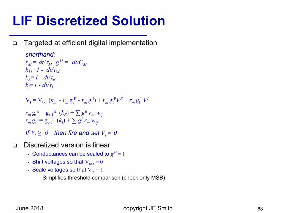
LIF Discretized Solution

❑ Targeted at efficient digital implementation

❑ Discretized version is linear• Conductances can be scaled to gM = 1

• Shift voltages so that Vrest = 0

• Scale voltages so that Vth = 1

Simplifies threshold comparison (check only MSB)


shorthand:

rM = dt/M gM = dt/CM

kM =1 - dt/M

kE=1 - dt/E

kI=1 - dt/I

Vt = Vt-1 (km - rm gtE - rm gt

I) + rm gtEVE + rm gt

I VI

rm gtE = gt-1

E (kE) + ∑ gE rm wij

rm gtI = gt-1

I (kI) + ∑ gI rm wij

If Vt ≥ then fire and set Vt = 0

LIF Digital Implementation


xE1(0/1)*W1

*W2

*Wn

xE2(0/1)

xEn(0/1)

∑

D1

D2

Dn

z(0/1)

E Synapse Adder

Vt

reset

∑

Membrane Adder

*KE

xI1(0/1)*W1

*W2

*Wm

xI2(0/1)

xIm(0/1)

∑

D1

D2

Dm

*KI

P

P

Excitatory Synapses

Inhibitory Synapses

P

Note: No refractory logic shown

gtE rm

Km = 1- gleak rm

gtI rm

threshold

check

1-gttot rmneg

neg ∑

Note: Scale values so that

threshold = 1.0

I Synapse Adder

Wi = wirm

Wi = wi gErm

g

Ex

g

In

VE

VI

[Smith 2014]

Excitatory Neuron Model

❑ A volley of spikes is applied at inputs

❑ At each input’s synapse, the spike produces a response function

• Synaptic weight (wi) determines amplitude: larger weight ⇒ higher amplitude

❑ Responses are summed linearly at neuron body

• Models the neuron’s membrane (body) potential

❑ Fire output spike if/when potential exceeds threshold value ()


response for high weight

response for lower weight

❑ Basic Spike Response Model (SRM0) -- Kistler, Gerstner, & van Hemmen (1997)

.

.

....

response

functions

w1

w2

wp

Σ

body potential

x2

x1

xp

y

input spikes synapses

Response Functions

❑ A wide variety of response functions are used

• Researchers’ choice

• Synaptic weight determines amplitude


Biexponential – most realistic

Non-leaky often used

Compound synapse has

skewed peak amplitude

Biexponential Piecewise linear

biexponential approximation

Original LIF

(Stein 1965) Non-leaky

Compound synapse Compound synapse

Non-leaky

Which Is the Approximation?


a) Biexponential spike

response

b) Piecewise linear spike

response

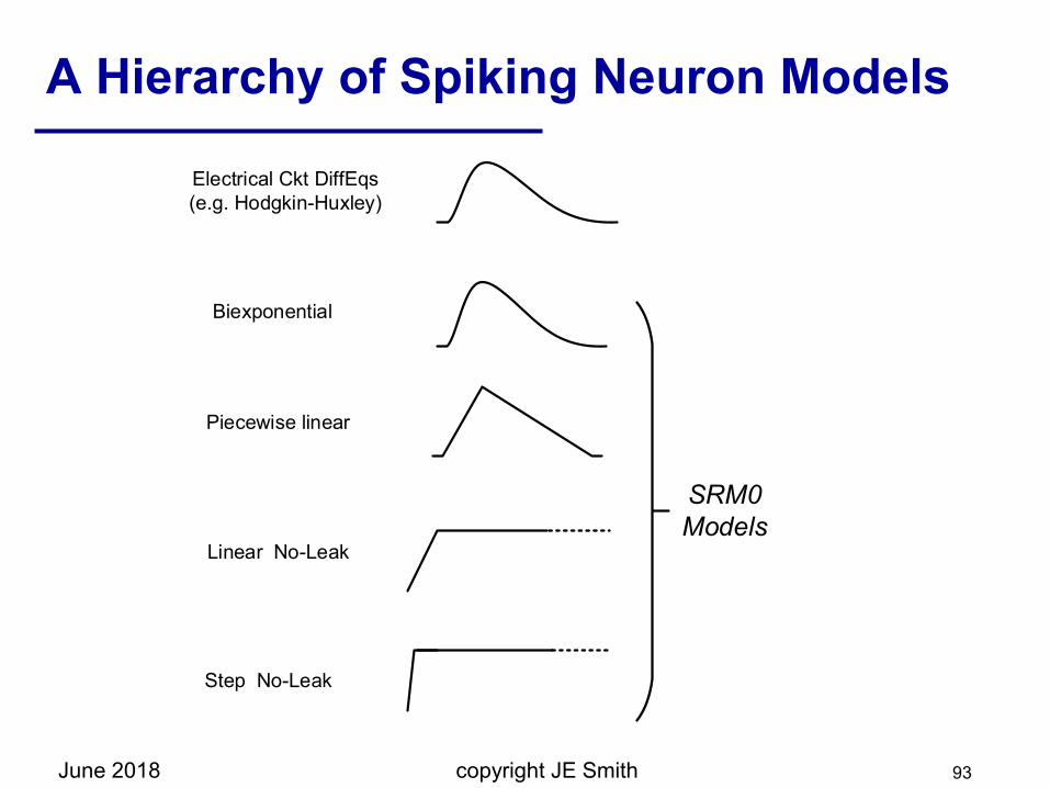
A Hierarchy of Spiking Neuron Models


Biexponential

Piecewise linear

Step No-Leak

Electrical Ckt DiffEqs

(e.g. Hodgkin-Huxley)

Linear No-Leak

SRM0

Models

Nomenclature: LIF Neuron Models

❑ Leaky Integrate-and-Fire

❑ Often mentioned in the literature

❑ A generic term for a broad class of neuron models

• Many neuron models leak, integrate, and fire

❑ Most SRM0 models are LIF

❑ When an LIF model is not SRM0, it is due to the leakage model


Terminology

❑ Physical connectivity

• A bundle is composed of multiple lines

❑ Information connectivity

• A volley consists of multiple spikes


Neuron Model: Synaptic Plasticity

❑ Synaptic weights determine a neuron’s overall function

❑ Hence, training synaptic weights is an essential part of the paradigm

❑ Bi and Poo (1998) provide experimental support

Additional Refs: [Markram et al. 1997] [Morrison et al. 2008]

June 2018 96

• In vitro rat hippocampal cells

• Probe pairs of synaptically

connected excitatory neurons

• Repetitively stimulate upstream

neuron at low frequency

• Measure downstream neuron

response (amplitude and spike time)

• Plot change in response amplitude

vs. Dt (time difference between

output and input spikes). Dt may be

pos. or neg.

copyright JE Smith

from Bi and Poo 1998

input spike after

output spike

input spike before

output spike

STDP

June 2018 97

❑ Spike Timing Dependent Plasticity :

• Compare relative input and output spike times

Input spike time < output spike time: associated synapse is potentiated

Input spike time output spike time: associated input synapse is depressed.

• Synaptic weights stabilize in a way that captures a neuron’s observed input patterns

_

D weight +

Dt

_

+depression

potentiation

tout tin

tin

Dt = tout – tin

tout

❑ Training is unsupervised, localized, and emergent

• This is a major difference wrt conventional error back-propagation

copyright JE Smith

from Bi and Poo 1998

STDP In Action

from Guyonneau, VanRullen, and Thorpe (2005)

Paraphrased

June 2018 98

• For a given input pattern, input spikes elicit an

output spike, triggering the STDP rule.

• Synapses carrying input spikes just preceding

the output spike are potentiated, while later

ones are weakened.

• The next time the input pattern is applied, the

firing threshold will be reached sooner, which

implies the output spike will occur sooner.

• Consequently, the STDP process, while

depressing some synapses it had previously

potentiated, will now reinforce different

synapses carrying even earlier spikes.

• By iteration, when the same input spike

pattern is repeated, the output spike time will

stabilize at a minimal value while the earlier

synapses become fully potentiated and later

ones fully depressed.

copyright JE Smith

8

0

8

0

weights

time

8

0

0

8

weights

time

8

0

4

4

weights

time

1) input spike shifts sooner 2) weight

adjusts upward

3) output spike shifts sooner

4) weight adjusts downward

Example


❑ Three input neuron

❑ Train for a single pattern

❑ Apply evaluation inputs

Response function

for

Weight = 8

8

8

0

θ = 12

t = 0time

typical training pattern

x1

x2

x3

input matches training pattern

ideal alignment

output spike time = 6

input matches training pattern

some miss-alignment

output spike time = 8

input miss-match

no output spike

t = 0time

x1

x2

x3

t = 0timet = 4

x1

x2

x3

t = 0time

x1

x2

x3

Excitatory Update Functions


❑ At each synapse:

• In response to difference between input and output spike times: Dt = tout – tin

• Current synaptic weight, w, is updated by adding Dw

❑ Dw = U(Dt)

• Update function, U, determined by:

model-dependent input parameters

current weight

0

D t = tout – tin

Δ wD t = +

D t = - ?

?

Δ w = U(D t )

A Simple STDP Model


❑ Model parameters: increment and decrement constants (+ and -)

• U is independent of current weight

• Saturate at 0 and Wmax

❑ Also must account for single spike cases

• Very important part of overall STDP function

0

Dt = tout – tin

Δw Dt = +

Dt = -

fixed increment μ+

saturate at Wmax

fixed decrement μ-

saturate at 0

RBF Neurons

❑ Observe that multiple synapses connect same two neurons

• Treat the collection as tapped delay line

• STDP training to isolate a single delay via a non-zero weight

❑ Act sort of like classical Radial Basis Functions (RBF)

❑ Natschläger and Ruf (1998) based on Hopfield (1995 )

• Also see Bohte et al. (2002)


STDP function

Compound Synapses

❑ Uses basic SRM0 model, except

❑ Multiple paths from one neuron to another

• Axon drives multiple dendrites belonging to the same downstream neuron

❑ Each path has its own delay and synaptic weight

❑ STDP training yields computationally powerful response functions


.

.

. ...

Neuron Body Potential

∑

D

D

D

D

W

W

W

W

D

D

D

D

W

W

W

W

Training Compound Synapses

❑ STDP:

• Synapses associated with later arriving spikes are depressed

• Synapses associated with earlier arriving spikes are potentiated

• On a given line, this causes the weight to approach an “average” point with respect to

all the input spike times

❑ When applied to a compound synapse – multiple delay paths – the weights

reflect average relative input spike times.


weights

input spike neuron body

output spiketime

D=1

D=2

D=3

D=0 1

1

0

0

Low Level Abstractions

Modeling Inhibition

Inhibition

❑ Inhibitory neurons:

• Sharpen/tune and reduce spike “clutter”

Only first spike(s) are important

• Provide localized moderating/throttling

Saves energy

• Provide information filtering

❑ Three types of inhibitory paths

• feedforward (A → I → B)

• lateral (A → I → C)

• feedback (A → I → A)


feedback

feedforward

lateral

S1

S2

S2

S2

A

B

C

I

Modeling Inhibition

❑ Model in bulk

• w/ time-based parameters

❑ Our primary interest is feedforward nets

• Consider only lateral and feedforward inhibition

June 2018 108

lateral inhibition feedforward inhibition

LI

ECEC

Fast Spiking

Neurons

FFI

copyright JE Smith

EC: Excitatory Column

WTA Inhibition

❑ Winner-Take-All

• The first spike in a volley is the “winner”, and only the winning

spike is allowed to pass through

• A frequently-used form of inhibition

❑ Implement parameterized t-k-WTA

• Only spike occurring within time t of the first spike are retained

• Of the remaining spikes, at most k of them are kept (others are

inhibited)

❑ Tie cases are very important

• After t inhibition is applied, more than k spikes may remain

• Some options:

1) Inhibit all k (feedforward inhibition only)

2) Inhibit all but a pseudo-random selection of k

3) Inhibit all but a systematic selection of k

June 2018 109

LI

EC

copyright JE Smith

Column Architecture

Computational Column❑ A Computational Column (CC) is an architecture layer composed of:

• Parallel excitatory neurons that generate spikes

• Bulk inhibition that removes spikes

❑ Essentially all proposed TNNs are composed of CCs that fit this general template

• Including simple systems consisting of a single CC or excitatory neuron


Excitatory

Column

z' (i)[x 1 x p]

Lateral

InhibitionSynaptic

Connections

Inhibitory

Column

.

.

.

.

.

.

Feedforward

Inhibition

Inhibitory

Column

.

.

.

.

.

.

x1

x2

x3

xp

xp-1

x 1

x 2

x 3

x p

x p-1

[x 1 x p]

[x 1 x p]

[x 1 x p]

[x 1 x p]

z1

z2

z3

zq

zq-1

z 1

z 2

z 3

z q

z q-1

STDP

Computational Column❑ Machine learning interpretation: Each output is associated with a specific “feature”

• In effect, the column is a set of feature maps

• It produces a feature vector (volley) as an output

• Inhibition performs a pooling-like function


Excitatory

Column

z' (i)[x 1 x p]

Lateral

InhibitionSynaptic

Connections

Inhibitory

Column

.

.

.

.

.

.

Feedforward

Inhibition

Inhibitory

Column

.

.

.

.

.

.

x1

x2

x3

xp

xp-1

x 1

x 2

x 3

x p

x p-1

[x 1 x p]

[x 1 x p]

[x 1 x p]

[x 1 x p]

z1

z2

z3

zq

zq-1

z 1

z 2

z 3

z q

z q-1

STDP

Synaptic Connections

❑ Model for dendritic input

structure

❑ Synaptic weights are

associated with cross points

• All weighted inputs x1…xp are

fed to every excitatory neuron

❑ May be fully connected or

partial

• No-connect is equivalent to

zero weight


x1

x2

x3

xp-1

xp

xi

z1

z2

z3

zj

zq-1

zq

Excitatory

Column

Σ

Σ

Σ

Σ

Σ

Σ

1 p 1

Typical Network Architecture

❑ Input encoding

• OnOff performs simple edge

detection

• Similar to biological method

❑ Multiple layers of CCs

• Hierarchical

• Wide variety of

configurations and

interconnection nets

❑ Output decoding

• E.g., 1-to-1 classifier


Layer

1

input pattern

OnOFF

OnOFF

OnOFF

OnOFF

OnOFF

OnOFF

OnOFF

OnOFF

OnOFF

OnOFF

OnOFF

OnOFF

Layer

2

Layer

L

MC

9

ClassifyingDecoder

Input

Encoders

MC

MC

MC

MC

MC

MC

MC

MC

MC

MC

MC

MC

MC

MC

MC

.

.

.

.

.

.

.

.

.

Outline






• Overview









❑ Case Studies

• Recent TNNs


❑ Implementations





Case Studies

(All directed at Milestone TNN)

❑ Bichler et al. (2012)

• Count cars over 6 traffic lanes; 210 freeway in Pasadena, CA

Case Study 1: Identifying Moving Cars

❑ Feed-forward, multilayer, unsupervised learning w/ STDP

❑ Input stream: silicon retina with Address-Event Representation (AER)

• Serial link transmitting <pixel, spike time> pairs

• A basic sparse vector representation

❑ Encoder: emits a spike when pixel intensity changes by at least some

positive or negative delta

• Two synapses per pixel: ON(+) and OFF(-)


from Bichler et al. (2012)

System Architecture

❑ Hierarchical structure of excitatory neurons

• Layer 1: 60 neurons each taking all 16K pixels (x2) as input

Essentially 60 feature maps over the entire image

• Layer 2: 10 neurons + simple classification (not shown)

❑ WTA lateral inhibition at outputs of each layer


70 total neurons2×128×128 60 + 60×10 = 1,966,680 total synapsesLateral inhibition across all neurons in layer



❑ SRM0 neuron

❑ Response Function

• Stein LIF (1965)

• Step up, exponential decay down

• Amenable to event-driven simulation

Response functions need only be summed in response to an input spike



❑ Training

• Unsupervised

• STDP learning rule

• Does not fit standard model


Step 1: determine mode: long term

potentiation (LTP) or long term

depression (LTD)

Step 2: determine the change of

weight for the selected mode

simple additive update, either increment

by + or decrement by -


this is non-standard

STDP

❑ General STDP functions

❑ In this research, s are 0



❑ Synaptic parameters

• wmin, wmax, and winit are pseudo-random

Inhibition

❑ Bulk WTA Lateral Inhibition

• When a neuron spikes, it inhibits all others from spiking for time Tinhibit

• Divides processing into softly synchronized “chunks” aka “volleys”

• (This may be a good model for synchronizing inhibitory oscillations)

❑ Note -- there is no feedback in the processing path

• Although object is moving, network actually processes static “snapshots”

• Objects’ leading and trailing edges trigger different On and Off spikes


❑ During training: Inhibition causes pseudo-randomly initialized neurons to

converge to different final synaptic states

• Consequently, each neuron identifies a different prominent input feature

Training Process


❑ To properly train multiple neurons w/ the same inputs, there must be

some differences in connectivity and/or synaptic parameters

• Otherwise all the neurons will train to identical synaptic weights

• Case study architecture: initialize synapses to pseudo-random values

Coupled w/ WTA inhibition, this causes different neurons to converge to

synaptic weights

• Another option: use pseudo-random connectivity so that each neuron sees a

different set of input spikes

❑ Two training methods

• Global – train multiple layers at once

• Layer-by-layer – train 1st layer, then turn off lateral inhibition and STDP, and

train 2nd layer, etc.

• Layer-by-layer works better

❑ Unsupervised Training Regime: Apply full AER input data set 8 times

• Training time: 10 minutes per layer on a PC

Neuron Parameters

❑ Parameters determined by genetic algorithm

• Using meta-data (labels)

• So… selecting neuron parameters is de facto

supervised

• Using meta data for neuron parameter training

is likely to be a feature of most TNN models



Performance (Accuracy)

❑ Output spike patterns self-select due to pseudo-random initial state and

unsupervised training

❑ To determine an accuracy measure:

• Produce hand-labeled “correct” spike trains

• Using these, the most accurate neuron for each labeled spike train is identified

• This neuron’s accuracy determines the network’s accuracy

• Layer-by-layer big network: 207 cars, 4 missed, 9 false positive


Advanced System Architecture

❑ To reduce cost significantly

• Layer 1 divided into squares (groups) – in a receptive-field-like manner

• Layer 2: 10 neurons + simple classification (not shown)


8 by 8 squares of 16 × 16 pixels eachWith 4 neurons per square group

8×8×4 + 10 = 266 total neurons

16×16×2×8×8×4 + 8×8×10 = 131,712 synapses Lateral inhibition is localized to the group


❑ Kheradpisheh, Ganjtabesh, Thorpe, and Masquelier (2016)

❑ Classifier w/ largely unsupervised training

• This summary is focused primarily on MNIST implementation

Case Study 2: Clustering/Classification


“Although the architecture of DCNNs is somehow inspired by the primate's visual system (a hierarchy of

computational layers with gradually increasing receptive fields), they totally neglect the actual neural

processing and learning mechanisms in the cortex.” DCNN = Deep Convolutional Neural Network

from Kheradpisheh et al. (2016)

System Architecture

❑ Uses DCNN terminology

• “Convolutional layers” and “pooling”

• Architecture is a hybrid of sorts between SNNs and DCNNs

❑ Hierarchical structure

• 5 x 5 convolution windows – total number of windows not given

• Layer 1: 30 neuronal maps – i.e., a column consisting of 30 excitatory

neurons

All instances of same feature have same weights (borrowed from DCNNs)

• Max-pooling -- i.e., a WTA-inhibition layer

Across same feature in multiple columns (borrowed from DCNNs)

• Layer 2: 100 neuronal maps

MNIST is reduced down to 100 clusters (a lot of clusters)

(note: Increasing numbers of maps w/ increasing layers is not a good thing)

• Global pooling prior to classification uses max body potential, not spike time

(note: Non-causal)


Encoding

❑ Encoding via Difference of Gaussian (DoG) filters to detect contrasts

(edges)

• On Center and Off Center maps

• One sensitive to positive contrast and one sensitive to negative contrast

• Stronger contrast means earlier spike

• At most one of On and Off Center maps generates a spike

❑ Example of DoG filtering from Wikipedia:



❑ SRM0 neuron

❑ Response Function

• Non-leaky

• Step up, then flat


❑ Training

• Unsupervised

• Additive STDP learning rule with gradual saturation

• Only sign of time difference taken into account

• Lower weights get larger increments (or decrements)

Overall STDP Strategy

❑ In convolutional layer, multiple maps

• Each map appears multiple times w/ different inputs

❑ Intra-Map competition

• WTA among all replicas of same map

• Only the first is updated via STDP; weights copied to the others

❑ Local Inter-Map competition

• WTA among different maps in local neighborhood

• Only the winner updates

❑ Initial weights are pseudo-random (.8 w/ std. dev. .2)

• So neurons converge to different features


Classification Layer

❑ Last neuron layer uses global pooling

• Use highest final membrane potential

• Not spike times

❑ Feed into conventional trained classifier (Support Vector Machine)

• Note: for MNIST 100 neuronal maps in last layer

❑ Question: how much of the work is actually done in the TNN?

• Edge detecting front-end does some of the work

• SVM over 100 maps in last layer does some of the work

• In between is the TNN

❑ Weight sharing is implausible

• Not just an optimization feature…

• Required for max-pooling method

❑ This research exposes an inevitable tension between biological

plausibility and the urge to compete w/ conventional machine learning

approaches


MNIST Performance

❑ Includes comparison with other neural networks

❑ For a TNN, the performance is extremely good

• For MNIST, it is probably state-of-the-art for TNNs

❑ Low activity

• Only 600 total spikes per image (low energy)

• At most 30 time steps per image (low computational latency)

❑ Summary: fast, efficient, unsupervised training


Note: references point to a variety of SNNs

Bonus Case Study: Esser et al. 2016 (IBM TrueNorth)

❑ Recent convolutional network supported by IBM TrueNorth

• TrueNorth is a platform, not a computing model

❑ Uses 0/1 Perceptrons: {0/1 inputs, range of weights, threshold, 0/1 output}


❑ A special case TNN, where all temporal events happen at time t = 0

.

.

.

.

.

.

N1

N4

N5

Nn

Nn-2

N2

N3

Nn-1

.

.

.

.

.

.

.

.

.

. . .

x1x2

xm

z2

zp

z10

0

0

0

0

0

0

00

0 0

0

0

0

0n

n

n

n

Prototype TNN Architecture

currently being developed by the speaker

Review: Milestone Temporal Neural Network

❑ Everything is done by the same

network concurrently

• Training

• Evaluation

• Re-training

❑ Features

• Training is unsupervised

• All computation is local

• All very low resolution data

• A direct temporal

implementation may yield

extremely good energy

efficiency and speed





identifiers




neuron level


local neuron level

Interpreting Spike Volleys


❑ Each line in a bundle is associated with a feature

• A spike on the line indicates the presence of

the feature

• The timing of the spike indicates the relative

strength of the feature

❑ Currently, the focus is:

• Primarily on the spatial -- a combination of

features is a spatial pattern

• Secondarily on the temporal – e.g., sharper

edges imply “stronger” features

❑ To reason about the problem, it is sometimes

convenient to reduce a volley to purely spatial

form: a binary vector or b-volley

0

3

4

2

4

1

1

1

1

1

0

0

b-volley

temporal

volley

0

Abstraction Hierarchy

Clustering TNN System constructed as a layered

hierarchy, composed of:

Macro-Columns, composed of:

Inhibitory Columns and

Excitatory Columns (ECs) composed of

Excitatory Neurons


Excitatory

Neuron

Excitatory

Column

Inhibitory

Column

Macro

Column

TNN

System

Currently studying systems at Macro-Column level

Layer

1

input pattern

OnOFF

OnOFF

OnOFF

OnOFF

OnOFF

OnOFF

OnOFF

OnOFF

OnOFF

OnOFF

OnOFF

OnOFF

Layer

2

Layer

L

MC

9

Decoder

Input

Encoders

MC

MC

MC

MC

MC

MC

MC

MC

MC

MC

MC

MC

MC

MC

MC

.

.

.

.

.

.

.

.

.

Prototype TNN

❑ A layered hierarchy of Macro-Columns (MCs)

❑ Each data path is a bundle of lines

• 16-64 lines per bundle

• sparse spikes


❑ Encoding at input converts

input patterns to spikes

❑ Unsupervised, concurrent

training

Functional Block Diagram

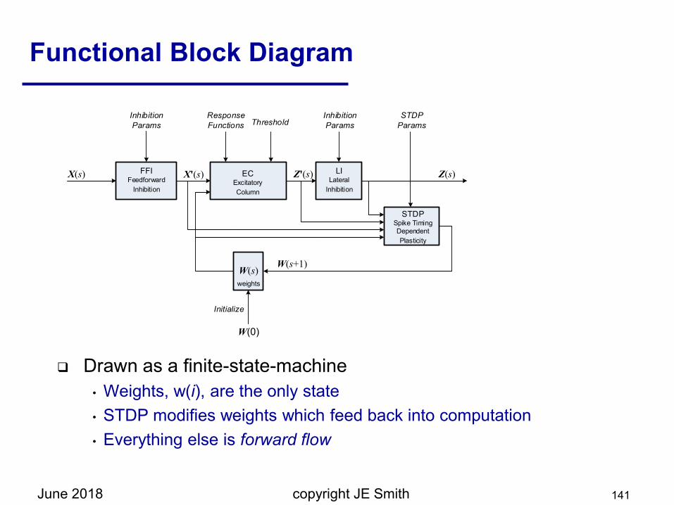
❑ Drawn as a finite-state-machine

• Weights, w(i), are the only state

• STDP modifies weights which feed back into computation

• Everything else is forward flow


X(s) ECExcitatory

Column

Response

Functions Threshold

W(s)

weights

Z'(s) Z(s)LILateral

Inhibition

STDPSpike Timing Dependent

Plasticity

W(s+1)

FFIFeedforward

Inhibition

Inhibition

Params

Inhibition

Params

W(0)

Initialize

X'(s)

STDP

Params

❑ Done on per pixel basis

❑ Compute mean of “surround”

• Currently using arithmetic mean

❑ Compare with “center” – subtract

❑ Determine center’s output spike time

Input Translation (OnOff Encoding)


❑ Example is an On-Center cell

• Convention: a lower number is

more intense input & earlier

spike

❑ Same inputs for an Off-Center cell

yields no spike

❑ On-Center and Off-Center for

same pixel never simultaneously

spike

calculate

mean

of

surround

subtract

On

center s

value3

57

7

6 7 5

4

3 5

3 2

2

❑ MNIST examples

❑ Darker pixels correspond to earlier spikes

Input Translation (OnOff Encoding)


On-Center Off-Center On-Center Off-Center

❑ If the outputs feed another TNN block, then no decoding is needed

❑ If we want to understand the outputs then we need to decode cluster Ids

• Unsupervised training (and connectivity pattern) chooses the cluster Ids

❑ Construct a small, simple output classifier (decoder)

Output Decoding


TNN1

.

.

.

Video

Input Encode

.

.

.

TNN2

.

.

.

Audio

Input Encode

.

.

.

.

.

.

.

.

.

.

.

.

TNN3

features indicative

of a small, furry

animal

features

indicative of

“meow”

...

Decode

“cat”

...

features indicative

of a cat

Unsupervised Training -- Measuring “Accuracy”

❑ A challenge because mapping from cluster identifiers to class information is opaque

❑ Add trained classifier at output to make it transparent

• For external human interpretation

• Classifier should be simple (trivial)

• Classification may be lossy

❑ Classifier results may feed back into network design process

❑ If Clustering Network is part of a larger system, outputs can be fed directly to

downstream network(s)


Test Pattern

Output PatternTrained

Clustering Network

MetaData (label)

TrainedClassifier

Compare Correct / Incorrect

training not shown

Modify Networkfeedback loop

Volley Analyzer

June 2018 146

❑ First, convert to purely spatial approximation: binary cluster identifier

❑ Note: some temporal information may be discarded

copyright JE Smith

11010011

1) Convert to binary

Decode Table

2) Cluster Identifier

indexes into

Decode Table

3) Decode Table

estimates clustering

accuracy

Decode Table

June 2018 147

❑ Use labels to associate inputs with cluster identifiers

• Assign “accuracy”

❑ Example

copyright JE Smith

label counts similarity

cluster identifier A B C D total maximum group

000011 11 34 58 0 103 58 C

000110 49 116 192 329 686 329 D

001100 41 71 426 11 549 426 C

001001 4 2 35 0 41 35 C

001010 0 6 160 7 173 160 C

011000 15 397 36 2 450 397 B

010100 0 24 2 0 26 24 B

010010 56 0 6 2 64 56 A

010001 110 0 95 45 250 110 A

110000 0 82 65 5 152 82 B

100100 1 0 1 0 2 1 C

101000 6 3 6 0 15 6 C

100001 101 58 18 62 239 101 A

2750 1785

accuracy = 0.65

Space-Time Theory and Algebra

Space-Time Computing Network


A Spacetime Computing System is a feedforward composition of functions

Fi: <x1..xq > → z ; x1..q , z {0, 1, … , }

All Fi satisfy:

computability: Fi implements a computable total function.

causality: For all xj > z, Fi (x1...,xj,...xq) = Fi (x1...,,...xq), and if z , then z ≥ xmin .

invariance: Fi(x1 + 1 .. xq + 1) = Fi(x1..xq) + 1

TNNs are Space-Time Computing Networks

.

.

.

Input

Val

ues

Encode

to

Spikes

Decode

from

Spikes

F1

F4

F5

Fn

Fn-2

F2

F3

Fn-1

.

.

.

x1

x2

xm

z2

zp

z1

26

1

37

4

9

12 60

57

7079

75

0O

utp

ut V

alues

...

...

...

...

...

...

.

.

.

.

.

.

.

.

.

Space-Time Algebra


❑ S-T Algebra

❑ Bounded Distributive Lattice

• 0, 1, 2,…,

• Ordering relation: “<”

• Interpretation: points in time

.

.

.

3

2

1

0

Top

Bottom

0

1

11

00

01 10

111

000

001 010 100

011 101 110. . .

❑ Boolean Algebra

❑ Complemented Distributive Lattice

• 0, 1 (2-valued case)

• Ordering relation: “<”

• Interpretation: logical values

Primitive S-T Operations


“atomic excitation”

“atomic inhibition”

“atomic delay”

inc: b = a + 1

a 1 b

lt: if a < b then c = a

else c =

ca

b

≺

min: if a < b then c = aelse c = b

ca

b

Space-Time Networks


❑ Theorem: Any feedforward composition of s-t functions is an s-t function

⇒ Build networks by composing s-t primitives

• Example:

note: shorthand for n increments in series:

x2

x1

y

2

x3 1

0 2

1

4 55

x46

5

a n b = a + n

Elementary Functions


❑ Increment and identity are the only one-input functions

❑ Table of all two-input s-t functions

• Many are non-commutative

function name symbol

if a < b then a; else b min

if a b then a; else not equal ≢

if a < b then a exclusive min xelse if b < a then b; else

if a > b then a; else b max

if a > b then a exclusive max xelse if b > a then b; else

if a =b then a; else equal ≡

if a b then a; else less or equal ≼

if a < b then a; else less than ≺

if a b then a; else greater or equal ≽

if a > b then a; else greater than ≻

Implementing Some Elementary Functions


greater or equal,

using lt

ack: Cristóbal Camarero

max using ge and min

equals using ge and

max

a

a

c = a b = a (a b)

b

a

b

c = a b = (a b) (b a )

a

b

a

b

a

b

c = a b = (a b) (b a )

Completeness


❑ Theorem: min, inc, and lt are functionally complete for the set of s-t functions

• equals can be implemented w/ min and lt

❑ Proof: by construction via normalized function table

• Example:

x1 x2 x3 y

0 1 2 3

1 0 2

2 2 0 2 y

x3

x1 1

x2 2

3

2

1

x1

x2

x3

0

0

2

x1

x2

x3

y

3

33

x32

x1 10

x21

2

0

3

2

1

x1

x2

x3

0

1

2

0

0

2

x1

x2

x3

0

1

2

1

4

3

3

1

3

Example


Input x1 = 0, x2 = 1, x3 = 2

x1 x2 x3 y

0 1 2 3

1 0 2

2 2 0 2

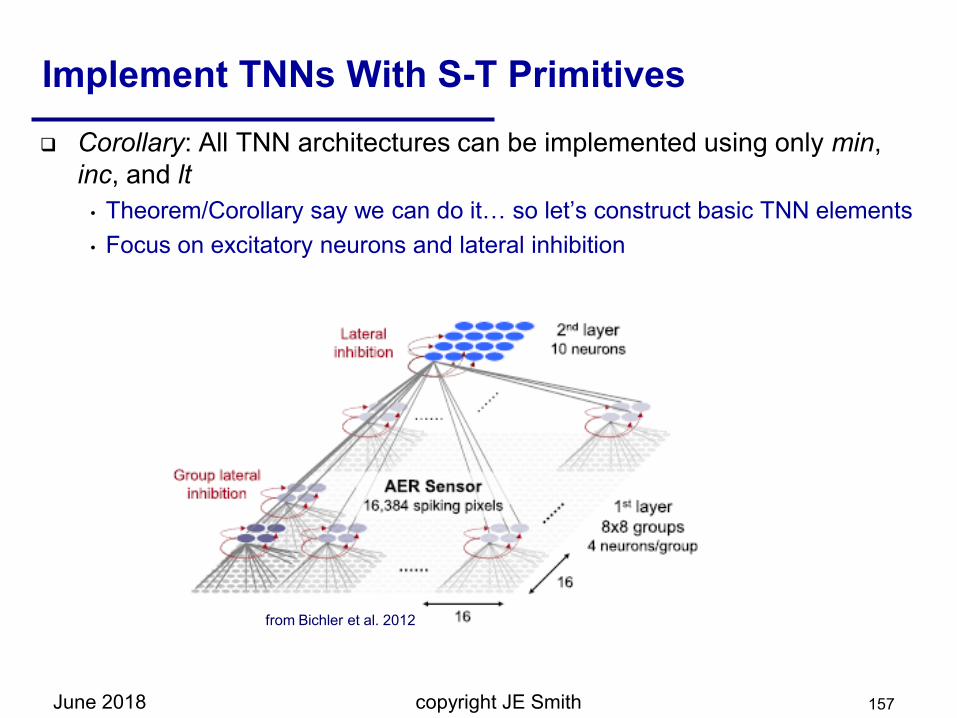
Implement TNNs With S-T Primitives


❑ Corollary: All TNN architectures can be implemented using only min,

inc, and lt

• Theorem/Corollary say we can do it… so let’s construct basic TNN elements

• Focus on excitatory neurons and lateral inhibition

from Bichler et al. 2012

Quick Review: SRM0 Neuron Model


.

.

....

response

functions

w1

w2

wp

Σ

body

potential

x2

x1

xp

y

input spikes synapses

SRM0 Neurons


❑ Start with SRM0 neurons

• A response function can be specified as up and down steps

This not a toy example – it is realistically low resolution

0 1 2 3 4 5 6 7 8 9 10 11 12

1

2

3

4

5

time

ampli

tude

x

1

1

2

2

3

7

5

8

10

12

up

steps

down

steps

x+3

x+2

x+2

x+1

x+1

x+5

x+7

x+8

x+10

x+12

Bitonic Sort (Batcher 1968)

❑ Sort is a space-time function

❑ A key component to the SRM0 construction

❑ Bitonic sorting network (Batcher) is a composition of max/min elements


x1Bitonic Sort Array

log2m (log2m+1)/2 layers

m/2 compare elts. each

x2

xm

z1

z2

zm

A

B

max(A,B)

min(A,B)

Complete SRM0 neuron


❑ Up Network: sort times of all up steps

❑ Down Network: sort times of all down

steps

❑ ≺ & min tree determines the first time no. of up steps ≥ no. of down steps +

• This is the first time the threshold is

reached

❑ Supports all possible finite response

functions

• I.e., all response functions that can

be physically implemented

• Includes inhibitory (negative)

response functions

i + -1

i

≺

.

.

.

x1

xm

Sortsmallest

to

largest

1

2

θ

θ+1

q

q-1

. . .

Up

Network

z

.

.

.

u

u

u

. . .

u

u

u

. . .

.

.

.Sort

smallest

to

largest

1

2

q - θ

q - θ +1

. . .

Down

Network

d

d

d

. . .

d

d

d

. . .

. . .

Synaptic Weights


❑ Synaptic weights determine the response function

• Synaptic weights map to /0 “micro-weights” that control network

composed of on/off lt gates and fanned-out up/down increment gates

• Hence, micro-weight switch settings determine s-t response function

di /0 μ1

x ui

diμ2

ui

diμ3

ui

diμ4

ui

ui

di0 ui -1time

di -1

am

pli

tud

e

1

2

3

4

/0

/0

/0

WTA Inhibition


❑ Winner take all inhibition

• Only the first spike in a volley is allowed to pass

• Inhibitory neurons modeled en masse

• A form of lateral inhibition

Aside: this is an example of

physical feedback, but no

functional feedback

x1 y1

xp yp

x2 y2

.

.

.

.

.

.

. . .

. . .

. . .1

.

.

.

5

7

6

5

TNN Summary


❑ We have implemented all the important functions

1) SRM0 neurons

2) Synaptic weights

3) WTA (lateral) inhibition

.

.

.

x1

xm

Sortsmallest

tolargest

1

2

+1

q

q-1

. . .

Up

Network

z

.

.

.

u

u

u

. . .

u

u

u

. . .

.

.

.Sort

smallestto

largest

1

2

q -

q – (+1)

. . .

Down

Network

d

d

d

. . .

d

d

d

. . .

min

. . .

<

<

<

<

di /0 μ1

x ui

diμ2

ui

diμ3

ui

diμ4

ui

ui

di0 ui -1time

di -1

am

plit

ude

1

2

3

4

/0

/0

/0

<

<

<

<

x1 y1

xn yn

x2 y2

min

.

.

.

.

.

.

. . .

. . .

. . .1

.

.

.

<

<

<

Implementations

Paradigms, Platforms, Implementations


❑ Paradigm

• A mathematical/algorithmic computing model

❑ Platform

• Hardware and software infrastructure upon which a paradigm is implemented

❑ Implementations

• Direct: transient events in the paradigm are implemented directly in the

hardware (e.g. voltage pulses or edges)

• Indirect: transient event timing is simulated; e.g., times are maintained and

operated on as binary encoded values

Platform Types


❑ General purpose, indirect

• Example: simulator written in Matlab running on a desktop

❑ Special purpose, indirect

• FACET

• IBM TrueNorth

• SpiNNaker

• Intel Loihi

❑ Special purpose, direct

• Analog neuromorphic, ala Carver Mead

• Generalized race logic (to follow)

[Schemmel et al. 2010]

[Merolla et al. 2011]

[Furber et al. 2014]

[Davies et al. 2018]

[Mead 1990]

My Simulator (Indirect Implementation)

Simulation Infrastructure

❑ Written in Matlab (in a block-

structured FORTRAN style)

❑ Convert input data to standard

SpikeFile form and save

❑ Thereafter, all spike information

is passed around in SpikeFile

format

❑ Simulator consists of:

• Multiple frontends (1 per layer)

• Common backend

• Intermediate data passed

through save/load SpikeFiles

❑ Network connection files are

generated separately

❑ Analysis and engineering “note

taking” is done ad hoc using

Excel as a base

June 2018 copyright JE Smith

PosNeg Filter

Generate SpikeFiles

download from MNIST website

OnOff Filter

Generate SpikeFiles

Generate

Networks

Simulator

Analysis Tools

Excel

Spreadsheets

Display

OnOff Filtered

Display MNIST

SpikeFiles

Network

Connection

files

MNIST

Benchmark

files

BackendL1

L2

LN

Frontends

(1 per layer)

Pipeline SpikeFiles

L1

L2

LN

PrintMNIST.m

GenOnOff.m

GenPosNeg.m

GenNetwork.m

FilterOnOff.m

PrintFilter.m

L1.m

pipe.m

L2.m

LN.m

L0

169

SpikeFile Format

❑ Two data arrays

• ImageList has one entry per image

pointer into SpikeList

spike count

label and other meta-data

• SpikeList contains all spikes in a

sparse vector format

❑ Matlab save/load stores and

communicates these

structures via secondary

storage


1 5 1 5

6 2 2 0

8 0 3 4

8 3 4 1

11 5 5 9

. . .

. . .

. . .

. . .

1 4

8 6

7 7

9 7

10 7

4 6

6 7

3 5

9 5

2 7

2 6

5 6

6 7

3 7

4 7

ImageList SpikeList

...

...

...

...

...

Simulator Backend Pipeline

❑ Two main stages

• 2nd larger than first

• Files saved in between

• Decomposes pipeline development

❑ Weights are the only maintained state

• Updated dynamically via STDP

❑ Several sub-stages

• MG: merge input streams

• VA: volley analyzer; computes pareto

curves for inhibition

• IC: inhibitory column

• EC: excitatory column

evaluates new inputs

applies WTA inhibition

updates weights according to STDP


VA1pareto

IC1

ECeval

ECSTDP update

VA2

inhibition params

MG

STAGE 1

STAGE 2

Data In(sparse spike format)

Control

IC2WTA-inhibition

weights

Data Out(sparse spike format)

plots and statistics

plots and statistics

Simulator Architecture


Layer 2

General Case

.

.

.

.

.

.

.

.

.

.

.

.

.

.

.

Statistics, Tables, Graphs

.

.

.

.

.

.

.

.

.

.

.

.

MGMG

Inp

ut

Pa

ttern

s

.

.

.

Layer 1

Input Special Case

.

.

.

.

.

.

input

SpikeFilespipeline

SpikeFiles

pipeline

SpikeFiles

EC ICOnOff

MG IC

EC ICOnOff

MG IC

EC ICOnOff

MG IC

EC ICIC

EC ICIC

EC ICIC

VA VA VA VA

Offline

output/input

SpikeFiles

pipeline

SpikeFiles

pipeline

SpikeFilesoutput/input

SpikeFiles

Simulator Architecture

❑ Forward flow in simulator mimics forward flow in network

❑ OnOff encoding done once on MNIST images, then saved

❑ Addressable buffers separate stages

• Connectivity established via buffer addresses

• Buffers are actually files, so stages can be simulated in different simulator runs


Layer 2

General Case

.

.

.

.

.

.

.

.

.

.

.

.

.

.

.

Statistics, Tables, Graphs

.

.

.

.

.

.

.

.

.

.

.

.

MGMG

Inp

ut

Pa

ttern

s

.

.

.

Layer 1

Input Special Case

.

.

.

.

.

.

input

SpikeFilespipeline

SpikeFiles

pipeline

SpikeFiles

EC ICOnOff

MG IC

EC ICOnOff

MG IC

EC ICOnOff

MG IC

EC ICIC

EC ICIC

EC ICIC

VA VA VA VA

Offline

output/input

SpikeFiles

pipeline

SpikeFiles

pipeline

SpikeFilesoutput/input

SpikeFiles

Direct Implementations

Classic Neuromorphic Systems

❑ The idea:

• Literally build hardware that communicates via spikes in time

• An attempt to capture efficiency benefits of spiking neurons


from Indeveri et al. 2011

❑ This is a direct implementation

• Extend to other implementations that communicate via events in time

• Edges are also events in time… ⇒ Generalized Race Logic

Race Logic: Shortest Path


❑ Shortest path computing network

• Weights implemented as shift registers

• Min functions implemented as AND gates

6

3

8

2

1

6

4

6

3

7

53

4

2

3

❑ By Madhavan et al. (2015)

6

4

6

1

3

4

2

8

5

3

7

2

3

t = 0

t = 0

t = 0

t = 2

t = 1

t = 4

t = 4

t = 7 3

6

t = 7

Network Operation

❑ Initialize all signals to 1

❑ At time t=0, transition 1→ 0 on all primary inputs

❑ Transitions sweep forward in network

• Transition times are values

❑ The time it takes to compute the short path is the short path


6

4

6

1

3

4

2

8

5

3

7

2

3

t = 0

t = 0

t = 0

t = 2

t = 1

t = 4

t = 4

t = 7 3

6

t = 7

Bitonic Sort (Batcher 1968)

❑ Sort is a space-time function

❑ A key component to the SRM0 construction

❑ Bitonic sorting network (Batcher) is a composition of max/min elements


x1Bitonic Sort Array

log2m (log2m+1)/2 layers

m/2 compare elts. each

x2

xm

z1

z2

zm

A

B

max(A,B)

min(A,B)

❑ S-T primitives implemented directly with conventional digital circuits

• Signal via 1 → 0 transitions

⇒ We can implement SRM0 neurons and WTA inhibition with off-the-shelf CMOS

⇒Very fast and efficient TNNs

Generalized Race Logic


a

bmax(a,b)OR

a a + 1D Q

ab

min(a,b)AND

ab

a ≺ b

reset

NORNOR

NOR

Exercise


❑ Build an SRM0 neuron using generalized race logic

.

.

.

x1

xm

Sortsmallest

tolargest

1

2

+1

q

q-1

. . .

Up

Network

z

.

.

.

u

u

u

. . .

u

u

u

. . .

.

.

.Sort

smallestto

largest

1

2

q -

q – (+1)

. . .

Down

Network

d

d

d

. . .

d

d

d

. . .

min

. . .

<

<

<

<

di /0 μ1

x ui

diμ2

ui

diμ3

ui

diμ4

ui

ui

di0 ui -1time

di -1

am

plit

ude

1

2

3

4

/0

/0

/0

<

<

<

<

x1 y1

xn yn

x2 y2

min

.

.

.

.

.

.

. . .

. . .

. . .1

.

.

.

<

<

<

Implication: Construct architectures in the neuroscience domain

Implement directly with off-the-shelf CMOS

ab

a < b

reset

NORNOR

NOR

ab

max(a,b)OR

ab

min(a,b)AND

a a + 1D Q

Concluding Remarks

Research Directions


❑ Huge research space

• Response functions

• Computation in dendrites

• STDP update functions

• Network connectivity patterns

• Sensory interfaces

• Hippocampus and memory

• Motor control

❑ s-t algebraic methods for implementing functions

• Look beyond TNNs

• What design methodology works? (natural,

intuitive)

❑ Study direct implementation with GRL

• Study performance/energy tradeoffs

• What is the best way to implement delays?

Macro-Columns

Lobes

Region Hierarchy

Neocortex


Model Neurons

Biological Neurons

The Box: The way we (humans) perform computation


❑ We try to eliminate temporal effects when implementing functions

• s-t uses the uniform flow of time as a key resource

❑ We use add and mult as primitives for almost all mathematical models

• Neither add nor mult is an s-t function

❑ We prefer high resolution (precision) data representations

• s-t practical only for very low-res direct implementations

❑ We strive for complete functional completeness

• s-t primitives complete only for s-t functions

• There is no inversion, complementation, or negation

❑ We strive for algorithmic, top-down design

• TNNs are based on implied functions

• Bottom-up, empirically-driven design methodology

Think outside the box!

Acknowledgements


Raquel Smith, Mikko Lipasti, Mark Hill, Margaret Martonosi, Cristobal

Camarero, Mario Nemirovsky, Mikko Lipasti, Tim Sherwood, Advait

Madhavan, Shlomo Weiss, Ido Guy, Ravi Nair, Joel Emer, Quinn

Jacobson, Abhishek Bhattacharjee

Bibliography


Ananthanarayanan et al. 2009: R. Ananthanarayanan, S. K. Esser, H. D. Simon, and D. S. Modha, "The cat is out of the bag: cortical simulations

with 109 neurons, 1013 synapses." High Performance Computing Networking, Storage and Analysis, 2009.

Arthur et al. 2012: Arthur, J.V., Merolla, P.A., Akopyan, F., Alvarez, R., Cassidy, A., Chandra, S., Esser, S.K., Imam, N., Risk, W., Rubin, D.B. and

Manohar, R., “Building block of a programmable neuromorphic substrate: A digital neurosynaptic core,” 2012 International Joint Conference on Neural

Networks, pp. 1-8, 2012.

Bakkum et al. 2008: Bakkum, Douglas J., Zenas C. Chao, and Steve M. Potter, “Long-term activity-dependent plasticity of action potential

propagation delay and amplitude in cortical networks”, PLOS one 3.5 (2008): e2088.

Batcher 1968: Batcher, K. E., “Sorting networks and their applications,” Proceedings of the Spring Joint Computer Conference, pp. 307-314, 1968.

Beyeler et al. 2013: Beyeler, Michael, Nikil D. Dutt, and Jeffrey L. Krichmar. "Categorization and decision-making in a neurobiologically plausible

spiking network using a STDP-like learning rule." Neural Networks 48 (2013): 109-124.

Bi and Poo 1998: Bi, G.-Q., and M.-M. Poo, “Synaptic modifications in cultured hippocampal neurons: dependence on spike timing, synaptic

strength, and postsynaptic cell type,” The Journal of Neuroscience 18, no. 24, pp. 10464-10472, 1998.

Bichler et al. 2012: Bichler, O., D. Querlioz, S. J. Thorpe, J.-P. Bourgoin, and C. Gamrat, “Extraction of temporally correlated features from dynamic

vision sensors with spike-timing-dependent plasticity,” Neural Networks 32, pp. 339-348, 2012.

Bohte et al. 2002a: Bohte, S. M., H. La Poutré, and J. N. Kok, “Unsupervised clustering with spiking neurons by sparse temporal coding and

multilayer RBF networks,” IEEE Transactions on Neural Networks, 13, no. 2, pp. 426-435, 2002.

Bohte et al. 2002b: Bohte, S. M., J. N. Kok, and H. La Poutré, “Error-backpropagation in temporally encoded networks of spiking neurons,”

Neurocomputing 48, no. 1 pp.17-37, 2002.

Brader et al. 2007: Brader, Joseph M., Walter Senn, and Stefano Fusi. "Learning real-world stimuli in a neural network with spike-driven synaptic

dynamics." Neural computation 19, no. 11 (2007): 2881-2912.

Brette 2015: Brette, R., “Philosophy of the spike: rate-based vs. spike-based theories of the brain,” Frontiers in Systems Neuroscience 9, 2015.

Bibliography


Carlo and Stevens 2013: Carlo, C. Nikoosh, and Charles F. Stevens. "Structural uniformity of neocortex, revisited." Proceedings of the

National Academy of Sciences 110, no. 4 (2013): 1488-1493.

Davies et al. 2018: Davies, Mike, Narayan Srinivasa, Tsung-Han Lin, Gautham Chinya, Yongqiang Cao, Sri Harsha Choday, Georgios

Dimou et al. "Loihi: A neuromorphic manycore processor with on-chip learning." IEEE Micro 38, no. 1 (2018): 82-99.

DeFelipe et al. 2002: DeFelipe, Javier, Lidia Alonso-Nanclares, and Jon I. Arellano. "Microstructure of the neocortex: comparative aspects."

Journal of neurocytology 31, no. 3-5 (2002): 299-316.

DeFelipe 2011: DeFelipe, Javier. "The evolution of the brain, the human nature of cortical circuits, and intellectual creativity." Frontiers in

neuroanatomy 5 (2011).

Delorme et al. 1999: Delorme, A., J. Gautrais, R. van Rullen, and S. Thorpe, “SpikeNet: A simulator for modeling large networks of integrate

and fire neurons,” Neurocomputing, 26-27, pp. 989-996, 1999.

DeLorme et al. 2001: Delorme, Arnaud, Laurent Perrinet, and Simon J. Thorpe, Networks of Integrate-and-Fire Neurons using Rank Order

Coding B: Spike Timing Dependant Plasticity and Emergence of Orientation Selectivity Neurocomputing 38 (2001): 539-545.

Diehl et al. 2015: Diehl, P. U., D. Neil, J. Binas, M. Cook, S.-C. Liu, and M. Pfeiffer, “Fast-classifying, high-accuracy spiking deep networks

through weight and threshold balancing,” 2015 International Joint Conference on Neural Networks, pp. 1-8, 2015.

Deiss et al. 1999: Deiss, S. R., R. J. Douglas, and A. M. Whatley, “A pulse-coded communications infrastructure for neuromorphic systems,”

Pulsed Neural Networks , pp. 157-178, 1999.

Eliasmith et al. 2012: Eliasmith, C., T. C. Stewart, X. Choo, T. Bekolay, T. DeWolf, C. Tang, and D. Rasmussen, “A large-scale model of the

functioning brain,” Science 338, no. 6111, pp.1202-1205, 2012.

Fauth et al. 2015: Fauth, Michael, Florentin Wörgötter, and Christian Tetzlaff. "The Formation of Multi-synaptic Connections by the

Interaction of Synaptic and Structural Plasticity and Their Functional Consequences." PLoS computational biology 11, no. 1 (2015).

Felleman and Van Essen 1991: Felleman, Daniel J., and David C. Van Essen. "Distributed hierarchical processing in the primate cerebral

cortex." Cerebral cortex 1, no. 1 (1991): 1-47.

Bibliography


Fries et al. 2007: Fries, P., D. Nikolić, and W. Singer, “The gamma cycle,” Trends in Neurosciences 30, no. 7 pp. 309-316, 2007.

Furber et al. 2014: Furber, Steve B., Francesco Galluppi, Steve Temple, and Luis A. Plana. "The spinnaker project." Proceedings of the IEEE

102, no. 5 (2014): 652-665.

Fusi and Mattia 1998: Fusi, S., and M. Mattia, “Collective behavior of networks with linear (VLSI) integrate-and-fire neurons,” Neural

Computation 11.3, pp. 633-652, 1998.

Gerstner et al. 1996: Gerstner, W., R. Kempter, J. L. van Hemmen, and H. Wagner, “A neuronal learning rule for sub-millisecond temporal

coding,” Nature 383, no. 6595, pp. 76-78, 1996.

Gütig and Haim 2006: Gütig, R., and Haim S., “The tempotron: a neuron that learns spike timing–based decisions,” Nature Neuroscience 9,

no. 3, pp. 420-428, 2006.

Gütig et al. 2013: Gütig, R., Tim G., H. Sompolinsky, and M. Meister, “Computing complex visual features with retinal spike times,” PloS One

8, no. 1, e53063, 2013.

Guyonneau et al. 2004: Guyonneau, R., R. VanRullen, and S. J. Thorpe, “Temporal codes and sparse representations: A key to

understanding rapid processing in the visual system,” Journal of Physiology-Paris 98, pp. 487-497, 2004.

Guyonneau et al. 2005: Guyonneau, R., R. VanRullen, and S. J. Thorpe, “Neurons tune to the earliest spikes through STDP,” Neural

Computation 17, no. 4, pp. 859-879, 2005.

Hawkins and Blakeslee 2007: Hawkins, J., and S. Blakeslee. On intelligence: How a new understanding of the brain will lead to the creation

of truly intelligent machines. Macmillan, 2007.

Hill et al. 2012: Hill, Sean L., et al., Statistical connectivity provides a sufficient foundation for specific functional connectivity in neocortical

neural microcircuits, Proceedings of the National Academy of Sciences (2012).

Hodgkin and Huxley 1952: Hodgkin, Alan L., and Andrew F. Huxley, A Quantitative Description of Membrane Current and Its Application to

Conduction and Excitation in Nerve -- The Journal of physiology 117.4 (1952): 500.

Bibliography


Hopfield 1995: Hopfield, J. J., “Pattern recognition computation using action potential timing for stimulus representation,” Nature 376, pp. 33-

36, 1995.

Indiveri et al. 2011: Indiveri, G., Linares-Barranco, B., Hamilton, T.J., Van Schaik, A., Etienne-Cummings, R., Delbruck, T., Liu, S.C., Dudek,

P., Häfliger, P., Renaud, S. and Schemmel, J., “Neuromorphic silicon neuron circuits”, Frontiers in Neuroscience 5, 2011.

Irwin and Shen 2005: Irwin, M. J., and J. P. Shen, “Revitalizing computer architecture research,” Computing Research Association, 2005.

Izhikevich and Edelman 2008: Izhikevich, Eugene M., and Gerald M. Edelman Large-scale model of mammalian thalamocortical systems,

Proceedings of the national academy of sciences 105.9 (2008): 3593-3598. Also: Supporting Information

Izhikevich et al. 2004: Izhikevich, Eugene M., Joseph A. Gally, and Gerald M. Edelman, “Spike-timing dynamics of neuronal groups”,

Cerebral Cortex 14.8 (2004): 933-944.

Karnani et al. 2014: Karnani, M. M., M. Agetsuma, and R. Yuste, “A blanket of inhibition: functional inferences from dense inhibitory

connectivity,” Current opinion in Neurobiology 26, pp. 96-102, 2014.

Kermany et al. 2010: Kermany, Einat, et al., Tradeoffs and Constraints on Neural Representation in Networks of Cortical Neurons –The

Journal of Neuroscience 30.28 (2010): 9588-9596.

Kheradpisheh et al. 2016a: Kheradpisheh, S. R., M. Ganjtabesh, and T. Masquelier, “Bio-inspired unsupervised learning of visual features

leads to robust invariant object recognition,” Neurocomputing 205, pp. 382-392, 2016.

Kheradpisheh et al. 2016b: Kheradpisheh, S. R., M. Ganjtabesh, S. J. Thorpe, and T. Masquelier, “STDP-based spiking deep neural

networks for object recognition,” arXiv preprint arXiv:1611.01421, 2016.

Kistler et al. 1997: Kistler, W. M., W. Gerstner, and J. L. van Hemmen, “Reduction of the Hodgkin-Huxley equations to a single-variable

threshold model”, Neural Computation 9.5, pp. 1015-1045, 1997.

Körner et al. 1999: Körner, Edgar, M-O. Gewaltig, Ursula Körner, Andreas Richter, and Tobias Rodemann. "A model of computation in

neocortical architecture." Neural Networks 12, no. 7 (1999): 989-1005.

Bibliography


Laurent 1999: Laurent, Gilles. "A systems perspective on early olfactory coding." Science 286, no. 5440 (1999): 723-728.

LeCun et al. 2015: LeCun, Y., Y. Bengio, and G. Hinton, “Deep learning,” Nature 521, no. 7553, pp. 436-444, 2015.

Lee et al. 2010: Lee, Jungah, HyungGoo R. Kim, and Choongkil Lee. "Trial-to-trial variability of spike response of V1 and saccadic response

time." Journal of neurophysiology 104, no. 5 (2010): 2556-2572.

Lennie 2003: Lennie, Peter. "The cost of cortical computation." Current biology 13, no. 6 (2003): 493-497.

Lippmann 1987: Lippmann, Richard, “An introduction to computing with neural nets” , ASSP Magazine, pp. 4-22, 1987.

Madhavan et al. 2015: Madhavan, A., T. Sherwood, and D. Strukov, “Race logic: abusing hardware race conditions to perform useful

computation,” IEEE Micro 35, no. 3, pp. 48-57, 2015.

Maass 1995: Maass, W., “On the computational complexity of networks of spiking neurons” (extended abstract), Advances in Neural

Information Processing Systems, vol. 7, p. 183, 1995.

Maass 1997: Maass, W., “Networks of spiking neurons: the third generation of neural network models,” Neural Networks 10.9, pp.1659-1671,

1997.

Maass 1999: Maass, W. Computing with Spiking Neurons, In Pulsed Neural Networks, W. Maass and C. M. Bishop, editors, pages 55-85.

MIT Press (Cambridge), 1999.

Mainen and Sejnowski 1995: Mainen, Z. F., and T. J. Sejnowski, "Reliability of spike timing in neocortical neurons,” Science 268, no. 5216 ,

pp. 1503-1506, 1995.

Markram et al. 1997: Markram, H., J. Lübke, M. Frotscher, and B. Sakmann, “Regulation of synaptic efficacy by coincidence of postsynaptic

APs and EPSPs,” Science 275, no. 5297, pp. 213-215, 1997.

Markram et al. 2004: Markram, Henry, Maria Toledo-Rodriguez, Yun Wang, Anirudh Gupta, Gilad Silberberg, and Caizhi Wu. "Interneurons

of the neocortical inhibitory system." Nature Reviews Neuroscience 5, no. 10 (2004): 793-807.

Bibliography


Masquelier and Thorpe 2010: Masquelier, T., and S. J. Thorpe, “Learning to recognize objects using waves of spikes and Spike Timing-

Dependent Plasticity,” 2010 International Joint Conference on Neural Networks, pp. 1-8, 2010.

Masquelier and Thorpe 2007: Masquelier, T., and S. J. Thorpe, “Unsupervised learning of visual features through spike timing dependent

plasticity,“ PLoS Comput Biol 3, no. 2, e31, 2007.

McKennoch et al. 2006: McKennoch, S., D. Liu, and L. G. Bushnell, “Fast modifications of the spikeprop algorithm,” International Joint

Conference on Neural Networks, pp. 3970-3977, 2006.

Mead 1990: Mead, Carver. "Neuromorphic electronic systems." Proceedings of the IEEE 78, no. 10 (1990): 1629-1636.

Merolla et al. 2011: Merolla, Paul, John Arthur, Filipp Akopyan, Nabil Imam, Rajit Manohar, and Dharmendra S. Modha. "A digital

neurosynaptic core using embedded crossbar memory with 45pJ per spike in 45nm." In 2011 IEEE custom integrated circuits conference

(CICC), pp. 1-4. IEEE, 2011.

Morrison et al. 2008: Morrison, A., M. Diesmann, and W. Gerstner, “Phenomenological models of synaptic plasticity based on spike timing,”

Biological Cybernetics 98, no. 6, pp. 459-478, 2008.

Mountcastle 1997: Mountcastle, V., “The Columnar organization of the neocortex,” Brain 120, no. 4, pp. 701-722, 1997.

NAE: NAE Grand Challenges for Engineering, “Reverse Engineer the Brain”, http://www.engineeringchallenges.org/challenges/9109.aspx

Natschläger and Ruf 1998: Natschläger, T., and B. Ruf, “Spatial and temporal pattern analysis via spiking neurons,” Network: Computation

in Neural Systems 9, no. 3, pp. 319-332, 1998.

Natschläger and Ruf 1999: Natschläger,., and B. Ruf, “Pattern analysis with spiking neurons using delay coding,” Neurocomputing 26, pp.

463-469, 1999.

Oberlander, et al. 2012: Oberlaender, Marcel, et al. "Cell Type–Specific Three-Dimensional Structure of Thalamocortical Circuits in a

Column of Rat Vibrissal Cortex." Cerebral Cortex 22.10 (2012): 2375-2391.

O’Connor et al. 2013: O’Connor, P., D. Neil, S.-C. Liu, T. Delbruck, and M. Pfeiffer, “Real-time classification and sensor fusion with a spiking

deep belief network,” Frontiers in Neuroscience 7, 2013.

Bibliography


Perea et al. 2009: Perea, Gertrudis, Marta Navarrete, and Alfonso Araque. "Tripartite synapses: astrocytes process and control synaptic

information." Trends in neurosciences 32, no. 8 (2009): 421-431.

Perin et al. 2011: Perin, Rodrigo, Thomas K. Berger, and Henry Markram. "A synaptic organizing principle for cortical neuronal groups "

Proceedings of the National Academy of Sciences 108, no. 13 (2011): 5419-5424. – 2011.

Petersen et al. 2001: Petersen, Rasmus S., Stefano Panzeri, and Mathew E. Diamond, Population Coding of Stimulus Location in Rat

Somatosensory Cortex -- Neuron 32.3 (2001): 503-514.

Pfeil et al. 2012: Pfeil, T., T. C. Potjans, S. Schrader, W. Potjans, J. Schemmel, M. Diesmann, and K. Meier, “Is a 4-bit synaptic weight

resolution enough?–constraints on enabling spike-timing dependent plasticity in neuromorphic hardware,” Frontiers in Neuroscience 6, 2012.

Probst et al. 2012: Probst, Dimitri, et al. ,”Liquid Computing in a Simplified Model of Cortical Layer IV: Learning to Balance a Ball”, Artificial

Neural Networks and Machine Learning–ICANN 2012 (2012): 209-216.

Querlioz et al. 2013: Querlioz, D., O. Bichler, P. Dollfus, and C. Gamrat, “Immunity to device variations in a spiking neural network with

memristive nanodevices,” IEEE Transactions on Nanotechnology 12, no. 3, pp. 288-295, 2013.

Rauch et al. 2003: Rauch, A., G. La Camera, H. R. Luscher, W. Senn, and S. Fusi, “Neocortical pyramidal cells respond as integrate-and-fire

neurons to in vivo-like input currents,” Journal of Neurophysiology 90, no. 3, pp. 1598-1612, 2003.

Rinkus, 2010: Rinkus, Gerard J. "A cortical sparse distributed coding model linking mini-and macrocolumn-scale functionality." Frontiers in

Neuroanatomy 4 (2010): 17.

Salakhutdinov et al. 2007: Salakhutdinov, R., A. Mnih, and G. Hinton, “Restricted Boltzmann machines for collaborative filtering,” 24th

International Conference on Machine Learning, pp. 791-798, 2007.

Schemmel et al. 2010: Schemmel, Johannes, D. Bruderle, A. Grubl, Matthias Hock, Karlheinz Meier, and Sebastian Millner. "A wafer-scale

neuromorphic hardware system for large-scale neural modeling." In Circuits and Systems (ISCAS), Proceedings of 2010 IEEE International

Symposium on, pp. 1947-1950. IEEE, 2010.

Schrauwen and Van Campenhout 2004: Schrauwen, B., and J. Van Campenhout, “Extending spikeprop,” IEEE International Joint

Conference on Neural Networks, pp. 471-475, 2004.

Bibliography


Singer 2010: Singer, W., “Neocortical rhythms,” Dynamic Coordination in the Brain: From Neurons to Mind, eds. Von der Malsburg,

Christoph, William A. Phillips, and Wolf Singer. MIT Press, 2010.

Smith 2014: Smith, James E. "Efficient digital neurons for large scale cortical architectures." In ACM SIGARCH Computer Architecture News,

vol. 42, no. 3, pp. 229-240. IEEE Press, 2014.

Stein 1965: Stein, R. B. “A theoretical analysis of neuronal variability,” Biophysical Journal 5.2, pp. 173-194, 1965.

Thorpe and Imbert 1989: Thorpe, S. J., and M. Imbert, “Biological constraints on connectionist modelling,” Connectionism in Perspective,

pp. 63-92, 1989.

Thorpe et al. 2001: Thorpe, S., A. Delorme, and R. Van Rullen, “Spike-based strategies for rapid processing,” Neural Networks 14.6-7, pp.

715-725, 2001.

Tryon 1962: J. C. Tryon, "Quadded logic" in Redundancy Techniques for Computing Systems, Washington, DC:Spartan, pp. 205-228, 1962.

Tuckwell 1979: Tuckwell, H. C. “Synaptic transmission in a model for stochastic neural activity,” Journal of Theoretical Biology 77.1, pp. 65-

81, 1979.

Weidenbacher and Neumann 2008: Weidenbacher, U., and H. Neumann, “Unsupervised learning of head pose through spike-timing

dependent plasticity,” in Perception in Multimodal Dialogue Systems, ser, Lecture Notes in Computer Science. Springer Berlin 1 Heidelberg,

vol. 5078/2008, pp. 123-131, 2008.

VanRullen et al. 2005: VanRullen, R., R. Guyonneau, and S. J. Thorpe, “Spike Times Make Sense”, Trends in neurosciences 28.1, pp. 1-4,

2005.

Wysoski et al. 2010: Wysoski, S. G., L. Benuskova, and N. Kasabov,”Evolving spiking neural networks for audiovisual information

processing,” Neural Networks 23, pp. 819-835, 2010.

Yuste 2015: Yuste, R., “From the neuron doctrine to neural networks,” Nature Reviews Neuroscience 16, no. 8, pp. 487-497, 2015.

Zhao et al. 2015: Zhao, B., R. Ding, S. Chen, B. Linares-Barranco, and H. Tang, “Feedforward categorization on AER motion events using

cortex-like features in a spiking neural network,” IEEE Transactions on Neural Networks and Learning Systems 26, no. 9, pp. 1963-1978,

2015.

reverse-engineering the brain: a computer …...reverse-engineering the brain: a computer...

Documents

Bibliography

June 2018 copyright JE Smith 185
June 2018 copyright JE Smith 186
June 2018 copyright JE Smith 187
June 2018 copyright JE Smith 188
June 2018 copyright JE Smith 189
June 2018 copyright JE Smith 190
June 2018 copyright JE Smith 191
June 2018 copyright JE Smith 192