review article level set methods and …alma/files/tsaiosher03.pdflevel set methods and their...

COMM. MATH. SCI. c© 2003 International Press

Vol. 1, No. 4, pp. 623–656

REVIEW ARTICLE

LEVEL SET METHODS AND THEIR APPLICATIONS IN IMAGESCIENCE∗

RICHARD TSAI † AND STANLEY OSHER ‡

In this article, we discuss the question “What Level Set Methods can do for imagescience”. We examine the scope of these techniques in image science, in particularin image segmentation, and introduce some relevant level set techniques that arepotentially useful for this class of applications. We will show that image sciencedemands multi-disciplinary knowledge and flexible but still robust methods. That iswhy the Level Set Method has become a thriving technique in this field.

We begin by reviewing some typical PDE based applications in image processing.In typical PDE methods, images are assumed to be continuous functions sampled ona grid. We will show that these methods all share a common feature, which is theemphasis on processing the level lines of the underlying image. The importance of levellines has been known for some time. See e.g., [2]. This feature places our slightlygeneral definition of the level set method for image science in context. In sectiontwo, we describe the building blocks of a typical level set method in the continuumsetting. Each important task that one needs to do is formulated as the solutionto certain PDEs. Then, in section three, we quickly describe the finite differencemethods developed to construct approximate solutions to these PDEs. In section four,we discuss the Chan-Vese segmentation algorithm and two new fast implementationmethods. Finally, in section five, we describe some new techniques developed in thelevel set community as our prospectus for the future.

1. Level Set Methods and Image ScienceThe level set method for capturing moving fronts was introduced by Osher and

Sethian [72] in 1987. (Two earlier conference papers which contained some of the keyideas, have recently come to light [28, 29]). Over the years, the method has proven tobe a robust numerical device for this purpose in a diverse collection of problems. Oneset of problems lies in the field of image science. In this article, we will emphasizenot only what has been done in image science using level set techniques, but alsoin other area of sciences in which the level set methods are applied successfully —the idea is to point out the related formulations and solution methods to the imagescience communities. These communities include image/video processing, computervision, and graphics. These are diverse, with specialties such as medical imaging andHollywood type special effects.

Let us begin with a quick examination of what constitutes a classical level setmethod: an implicit data representation of a hypersurface (codimension 1 object),a set of PDEs that govern how the surface moves, and the corresponding numericalmethods for implementing this on computers. In fact, a typical application in image

∗Received: October 28, 2003; accepted (in revised version): November 5, 2003.†Institute for Advanced Study, Einstein Drive Simonyi Hall Princeton, NJ 08540, (yt-

[email protected]).‡University of California, Los Angeles, CA 90095-1555, ([email protected]).

623

624 LEVEL SET METHODS AND THEIR APPLICATIONS IN IMAGE SCIENCE

science may very well need all these features. We will illustrate this point by someclassical applications.

The term “image science” (or “imaging science”) is used here to denote a widerange of problems related to digital images. It is generally referred to problems re-lated to image processing, computer graphics, and computer vision. The type ofmathematical techniques involved range from discrete math, linear algebra, statistics,approximation theory, to partial differential equations, quasi-convexity analysis re-lated to solving inverse problems, and even algebraic geometry. The role of a level setmethod for image processing often relates to PDE techniques involving one or moreof the following features: 0) regarding an image as a function sampled on a givengrid with the grid values corresponding to the pixel intensity in suitable color space,1) regularization of the solutions, 2) representing boundaries, and 3) the numericsdeveloped for the level set methods. Particularly in light of 2), it is not hard to seekan application of the level set method for segmentation. There are, however, effortswhich combine different disciplines mentioned above together to accomplish specialtasks. For example, Mark Green [47] used a new statistical approach together withTotal Variation (TV) denoising [80], and Yves Meyer [62] analyzed function/imagerepresentation from a decomposition that is motivated by the TV denoising of [80].We will see soon that TV denoising is closely related to solving an inverse problem.

In a later section, we will examine some essential fundamentals of the level setmethodology. We refer the reader to the original paper [72] and the new book [68] fordetailed exposition of the level set method. Also, there is a set of presentation slidesavailable from the first author’s home page1.

We write a typical PDE method as

Lu = λRu,

or

ut + Lu = λRu,

where L is some operator applied to the given image, and R denotes the regularizationoperator. Typically, an image model is obtained by devising an energy functional E(u)and solving for a minimizer. The Mumford-Shah multiscale segmentation model isdefined this way [63], as is TV denoising which can be written as:

minimumuE(u) =12

∫(u− u0)2dx + λ

∫|∇u|dx,

where u0 is the given noisy image. In this set up, Lu will be the Euler-Lagrangeequation subject to the associated natural boundary conditions, which is just u −u0 here and Ru = ∇ · ∇u

|∇u| , the curvature of the level curve at each point in thisapplication. When L is not invertible, or when certain regularity in the image u isrequired, a regularization term will be added. For example, in the TV deblurring of[79],

Lu = K ∗ (Ku− u0),

1http://www.math.princeton.edu/˜ytsai

RICHARD TSAI AND STANLEY OSHER 625

where K is a compact integral operator , u0 is the given image, and the restored imageis the limit u(t) as t −→ ∞. In the usual version of Total Variation based methods,the regularization is defined as

Ru =(∇ · ∇u

|∇u|). (1.1)

This is the Euler-Lagrange derivative of the TV term as remarked above. Note thatin many image applications, the unregularized energy functional is nonconvex, andits global minimizer corresponds to the trivial solution. Only some local minimizer isneeded.

In the development of this type of method, one often qualitatively studies thesolutions of the governing PDEs by investigating what action occurs on each of thelevel sets of a given image. In the TV regularization of [61] for example, Ru(x)actually denotes the mean curvature of the level set of u passing through x. References[14, 20, 38], for example, provided analysis for these types of PDEs.

The effects of (1.1) in noise removal can be explained as follows: the level curvesin the neighborhoods of noise on the image have high curvatures. The level curves ofthe viscosity solution to

ut =(∇ · ∇u

|∇u|)|∇u|

shrink with the speed of the mean curvature and eventually disappear. Consequently,the level curves with very high curvatures (noise) disappear much faster than thosewith relatively lower curvatures, (this was the approach taken in [61]). If the |∇u|term is dropped (as it usually is) the velocity is also inversely in proportion to thegradient. This means relatively flat edges do not disappear. The analysis of motionby curvature and other geometric motions are all important consequences of viscositysolution theory, originally devised for Hamilton-Jacobi Equations, related to evolutionpast the singularities, including the pinching-off of level curves. See [20, 26, 38, 39,40, 42].

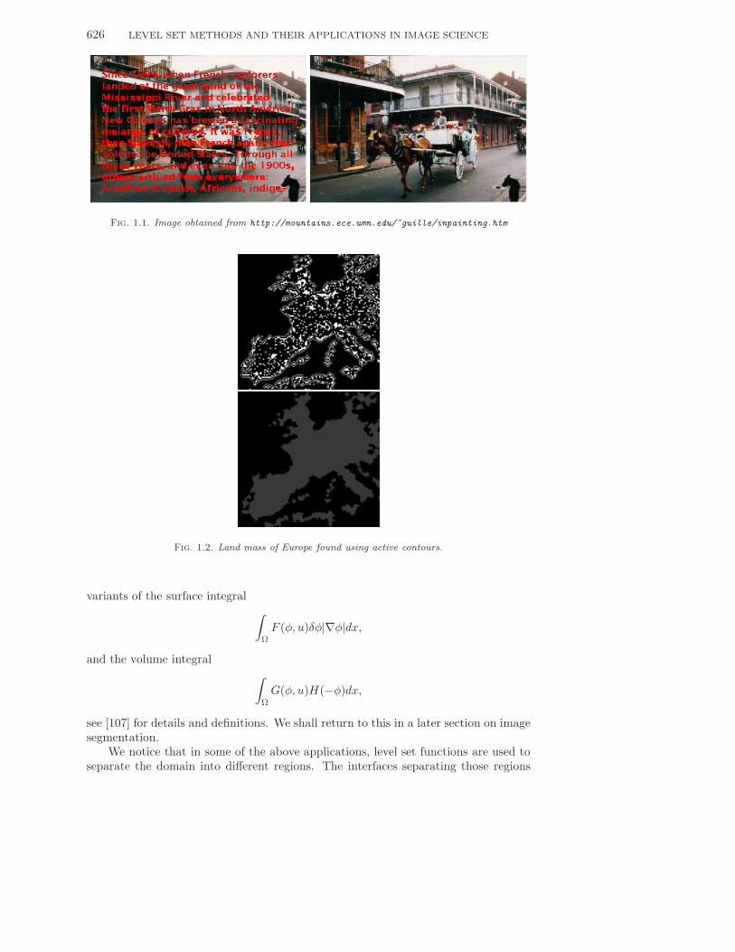
Another interesting category of applications is data interpolation. In the problemof inpainting, see e.g. [5] and Figure 1.1, the challenge is to repair images withregions of missing information. The algorithms are developed with strong motivationon connecting the level curves over the “inpainting domain” in an “appropriate way”.In a rather orthogonal way, the AMLE (Absolutely Minimizing Lipschitz Extension)algorithm, see e.g. [13], assumes a given set of level curves of an image, and fills inthe regions in between the given level curves while trying to minimize the variationof the new data generated.

In many applications such as image segmentation or rendering, level set methodsare used to define the objects of interest. For example, a level set function is usedto single out desired objects such as the land mass of Europe [18]. The land mass isdefined to be the connected region where the level set function is of one sign (see Figure1.2). There are many successful algorithms. Examples are [17, 75]. In a different, butrelated, context, Zhao et al. use a level set function to interpret unorganized datasets [108, 105].

Many of the above methods rely on the variational level set calculus similar tothat of [107] to formulate the energies whose minimizers are interpreted as the solutionto the problems, and the solutions are level set functions. In general, the energies are


Fig. 1.1. Image obtained from http://mountains.ece.umn.edu/~guille/inpainting.htm

Fig. 1.2. Land mass of Europe found using active contours.

variants of the surface integral∫

Ω

F (φ, u)δφ|∇φ|dx,

and the volume integral∫

Ω

G(φ, u)H(−φ)dx,

see [107] for details and definitions. We shall return to this in a later section on imagesegmentation.

We notice that in some of the above applications, level set functions are used toseparate the domain into different regions. The interfaces separating those regions


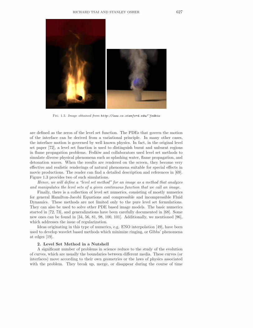
Fig. 1.3. Image obtained from http://www.cs.stanford.edu/~fedkiw

are defined as the zeros of the level set function. The PDEs that govern the motionof the interface can be derived from a variational principle. In many other cases,the interface motion is governed by well known physics. In fact, in the original levelset paper [72], a level set function is used to distinguish burnt and unburnt regionsin flame propagation problems. Fedkiw and collaborators used level set methods tosimulate diverse physical phenomena such as splashing water, flame propagation, anddetonation waves. When the results are rendered on the screen, they become veryeffective and realistic renderings of natural phenomena suitable for special effects inmovie productions. The reader can find a detailed description and references in [69].Figure 1.3 provides two of such simulations.

Hence, we will define a “level set method” for an image as a method that analyzesand manipulates the level sets of a given continuous function that we call an image.

Finally, there is a collection of level set numerics, consisting of mostly numericsfor general Hamilton-Jacobi Equations and compressible and incompressible FluidDynamics. These methods are not limited only to the pure level set formulations.They can also be used to solve other PDE based image models. The basic numericsstarted in [72, 73], and generalizations have been carefully documented in [68]. Somenew ones can be found in [34, 56, 81, 98, 100, 101]. Additionally, we mentioned [96],which addresses the issue of regularization.

Ideas originating in this type of numerics, e.g. ENO interpolation [49], have beenused to develop wavelet based methods which minimize ringing, or Gibbs’ phenomenaat edges [19].

2. Level Set Method in a NutshellA significant number of problems in science reduce to the study of the evolution

of curves, which are usually the boundaries between different media. These curves (orinterfaces) move according to their own geometries or the laws of physics associatedwith the problem. They break up, merge, or disappear during the course of time


evolution. These are the every day challenges of most of the conventional methods.The level set method [72], however, handles these topological changes in the curves“with no emotional involvement”. Since its first introduction, there has developed apowerful level set calculus used to solve a great variety of problems in fluid dynamics,materials sciences, computer vision, and computer graphics, to name a few topics.We refer to [68] for an extensive exposition of the level set calculus. See also [45] forrelated theoretical exposition.

Typically, one can write a general level set algorithm in three steps enumeratedbelow:

1. Initialize/reinitialize φ at t = tn.2. Construct/approximate H(t, x, φ,Dφ,D2φ). (Occasionally higher derivatives

also appear for which viscosity solution theory does not apply).3. Evolve

φt +H(t, x, φ,Dφ,D2φ) = 0,

for t = tn + ∆t.For image applications, φ above can either be the image itself (e.g. deblurring applica-tions) or an extra function that is used to process the given image (e.g. segmentationapplications).

We will discuss the key components of the three steps in the following sections.More precisely, we will follow a conventional approach of describing the level setmethod and start our exposition for Step 2. Step 1 and Step 3 is typically implementedby suitable numerical methods that will be reviewed in the next section.

2.1. Basic formulation. For simplicity, we discuss the conventional level setformulation in two dimensions. The interface represented by a level set function isthus also referred to as a curve. However, the methodology presented in this sectioncan be naturally extended to any number of space dimensions. There, the interfacethat is represented is generally called a hypersurface (in three dimensions, it is simplycalled a surface). We will use the words interface and curves, interchangeably.

In the level set method, the curves are implicitly defined as the zeros of a Lipschitzcontinuous function φ. This is to say that (x, y) ∈ R

2 : φ(x, y) = 0 corresponds tothe location of the embedded curve. See Figures 2.1, 2.2, and 2.3 for some examples.If we associate a continuous velocity field v whose restriction onto the curve representsthe velocity of the curve, then at least locally in time, the evolution can be describedas the Cauchy problem

φt + v · ∇φ = 0, φ(x, 0) = φ0(x),

where φ0 embeds the initial position of the curve. To derive this, let us look at aparameterized curve γ(s, t) and assume that ∂γ/∂t is the known dynamic of this curve.If we require that γ(s, t) be the zero of the function φ for all time, i.e. φ(γ(s, t), t) = 0for all t ≥ 0, then at least formally, the following equation

φt +∂γ

∂t· ∇φ(γ, t) = 0

is satisfied along γ. Extending ∂γ/∂t continuously to the whole domain will createsuch a velocity field.

In general, the velocity v can be a function of position x and some other geomet-rical quantities of the curve or other physical quantities that come with the problem.


−0.6 −0.4 −0.2 0 0.2 0.4 0.6

−0.6

−0.4

−0.2

0

0.2

0.4

0.6

Fig. 2.1. A circle embedded by different continuous functions.

The equation can be written using the normal velocity:

vn = v · ∇u|∇u| , φt + vn|∇φ| = 0. (2.1)

We note that these equations are usually fully nonlinear first order Hamilton-Jacobior second order degenerate parabolic equations, and with suitable restrictions, thetheory of viscosity solutions [25] can be applied to guarantee well-posedness of theCauchy problem.

Corresponding to the viscosity solution theory, there is a set of simple finitedifference methods to construct approximation solutions. We refer the interestedreaders to [41, 45].

Finally, in the level set formulation, the surface integral of function f along thezero level set is defined via the surface integral

∫Rd

f(x)δ(φ)|∇φ|dx.

If f ≡ 1, this integral yields the arclength for curves in two dimensions, and surface


−1 −0.8 −0.6 −0.4 −0.2 0 0.2 0.4 0.6 0.8 1−1

−0.8

−0.6

−0.4

−0.2

0

0.2

0.4

0.6

0.8

1

−1 −0.8 −0.6 −0.4 −0.2 0 0.2 0.4 0.6 0.8 1−1

−0.8

−0.6

−0.4

−0.2

0

0.2

0.4

0.6

0.8

1

Fig. 2.2. More complicated curves and their embedding level set functions.

area in three dimensions. Volume integrals are defined as∫

Rd

f(x)H(φ)|∇φ|dx,

where H(x) = 1 for x ≥ 0 and H(x) = 0 for x < 0. We refer the discussion on therelated computational issues to [33].

2.2. Reshaping the level set function. In many situations, the levelset function will develop steep or flat gradients leading to problems in numericalapproximations. It is then needed to reshape the level set function to a more usefulform, while keeping the zero location unchanged. One way to do this is to performwhat is called distance reinitialization [94] by evolving the following PDE to steadystate:

φτ + sgn(φ0)(|∇φ| − 1) = 0, φ(x, τ = 0) = φ0(x). (2.2)


φ>0

φ<0

φ>0φ<0

Fig. 2.3. Two closed curves that are implictly embedded by a single level set function definedon the grid.

Here φ0 denotes the level set function we have before the reintialization. If we evolvethe solution to steady state over the computational domain, the solution φ becomesthe signed distance function to the interface φ0 = 0. One can understand themechanism of this approach from the following scenario: in the region in which φ0

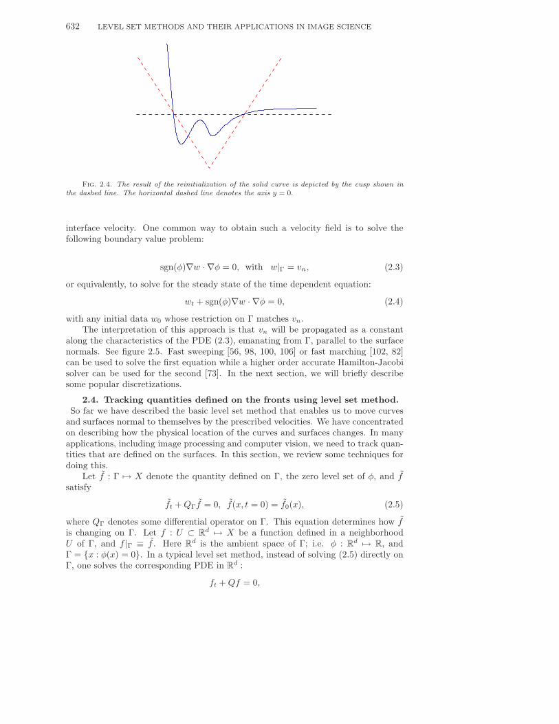
is positive, φτ < 0 whenever |∇φ| > 1; therefore, the value of φ will decrease, andconsequently, |∇φ| will become closer to 1. Notice that φτ ≡ 0 wherever φ0 ≡ 0, sincesgn(0) = 0. See figure 2.4.

Another equivalent approach is to solve the eikonal equation

|∇φ| = 1

with the boundary condition φ = 0 on φ0 = 0. A common numerical approach, e.g.[76] is to run distance reinitialization (2.4) with a high order accurate method for ashort amount of time, so that in a thin tube around φ0 = 0, φ is now the distancefunction. Then fix the values of φ in this tube as boundary conditions, and use fastsweeping or fast marching methods to solve the eikonal equations. We shall discussthe sweeping method in the next section.

We remark first that for most applications, the reinitialization is only neededfor a neighborhood around the zero level set, and the diameter of this neighborhooddepends on the discretization of the partial derivatives in the PDE. This impliesthat only a few time steps in τ are needed. Next we note that it is important tosolve (2.2) using a high order discretization method. Otherwise, the location of theoriginal interface will be perturbed noticeably by the numerical diffusion. Finally,reinitialization globally in the computational domain will prevent new zero contoursfrom appearing. Thus, one needs to be careful if emergence of new level contours is ofinterest. In many image segmentation tasks, this is important, and we shall commenton this in a later section.

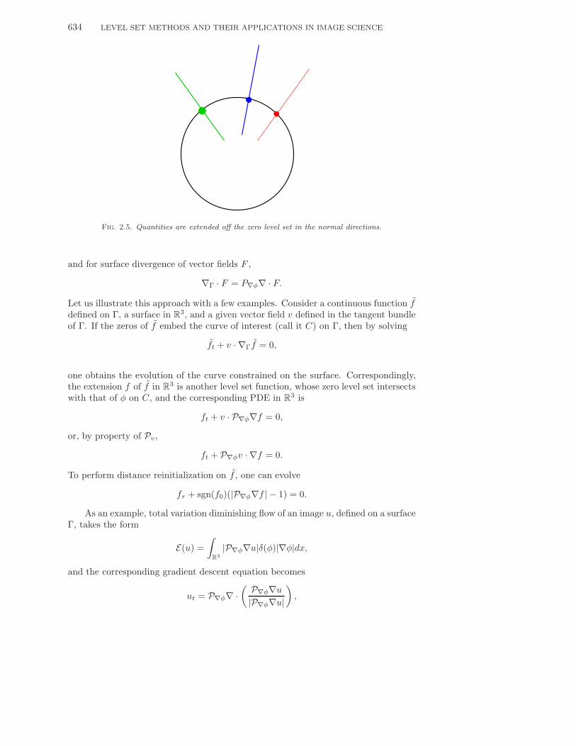
2.3. Extending quantities off the normals of the interface. In manymodels, one can only derive the interface velocity vn in equation (2.1) along Γ. It isnecessary to create a continuous velocity field defined on the whole domain Ω or atleast in a tubular neighborhood of Γ whose restriction on Γ agrees with the known


Fig. 2.4. The result of the reinitialization of the solid curve is depicted by the cusp shown inthe dashed line. The horizontal dashed line denotes the axis y = 0.

interface velocity. One common way to obtain such a velocity field is to solve thefollowing boundary value problem:

sgn(φ)∇w · ∇φ = 0, with w|Γ = vn, (2.3)

or equivalently, to solve for the steady state of the time dependent equation:

wt + sgn(φ)∇w · ∇φ = 0, (2.4)

with any initial data w0 whose restriction on Γ matches vn.The interpretation of this approach is that vn will be propagated as a constant

along the characteristics of the PDE (2.3), emanating from Γ, parallel to the surfacenormals. See figure 2.5. Fast sweeping [56, 98, 100, 106] or fast marching [102, 82]can be used to solve the first equation while a higher order accurate Hamilton-Jacobisolver can be used for the second [73]. In the next section, we will briefly describesome popular discretizations.

2.4. Tracking quantities defined on the fronts using level set method.So far we have described the basic level set method that enables us to move curves

and surfaces normal to themselves by the prescribed velocities. We have concentratedon describing how the physical location of the curves and surfaces changes. In manyapplications, including image processing and computer vision, we need to track quan-tities that are defined on the surfaces. In this section, we review some techniques fordoing this.

Let f : Γ → X denote the quantity defined on Γ, the zero level set of φ, and fsatisfy

ft +QΓf = 0, f(x, t = 0) = f0(x), (2.5)

where QΓ denotes some differential operator on Γ. This equation determines how fis changing on Γ. Let f : U ⊂ R

d → X be a function defined in a neighborhoodU of Γ, and f |Γ ≡ f . Here R

d is the ambient space of Γ; i.e. φ : Rd → R, and

Γ = x : φ(x) = 0. In a typical level set method, instead of solving (2.5) directly onΓ, one solves the corresponding PDE in R

d :

ft +Qf = 0,


so that the restriction of f(t) to Γ matches with f(t) for t ≥ 0. At this point, it isnatural to ask what Q is, given the QΓ? In many applications, the form of Q is thecenter of the study, and it might be more convenient to track an alternative quantity,g in order to obtain an equation that is easier to solve. See the recent paper [54] forsuch an example. In the next paragraph, we discuss another example of this situation.

Of the surfaces. In [48], Osher and Harabetian introduced a method for trackingthe parametrization of closed curves. Let φ denote the level set function that embedsthe surface of interest. The idea is to introduce an auxiliary function ψ such that(φ, ψ) forms a coordinate system near the zero level set of φ.

Let the family of closed curves Γ(s, t) = (x(s, t), y(s, t)) be parameterized by sand t. We want to evolve for example, Γ(s, 0) to time t, by the level set functions:

φ(x(s, t), y(s, t), t) ≡ 0, ψ(x(s, t), y(s, t), t) ≡ s.

However, ψ is not a single valued function over a closed curve if it is defined this way.The authors then proposed to evolve the Jacobian

J = det[ϕx ϕy

ψx ψy

]

instead of ψ to circumvent this problem. J has to be nonzero so that we can express(xs, ys) by (−φy, φx)/J. Thus, in order to track the tangential motion we evolve

Jt + ∇ · (Jv) = 0

in addition to

φt + v · ∇φ = 0.

Finally, we briefly describe the systematic approach that was pioneered in Cheng’sthesis [21], and later on in [7] for solving PDE’s on surfaces for image processingpurpose. A similar approach was adopted by [109] to study surfactants on interfacesthat move in time. For simplicity, we assume the zero level set to be fixed in time.

Consider the surface gradient QΓ = ∇Γ that maps scalar functions defined on Γto the tangent bundle of Γ. The key notion is to replace ∇Γ by a suitable projectionof the gradient operator ∇ in R

d. The corresponding projection operator is a linearoperator defined by:

Pv = I − v ⊗ v

|v|2 ,

or equivalently, as a matrix, Pv can be written as

(Pv)ij = δij − vivj

|v|2 ,

where v is a vector in Rd, and δij is the Kronecker delta function. For x ∈ Γ, and v

the normal of Γ at x, Pv projects vectors onto the tangent plane of Γ at x.Recall that Γ = φ = 0, and ∇φ is parallel to the normal of Γ. It can be proved

that ∇Γ and P∇φ∇ are equivalent on Γ. Thus, for scalar functions f ,

∇Γf = P∇φ∇f,


Fig. 2.5. Quantities are extended off the zero level set in the normal directions.

and for surface divergence of vector fields F ,

∇Γ · F = P∇φ∇ · F.Let us illustrate this approach with a few examples. Consider a continuous function fdefined on Γ, a surface in R

3, and a given vector field v defined in the tangent bundleof Γ. If the zeros of f embed the curve of interest (call it C) on Γ, then by solving

ft + v · ∇Γf = 0,

one obtains the evolution of the curve constrained on the surface. Correspondingly,the extension f of f in R

3 is another level set function, whose zero level set intersectswith that of φ on C, and the corresponding PDE in R

3 is

ft + v · P∇φ∇f = 0,

or, by property of Pv,

ft + P∇φv · ∇f = 0.

To perform distance reinitialization on f , one can evolve

fτ + sgn(f0)(|P∇φ∇f | − 1) = 0.

As an example, total variation diminishing flow of an image u, defined on a surfaceΓ, takes the form

E(u) =∫

R3|P∇φ∇u|δ(φ)|∇φ|dx,

and the corresponding gradient descent equation becomes

ut = P∇φ∇ ·( P∇φ∇u|P∇φ∇u|

),


where the right hand side corresponds to the geodesic curvature, and can also bewritten as

∇ ·( P∇φ∇u|P∇φ∇u| |∇φ|

)1

|∇φ| .

2.5. Limitations of the Level Set Methods. The original idea in thelevel set method is to use the sign of a given function to separate the given domaininto two disjoint regions, and use the continuity of the level set function near its zeroto define the boundary of these disjoint regions. One realizes that it can be morecomplicated to extend this idea to handle non-simple curves, and multiple phases.An equally important issue is to solve the problem at hand in obtaining a reasonablequality without excessive complexity. We refer the readers to [87, 103, 107] for levelset methods for multiple phases, [11, 66] for higher codimensions and [86] for opencurves, and [76, 93, 92] for localization. We also refer to [34] for a hybrid particle levelset method that is designed to lessen the numerical diffusion effect for some class ofproblems.

3. Numerics for conservation laws and Hamilton-Jacobi EquationsNumerical solution of conservation laws has been an active field of research for

quite some time. In particular, UCLA researchers have been major contributors tothe field. The finite difference methods commonly used in the level set methods(in particular, those related to Hamilton-Jacobi equations) are developed under thegeneral philosophy of the Godunov procedure and the nonlinear ENO reconstructiontechniques for avoiding oscillations in calculations. As a result, upwinding and ENOinterpolations become the indispensable parts of the algorithms documented here.

In what follows, we will first describe the Godunov procedure in the context ofsolving conservation laws and Hamilton-Jacobi equations. We will also describe theENO interpolation and compare the differences between its usage in conservation lawsschemes and in Hamilton-Jacobi solvers. We refer the details to the book of Osherand Fedkiw [68] and the extensive references therein.

Let us introduce some notations that we shall use in this section. Let φni,j denote

the value of xi,j = (x0 + i∆x, y0 + j∆y) ∈ Ω at time tn = t0 +n ·∆t. We shall assumethat ∆x = ∆y.

Definition 3.1. (Finite difference operators) Given the values of u on the grid wefirst define the forward and backward difference operators:

D±x ui,j := ±ui±1,j − ui,j

∆x,

and

D±y ui,j := ±ui,j±1 − ui,j

∆y;

also the central difference operators:

D0xui,j :=

ui+1,j − ui−1,j

2∆x,

and

D0yui,j :=

ui,j+1 − ui,j−1

2∆y.


3.1. The Godunov procedure. The Godunov procedure [46] developed forconservation laws started by looking at grid values as cell averages of the solution attime tn. We then “build” a piecewise constant function whose value in each cell isthe cell average. We solve the Riemann problem at cell boundaries “exactly” for anappropriate time step ∆t. This involves following the characteristics and making surethat the Rankine-Hugoniot and entropy conditions are satisfied. Finally, we averagethe function at t = tn + ∆t in each cell, and repeat the above steps.

In the context of certain conventional Hamilton-Jacobi equations, piecewise con-stant cell averages are replaced by a piecewise linear function that is continuous atthe cell boundaries, and point values are updated. This is described in [4].

In high order schemes, cell averages are replaced by more accurate nonoscillatoryreconstruction on the functions or the fluxes. We perform this reconstruction byENO/WENO methods.

3.2. ENO/WENO interpolation. We want to approximate the value ofthe function f in the interval Ii := [xi− 1

2, xi+ 1

2], using the given values (or averaged

values) of f on the grid nodes xi and its neighbors. Two commonly used methodsto get a k-th order approximation of f in Ii are spectral interpolation that is basedon Fourier expansions and fixed order polynomial interpolation. Both approachesproduce oscillations near the jumps in the function values. We will not comment onthe Fourier based methods since the they are not particularly useful in this connection.Conventional polynomial interpolations usually use the function values on all the gridpoints within a certain fixed distance from xi, regardless of the smoothness of theinterpolated function. ENO interpolation, on the other hand, is a nonlinear procedurethat is built on a “progression” of Newton’s divided differences. By “progression”,we mean that the procedure starts by building a linear reconstruction of f in Ii usingeither f(xi) and f(xi−1) or f(xi) and f(xi+1), depending on which pair of values willgive a smoother reconstruction. Suppose the reconstruction from f(xi) and f(xi−1)is selected, we then carry out the reconstruction using the values of f on eitherxi−2, xi−1, xi or xi−1, xi, xi+1. This procedure is iterated until the desired order ofapproximation is achieved. Newton’s interpolation is natural in this framework, sinceone can incrementally compute the divided differences for interpolation. In addition,we can use the values of the divided differences as an indicator of the smoothness ofthe functions in the intervals formed by the grid points that are considered as stencil.

For conservative schemes approximating conservation laws, this ENO reconstruc-tion is performed on the flux function f or the cell averages u by first reconstructingthe integral of the solution u. For Hamilton-Jacobi equations, we perform the ENOreconstruction on the solution u.

In the ENO reconstruction procedure, only one of the k candidate stencils (gridpoints used for the construction of the scheme) covering 2k− 1 cells is actually used.If the function is smooth in the neighborhood of this 2k − 1 cells, we can actuallyget a (2k − 1)-th order approximation, if we use all these grid values. This is theidea behind the WENO reconstruction. In short, WENO reconstruction uses a con-vex linear combination of all the potential stencils. The weights in the combinationare determined so that the WENO reconstruction procedure behaves like ENO neardiscontinuities. As a result, WENO method use smaller stencils to achieve the sameorder of accuracy as ENO in smooth regions. Currently, our choice of scheme is the5th order WENO. For details, we refer to the original papers [32, 49, 52, 59, 84, 85],and the review articles [83]. Recently, Shu and Balsara [3] developed even higherorder WENO reconstructions.


There are successful adaptations of this ENO idea/philosophy to other frame-works. See [16, 19] for ENO wavelet decompositions for image processing, and [24]for an application of the ENO philosophy in Discontinuous Galerkin methods.

3.3. Numerics for equations with Hamiltonians H(x, u, p) nondecreasingin u. We repeat here that any discussion of the numerical schemes cannot bedetached from the solution theory of the equation in questions. This is especiallyimportant for nonlinear equations, since in general, discontinuities in the functionvalues or in the derivatives develop in finite time. We are usually seeking a particulartype of weak solution.

In 1983, Crandall and Lions introduced viscosity solution theory for a class ofHamilton-Jacobi Equations requiring Lipschitz continuous initial data and for whichthe Hamiltonians H(x, u, p) is Lipschitz continuous and non-decreasing in u. Laterin [25] in 1984, they proved the convergence to the viscosity solution of monotone,consistent schemes for Hamilton-Jacobi Equations with H independent of x and u.Souganidis [89] extended the results to include variable coefficients. Osher and Sethiancontributed to the numerics of Hamilton-Jacobi Equation in their level set paper in1988 [72]. This line of work was later generalized and completed in the paper byOsher and Shu [73] in 1993, in which the authors provided a family of numericalHamiltonians analogous to the ENO schemes for conservation laws. WENO schemesusing the numerical Hamiltonians described in [73] were introduced in [52]. Themethod of lines using TVD Runge-Kutta time discretization is used [84]. We firstdiscretize the spatial derivatives and compute the appropriate approximation to theHamiltonians,

H(p−, p+; q−, q+),

with p±, q± representing the left/right approximations of the derivatives, obtainedfrom ENO/WENO reconstruction of the solution. They are higher order versions ofthe forward and backward divided differences of the grid functions:

p± ∼ D±x ui,j := ±ui±1,j − ui,j

∆x,

and

q± ∼ D±y ui,j := ±ui,j±1 − ui,j

∆y.

3.4. The Lax-Friedrichs schemes for the level set equation. Followingthe methods originally conceived for HJ equations φt + H(Dφ) = 0 in [73], see also[72], and suppressing the dependence of H on x and y, we use the Local Lax-Friedrichs(LLF) flux

HLLF (p+, p−, q+, q−) = H(p+ + p−

2,q+ + q−

2)

−12αx(p+, p−)(p+ − p−) − 1

2αy(q+, q−)(q+ − q−),

for the approximation of H. In the above scheme,

αx(p+, p−) = maxp∈I((p+,p−),C≤q≤D

|Hφx(p, q)|,


αy(q+, q−) = maxq∈I((q+,q−),A≤p≤B

|Hφy(p, q)|,

I(a, b) = [min(a, b),max(a, b)],

and p±, q± are the forward and backward approximations of φx and φy respectively.

3.5. Curvatures. In many applications, the curvature term

∇ · ∇φ|∇φ| or ∇ · ∇u

|∇u|for the level set function φ or the image function u appears as a regularization. Thisterm is approximated by finite differencing centered at each grid point. For con-venience, let (nx

i,j , nyi,j) denote the values of ∇u/|∇u|ε at the grid point xi,j , and

∇u/|∇u|ε is a smooth approximation of ∇u/|∇u| (This avoids the issue of singularityat |∇u| and is better for numerical computations). The curvature κi,j is approximatedby

κεi,j :=

nxi+1/2,j − nx

i−1/2,j

∆x+ny

i,j+1/2 − nyi,j−1/2

∆y,

and

nxi±1/2,j : =

D±x ui,j√

(D±x ui,j)2 +D0

y(S±x ui,j)2 + ε2

,

nεi,j±1/2 :=

D±y ui,j√

D0x(S±

y ui,j)2 + (D±y ui,j)2 + ε2

,

where

S±x ui,j =

ui±1,j + ui,j

2, and S±

y ui,j =ui,j±1 + ui,j

2

are the averaging operators in the x and y direction and ε > 0 is quite small.

3.6. Time discretization. From the previous subsections, we know how todiscretize the terms involving spatial derivatives. What remains is to discretize intime in order to evolve the system; i.e. we need to solve the following ODE system:

∂

∂tφi,j = −H(φn

i−1,j , φni+1,j , φ

ni,j , φ

ni,j−1, φ

ni,j+1),

where H is the numerical approximation of H(x, φ,Dφ,D2φ). For example, if we uselocal Lax-Friedrichs for H(φx, φy), and forward Euler for time, we end up having:

φn+1i,j = φn

i,j − ∆tHLLF (xi, yj , Dx+φ

ni,j , D

x−φ

ni,j). (3.1)

Typically, we use 3rd order TVD Runge-Kutta scheme of [84], or the fourth orderschemes of [90] to evolve the system, since higher order accuracy can be achievedwhile using larger time steps. To keep this description self-contained, we describe the3rd order TVD RK scheme below: we wish to advance ut = rhs(u) from tnto tn+1.

1. u1 = un + ∆t · rhs(un);2. u2 = 3

4un + 1

4u1 + 14∆t · rhs(u1);

3. un+1 = 13u

n + 23u2 + 2

3∆t · rhs(u2).


3.7. Algorithms for constructing the distance function. In the followingsubsections, we review some of the solution methods for the eikonal equation:

|∇u| = r(x, y), u|Γ = 0.

We present a fast Gauss-Seidel type iteration method which utilizes a monotone up-wind Godunov flux for the Hamiltonian. We show numerically that this algorithmcan be applied directly to equations of the above type with variable coefficients.

3.8. Solving eikonal equations. In geometrical optics [57], the eikonalequation

√φ2

x + φ2y = r(x, y) (3.2)

is derived from the leading term in an asymptotic expansion

eiω(φ(x,y)−t)∞∑

j=0

Aj(x, y, t)(iω)−j

of the wave equation:

wtt − c2(x, y)(wxx + wyy) = 0,

where r(x, y) = 1/|c(x, y)|, is the function of slowness. The level sets of the solutionφ can be thus be interpreted as the first arrival time of the wave front that is initiallyΓ. It can also be interpreted as the “distance” function to Γ.

We first restrict our attention to the case in which r = 1. Let Γ be a closed subsetof R

2. It can be shown easily that the distance function defined by

d(x) = dist (x,Γ) := minp∈Γ

|x − p|, x = (x, y) ∈ R2,

is the viscosity solution to equation (3.2) with the boundary condition

φ(x, y) = 0 for (x, y) ∈ Γ.

Rouy and Tourin [78] proved the convergence to the viscosity solution of an it-erative method solving equation (3.2) with the Godunov numerical Hamiltonian ap-proximating |∇φ|. The Godunov numerical Hamiltonian function can be written inthe following simple form for this eikonal equation:

HG(p−, p+, q−, q+) =√

maxp+−, p

−+2 + maxq+−, q−+2, (3.3)

where p± = Dx±φi,j , q± = Dy

±φi,j , and x+ = max(x, 0), x− = −min(x, 0). The taskis then to solve

HG = 1

on the grid.Osher [65] provided a link to time dependent eikonal equations by proving that

the t-level set of φ(x, y) is the zero level set of the viscosity solution of the evolutionequation at time t

ψt + |∇ψ| = 0


with appropriate initial conditions. In fact, the same is true for a very general class ofHamilton-Jacobi equations (see [65]). As a consequence, one can try to solve the time-dependent equation by the level set formulation [72] with high order approximationson the partial derivatives[73, 52]. Crandall and Lions proved that the discrete solutionobtained with a consistent, monotone Hamiltonian converges to the desired viscositysolution [25].

Tsitsiklis [102] combined heap sort with a variant of the classical Dijkstra algo-rithm to solve the steady state equation of the more general problem

|∇φ| = r(x).

This was later rederived in [82] and [50]. It has become known as the fast marchingmethod whose complexity is O(N log(N)), where N is the number of grid points.Osher and Helmsen[70] have extended the fast marching type method to somewhatmore general Hamilton-Jacobi equations. Since the fast marching method is by nowwell known, we will not give details here on its implementation in this paper.

3.9. The sweeping idea. Danielsson [27] proposed an algorithm to computeEuclidean distance to a subset of grid points on a two dimensional grid by visitingeach grid node in some predefined order. In [9], Boue and Dupuis suggest a similar“sweeping” approach to solve the steady state equation which, by experience, resultsin a O(N) algorithm for the problem at hand. This “sweeping” approach has recentlybeen used in [98] and [108] to compute the distance function to an arbitrary data setin computer vision. In [106], it was proven that the fast sweeping algorithm achievesa reasonable accuracy in a (small) finite number of iterations independent of gridsize. Using this “sweeping” approach, the complexity of the algorithms drops fromO(N logN) in the fast marching to O(N), and the implementation of the algorithmsbecomes a bit easier than the fast marching method in that no heap sort is needed.

This sweeping idea is best illustrated by solving the eikonal equation in [0, 1] :

|ux| = 1, u(0) = u(1) = 0.

Let ui = u(xi) be the grid values and x0 = 0, xn = 1. We then solve the discretizednonlinear system

√max(max(D−ui, 0)2,min(D+ui, 0)2) = 1, u0 = un = 0 (3.4)

by our sweeping approach. Let us begin by sweeping from −1 to 1, i.e. we update ui

from i = 0 increasing to i = n. This is “equivalent” to following the characteristicsemanating from x0. Let u(1)

i denote the grid values after this sweep. We then have

u(1)i =

i/n, if i < n1/n i = n

.

In the second sweep, we update ui from i = n decreasing to 0, using u(1)i . During this

sweep, we follow the characteristics emanating from xn. The use of (3.4) is essential,since it determines what happens when two characteristics cross each other. It is thennot hard to see that after the second sweep,

ui =

i/n, if i ≤ n/2(n− i)/n otherwise.


Thus, to update uo, one only uses the immediate neighboring grid values and doesnot need the heap sort data structure. More importantly, the algorithm follows thecharacteristics with certain directions simultaneously, in a parallel way, instead of asequential way as in the fast marching method. The Godunov flux is essential in thealgorithm, since it determines what neighboring grid values should be used to updateu on a given grid node o. At least in the examples presented, we only need to solvea simple quadratic equation and run some simple tests to determine the value to beupdated. This simple procedure is performed in each sweep, and solution is obtainedafter a few sweeps.

3.10. Generalized closest point algorithms. In this subsection, we de-scribe an algorithm that can be applied for constructing a level set implicit repre-sentation for a surface which is defined explicitly. It can also be used to extend theinterface velocity to the whole computational domain.

In the spirit of the Steinhoff et.al. Dynamic Surface Extension [91], we can definefunctions that map each point in R

3 to the space of (local) representations of surfaces(heretherto referred as surface elements). We can further define the distance of apoint P and a surface element S

dist(P,S) := miny∈S

(P, y).

The ‘surface element’ can be for example the tangent plane, the curvature, or a NURBdescription of the surface.

Instead of propagating distance values away from the interface, we propagatethe surface element information along the characteristics and impose conditions thatenforce the first arrival property of the viscosity solution of the eikonal equation. Thechallenge is to compute the exact distance from a given surface element and to derivethe “upwinding” criteria for propagating the surface information throughout the grids.

Given a smooth parameterized surface Σ : Is × It → R3, our algorithm provides

good initial guess for Newton’s iterations on the orthogonality identity:

F (s∗, t∗;x) =(

(x − Σ(s∗, t∗)) · Σs(s∗, t∗)(x − Σ(s∗, t∗)) · Σt(s∗, t∗)

)= 0,

where Σ(s∗, t∗) is the closest point on the surface to x. The initial guess in this caseis simply the closest point of the neighbors of x.

Let W denote the function that maps each point in space to its closest surfaceelement on S. We can then write the algorithm as follows:

Algorithm: Let u be the distance function on the grids, and W be the corre-sponding generalized closest point function.

1. Initialize: give the exact distance to u, and the exact surface elements to Wat grids near Γ. Mark them so they will not be updated. Mark all other gridvalues as ∞.

2. Iterate through each grid point E with index (i,j,k) in each sweeping directionor according to the fast marching heap sort.

3. For each neighbor Pl of E, compute utmpl = dist(E,W (Pl))

4. If dist(E,W (Pl)) < mink u(Pk), set utmpl = ∞. This is to enforce the mono-

tonicity of the solution.5. Set u(E) = minl u

tmpl = utmp

λ and W (E) = W (Pλ).This procedure can be used e.g., to convert triangulated surfaces to implicit surfaces.


3.11. Further generalizations. For further generalizations of the sweepingmethod to solve more complicated Hamilton-Jacobi equations, such as those whicharise in computing distance on a manifold:

H(ux, uy) =√au2

x + bu2y + 2cuxuy = r(x, y), for a, b > 0, ab > c2,

and the equations using Bellman’s formulae, we refer the readers to the recent papers[100, 56]. Recently, a very simple sweeping algorithm, based on the Lax-Friedrichsscheme, has been shown to work in great generality [55].

4. Segmentation AlgorithmsThe task of image segmentation is to find a collection of non-overlapping subre-

gions of a given image. In medical imaging, for example, one might want to segmentthe tumor or the white matter of a brain from a given MRI image. In airport screen-ing, one might wish to segment certain “sensitive” shapes, such as guns. There aremany other obvious applications. Mathematically, given an image u : Ω ⊂ R

2(orR

3)→R+, we want to find closed sets Ωi satisfying

Ω =N−1⋃i=0

Ωi, andN−1⋂i=0

Ω(0)i = ∅,

such that F(u,Ωi) = 0, where F is some functional that defines the segmentationgoals. Here, Ω(0)

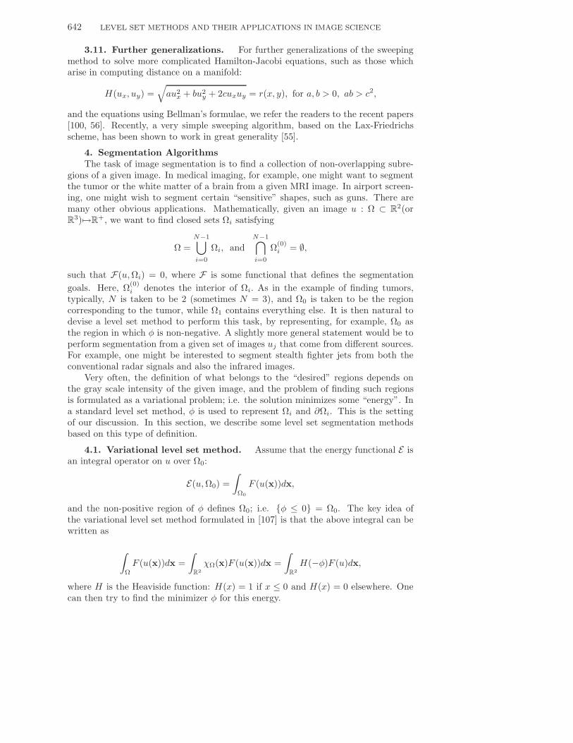
i denotes the interior of Ωi. As in the example of finding tumors,typically, N is taken to be 2 (sometimes N = 3), and Ω0 is taken to be the regioncorresponding to the tumor, while Ω1 contains everything else. It is then natural todevise a level set method to perform this task, by representing, for example, Ω0 asthe region in which φ is non-negative. A slightly more general statement would be toperform segmentation from a given set of images uj that come from different sources.For example, one might be interested to segment stealth fighter jets from both theconventional radar signals and also the infrared images.

Very often, the definition of what belongs to the “desired” regions depends onthe gray scale intensity of the given image, and the problem of finding such regionsis formulated as a variational problem; i.e. the solution minimizes some “energy”. Ina standard level set method, φ is used to represent Ωi and ∂Ωi. This is the settingof our discussion. In this section, we describe some level set segmentation methodsbased on this type of definition.

4.1. Variational level set method. Assume that the energy functional E isan integral operator on u over Ω0:

E(u,Ω0) =∫

Ω0

F (u(x))dx,

and the non-positive region of φ defines Ω0; i.e. φ ≤ 0 = Ω0. The key idea ofthe variational level set method formulated in [107] is that the above integral can bewritten as

∫Ω

F (u(x))dx =∫

R2χΩ(x)F (u(x))dx =

∫R2H(−φ)F (u)dx,

where H is the Heaviside function: H(x) = 1 if x ≤ 0 and H(x) = 0 elsewhere. Onecan then try to find the minimizer φ for this energy.


4.2. The Chan-Vese algorithm. This is closely related to the classicalMumford-Shah algorithm [63], but uses a simple level set framework for its implemen-tation. We present the original Chan-Vese segmentation algorithm [18], and discussvarious aspects of this algorithm.

4.2.1. Basic formulation. The minimization problem is:

minφ∈BV (Ω),c1,c2∈R+

E(φ, c1, c2;u0),

where the energy is defined as

E(φ, c1, c2;u0) = µ

∫Ω

δ(φ)|∇φ|dx +

λ1

∫Ω

|u0 − c1|2H(φ)dx + λ2

∫Ω

|u0 − c2|2(1 −H(φ))dx. (4.1)

Intuitively, one can interpret from this energy that each segment is defined as thesubregions of the images over which the average of the given image is “closest” to theimage value itself in L2-norm. The first term in the energy measures the arclengthof the segment boundaries. Thus, minimizing this quantity provides stability of thealgorithm as well as preventing fractal like boundaries from appearing.

If one regularizes the δ function and the Heaviside function by two suitable smoothfunctions δε and Hε, then formally, the Euler-Lagrange equations can be written as

∂φE = −δε(φ)[µ∇ · ∇φ

|∇φ| − ν − λ1(u0 − c1)2 + λ2(u0 − c2)2]

= 0, (4.2)

with natural boundary condition

δε(φ)|∇φ|

∂φ

∂n= 0 on ∂Ω.

c1(φ) =

∫Ωu0(x)Hε(φ(x))dx∫ΩHε(φ(x))dx

, (4.3)

and

c2(φ) =

∫Ω u0(x)(1 −Hε(φ(x)))dx∫

Ω(1 −Hε(φ(x)))dx

. (4.4)

4.2.2. Discretization. A common approach to solve the minimization prob-lem is to perform gradient descent on the regularized Euler-Lagrange equation (4.2);i.e. solving the following time dependent equation to steady state:

∂φ

∂t= −∂φE

= δε(φ)[µ∇ · ∇φ

|∇φ| − ν − λ1(u0 − c1)2 + λ2(u0 − c2)2]. (4.5)

Here, we remind the readers that c1(φ) and c2(φ) are defined in (4.3) and (4.4).


In Chan-Vese algorithm, the authors regularized the Heaviside function used in(4.3) and (4.4):

H2,ε(z) =12

(1 +

2π

arctan(z

ε)),

and define the delta function as the derivative of it:

δ2,ε(z) = H ′2,ε(z).

Equation (4.5) is then discretized by a semi-implicit scheme; i.e. to advance from φni,j

to φn+1i,j , the curvature term right hand side of (4.5) is discretized as described in the

previous section using the value of φni±,j± , except for the diagonal term φi,j , which uses

the implicitly defined φn+1i,j . The integrals defining c1(φ) and c2(φ) are approximated

by simple Riemann sum with the regularized Heaviside function defined above. φt

is discretized by the forward Euler method: (φn+1i,j − φn

i,j)/∆t. Therefore, the finalupdate formula can be conceptually written as

φn+1i,j =

11 + ακ

(φn

i,j +G(φni−1,j , φ

ni+1,j , φ

ni,j−1, φ

ni,j+1)

),

where ακ ≥ 0 comes from the discretization of the curvature term. If the scheme isfully explicit, ακ = 0 and G would depend on φn

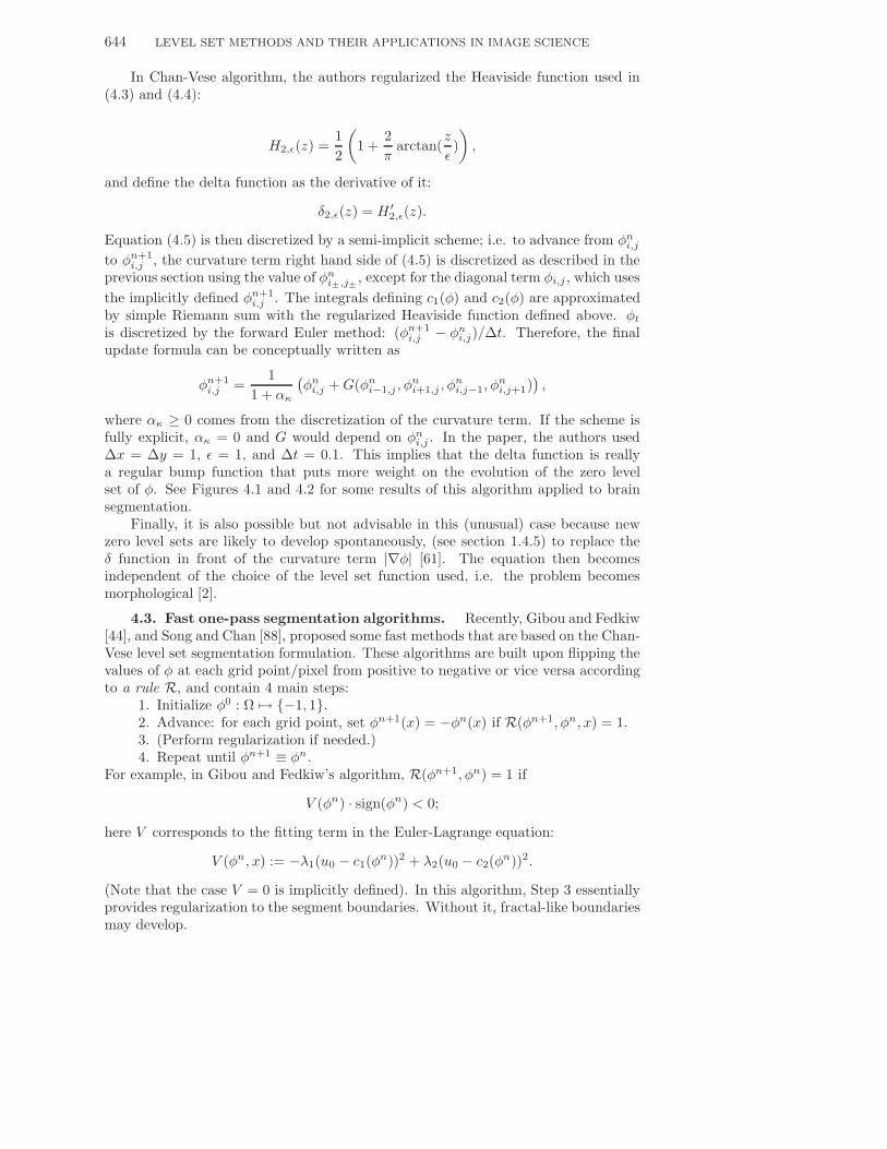
i,j . In the paper, the authors used∆x = ∆y = 1, ε = 1, and ∆t = 0.1. This implies that the delta function is reallya regular bump function that puts more weight on the evolution of the zero levelset of φ. See Figures 4.1 and 4.2 for some results of this algorithm applied to brainsegmentation.

Finally, it is also possible but not advisable in this (unusual) case because newzero level sets are likely to develop spontaneously, (see section 1.4.5) to replace theδ function in front of the curvature term |∇φ| [61]. The equation then becomesindependent of the choice of the level set function used, i.e. the problem becomesmorphological [2].

4.3. Fast one-pass segmentation algorithms. Recently, Gibou and Fedkiw[44], and Song and Chan [88], proposed some fast methods that are based on the Chan-Vese level set segmentation formulation. These algorithms are built upon flipping thevalues of φ at each grid point/pixel from positive to negative or vice versa accordingto a rule R, and contain 4 main steps:

1. Initialize φ0 : Ω → −1, 1.2. Advance: for each grid point, set φn+1(x) = −φn(x) if R(φn+1, φn, x) = 1.3. (Perform regularization if needed.)4. Repeat until φn+1 ≡ φn.

For example, in Gibou and Fedkiw’s algorithm, R(φn+1, φn) = 1 if

V (φn) · sign(φn) < 0;

here V corresponds to the fitting term in the Euler-Lagrange equation:

V (φn, x) := −λ1(u0 − c1(φn))2 + λ2(u0 − c2(φn))2.

(Note that the case V = 0 is implicitly defined). In this algorithm, Step 3 essentiallyprovides regularization to the segment boundaries. Without it, fractal-like boundariesmay develop.


Fig. 4.1. Brain segmentation in 2D.

Fig. 4.2. Brain segmentation in 3D.

In Song and Chan’s algorithm, the key observation is that only the signs of thethe level set function matter in the energy functional. This can easily be seen fromthe model defined in equation (4.1), in which one sees that the energy is a function ofH(−φ). In this algorithm, R(φn+1, φn) can be interpreted as the logical evaluationof the following inequality:

E(φn+1, c1, c2;u0) ≤ E(φn, c1, c2;u0).


Hence, the sign of φn(x) is flipped only if the energy (4.1) is non-increasing. This pro-vides stability of the algorithm when compared to Gibou and Fedkiw’s in which thereis no checking on the energy descent, at the cost of some speed of implementation.

We remark that there is a close connection between these two “level set” basedmethods to the “Γ-convergence” base methods. The Chan-Vese segmentation methodcan be approximated by the following variational problem:

Eε(u, c1, c2;u0) := µ

∫ε|∇u|2+1

εW (u)dx+λ1

∫u2(u0−c1)2+λ2

∫(1−u)2(u0−c2)2dx,

where w(u) = u2(1−u)2, and ε is a small positive number. Due to the strong potentialε−1W (u), u will quickly be attracted to either 1 or 0, and consequently, the termsu2 and (1 − u)2 correspond respectively to H(φ) and 1 −H(φ) in (4.1), and ε|∇u|2corresponds to the regularization of the length of ∂Ωi. Essentially, one can interpretthe Gibou-Fedkiw or Song-Chan algorithm as performing a one step projection to thesteady state that results from the stiff potential W . This is delineated in the currentwork of Esedoglu and Tsai [37].

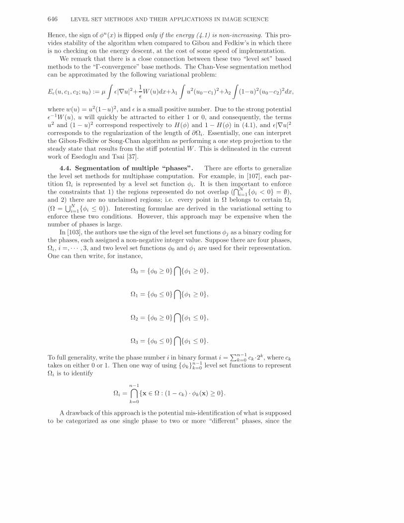
4.4. Segmentation of multiple “phases”. There are efforts to generalizethe level set methods for multiphase computation. For example, in [107], each par-tition Ωi is represented by a level set function φi. It is then important to enforcethe constraints that 1) the regions represented do not overlap (

⋂Ni=1φi < 0 = ∅),

and 2) there are no unclaimed regions; i.e. every point in Ω belongs to certain Ωi

(Ω =⋃N

i=1φi ≤ 0). Interesting formulae are derived in the variational setting toenforce these two conditions. However, this approach may be expensive when thenumber of phases is large.

In [103], the authors use the sign of the level set functions φj as a binary coding forthe phases, each assigned a non-negative integer value. Suppose there are four phases,Ωi, i =, · · · , 3, and two level set functions φ0 and φ1 are used for their representation.One can then write, for instance,

Ω0 = φ0 ≥ 0⋂

φ1 ≥ 0,

Ω1 = φ0 ≤ 0⋂

φ1 ≥ 0,

Ω2 = φ0 ≥ 0⋂

φ1 ≤ 0,

Ω3 = φ0 ≤ 0⋂

φ1 ≤ 0.

To full generality, write the phase number i in binary format i =∑n−1

k=0 ck ·2k, where cktakes on either 0 or 1. Then one way of using φkn−1

k=0 level set functions to representΩi is to identify

Ωi =n−1⋂k=0

x ∈ Ω : (1 − ck) · φk(x) ≥ 0.

A drawback of this approach is the potential mis-identification of what is supposedto be categorized as one single phase to two or more “different” phases, since the


Fig. 4.3. Initialization.

formulation really comes with 2n phases with n level set functions. In the Chan-Vese algorithm for example, it is possible that the image u has the same average intwo different segments. Another drawback is the possible miscalculation of the arclength/surface area of each phase, when two phase boundaries are forced to collapseinto one and may be given more weight than others. Related to the above drawbacks,an important but so far untouched (to the best of our knowledge) problem in thelevel set world is to determine the optimal number of phases in certain segmentationproblems.

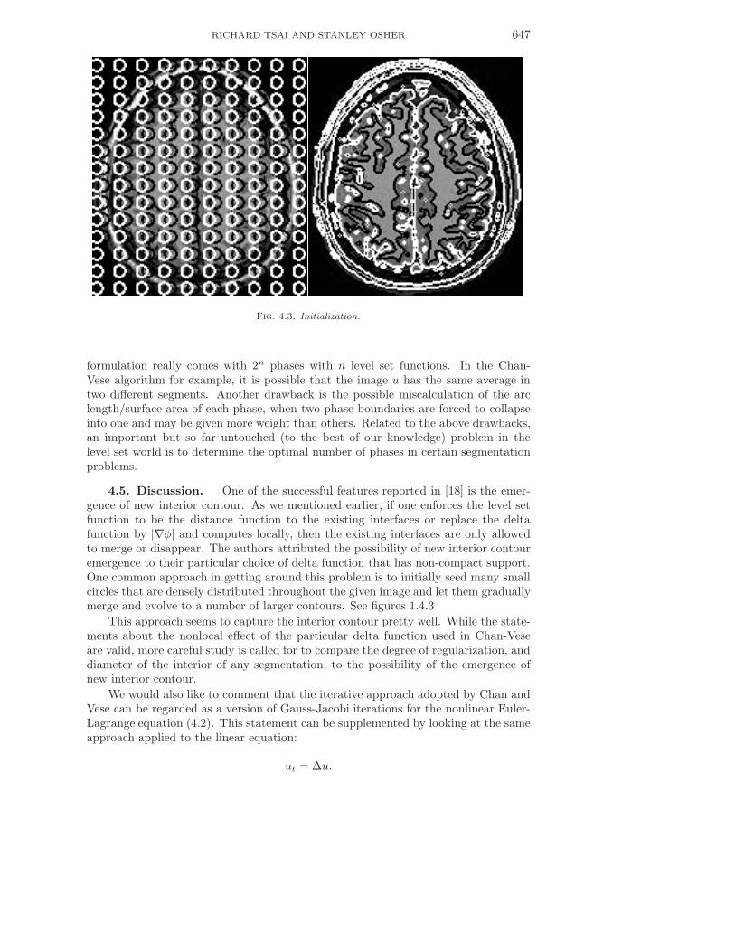
4.5. Discussion. One of the successful features reported in [18] is the emer-gence of new interior contour. As we mentioned earlier, if one enforces the level setfunction to be the distance function to the existing interfaces or replace the deltafunction by |∇φ| and computes locally, then the existing interfaces are only allowedto merge or disappear. The authors attributed the possibility of new interior contouremergence to their particular choice of delta function that has non-compact support.One common approach in getting around this problem is to initially seed many smallcircles that are densely distributed throughout the given image and let them graduallymerge and evolve to a number of larger contours. See figures 1.4.3

This approach seems to capture the interior contour pretty well. While the state-ments about the nonlocal effect of the particular delta function used in Chan-Veseare valid, more careful study is called for to compare the degree of regularization, anddiameter of the interior of any segmentation, to the possibility of the emergence ofnew interior contour.

We would also like to comment that the iterative approach adopted by Chan andVese can be regarded as a version of Gauss-Jacobi iterations for the nonlinear Euler-Lagrange equation (4.2). This statement can be supplemented by looking at the sameapproach applied to the linear equation:

ut = ∆u.


The complexity of both approaches is proportional to N2, the total number of pixels.This is verified by the computations of Song in [36]. We remark that it is possible tospeed up the gradient flow in the Chan-Vese algorithm by a splitting method describedin [43].

There are many new (and old) “level set based” segmentation algorithms thatdiscard the continuity of the level set function and propose, instead, to model thesegmentation problem as a completely discrete, pixel-by-pixel, algorithm. As in [44]and [88], these type of methods typically appear to be faster, and in some cases, moreflexible in handling multiple phases. This trend seems to be going against the origi-nal spirit and raison d’etre of PDE based level set methods for image processing —the geometry of the interface is approximated at higher order accuracy through theassumed continuity of the level set function over the grid. This fact resonates withthe criticism over phase field models for segmentation that there is no accurate repre-sentation of the interface, unless one refines the grid and resolves the stiff parameterε−1 (something that is typically impossible to do for many image applications).

One should ask the question whether accurate representation of the phase bound-aries is really needed for the problem at hand. Of course, there are applicationsin which geometrical quantities of the phase boundaries play important roles in themodel; e.g. in the disocclusion application of Nitzberg-Mumford-Shiota [64] and alsoin the applications related to Euler’s Elastica. In these type of applications, the “con-ventional” level set approach certainly has the advantage. In the cases where thegeometrical quantities are not of importance, the piecewise constant model may bequite useful.

Our last comment is on the regularization term of the level set based segmentationmethods. So far, popular choices have been the variants coming from minimizingthe length of the interface. In denoising, as we have seen, this corresponds to L1

regularization of the image gradient. It is possible that the features to be segmented,due to their origin, retain special orientations and are anisotropic. These type ofapplications exist, for example, in material sciences. In this case, one should lookinto the possible alternatives. We point out that Wulff energy is one such possiblecandidate. There, the regularization operator R is a function of the normal of theinterface, i.e. R(n) = div(γ(n)). In the common TV regularization, γ(n) = n. Werefer to details to [71, 77] and [67].

5. Pushing the LimitIn this section, we will describe recent work corresponding to the classical appli-

cations that we listed above. We will see that this new work combines different ideastogether to manipulate more complicated geometrical objects. However, the basicprinciple and spirit remains unchanged.

We start with total variation denoising. In [62], Meyer examined the total vari-ation model of [80] more closely and proposed to decompose an image, u0, into twoportions, u0 = u + v, where v contains the texture and noise parts of u0 and can bewritten as the divergence of a vector field; i.e. v = div g with the norm of v, ||v||∗defined as the infimum of L∞ norms of such vectors g. Soon afterwards, in [104] andalso [74], the authors proposed a numerical algorithm of approximating such a decom-position and combined it with other texture synthesis techniques to inpaint texturedimages [6].

In [11, 22], the authors provided a level set framework to represent and movecurves on implicit surfaces or in free three dimensional space. This framework wasthen generalized to process images and even more general quantities such as vector


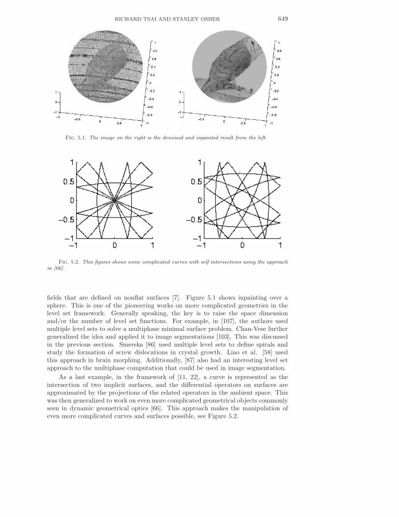
Fig. 5.1. The image on the right is the denoised and inpainted result from the left.

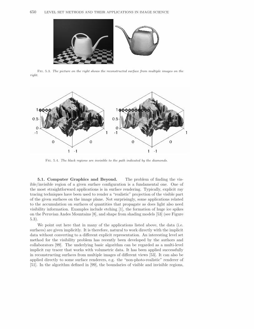
Fig. 5.2. This figures shows some complicated curves with self intersections using the approachin [66].

fields that are defined on nonflat surfaces [7]. Figure 5.1 shows inpainting over asphere. This is one of the pioneering works on more complicated geometries in thelevel set framework. Generally speaking, the key is to raise the space dimensionand/or the number of level set functions. For example, in [107], the authors usedmultiple level sets to solve a multiphase minimal surface problem. Chan-Vese furthergeneralized the idea and applied it to image segmentations [103]. This was discussedin the previous section. Smereka [86] used multiple level sets to define spirals andstudy the formation of screw dislocations in crystal growth. Liao et al. [58] usedthis approach in brain morphing. Additionally, [87] also had an interesting level setapproach to the multiphase computation that could be used in image segmentation.

As a last example, in the framework of [11, 22], a curve is represented as theintersection of two implicit surfaces, and the differential operators on surfaces areapproximated by the projections of the related operators in the ambient space. Thiswas then generalized to work on even more complicated geometrical objects commonlyseen in dynamic geometrical optics [66]. This approach makes the manipulation ofeven more complicated curves and surfaces possible, see Figure 5.2.


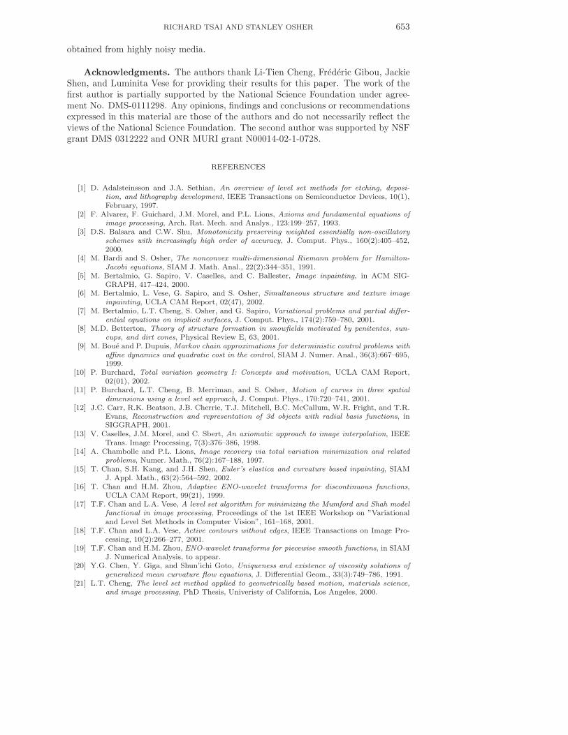
Fig. 5.3. The picture on the right shows the reconstructed surface from multiple images on theright.

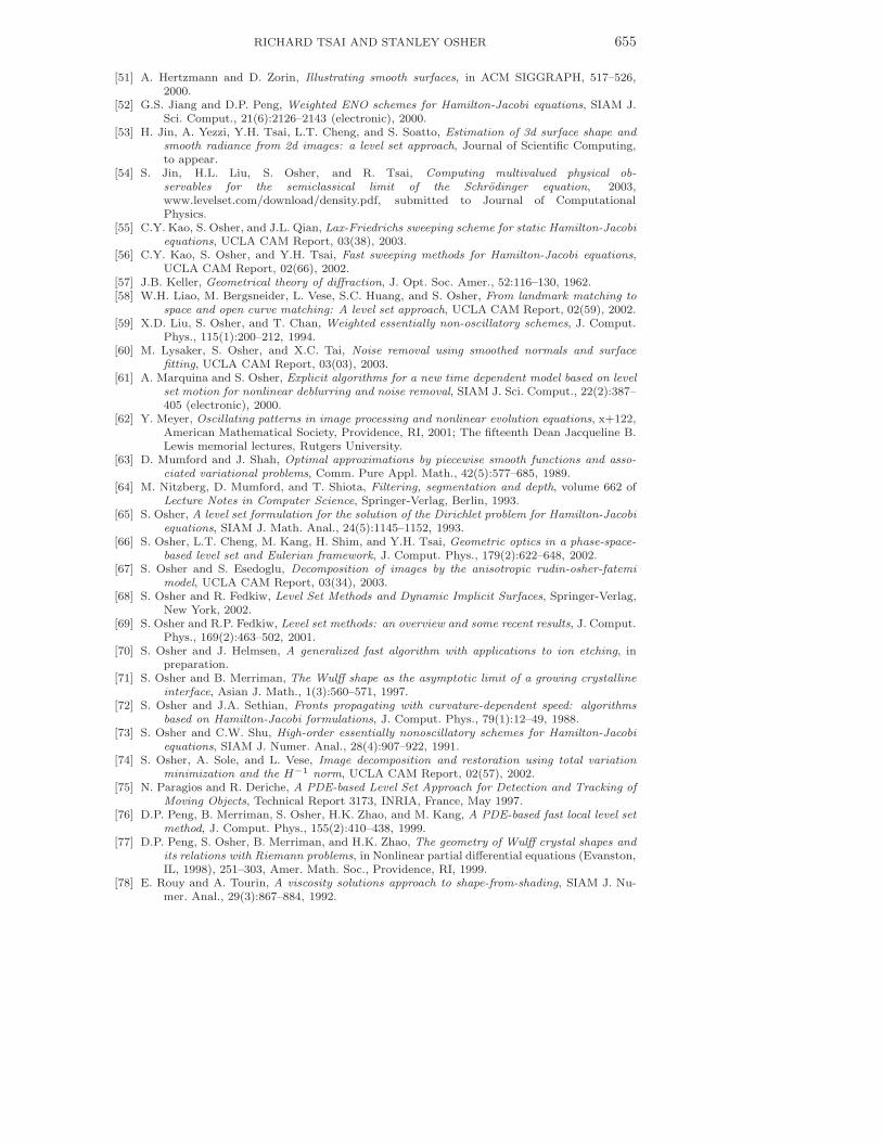
Fig. 5.4. The black regions are invisible to the path indicated by the diamonds.

5.1. Computer Graphics and Beyond. The problem of finding the vis-ible/invisible region of a given surface configuration is a fundamental one. One ofthe most straightforward applications is in surface rendering. Typically, explicit raytracing techniques have been used to render a “realistic” projection of the visible partof the given surfaces on the image plane. Not surprisingly, some applications relatedto the accumulation on surfaces of quantities that propagate as does light also needvisibility information. Examples include etching [1], the formation of huge ice spikeson the Peruvian Andes Mountains [8], and shape from shading models [53] (see Figure5.3).

We point out here that in many of the applications listed above, the data (i.e.surfaces) are given implicitly. It is therefore, natural to work directly with the implicitdata without converting to a different explicit representation. An interesting level setmethod for the visibility problem has recently been developed by the authors andcollaborators [99]. The underlying basic algorithm can be regarded as a multi-levelimplicit ray tracer that works with volumetric data. It has been applied successfullyin reconstructing surfaces from multiple images of different views [53]. It can also beapplied directly to some surface renderers, e.g. the “non-photo-realistic” renderer of[51]. In the algorithm defined in [99], the boundaries of visible and invisible regions,


−1−0.5

00.5

1

−1

−0.5

0

0.5

1

−1.5

−1

−0.5

0

0.5

1

1.5

Fig. 5.5. The blue surface borders the visible and invisible regions. The light blue and yellowcurves indicate the silhouettes and swaths.

both silhouette and swath [30], are implicitly represented in the framework of [11, 22],mentioned above. Figure 5.4 shows an accumulative visibility result of a path abovethe Grand Canyon. Figure 5.5 shows a result and the silhouette.

This implicit framework for visibility offers many other advantages. For example,the visibility information can be interpreted as the solution of simple first order PDEs


A noisy image to be inpainted. Inpainting via Mumford−Shah−Euler image model

Fig. 5.6. This is an inpainting result of [35].

and [99] offers a near optimal solution method on the grid. The dynamics of thevisibility with respect to moving vantage point or dynamic surfaces can be derivedand tracked implicitly within the same framework. Furthermore, using the sameframework and the well developed level set calculus and numerics, one can start solvingvariational problems on the visibility numerically and efficiently [97]. This will thenrelate to classical “guarding cameras” or “pursuer-evader” problems in computationalgeometry and robotics.

6. Current TrendsCurrently, higher order nonlinear PDEs are increasingly appearing in image sci-

ence. For example, in image inpainting of [15, 35, 60], a fourth order PDE is derivedfrom regularizing the level set curvature of a given image. Figure 5.6 shows an in-painting result from [35].

In computer graphics, Tasdizen et al. [95] proposed to perform anisotropic dif-fusion on the normals of a given level set surface model. In general, fourth orderequations are much harder to analyze, since they generally do not have a maximumprinciple as second order parabolic equations do. Another interesting paper of Bur-chard [10] discusses the diffusion operators constrained in color space.

There is also a trend of devising extremely fast (almost one-pass and discrete)algorithms for image science applications from level set PDE models. This began in[44, 88].

Multiscale methods have been successfully applied to several different applica-tions in image science. For example, wavelet analysis has been quite successful inimage compression. Multigrid methods provide fast algorithms to solve certain linearequations. Fast Multipole Methods also have been used in image science, see e.g.[12]. Recently, a general framework (HMM) for a class of multiscale problems hasbeen advocated by W. E and B. Engquist [31]. An HMM-level set method for frontpropagation in random media is introduced by [23]. The authors believe that a com-bined multiscale-level set method will be useful in modeling image sequences that are


obtained from highly noisy media.

Acknowledgments. The authors thank Li-Tien Cheng, Frederic Gibou, JackieShen, and Luminita Vese for providing their results for this paper. The work of thefirst author is partially supported by the National Science Foundation under agree-ment No. DMS-0111298. Any opinions, findings and conclusions or recommendationsexpressed in this material are those of the authors and do not necessarily reflect theviews of the National Science Foundation. The second author was supported by NSFgrant DMS 0312222 and ONR MURI grant N00014-02-1-0728.

REFERENCES

[1] D. Adalsteinsson and J.A. Sethian, An overview of level set methods for etching, deposi-tion, and lithography development, IEEE Transactions on Semiconductor Devices, 10(1),February, 1997.

[2] F. Alvarez, F. Guichard, J.M. Morel, and P.L. Lions, Axioms and fundamental equations ofimage processing, Arch. Rat. Mech. and Analys., 123:199–257, 1993.

[3] D.S. Balsara and C.W. Shu, Monotonicity preserving weighted essentially non-oscillatoryschemes with increasingly high order of accuracy, J. Comput. Phys., 160(2):405–452,2000.

[4] M. Bardi and S. Osher, The nonconvex multi-dimensional Riemann problem for Hamilton-Jacobi equations, SIAM J. Math. Anal., 22(2):344–351, 1991.

[5] M. Bertalmio, G. Sapiro, V. Caselles, and C. Ballester, Image inpainting, in ACM SIG-GRAPH, 417–424, 2000.

[6] M. Bertalmio, L. Vese, G. Sapiro, and S. Osher, Simultaneous structure and texture imageinpainting, UCLA CAM Report, 02(47), 2002.

[7] M. Bertalmio, L.T. Cheng, S. Osher, and G. Sapiro, Variational problems and partial differ-ential equations on implicit surfaces, J. Comput. Phys., 174(2):759–780, 2001.

[8] M.D. Betterton, Theory of structure formation in snowfields motivated by penitentes, sun-cups, and dirt cones, Physical Review E, 63, 2001.

[9] M. Boue and P. Dupuis, Markov chain approximations for deterministic control problems withaffine dynamics and quadratic cost in the control, SIAM J. Numer. Anal., 36(3):667–695,1999.

[10] P. Burchard, Total variation geometry I: Concepts and motivation, UCLA CAM Report,02(01), 2002.

[11] P. Burchard, L.T. Cheng, B. Merriman, and S. Osher, Motion of curves in three spatialdimensions using a level set approach, J. Comput. Phys., 170:720–741, 2001.

[12] J.C. Carr, R.K. Beatson, J.B. Cherrie, T.J. Mitchell, B.C. McCallum, W.R. Fright, and T.R.Evans, Reconstruction and representation of 3d objects with radial basis functions, inSIGGRAPH, 2001.

[13] V. Caselles, J.M. Morel, and C. Sbert, An axiomatic approach to image interpolation, IEEETrans. Image Processing, 7(3):376–386, 1998.

[14] A. Chambolle and P.L. Lions, Image recovery via total variation minimization and relatedproblems, Numer. Math., 76(2):167–188, 1997.

[15] T. Chan, S.H. Kang, and J.H. Shen, Euler’s elastica and curvature based inpainting, SIAMJ. Appl. Math., 63(2):564–592, 2002.

[16] T. Chan and H.M. Zhou, Adaptive ENO-wavelet transforms for discontinuous functions,UCLA CAM Report, 99(21), 1999.

[17] T.F. Chan and L.A. Vese, A level set algorithm for minimizing the Mumford and Shah modelfunctional in image processing, Proceedings of the 1st IEEE Workshop on ”Variationaland Level Set Methods in Computer Vision”, 161–168, 2001.

[18] T.F. Chan and L.A. Vese, Active contours without edges, IEEE Transactions on Image Pro-cessing, 10(2):266–277, 2001.

[19] T.F. Chan and H.M. Zhou, ENO-wavelet transforms for piecewise smooth functions, in SIAMJ. Numerical Analysis, to appear.

[20] Y.G. Chen, Y. Giga, and Shun’ichi Goto, Uniqueness and existence of viscosity solutions ofgeneralized mean curvature flow equations, J. Differential Geom., 33(3):749–786, 1991.

[21] L.T. Cheng, The level set method applied to geometrically based motion, materials science,and image processing, PhD Thesis, Univeristy of California, Los Angeles, 2000.


[22] L.T. Cheng, P. Burchard, B. Merriman, and S. Osher, Motion of curves constrained on sur-faces using a level set approach, J. Comput. Phys., 175:604–644, 2002.

[23] L.T. Cheng and W. E, The heterogeneous multi-sclae method for interface dynamics, J. Sci.Comput., 2002, to appear.

[24] B. Cockburn and C.W. Shu, TVB Runge-Kutta local projection discontinuous Galerkin finiteelement method for conservation laws, II. General framework. Math. Comp., 52(186):411–435, 1989.

[25] M.G. Crandall and P.L. Lions, Two approximations of solutions of Hamilton-Jacobi equations,Mathematics of Computation, 43:1–19, 1984.

[26] M.G. Crandall, H. Ishii, and P.L. Lions, User’s guide to viscosity solutions of second orderpartial differential equations, Bull. Amer. Math. Soc. (N.S.), 27(1):1–67, 1992.

[27] P.E. Danielsson, Euclidean distance mapping, Computer Graphics and Image Processing,14:227–248, 1980.

[28] A. Dervieux and F. Thomasset, A finite element method for the simulation of rayleigh-taylorinstability, Lecture Notes in Mathematics, 771:145–158, 1979.

[29] A. Dervieux and F. Thomasset, Multifluid incompressible flows by a finite element method,Lecture Notes in Physics, 11:158–163, 1981.

[30] F. Duguet and G. Drettakis, Robust epsilon visibility, in John Hughes, editor, Proceedingsof ACM SIGGRAPH 2002; Annual Conference Series. ACM Press / ACM SIGGRAPH,2002.

[31] W. E and B. Engquist, The heterogeneous multi-scale methods, UCLA CAM Report, 02(15),2002; Comm. Math. Sci., to appear.

[32] B. Engquist, A. Harten, and S. Osher, A high order essentially nonoscillatory shock captur-ing method Large scale scientific computing (Oberwolfach, 1985), 197–208, BirkhauserBoston, Boston, MA, 1987.

[33] B. Engquist, A.K. Tornberg, and Y.H. Tsai, Dirac-delta functions in level set methods, inpreparation.

[34] D. Enright, R. Fedkiw, J. Ferziger, and I. Mitchell, A hybrid particle level set method forimproved interface capturing, J. Comput. Phys., 183:83–116, 2002.

[35] S. Esedoglu and J.H. Shen, Digital inpainting based on the Mumford-Shah-Euler image model,UCLA CAM Report, 01(26), 2001.

[36] S. Esedoglu, B. Song, and R. Tsai, private communication.[37] S. Esedoglu and Y.H. Tsai, Decoupled phase-field methods for segmentation problems, in

preparation.[38] L.C. Evans and J. Spruck, Motion of level sets by mean curvature, I. J. Differential Geom.,

33(3):635–681, 1991.[39] L.C. Evans and J. Spruck, Motion of level sets by mean curvature, II. Trans. Amer. Math.

Soc., 330(1):321–332, 1992.[40] L.C. Evans and J. Spruck, Motion of level sets by mean curvature, III. J. Geom. Anal.,

2(2):121–150, 1992.[41] L.C. Evans, Partial differential equations, American Mathematical Society, Providence, RI,

1998.[42] L.C. Evans and J. Spruck, Motion of level sets by mean curvature, IV. J. Geom. Anal.,

5(1):77–114, 1995.[43] D. Eyre, Unconditionally gradient stable time marching: the Cahn-Hilliard equation, in Com-

putational and mathematical models of microstructural evolution (San Francisco, CA,1998), volume 529 of Mater. Res. Soc. Sympos. Proc., 39–46, MRS, Warrendale, PA,1998.

[44] F. Gibou and R. Fedkiw, A fast level set based algorithm for segmentation, 2002; submittedto CVPR, Nov. 4, 2002, private communication.

[45] Y. Giga, Surface evolution equations — a level set method, Lipschitz Lecture Notes 44, Univ.of Bonn, 2002.

[46] S.K. Godunov, A difference method for numerical calculation of discontinuous solutions ofthe equations of hydrodynamics, Mat. Sb. (N.S.), 47 (89):271–306, 1959.

[47] M.L. Green, Statistics of images, the TV algorithm of Rudin-Osher-Fatemi for image de-noisng and an improved denoising algorithm, UCLA CAM Report, 02(55), 2002.

[48] E. Harabetian and S. Osher, Regularization of ill-posed problems via the level set approach,SIAM J. Appl. Math., 58(6):1689–1706 (electronic), 1998.

[49] A. Harten, B. Engquist, S. Osher, and S.R. Chakravarthy, Uniformly high-order accurateessentially nonoscillatory schemes, III. J. Comput. Phys., 71(2):231–303, 1987.

[50] J. Helmsen, E. Puckett, P. Colella, and M. Dorr, Two new methods for simulating photolithog-raphy development in 3d, in SPIE 2726, 253–261, 1996.


[51] A. Hertzmann and D. Zorin, Illustrating smooth surfaces, in ACM SIGGRAPH, 517–526,2000.

[52] G.S. Jiang and D.P. Peng, Weighted ENO schemes for Hamilton-Jacobi equations, SIAM J.Sci. Comput., 21(6):2126–2143 (electronic), 2000.

[53] H. Jin, A. Yezzi, Y.H. Tsai, L.T. Cheng, and S. Soatto, Estimation of 3d surface shape andsmooth radiance from 2d images: a level set approach, Journal of Scientific Computing,to appear.

[54] S. Jin, H.L. Liu, S. Osher, and R. Tsai, Computing multivalued physical ob-servables for the semiclassical limit of the Schrodinger equation, 2003,www.levelset.com/download/density.pdf, submitted to Journal of ComputationalPhysics.

[55] C.Y. Kao, S. Osher, and J.L. Qian, Lax-Friedrichs sweeping scheme for static Hamilton-Jacobiequations, UCLA CAM Report, 03(38), 2003.

[56] C.Y. Kao, S. Osher, and Y.H. Tsai, Fast sweeping methods for Hamilton-Jacobi equations,UCLA CAM Report, 02(66), 2002.

[57] J.B. Keller, Geometrical theory of diffraction, J. Opt. Soc. Amer., 52:116–130, 1962.[58] W.H. Liao, M. Bergsneider, L. Vese, S.C. Huang, and S. Osher, From landmark matching to

space and open curve matching: A level set approach, UCLA CAM Report, 02(59), 2002.[59] X.D. Liu, S. Osher, and T. Chan, Weighted essentially non-oscillatory schemes, J. Comput.

Phys., 115(1):200–212, 1994.[60] M. Lysaker, S. Osher, and X.C. Tai, Noise removal using smoothed normals and surface

fitting, UCLA CAM Report, 03(03), 2003.[61] A. Marquina and S. Osher, Explicit algorithms for a new time dependent model based on level

set motion for nonlinear deblurring and noise removal, SIAM J. Sci. Comput., 22(2):387–405 (electronic), 2000.

[62] Y. Meyer, Oscillating patterns in image processing and nonlinear evolution equations, x+122,American Mathematical Society, Providence, RI, 2001; The fifteenth Dean Jacqueline B.Lewis memorial lectures, Rutgers University.

[63] D. Mumford and J. Shah, Optimal approximations by piecewise smooth functions and asso-ciated variational problems, Comm. Pure Appl. Math., 42(5):577–685, 1989.

[64] M. Nitzberg, D. Mumford, and T. Shiota, Filtering, segmentation and depth, volume 662 ofLecture Notes in Computer Science, Springer-Verlag, Berlin, 1993.

[65] S. Osher, A level set formulation for the solution of the Dirichlet problem for Hamilton-Jacobiequations, SIAM J. Math. Anal., 24(5):1145–1152, 1993.

[66] S. Osher, L.T. Cheng, M. Kang, H. Shim, and Y.H. Tsai, Geometric optics in a phase-space-based level set and Eulerian framework, J. Comput. Phys., 179(2):622–648, 2002.

[67] S. Osher and S. Esedoglu, Decomposition of images by the anisotropic rudin-osher-fatemimodel, UCLA CAM Report, 03(34), 2003.

[68] S. Osher and R. Fedkiw, Level Set Methods and Dynamic Implicit Surfaces, Springer-Verlag,New York, 2002.

[69] S. Osher and R.P. Fedkiw, Level set methods: an overview and some recent results, J. Comput.Phys., 169(2):463–502, 2001.

[70] S. Osher and J. Helmsen, A generalized fast algorithm with applications to ion etching, inpreparation.

[71] S. Osher and B. Merriman, The Wulff shape as the asymptotic limit of a growing crystallineinterface, Asian J. Math., 1(3):560–571, 1997.

[72] S. Osher and J.A. Sethian, Fronts propagating with curvature-dependent speed: algorithmsbased on Hamilton-Jacobi formulations, J. Comput. Phys., 79(1):12–49, 1988.

[73] S. Osher and C.W. Shu, High-order essentially nonoscillatory schemes for Hamilton-Jacobiequations, SIAM J. Numer. Anal., 28(4):907–922, 1991.

[74] S. Osher, A. Sole, and L. Vese, Image decomposition and restoration using total variationminimization and the H−1 norm, UCLA CAM Report, 02(57), 2002.

[75] N. Paragios and R. Deriche, A PDE-based Level Set Approach for Detection and Tracking ofMoving Objects, Technical Report 3173, INRIA, France, May 1997.

[76] D.P. Peng, B. Merriman, S. Osher, H.K. Zhao, and M. Kang, A PDE-based fast local level setmethod, J. Comput. Phys., 155(2):410–438, 1999.

[77] D.P. Peng, S. Osher, B. Merriman, and H.K. Zhao, The geometry of Wulff crystal shapes andits relations with Riemann problems, in Nonlinear partial differential equations (Evanston,IL, 1998), 251–303, Amer. Math. Soc., Providence, RI, 1999.

[78] E. Rouy and A. Tourin, A viscosity solutions approach to shape-from-shading, SIAM J. Nu-mer. Anal., 29(3):867–884, 1992.


[79] L. Rudin and S. Osher, Total variation based restoration with free local constraints, Proceed-ings ICIP, IEEE, Austin, TX.

[80] L. Rudin, S. Osher, and E. Fatemi, Nonlinear total variation based noise removal algorithms,Physica D, 60(1-4):259–68, 1992.

[81] J.A. Sethian and A. Vladimirsky, Ordered upwind methods for static Hamilton-Jacobi equa-tions, Proc. Natl. Acad. Sci. USA, 98(20):11069–11074 (electronic), 2001.

[82] J.A. Sethian, Fast marching level set methods for three dimensional photolithography devel-opment, in SPIE 2726, 261–272, 1996.

[83] C.W. Shu, Essentially non-oscillatory and weighted essentially non-oscillatory schemes forhyperbolic conservation laws, ICASE Report 97-65, NASA, 1997.

[84] C.W. Shu and S. Osher, Efficient implementation of essentially nonoscillatory shock-capturingschemes, J. Comput. Phys., 77(2):439–471, 1988.

[85] C.W. Shu and S. Osher, Efficient implementation of essentially nonoscillatory shock-capturingschemes, II. J. Comput. Phys., 83(1):32–78, 1989.

[86] P. Smereka, Spiral crystal growth, Phys. D, 138(3-4):282–301, 2000.[87] K.A. Smith, F.J. Solis, and D.L. Chopp, A projection method for motion of triple junctions

by levels sets, Interfaces Free Bound., 4(3):263–276, 2002.[88] B. Song and T. Chan, Fast algorithm for level set based optimization, UCLA CAM Report,

02(68), 2002.[89] P.E. Souganidis, Approximation schemes for viscosity solutions of Hamilton-Jacobi equations,

J. Differential Equations, 59(1):1–43, 1985.[90] R.J. Spiteri and S.J. Ruuth, A new class of optimal high-order strong-stability-preserving

time discretization methods, preprint.[91] J. Steinhoff, M. Fang, and L. Wang, A new Eulerian method for the computation of propa-

gating short acoustic and electromagnetic pulses, J. Comput. Phys., 157:683–706, 2000.[92] J. Strain, Fast tree-based redistancing for level set computations, J. Comput. Phys.,

152(2):664–686, 1999.[93] J. Strain, Semi-Lagrangian methods for level set equations, J. Comput. Phys., 151(2):498–533,

1999.[94] M. Sussman, P. Smereka, and S. Osher, A level set method for computing solutions to incom-

pressible two-phase flow, J. Comput. Phys., 114:146–159, 1994.[95] T. Tasdizen, R. Whitaker, P. Burchard, and S. Osher, Geometric surface smoothing via

anisotropic diffusion of normals, UCLA CAM Report, 02(56), 2002.[96] A.K. Tornberg and B. Enquist, Regularization techniques for numerical approximation of

PDEs with singularities, UCLA CAM Report, 02(37), 2002; J. Sci. Comp., to appear.[97] R. Tsai, L.T. Cheng, and S. Osher, A level set framework for visibility related variational

problems, in preparation.[98] Y.H.R. Tsai, Rapid and accurate computation of the distance function using grids, J. Comput.

Phys., 178(1):175–195, 2002.[99] Y.H.R. Tsai, L.T. Cheng, P. Burchard, S. Osher, and G. Sapiro, Dynamic visibility in an

implicit framework, UCLA CAM Report, 02(06), 2002.[100] Y.H.R. Tsai, L.T. Cheng, S. Osher, and H.K. Zhao, Fast sweeping methods for a class of

Hamilton-Jacobi equations, SIAM J. Numer. Anal., 2003, to appear.[101] Y.H.R. Tsai, Y. Giga, and S. Osher, A level set approach for computing discontinuous solu-

tions of Hamilton-Jacobi equations, Math. Comp., 72(241):159–181 (electronic), 2003.[102] J. Tsitsiklis, Efficient algorithms for globally optimal trajectories, IEEE Transactions on Au-

tomatic Control, 40(9):1528–1538, 1995.[103] L.A. Vese and T.F. Chan, A multiphase level set framework for image segmentation using

the Mumford and Shah model, International Journal of Computer Vision, 50(3), 2002.[104] L.A. Vese and S.J. Osher, Modeling textures with total variation minimization and oscillating

patterns in image processing, UCLA CAM Report, 02(20), 2002.[105] H.K. Zhao, S. Osher, and R. Fedkiw, Fast surface reconstruction using the level set method,

in ”First IEEE Workshop in Variation and Level Set Methods in Computer Vision”,194–202, Vancouver, Canada, 2001. ICCV.

[106] H.K. Zhao, Fast sweeping method for eikonal equations, Math. Comp., 2003, to appear.[107] H.K. Zhao, T. Chan, B. Merriman, and S. Osher, A variational level set approach to multi-

phase motion, Journal of Computational Physics, 127:179–195, 1996.[108] H.K. Zhao, S. Osher, B. Merriman, and M. Kang, Implicit and non-parametric shape recon-

struction from unorganized points using a variational level set method, Computer Visionand Image Understanding, 80:295–319, 2000.

[109] J.J. Xu and H.K. Zhao, An Eulerian formulation for solving partial differential equationsalong a moving interface, J. Sci. Comp., 2003, to appear.

review article level set methods and …alma/files/tsaiosher03.pdflevel set methods and their...

Documents