Israel Oceanographic & Limnological Research

Draft Final Report

Normalization methods for pollutants in marine sediments: review and recommendations for the

Mediterranean

By

Barak Herut1 and Amir Sandler2 1. Israel Oceanographic & Limnological Research

2. Geological Survey of Israel

IOLR Report H18/2006

Submitted to UNEP/MAP

April 2006

Normalization methods for pollutants in marine sediments: review

and recommendations for the Mediterranean

1. Introduction As realized by the MED POL Phase III Programme, monitoring with sediments is an integral

part of the overall monitoring system. Monitoring of levels and trend of pollution with sediment

was considered to be very important since sediment present a medium that preserve the

pollutants and provide records of pollution levels. In order to produce reliable information on the

levels, distribution and temporal trend of pollution, sediment monitoring programme should be

designed cautiously while overcoming some methodological problems that exist. After the

evaluation of the sediment monitoring data gathered by MED POL, the second Review Meeting

of MED POL III Monitoring Activities (Saronida, December 2003) recommended to revise the

MED POL strategy of sediment monitoring considering the differences in applied methodologies

and the specific needs and objectives of the trend monitoring programme. Standardization of

sieving and normalization techniques was found to be one of the most critical part of the overall

sampling and analysis procedure. One of the recommendations of the expert meeting organized

to revise the strategy for trend monitoring of pollutants in coastal water sediments (Anavissos,

April 2005) was to review the possible options and techniques for sieving and normalization

procedure as can be applied to the Mediterranean coastal water sediments. It was also

recommended by the same meeting to promote the studies on background levels of pollutants in

the sediments at the Mediterranean sub-regions.

On the basis of the preliminary conclusions of the meeting of experts, a draft text entitled

Methods of sampling and analysing sediments (UNEP(DEC)/MED WG.282), had been produced

by IAEA laboratory in Monaco in cooperation with the MED POL Secretariat and submitted to

the third Review Meeting on MED POL – Phase III Monitoring Activities held in Palermo

(Sicily, Italy) on December 2005. The document is aiming to provide clear methodological

recommendations to be implemented in new or on-going monitoring programs.

2

The objective of this report is to summarize existing techniques of normalization for

different coastal marine sediment and draw related specific recommendations/guidelines

for sediment monitoring in MED POL IV Programme to ensure a reliable assessment of

temporal and spatial trends of a contaminant in sediments.

2. Background Coastal and estuarine sediments of industrial areas are the largest repository and potential source

of metal pollutants in the marine environment. In order to differentiate between natural and

anthropogenic loads of a metal it is necessary to understand the sedimentological regime of the

region studied and to normalize the concentration obtained to the regional background values.

The metals of considerable environmental impacts are As, Pb, Hg, Cd, Zn and Cu. Other metals,

as Mo, Ni, Cr and Co, may reflect as well anthropogenic input, according to local quarrying and

industrial activities. Anthropogenic Cd and Hg have stronger affinity to organic matter then to

clays, whereas natural Ni and Cr may be related to heavy minerals in certain sedimentological

provinces. Some elements may have background concentrations below or near the limit of

detection for the chemical analysis. Therefore, it has been shown that there is no single

normalizing factor, which would cop with all pollutant metals in all types of coastal sediments,

or even in a single type.

Pollutants tend to be associated with the fine particles of marine sediments due to the relative

higher surface area and the compositional characteristics of the fine particles. Both

phyllosilicates and organic matter, which have chemical affinity for trace elements and organic

pollutants, are concentrated in the clay (<2 µm) and fine silt (2–20 µm) fractions. Most other

minerals, including feldspars and heavy minerals, are found in the fine and coarse (20 - 63 µm)

silt fractions, whereas the sand fraction (63 µm – 2 mm) mainly consists of carbonate (calcite,

aragonite, dolomite) and/or silica (quartz, opal) minerals. Exceptional are coastal sediments of

mafic and ultra-mafic terrains. In order to detect anomalous concentrations of anthropogenic

origin it is necessary to normalize the results by a physical or a chemical factor. Comparing the

results to average crust, or upper crust, concentration has been shown to be of limited value for

3

this purpose (Loring and Rantala, 1992; Covelli and Fontolan, 1997) and therefore it will not be

discussed here.

3. General characteristics of coastal sediments in the Mediterranean Basin The following review is based mainly on the maps compiled by Emelyanov et al. (1996) and

reproduced recently in Emelyanov et al. (2005) as a single 1:5000000 sheet. In many areas there

is no data on the sediments near the coast line. This review describes a strip of 30 to 40 km from

the coast line seaward. A relatively simple distribution of grain size is observed in areas where

the structure of the land and the sea shelf are continuous. The most complex grain size

distribution is in shelves near mountainous coasts. Many areas show complex mineralogical

populations due to the variety of lithological source areas.

From the Gibraltar Straits to Tunisia the sediment is sand along the beaches and sandy mud in an

outer narrow belt. The sediments are dominated by terrigenous material. From Tunisia to the

Nile cone the sediments are mainly sand and silty sand dominated by biogenic marine material

(carbonate). The sedimetological data here is quite limited. The coastal marine Nile delta

consists from sand or sandy mud (silt + clays), where quartz sand is found close to the beaches

and mud prevails in deeper water. This configuration is valid northward along the east

Mediterranean coast till the Haifa Bay in Israel where the composition of the sand changes from

quartz to calcite of biogenic origin. The Nile clays disperse further north till Turkey and Cyprus,

but are mixed with local stream contribution, well recognized close to the coasts (Sandler and

Herut, 2001). In the northeastern corner of the Mediterranean, the Gulf of Iskenderun, a variety

of garin-size and mineralogical composition of the sediments is recognized. Sandy mud and

mud, carbonates, quartz and mafic minerals reflect both the variable provenance lithology and

the marine biogenic production of carbonates (Ergin et al., 1996). The coasts of Turkey and

Aegean Greece are mainly sandy or silty sand, except in natural bays, where the proportion of

fine fractions is greater. The composition is dominated by terrigenous material with an increase

of biogenic material basinward. The eastern Adriatic coast is not mapped but a few studies

(Dolenec et al., 1989; Prohic and Juracic, 1989; Vdovic and Juracic, 1993) suggest that the

sediments consist mainly of carbonate sand, both terrigenous and marine, whereas sandy mud

prevails at and away from river mouths. The impact of Albanian ophiolites is recognized in the

sands of the Albanian coast (Dolenec et al., 1989). The western Adriatic coast has basically the

4

same sediment texture but of higher terrigenous content, whereas at the north sandy mud and

muddy sand are dominant due to high rivers discharge. The gulf of Trieste is dominated by

biogenic marine material. Around Sicily and along the southwestern coast of Italy sand and silty

sand dominate, locally with high mafic minerals contributed by the volcanic terrains. Silty sand

and sand prevail all along the western coast of Italy and south France, getting more muddy basin

ward. The coasts of the western Mediterranean islands are dominated by muddy sand and

biogenic marine material. Around the Rhone delta the marine coast sediments are terrigenous

sand near the coast and sandy mud or mud basinward. Along the Spanish coast the sediment is

mainly sandy mud with narrow belts of sand in several places near the coast line. The garain size

is quite complicated in several areas where a belt of mud separate between the near-shore sand

and an outer belt of sandy mud. Terrigenous material is dominant but generally mixed with high

content of biogenic marine material, which locally becomes dominant.

In summary: Sediments are mostly sandy near the coastline and gradually change to contain

fine fractions basin ward. Along most of the coast the sediments contain at least 50% terrigenous

material and only along the south-east coast there is a continuous dominance of marine biogenic

material. There are almost no areas with dominance of clays or even mud, except local

environments like certain estuaries or bays. The organic matter content is generally low, average

of 0.6% for silty mud and 0.7 % for clay (Emelyanov, 1972). It is reasonable to assume that

coarse grain sediments near the coast line have lower organic carbon content.

4. Review of normalization methods The two groups of carbonates and silica minerals naturally contain negligible amounts of trace

metals and therefore serve as diluents of the marine sediments. Removal of much of those

diluents should: a) enhance the analytical capability of detecting low-concentration pollutants

and b) enable comparison between samples on compositional basis of improved homogeneity.

Consequently, choosing the < 20 µm or < 64 µm fraction for analysis, as mentioned in the

Anavissos MAP Report (April, 2005), might sound as an adequate solution for normalization.

Several marine sediment studies of trace elements and their isotopic composition, especially of

Nd and Sr, preferred to analyze the < 20 µm fraction for geochemical purposes (e.g., Innocent et

al., 2000; Krom et al., 2002). However, we are not aware of any such environmental study. An

5

essential difficulty in using this size fraction is that it excludes the contribution of trace elements

from heavy minerals, and therefore the adequate evaluation of background values. Sieving the <

20 µm fraction is also technically problematic since it consumes more time and hence the

process is more prone to contamination. Therefore, if physical normalization is adopted, the < 64

µm fraction is preferable than the < 20 µm fraction for environmental studies, as has been

suggested by the Anavissos MAP Report (April, 2005).

Nevertheless, utilizing physical normalization might suffer from the following disadvantages: a)

any sample manipulation is keen for contamination; b) drying the sediment in an oven, a

common practice (Loring and Rantala, 1992; Barbanti and Bothner, 1993), is an obstacle for

sample desegregation before wet sieving. Ultrasonic treatment is needed in order to facilitate

desegregation, which in turn may cause transfer of pollutants from solid to solution (Barbanti

and Bothner, 1993); c) in cases of highly variable mineralogical composition, especially in the

sand fraction, the normalization would not reflect this variability. Apparently, most

environmental studies dealing with polluting metals use the composition of total sample.

4.1 Chemical normalization by a representative element, or elements

Chemical normalization has the following advantages: a) a single analytical procedure is

practiced for the determination of all needed elements, the pollutants and those used for

normalization; b) minimal manipulation of the sample minimizes contamination; c) the chosen

element, or elements, is supposed to normalize both the grain size and the composition

variability.

The element mostly used for marine sediment normalization is aluminum (Al) since it represents

aluminosilicates, the main group pf minerals generally found in the fine sediment fractions.

Aluminum is supposed to: a) derive with the detrital minerals from the continent to sea; b) have

negligible anthropogenic input; c) behave conservatively in normal marine environments.

Therefore, Al is supposed to normalize for grain-size and for mineralogical variability (Bertine

and Goldberg, 1977; Windom, 1989; Schropp et al., 1990; Hanson et al., 1993; Daskalakis and

O’Connor, 1995; Covelli and Fontolan, 1997, among others). Another advantage of Al is its

easy, precise and accurate chemical determination.

Lithium (Li) has been shown to serve as a better normalizing element than Al in marine

sediments enriched with T-O-T phyllosilicates, as in the North Sea where sediments derive from

6

eroded glacier material (Loring, 1990). This element, which generally is not contributed by

anthropogenic activity, has been recently found to be superior to Al also in the Mediterranean

(Aloupi and Angelidis, 2001) but inferior to Al and to Fe in another Mediterranean study

(Covelli and Fontolan, 1997). Loring and Rantala (1992) recommend to determine at least Li

and/or Al. Rubidium is similar to Li in its geochemical behavior. As a trace substitute for K it

may represent phyllosilicates, feldspars and some heavy minerals and is not supposed to be

contributed by anthropogenic activity. It has been used successfully in a few environmental

studies in the UK (Allen and Rae, 1987; Grant and Middleton, 1990), but apparently not

elsewhere.

Iron (Fe) has been successfully used for normalization in several studies (Rule, 1986; Sinex and

Wright, 1988; Blomquist et al., 1992; Herut et al., 1993; Daskalakis and O’Connor, 1995; Schiff

and Weissberg, 1999). However, it has been suggested that remobilization and precipitation can

lead to changes in the pollutant/Fe ratio in anoxic sediments (Schiff and Weissberg, 1999). The

latter are hardly to be expected in Mediterranean sediments of open coasts.

A few studies used scandium (Grousset et al., 1995; Ackerman, 1980) and cesium (Ackerman,

1980), or also cerium, beryllium and europium (Herut et al., 1997), as the normalizing element.

However, each of those elements may cause analytical difficulties and therefore they are not

recommended to be used on routine basis.

5. Modes of chemical normalization Chemical normalization by an element is to be performed in the following methods:

5.1 By comparing the studied sample, suspected to be polluted, to nearby non-polluted samples

of similar texture, mineralogical and chemical major composition. Background concentrations of

the non-polluted samples can be established from surface sediments of other regions or from

deep core samples, below the level of anthropogenic interventions, of the same region. Potential

pollutant concentrations are to be compared with background averages in order to calculate the

enrichment factor (EF) as follows:

X(s)/Al(s) EF = --------------- (1) X(b)/Al(b)

7

Where X is the element concentration; (s) is sample; (b) is background value. The EF value

taken for estimating pollution should consider both natural variability and analytical errors

(especially if the background concentrations were determined in another laboratory and/or

analytical device).

5.2 By calculating the linear regression equation of a polluting element versus the normalizing

element values of natural origin. This can be valid when significant grain-size variation is

observed and when the chosen normalizing element well represents this variation. Another

condition is that the linear relationship will be at the 95% confidence level, or better with a high

significance (P<0.001). Ideally, the regression equation should follow the y = ax (x is the

normalizing element) form instead of y = ax + b (Loring and Rantala, 1992), though the second

equation is also useful (e.g., Herut et al., 1995; Covelli and Fontolan, 1997; Roach, 2005). An EF

can be defined as the ratio between the real and predicted values (y), where the predicted value is

within the range of 1 ±2σ.

5.3 By calculating the regression line between contaminant and normalizer through a pivot point,

which is the concentration of both elements in a non-polluted sand fraction (Kersten and Smedes,

2002) and selecting a standard sediment composition. This approach has been adopted by

OSPAR and is more detailed below.

5.4 Multi-parameter normalization: It has been suggested that variability in analytical

detection at low concentrations, diagenetic remobilization and the binding of metals to organic

matter could decrease the sensitivity of the linear regression approach (Hanson et al., 1993).

Sometimes, the combination of organic matter content, or percentage of fine fraction, with the

normalizing element, or elements, may result in a regression equation of a high regression

coefficient. This has been shown to be effective for a few metals in the sediments of a marine

lake in Australia (Roach, 2005). It seems that organic matter in most Mediterranean coastal

regions, excluding ports, is not high enough to be used as a normalizing factor, or co-factor. On

the other hand, iron may be a significant element in Mediterranean sediments. Iron has been

successfully used as a normalizer in a trace-element study of coastal sediments of Israel, a single

Mediterranean study of its kind. It should be checked if combination of Al+Fe may result in a

8

better correlation than each of them alone. Iron might better normalize for mineralogical

composition in those areas which are affected by contribution from mafic and ultra-mafic rocks

as the Albanian coast (Prohic and Juracic, 1989) and the Gulf of Iskenderun in Turkey (Ergin et

al., 1996).

6. The OSPAR approach for normalisation and its potential application for

the Mediterranean basin A detailed description of a practical application of normalization of contaminants in sediments is

presented in JAMP (Joint Assessment and Monitoring Programme) guidelines for monitoring

contaminants in sediments (OSPAR/JAMP 2002) and in 2005 Assessment of CEMP

(Coordinated Environmental Monitoring Programme) data (OSPAR 2005).

In this section we examine the availability of the required parameters in MED POL III Database

to apply the procedure for normalization, as described in OSPAR/JAMP (2002) and OSPAR

(2005). These reports describe a set of parameters required to correct the measured contaminant

concentration for variability in sample chemical/mineralogical (mainly organic carbon) or grain-

size composition.

The required parameters for normalization of a contaminant in sediments include:

Css = (Cm-Cx)[(Nss-Nx)/(Nm-Nx)]+Cx (2)

where: Css = normalized concentration Cm = measured concentration of contaminant Cx = pivot value for the contaminant Nx = pivot value for the normalizer (cofactor) Nm = measured value of the normalizer Nss = reference [standard] composition of the sediment as represented by the normalizer content The pivot values for the normalizer (Nx) and the contaminant (Cx) are defined as their

concentrations in a pure sand fraction (sediment without the silt and clay fractions) at a specific

area. Their absolute values can differ from region to region depending on the natural

bedrock/sediment variability. As detailed in the above reports the pivot values are also

influenced by the analytical method used. Partial digestion will give lower values than total

9

digestion. Therefore, a consistent analytical procedure should be applied for the monitored

sediment and for the definition of the pivot values in pure sand at each site. However, for Cd, Hg

and Cu no significant differences of the pivot values were measured along a range of digestion

strengths since in the coarse minerals their concentration is below detection limit. In principal

any normalizer (Nss) content can be defined as reference or standard composition. The reports

suggest that a most appropriate selection should reflect the average composition of the area and

be in agreement with the composition of a sieved silty-clay sample (fine-grained composition),

which results in a less uncertainty (the relative error of the normalized concentration (Css)

decreases as compared to coarse-grained standard composition). If a certain area contains a

dominant coarse grain size composition, as the case in several Mediterranean coastal

environments, the selected standard composition may be adjusted to the average composition in

that specific area and be used for time trends analysis. For a basin wide spatial comparison

several criteria should be considered in order to select an appropriate standard composition. This

issue should be carefully addressed in heterogineous areas such as the Mediterrenean basin.

The pivot value (Nx) for normalizers like clay fraction, silt fraction and organic carbon/matter,

which are not present in the pure sand phase of the sample, is zero. For such primary defined

normalizers, formula (2) simplifies to:

Css=(Cm-Cx)(Nss/Nm)+Cx (3)

6.1 Derivation of pivot values for the Mediterranean basin

In the following MED POL datasets

*MED POL III Database (Select Parameters_standard formats_SED_TM.xls)

*A raw data set for Greece 2004 (*-GRE all results2004.xls).

*An old data set from previous phases of MED POL (SDSDHM1.dbf)

no information exists regarding potential secondary normalizers (Al, Li, Fe and others), but the

data set for Israel (for selected years) contains Al and Fe data and the data set for Greece in 2004

contains Fe and organic carbon in <63 µm fractionated samples.

10

The digestion methods (weak/strong/total) are not specified for most of the data, therefore, pivot

values could not be applied.

Here, therefore, we will include a draft assessment of pivot values based on limited information

retrieved for the continental shelf off Israel (Herut et al., 1993; Goldsmith et al., 2000), Gulf of

Iskenderun, Turkey (Ergin et al., 1996), Gulf of Trieste, Italy (Covelli and Fontolan, 1997) and

the 2004 dataset for Greece (MED POL).

The scatter between the secondary (Al/Li/Fe/TOC-oxidation) and primary (grain size) cofactors

may be rather large, depending on analytical errors in grain-size or/and metal analysis. The

correlation between metals and grain-size will also depend on the range of grain-size and

mineralogical composition of the samples studied. However, each region is characterized by

certain natural variation, which is important to define.

The relationships between the secondary cofactors may also vary from one site to the other.

These relationships should be known when trying to apply a multiple normalizers approach or in

attempt to do a spatial comparison of normalized values when applying different secondary

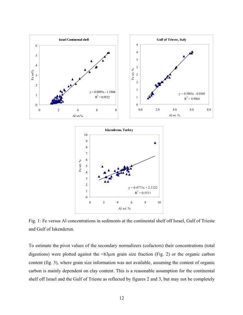
cofactors in the selected areas. For example, the deviations in the relationship between Fe and Al

concentrations in sediments at the continental shelf off Israel, Gulf of Trieste and Iskenderun are

presented in Fig. 1. Each region is characterized by different Fe/Al ratios or different slope in the

linear correlation. The slope in Iskenderun is almost half the slope at the continental shelf off

Israel. This change may reflect both the natural variations of the fine particle composition and

the local conditions for iron oxides precipitation.

11

Israel Continental shelf

y = 0.8895x - 1.1944R2 = 0.9522

0

1

2

3

4

5

6

0 2 4 6 8

Al wt.%

Fig. 1: Fe versus Al concentrations in sediments at the continental shelf off Israel, Gulf of Trieste

and Gulf of Iskenderun.

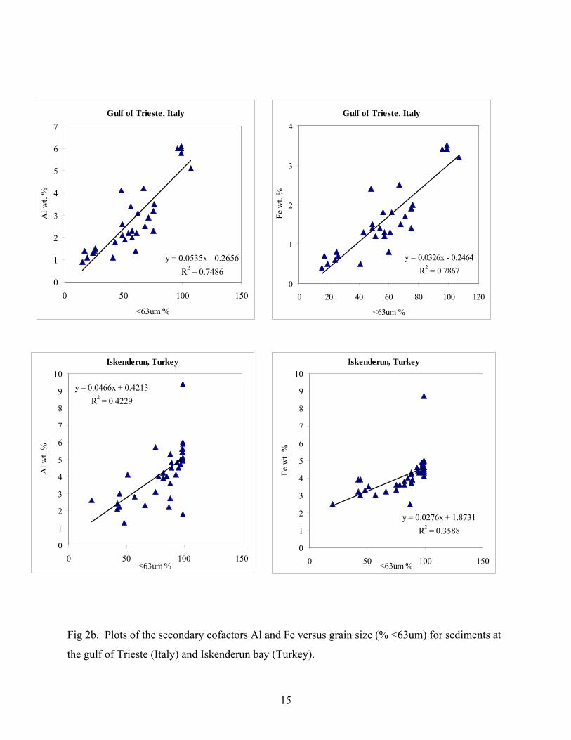
To estimate the pivot values of the secondary normalizers (cofactors) their concentrations (total

digestions) were plotted against the <63µm grain size fraction (Fig. 2) or the organic carbon

content (fig. 3), where grain size information was not available, assuming the content of organic

carbon is mainly dependent on clay content. This is a reasonable assumption for the continental

shelf off Israel and the Gulf of Trieste as reflected by figures 2 and 3, but may not be completely

Fe w

t%

Gulf of Trieste, Italy

y = 0.5903x - 0.0305R2 = 0.9864

0

1

1

2

2

3

3

4

4

0.0 2.0 4.0 6.0 8.0

Al wt. %

Fe w

t. %

Iskenderun, Turkey

y = 0.4771x + 2.1122R2 = 0.5511

0

1

2

3

4

5

6

7

8

9

10

0 2 4 6 8 1

Al wt. %

Fe w

t. %

0

12

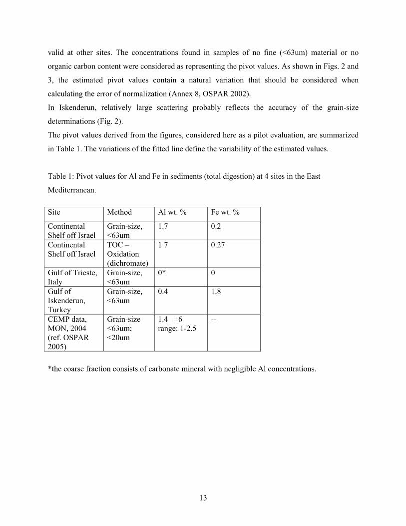
valid at other sites. The concentrations found in samples of no fine (<63um) material or no

organic carbon content were considered as representing the pivot values. As shown in Figs. 2 and

3, the estimated pivot values contain a natural variation that should be considered when

calculating the error of normalization (Annex 8, OSPAR 2002).

In Iskenderun, relatively large scattering probably reflects the accuracy of the grain-size

determinations (Fig. 2).

The pivot values derived from the figures, considered here as a pilot evaluation, are summarized

in Table 1. The variations of the fitted line define the variability of the estimated values.

Table 1: Pivot values for Al and Fe in sediments (total digestion) at 4 sites in the East

Mediterranean.

Site Method Al wt. % Fe wt. %

Continental Shelf off Israel

Grain-size, <63um

1.7 0.2

Continental Shelf off Israel

TOC – Oxidation (dichromate)

1.7 0.27

Gulf of Trieste, Italy

Grain-size, <63um

0*

0

Gulf of Iskenderun, Turkey

Grain-size, <63um

0.4 1.8

CEMP data, MON, 2004 (ref. OSPAR 2005)

Grain-size <63um; <20um

1.4 ±6 range: 1-2.5

--

*the coarse fraction consists of carbonate mineral with negligible Al concentrations.

13

Continental shelf off Israel Continental shelf off IsraelA

y = 0.0676x + 1.718R2 = 0.9873

0

1

2

3

4

5

6

7

8

0 20 40 60 80 100

y = 0.0607x + 0.2064R2 = 0.9903

0

1

2

3

4

5

6

0 20 40 60 80 10

<63um %Fe

wt.

%0

<63um %

Al w

t. %

Israel Shallow Water Israel Shallow WaterB

y = 0.413x + 1.6178R2 = 0.4602

0

0.5

1

1.5

2

2.5

0 0.5 1 1.5

y = 0.1833x + 0.1676R2 = 0.6141

0.0

0.1

0.2

0.3

0.4

0.5

0 0.5 1 1.5<63um %

Fe w

t.%

<63um %

Al w

t.%

Fig 2a. Plots of the secondary cofactors Al and Fe versus grain size (% <63um) for sediments at

the continental shelf off Israel (A) and shallow water sediments at water depths <10m (B).

14

Gulf of Trieste, Italy

y = 0.0535x - 0.2656R2 = 0.7486

0

1

2

3

4

5

6

7

0 50 100 150

<63um %

Al w

t. %

Gulf of Trieste, Italy

y = 0.0326x - 0.2464R2 = 0.7867

0

1

2

3

4

0 20 40 60 80 100 120

<63um %

Fe w

t. %

Iskenderun, Turkey

y = 0.0466x + 0.4213R2 = 0.4229

0

1

2

3

4

5

6

7

8

9

10

0 50 100 150<63um %

Al w

t. %

Iskenderun, Turkey

y = 0.0276x + 1.8731R2 = 0.3588

0

1

2

3

4

5

6

7

8

9

10

0 50 100 150<63um %

Fe w

t. %

Fig 2b. Plots of the secondary cofactors Al and Fe versus grain size (% <63um) for sediments at

the gulf of Trieste (Italy) and Iskenderun bay (Turkey).

15

Continental Shelf off Israel

y = 1.717x + 1.713R2 = 0.8217

0

1

2

3

4

5

6

7

0.0 0.5 1.0 1.5 2.0 2.5

Continental Shelf off Israel

y = 1.8346x + 0.2748R2 = 0.8273

0

1

2

3

4

5

0.0 0.5 1.0 1.5 2.0 2.5TOC wt.%

Fe w

t%

TOC wt.%

Al w

t%

Continental Shelf <63um - Greece 2004

y = 0.451x + 0.901R2 = 0.4216

0

1

2

3

4

5

6

7

0 2 4 6 8 1TOC wt.%

Fe w

t.%

0

Fig 3. Plot of the secondary cofactors Al and Fe versus TOC for sediments at the continental

shelf off Israel

16

Because heavy metals are present in the environment/sediments at different pollution levels it is

in principle problematic to define their pivot values applying the same approach as for the

secondary cofactors (intercepts of the regression lines). Such application may be valid for a non-

polluted (background) set of samples, which is difficult to define in the existing monitoring

datasets. Sediment cores representing a long-term record of pre-industrial period may serve as a

basis for such definitions, if representing the recent sedimentary composition.

In order to evaluate the pivot values of the heavy metals we examined those samples in which Al

concentrations were equal to or lower than the pivot value, assuming they closely represent pure

sand samples. Table 2 presents pivot values for a few heavy metals in sediments, based on the

datasets examined here and ICES data. For the data from the continental shelf off Israel, the

median values chosen as pivot values were compared to ranked metal concentrations (Fig. 4,

only Zn and Cd shown). The figure shows that only insignificant percent of the data is below the

estimated pivot values. Theoretically the pivot values are supposed to be the lowest possible

concentrations. However, too low values can lead to extrapolated or normalized values that are

too high.

The values presented in Table 2 for the East Mediterranean sites show extreme variability,

probably due to differences in sediment provinces. This aspect should be further studied at the

MED POL monitoring sites.

Table 2: Pivot values for heavy metals in sediment (total digestion).

Parameter Continental Shelf off Israel median; Al≤1.7%

Gulf of Trieste, Italy median; Al<1.4%

Iskenderun, Turkey Al=1.3%

ICES data OSPAR 2005; Al≤1.4%

median uncertainty

Cd 0.07 - - 0.04 0.02

Cr 11.6 - 118 5 5

Cu 1.1 - 19 1 1

Hg 0.004 - - 0.01 0.01

Ni 1.6 100 312 4 2

Pb 0.00 - 11 9 3

Zn 3.4 12 64 13 5

17

Continental Shelf off Israel (2002-4)

1

10

100

1000

1 6 11 16 21 26 31 36 41 46 51 56 61 66 71

Zn p

pm

0

1

2

3

4

5

6

Al %

ZnpivotAl

Continental Shelf off Israel (2002-4)

0.01

0.10

1.00

10.00

1 6 11 16 21 26 31 36 41 46 51 56 61 66

Cd

ppm

0

1

1

2

2

3

3

4

4

Al %

CdpivotAl

Fig. 4: Ranked (according content level) Zn and Cd concentrations in bulk sediments from the

continental shelf off Israel (2002-4), analyzed by total digestion. The open symbols indicate the

corresponding Al concentrations and the pivot value is marked by the triangle.

18

The normalized values of a monitoring dataset can be calculated based on equation (2) in

accordance to a standard sediment composition. The selection of the standard [reference]

sediment composition should take into consideration the range and average composition of the

studied sites, should have a chemical composition similar to that of the fine-grained component

and therefore result in a lower calculated uncertainty (OSPAR/JAMP 2002; Annex 8 and 9). The

proposed standard composition of Al for the data measured under JAMP is 5.8% (total digestion)

and 5% (strong digestion – HNO3 7N). It is impossible at this stage to recommend for a standard

sediment composition for the MED POL monitoring areas. It is recommended to perform a

comprehensive study to better define the bulk sediment major and trace chemical composition,

grain-size distribution and grain-size chemical composition. This will allow the derivation of

pivot values for primary, secondary and heavy metal components, mapping the range of

chemical composition in the whole MED POL monitoring sites and selecting the proper standard

sediment composition. This study can be performed on either archive sediment samples or on

new samples collected at the monitoring areas.

19

7. Recommendations

1. Analysis of bulk sediment (<2mm) is recommended since some areas contain

insignificant amounts of fine-silt and clays or variable mineralogical composition of the

sand fraction, and simplifies sample processing and potential artifacts that might change

the original composition.

2. A uniform digestion strength, preferably Total digestion is recommended for the

normalizers and several trace metals to obtain consistent extractions. However, for Cd

and Hg a strong partial digestion may be applied as well since in both digestion methods

a total extraction is achieved.

3. Aluminium (Al) determinations should be obligatory. If possible the determination of

additional normalizers is recommended (Fe and Li) to better assess basin-wide spatial and

temporal trends.

4. At this stage a gap of standardized datasets for the Mediterranean avoids the use of the

OSPAR chemical normalization approach. An interim approach might be to use the

approach presented in section 5.2 of the report.

5. A standard characteristic analysis should be performed for the monitoring areas to define:

i) grain-size analysis in order to achieve the relations between primary and secondary

normalizers; ii) define the heavy metal content in natural non-contaminated sand fraction;

iii) mapping the range of secondary normalizers (Al, Fe, Li) chemical composition across

the monitored areas to select the most proper standard sediment composition.

6. It is recommended to perform a retrospective analysis of Al in bulk archived samples to

better assess existing datasets.

7. After 4 above the errors associated with the normalization approach should be assessed.

20

8. References Ackerman F., 1980, A procedure for correcting grain size effect in heavy metal analysis of

estuaries and coastal sediments. Environment Technology Letters, 1: 518-527.

Aloupi M. and Angelidis M.O., 2001, Normalization to lithium for the assessment of metal

contamination on coastal sediment cores from the Aegean Sea, Greece. Marine Environmental

Research, 52: 1-12.

Barbanti A. and Bothner M.H., 1993, A procedure for partitioning bulk sediments into distinct

grain-size fractions for geochemical analysis. Environ. Geol., 21: 3-13.

Bertine K.K. and Goldberg E.D., 1977, History of heavy metal contamination in shallow coastal

sediments around Mitelene, Greece. International Journal of Environmental Analytical

Chemistry, 68: 281-293.

Carral E., Villares R., Puente X. and Carballeira A., 1995, Influence of watershed lithology on

heavy metal levels in estuarine sediments and organisms in Galicia (North-West Spain).

Marine Pollution Bulletin, 30: 604-608.

Blomqvist S., Larsson U. and Borg H., 1992, Heavy metal decrease in sediments of a Baltic Bay

following tertiary sewage treatment. Marine pollution Bulletin, 24: 258-266.

Covelli S. and Fontolan G., 1997, Application of a normalization procedure in determining

regional geochemical baselines. Environmental Geology, 30: 34-45

Dasklakis K.D. and O’Connor T.P., 1995, Normalization and elemental sediment contamination

in the coastal United States. Environmental Science and Technology, 29:470-477.

Din Z., 1992, Use of aluminum to normalize heavy-metal data from estuarine and coastal

sediments of Straits of Melaka. Marine Pollution Bulletin, 24: 484-491.

Dolenec T., Faganeli J. and Pirc S., 1998, Major, minor and trace elements in surficial sediments

from the open Adriatic Sea; a regional geochemical study. Geologia Croatica, 51: 59-73.

Emelyanov E.M., 1972, Principal types of Recent bottom sediments of the Mrditerranean Sea:

their mineralogy and geochemistry. In: Stanley D.J. (Ed.), The Mediterranean Sea: A Natural

Sedimentation Laboratory. Dowden, Hutchinson & Ross, Stroudsburg, Pennsylvania, pp. 355-

386.

Emelyanov E.M., Shimkus K.M. and Kuprin P.N., 1996, Unconsolidated bottom syrface

sediments of the Mediterranean and Black Seas. Intergovernmental Oceanographic Comission

(UNESCO) IBCM Geol.-Geoph. Sereies. Scale 1:1,000,000, 10 sheets, St. Peterburg, Russia.

21

Emelyanov E.M., Shimkus K.M. and Kuprin P.N., 2005, Explanatory notes to the IBCM-SED

map series Unconsolidated Sediments of the Mediterranean Sea and Black Sea. In: Hall J.K.,

Krashenninkov V.A., Hirsch F., Benjamini C. and Flexer A. (eds.), Geological Framework of

the Levant Vol. II: The Levantine Basin and Israel, pp. 183-214.

Ergin M., Kazan B. and Ediger V., 1996, Source and depositional controls on heavy metal

distribution in marine sediments of thr Gulf of Iskenderun, Eastern Mediterranean. Marine

Geology, 133: 223-239.

Grousset F.E., Quetel C.R., Thomas B., Donard O.F.X., Lambert C.E., Quillard F. and Monaco

A., 1995, Anthropogenic vs. lithogenic origins of trace elements (As, Cd, Pb, Rb, Sb, Sc, Sn,

Zn) in water column particles: northwestern Mediterranean Sea. Marine Chemistry, 48: 291-

310.

Hanson P., Evans D.W. and Colby D.R., 1993, Assessment of elemental contamination in

estuarine and coastal environments based on geochemical and statistical modeling of

sediments. Marine Environmental Research, 36: 237-266.

Herut B., Hornung H., Krom M.D., Kress N. and Cohen Y. (1993). Trace metals in shallow

sediments from the Mediterranean coastal region of Israel. Mar. Pollut. Bull., 26: 675-682.

Herut, B., Hornung, H., Kress, N., Krom, M.D. and Shirav, M. (1995). Trace metals in sediments

at the lower reaches of Mediterranean coastal rivers, Israel. Wat. Sci. Tech. 32: 239-246

JAMP/ICES guidelines for monitoring contaminants in sediments

Kersten M. and Smedes F., 2002, Normalization procedures for sediments contaminants in

spatial and temporal tren monitoring. J. Environ. Monit., 4: 109-115.

Krom M.D., Stanely J.D., Cliff R.A. and Woodward J.C., 2002, Nile River sediment fluctuations

over the past 7000 yr and their key role in sapropel development. Geology, 30: 71-74

Loring D.H., 1990, Lithium – a new approach for the granulometric noramalization of trace

metal data. Marine Chemistry, 29: 155-168.

Loring D.H and Rantala R.T.T., 1992, Manual for the geochemical analyses of marine sediments

and suspended particulate matter. Earth-Science Reviews, 32: 2350283, and 1995, Regional

Seas, Reference methods for marine pollution studies no. 63, United Nations Environment

Programme.

OSPAR/JAMP 2002. Guidelines for Monitoring Contaminants in Sediment. Ref. No. :2002-16

OSPAR 2005 Assessment of CEMP data.

22

Prohic E. and Juracic M., 1989, Heavy metals in sediments; problems concerning determination

of the anthropogenic influence; study in the Krka River estuary, eastern Adriatic Coast,

Yugoslavia. Environmental Geology and Water Sciences, 13: 145-151.

Prohic E. and Yuracic M., 1989, Heavy metals in sediments – problems concerning

determination of anthropogenic influence. Study in the Krka river estuary, eastern Adriatic

cost, Yugoslavia. Environmetal Geology and Water Science, 13: 145-151.

Roach A.C., 2005, Assessment of metals in sediments from Lake Macquarie, New South Wales,

Australia, using normalization models and sediment quality guidelines. Marine Environmental

Research, 59: 353-472.

Rule J.P., 1986, Assessment of trace element geochemistry of Hampton Roads Harbor and lower

Chesapeake Bay area sediments. Environmetal Geology and Water Science, 8: 209-219.

Schiff K.C. and Weisberg S.B., 1999, Iron as a reference element for determining trace metal

enrichment in Southern California costal shelf sediments. Marine Environmental Research,

48: 161-176.

Sinex S.A. and Wright D.A., 1988, Distribution of trace metals in the sediments and biota of

Chesapeake Bay. Marine Pollution Bulletin, 19: 425-431.

Vdovic N. and Juracic M., 1993, Sedimentological and surface characteristics of the northern

and central Adriatic sediments. Geologia Croatica, 46, 157-163.

23