reviews in computational chemistry · reviews in computational chemistry volume 20 edited by kenny...

Reviews inComputationalChemistryVolume 20

Reviews inComputationalChemistryVolume 20

Edited by

Kenny B. Lipkowitz, Raima Larter,and Thomas R. Cundari

Editor Emeritus

Donald B. Boyd

Copyright # 2004 by John Wiley & Sons, Inc. All rights reserved.

Published by John Wiley & Sons, Inc., Hoboken, New Jersey.Published simultaneously in Canada.

No part of this publication may be reproduced, stored in a retrieval system, or transmitted in any

form or by any means, electronic, mechanical, photocopying, recording, scanning, or otherwise,except as permitted under Section 107 or 108 of the 1976 United States Copyright Act, without

either the prior written permission of the Publisher, or authorization through payment of the

appropriate per-copy fee to the Copyright Clearance Center, Inc., 222 Rosewood Drive, Danvers,

MA 01923, 978-750-8400, fax 978-646-8600, or on the web at www.copyright.com. Requests tothe Publisher for permission should be addressed to the Permissions Department, John Wiley &

Sons, Inc., 111 River Street, Hoboken, NJ 07030, (201) 748-6011, fax (201) 748-6008.

Limit of Liability/Disclaimer of Warranty: While the publisher and author have used their bestefforts in preparing this book, they make no representations or warranties with respect to the

accuracy or completeness of the contents of this book and specifically disclaim any implied

warranties of merchantability or fitness for a particular purpose. No warranty may be created orextended by sales representatives or written sales materials. The advice and strategies contained

herein may not be suitable for your situation. You should consult with a professional where

appropriate. Neither the publisher nor the author shall be liable for any loss of profit or any

other commercial damages, including but not limited to special, incidental, consequential, orother damages.

For general information on our other products and services please contact our Customer Care

Department within the U.S. at 877-762-2974, outside the U.S. at 317-572-3993 or fax317-572-4002.

Wiley also publishes its books in a variety of electronic formats. Some content that appears inprint, however, may not be available in electronic format.

ISBN 0-471-44525-8

ISSN 1069-3599

Printed in the United States of America

10 9 8 7 6 5 4 3 2 1

Kenny B. LipkowitzDepartment of Chemistry

Ladd Hall 104

North Dakota State UniversityFargo, North Dakota 58105-5516, USA

[email protected]

Raima LarterDepartment of Chemistry

Indiana University-Purdue University

at Indianapolis,

402 North Blackford StreetIndianapolis, Indiana 46202-3274, USA

[email protected]

Thomas R. CundariDepartment of Chemistry

University of North Texas

Box 305070Denton, Texas 76203-5070, USA

[email protected]

Donald B. BoydDepartment of Chemistry

Indiana University-Purdue University

at Indianapolis

402 North Blackford StreetIndianapolis, Indiana 46202-3274, USA

[email protected]

Preface

Our goal over the years has been to provide tutorial-like reviews cover-ing all aspects of computational chemistry. In this, our twentieth volume, wepresent six chapters covering a diverse range of topics that are of interest tocomputational chemists. When one thinks of modern quantum chemical meth-ods there is a proclivity to think about molecular orbital theory (MOT). Thistheory has proved itself to be a useful theoretical tool that allows the compu-tation of energies, properties and, nowadays, dynamical aspects of molecularand supramolecular systems. Molecular orbital theory is, thus, valuable to theaverage bench chemist, but that bench chemist invariably wants to describechemical transformations to other chemists in a parlance based on the use ofresonance structures. So, an orbital localization scheme must be used to con-vert the fully delocalized MO results to a valence bond type representationthat is consonant with the chemist’s working language. One of the great meritsof valence bond theory (VBT) is its intuitive wave function. So, why not useVBT? If VBT is the lingua franca of most synthetic chemists, shouldn’t thosechemists be relying on the VBT method more than they now do, and, if they donot, how can those scientists learn about this quantum method? In Chapter 1,Professors Sason Shaik and Philippe Hiberty provide a detailed view of VBTvis-a-vis MOT, its demise, and then its renaissance; in short they give us a his-tory lesson about the topic. Following this, they outline the basic concepts ofVBT, describe the relationship between MOT and VBT, and provide insightsabout qualitative VBT. Comparisons with other quantum theories and withexperiment are made throughout. The VB state correlation method for electro-nic delocalization is defined and the controversial issue of what makes benzenehave its D6h structure is discussed. Aspects of photochemistry are then cov-ered. The spin Hamiltonian VBT and ab initio VB methods are also describedand reviewed, which provides a compelling historical account of VBT alongwith a tutorial and a review. It uses a parlance that is consistent with theway synthetic chemists naturally speak, and it contains insights concerningthe many uses of this vibrant field of quantum theory from two veteran VBtheorists.

Most chemists solving problems with quantum chemical tools typically workon a single potential energy surface. There are many chemical transformations,

v

however, where two or more potential energy surfaces need to be included todescribe properly the event that is taking place as is the case, for example, inphotoisomerizations. In many examples of photoexcitation, nonradiativeinternal conversion processes are followed that involve the decay of an excitedstate having the same multiplicity as the lower electronic state. In other pro-cesses, however, a nonradiative decay path can be followed where, say, a sing-let state can access a triplet state. How one goes about treating such changes inspin multiplicity is a daunting task, to both novice and seasoned computa-tional chemists alike. Professors Nikita Matsunaga and Shiro Koseki providea tutorial on the topic of modeling spin-forbidden reactions in Chapter 2. Theauthors describe for the novice the importance of the minimum energy cross-ing point (MEXP) and rationalize how spin–orbit coupling provides a mechan-ism for spin-forbidden reactions. An explanation of crossing probabilities, theFermi golden rule, and the Landau–Zener semiclassical approximation aregiven. Methodologies for obtaining spin–orbit matrix elements are presentedincluding, among others, the Klein–Gordon equation, the Dirac equation, theFoldy–Wouthuysen transformation, and the Breit–Pauli Hamiltonian. Withthis background the authors take the novice through a tutorial that explainshow to locate the MEXP. They describe programs available for modelingspin-forbidden reactions, and they then provide examples of such calculationson diatomic and polyatomic molecules.

Chapter 3 continues the theme of quantum chemistry and the excitedstate. In this chapter, Professor Stefan Grimme provides a tutorial explaininghow best to calculate electronic spectra of large molecules. Great care must betaken in the interpretation of electronic spectra because significant reorganiza-tion of the electronic and nuclear coordinates occurs upon excitation. Even formedium-sized molecules, the density of states in small energy regions canbe large, which leads to overlapping spectral features that are difficult toresolve (experimentally and theoretically). Other complications arise as well andthe novice computational chemist can become overwhelmed with the manydecisions that are needed to carry out the calculations in a meaningful manner.Professor Grimme addresses these challenges in this chapter by first introdu-cing and categorizing the types of electronic spectra and types of excited states,and then explaining the various theoretical aspects associated with simulatingelectronic spectra. In particular, excitation energies, transition moments, andvibrational structure are covered. Quantum chemical methods used for com-puting excited states of large molecules are highlighted with emphases on CI,perturbation methods, and time-dependent Hartree–Fock and density func-tional theory (DFT) methods. A set of recommendations that summarize themethods that can (and should) be used for calculating electronic spectra areprovided. Case studies on vertical absorption spectra, circular dichroism,and vibrational structure are then given. The author provides for the reader a basicunderstanding of which computational methodologies work while alerting thereader to those that do not. This tutorial imparts to the novice many years ofexperience by Professor Grimme about pitfalls to avoid.

vi Preface

In Chapter 4, Professor Raymond Kapral reviews the computationaltechniques used in simulating chemical waves and patterns produced by cer-tain chemical reactions such as the Belousov–Zhabotinsky reaction. He beginswith a brief discussion of the different length and time scales involved and anexplanation for the usual choice of a macroscopic modeling approach. Thefinite difference approach to modeling reaction-diffusion systems is nextreviewed and illustrated for a couple of simple model systems. One of these,the FitzHugh–Nagumo model, exhibits waves and patterns typical of excitablemedia. Kapral goes on to review other modeling approaches for excitablemedia, including the use of cellular automata and coupled map lattices.Finally, mesoscopic modeling techniques including Markov chain models forthe chemical dynamics of excitable systems are reviewed.

Chapter 5 by Professors Costel Sarbu and Horia Pop on Fuzzy Logiccomplements previous contributions to this series on Neural Networks(Volume 16) and Genetic Algorithms (Volume 10). Like the other artificialintelligence techniques, fuzzy logic has seen increasing usage in chemistry inthe past decade. Here, for the first time, the many different techniques thatfall within the arena of fuzzy logic are organized and presented. As delineatedby the authors, fuzzy logic is ideally suited for those areas in which impreciseor incomplete measurements are an issue. Its primary application has beenthe mining of large data sets. The fuzzy techniques discussed in this chapter areequally suited for achieving an effective reduction of the data in terms of eitherthe number of objects (by clustering of data) or a reduction in dimensionality.Additionally, cross-classification techniques make it possible to simultaneouslycluster data based on the objects and the characteristics that describe them. Inthis way, the characteristics that are responsible for two objects belonging tothe same (or different) chemical families can be probed directly. In either case,fuzzy methods afford the ability to probe relationships among the data that arenot apparent from traditional methods. An eclectic assortment of examplesfrom the literature of fuzzy logic in chemistry is provided, with special empha-sis on a subject near and dear to the heart of all chemists—the periodic table.Through the application of fuzzy logic, the chemical groups evident since thetime of Mendeleev emerge as the techniques evolve from being crisp to increas-ingly fuzzy. Professors Sarbu and Pop show how the different fuzzy classifica-tion schemes can be used to unearth relationships among the elements that arenot evident from a quick perusal of standard periodic tables. Other areas ofapplication include analysis of structural databases, toxicity profiling, struc-ture–activity relationships (SAR) and quantitative structure–activity relation-ships (QSAR). The chapter concludes with a discussion about interfacing offuzzy set theory with other soft computing techniques.

The final chapter in this volume (Chapter 6) covers a topic that has beenof major concern to computational chemists working in the pharmaceuticalindustry: Absorption, Metabolism, Distribution, Excretion, and Toxicology(ADME/Tox) of drugs. The authors of this chapter, Dr. Sean Ekins and Pro-fessor Peter Swaan, an industrial scientist and an academician, respectively,

Preface vii

provide a selective review of the current status of ADME/Tox covering severalintensely studied proteins. The common thread interconnecting these differentclasses of proteins is that the same computational techniques can be applied tounravel the intricacies of several individual systems. The authors begin bydescribing the concerted actions of transport and metabolism in mammalianphysiology. They then delineate the various approaches used to modelenzymes, transporters, channels, and receptors by describing, first, classicalQSAR methods and, then, pharmacophore models. Specific programs thatare used for the latter include Catalyst, DISCO, CoMFA, CoMSIA, GOLPE,and ALMOND, all of which are described in this chapter. The use of homol-ogy models are also explained. Following this introductory section on tech-niques, the authors review examples of ADME/Tox studies beginning withTransporter Systems, proceeding to Enzyme Systems, and then to Channelsand Receptors. Seventeen different case studies are presented to illustratehow the various modeling techniques have been used to evaluate ADME/Tox. A set of ‘‘Ten Commandments’’ that are applicable to many ADME/Tox properties as well as bioactivity models is given for the novice computa-tional chemist. A prognostication of future developments completes the chapter.

We invite our readers to visit the Reviews in Computational Chemistrywebsite at http://www.chem.ndsu.nodak.edu/RCC. It includes the author andsubject indexes, color graphics, errata, and other materials supplementing thechapters. We are delighted to report that the Google search engine (http://www.google.com/) ranks our website among the top hits in a search on theterm ‘‘computational chemistry’’. This search engine has become popularbecause it ranks hits in terms of their relevance and frequency of visits. Weare also pleased to report that the Institute for Scientific information, Inc.(ISI) rates the Reviews in Computational Chemistry book series in the top10 in the category of ‘‘general’’ journals and periodicals. The reason for theseaccomplishments rests firmly on the shoulders of the authors whom we havecontacted to provide the pedagogically driven reviews that have made thisongoing book series so popular. To those authors we are especially grateful.

We are also glad to note that our publisher has plans to make our mostrecent volumes available in an online form through Wiley InterScience. Pleasecheck the Web (http://www.interscience.wiley.com/onlinebooks) or [email protected] for the latest information. For readers who appreciatethe permanence and convenience of bound books, these will, of course, continue.

We thank the authors of this and previous volumes for their excellentchapters.

Kenny B. LipkowitzFargo, North Dakota

Raima LarterIndianapolis, IndianaThomas R. Cundari

Denton, TexasDecember 2003

viii Preface

Contents

1. Valence Bond Theory, Its History, Fundamentals,and Applications: A Primer 1Sason Shaik and Philippe C. Hiberty

Introduction 1A Story of Valence Bond Theory, Its Rivalry with Molecular

Orbital Theory, Its Demise, and Eventual Resurgence 2Roots of VB Theory 2Origins of MO Theory and the Roots of VB–MO Rivalry 5The ‘‘Dance’’ of Two Theories: One Is Up, the

Other Is Down 7Are the Failures of VB Theory Real Ones? 11Modern VB Theory: VB Theory Is Coming of Age 14

Basic VB Theory 16Writing and Representing VB Wave Functions 16The Relationship between MO and VB Wave Functions 22Formalism Using the Exact Hamiltonian 24Qualitative VB Theory 26Some Simple Formulas for Elementary Interactions 29

Insights of Qualitative VB Theory 34Are the ‘‘Failures’’ of VB Theory Real? 35Can VB Theory Bring New Insight into

Chemical Bonding? 42VB Diagrams for Chemical Reactivity 44

VBSCD: A General Model for Electronic Delocalization andIts Comparison with the Pseudo-Jahn–Teller Model 56

What Is the Driving Force, s or p, Responsible forthe D6h Geometry of Benzene? 57

VBSCD: The Twin-State Concept and Its Link toPhotochemical Reactivity 60

The Spin Hamiltonian VB Theory 65Theory 65Applications 67

Ab Initio VB Methods 69Orbital-Optimized Single-Configuration Methods 70Orbital-Optimized Multiconfiguration VB Methods 75

Prospective 84

ix

Appendix 84A.1 Expansion of MO Determinants in Terms of AO

Determinants 84A.2 Guidelines for VB Mixing 86A.3 Computing Mono-Determinantal VB Wave

Functions with Standard Ab Initio Programs 87Acknowledgments 87References 87

2. Modeling of Spin-Forbidden Reactions 101Nikita Matsunaga and Shiro Koseki

Overview of Reactions Requiring Two States 101Spin-Forbidden Reaction, Intersystem Crossing 103

Spin–Orbit Coupling as a Mechanism for Spin-ForbiddenReaction 105

General Considerations 105Atomic Spin–Orbit Coupling 106Molecular Spin–Orbit Coupling 107

Crossing Probability 110Fermi Golden Rule 110Landau–Zener Semiclassical Approximation 111

Methodologies for Obtaining Spin–Orbit Matrix Elements 111Electron Spin in Nonrelativistic Quantum Mechanics 112Klein–Gordon Equation 114Dirac Equation 115Foldy–Wouthuysen Transformation 117Breit–Pauli Hamiltonian 121Zeff Method 121Effective Core Potential-Based Method 123Model Core Potential-Based Method 124Douglas–Kroll Transformation 124

Potential Energy Surfaces 127Minimum Energy Crossing-Point Location 128

Available Programs for Modeling Spin-Forbidden Reactions 131Applications to Spin-Forbidden Reactions 132

Diatomic Molecules 132Polyatomic Molecules 134Phenyl Cation 137Norborene 138Conjugated Polymers 138CHð2�Þ þN2 ! HCNþNð4SÞ 139Molecular Properties 140Dynamical Aspects 141

Other Reactions 142

x Contents

Biological Chemistry 143Concluding Remarks 144Acknowledgments 145References 145

3. Calculation of the Electronic Spectra of Large Molecules 153Stefan Grimme

Introduction 153Types of Electronic Spectra 155Types of Excited States 158

Theory 162Excitation Energies 162Transition Moments 165Vibrational Structure 171Quantum Chemical Methods 175

Case Studies 188Vertical Absorption Spectra 188Circular Dichroism 200Vibrational Structure 204

Summary and Outlook 210Acknowledgments 211References 211

4. Simulating Chemical Waves and Patterns 219Raymond Kapral

Introduction 219Reaction–Diffusion Systems 221Cellular Automata 227Coupled Map Lattices 232Mesoscopic Models 237Summary 243References 244

5. Fuzzy Soft-Computing Methods and Their Applicationsin Chemistry 249Costel Sarbu and Horia F. Pop

Introduction 249Methods for Exploratory Data Analysis 250

Visualization of High-Dimensional Data 250Clustering Methods 251Projection Methods 252Linear Projection Methods 252Nonlinear Projection Methods 253

Artificial Neural Networks 254

Contents xi

Perceptron 254Multilayer Nets: Backpropagation 256Associative Memories: Hopfield Net 259Self-Organizing Map 260Properties 261Mathematical Characterization 262Relation between SOM and MDS 263Multiple Views of the SOM 263Other Architectures 263

Evolutionary Algorithms 264Genetic Algorithms 265

Canonical GA 265Evolution Strategies 266Evolutionary Programming 267

Fuzzy Sets and Fuzzy Logic 268Fuzzy Sets 269Fuzzy Logic 271Fuzzy Clustering 273Fuzzy Regression 274

Fuzzy Principal Component Analysis (FPCA) 278Fuzzy PCA (Optimizing the First Component) 278Fuzzy PCA (Nonorthogonal Procedure) 279Fuzzy PCA (Orthogonal) 280

Fuzzy Expert Systems (Fuzzy Controllers) 282Hybrid Systems 284

Combinations of Fuzzy Systems and Neutral Networks 284Fuzzy Genetic Algorithms 285Neuro-Genetic Systems 286

Fuzzy Characterization and Classification of the ChemicalElements and Their Properties 286

Hierarchical Fuzzy Classification of Chemical ElementsBased on Ten Physical Properties 288

Hierarchical Fuzzy Classification of Chemical ElementsBased on Ten Physical, Chemical, and Structural Properties 293

Fuzzy Hierarchical Cross-Classification of Chemical ElementsBased on Ten Physical Properties 297

Fuzzy Hierarchical Characteristics Clustering 304Fuzzy Horizontal Characteristics Clustering 305Characterization and Classification of Lanthanides and

Their Properties by PCA and FPCA 307Properties of Lanthanides Considered in This Study 308Classical PCA 310Fuzzy PCA 313Miscellaneous Applications of FPCA 317

xii Contents

Fuzzy Modeling of Environmental, SAR and QSAR Data 318Spectral Library Search and Spectra Interpretation 319Fuzzy Calibration of Analytical Methods and Fuzzy

Robust Estimation of Location and Spread 320Application of Fuzzy Neural Networks Systems in Chemistry 322Applications of Fuzzy Sets Theory and Fuzzy Logic in

Theoretical Chemistry 324Conclusions and Remarks 325References 325

6. Development of Computational Models for Enzymes,Transporters, Channels, and Receptors Relevant to ADME/Tox 333Sean Ekins and Peter W. Swaan

Introduction 333ADME/Tox Modeling: An Expansive Vision 333The Concerted Actions of Transport and Metabolism 335Metabolism 335Transporters 336

Approaches to Modeling Enzymes, Transporters, Channels,and Receptors 338

Classical QSAR 340Pharmacophore Models 341Homology Modeling 348

Transporter Modeling 348Applications of Transporters 349The Human Small Peptide Transporter, hPEPT1 350The Apical Sodium-Dependent Bile Acid Transporter 351P-Glycoprotein 353Vitamin Transporters 361Organic Cation Transporter 362Organic AnionTransporters 363Nucleoside Transporter 363Breast Cancer Resistance Protein 364Sodium Taurocholate Transporting Polypeptide 365

Enzymes 365Cytochrome P450 365Epoxide Hydrolase 370Monoamine Oxidase 370Flavin-Containing Monooxygenase 372Sulfotransferases 372Glucuronosyltransferases 373Glutathione S-transferases 375

Channels 376

Contents xiii

Human Ether-a-gogo Related Gene 376Receptors 382

Pregnane X-Receptor 382Constitutive Androstane Receptor 385

Future Developments 388Acknowledgments 392Abbreviations 393References 393

Author Index 417

Subject Index 443

xiv Contents

Contributors

Sean Ekins, GeneCo, 500 Renaissance Drive, Suite 106, St. Joseph, MI 49085,USA.(Electronic mail: [email protected])

Stefan Grimme, Theoretische Organische Chemie, Organisch-ChemischesInstitut der Universitat Munster, Correnstrasse 40, D-48149 Munster,Germany. (Electronic mail: [email protected])

Philippe C. Hiberty, Laboratoire de Chimie Physique, Groupe de ChimieTherique, Universite de Paris-Sud, 91405 Orsay, Cedex France.(Electronic mail: [email protected])

Raymond Kapral, Chemical Physics Theory Group, Department of Chemistry,University of Toronto, Toronto, Ontario M5S 3H6, Canada.(Electronic mail: [email protected])

Shiro Koseki, Department of Material Sciences, College of Integrated Arts andSciences, Osaka Prefecture University, 1-1, Gakuen-cho, Sakai 599-8531,Japan. (Electronic Mail: [email protected])

Nikita Matsunaga, Department of Chemistry and Biochemistry, Long IslandUniversity, 1 University Plaza, Brooklyn, NY 11201 USA.(Electronic mail: [email protected])

Horia F. Pop, Babes-Bolyai University, Faculty of Mathematics and ComputerScience, Department of Computer Science, 1, M. Kogalniceanu Street,RO-3400 Cluj-Napoca, Romania. (Electronic mail: [email protected])

Costel Sarbu, Babes-Bolyai University, Faculty of Chemistry and ChemicalEngineering, Department of Analytical Chemistry, 11 Arany Janos Street,RO-3400 Cluj-Napoca, Romania. (Electronic mail: [email protected])

xv

Sason Shaik, Department of Organic Chemistry and Lise Meitner-MinervaCenter for Computational Chemistry, Hebrew University, 91904 Jerusalem,Israel. (Electronic mail: [email protected])

Peter Swaan, Department of Pharmaceutical Sciences, University of Maryland,HSF2, 20 Penn Street, Baltimore, MD 21201 USA.(Electronic mail: [email protected])

xvi Contributors

Contributors toPrevious Volumes

Volume 1 (1990)

David Feller and Ernest R. Davidson, Basis Sets for Ab Initio MolecularOrbital Calculations and Intermolecular Interactions.

James J. P. Stewart, Semiempirical Molecular Orbital Methods.

Clifford E. Dykstra, Joseph D. Augspurger, Bernard Kirtman, and David J.Malik, Properties of Molecules by Direct Calculation.

Ernest L. Plummer, The Application of Quantitative Design Strategies inPesticide Design.

Peter C. Jurs, Chemometrics and Multivariate Analysis in Analytical Chemistry.

Yvonne C. Martin, Mark G. Bures, and Peter Willett, Searching Databases ofThree-Dimensional Structures.

Paul G. Mezey, Molecular Surfaces.

Terry P. Lybrand, Computer Simulation of Biomolecular Systems UsingMolecular Dynamics and Free Energy Perturbation Methods.

Donald B. Boyd, Aspects of Molecular Modeling.

Donald B. Boyd, Successes of Computer-Assisted Molecular Design.

Ernest R. Davidson, Perspectives on Ab Initio Calculations.

xvii

Volume 2 (1991)

Andrew R. Leach, A Survey of Methods for Searching the ConformationalSpace of Small and Medium-Sized Molecules.

John M. Troyer and Fred E. Cohen, Simplified Models for Understanding andPredicting Protein Structure.

J. Phillip Bowen and Norman L. Allinger, Molecular Mechanics: The Art andScience of Parameterization.

Uri Dinur and Arnold T. Hagler, New Approaches to Empirical Force Fields.

Steve Scheiner, Calculating the Properties of Hydrogen Bonds by Ab InitioMethods.

Donald E. Williams, Net Atomic Charge and Multipole Models for theAb Initio Molecular Electric Potential.

Peter Politzer and Jane S. Murray, Molecular Electrostatic Potentials andChemical Reactivity.

Michael C. Zerner, Semiempirical Molecular Orbital Methods.

Lowell H. Hall and Lemont B. Kier, The Molecular Connectivity Chi Indexesand Kappa Shape Indexes in Structure–Property Modeling.

I. B. Bersuker and A. S. Dimoglo, The Electron-Topological Approach to theQSAR Problem.

Donald B. Boyd, The Computational Chemistry Literature.

Volume 3 (1992)

Tamar Schlick, Optimization Methods in Computational Chemistry.

Harold A. Scheraga, Predicting Three-Dimensional Structures of Oligo-peptides.

Andrew E. Torda and Wilfred F. van Gunsteren, Molecular Modeling UsingNMR Data.

David F. V. Lewis, Computer-Assisted Methods in the Evaluation of ChemicalToxicity.

xviii Contributors to Previous Volumes

Volume 4 (1993)

Jerzy Cioslowski, Ab Initio Calculations on Large Molecules: Methodologyand Applications.

Michael L. McKee and Michael Page, Computing Reaction Pathways onMolecular Potential Energy Surfaces.

Robert M. Whitnell and Kent R. Wilson, Computational MolecularDynamics of Chemical Reactions in Solution.

Roger L. DeKock, Jeffry D. Madura, Frank Rioux, and Joseph Casanova,Computational Chemistry in the Undergraduate Curriculum.

Volume 5 (1994)

John D. Bolcer and Robert B. Hermann, The Development of ComputationalChemistry in the United States.

Rodney J. Bartlett and John F. Stanton, Applications of Post-Hartree–FockMethods: A Tutorial.

Steven M. Bachrach, Population Analysis and Electron Densities from Quan-tum Mechanics.

Jeffry D. Madura, Malcolm E. Davis, Michael K. Gilson, Rebecca C. Wade,Brock A. Luty, and J. Andrew McCammon, Biological Applications ofElectrostatic Calculations and Brownian Dynamics Simulations.

K. V. Damodaran and Kenneth M. Merz Jr., Computer Simulation of LipidSystems.

Jeffrey M. Blaney and J. Scott Dixon, Distance Geometry in Molecular Mod-eling.

Lisa M. Balbes, S. Wayne Mascarella, and Donald B. Boyd, A Perspective ofModern Methods in Computer-Aided Drug Design.

Volume 6 (1995)

Christopher J. Cramer and Donald G. Truhlar, Continuum Solvation Models:Classical and Quantum Mechanical Implementations.

Contributors to Previous Volumes xix

Clark R. Landis, Daniel M. Root, and Thomas Cleveland, MolecularMechanics Force Fields for Modeling Inorganic and OrganometallicCompounds.

Vassilios Galiatsatos, Computational Methods for Modeling Polymers: AnIntroduction.

Rick A. Kendall, Robert J. Harrison, Rik J. Littlefield, and Martyn F. Guest,High Performance Computing in Computational Chemistry: Methods andMachines.

Donald B. Boyd, Molecular Modeling Software in Use: Publication Trends.

Eiji �OOsawa and Kenny B. Lipkowitz, Appendix: Published Force FieldParameters.

Volume 7 (1996)

Geoffrey M. Downs and Peter Willett, Similarity Searching in Databases ofChemical Structures.

Andrew C. Good and Jonathan S. Mason, Three-Dimensional Structure Data-base Searches.

Jiali Gao, Methods and Applications of Combined Quantum Mechanical andMolecular Mechanical Potentials.

Libero J. Bartolotti and Ken Flurchick, An Introduction to Density FunctionalTheory.

Alain St-Amant, Density Functional Methods in Biomolecular Modeling.

Danya Yang and Arvi Rauk, The A Priori Calculation of Vibrational CircularDichroism Intensities.

Donald B. Boyd, Appendix: Compendium of Software for MolecularModeling.

Volume 8 (1996)

Zdenek Slanina, Shyi-Long Lee, and Chin-hui Yu, Computations in TreatingFullerenes and Carbon Aggregates.

xx Contributors to Previous Volumes

Gernot Frenking, Iris Antes, Marlis Bohme, Stefan Dapprich, Andreas W.Ehlers, Volker Jonas, Arndt Neuhaus, Michael Otto, Ralf Stegmann, AchimVeldkamp, and Sergei F. Vyboishchikov, Pseudopotential Calculations ofTransition Metal Compounds: Scope and Limitations.

Thomas R. Cundari, Michael T. Benson, M. Leigh Lutz, and Shaun O.Sommerer, Effective Core Potential Approaches to the Chemistry of theHeavier Elements.

Jan Almlof and Odd Gropen, Relativistic Effects in Chemistry.

Donald B. Chesnut, The Ab Initio Computation of Nuclear MagneticResonance Chemical Shielding.

Volume 9 (1996)

James R. Damewood, Jr., Peptide Mimetic Design with the Aid of Computa-tional Chemistry.

T. P. Straatsma, Free Energy by Molecular Simulation.

Robert J. Woods, The Application of Molecular Modeling Techniques to theDetermination of Oligosaccharide Solution Conformations.

Ingrid Pettersson and Tommy Liljefors, Molecular Mechanics CalculatedConformational Energies of Organic Molecules: A Comparison of ForceFields.

Gustavo A. Arteca, Molecular Shape Descriptors.

Volume 10 (1997)

Richard Judson, Genetic Algorithms and Their Use in Chemistry.

Eric C. Martin, David C. Spellmeyer, Roger E. Critchlow Jr., and Jeffrey M.Blaney, Does Combinatorial Chemistry Obviate Computer-Aided DrugDesign?

Robert Q. Topper, Visualizing Molecular Phase Space: Nonstatistical Effectsin Reaction Dynamics.

Raima Larter and Kenneth Showalter, Computational Studies in NonlinearDynamics.

Contributors to Previous Volumes xxi

Stephen J. Smith and Brian T. Sutcliffe, The Development of ComputationalChemistry in the United Kingdom.

Volume 11 (1997)

Mark A. Murcko, Recent Advances in Ligand Design Methods.

David E. Clark, Christopher W. Murray, and Jin Li, Current Issues inDe Novo Molecular Design.

Tudor I. Oprea and Chris L. Waller, Theoretical and Practical Aspects ofThree-Dimensional Quantitative Structure–Activity Relationships.

Giovanni Greco, Ettore Novellino, and Yvonne Connolly Martin, Approachesto Three-Dimensional Quantitative Structure–Activity Relationships.

Pierre-Alain Carrupt, Bernard Testa, and Patrick Gaillard, ComputationalApproaches to Lipophilicity: Methods and Applications.

Ganesan Ravishanker, Pascal Auffinger, David R. Langley, BhyravabhotlaJayaram, Matthew A. Young, and David L. Beveridge, Treatment of Counter-ions in Computer Simulations of DNA.

Donald B. Boyd, Appendix: Compendium of Software and Internet Tools forComputational Chemistry.

Volume 12 (1998)

Hagai Meirovitch, Calculation of the Free Energy and the Entropy ofMacromolecular Systems by Computer Simulation.

Ramzi Kutteh and T. P. Straatsma, Molecular Dynamics with GeneralHolonomic Constraints and Application to Internal Coordinate Constraints.

John C. Shelley and Daniel R. Berard, Computer Simulation of WaterPhysisorption at Metal–Water Interfaces.

Donald W. Brenner, Olga A. Shenderova, and Denis A. Areshkin, Quantum-Based Analytic Interatomic Forces and Materials Simulation.

Henry A. Kurtz and Douglas S. Dudis, Quantum Mechanical Methods forPredicting Nonlinear Optical Properties.

Chung F. Wong, Tom Thacher, and Herschel Rabitz, Sensitivity Analysis inBiomolecular Simulation.

xxii Contributors to Previous Volumes

Paul Verwer and Frank J. J. Leusen, Computer Simulation to Predict PossibleCrystal Polymorphs.

Jean-Louis Rivail and Bernard Maigret, Computational Chemistry in France:A Historical Survey.

Volume 13 (1999)

Thomas Bally and Weston Thatcher Borden, Calculations on Open-ShellMolecules: A Beginner’s Guide.

Neil R. Kestner and Jaime E. Combariza, Basis Set Superposition Errors:Theory and Practice.

James B. Anderson, Quantum Monte Carlo: Atoms, Molecules, Clusters,Liquids, and Solids.

Anders Wallqvist and Raymond D. Mountain, Molecular Models of Water:Derivation and Description.

James M. Briggs and Jan Antosiewicz, Simulation of pH-Dependent Proper-ties of Proteins Using Mesoscopic Models.

Harold E. Helson, Structure Diagram Generation.

Volume 14 (2000)

Michelle Miller Francl and Lisa Emily Chirlian, The Pluses and Minuses ofMapping Atomic Charges to Electrostatic Potentials.

T. Daniel Crawford and Henry F. Schaefer III, An Introduction to CoupledCluster Theory for Computational Chemists.

Bastiaan van de Graaf, Swie Lan Njo, and Konstantin S. Smirnov, Introduc-tion to Zeolite Modeling.

Sarah L. Price, Toward More Accurate Model Intermolecular Potentials forOrganic Molecules.

Christopher J. Mundy, Sundaram Balasubramanian, Ken Bagchi, MarkE. Tuckerman, Glenn J. Martyna, and Michael L. Klein, NonequilibriumMolecular Dynamics.

Donald B. Boyd and Kenny B. Lipkowitz, History of the Gordon ResearchConferences on Computational Chemistry.

Contributors to Previous Volumes xxiii

Mehran Jalaie and Kenny B. Lipkowitz, Appendix: Published Force FieldParameters for Molecular Mechanics, Molecular Dynamics, and Monte CarloSimulations.

Volume 15 (2000)

F. Matthias Bickelhaupt and Evert Jan Baerends, Kohn–Sham Density Func-tional Theory: Predicting and Understanding Chemistry.

Michael A. Robb, Marco Garavelli, Massimo Olivucci, and FernandoBernardi, A Computational Strategy for Organic Photochemistry.

Larry A. Curtiss, Paul C. Redfern, and David J. Frurip, Theoretical Methodsfor Computing Enthalpies of Formation of Gaseous Compounds.

Russell J. Boyd, The Development of Computational Chemistry in Canada.

Volume 16 (2000)

Richard A. Lewis, Stephen D. Pickett, and David E. Clark, Computer-AidedMolecular Diversity Analysis and Combinatorial Library Design.

Keith L. Peterson, Artificial Neural Networks and Their Use in Chemistry.

Jorg-Rudiger Hill, Clive M. Freeman, and Lalitha Subramanian, Use of ForceFields in Materials Modeling.

M. Rami Reddy, Mark D. Erion, and Atul Agarwal, Free Energy Calculations:Use and Limitations in Predicting Ligand Binding Affinities.

Volume 17 (2001)

Ingo Muegge and Matthias Rarey, Small Molecule Docking and Scoring.

Lutz P. Ehrlich and Rebecca C. Wade, Protein–Protein Docking.

Christel M. Marian, Spin–Orbit Coupling in Molecules.

Lemont B. Kier, Chao-Kun Cheng, and Paul G. Seybold, Cellular AutomataModels of Aqueous Solution Systems.

Kenny B. Lipkowitz and Donald B. Boyd, Appendix: Books Published on theTopics of Computational Chemistry.

xxiv Contributors to Previous Volumes

Volume 18 (2002)

Geoff M. Downs and John M. Barnard, Clustering Methods and Their Uses inComputational Chemistry.

Hans-Joachim Bohm and Martin Stahl, The Use of Scoring Functions in DrugDiscovery Applications.

Steven W. Rick and Steven J. Stuart, Potentials and Algorithms for Incorpor-ating Polarizability in Computer Simulations.

Dmitry V. Matyushov and Gregory A. Voth, New Developments in theTheoretical Description of Charge-Transfer Reactions in Condensed Phases.

George R. Famini and Leland Y. Wilson, Linear Free Energy RelationshipsUsing Quantum Mechanical Descriptors.

Sigrid D. Peyerimhoff, The Development of Computational Chemistry inGermany.

Donald B. Boyd and Kenny B. Lipkowitz, Appendix: Examination of theEmployment Environment for Computational Chemistry.

Volume 19 (2003)

Robert Q. Topper, David L. Freeman, Denise Bergin and KeirnanR. LaMarche, Computational Techniques and Strategies for Monte CarloThermodynamic Calculations, with Applications to Nanoclusters.

David E. Smith and Anthony D. J. Haymet, Computing Hydrophobicity.

Lipeng Sun and William L. Hase, Born–Oppenheimer Direct DynamicsClassical Trajectory Simulations.

Gene Lamm, The Poisson–Boltzmann Equation.

Contributors to Previous Volumes xxv

CHAPTER 1

Valence Bond Theory, Its History,Fundamentals, and Applications:A Primera

Sason Shaik* and Philippe C. Hiberty{

*Department of Organic Chemistry and Lise Meitner-MinervaCenter for Computational Chemistry, Hebrew University 91904Jerusalem, Israel{Laboratoire de Chimie Physique, Groupe de Chimie Theorique,Universite de Paris-Sud, 91405 Orsay Cedex, France

INTRODUCTION

The new quantum mechanics of Heisenberg and Schrodinger have pro-vided chemistry with two general theories of bonding: valence bond (VB)theory and molecular orbital (MO) theory. The two were developed at aboutthe same time, but quickly diverged into rival schools that have competed,sometimes fervently, in charting the mental map and epistemology of chemis-try. Until the mid-1950s, VB theory dominated chemistry; then, MO theorytook over while VB theory fell into disrepute and was soon almost completelyabandoned. From the 1980s onward, VB theory made a strong comeback andhas ever since been enjoying a renaissance both in qualitative applications of

Reviews in Computational Chemistry, Volume 20edited by Kenny B. Lipkowitz, Raima Larter, and Thomas R. Cundari

ISBN 0-471-44525-8 Copyright � 2004 John Wiley & Sons, Inc.

aThis review is dedicated to Roald Hoffmann—A great teacher and a friend.

1

the theory and the development of new methods for computational implemen-tation.1

One of the great merits of VB theory is its visually intuitive wave func-tion, expressed as a linear combination of chemically meaningful structures. Itis this feature that made VB theory so popular in the 1930s–1950s, and, iro-nically, it is the same feature that accounts for its temporary demise (and ulti-mate resurgence). The comeback of this theory is, therefore, an importantdevelopment. A review of VB theory that highlights its insight into chemicalproblems and discusses some of its state-of-the-art methodologies is timely.

This chapter is aimed at the nonexpert and designed as a tutorial forfaculty and students who would like to teach and use VB theory, but possessonly a basic knowledge of quantum chemistry. As such, an important focus ofthe chapter will be the qualitative wisdom of the theory and the way it appliesto problems of bonding and reactivity. This part will draw on material dis-cussed in previous works by the authors. Another focus of the chapter willbe on the main methods available today for ab initio VB calculations. How-ever, much important work of a technical nature will, by necessity, be left out.Some of this work (but certainly not all) is covered in a recent monograph onVB theory.1

A STORY OF VALENCE BOND THEORY, ITSRIVALRY WITH MOLECULAR ORBITAL THEORY,ITS DEMISE, AND EVENTUAL RESURGENCE

Since VB has achieved a reputation in some circles as an obsolete theory,it is important to give a short historical account of its development includingthe rivalry of VB and MO theory, the fall from favor of VB theory, and thereasons for the dominance of MO theory and the eventual resurgence of VBtheory. Part of the historical review is based on material from the fascinatinghistorical accounts of Servos2 and Brush.3,4 Other parts are not published his-torical accounts, but rational analyses of historical events, reflecting our ownopinions and comments made by colleagues.

Roots of VB Theory

The roots of VB theory in chemistry can be traced to the famous paper ofLewis ‘‘The Atom and The Molecule’’,5 which introduces the notions of elec-tron-pair bonding and the octet rule.2 Lewis was seeking an understanding ofweak and strong electrolytes in solution, and this interest led him to formulatethe concept of the chemical bond as an intrinsic property of the molecule thatvaries between the covalent (shared-pair) and ionic situations. Lewis’ paperpredated the introduction of quantum mechanics by 11 years, and constitutes

2 VB Theory, Its History, Fundamentals, and Applications

the first formulation of bonding in terms of the covalent–ionic classification. Itis still taught today and provides the foundation for the subsequent construc-tion and generalization of VB theory. Lewis’ work eventually had its greatestimpact through the work of Langmuir who articulated Lewis’ model andapplied it across the periodic table.6

The overwhelming support of the chemistry community for Lewis’ ideathat electron pairs play a fundamental role in bonding provided an excitingagenda for research directed at understanding the mechanism by which anelectron pair could constitute a bond. The nature of this mechanism remained,however, a mystery until 1927 when Heitler and London traveled to Zurich towork with Schrodinger. In the summer of the same year they published theirseminal paper, Interaction between Neutral Atoms and Homopolar Bind-ing,7,8 in which they showed that the bonding in H2 can be accounted forby the wave function drawn in 1, in Scheme 1. This wave function is a super-

position of two covalent situations in which one electron is in the spin up con-figuration (a spin), while the other is spin down (b spin) [form (a)], and viceversa in the second form (b). Thus, the bonding in H2 was found to originate inthe quantum mechanical ‘‘resonance’’ between the two situations of spinarrangement required to form a singlet electron pair. This ‘‘resonance energy’’accounted for �75% of the total bonding of the molecule, and thereby sug-gested that the wave function in 1, which is referred to henceforth as theHL (Heitler–London) wave function, can describe the chemical bonding in asatisfactory manner. This ‘‘resonance origin’’ of bonding was a remarkableinsight of the new quantum theory, since prior to that time it was not obvioushow two neutral species could bond.

The notion of resonance was based on the work of Heisenberg,9 whoshowed that, since electrons are indistinguishable particles then, for a two-electron system, with two quantum numbers n and m, there exist two wave

Scheme 1

A Story of Valence Bond Theory 3

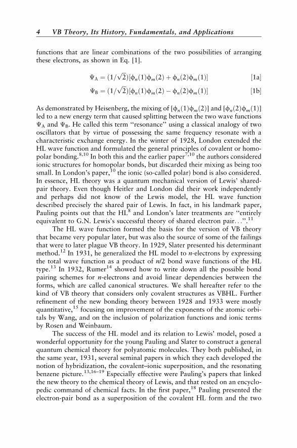
functions that are linear combinations of the two possibilities of arrangingthese electrons, as shown in Eq. [1].

�A ¼ ð1=ffiffiffi2pÞ½fnð1Þfmð2Þ þ fnð2Þfmð1Þ� ½1a�

�B ¼ ð1=ffiffiffi2pÞ½fnð1Þfmð2Þ fnð2Þfmð1Þ� ½1b�

As demonstrated by Heisenberg, the mixing of [fnð1Þfmð2Þ] and [fnð2Þfmð1Þ]led to a new energy term that caused splitting between the two wave functions�A and �B. He called this term ‘‘resonance’’ using a classical analogy of twooscillators that by virtue of possessing the same frequency resonate with acharacteristic exchange energy. In the winter of 1928, London extended theHL wave function and formulated the general principles of covalent or homo-polar bonding.8,10 In both this and the earlier paper7,10 the authors consideredionic structures for homopolar bonds, but discarded their mixing as being toosmall. In London’s paper,10 the ionic (so-called polar) bond is also considered.In essence, HL theory was a quantum mechanical version of Lewis’ shared-pair theory. Even though Heitler and London did their work independentlyand perhaps did not know of the Lewis model, the HL wave functiondescribed precisely the shared pair of Lewis. In fact, in his landmark paper,Pauling points out that the HL8 and London’s later treatments are ‘‘entirelyequivalent to G.N. Lewis’s successful theory of shared electron pair. . .’’.11

The HL wave function formed the basis for the version of VB theorythat became very popular later, but was also the source of some of the failingsthat were to later plague VB theory. In 1929, Slater presented his determinantmethod.12 In 1931, he generalized the HL model to n-electrons by expressingthe total wave function as a product of n/2 bond wave functions of the HLtype.13 In 1932, Rumer14 showed how to write down all the possible bondpairing schemes for n-electrons and avoid linear dependencies between theforms, which are called canonical structures. We shall hereafter refer to thekind of VB theory that considers only covalent structures as VBHL. Furtherrefinement of the new bonding theory between 1928 and 1933 were mostlyquantitative,15 focusing on improvement of the exponents of the atomic orbi-tals by Wang, and on the inclusion of polarization functions and ionic termsby Rosen and Weinbaum.

The success of the HL model and its relation to Lewis’ model, posed awonderful opportunity for the young Pauling and Slater to construct a generalquantum chemical theory for polyatomic molecules. They both published, inthe same year, 1931, several seminal papers in which they each developed thenotion of hybridization, the covalent–ionic superposition, and the resonatingbenzene picture.13,16–19 Especially effective were Pauling’s papers that linkedthe new theory to the chemical theory of Lewis, and that rested on an encyclo-pedic command of chemical facts. In the first paper,18 Pauling presented theelectron-pair bond as a superposition of the covalent HL form and the two


possible ionic forms of the bond, as shown in 2 in Scheme 1, and discussed thetransition from covalent to ionic bonding. He then developed the notion ofhybridization and discussed molecular geometries and bond angles in a varietyof molecules, ranging from organic to transition metal compounds. For the lat-ter compounds, he also discussed the magnetic moments in terms of theunpaired spins. In the second paper,19 Pauling addressed bonding in moleculeslike diborane, and odd-electron bonds as in the ion molecule Hþ2 and dioxy-gen, O2, which Pauling represented as having two three-electron bonds, asshown in 3 in Scheme 1. These two papers were followed by more papers,all published during 1931–1933 in the Journal of the American ChemicalSociety, and collectively entitled ‘‘The Nature of the Chemical Bond’’. Thisseries of papers allowed one to describe any bond in any molecule, and culmi-nated in Pauling’s famous monograph20 in which all structural chemistry ofthe time was treated in terms of the covalent–ionic superposition theory, reso-nance theory, and hybridization theory. The book, published in 1939, wasdedicated to G.N. Lewis, and, in fact, the 1916 paper of Lewis is the onlyreference cited in the preface to the first edition. Valence bond theory is, inPauling’s view, a quantum chemical version of Lewis’ theory of valence. InPauling’s work, the long sought for Allgemeine Chemie (Generalized Chemis-try) of Ostwald was, thus, finally found.2

Origins of MO Theory and the Roots of VB–MO Rivalry

At the same time that Slater and Pauling were developing their VBtheory,17 Mulliken21–24 and Hund25,26 were working on an alternative approach,which would eventually be called molecular orbital (MO) theory. The actualterm (MO theory) does not appear until 1932, but the roots of the method canbe traced to earlier papers from 1928,21 in which both Hund and Mullikenmade spectral and quantum number assignments of electrons in molecules,based on correlation diagrams of separated to united atoms. According toBrush,3 the first person to write a wave function for a molecular orbital wasLennard-Jones in 1929, in his treatment of diatomic molecules. In this paper,Lennard-Jones shows with facility that the O2 molecule is paramagnetic, andmentions that the VBHL method runs into difficulties with this molecule.27 InMO theory, the electrons in a molecule occupy delocalized orbitals made fromlinear combinations of atomic orbitals (LCAO). Drawing 4, Scheme 1, showsthe molecular orbitals of the H2 molecule; the delocalized sg MO should becontrasted with the localized HL description in 1.

The work of Huckel in the early 1930s initially received a chilly recep-tion,28 but eventually Huckel’s work gave MO theory an impetus and devel-oped into a successful and widely applicable tool. In 1930, Huckel usedLennard-Jones’ MO ideas on O2, applied it to CX (X¼C, N, O) doublebonds and suggested the concept of s–p separation.29 With this novel treat-ment, Huckel ascribed the restricted rotation in ethylene to the p-type orbital.


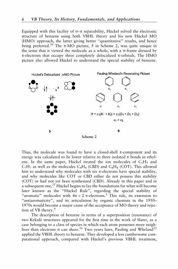
Equipped with this facility of s–p separability, Huckel solved the electronicstructure of benzene using both VBHL theory and his new Huckel MO(HMO) approach, the latter giving better ‘‘quantitative’’ results, and hencebeing preferred.30 The p-MO picture, 5 in Scheme 2, was quite unique inthe sense that it viewed the molecule as a whole, with a s-frame dressed byp-electrons that occupy three completely delocalized p-orbitals. The HMOpicture also allowed Huckel to understand the special stability of benzene.

Thus, the molecule was found to have a closed-shell p-component and itsenergy was calculated to be lower relative to three isolated p bonds in ethyl-ene. In the same paper, Huckel treated the ion molecules of C5H5 andC7H7 as well as the molecules C4H4 (CBD) and C8H8 (COT). This allowedhim to understand why molecules with six p-electrons have special stability,and why molecules like COT or CBD either do not possess this stability(COT) or had not yet been synthesized (CBD). Already in this paper and ina subsequent one,31 Huckel begins to lay the foundations for what will becomelater known as the ‘‘Huckel Rule’’, regarding the special stability of‘‘aromatic’’ molecules with 4nþ 2 p-electrons.3 This rule, its extension to‘‘antiaromaticity’’, and its articulation by organic chemists in the 1950–1970s would become a major cause of the acceptance of MO theory and rejec-tion of VB theory.4

The description of benzene in terms of a superposition (resonance) oftwo Kekule structures appeared for the first time in the work of Slater, as acase belonging to a class of species in which each atom possesses more neigh-bors than electrons it can share.16 Two years later, Pauling and Wheland32

applied the VBHL theory to benzene. They developed a less cumbersome com-putational approach, compared with Huckel’s previous VBHL treatment,

Scheme 2


using the five canonical structures, in 6 in Scheme 2, and approximated thematrix elements between the structures by retaining only close neighbor reso-nance interactions. Their approach allowed them to extend the treatment tonaphthalene and to a great variety of other species. Thus, in the VBHLapproach, benzene is described as a ‘‘resonance hybrid’’ of the two Kekulestructures and the three Dewar structures; the latter had already appearedbefore in Ingold’s idea of mesomerism. In his book, published for the firsttime in 1944, Wheland explains the resonance hybrid with the biological ana-logy of mule¼ donkeyþ horse.33 The pictorial representation of the wavefunction, the link to Kekule’s oscillation hypothesis, and the connection toIngold’s mesomerism, all of which were known to chemists, made theVBHL representation very popular among practicing chemists.

With these two seemingly different treatments of benzene, the chemicalcommunity was faced with two alternative descriptions of one of its molecularicons. Thus began the VB–MO rivalry that continues to the twenty-firstcentury. The VB–MO rivalry involved many prominent chemists (to mentionbut a few names, Mulliken, Huckel, J. Mayer, Robinson, Lapworth, Ingold,Sidgwick, Lucas, Bartlett, Dewar, Longuet-Higgins, Coulson, Roberts, Win-stein, Brown, etc.). A detailed and interesting account of the nature of this riv-alry and the major players can be found in the treatment of Brush.3,4

Interestingly, as early as the 1930s, Slater17 and van Vleck and Sherman34 sta-ted that since the two methods ultimately converge, it is senseless to quibbleabout the issue of which one is better. Unfortunately, however, this rationalattitude does not seem to have made much of an impression.

The ‘‘Dance’’ of Two Theories: One Is Up,the Other Is Down

By the end of World War II, Pauling’s resonance theory had becomewidely accepted while most practicing chemists ignored HMO and MO theo-ries. The reasons for this are analyzed by Brush.3 Mulliken suggested thatthe success of VB theory was due to Pauling’s skill as a propagandist. Accord-ing to Hager (a Pauling biographer) VB theory won out in the 1930s becauseof Pauling’s communication skills. However, the most important reason for itsdominance is the direct lineage of VB-resonance theory to the structural con-cepts of chemistry dating from the days of Kekule. Pauling himself emphasizedthat his VB theory is a natural evolution of chemical experience, and that itemerges directly from the concept of the chemical bond. This has made VB-resonance theory appear intuitive and ‘‘chemically correct’’. Another greatpromoter of VB-resonance theory was Ingold who saw in it a quantum chemi-cal version of his own ‘‘mesomerism’’ concept (according to Brush, the termsresonance and mesomerism entered chemical vocabulary at the same time, dueto Ingold’s assimilation of VB-resonance theory; see Brush,3 p. 57). Anothervery important reason for the early acceptance of VB theory is the facile


qualitative application of this theory to all known structural chemistry of thetime (in Pauling’s book20) and to a variety of problems in organic chemistry (inWheland’s book33). The combination of an easily applicable general theoryand its good fit to experiment, created a rare credibility nexus. By contrast,MO theory seemed diametrically opposed to everything chemists had thoughtwas true about the nature of the chemical bond. Even Mulliken admitted thatMO theory departs from ‘‘chemical ideology’’ (see Brush,3 p. 51). And to com-plete this sad state of affairs, in this early period MO theory offered no visualrepresentation to compete with the resonance hybrid representation ofVB-resonance theory. For all these reasons, by the end of World War II,VB-resonance theory dominated the epistemology of chemists.

By the mid-1950s, the tide had started a slow turn in favor of MOtheory, a shift that gained momentum through the mid-1960s. What causedthe shift is a combination of factors, of which the following two may be deci-sive. First, there were the many successes of MO theory: the experimental ver-ification of Huckel’s rules;28 the construction of intuitive MO theories andtheir wide applicability for rationalization of structures (e.g., Walsh diagrams)and spectra [electronic and electron spin resonance (ESR)]; the highly success-ful predictive application of MO theory in chemical reactivity; the instantrationalization of the bonding in newly discovered exotic molecules like ferro-cene,35 for which the VB theory description was cumbersome; and the devel-opment of widely applicable MO-based computational techniques (e.g.,extended Huckel and semiempirical programs). The second reason, on theother side, is that VB theory, in chemistry, suffered a detrimental conceptualarrest that crippled the predictive ability of the theory and started to lead to anaccumulation of ‘‘failures’’. Unlike its fresh exciting beginning, in its frozenform of the 1950–1960s, VB theory ceased to guide experimental chemiststo new experiments. This lack of utility ultimately led to the complete victoryof MO theory. However, the MO victory over VB theory was restricted toresonance theory and other simplified versions of VB theory, not VB theoryitself. In fact, by this time, the true VB theory was hardly being practiced any-more in the mainstream chemical community.

One of the major registered ‘‘failures’’ of VB theory is associated withthe dioxygen molecule, O2. Application of the Pauling–Lewis recipe of hybri-dization and bond pairing to rationalize and predict the electronic structure ofmolecules fails to predict the paramagneticity of O2. By contrast, MO theoryreveals this paramagneticity instantaneously.27 Even though VB theory doesnot really fail with O2, and Pauling himself preferred, without reasoningwhy, to describe it in terms of three-electron bonds (3 in Scheme 1) in his earlypapers19 (see also Wheland’s description on p. 39 of his book33), this ‘‘failure’’of Pauling’s recipe has tainted VB theory and become a fixture of the commonchemical wisdom (see Brush3 p. 49, footnote 112).

A second example concerns the VB treatments of CBD and COT. Theuse of VBHL theory leads to an incorrect prediction that the resonance energy


of CBD should be as large as or even larger than that of benzene. The facts(that CBD had not yet been made and that COT exhibited no special stability)favored HMO theory. Another impressive success of HMO theory was theprediction that due to the degenerate set of singly occupied MOs, squareCBD should distort to a rectangular structure, which provided a theoreticalexplanation for the ubiquitous phenomena of Jahn-Teller and pseudo-Jahn-Teller effects, amply observed by the community of spectroscopists. Whelandanalyzed the CBD problem early on, and his analysis pointed out that inclu-sion of ionic structures would probably change the VB predictions and makethem identical to MO.33,36,37 Craig showed that VBHL theory in fact correctlyassigns the ground state of CBD, by contrast to HMO theory.38,39 Despite thismixed bag of predictions on properties of CBD, by VBHL or HMO, anddespite the fact that modern VB theory has subsequently demonstrated uniqueand novel insight into the problems of benzene, CBD and their isoelectronicspecies, the early stamp of the CBD story as a failure of VB theory still persists.

The increasing interest of chemists in large molecules as of the late 1940sstarted making VB theory impractical, compared with the emerging semiem-pirical MO methods that allowed the treatment of larger and larger molecules.A great advantage of semiempirical MO calculations was the ability to calcu-late bond lengths and angles rather than assume them as in VB theory.4 Skillfulcommunicators like Longuet–Higgins, Coulson, and Dewar were among theleading MO proponents, and they handled MO theory in a visualizable man-ner, which had been sorely missing before. In 1951, Coulson addressed theRoyal Society Meeting and expressed his opinion that despite the great successof VB theory, it had no good theoretical basis; it was just a semiempiricalmethod, he said, of little use for more accurate calculations.40 In 1949,Dewar’s monograph, Electronic Theory of Organic Chemistry,41 summarizedthe faults of resonance theory, as being cumbersome, inaccurate, and tooloose: ‘‘it can be played happily by almost anyone without any knowledgeof the underlying principles involved’’. In 1952, Coulson published his bookValence,42 which did for MO theory, at least in part, what Pauling’s book20

had done much earlier for VB theory. In 1960, Mulliken won the Nobel Prizeand Platt wrote, ‘‘MO is now used far more widely, and simplified versions ofit are being taught to college freshmen and even to high school students’’.43

Indeed, many communities took to MO theory due to its proven portabilityand successful predictions.

A decisive defeat was dealt to VB theory when organic chemists werefinally able to synthesize transient molecules and establish the stability pat-terns of C8H2

8 , C5H;þ5 , C3Hþ;3 and C7Hþ;7 during the 1950–1960s.3,4,28

The results, which followed Huckel’s rules, convinced most of the organic che-mists that MO theory was right, while VBHL and resonance theories werewrong. From 1960–1978, C4H4 was made, and its structure and propertiesas determined by MO theory challenged initial experimental determinationof a square structure.3,4 The syntheses of nonbenzenoid aromatic compounds


like azulene, tropone, and so on, further established Huckel’s rules, and high-lighted the failure of resonance theory.28 This era in organic chemistry markeda decisive down-fall of VB theory.

In 1960, the 3rd edition of Pauling’s book was published,20 and althoughit was still spellbinding for chemists, it contained errors and omissions. Forexample, in the discussion of electron deficient boranes, Pauling describesthe molecule B12H12 instead of B12H2

12 (Pauling,20 p. 378); another exampleis a very cumbersome description of ferrocene and analogous compounds (onpp. 385–392), for which MO theory presented simple and appealing descrip-tions. These and other problems in the book, as well as the neglect of then-known species like C5H;þ5 , C3Hþ;3 , and C7Hþ;7 , reflected the situationthat, unlike MO theory, VB theory did not have a useful Aufbau principlethat could predict reliably the dependence of molecular stability on the num-ber of electrons. As we have already pointed out, the conceptual developmentof VB theory had been arrested since the 1950s, in part due to the insistence ofPauling himself that resonance theory was sufficient to deal with most pro-blems (see, e.g., p. 283 in Brush4). Sadly, the creator himself contributed tothe downfall of his own brainchild.

In 1952, Fukui published his Frontier MO theory,44 which went initiallyunnoticed. In 1965, Woodward and Hoffmann published their principle ofconservation of orbital symmetry, and applied it to all pericyclic chemicalreactions. The immense success of these rules45 renewed interest in Fukui’sapproach and together formed a new MO-based framework of thought forchemical reactivity (called, e.g., ‘‘giant steps forward in chemical theory’’ inMorrison and Boyd, pp. 934, 939, 1201, and 1203). This success of MOtheory dealt a severe blow to VB theory. In this area too, despite the early cal-culations of the Diels–Alder and 2þ 2 cycloaddition reactions by Evans,46 VBtheory missed making an impact, in part at least because of its blind adherenceto simple resonance theory.28 All the subsequent VB derivations of the rules(e.g., by Oosterhoff in Ref. 90) were ‘‘after the fact’’ and failed to reestablishthe status of VB theory.

The development of photoelectron spectroscopy (PES) and its applica-tion to molecules in the 1970s, in the hands of Heilbronner, showed that spec-tra could be easily interpreted if one assumes that electrons occupy delocalizedmolecular orbitals.47,48 This further strengthened the case for MO theory.Moreover, this served to lessen the case for VB theory, because it describeselectron pairs that occupy localized bond orbitals. A frequent example ofthis ‘‘failure’’ of VB theory is the PES of methane, which shows two differentionization peaks. These peaks correspond to the a1 and t2 MOs, but not tothe four CH bond orbitals in Pauling’s hybridization theory (see a recentpaper on a similar issue49). With these and similar types of arguments VBtheory has eventually fallen into a state of disrepute and become known, atleast when the authors were students, either as a ‘‘wrong theory’’ or even a‘‘dead theory’’.


The late 1960s and early 1970s mark the era of mainframe computing.By contrast to VB theory, which is difficult to implement computationally (dueto the non-orthogonality of orbitals), MO theory could be easily implemented(even GVB was implemented through an MO-based formalism—see later). Inthe early 1970s, Pople and co-workers developed the GAUSSIAN70 packagethat uses ‘‘ab initio MO theory’’ with no approximations other than the choiceof basis set. Sometime later density functional theory made a spectacular entryinto chemistry. Suddenly, it became possible to calculate real molecules, and toprobe their properties with increasing accuracy. This new and user-friendlytool created a subdiscipline of ‘‘computational chemists’’ who explore themolecular world with the GAUSSIAN series and many other packages thatsprouted alongside the dominant one. Calculations continuously reveal‘‘more failures’’ of Pauling’s VB theory, for example, the unimportance of3d orbitals in bonding of main group elements, namely, the ‘‘verification’’of three-center bonding. Leading textbooks hardly include VB theory any-more, and when they do, they misrepresent the theory.50,51 Advanced quan-tum chemistry courses teach MO theory regularly, but books that teach VBtheory are virtually nonexistent. The development of user friendly ab initioMO-based software and the lack of similar VB software seem to have putthe last nail in the coffin of VB theory and substantiated MO theory as theonly legitimate chemical theory of bonding.

Nevertheless, despite this seemingly final judgment and the obituariesshowered on VB theory in textbooks and in public opinion, the theory hasnever really died. Due to its close affinity to chemistry and utmost clarity, ithas remained an integral part of the thought process of many chemists, evenamong proponents of MO theory (see comment by Hoffmann on p. 284 inBrush4). Within the chemical dynamics community, moreover, the usage ofthe theory has never been eliminated, and it exists in several computationalmethods such as LEPS (London–Eyring–Polanyi–Sato), BEBO (bond energybond order), DIM (diatomics in molecules), and so on, which were (and stillare) used for the generation of potential energy surfaces. Moreover, aroundthe 1970s, but especially from the 1980s and onward, VB theory began torise from its ashes, to dispel many myths about its ‘‘failures’’ and to offer asound and attractive alternative to MO theory. Before we describe some ofthese developments, it is important to go over some of the major ‘‘failures’’of VB theory and inspect them a bit more closely.

Are the Failures of VB Theory Real Ones?

All the so-called failures of VB theory are due to misuse and failures ofvery simplified versions of the theory. Simple resonance theory enumeratesstructures without proper consideration of their interaction matrix elements(or overlaps). It will fail whenever the matrix element is important as in thecase of aromatic versus antiaromatic molecules, and so on.52 The hybridization


bond-pairing theory assumes that the most important energetic effect for amolecule is the bonding, and hence one should hybridize the atoms andmake the maximum number of bonds—henceforth ‘‘perfect pairing’’. The per-fect-pairing approach will fail whenever other factors (see below) becomeequal to or more important than bond pairing.53,54 The VBHL theory is basedon covalent structures only, which become insufficient and require inclusion ofionic structures explicitly or implicitly (through delocalization tails of theatomic orbitals, as in the GVB method described later). In certain cases, likethat of antiaromatic molecules, this deficiency of VBHL makes incorrect pre-dictions.55 Next, we consider four iconic ‘‘failures’’, and show that some ofthem tainted VB in unexplained ways.

1. The O2 ‘‘Failure’’: It is doubtful that this so-called failure can be attributedto Pauling himself, because in his landmark paper,18 he was very careful tostate that the molecule does not possess a ‘‘normal’’ state, but ratherone with two three-electron bonds (3 in Scheme 1). Also see Wheland onpage 39 of his book.33 We also located a 1934 Nature paper by Heitler andPoschl56 who treated the O2 molecule with VB principles and concludedthat ‘‘the 3�g term . . . [gives] the fundamental state of the molecule’’. It isnot clear to us how the myth of this ‘‘failure’’ grew, spread so widely, andwas accepted so unanimously. Curiously, while Wheland acknowledgedthe prediction of MO theory by a proper citation of Lennard-Jones’paper,27 Pauling did not, at least not in his landmark papers,18,19 nor in hisbook.20 In these works, the Lennard-Jones paper is either not cited,19,20 oris mentioned only as a source of the state symbols18 that Pauling used tocharacterize the states of CO, CN, and so on. One wonders about the roleof animosity between the MO and VB camps in propagating the notion ofthe ‘‘failures’’ of VB to predict the ground state of O2. Sadly, scientifichistory is determined also by human weaknesses. As we have repeatedlystated, it is true that a naive application of hybridization and the perfectpairing approach (simple Lewis pairing) without consideration of theimportant effect of four-electron repulsion would fail and predict a 1�g

ground state. As we shall see later, in the case of O2, perfect pairing in the1�g state leads to four-electron repulsion, which more than cancels thep-bond. To avoid the repulsion, we can form two three-electron p-bonds,and by keeping the two odd electrons in a high-spin situation, the groundstate becomes 3�g that is further lowered by exchange energy due to thetwo triplet electrons.53

2. The C4H4 ‘‘Failure’’: This is a failure of the VBHL approach that does notinvolve ionic structures. Their inclusion in an all-electron VB theory, eitherexplicitly,55,57 or implicitly through delocalization tails of the atomicorbitals,58 correctly predicts the geometry and resonance energy. In fact,even VBHL theory makes a correct assignment of the ground state of cyclobutadiene (CBD), as the 1B1g state. By contrast, monodeterminantal MO


theory makes an incorrect assignment of the ground state as the triplet 3A2g

state.38,39 Moreover, HMO theory succeeded for the wrong reason. Sincethe Huckel MO determinant for the singlet state corresponds to a singleKekule structure, CBD exhibits zero resonance energy in HMO.36

3. The C5Hþ5 ‘‘Failure’’: This is a failure of simple resonance theory, not of VBtheory. Taking into account the sign of the matrix element (overlap)between the five VB structures shows that singlet C5Hþ5 is Jahn–Tellerunstable, and the ground state is, in fact, the triplet state. This is generallythe case for all the antiaromatic ionic species having 4n electrons over4nþ 1 or 4nþ 3 centers.52

4. The ‘‘Failure’’ associated with the PES of methane (CH4): Starting from anaive application of the VB picture of CH4, it follows that since methanehas four equivalent localized bond orbitals (LBOs), the molecule shouldexhibit only one ionization peak in PES. However, since the PES ofmethane shows two peaks, VB theory ‘‘fails’’! This argument is false fortwo reasons. First, as has been known since the 1930s, LBOs for methaneor any molecule, can be obtained by a unitary transformation ofthe delocalized MOs.59 Thus, both MO and VB descriptions of methanecan be cast in terms of LBOs. Second, if one starts from the LBO picture ofmethane, the electron can come out of any one of the LBOs. A physicallycorrect representation of the CHþ4 cation would be a linear combination ofthe four forms that ascribe electron ejection to each of the four bonds. Onecan achieve the correct physical description, either by combining the LBOsback to canonical MOs,48 or by taking a linear combination of the four VBconfigurations that correspond to one bond ionization.60,61 As shall be seenlater, correct linear combinations are 2A1 and 2T2, the latter being a triplydegenerate VB state.

We conclude that those who reject VB theory cannot continue to invoke‘‘failures’’, because a properly executed VB theory does not fail, just as a prop-erly done MO-based calculation does not ‘‘fail’’. This notion of VB ‘‘failure’’that is traced back to the VB–MO rivalry in the early days of quantum chem-istry should now be considered obsolete, unwarranted, and counterproductive.A modern chemist should know that there are two ways of describing electro-nic structure, and that these two are not contrasting theories, but rather tworepresentations of the same reality. Their capabilities and insights into chemi-cal problems are complementary and the exclusion of either one of themundermines the intellectual heritage of chemistry. Indeed, theoretical chemistsin the dynamics community continued to use VB theory and maintained anuninterrupted chain of VB usage from London, through Eyring, Polanyi, toWyatt, Truhlar, and others in the present day. Physicists, too, continued touse VB theory, and one of the main proponents is the Nobel Laureate P.W.Anderson, who developed a resonating VB theory of superconductivity.And, in terms of the focus of this chapter, in mainstream chemistry too, VB


theory is beginning to enjoy a slow but steady renaissance in the form of mod-ern VB theory.

Modern VB Theory: VB Theory Is Coming of Age

The renaissance of VB theory is marked by a surge in the following two-pronged activity: (a) creation of general qualitative models based on VBtheory, and (b) development of new methods and software that enable appli-cations to moderate-sized molecules. Below we briefly mention some of thesedevelopments without pretence of creating an exhaustive list.

A few general qualitative models based on VB theory started to appear inthe late 1970s and early 1980s. Among these models we count also semiempi-rical approaches based, for example, on Heisenberg and Hubbard Hamilto-nians,62–70 as well as Huckel VB methods,52,71–73 which can handle wellground and excited states of molecules. Methods that map MO-based wavefunctions to VB wave functions offer a good deal of interpretive insight.Among these mapping procedures we note the half-determinant methodof Hiberty and Leforestier,74 and the CASVB methods of Thorsteinssonet al.75,76 and Hirao and co-worker.77,78 General qualitative VB models forchemical bonding were proposed in the early 1980s and the late 1990s byEpiotis et al.79,80 A general model for the origins of barriers in chemical reac-tions was proposed in 1981 by Shaik, in a manner that incorporates the role oforbital symmetry.52,81 Subsequently, in collaboration with Pross82,83 and Hib-erty,84 the model has been generalized for a variety of reaction mechanisms,85

and used to shed new light on the problems of aromaticity and antiaromaticityin isoelectronic series.57 Following Linnett’s reformulation of three-electronbonding in the 1960s,86 Harcourt87,88 developed a VB model that describeselectron-rich bonding in terms of increased valence structures, and showedits occurrence in bonds of main group elements and transition metals.

Valence bond ideas have also contributed to the revival of theoriesfor photochemical reactivity. Early VB calculations by Oosterhoff and co-workers89,90 revealed a possible general mechanism for the course of photo-chemical reactions. Michl and co-workers91,92 articulated this VB-basedmechanism and highlighted the importance of ‘‘funnels’’ as the potentialenergy features that mediate the excited-state species back into the groundstate. Recent work by Robb and co-workers93–96 showed that these ‘‘funnels’’are conical intersections that can be predicted by simple VB arguments, andcomputed at a high level of sophistication. Similar applications of VB theoryto deduce the structure of conical intersections in photoreactions were done byShaik and Reddy97 and recently generalized by Zilberg and Haas.98

Valence bond theory enables a very straightforward account of environ-mental effects, such as those imparted by solvents and/or protein pockets. Amajor contribution to the field was made by Warshel who created an empiricalVB (EVB) method. By incorporating van der Waals and London interactions


using a molecular mechanics (MM) method, Warshel created the QM(VB)–MM method for the study of enzymatic reaction mechanisms.99–101 His pio-neering work inaugurated the now emerging QM–MM methodologies forstudying enzymatic processes. Hynes and co-workers,102–104 showed how tocouple solvent models to VB and create a simple and powerful model forunderstanding and predicting chemical processes in solution. Shaik105,106

showed how solvent effects can be incorporated in an effective manner inthe reactivity factors that are based on VB diagrams.

All in all, VB theory is seen to offer a widely applicable framework forthinking about and predicting chemical trends. Some of these qualitative mod-els and their predictions are discussed in the Application sections.

In the 1970s, a stream of nonempirical VB methods began to appear andwere followed by many applications of accurate calculations. All these meth-ods divide the orbitals in a molecule into inactive and active subspaces, treat-ing the former as a closed-shell and the latter by a VB formalism. Theprograms optimize the orbitals, and the coefficients of the VB structures, butthey differ in the manners by which the VB orbitals are defined. Goddardet al.107–110 developed the generalized VB (GVB) method, which uses semilocalizedatomic orbitals (having small delocalization tails), employed originally byCoulson and Fisher for the H2 molecule.111 The GVB method is incorporatednow in GAUSSIAN and in most other MO-based software. Somewhat later,Gerratt, Raimondi, and Cooper developed their VB method known as thespin coupled (SC) theory and its follow up by configuration interaction usingthe SCVB method,112–114 which is now incorporated in the MOLPRO soft-ware. The GVB and SC theories do not employ covalent and ionic structuresexplicitly, but instead use semilocalized atomic orbitals that effectively incor-porate all the ionic structures, and thereby enable one to express the electronicstructures in compact forms based on formally covalent pairing schemes.Balint-Kurti and Karplus115 developed a multistructure VB method that uti-lizes covalent and ionic structures with localized atomic orbitals (AOs). In alater development by van Lenthe and Balint-Kurti116,117 and by Verbeekand van Lenthe,118,119 the multistructure method is referred to as a VB self-consistent field (VBSCF) method. In a subsequent development, van Lenthe,Verbeek, and co-workers120,121 generated the multipurpose VB program calledTURTLE, which has recently been interfaced with the MO-based programGAMESS-UK. Matsen,122,123 McWeeny,124 and Zhang and co-workers125,126

developed their spin-free VB approaches based on symmetric group methods.Subsequently, Wu et al.127,128 extended the spin-free approach, and produceda general purpose VB program called the XIAMEN-99 package. Soon after, Liand McWeeny129 announced their VB2000 software, which is also a generalpurpose program, including a variety of methods. Another package incorpor-ating multiconfigurational VB (MCVB) methods, called CRUNCH and basedon the symmetric group methods of Young, was written by Gallup et al.130,131

During the early 1990s, Hiberty et al.132–137 developed the breathing orbital


VB (BOVB) method, which also utilizes covalent and ionic structures, but inaddition allows them to have their own unique set of orbitals. This method isnow incorporated into the programs TURTLE and XIAMEN-99. Veryrecently, Wu et al.138 developed a VBCI method that is akin to BOVB, butwhich can be applied to larger systems. The recent biorthogonal VB method(bio-VB) of McDouall139 has the potential to carry out VB calculations on sys-tems with up to 60 electrons outside the closed shell. And finally, Truhlar andco-workers140 developed the VB-based multiconfiguration molecularmechanics method (MCMM) to treat dynamical aspects of chemical reactions,while Landis and co-workers141 introduced the VAL–BOND method that pre-dicts the structures of transition metal complexes using Pauling’s ideas of orbi-tal hybridization. In the section dedicated to VB methods, we mention themain software and methods that we used, and outline their features, capabil-ities, and limitations.

This plethora of acronyms for VB software starts to resemble that whichaccompanied the ascent of MO theory. While this may sound like good news,certainly it is also a call for systematization much like what Pople and co-workers enforced on computational MO terminology. Nonetheless, at themoment the important point is that the advent of many good VB programshas caused a surge of applications of VB theory to problems ranging frombonding in main group elements to transition metals, conjugated systems, aro-matic and antiaromatic species, and even excited states and full pathways ofchemical reactions, with moderate to very good accuracies. For example, arecent calculation of the barrier for the identity hydrogen exchange reaction,HþHH0 ! HHþH0, by Song et al.142 shows that it is possible to calcu-late the reaction barrier accurately with just eight classical VB structures!Valence bond theory is coming of age.

BASIC VB THEORY

Writing and Representing VB Wave Functions

VB Wave Functions with Localized Atomic OrbitalsWe illustrate the theory by using, as an example, the two-electron/two-

center (2e/2c) bond. A VB determinant is an antisymmetrized wave functionthat may or may not also be a proper spin eigenfunction. For example, jabjin Eq. [2] is a determinant that describes two spin-orbitals a and b havingone electron each; the bar over the b orbital indicates a b spin, while itsabsence indicates an a spin:

jabj ¼ 1ffiffiffi2p fað1Þbð2Þ½að1Þbð2Þ� að2Þbð1Þ½að2Þbð1Þ�g ½2�


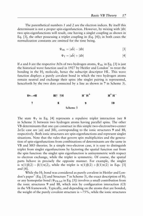
The parenthetical numbers 1 and 2 are the electron indices. By itself thisdeterminant is not a proper spin-eigenfunction. However, by mixing with jabjtwo spin-eigenfunctions will result, one having a singlet coupling as shown inEq. [3], the other possessing a triplet coupling in (Eq. [4]); in both cases thenormalization constants are omitted for the time being.

�HL ¼ jabj jabj ½3�

�T ¼ jabj þ jabj ½4�

If a and b are the respective AOs of two hydrogen atoms, �HL in Eq. [3] is justthe historical wave function used in 1927 by Heitler and London7 to treat thebonding in the H2 molecule, hence the subscript descriptor HL. This wavefunction displays a purely covalent bond in which the two hydrogen atomsremain neutral and exchange their spins (the singlet pairing is represented,henceforth by the two dots connected by a line as shown in 7 in Scheme 3).

The state �T in Eq. [4] represents a repulsive triplet interaction (see 8in Scheme 3) between two hydrogen atoms having parallel spins. The otherVB determinants that one can construct in this simple two-electron/two-center2e/2c case are jaaj and jbbj, corresponding to the ionic structures 9 and 10,respectively. Both ionic structures are spin-eigenfunctions and represent singletsituations. Note that the rules that govern spin multiplicities and the genera-tion of spin-eigenfunctions from combinations of determinants are the same inVB and MO theories. In a simple two-electron case, it is easy to distinguishtriplet from singlet eigenfunctions by factoring the spatial function out fromthe spin function: the singlet spin eigenfunction is antisymmetric with respectto electron exchange, while the triplet is symmetric. Of course, the spatialparts behave in precisely the opposite manner. For example, the singletis að1Þbð2Þ bð1Það2Þ, while the triplet is að1Þbð2Þ þ bð1Það2Þ in Eqs. [3]and [4].

While the H2 bond was considered as purely covalent in Heitler and Lon-don’s paper7 (Eq. [3] and Structure 7 in Scheme 3), the exact description of H2

or any homopolar bond (�VB-full in Eq. [5]) involves a small contribution fromthe ionic structures 9 and 10, which mix by configuration interaction (CI)in the VB framework. Typically, and depending on the atoms that are bonded,the weight of the purely covalent structure is �75%, while the ionic structures

Scheme 3

Basic VB Theory 17

share the remaining 25%. By symmetry, the wave function maintains an aver-age neutrality of the two bonded atoms (Eq. [5]).

�VB-full ¼ lðjabj jabjÞ þ mðjaaj þ jbbjÞ l > m ½5a�HaHb � 75%ðHa��HbÞ þ 25%ðHa Hþa þHþb Hb Þ ½5b�

For convenience, and to avoid confusion, we shall symbolize a purely covalentbond between A and B centers as A��B, while the notation AB will beemployed for a composite bond wave function like the one displayed in Eq.[5b]. In other words, AB refers to the ‘‘real’’ bond while A��B designatesits covalent component (see 2 in Scheme 1).

VB Wave Functions with Semilocalized AOsOne inconvenience of using the expression �VB-full (Eq. [5]) is its relative

complexity compared to the simpler HL function (Eq. [3]). Coulson andFischer111 proposed an elegant way of combining the simplicity of �HL

with the accuracy of �VB-full. In the Coulson–Fischer (CF) wave function,�CF, the two-electron bond is described as a formally covalent singlet couplingbetween two orbitals ja and jb, which are optimized with freedom to deloca-lize over the two centers. This is exemplified below for H2 (dropping onceagain the normalization factors):

�CF ¼ jjajbj jjajbj ½6a�ja ¼ aþ eb ½6b�jb ¼ bþ ea ½6c�

Here a and b are purely localized AOs, while ja and jb are delocalized AOs.In fact, experience shows that the Coulson–Fischer orbitals ja and jb, whichresult from the energy minimization, are generally not very delocalized (e < 1).As such they can be viewed as ‘‘distorted’’ orbitals that remain atomic-like innature. However minor this may look, the slight delocalization renders theCoulson–Fischer wave function equivalent to the VB-full (Eq. [5]) wave func-tion with the three classical structures. A straightforward expansion of theCoulson–Fischer wave function leads to a linear combination of classicalstructures in Eq. [7].

�CF ¼ ð1þ e2Þðjabj jabjÞ þ 2eðjaaj þ jbbjÞ ½7�

Thus, the Coulson–Fischer representation keeps the simplicity of the covalentpicture while treating the covalent–ionic balance by embedding the effect of theionic terms in a variational way through the delocalization tails. The Coulson–Fischer idea was later generalized to polyatomic molecules and gave rise to the


generalized valence bond (GVB) and spin-coupled (SC) methods, which werementioned in the introductory part and will be discussed later.

VB Wave Functions with Fragment OrbitalsValence bond determinants may involve fragment orbitals (FOs) instead

of localized or semilocalized AOs. These fragment orbitals may be delocalized(e.g., like some MOs of the constituent fragments of a molecule). The latteroption is an economical way of representing a wave function that is a linearcombination of several determinants based on AOs, just as MO determinantsare linear combinations of VB determinants (see below). Suppose, for exam-ple, that one wanted to treat the recombination of the CH�3 and H� radicalsin a VB manner. First, let (j1 j5) be the MOs of the CH�3 fragment (j5 beingsingly occupied), and b the AO of the incoming hydrogen. The covalent VBfunction that describes the active CH bond in our study just couples thej5 and b orbitals in a singlet way, as expressed in Eq. [8]:

�ðH3C��HÞ ¼ jj1j1j2j2j3j3j4j4 j5b j j1j1j2j2 j3 j3j4j4 j5bj j ½8�

Here, j1 j4 are fully delocalized on the CH3 fragment. Even the j5 orbital isnot a pure AO, but may involve some tails on the hydrogens of the fragment. Itis clear that this option is conceptually simpler than treating all the CHbonds in a VB way, including the ones that remain unchanged in the reaction.

Writing VB Wave Functions Beyond the 2e/2c CaseRules for writing VB wave functions in the polyelectronic case are just

intuitive extensions of the rules for the 2e/2c case discussed above. First, let

us consider butadiene, structure 11 in Scheme 4, and restrict the descriptionto the p system.

Denoting the p AOs of the C1–C4 carbons by a, b, c, and d, respectively,the fully covalent VB wave function for the p system of butadiene displays twosinglet couplings: one between a and b, and one between c and d. It followsthat the wave function can be expressed in the form of Eq. [9], as a product ofthe bond wave functions.

�ð11Þ ¼ jðab abÞ ðcd cdÞj ½9�

Scheme 4

Basic VB Theory 19

Upon expansion of the product, one gets a sum of four determinants as inEq. [10].

�ð11Þ ¼ jabcdj jabcdj jabcdj þ jabcdj ½10�

The product of bond wave functions in Eq. [9], involves so-called perfect pair-ing, whereby we take the Lewis structure of the molecule, represent each bondby a HL bond, and finally express the full wave function as a product of allthese pair-bond wave functions. As a rule, such a perfect-pairing polyelectro-nic VB wave function having n bond pairs will be described by 2n determi-nants, displaying all the possible 2� 2 spin permutations between theorbitals that are singlet coupled.

The above rule can readily be extended to larger polyelectronic systems,like the p system of benzene 12, or to molecules bearing lone pairs like forma-mide, 13. In this latter case, using n, c, and o, respectively, to refer to the pAOs of nitrogen, carbon, and oxygen, the VB wave function describing theneutral covalent structure is given by Eq. [11]:

�ð13Þ ¼ jnncoj jnn coj ½11�

In any one of the above cases, improvement of the wave function can beachieved by using Coulson–Fischer orbitals that take into account ionic con-tributions to the bonds. Note that the number of determinants grows exponen-tially with the number of covalent bonds (recall, this number is 2n, n being thenumber of bonds). Hence, 8 determinants are required to describe a Kekulestructure of benzene, and the fully covalent and perfectly paired wave functionfor methane is made of 16 determinants. This shows the benefit of using FOsrather than pure AOs as much as possible, as has been done above (Eq. [8]).Using FOs to construct VB wave functions is also appropriate when one wantsto fully exploit the symmetry properties of the molecule. For example, we candescribe all the bonds in methane by constructing group orbitals of the fourHs. Subsequently, we can distribute the eight bonding electrons of the mole-cule into these FOs as well as into the 2s and 2p AOs of carbon. Then we canpair up the electrons using orbital symmetry-matched FOs, as shown by thelines connecting these orbital pairs in Figure 1. The corresponding wave func-tion can be written as follows:

�ðCH4Þ ¼ jð2sjs js2sÞð2pxjx jx2pxÞð2pyjy jy 2pyÞð2pzjz jz 2pzÞj½12�

In this representation, each bond is a delocalized covalent two-electron bond,written as a HL-type bond. The VB method that deals with fragment orbitals


(FO–VB) is particularly useful in high-symmetry cases such as ferrocene andother organometallic complexes.

Pictorial Representation of VB Wave Functions by Bond DiagramsSince we argue that a bond need not necessarily involve only two AOs on

two centers, we must provide an appropriate pictorial representation of such abond. A possibility is the bond diagram in Figure 2, which shows two spin-paired electrons in general orbitals j1 and j2, with a line connecting theseorbitals. This bond diagram represents the wave function in Eq. [13]

�bond ¼ jj1j2j jj1j2j ½13�

where the orbitals can take any shape; it can involve two centers with localizedAOs, or two Coulson–Fischer orbitals with delocalization tails, or FOs thatspan multiple centers.

Figure 1 A VB representation of methane using delocalized FOs. Each line that connectsthe orbitals is a bond pair. The total wave function is given in Eq. 12.

Figure 2 A bond diagram representation of two spin-paired electrons in orbitals f1 andf2. The bond pair is indicated by a line connecting the orbitals.

Basic VB Theory 21

The Relationship between MO and VB Wave Functions

We now consider the difference between the MO and VB descriptions ofan electronic system, at the simplest level of both theories. As we shall see, inthe cases of one-electron, three-electron, and four-electron interactionsbetween two centers, there is no real difference between the two theories,except for a matter of language. However, the two theories do differ in theirdescription of the two-electron bond. Let us consider, once again, the exampleof H2, with its two AOs a and b, and examine first the VB description, drop-ping normalization factors for simplicity.

As has been stated already, at equilibrium distance the bonding is not100% covalent, and requires an ionic component to be accurately described.On the other hand, at long distances the HL wave function is the correct state,as the ionic components necessarily drop to zero and each hydrogen carriesone electron away through the homolytic bond breaking. The HL wave func-tion dissociates correctly, but is quantitatively inaccurate at bonding distances.Therefore, the way to improve the HL description is straightforward: simplymixing �HL with the ionic determinants and optimizing the coefficients varia-tionally, by CI. One then gets the wave function �VB-full, in Eq. [5a] above,which contains a major covalent component and a minor ionic one.

Let us now turn to the MO description. Bringing together two hydrogenatoms leads to the formation of two MOs, s and s� (bonding and antibond-ing, respectively); see Eq. [14].

s ¼ aþ b s� ¼ a b ½14�

At the simple MO level, the ground state of H2 is described by �MO, in whichthe bonding s MO is doubly occupied. Expansion (see Appendix for details)of this MO determinant into its AO determinant constituents leads to Eq. [15]:

�MO ¼ jssj ¼ ðjabj jabjÞ þ ðjaaj þ jbbjÞ ½15�

It is apparent from Eq. [15] that the first half of the expansion is just theHeitler–London function �HL (Eq. [3]), while the remaining part is ionic. Itfollows that the MO description of the two-electron bond will always behalf-covalent, half-ionic, irrespective of the bonding distance. Qualitatively,it is already clear that in the MO wave function, the ionic weight is excessiveat bonding distances, and becomes an absurdity at long distances, where theweight of the ionic structures should drop to zero in accord with homolyticcleavage. The simple MO description does not dissociate correctly and thisis the reason why it is inappropriate for the description of stretched bondsas, for example, those found in transition states. The remedy for this poordescription is CI, specifically the mixing of the ground configuration, s2,with the diexcited one, s�2. The reason this mixing resizes the covalent versus


ionic weights is the following: If one expands the diexcited configuration, �D,into its VB constituents (for expansion technique, see Appendix A.1), one findsthe same covalent and ionic components as in Eq. [15], but coupled with anegative sign as in Eq. [16]:

�D ¼ js�s�j ¼ ðjabj jabjÞ þ ðjaaj þ jbbjÞ ½16�

It follows that mixing the two configurations �MO and �D with differentcoefficients as in Eq. [17] will lead to a wave function �MO–CI in which thecovalent and ionic components have

�MO--CI ¼ c1jssj c2js�s�j c1; c2 > 0 ½17�

unequal weights, as shown by an expansion of �MO–CI into AO determinantsin Eq. [18]:

�MO--CI ¼ ðc1 þ c2Þðjabj jabjÞ þ ðc1 c2Þðjaaj þ jbbjÞ ½18a�c1 þ c2 ¼ l c1 c2 ¼ m ½18b�

Since c1 and c2 are variationally optimized, expansion of �MO–CI should leadto exactly the same VB function as �VB–full in Eq. [5], leading to the equalitiesexpressed in Eq. [18b] and to the equivalence of �MO–CI and �VB–full. Theequivalence also includes the Coulson–Fischer wave function �CF (Eq. [6])which, as we have seen, is equivalent to the VB-full description.

�MO 6¼ �HL �MO--CI � �VB--full � �CF ½19�

To summarize, the simple MO treatment describes the bond as being tooionic, while the simple VB level (Heitler–London) defines it as being purelycovalent. Both theories converge to the right description when CI is intro-duced. The accurate description of two-electron bonding is half-way betweenthe simple MO and simple VB levels; elaborated MO and VB levels becomeequivalent and converge to the right description, in which the bond is mostlycovalent but has a substantial contribution from ionic structures.

This equivalence clearly indicates that the MO–VB rivalry, discussedabove, is unfortunate and senseless. VB and MO are not two diametrically dif-ferent theories that exclude each other, but rather two representations of rea-lity that are mathematically equivalent. The best approach is to use these tworepresentations jointly and benefit from their complementary insight. In fact,from the above discussion of how to write a VB wave function, it is apparentthat there is a spectrum of orbital representations that stretches between thefully local VB representations through semilocalized CF orbitals, to theuse of delocalized fragment orbitals VB (FO–VB), and all the way to the fully

Basic VB Theory 23

delocalized MO representation (in the MO–CI language). Based on the pro-blem at hand, the best representation from this spectrum should be the onethat gives the clearest and most portable insight into the problem.

Formalism Using the Exact Hamiltonian

Let us turn now to the calculation of energetic quantities using exact VBtheory by considering the simple case of the H2 molecule. The exact Hamilto-nian is of course the same as in MO theory, and is composed in this case of twocore terms and a bielectronic repulsion:

H ¼ hð1Þ þ hð2Þ þ 1=r12 þ 1=R ½20�

where the h operator represents the attraction between one electron and thenuclei, r12 is the interelectronic distance and R is the distance between thenuclei and accounts for nuclear repulsion. In the VB framework, some parti-cular notations are traditionally employed to designate the various energiesand matrix elements:

Q ¼ hjabjjHjjabji ¼ hajhjai þ hbjhjbi þ habj1=r12jabi ½21�K ¼ hjabjjHjjbaji ¼ habj1=r12jabi þ 2Shajhjbi ½22�hðjabjÞjðjbajÞi ¼ S2 ½23�

Here Q is the energy of a single determinant jabj, K is the spin exchangeterm which will be dealt with later, and S is the overlap integral between thetwo AOs a and b.

The energy Q has an interesting property: It is quasiconstant as a functionof the interatomic distance, from infinite distance to the equilibrium bondingdistance Req of H2. It corresponds to the energy of two hydrogen atoms whenbrought together without exchanging their spins. Such a pseudo-state (which isnot a spin-eigenfunction) is called the ‘‘quasi-classical state’’ of H2 (�QC inFig. 3), because all the terms of its energy have an analogue in classical (notquantum) physics. Turning now to real states, that is, spin-eigenfunctions, theenergy of the ground state of H2, in the fully covalent approximation of HL, isreadily obtained.

Eð�HLÞ ¼hðj ab j ja b jÞjH jðj ab j j ab jÞ ihðj ab j j ab jÞjðj ab j j abjÞi

¼ Qþ K

1þ S2½24�

Plotting the E(�HL) curve as a function of the distance now gives qualitativelycorrect Morse curve behavior (Fig. 3), with a reasonable bonding energy, evenif a deeper potential well can be obtained by allowing further mixing with the


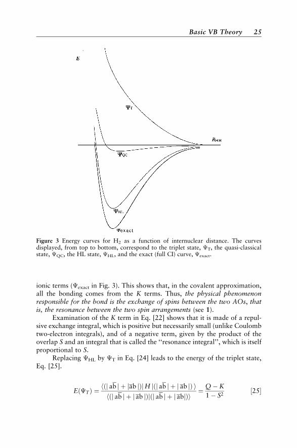
ionic terms (�exact in Fig. 3). This shows that, in the covalent approximation,all the bonding comes from the K terms. Thus, the physical phenomenonresponsible for the bond is the exchange of spins between the two AOs, thatis, the resonance between the two spin arrangements (see 1).

Examination of the K term in Eq. [22] shows that it is made of a repul-sive exchange integral, which is positive but necessarily small (unlike Coulombtwo-electron integrals), and of a negative term, given by the product of theoverlap S and an integral that is called the ‘‘resonance integral’’, which is itselfproportional to S.

Replacing �HL by �T in Eq. [24] leads to the energy of the triplet state,Eq. [25].

Eð�TÞ ¼hðj ab j þ jab jÞjH jðj ab j þ j ab jÞ ihðj ab j þ j ab jÞjðj ab j þ j abjÞi

¼ Q K

1 S2½25�

Figure 3 Energy curves for H2 as a function of internuclear distance. The curvesdisplayed, from top to bottom, correspond to the triplet state, �T, the quasi-classicalstate, �QC, the HL state, �HL, and the exact (full CI) curve, �exact.

Basic VB Theory 25

Recalling that the Q integral is a quasi-constant from Req to infinite distance,Q remains nearly equal to the energy of the separated fragments and can serve,at any distance, as a reference for the bond energy. It follows from Eqs. [24]and [25] that, if we neglect overlap in the denominator, the triplet state (�T inFig. 3) is repulsive by the same quantity (K) as the singlet is bonding (þK).Thus, at any distance larger than Req, the bonding energy is about one-half ofthe singlet–triplet gap. This property will be used later in applications to reac-tivity.

Qualitative VB Theory

A VB calculation is just a configuration interaction in a space of AO orFO determinants, which are in general nonorthogonal to each other. It istherefore essential to derive some basic rules for calculating the overlapsand Hamiltonian matrix elements between determinants. The fully generalrules have been described in detail elsewhere.52 Examples will be given herefor commonly encountered simple cases.

Overlaps between DeterminantsLet us illustrate the procedure with VB determinants of the type � and �0

below,

� ¼ Njaabbj �0 ¼ N0jccddj ½26�

where N and N0 are normalization factors. Each determinant is made of adiagonal product of spin orbitals followed by a signed sum of all the permuta-tions of this product, which are obtained by transposing the order of the spinorbitals. Denoting the diagonal products of � and �0, by �d and �0d, respec-tively, the expression for �d reads

�d ¼ að1Þ að2Þ bð3Þ bð4Þ ð1;2; . . . are electron indicesÞ ½27�

and an analogous expression can be written for �0d.The overlap between the (unnormalized) determinants j a a b b j and

j c c d d j is given by Eq. [28]:

hðj a a b b j Þðj c c d d j Þi ¼ �d

��XP

ð1ÞtPð�0dÞ* +

½28�

where the operator P represents a restricted subset of permutations: The onesmade of pairwise transpositions between spin orbitals of the same spin, and tdetermines the parity, odd or even, and hence also the sign of a given pairwise


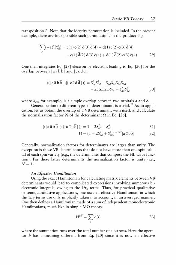
transposition P. Note that the identity permutation is included. In the presentexample, there are four possible such permutations in the product �0d:

XP

ð1ÞtPð0dÞ ¼ cð1Þ cð2Þ dð3Þ dð4Þ dð1Þ cð2Þ cð3Þ dð4Þ

cð1Þ dð2Þ dð3Þ cð4Þ þ dð1Þ dð2Þ cð3Þ cð4Þ ½29�

One then integrates Eq. [28] electron by electron, leading to Eq. [30] for theoverlap between j a a b b j and j c c d d j:

hðj a a b b j Þjðj c c d d j Þi ¼ S2acS

2bd SadSacSbcSbd

SacSadSbdSbc þ S2adS2

bc ½30�

where Sac, for example, is a simple overlap between two orbitals a and c.Generalization to different types of determinants is trivial.52 As an appli-

cation, let us obtain the overlap of a VB determinant with itself, and calculatethe normalization factor N of the determinant � in Eq. [26]:

hðj a a b b j Þjðj a a b b j Þi ¼ 1 2S2ab þ S4

ab ½31�� ¼ ð1 2S2

ab þ S4abÞ 1=2ja a bbj ½32�

Generally, normalization factors for determinants are larger than unity. Theexception is those VB determinants that do not have more than one spin orbi-tal of each spin variety (e.g., the determinants that compose the HL wave func-tion). For these latter determinants the normalization factor is unity (i.e.,N ¼ 1).

An Effective HamiltonianUsing the exact Hamiltonian for calculating matrix elements between VB

determinants would lead to complicated expressions involving numerous bi-electronic integrals, owing to the 1/rij terms. Thus, for practical qualitativeor semiquantitative applications, one uses an effective Hamiltonian in whichthe 1/rij terms are only implicitly taken into account, in an averaged manner.One then defines a Hamiltonian made of a sum of independent monoelectronicHamiltonians, much like in simple MO theory:

Heff ¼X

i

hðiÞ ½33�

where the summation runs over the total number of electrons. Here the opera-tor h has a meaning different from Eq. [20] since it is now an effective

Basic VB Theory 27

monoelectronic operator that incorporates part of the electron–electron andnuclear–nuclear repulsions. Going back to the four–electron example above,the determinants � and �0 are coupled by the following effective Hamiltonianmatrix element:

h�jHeffj�0i ¼ h�jhð1Þ þ hð2Þ þ hð3Þ þ hð4Þj�0i ½34�

It is apparent that the above matrix element is composed of a sum of fourterms that are calculated independently. The calculation of each of these terms(e.g., the first one) is quite analogous to the calculation of the overlap in Eq.[30], except that the first monoelectronic overlap S in each product is replacedby a monoelectronic Hamiltonian term:

hðj a a b b jÞj hð1Þ jðj c c d d jÞ i ¼ hacSacS2bd hadSacSbcSbd

hacSadSbdSbc þ hadSadS2bc ½35a�

hac ¼ hajhjci ½35b�

In Eq. [35b], the monoelectronic integral accounts for the interaction betweentwo overlapping orbitals. A diagonal term of the type haa is interpreted as theenergy of the orbital a, and will be noted ea in the following equations. Byusing Eqs. [34] and [35], it is easy to calculate the energy of the determinantj a a bb j:

EðjaabbjÞ ¼ N2ð2ea þ 2eb 2eaS2ab 2ebS2

ab 4habSab þ 4habS3abÞ ½36�

An interesting application of the above rules is the calculation of theenergy of a spin-alternant determinant such as 14 in Scheme 5 for butadiene.

Such a determinant, in which the spins are arranged so that two neigh-boring orbitals always display opposite spins is referred to as a ‘‘quasiclassi-cal’’ (QC) state and is a generalization of the QC state that we alreadyencountered above for H2. The rigorous formulation of its energy involvessome terms that arise from permutations between orbitals of the same spins,which are necessarily nonneighbors. Neglecting interactions between non-nearest neighbors, all these vanish, so that the energy of the QC state is givenby the simple expression below.

Ej a b c d j ¼ ea þ eb þ ec þ ed ½37�

Scheme 5


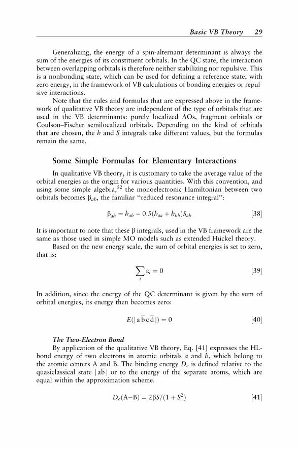
Generalizing, the energy of a spin-alternant determinant is always thesum of the energies of its constituent orbitals. In the QC state, the interactionbetween overlapping orbitals is therefore neither stabilizing nor repulsive. Thisis a nonbonding state, which can be used for defining a reference state, withzero energy, in the framework of VB calculations of bonding energies or repul-sive interactions.

Note that the rules and formulas that are expressed above in the frame-work of qualitative VB theory are independent of the type of orbitals that areused in the VB determinants: purely localized AOs, fragment orbitals orCoulson–Fischer semilocalized orbitals. Depending on the kind of orbitalsthat are chosen, the h and S integrals take different values, but the formulasremain the same.

Some Simple Formulas for Elementary Interactions

In qualitative VB theory, it is customary to take the average value of theorbital energies as the origin for various quantities. With this convention, andusing some simple algebra,52 the monoelectronic Hamiltonian between twoorbitals becomes bab, the familiar ‘‘reduced resonance integral’’:

bab ¼ hab 0:5ðhaa þ hbbÞSab ½38�

It is important to note that these b integrals, used in the VB framework are thesame as those used in simple MO models such as extended Huckel theory.

Based on the new energy scale, the sum of orbital energies is set to zero,that is: X

i

ei ¼ 0 ½39�

In addition, since the energy of the QC determinant is given by the sum oforbital energies, its energy then becomes zero:

Eðj a b c d jÞ ¼ 0 ½40�

The Two-Electron BondBy application of the qualitative VB theory, Eq. [41] expresses the HL-

bond energy of two electrons in atomic orbitals a and b, which belong tothe atomic centers A and B. The binding energy De is defined relative to thequasiclassical state j ab j or to the energy of the separate atoms, which areequal within the approximation scheme.

DeðABÞ ¼ 2bS=ð1þ S2Þ ½41�

Basic VB Theory 29

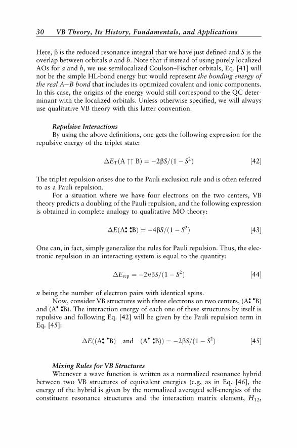
Here, b is the reduced resonance integral that we have just defined and S is theoverlap between orbitals a and b. Note that if instead of using purely localizedAOs for a and b, we use semilocalized Coulson–Fischer orbitals, Eq. [41] willnot be the simple HL-bond energy but would represent the bonding energy ofthe real AB bond that includes its optimized covalent and ionic components.In this case, the origins of the energy would still correspond to the QC deter-minant with the localized orbitals. Unless otherwise specified, we will alwaysuse qualitative VB theory with this latter convention.

Repulsive InteractionsBy using the above definitions, one gets the following expression for the

repulsive energy of the triplet state:

�ETðA "" BÞ ¼ 2bS=ð1 S2Þ ½42�

The triplet repulsion arises due to the Pauli exclusion rule and is often referredto as a Pauli repulsion.

For a situation where we have four electrons on the two centers, VBtheory predicts a doubling of the Pauli repulsion, and the following expressionis obtained in complete analogy to qualitative MO theory:

�EðA�� BÞ ¼ 4bS=ð1 S2Þ ½43�

One can, in fact, simply generalize the rules for Pauli repulsion. Thus, the elec-tronic repulsion in an interacting system is equal to the quantity:

�Erep ¼ 2nbS=ð1 S2Þ ½44�

n being the number of electron pairs with identical spins.Now, consider VB structures with three electrons on two centers, (A�� B)

and (A� ��B). The interaction energy of each one of these structures by itself isrepulsive and following Eq. [42] will be given by the Pauli repulsion term inEq. [45]:

�EððA�� BÞ and ðA� ��BÞÞ ¼ 2bS=ð1 S2Þ ½45�

Mixing Rules for VB StructuresWhenever a wave function is written as a normalized resonance hybrid

between two VB structures of equivalent energies (e.g, as in Eq. [46], theenergy of the hybrid is given by the normalized averaged self-energies of theconstituent resonance structures and the interaction matrix element, H12,


between the structures in Eq. [47].

� ¼ N½�1 þ �2�where N ¼ 1=½2ð1þ S12Þ�1=2 ½46�

Eð�Þ ¼ 2N2Eav þ 2N2H12

where H12 ¼ h�1jHj�2i and Eav ¼ ½ðE1 þ E2Þ=2� ½47�

Such a mixed state is stabilized relative to the energy of each individual VBstructure, by a quantity that is called the ‘‘resonance energy’’ (RE):

RE ¼ ½H12 EavS12�=ð1þ S12Þ S12 ¼ h�1j�2i ½48�

Equation [48] expresses the RE in the case where the two limiting structures�1 and �2 have equal or nearly equal energies, which is the most favorablesituation for maximum stabilization. However, if the energies E1 and E2 aredifferent, then according to the rules of perturbation theory, the stabilizationwill still be significant, albeit than in the degenerate case.

A typical situation where the VB wave function is written as a resonancehybrid is odd-electron bonding (one-electron or three-electron bonds). Forexample, a one-electron bond A�B is a situation where only one electron isshared by two centers A and B (Eq. [49]), while three electrons are distributedover the two centers in a three-electron bond A;B (Eq. [50]):

A�B ¼ Aþ�B$ A� þB ½49�

A;B ¼ A� ��B$ A��

�B ½50�

Simple algebra shows that the overlap between the two VB structures is equalto S (the hajbi orbital overlap)a and that resonance energy follows Eq. [51]:

RE ¼ b=ð1þ SÞ ¼ DeðAþ �B$ A� þBÞ ½51�

Equation [51] also gives the bonding energy of a one-electron bond. Combin-ing Eqs. [45] and [51], we get the bonding energy of the three-electron bond,Eq. [52]:

DeðA� ��B$ A��BÞ ¼ 2bS=ð1 S2Þ þ b=ð1þ SÞ¼ bð1 3SÞ=ð1 S2Þ ½52�

a Writing f1 and f2 so that their positive combination is the resonance-stabilized one.

Basic VB Theory 31

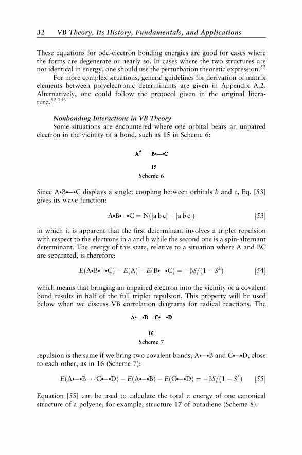
These equations for odd-electron bonding energies are good for cases wherethe forms are degenerate or nearly so. In cases where the two structures arenot identical in energy, one should use the perturbation theoretic expression.52

For more complex situations, general guidelines for derivation of matrixelements between polyelectronic determinants are given in Appendix A.2.Alternatively, one could follow the protocol given in the original litera-ture.52,143

Nonbonding Interactions in VB TheorySome situations are encountered where one orbital bears an unpaired

electron in the vicinity of a bond, such as 15 in Scheme 6:

Since A�B��C displays a singlet coupling between orbitals b and c, Eq. [53]gives its wave function:

A�B��C ¼ Nðja b cj ja b cjÞ ½53�

in which it is apparent that the first determinant involves a triplet repulsionwith respect to the electrons in a and b while the second one is a spin-alternantdeterminant. The energy of this state, relative to a situation where A and BCare separated, is therefore:

EðA�B��CÞ EðAÞ EðB��CÞ ¼ bS=ð1 S2Þ ½54�

which means that bringing an unpaired electron into the vicinity of a covalentbond results in half of the full triplet repulsion. This property will be usedbelow when we discuss VB correlation diagrams for radical reactions. The

repulsion is the same if we bring two covalent bonds, A��B and C��D, closeto each other, as in 16 (Scheme 7):

EðA��B � � �C��DÞ EðA��BÞ EðC��DÞ ¼ bS=ð1 S2Þ ½55�

Equation [55] can be used to calculate the total p energy of one canonicalstructure of a polyene, for example, structure 17 of butadiene (Scheme 8).

Scheme 6

Scheme 7


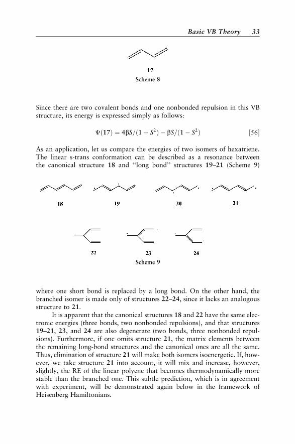
Since there are two covalent bonds and one nonbonded repulsion in this VBstructure, its energy is expressed simply as follows:

�ð17Þ ¼ 4bS=ð1þ S2Þ bS=ð1 S2Þ ½56�

As an application, let us compare the energies of two isomers of hexatriene.The linear s-trans conformation can be described as a resonance betweenthe canonical structure 18 and ‘‘long bond’’ structures 19–21 (Scheme 9)

where one short bond is replaced by a long bond. On the other hand, thebranched isomer is made only of structures 22–24, since it lacks an analogousstructure to 21.

It is apparent that the canonical structures 18 and 22 have the same elec-tronic energies (three bonds, two nonbonded repulsions), and that structures19–21, 23, and 24 are also degenerate (two bonds, three nonbonded repul-sions). Furthermore, if one omits structure 21, the matrix elements betweenthe remaining long-bond structures and the canonical ones are all the same.Thus, elimination of structure 21 will make both isomers isoenergetic. If, how-ever, we take structure 21 into account, it will mix and increase, however,slightly, the RE of the linear polyene that becomes thermodynamically morestable than the branched one. This subtle prediction, which is in agreementwith experiment, will be demonstrated again below in the framework ofHeisenberg Hamiltonians.

Scheme 8

Scheme 9

Basic VB Theory 33

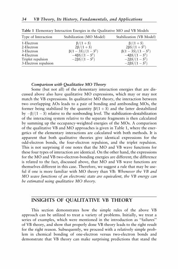
Comparison with Qualitative MO TheorySome (but not all) of the elementary interaction energies that are dis-

cussed above also have qualitative MO expressions, which may or may notmatch the VB expressions. In qualitative MO theory, the interaction betweentwo overlapping AOs leads to a pair of bonding and antibonding MOs, theformer being stabilized by the quantity b/(1þ S) and the latter destabilizedby b=ð1 S) relative to the nonbonding level. The stabilization–destabilizationof the interacting system relative to the separate fragments is then calculatedby summing up the occupancy-weighted energies of the MOs. A comparisonof the qualitative VB and MO approaches is given in Table 1, where the ener-getics of the elementary interactions are calculated with both methods. It isapparent that both qualitative theories give identical expressions for theodd-electron bonds, the four-electron repulsion, and the triplet repulsion.This is not surprising if one notes that the MO and VB wave functions forthese four types of interaction are identical. On the other hand, the expressionsfor the MO and VB two-electron-bonding energies are different; the differenceis related to the fact, discussed above, that MO and VB wave functions arethemselves different in this case. Therefore, we suggest a rule that may be use-ful if one is more familiar with MO theory than VB: Whenever the VB andMO wave functions of an electronic state are equivalent, the VB energy canbe estimated using qualitative MO theory.

INSIGHTS OF QUALITATIVE VB THEORY

This section demonstrates how the simple rules of the above VBapproach can be utilized to treat a variety of problems. Initially, we treat aseries of examples, which were mentioned in the introduction as ‘‘failures’’of VB theory, and show that properly done VB theory leads to the right resultfor the right reason. Subsequently, we proceed with a relatively simple prob-lem in chemical bonding of one-electron versus two-electron bonds anddemonstrate that VB theory can make surprising predictions that stand the

Table 1 Elementary Interaction Energies in the Qualitative MO and VB Models

Type of Interaction Stabilization (MO Model) Stabilization (VB Model)

1-Electron b=ð1þ SÞ b=ð1þ SÞ2-Electron 2b=ð1þ SÞ 2bS=ð1þ S2Þ3-Electron bð1 3SÞ=ð1 S2Þ bð1 3SÞ=ð1 S2Þ4-Electron 4bS=ð1 S2Þ 4bS=ð1 S2ÞTriplet repulsion 2bS=ð1 S2Þ 2bS=ð1 S2Þ3-Electron repulsion 2bS=ð1 S2Þ


test of experiment. Finally, we show how VB theory can lead to a generalmodel for chemical reactivity, the VB diagram. Since these subtopics cover awide range of chemical problems we cannot obviously treat them in-depth,and wherever possible we refer the reader to more extensive reviews.

Are the ‘‘Failures’’ of VB Theory Real?

As mentioned in the introduction, VB theory has been accused of a few‘‘failures’’ that are occasionally used to dismiss the theory, and have caused itto have an unwarranted reputation. The next few subsections use the simpleVB guidelines drawn above to demonstrate that VB theory is free of these‘‘failures’’.

DioxygenOne of the major ‘‘failures’’ that has been associated with VB theory con-

cerns the ground state of the dioxygen molecule, O2. It is true that a naiveapplication of hybridization followed by perfect pairing (simple Lewis pairing)would predict a 1�g ground state, that is, the diamagnetic doubly bondedmolecule OO. This is likely the origin of the notion that VB theory makesa flawed prediction that contradicts experiment (see, e.g., references [50] and[51]). However, this conclusion is not valid, since in the early 1970s Goddardet al.107 performed GVB calculations and demonstrated that VB theory pre-dicts a triplet 3�g ground state. This same outcome was reported in papersby McWeeny144 and Harcourt.145 In fact, any VB calculation, at whateverimagined level, would lead to the same result, so the myth of ‘‘failure’’ is defi-nitely baseless.

Goddard et al.107 and subsequently the present two authors53 also pro-vided a simple VB explanation for the choice of the ground state. Let us reiter-ate this explanation based on our qualitative VB theory, outlined above.

Apart from one s bond and one s lone pair on each oxygen atom, thedioxygen molecule has six p electrons to be distributed in the two p planes, saypx and py. The question is What is the most favorable mode of distribution? Isit 25 in which three electrons are placed in each p plane, or perhaps is it 26where two electrons are allocated to one plane and four to the other (Scheme10)? Obviously, 25 is a diradical structure displaying one three-electron bond

Scheme 10

Insights of Qualitative VB Theory 35

in each of p planes, whereas 26 exhibits a singlet p bond, in one plane, and afour-electron repulsion, in the other. A naive application that neglects therepulsive three-electron and four-electron interactions would predict thatstructure 26 is preferred, leading to the above-mentioned legendary failureof VB theory, namely, that VB predicts the ground state of O2 to be the singletclosed-shell structure, OO. Inspection of the repulsive interactions showsthat they are of the same order of magnitude or even larger than the bondinginteractions, that is, the neglect of these repulsion is unjustified. The rightanswer is immediately apparent, if we carry out the VB calculation correctly,including the repulsion and bonding interactions for structures 25 and 26. Theresulting expressions and the respective energy difference, which are shown inEqs. [57–59], demonstrate clearly that the diradical structure 25 is more stablethan the doubly bonded Lewis structures 26.

Eð25Þ ¼ 2bð1 3SÞ=ð1 S2Þ ½57�Eð26Þ ¼ 2bS=ð1þ S2Þ 4bS=ð1 S2Þ ½58�

Eð26Þ Eð25Þ ¼ 2bð1 SÞ2=ð1 S4Þ > 0 ½59�

Thus far we have not considered the set of Slater determinants 250 and260, which are symmetry-equivalent to 25 and 26 by inversion of the px and py

planes. The interactions between the two sets of determinants yield two pairsof resonant–antiresonant combinations that constitute the final low-lying statesof dioxygen, as represented in Figure 4. Of course, our effective VB theorywas chosen to disregard the bielectronic terms and, therefore, the theory, as

Figure 4 Formation of the symmetry adapted states of O2 from the biradical (25, 250)and perfectly-paired (26, 26’) structures.


such, will not tell us what the lowest spin state in the O2 diradical is. This,however, is a simple matter, because further considerations can be made byappealing to Hund’s rule, which is precisely what qualitative MO theorymust do in order to predict the triplet nature of the O2 ground state. Accord-ingly, the in-phase and out-of-phase combinations of the diradical determi-nants 25 and 250 lead to triplet (3�g ) and singlet (1�g) states, respectively,the former being the lowest state by virtue of favorable exchange energy.

Similarly, 26 and 260 yield a resonant 1�g combination and an antireso-nant 1�þg one. Thus, it is seen that simple qualitative VB considerations notonly predict the ground state of O2 to be a triplet, but also yield a correctenergy ordering for the remaining low-lying excited states.

The Valence Ionization Spectrum of CH4

As discussed in the introduction, the development of PES showed thatthe spectra could be simply interpreted if one assumed that electrons occupydelocalized molecular orbitals.47,48 By contrast, VB theory, which uses loca-lized bond orbitals (LBOs), seems completely useless for interpretation ofPES. Moreover, since VB theory describes equivalent electron pairs that occupyLBOs, the PES results seem to be in disagreement with this theory. An iconicexample of this ‘‘failure’’ of VB theory is the PES of methane that displays twodifferent ionization peaks. These peaks correspond to the a1 and t2 MOs, butnot to the four equivalent CH LBOs in Pauling’s hybridization theory.

Let us now examine the problem carefully in terms of LBOs to demon-strate that VB gives the right result for the right reason. A physically correctrepresentation of the CHþ4 cation would be a linear combination of the fourforms such that the wave function does not distinguish the four LBOs thatare related by symmetry. The corresponding VB picture, more specifically anFO–VB picture, is illustrated in Figure 5, which enumerates the VB structuresand their respective determinants. Each VB structure involves a localized one-electron bond situation, while the other bonds are described by doubly occu-pied LBOs. To make life easier, we can use LBOs that derive from a unitarytransformation of the canonical MOs. As such, these LBOs would be orthogo-nal to each other and one can calculate the Hamiltonian matrix elementbetween two such VB structures by simply setting all overlaps to zero in theVB expressions, or by using the equivalent rules of qualitative MO theory.Thus, to calculate the �1–�2 interaction matrix element, one first puts theorbitals of both determinants in maximal correspondence, by means of a trans-position in �2. The resulting two transformed determinants differ by only onespin orbital, c 6¼ d, so that their matrix element is simply b. Going back to theoriginal �1 and �2 determinants, it appears that their matrix element is nega-tively signed (Eq. [60]),

h�1jHeffj�2i ¼ hðj a a b b c c d jÞjHeff jðj d d a a b b c jÞi¼ hðj a a b b c c d jÞjHeff jðj a a b b c d d jÞi ¼ b ½60�


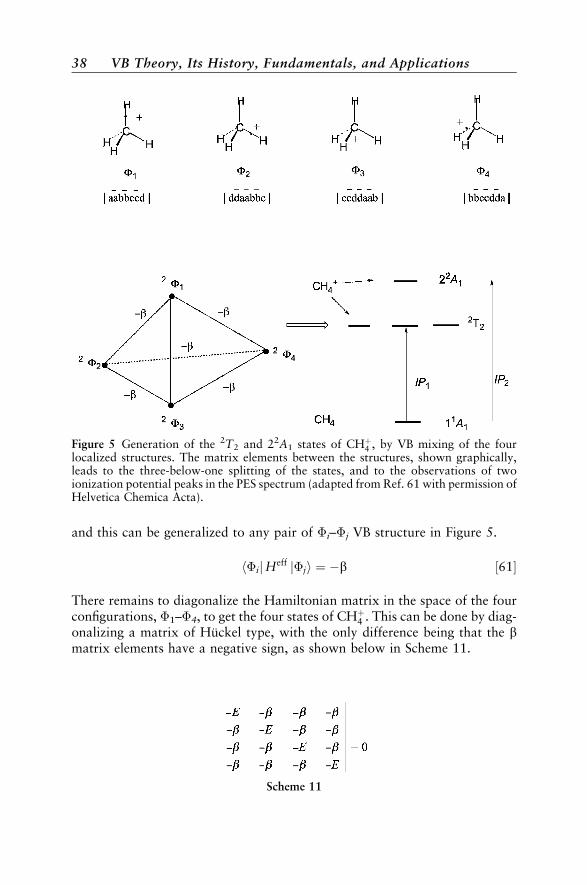
and this can be generalized to any pair of �i–�j VB structure in Figure 5.

h�ijHeff j�ji ¼ b ½61�

There remains to diagonalize the Hamiltonian matrix in the space of the fourconfigurations, �1–�4, to get the four states of CHþ4 . This can be done by diag-onalizing a matrix of Huckel type, with the only difference being that the bmatrix elements have a negative sign, as shown below in Scheme 11.

Figure 5 Generation of the 2T2 and 22A1 states of CHþ4 , by VB mixing of the fourlocalized structures. The matrix elements between the structures, shown graphically,leads to the three-below-one splitting of the states, and to the observations of twoionization potential peaks in the PES spectrum (adapted from Ref. 61 with permission ofHelvetica Chemica Acta).

Scheme 11


The diagonalization can be done using a Huckel program; however, theresult can be found even without any calculation (e.g, by use of symmetry pro-jection operators of the Td point group). Diagonalization of the above Huckelmatrix, with negatively signed b leads to the final states of CHþ4 , shown along-side the interaction graph in Figure 5. These cationic states exhibit a three-below-one splitting (i.e., a low-lying triply degenerate 2T2 state and above ita 2A1 state). The importance of the sign of the matrix element can be appre-ciated by diagonalizing the above Huckel matrix using a positively signed b.Doing that would have reversed the state ordering to one-below-three, whichis of course incorrect. Thus, simple VB theory correctly predicts that methanewill have two ionization peaks, one (IP1) at lower energy corresponding totransition to the degenerate 2T2 state and one (IP2) at a higher energy corre-sponding to transition to the 2A1 state. The facility of making this predictionand its agreement with experiment show once more that, here, too, the ‘‘fail-ure’’ of VB theory is due more to a myth that caught on due to the naivety ofthe initial argument than to any true failure of VB.

Aromaticity–AntiaromaticityAs discussed in the introduction, simple resonance theory completely

fails to predict the fundamental differences between C5Hþ5 and C5H5 ,C3Hþ3 , and C3H3 , C7Hþ7 , and C7H7 , and so on. Hence, a decisive defeatwas dealt to VB theory when, during the 1950–1960s, organic chemistswere finally able to synthesize these transient molecules and establish their sta-bility patterns (which followed Huckel rules) with no guide or insight comingfrom resonance theory. We shall now demonstrate (which has been known forquite a while52,146,147) that the simple VB theory outlined above is capable ofderiving the celebrated 4nþ 2=4n dichotomy for these ions.

As an example, we compare the singlet and triplet states of the cyclopro-penium molecular ions, C3Hþ3 and C3H3 , shown in Figures 6 and 7. The VBconfigurations needed to generate the singlet and triplet states of the equilat-eral triangle C3Hþ3 are shown in Figure 6. It is seen that the structures can begenerated from one another by shifting single electrons from a singly occupiedpp orbital to a vacant one. By using the guidelines for VB matrix elements (seeAppendix A.2), we deduce that the leading matrix element between any pair ofstructures with singlet spins is þb, while for any pair with triplet spin thematrix element is b. The corresponding configurations of C3H3 are shownin Figure 7. In this case, the signs of the matrix elements are inverted comparedwith the case of the cyclopropenium cation, and are b for any pair of singletVB structures, and þb for any pair of triplet structures.

If we symbolize the VB configurations by heavy dots we can present theseresonance interactions graphically, as shown in the mid-parts of Figures 6 and7. These interaction graphs are all triangles and have the topology of corre-sponding Huckel and Mobius AO interactions.148 Of course, one could diag-onalize the corresponding Huckel–Mobius matrices and obtain energy levels


and wave functions, but a shortcut based on the well-known mnemonic ofFrost and Musulin149 exists. A triangle is inscribed within a circle having aradius 2jbj, and the energy levels are obtained from the points where the ver-tices of the triangle touch the circle. Using this mnemonic for the VB mixingshows that the ground state of C3Hþ3 is a singlet state, while the triplet state ishigher lying and doubly degenerate. By contrast, the ground state of C3H3 is atriplet state, while the singlet state is higher lying, doubly degenerate, and

Figure 6 The VB structures for singlet and triplet states of C3Hþ3 , along with thegraphical representation of their interaction matrix elements (adapted from Ref. 61 withpermission of Helvetica Chemica Acta). The spread of the states is easily predicted fromthe circle mnemonic used in simple Huckel theory. The expressions for the VB structuresare deduced from each other by circular permutations:1�1 ¼ j abj j a bj; 1�2 ¼j bcj j b cj; 1�3 ¼ j caj j c aj; 3�1 ¼ j abj; 3�1 ¼ j bcj; 3�1 ¼ j caj.


hence Jahn-Teller unstable. Thus, C3Hþ3 is aromatic, while C3H3 is antiaro-matic.52

In a similar manner, the VB states for C5Hþ5 and C5H5 can be con-structed. Restricting the treatment to the lowest energy structures, thereremain five structures for each spin state, and the sign of the matrix elementswill be inverted compared to the C3H;þ3 cases. The cation will have b matrix

Figure 7 The VB structures for singlet and triplet states of C3H3 , along with thegraphical representation of their interaction matrix elements (adapted from Ref. 61 withpermission of Helvetica Chemica Acta). The spread of the states is easily predicted fromthe circle mnemonic used in simple Huckel theory. The expressions for the VB structuresare deduced from each other by circular permutations:1�1 ¼ j ab ccj j a bccj; 1�2 ¼j bc aaj j b c a aj; 1�3 ¼ j ca bbj j c a bbj; 3�1 ¼ j ab ccj; 3�1 ¼ j bc aaj; 3�1 ¼ j ca bbj.


elements for the singlet configurations and þb for the triplets, while the anionwill have the opposite signs. The VB-mnemonic shows that C5H5 possesses asinglet ground state, and by contrast, C5Hþ5 has a triplet ground state, whereasits singlet state is higher in energy and Jahn–Teller unstable. Thus, in the cyclo-pentadienyl ions, the cation is antiaromatic while the anion is aromatic.

Moving next to the C7Hþ;7 species, the sign patterns of the matrix ele-ment will invert again and agree with those in the C3Hþ;3 case. As such, theVB-mnemonic will lead to similar conclusions, that is, that the cation is aro-matic, while the anion is antiaromatic with a triplet ground state. Thus, thesign patterns of the b-matrix element, and hence also the ground state’s stabi-lity obey the 4n=4nþ 2 dichotomy.

Clearly, a rather simple VB theory is all that is required to reproduce therules of aromaticity and antiaromaticity of the molecular ions, and to providethe correct relative energy levels of the corresponding singlet and triplet states.This VB treatment is virtually as simple as HMO theory itself, with the excep-tion of the need to know the sign of the VB matrix element. But, with somepractice, this can be learned.

Another highly cited ‘‘failure’’ of VB theory concerns the treatments ofantiaromatic molecules such as CBD and COT versus aromatic ones like ben-zene. The argument goes as follows: Since benzene, CBD, and COT can all beexpressed as resonance hybrids of their respective Kekule structures, theyshould have similar properties, and since they do not, this must mean thatVB theory fails. As we have already stressed, this is a failure of resonancetheory that simply enumerates resonance structures, but not of VB theory. Indeed,at the ab initio level, Voter and Goddard58 demonstrated that GVB calcula-tions, predict correctly the properties of CBD. Subsequently, Gerratt and co-workers150,151 showed that spin-coupled VB theory correctly predicts thegeometries and ground states of CBD and COT. Recently, in 2001, the presentauthors and their co-workers used VB theory to demonstrate57 that (a) the ver-tical RE of benzene is larger than that of CBD and COT, and (b) the standardDewar resonance energy (DRE) of benzene is 21 kcal/mol, while that for CBDis negative, in perfect accord with experiment. Thus, properly done ab initioVB theory indeed succeeds with CBD, COT, or with any other antiaromaticspecies. A detailed analysis of these results for benzene CBD and COT, hasbeen given elsewhere55,152 but is beyond the scope of this chapter.

Can VB Theory Bring New Insight intoChemical Bonding?

The idea that a one-electron bond might be stronger than a two-electronbond between the same atoms sounds unnatural in simple-MO theory. Howcould two bonding electrons stabilize a molecular interaction less than a singleone? If we take a common interatomic distance for the two kinds of bonds, theone-electron bonding energy should be half the two-electron bonding energy


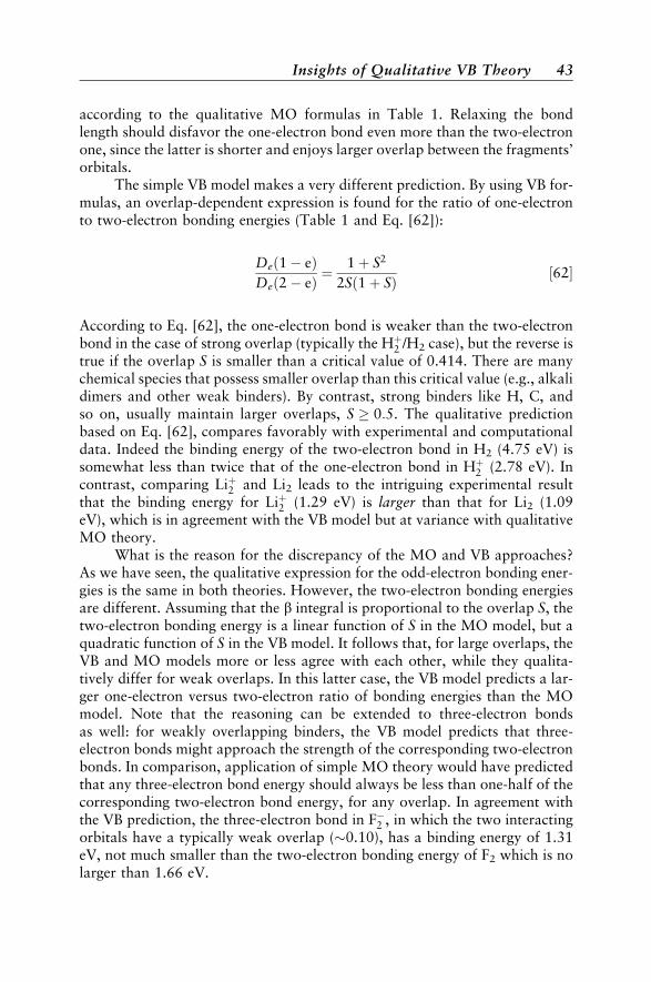
according to the qualitative MO formulas in Table 1. Relaxing the bondlength should disfavor the one-electron bond even more than the two-electronone, since the latter is shorter and enjoys larger overlap between the fragments’orbitals.

The simple VB model makes a very different prediction. By using VB for-mulas, an overlap-dependent expression is found for the ratio of one-electronto two-electron bonding energies (Table 1 and Eq. [62]):

Deð1 eÞDeð2 eÞ ¼

1þ S2

2Sð1þ SÞ ½62�

According to Eq. [62], the one-electron bond is weaker than the two-electronbond in the case of strong overlap (typically the Hþ2 /H2 case), but the reverse istrue if the overlap S is smaller than a critical value of 0.414. There are manychemical species that possess smaller overlap than this critical value (e.g., alkalidimers and other weak binders). By contrast, strong binders like H, C, andso on, usually maintain larger overlaps, S � 0:5. The qualitative predictionbased on Eq. [62], compares favorably with experimental and computationaldata. Indeed the binding energy of the two-electron bond in H2 (4.75 eV) issomewhat less than twice that of the one-electron bond in Hþ2 (2.78 eV). Incontrast, comparing Liþ2 and Li2 leads to the intriguing experimental resultthat the binding energy for Liþ2 (1.29 eV) is larger than that for Li2 (1.09eV), which is in agreement with the VB model but at variance with qualitativeMO theory.

What is the reason for the discrepancy of the MO and VB approaches?As we have seen, the qualitative expression for the odd-electron bonding ener-gies is the same in both theories. However, the two-electron bonding energiesare different. Assuming that the b integral is proportional to the overlap S, thetwo-electron bonding energy is a linear function of S in the MO model, but aquadratic function of S in the VB model. It follows that, for large overlaps, theVB and MO models more or less agree with each other, while they qualita-tively differ for weak overlaps. In this latter case, the VB model predicts a lar-ger one-electron versus two-electron ratio of bonding energies than the MOmodel. Note that the reasoning can be extended to three-electron bondsas well: for weakly overlapping binders, the VB model predicts that three-electron bonds might approach the strength of the corresponding two-electronbonds. In comparison, application of simple MO theory would have predictedthat any three-electron bond energy should always be less than one-half of thecorresponding two-electron bond energy, for any overlap. In agreement withthe VB prediction, the three-electron bond in F2 , in which the two interactingorbitals have a typically weak overlap (�0.10), has a binding energy of 1.31eV, not much smaller than the two-electron bonding energy of F2 which is nolarger than 1.66 eV.


Insight into bonding is not limited to this example. In fact, VB theorygives rise to new bonding paradigms that are discussed in the literature butare not reviewed here for lack of space. One such paradigm is called‘‘charge-shift bonding’’ and concerns two-electron bonds that are neithercovalent nor ionic but whose bonding energy is dominated by the covalent–ionic resonance interaction; for example, FF and OO are charge-shiftbonds.153–155 Another paradigm is the ‘‘ferromagnetic-bonding’’ that occursin high-spin clusters (e.g., nþ1Lin) that are devoid of electron pairs.156,157

VB Diagrams for Chemical Reactivity

One advantage of representing reactions in terms of VB configurations isthe unique and unified insight that it brings to reactivity problems. The center-piece of the VB diagram model is the VB correlation diagram that traces theenergy of the VB configurations along the reaction coordinate. The subsequentconfiguration mixing reveals the cause of the barrier, the nature of the transi-tion state, and the reasons for occurrence of intermediates. Furthermore, thediagram allows qualitative and semiquantitative predictions to be made abouta variety of reactivity problems, ranging from barrier heights, stereo- andregio-selectivities, and mechanistic alternatives. Since its derivation, via theprojection of MO-based wave functions along the reaction coordinate,81 theVB diagram model has been applied qualitatively53,83–85,158 as well as quanti-tatively by direct computation of the VB diagram;159–168 as such this is a qua-litative model with an isomorphic quantitative analogue.

The straightforward representation of the VB diagram focuses on the‘‘active bonds’’, those that are being broken or made during the reaction.Of course, it is the localized nature of the electron pairs in the VB representa-tion that makes this focusing possible. The entire gamut of reactivity phenom-ena requires merely two generic diagrams, which are depicted schematically inFigure 8, and that enable a systematic view of reactivity. The first is a diagramof two interacting states, called a VB state correlation diagram (VBSCD),which describes the formation of a barrier in a single chemical step due toavoided crossing or resonance mixing of the VB states that describe reactantsand products. The second is a three-curve diagram (or generally a many-curvediagram), called a VB configuration-mixing diagram (VBCMD), whichdescribes a stepwise mechanism derived from the avoided crossing and VBmixing of the three curves or more. The ideas of curve crossing and avoidedcrossing were put to use in the early days of VB theory by London, Eyring,Polanyi, and Evans, who pioneered the implementation of VB computationas a means of generating potential energy surfaces and locating transitionstates. In this respect, the VB diagrams (VBSCD and VBCMD) are develop-ments of these early ideas into a versatile system of thought that allows pre-diction of a variety of reactivity patterns from properties of the reactants andproducts.


A review of both kinds of VB diagrams has recently appeared,85 and werefer the reader to this review paper for comprehensive information. Here wewill concentrate on diagrams of the first type, VBSCD, and give a brief accountof their practical use.

The VBSCDs apply to the general category of reactions that can bedescribed as the interplay of two major VB structures, that of the reactants(A/BC in Fig. 8a) and that of the products (AB/C). The diagram displaysthe ground state energy profile of the reacting system (bold curve), as wellas the energy profile of each VB structure as a function of the reaction coordi-nate (thin curves). Thus, starting from the reactant’s geometry on the left, theVB structure that represents the reactant’s electronic state, R, has the lowestenergy and merges with the supersystem’s ground state. Then, as one deformsthe supersystem towards the products’ geometry, the latter VB structure gra-dually rises in energy and finally reaches an excited state P* that represents theVB structure of the reactants in the products’ geometry. A similar diabaticcurve can be traced from P, the VB structure of the products in its optimal geo-metry, to R�, the same VB structure in the reactants’ geometry. Consequently,the two curves cross somewhere in the middle of the diagram. The crossing isof course avoided in the adiabatic ground state, owing to the resonance energyB that results from the mixing of the two VB structures. The barrier is thusinterpreted as arising from avoided crossing between two diabatic curves,which represent the energy profiles of the VB structures of the reactants andproducts.

The VBSCD is a handy tool for making predictions by relating the mag-nitudes of barriers to the properties of reactants. Thus, the barrier �E6¼ of a

Figure 8 The VB diagrams for conceptualizing chemical reactivity: (a) VBSCD showingthe mechanism of barrier formation by avoided crossing of two curves of reactant andproduct type state curves. (b) VBCMD showing the formation of a reaction intermediate.The final adiabatic states are drawn in bold curves.


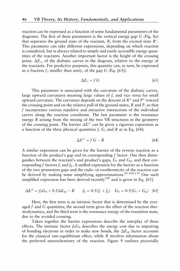
reaction can be expressed as a function of some fundamental parameters of thediagrams. The first of these parameters is the vertical energy gap G (Fig. 8a)that separates the ground state of the reactant, R, from the excited state R�.This parameter can take different expressions, depending on which reactionis considered, but is always related to simple and easily accessible energy quan-tities of the reactants. Another important factor is the height of the crossingpoint, �Ec, of the diabatic curves in the diagram, relative to the energy ofthe reactants. For predictive purposes, this quantity can, in turn, be expressedas a fraction f , smaller than unity, of the gap G (Eq. [63]).

�Ec ¼ f G ½63�

This parameter is associated with the curvature of the diabatic curves,large upward curvatures meaning large values of f, and vice versa for smallupward curvature. The curvature depends on the descent of R* and P* towardthe crossing point and on the relative pull of the ground states, R and P, so thatf incorporates various repulsive and attractive interactions of the individualcurves along the reaction coordinate. The last parameter is the resonanceenergy B arising from the mixing of the two VB structures in the geometryof the crossing point. The barrier �E 6¼ can be given a rigorous expression asa function of the three physical quantities f, G, and B as in Eq. [64]:

�E6¼ ¼ f G B ½64�

A similar expression can be given for the barrier of the reverse reaction as afunction of the product’s gap and its corresponding f factor. One then distin-guishes between the reactant’s and product’s gaps, Gr and Gp, and their cor-responding f factors fr and fp. A unified expression for the barrier as a functionof the two promotion gaps and the endo- or exothermicity of the reaction canbe derived by making some simplifying approximations.85,169,170 One suchsimplified expression has been derived recently168 and is given in Eq. [65].

�E 6¼ ¼ f0G0 þ 0:5�Erp B f0 ¼ 0:5ðfr þ fpÞ G0 ¼ 0:5ðGr þGpÞ ½65�

Here, the first term is an intrinsic factor that is determined by the aver-aged f and G quantities, the second term gives the effect of the reaction ther-modynamics, and the third term is the resonance energy of the transition state,due to the avoided crossing.

Taken together the barrier expressions describe the interplay of threeeffects. The intrinsic factor f0G0 describes the energy cost due to unpairingof bonding electrons in order to make new bonds, the �Erp factor accountsfor the classical rate-equilibrium effect, while B involves information aboutthe preferred stereochemistry of the reaction. Figure 9 outlines pictorially


the impact of the three factors on the barrier. As such, the VB diagram consti-tutes in principle a unified and general structure–reactivity model.

A quantitative application of the diagram requires calculations of either�Ec and B or of f , G, and B. The energy gap factor, G, is straightforward toobtain for any kind of process. The height of the crossing point incorporateseffects of bond deformations (bond stretching, angular changes, etc.) in thereactants and nonbonded repulsions between them at the geometry corre-sponding to the crossing point of the lowest energy on the seam of crossingbetween the two state curves (Fig. 8a). This, in turn, can be computed bymeans of ab initio calculations (e.g., straightforwardly by use of a VBmethod 159,166–168 or with any MO-based method), by determining the energyof the reactant wave function at zero iteration (see Appendix A.3) or by con-strained optimization of block-localized wave functions.171 Alternatively, theheight of the crossing point can be computed by molecular mechanicalmeans.172–174 Except for VB theory that calculates B explicitly, in all othermethods this quantity is obtained as the difference between the energy ofthe transition state and the computed height of the crossing point. In a fewcases, it is possible to use analytical formulas to derive expressions for the

Figure 9 Illustration of the factors that control the variation of the barrier height in theVBSCD.


parameters f and B.53,85,167 Thus, in principle, the VBSCD is computable atany desired accuracy.142

The purpose of this section is to teach an effective way for using the dia-grams in a qualitative manner. The simplest way starts with the G parameter,which is the origin of the barrier, since it serves as a promotion energy neededto unpair the bonds of the reactants and pair the electrons in the moderequired by the products. In certain families of related reactions both the cur-vatures of the diabatic curves (parameter f ) and the avoided crossing reso-nance energy (parameter B) can be assumed to be nearly constant, while inother reaction series f and B vary in the same manner as G. In such cases,the parameter G is the crucial quantity that governs the reaction barriers inthe series: the larger the gap G, the larger the barrier. Let us proceed with afew applications of this type.

Radical Exchange ReactionsFigure 10 describes the VB correlation diagram for a reaction that

involves cleavage of a bond AY by a radical X�(X, A, Y¼ any atom or mole-

cular fragment):

X� þ AY! XAþ Y

� ½66�

Since R� is just the VB image of the product in the geometry of the reactants,this excited state displays a covalent bond coupling between the infinitely

Figure 10 The state correlation in the VBSCD that describes a radical exchangereaction. Avoided crossing as in Figure 8a will generate the final adiabatic profile.


separated fragments X and A, and an uncoupled fragment Y�in the vicinity of

A. The VB wave function of such a state reads (dropping normalizationfactors):

cðR�Þ ¼ j x a y j j x a y j ½67�

where x, a, and y are, respectively, the active orbitals of the fragments X, A, Y.By using the rules of qualitative VB theory (Eqs. [40] and [42] where S2 isneglected), the energy of R� relative to the separated X, A, Y fragmentsbecomes baySay, while the energy of R is just the bonding energy of theAY fragment (i.e., 2baySay). It follows that the energy gap G for any radicalexchange reaction of the type in Eq. [66] is 3baySay, which is just three quar-ters of the singlet–triplet gap �EST of the AY bond, namely,

G � 0:75�ESTðAYÞ ½68�

The state R� in Eq. [67] keeps strictly the wave function of the product P, andis hence a quasi-spectroscopic state that has a finite overlap with R. If oneorthogonalizes the pair of states R and R�, by for example, a Graham–Schmidtprocedure, the excited state becomes a pure spectroscopic state in which theAY is in a triplet state and is coupled to X

�to yield a doublet state. In such

an event, one could simply use, instead of Eq. [68], the gap G0 in Eq. [69] thatis simply the singlet–triplet energy gap of the AY bond:

G0 ¼ �ESTðAYÞ ½69�

Each formulation of the state R� has its own advantages,175 but what is essen-tial for the moment is that both use a gap that is either the singlet–triplet exci-tation of the bond that is broken during the reaction, or the same quantityscaled by approximately a constant 0.75. As mentioned above, a useful wayof understanding this gap is as a promotion energy that is required in orderto enable the AY bond to be broken before it can be replaced by anotherbond, XA.

As an application, let us consider a typical class of radical exchange reac-tions, the hydrogen abstractions from alkanes. Eq. [70] describes the identityprocess of hydrogen abstraction by an alkyl radical:

R� þHR! RHþ R

� ½70�

Identity reactions proceed without a thermodynamic driving force, and projecttherefore the role of promotion energy as the origin of the barrier.

The barriers for a series of radicals have been computed by Yamatakaand Nagase,176 and were found to increase as the RH bond energy D


increases; the barrier is the largest for R¼CH3 and the smallest forR¼C(CH3)3. This trend has been interpreted by Pross et al.177 using theVBSCD model. The promotion gap G that is the origin of the barrier(Eq. [68]) involves the singlet–triplet excitation of the RH bond. Now,according to Eqs. [41] and [42], this singlet–triplet gap is proportional tothe bonding energy of the RH bond, that is, �EST � 2D. Therefore, the cor-relation of the barrier with the bond strength is equivalent to a correlationwith the singlet–triplet promotion energy (Eq. [68]), a correlation that reflectsthe electronic reorganization that is required during the reaction. In fact, thebarriers for the entire series calculated by Pross et al.177 can be fitted very wellto the barrier equation, as follows:

�E6¼ ¼ 0:3481G 50 kcal=mol G ¼ 2DRH ½71�

which indicates that this is a reaction family with constant f ¼ 0:3481 andB ¼ 50 kcal/mol.

Recently, ab initio VB computations demonstrated that the �EST quan-tity167 is the factor that organizes the trends for the barriers for the hydrogenexchange identity reaction, R� þ RH! RHþ� R, when R varies down thecolumn of the periodic table, that is, R ¼ CH3, SiH3, GeH3, and PbH3.Thus, in this series, the barriers decrease down the column since the �EST

quantity decreases.Similar reaction series abound.53,85 Thus, in a series of Woodward–Hoff-

mann forbidden 2þ 2 dimerizations, the promotion gap is proportional to thesum of the �EST (pp�) quantities of the two reactants. Consequently, the bar-rier decreases from 42.2 kcal/mol for the dimerization of ethylene, where��EST (pp�) is large (�200 kcal/mol) down to <10 kcal/mol for the dimeriza-tion of disilene for which ��EST(pp�) is small (�80 kcal/mol). A similar trendwas noted for Woodward–Hoffmann allowed reactions (4þ 2 or 2þ 2þ 2),where the barrier jumps from 22 kcal/mol for the Diels–Alder reaction where��EST(pp�) is small (�173 kcal/mol) to 62 kcal/mol for the trimerization ofacetylene where ��EST(pp�) is very large (�297 kcal/mol).

Reactions between Nucleophiles and ElectrophilesFigure 11 illustrates the formation of the VB correlation diagram for a

reaction between a nucleophile and an electrophile, Eq. [72]:

X þ AY! XAþ Y ½72�

Equation [72] represents a typical SN2 reaction where the nucleophile, X,shifts an electron to the AY electrophile, forms a new XA bond, whilethe leaving group Y departs with the negative charge.

Let us now examine the nature of the R� excited state for this process.Geometrically, A and Y are close together (as in the ground state R) and


separated from X by a long distance. The X fragment, which is neutral in theproduct P, must remain neutral in R�, and therefore carries a single active elec-tron. As a consequence, the negative charge is located on the AY complex, sothat the R� state is the result of a charge transfer from the nucleophile to theelectrophile, and can be depicted as X

�/(A;Y). It follows that the promotion

from R to R� is made of two terms: An electron detachment from the nucleo-phile (e.g., X�

�) and an electron attachment to the electrophile (e.g, AY).

The promotion energy G is therefore the difference between the vertical ioni-zation potential of the nucleophile, I�X��, and the vertical electron affinity of theelectrophile, A�AY, given by Eq. [73],

G ¼ I�X�� A�AY ½73�

where the asterisk denotes a vertical quantity with respect to molecular as wellas solvent configurations.105,106 Thus, the mechanism of a nucleophilic substi-tution may be viewed as an electron transfer from the nucleophile to theelectrophile, and a coupling of the supplementary electron of the electrophileto the remaining electron of the nucleophile.

A whole monograph and many reviews were dedicated to discussion ofSN2 reactivity based on the VBSCD model, and the interested reader mayconsult these.85,169,170,178 One important feature that emerges from these

Figure 11 The state correlation in the VBSCD that describes a nucleophilic substitutionreaction. Avoided crossing as in Figure 8a will generate the final adiabatic profile.


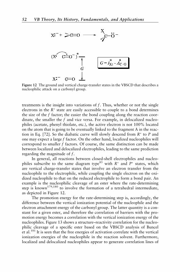
treatments is the insight into variations of f . Thus, whether or not the singleelectrons in the R� state are easily accessible to couple to a bond determinesthe size of the f factor; the easier the bond coupling along the reaction coor-dinate, the smaller the f and vice versa. For example, in delocalized nucleo-philes (acetate, phenyl thiolate, etc.), the active electron is not 100% locatedon the atom that is going to be eventually linked to the fragment A in the reac-tion in Eq. [72]. So the diabatic curve will slowly descend from R� to P andone may expect a large f factor. On the other hand, localized nucleophiles willcorrespond to smaller f factors. Of course, the same distinction can be madebetween localized and delocalized electrophiles, leading to the same predictionregarding the magnitude of f .

In general, all reactions between closed-shell electrophiles and nucleo-philes subscribe to the same diagram type85 with R� and P� states, whichare vertical charge-transfer states that involve an electron transfer from thenucleophile to the electrophile, while coupling the single electron on the oxi-dized nucleophile to that on the reduced electrophile to form a bond pair. Anexample is the nucleophilic cleavage of an ester where the rate-determiningstep is known179,180 to involve the formation of a tetrahedral intermediate,as depicted in Figure 12.

The promotion energy for the rate-determining step is, accordingly, thedifference between the vertical ionization potential of the nucleophile and theelectron attachment energy of the carbonyl group. The latter quantity is a con-stant for a given ester, and therefore the correlation of barriers with the pro-motion energy becomes a correlation with the vertical ionization energy of thenucleophiles. Figure 13 shows a structure–reactivity correlation for the nucleo-philic cleavage of a specific ester based on the VBSCD analysis of Buncelet al.181 It is seen that the free energies of activation correlate with the verticalionization energies of the nucleophile in the reaction solvent. Furthermore,localized and delocalized nucleophiles appear to generate correlation lines of

Figure 12 The ground and vertical charge-transfer states in the VBSCD that describes anucleophilic attack on a carbonyl group.


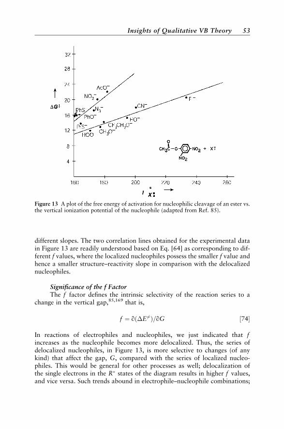
different slopes. The two correlation lines obtained for the experimental datain Figure 13 are readily understood based on Eq. [64] as corresponding to dif-ferent f values, where the localized nucleophiles possess the smaller f value andhence a smaller structure–reactivity slope in comparison with the delocalizednucleophiles.

Significance of the f FactorThe f factor defines the intrinsic selectivity of the reaction series to a

change in the vertical gap,85,169 that is,

f ¼ qð�E6¼Þ=qG ½74�

In reactions of electrophiles and nucleophiles, we just indicated that fincreases as the nucleophile becomes more delocalized. Thus, the series ofdelocalized nucleophiles, in Figure 13, is more selective to changes (of anykind) that affect the gap, G, compared with the series of localized nucleo-philes. This would be general for other processes as well; delocalization ofthe single electrons in the R� states of the diagram results in higher f values,and vice versa. Such trends abound in electrophile–nucleophile combinations;

Figure 13 A plot of the free energy of activation for nucleophilic cleavage of an ester vs.the vertical ionization potential of the nucleophile (adapted from Ref. 85).


they were analyzed for radical addition to olefins,182 and are likely to be a gen-eral feature of reactivity.

Another factor that raises f is the steric bulk of the substrate or thenucleophile.169 For example in SN2 reactions the bulkier the alkyl group inAY (Eq. [72]) the larger will be the value of f , and vice versa.169 As a result,bulkier substrates will exhibit higher sensitivity to changes in the vertical gap.One such variation occurs when the reaction conditions change from gasphase to solution, in which case the promotion gap, G ¼ I�X�� A�AY, increasesby a significant amount. If we now compare two AY substrates suchas methyl chloride and neopentyl chloride, the latter will possess a larger fvalue. The consequence is that the steric effect that is observed in the gas phasewill be amplified and become more significant in a solvent. This excitingfinding was recently published by Ren and Brauman.183

Making Stereochemical Predictions with the VBSCD ModelMaking stereochemical predictions is easy using FO–VB configura-

tions.52,81,85 To illustrate the manner by which this can be practiced, let ustake a simple example with well-known stereochemistry, the nucleophilic sub-stitution reaction, Eq. [72]. The corresponding R� state is depicted in Figure 14in its FO–VB formulation, where the nucleophile appears here in its one-electron reduced form X

�, with a single electron in fX, while the substrate

has an extra electron in its s�CY orbital. The two single electrons are coupledinto a fX s�CY bond pair.

The R� state correlates to product, XC/:Y, since it contains afX s�CY bond-pair that becomes the XC bond, and at the same time theoccupancy of the s�CY orbital causes the cleavage of the CY bond to release

Figure 14 The ground (R) and charge-transfer (R�) states in the VBSCD of the SN2reaction X þ C Y! X Cþ Y. The R� state has a bond pair shown by the lineconnecting the orbitals fx and s�cy.


the: Y anion. Furthermore, the R� state contains information about thestereochemical pathway. Since the bond pair involves a fX s�CY overlap,due to the nodal properties of the s�CY orbital the bond pair will be optimizedwhen the X

�is coupled to the substrate in a colinear XCY fashion. Thus,

the steepest descent of the R� state, and the lowest crossing point will occuralong a backside trajectory of the nucleophile toward the substrate.

If we assume that the charge-transfer state remains the leading configura-tion of R� near the crossing point, then the matrix element between R and R�

will dominate the size of the resonance energy B, and will enable making pre-dictions about B. Since these two VB configurations differ by the occupancy ofone spin orbital (fX in R is replaced by s�CY in R�) then following the quali-tative rules for matrix elements (see Appendix A.2), the resonance energy ofthe transition state (TS) will be proportional to the overlap of these orbitals,that is,

B / hfXjs�CYi ½75�

It follows therefore, that in a backside trajectory, we obtain both the lowestcrossing point as well as the largest TS resonance energy. Computationally,the back-side barrier is smaller by �10–20 kcal/mol compared with a front-side attack.184 Equation [75] constitutes an orbital selection rule for an SN2reaction. Working out this rather trivial prediction is nevertheless necessarysince it constitutes a prototypical example for deriving orbital selection rulesin other reactions, using FO–VB configurations. Thus, the intrinsic bondingfeatures of R� provide information about the reaction trajectory, while thehRjR�i overlap provides information about the geometric dependence of theresonance energy of the TS, B.

By using this approach, it is possible to derive orbital selection rules forcases that are ambiguous in qualitative MO theory. For example, for radicalcleavage of s bonds, using the R� with a triplet s1 s�1 configuration on thesubstrate leads to prediction that the course of the reaction and the resonanceinteraction in the transition state will be determined by the product of overlapsbetween the orbital of the attacking radical, fR, and the s and s� orbitals ofthe substrate, namely, hfRjsihfRjs�i. This product is optimized once again ina back-side attack, and therefore one can predict that radical cleavage of sbonds will proceed with inversion of configuration. All known experimentaldata185–190 conform to this prediction. Another area where successful predic-tions have been made involves nucleophilic attacks on radical cations. Hereusing the corresponding R and R� states,191 it was predicted that stereoselec-tivity and regioselectivity of nucleophilic attack should be controlled by thelowest unoccupied molecular orbital (LUMO) of the radical cation. Both regio-selectivity and stereospecificity predictions were verified by experiment192,193

and computational means.184 For a more in depth discussion the reader mayconsult the most recent review of the VBSCD and VBCMD models.85


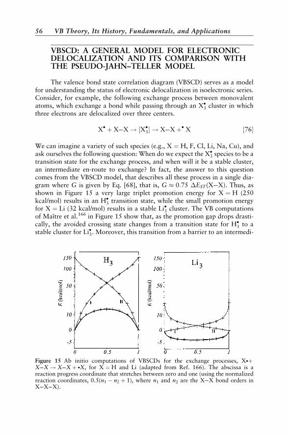
VBSCD: A GENERAL MODEL FOR ELECTRONICDELOCALIZATION AND ITS COMPARISON WITHTHE PSEUDO-JAHN–TELLER MODEL

The valence bond state correlation diagram (VBSCD) serves as a modelfor understanding the status of electronic delocalization in isoelectronic series.Consider, for example, the following exchange process between monovalentatoms, which exchange a bond while passing through an X�3 cluster in whichthree electrons are delocalized over three centers.

X� þXX! ½X�3� ! XXþ� X ½76�

We can imagine a variety of such species (e.g., X ¼ H, F, Cl, Li, Na, Cu), andask ourselves the following question: When do we expect the X�3 species to be atransition state for the exchange process, and when will it be a stable cluster,an intermediate en-route to exchange? In fact, the answer to this questioncomes from the VBSCD model, that describes all these process in a single dia-gram where G is given by Eq. [68], that is, G � 0:75 �EST(XX). Thus, asshown in Figure 15 a very large triplet promotion energy for X ¼ H (250kcal/mol) results in an H�3 transition state, while the small promotion energyfor X ¼ Li (32 kcal/mol) results in a stable Li�3 cluster. The VB computationsof Maıtre et al.166 in Figure 15 show that, as the promotion gap drops drasti-cally, the avoided crossing state changes from a transition state for H�3 to astable cluster for Li�3. Moreover, this transition from a barrier to an intermedi-

Figure 15 Ab initio computations of VBSCDs for the exchange processes, X�þXX! XXþ �X, for X ¼ H and Li (adapted from Ref. 166). The abscissa is areaction progress coordinate that stretches between zero and one (using the normalizedreaction coordinates, 0.5(n1 n2 þ 1), where n1 and n2 are the XX bond orders inXXX).


ate can in fact be predicted quantitatively from the barrier equation, by deriv-ing explicit expressions for G, f , and B.167

The spectacular relationship between the nature of the X�3 species and thepromotion energy shows that the VBSCD is in fact a general model ofthe pseudo-Jahn–Teller effect (PJTE). A qualitative application of PJTE wouldpredict all the X�3 species to be transition state structures that relax to the dis-torted X�XX and XX�X entities. The VBSCD makes a distinctionbetween strong binders that form transition states and weak binders thatform stable intermediate clusters.

The variable nature of the X�3 species in the isoelectronic series form ageneral model for electronic delocalization, enabling one to classify the specieseither as distortive or as stable. By using the isoelectronic analogy, one mightnaturally ask about the isoelectronic p-species in allyl radical; does it behaveby itself like H�3 or like Li�3? Moreover, the same transformation displayed forX�3 in Figure 15 can be shown for Xþ3 , X3 , X4, and X6 species.57 Likewise onemight wonder about the status of the corresponding isoelectronic p compo-nents in allyl cation, anion, cyclobutadiene, or benzene. These questionswere answered in detail elsewhere and the reader is advised to consult a recentreview,57 while here we deal only with the intriguing question concerning thep-electrons of benzene.

What Is the Driving Force, s or p, Responsible for theD6h Geometry of Benzene?

The regular hexagonal structure of benzene can be considered as a stableintermediate in a reaction that interchanges two distorted Kekule-type iso-mers, each displaying alternating CC bond lengths as shown in Figure 16.It is well known that the D6h geometry of benzene is stable against a Kekuleandistortion (of b2u symmetry), but one may still wonder which of the two sets ofbonds, s or p, is responsible for this resistance to a b2u distortion. The sframe, which is just a set of identical single bonds, is by nature symmetrizingand prefers a regular geometry. It is not obvious whether the p electronic com-ponent, by itself, is also symmetrizing or on the contrary distortive, with aweak force constant that would be overwhelmed by the symmetrizing drivingforce of the s frame. To answer this question, consider in Figure 16 theVBSCD that represents the interchange of Kekule structures along the b2u

reaction coordinate; the middle of the b2u coordinate corresponds to theD6h structure, while its two extremes correspond to the bond-alternatedmirror-image Kekule geometries. Part a of the figure considers p energiesonly. Starting at the left-hand side, Kekule structure K1 correlates to theexcited state K�2 in which the p bonds of the initial K1 structure are elongated,while the repulsive nonbonding interactions between the p bonds are rein-forced. The same argument applies if we start from the right-hand side,with structure K2 and follow it along the b2u coordinate; K2 will then rise

VBSCD: A General Model for Electronic Delocalization 57

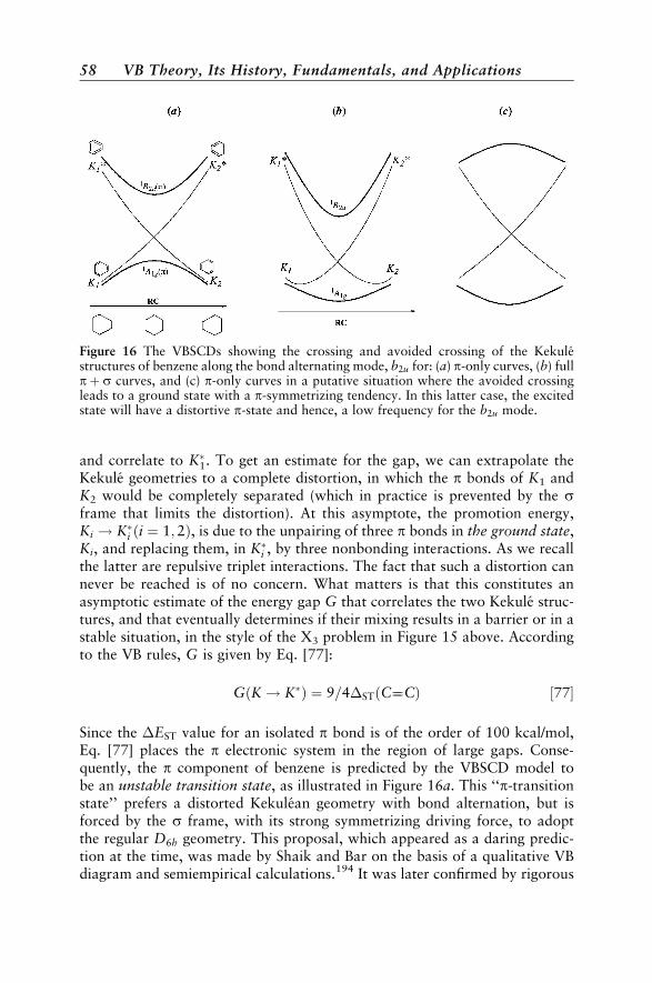
and correlate to K�1. To get an estimate for the gap, we can extrapolate theKekule geometries to a complete distortion, in which the p bonds of K1 andK2 would be completely separated (which in practice is prevented by the sframe that limits the distortion). At this asymptote, the promotion energy,Ki ! K�i ði ¼ 1;2Þ, is due to the unpairing of three p bonds in the ground state,Ki, and replacing them, in K�i , by three nonbonding interactions. As we recallthe latter are repulsive triplet interactions. The fact that such a distortion cannever be reached is of no concern. What matters is that this constitutes anasymptotic estimate of the energy gap G that correlates the two Kekule struc-tures, and that eventually determines if their mixing results in a barrier or in astable situation, in the style of the X3 problem in Figure 15 above. Accordingto the VB rules, G is given by Eq. [77]:

GðK! K�Þ ¼ 9=4�STðCCÞ ½77�

Since the �EST value for an isolated p bond is of the order of 100 kcal/mol,Eq. [77] places the p electronic system in the region of large gaps. Conse-quently, the p component of benzene is predicted by the VBSCD model tobe an unstable transition state, as illustrated in Figure 16a. This ‘‘p-transitionstate’’ prefers a distorted Kekulean geometry with bond alternation, but isforced by the s frame, with its strong symmetrizing driving force, to adoptthe regular D6h geometry. This proposal, which appeared as a daring predic-tion at the time, was made by Shaik and Bar on the basis of a qualitative VBdiagram and semiempirical calculations.194 It was later confirmed by rigorous

Figure 16 The VBSCDs showing the crossing and avoided crossing of the Kekulestructures of benzene along the bond alternating mode, b2u for: (a) p-only curves, (b) fullpþ s curves, and (c) p-only curves in a putative situation where the avoided crossingleads to a ground state with a p-symmetrizing tendency. In this latter case, the excitedstate will have a distortive p-state and hence, a low frequency for the b2u mode.


ab initio calculations, using different techniques of s–p separations, by thepresent authors and their co-workers195–198 and by others.199–202 It wasfurther linked, by the work of Haas and Zilberg,203 to experimental data asso-ciated with the vibrational frequencies of the excited states of benzene.

The experimental data discussed by Haas and Zilberg,203 as well as thoseof pioneering assignments204–206 show a peculiar phenomenon. This phenom-enon is both state specific to the 1B2u excited state, as well as vibrationallymode specific, to the bond-alternating mode, that is, the Kekule mode b2u.Thus, upon excitation from the 1A1g ground state to the 1B2u excited state,with exception of b2u all other vibrational modes behave ‘‘normally’’ andundergo frequency lowering in the excited state, as expected from the decreasein p bonding and disruption of aromaticity following a p!p� excitation. Bycontrast, the Kekule b2u mode, undergoes an upward shift of 257–261 cm1.As explained below, this phenomenon is predictable from the VBSCD modeland constitutes a critical test of p distortivity in the ground state of benzene.

Indeed, the VBSCD model is able to lead to predictions not only on theground state of an electronic system, but also on some selected excited state.Thus, the mixing of the two Kekule structures K1 and K2 in Figure 16a leads toa pair of resonant and antiresonant states K1 � K2; the 1A1g ground stateK1 þ K2 is the resonance-stabilized combination, and the 1B2u excited stateK1 K2 is the antiresonant mixture (this is the first excited state of ben-zene207). In fact, the VBSCD in Figure 16a predicts that the curvature of the1A1g(p) ground state (restricted to the p electronic system) is negative, whereasby contrast, that of the 1B2u(p) state is positive. Of course, when the energy ofthe s frame is added as shown in Figure 16b, the net total driving force for theground state becomes symmetrizing, with a small positive curvature. By com-parison, the 1B2u excited state displays now a steeper curve and is much moresymmetrizing than the ground state, having more positive curvature. As such,the VBSCD model predicts that an 1A1g!1B2u excitation of benzene shouldresult in the reinforcement of the symmetrizing driving force, which will bemanifested as a frequency increase of the Kekulean b2u mode. We may consideran alternative scenario, displayed in Figure 16c where now we assume thatthe p component for the ground state is symmetrizing (positive curvature) asmight have been dictated by common wisdom. In such an event, the p compo-nent would be distortive in the 1B2u state, and consequently, the excitationwould have resulted in the lowering of the b2u frequency. Since this is clearlynot the case, the finding of an enhanced b2u frequency in the excited stateconstitutes an experimental proof of the p distortivity in the ground state ofbenzene.

In order to show how delicate the balance is between the s and p oppos-ing tendencies, we recently57 derived an empirical equation, Eq. [78], for4nþ 2 annulenes:

�Epþs ¼ 5:0ð2nþ 1Þ 5:4ð2nÞ kcal=mol ½78�

VBSCD: A General Model for Electronic Delocalization 59

Here �Epþs stands for the total (p and s) distortion energies, the terms5.0(2nþ 1) represent the resisting s effect, which is 5.0 kcal/mol for an adja-cent pair of s bond, whereas the negative term, 5.4(2n), accounts for the pdistortivity. This expression predicts that for n ¼ 7, namely, the C30H30 annu-lene, the �Epþs becomes negative and the annulene undergoes bond localiza-tion. If we increase the p distortivity coefficient a tiny bit, namely, to

�Epþs ¼ 5:0ð2nþ 1Þ 6:0ð2nÞ kcal=mol ½79�

the equation would now predict that the annulene with n ¼ 3, namely,C14H14, will undergo bond localization. This extreme sensitivity, which is pre-dicted to manifest in computations and experimental data of annulenes, is asimple outcome of the VBSCD prediction that the p component of these spe-cies behaves as a transition state with a propensity toward bond localization.

VBSCD: THE TWIN-STATE CONCEPT AND ITS LINKTO PHOTOCHEMICAL REACTIVITY

Photochemistry is an important field for future applications. The pio-neering work of van Der Lugt and Oosterhoff89 and Michl91 highlighted theimportance of avoided crossing regions as decay channels in photochemistry.Koppel and co-workers208,209 showed that conical intersections, rather thanavoided crossing regions, are the most efficient decay channels, from excitedto ground states. Indeed, this role of conical intersections in organic photo-chemistry has been extensively investigated by Robb and co-workers,93,96

and conical intersections are calculated today on a routine basis using softwaresuch as GAUSSIAN. Bernardi et al.93 further showed that VB notions can beuseful to rationalize the location of conical intersections and their structure.

As was subsequently argued by Shaik and Reddy,97 the VBSCD is astraightforward model for discussing the relation between thermal and photo-chemical reactions and between the avoided crossing region and a conicalintersection. Thus, the avoided crossing region of the VBSCD leads to thetwin-states �z and �� (Fig. 17); one corresponds to the resonant state of theVB configurations and the other to the antiresonant state.85 Since the extent ofthis VB mixing is a function of geometry, there should exist in principle, a spe-cific distortion mode that converts the avoided crossing region into a conicalintersection where the twin-states �z and �� become degenerate, and therebyenable the excited reaction complex to decay into the ground-state surface. Inthis manner, the conical intersection will be anchored at three structures; twoof them are the reactant (R) and product (P1) of the thermal reaction, andthe third is the product (P2) generated by the distortion mode that causesthe degeneracy of the twin-states �z and ��. The new product would therefore


be characteristic of the distortion mode that is required to convert the avoidedcrossing region into a conical intersection. Assuming that most of the excitedspecies roll down eventually to the �� funnel, then P2 would be a major photo-product.a

A trivial example is the celebrated hydrogen exchange reaction,Ha Hb þHc ! Ha þHb Hc, where the transition state has a colinear geo-metry, Ha Hb Hc. In this geometry, the ground state �z is the resonatingcombination of R and P and the transition state for the thermal reaction, whilethe twin-excited state �* is the corresponding antiresonating combination:

�z ¼ R P;

R ¼ jabcj jabcj P ¼ jabcj jabcj ½80�� ¼ Rþ P ¼ jabcj jabcj ½81�

where the orbitals a, b, and c belong to Ha, Hb, and Hc, respectively.It is clear from Eq. [81] that �� involves a bonding interaction between

Ha and Hc and will be lowered by the bending mode that brings Ha and Hc

together. Furthermore, the expression for the avoided crossing interaction B(Eq. [82]) shows that this quantity shrinks to zero in an equilateral triangular

B ¼ hRjHeffjPi ¼ 2babSab 2bbcSbc þ 4bacSac ½82�

Figure 17 (a) The VBSCD showing the twin-states formed by avoided crossing along thereaction coordinate of the thermal reaction leading to product P1. (b) The crossover ofthe twin-states to generate a conical intersection (CI) along a coordinate that stabilizesthe twin excited state, and leading to product P2. (c) The conical intersection will beanchored in three minima (or more): reactants (R), P1, and P2.

a If, however, there exist other excited-state funnels near the twin excited state, ��, other

products will be formed, which are characteristic of these other excited states and can be predicted

in a similar manner provided one knows the identity of these excited states.

VBSCD: The Twin-State Concept 61

structure where the HaHc, HaHb, and HbHc interactions are identical.As such, the equilateral triangle defines a conical intersection with a doublydegenerate state, in the crossing point of the VBSCD. This D3h structurewill relax to the isosceles triangle with short HaHc distance that will giverise to a ‘‘new’’ product HbþHaHc. The photocyclization of allyl radicalto cyclopropyl radical is precisely analogous. The ground state of allyl is theresonating combination of the two Kekule structures, while the twin-excitedstate, ��, is their antiresonating combination with the long bond betweenthe allylic terminals.52 As such, rotation of the two allylic terminals will lower��, raise the ground state, and establish a conical intersection that will channelthe photoexcited complex to the cyclopropyl radical, and vice versa.

The photostimulation of SN2 systems such as X þ AY (A ¼ Alkyl)was analyzed before, using VBSCD-based rationale, for predicting the locationof conical intersections.97 Here, the transition state for the thermal reaction isthe colinear [XAY] structure, which is the �6¼(A0) resonating combinationof the two Lewis structures, while the twin-excited state, ��(A00), is their anti-resonating combination; the symmetry labels refer to Cs symmetry. This latterexcited state is readily written as an A00 symmetry-adapted combination ofLewis structures, Eq. [83]:

�� ¼ ðj xx ay j j xx a y jÞ ðj yy x a j j yy x a jÞ ½83�

where the orbitals x, a, and y belong to the fragments X, A, and Y, respec-tively.

Rearranging Eq. [83] to Eq. [84] reveals a stabilizing three-electronbonding interaction between X and Y, of the type (X� ��Y ! X��

�YÞ:

�� ¼ ðj x xy a j þ j x yy a jÞ ðj xx ya j þ jxy ya jÞ ½84�

As such, the bending mode that brings the X and Y groups together destabi-lizes the [XAY] structure and stabilizes the twin-excited state, until theyestablish a conical intersection that correlates down to X;Y and R�, asshown in Figure 18. This analysis is supported by experimental observationthat the irradiation of the I/CH3I cluster at the charge-transfer band leadsto I2 and CH�3, while for I/ CH3Br such excitation generates IBr andCH�3.210

The notion of twin-states of the VBSCD and the phase inversion rule ofLonguet–Higgins were utilized by Zilberg and Haas98 to delineate unifiedselection rules for conical intersections, and rationalize the outcome of a vari-ety of photochemical reactions.

The presence of excited-state minima above the thermal transition stateis a well known phenomenon.89,91–93 The VBSCD model merely gives this ubi-quitous phenomenon a simple mechanism in terms of the avoided crossing of


VB structures, and hence enables one to make predictions in a systematic man-ner. Other important applications of the twin states concern the possibility ofspectroscopic probing or accessing the twin excited state that lies directlyabove the transition state of a thermal reaction. Thus, much like the foregoingstory of benzene, any chemical reaction will possess a transition state, �z and atwin excited state, ��.81,211 For most cases, albeit not all, the twin excitedstate should be stable, and hence observable; its geometry will be almost co-incident with the thermal transition state and its electronic state symmetryshould be identical to the symmetry of the reaction coordinate of theground-state process,212 namely,

ð��Þ ¼ ðQRCÞ ½85�

In addition, the twin excited state will possess a real and greatly increased fre-quency of the reaction coordinate mode, by analogy to the benzene storywhere the b2u mode was enhanced in the 1b2u twin excited state. Thus, sincethe twin pair has coincident geometry, a spectroscopic characterization of ��

will provide complementary information on the transition state �z and willenable resolution of the transition state structure.

Figure 18 Generation of a conical intersection (CI) by crossing of the twin statesalong the bending distortion mode, in SN2 systems. Symmetry labels refer to the mirrorplane m.

VBSCD: The Twin-State Concept 63

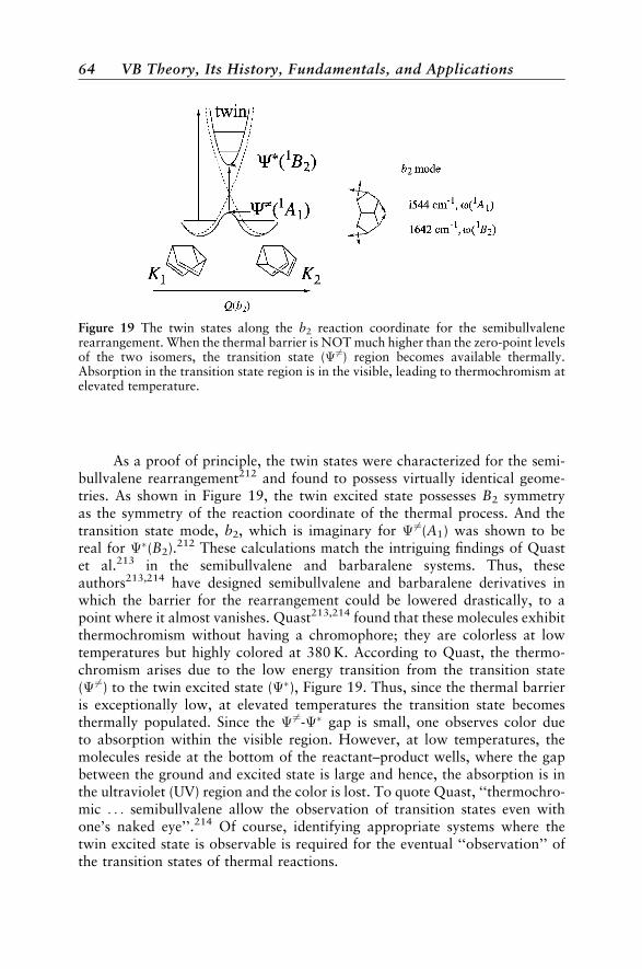
As a proof of principle, the twin states were characterized for the semi-bullvalene rearrangement212 and found to possess virtually identical geome-tries. As shown in Figure 19, the twin excited state possesses B2 symmetryas the symmetry of the reaction coordinate of the thermal process. And thetransition state mode, b2, which is imaginary for � 6¼(A1) was shown to bereal for ��(B2).212 These calculations match the intriguing findings of Quastet al.213 in the semibullvalene and barbaralene systems. Thus, theseauthors213,214 have designed semibullvalene and barbaralene derivatives inwhich the barrier for the rearrangement could be lowered drastically, to apoint where it almost vanishes. Quast213,214 found that these molecules exhibitthermochromism without having a chromophore; they are colorless at lowtemperatures but highly colored at 380 K. According to Quast, the thermo-chromism arises due to the low energy transition from the transition state(�6¼) to the twin excited state (��), Figure 19. Thus, since the thermal barrieris exceptionally low, at elevated temperatures the transition state becomesthermally populated. Since the � 6¼-�� gap is small, one observes color dueto absorption within the visible region. However, at low temperatures, themolecules reside at the bottom of the reactant–product wells, where the gapbetween the ground and excited state is large and hence, the absorption is inthe ultraviolet (UV) region and the color is lost. To quote Quast, ‘‘thermochro-mic . . . semibullvalene allow the observation of transition states even withone’s naked eye’’.214 Of course, identifying appropriate systems where thetwin excited state is observable is required for the eventual ‘‘observation’’ ofthe transition states of thermal reactions.

Figure 19 The twin states along the b2 reaction coordinate for the semibullvalenerearrangement. When the thermal barrier is NOT much higher than the zero-point levelsof the two isomers, the transition state (� 6¼) region becomes available thermally.Absorption in the transition state region is in the visible, leading to thermochromism atelevated temperature.


Coherent control215 is a powerful new chemical method that makes useof the availability of the twin excited state to control the course of chemicalreactions by laser excitation. Thus, laser excitation from �z to ��(Fig. 17a),using two different and complementary photons causes the decay of �� tooccur in a controlled manner either to the reactant or products. In the casewhere the reactants and products are two enantiomers, the twin excited stateis achiral, and the coherent control approach leads to chiral resolution.

In summary, the twin excited state plays an important role in photo-chemistry as well as in thermal chemistry.

THE SPIN HAMILTONIAN VB THEORY

Quite a different brand of VB theory comes from physics, and is rootedin the phenomenological Hamiltonians that are called magnetic- or spin-Hamiltonians after their first formulation by Heisenberg.9 Unlike the theoryused above, which relies on VB structures that are eigenfunctions of boththe Sz and S2 operators, this theory relies on VB determinants, which are eigen-functions of only the Sz operator. The following section describes the type ofinsight that can be gained from this VB approach.

Theory

The spin-Hamiltonian VB theory uses the same approximations as thequalitative theory presented above to calculate the Hamiltonian matrix ele-ments, but with a few simplifications. The theory is restricted to determinantshaving one electron per AO; this restriction excludes ionic structures or mole-cules bearing lone pairs. As such, the theory has mainly been applied to con-jugated polyenes. Another simplification is the zero-differential overlapapproximation, which means that all overlaps are neglected in the formulas.

Apart from these simplifying assumptions, a fundamental differencebetween qualitative VB theory and spin-Hamiltonian VB theory is that thebasic constituent of the latter theory is the AO determinant, without any apriori bias for a given electronic coupling into bond pairs. Instead of an inter-play between VB structures, a molecule is viewed then as a collective spin-ordering: The electrons tend to occupy the molecular space (i.e., the variousatomic centers) in such a way that an electron of a spin will be surroundedby as many b spin electrons as possible, and vice versa. Determinants havingthis property, called the ‘‘most spin-alternated determinants’’ (MSAD) havethe lowest energies (by virtue of the VB rules, in Qualitative VB Theory)and play the major role in electronic structure. As a reminder, the readershould recall from our discussion above that the unique spin-alternant deter-minant, which we called the quasiclassical state, is used as a reference for theinteraction energy.

The Spin Hamiltonian VB Theory 65

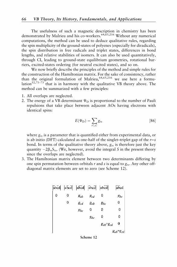
The usefulness of such a magnetic description in chemistry has beendemonstrated by Malrieu and his co-workers.64,65,216 Without any numericalcomputations, the method can be used to deduce qualitative rules, regardingthe spin multiplicity of the ground-states of polyenes (especially for diradicals),the spin distribution in free radicals and triplet states, differences in bondlengths, and relative stabilities of isomers. It can also be used quantitatively,through CI, leading to ground-state equilibrium geometries, rotational bar-riers, excited-states ordering (for neutral excited states), and so on.

We now briefly describe the principles of the method and simple rules forthe construction of the Hamiltonian matrix. For the sake of consistency, ratherthan the original formulation of Malrieu,64,65,216 we use here a formu-lation52,71–73 that is in harmony with the qualitative VB theory above. Themethod can be summarized with a few principles:

1. All overlaps are neglected.2. The energy of a VB determinant �D is proportional to the number of Pauli

repulsions that take place between adjacent AOs having electrons withidentical spins:

Eð�DÞ ¼Xr";s"

grs ½86�

where grs is a parameter that is quantified either from experimental data, oris ab initio (DFT) calculated as one-half of the singlet–triplet gap of the rsbond. In terms of the qualitative theory above, grs is therefore just the keyquantity 2brsSrs. (We, however, avoid the integral S in the present theorysince the overlaps are neglected).

3. The Hamiltonian matrix element between two determinants differing byone spin permutation between orbitals r and s is equal to grs. Any other off-diagonal matrix elements are set to zero (see Scheme 12).

Scheme 12


Diagonalization of this matrix gives the energy of the ground state relative tothe nonbonding state (the spin-alternant determinant), and in addition leads tothe entire spectrum of the lowest neutral excited states. Note that applying thespin-Hamiltonian model to ethylene leads to a p bonding energy g, which isequivalent to the 2bS used in the qualitative VB theory above.

Applications

Ground States of Polyenes and Hund’s Rule ViolationsA simple principle of the spin-Hamiltonian VB theory is that the lowest

state of a molecule will have the multiplicity associated with the Sz value of itsMSAD, that is, it will be a singlet if na ¼ nb in the MSAD, a doublet if na ¼nb þ 1, a triplet if na ¼ nb þ 2, and so on.217 For example, the MSAD oforthoxylylene 27 and paraxylylene 28 (Scheme 13) both have Sz ¼ 0 whilethat of metaxylylene (29) has Sz ¼ 1.

It follows that ortho- and para-xylylenes will have singlet ground stateswhile metaxylylene has a triplet ground state. The prediction is correct but notparticularly surprising, since 27 and 28 can be described by a perfectly pairedKekule structure while 29 cannot and is therefore a diradical that will be a tri-plet state based on Hund’s rule. More intriguing are the predictions of Hund’srule violations. Let us consider, for example, 2,3-dimethylene-butadiene and1,3-dimethylene-butadiene.These are two polyenes for which it is impossibleto draw a Kekule structure, and which are therefore diradicaloids. Now theMSAD of these two species (30 and 31 in Scheme 14) have different Sz values,Sz ¼ 0 for 30 versus Sz ¼ 1 for 31.

Scheme 13

Scheme 14

The Spin Hamiltonian VB Theory 67

In this case, the spin-Hamiltonian predicts 2,3-dimethylene-butadiene tobe a singlet diradicaloid (in violation of Hund’s rule) and 1,3-dimethylene-butadiene to be a triplet, in agreement with experiment. By contrast, monode-terminantal MO calculations predict that all these diradicaloids have tripletground states. It is only after CI that one gets the correct assignments.218 Vio-lations of Hund’s rule can be explained by the phenomenon of dynamic spin-polarization and predicted to take place when the degenerate singly occupiedMOs form a disjointed set.218,219 In such a case, the advantage of the tripletover the singlet becomes very weak owing to a small exchange integral, andwhen CI is applied, it preferentially stabilizes the singlet, and reverses the singlet–triplet energy order. Comparison of the spin-polarization argument to the pre-sent VB analysis, shows the VB method to be faster, physically intuitive, andindependent of any numerical calculation.

Relative Stabilities of PolyenesSubtle predictions can be made about the relative energies of two isomers

having comparable Kekule structures, such as the linear s-trans conformationand branched conformation of hexatriene, 18 and 22 in Scheme 9 above. Foreach of these isomers, we shall consider that the total p energy is a perturbation of

the energy of the MSAD (e.g., 32 for the linear conformation in Scheme 15) byless ordered determinants. Each of the latter determinants is generated fromthe MSAD by the inversion of two spins along a given linkage (e.g., 33 vs.32 in Scheme 15), while keeping the total Sz constant. According to the aboverules, the Hamiltonian matrix element between 32 and 33 is the integral gbc,and the energy of 32 relative to 33 is gab þ gcd, since the spin reorganizationintroduces two Pauli repulsions along the a-b and c-d linkages.

More generally, the number of Pauli repulsions that one introduces, rela-tive to the MSAD, by inverting the spins in a linkage r-s is equal to the numberof linkages that are adjacent to r-s. Thus, assuming that all the g integrals arethe same for the sake of simplicity, the energy of a determinant �rs generatedby spin inversion relative to a MSAD � is given by Eq. [87]:

EðcrsÞ EðcÞ ¼ g� naðrsÞ ½87�

Scheme 15


where na is the number of linkages that are adjacent to r-s. We now considerall determinants displaying a spin transposition between two adjacent atomswith respect to the MSAD. The matrix elements between the determinants �rs

and � will be the same and all equal to the g integral. Hence, the total p energythat arises from a second order perturbation correction (PT2) will be given byEq. [88]:

EðPT2Þ ¼X

rs

g2

gnaðrsÞ¼ g

Xrs

1

naðrsÞ½88�

where the energy is calculated relative to the MSAD. Therefore, it appears thatthe energy of a polyene is a simple topological function that is related to theshape of the molecule and to the way the various linkages are connected toeach other. Calculating the energies of the two isomers of hexatriene is thus

a simple matter. In Scheme 16, each linkage in 34 and 35 is labeled by thenumber of bonds that are adjacent it. From these numbers, the expressionsfor the total energies of each isomer are immediately calculated (Scheme16), and clearly show that the linear isomer is more stable than the branchedone, in agreement with experimental facts.

AB INITIO VB METHODS

A number of ab initio VB methods have been implemented to calculateVB wave functions and their associated energies and molecular properties.Once the general scheme for writing VB wave functions is established (seeBasic VB Theory above), an important task is the optimization of the orbitalsthat are used to construct the AO or FO determinants of the VB structures.Historically, the classical VB method used the atomic orbitals of the freeatoms, without any further change. This crude approximation, which is nolonger employed, resulted in highly inaccurate energies, since it does nottake into account the considerable rearrangements in size and shape that an

Scheme 16

Ab Initio VB Methods 69

AO undergoes when fragments assemble to a molecule. Accordingly, weshall restrict ourselves here to modern VB methods that perform orbitaloptimization.

Orbital-Optimized Single-Configuration Methods

A great step forward in accuracy and compactness was made when opti-mized orbitals of Coulson–Fischer (CF) type were employed in VB calcula-tions. As shown above (Basic VB Theory), describing a two electron bondas formally covalent singlet coupling between two CF orbitals ja and jb

(Eqs. [6b] and [6c]), which are optimized and free to delocalize over thetwo centers, is an ingenious way to include both the covalent and ionic com-ponents of the bond in an implicit way in a wave function of the Heitler–London type. Thus, the CF representation has the advantage of keepingthe well-known picture of perfect pairing while treating the left–right electroncorrelation associated with any given bond in a variational way.

The CF proposal, generalized to polyatomic molecules, gave rise to the‘‘separated electron pair’’ theory that was initiated by Hurley et al.220 andlater developed as the GVB method by Goddard and co-workers,109,221,222

and as the SC method by Gerratt and co-workers.112–114,223–225 In both theselatter methods the valence electrons are described by a single configuration ofsingly occupied orbitals, and the various spin-coupled structures—generatedso as to form a complete and linearly independent set of spin-eigenfunc-tions—are allowed to mix to generate the final state. In the SC method,both the orbitals and the mixing coefficients are optimized simultaneously,while in the most general form of GVB theory they are optimized sequentially.It is important to note that, while no constraint of any kind is applied to theshapes of the orbitals during the optimization, they are generally obtainedin a form that is pretty much localized, as will be exemplified below. Thus,each bond in a polyatomic VB structure is viewed as a pair of singlet-coupledorbitals that are quasi-atomic and display a strong mutual overlap.

The Generalized VB MethodThe GVB method is generally used in its restricted perfectly paired form,

referred to as GVB–PP, which pairs the atoms as in the most important Lewisstructure. The GVB–PP method introduces two simplifications. The first one isthe Perfect-Pairing (PP) approximation, by which only one VB structure is gen-erated in the calculation. The wave function may then be expressed in the sim-ple form of Eq. [89], where each term in parentheses is a so-called ‘‘geminal’’two-electron function, which takes the form of a singlet-coupled GVB pair(jia, jib) and is associated with one particular bond or lone pair.

cGVB ¼ j ðj1aj1b j1aj1bÞðj2aj2b j2aj2bÞ � � � ðjnajnb jnajnbÞ j ½89�


The second simplification, which is introduced for computational conve-nience, is the strong orthogonality constraint, whereby all the orbitals inEq. [89] are required to be orthogonal to each other unless they are singletpaired, that is,

hjiajjibi 6¼ 0 ½90a�

hjijjji ¼ 0 otherwise ½90b�

This strong orthogonality constraint is, of course, a restriction, however,usually not a serious one, since it applies to orbitals that are not expected tooverlap significantly. By contrast, the orbitals that are coupled together in agiven GVB pair display, of course, a strong overlap.

For further mathematical convenience, each geminal in Eq. [89] can berewritten, by simple orbital rotation, as an expansion in terms of natural orbi-tals,

j ðj1aj1b j1aj1bÞ j ¼ Cijfifi j þ C�i jf�i f�i j ½91�

This alternative form of the geminal contains two closed-shell terms. Thenatural orbitals fi and f�i , in Eq. [91], have the shapes of localized bond MOs,respectively bonding and antibonding, and are orthogonal to each other.They are connected to the GVB pairs by the simple transformation below:

jia ¼fi þ lf�ið1þ l2Þ1=2

½92a�

jib ¼fi lf�ið1þ l2Þ1=2

½92b�

l2 ¼ C�iCi

½92c�

The use of natural orbitals, which constitute an orthogonal set, avoids the N!problem, resulting in a great computational advantage over the use of the GVBpairs in the effective equations that have to be solved for self-consistency. AGVB–PP calculation is thus just a special case of a low-dimensional MCSCFcalculation, with all the CPU advantages of MO calculations and the addi-tional interpretability of a wave function that is transformed eventually to aVB form.

The perfect-pairing and strong-orthogonality restrictions result in con-siderable computer time savings and no great loss of accuracy, as long asthe computed molecule is made of clearly separated local bonds (e.g.,methane).226 On the other hand, it is clear that these restrictions would be


highly inappropriate for delocalized electronic species like benzene, for whichthe PP approximation is not meaningful, and all electron-pairing schemes haveto be considered to provide a reasonable state wave function.207,227

The GVB method takes care of all the left–right correlation in molecules,but does not include the totality of the ‘‘nondynamical’’ electron correlationsince the various local ionic situations are constrained to be equal with thismethod (e.g., two adjacent local ionic forms þ/þ and þ/þ will befound to possess the same weight). Accounting for the full nondynamicalcorrelation, requires a ‘‘Complete Active Space’’ MCSCF calculation(CASSCF,which involves all possible configurations that can be constructedwithin the space of valence orbitals). Having said that, we nevertheless empha-size that as a rule, the GVB method provides results that are much closer toCASSCF quality than to Hartree–Fock.

As a VB method, GVB ensures correct homolytic dissociation as a bond isbroken. However, the calculated dissociation energy is generally too low, dueto lack of dynamical electron correlation, although far better than the valuecomputed at the Hartree–Fock level. For example, while Hartree–Fock givesa negative bond dissociation energy of F2, GVB yields a positive bond energy,but one that is less than one-half of the experimental value.132 As shownbelow, better accuracy can be reached by going beyond the one-configurationVB model.

The perfect-pairing GVB wave function is a good starting point forfurther CI, called ‘‘Correlation-Consistent Configuration Interaction’’(CCCI). Thus, Carter and Goddard defined a general method employing arelatively small but well-defined CI expansion for calculating accurate bondingenergies.228 In this method, one first generates a restricted CI expansion (RCI)in which each GVB pair is allowed to have all three possible occupancies fortwo electrons distributed among the orbitals of that bond pair. Then, the CI isextended by including all single and double excitations from each bond pairthat undergoes dissociation to all other orbitals. Further, since bond dissocia-tion generally leads to geometric and hybridization changes in the resultantfragments, the change in shape of the orbitals adjacent to the dissociatingbond(s) is also taken into account. This is done by adding, from each RCI con-figuration, all single excitations from the valence space to all orbitals. TheGVB–CCCI approach has been successfully applied to single and double bondsand to transition metal complexes.228

The Spin-Coupled MethodThe spin-coupled method of Gerratt and co-workers112–114,223–225

differs from the GVB–PP method in that it removes any orthogonality andperfect-pairing restrictions. The method is still of the single-configurationtype, but all the modes of spin-pairing are included in the wave functionsand the orbitals are allowed to overlap freely with each other. The SC methodhas often been used to provide firm theoretical support to some basic concepts


like orbital hybridization, or resonance between Kekule structures, which werequalitative postulates in the early days of VB theory. The chemical picture thatemerges from the SC method has the following features: (a) the SC methoddeals with correlated electrons; (b) no preconceptions or constraints areimposed on the spin-couplings nor on the shapes of the orbitals, which aredetermined by the variational principle alone; (c) the set of orbitals arisingfrom such calculations is unique. As such, the SC method represents the ulti-mate level of accuracy compatible with the orbital approximation thatdescribes the molecule as a single configuration with fixed orbital occupancies.Thus, it is clear that the shape of the orbitals and the relative importance ofthe various spin-couplings determined by this method, should have strongrelevance to the nature of chemical bonding.

The methane molecule, as the archetypal system displaying hybridiza-tion, has been studied by Cooper et al.229 in the framework of SC theory. Itappears that the spin-coupled description of methane resembles very closelyour intuitive view of four localized CH bonds. The eight spin-coupled orbi-tals that arise from the variational principle fall into two groups of four. Fourof the orbitals are each localized on a hydrogen atom. The other four degen-erate orbitals are localized on carbon, and each represents a slightly distorted,approximately sp3 hybrid pointing toward one of the H atoms. All the hybridorbitals are identical in shape and mutually related by symmetry operations ofthe Td point group. The full spin-coupled wave function, with its 14 differentspin-couplings, lies 65 mh below the Hartree–Fock wave function and only12 mh above the full valence CASSCF wave function with its 1764 spin func-tions. The perfect-pairing function is the dominant mode of spin-coupling,only 3 mh above the full spin-coupled wave function. It is noted that the strongorthogonality restriction that is often used in GVB theory is an excellentapproximation that barely raises the total energy, by < 2 mh.226 The hybridi-zation picture is of course very general, and allows any type of hybridizationbeyond the classical sp3, sp2 and sp types. For example, according to a GVBcalculation by Goddard,221 the hybrids involved in the OH bonds of H2Ohave more p character than the lone pairs (82 and 59%, respectively, as com-pared to the 75% expected for sp3 hybrids), in agreement with the fact that theHOH angle is smaller than the standard tetrahedral angle.

Calculations of SC230 or GVB231,232 types have also been able to providea simple picture for the electronic structure of lithium clusters Lin (n ¼ 3–8). Inthese cases, once again a single spin-coupling is found to be sufficient, but theoptimized orbitals, though being localized, are not atomic but interstitial, thatis, localized between two nuclei or more. The rhomboid structure 36 of Li4,for example, is easily explained by the single spin-coupling displaying twobonds between interstitial orbitals, as illustrated in Scheme 17.

The SC method has also been used to probe the validity of the traditionaldescription of conjugated molecules, and in particular aromatic systems, assets of resonating Kekule structures. Taking benzene as an example and using


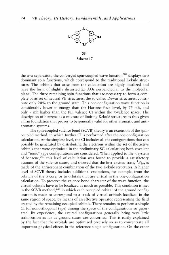
the s–p separation, the converged spin-coupled wave function207 displays twodominant spin functions, which correspond to the traditional Kekule struc-tures. The orbitals that arise from the calculation are highly localized andhave the form of slightly distorted 2p AOs perpendicular to the molecularplane. The three remaining spin functions that are necessary to form a com-plete basis set of neutral VB structures, the so-called Dewar structures, contri-bute only 20% to the ground state. This one-configuration wave function isconsiderably lower in energy than the Hartree–Fock level, by 75 mh, andonly 7 mh higher than the full valence CI within the p-valence space. Thedescription of benzene as a mixture of limiting Kekule structures is thus givena firm foundation that proves to be generally valid for other aromatic and anti-aromatic systems.

The spin-coupled valence bond (SCVB) theory is an extension of the spin-coupled method, in which further CI is performed after the one-configurationcalculation. At the simplest level, the CI includes all the configurations that canpossibly be generated by distributing the electrons within the set of the activeorbitals that were optimized in the preliminary SC calculation; both covalentand ‘‘ionic’’ type configurations are considered. When applied to the p systemof benzene,207 this level of calculation was found to provide a satisfactoryaccount of the valence states, and showed that the first excited state, 1B2u, ismade of the antiresonant combination of the two Kekule structures. A higherlevel of SCVB theory includes additional excitations, for example, from theorbitals of the s core, or to orbitals that are virtual in the one-configurationcalculation. To preserve the valence bond character of the wave function, thevirtual orbitals have to be localized as much as possible. This condition is metin the SCVB method,223 in which each occupied orbital of the ground config-uration is made to correspond to a stack of virtual orbitals localized in thesame region of space, by means of an effective operator representing the fieldcreated by the remaining occupied orbitals. There remains to perform a simpleCI (of nonorthogonal type) among the space of the configurations so gener-ated. By experience, the excited configurations generally bring very littlestabilization as far as ground states are concerned. This is easily explainedby the fact that the orbitals are optimized precisely so as to concentrate allimportant physical effects in the reference single configuration. On the other

Scheme 17


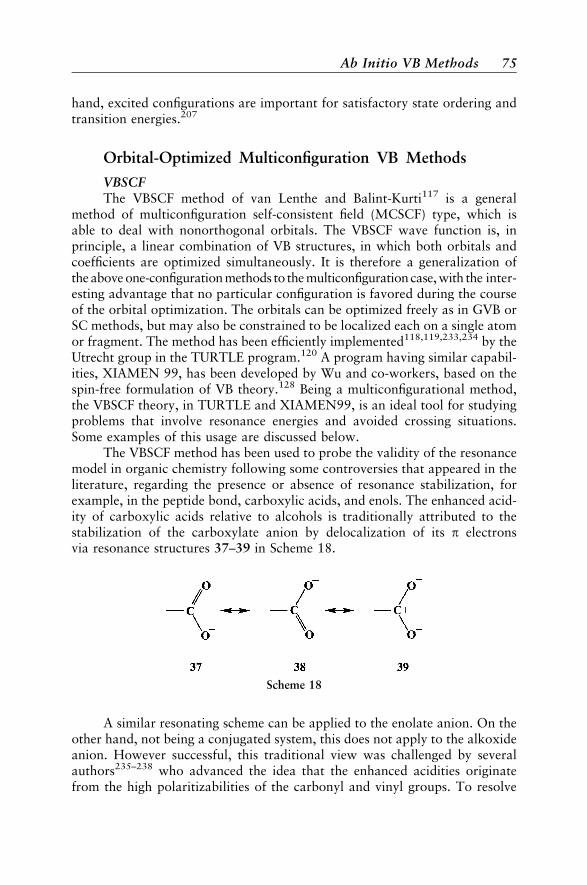
hand, excited configurations are important for satisfactory state ordering andtransition energies.207

Orbital-Optimized Multiconfiguration VB Methods

VBSCFThe VBSCF method of van Lenthe and Balint-Kurti117 is a general

method of multiconfiguration self-consistent field (MCSCF) type, which isable to deal with nonorthogonal orbitals. The VBSCF wave function is, inprinciple, a linear combination of VB structures, in which both orbitals andcoefficients are optimized simultaneously. It is therefore a generalization ofthe above one-configuration methods to the multiconfiguration case,with the inter-esting advantage that no particular configuration is favored during the courseof the orbital optimization. The orbitals can be optimized freely as in GVB orSC methods, but may also be constrained to be localized each on a single atomor fragment. The method has been efficiently implemented118,119,233,234 by theUtrecht group in the TURTLE program.120 A program having similar capabil-ities, XIAMEN 99, has been developed by Wu and co-workers, based on thespin-free formulation of VB theory.128 Being a multiconfigurational method,the VBSCF theory, in TURTLE and XIAMEN99, is an ideal tool for studyingproblems that involve resonance energies and avoided crossing situations.Some examples of this usage are discussed below.

The VBSCF method has been used to probe the validity of the resonancemodel in organic chemistry following some controversies that appeared in theliterature, regarding the presence or absence of resonance stabilization, forexample, in the peptide bond, carboxylic acids, and enols. The enhanced acid-ity of carboxylic acids relative to alcohols is traditionally attributed to thestabilization of the carboxylate anion by delocalization of its p electronsvia resonance structures 37–39 in Scheme 18.

A similar resonating scheme can be applied to the enolate anion. On theother hand, not being a conjugated system, this does not apply to the alkoxideanion. However successful, this traditional view was challenged by severalauthors235–238 who advanced the idea that the enhanced acidities originatefrom the high polaritizabilities of the carbonyl and vinyl groups. To resolve

Scheme 18


the controversy, one must answer the key question: how much does p electrondelocalization stabilize the carboxylate and enolate anions relative to a refer-ence situation in which the delocalization would be ‘‘turned off’’? Clearly, ameaningful answer to this question would emerge only when the orbitals inthe VB wave function are strictly localized, as in the VBSCF method.

A direct estimate of the stabilization energy due to delocalization is verysimple, as illustrated with the following example of the carboxylate anion, inScheme 18. First, a localized reference state is calculated, in which the geome-try and the orbitals are optimized with the unique restriction that the p atomicorbital of one of the oxygens cannot delocalize over the other atoms andremains doubly occupied, as in 37. Second, the ground state is calculated atthe same level of theory, but with electron delocalization being fully allowed.The results of the calculations239 give a clear-cut answer: In all cases the delo-calization of the oxygen p lone pair stabilizes the anion more than the parentacids. These excess values are 23 kcal/mol for carboxylic acids and 21 kcal/mol for enols compared with only 8 kcal/mol for alcohols. It follows that,in accord with the traditional view, p electron delocalization plays an impor-tant role in the acidity enhancement of carboxylic acids and enols relative toalcohols. By comparison with the experimental acidities, it was concluded239

that a lower limit for the contribution of electron delocalization to the totalacidity enhancement is 48% for the carboxylic acids and 62% for the enols,values that clearly establish the importance of resonance effects, while leavingsome room for nonnegligible inductive effects.

The peptide and thio-peptide bonds have some specific properties likecoplanarity, substantial rotational barrier and kinetic stability towards nucleo-philic attack or hydrolysis. All these properties are easily rationalized by the

classical resonance hybrid model, illustrated in Scheme 19 for an amide.According to this resonating picture, the peptide bond is mainly describedby 40, with a significant contribution from the charge-transfer structure 41,and this resonance contribution is the root cause of both the low basicity ofthe nitrogen’s lone pair and the barrier to rotation around the CN bond.

As in the preceding case, the simple resonance picture was critic-ized240–242 on the basis of electron population analyses using the AIM meth-od,243 to the extent that (thio)amides were proposed to be viewed as special

Scheme 19


cases of amines with a carbonyl substituent.242 At the heart of the debate244–

247 was the role of thep electron delocalization energy in the barrier to rotation (16kcal/mol for formamide, 18 kcal/mol for thioformamide248) around the CNbond. To settle the question, the adiabatic energy difference between the loca-lized form 40, with the p lone pair localized on the nitrogen atom, and thefully delocalized ground state, was calculated249 for formamide and thiofor-mamide with the VBSCF method,117 and the same type of calculation wasrepeated for the 90� rotated conformations. As a result, the contribution ofresonance stabilization to the rotational barrier, estimated as that quantityby which electron delocalization stabilizes the planar conformation morethan the 90� rotated conformation, was found to be 7.3 and 13.7 kcal/mol,respectively, for formamide and thioamide. While this indicates that other fac-tors do contribute to the rotational barrier, resonance stabilization in amidesand thioamides emerges as an important factor, in agreement with the tradi-tional view and the common wisdom that allylic resonance is an importantdriving force in organic chemistry.

Clearly, therefore, VBSCF constitutes a handy tool for studies of the roleof electronic delocalization, in molecules that possess more than one Lewisstructure.

VBCI: A Post VBSCF Method that Involves Dynamic CorrelationThe VBCI method, recently developed by Wu et al.138 is a post-VBSCF

calculation that uses configuration interaction to supplement the VBSCFenergy with dynamic correlation. At the same time, the method preservesthe interpretability of the final wave function in terms of a minimal numberof VB structures, each having a clear chemical meaning. The VB structuresthat are used in the VBSCF calculations are referred to as fundamental struc-tures, denoted as �0

K, and the orbitals that appear in the VBSCF calculationare referred to as occupied orbitals. Depending on the problem at hand, theVBSCF calculation may use semidelocalized CF orbitals, or orbitals that areeach localized on a single atom or fragment; in the latter case the fundamentalstructures will explicitly involve the covalent and ionic components of the bonds.

The CI calculation that follows the VBSCF step requires the definition ofvirtual orbitals. To keep the interpretability of the final wave function, the vir-tual orbitals are defined, by use of a projector, so as to be localized on the samefragments as the corresponding occupied orbitals. After generating the virtualorbitals, the excited VB structures are created in the following way. Given afundamental structure �0

K, an excited VB structure �iK is built-up by replacing

occupied orbital(s) ji with virtual orbital(s) j�j . By restricting the replacementof virtual orbital j�j to the same fragment as ji, the excited structure �i

K

retains the same electronic pairing pattern and charge distribution as �0K. In

other words, both �0K and �i

K describe the same classical VB structure.Thus, the collection of excited VB structures nascent from a given fundamentalVB structure serves to relax the latter and endow it with dynamic correlation.


Several levels of CI can be employed. The starting point always involvessingle excitations and is referred to as VBCIS. This can be followed byVBCISD, VBCISDT, and so on, where D stands for double excitations andT for triples. The level at which truncation is made will depend on the sizeof the problem and the desired accuracy. In practice, the VBCISD level hasbeen tested for some dissociation energies and reaction barriers for hydrogenexchange reactions138,142 and has been shown to match the accuracy of themolecular orbital based coupled cluster CCSD and CCSD(T) methods, whileretaining the interpretability of simpler VB methods. In the case of the hydro-gen exchange reaction142 of HþH2, the method gave a barrier of 10 kcal/mol,compatible with the corresponding experimental data (9.6–9.8 kcal /mol). Insummary: The VBCI method can be used like the VBSCF method for problemsinvolving resonance and for calculating VBSCDs. The accuracy of VBCI iscomparable to CCSD and CCSD(T) methods.

Different Orbitals for Different VB StructuresThere are many molecules, in particular some radicals, that are naturally

described in terms of two or more resonance structures, and for which the one-configuration approximation is not appropriate. Such molecules are generallysubject to the well-known broken-symmetry artifact, whereby a wave functioncalculated at an insufficient level of theory is of lower symmetry than thenuclear framework, which results in erroneous energetics and discontinuitiesof the calculated potential surface. The formyloxyl radical (42 $ 43 inScheme 20) is a typical example, but the problem is very general and includes

an enormous variety of open-shell electronic states, as, for example, allyl radi-cals250 or radicals of allylic type,251–256 core-ionized diatoms,257 n–p� excitedmolecules containing two equivalent carbonyl groups,258 n-ionized moleculeshaving equivalent remote lone pairs,259 and charged clusters.260–263 The same pro-blem arises in localized versus mixed-valent organometallic species with twometal ions that can have different oxidation states, in doped stacks of aromaticconductors and semiconductors, and in electron-transfer processes betweentwo identical species (e.g., metal ion centers separated by a bridge). Clearly,this is a ubiquitous problem in chemistry.

Scheme 20


The problem has been lucidly rationalized by McLean et al.255 in VBterms. It arises from a competition between two VB-related effects. The firstis the familiar resonance effect whereby a mixture of two resonance structuresis lower in energy than either one taken separately. The other is the so-calledorbital size effect, whereby each VB structure gains stabilization if it can haveits particular set of orbitals, which are specifically optimized for that VB struc-ture and not the other. The two effects cannot be taken into account simulta-neously in any one-configuration theory, be it of VB or MO type, because itemploys a common set of orbitals. In the (frequent) case where the orbital sizeeffect is the important factor, the wave function takes more or less the form ofone particular VB structure, thereby resulting in an artefactual symmetry-breaking. In the MO-based framework, the remedy consists of performingMCSCF calculations in a rather large space of configurations.255 On the otherhand, the remedy is very simple in the VB framework, and consists of allowingdifferent orbitals for different VB structures in the course of the orbital opti-mization, as illustrated in Scheme 21, by 44 and 45 for the formyloxyl radical,

in which the doubly occupied orbitals are diffuse and hence drawn larger thanthe more compact singly occupied ones. Note that all the orbitals of 44 aredifferent from those of 45, although the major differences are seen betweenthe two orbitals that are involved in the electron transfer.

In the spirit of the above described method, Jackels and Davidson252

cured the symmetry-breaking problem in the NO2 radical by using a sym-metry-adapted combination of two symmetry-broken Hartree–Fock wavefunctions, by means of a 2� 2 nonorthogonal CI. The generalized multistruc-tural (GMS) method of Hollauer and Nascimento264,265 includes both thesymmetry broken structures and the symmetry-adapted one in the same calcu-lation, followed by subsequent CI. The symmetry-broken subwave functionsare optimized at the GVB level in the R-GVB (Resonating-GVB) method ofVoter and Goddard.257 In all these methods, the subwave functions represent-ing the individual resonance structures are optimized separately, which maylead to an underestimation of the resonance energy since the orbital optimiza-tion only takes care of the size effect. To remedy this defect, Voter and God-dard subsequently improved their method by allowing the subwave functions

Scheme 21


to be optimized in the presence of each other, leading to the final generalizedresonating valence bond method (GRVB).258

Breathing Orbitals: A Post VBSCF Method that InvolvesDynamic CorrelationThe breathing orbital valence bond (BOVB) method132–137 is a general-

ization of the principle of ‘‘different orbitals for different structures’’ to thedescription of the elementary bond, be it of the one-electron, two-electron,or three-electron type. The objective of the method is threefold: (a) yieldingaccurate bond dissociation energy curves, which is a necessary conditionfor a meaningful description of the elementary events of a reaction, bondbreaking and bond formation; (2) keeping the wave function compact andtransparent in terms of structural formulas; (3) being suitable for calculationsof diabatic states. In order to achieve these requirements, the method rests onthe basic principle that if all relevant structural formulas for a given electronicsystem are generated, and if their VB description is made optimal by a properorbital optimization, then a variational combination of the corresponding VBstructures would accurately reproduce the energetics of this electronic systemthroughout a reaction coordinate. Accordingly, the composite VB structures ofCF type are abandoned and the wave function takes a classical VB form inwhich all possible structural formulas (e.g., covalent and ionic) are generated.Then, each structural formula is made to correspond to a single VB structurethat displays the appropriate orbital occupancy.

Since the ionic and covalent components of the bonds are explicitlyincluded in the wave function, it is not necessary (and in fact, not useful) tolet the orbitals of the VB structures be delocalized. This exclusion permits abetter interpretability of the wave function in terms of unambiguous structuralformulas, by dealing with VB structures defined with orbitals that are eachstrictly localized on a single atom or fragment. Within this constraint, the orbi-tals are optimized with the freedom to be different for different VB structures,so as to minimize the energy of the full multistructure wave function. It isimportant to note that the different VB structures are not optimized separatelybut in the presence of each other, so that the orbital optimization not only low-ers the energies of each individual VB structure but also maximizes the reso-nance energy resulting from their mixing. As such, the BOVB wave function isa post-VBSCF method that incorporates dynamic correlation.

The difference between the BOVB and GVB or SC philosophies is bestappreciated by comparing their respective descriptions of the two-electronbond. The classical representation for the GVB or SC wave function, obtainedafter expansion of the CF expression into AO determinants as in Eq. [7], takesthe form of a linear combination of covalent and ionic classical VB structures(46–48), for which both coefficients and orbitals are optimized. However,there is the penalizing restriction that the same common set of AOs is usedfor all three structures, as shown in Scheme 22 for the F2 molecule.


On the other hand, the BOVB method assumes the three-structure clas-sical form of the wave function right at the outset. Like the GVB or SC meth-ods, it optimizes the coefficients and the orbitals simultaneously, but with theimportant feature that each VB structure (49–51) may now have its specific setof orbitals, different from one structure to the other, as pictorially representedin Scheme 23, for the same FF bond.

As a consequence of the BOVB procedure, the active orbitals (thoseinvolved in the bond) can use this extra degree of freedom to adapt themselvesto their instantaneous occupancies. The spectator orbitals (not involved in thebond) can fit the instantaneous charges of the atoms to which they belong.Thus, all the orbitals follow the charge fluctuation that is inherent to anybond by undergoing instantaneous changes in size and shape, hence thename ‘‘breathing orbitals’’. The same philosophy underlies the descriptionof odd-electron bonds, in terms of two VB structures.

Since the BOVB wave function takes a classical VB form, it is not prac-tical for the VB description of large electronic systems, because a large numberof VB structures would have to be generated in such a case. As such, the usualway of applying BOVB is to describe with it only those orbitals and electronsthat undergo significant changes in the reaction, like bond breaking or forma-tion, while the remaining orbitals and electrons are described as doubly occu-pied MOs. Thus, even though the spectator electrons reside in doublyoccupied MOs, these orbitals too are allowed to optimize freely, but are other-wise left uncorrelated.

Scheme 22

Scheme 23


The BOVB method has several levels of accuracy. At the most basic level,referred to as L-BOVB, all orbitals are strictly localized on their respectivefragments. One way of improving the energetics by allowing more degreesof freedom is to let the inactive orbitals get delocalized. This option, whichdoes not alter the interpretability of the wave function, accounts better forthe nonbonding interactions between the fragments and is referred to as D-BOVB. Another improvement can be achieved by incorporating radial electroncorrelation in the active orbitals of the ionic structures, by allowing the doublyoccupied orbitals to split into two singly occupied orbitals that are spin-paired.This option carries the label ‘‘S’’ (for split), leading to the SL-BOVB, and SD-BOVB levels of calculation, the latter being the most accurate.

The BOVB method has been successfully tested for its ability to repro-duce dissociation energies and/or dissociation energy curves close to full CIresults or other highly accurate calculations performed with the same basissets. A variety of two-electron and odd-electron bonds, including difficulttest cases as F2, FH, or F2 ,133–135 and the H3MCl series (M¼C, Si, Ge,Sn, Pb)137,155,266 were investigated. Owing to its use of strictly localized activeorbitals, the method is suitable for calculating clearly defined diabatic statesthat are supposed to retain the physical features of a given asymptotic stateat any point of a reaction coordinate without collapsing to the ground stateby virtue of uncontrolled orbital optimization.

It is interesting to interpret the improvement of BOVB with respect to aCASSCF, GVB, or SC calculation of a two-electron bond. These four methodsaccount for all the nondynamic correlation associated with the formation ofthe bond from separate fragments, but differ in their dynamic correlation con-tent. In a medium-sized basis set, say 6-31þG(d), CASSCF, GVB, or SCaccount for less than one-half of the bonding energy of F2, 14–16 kcal/mol.133 On the other hand, an SD-BOVB calculation yields a bonding energyof 36.2 kcal/mol,a versus an experimental value of 38.2 kcal/mol.137 Wheredoes this difference come from? It appears that the BOVB method bringsjust what is missing in the CASSCF calculation, that is, dynamical correlation,not all of it but just that part that is associated to the bond that is being brokenor formed. In other words, the BOVB method takes care of the differentialdynamical correlation. In this respect it is approximately equivalent to theVBCI method.

The importance and physical nature of dynamic correlation is even betterappreciated in the case of three-electron bonds, a type of bond in which theelectron correlation is entirely dynamic, since there is no left–right correlation

aNote that this bonding energy is overestimated with respect to a full CI calculation for the

same basis set, which is estimated as close to 30 kcal/mol. The SD-BOVB systematically

overestimates bonding energies relative to full CI and yields values that are intermediate between

full CI and experiment, a ‘‘fortunate’’ systematic error that compensates for basis set insufficiency.


associated with odd-electron bonds. As has been noted above, the Hartree–Fock and simple VB functions for three-electron bonds (hence GVB, SC, orVBSCF) are nearly equivalent and yield similar bonding energies. If we takethe F2 radical anion as an example, it turns out that the Hartree–Fock bondingenergy is exceedingly poor, only 4 kcal/mol at the spin-unrestricted Hartree–Fock level (UHF), and even worse at the restricted Hartree–Fock (RHF) level,while the experimental bonding energy is 30.3 kcal/mol. By contrast, the SD-BOVB calculation, which involves only two VB structures (52, 53) withbreathing orbitals as in Scheme 24 below, yields an excellent bonding energyof 28.0 kcal/mol.

Looking at 52 and 53 in Scheme 24 allows a clear understanding of thenature of the dynamic correlation effect. Indeed, with respect to a Hartree–Fock or VBSCF calculation, the BOVB wave function brings the additionaleffect that the orbitals adapt themselves to the net charge of each fragment,for example, being more diffuse when the fragment is negatively chargedand less so when the fragment is neutral. This effect, which we have calledthe ‘‘breathing orbital effect’’ but which is called ‘‘size effect’’ by others, cor-responds to the differential dynamic correlation associated with the bond, andis just the instantaneous adaptation of the orbitals to the dynamic charge fluc-tuations that transpire in the bond. This interpretation of dynamic correlation,which is particularly apparent in the three-electron bond, carries over to thetwo-electron bond (e.g., F2 above) that also undergoes some charge fluctuationthrough its ionic components.

The BOVB method has been used for many applications relevantto bonding in organic, inorganic, and organometallic chemis-try.133,134,155,167,168,266–274 Recently, the L-BOVB method was applied tocompute the barriers to hydrogen abstraction in the series X� þHX’! XHþ �X’, and gave results comparable with CCSD at the same basisset.167

In summary, the VBSCF,117–120 VBCI,138 and BOVB133–137 methods areideal tools for studying bonding and for generating VBSCDs for chemical reac-tions. However, while VBSCF will provide a qualitatively correct picture, bothVBCI and BOVB methods will give quantitatively good results in addition to alucid chemical picture.

Scheme 24


PROSPECTIVE

The many examples included in this chapter clearly demonstrate that farfrom being dead, VB theory is a vibrant field of research that produces manynew methods and key paradigms of chemical bonding and reactivity. It ishoped that this chapter will serve its intended purpose of teaching some ele-ments of this theory.

This review of VB theory and its applications is by no means exhaustive.The two most important omissions are the applications of this theory to thestudy of chemical dynamics and to enzymatic chemistry. Ever since the pio-neering paper of London on the potential energy surface of H3,275 and thepaper of Eyring and Polanyi276 on elementary reactions, most of the surfacesused in the studies of chemical dynamics are based on VB formalisms andthinking, for example, LEPS surfaces, and those generated by application ofDIM theory or the BEBO methods.277,278 This kind of thinking was recentlyextended to the treatment of large molecules in the molecular mechanics-basedVB method, called MCMM.140,173 The empirical VB (EVB) method, initiatedby Warshel and Weiss,99 has gradually evolved into a general QM(EVB)/MMmethod100,101 for the study of enzymatic reactions within their native proteinenvironment. Owing to its lucid insight into chemical reactivity the prospectsof this VB-based method are far reaching, and an example is a recent analysisof the role of near-attack-configuration (NAC) in enzymatic catalysis.279 Else-where, in the field of enzymatic reactions, the use of VB ideas led to new para-digms, such as the notion of a chameleon oxidant, for the active species of theenzyme cytochrome P450.280 Thus, in many respects, VB theory is coming ofage, with the development of faster, and more accurate ab initio VB meth-ods,142 and with generation of new post-Pauling concepts. As these activitiesflourish further, so will the usage of VB theory spread among practicingchemists.

APPENDIX

A.1 Expansion of MO Determinants in Terms of AODeterminants

Let DMO be a single determinant involving molecular spin orbitals ji andjj, which can be of a or b spins:

DMO ¼ j � � �ji � � �jJ � � � j ½A1�

ji ¼Xm

Cmiwm ½A2�

jj ¼Xn

Cnj wn ½A3�


Replacing ji and jj in Eq. [A1] by their expansions in terms of AOs,DMO can be expanded into a linear combination of AO-based determinants.The procedure is carried out in the same manner by which one would expand asimple product of orbitals, as long as one remembers that the ordering of theorbitals is important in the AO determinants, and that two determinants thatdiffer by permutation of two of their orbitals are equivalent but of oppositesign. Thus, many AO determinants in Eq. [A4] can be regrouped after permut-ing their orbitals and changing their signs.

j � � �ji � � �jj � � � j ¼Xm

Cmiwm

!� � �

Xn

Cnj wn

!��

¼Xm

Cmi � � �Xn

Cnj � � � j � � � wm � � � wn � � � j ½A4�

While this is a trivial matter for small determinants, larger ones require a bit ofalgebra and a systematic method74 that is shown below.

Let us consider the determinant DMO below as being composed of two‘‘half-determinants’’, ha

MO and hbMO, one regrouping the spin-orbitals of a spins

and the other those of b spins.

DMO ¼ ðhaMO; h

bMOÞ ½A5�

Half-determinants have no physical meaning but are defined here as a conve-nient mathematical intermediary. Each of these MO-based half-determinantscan be expanded into AO-based half-determinants, just as has been done forthe determinants in Eq. [A4]. After orbital permutations the AO-based half-determinants that are equivalent are regrouped, and we are left with someAO-based half-determinants ha

r , each having a unique collection of AOs

haMO ¼

Xr

Car ha

r ½A6�

where the label r designates a given set of AOs.The coefficients of each of these AO half-determinants in the expansion

is given by Eq. [A7]:

Car ¼

XP

ð1ÞtPð� � � � Cmi � � � � � Cnj � � �Þ ½A7�

where P is a permutation between indices m and n and t is the parity of thepermutation. By associating two AO half-determinants ha

r and hbs , one gets

the full AO-based determinant ðhar ; h

bs Þ whose coefficient in the expansion of

Appendix 85

DMO is just the product of the coefficients of its two half-determinants:

DMO ¼Xr;s

Car Cb

s ðhar ; h

bs Þ ½A8�

A.2 Guidelines for VB Mixing

Derivation of matrix elements between polyelectronic VB determinantsfollows from the discussion in the text, and can be carried out by enumeratingall the permutations of the respective diagonal terms, as in Eq. [A9]. Subse-quently, one must define the reduced matrix element in Eq. [A10].52

h�jHeffj�0i ¼ �d

XhðiÞ

�� Xð1Þt Pð�0dÞD E

½A9�

h�jHeffj�0ireduced ¼ h�jHeffj�0i 0:5ðEð�Þ þ Eð�0ÞÞh�j�0i ½A10�

Unfortunately, the retention of overlap leads to many energy and overlapterms that need to be collected and organized, making this procedure quitetedious. A practice that we found useful and productive is to focus on the lead-ing term of the matrix element. In this respect, we show a few qualitativeguidelines that were derived in detail in the original paper52 and discussed else-where.53,84,143 Initially, one has to arrange the two VB determinants withmaximum correspondence of their spin–orbitals. Then, one must find the num-ber of spin–orbitals that are different in the two determinants, and apply thefollowing rules.

1. The first and foremost rule is that the entire matrix element between twoVB determinants is signed as the corresponding determinant overlap andhas the same power in AO overlap. For example, the overlap between thetwo determinants of an HL bond, j ab j and j a b j is S2

ab, and hence thematrix element is negatively signed, 2babSab. Since bab is proportional toSab, both the matrix element and the determinant overlap involve AOoverlap to the power 2. For the one-electron bond case (Eq. [51]), theoverlap between the determinants is þSab and the matrix element þbab,while for the three-electron bond situation (Eq. [52]) the overlap betweenthe determinants j aa b j and j bb a j is Sab and the matrix element islikewise bab.

2. When the VB determinants differ by the occupancy of one spin-orbital, sayorbital a in one determinant is replaced by b in the other (keeping theordering of the other orbitals unchanged), the leading term of the matrixelement will be proportional to bab. Both the one- and three-electron bondsare cases that differ by a single electron occupancy and the correspondingmatrix elements are indeed �b, with a sign as the corresponding overlapbetween the determinants.


3. When the VB determinants differ by the occupancy of two spin–orbitals,the leading term of the matrix element will be the sum of the correspondingbijSij terms with the appropriate sign. An example is the matrix element2babSab between the j ab j and j ab j determinants, which differ by theoccupancy of two spin–orbitals, a and b.

4. The above considerations are the same whether the spin–orbitals are AOs,CF orbitals, or FOs.

A.3 Computing Mono-Determinantal VB Wave Functionswith Standard Ab Initio Programs

This technique utilizes a possibility that is offered by most ab initio stan-dard programs to compute the energy of the guess function even if it is made ofnonorthogonal orbitals. The technique orthogonalizes the orbitals withoutchanging the Slater determinant, then computes the expectation energy byuse of Slater’s rules. In the course of the subsequent optimization of theHartree–Fock orbitals, this expectation value of the energy appears as theenergy at iteration zero. If the guess determinant is made of localized bondingorbitals that typify a given VB structure, then the expectation energy of thiswave function at iteration zero defines the energy of this VB structure. Practi-cally, the localized bonding orbitals that are used to construct the guess deter-minant can be determined by any convenient means. For example, a Kekulestructure of benzene will display a set of three two-centered p-bonding MOsthat can arise from the Hartree–Fock calculation of an ethylene mole-cule.196,281 In a VBSCD calculation, the energy of the crossing point will bethe energy of a guess function made of the orbitals of the reactants, but inthe geometry of the transition state, without further orbital optimization.The zero-iteration technique has also been used to estimate the energy ofspin-alternated determinants (quasi-classical state).175,198

ACKNOWLEDGMENTS

The research at Hebrew University is supported in part by a grant (to SS) from the IsraeliScience Foundation. The two authors are thankful to all their co-workers during their years ofcollaboration (1985–present). Joop van Lenthe and Wei Wu are especially thanked for makingtheir programs (TURTLE and XIAMEN99) available to us. Sam de Visser is acknowledged forproofing the chapter.

REFERENCES

1. Valence Bond Theory, D. L. Cooper, Ed., Elsevier, Amsterdam, The Netherlands, 2002.

2. J. W. Servos, Physical Chemistry from Ostwald to Pauling, Princeton University Press,Princeton, New Jersey, 1990.

References 87

3. S. G. Brush, Stud. Hist. Phil. Sci., 30, 21 (1999). Dynamics of Theory Change in Chemistry:Part 1. The Benzene Problem 1865–1945.

4. S. G. Brush, Stud. Hist. Phil. Sci. 30, 263 (1999). Dynamics of Theory Change in Chemistry:Part 2. Benzene and Molecular Orbitals, 1945–1980.

5. G. N. Lewis, J. Am. Chem. Soc., 38, 762 (1916). The Atom and the Molecule.

6. I. Langmuir, J. Am. Chem. Soc., 41, 868 (1919). The Arrangement of Electrons in Atoms andMolecules.

7. W. Heitler and F. London, Z. Phys., 44, 455 (1927). Wechselwirkung Neutraler Atome unHomoopolare Bindung nach der Quantenmechanik.

8. For an English translation, see H. Hettema, Quantum Chemistry Classic Scientific Paper,World Scientific, Singapore, 2000.

9. W. Heisenberg, Z. Phys., 411, 38, (1926). Mehrkorperproblem und Resonanz in derQuantenmechanik,

10. F. London Z. Phys., 455, 46, (1928). On The Quantum Theory of Homo-polar ValenceNumbers.

11. L. Pauling, Proc. Natl. Acad. Sci. U.S.A., 14, 359 (1928). The Shared-Electron ChemicalBond.

12. J. C. Slater, Phys. Rev., 34, 1293 (1929). The Theory of Complex Spectra.

13. J. C. Slater, Phys. Rev., 38, 1109 (1931). Molecular Energy Levels and Valence Bonds.

14. G. Rumer, Gottinger Nachr., 27, 337 (1932). Zum Theorie der Spinvalenz.

15. G. A. Gallup, in Valence Bond Theory, D. L. Cooper, Ed., Elsevier, Amsterdam, TheNetherlands, 2002, pp. 1–40. A Short History of VB Theory.

16. J. C. Slater, Phys. Rev., 37, 481 (1931). Directed Valence in Polyatomic Molecules.

17. J. C. Slater, Phys. Rev., 41, 255 (1931). Note on Molecular Structure.

18. L. Pauling, J. Am. Chem. Soc., 53, 1367 (1931). The Nature of the Chemical Bond.Application of Results Obtained from the Quantum Mechanics and from a Theory ofMagnetic Susceptiblity to the Structure of Molecules.

19. L. Pauling, J. Am. Chem. Soc., 53, 3225 (1931). The Nature of the Chemical Bond. II. TheOne-Electron Bond and the Three-Electron Bond.

20. L. Pauling, The Nature of the Chemical Bond, Cornell University Press, Ithaca, New York,1939 (3rd ed., 1960).

21. R. S. Mulliken, Phys. Rev., 32, 186 (1928). The Assignment of Quantum Numbers forElectrons in Molecules. I.

22. R. S. Mulliken, Phys. Rev., 32, 761 (1928). The Assignment of Quantum Numbers forElectrons in Molecules. II. Correlation of Atomic and Molecular Electron States.

23. R. S. Mulliken, Phys. Rev., 33, 730 (1929). The Assignment of Quantum Numbers forElectrons in Molecules. III. Diatomic Hydrides.

24. R. S. Mulliken, Phys. Rev., 41, 49 (1932). Electronic Structures of Polyatomic Molecules andValence. II. General Considerations.

25. F. Hund, Z. Phys., 73, 1 (1931). Zur Frage der Chemischen Bindung.

26. F. Hund, Z. Phys., 51, 759 (1928). Zur Deutung der Molekelspektren. IV.

27. J. E. Lennard-Jones, Trans. Faraday Soc., 25, 668 (1929). The Electronic Structure of someDiatomic Molecules.

28. J. A. Berson, Chemical Creativity. Ideas from the Work of Woodward, Huckel, Meerwein, andOthers, Wiley-VCH, NewYork, 1999.

29. E. Huckel, Z. Phys., 60, 423 (1930). Zur Quantentheorie der Doppelbindung.

30. E. Huckel, Z. Phys., 70, 204 (1931). Quantentheoretische Beitrag zum Benzolproblem. I. DiesElektronenkonfiguration des Benzols und verwandter Verbindungen.


31. E. Huckel, Z. Phys., 76, 628 (1932). Quantentheoretische Beitrag zum Problem der Aroma-tischen Ungesattigten Verbindungen. III.

32. L. Pauling and G. W. Wheland, J. Chem. Phys., 1, 362 (1933). The Nature of the ChemicalBond. V. The Quantum-Mechanical Calculation of the Resonance Energy of Benzene andNaphthalene and the Hydrocarbon Free Radicals.

33. G. W. Wheland, Resonance in Organic Chemistry, Wiley, New York, 1955, pp. 4, 39, 148.

34. J. H. van Vleck and A. Sherman, Rev. Mod. Phys., 7, 167 (1935). The Quantum Theory ofValence.

35. P. Laszlo and R. Hoffmann, Angew. Chem. Int. Ed., 39, 123 (2000). Ferrocene: IroncladHistory or Roshomon Tale?

36. G. W. Wheland, Proc. R. Soc. London, A159, 397 (1938). The Electronic Structure of SomePolyenes and Aromatic Molecules. V—A Comparison of Molecular Orbital and ValenceBond Methods.

37. G. W. Wheland, J. Chem. Phys., 2, 474 (1934). The Quantum Mechanics of Unsaturated andAromatic Molecules: A Comparison of Two Methods of Treatment.

38. D. P. Craig, J. Chem. Soc., 3175 (1951). Cyclobutadiene and Some Other PseudoaromaticCompounds.

39. D. P. Craig, Proc. R. Soc. London, A200, 498 (1950). Electronic Levels in Simple ConjugatedSystems. I. Configuration Interaction in Cyclobutadiene.

40. C. A. Coulson, Proc. R. Soc. London, A207, 63 (1951). Critical Survey of the Method of Ionic-Homopolar Resonance.

41. M. J. S. Dewar, Electronic Theory of Organic Chemistry, Clarendon Press, Oxford, 1949,pp. 15–17.

42. C. A. Coulson, Valence, Oxford University Press, London, 1952.

43. J. R. Platt, Science, 154, 745 (1966). Nobel Laureate in Chemistry: Robert S. Mulliken.

44. K. Fukui, T. Yonezawa, and H. Shingu, J. Chem. Phys., 20, 722 (1952). A Molecular OrbitalTheory of Reactivity in Aromatic Hydrocarbons.

45. R. B. Woodward and R. Hoffmann, The Conservation of Orbital Symmetry, Verlag Chemie,Weinheim, 1971.

46. M. G. Evans, Trans. Faraday Soc., 35, 824 (1939). The Activation Energies in ReactionsInvolving Conjugated Systems.

47. E. Heilbronner and H. Bock, The HMO Model and its Applications, Wiley, New York, 1976.

48. E. Honegger and E. Heilbronner, in Theoretical Models of Chemical Bonding, Z. B. Maksic,Ed., Springer-Verlag, Berlin- Heidelberg, 1991, Vol. 3, pp. 100–151. The Equivalent OrbitalModel and the Interpretation of PE Spectra.

49. S. Wolfe and Z. Shi, Isr. J. Chem., 40, 343 (2000). The SCO (OCS) Edward-LemieuxEffect is Controlled by p-Orbital on Oxygen. Evidence from Electron Momentum Spectro-scopy, Photoelectron Spectroscopy, X-Ray Crystallography, and Density Functional Theory.

50. P. Atkins and L. Jones, Chemical Principles. The Quest for Insight, W. H. Freeman and Co.,New York, 1999, pp. xxiii and 121–122.

51. L. Jones and P. Atkins, Chemistry Molecules, Matter and Change, W. H. Freeman and Co.,New York, 2000, pp. 400–401.

52. S. Shaik, in New Theoretical Concepts for Understanding Organic Reactions, J. Bertran and I.G. Csizmadia, Eds., NATO ASI Series, C267, Kluwer Academic Publ., 1989, pp. 165–217. AQualitative Valence Bond Model for Organic Reactions.

53. S. Shaik and P. C. Hiberty, Adv. Quant. Chem., 26, 100 (1995). Valence Bond Mixing andCurve Crossing Diagrams in Chemical Reactivity and Bonding.

54. P. C. Hiberty, J. Mol. Struct. (THEOCHEM), 398, 35 (1997). Thinking and ComputingValence Bond in Organic Chemistry.

References 89

55. A. Shurki, F. Dijkstra, P. C. Hiberty, and S. Shaik, J. Phys. Org. Chem., 16, 731 (2003).Aromaticity and Antiaromaticity: What Role Do Ionic Configurations Play in Delocalizationand Induction of Magnetic Properties?

56. W. Heitler and G. Poschl, Nature (London), 133, 833 (1934). Ground State of C2 and O2 andthe Theory of Valency.

57. S. Shaik, A. Shurki, D. Danovich, and P. C. Hiberty, Chem. Rev., 101, 1501 (2001). ADifferent Story of p-Delocalization—The Distortivity of the p-Electrons and Its ChemicalManifestations.

58. A. F. Voter and W. A. Goddard, III, J. Am. Chem. Soc., 108, 2830 (1986). The GeneralizedResonating Valence Bond Description of Cyclobutadiene.

59. J. H. van Vleck, J. Chem. Phys., 3, 803 (1935). The Group Relation Between the Mulliken andSlater–Pauling Theories.

60. H. Zuilhof, J. P. Dinnocenzo, A. C. Reddy, and S. Shaik, J. Phys. Chem., 100, 15774 (1996). AComparative Study of Ethane and Propane Cation Radicals by B3LYP Density Functionaland High-Level Ab Initio Methods.

61. S. Shaik and P. C. Hiberty, Helv. Chem. Acta, 86, 1063 (2003). Myth and Reality in theAttitude Toward Valence-Bond (VB) Theory: Are Its ‘Failures’ Real?’’

62. D. J. Klein, in Valence Bond Theory, D. L. Cooper, Ed., Elsevier, Amsterdam, The Nether-lands, 2002, pp. 447–502. Resonating Valence Bond Theories for Carbon p-Networks andClassical/Quantum Connections.

63. T. G. Schmalz, in Valence Bond Theory, D. L. Cooper, Ed., Elsevier, Amsterdam, TheNetherlands, 2002, pp. 535–564. A Valence Bond View of Fullerenes.

64. J. P. Malrieu, in Theoretical Models of Chemical Bonding, Z. B. Maksic, Ed., Springer-Verlag,Berlin-Heidelberg, 1990, Vol. 1, pp. 108–136. The Magnetic Description of ConjugatedHydrocarbons.

65. J. P. Malrieu and D. Maynau, J. Am. Chem. Soc., 104, 3021 (1984). A Valence Bond EffectiveHamiltonian for Neutral States of p-Systems. 1. Methods.

66. Y. Jiang and S. Li, in Valence Bond Theory, D. L. Cooper, Ed., Elsevier, The Netherlands,Amsterdam, 2002, 565–602. Valence Bond Calculations and Theoretical Applications toMedium-Sized Conjugated Hydrocarbons.

67. F. A. Matsen, Acc. Chem. Res., 11, 387 (1978). Correlation of Molecular Orbital and ValenceBond States in p Systems.

68. M. A. Fox and F. A. Matsen, J. Chem. Educ., 62, 477 (1985). Electronic Structure in p-Systems. Part II. The Unification of Huckel and Valence Bond Theories.

69. M. A. Fox and F. A. Matsen, J. Chem. Educ., 62, 551 (1985). Electronic Structure in p-Systems. Part III. Application in Spectroscopy and Chemical Reactivity.

70. S. Ramasesha and Z. G. Soos, in Valence Bond Theory, D. L. Cooper, Ed., Elsevier,Amsterdam, The Netherlands, 2002, pp. 635–697. Valence Bond Theory of Quantum CellModels.

71. W. Wu, S. J. Zhong, and S. Shaik, Chem. Phys. Lett., 292, 7 (1998). VBDFT(s): A Huckel-Type Semi-empirical Valence Bond Method Scaled to Density Functional Energies. Applica-tions to Linear Polyene.

72. W. Wu, D. Danovich, A. Shurki, and S. Shaik, J. Phys. Chem., A 104, 8744 (2000). UsingValence Bond Theory to Understand Electronic Excited States. Applications to the HiddenExcited State (21Ag) of Polyenes.

73. W. Wu, Y. Luo, L. Song, and S. Shaik, Phys. Chem. Chem. Phys., 3, 5459 (2001). VBDFT(s):A Semiempirical Valence Bond Method: Application to Linear Polyenes Containing Oxygenand Nitrogen Heteroatoms.

74. P. C. Hiberty and C. Leforestier, J. Am. Chem. Soc., 100, 2012 (1978). Expansion of Molecu-lar Orbital Wave Functions into Valence Bond Wave Functions. A Simplified Procedure.

75. T. Thorsteinsson, D. L. Cooper, J. Gerratt, and M. Raimondi, Molecular Engineering, 7, 67(1997). A New Approach to Valence Bond Calculations CASVB.


76. Thorsteinsson, D. L. Cooper, J. Gerratt, P. Kardakov, and M. Raimondi, Theor. Chim. Acta(Berl.), 93, 343 (1996). Modern Valence Bond Representation of CASSCF Wave Functions.

77. H. Nakano, K. Sorakubo, K. Nakayama, and H. Hirao, in Valence Bond Theory, D. L.Cooper, Ed. Elsevier, The Netherlands, Amsterdam, 2002, pp. 55–77. Complete ActiveSpace Valence Bond (CASVB) Method and its Application in Chemical Reactions.

78. K. Hirao, H. Nakano, and K. Nakayama, J. Chem. Phys., 107, 9966 (1997). A CompleteActive Space Valence Bond Method with Nonorthogonal Orbitals.

79. N. D. Epiotis, J. R. Larson, and H. L. Eaton, Lecture Notes Chem., 29, 1 (1982). UnifiedValence Bond Theory of Electronic Structure.

80. N. D. Epiotis, Deciphering the Chemical Bond. Bonding Across the Periodic Table, VCH,New York, 1996, pp. 1-933.

81. S. S. Shaik, J. Am. Chem. Soc., 103, 3692 (1981). What Happens to Molecules As They React?A Valence Bond Approach to Reactivity.

82. A. Pross and S. S. Shaik, Acc. Chem. Res., 16, 363 (1983). A Qualitative Valence BondApproach to Chemical Reactivity.

83. A. Pross, Theoretical and Physical Principles of Organic Reactivity, J. Wiley, New York,1995, pp. 83–124; 235–290.

84. S. Shaik and P. C. Hiberty, in Theoretical Models of Chemical Bonding, Z.B. Maksic, Ed.,Springer-Verlag, Berlin-Heidelberg, 1991, Vol. 4, pp. 269–322. Curve Crossing Diagrams asGeneral Models for Chemical Structure and Reactivity.

85. S. Shaik and A. Shurki, Angew. Chem. Int. Ed. Engl., 38, 586 (1999). Valence Bond Diagramsand Chemical Reactivity.

86. J. W. Linnett, The Electronic Structure of Molecules. A New Approach, Methuen & Co Ltd,London, 1964, pp. 1–162.

87. R. D. Harcourt, Lecture Notes Chem., 30, 1 (1982). Qualitative Valence-Bond Descriptions ofElectron-Rich Molecules: Pauling ‘‘3-Electron Bonds’’ and ‘‘Increased-Valence’’ Theory.

88. R. D. Harcourt, in Valence Bond Theory, D. L. Cooper, Ed., Elsevier, Amsterdam, TheNetherlands, 2002, pp. 349–378. Valence Bond Structures for Some Molecules with FourSingly-Occupied Active-Space Orbitals: Electronic Structures, Reaction Mechanisms, Metal-lic Orbitals.

89. A. Th. Van der Lugt and L. J. Oosterhoff, J. Am. Chem. Soc., 91, 6042 (1969). SymmetryControl and Photoinduced Reactions.

90. J. J. C. Mulder and L. J. Oosterhoff, Chem. Commun., 305 (1970). Permutation SymmetryControl in Concerted Reactions.

91. J. Michl, Topics Curr. Chem., 46, 1 (1974). Physical Basis of Qualitative MO Arguments inOrganic Photochemistry.

92. W.Gerhartz, R. D. Poshusta, and J. Michl, J. Am. Chem. Soc., 99, 4263 (1977). PotentialEnergy Hypersurfaces for H4. 2. ‘‘Triply Right’’ (C2v) Tetrahedral Geometries. A PossibleRelation to Photochemical ‘‘Cross Bonding’’ Processes.

93. F. Bernardi, M. Olivucci, and M. Robb, Isr. J. Chem., 33, 265 (1993). Modeling Photo-chemical Reactivity of Organic Systems. A New Challenge to Quantum ComputationalChemistry.

94. M. Olivucci, I. N. Ragazos, F. Bernardi, and M. A. Robb, J. Am. Chem. Soc., 115, 3710(1993). A Conical Intersection Mechanism for the Photochemistry of Butadiene. A MC-SCFStudy.

95. M. Olivucci, F. Bernardi, P. Celani, I. Ragazos, and M. A. Robb, J. Am. Chem. Soc., 116, 1077(1994). Excited-State Cis-Trans Isomerization of cis-Hexatriene. A CAS–SCF Computa-tional Study.

96. M. A. Robb, M. Garavelli, M. Olivucci, and F. Bernardi, in Reviews in ComputationalChemistry, K. B. Lipkowitz and D. B. Boyd, Eds., Vol. 15, pp. 87–146, (2000). AComputational Strategy for Organic Photochemistry.

References 91

97. S. Shaik and A. C. Reddy, J. Chem. Soc. Faraday Trans., 90, 1631 (1994). Transition States,Avoided Crossing States and Valence Bond Mixing: Fundamental Reactivity Paradigms.

98. S. Zilberg and Y. Haas, Chem. Eur. J., 5, 1755 (1999). Molecular Photochemistry: A GeneralMethod for Localizing Conical Intersections Using the Phase-Change Rule.

99. A. Warshel and R. M. Weiss, J. Am. Chem. Soc., 102, 6218 (1980). Empirical Valence BondApproach for Comparing Reactions in Solutions and in Enzymes.

100. A. Warshel and S. T. Russell, Quart. Rev. Biophys., 17, 282 (1984). Calculations ofElectrostatic Interactions in Biological Systems and in Solutions.

101. A. Warshel, J. Phys. Chem., 83, 1640 (1979). Calculations of Chemical Processes in Solutions.

102. H. J. Kim and J. T. Hynes, J. Am. Chem. Soc., 114, 10508 (1992). A Theoretical Model forSN1 Ionic Dissociation in Solution. 1. Activation Free Energies and Transition-StateStructure.

103. J. R. Mathias, R. Bianco, and J. T. Hynes, J. Mol. Liq., 61, 81 (1994). On the Activation FreeEnergy of the Cl þ CH3Cl SN2 Reaction in Solution.

104. J. I. Timoneda and J. T. Hynes, J. Phys. Chem., 95, 10431 (1991). Nonequilibrium FreeEnergy Surfaces for Hydrogen-bonded Proton Transfer Compexes in Solution.

105. S. Shaik, J. Am. Chem. Soc., 106, 1227 (1984). Solvent Effect on Reaction Barriers. The SN2Reactions. 1. Application to the Identity Exchange.

106. S. Shaik, J. Org. Chem., 52, 1563 (1987). Nucleophilic Reactivity and Vertical IonizationPotentials in Cation–Anion Recombinations.

107. W. A. Goddard, III, T. H. Dunning, Jr., W. J. Hunt, and P. J. Hay, Acc. Chem. Res., 6, 368(1973). Generalized Valence Bond Description of Bonding in Low-Lying States of Molecules.

108. W. A. Goddard, III, Phys. Rev., 157, 81 (1967). Improved Quantum Theory of Many-ElectronSystems. II. The Basic Method.

109. W. A. Goddard, III, and L. B. Harding, Annu. Rev. Phys. Chem., 29, 363 (1978). TheDescription of Chemical Bonding from Ab-Initio Calculations.

110. W. A. Goddard, III, Int. J. Quant. Chem., IIIS, 593 (1970). The Symmetric Group and the SpinGeneralized SCF Method.

111. C. A. Coulson and I. Fischer, Philos. Mag., 40, 386 (1949). Notes on the Molecular OrbitalTreatment of the Hydrogen Molecule.

112. D. L. Cooper, J. Gerratt, and M. Raimondi, Chem. Rev., 91, 929 (1981). Application of Spin-Coupled Valence Bond Theory.

113. D. L. Cooper, J. P. Gerratt, and M. Raimondi, Adv. Chem. Phys., 69, 319 (1987). ModernValence Bond Theory.

114. M. Sironi, M. Raimondi, R. Martinazzo, and F. A. Gianturco, in Valence Bond Theory, D. L.Cooper, Ed., Elsevier, Amsterdam, The Netherlands, 2002, pp. 261–277. Recent Develop-ments of the SCVB Method.

115. G. G. Balint-Kurti and M. Karplus, J. Chem. Phys., 50, 478 (1969). Multistructure Valence-Bond and Atoms-in-Molecules Calculations for LiF, F2, and F2 .

116. J. H. van Lenthe and G. G. Balint-Kurti, Chem. Phys. Lett., 76, 138 (1980). The Valence-BondSCF (VB SCF) Method. Synopsis of Theory and Test Calculations of the OH Potential EnergyCurve.

117. J. H. van Lenthe and G. G. Balint-Kurti, J. Chem. Phys., 78, 5699 (1983). The Valence-BondSelf-Consistent Field Method (VB–SCF): Theory and Test Calculations.

118. J. Verbeek and J. H. van Lenthe, J. Mol. Struct. (THEOCHEM), 229, 115 (1991). On theEvaluation of Nonorthogonal Matrix Elements.

119. J. Verbeek and J. H. van Lenthe, Int. J. Quant. Chem., XL, 201(1991). The GeneralizedSlater–Condon Rules.

120. J. Verbeek, J. H. Langenberg, C. P. Byrman, F. Dijkstra, and J. H. van Lenthe, TURTLE: AnAb Initio VB/VBSCF Program (1998–2000).


121. J. H. van Lenthe, F. Dijkstra, and W. A. Havenith, in Valence Bond Theory, D. L. Cooper, Ed.,Elsevier, Amsterdam, The Netherlands, 2002, pp. 79–116. TURTLE—A Gradient VBSCFProgram Theory and Studies of Aromaticity.

122. F. A. Matsen, Adv. Quant. Chem., 1, 60 (1964). Spin-Free Quantum Chemistry.

123. F. A. Matsen, J. Phys. Chem., 68, 3282 (1964). Spin-Free Quantum Chemistry. II. Three-Electron Systems.

124. R. McWeeny, Int. J. Quant. Chem., XXXIV, 23 (1988). A Spin Free Form of Valence BondTheory.

125. Q. Zhang, and L. Xiangzhu, J. Mol. Struct. (THEOCHEM), 198, 413 (1989). BondedTableau Method for Many Electron Systems.

126. X. Li and Q. Zhang, Int. J. Quant. Chem., XXXVI, 599 (1989). Bonded Tableau UnitaryGroup Approach to the Many-Electron Correlation Problem.

127. W. Wu, Y. Mo, Z. Cao, and Q. Zhang, in Valence Bond Theory, D. L. Cooper, Ed., Elsevier,Amsterdam, The Netherlands, 2002, pp. 143–186. A Spin Free Approach for Valence BondTheory and Its Application.

128. W. Wu, L. Song, Y. Mo, and Q. Zhang, XIAMEN-99– An Ab Initio Spin-free Valence BondProgram, Xiamen University, Xiamen, China, 1999.

129. J. Li and R. McWeeny, VB2000: An Ab Initio Valence Bond Program Based on ProductFunction Method and the Algebrant Algorithm. 2000.

130. G. A. Gallup, R. L. Vance, J. R. Collins, and J. M. Norbeck, Adv. Quant. Chem., 16, 229(1982). Practical Valence Bond Calculations.

131. G. A. Gallup, The CRUNCH Suite of Atomic and Molecular Structure Programs, [email protected].

132. P. C. Hiberty, J. P. Flament, and E. Noizet, Chem. Phys. Lett., 189, 259 (1992). Compact andAccurate Valence Bond Functions with Different Orbitals for Different Configurations:Application to the Two-Configuration Description of F2.

133. P. C. Hiberty, S. Humbel, C. P. Byrman, and J. H. van Lenthe, J. Chem. Phys., 101, 5969(1994). Compact Valence Bond Functions with Breathing Orbitals: Application to the BondDissociation Energies of F2 and FH.

134. P. C. Hiberty, S. Humbel, and P. Archirel, J. Phys. Chem., 98, 11697 (1994). Nature of theDifferential Electron Correlation in Three-Electron Bond Dissociation. Efficiency of a SimpleTwo-Configuration Valence Bond Method with Breathing Orbitals.

135. P. C. Hiberty, in Modern Electronic Structure Theory and Applications in Organic Chemistry,E. R. Davidson, Ed., World Scientific, River Edge, NJ, 1997, pp. 289–367. The BreathingOrbital Valence Bond Method.

136. P. C. Hiberty and S. Shaik, in Valence Bond Theory, D. L. Cooper, Ed., Elsevier, Amsterdam,The Netherlands, 2002, pp. 187–226. Breathing-Orbital Valence Bond—A Valence BondMethod Incorporating Static and Dynamic Electron Correlation Effects.

137. P. C. Hiberty and S. Shaik, Theor. Chem. Acc., 108, 255 (2002). BOVB—A Modern ValenceBond Method That Includes Dynamic Correlation.

138. W. Wu, L. Song, Z. Cao, Q. Zhang, and S. Shaik, J. Phys. Chem. A, 106, 2721 (2002).Valence Bond Configuration Interaction. A Practical Valence Bond Method IncorporatingDynamic Correlation.

139. J. J. W. McDouall, in Valence Bond Theory, D. L. Cooper, Ed., Elsevier, Amsterdam, TheNetherlands, 2002, pp. 227–260. The Biorthogonal Valence Bond Method.

140. T. Albu, J. C. Corchado, and D. G. Truhlar, J. Phys. Chem. A, 105, 8465 (2001). MolecularMechanics for Chemical Reactions: A Standard Strategy for Using MulticonfigurationMolecular Mechanics for Variational Transition State Theory with Optimized Multidimen-sional Tunneling.

141. T. K. Firman and C. R. Landis, J. Am. Chem. Soc., 123, 1178 (2001). Valence Bond ConceptsApplied to Molecular Mechanics Description of Molecular Shapes. 4. Transition Metalswith p-bonds.

References 93

142. L. Song, W. Wu, P. C. Hiberty, and S. Shaik, Chem. Eur. J., 9, 4540 (2003). An AccurateBarrier for the Hydrogen Exchange Reaction. Is This Theory Coming of Age?

143. S. S. Shaik, E. Duzy, and A. Bartuv, J. Phys. Chem., 94, 6574 (1990). The QuantumMechanical Resonance Energy of Transition States: An Indicator of Transition StateGeometry and Electronic Structure.

144. R. McWeeny, J. Mol. Struct. (THEOCHEM), 229, 29 (1991). On the Nature of the OxygenDouble Bond.

145. R. D. Harcourt, J. Phys. Chem., 96, 7616 (1992). Valence Bond Studies of Oxygen andSuperoxides: A Note on One-electron and Two-electron Transfer Resonances.

146. H. Fischer and J. N. Murrell, Theor. Chim. Acta (Berl.), 1, 463 (1963). The Interpretation ofthe Stability of Aromatic Hydrocarbon Ions by Valence Bond Theory.

147. N. D. Epiotis, Nouv. J. Chim., 8, 421 (1984). How to ‘‘Think’’ at the Level of MO—CI TheoryUsing Huckel MO Information!

148. E. Heilbronner, Tetrahedron Lett., 1923 (1964). Huckel Molecular Orbitals of Mobius-TypeConformation of Annulenes.

149. A. A. Frost and B. Musulin, J. Chem. Phys., 21, 572 (1953). A Mnemonic Device forMolecular Orbital Energies.

150. S. C. Wright, D. L. Cooper, J. Gerratt, and M. Raimondi, J. Phys. Chem., 96, 7943 (1992).Spin-coupled Description of Cyclobutadiene and 2,4-Dimethylenecyclobutane-1,3-diyls:Antipairs.

151. P. B. Karadakov, J. Gerratt, D. L. Cooper, and M. Raimondi, J. Phys. Chem., 99, 10186(1995). The Electronic Structure of Cyclooctatetraene and the Modern Valence BondUnderstanding of Antiaromaticity.

152. A. Shurki, VB Theory as a Tool for Understanding Structure and Reactivity in Chemistry,Ph.D. Dissertation, 1999, Hebrew University, Israel.

153. G. Sini, P. Maıtre, P. C. Hiberty, and S. S. Shaik. J. Mol. Struct. (THEOCHEM), 229, 163(1991). Covalent, Ionic and Resonating Single Bonds.

154. S. Shaik, P. Maıtre, G. Sini, and P. C. Hiberty, J. Am. Chem. Soc., 114, 7861 (1992). TheCharge-Shift Bonding Concept. Electron Pair Bonds with Very Large Resonance Energies.

155. A. Shurki, P. C. Hiberty, and S. Shaik, J. Am. Chem. Soc., 121, 822 (1999). Charge-ShiftBonding in Group IVB Halides: A Valence Bond Study of MH3Cl (M¼C, Si, Ge, Sn, Pb)Molecules.

156. S. P. de Visser, D. Danovich, W. Wu, and S. Shaik, J. Phys. Chem. A, 106, 4961 (2002).Ferromagnetic Bonds: Properties of ‘‘No-pair’’ Bonded High-Spin Lithium Clusters; Nþ1LiN(N ¼ 2–12).

157. D. Danovich and S. Shaik, J. Am. Chem. Soc., 121, 3165 (1999). No-Pair Bonding in the High-Spin 3�þu State of Li2. A Valence Bond Study of its Origins.

158. A. Pross, Acc. Chem. Res., 18, 212 (1985). The Single Electron Shift as a Fundamental Processin Organic Chemistry: The Relationship Between Polar and Electron-transfer Pathways.

159. G. Sini, S. S. Shaik, J.-M. Lefour, G. Ohanessian, and P. C. Hiberty, J. Phys. Chem., 93, 5661(1989). Quantitative Valence Bond Computation of a Curve Crossing Diagram for a ModelSN2 Reaction, H þ CH3H0 ! HCH3 þH0.

160. G. Sini, S. Shaik, and P. C. Hiberty, J. Chem. Soc. Perkin Trans., 2, 1019 (1992). QuantitativeValence Bond Computations of Curve Crossing Diagrams for a Gas Phase Reaction,F þ CH3F! FCH3 þ F.

161. J. Mestres and P. C. Hiberty, New J. Chem., 20, 1213 (1996). Quantitative Valence BondComputations of Curve Crossing Diagrams for a Hydride Transfer Model Reaction:CH4 þ CHþ3 ! CHþ3 þ CH4.

162. G. Sini, G. Ohanessian, P. C. Hiberty, and S. S. Shaik, J. Am. Chem. Soc., 112, 1407 (1990).Why is SiH5 a Stable Intermediate While CH5 is a Transition State ? A Quantitative CurveCrossing Valence Bond Study.


163. G. Sini and P. C. Hiberty, J. Chem. Soc. Chem. Commun., 772 (1989). The Origin of theDifferent Bonding Features in SiH5 and CH5 ; A Valence Bond Curve Crossing Model.

164. P. Maıtre, F. Volatron, P. C. Hiberty, and S. S. Shaik, Inorg. Chem., 29, 3047 (1990).Hypercoordination in SiH5 and SiH5. An Electron-count Dependence.

165. P. R. Benneyworth, G. G. Balint-Kurti, M. J. Davis, and I. H. Williams, J. Phys. Chem., 96,4346 (1992). Ab initio Valence Bond Study of the Origin of Barriers to Hydrogen ExchangeReactions: Application of the Valence Bond Self-Consistent-Field Method to theFþHF! FHþ F Reaction.

166. P. Maıtre, P. C. Hiberty, G. Ohanessian, and S. S. Shaik, J. Phys. Chem., 94, 4089 (1990).Quantitative Computations of Curve Crossing Diagrams for Model Atom Exchange Reac-tion.

167. S. Shaik, W. Wu, K. Dong, L. Song, and P. C. Hiberty, J. Phys. Chem. A, 105, 8226 (2001).Identity Hydrogen Abstraction Reactions, XþHX0 ! XHþX0ðX ¼ X0 ¼ CH3, SiH3,GeH3, SnH3, PbH3): A Valence Bond Modeling.

168. L. Song, W. Wu, K. Dong, P. C. Hiberty, and S. Shaik, J. Phys. Chem. A, 106, 11361 (2002).Valence Bond Modeling of Barriers in the Nonidentity Hydrogen Abstraction Reactions,X0� þHX! X0HþX� ðX0 6¼X CH3, SiH3, GeH3, SnH3, PbH3).

169. S. S. Shaik, Prog. Phys. Org. Chem., 15, 197 (1985). The Collage of SN2 Reactivity Patterns: AState Correlation Diagram Model.

170. S. S. Shaik, H. B. Schlegel, and S. Wolfe, Theoretical Aspects of Physical Organic Chemistry,Wiley-Interscience, New York, 1992.

171. Y. Mo and S. D. Peyerimhoff, J. Chem. Phys., 109, 1687 (1998). Theoretical Analysis ofElectronic Delocalization.

172. F. Jensen and P.-O. Norrby, Theor. Chim. Acc. 109, 1 (2003). Transition States fromEmpirical Force Fields.

173. Y. Kim, J. C. Corchado, J. Villa, J. Xing, and D. G. Truhlar, J. Chem. Phys., 112, 2718 (2000).Multiconfiguration Molecular Mechanics Algorithm for Potential Energy Surfaces of Che-mical Reactions.

174. F. Jensen, Introduction to Computational Chemistry, Wiley, New York, 1999, pp. 48–49.

175. R. Mereau, M. T. Rayez, J. C. Rayez, and P. C. Hiberty, Phys. Chem. Chem. Phys., 3, 3650(2001). Alkoxy Radical Decomposition Explained by a Valence Bond Model.

176. H. Yamataka and S. Nagase, J. Org. Chem., 53, 3232 (1988). Ab Initio Calculations ofHydrogen Transfers. A Computational Test of Variations in the Transition State Structureand the Coefficient of Rate-Equilibrium Correlation.

177. A. Pross, H. Yamataka, and S. Nagase, J. Phys. Org. Chem., 4, 135 (1991). Reactivity inRadical Abstraction Reactions: Application of the Curve Crossing Model.

178. S. Shaik, Acta Chem. Scand., 44, 205 (1990). SN2 Reactivity and its Relation to ElectronTransfer Concepts.

179. I. M. Kovach, J. P. Elrod, and R. L. Schowen, J. Am. Chem. Soc., 102, 7530 (1980). ReactionProgress at the Transition State for Nucleophilic Attack on Esters.

180. D. G. Oakenfull, T. Riley, and V. Gold, J. Chem. Soc. Chem. Commun., 385, (1966).Nucleophilic and General Base Catalysis by Acetate Ion in the Hydrolysis of Aryl Acetates:Substituent Effects, Solvent Isotope Effects, and Entropies of Activation.

181. E. Buncel, S. S. Shaik, I.-H. Um, and S. Wolfe, J. Am. Chem. Soc., 110, 1275 (1988). ATheoretical Treatment of Nucleophilic Reactivity in Additions to Carbonyl Compounds.Role of the Vertical Ionization Energy.

182. S. S. Shaik and E. Canadell, J. Am. Chem. Soc., 112, 1446 (1990). Regioselectivity of RadicalAttacks on Substituted Olefins. Application of the State-Correlation-Diagram (SCD) Model.

183. J. H. Ren and J. I. Brauman, Science, 295, 5563 (2002). Steric Effects and Solvent Effects inIonic Reactions.

References 95

184. S. Shaik, A. C. Reddy, A. Ioffe, J. P. Dinnocenzo, D. Danovich, and J. K. Cho, J. Am. Chem.Soc., 117, 3205 (1995). Reactivity Paradigms. Transition State Structures, Mechanismsof Barrier Formation, and Stereospecificity of Nucleophilic Substitutions on s-CationRadicals.

185. J. H. Incremona and C. J. Upton, J. Am. Chem. Soc., 94, 301 (1972). Bimolecular HomolyticSubstitution with Inversion. Stereochemical Investigation of an SH2 Reaction.

186. C. J. Upton and J. H. Incremona, J. Org. Chem., 41, 523 (1976). Bimolecular HomolyticSubstitution at Carbon. Stereochemical Investigation.

187. B. B. Jarvis, J. Org. Chem., 35, 924 (1970). Free Radical Additions to Dibenzotricy-clo[3.3.0.02,8]-3,6-octadiene.

188. G. G. Maynes and D. E. Appliquist, J. Am. Chem. Soc., 95, 856 (1973). Stereochemistry ofFree Radical Ring Cleavage of cis-1,2,3-Trimethylcyclopropane by Bromine.

189. K. J. Shea and P. S. Skell, J. Am. Chem. Soc., 95, 6728 (1973). Photobromination ofAlkylcyclopropanes. Stereochemistry of Homolytic Substitution at a Saturated CarbonAtom.

190. M. L. Poutsma, J. Am. Chem. Soc., 87, 4293 (1965). Chlorination Studies of UnsaturatedMaterials in Nonpolar Media. V. Norbornene and Nortricyclene.

191. S. S. Shaik and J. P. Dinnocenzo, J. Org. Chem., 55, 3434 (1990). Nucleophilic Cleavages ofOne-electron s Bonds are Predicted to Proceed with Stereoinversion.

192. J. P. Dinnocenzo, W. P. Todd, T. R. Simpson, and I. R. Gould, J. Am. Chem. Soc., 112, 2462(1990). Nucleophilic Cleavage of One-electron s Bonds. Stereochemistry and CleavageRates.

193. L. Eberson, R. Gonzalez-Luque, M. Merchan, F. Radner, B. O. Roos, and S. Shaik, J. Chem.Soc. Perkin Trans. 2, 463 (1997). Radical Cations of Non-Alternant Systems as Probes of theShaik-Pross VB Configuration Mixing Model.

194. S. Shaik and R. Bar, Nouv. J. Chim., 8, 411 (1984). How Important is Resonance in OrganicSpecies?

195. P. C. Hiberty, S. S. Shaik, J. M. Lefour, and G. Ohanessian, J. Org. Chem., 50, 4657 (1985).The Delocalized p-system of Benzene is not a Stable Electronic System.

196. S. S. Shaik, P. C. Hiberty, J.-M. Lefour, and G. Ohanessian, J. Am. Chem. Soc., 109, 363(1987). Is Delocalization a Driving Force in Chemistry? Benzene, Allyl Radical, Cyclobu-tadiene and Their Isoelectronic Species.

197. S. S. Shaik, P. C. Hiberty, G. Ohanessian, and J.-M. Lefour, J. Phys. Chem., 92, 5086 (1988).When Does Electronic Delocalization Become a Driving Force of Chemical Bonding?

198. P. C. Hiberty, D. Danovich, A. Shurki, and S. Shaik, J. Am. Chem. Soc., 117, 7760 (1995).Why Does Benzene Possess a D6h Symmetry? A Theoretical Approach Based on the p-Quasiclassical State for Probing p-Bonding Energies.

199. K. Jug and A. M. Koster, J. Am. Chem. Soc., 112, 6772 (1990). Influence of s and p Electronson Aromaticity.

200. A. Gobbi, Y. Yamaguchi, Y. Frenking, and H. F. Schaefer III, Chem. Phys. Lett., 244, 27(1995). The Role of s and p Stabilization in Benzene, Allyl Cation and Allyl Anion. ACanonical Orbital Energy Derivative Study.

201. R. Janoschek, J. Mol. Struct. (THEOCHEM), 229, 197 (1991). Has the Benzene Molecule anExtra Stability?

202. M.-C. Ou and S.-Y. Chu, J. Phys. Chem., 98, 1087 (1994). The p-Electron Stabilization inBenzocyclobutenes.

203. Y. Haas and S. Zilberg, J. Am. Chem. Soc., 1995, 117, 5387. The n14 (b2u) Mode of Benzene inS0 and S1 and the Distortive Nature of the p Electron System: Theory and Experiment.

204. L. Wunsch, H. J. Neusser, and E. W. Schlag, Chem. Phys. Lett., 31, 433 (1975). Two PhotonExcitation Spectrum of Benzene and Benzene-d6 in the Gas Phase: Assignment of InducingModes by Hot Band Analysis.


205. L. Wunsch, F. Metz, H. J. Neusser, and E. W. Schlag, J. Chem. Phys., 66, 386 (1977). Two-Photon Spectroscopy in the Gas Phase: Assignments of Molecular Transitions in Benzene.

206. D. M. Friedrich and W. M. McClain, Chem. Phys. Lett., 32, 541 (1975). Polarization andAssignment of the Two-Photon Excitation Spectrum of Benzene Vapor.

207. E. C. da Silva, J. Gerratt, D. L. Cooper, and M. Raimondi, J. Chem. Phys., 101, 3866 (1994).Study of the Electronic States of the Benzene Molecule Using Spin-Coupled Valence BondTheory.

208. U. Manthe and H. Koppel, J. Chem. Phys., 93, 1658 (1990). Dynamics on Potential EnergySurfaces with a Conical Intersection: Adiabatic, Intermediate, and Diabatic Behavior.

209. H. Koppel, W. Domcke, and L. S. Cederbaum, Adv. Chem. Phys., 57, 59 (1984). MultimodeMolecular Dynamics Beyond the Born–Oppenheimer Approximation.

210. D. M. Cyr, G. A. Bishea, M. G. Scranton, and M. A. Johnson, J. Chem. Phys., 97, 5911 (1992).Observation of Charge-transfer Excited States in the I�CH3I, I �CH3Br, and I �CH2Br2

SN2 Reaction Intermediates Using Photofragmentation and Photoelectron Spectroscopies.

211. I. B. Bersuker, Nouv. J. Chim., 4, 139 (1980). Are Activated Complexes of ChemicalReactions Experimentally Observable Ones?

212. S. Zilberg, Y. Haas, D. Danovich, and S. Shaik, Angew. Chem. Int. Ed. Engl., 37, 1394(1998). The Twin-Excited State as a Probe for the Transition State in ConcertedUnimolecular Reactions. The Semibullvalene Rearrangement.

213. H. Quast, K. Knoll, E.-M. Peters, K. Peters, and H. G. von Schnering, Chem. Ber., 126, 1047(1993). 2,4,6,8-Tetraphenylbarbaralan—Ein Orangeroter, Thermochromer Kohlenwas-serstoff ohne Chromophor.

214. H. Quast and M. Seefelder, Angew. Chem. Int. Ed. Engl., 38, 1064 (1999). The EquilibriumBetween Localized and Delocalized States of Thermochromic Semibullvalenes and Barbar-alanes—Direct Observation of Transition States of Degenerate Cope Rearrangements.

215. M. Shapiro and P. Brumer, Adv. At. Mol. Opt. Phys., 42, 287 (2000). Coherent Control ofAtomic, Molecular and Electronic Processes.

216. M. Said, D. Maynau, J. P. Malrieu, and M. A. Garcia-Bach, J. Am. Chem. Soc., 106, 571(1984). A Nonempirical Heisenberg Hamiltonian for the Study of Conjugated Hydrocar-bons. Ground-state Conformational Studies.

217. A. O. Ovchinnikov, Theor. Chim. Acta (Berl.), 47, 297 (1978). Multiplicity of the GroundState of Large Alternant Organic Molecules with Conjugated Bonds.

218. W. T. Borden, H. Iwamura, and J. A. Berson, Acc. Chem. Res., 27, 109 (1994). Violations ofHund’s Rule in Non-Kekule Hydrocarbons: Theoretical Predictions and ExperimentalVerifications.

219. W. T. Borden, in Encyclopedia of Computational Chemistry, P. v. R. Schleyer, N. L. Allinger,T. Clark, J. Gasteiger, P. A. Kollman, H. F. Schaefer, III, and P. R. Schreiner, Eds., Wiley,Chichester, 1998, Vol. 1, p. 708.

220. A. C. Hurley, J. Lennard-Jones, and J. A. Pople, Proc. R. Soc. London, A220, 446 (1953). TheMolecular Orbital Theory of Chemical Valency. XVI. A Theory of Paired-Electrons inPolyatomic Molecules.

221. W. J. Hunt, P. J. Hay, and W. A. Goddard, III, J. Chem. Phys., 57, 738 (1972). Self-ConsistentProcedures for Generalized Valence Bond Wave Functions.

222. F. B. Bobrowicz and W. A. Goddard, III, in Methods of Electronic Structure Theory, H. F.Schaefer, III, Ed., Plenum Press, New York, 1977, pp. 79–127.

223. D. L. Cooper, J. Gerratt, and M. Raimondi, Int. Rev. Phys. Chem., 7, 59 (1988). Spin-CoupledValence Bond Theory.

224. D. L. Cooper, J. Gerratt, and M. Raimondi, in Valence Bond Theory and Chemical Structure,D. J. Klein and N. Trinajstic, Eds., Elsevier, 1990, p. 287.

225. D. L. Cooper, J. Gerratt, and M. Raimondi, in Advances in the Theory of BenzenoidHydrocarbons, Top. Current Chem. I. Gutman and S. J. Cyvin (Eds.), 153, 41 (1990).

References 97

226. P. C. Hiberty and D. L. Cooper, J. Mol. Struct. (THEOCHEM), 169, 437 (1988). ValenceBond Calculations of the Degree of Covalency in a CX Bond. Application to CH4 andCH3Li.

227. D. L. Cooper, J. Gerratt, and M. Raimondi, Nature London, 323, 699 (1986). The ElectronicStructure of the Benzene Molecule.

228. E. A. Carter and W. A. Goddard, III, J. Chem. Phys., 88, 3132 (1988). Correlation-consistentConfiguration Interaction: Accurate Bond Dissociation Energies from Simple Wave Func-tions. Application to H3, BH, H2O, C2H6 and O2.

229. F. Penotti, J. Gerratt, D. L. Cooper, and M. Raimondi, J. Mol. Struct. (THEOCHEM), 169,421 (1988). The Ab Initio Spin-Coupled Description of Methane: Hybridization WithoutPreconceptions.

230. E. Tornaghi, D. L. Cooper, J. Gerratt, M. Raimondi, and M. Sironi, J. Mol. Struct.(THEOCHEM), 259, 383 (1992). The Spin-Coupled Description of Lithium Clusters: PartI. Optimal Geometrical Arrangements and Body-Centred Cubic Fragments.

231. M. H. McAadon and W. A. Goddard, III, Phys. Rev. Lett., 55, 2563 (1985). New Concepts ofMetallic Bonding Based on Valence-Bond Ideas.

232. M. H. McAadon and W. A. Goddard, III, J. Phys. Chem., 91, 2607 (1987). GeneralizedValence Bond Studies of Metallic Bonding: Naked Clusters and Applications to Bulk Metals.

233. J. Verbeek, Ph. D. Dissertation, University of Utrecht, 1990.

234. J. Verbeek, J. H. van Lenthe, and P. Pulay, Mol. Phys., 73, 1159 (1991). Convergence andEfficiency of the Valence Bond Self-Consistent Field Method.

235. M. R. F. Siggel and T. D. Thomas, J. Am. Chem. Soc., 108, 4360 (1986). Why are OrganicAcids Stronger Than Organic Alcohols?

236. T. D. Thomas, T. X. Carroll, and M. R. F. Siggel, J. Org. Chem., 53, 1812 (1988). IsodesmicReaction Energies and the Relative Acidities of Carboxylic Acids and Alcohols.

237. T. D. Thomas, M. R. F. Siggel, and A. Streitwieser, Jr., J. Mol. Struct. (THEOCHEM), 165,309 (1988). Resonance Delocalization in the Anion Is Not the Major Factor Responsible forthe Higher Acidity of Carboxylic Acids Relative to Alcohols.

238. M. R. F. Siggel, A. Streitwieser, Jr., and T. D. Thomas, J. Am. Chem. Soc., 110, 8022 (1988).The Role of Resonance and Inductive Effects in the Acidity of Carboxylic Acids.

239. P. C. Hiberty and C. P. Byrman, J. Am. Chem. Soc., 117, 9875 (1995). The Role ofDelocalization in the Enhanced Acidity of Carboxylic Acids and Enols Relative to Alcohols.

240. K. B. Wiberg and K. E. Laidig, J. Am. Chem. Soc., 109, 5935 (1987). Barrier to RotationAdjacent to Double Bonds. 3. The Carbon–Oxygen Barrier in Formic Acid, Methyl Formate,Acetic Acid, and Methyl Acetate. The Origin of Ester and Amide Resonance.

241. K. B. Wiberg and C. L. Breneman, J. Am. Chem. Soc., 114, 831 (1992). ResonanceInteractions in Acyclic Systems. 3. Formamide Internal Rotation Revisited. Charge andEnergy Redistribution Along the CN Bond Rotational Pathway.

242. K. E. Laidig and L. M. Cameron, J. Am. Chem. Soc., 118, 1737 (1996). Barrier to Rotation inThioformamide. Implications for Amide Resonance.

243. R. F. W. Bader, Atoms in Molecules: A Quantum Theory, Oxford University Press, Oxford,1990.

244. C. L. Perrin, J. Am. Chem. Soc., 113, 2865 (1991). Atomic Size Dependence of Bader ElectronPopulations: Significance for Questions of Resonance Stabilization.

245. S. Yamada, Angew. Chem. Int. Ed. Engl., 34, 1113 (1995). Relationship Between C(O)NTwist Angles and 17O NMR Chemical Shifts in a Series of Twisted Amides.

246. S. Yamada, J. Org. Chem., 61, 941 (1996). Effects of C(O)N Bond Rotation on the 13C, 15Nand 17O NMR Chemical Shifts and Infrared Carbonyl Absorption in a Series of TwistedAmides.

247. A. J. Bennet, V. Somayaji, R. S. Brown, and B. D. Santarsiero, J. Am. Chem. Soc., 113, 7563(1991). The Influence of Altered Amidic Resonance on the Infrared and Carbon-13 and


Nitrogen-15 NMR Spectroscopic Characteristics and Barriers to Rotation about theNC(O) Bond in Some Anilides and Toluamides.

248. K. B. Wiberg and P. R. Rablen, J. Am. Chem. Soc., 117, 2201 (1995). Why Does Thiofo-mamide Have a Larger Rotational Barrier Than Formamide?

249. D. Lauvergnat and P. C. Hiberty, J. Am. Chem. Soc., 119, 9478 (1997). Role of Conjugationin the Stabilities and Rotational Barriers of Formamide and Thioformamide. An ab initioValence Bond Study.

250. J. Paldus and A. Veillard, Mol. Phys., 35, 445 (1978) and references therein. Doublet Stabilityof Ab Initio SCF Solutions for the Allyl Radical.

251. D. Feller, E. Huyser, W. T. Borden, and E. R. Davidson, J. Am. Chem. Soc., 105, 1459 (1983).MCSCF/CI Investigation of the Low-lying Potential Energy Surfaces of the FormyloxylRadical, HCO2.

252. C. F. Jackels and E. R. Davidson, J. Chem. Phys., 64, 2908 (1976). The Two Lowest Energy2A’ States of NO2.

253. D. Feller, W. T. Borden, and E. R. Davidson, J. Am. Chem. Soc., 106, 2513 (1984). AllylicResonance—When is it Unimportant?

254. D. Feller, E. R. Davidson, and W. T. Borden, J. Am. Chem. Soc., 105, 334 (1983). When isAllylic Resonance Unimportant?

255. A. D. McLean, B. H. Lengsfield III, J. Pacansky, and Y. Ellinger, J. Chem. Phys., 83, 3567(1985). Symmetry Breaking in Molecular Calculations and the Reliable Prediction ofEquilibrium Geometries. The Formyloxyl Radical as an Example.

256. A. Rauk, D. Yu, and D. A. Armstrong, J. Am. Chem. Soc., 116, 8222 (1994). Carbonyl FreeRadicals. Formyloxyl (HCOO) and Acetoxyl (CH3OO) Revisited.

257. A. F. Voter and W. A. Goddard, III, Chem. Phys., 57, 253 (1981). A Method for DescribingResonance Between Generalized Valence Bond Wave Functions.

258. A. F. Voter and W. A. Goddard, III, J. Chem. Phys., 75, 3638 (1981). The GeneralizedResonating Valence Bond Method: Barrier Heights in the HFþD and HClþD ExchangeReactions.

259. W. R. Wadt and W. A. Goddard, III, J. Am. Chem. Soc., 97, 2034 (1975). Electronic Structureof Pyrazine. Valence Bond Model for Lone Pair Interactions.

260. M. Amarouche, G. Durand, and J. P. Malrieu, J. Chem. Phys., 88, 1010 (1988). Structure andStability of Xeþn Clusters.

261. M. Rosi and C. W. Bauschlicher, Jr., Chem. Phys. Lett., 159, 349 (1989). Ultrafast ShockInduced Uniaxial Strain in a Liquid.

262. F. Tarentelli, L. S. Cederbaum, and P. Campos, J. Chem. Phys., 91, 7039 (1989). SymmetryBreaking and Symmetry Restoring in Ions of Loosely Bound Systems.

263. O. K. Kabbaj, M. B. Lepetit, and J. P. Malrieu, Chem. Phys. Lett., 172, 483 (1990). Inclusionof Dynamical Polarization Effects is Sufficient to Obtain Reliable Energies and Structures ofHeþn Clusters.

264. E. Hollauer and M. A. C. Nascimento, Chem. Phys. Lett., 184, 470 (1991). A GeneralizedMulti-Structural Wave Function. The Heþ2 Molecule as an Example.

265. E. Hollauer and M. A. C. Nascimento, J. Chem. Phys., 99, 1207 (1993). A Generalized Multi-Structural Wave Function.

266. D. Lauvergnat, P. C. Hiberty, D. Danovich, and S. Shaik, J. Phys. Chem., 100, 5715 (1996). AComparison of CCl and SiCl Bonds. A Valence Bond Study.

267. J. H. Langenberg and P. J. A. Rutink, Theor. Chim. Acta (Berl.), 85, 285 (1993). Optimizationof Both Resonance Structures of the Glyoxal Radical Cation by Means of the Valence BondSelf-Consistent Field Method.

268. H. Basch, J. L. Wolk, and S. Hoz, J. Phys. Chem. A, 101, 4996 (1997). Valence Bond Study ofthe SiH3F Bond.

References 99

269. D. Lauvergnat and P. C. Hiberty, J. Mol. Struct. (THEOCHEM), 338, 283 (1995). The Non-linear Tendencies in Homonuclear XX Bonds (X¼ Li to F) and the Lone-Pair BondWeakening Effect. An Ab Initio Theoretical Analysis.

270. S. Humbel, I. Demachy, and P. C. Hiberty, Chem. Phys. Lett., 247, 126 (1995). HO;OH: AModel for Stable Three-Electron-Bonded Peroxide Radical Anions.

271. D. Lauvergnat, P. Maıtre, P. C. Hiberty, and F. Volatron, J. Phys. Chem., 100, 6463 (1996). AValence Bond Analysis of the Lone Pair Bond Weakening Effect for the XH Bonds in theSeries XHn¼CH4, NH3, OH2, FH.

272. J. M. Galbraith, E. Blank, S. Shaik, and P. C. Hiberty, Chem. Eur. J., 6, 2425 (2000). p-Bonding in Second and Third Row Molecules: Testing the Strength of Linus’s Blanket.

273. J. M. Galbraith, A. Shurki, and S. Shaik, J. Phys. Chem. A, 104, 1262 (2000). A Valence BondStudy of the Bonding in First Row Transition Metal Hydride Cations: What Energetic RoleDoes Covalency Play?

274. B. Braıda, L. Thogersen, W. Wu, and P. C. Hiberty, J. Am. Chem. Soc., 124, 11781 (2002).Stability, Metastability and Unstability of Three-Electron-Bonded Radical Anions. A Modelab initio Study.

275. F. London, Z. Elekrochem., 35, 552 (1929). Quantenmechanic Deutung des Vorgangs derAktiverierung.

276. H. Eyring and M. Polanyi, Z. Phys. Chem., B12, 279 (1931). On Simple Gas Phase Reactions.

277. J. N. Murrell, S. Carter, S. C. Farantos, P. Huxley, and A. J. C. Varandas, Molecular PotentialEnergy Functions, Wiley, New York, 1984.

278. D. G. Truhlar and R. E. Wyatt, Adv. Chem. Phys., 36, 141 (1977). HþH2: Potential-EnergySurfaces and Elastic and Inelastic Scattering.

279. A. Shurki, M. Strajbl, J. Villa, and A. Warshel, J. Am. Chem. Soc., 124, 4097 (2002). HowMuch Do Enzymes Really Gain by Restraining Their Reacting Fragments?

280. S. P. de Visser and S. Shaik, Angew. Chem. Int. Ed. Engl., 41, 1947 (2002). Hydrogen BondingModulates the Selectivity of Enzymatic Oxidation by P450: A Chameleon Oxidant Behaviorby Compound I.

281. H. Kollmar, J. Am. Chem. Soc., 101, 4832 (1979). Direct Calculation of Resonance Energiesof Conjugated Hydrocarbons with ab initio MO Methods.


CHAPTER 2

Modeling of Spin-Forbidden Reactions

Nikita Matsunaga* and Shiro Koseki{

*Department of Chemistry and Biochemistry, Long IslandUniversity, 1 University Plaza, Brooklyn, New York 11201{Department of Material Sciences, College of Integrated Arts andSciences, Osaka Prefecture University, 1-1 Gakuen-cho,Sakai 599-8531, Japan

OVERVIEW OF REACTIONS REQUIRINGTWO STATES

During a chemical transformation, some bonds are broken, and newbonds are formed. Chemists think of such a reaction as proceeding fromreactant molecules colliding with each other giving rise to transition states.Subsequently, the transition states fall apart, and the molecular complexesbecome products on a single potential energy surface of a given state. Thisview is the so-called adiabatic approximation to the Born–Oppenheimerapproximation.1a There are many chemical transformations, however, whereone must include two or more potential energy surfaces in the model to cor-rectly view the reactions in question. Examples include internal conversion ofthe excited state and intersystem crossing in photochemical reactions. Theseand related transformations are more ubiquitous than we generally believethey are.

Let us loosely define processes requiring two or more potential energysurfaces as electronically nonadiabatic processes.1 More specific well-knownexamples of electronically nonadiabatic processes include the cis–trans photo-isomerization induced upon absorption of a photon by the rhodopsin molecule



101

in rod cells, and the Jahn–Teller distortion found in highly symmetric mole-cules possessing degenerate molecular orbitals.

In the case of photochemistry, electronically nonadiabatic processes canbe viewed schematically as depicted in the Jablonski-like diagram (Fig. 1). Theadiabatic reaction path is given by the curved arrow; there exists a transitionstate at the height of the barrier between the reactant and product. The reac-tant molecule, in the S0 (or singlet ground) state, can absorb a photon withenergy equal to hn1, represented by the straight arrow, and the moleculebecomes an excited state, S1, by preserving the total spin angular momentum.Because the Franck–Condon region of the S1 state is not in general a stationarystate, the molecule in the S1 state starts to follow its decay path (the zigzagarrow indicates nuclear motion taking place). There are several ways in whichthe S1 state decays. One decay path may involve radiative decay where theground vibrational level of the S1 state emits a photon with energy hn2 (fluor-escence), returning the molecule to the S0 state.

For nonradiative decay, one can consider a variety of ways to dissipatethe excess energy. The internal conversion process involves the decay of anexcited state having the same spin multiplicity as that of the lower energy elec-tronic state. In order to go to the lower energy state from the excited state themolecule must access points on the two surfaces that come close to each other(so-called avoided crossings), or actually touch each other at a conical inter-section (also known as a funnel state). Another possible nonradiative decaypath is one where the S1 state can access the triplet state, T1, via a crossingpoint between the singlet and triplet potential energy surfaces. Under theseconditions, intersystem crossing is accompanied by a change of spin multipli-city. The product distribution may not always be statistical or determined by

Figure 1 Schematics of decay processes of excited states.

102 Modeling of Spin-Forbidden Reactions

thermodynamics alone for these different decay paths. The details of both thepotential energy surfaces and the dynamics of molecular motion are importantcontributing factors in determining product distribution. To model processessuch as internal conversion or intersystem crossing one must acquire knowl-edge of, at least, the potential energy surfaces of reactant and product statesand the coupling between the two states in question.

For treating either internal conversion or a spin-forbidden reaction, onecan view the coupling of the two surfaces to be the off-diagonal elements ofthe n� n general Hamiltonian matrix, where n is the number of statesincluded in a given problem. Equation [1] shows this matrix for a two stateproblem (n¼ 2).

H11 � E1 H12

H21 H22 � E2

� �½1�

The diagonal elements are the potential energy of the two states considered,and the coupling potentials between the two electronic states are given byH12, and H21. These off-diagonal elements vary in form; in the case of theinternal conversion process the coupling is given by derivative coupling or anonadiabatic coupling matrix element,1b H12 ¼ h�1jq�2=qRi where R is thenuclear coordinate. For intersystem crossing, spin–orbit (SO) coupling, givesthe mechanism for two states to couple and corresponds to H12 ¼ HSO.Although the origin of the two interstate couplings is different, one canview them both as being off-diagonal elements of the general Hamiltonian.2

Spin-Forbidden Reaction, Intersystem Crossing

Spin-forbidden reactions are ubiquitous. For example, transition metalcatalysis is often spin-forbidden because of the degeneracy (or near degener-acy) of d orbitals of the metal giving rise to a number of possible spin states.3

Hence, a metal-containing enzyme can undergo spin-forbidden transitions.Biological molecules containing transition metal ions can undergo intersystemcrossing depending on the ligand field, and therefore, the spin-forbidden pathcan become important.4 The latter example in particular has not beenexplored very much. Except for the fact that these biological molecules arelarge, the procedures discussed below are applicable.

Intersystem crossing occurs when the product spin multiplicity differsfrom the reactant spin multiplicity. Because the spin angular momentum isnot conserved in such a reaction, it is referred to as a spin-forbidden reaction.

Figure 2 shows a schematic representation of spin-allowed and spin-forbidden reactions. The total spin of the reaction is conserved in the spin-allowed path (S0 ! S0 or product 1 channel, which is the usual reactionpath). This reaction path can be represented as a minimum energy (orvalley) path connecting reactant and product. In between there exists a station-ary point, that is, a point where the gradient of the potential energy with

Overview of Reactions Requiring Two States 103

respect to nuclear coordinates vanishes, qV/qR¼ 0. This is called a transitionstate, denoted in Figure 2 as z. The transition state is further characterized bythe curvature of the potential energy surface in the vicinity of the transitionstate forming a saddle point (one dimension having negative curvature andthe rest being positive, determined by the second derivatives of the potentialenergy with respect to all nuclear coordinates). Methods like the intrinsic reac-tion coordinate (IRC), are available for following the minimum energy pathfrom transition state to reactant or product.2 The spin-forbidden path onthe other hand must be accompanied by a ‘‘spin flip’’, in this case to becomea triplet product (S0 ! T1 or product 2 channel). In the case of spin-forbiddenreactions, there is no transition state as defined in the single surface case. Thetwo surfaces of different multiplicity can cross at an arbitrary geometry, sincethere is no coupling between the two surfaces in the nonrelativistic theory.The crossing point (in a circle shown in Fig. 2) between the singlet and tripletstates gives, in effect, the location on the potential energy surfaces where a spinflip can occur. The crossing point is the point on the two potential energy sur-faces where the singlet and triplet states share the same energy and geometry.

The crossing points between two surfaces of a polyatomic molecule inthe case of a spin-forbidden reaction can form a surface of crossing points,with dimension Nint � 1, where Nint is the number of internal coordinates,and the crossing of the potential energy surface is therefore described as ahypersurface. In principle, one can compute two potential energy surfaces ofinterest to reveal the location of the crossing points (or seam, or surface). Tocharacterize the point of intersection that is most meaningful, one shouldlocate the minimum energy crossing point (MEXP).5 The MEXP is definedas the surface crossing point of lowest energy. If the system’s dynamics (clas-sical or quantal) is of interest, one needs to calculate all relevant points of thetwo potential energy surfaces without specifically characterizing the MEXP.

The two surfaces that cross at the minimum energy crossing point musthave a mechanism that couple the two. In the standard nonrelativistic electro-nic structure theory, there is no mechanism for interaction between the two

Figure 2 Schematics of spin-forbidden reaction.


potential energy surfaces of different spin multiplicity. The spin–orbit couplinggives the mechanism for coupling two potential energy surfaces in spin-forbidden reactions. That coupling of spin must be derived from the relativitytheory, or at least, reduction from the theory. Some of the methods and pro-cedures that account for such coupling are discussed below, are well estab-lished, and some are incorporated in standard electronic structure theoryprograms.

SPIN–ORBIT COUPLING AS A MECHANISM FORSPIN-FORBIDDEN REACTION

General Considerations

A current flowing through a closed loop of wire in a magnetic field, suchas in an electric motor, generates torque due to the familiar right-hand rule ofelectromagnetism. The potential energy can be calculated by integrating thetorque over all rotation angles; one must do work against the rotation. There-fore, one obtains the potential energy after integration,

V ¼ �~mms � Bn ½2�

Similarly, in an atom, one can view the electron as orbiting around thenucleus, classically. Since both are charged, the motion creates electric current.The current created by the nucleus induces a magnetic field and since anelectron possesses an intrinsic magnetic spin moment (mS quantum number,� 1

2 or a and b electrons), the magnetic field induced by the nucleus can becoupled to the electron spin, producing an energy difference between a andb electrons in analogy to the classical electric motor. The energy difference,or splitting, described in such atoms is called the fine-structure splitting, orzero-field splitting. In the case of atoms, the coupling between orbital angularmomentum, ‘ð‘ ¼ r� p), and spin angular momentum, s, gives the spin–orbitcoupling.

V ¼ ‘ � s ½3�

The coupling between the magnetic moment of the electron and its orbitalmotion gives rise to spin–orbit coupling. One may then express the Hamilto-nian for spin–orbit coupling in a many-electron system as

HSO ¼X

i

xðriÞ‘i � si ½4�

Spin–Orbit Coupling 105

where xðriÞ is a prefactor that is proportional to Zi=r3i , where Zi is the nuclear

charge and ri is the distance of the ith electron from the nucleus. The phenom-enologically derived spin–orbit Hamiltonian can be a very useful tool in under-standing spin-forbidden processes.

Atomic Spin–Orbit Coupling

The atomic spin–orbit coupling sets the stage for understanding whathappens in the molecular case. As has been reviewed by Pyykko6a,b andothers,6c,d the spin–orbit coupling has large effects on chemistry, particularlyfor atoms with large nuclear charge Z. The prefactor, xðriÞ, in the spin–orbitHamiltonian (Eq. [4]) contains the term Z=r3, and the expectation value of theoperator 1/r3 for a hydrogen-like atom is on the order of Z3=a0n3, where a0

and n are the Bohr radius and principal quantum number, respectively. There-fore, one can expect that the spin–orbit coupling in atoms for a given principalquantum number will grow with Z4, and that the heavy elements will haverelatively large spin–orbit couplings (Table 1).

Table 1 gives examples of the periodic trend of spin–orbit splitting inatoms. In this table, the energetic ordering of levels arising from a given state,as well as the splittings between successive levels, is shown along with the theo-retical calculations of Koseki et al.7–9 For the first two rows of the periodictable, the splitting is relatively small. However, for the third row onward,the splitting of the levels starts to exceed the vibrational spacing in molecules.Note that the splitting in the last row is in the same energetic range as covalentbond energies in molecules!

The small values of the spin–orbit coupling in molecules containing first-and second-row elements does not mean, however, that spin–orbit coupling isunimportant. It will be shown in the next section that intersystem crossing canbe efficient even for molecules with small spin–orbit coupling.

Table 1 Magnitude of Spin–Orbit Coupling for Atomsa

Atoms Spin–Orbitb Atoms Spin–Orbit Atoms Spin–Orbit(term order) (cm�1) (term order) (cm�1) (term order) (cm�1)

C 16,43 F 404(3P0 � 3P1 � 3P2) (15, 44) (2P3=2 �2P1=2) (411)Si 77, 223 Cl 881 Cu 2,043(3P0 � 3P1 � 3P2) (72, 213) (2P3=2 �2P1=2) (877) (2D5=2 �2D3=2) (2,064)Ge 557, 1,410 Br 3685 Ag 4,472(3P0 � 3P1 � 3P2) (457, 1,421) (2P3=2 �2P1=2) (3,464) (2D5=2 �2D3=2) (4,481)Sn 1,692, 3,428 I 7603 Au 12,274(3P0 � 3P1 � 3P2) (1,149, 2,983) (2P3=2 �2P1=2) (7,404) (2D5=2 �2D3=2) (12,113)Pb 7,819, 10,651 At 23,850(3P0 � 3P1 � 3P2) (4,162, 8,156) (2P3=2 �2P1=2)

aIn units of cm�1.bTwo values of the spin–orbit splittings are for 3P0 � 3P1 and 3P1 � 3P2.


The magnitude of spin–orbit coupling can be computed from the spin–orbit integral, hrcjHSOjrci. Figure 3 shows a 3p radial pseudo-orbital for sili-con with the effective core potential (ECP) approach, in addition to thecorresponding 3p spin–orbit integral.11 It clearly shows that the integraloriginates in the core region in comparison to the maximum of the valence3p pseudo-orbital.

Molecular Spin–Orbit Coupling

Spin–Orbit coupling in molecules can give rise to interesting effects inchemistry. For example, the g-factor (or gyromagnetic ratio) of free radicalsmeasured with electron spin resonance (ESR) spectroscopy can deviate fromits free-electron value (2.0023) due to spin–orbit coupling.12 Other examplesinclude chemically induced dynamic nuclear polarization, chemically induceddynamic electron polarization, and stimulated nuclear polarization (the resultsof such experiments are reviewed in Ref. 13). Spin–orbit coupling has evenbeen attributed to the breakdown of Pauling’s electronegativity equation forbond dissociation energies of heavy halide-containing molecules.14

0.0

0.1

0.2

0.3

0.4

0.5

0.6

0.7

0.8

Rad

ial F

un

ctio

n

0.0 1.0 2.0R (bohr)

3.0 4.0 5.0

Figure 3 The radial functions of the 3p pseudo-orbital of silicon and its spin–orbitintegral. The solid line is the 3p pseudo-orbital and the dashed line represents spin–orbitintegrals. (Reproduced from Ref. 11 with permission.)


An illustrative example of the effect of spin–orbit coupling in moleculesis given by the potential energy curves of ICl.15 The potential energy curvesshown in Figure 4 are the results of second-order16 configuration interaction(CI) calculations without spin–orbit contributions (Fig. 4a) and the results ofsecond-order CI including spin–orbit coupling (Fig. 4b). The two figures, evenon a qualitative basis, are quite different. At the dissociation asymptote, iodineshows large spin–orbit splitting (7600 cm�1 between 2P3/2 and 2P1/2), in addi-tion to the small but significant splitting of chlorine (880 cm�1 between 2P3/2

and 2P1/2). The ground-state dissociation energy is smaller by �4200 cm�1

in the calculations with the spin orbit coupling (compare Figure 4a andFigure 4b). At intermediate distances, spin–orbit coupling induces the forma-tion of a metastable minimum on one of the potentials. To compare the experi-mental spectra of molecules containing relatively heavy elements, it isabsolutely essential to include spin–orbit coupling explicitly.

If a molecule possesses relatively high symmetry, a nonzero spin–orbitmatrix element can be understood by considering the character table corre-sponding to the symmetry group to which that molecule belongs. Considercoupling of a C2v-symmetric molecule in its 1A1 and 3B1 states as an example.The molecule is placed on the X–Z plane of the Cartesian coordinate with the

Energy(a.u)2.5 3 3.5 4

R(A)

(a) no SO1∑+(2422) & (2332)

3∑_(2422)

1∑+(2440)

3∏(2431)

1∏(2431)

3∏(2341)

1∏(2341) (2332)

(1432) (1441)

_26.1

_26.2

_26.3

4 5 6 7 8R (Bohr)

Req

I+CI

Energy(a.u)2.5 3 3.5 4

R(A)

(b) SOCI1∑+0+(2422) & (2332)

1∏1(2341)

1∑+0+(2440)

B 3∏0+(2431)

1∏1(2431)

3∏0+(2341)

Av-2

Av-1

Av-3

0+(I) 0+(II)

I + CII + CI*

I* + CII* + CI*0+(V)

0+(IV)0+(III)

_26.1

_26.2

_26.3

4 5 6 7 8R (Bohr)

Req

3∑_

0+(2422)

(a) (b)

Figure 4 Potential energy curves of ICl. (a) Without spin–orbit coupling, and (b) withspin–orbit coupling. [Reproduced from Ref. 15 with permission.]


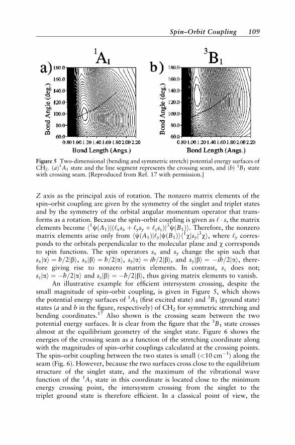
Z axis as the principal axis of rotation. The nonzero matrix elements of thespin–orbit coupling are given by the symmetry of the singlet and triplet statesand by the symmetry of the orbital angular momentum operator that trans-forms as a rotation. Because the spin–orbit coupling is given as ‘ � s, the matrixelements become h1cðA1Þjð‘xsx þ ‘ysy þ ‘zszÞj3cðB1Þi. Therefore, the nonzeromatrix elements arise only from hcðA1Þj‘yjcðB1Þih1wjsyj3wi, where ‘y corres-ponds to the orbitals perpendicular to the molecular plane and w correspondsto spin functions. The spin operators sx and sy change the spin such thatsxjai ¼ �h=2jbi, sxjbi ¼ �h=2jai, syjai ¼ i�h=2jbi, and syjbi ¼ �i�h=2jai, there-fore giving rise to nonzero matrix elements. In contrast, sz does not;szjai ¼ ��h=2jai and szjbi ¼ ��h=2jbi, thus giving matrix elements to vanish.

An illustrative example for efficient intersystem crossing, despite thesmall magnitude of spin–orbit coupling, is given in Figure 5, which showsthe potential energy surfaces of 1A1 (first excited state) and 3B1 (ground state)states (a and b in the figure, respectively) of CH2 for symmetric stretching andbending coordinates.17 Also shown is the crossing seam between the twopotential energy surfaces. It is clear from the figure that the 3B1 state crossesalmost at the equilibrium geometry of the singlet state. Figure 6 shows theenergies of the crossing seam as a function of the stretching coordinate alongwith the magnitudes of spin–orbit couplings calculated at the crossing points.The spin–orbit coupling between the two states is small (<10 cm�1) along theseam (Fig. 6). However, because the two surfaces cross close to the equilibriumstructure of the singlet state, and the maximum of the vibrational wavefunction of the 1A1 state in this coordinate is located close to the minimumenergy crossing point, the intersystem crossing from the singlet to thetriplet ground state is therefore efficient. In a classical point of view, the

Figure 5 Two-dimensional (bending and symmetric stretch) potential energy surfaces ofCH2: ðaÞ1A1 state and the line segment represents the crossing seam, and (b) 3B1 statewith crossing seam. [Reproduced from Ref. 17 with permission.]


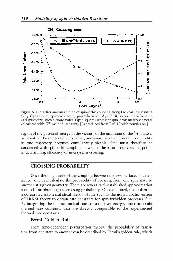
region of the potential energy in the vicinity of the minimum of the 1A1 state isaccessed by the molecule many times, and even the small crossing probabilityin one trajectory becomes cumulatively sizable. One must therefore beconcerned with spin–orbit coupling as well as the location of crossing pointsin determining efficiency of intersystem crossing.

CROSSING PROBABILITY

Once the magnitude of the coupling between the two surfaces is deter-mined, one can calculate the probability of crossing from one spin state toanother at a given geometry. There are several well-established approximationmethods for obtaining the crossing probability. Once obtained, it can then beincorporated into a statistical theory of rate such as the nonadiabatic versionof RRKM theory to obtain rate constants for spin-forbidden processes.18–20

By integrating the microcanonical rate constant over energy, one can obtainthermal rate constants that are directly comparable to the experimentalthermal rate constants.

Fermi Golden Rule

From time-dependent perturbation theory, the probability of transi-tion from one state to another can be described by Fermi’s golden rule, which

Figure 6 Energetics and magnitude of spin–orbit coupling along the crossing seam inCH2: Open circles represent crossing points between 1A1 and 3B1 states in their bendingand symmetric stretch coordinates. Open squares represent spin–orbit matrix elementscalculated with Zeff method (see text). [Reproduced from Ref. 17 with permission.]


says that the probability is given by the square of the transition matrix ele-ment. In the case of a spin-forbidden reaction, the crossing probability is givenby the square of the spin–orbit matrix elements, which is expressed as

P ¼ 2p�h

Xf

jh�f jHSOj�iihwf jwiij2 ½5�

Here hwf jwii is the Franck–Condon factor that represents the overlap of thevibrational wave functions of the initial and final states. The geometry depen-dence of the spin–orbit coupling is neglected in this case. Therefore, the con-tributing factor for spin-forbidden transitions is having not only spin–orbitcoupling nonzero and the crossing point energetically accessible, but alsoensuring that the vibrational wave functions have nonzero overlap.

Landau–Zener Semiclassical Approximation

In this approximation, the probability of transition is given by Eq. [6]

P ¼ e�2g ½6�

In this equation, g is a so-called Massey parameter that is defined as

g ¼ �h

2m

jh�f jHSOj�iij2

�gfiv½7�

where v is the velocity of the particle with mass m passing through the crossingpoint, and �gfi is the difference in the gradients of the two potential energysurfaces at the crossing point. Since the Landau–Zener approximation isderived from a semiclassical approximation, the tunneling contribution belowthe crossing point energy is not included, and it is known21–23 that the transi-tion probability calculated using the Landau–Zener treatment in this region isunderestimated. Above the crossing point energy, the approximation givesgood results. Generalization of the Landau–Zener method is reviewed byNakamura in his monograph.23

METHODOLOGIES FOR OBTAINING SPIN–ORBITMATRIX ELEMENTS

In this section, relativistic quantum mechanics and methods for calculat-ing the spin–orbit matrix elements are presented. Excellent reviews of thismaterial have been published by Almlof and Gropen24 and Hess et al.25 The

Methodologies for Obtaining Spin–Orbit Matrix Elements 111

basic theory of relativistic quantum mechanics is presented in many texts, suchas those in Ref. 26.

Electron Spin in Nonrelativistic Quantum Mechanics

The classic experiments of Stern and Gerlach showed that a beam of sil-ver atoms (later confirmed for hydrogen atoms) in an inhomogeneous mag-netic field gave rise to two distinct spots on the photographic plate, insteadof a broadened spot as expected from classical mechanics. In addition, themultiplet structure appears in atomic spectra when a weak magnetic field isapplied. These results indicate that electrons possess magnetic angularmomentum and they are quantized to two distinct states.

The spin angular momentum has homologous properties to the orbitalangular momentum, namely,

½sx; s2� ¼ ½sy; s

2� ¼ ½sz; s2� ¼ 0 ½8�

½sx; sy� ¼ i�hsz ½9�½sy; sz� ¼ i�hsx ½10�½sz; sx� ¼ i�hsy ½11�

s2 ¼ s2x þ s2

y þ s2z ½12�

To match the two-valuedness of the electron spin and the commutating prop-erties shown above, Pauli introduced spin matrices, si. Each component ofspin can then be written in terms of the 2� 2 spin matrices,

sx ¼1

2�hsx ½13�

sy ¼1

2�hsy ½14�

sz ¼1

2�hsz ½15�

Then the eigenvalue of the si is þ1. Because the spin matrices are 2� 2matrices, the internal state of electrons must be represented by two-columnmatrices,

cPðr;msÞ ¼cþðrÞc�ðrÞ

� �½16�

where cP is Pauli’s spinor (spin orbital). If ms ¼ þ 12, then �� ¼ 0, and if

ms ¼ � 12, then �þ ¼ 0. The Pauli spinor can then be represented as

cPðr;msÞ ¼ cþðrÞwðmsÞ þ c�ðrÞwðmsÞ ½17�


where w is the spin function that depends only on ms, and

w þ 1

2

� �¼

1

0

� �½18�

w � 1

2

� �¼

0

1

� �½19�

The complex conjugate of the Pauli spinor is given by a two-row matrix,

c�Pðr;msÞ ¼ ðc�þðrÞ c��ðrÞÞ ½20�

Therefore, the spin operators must be 2 2 matrices. When the eigenvalue iseither �1 or þ1 assuming that the quantization is observed in the z direction,it is readily seen that

sz ¼1 00 �1

� �½21�

Furthermore, consistency in the commutation relations is only achieved byhaving

sx ¼0 1

1 0

� �½22�

sy ¼0 i

�i 0

� �½23�

By using the spin matrices, the two-valuedness of an electron can be incorpo-rated into the Schrodinger equation. For a hydrogen-like atom, one can writethe Schrodinger equation in the form,

ðspÞ ðspÞ2m

þ V

� �cP ¼

1

2m

pz px þ ipy

px � ipy �pz

� �2

þV

" #cP ¼ EcP ½24�

where p and pi are the vector and ith component of the scalar form of themomentum operators, respectively, V is the Coulomb potential, and cP isthe Pauli spinor comprised of two components. The kinetic energy part ofEq. [24] reduces to the usual ð2mÞ�1ðp2

x þ p2y þ p2

z Þ, except that we have twocomponents corresponding to the electron spin. In nonrelativistic theory, elec-tron spin is incorporated into the Schrodinger equation in this fashion.


Klein–Gordon Equation

According to the special theory of relativity, all physical laws are postu-lated to be invariant in any inertial frame of reference. Furthermore, the equa-tions of motion must be invariant under a Lorentz transformation,

x0 ¼ 1

ð1� v2=c2Þ1=2ðx� vtÞ ½25�

t0 ¼ 1

ð1� v2=c2Þ1=2ðt � vx=c2Þ ½26�

where x is position, v is velocity, c is the speed of light, and t is time. Primes onthe left-hand side indicate a different reference frame from the quantity with-out the prime. From these equations, it is clear that when a particle is travelingat a small fraction of the speed of light, that is, where the v2=c2 term is small,Eqs. [25] and [26] reduce to the classical Galilean transformation equations.

Another requirement in satisfying the special theory of relativity is tohave the spatial and temporal variables being treated on the same footing.The differential operators in Lorentz invariant form are q/qx, q/qy, q/qz, and(1/ic)q/qt, giving the magnitude for spatial and temporal dimensions asx2 þ y2 þ z2 � c2t2. This means that the order of the differentials for the coor-dinate and time in the equation of motion must be the same. The time-dependent Schrodinger equation exhibits time derivatives in the first orderand coordinate derivatives in the second order; therefore it is not Lorentzinvariant.

The classical relativistic energy of a free particle moving in space isgiven as

E ¼ffiffiffiffiffiffiffiffiffiffiffiffiffiffiffiffiffiffiffiffiffiffiffiffiffiffip2c2 þm2c4

p½27�

which relates rest mass and the kinetic energy of a particle. By using the rela-tion E! i�hq=qt from the Schrodinger correspondence rule, and substituting itinto the time-dependent Schrodinger equation, the relativistic quantummechanical equation of a free particle may be written as

��h2 q2cðx; tÞqt2

¼ ½p2c2 þm2c4�cðx; tÞ ½28�

This equation is called the Klein–Gordon equation. The Klein–Gordon equa-tion satisfies the order of the differentials to be in the same order for space andtime, and thus is Lorentz invariant. This equation, however, does not giverise to a positive definite density due in part to the second-order differentialin time. Furthermore, for a fermion system, the Klein–Gordon equation is


not adequate since it contains no properties of spin that can be derivednaturally.

Dirac Equation

Dirac was seeking an equation that is analogous to the Schrodinger equa-tion, with a first-order derivative in time, and simultaneously satisfying theLorentz invariance. He took a bold step: If the relativistic energy, the expres-sion under the radical in the energy expression (Eq. [27]) or in the squarebracket (Eq. [28]), is factored into a perfect square such that

E2 ¼ p2c2 þm2c4 ! E ¼ ðpcÞ þmc2 ½29�

the Hamiltonian can then be expressed as

HD ¼ ca � pþ bmc2 ½30�

This is called the Dirac Hamiltonian. To obtain the correct mathematics,Dirac introduced parameters a and b. Then, by expanding out all termsin the four dimensions (originally thought of as spatial and temporal dimen-sions) the parameters, a and b, must anticommute and their squares must beunity. The choice of a and b must then be that

a1¼

0 0 0 10 0 1 00 1 0 01 0 0 0

0BB@

1CCA a2¼

0 0 0 �i0 0 i 00 �i 0 0i 0 0 0

0BB@

1CCA a3¼

0 0 1 00 0 0 �11 0 0 00 �1 0 0

0BB@

1CCA b¼

1 0 0 00 1 0 00 0 �1 00 0 0 �1

0BB@

1CCA

½31�

Then, the time-dependent wave equation is, written as

i�hq�ðx; tÞ

qt¼ ðca � pþ bmc2Þ�ðx; tÞ ½32�

Therefore, the four components of the Hamiltonian must give rise to fourcomponents to the wave functions. The off-diagonal blocks of ai above arethe corresponding Pauli spin matrices (Eqs. [22], [23], and [21], respectively).Therefore, the four components of the wave function contain electron spin as anatural extension of the Klein–Gordon equation. Given these choices, thetime-dependent wave equation for a free particle is rigorously Lorentz invar-iant. Furthermore, it turns out that the four-component Dirac equation givesrise to positive and negative eigenstates, and the two contain the electronic andpositronic solutions, respectively.


For hydrogen and hydrogen-like atoms, the Dirac Hamiltonian musthave the form,

HD ¼ ca � pþ bmc2 þ V ½33�

where V is the interaction potential of an electron with a point nucleus. Therelativistic correction to the interaction potential is small (order of 1/c3) and isusually ignored. If the potential contains electron–electron Coulombic interac-tions just as in a many-electron atom, the Hamiltonian is no longer Lorentzinvariant; nonetheless, the Coulomb interaction is often used. The rationalefor the molecular four-component Dirac calculation using the usual Coulombinteractions is that the magnitude of the Lorentz variance is of relatively smallimportance. Analogous to the Hartree–Fock method in nonrelativistic theory,the Dirac equation for many-electron systems can be cast into one-particleoperators utilizing the antisymmetrized product functions. This type of theoryis called Dirac–Fock (or Dirac–Hartree–Fock) theory.27 More specifically, if aCoulomb potential is used, it is referred to as Dirac–Coulomb theory. In addi-tion to single configuration theory, a multiconfigurational self-cosistent field(MCSCF) variant also exists.28 Dynamical electron correlation can also beincluded in the calculations by CI, many-body perturbation theory, andcoupled-cluster theory (CCSD).29d,e

The Coulomb interaction, however, can be corrected for relativistic con-straints with approximate solution good to 1=c2. This so-called Breit interac-tion is given by30

VBreit12 ¼ 1

r12� 1

2r12a1 � a2 þ

ða1 � r12Þða1 � r12Þr212

� �½34�

where the first and second terms in the brackets on the right-hand side ofEq. [34] are known as the Gaunt interaction and retardation terms, respec-tively. Depending on the type of electron–electron interaction used in thecalculations, the corresponding single configuration theory is called, Dirac–Breitor Dirac–Gaunt theory. Further details on these theories are reviewed in Ref. 29.

The eigenspectrum of the four-component Dirac equation is given by thepositive and negative eigenstates centered at the quantity �mc2. The positiveenergy solution is the electron solution, while the negative energy solution isfor positrons. The wave functions associated with the Dirac equation containfour components, as mentioned earlier. For the positive energy (electronic)solution, two components are larger than the other two components. Thetwo large components for the positive solution become the small componentwhen solving for positron states. In the nonrelativistic limit, assuming thewave function to be hydrogen-like, the small component, �S, is shown31 tobe a small fraction of the large component, �L, by

�S �Z

2c�L ½35�


For the solution to the electronic problem, the two components of the Diracspinors are larger by a factor Z/2c, and a natural question to ask is whetherthere exists a separable solution to describe only electronic solutions. Thisquestion is addressed below.

Foldy–Wouthuysen Transformation

As described above, the nonrelativistic Pauli wave function consists oftwo component spinors. It would be of interest to see if the Dirac equationcan be reduced to two-component equations since we are specifically inter-ested in the solution to the electronic problem, particularly given that the smallcomponent of the Dirac functions are on the order of Z/2c. Furthermore, com-putational effort is much smaller in two-component solutions than in four-component solutions. The following derivation is due to Greiner.26a

Consider first a free particle case. The Dirac equation of a free particlecan be written as

mc2 ca � pca � p �mc2

� ��þ��

� �¼ E

�þ��

� �½36�

where �þ and �� represent the wave functions corresponding to large andsmall components. If a transformation is performed such that the off-diagonalterm in the transformed Hamiltonian becomes zero, Eq. [36] separates intolarge and small components. Foldy and Wouthuysen32 devised a unitary trans-formation that results in the block diagonal form of the Dirac equation; there-fore one can obtain a solution containing only the electronic components. Theunitary operator for such a transformation has the form

U ¼ eiS ½37�

and,

UyU ¼ e�iSeiS ¼ 1 ½38�

For a free electron, if the S operator is chosen to have the following form inmomentum space,

S ¼ � i

2mc

� �ba � po p

mc

� �½39a�

where

o ¼ mc

ptan�1 p

mc

� �½39b�

the free-particle Dirac Hamiltonian, Eq. [30], can then be shown to give

Hf ¼ UyHDU ¼ e2iSðca � pþ bmc2Þ ½40�


By expanding e2iS in a Taylor series and collecting the even and odd powers ofthe expansion terms, one can relate these terms to a trigonometric expansion,such that

e2iS ¼ cosp

mco

� �þ b

a � pp

sinp

mco

� �� ½41�

Then, Eq. [40] can be shown to be exactly

Hf ¼ bEp ½42�

where Ep is the free electron kinetic energy of Eq. [27].In the presence of a Coulomb potential, there is no exact solution as we

found for the free-particle case. By choosing a certain unitary operator, onecan systematically reduce the coupling between the large and small compo-nents. The Hamiltonian is first decomposed into parts,

H ¼ bmc2 þ eþO ½43�

where e and O are the even and odd operators, and they are in general

e ¼ eVðrÞ ½44�

O ¼ ca p� e

cA

� �½45�

where A is the vector potential. The exponential unitary operator, Eq. [37], isused here with the similar choice of S, given by

S ¼ � i

2mc2bO ½46�

With this choice of the S operator, the unitary transformation is performed,such that

H0 ¼ UyHU ¼ 1þ iS

1!þ i2S2

2!þ � � �

� �H 1� iS

1!þ i2S2

2!� � � �

� �½47�

Here the exponential operator is expanded in a power series. The transformedHamiltonian can be written in terms of commutators in the usual sense, that is,½a; b� ¼ ab� ba (therefore, ½a; ½b; c�� ¼ ½a; ðbc� cbÞ� ¼ abc� bca� acbþ cba),as,

H0 ¼ H þ i½S;H� þ i2

2½S; ½S;H�� þ i3

3!½S; ½S; ½S;H�� þ � � � ½48�


By expanding out the commutators up to the order 1/m3c6, one finds

i½S;H� ¼ �Oþ bO2

mc2þ b

2mc2½O; e� ½49�

i2

2½S; ½S;H�� ¼ � 1

2mc2bO2 � 1

2m2c4O3 � 1

8m2c4½O; ½O; e�� ½50�

i3

3!½S; ½S; ½S;H�� ¼ � 1

6m2c4O3 � 1

6m2c4bO4 � 1

48m3c6b½O; ½O; ½O; e�� ½51�

i4

4!½S; ½S; ½S; ½S;H�� 1

24m3c6bO4 ½52�

By substituting the commutators, Eqs. [49]–[52], into Eq. [48] one arrives at

H0 ¼ bmc2þ bO2

2mc2� bO4

8m3c6þ e�½O; ½O;e��

8m2c4þb½O;e�

2mc2� O3

3m2c4�b½O; ½O; ½O;e��

48m3c6

½53�

The next step is to further reduce the terms with odd powers of the O opera-tors, which can be accomplished by another unitary transform using the S0

operator,

S0 ¼ � i

2mc2bO0 ½54�

where O0 is the odd powers of the O operators appearing in the transformedHamiltonian H0 (Eq. [53]) neglecting the last term due to large powers of1/mc2, given as

O0 ¼ b½O; e�2mc2

� O3

3m2c4½55�

With the choice of S0 the, Hamiltonian H0 is transformed into H00 as

H00 ¼ eiS0H0e�iS0 ¼ bmc2 þ e0 þ b½O0; e0�2mc2

� O03

3m2c4½56�

where e0 is e plus the operators of even powers of O in H0 (Eq. [53]). The lastterm containing O03 can be neglected because that term contains large powersof 1/mc2. Further reduction is achieved by another unitary transformationusing

S00 ¼ � i

2mc2bO00 ½57�

where O00 contains the terms with odd powers of O in H00 (Eq. [56]). Then, onefinally arrives at

H000 ¼ bmc2 þ e0 ¼ bmc2 þ bO2

2mc2� bO4

8m3c6þ e� ½O; ½O; e��

8m2c4½58�


The Hamiltonian H000 now contains only even powers of the O operators.When each term of the transformed Hamiltonian H000 is expanded, one obtainsthe so-called Breit–Pauli Hamiltonian.

For a many-electron system, one starts with the Breit equation, instead ofEq. [33]. The Breit equation includes the relativistic correction terms, Eq. [34],for electron–electron interactions, and is given as

E�HDi �e2

rij

� �� ¼ � e2

2rijai � aj þ

ðai � rijÞ � ðaj � rijÞr2ij

" #� ½59�

Here HDi is the Dirac Hamiltonian for a single particle, given by Eq. [30].Recall from above that the Coulomb interaction shown is not strictly Lorentzinvariant; therefore, Eq. [59] is only approximate. The right-hand side of theequation gives the relativistic interactions between two electrons, and is calledthe Breit interaction. Here ai and aj denote Dirac matrices (Eq. [31]) forelectrons i and j. Equation [59] can be cast into equations similar to Eq.[36] for the Foldy–Wouthuysen transformation. After a sequence of unitarytransformations on the Hamiltonian (similar to Eqs. [37]–[58]) is applied toreduce the off-diagonal contributions, one obtains the Hamiltonian in termsof commutators, similar to Eq. [58]. When each term of the commutatorsare expanded explicitly, one arrives at the Breit–Pauli Hamiltonian, HBP, fora many-electron system33,34

HBP ¼X6

i¼1

HBPi ½60�

HBP1 ¼

e2�h

2m2e c2

Xi;a

Za

r3ia

ðri;a � piÞ � si �Xi;j 6¼i

ðrij � piÞ � ðsi þ 2sjÞ" #

½61�

HBP2 ¼

e2�h

2m2e c2

Xi;j6¼i

jrijj2si � sj � 3ðrij � siÞðrij � sjÞjrijj5

� e2�h

2m2e c2

8p3

Xi;j6¼i

dðrijÞsi � sj ½62�

HBP3 ¼ �

e2�h

4m2e c2

Xi;a

Za

jriaj3ria � pi �

Xi;j 6¼i

1

jrijj3rij � pi

" #½63�

HBP4 ¼ �

e2�h

4m2e c2

Xi;j

pi � pj

jrijjþ½rij � ðrij � pjÞpi�

jrijj3

" #½64�

HBP5 ¼ �

1

8m3e c2

Xi

p4i ½65�

HBP6 ¼

e�h

2m2e c2

Xi

½ðEi � piÞ � si� �ie�h

4m2e c2

Xi

ðEi � piÞ þe�h

mc

Xi

ðHi � siÞ ½66�


The first term, HBP1 , is the spin–orbit (one electron term) and spin–other-orbit

(two electron term) couplings, which are the topic of the following subsection.The second term HBP

2 contains the spin–spin coupling term and Fermi contactinteraction. Both the HBP

1 and HBP2 can lift degeneracy in multiplets. The para-

meter HBP3 is the Dirac correction term for electron spin and HBP

4 is the classicalrelativistic correction to the interaction between electrons due to retardationof the electromagnetic field produced by an electron. The parameter HBP

5 isthe so-called mass-velocity effect, due to the variation of electron mass withvelocity. Finally, HBP

6 is the effect of external electric and magnetic fields.An alternative formulation35 that one can use to obtain the Breit–Pauli

Hamiltonian is to start with the Breit equation (Eq. [59]). The equation is firsttransformed by Fourier transformation to momentum space. The terms invol-ving the positive and negative eigenstates into Pauli functions cþ and c� arethen written, and only the electronic part of the equations is kept. Then,expanding the energy (in momentum space) in powers of p/mc, and Fouriertransforming back to the coordinate space, one finally arrives at a differentialequation of the form containing the Breit–Pauli Hamiltonian.

Breit–Pauli Hamiltonian

The most popular way in which nonscalar relativistic effects, such asspin–orbit coupling, are incorporated into molecular calculations, is to usethe Breit–Pauli Hamiltonian. This approach is most convenient, because therelativistic effects under consideration can be added to the nonrelativisticHamiltonian after the zeroth-order wave function is determined. By utilizingperturbation theory, or during the calculation of the electron correlation withprocedures, such as MCSCF or CI, spin–orbit coupling matrix elements andassociated wave functions can be calculated. Algorithm development utilizingthe Breit–Pauli Hamiltonian in terms of perturbation theory have beendiscussed in detail by Langhoff and Kern,33 Yarkony,34 Furlani and King,36

and Federov and Gordon.37

The scalar relativistic corrections of the Breit–Pauli Hamiltonian, HBP3 ,

HBP4 , and HBP

5 , gives rise to atomic properties such as core orbital contractionand f-orbital expansion observed in experiment, therefore affecting geometryin molecular calculations. However, the Breit–Pauli operators containingterms with higher powersof r�n give a singularity near thenucleus which is, at least,‘‘more’’ singular than the 1/r term of Coulombic interaction. In many applications,however, particularly of molecules containing light elements, the singularity is gen-erally avoided due to truncation of the basis set expansion to a finite set.

Zeff Method

The first approximation method for the Breit–Pauli spin–orbit Hamilto-nian is to neglect the contribution from the two-electron terms. Justification


for such an omission is that the two-electron terms are relatively small, at leastfor lighter elements. To compensate for the small error that is created byneglecting the two-electron term, the effective nuclear charge Zeff is intro-duced.38 The spin–orbit Hamiltonian is then given by

HSO ¼ a2

2

Xne

i

XNA

ZeffA

r3iA

‘iA � si ½67�

where a is the fine-structure constant, and ZeffA is the effective nuclear charge of

the atom A. Koseki et al.7,8,39 examined the magnitude of Zeff for the maingroup elements systematically. They adjusted the Zeff so that the fine-structuresplitting of spectral terms of diatomic hydrides is reproduced by utilizingthe MCSCF/SBKJC method. SBKJC uses the effective core potentials and thecorresponding basis sets of Stevens et al.40 The proposed equation for theeffective nuclear charge is

Zeff ¼ Z � fk ½68�

where k ¼ 1–6, denotes the kth row of the periodic table. The parameters fk

for each row of the periodic table are determined to be

f1 ¼ 1 for H

f2 ¼ 0:45þ 0:05m

f3 ¼ 12

f4 ¼ 41 ð f4 ¼ 11 for GaÞf5 ¼ 110 ð f5 ¼ 33 for InÞf6 ¼ 222 ð f6 ¼ 113 for TlÞ

Here m is the number of valence electrons.The effective nuclear charge for transition metals7 is determined from the

atomic spectral terms10 because few experimental data on diatomic transitionmetal hydrides are available (see e.g., Ref. 41). The effective nuclear chargesdetermined for transition elements are given by

Zeff ¼ Z � f TMk ½69�

where

f TM4 ¼ 0:385þ 0:025 ðm� 2Þ

f TM5 ¼ 4:680þ 0:060 ðm� 2Þ

f TM6 ¼ 13:960þ 0:140 ðm� 2Þ


Here m is the number of electrons occupying the nd and (nþ 1Þs orbitals in aneutral atom. The value of m can assume a number 1–9. The group 12 (IIB)elements, Zn, Cd, and Hg, have filled d orbitals, so that Zeff values were deter-mined to be in a different category. Even though the 3d SBKJC pseudo-orbitalsare qualitatively similar to the correct 3d atomic orbitals, the 4d and 5dSBKJC pseudo-orbitals are nodeless and, as a result, large Zeff values are givento the second- and third-row elements. Such large Zeff values lose theirphysical meaning and are recognized as simply being empirical parameters.A similar approach has been taken by several authors in the past11,38 fordifferent systems, like carbon and silicon atoms, and used for atom–rare gascollisions.

Effective Core Potential-Based Method

Three key review articles exist that describe the derivation and utilizationof the ECP method.42–44 For a molecular system containing atoms of largeZ, an all-electron calculation is a formidable task. Furthermore, for suchmolecules one must contend with scalar relativistic effects, such as thecore-orbital contraction due to mass-velocity and Darwin terms that lead togeometry changes in molecules, in addition to spin–orbit coupling effects.The relativistic effective core potential replaces core electrons by a potential,but implicitly incorporates scalar relativistic effects through a fit of the corepotential to the atomic Dirac–Fock results. For general applications, the rela-tivistic effective potential is averaged over two spin states for a given l therebyaveraging out the effect of spin–orbit coupling.45,46

The relativistic effective potential UREP is the j (total angular momen-tum) dependent core potential fit to the large component of the Dirac four-component wave functions. The average relativistic effective potential UAREP

is the average relativisitic potential of the j states, given as

UAREP‘ ¼

‘UREP‘;‘�1=2 þ ð‘þ 1ÞUREP

‘;‘þ1=2

2‘þ 1½70�

Because UAREP is constructed from a potential fit to the Dirac four-componentwave functions, it contains all relativisitic effects, except for spin–orbit cou-pling. The spin–orbit coupling operator for the effective core potential isthen given as the difference between the relativistic effective potential, UREP,and the averaged relativistic effective potential, UAREP,

HSO ¼ UREP �UAREP ½71�


The spin–orbit operator can be shown to be

HSO ¼XL�1

‘¼1

�UREP‘ ðrÞ

�‘

2‘þ 1

X‘þ1=2

�‘�1=2

��‘; ‘þ 1

2;m

��‘; ‘þ 1

2;m

�� ‘þ 1

2‘þ 1:

X‘�1=2

�‘þ1=2

��‘; ‘� 1

2;m

��‘; ‘� 1

2;m

��

½72�

where �UREP ðrÞ is given as

�UREP‘ ðrÞ ¼ UREP

‘;‘þ1=2 �UREP‘;‘�1=2 ½73�

The spin–orbit operator, Eq. [72], is constructed from the effective corepotentials.

The spin–orbit coupling is incorporated into the calculations at the post-Hartree–Fock level, particularly with CI. This is generally referred to as spin–orbit CI. The core potential and associated basis sets for Li��Kr, including thespin–orbit operator, have been published.47–50 Implementation of the spin–orbit CI method has been discussed by Pitzer and co-workers.51–53 It hasalso been reported that the spin–orbit CI code has been adapted to a parallelcomputing enviroment.54

Model Core Potential-Based Method

Model core potential (MCP) methods55 replace core orbitals by a poten-tial just as in ECP. On the other hand, MCP valence orbitals preserve the nodalstructure of valence orbitals, unlike ECP valence orbitals. The expectationvalues of hr�3i for the valence orbitals show that the results of MCP are closerto those calculated with all-electron orbitals when comparing MCP, ECP, andthe all electron case.56 Comparisons between MCP and an all electron basisutilizing the full Breit–Pauli spin–orbit Hamiltonian based on multiconfigura-tional quasidegenerate perturbation theory (MCQDPT) calculations showgood agreement between the two methods for hydrides of P, As, and Sb.57

The MCP based spin–orbit calculation appears to be a promising technique,but systematic studies of many different molecular systems are still neededto assess its characteristics and accuracy.

Douglas–Kroll Transformation

The singularity that may arise when using the Breit–Pauli Hamiltoniancan cause instability in variational calculations and it is desirable that such sin-gularity be avoided formally. Douglas and Kroll58 showed that the singularity


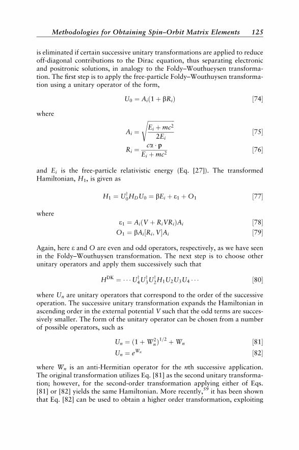
is eliminated if certain successive unitary transformations are applied to reduceoff-diagonal contributions to the Dirac equation, thus separating electronicand positronic solutions, in analogy to the Foldy–Wouthueysen transforma-tion. The first step is to apply the free-particle Foldy–Wouthuysen transforma-tion using a unitary operator of the form,

U0 ¼ Aið1þ bRiÞ ½74�

where

Ai ¼

ffiffiffiffiffiffiffiffiffiffiffiffiffiffiffiffiffiffiffiEi þmc2

2Ei

s½75�

Ri ¼ca � p

Ei þmc2½76�

and Ei is the free-particle relativistic energy (Eq. [27]). The transformedHamiltonian, H1, is given as

H1 ¼ Uy0HDU0 ¼ bEi þ e1 þO1 ½77�

where

e1 ¼ AiðV þ RiVRiÞAi ½78�O1 ¼ bAi½Ri;V�Ai ½79�

Again, here e and O are even and odd operators, respectively, as we have seenin the Foldy–Wouthuysen transformation. The next step is to choose otherunitary operators and apply them successively such that

HDK ¼ � � �Uy4Uy3Uy2H1U2U3U4 � � � ½80�

where Un are unitary operators that correspond to the order of the successiveoperation. The successive unitary transformation expands the Hamiltonian inascending order in the external potential V such that the odd terms are succes-sively smaller. The form of the unitary operator can be chosen from a numberof possible operators, such as

Un ¼ ð1þW2nÞ

1=2 þWn ½81�Un ¼ eWn ½82�

where Wn is an anti-Hermitian operator for the nth successive application.The original transformation utilizes Eq. [81] as the second unitary transforma-tion; however, for the second-order transformation applying either of Eqs.[81] or [82] yields the same Hamiltonian. More recently,59 it has been shownthat Eq. [82] can be used to obtain a higher order transformation, exploiting


the exponential expansion of anti-Hermitian operators cast into commutatorforms, as seen above for transforming Eq. [47] into Eq. [48]. Other closelyrelated approaches have been explored by Dyall.60

In most current applications of the Douglas–Kroll transformation, theHamiltonian is truncated at second order in the successive unitary transforma-tion, that is, HDK2 ¼ Uy2H1U2, and the resulting Hamiltonian can be written interms of spin-free and spin-dependent components,

HDK2 ¼ Uy2H1U2 ¼X

i

ðEi þ Veffi Þ þ

Xi6¼j

Veffij þ

Xi

HSOi þ

Xi 6¼j

HSOij ½83�

where the summation terms are one-electron spin-free, two-electron spin-free,one-electron spin–orbit, and two-electron spin–orbit terms, respectively. Theeffective potentials for spin-free terms are given by

Veffi ¼ Ai½V þ RiVRi�Ai �

1

2ffEi;W1g;W1g ½84�

Veffij ¼ AiAj

e2

rijþ Ri

e2

rijRi þ Rj

e2

rijRj þ RiRj

e2

rijRiRj

� �Ai;Aj ½85�

and where

W1 ¼ AiðQi �Q0iÞA0iVðpi; p

0iÞ

Ei � E0i½86�

Here, Eq. [86] is an integral equation with a kernel, and Vðpi; p0i) is the poten-

tial energy operator in momentum space. The curly bracket in Eq. [84] denotesthe anticommutator, where fa; bg ¼ abþ ba. Implementation of the spin-freepart of the Hamiltonian is generally given only to the one-electron term,Eq. [84], and for electron– electron repulsion61 is usually ignored. Incorpora-tion of the DK Hamiltonian to existing electronic structure theory code is thenrelatively straightforward by adding one new type of one-electron integral(all others can be obtained from the existing nonrelativistic code).62

The spin-dependent part of Eq. [83] is the one-electron and two-electronspin–orbit operators,

HSOi ¼ e2Za

Ai

Ei þmc2si

ria

r3ia

� pi

� �Ai

Ei þmc2½87�

HSOij ¼ �e2 AiAj

Ei þmc2

rij

r3ij

� pi

!� ðsi þ 2sjÞ

AiAj

Ei þmc2½88�

The spin–orbit operators in the Douglas–Kroll Hamiltonian still contain the1/r3 term; however, that term is offset by the 1/(Ei þmc2) term, where as


ri ! 0, pi !1. Therefore, the spin–orbit operators in the Douglas–KrollHamiltonian are stable in the variational calculations.

The spin-free Douglas–Kroll Hamiltonian has been implemented in pub-lically available electronic structure codes,63 and has been utilized for comput-ing properties of molecules containing heavy atoms. Electron correlation canbe evaluated once the spin-free DK orbitals are formed, just as in nonrelativis-tic post-Hartree–Fock methods, with only small modification to the code.For example, coupled cluster theory has been implemented as a post-DKmethod.64 Furethermore, the spin-free ab initio model core potential (AIMP),65

based on the DK3 Hamiltonian, has been developed for the actinide elementsby Paulovic et al.66 On the other hand, the spin-dependent Douglas–KrollHamiltonian has been implemented only in a few codes, and therefore the uti-lity of the formalism is currently limited in scope. Hess et al.25 reviewed theirresults on transition metal containing diatomics and small polyatomic mole-cules. Their work is one of only a few studies carried out for DK spin–orbitcoupling. Fedorov, Nakajima, and Hirao used the DK3 spin-free Hamiltonianand the one-electron spin–orbit DK Hamiltonian plus the two-electron Breit–Pauli spin–orbit operator to investigate the uranium atom and uraniumfluoride.67

The treatment of spin–orbit coupling can be incorporated into molecularcalculations in the form of atomic mean-field spin–orbit integrals (AMFI).68

Because the method is a mean-field approach, the original formulation waslimited to spin–orbit splitting in a single state. Later, MCSCF methodologyin the framework of a restricted active space was used to obtain interstatespin–orbit coupling, thereby enabling examination of coupling between statesof different spins.69

New transformation formalisms for obtaining two component equationsare currently being investigated and being applied to atomic systems.70 Suchstudies and others71 together with implementation of the Douglas–Krollspin–orbit Hamiltonian, give special importance to this active field ofrelativistic quantum chemistry.

POTENTIAL ENERGY SURFACES

The potential energy surfaces of two states of different symmetry andspin can cross in Nint � 1 dimensions, where Nint is the number of internalcoordinates (one coordinate as a constraint to have the same energy). There-fore, in general, the potential energy crossing forms a hypersurface asdescribed earlier in this chapter. A priori determination of the MEXP on thehypersurface is highly desirable through analytical gradient techniques by ana-logy to locating a transition state in adiabatic reactions. In what is to follow,minimum energy crossing point location algorithms are discussed.

Potential Energy Surfaces 127

Minimum Energy Crossing-Point Location

A procedure for locating a minimum energy crossing point between twopotential energy surfaces closely follows the geometry optimization techniquesavailable in most modern electronic structure theory codes.2b In essence, a sta-tionary point is searched by means of an iterative Newton–Raphson procedurewhereby the knowledge of gradients and the Hessian at a current point of eva-luation gives a displacement vector to which the next evaluation of the gradi-ent and Hessian is to be carried out. For an adiabatic potential energy surface,the potential energy is expanded in a Taylor series to the linear term; the linearNewton–Raphson equation is then obtained

gIðRÞdR ¼ �EIðRÞ ½89�

Here, gIðRÞ is the gradient evaluated at nuclear coordinate R, and EIðRÞ is theIth state energy. Given the fact that the gradient itself can also be expanded ina Taylor series, one can utilize the recursion to obtain the more familiar quad-ratic Newton–Raphson equation,

QIðRÞdR ¼ �gIðRÞ ½90�

where QIðRÞ is the Hessian and gIðRÞ is the gradient evaluated at the currentpoint R. At convergence, the predicted displacement dR meets a preset conver-gence criterion. Instead of calculating the Hessian at every iteration, variousHessian updating procedures can be used to avoid relatively expensive Hessiancalculations.1a

Koga and Morokuma72 treated the MEXP search as a constrained opti-mization. In their Lagrange multiplier method, the energy of the Ith state,EIðRÞ, is minimized with a constraint that the energy difference betweentwo states, I and J, becomes zero. The Lagrangian is written as

LðR; lÞ ¼ EIðRÞ þ l½EIðRÞ � EIðRÞ� ½91�

The Lagrangian is expanded in a Taylor series, analogous to Eq. [90] above,and one obtains the Newton–Raphson equation for the Lagrangian,

QIJðR; lÞ gIJðRÞgIJðRÞ 0

� �dRdl

� �¼ � gIðRÞ þ lgIJðRÞ

�EIJðRÞ

� �½92�

where QIJðRÞ is the Hessian of the Lagrangian and is given by

QIJðR; lÞ ¼ QIðRÞ � l½QIðRÞ �QJðRÞ� ½93�


In addition, gIJðRÞ is the difference gradient,

gIJðRÞ ¼ gIðRÞ � gJðRÞ ½94�

and

�EIJðRÞ ¼ EIðRÞ � EJðRÞ ½95�

Yarkony73,1b has extended the Lagrange multiplier method and derivedthe Newton–Raphson equations. One of the extensions is to give geometryconstraints so that a crossing point is located with, for example, a bond lengthkept constant; this is analogous to the familiar constrained geometry optimi-zation technique in single-surface calculations. Other extensions deal withlocating conical intersections and avoided crossing points for two states ofthe same symmetry and spin (internal conversion process), which require cal-culations of nonadiabatic coupling matrix elements. The Lagrange multiplierfor such a process corresponds to the two states being orthogonal to eachother. The Lagrangian, including the orthogonality and geometry constraints,is given by

LðR; l; xÞ ¼ EIðRÞ þ l1�EIJðRÞ þ l2HIJðRÞ þXMk¼1

xkCkðRÞ ½96�

The last two terms are the orthogonality and geometry constraints. TheNewton–Raphson equations derived from the Lagrangian (Eq. [96]) are givenby

QIJðR; l; xÞ gIJðRÞ hIJðRÞ kIJðRÞgIJðRÞ 0 0 0

hIJðRÞ 0 0 0

kIJðRÞ 0 0 0

0BBB@

1CCCA

dR

dl1

dl2

dx

0BBB@

1CCCA

¼ �

gIðRÞ þ l1gIJðRÞ þ l2hIJðRÞ þP

i

xikiðRÞ

�EIJðRÞ0

CðRÞ

0BBBB@

1CCCCA

½97�

where QIJðR; x; lÞ is the Hessian matrix of the Lagrangian with respect to thevariables in parentheses and is similar to Eq. [93], gIJðRÞ ¼ gIðRÞ � gJðRÞ,is the difference gradient as before, hIJðRÞ is related to the derivative coupl-ing due to the orthogonality condition, and C(R) are the values of thegeometry constraint. The kiðRÞ ¼ qCi=qR, and the l1, l2, and xi are the

Potential Energy Surfaces 129

Lagrange multipliers corresponding to energy, orthogonality, and geometryconstraints, respectively. In the case of spin-forbidden reactions, the termsderived from l2HIJðRÞ in Eq. [96] should be neglected, and one should use the3� 3 matrix form.

Another closely related approach for locating the MEXP is a direct opti-mization of the stationary point of the crossing surface. The following effectivegradients3,74 vanish at the MEXP.

f? ¼ �EIJðRÞgIJðRÞ ½98�

fk ¼ gIðRÞ � gIJðRÞjgIJðRÞj gIðRÞ � gIJðRÞ

jgIJðRÞj

� �½99�

These components of the effective gradients consist of the gradient componentthat is perpendicular and parallel to the direction of the Nint � 1 crossing sur-face. The term gIJðRÞ=jgIJðRÞj is normal to the crossing surface. The Newton–Raphson iterative procedure, Eq. [90], is used to locate the MEXP.

The level of electronic structure theory required to locate the MEXPdepends on the problem at hand. If the MEXP is found on the repulsivepart of the potential energy surface of one state, the calculated MEXP becomeshighly sensitive to the level of theory because a small change in geometrycauses the energy to change by large amounts. Hence, the dynamical electroncorrelation must be incorporated via various methods in searching for theMEXP. Furthermore, it is desirable that the molecular orbitals describingthe two states are determined from a set of orbitals that are common toboth states under examination. Taking these considerations into account,both the dynamical and nondynamical electron correlation may becomeimportant in order to describe the MEXP correctly, in addition to subsequentdetermination of spin–orbit coupling. In this respect, the second-order CI basedon the state averaged-MCSCF wave functions (SA–MCSCF/SOCI method)proposed and utilized by Yarkony1b are the best methods available. As seenin the derived Newton–Raphson equations above, analytical gradients arehighly desirable for calculating the MEXP. Unfortunately, the gradients ofSA–MCSCF are difficult to implement and most of the publicly or commer-cially available electronic structure theory programs do not have such capabil-ity. In addition, the SA–MCSCF/SOCI method is computationally demandingand compromising methods may be needed, particularly when dealing withrelatively large molecules.

Harvey et al. proposed a hybrid method for calculating the effective gra-dients (Eqs. [98] and [99]) by approximating the difference gradients at lowerlevel of theory from the evaluation of the energy term.75 For the approxima-tion to work, the force fields of the two states calculated at a higher levelof theory must be equal to those calculated at a lower level of theory. In casesthat Harvey et al. have examined, they have shown that the approximation isreliable.


AVAILABLE PROGRAMS FOR MODELINGSPIN-FORBIDDEN REACTIONS

A significant amount of research has been directed toward understandingthe basic principles and fundamental concepts associated with spin-forbiddenreactions. Some of that body of work has been incorporated into software thatis available for public use. Here we list several such programs that may be ofuse to the readers.

General Atomic and Molecular Electronic StrucutreSystem (GAMESS)76

GAMESS is a multipurpose, multifunction electronic structure code,developed by Gordon and his colleagues at Iowa State University. This pack-age can perform quantum chemical calculations that include single referenceHartree–Fock, MCSCF, CI, many-body perturbation theory (MBPT) methods,and quasidegenerate perturbation theory (QDPT) based on MCSCF functions(MCQDPT). Some of these methods can use an analytical gradient and pro-vide a Hessian so that stationary point evaluation including vibrationalfrequencies can be computed. Of relevance to spin-forbidden reaction calcula-tions is that GAMESS can perform three different types of Breit–Pauli Hamil-tonian derived calculations: (1) The effective nuclear charge approximation,Zeff, using all-electron and SBKJC ECP and its basis sets, (2) full Breit–Pauliwith all-electron basis, and (3) full Breit–Pauli with model core potential. Inaddition, the Newton–Raphson MEXP search algorithm utilizing Eqs. [98]and [99] has also been implemented.

Columbus77

Columbus is also a multipurpose multifunction electronic structure code,developed mainly by the Shavitt and Pitzer groups at Ohio State University.The strength of Columbus is in multireference calculations, which includeMRCI and MRCC approaches. A specialized and modified program, calledCIDBG, is capable of performing spin–orbit CI using relativistic ECP. Thisprogram has been implemented for massively parallel environments.55

In addition to these all-purpose programs, script-driven MEXP searchroutines have been written by several groups.75,78 These programs utilize shellscripts to prepare input files and execute electronic structure codes of choice,given a gradient code, regardless of whether it is numerical or analytical gra-dients that are available. Upon finishing the calculations, these programsextract data from the output file of the electronic structure calculations, and subse-quently calculate the displacement vector for the next iteration of the search.

Four-Component ProgramsDIRAC79 is a relativistic quantum chemistry code for solving Dirac–

Fock calculations based on a Dirac–Coulomb Hamiltonian. It is capable of

Available Programs for Modeling Spin-Forbidden Reactions 131

post-Hartree–Fock methods including MP2 and CCSD. Analytical gradientsare available for Dirac–Fock and numerical gradients are available for corre-lated calculations.

MOLFDIR80 is also a relativistic quantum chemistry code for solvingDirac–Fock theory. Post-Dirac–Fock capability includes CI and CCSD(T)and it is also adaptable to general contraction basis sets. It uses the MPI libraryfor parallel processing.

Other programs that solve the Dirac–Fock equations include BERTHA81

and REL4D.82

APPLICATIONS TO SPIN-FORBIDDEN REACTIONS

Diatomic Molecules

There have been many calculations performed on diatomic moleculesthat include spin–orbit coupling. Hess, Marian, and Peyerimhoff havereviewed25 calculations of transition metal containing diatomic moleculesusing their Douglas–Kroll spin–orbit operators. A compilation of relativisticECP-based spin–orbit CI calculations for transition metal containing dia-tomics is given by Balasubramanian.83 More recent diatomic molecules thathave been studied include BH,84 N�2 ,85 HI and DI,86 TeH and TeLi,87 HClþ

and HBrþ,88 and IO.89

For illustrative purposes, MgBr potential energy curves calculated bySadygov et al.90 are presented in Figure 7. This example is not a spin-forbiddenreaction; however, it is a dramatic example of the heavy atom effect. In theabsorption spectra for the transition X2�þ ! A2�, the vibrational structurefor A2�3=2 up to n ¼ 3 is observed, while for the lower component A2�1=2

up to n ¼ 5 is observed. In addition predissociation starts at lower vibrationallevels of A2�3=2 (n ¼ 1) and A2�1=2 (n ¼ 2) in laser-induced fluorescenceexperiments. The A2� state is predominantly ionic in character, MgþBr�,and consequently the spin–orbit splitting should be relatively small. Theauthors examined the A state predissociation by obtaining the potential energycurves for the X2�þ and the lowest two 2� states (denoted as 1,22�), transi-tion dipole moments, nonadiabatic coupling matrix elements between the1,22� states, and spin–orbit coupling. The electronic structure calculationsstart with the SA–MCSCF averaging X2�þ and 1,22� states, using activeorbitals consisting of Mg 3s23p0 and Br 4p5. The basis set used was triplezeta plus double polarization and a set of diffuse p functions. The SA–MCSCFcalculation was followed by second-order CI to obtain potential energy curvesof the three states, as well as nonadiabatic coupling matrix elements betweenthe 2� states and full Breit–Pauli spin–orbit coupling.


Figure 7a shows a part of the calculated adiabatic potential energy curves(solid lines), and the curves with spin–orbit coupling incorporated (dashedlines). The two 2� states show an avoided crossing at an internuclear distanceof 5 a0. It is interesting to see that the 12� state shows only small spin–orbitsplitting until the avoided crossing region, while the spin–orbit coupling

15000

(a)

(b)

20000

25000

30000

35000

45000

400000

3.5 4.0 4.5 5.0 5.5 6.0

R (a 0)

6.5 7.0

2 2∏a

1 2∏a

E (c

m_ 1 )

X2∑+

Mg(1S)+Br(2P)

Mg(3P)+Br(2P)

25000

26000

27000

28000

30000

29000

4.4 4.6 4.8 5.0 5.2 5.4

R (a 0)

5.6

12∏d3/2

2 2∏d3/2

1 2∏d1/2

2 2∏d1/2

E (c

m_ 1 )

987

65

4

3

2

1

0

Figure 7 Potential energy curves of low-lying 2� states of MgBr. (a) Adiabatic potentialenergy curves. Solid lines indicate potentials without spin–orbit contribution, anddashed lines are the potentials with spin–orbit coupling. (b) Diabatic potential energycurves and energy levels of diabatic 12�1=2 and 12�3=2 states. Calculations are done atthe SA-MCSCF/SOCIþ full Breit–Pauli level. [Reproduced from Ref. 91 withpermission.]

Applications to Spin-Forbidden Reactions 133

becomes larger at larger internuclear distances, approaching the 2P3=2 �2 P1=2

asymptotic limit of Br. The two 2� adiabatic states are transformed into a dia-batic basis by unitary transformation so that the interstate coupling in the dia-batic basis becomes a local quantity. Also, each potential becomes distinctlyone-character; one becomes ionic and another becomes covalent.91

Figure 7b shows the diabatic 2� states, labeled with superscript d, alongwith the J ¼ 3

2 and 12 states including their vibrational levels for 12�d. As can be

seen, the 12�d shows relatively small spin–orbit splitting compared to the22�d state, where the crossing points of two diabatic states are separated byat least three vibrational levels. This is the origin of the difference in the vibra-tional signature of the predissociation in the A state.

Spin–orbit coupling can be incorporated into nuclear dynamics as off-diagonal elements of the Hamiltonian matrix containing two or more poten-tial energy curves. The wave function in the form of a wavepacket can then bepropagated in time by means of the time-dependent Schrodinger equation. Forexample, Regan et al.92 studied the photodissociation dynamics of HCl usingthe potential and spin–orbit coupling calculated by Alexander et al.93 to exam-ine the effect of internal vibrational excitation in the ground state on photo-dissociative branching between the 2P3/2 and 2P1/2 states of Cl atom. They usedthe Chebychev time evolution operator94 to solve the time-dependentSchrodinger equation, utilizing an absorbing boundary condition95 and afast Fourier transform method.96 By calculating the branching fraction, theratio of cross-section of Cl* product to the sum of cross-sections of Cl andCl* products, the authors were able to correlate experimental and theoreticalresults qualitatively.

Polyatomic Molecules

Geometries and Energetics of MEXPThe best electronic structure method for obtaining the MEXP and spin–

orbit coupling in a consistent manner is to carry out SA–MCSCF calculationsfollowed by second-order CI. By mixing wave functions of the two states ofinterest, a common set of orbitals can be generated that are mutually ortho-normal and simultaneously satisfy possible near degeneracy problems, withoutresorting to constructing a common set by the corresponding orbitals.97 TheSA–MCSCF method gives a well-behaved starting point for the subsequentelectron correlation and spin–orbit coupling calculations. Only a few codesexist98 for analytical evaluation of CI gradients based on the SA–MCSCF orbi-tals. Furthermore, the electron correlation using second-order CI can becomecomputationally demanding for larger molecular species with large basis setsand large active space. Computationally, less expensive methods are desirablefor computing MEXP and perhaps spin–orbit coupling.

Most methods available to quantum chemists are adaptable for findingthe location of the MEXP. For example, consider singlet–triplet intersystem


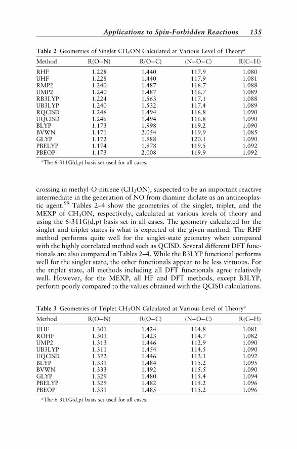
crossing in methyl-O-nitrene (CH3ON), suspected to be an important reactiveintermediate in the generation of NO from diamine diolate as an antineoplas-tic agent.99 Tables 2–4 show the geometries of the singlet, triplet, and theMEXP of CH3ON, respectively, calculated at various levels of theory andusing the 6-311G(d,p) basis set in all cases. The geometry calculated for thesinglet and triplet states is what is expected of the given method. The RHFmethod performs quite well for the singlet-state geometry when comparedwith the highly correlated method such as QCISD. Several different DFT func-tionals are also compared in Tables 2–4. While the B3LYP functional performswell for the singlet state, the other functionals appear to be less virtuous. Forthe triplet state, all methods including all DFT functionals agree relativelywell. However, for the MEXP, all HF and DFT methods, except B3LYP,perform poorly compared to the values obtained with the QCISD calculations.

Table 2 Geometries of Singlet CH3ON Calculated at Various Level of Theorya

Method R(O��N) R(O��C) (N��O��C) R(C��H)

RHF 1.228 1.440 117.9 1.080UHF 1.228 1.440 117.9 1.081RMP2 1.240 1.487 116.7 1.088UMP2 1.240 1.487 116.7 1.089RB3LYP 1.224 1.563 117.1 1.088UB3LYP 1.240 1.532 117.4 1.089RQCISD 1.246 1.494 116.8 1.090UQCISD 1.246 1.494 116.8 1.090BLYP 1.173 1.998 119.2 1.090BVWN 1.171 2.054 119.9 1.085GLYP 1.172 1.988 120.1 1.090PBELYP 1.174 1.978 119.5 1.092PBEOP 1.173 2.008 119.9 1.092

aThe 6-311G(d,p) basis set used for all cases.

Table 3 Geometries of Triplet CH3ON Calculated at Various Level of Theorya


UHF 1.301 1.424 114.8 1.081ROHF 1.303 1.423 114.7 1.082UMP2 1.313 1.446 112.9 1.090UB3LYP 1.311 1.454 114.5 1.090UQCISD 1.322 1.446 113.1 1.092BLYP 1.331 1.484 115.2 1.095BVWN 1.333 1.492 115.5 1.090GLYP 1.329 1.480 115.4 1.094PBELYP 1.329 1.482 115.2 1.096PBEOP 1.331 1.485 115.2 1.096



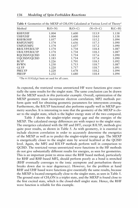
As expected, the restricted versus unrestricted HF wave functions give essen-tially the same results for the singlet state. The same conclusion can be drawnfor the MEXP search in this particular example. Overall, optimization of theMEXP geometry must incorporate electron correlation; MP2 methods per-form quite well for obtaining geometric parameters for intersystem crossing.Furthermore, the B3LYP functional also performs equally well in MEXP geo-metry searches. It is interesting to note that the geometry of the MEXP is clo-ser to the singlet state, which is the higher energy state of the two compared.

Table 5 shows the singlet–triplet energy gap and the energies of theMEXP. The calculated energy differences are with respect to the singlet state.The energetics calculated with the HF and DFT, except B3LYP, methods givequite poor results, as shown in Table 5. As with geometry, it is essential toinclude electron correlation in order to accurately determine the energeticsof the MEXP as well as to predict the singlet–triplet energy gap. The MEXPis energetically closer to the singlet state by several kcal/mol at the QCISDlevel. Again, the MP2 and B3LYP methods perform well in comparison toQCISD. The restricted versus unrestricted wave functions in the HF methodsdo not give substantially different results for energies, as seen for geometries.This is an important point to stress since the RHF based method, particularlyfor RHF and RHF-based MP2, should perform poorly as a bond is stretched(RHF eventually converges to the ionic asymptote and perturbation theorybreaks down due to near degeneracy). However, for the problem at handRHF and UHF based wave functions give essentially the same results, becausethe MEXP is located energetically close to the singlet state, as seen in Table 5.The ground state of CH3ON is a triplet state, and the MEXP is found close tothe first excited state, which is the closed-shell singlet state. Hence, the RHFwave function is reliable for this example.

Table 4 Geometries of the MEXP of CH3ON Calculated at Various Level of Theorya


RHF/UHF 1.004 1.600 113.9 1.138UHF/UHF 1.004 1.600 114.0 1.138RHF/ROHF 1.057 1.698 115.2 1.094RMP2/UMP2 1.174 1.656 117.3 1.090UMP2/UMP2 1.174 1.657 117.2 1.090RB3LYP/UB3LYP 1.174 1.734 118.4 1.087UB3LYP/UB3LYP 1.174 1.734 118.3 1.087RQCISD/UQCISD 1.183 1.714 117.6 1.090UQCISD/UQCISD 1.183 1.714 117.6 1.090BLYP 1.226 1.701 118.5 1.092BVWN 1.230 1.713 118.7 1.087GLYP 1.220 1.717 118.7 1.091PBELYP 1.228 1.678 118.2 1.094PBEOP 1.232 1.680 118.4 1.094



For larger polyatomic molecules, many more degrees of freedom existgiving rise to flexibility in crossing. In comparing HON and C6H5��ON, inwhich the ground states are the triplet states, �ES-T¼�21.8 and �17.4kcal/mol, respectively. The MEXP lies 11.8 and 1.1 kcal/mol higher thanthe corresponding singlet states at the MP2/6-311G(d,p) level of theory (thezeroth-order functions are RHF for singlet and UHF for triplet). These resultsindicate that the higher the number of degrees of freedom the closer in energythe MEXP is to the higher energy of the two states in question. Therefore, theeffective barrier toward spin-forbidden reaction is lower in larger polyatomicmolecules resulting in facile intersystem crossing.

Phenyl Cation

Intersystem crossing in the phenyl cation was examined by Harveyet al.75 The aforementioned hybrid method utilizing Eqs. [98] and [99] wasused to locate the MEXP between singlet and triplet states at various levelsof theory with the 6-31G(d) basis set. A comparison was made betweenHF//HF, B3LYP//HF, B3LYP//B3LYP B3LYP//HF, and CCSD(T)//B3LYP,where the double-slashes delineate the higher level (energy calculation) andlower level (gradient calculation) in the hybrid method. The singlet state ofthe phenyl cation is the ground state, and the triplet state lies 19 kcal/mol

Table 5 Singlet–Triplet Energy Gap and Energies ofthe MEXP of CH3ONa

Method �ES�T �EMEXP

RHF/UHF �39.1 80.6UHF/UHF �39.1 80.6RHF/ROHF �32.9 80.6RMP2/UMP2 �15.4 4.4UMP2/UMP2 �15.4 4.4RB3LYP/UB3LYP �16.6 �0.8UB3LYP/UB3LYP �16.0 1.5RQCISD/UQCISD �16.5 3.4UQCISD/UQCISD �16.5 3.4BLYP �5.4 2.4BVWN �3.9 3.3GLYP �6.6 2.1PBELYP �4.6 2.6PBEOP �3.8 3.1

aThe methods used for calculations are denoted as ‘‘A/B’’,where A is for the singlet state and B for the triplet state. Forthe DFT functionals, BLYP to PBEOP (last five rows) only therestricted calculations for the singlet and unrestricted calcula-tions for the triplet states were performed. The calculatedenergetics is with respect to respective singlet state energies. Allcalculations were performed with the 6-311G(d,p) basis set.


above the singlet using the CCSD(T)/6-31G(d) energy at the B3LYP/6-31G(d)optimized geometry. By using the CCSD(T)//B3LYP method, the MEXP wasfound to be only 0.2 kcal/mol above the triplet state. If B3LYP/6-31G(d) isused for the optimization, the singlet–triplet energy gap is 16.4 and theMEXP is 0.3 kcal/mol above the triplet state. The geometry of the MEXP cal-culated with the correlated systems (including B3LYP) is close to that of thetriplet-state geometry. The authors also calculated the spin–orbit couplingmatrix elements using the Zeff method and obtained 8 cm�1. Even with thespin–orbit interaction being small, the triplet state should undergo very effi-cient intersystem crossing due to its closeness to the MEXP geometry.

Norbornene

The triplet state of ethylene assumes a twisted conformation, and has arelatively short lifetime. The triplet state of norbornene also has a short life-time, even though the twisted configuration cannot be achieved due to its rigidframework.100 The short lifetime of triplet norbornene has been investigatedby Harvey et al.101 Their calculations were carried out at the unrestrictedB3LYP/SVþ d level of theory by varying the dihedral angle around the pbond. The dihedral angle must become 98� for the singlet surface to crossthe triplet state, and this point of crossing is 15 kcal/mol above the triplet mini-mum. From a one-dimensional dihedral coordinate, the anharmonic vibra-tional Schrodinger equation was solved in order to obtain the Franck–Condon overlap for a golden rule calculation (Eq. [5]). The rest of the vibra-tional degrees of freedom were treated as unity, being considered as the bathmodes. In conjunction with spin–orbit coupling matrix elements calculated byusing the method of Koseki et al.,7,8 Harvey et al.101 were able to calculate theintersystem crossing rate to be 3:4� 108 s�1, which corresponds to a 3-ns life-time. This result underestimates the experimental lifetime of 250 ns. Theyfurther calculated the MEXP using Eqs. [98] and [99], and found that a tripletminimum is 67 kcal/mol above the singlet state and that the optimized MEXPwith dihedral angles >90� lies 8 kcal/mol above the triplet state. These resultswere based on utilizing two-electron two-orbital CASSCF/SVþ d level oftheory. Using their nonadiabatic RRKM theory20 with an Airy function pre-dicts a crossing rate of 3� 105 s�1, which corresponds to a 3000-ns lifetime,giving better agreement with the experimental lifetime.

Conjugated Polymers

Poly(phenylenevinylene) has been considered for many different applica-tions due to its importance in nanoscale electronic devices. One such applica-tion is the search for efficient light emitting diodes. This property is the resultof the electrooptical effect and constitutes an important area of modernresearch in theory as well as experiment. The efficiency of the nonradiative


decay path, particularly of singlet–triplet intersystem crossing, can lowerdevice efficiency. Beljonne et al.102 examined the intersystem crossing in oli-go(phenylene ethylene) and oligothiophenes with differing polymeric lengthwithin a framework of semiempirical INDO/CIS. The spin–orbit couplingwas calculated from the one-electron Breit–Paui Hamiltonian using first-orderperturbation theory and was used for subsequent calculation of the intersys-tem crossing rate through the Fermi golden rule. The singlet–triplet energygaps, S0 � T1 decreases as the chain becomes longer, as expected from bandtheory. Hence, intersystem crossing becomes more efficient.

CHð2�Þ þN2 ! HCNþNð4SÞThere have been a number of theoretical investigations on the

CHþN2! HCNþN system due, in part, to its importance in the produc-tion of NO in the combustion chemistry of hydrocarbons. It is also interestingfrom the perspective of electronic structure theory because it involves potentialenergy surfaces of the doublet and quartet states and spin–orbit coupling con-necting these states, and because aspects of dynamics by a generalized transi-tion state theory and a nonadiabatic RRKM theory can be used.

Manaa and Yarkony73b investigated the stationary points on the relevantpart of the potential energy surfaces by using second-order configuration inter-action based on SA–MCSCF wave functions. One of the two crossing pointsfound for the study is that of a higher energy, colinear structure where the Natom is coordinated to NCH in C1v symmetry. It was suggested that thecolinear structure is not involved in the reaction because of its high barrier(50 kcal/mol) with respect to the HCNþN(4S) asymptote. The lower energycrossing point has an approximately C2v structure with HC bifurcating thetwo nitrogen atoms. This structure is � 7 kcal/mol above the HCNþN(4S)asymptote. Spin–orbit coupling between doublet and quartet states was calcu-lated at the C2v MEXP, using the full Breit–Pauli Hamiltonian based on SA–MCSCF/CI (second-order) wave functions, and was found to be 11 cm�1. Onthe basis of their spin–orbit coupling, Manaa and Yarkony also estimated thetransition probability from the doublet to the quartet by using the Landau–Zener model. They found the crossing probability to be in the range of1:5� 10�3–5� 10�4, which translates to the same order of magnitudeobtained for a reasonable Arrhenius A factor. Later, Cui and Morokumaobtained a similar potential energy surface for the reaction, including thetwo minimum energy crossing points.103 Based on the points of the potentialenergy surface calculated by Manaa and Yarkony, Seideman and Walch104

constructed a two-dimensional surface for doublet and quartet states. Subse-quently, Seideman105 computed the energy-dependent reaction probability byutilizing the discrete variable representation106 with absorbing boundaryconditions (ABC–DVR).95 The energy-dependent reaction probability wascalculated in terms of two unimolecular decay probabilities and of the


doublet–quartet hopping probability evaluated within the golden rule usingspin–orbit coupling data based on Manaa and Yarkony. The calculatedenergy-dependent reaction probability shows resonance features giving riseto several high reaction probability peaks within the energy range examined.Furthermore, the cumulative reaction probability is averaged over the energydistribution to obtain the thermal rate constant. The calculated thermal rateconstant shows qualitative agreement with the available experimental rateconstant. Cui et al. derived an expression for cumulative reaction probabilityfor the reaction by extension of the united statistical theory, consideringthe minimum energy crossing point treated as a transition state, and obtainedqualitative agreement with experimental results.107

Molecular Properties

As mentioned above, the ESR spectrum is affected by the strength ofspin–orbit coupling in molecules. The effect of spin–orbit coupling in ESR isrepresented by the Hamiltonian, H ¼ mB SgB, where mB is the Bohr magneton,S is spin, g is the so-called g-tensor, and B is the external magnetic field. For afree electron g¼ 2.0023. The shift in g due to the molecular environment andto the external magnetic field was calculated by Engstrom et al.108 from theproduct of spin–orbit and orbital Zeeman matrix elements ½h�0jHSOj�nih�njLj�0i�=ðE0 � EnÞ with perturbation theory. The authors examined theg-tensor of a spin-label nitroxide with two hydrogen-bonded configurationsby using ROHF linear response theory and the atomic mean-field approxima-tion for spin–orbit coupling. They showed that much of the spin density islocated at the N and O atoms of the nitroxide group and if the hydrogenbond is directly bonded to the nitroxide center, the spin–orbit couplingdecreases. Hence, one of the components of the g-tensor decreases in agree-ment with the experiments. Similar studies of the g-tensor were carried out,where the atomic mean-field approximation was compared with the fullBreit–Pauli results on molecules such as CH3, SiH3, GeH3, ClO2, ClSO,SlS2, benzene cation, benzene anion, and other molecules.109

Due to its tremendous usefulness in many subdisciplines of the chemicalsciences, calculations of the (NMR) shielding constant110 have become animportant area of research. The NMR shielding constant is given as a sumof four contributions: diamagnetic, paramagnetic, spin-dipolar, and Fermicontact terms. All terms are affected by spin–orbit coupling, but particularlythe Fermi contact term becomes important when heavy atoms are involved.Nakatsuji et al.111 obtained results based on finite perturbation theory usingUHF wave functions. Their method was applied to SnX4, where X¼H, Cl,Br, and I as well as to SnBr4-nIn (n ¼ 1, 2, 3) showing the importance of thespin–orbit contribution to the shielding constant.112 The authors further foundthat the large spin–orbit coupling contribution is due to the Fermi contactterm. Similar work utilizing density functional theory with the mean-field


spin–orbit method was done by Malkina et al.113 who compared the shieldingsof CH3X, where X¼ F, Cl, Br, and I. Similar DFT work on the secondaryisotope shifts in CX2, where X¼O, S, Se, and Te has also been carried out.114

Dynamical Aspects

Nakajima and Kato examined115 the collision induced intersystem cros-sing in the excited state of the Ar–glyoxal system. By using CASSCF on the rele-vant part of the potential energy surfaces of the first excited S1 and T1 states,the potentials were fitted to analytical functions. The spin–orbit matrix wascalculated by using the Breit–Pauli Hamiltonian at each geometry. The quan-tum mechanical dynamics were carried out by time-propagating the probabil-ity amplitude of the vibrational degrees of freedom. The dynamics werecarried out in two ways; one was done perturbatively, and the other wasdone by introducing the level shift as a parameter. From their electronic struc-ture and dynamics calculations, it was shown that the intermolecular spin–orbit coupling is induced by an Ar atom approaching glyoxal. This approachis due to p-interaction. The Ar atom must approach glyoxal from a directionother than its molecular plane because the coplanar approach by Ar gives zerospin–orbit interaction. Also, it was found that the intermolecular spin–orbitcoupling increases the transition cross section by >100 times the cross-sectionobtained by the intramolecular spin–orbit interaction alone.

Another aspect of dynamics was evaluated by Niv, Bargheer, and Gerberwho studied the photodissociation dynamics of F2 in an Ar54 cluser.116 Mod-eling condensed-phase reaction dynamics is difficult due to many-body inter-actions. However, a model with an inert medium is a convenient way toexamine the role that a medium can play in the condensed phase. Becausethe system is large and a full quantum mechanical description of the dynamicsis computationally prohibitive, the authors used the semiclassical surface hop-ping method117 to carry out the dynamics simulations. The states of F2, corre-sponding to a gas-phase equivalent, included in the condensed-phase study aretwo 1�g, one 1�u, two 1�g, two 1�u, two 1�g, two 3�u, two 3�g, two 3�u, one3�g, and two 3�g, giving nine singlet and 27 (3� 9) triplet states. The empiri-cal potential of Aquilanti et al.118 as well as an ab initio potential calculated atthe CCSD(T)/aug-cc-pVTZ level of theory were used for this study. The disso-ciating F atoms collide with a cage of Ar atoms and transfer most of theirkinetic energy, within � 100 fs, causing evaporation of Ar atoms in the outer-most layer. The results of their surface hopping trajectory calculations alsoindicate that substantial recombination occurs � 100 fs after photoexcitation.The F2 molecule is initally in its 1�u state, but becomes trapped in its 3�u state,which oscillates about 4 bohr. They found two types of dissociative processes;one is the direct dissociation and the other involves cage-oscillation first, fol-lowed by dissociation. Direct dissociation takes place within 200 fs. In the caseof delayed dissociation, an F atom leaves the cage after two oscillations (first


oscillation takes place within 100 fs with smaller amplitude, and the secondoscillation takes place within 700 fs). The average of all triplet-state popula-tions is markedly different from the simulated recombination effect for the 3�u

state. This unusually high population of the 3�u state is due to the fact that thespin–orbit coupling directly couples the initially prepared state (1�u) tothe 3�u state. Observation of such an effect has been confirmed recently byfemtosecond pump–probe experiments.119 A similar dynamics study has alsobeen carried out by Krylov et al. on Cl atom relaxation in solid Ar.120

Daniel et al.121 examined photodissociation dynamics involving intersys-tem crossing in HCo(CO)4. They used the Chebychev propagator94 for solvingthe time-dependent Schrodinger equation using one- and two-dimensionalpotential energy surfaces generated by the CASSCF/CI method. They observedthat 35% of the product is the singlet primary product occurring within 20 fs.The triplet channels in comparison are relatively slow, but accessible within50 ps. They concluded that intersystem crossing is on the same time scale asintramolecular vibrational relaxation and it is competitive to indirect dissocia-tion induced by tunneling in this system.

OTHER REACTIONS

An asymmetric nitric oxide dimer N��N��O��O (a-N2O2) has been exam-ined as a possible energetic material. The a-N2O2 (1A0 ground state) is calcu-lated to be 102 and 62 kcal/mol higher with respect to N2þO2 and NOþNOasymptotes, respectively.122 Nguyen et al.,123 examined a possible spin-forbidden decay path of a-N2O2. They used Eq. [92] to obtain the MEXPbetween 1A0 and 3A00 states based on the a-N2O2 (1A0)! N2O2

(3A00)! N2O (X1�þ) þ O (3P) reaction. To do this, they used SA–MCSCF/SOCI along with DZP and TZP basis sets, in addition to full Breit–Paulispin–orbit matrix elements. They found that the intersystem crossing of a-N2O2 is efficient, since the MEXP between 1A0 and 3A00 is only 1–2 kcal/mol above the singlet state and the calculated spin–orbit coupling is relativelylarge (75 cm�1).

Using a Fourier transform ion cyclotron resonance (FT–ICR) spectro-meter, Janaway and Brauman124 examined the proton-transfer reaction for3NO� þH2S! 1HNOþHS�. The reaction is exothermic by 12 kcal/mol,and the triplet complex 3NO��H2S and singlet complex 1NO��H2S are 18and 23 kcal/mol below reactants, respectively. The minimum energy crossingpoint is located 2 kcal/mol above the triplet complex suggesting that the reac-tion should be efficient energetically. However, the reaction is not observedexperimentally. Interestingly, 3NO� reacts with relatively high efficiencywith (CH3)3CSH, which the authors speculated arises from similar kineticsas for the curve crossing found in H2S. Their RRKM calculations on the


dissociation rate of the triplet complex to reactants show that the rate differsby three orders of magnitude slower for the (CH3)3CSH, due to denservibrational manifolds, than for H2S. Therefore, the (CH3)3CSH complexhas more chance to undergo a spin-forbidden transition than the H2S complexhas.

In another study, Mebel et al.125 examined the photodissociation pathinvolving a spin-forbidden channel in methane. Their MRCI and equationof motion (EOM) CCSD calculations, including MEXP, indicated that thephotodissociation pathway is likely to proceed via intersystem crossing fromS1(1A’’) to repulsive T1(3A’), instead of the speculated S0 S1 internal conver-sion. Similar studies have been done by Hwang and Mebel on spin-forbiddenreactions in N2O! N2þO (3P) and N2O! N2þO (1D).126

Other reactions of spin-forbidden processes include a study by Mannaand Chabalowski127 on the reaction, NO (X2�)þCO (X1�þ)! N(4S)þCO2 (X1�þg ), using the SA–MCSCF/SOCI approach to locate theMEXP (60 kcal/mol above the reactants). A similar study was carried out128

on CH3 (X2A2’’)þN(4S)! HCN (X1�þ)þH2 (X1�þg ), where it was foundthat the MEXP is located below (8 kcal/mol) the reactants. The barrierlesstransition occurs at the MEXP in 1 out of 208 vibrational periods, as deducedfrom the Landau–Zener transition probability using a 30 cm�1 spin–orbitmatrix element.

Finally, Veige et al.129 examined singlet- and triplet-state energies as wellas MEXP for M(OH)3, where M¼V, Nb, and Ta, in connection with thedeoxygenation process of (silox)3WNO by M(OR)3. They found M(OH)3 isa triplet ground state for M¼V, singlet for M¼ Ta, and almost isoenergeticfor M¼Nb. The MEXP, calculated at the B3LYP/SBKJC40 level, were foundto be 1–2 kcal/mol above the higher states of the two examined for M(OH)3.

BIOLOGICAL CHEMISTRY

One area of research that has not been explored very much by the tech-niques covered in this chapter is biological chemistry. Many enzymes carry outelectron-transfer reactions, and can undergo intersystem crossing.130 Manyof the methodologies discussed in this chapter are applicable to biologicalsystems exhibiting spin-forbidden transitions.

Since the ground state of oxygen is a triplet state (X3�g�), it is reason-able to assume that spin-forbidden reactions should take place at some stepin a sequence of reactions that leads eventually to a singlet product. Flavinadenine dinucleotide (FAD) is a cofactor in enzymes, and is the redox centerfor transferring electrons to and from substrates.131 Molecular oxygen is oneof the substrates that FAD-containing enzymes catalyze to produce H2O2.Therefore, the overall reaction is spin-forbidden.

Biological Chemistry 143

A study by Prabhakar et al.,132 examined the reaction mechanism ofthe peroxidation process for glucose oxidase by modeling the active site ofthe enzyme including FADH2 (reduced form of FAD) and a histidine residueresponsible for binding and subsequent transfer of hydrogen atom to molecu-lar oxygen. Their calculations involved full geometry optimization, using theB3LYP/DZ(d,p) and B3LYP/6-311þG(2d,2p) levels of theory; unrestrictedwave functions were used for the triplet state. The peroxidation process,O2þ FADH2! H2O2þ FAD, was found to occur via electron trasfer fromFADH2 forming a triplet radical pair, subsequent intersystem crossing to thesinglet state (open-shell singlet radical), where the minimum geometries of thetriplet and open-shell singlet are nearly equal. They concluded that intersystemcrossing is barrierless. Subsequently, a proton is transferred from the proto-nated histidine residue to form hydrogen peroxide and the authors found atransition state for such a process, showing the existence of a deuteriumisotope effect in the second step, even though no such effect is found experi-mentally. Instead, an oxygen isotope effect is found experimentally. This leadsto the conclusion that the rate-limiting step is the first intersystem crossingreaction step. The spin–orbit matrix element between open-shell singlet andtriplet was estimated to be 76.5 cm�1 from a model system. In terms of theFermi golden rule, the authors discussed how the rate of transition dependson the spin–orbit coupling of the system.

CONCLUDING REMARKS

Models related to spin-forbidden reactions are discussed in this chapter.Coupling between two surfaces of different spin and symmetry is given byvarious levels of approximation for spin–orbit operators from the reductionof relativistic quantum mechanics. Well-established methods such as theBreit–Pauli Hamiltonian exist, but new relativistic methods such as theDouglas–Kroll Hamiltonian and other new transformation schemes are alsobeing investigated and implemented today.

Locating crossing points between the two surfaces gives an effective bar-rier in spin-forbidden reactions. Particularly important is the MEXP and algo-rithms to locate it. A wide range of theoretical methods are available forexamining different aspects of spin-forbidden reaction dynamics, rangingfrom Fermi’s golden rule to quantum dynamics by solving the time-dependentSchrodinger equation. Currently, applications in the literature are limited torelatively small molecules. Applications to areas such as biological chemistryand transition metal catalysis are not currently explored by these methods;however, many such systems contain aspects of spin-forbidden reactionsthat need to be investigated computationally to give meaningful explanationsof the observed phenomena.


ACKNOWLEDGMENTS

NM wishes to thank Prof. T. R. Cundari for a long-standing collaboration and on-goingcommunications; he also acknowledges encouragement and stimulating discussions with his col-leagues Professor Andreas A. Zavitsas, Professor Don W. Rogers, and Professor Frank McLaffertyof LIU.

REFERENCES

1. The nonadiabatic coupling matrix element is a consequence of the Born–Oppenheimerapproximation, as shown in texts such as: (a) F. Jensen, Introduction to ComputationalChemistry, Wiley, West Sussex, England, Chapter 3, p. 53. Further details on thenonadiabatic coupling matrix elements can be found in (b) D. R. Yarkony, ModernElectronic Structure Theory, D. R. Yarkony, Ed., World Scientific, Singapore, 1995, Part1, Chapter 11, p. 642. Electronic Structure Aspects of Nonadiabatic Processes in PolyatomicSystems.

2. (a) K. Fukui, Acc. Chem. Res., 14, 363 (1981). The Path of Chemical Reactions—The ICRApproach. b) H. B. Schlegel, in Modern Electronic Structure Theory, D. R. Yarkony, Ed.,World Scientific, Singapore, 1995, Part 1, Chapter 8, p. 459. Geometry Optimization onPotential Energy Surfaces.

3. N. Lehnert, R. Y. N. Ho, L. Que, and E. I. Solomon, J. Am. Chem. Soc., 123, 8271 (2001).Spectroscopic Properties and Electronic Structure of Low-Spin Fe(III)-Alkylperoxo Com-plexes: Homolytic Cleavage of the O��O Bond.

4. J. N. Harvey, in Computational Organometallic Chemistry, Thomas R. Cundari, Ed., MarcelDekker, New York, 2001, p. 291. Spin-Forbidden Reactions in Transition-Metal Chemistry.

5. S. Kato, R. L. Jaffe, A. Komornicki, and K. Morokuma, J. Chem. Phys., 78, 4567 (1983). ATheoretical Study on the Mechanism of Electronic to Vibrational Energy Transfer inHg(3P)þCO Collisions.

6. (a) P. Pyykko and J. Desclaux, Acc. Chem. Res., 12, 276 (1979). Relativity and the PeriodicSystem of Elements. (b) P. Pyykko, Chem. Rev., 88, 563 (1988). Relativiestic Effects inStructural Chemistry. (c) K. S. Pitzer, Acc. Chem. Res., 12, 271 (1979). Relativistic Effects onChemical Properties. (d) W. Kutzelnigg, Physica Scripta, 36, 416 (1987). The RelativisticMany Body Problem in Molecular Theory.

7. S. Koseki, M. S. Gordon, M. W. Schmidt, and N. Matsunaga, J. Phys. Chem., 99, 12764(1995). Main Group Effective Nuclear Charges for Spin–Orbit Calculations.

8. S. Koseki, M. W. Schmidt, and M. S. Gordon, J. Phys. Chem. A, 102, 10430 (1998). EffectiveNuclear Charges for the First- Through Third-Row Transition Metal Elements in Spin–OrbitCalculations.

9. S. Koseki, D. G. Fedorov, M. W. Schmidt, and M. S. Gordon, J. Phys. Chem. A, 105, 8262(2001). Spin–Orbit Splittings in the Third-Row Transition Elements: Comparison ofEffective Nuclear Charge and Full Breit–Pauli Calculations.

10. NIST atomic spectra database. http://physics.nist.gov/cgi-bin/AtData/main_asd

11. W. J. Stevens and M. Krauss, Chem. Phys. Lett., 86, 320 (1982). Ab Initio Effective Spin–Orbit Operators for Use in Atomic and Molecular Structure Calculations. Results for Carbonand Silicon.

12. N. J. Turro, Modern Molecular Photochemistry, Chapter 8, University Science Books,Sausalito, California (1991). ESR.

13. I. V. Khudyakov, Y. A. Serebrennikov, and N. J. Turro, Chem. Rev., 93, 537 (1993). Spin–Orbit Coupling in Free-Radical Reactions: On the Way to Heavy Elements.

14. N. Matsunaga, D. W. Rogers, and A. A. Zavitsas, J. Org. Chem., 68, 3158 (2003). Pauling’sElectronegativity Equation and a New Corollary Accurately Predict Bond DissociationEnthalpies and Enhance Current Understanding of the Nature of the Chemical Bond.

References 145

15. S. Yabushita, J. Mol. Struct. (THEOCHEM), 461–462, 523 (1999). Potential Energy Curvesof ICl and Non-Adiabatic Interactions Studied by the Spin–Orbit CI Method.

16. H. J. Silverstone and O. Sinanoglu, J. Chem. Phys., 44, 1899 (1966). Many-Electron Theory ofNonclosed-Shell Atoms and Molecules. I. Orbital Wavefunction and Perturbation Theory.

17. N. Matsunaga, S. Koseki, and M. S. Gordon, J. Chem. Phys., 104, 7988 (1996). RelativisticPotential Energy Surfaces of XH2 (X¼C, Si, Ge, Sn, and Pb) Molecules: Coupling of 1A1 and3B1 States.

18. J. C. Tully, J. Chem. Phys., 61, 61 (1974). Collision Complex Model for Spin ForbiddenReactions: Quenching of O(1D) by N2.

19. T. Seideman, J. Chem. Phys., 101, 3662 (1994). Resonances in the CHþN2! HCNþN(4S)Reaction: The Dynamics of a Spin-Forbidden Process.

20. (a) J. C. Lorquet and B. Leyh-Nihant, J. Phys. Chem., 92, 4778 (1988). NonadiabaticUnimolecular Reactions. 1. A Statistical Formulation for the Rate Constants. (b) F. Remacle,D. Dehareng, and J. C. Lorquet, J. Phys. Chem., 92, 4784 (1988). Nonadiabatic Unim-olecular Reactions. 2. Isotope Effects on the Kinetic Energy Release.

21. M. S. Child, Molecular Collision Theory, Dover, Mineola, New York, 1976.

22. C. Zhu, Y. Teranishi, and H. Nakamura, Adv. Chem. Phys., 117, 127 (2001). NonadiabaticTransitions Due to Curve Crossings: Complete Solutions of the Landau–Zener–StueckelbergProblems and Their Applications.

23. H. Nakamura, Nonadiabatic Transition, Concepts, Basic Theories, and Applications, WorldScientific, Singapore, 2002.

24. J. Almlof and O. Gropen, in Reviews in Computational Chemistry, K. B. Lipkowitz and D. B.Boyd, Eds., VCH Publishers, Weinheim, Germany (1996), pp. 203–244. Relativistic Effectsin Chemistry.

25. B. A. Hess, C. M. Marian, and S. D. Peyerimhoff, in Modern Electronic Structure Theory, Part1, D. R. Yarkony, Ed., World Scientific, Singapore, 1995, p. 152. Ab Initio Calculation ofSpin–Orbit Effects in Molecules Including Electron Correlation.

26. (a) W. Greiner, Relativistic Quantum Mechanics, Wave Equations, Springer-Verlag, Berlin,1990. (b) A. Messiah, Quantum Mechanics, Dover Publications, Inc., Mineola, New York,1999.

27. See, for example, (a) L. Pisani and E. Clementi, J. Comput. Chem., 15, 466 (1994). RelativisticDirac–Fock Calculations for Closed-Shell Molecules. (b) Relativistic Effects in Heavy-Element Chemistry and Physics, B. A. Hess, Ed., Wiley, West Sussex, England, 2003.

28. J. P. Desclaux, Computer Phys. Comm., 9, 31 (1975). A Multiconfiguration RelativisticDirac–Fock Program.

29. (a) A. J. Sadlej, in Lecture Notes in Chemistry, 64, Lecture Notes in Quantum Chemistry:European Summer School in Quantum Chemistry, B. O. Roos, Ed., Springer-Verlag, Berlin(1994) p. 203. Methods of Relativistic Quantum Chemistry. (b) J. Sucher, Phys. Rev. A, 22,348 (1980). Foundations of the Relativistic Theory of Many-Electron Atoms. (c) O. Visser,L. Visscher, P. J. C. Aerts, and W. C. Nieuwpoort, Theor. Chim. Acta, 81, 405 (1992).Relativistic All-Electron Molecular Hartree–Fock–Dirac–(Breit) Calculations on CH4, SiH4,GeH4, SnH4, PbH4. (d) E. Eliav and U. Kaldor, Chem. Phys. Lett., 248, 405 (1996). TheRelativistic Four-Component Coupled Cluster Method for Molecules: Spectroscopic Con-stants of SnH4. (e) E. Eliav, U. Kaldor, and Y. Ishikawa, Phys. Rev. A, 49, 1724 (1994).Open-Shell Relativistic Coupled-Cluster Method with Dirac–Fock–Breit Wave Functions:Energies of the Gold Atom and Its Cation.

30. G. Breit, Phys. Rev., 34, 553 (1929). The Effect of Retardation on the Interaction of TwoElectrons.

31. K. G. Dyall, J. Chem. Phys., 100, 2118 (1994). An Exact Separation of the Spin-Free andSpin-Dependent Terms of the Dirac–Coulomb–Breit Hamiltonian.

32. L. L. Foldy and S. A. Wouthuysen, Phys. Rev., 78, 29 (1950). On the Dirac Theory of Spin 12

Particles and Its Nonrelativistic Limit.


33. S. R. Langhoff and C. W. Kern, in Modern Theoretical Chemistry, H. F. Schaefer III, Ed.,Vol. 4. Plenum Press, New York, p. 381. Chapter 10. Molecular Fine Structure.

34. D. R. Yarkony, Int. Rev. Phys. Chem., 11, 195 (1992). Spin-Forbidden Chemistry within theBreit–Pauli Approximation.

35. H. A. Bethe and E. E. Salpeter, Quantum Mechanics of One- and Two-electron Atoms,Springer-Verlag, Berlin, 1957, p. 170.

36. (a) T. R. Furlani and H. F. King, J. Chem. Phys., 82, 5577 (1985). Theory of Spin–OrbitCoupling. Application to Singlet–Triplet Interaction in the Trimethylene Biradical. (b) T. R.Furlani, Ph. D. dissertation, State University of New York, Buffallo, 1984.

37. D. G. Fedorov and M. S. Gordon, J. Chem. Phys., 112, 5611 (2000). A Study of the RelativeImportance of One and Two-Electron Contributions in Spin–Orbit Coupling.

38. W. R. Wadt, Chem. Phys. Lett., 89, 245 (1982). An Approximate Method to IncorporateSpin–Orbit Effects into Calculations Using Effective Potentials.

39. S. Koseki, M. W. Schmidt, and M. S. Gordon, J. Phys. Chem., 96, 10768 (1992). MCSCF/6-31G(d,p) Calculations of One-Electron Spin–Orbit Coupling Constants in DiatomicMolecules.

40. (a) W. J. Stevens, H. Basch, and M. Krauss, J. Chem. Phys. 81, 6026 (1984). CompactEffective Potentials and Efficient Shared-Exponent Basis Sets for the First- and Second-Row Atoms. (b) W. J. Stevens, H. Basch, M. Krauss, and P. G. Jasien, Can. J. Chem, 70,612 (1992). Relativistic Compact Effective Potentials and Efficient, Shared-ExponentBasis Sets for the Third-, Fourth-, and Fifth-Row Atoms. (c) T. R. Cundari and W. J.Stevens, J. Chem. Phys., 98, 5555 (1993). Effective Core Potential Methods for theLanthanides.

41. K. P. Huber and G. Herzberg, Constants of Diatomic Molecules (data prepared by J.W.Gallagher and R.D. Johnson, III), in NIST Chemistry WebBook, NIST Standard ReferenceDatabase Number 69, P. J. Linstrom and W. G. Mallard, Eds., March 2003, NationalInstitute of Standards and Technology, Gaithersburg MD, 20899 (http://webbook.nist.gov).

42. T. R. Cundari, M. T. Benson, M. L. Lutz, and S. O. Sommerer, in Reviews in ComputationalChemistry, Vol. 8, K. B. Lipkowitz and D. B. Boyd, Eds., VCH Publishers, Weinheim,Germany, 1996, p. 145. Effective Core Potential Approaches to the Chemistry of the HeavierElements.

43. G. Fenking, I. Antes, M. Bohme, S. Dapprich, A. W. Ehlers, V. Jonas, A. Neuhaus, M. Otto,R. Stegmann, A. Veldkamp, and S. F. Vyboishchikov, in Reviews in ComputationalChemistry, Vol. 8, K. B. Lipkowitz and D. B. Boyd, Eds., VCH Publishers, Weinheim,Germany, 1996, p. 63. Pseudopotential Calculations of Transition Metal Compounds: Scopeand Limitations.

44. M. Krauss and W. J. Stevens, Annu. Rev. Phys. Chem., 35, 357 (1984). Effective Potentials inMolecular Quantum Chemistry.

45. W. C. Ermler, Y. S. Lee, P. A. Christiansen, and K. S. Pitzer, Chem. Phys. Lett., 81, 70 (1981).Ab Initio Effective Core Potentials Including Relativistic Effects. A Procedure for theInclusion of Spin–Orbit Coupling.

46. (a) P. A. Christiansen, W. C. Ermler, and K. S. Pitzer, Annu. Rev. Phys. Chem., 36, 407 (1985).Relativistic Effects in Chemical Systems. (b) W. C. Ermler, R. B. Ross, and P. A. Christiansen,Adv. Quantum Chem., J. R. Sabin and M. C. Zerner, Eds., Academic Press, SanDiego, CA, 1988, p.139. Spin–Orbit Coupling and Other Relativistic Effecs in Atomsand Molecules.

47. L. F. Pacios and P. A. Christiansen, J. Chem. Phys., 82, 2664 (1985). Ab Initio RelativisticEffective Potentials with Spin–Orbit Operators. I. Li through Ar.

48. M. M. Murley, L. F. Pacios, P. A. Christiansen, R. B. Ross, and W. C. Ermler, J. Chem. Phys.,84, 6840 (1986). Ab Initio Relativistic Effective Potentials with Spin–Orbit Operators. II. Kthrough Kr.

49. L. A. LaJohn, P. A. Christiansen, R. B. Ross, T. Atashroo, and W. C. Ermler, J. Chem. Phys.,87, 2812 (1987). Ab Initio Relativistic Effective Potential with Spin–Orbit Operators. III. Rbthrough Xe.

References 147

50. R. B. Ross, J. M. Powers, T. Atashroo, W. C. Ermler, L. A. LaJohn, and P. A. Christiansen,J. Chem. Phys., 93, 6654 (1990). Ab Initio Relativistic Effective Potentials With Spin–OrbitOperators. IV. Cs through Rn.

51. S. Yabushita, Z. Zhang, and R. M. Pitzer, J. Phys. Chem., 103, 5791 (1999). Spin–OrbitConfiguration Interaction Using the Graphical Unitary Group Approach and RelativisticCore Potential and Spin–Orbit Operators.

52. R. M. Pitzer and N. W. Winter, J. Phys. Chem., 92, 3061 (1988). Electronic StructureMethods for Heavy-Atom Molecules.

53. R. M. Pitzer and N. W. Winter, Int. J. Quantum Chem., 40, 773 (1991). Spin–Orbit (Core)and Core Potential Integrals.

54. J. L. Tilson, W. C. Ermler, and R. M. Pitzer, Comput. Phys. Commun. 128, 128 (2000).Parallel Spin–Orbit Coupled Configuration Interaction.

55. (a) S. Huzinaga, M. Klobukowski, and Y. Sakai, J. Phys. Chem., 88, 4880 (1984). ModelPotential Method in Molecular Calculations. (b) Y. Sakaki, E. Miyoshi, M. Klobukowski,and S. Huzinaga, J. Chem. Phys., 106, 8084 (1997). Model Potentials for Main GroupElements Li through Rn.

56. M. Klobukowski, Chem. Phys. Lett., 183, 417 (1991). Comparison of the Effective-Core-Potential and Model-Potential Methods in the Studies on Spin–Orbit Effects: Zero-Field Splitting of the X3�� State of Pnictogen Hydrides.

57. D. G. Fedorov and M. Klobukowski, Chem. Phys. Lett., 360, 223 (2002). Spin–OrbitCoupling with Model Core Potentials.

58. M. Douglas and N. M. Kroll, Ann. Phys., 82, 89 (1974). Quantum ElectrodynamicalCorrections to the Fine Structure of Helium.

59. (a) T. Nakajima and K. Hirao, J. Chem. Phys., 113, 7786 (2000). The Higher-Order Douglas–Kroll Transformation. (b) J. Paulovic, T. Nakajima, K. Hirao, and L. Seijo, J. Chem. Phys.,117, 3597 (2002). Third-Order Douglas–Kroll Ab Initio Model Potential for ActinideElements.

60. (a) K. G. Dyall, J. Chem. Phys., 100, 2118 (1994). An Exact Separation of the Spin-Free andSpin-Dependent Terms of the Dirac–Coulomb–Breit Hamiltonian. (b) K. G. Dyall, J. Chem.Phys., 109, 4201 (1998). Interfacing Relativistic and Nonrelativistic Methods. II. Investiga-tion of a Low-Order Approximation. (c) K. G. Dyall and T. Enevoldsen, J. Chem. Phys., 111,10,000 (1999). Interfacing Relativistic and Nonrelativistic Methods. III. Atomic 4-SpinorExpansions and Integral Approximations. (d) K. G. Dyall, J. Chem. Phys., 115, 9136 (2001).Interfacing Relativistic and Nonrelativistic Methods. IV. One- and Two-Electron ScalarApproximations.

61. (a) R. Samzow, B. A. Hess, and G. Jansen, J. Chem. Phys., 96, 1227 (1992). The Two-ElectronTerms of the No-Pair Hamiltonian. (b) C. Park and J. E. Almlof, Chem. Phys. Lett., 231, 269(1994). Two-Electron Relativistic Effects in Molecules.

62. A.Wolf, M. Reiher, and B. A. Hess, J. Chem. Phys., 117, 9215 (2002). The GeneralizedDouglas–Kroll Transformation.

63. W. A. de Jong, R. J. Harrison, and D. A. Dixon, J. Chem. Phys., 114, 48 (2001). ParallelDouglas–Kroll Energy and Gradients in NWChem: Estimating Scalar Relativistic EffectsUsing Douglas–Kroll Contracted Basis Sets.

64. B. A. Hess and U. Kaldor, J. Chem. Phys., 112, 1809 (2000). Relativistic All-ElectronCoupled-Cluster Calculations on Au2 in the Framework of the Douglas–Kroll Transforma-tion.

65. (a) S. Huzinaga, L. Seijo, Z. Barandiaran, and M. Klobukowski, J. Chem. Phys., 86, 2132(1987). The Ab Initio Model Potential Method. Main Group Elements. (b) L. Seijo,Z. Barandiaran, and S. Huzinaga, J. Chem. Phys., 91, 7011 (1989). The Ab Initio ModelPotential Method. First Series Transition Metal Elements.

66. J. Paulovic, T. Nakajima, K. Hirao, and L. Seijo, J. Chem. Phys., 117, 3597 (2002). Third-Order Douglas–Kroll Ab Initio Model Potential for Actinide Elements.


67. D. G. Fedorov, T. Nakajima, and K. Hirao, J. Chem. Phys., 118, 4970 (2003). An Ab InitioStudy of Excited States of U and UF.

68. (a) B. A. Hess, C. M. Marian, U. Wahlgren, and O. Gropen, Chem. Phys. Lett., 251, 365(1996). A Mean-Field Spin–Orbit Method Applicable to Correlated Wavefunctions. (b) M.Ilias, V. Kello, L. Visscher, and B. Schimmelpfennig, J. Chem. Phys., 115, 9667 (2001).Inclusion of Mean-Field Spin–Orbit Effects Based on All-Electron Two-Component Spinors:Pilot Calculations on Atomic and Molecular Properties.

69. (a) P. A. Malmqvist, B. O. Roos, and B. Schimmelpfennig, Chem. Phys. Lett., 357, 230(2002). The Restricted Active Space (RAS) State Interaction Approach with Spin–OrbitCoupling. (b) F. Rakowitz, C. M. Marian, and B. Schimmelpfennig, Phys. Chem. Chem.Phys., 2, 2481 (2000). Ground and Excited States of PtCHþ2 : Assessment of the No-PairDouglas–Kroll Ab Initio Model Potential Method.

70. (a) M. Barysz and A. J. Sadlej, J. Molec. Struct. (THEOCHEM), 573, 181 (2001). Two-Component Methods of Relativistic Quantum Chemistry: from the Douglas–Kroll Approx-imation to the Exact Two-Component Formalism. (b) M. Barysz, J. Chem. Phys., 114, 9315(2001). Systematic Treatment of Relativistic Effects Accurate through Arbitrarily HighOrder in a2.

71. E. van Lenthe, E. J. Baerends, and J. G. Snijders, J. Chem. Phys., 105, 2373 (1996).Construction of the Foldy–Wouthuysen Transformation and Solution of the Dirac EquationUsing Large Components Only.

72. N. Koga and K. Morokuma, Chem. Phys. Lett. 119, 371 (1985). Determination of the LowestEnergy Point on the Crossing Seam between Two Potential Surfaces Using the EnergyGradient.

73. (a) D. R. Yarkony, J. Chem. Phys., 92, 2457 (1990). On the Characterization of Regionsof Avoided Crossings Using an Analytic Gradient Based Method. (b) M. R. Manaa andD. R. Yarkony, J. Chem. Phys., 95, 1808 (1991). On the Mechanism of the ReactionCH(X2�)þN2(X1�þg )! HCN(X1�þ)þN(4S). I. A Theoretical Treatment of the Electro-nic Structure Aspects of the Intersystem Crossing.

74. (a) A. Farazdel and M. Dupuis, J. Comput. Chem., 12, 276 (1991). On the Determination ofthe Minimum on the Crossing Seam of Two Potential Energy Surfaces. (b) M. J. Bearpark,M. A. Robb, and H. B. Schlegel, Chem. Phys. Lett., 223, 269 (1994). A Direct Method forthe Location of the Lowest Energy Point on a Potential Surface Crossing.

75. J. N. Harvey, M. Aschi, H. Schwarz, and W. Koch, Theoret. Chem. Acc., 99, 95 (1998). TheSinglet and Triplet States of Phenyl Cation. A Hybrid Approach for Locating MinimumEnergy Crossing Points between Noninteracting Potential Energy Surfaces.

76. M. W. Schmidt, K. K. Baldridge, J. A. Boatz, S. T. Elbert, M. S. Gordon, J. H. Jensen, S. Koseki,N. Matsunaga, K. A. Nugyen, S. Su, T. L. Windus, M. Dupuis, and J. A. Montgomery,J. Comput. Chem. 14, 1347 (1993). General Atomic and Molecular Electronic StructureSystem.

77. Columbus. (a) H. Lischka, R. Shepard, F. B. Brown and I. Shavitt, Int. J. Quantum Chem.,Quantum Chem. Symp., 15, 91 (1981). (b) R. Shepard, I. Shavitt, R. M. Pitzer, D. C.Comeau, M. Pepper, H. Lischka, P. G. Szalay, R. Ahlrichs, F. B. Brown, and J. Zhao, Int. J.Quantum Chem., Quantum Chem. Symp., 22, 149 (1988). (c) H. Lischka, R. Shepard, R. M.Pitzer, I. Shavitt, M. Dallos, Th. Muller, P. G. Szalay, M. Seth, G. S. Kedziora, S. Yabushita,and Z. Zhang, Phys. Chem. Chem. Phys., 3, 664 (2001). (d) H. Lischka, R. Shepard, I.Shavitt, R. M. Pitzer, M. Dallos, Th. Muller, P. G. Szalay, F. B. Brown, R. Ahlrichs, H. J.Bohm, A. Chang, D. C. Comeau, R. Gdanitz, H. Dachsel, C. Ehrhardt, M. Ernzerhof, P.Hochtl, S. Irle, G. Kedziora, T. Kovar, V. Parasuk, M. J. M. Pepper, P. Scharf, H. Schiffer,M. Schindler, M. Schuler, M. Seth, E. A. Stahlberg, J.-G. Zhao, S. Yabushita, and Z. Zhang,COLUMBUS, An Ab Initio Electronic Structure Program, release 5.8 (2001); (e) Also, seehttp://www.itc.univie.ac.at/� hans/Columbus/columbus.htm

78. K. M. Dunn and K. Morokuma, J. Phys. Chem., 100, 123 (1996). Ab Initio Study ofPhotochemical Dissociation of Methylamine.

79. T. Saue, K. Faegri, T. Helgaker, and O. Gropen, Mol. Phys., 91, 937 (1997). Principles ofDirect 4-Component Relativistic SCF: Application to Caesium Auride.

References 149

80. L. Visscher, O. Visser, H. Aerts, H. Merenga, and W. C. Nieuwpoort, Comput. Phys.Commun., 81, 120 (1994). Relativistic Quantum Chemistry: the MOLFDIR ProgramPackage. Also, see http://theochem.chem.rug.nl/� broer/Molfdir/Molfdir.html

81. (a) H. M. Quiney, H. Skaane, and I. P. Grant, Adv. Quantum Chem., 32, 1 (1999). Ab InitioRelativistic Quantum Chemistry: Four Components Good, Two Components Bad! (b) I. P.Grant and H. M. Quiney, Int. J. Quantum Chem., 80, 283 (2000). Application of RelativisticTheories and Quantum Electrodynamics to Chemical Problems.

82. T. Yanai, T. Nakajima, Y. Ishikawa, and K. Hirao, J. Chem. Phys., 114, 6526 (2001). A NewComputational Scheme for the Dirac–Hartree–Fock Method Employing an Efficient IntegralAlgorithm.

83. K. Balasubramanian, Relativistic Effects in Chemistry, Part A and B, Wiley, New York, 1997.

84. L. A. Pederson and D. R. Yarkony, Mol. Phys., 84, 611 (1995). On the Spin–Orbit InducedRadiationless Decay of the b3�� State of BH.

85. A. Dreuw and L. S. Cederbaum, Int. J. Mass Spectrom., 188, 199 (1999). Long-Lived High-Spin States of N�2 .

86. N. Balakrishnan, A. B. Alekseyev, and R. J. Buenker, Chem. Phys. Lett., 341, 594 (2001). AbInitio Quantum Mechanical Investigation of Photodissociation of HI and DI.

87. K. D. Setzer, E. H. Fink, A. B. Alekseyev, H.-P. Liebermann, and R. J. Buenker, J. Mol.Spectrosc., 206, 181 (2001). Experimental and Theoretical Study of the Electronic States andSpectra of TeH and TeLi.

88. M. V. Korolkov, K.-M. Weitzel, and S. D. Peyerimhoff, Int. J. Mass Spectrosc., 201, 109(2000). Spin–Orbit Induced Predissociation Dynamics of HClþ and HBrþ Ions: Temporaland Spectral Representations.

89. S. Roszak, M. Krauss, A. B. Alekseyev, H.-P. Liebermann, and R. J. Buenker, J. Phys. Chem.A, 104, 2999 (2000). Spin–Orbit Configuration Interaction Calculation of the PotentialEnergy Curves of Iodine Oxide.

90. R. G. Sadygov, J. Rostas, G. Taieb, and D. R. Yarkony, J. Chem. Phys., 106, 4091 (1997).Resonances in the Predissociation of the A2�� State of MgBr.

91. Adiabatic–diabatic transformation is a unitary transformation of two surfaces of the samesymmetry and spin. The rotation angle of the transformation is represented by an integral ofderivative coupling. See, for example, (a) N. Matsunaga and D. R. Yarkony, Mol. Phys., 93,79 (1998). Energies and Derivative Coupling in the Vicinity of a Conical Intersection 3. The‘Most’ Diabatic Basis. (b) H.-J. Werner, B. Follmeg, and M. H. Alexander, J. Chem. Phys.,89, 3139 (1988). Adiabatic and Diabatic Potential Energy Surfaces for Collisions of CN(X2�þ, A2�) with He.

92. P. M. Regan, D. Ascenzi, A. Brown, G. G. Balint-Kurti, and A. J. Orr-Erwing, J. Chem. Phys.,112, 10259 (2000). Ultraviolet Photodissociation of HCl in Selected Rovibrational States:Experiment and Theory.

93. M. H. Alexander, B. Pouilly, and T. Duhoo, J. Chem. Phys., 99, 1752 (1993). Spin–OrbitBranching in the Photofragmentation of HCl.

94. H. Tal-Ezer and R. Kosloff, J. Chem. Phys., 81, 3967 (1984). An Accurate and EfficientScheme for Propagating the Time Dependent Schrodinger Equation.

95. (a) C. Leforestier and R. E. Wyatt, J. Chem. Phys., 78, 2334 (1983). Optical Potential for LaserInduced Dissociation. (b) R. Kosloff and D. Kosloff, J. Comput. Phys., 63, 363 (1986).Absorbing Boundaries for Wave Propagation Problems.

96. R. Kosloff, in Dynamics of Molecules and Chemical Reactions, R. E. Wyatt and J. Z. H. ZhangEds., Marcel Dekker, Inc., New York (1996) Chapter 5, p. 185. Quantum MolecularDynamics on Grids.

97. B. H. Lengsfield, J. A. Jafri, D. H. Philips, and C. W. Bauschlicher, J. Chem. Phys., 74, 6849(1981). On the Use of Corresponding Orbitals in the Calculation of NonorthogonalTransition Moments.

98. For example, Brooklyn by the Yarkony group and MESKIT by the Simon group.


99. K. M. Bushan, H. Xu, P. H. Ruane, R. A. D’Sa, C. M. Pavlos, J. A. Smith, T. C. Celius, and J. P.Toscano, J. Am. Chem. Soc., 124, 12640 (2002). Controlled Photochemical Release of NitricOxide from O2-Naphthylmethyl- and O2-Naphthylallyl-Substituted Diazeniumdiolates.

100. M. Filatov, S. Shaik, M. Woeller, S. Gimme, and S. D. Peyerimhoff, Chem. Phys. Lett., 316,135 (2000). Locked Alkenes with a Short Triplet-State Lifetime.

101. J. N. Harvey, S. Grimme, M. Woeller, S. D. Peyerimhoff, D. Danovich, and S. Shaik, Chem.Phys. Lett., 332, 358 (2000). Computational Prediction of the ISC Rate for TripletNorbornene.

102. D. Beljonne, Z. Shuai, G. Pourtois, and J. L. Bredas, J. Phys. Chem., 105, 3899 (2001). Spin–Orbit Coupling and Intersystem Crossing in Conjugated Polymers: A Configuration Inter-action Description.

103. Q. Cui and K. Morokuma, Theor. Chem. Acc., 102, 127 (1999). The Spin-Forbidden ReactionCH(2�)þN2! HCNþN(4S) Revisited I. Ab Initio Study of the Potential Energy Surfaces.

104. T. Seideman and S. P. Walch, J. Chem. Phys., 101, 3656 (1994). Two-Dimensional PotentialEnergy Surfaces for CH(X2�)þN2(X1�þg )! HCN(X1�þ)þN(4S).

105. T. Seideman, J. Chem. Phys., 101, 3662 (1994). Resonances in the CHþN! HCNþN(4S)Reaction: The Dynamics of a Spin-Forbidden Process.

106. (a) J. C. Light, I. P. Hamilton, and J. V. Lill, J. Chem. Phys., 82, 1400 (1985). GeneralizedDiscrete Variable Approximation in Quantum Mechanics. (b) Z. Bacic and J. C. Light, Ann.Rev. Phys. Chem., 40, 469 (1989). Theoretical Methods for Rovibrational States of FloppyMolecules.

107. Q. Cui, K. Morokuma, J. M. Bowman, S. J. Klippenstein, J. Chem. Phys., 100, 9469 (1999).The Spin-Forbidden Reaction CH(2�)þN2! HCNþN(4S) Revisited. II. NonadiabaticTransition State Theory and Application.

108. M. Engstrom, R. Owenius, and O.Vahtras, Chem. Phys. Lett., 338, 407 (2001). Ab Initiog-Tensor Calculations of Hydrogen Bond Effects on a Nitroxide Spin Label.

109. O. Vahtras, M. Engstrom, and B. Schimmelpfennig, Chem. Phys. Lett., 351, 424 (2002).Electric g-Tensor Obtained with The Mean-Field Spin–Orbit Hamiltonian.

110. D. B.Chesnut, in Reviews in Computational Chemistry, Vol. 8, K. B. Lipkowitz and D. B.Boyd, Eds., VCH Publishers, Weinheim, Germany 1996, p. 245. The Ab Initio Computationof Nuclear Magnetic Resonance Chemical Shielding.

111. H. Nakatsuji, H. Takashima, and M. Hada, Chem. Phys. Lett., 233, 95 (1995). Spin–OrbitEffect on the Magnetic Shielding Constant Using the Ab Initio UHF Method.

112. H. Kaneko, M. Hada, T. Nakajima, and H. Nakatsuji, Chem. Phys. Lett., 261, 1 (1996).Spin–Orbit Effect on the Magnetic Shielding Constant Using the Ab Initio UHF Method: TinTetrahalides.

113. O. L. Malkina, B. Schimmelpfennig, M. Kaupp, B. A. Hess, P. Chandra, U. Wahlgren, andV. G. Malkin, Chem. Phys. Lett., 296, 93 (1998). Spin–Orbit Corrections to NMRShielding Constant from Density Functional Theory. How Important are the Two-ElectronTerm?

114. P. Lantto, J. Vaara, A. M. Kantola, V.-V. Telkki, B. Schimmelpfennig, K. Ruud, andJ. Jokisaari, J. Am. Chem. Soc., 124, 2762 (2002). Relativistic Spin–Orbit Coupling Effectson Secondary Isotope Shifts of 13C Nuclear Shielding in CX2 (X¼O, S, Se, Te).

115. T. Nakajima and S. Kato, J. Phys. Chem. A, 105, 10657 (2001). Theoretical Study of theEffect of the Intermolecular Spin–Orbit Interaction in the Collision-Induced IntersystemCrossing of S1 State Glyoxal by Ar.

116. M. Y. Niv, M. Bargheer, and R. B. Gerber, J. Chem. Phys., 113, 6660 (2000). Photodissocia-tion and Recombination of F2 Molecule in Ar54 Cluster: Nonadiabatic Molecular DynamicsSimulations.

117. (a) J. C. Tully and R. K. Preston, J. Chem. Phys., 55, 562 (1971). Trajectory Surface HoppingApproach to Nonadiabatic Molecular Collisions: The Reaction of Hþ with D2. (b) J. C.Tully, J. Chem. Phys., 93, 1061 (1990). Molecular Dynamics with Electronic Transitions.

References 151

118. V. Aquilanti, E. Luzzatti, F. Pirani, and G. G. Volpi, J. Chem. Phys., 89, 6165 (1988).Molecular Beam Studies of Weak Interactions for Open-Shell Systems: The Ground andLowest Excited States of ArF, KrF, and XeF.

119. M. Bargheer, M. Y. Niv, R. B.Gerber, and N. Schwentner, Phys. Rev. Lett., 89, 10301 (2002).Ultrafast Solvent-Induced Spin-Flip and Nonadiabatic Coupling: ClF in Argon Solids.

120. A. I. Krylov, R. B. Gerber, and R. D. Coalson, J. Chem. Phys., 105, 4626 (1996). Non-adiabatic Dynamics and Electronic Energy Relaxation of Cl(2P) Atoms in Solid Ar.

121. (a) C. Daniel, M.-C. Heitz, J. Manz, and C. Ribbing, J. Chem. Phys., 102, 905 (1995). Spin–Orbit Induced Radiationless Transitions in Organometallics: Quantum Simulation of the1E!3 A1 Intersystem Crossing Process in HCo(CO)4. (b) M.-C. Heitz, C. Ribbing, and C.Daniel, J. Chem. Phys., 106, 1421 (1997). Spin–Orbit Induced Radiationless Transition inOrganometallics: Quantum Simulation of the Intersystem Crossing Processes in the Photo-dissociation of HCo(CO)4.

122. H. H. Michels and J. A. Montgomery, J. Chem. Phys., 88, 7248 (1988). The ElectronicStructure and Stability of Asymmetric Dinitrogen Dioxide (a-N2O2).

123. K. A. Nguyen, M. S. Gordon, J. A. Montgomery, H. H. Michels, and D. R. Yarkony, J. Chem.Phys., 98, 3845 (1993). Theoretical Studies of Spin-Forbidden Radiationless Decay inPolyatomic Systems. II. Radiationless Decay of a-N2O2.

124. G. A. Janaway and J. I. Brauman, J. Phys. Chem. A, 104, 1795 (2000). Direct Observation ofSpin-Forbidden Proton-Transfer Reactions: 2NO� þHA! 1HNOþA�.

125. A. M. Mebel, S.-H. Lin, and C.-H. Chang, J. Chem. Phys., 106, 2612 (1997). TheoreticalStudy of Vibronic Spectra and Photodissociation Pathways of Methane.

126. D.-Y. Hwang and A. M. Mebel, Chem. Phys., 259, 89 (2000). Ab Initio Study of the ReactionMechanism of Singlet and Triplet N2O and their Intersystem Crossing.

127. M. R. Manaa and C. F. Chabalowski, Chem. Phys. Lett., 300, 619 (1999). A TheoreticalTreatment of the Intersystem Crossing in the Spin-Forbidden Reaction NO (X2�)þCO(X1�þ)! N(4S)þCO2 (X1�þg ).

128. R. Sadygov and D. R. Yarkony, J. Chem. Phys., 107, 4994 (1997). Electronic StructureAspects of the Spin-Forbidden Reaction CH3 (X2A002)þN(4S)! HCN (X1�þ)þH2 (X1�þg ).

129. (a) A. S. Veige, L. M. Slaughter, P. T. Wolczanski, N. Matsunaga, S. A Decker, and T. R.Cundari, J. Am. Chem. Soc., 123, 6419 (2001). Deoxygenations of (silox)3WNO and R3POby (silox)3M (M¼V, Ta) and (silox)3NbL,: Consequences of Electronic Effects. (b) A. S.Veige, L. M. Slaughter, E. B. Lobkovsky, P. T. Wolczanski, N. Matsunaga, S. A. Decker, andT. R. Cundari, Inorg. Chem., 42, 6204 (2003). Symmetry and Geometry Considerations ofAtom Transfer: Deoxygenation of (silox)3WNO and R3PO (R¼Me, Ph, t-Bu) by (silox)3M(M¼V, NbL (L¼ PMe3, 4-picoline), Ta; silox¼ tBu3SiO).

130. M. Metz and E. I. Solomon, J. Am. Chem. Soc., 123, 4938 (2001). Dioxygen Binding toDeoxyhemocyanin: Electronic Structure and Mechanism of the Spin-Forbidden Two-Electron Reduction of O2.

131. G. L. Zubay, Biochemistry, 4th ed., Wm. C. Brown Publishers, Dubuque, Iowa, 1998. p. 244.

132. R. Prabhakar, P. E. M. Siegbahn, B. F. Minaev, and H. Agren, J. Phys. Chem. B, 106, 3742(2002). Activation of Triplet Oxygen by Glucose Oxidase: Spin–Orbit Coupling in theSuperoxide Ion.


CHAPTER 3

Calculation of the ElectronicSpectra of Large Molecules

Stefan Grimme

Theoretische Organische Chemie, Organisch-ChemischesInstitut der Universitat Munster, Corrensstraße 40,D-48149 Munster, Germany

INTRODUCTION

With the development of more sophisticated quantum chemical methodsin recent years, realistic calculations of molecular excited states becameincreasingly feasible. Electronically excited molecules play important roles inflames, plasmas, the atmosphere, and photochemical synthesis. Large organicmolecules that absorb or emit in the visible region of the electromagneticradiation spectrum are used as dyes or fluorescent markers in biological pro-cesses. The photochemistry of living systems, namely photosynthesis and thevision process, are currently under intense investigation. All these phenomenarequire (at least initially) a detailed consideration of the spectral properties ofthe excited states involved.

Electronic spectra arise from transitions between electronic states of dif-ferent quantum numbers induced by electromagnetic radiation with ultravioletor visible (UV/vis) light. The term ‘‘electronic spectra’’ implies the Born–Oppenheimer (BO) picture of molecules where the electronic and nucleardegrees of freedom are separated. Similarly, the description of the spectra interms of particular electronic states is valid solely in a small region of the



153

nuclear configuration space, that is, for chemically similar structures. Eachexcited state has, in all respects, different properties than the ground state,namely, energy, geometry, electron density, dipole moment, and so on. Inthis sense, we can consider the excited states of one molecule as different typesof entities or occurrences of the same Hamiltonian.

Excited states are very important in quantum chemistry. Obviously, theyare the basic quantities of interest when electronic spectra are considered.Furthermore, because the excited states form a complete basis of the Hamilto-nian, all second-order properties such as polarizabilities (van der Waalsforces), NMR chemical shifts, ESR g-tensors, or optical rotations of chiralmolecules can be calculated quite accurately by sum-over-(excited) stateexpressions. It should also be clear that any attempt to model photochemicalreactions must be preceded by a careful examination of the electronic spectraof the reactants and products in order to deduce the electronic character of thestates involved.

The interpretation of electronic spectra is more difficult than thoseobtained by IR or NMR techniques and also the theoretical–computationalrequirements are higher. The reason for this is that usually a significant reor-ganization of the electronic and nuclear coordinates occurs upon excitationand, in addition, the induced changes are often delocalized in nature. Further-more, even for medium-sized systems, the density of states in small energyregions can be very large, which leads to overlapping spectral features (dueto large band widths). These feature are theoretically (and also experimentally)difficult to resolve.

The ability of electronic structure theory to make reliable predictions forexcitation energies and transition moments has advanced extraordinarily inrecent years. By using time-dependent density functional theory (TDDFT),linear-response (LR) or equation-of-motion (EOM) coupled-cluster (CC), ormultireference perturbation theory (MRPT), even relatively large moleculesnow can be investigated routinely. On the other hand, investigations ofexcited-state problems are still not as routine as most ground states. Also, reli-able ‘‘black-box’’ type methods to simulate a wide variety of electronic spectraare still missing. Although some of the problems may be solved in the nearfuture by more efficient computer algorithms and advanced hardware capabil-ities, inherent difficulties in the description of excitation processes will remain.It seems obvious that the complexity of the problem requires more humanefforts, that is, a careful examination and understanding of the system underconsideration, and furthermore a bit more than basic knowledge about thetheoretical methods that are used.

This chapter provides a comprehensive overview of the current statusof computational chemistry to describe electronic spectra. The focus is predo-minantly on larger molecular systems under medium-to-low resolution condi-tions. A quantitative description of the high-resolution spectra of diatomic tofour-atom molecules requires special treatments for vibrational and relativistic

154 Calculation of the Electronic Spectra of Large Molecules

fine-structure effects and must also employ highly accurate quantum chemicalmethods (e.g., multireference configuration interaction, MRCI), which arecurrently not feasible for larger molecules. The main intention of this presen-tation is to provide the nonspecialist with an introduction to the field and areview of the key references that may be helpful as a starting point for hisor her own investigations.

After a very basic introduction to the problem in which the general typesof spectra and excited states are discussed, various theoretical aspects of thesimulation of electronic spectra are outlined in the following section. This sec-tion includes the important topics of excitation energies and transitionmoments as well as some consideration of vibrational effects that can nowbe included routinely even for larger systems. It also includes a comprehensivebut condensed presentation of quantum chemical methods that can, andshould, be applied to these problems. The last section contains case studiesof a variety of problems including UV spectra of organic and transition metalsystems, Rydberg spectra, spectra of open-shell systems, and circular dichro-ism (CD) spectroscopy, which also involves magnetic transition moments. Inaddition, recent advances in the description of vibrational structure in the elec-tronic spectra of larger molecules are described.

Before continuing, we want to refer the reader to some of the existingreviews and key references about this topic. Many of the general theoreticaland technical aspects of quantum chemical methods cannot be consideredhere. In this respect, the reader is referred to the excellent book of Helgakeret al.1 The most recent introduction to the problem of electronic spectroscopyis that of Peyerimhoff,2 where many important older references can also befound. Much older, but still valuable books, are those of Murrel,3 Jaffe andOrchin,4 Mataga and Kubota,5 and Robin.6 The standard textbooks on photo-chemistry from Turro,7 Michl and Bonacic-Koutecky,8 and Klessinger andMichl9 also include good introductions to the theoretical description of elec-tronic spectra. More specific reviews, that is, those dealing with a particulartheoretical method (such as CASPT2) can be found in the excellent contribu-tions from the Roos group.10–12 A recent review of electronic excitations inaggregates–oligomers including density matrix based techniques to analyze thestates has recently been given by Tretiak and Mukamel.13 A very good surveyof spin–orbit effects on electronic spectra (not considered here), which empha-sizes theoretical aspects, has recently been given by Marian14 (see also Ref. 15).

Types of Electronic Spectra

To perform reliable quantum chemical simulations of electronic spectra,a detailed understanding of the different state and possible transition types isnecessary. Figure 1 provides a schematic overview of the processes usuallyobserved for molecules where, for simplicity, the rovibrational fine structureof the electronic levels has been neglected.

Introduction 155

One of the key points here is that state and orbital pictures should not beinterchanged or mixed. Electronic absorption spectra originate from transi-tions between eigenstates and not from those between one-electron wave func-tions (orbitals). While the state picture is exact, but provides no detailedinformation about the electronic structures, the orbital picture is approximate.However, it is intuitively understandable and allows for easy classification ofelectronic spectra. In the orbital picture, a transition between the ground andan excited state is simplified to an excitation between origin (occupied in theground state) and target (virtual, i.e., usually empty in the ground state) orbi-tals. More mathematically speaking, one implicitly uses single excitationsbetween the orbitals (even more precisely: singly substituted Slater determi-nants; the terms ‘‘excited’’ and ‘‘substituted’’ are used synonymously) toexpress the wave functions of the excited states. Beside the most commonvalence–valence excitations, valence–Rydberg excitations are important inwhich the final orbital has relatively large spatial extent resembling atomicfunctions of higher principal quantum number. Core excitation spectra arean important tool in material science for the assignment of molecular oxida-tion states [for a very early and the most recent density functional theory(DFT) study on this topic see Refs. 16 and 17].

Figure 1 Overview of different state and transition types in a state (a) and orbital picture(b). Abbreviations: IP (ionization potential), ESA (excited-state absorption).


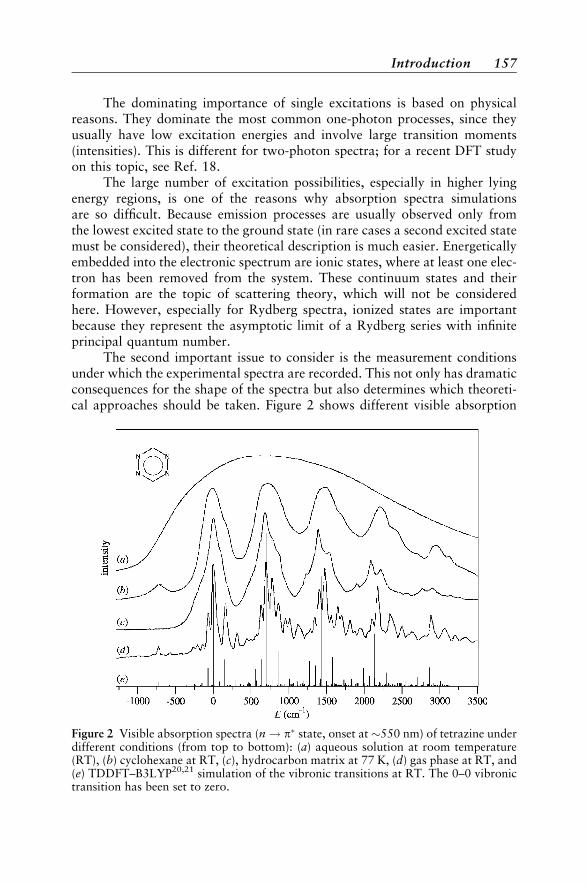
The dominating importance of single excitations is based on physicalreasons. They dominate the most common one-photon processes, since theyusually have low excitation energies and involve large transition moments(intensities). This is different for two-photon spectra; for a recent DFT studyon this topic, see Ref. 18.

The large number of excitation possibilities, especially in higher lyingenergy regions, is one of the reasons why absorption spectra simulationsare so difficult. Because emission processes are usually observed only fromthe lowest excited state to the ground state (in rare cases a second excited statemust be considered), their theoretical description is much easier. Energeticallyembedded into the electronic spectrum are ionic states, where at least one elec-tron has been removed from the system. These continuum states and theirformation are the topic of scattering theory, which will not be consideredhere. However, especially for Rydberg spectra, ionized states are importantbecause they represent the asymptotic limit of a Rydberg series with infiniteprincipal quantum number.

The second important issue to consider is the measurement conditionsunder which the experimental spectra are recorded. This not only has dramaticconsequences for the shape of the spectra but also determines which theoreti-cal approaches should be taken. Figure 2 shows different visible absorption

Figure 2 Visible absorption spectra (n! p� state, onset at �550 nm) of tetrazine underdifferent conditions (from top to bottom): (a) aqueous solution at room temperature(RT), (b) cyclohexane at RT, (c), hydrocarbon matrix at 77 K, (d) gas phase at RT, and(e) TDDFT–B3LYP20,21 simulation of the vibronic transitions at RT. The 0–0 vibronictransition has been set to zero.

Introduction 157

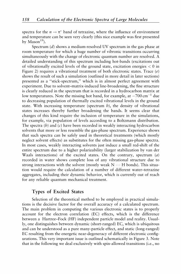
spectra for the n! p� band of tetrazine, where the influence of environmentand temperature can be seen very clearly (this nice example was first presentedby Mason19).

Spectrum (d) shows a medium-resolved UV spectrum in the gas phase atroom temperature for which a huge number of vibronic transitions occurringsimultaneously with the change of electronic quantum number are resolved. Adetailed understanding of this spectrum including hot-bands (excitations outof vibrationally excited levels of the ground state, excitation energies < 0 inFigure 2) requires a vibrational treatment of both electronic states. Trace (e)shows the result of such a simulation (outlined in more detail in later sections)presented as a ‘‘stick-spectrum,’’ which is in almost perfect agreement withexperiment. Due to solvent–matrix-induced line-broadening, the fine structureis clearly reduced in the spectrum that is recorded in a hydrocarbon matrix atlow temperatures. Note the missing hot band, for example, at �700 cm�1 dueto decreasing population of thermally excited vibrational levels in the groundstate. With increasing temperature (spectrum b), the density of vibrationalstates increases thereby further broadening the bands. It seems clear thatchanges of this kind require the inclusion of temperature in the simulations,for example, via population of levels according to a Boltzmann distribution.The spectra (b) and (c) have been recorded in weakly interacting hydrocarbonsolvents that more or less resemble the gas-phase spectrum. Experience showsthat such spectra can be safely used in theoretical treatments (which mostlyneglect solvent effects) as substitutes for the often missing gas-phase spectra.In most cases, weakly interacting solvents just induce a small red-shift of theentire spectrum due to a higher polarizability (larger stabilization by van derWaals interactions) of the excited states. On the contrary, spectrum (a)recorded in water shows complete loss of any vibrational structure due tostrong interactions with the solvent (mostly weak N � � � H bonds). This situa-tion would require the calculation of a number of different water–tetrazineaggregates, including their dynamic behavior, which is currently out of reachfor any reliable quantum mechanical treatment.

Types of Excited States

Selection of the theoretical method to be employed in practical simula-tions is the decisive factor for the overall accuracy of a calculated spectrum.The main problem in computing the various electronic states is to properlyaccount for the electron correlation (EC) effects, which is the differencebetween a Hartree–Fock (HF) independent particle model and reality. Usual-ly, one distinguishes between dynamic (short-ranged) EC, which is ubiquitousand can be understood as a pure many-particle effect, and static (long-ranged)EC resulting from the energetic near-degeneracy of different electronic config-urations. This very important issue is outlined schematically in Figure 3. Notethat in the following we deal exclusively with spin-allowed transitions (i.e., no


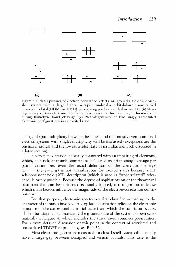
change of spin-multiplicity between the states) and that mostly even-numberedelectron systems with singlet multiplicity will be discussed (exceptions are thephenoxyl radical and the lowest triplet state of naphthalene, both discussed ina later section).

Electronic excitation is usually connected with an unpairing of electrons,which, as a rule of thumb, contributes �1 eV correlation energy change perpair. Furthermore, even the usual definition of the correlation energy(Ecorr ¼ Eexact � EHF) is not unambiguous for excited states because a HFself-consistent field (SCF) description (which is used as ‘‘uncorrelated’’ refer-ence) is rarely possible. Because the degree of sophistication of the theoreticaltreatment that can be performed is usually limited, it is important to knowwhich main factors influence the magnitude of the electron-correlation contri-butions.

For that purpose, electronic spectra are first classified according to thecharacter of the states involved. A very basic distinction relies on the electronicstructure of the corresponding initial state from which the transition occurs.This initial state is not necessarily the ground state of the system, shown sche-matically in Figure 4, which includes the three most common possibilities.For a more detailed discussion of this point in the context of restricted andunrestricted TDDFT approaches, see Ref. 22.

Most electronic spectra are measured for closed-shell systems that usuallyhave a large gap between occupied and virtual orbitals. This case is the

Figure 3 Orbital pictures of electron correlation effects: (a) ground state of a closed-shell system with a large highest occupied molecular orbital–lowest unoccupiedmolecular orbital (HOMO–LUMO) gap showing predominantly dynamic EC. (b) Near-degeneracy of two electronic configurations occurring, for example, in biradicals orduring homolytic bond cleavage. (c) Near-degeneracy of two singly substitutedelectronic configurations in an excited state.

Introduction 159

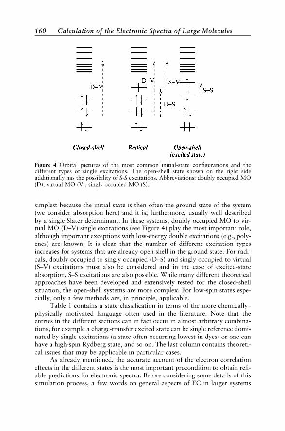
simplest because the initial state is then often the ground state of the system(we consider absorption here) and it is, furthermore, usually well describedby a single Slater determinant. In these systems, doubly occupied MO to vir-tual MO (D–V) single excitations (see Figure 4) play the most important role,although important exceptions with low-energy double excitations (e.g., poly-enes) are known. It is clear that the number of different excitation typesincreases for systems that are already open shell in the ground state. For radi-cals, doubly occupied to singly occupied (D–S) and singly occupied to virtual(S–V) excitations must also be considered and in the case of excited-stateabsorption, S–S excitations are also possible. While many different theoreticalapproaches have been developed and extensively tested for the closed-shellsituation, the open-shell systems are more complex. For low-spin states espe-cially, only a few methods are, in principle, applicable.

Table 1 contains a state classification in terms of the more chemically–physically motivated language often used in the literature. Note that theentries in the different sections can in fact occur in almost arbitrary combina-tions, for example a charge-transfer excited state can be single reference domi-nated by single excitations (a state often occurring lowest in dyes) or one canhave a high-spin Rydberg state, and so on. The last column contains theoreti-cal issues that may be applicable in particular cases.

As already mentioned, the accurate account of the electron correlationeffects in the different states is the most important precondition to obtain reli-able predictions for electronic spectra. Before considering some details of thissimulation process, a few words on general aspects of EC in larger systems

Figure 4 Orbital pictures of the most common initial-state configurations and thedifferent types of single excitations. The open-shell state shown on the right sideadditionally has the possibility of S-S excitations. Abbreviations: doubly occupied MO(D), virtual MO (V), singly occupied MO (S).


seem appropriate. Large molecules are close to a crossover region when goingfrom molecular systems to solids, and, from a physicist’s point of view wouldbe classified as insulators, semiconductors, or metals. The EC effects ininsulators (saturated with s-bonds only) are mostly local (short-ranged,dynamic) in nature and can thus be described by local wave function or densityfunctional methods. The variations of the EC effects between the differentstates of insulators are expected to be small or roughly constant so thateven simple methods completely lacking EC may be sufficient. However, thesesimple systems are not very interesting chemically and, thus, most theoreticaltreatments performed in practice must consider semiconductor- or even metal-like molecules. One characteristic of the states in these systems is the nonlocality of

Table 1 Overview of Excited-State Typesa

StateClassification Description Theoretical Aspects to Consider

Valence Excitations between Strongly varying amounts of EC(non)bonding–anti-bondingorbitals

Rydberg Excitations to virtual orbitals Special AO basis sets requiredof large spatial extent asymptotics of potentialb

Core excited Excitations out of core orbitals Special treatments–algorithmsto extract high-lying roots

Locally excited Excitations betweenspatially close orbitals

Charge transfer Excitations between Asymptotics of potentialb

very distant orbitals

Singly excited WF are dominated by Simple TD approaches sufficientc

singly excited determinantsMultiply excited WF includes important Multireference approaches

contributions from doubles, necessarytriples, and so on

Single reference WF can be described mainly by Mostly dynamic ECone determinant

Multi- WF includes many important Breakdown of MO pictureconfigurational contributions Static EC(multireference)

Low spin Spins are mostly paired EC larger for low-spin(e.g., singlet, doublet) than for high-spin states

High spin Ms > Ms (min)(e.g., triplet, quartet)

aAbbreviations: WF (wave function), EC (electron correlation), TD (time-dependent), AO(atomic orbital).

bMainly apply to TDDFT, where approximate exchange-correlation potentials are used in theeffective Kohn–Sham Hamiltonian.

cFor example, adiabatic TDDFT or LR(EOM) coupled-cluster singles and doubles.

Introduction 161

the EC (or even exchange) effects, where also a separation into static anddynamical EC is no longer appropriate. This nonlocality is difficult to describetheoretically mainly because (a) three or more particle correlations becomeimportant and (b) theoretical approximations that rely on ‘‘spatial separation’’cannot be used. Thus, only correlated wave function approaches that includethese effects explicitly will ultimately yield the desired accuracy in these cases.In this context, a strong warning should be noted: For obvious reasons, mostdevelopments of new quantum chemical methods for excited states will betested and ‘‘benchmarked’’ on atoms or small molecules with only a few elec-trons. The results and conclusions thus obtained are not always transferable to‘‘real’’ problems (i.e., a method that gives good results for ethene is not neces-sarily appropriate for porphyrin) mostly because the importance of higherorder EC effects increases with the size of the system.

THEORY

Excitation Energies

In the Born-Oppenheimer picture, electronic transitions occur between rovi-brational levels of two electronic states n and m. The excitation energy isthe energy difference between the two levels yielding the spectral position ofthe transition

�Enm;vv0; jj0 ¼ Em;v0;j0 � En;v;j ½1

where v and j indicate vibrational and rotational quantum numbers, respec-tively. Because the rotational structure is rarely resolved experimentally forlarger molecules, we always assume in the following that j ¼ j0 ¼ 0 anddrop the corresponding index. For the special case that the transition occursbetween the two vibrational ground states (v ¼ v0 ¼ 0), Eq. [1] reduces to

�E0--0nm ¼ Eel

m � Eeln þ EZPE

m � EZPEn ½2

yielding the 0–0 transition energy E0--0, where EZPE are the vibrationalzero-point energies. At low temperatures, the 0–0 transition can usually beidentified as the onset of the experimental spectrum. The calculation of thisimportant quantity thus requires the computation of the two electronic-stateenergies and their vibrational normal modes. Because the calculation ofEZPE is relatively demanding (even in the usually employed harmonic approx-imation), one often replaces the 0–0 transition energy by the pure electronicpart,

�Eelnm ¼ Eel

m � Eeln ½3


This approximation is relatively accurate yielding errors typically < 0.1–0.2 eV. If transitions from the ground state are considered, these errors aresystematic because the vibrational frequencies in the excited state are usuallysmaller than in the ground state and thus, �Eel > �E0--0.

So far, all energies discussed for the two states necessarily refer to energyminima, and thus, two separate geometry optimizations of the molecularstructures are required. While this is a routine task for most ground states,excited-state geometry optimization is a very difficult problem. First, formost of the more accurate excited-state quantum chemical models, implemen-tations of analytical gradients are still missing. Although numerical derivativescan in principle always be obtained, their calculation is usually too costly andthus they are used only for benchmark purposes on small systems.23 Second, inhigher energy regions, the density of states is usually very large, which leads tomany avoided surface crossings. In such situations, geometry optimizations arealmost impossible because state flippings often occur and induce a completebreakdown of the most common quasi-Newton optimization algorithms.These are the reasons that even today most investigations rely on the so-calledvertical approximation. In this approach, the optimized ground-state geometryis used to calculate all excited-state energies and transition moments. Notethat the vertical excitation energy

�E0elnm ¼ E

0elm � Eel

n ½4

(where the prime indicates the use of the nonrelaxed ground-state geometry)does not correspond to any observable. Instead, it represents a relatively goodapproximation (often to within 0.1–0.2 eV) to the intensity maximum of aspectral band. It should be clear that this approach works best for large mole-cules with small geometry changes between the states and for spectra obtainedin solution under low-resolution conditions. Typical values for the differencebetween vertical and 0–0 excitation energies are given in Table 3.

The ultimate goal of theoretical electronic spectroscopy is to provide reli-able and realistic simulations of electronic spectra. For that purpose, oneusually needs a relatively high accuracy for the excitation energies. If we con-sider valence and Rydberg states with �E values of < 10 eV, and if we assumetypical bandwidths of �0.3–0.5 eV, the errors for �E should not exceed 0.2–0.3 eV. Even more important than the accuracy of the absolute values (sys-tematic errors can be corrected by global shifting or scaling as is usuallydone in IR spectroscopy) is the relative accuracy obtained for the differentstates of one molecule. A wrong ordering of states can lead especially tomisinterpretation of experimental data, an issue that is a particular problemin photochemical studies.

To illustrate the accuracy that can be obtained by modern quantum che-mical methods, the results for a benchmark set of molecules is now briefly dis-cussed. An outline of the theoretical background of the applied methods is

Theory 163

given in a later section. Table 2 shows results for vertical singlet–singlet exci-tation energies obtained with TDDFT (time-dependent density functionaltheory), CC2 (a simplified coupled-cluster model), and MR-MP2 methods(multireference perturbation theory). The systems tabulated have been chosento cover a broad range of molecules and states of different character. Furtherdiscussions on the accuracy of calculated �E values are given below in thesections containing the case studies; another TDDFT benchmark study canbe found in Ref. 24.

Inspection of the data clearly shows how difficult it is to meet the accu-racy requirements of �0.2–0.3 eV even for these lowest-lying states. Althoughthe mean absolute deviation (MAD) for all three methods falls in this range,only the MR-MP2 method achieves a good overall accuracy for the entirerange of systems. Both TDDFT and CC2 have some outliers with errors

Table 2 Comparison of Calculated Vertical Singlet–Singlet Excitation Energieswith Experimental Absorption Band Maximaa

TDDFT-B3LYP CC2 MR-MP2Experimental

Molecule State (eV) Errorb (eV)

Anthracene 11B3uðpp�;LaÞ 3.3 0.03 0.69 0.3911B2uðpp�;LbÞ 3.5 0.42 0.43 �0.15

Indole 21A0ðpp�;LbÞ 4.4 0.52 0.53 �0.1531A0ðpp�;LaÞ 4.8 �0.02 0.47 0.15

Porphyrin 11B1uðpp�Þ 2.0 0.08 0.32 �0.3311B2uðpp�Þ 2.4 0.05 0.31 �0.0721B1uðpp�Þ 3.1 0.24 �0.0321B2uðpp�Þ 3.3 0.22 �0.02

Indigo 11Buðpp�Þ 2.0 0.08 0.36 0.10Pyridazine 11B2ðn! p�Þ 3.4 0.14 0.47 0.22Benzocyclo- 11B2ðn! p�Þ 2.8 0.10 0.19 �0.12

butendione11A2ðn! p�Þ 3.5 0.05 0.33 0.12

Benzaldehyde 11A00ðn! p�Þ 3.8 �0.17 0.12 0.18C5 �uðn! p�Þ 2.8 0.56 �0.19Pyrrole 11A2ðp! 3sÞ 5.2 �0.45 �0.06 0.06

11B2ðp! 3pÞ 5.9 �0.36 �0.10 0.10Si2ðCH3Þ6 1Euðs! 4pÞ 6.4 �0.38 �0.68 0.12Ferrocene 11E1gðd! dÞ 2.8 �0.79 �0.09CrðCOÞ6 11T1uðd! p�Þ 4.4 0.08 0.34

21T1uðd! p�Þ 5.5 0.50 0.10P4 11T2 5.6 �0.08 �0.08 �0.22Na4 11B3u 1.8 0.06 0.03 0.05

mean absolute deviation (MAD) 0.24 0.32 0.15

aFor technical details and references to the experimental data see Ref. 25.bError ¼ �Eðcalc:Þ ��Eðexp :Þ.


>0:5 eV and CC2, especially, completely breaks down for C5 and the difficulttransition metal systems. Note that the three methods tested represent themost accurate approaches that can also be applied to larger systems andthat other ‘‘cheap’’ methods (like CIS or semiempirical treatments) often yieldquite unreliable results with errors >0.5–1 eV.

As already mentioned, a direct comparison of vertical excitation energieswith experimental data is not possible and such results contain uncertaintiesdue to geometry relaxation effects. A more reliable assessment of theoreticalmethods can be achieved by a comparison of the �E0--0 values that arepresented for the lowest states of some unsaturated molecules in Table 3.The last column of this table indicates the difference between 0–0 and verticalexcitation energies.

These data indicate more clearly the problems theoretical methods(TDDFT in this case) have in accounting for the change of electronic structureupon excitation. For the ionic La states of the aromatic compounds (usingPlatts nomenclature derived from the perimeter model, see, Ref. 9 e.g.) andthe 1Bu state of the polyene, a systematic underestimation of the excitationenergies is observed while the opposite is true for the other more covalentstates that exhibit stronger multiconfigurational character (for a more detaileddiscussion of these problems see Refs. 35 and 36).

The effects of geometry relaxation (sixth column) are significant for thesmaller and medium-sized systems (0.4–0.6 eV) but diminish with the size ofthe molecule. For the larger aromatic molecules, differences between �E

0el and�E0--0 of �0.2–0.3 eV are found. Note, however, that the geometry relaxationeffects can be more important (up to 1 eV) in the case of larger systems as wellwhen single-bond torsions between conjugated fragments are possible.37 Thedifferences between the �Eel and �E0--0 values (the ZPE contribution) aremuch smaller (0.12–0.17 eV, 0.03 eV for azulene) and roughly constant forthe systems considered.

Transition Moments

Band intensities (transition probabilities) are the second important factordetermining the shape of an electronic spectrum. Including the oscillatingradiation field as a perturbation to the molecular Hamiltonian and applyingtime-dependent perturbation theory yields, under some approximations (themost important being that the radiation wavelength is much larger than thesize of the molecule and small field strengths), the electronic transitionmoment (TM) as an expectation value over the initial and final wave functionswith the relevant one-electron operator OO,

TM ¼ �mjOOj�n

D E½5

Theory 165

Table

3C

om

pari

son

of

Calc

ula

ted

[TD

DFT

-B3L

YP/T

ZV

(d,p

)]and

Exper

imen

tal

0–0

Exci

tati

on

Ener

gie

s(i

neV

)fo

rth

eL

ow

est

Sin

gle

tSta

tes

(pp�

)of

Unsa

tura

ted

Syst

ems �

E0--

0�

E0e

l��

E0--

0

Mole

cule

Tra

nsi

tion

Calc

.E

xp.

Err

or

Calc

.C

ondit

ions

Ref

eren

ce

Naphth

ale

ne

1B

2u;L

a3.9

84.4

4�

0.4

60.4

2G

as

phase

26

Anth

race

ne

1B

2u;L

a2.9

03.4

3�

0.5

30.3

3G

as

phase

26

Tet

race

ne

1B

2u;L

a2.1

82.7

7�

0.5

90.2

9A

rgon

jet

27

Pen

tace

ne

1B

2u;L

a1.6

62.1

2�

0.4

60.3

3H

exadec

ane

matr

ix28

Pyre

ne

1B

2u;L

a3.4

33.8

4�

0.4

10.2

6G

as

phase

26

Azu

lene

1B

11.9

91.7

80.2

10.4

1C

ycl

ohex

ane

29

Oct

ate

traen

e1B

u3.7

14.4

1�

0.7

00.3

4A

rgon

jet

30

Oct

ate

traen

e2A

g4.4

63.5

90.8

70.4

5H

eliu

mje

t31

Sty

rene

2A0

4.4

14.8

8�

0.4

60.5

6A

rgon

jet

32

Phen

ol

2A0 ;

Lb

4.7

94.5

10.2

80.3

1A

rgon

jet

33

o-C

yanophen

ol

2A0 ;

Lb

4.3

24.2

10.1

10.3

1H

eliu

mje

t34

166

A comprehensive discussion of this important derivation can be found inRefs. 38 and 39. The nuclear contributions to the TM leading to vibrationalfine structure in the spectra are discussed in the following section. Alterna-tively, the electronic part of the TM is obtained from the first-order reducedtransition density matrix c as

TM ¼ trðOcÞ ½6

where the matrix O is the representation of the operator in the basis of orbitalsc (Oij ¼

ÐciðrÞOOcjðrÞdr) and c is the analogous matrix representation of the

transition density given by

gij ¼ðciðr1Þgðr1; r

01Þcjðr01Þdr1dr01 ½7

with

gðr1; r01Þ ¼ Nel

ð�m�ndr2 � � � drN ½8

The importance of the concept of transition density matrices is that they allowa straightforward interpretation of excited states13 either by plotting or bypopulation analyses as usually performed for ‘‘normal’’ (n ¼ m) densities.

The leading term in the interaction of radiation with matter is the electricdipole contribution (l) for which the one-electron operator OO is given by theposition coordinates rk of the electrons as

OO � llL ¼ eXNel

k

rrk ½9

which is called the ‘‘dipole-length’’ form. Note that l are vector quantities(given in bold) including x, y, and z components. The alternative ‘‘velocity’’formulation uses

OO � llV ¼�ie

�Eel

XNel

k

==k ½10

For exact wave functions and those that fulfill the hyper-virial theorem byconstruction [e.g., time-dependent Hartree–Fock (TDHF) or random phaseapproximation (RPA), TDDFT, see below] both forms are equivalent. Notethat all virial theorems are exactly fulfilled only in a complete (i.e., usuallyinfinitely large) AO basis. By a simultaneous computation of the transitiondipole moments in the length and velocity forms and subsequent numerical

Theory 167

comparison, the above mentioned time dependent (TD) methods allow someestimate of basis set completeness for the corresponding transition. Table 4provides a numerical comparison of the two transition dipole moments forthe weakly allowed n! p� transition in acetaldehyde calculated with differentAO basis sets.

It can be seen that if a certain degree of basis set saturation is reached(cc-pVTZ, third row), the two values start to converge to the same value(�0.067), which is almost reached at the aug-cc-pVTZ level. Note the strongeffect of ‘‘diffuse’’ functions (denoted as aug) for this property (compare rowsthree/four and five/six) and also the relatively large fluctuations for the velocityform that are caused by the more complicated structure of the differentialoperator in Eq. [10]. In addition, there is a lot of numerical evidence thatfor other systems the length form is more stable yielding, with small AO basissets, results closer to the basis set limit (see, e.g., Ref. 42). Note too that thepresented example is quite challenging due to the ‘‘almost’’ symmetry forbid-den character of the transition and that both the fluctuations for the V-formare smaller and the agreement between L- and V-forms is better for dipoleallowed transitions.

The (dimensionless) oscillator strength for an electronic transition isgiven by

fnm ¼2

3�Enmjlnmj

2 ½11

where �E and the length of the transition dipole vector are expressed in atomicunits. Theoretically, f ¼ 1 corresponds to the transition probability of a har-monically moving electron bound to a proton (an early model of the hydrogenatom). Experimentally, one obtains f by integrating the area under the absorp-tion band between energies �nn1 and �nn2 (in wavenumbers)

f ¼ 4:3� 10�9

ð�nn2

�nn1

eð�nnÞd�nn ½12

Table 4 The TDHF Transition Dipole Moments (in Debye) for the 11A0 ! 11A00

Transition (n! p� excited state) in Acetaldehyde Calculated withDunning’s Correlation Consistent cc-VXZ Basis Setsa

Basis Set mV mL

cc-VDZ ½3s2p=2s 0.0701 0.0363cc-pVDZ ½3s2p1d=2s1p 0.0072 0.0330cc-pVTZ ½4s3p2d1f=3s2p1d 0.0317 0.0534aug-cc-pVTZ ½4s3p2d1f=3s2p1d þ ½1s1p1d1f=1s1p1d 0.0695 0.0674cc-pVQZ ½5s4p3d2f1g=4s3p2d1f 0.0513 0.0591aug-cc-pVQZ ½5s4p3d2f1g=4s3p2d1f þ ½1s1p1d1f1g=1s1p1d1f 0.0675 0.0670

aSee Refs. 40 and 41.


where e is the decadic molar extinction coefficient given in L/(mol cm).Although in experimental investigations a nonlinear energy scale l ¼ hc=E(wavelengths) is usually used, it is strongly recommended that one transformall data (experimental and theoretical) first to linear eV or cm�1 units. Inver-sion of Eq. [12] allows one to deduce eð�nnÞ from calculated oscillator strengths.For the band form of the individual transitions (also called ‘‘shape-function’’),Gaussian functions have been successfully employed, which accounts forvibrational (and solvent, if present) induced broadening. To simulate entirespectra, the contributions from all transitions are added according to

eðEÞ ¼ 2:87� 104ffiffiffiffisp

Xi

fie�ðE��EiÞ=2s½ 2 ½13

where s is the full width of the band at 1=e height (for most UV bands s ¼ 0:4eV is appropriate) and �Ei (in eV) and fi are the excitation energies and oscil-lator strengths for transition i, respectively. Figure 5 schematically shows atypical outcome for the simulation of a conventional UV spectrum. The verti-cal lines indicate the position and oscillator strength of the individual transi-tions (right f axis), while the dashed curve is the overall result from Eq. [13].Very weak or forbidden transition should be indicated by special symbols.

E [eV]

0

20000

40000

60000

80000

ε [l/

mol

cm

] 1.0

0.8

0.6

0.4

0.2

osci

llato

r st

reng

th

forb

idde

n tr

ansi

tion

Figure 5 Example of the graphical presentation of a simulated (vertical) UV spectrum.

Theory 169

For an electric dipole allowed transition, the radiation field must createor destroy a node in the corresponding transition density. A simple example isan atomic s! p excitation, where the transition density is simply given by theproduct s� p, which yields a scalar quantity when multiplied by r and inte-grated over space. In other words, the transition density must have a dipolarstructure, where ‘‘probability’’ is shifted from positive-to-negative (andvice versa) regions. The mathematical process of generating the electric dipoletransition moments is schematically outlined for the example of the p! p�

transition of ethene in Figure 6.If the transition density simultaneously has some rotational character,

the magnetic component of the radiation field becomes important. For noncir-cularly polarized light, that is, in conventional UV spectroscopy, the magneticcomponent of the radiation field can be neglected in the time-dependent per-turbation because it enters with a factor vav

el =c; the average electron velocity ismuch smaller than the speed of light. The effect of the magnetic component incircularly polarized light is observed experimentally in electronic circulardichroism (CD) spectroscopy of chiral molecules.43 As a conventional absorp-tion, it is a first-order, linear effect but depends on the combined interaction ofa molecule with the electric and magnetic components of the radiation field.

The main quantity in CD is the rotatory strength R, which is completelyanalogous to the oscillator strength in UV spectroscopy and is given by thescalar product44,45

Rnm ¼ Imh�njllj�mi � h�njmmj�mi¼ jlnmj � jmnmj � cosðlnm;mnmÞ ½14

Figure 6 Schematic description for the process of generating the electric transitiondipole moment for the p! p� excitation of ethene. Transparent (black) areascorrespond to a positive (negative) phase.


where mm is the magnetic dipole operator (angular momentum)

mm ¼ �he

2mci

XNel

k

rrk � ==k ½15

In oriented media (which will not be considered here), additional dipole–quad-rupole terms contribute to the CD. The rotatory strength is zero by symmetryif the molecule possesses at least one improper Sn axis as symmetry element(this causes either m or m to be zero or an orthogonal arrangement of thetwo vectors, see Eq. [14]). Also, in complete analogy to UV spectra, R canbe obtained from Eq. [12] with e replaced by the difference of extinction coef-ficients for left- and right-circularly polarized light (�e ¼ eL � eR).

The main perspective of CD spectroscopy is its potential to determine theabsolute configurations of chiral substances that is of particular importancefor compounds with biological or pharmacological relevance, for example.Furthermore, unlike optical spectra, the CD bands can be positive or negative,and for this reason carry more information and sometimes allow one toresolve close-lying or hidden electronic transitions. More details abouttheoretical CD spectroscopy can be found in Refs. 43 and 46–48. In Ref. 49the CD spectra of a benchmark set of molecules have been investigated with themost recent quantum chemical methods. Some representative examples arediscussed in a later section of this chapter. Recent advances in the theoreticaldescription of magnetically induced CD, which in addition employs a staticmagnetic field, can be found in Ref. 50.

Vibrational Structure

In general, the intensity I of a transition between the two states �m and�n is proportional to the square of the transition dipole moment

ln;m ¼ h�njllj�mi ½16

with the dipole operator

ll ¼ �eX

i

rri þ eX

s

ZsRRs ¼ lle þ llN ½17

where rri and RRs denote the electron and nuclear coordinates, respectively, andZs represents the nuclear charges.

For the description of a vibronic transition both electronic and nuclearcoordinates must be taken into account. In the adiabatic BO approximation,the complete wave function can be separated into the product

�ðr;RÞ ¼ �eðr;RÞ�NðRÞ ½18

Theory 171

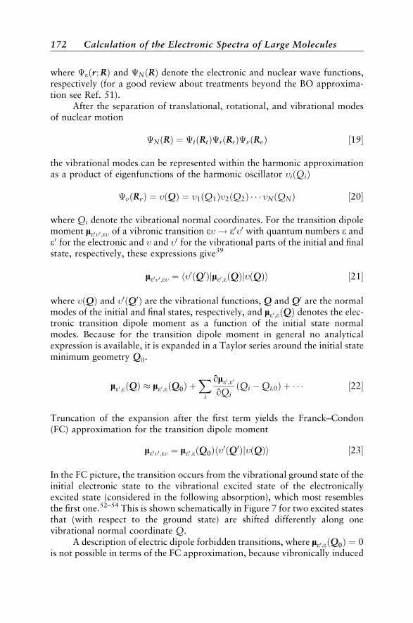
where �eðr;RÞ and �NðRÞ denote the electronic and nuclear wave functions,respectively (for a good review about treatments beyond the BO approxima-tion see Ref. 51).

After the separation of translational, rotational, and vibrational modesof nuclear motion

�NðRÞ ¼ �tðRtÞ�rðRrÞ�vðRvÞ ½19

the vibrational modes can be represented within the harmonic approximationas a product of eigenfunctions of the harmonic oscillator �iðQiÞ

�vðRvÞ ¼ �ðQÞ ¼ �1ðQ1Þ�2ðQ2Þ � � � �NðQNÞ ½20

where Qi denote the vibrational normal coordinates. For the transition dipolemoment le0�0;e� of a vibronic transition e�! e0�0 with quantum numbers e ande0 for the electronic and � and �0 for the vibrational parts of the initial and finalstate, respectively, these expressions give39

le0�0;e� ¼ h�0ðQ0Þjle0;eðQÞj�ðQÞi ½21

where �ðQÞ and �0ðQ0Þ are the vibrational functions, Q and Q0 are the normalmodes of the initial and final states, respectively, and le0;eðQÞ denotes the elec-tronic transition dipole moment as a function of the initial state normalmodes. Because for the transition dipole moment in general no analyticalexpression is available, it is expanded in a Taylor series around the initial stateminimum geometry Q0.

le0;eðQÞ � le0;eðQ0Þ þX

i

qle0;e0

qQiðQi �Qi;0Þ þ � � � ½22

Truncation of the expansion after the first term yields the Franck–Condon(FC) approximation for the transition dipole moment

le0�0;e� ¼ le0;eðQ0Þh�0ðQ0Þj�ðQÞi ½23

In the FC picture, the transition occurs from the vibrational ground state of theinitial electronic state to the vibrational excited state of the electronicallyexcited state (considered in the following absorption), which most resemblesthe first one.52–54 This is shown schematically in Figure 7 for two excited statesthat (with respect to the ground state) are shifted differently along onevibrational normal coordinate Q.

A description of electric dipole forbidden transitions, where le0;eðQ0Þ ¼ 0is not possible in terms of the FC approximation, because vibronically induced


transition moments are neglected. Truncation of the Taylor expansion(Eq. [22]) after the second term yields the Franck–Condon–Herzberg–Teller(FC–HT) approximation for the transition dipole moment

le0�0;e� ¼ le0;eðQ0Þh�0ðQ0Þj�ðQÞi þX

i

qle0;e

qQih�0ðQ0ÞjðQi �Qi;0Þj�ðQÞi ½24

This description accounts for transition dipole moments induced by displace-ments along the normal modes during the electronic transition, that is, a simul-taneous excitation of vibrational modes. This approximation is also denotedas double-harmonic. For electric dipole forbidden transitions, the first term inEq. [24] vanishes and the resulting expression is denoted as the Herzberg-Teller (HT) approximation.

le0�0;e� ¼X

i

qle0;e0

qQih�0ðQ0ÞjðQi �Qi;0Þj�ðQÞi ½25

Figure 7 Schematic description of the FC principle for two excited states withdominating 0–0 transition (�2, almost parallel potential surfaces) and a broad intensitydistribution (�1, shifted minimum), respectively. The nonzero intensities for 0–1,0–2, . . . vibrational transitions to �2 result entirely from the different shapes of thesurfaces, while the intensity distribution for the other transition originates mainly fromthe shifted minimum.

Theory 173

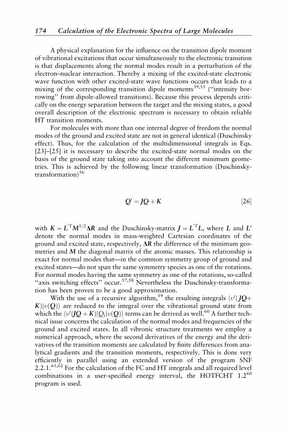
A physical explanation for the influence on the transition dipole momentof vibrational excitations that occur simultaneously to the electronic transitionis that displacements along the normal modes result in a perturbation of theelectron–nuclear interaction. Thereby a mixing of the excited-state electronicwave function with other excited-state wave functions occurs that leads to amixing of the corresponding transition dipole moments39,55 (‘‘intensity bor-rowing’’ from dipole-allowed transitions). Because this process depends criti-cally on the energy separation between the target and the mixing states, a goodoverall description of the electronic spectrum is necessary to obtain reliableHT transition moments.

For molecules with more than one internal degree of freedom the normalmodes of the ground and excited state are not in general identical (Duschinskyeffect). Thus, for the calculation of the multidimensional integrals in Eqs.[23]–[25] it is necessary to describe the excited-state normal modes on thebasis of the ground state taking into account the different minimum geome-tries. This is achieved by the following linear transformation (Duschinsky-transformation)56

Q0 ¼ JQþ K ½26

with K ¼ L0TM1=2DR and the Duschinsky-matrix J ¼ L

0TL, where L and L0

denote the normal modes in mass-weighted Cartesian coordinates of theground and excited state, respectively, DR the difference of the minimum geo-metries and M the diagonal matrix of the atomic masses. This relationship isexact for normal modes that—in the common symmetry group of ground andexcited states—do not span the same symmetry species as one of the rotations.For normal modes having the same symmetry as one of the rotations, so-called‘‘axis switching effects’’ occur.57,58 Nevertheless the Duschinsky-transforma-tion has been proven to be a good approximation.

With the use of a recursive algorithm,59 the resulting integrals h�0ð JQþKÞj�ðQÞi are reduced to the integral over the vibrational ground state fromwhich the h�0ðJQþ KÞjQij�ðQÞi terms can be derived as well.60 A further tech-nical issue concerns the calculation of the normal modes and frequencies of theground and excited states. In all vibronic structure treatments we employ anumerical approach, where the second derivatives of the energy and the deri-vatives of the transition moments are calculated by finite differences from ana-lytical gradients and the transition moments, respectively. This is done veryefficiently in parallel using an extended version of the program SNF2.2.1.61,62 For the calculation of the FC and HT integrals and all required levelcombinations in a user-specified energy interval, the HOTFCHT 1.260

program is used.


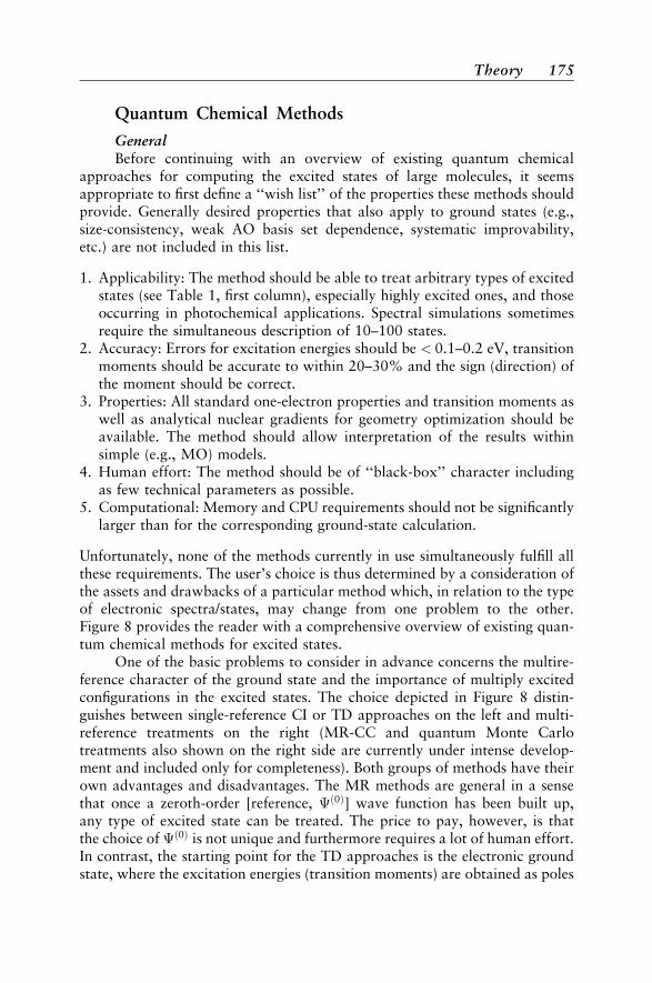
Quantum Chemical Methods

GeneralBefore continuing with an overview of existing quantum chemical

approaches for computing the excited states of large molecules, it seemsappropriate to first define a ‘‘wish list’’ of the properties these methods shouldprovide. Generally desired properties that also apply to ground states (e.g.,size-consistency, weak AO basis set dependence, systematic improvability,etc.) are not included in this list.

1. Applicability: The method should be able to treat arbitrary types of excitedstates (see Table 1, first column), especially highly excited ones, and thoseoccurring in photochemical applications. Spectral simulations sometimesrequire the simultaneous description of 10–100 states.

2. Accuracy: Errors for excitation energies should be < 0.1–0.2 eV, transitionmoments should be accurate to within 20–30% and the sign (direction) ofthe moment should be correct.

3. Properties: All standard one-electron properties and transition moments aswell as analytical nuclear gradients for geometry optimization should beavailable. The method should allow interpretation of the results withinsimple (e.g., MO) models.

4. Human effort: The method should be of ‘‘black-box’’ character includingas few technical parameters as possible.

5. Computational: Memory and CPU requirements should not be significantlylarger than for the corresponding ground-state calculation.

Unfortunately, none of the methods currently in use simultaneously fulfill allthese requirements. The user’s choice is thus determined by a consideration ofthe assets and drawbacks of a particular method which, in relation to the typeof electronic spectra/states, may change from one problem to the other.Figure 8 provides the reader with a comprehensive overview of existing quan-tum chemical methods for excited states.

One of the basic problems to consider in advance concerns the multire-ference character of the ground state and the importance of multiply excitedconfigurations in the excited states. The choice depicted in Figure 8 distin-guishes between single-reference CI or TD approaches on the left and multi-reference treatments on the right (MR-CC and quantum Monte Carlotreatments also shown on the right side are currently under intense develop-ment and included only for completeness). Both groups of methods have theirown advantages and disadvantages. The MR methods are general in a sensethat once a zeroth-order [reference, �ð0Þ] wave function has been built up,any type of excited state can be treated. The price to pay, however, is thatthe choice of �ð0Þ is not unique and furthermore requires a lot of human effort.In contrast, the starting point for the TD approaches is the electronic groundstate, where the excitation energies (transition moments) are obtained as poles

Theory 175

Fig

ure

8A

nover

vie

wofquantu

mch

emic

alm

ethods

for

exci

ted

state

s.B

old

-ita

lic

entr

ies

indic

ate

met

hods

thatare

curr

entl

yappli

cable

tola

rge

mole

cule

s.Im

port

ant

abbre

via

tions

use

d:C

I(c

onfigura

tion

Inte

ract

ion),

TD

(tim

e-dep

enden

t),C

C(c

ouple

d-c

lust

er),

HF

(Hart

ree–

Fock

),C

AS

(com

ple

teact

ive

space

),R

AS

(res

tric

ted

act

ive

space

),M

P(M

øll

er–Ple

sset

per

turb

ati

on

theo

ry),

S(s

ingle

sex

cita

tion),

SD

(sin

gle

sand

double

sex

cita

tion),

MR

(mult

iref

eren

ce).

Geo

met

ryopti

miz

ati

ons

ofex

cite

dst

ate

sfo

rla

rger

mole

cule

sare

now

poss

ible

wit

hC

IS,

CA

SSC

F,

CC

2,

and

TD

DFT

met

hods.

176

(residuals) of the response of the ground state to a time-dependent perturba-tion (electric field).

The basic theoretical background of the most widely used methodswill be outlined in the following sections including the most important work-ing equations and technical issues that must be considered in large-scale appli-cations.

CI MethodsAlthough the application of configuration interaction (CI) methods to

excited-state problems has decreased in recent years, they should be consid-ered here first because the formalism is easy to understand and if properlydeveloped, are also most general in application. A recent comprehensivereview can be found in Ref. 63.

All CI methods are variational, that is, the electronic Schr€odingerequation

HHj�CIn i ¼ ECI

n j�CIn i ½27

is solved for state n with the following ansatz for the wave function

j�CIn i ¼ ðTT1 þ TT2 þ TT3 þ � � �Þj�ð0Þi ½28

where �ð0Þ is a so-called reference wave function and TTk are the single (one-electron, k ¼ 1), double (two-electron, k ¼ 2) and triple (three-electron, k¼3)excitation (replacement) operators, respectively. By acting onto �ð0Þ theseoperators generate complete sets of (excited) determinants by substitutionsof occupied orbitals i; j; k; . . . in the determinants of �ð0Þ with virtual orbitalsb; c; d; . . .. Note that in general, open-shell determinants are not eigenfunc-tions of the SS2 operator (they cannot be classified according to multiplicityas, e.g., singlet, doublet, triplet, . . .). Actual treatments are often based onso-called configuration-state functions (CSF), which are represented by appro-priate linear combinations of several determinants with the same Ms value (theterm ‘‘configuration’’, which is often used to characterize the spatial distribu-tion of the electrons in the different orbitals, is merely used linguistically butcannot be employed in actual computations).

The most important contributions from singles and doubles excitationare given, for example, by

TT1 ¼X

ib

tbi aia

yb ½29

TT2 ¼1

4

Xibjc

tbcij aia

ybaja

yc ½30

Theory 177

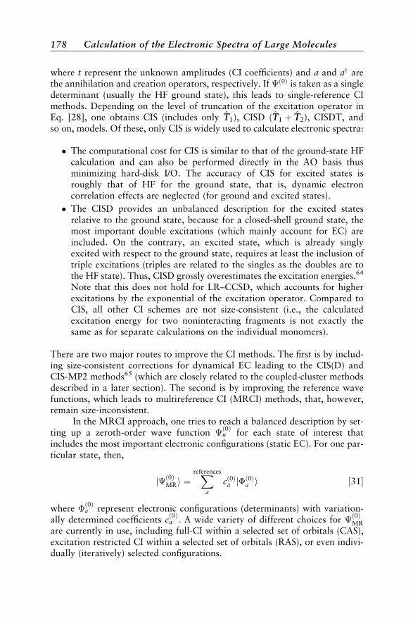
where t represent the unknown amplitudes (CI coefficients) and a and ay arethe annihilation and creation operators, respectively. If �ð0Þ is taken as a singledeterminant (usually the HF ground state), this leads to single-reference CImethods. Depending on the level of truncation of the excitation operator inEq. [28], one obtains CIS (includes only TT1), CISD (TT1 þ TT2), CISDT, andso on, models. Of these, only CIS is widely used to calculate electronic spectra:

� The computational cost for CIS is similar to that of the ground-state HFcalculation and can also be performed directly in the AO basis thusminimizing hard-disk I/O. The accuracy of CIS for excited states isroughly that of HF for the ground state, that is, dynamic electroncorrelation effects are neglected (for ground and excited states).

� The CISD provides an unbalanced description for the excited statesrelative to the ground state, because for a closed-shell ground state, themost important double excitations (which mainly account for EC) areincluded. On the contrary, an excited state, which is already singlyexcited with respect to the ground state, requires at least the inclusion oftriple excitations (triples are related to the singles as the doubles are tothe HF state). Thus, CISD grossly overestimates the excitation energies.64

Note that this does not hold for LR–CCSD, which accounts for higherexcitations by the exponential of the excitation operator. Compared toCIS, all other CI schemes are not size-consistent (i.e., the calculatedexcitation energy for two noninteracting fragments is not exactly thesame as for separate calculations on the individual monomers).

There are two major routes to improve the CI methods. The first is by includ-ing size-consistent corrections for dynamical EC leading to the CIS(D) andCIS-MP2 methods65 (which are closely related to the coupled-cluster methodsdescribed in a later section). The second is by improving the reference wavefunctions, which leads to multireference CI (MRCI) methods, that, however,remain size-inconsistent.

In the MRCI approach, one tries to reach a balanced description by set-ting up a zeroth-order wave function �

ð0Þn for each state of interest that

includes the most important electronic configurations (static EC). For one par-ticular state, then,

j�ð0ÞMRi ¼Xreferences

a

cð0Þa jð0Þa i ½31

where ð0Þa represent electronic configurations (determinants) with variation-

ally determined coefficients cð0Þa . A wide variety of different choices for �

ð0ÞMR

are currently in use, including full-CI within a selected set of orbitals (CAS),excitation restricted CI within a selected set of orbitals (RAS), or even indivi-dually (iteratively) selected configurations.


Application of this ansatz together with the truncation to single and dou-ble excitations as before (Eq. [28]) now includes all important contributions ina balanced manner. Hence, for a singly excited state, important parts of thetriple excitations are included. The MR(SD)CI (the SD term is usuallydiscarded in the abbreviation) method is very accurate for small- and med-ium-sized systems when the remaining size-consistency errors are correctedempirically, for example, via the Davidson scheme. Unfortunately, it is com-putationally very demanding to have an N6

el scaling behavior with system sizeand a very large prefactor. It can be routinely applied only to systems with�20–40 electrons (for benchmark or calibration purposes). For a more effi-cient approach that empirically combines DFT and MRCI methods, andthat can be applied also to large systems see Ref. 66, applications in electronicspectroscopy can be found in Refs. 67–71.

Perturbation MethodsOne way to retain the generality of the MR ansatz while reducing the

computational costs is to use perturbation theory (PT). Perturbation theoryhas the important property of being size-consistent if properly formulatedand implemented.72 The starting point is again a reference wave function�ð0Þn for a particular electronic state n that includes the most important contri-

butions to the wave function. By construction, �ð0Þn satisfies the eigenequation

HH0j�ð0Þn i ¼ Eð0Þn j�ð0Þn i ½32�

where HH0 is the zeroth-order Hamiltonian. In MP partitioning, HH0 is definedvia the perturbation V, which is

lVV ¼ HH HH0 ¼XNel

i

XNel

j>i

1=rrij VVee

D Eaverage

½33�

the difference between the true and the mean-field (HF) electron–electronrepulsion. In the MP schemes, HH0 is represented as a sum of general Fockoperators that are state-dependent. As usual in perturbation theory, the energyand wave function are expanded in a Taylor series for l that then leads to a(decoupled) system of linear equations for each perturbation order. For largesystems, one usually truncates at second-order (for an approximate fourth-order treatment see Ref. 73) which leads to methods that scale as N5

el withthe system size. The second-order energy correction Eð2Þ is

Eð2Þ ¼ X

a

tð1Þa h�ð1Þa jHHj�ð0Þn i ½34�

Theory 179

where ð1Þa is an element (CSF) of the first-order corrected wave function with

amplitude tð1Þa that is obtained by solving the linear equations

Xa

tð1Þa hð1Þb jHH0 � Eð0Þn jð1Þa i ¼ �h

ð1Þb jHHj�

ð0Þn i ½35

In general, �ð1Þ ¼P

a tð1Þa

ð1Þa contains all single and double excitations from

the reference that directly interacts through the true operator HH [the variousvariants of MRPT differ in how the annihilation and creation operators act on�ð0Þ].

A key point here is that in contrast to the MRCI case, the very largeinteraction matrix contains only elements between CSF and the simple one-electron operator HH0 (the costly interactions with HH appear only on the rightside of Eq. [35] with the reference). This not only decreases the scaling beha-vior from N6

el (CI) to N5el (PT), but also reduces the computational effort

considerably because the one-electron matrix elements are very easy toevaluate. Apart from technical details for the solution of Eq. [35] (whichespecially holds for CASPT2, which uses a density matrix approach74),the different implementations of multireference perturbation theory(CASPT2,74–76 CASMP2,77 MR-MP278) differ mainly by the choice ofthe reference wave function. Both CASPT2 and CASMP2 are based oncomplete-active-space wave functions as references that consist of a full CItreatment within an active space of orbitals–electrons and state-optimizedorbitals while the MR-MP2 variant can employ arbitrary CI references andorbital sets. To be applicable for large molecules, careful consideration of tech-nical details and implementation is necessary: There are at least twoapproaches76,78 that have demonstrated good accuracy at reduced computa-tional costs.

Within the ‘‘ab initio world’’, CASPT2 became the de facto standard bychemists for the calculation of electronic spectra. Its first success was the accu-rate description of the electronic spectrum of benzene,75 which at that timewas a challenging goal for quantum chemistry. Since then, hundreds of appli-cations of CASPT2 in electronic spectroscopy appeared that are described inexisting reviews10–12 (for the most recent application see Ref. [79]). The mostsevere drawback of CASPT2 is the full CI reference wave function on which itis based. Without symmetry, active spaces of 12 electrons in 12 orbitals in thepreceeding CASSCF treament are the current limit that is often not enough forlarge unsaturated systems.

TDHF and TDDFTIt is an understatement to say that DFT80,81 has strongly influenced the

evolution of quantum chemistry during the past 10–15 years. In the last 5years, this statement also holds true for the treatment of excited states and,since then, time-dependent Kohn–Sham (KS) DFT (TDDFT)[82,83] has


become a routine tool to simulate electronic spectra. Both TDDFT and TDHFmethods can be derived along similar lines as outlined briefly below.

We consider an N-electron system that is initially at time t ¼ t0 in itsground state j�0i. At times t > t0 a time-dependent perturbation lUUðtÞ isapplied. For our purposes, the most important perturbation is the electricdipole part (l) of a monochromatic radiation field given by

UUðtÞ ¼ �lEe�iot ½36

that oscillates with frequency o and has a (constant) field strength E. Thelinear response (LR) [index ð1Þ] of an observable OðtÞ is defined as the firstvariation of the expectation value with respect to the scalar variable l

Oð1ÞðtÞ ¼ dh�ðtÞjOOðtÞj�ðtÞi ¼ d

dlh�ðtÞjOOðtÞj�ðtÞijl¼0 ½37

where �ðtÞ is the time-dependent (ground-state) wave function. Graphically,we can imagine that �ðtÞ can be represented by the complete set of all excitedeigenstates (including �0) of the Hamiltonian and, thus, one can derive infor-mation about the desired excited states by considering the time evolution of�ðtÞ. More precisely, at certain frequencies o electronic transitions are stimu-lated and the first-order response of the ground state must diverge. For thesevalues of o, the first-order response equations are exactly satisfied even if lE iszero, since these are intrinsic molecular properties corresponding to free oscil-lations. In other words, solving the TD equations for some Hamiltonian with aparticular ansatz for the ground-state wave function is equivalent to findingthe poles of the frequency-dependent polarizability aðoÞ (see Figure 9) thatis given by the sum-over-states formula

aðoÞ ¼Xall excited states

n

f0n

o2n � o2

½38

The transition moment can be obtained as the residue given by

h�0jlj�ni ¼ limo!on

ðo� onÞaðoÞ ½39

Both the DFT and HF methods use an effective, one-particle (mean-field)Fock operator F. In general, it can be written as a functional of the first-orderdensity matrix g (see Eq. [8] with m ¼ n ¼ 0) as

F½gðtÞ ¼ h½gðtÞ þ vH½gðtÞ � vxc½gðtÞ þ lUðtÞ ½40

Theory 181

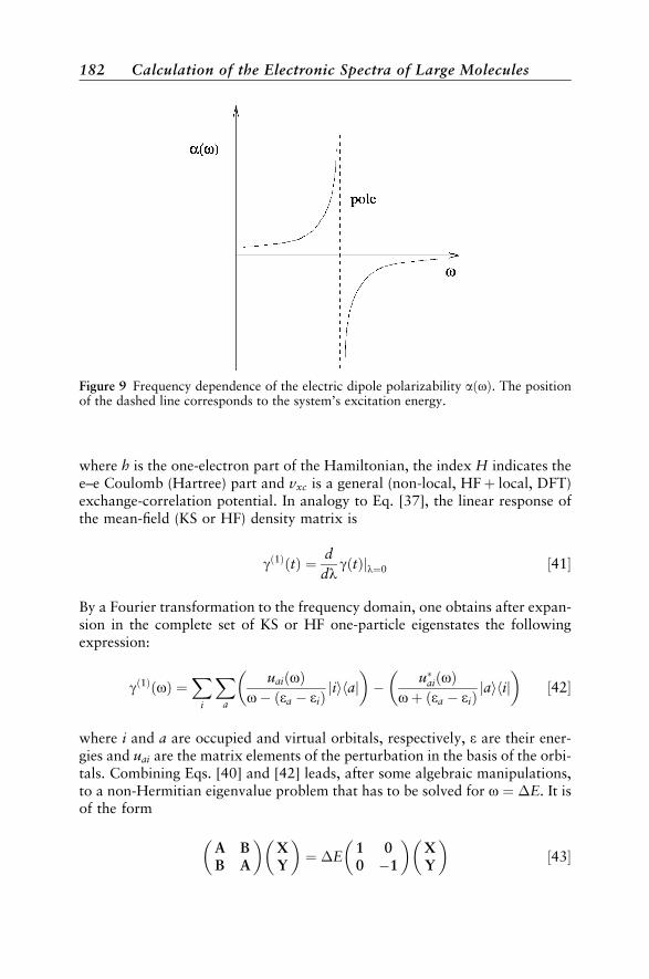
where h is the one-electron part of the Hamiltonian, the index H indicates thee–e Coulomb (Hartree) part and vxc is a general (non-local, HFþ local, DFT)exchange-correlation potential. In analogy to Eq. [37], the linear response ofthe mean-field (KS or HF) density matrix is

gð1ÞðtÞ ¼ d

dlgðtÞjl¼0 ½41

By a Fourier transformation to the frequency domain, one obtains after expan-sion in the complete set of KS or HF one-particle eigenstates the followingexpression:

gð1ÞðoÞ ¼X

i

Xa

uaiðoÞo� ðea � eiÞ

jiihaj�

� u�aiðoÞoþ ðea � eiÞ

jaihij�

½42

where i and a are occupied and virtual orbitals, respectively, e are their ener-gies and uai are the matrix elements of the perturbation in the basis of the orbi-tals. Combining Eqs. [40] and [42] leads, after some algebraic manipulations,to a non-Hermitian eigenvalue problem that has to be solved for o ¼ �E. It isof the form

A BB A

� XY

� ¼ �E

1 00 �1

� XY

� ½43

Figure 9 Frequency dependence of the electric dipole polarizability aðoÞ. The positionof the dashed line corresponds to the system’s excitation energy.


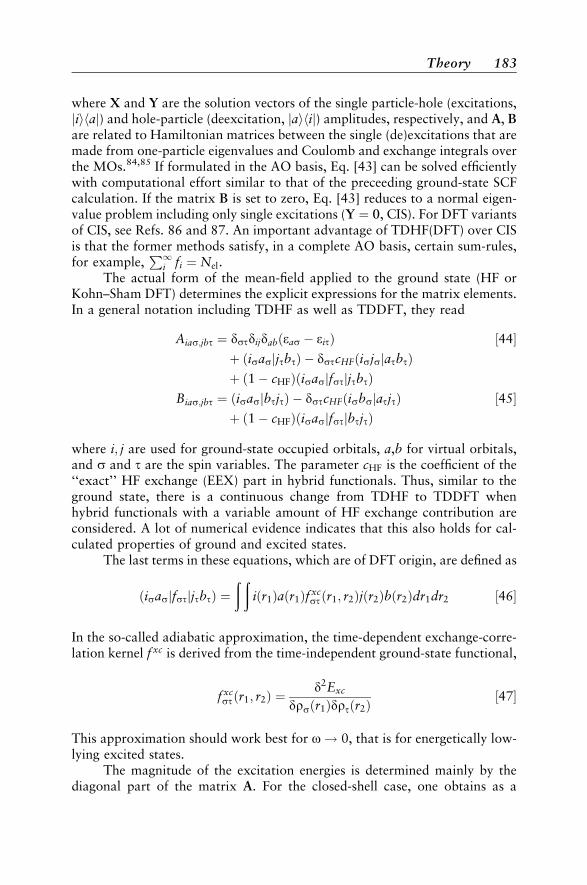
where X and Y are the solution vectors of the single particle-hole (excitations,jiihaj) and hole-particle (deexcitation, jaihij) amplitudes, respectively, and A, Bare related to Hamiltonian matrices between the single (de)excitations that aremade from one-particle eigenvalues and Coulomb and exchange integrals overthe MOs.84,85 If formulated in the AO basis, Eq. [43] can be solved efficientlywith computational effort similar to that of the preceeding ground-state SCFcalculation. If the matrix B is set to zero, Eq. [43] reduces to a normal eigen-value problem including only single excitations (Y ¼ 0, CIS). For DFT variantsof CIS, see Refs. 86 and 87. An important advantage of TDHF(DFT) over CISis that the former methods satisfy, in a complete AO basis, certain sum-rules,for example,

P1i fi ¼ Nel.

The actual form of the mean-field applied to the ground state (HF orKohn–Sham DFT) determines the explicit expressions for the matrix elements.In a general notation including TDHF as well as TDDFT, they read

Aias;jbt ¼ dstdijdabðeas � eitÞ ½44þ ðisasjjtbtÞ � dstcHFðisjsjatbtÞþ ð1� cHFÞðisasjfstjjtbtÞ

Bias;jbt ¼ ðisasjbtjtÞ � dstcHFðisbsjatjtÞ ½45þ ð1� cHFÞðisasjfstjbtjtÞ

where i; j are used for ground-state occupied orbitals, a,b for virtual orbitals,and s and t are the spin variables. The parameter cHF is the coefficient of the‘‘exact’’ HF exchange (EEX) part in hybrid functionals. Thus, similar to theground state, there is a continuous change from TDHF to TDDFT whenhybrid functionals with a variable amount of HF exchange contribution areconsidered. A lot of numerical evidence indicates that this also holds for cal-culated properties of ground and excited states.

The last terms in these equations, which are of DFT origin, are defined as

ðisasjfstjjtbtÞ ¼ð ð

iðr1Þaðr1Þf xcstðr1; r2Þjðr2Þbðr2Þdr1dr2 ½46

In the so-called adiabatic approximation, the time-dependent exchange-corre-lation kernel f xc is derived from the time-independent ground-state functional,

f xcstðr1; r2Þ ¼

d2Exc

drsðr1Þdrtðr2Þ½47

This approximation should work best for o! 0, that is for energetically low-lying excited states.

The magnitude of the excitation energies is determined mainly by thediagonal part of the matrix A. For the closed-shell case, one obtains as a

Theory 183

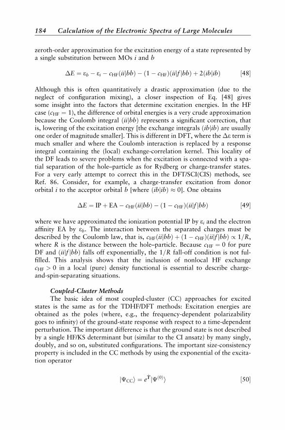
zeroth-order approximation for the excitation energy of a state represented bya single substitution between MOs i and b

�E ¼ eb � ei � cHFðiijbbÞ � ð1� cHFÞðiijf jbbÞ þ 2ðibjibÞ ½48

Although this is often quantitatively a drastic approximation (due to theneglect of configuration mixing), a closer inspection of Eq. [48] givessome insight into the factors that determine excitation energies. In the HFcase (cHF ¼ 1), the difference of orbital energies is a very crude approximationbecause the Coulomb integral ðiijbbÞ represents a significant correction, thatis, lowering of the excitation energy [the exchange integrals ðibjibÞ are usuallyone order of magnitude smaller]. This is different in DFT, where the �e term ismuch smaller and where the Coulomb interaction is replaced by a responseintegral containing the (local) exchange-correlation kernel. This locality ofthe DF leads to severe problems when the excitation is connected with a spa-tial separation of the hole–particle as for Rydberg or charge-transfer states.For a very early attempt to correct this in the DFT/SCI(CIS) methods, seeRef. 86. Consider, for example, a charge-transfer excitation from donororbital i to the acceptor orbital b [where ðibjibÞ � 0]. One obtains

�E ¼ IPþ EA� cHFðiijbbÞ � ð1� cHFÞðiijf jbbÞ ½49

where we have approximated the ionization potential IP by ei and the electronaffinity EA by eb. The interaction between the separated charges must bedescribed by the Coulomb law, that is, cHFðiijbbÞ þ ð1� cHFÞðiijf jbbÞ / 1=R,where R is the distance between the hole–particle. Because cHF ¼ 0 for pureDF and ðiijf jbbÞ falls off exponentially, the 1=R fall-off condition is not ful-filled. This analysis shows that the inclusion of nonlocal HF exchangecHF > 0 in a local (pure) density functional is essential to describe charge-and-spin-separating situations.

Coupled-Cluster MethodsThe basic idea of most coupled-cluster (CC) approaches for excited

states is the same as for the TDHF/DFT methods: Excitation energies areobtained as the poles (where, e.g., the frequency-dependent polarizabilitygoes to infinity) of the ground-state response with respect to a time-dependentperturbation. The important difference is that the ground state is not describedby a single HF/KS determinant but (similar to the CI ansatz) by many singly,doubly, and so on, substituted configurations. The important size-consistencyproperty is included in the CC methods by using the exponential of the excita-tion operator

j�CCi ¼ eTT j�ð0Þi ½50


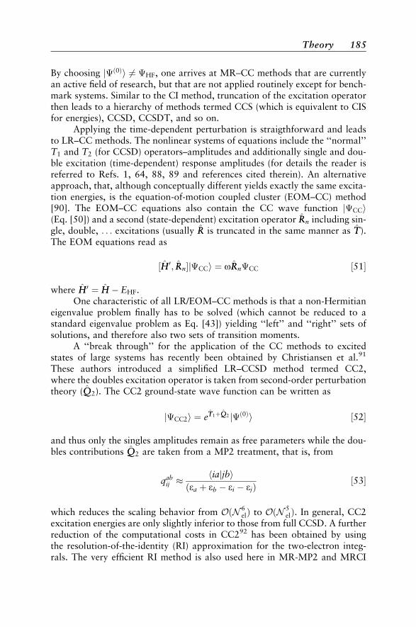
By choosing j�ð0Þi 6¼ �HF, one arrives at MR–CC methods that are currentlyan active field of research, but that are not applied routinely except for bench-mark systems. Similar to the CI method, truncation of the excitation operatorthen leads to a hierarchy of methods termed CCS (which is equivalent to CISfor energies), CCSD, CCSDT, and so on.

Applying the time-dependent perturbation is straigthforward and leadsto LR–CC methods. The nonlinear systems of equations include the ‘‘normal’’T1 and T2 (for CCSD) operators–amplitudes and additionally single and dou-ble excitation (time-dependent) response amplitudes (for details the reader isreferred to Refs. 1, 64, 88, 89 and references cited therein). An alternativeapproach, that, although conceptually different yields exactly the same excita-tion energies, is the equation-of-motion coupled cluster (EOM–CC) method[90]. The EOM–CC equations also contain the CC wave function j�CCi(Eq. [50]) and a second (state-dependent) excitation operator RRn including sin-gle, double, . . . excitations (usually RR is truncated in the same manner as TT).The EOM equations read as

½HH0; RRnj�CCi ¼ oRRn�CC ½51

where HH0 ¼ HH � EHF.One characteristic of all LR/EOM–CC methods is that a non-Hermitian

eigenvalue problem finally has to be solved (which cannot be reduced to astandard eigenvalue problem as Eq. [43]) yielding ‘‘left’’ and ‘‘right’’ sets ofsolutions, and therefore also two sets of transition moments.

A ‘‘break through’’ for the application of the CC methods to excitedstates of large systems has recently been obtained by Christiansen et al.91

These authors introduced a simplified LR–CCSD method termed CC2,where the doubles excitation operator is taken from second-order perturbationtheory (QQ2). The CC2 ground-state wave function can be written as

j�CC2i ¼ eTT1þQQ2 j�ð0Þi ½52

and thus only the singles amplitudes remain as free parameters while the dou-bles contributions QQ2 are taken from a MP2 treatment, that is, from

qabij �

hiajjbiðea þ eb � ei � ejÞ

½53

which reduces the scaling behavior from OðN 6elÞ to OðN 5

elÞ. In general, CC2excitation energies are only slightly inferior to those from full CCSD. A furtherreduction of the computational costs in CC292 has been obtained by usingthe resolution-of-the-identity (RI) approximation for the two-electron integ-rals. The very efficient RI method is also used here in MR-MP2 and MRCI

Theory 185

methods as described before [66, 78]. The error for the excitation energiesintroduced by the RI approach is �0.01–0.03 eV, which is clearly insignificantcompared to other sources of error like basis set truncation error that is of theorder of 0.1–0.2 eV with standard cc-pVTZ basis sets. An analytical gradientfor RI-CC2 has also been reported recently,93 which routinely allows for geo-metry optimizations of medium-sized molecules. This recent advance includesa significant fraction of dynamical electron correlation (as opposed to CIS andCASSCF that have hitherto been frequently used for that purpose).

RecommendationsHere, we provide a summary of the quantum chemical methods that can,

and should be applied to the calculation of electronic spectra of large systems:

1. Hartree–Fock based methods (TDHF and CIS): Good energetic results fromthese methods cannot be obtained; the errors for excitation energies oftenexceed 0.5 eV. For low-spin states, �E is often too large so scaling factorsof �0.7–0.8 are in use while the �E values for high-spin states are usuallyunderestimated. Contrary to statements in the literature,94 the results areoften even qualitatively wrong (false state ordering). The Rydberg states,for which they appear to perform reasonably well, are not really importantfor large systems. Because excited-state geometries are relatively insensitiveto correlation effects, these methods may be used (after careful calibration)for that purpose but even this is difficult because the predicted order ofstates is often wrong. Both TDHF and CIS methods have a tendency (asdoes HF for ground states) to break symmetry, and consequently they oftenyield geometries that are too distorted. They are to be preferred overTDDFT if the asymptotic behavior of the potential (see below) is of crucialimportance. They are sometimes applicable if only relative trends in a seriesof very similar molecules are of interest.

2. Coupled-cluster methods: For systems with well-behaved ground states,and, if the excited states are reasonably described by single excitations,low-order coupled cluster methods (CC291 or LR/EOM-CCSD64, 90) canprovide good accuracy (errors < 0.3 eV). Especially when used togetherwith efficient integral approximations (RI-CC292) computations can beperformed for fairly large molecules. For more complicated excited statesor when the ground state is already strongly correlated, the inclusion of TT3

is mandatory, which limits the applicability to small molecules.3 Perturbation methods: In general, second-order multireference PT methods

can be recommended for excited-state problems. They usually show verygood accuracy (errors < 0.2 eV, excitation energies are systematicallyunderestimated) and they can be applied to a wide variety of states andproblems. However, MRPT methods are not ‘‘black-box’’ and carefulchecks of the technical details like the size of reference space, choice oforbitals, and so on, must be done. These methods require a lot of user


experience, as well as detailed insight into the system. For many states inthe high-energy regions, the reference wave functions become prohibitivelylarge, and, the second-order treatment often breaks down. The most seriousdisadvantage is that the results are very sensitive to the so-called ‘‘intruderstates’’, which have low zeroth-order energies but are only weaklyinteracting with the reference state.

4. Density functional methods: The TDDFT approaches employing hybridfunctionals such as B3LYP20,21 or BHLYP95 are always the method ofchoice for providing a first overview about the electronic spectrum of aparticular molecule. The errors for �E are much smaller than with TDHF/CIS and usually within 0.3–0.4 eV of experiment (often �E is under-estimated). For larger transition metal compounds, TDDFT is the onlymethod that is routinely applicable. The same holds for spectra, where onthe order of a hundred different states must be considered. With common(asymptotically incorrect) functionals, larger errors are obtained forRydberg85,96 (see the following section) and charge-transfer states97–99 orfor states with strong contributions from ionic valence-bond structures.35 Acalibration on ab initio or experimental data and a check of the functionaldependence of the results is strongly recommended.

5. Basis sets: The basis set requirements in excited-state applications are notvery different than those for the corresponding ground state if only low-lying valence states are considered, and thus, properly polarized valence-triple-� (or even double-�) sets are often good enough (i.e., they provide �Eto within 0.1 eV). Because the valence excited states of medium-sizedsystems can sometimes include diffuse components, a check of, forexample, the r2

�expectation values (see the following section) is

recommended and depending on its value, diffuse basis functions must beadded (for an example, see a later section). For low-lying Rydberg states,additional atom-centered diffuse sets of single-� quality ([1s1p1d]/[1s1p]for main group compounds) are sufficient.

6. Semiempirical approaches represent an alternative quantum chemicalmethod especially for very large systems or when only main groupcompounds without complicated electronic structure are involved. As forthe ground states, however, they are gradually being displaced by the moreaccurate and robust DFT methods. Of the many semiempirical approaches,the all-valence methods with orthogonalization corrections100,101 and thesimplest Pariser–Parr–Pople (PPP) type methods for very large p-systemscan be recommended (for a recent application to a 600 atom system, seeRef. 102). One area of application is the prediction of excited-stategeometries where MNDO/CI approaches seem to be quite successful.103,104

For excitation energies, however, standard MNDO, AM1, or PM3Hamiltonians employing small CI expansions show large systematic aswell as unpredictable (random) errors. Careful calibration is thusmandatory with all semiempirical methods.

Theory 187

CASE STUDIES

Vertical Absorption Spectra

AcetoneIn this section, some general aspects of the computation of Rydberg spec-

tra are discussed (for reviews on this topic, see Ref. 6 and Ref. 105; for a recenttheoretical study on very high-lying Rydberg states (which will not be consid-ered here), see Ref. 106). Although Rydberg states are ubiquitous, they are oflesser importance in the spectra of large molecules that are dominated byvalence states. The reason to begin this section with this topic is twofold: First,Rydberg states are mostly of relatively simple structure, being dominated by afew (mostly one) single excitations and are thus easy to understand intuitivelyin a MO picture. Second, the excitation process is accompanied with a spatialseparation of the electrons that is typical also for some valence states. Thisleads to problems with most density functionals as already discussed in anearlier section.

The transitions to Rydberg states generally have low intensities becauseof the large spatial extension of the final orbital (small overlap with the originorbital yields weak transition densities) and consequently they are often hid-den under more intense valence bands. As an example, here we therefore haveto investigate a small molecule where the valence transitions are spectrallyseparated. Saturated ketones show only two valence states, namely, then! p� state at �4 eV and a very high-lying p! p� state so that a numberof Rydberg transitions can be observed in the 6–9-eV range. Acetone, the sim-plest aliphatic ketone, is probably the best experimentally studied moleculeof this group of important organic systems. Of the few theoretical studiesthat exist, we mention here only the most recent CASPT2 work of Merchanet al.,107 where key references to the experimental data and older theoreticalwork can also be found.

Figure 10 shows the two orbitals that are involved in the first n! 3sRydberg transition of acetone. The very different spatial extensions are clearlyvisible and especially in the outer regions of the 3s MO its almost sphericalcharacter can be seen.

The distinction between Rydberg and valence states is not that clear inlarger molecules. A good indicator for the state character can be obtained fromthe hr 2i expectation value (a measure of spatial extension) difference for staten with respect to the ground state. This is given by

� r 2 �

¼ �n jrr 2j�n

�� 0jrr 2j�0

�½54

where

rr 2 ¼ xx2 þ yy2 þ zz2 ½55


is the trace of the Cartesian electric quadrupole operator. For molecules com-posed of second-row atoms, the � r 2

�values are usually in the range 30–50

(3s), 50–100 (3p), and > 100 a20 for 3d states, respectively, while they are

usually < 10 a20 for pure valence states.

The ‘‘diffuseness’’ of Rydberg states leads to complications with somequantum chemical approaches. When using MRCI or MRPT2 methods it isabsolutely necessary to use virtual orbitals that are optimized in the presenceof the correct potential of Nel � 1 electrons. The (closed-shell) HF potential forthe virtual orbitals includes the (nuclear charge) shielding of all Nel electronsand thus the Rydberg part of the spectrum is too diffuse, which leads to arti-ficial configuration mixing in the CI procedures (to a lesser extent, however,this also holds for some valence states, especially for medium-sized systems).Experience shows that individually optimized orbitals are not necessary, butinstead, ROHF orbitals of, for example, the lowest cation state, can beemployed.

The problems of most density functionals with Rydberg states are alsorelated to the electronic potential far away from the nuclei. It is well knownthat the local density approximation (LDA) exchange potential vLDA

X / rðrÞ1=3

Figure 10 Contour plots of the lone-pair MO (a) and 3s Rydberg MO (b) for acetone inthe O��CCC plane. Because of the too high potential for the virtual orbitals in ground-state HF treatments, the calculations refer to a ROHF/d-aug-cc-pVDZ treatment for the2B2 cation ground state.

Case Studies 189

decays asymptotically exponentially with r [as the density rðrÞ itself] instead ofwith 1=rþ const. This behavior, which can also be explained by the artificialelectron self-interaction, leads to (a) too small electron binding, that is, toolow Rydberg excitation energies and to (b) a too fast approach of the asymp-totic (ionized) limit. Figure 11 shows the �E values for the 2p! ns (n ¼ 3--7,n indicates the principal quantum number) Rydberg series of the neon atom ascalculated with TDHF and various TDDFT methods.

It is seen that while the TDHF results are just shifted with respect to theexperimental data, the shape of the �E versus n curves is qualitatively wrongwith the TDDFT methods. With a pure DF completely lacking ‘‘exact’’ HFexchange (e.g., BP86108, 109) there is not only a large underestimation of the�E values, but furthermore almost no dependence on n up to n ¼ 6 and afterthat even a strong energy increase is clearly visible. As expected, the situationis gradually improved by ‘‘exact’’ exchange mixing (from 20% in B3LYP to50% in BHLYP95) and only the latter functional can be recommended forthe computation of Rydberg spectra. The construction of a DF with the correctasymptotic behavior is currently an active field of research (for details andpossible solutions to the problem see Refs. 96, 110, 111 and references citedtherein).

This behavior of the DF is also observed in molecular applications.Vertical singlet excitation energies from CASPT2107, TDDFT-B3LYP, and

3 4 5 6 72p>ns

12

13

14

15

16

17

18

19

20

21

22

23

24

25

∆E (

eV)

HFBHLYPB3LYPBPexp.

1.IP(exp.)

Figure 11 Excitation energies for the singlet 2p! nsðn ¼ 3--7Þ Rydberg series of theneon atom (½6s4p þ 8s AO basis).


MRCI computations (d-aug-cc-pVDZ AO basis, B3LYP/TZV(d,p) ground-state geometry) are compared with experimental data in Table 5. A graphicalcomparison with an experimental gas-phase absorption spectrum is shown inFigure 12.

The underestimation of the �E values with TDDFT increases from�0.65 eV for the n! 3s transition to > 1 eV for the n! 3d states. The

Table 5. Calculated and Experimental Excitation Energies (in eV) and OtherProperties of the Vertical Singlet Excited States of Acetone

�E——————————————————————

State B3LYP CASPT2a MRCI Exp.a f L � r2 �

1B2ðn! 3sÞ 5.71 6.58 6.51 6.35 0.037 46.22A2ðn! 3pxÞ 6.61 7.34 7.41 7.36 75.72A1ðn! 3pyÞ 6.50 7.26 7.44 7.41 0.006 90.72B2ðn! 3pzÞ 6.66 7.48 7.49 7.45 0.002 85.63A1ðn! 3dyzÞ 7.12 7.91 8.14 7.80 0.047 123.03B2ðn! 3dx2�y2Þ 6.93 8.04 7.92 8.09 0.048 109.73A2ðn! 3dxzÞ 7.24 8.09 8.17 118.04B2ðn! 3dz2Þ 7.18 8.18 8.21 0.004 133.31B1ðn! 3dxyÞ 7.17 8.20 8.25 8.17 0.002 131.1

aRef. 107.

6 6.5 7 7.5 8 8.5∆E (eV)

0

0.2

0.4

0.6

0.8

1

rela

tive

inte

nsity

exp.TDDFT/B3LYP MRCI

0.03

0.02

0.01

0.04

0.05

n3s

n3p

n3d

osci

llato

r st

reng

th

Figure 12 Comparison of the experimental UV spectrum of acetone112 with calculatedvertical transitions. The theoretical �E values are shifted by�0.15 (MRCI) and 0.65 eV(TDDFT), respectively.

Case Studies 191

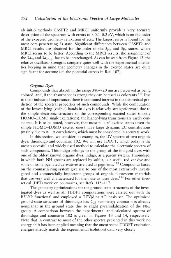
ab initio methods CASPT2 and MRCI uniformly provide a very accuratedescription of the spectrum with errors of �0.1–0.2 eV, which is on the orderof the expected geometry relaxation effects. The largest error is found for themost core-penetrating 3s state. Significant differences between CASPT2 andMRCI results are obtained for the order of the 3px and 3py states, whereMRCI seems to be better. According to the MRCI results, the assignment ofthe 3dyz and 3dx2�y2 has to be interchanged. As can be seen from Figure 12, therelative oscillator strengths compare quite well with the experimental intensi-ties keeping in mind that geometry changes in the excited states are quitesignificant for acetone (cf. the potential curves in Ref. 107).

Organic DyesCompounds that absorb in the range 380–720 nm are perceived as being

colored, and, if the absorbance is strong they can be used as colorants.113 Dueto their industrial importance, there is continued interest in the theoretical pre-diction of the spectral properties of such compounds. While the computationof the lowest-lying (visible) bands in dyes is relatively straightforward due tothe simple electronic structure of the corresponding excited states (mostlyHOMO–LUMO single excitations), the higher-lying transitions are rarely con-sidered. It is to be noted, however, that most p! p� excited states (even thesimple HOMO–LUMO excited ones) have large dynamic EC contributions(mainly due to s� p correlation), which must be considered in accurate work.

In this section, we consider, as examples, the UV spectra of two organicdyes: thioindigo and coumarin 102. We will use TDDFT, which today is themost successful and widely used method to calculate the electronic spectra ofsuch compounds. Thioindigo belongs to the group of the indigoid dyes withone of the oldest known organic dyes, indigo, as a parent system. Thioindigo,in which both NH groups are replaced by sulfur, is a useful red vat dye andsome of its halogenated derivatives are used as pigments.113 Compounds basedon the coumarin ring system give rise to one of the most extensively investi-gated and commercially important groups of organic fluorescent materialsthat are very well characterized for their use as laser dyes.114 For other theo-retical (DFT) work on coumarins, see Refs. 115–117.

The geometry optimizations for the ground-state structures of the inves-tigated dyes as well as all TDDFT computations were carried out with theB3LYP functional and employed a TZV(d,p) AO basis set. The optimizedground-state structure of thioindigo has C2h symmetry; coumarin is alreadynonplanar in the ground state due to slight pyramidalization of the NR2

group. A comparison between the experimental and calculated spectra ofthioindigo and coumarin 102 is given in Figures 13 and 14, respectively.Note that in contrast to most of the other spectra presented in this work noenergy shift has been applied meaning that the uncorrected TDDFT excitationenergies already match the experimental (solution) data very closely.


Figure 13 Comparison of experimental and computed [B3LYP/TZV(d,p)] UV spectraof thioindigo.

Figure 14 Comparison of experimental and computed [B3LYP/TZV(d,p)] UV spectraof coumarin 102.

Case Studies 193

The visible and near-UV spectrum of thioindigo measured in benzeneshow two major bands with maxima at �2.3 and 4.2 eV,118 respectively.The calculated lowest excitation energy and oscillator strengths, which arearguably of most interest to the dye chemist, are in excellent agreement withthe experimental values. The lowest lying 11Bu state computed at 2.36 eV is ofp! p� character and results mainly from the HOMO ! LUMO excitation.Despite this simple electronic structure, the (dynamical) EC contributions arelarge as can be seen by comparison with the TDHF excitation energy (3.77eV), which is in error by > 1.4 eV. The second feature observed in the UVspectrum of thioindigo is a relatively broad absorption including twoshoulders at 3.7 and 4.1 eV. Our calculations show that in this energy regionthere are two 1Bu transitions close in energy: The 21Bu computed at 3.84 eVand the 31Bu at 4.06 eV. Both states have purely p! p� character and resultmainly from HOMO-3!LUMO and HOMO-6!LUMO excitations, respec-tively. The almost perfect agreement between the experimental and calculatedspectral data demonstrates that TDDFT provides a very reliable description ofhigher-lying valence states.

The experimental absorption spectrum of coumarin 102 obtained inethanol solution exhibits two intense absorption bands at 3.2 and 5.9 eVand one band with a lower intensity located at �4.8 eV.114 As for thioindigo,the lowest-lying state is of p! p� type and mainly results from the HOMO!LUMO excitation. The third state calculated at 4.50 eV with small intensityðf ¼ 0:085Þ is due to the two nearly degenerate configurations HOMO-1!LUMO and HOMO! LUMOþ 1 and assigned to the band located inthe experimental spectrum at 4.8 eV. The third band in the spectrum of cou-marin 102 is relatively broad with a maximum �5.9 eV. According tothe TDDFT calculations, this band is composed mainly of two transitions tothe 10A and 11A states calculated at 5.85 and 6.02 eV, respectively. In thiscase, we observe some overestimation of the calculated intensities that maybe caused by solvent effects. Note, however, that TDDFT errors of �50%for oscillator strengths, especially for higher-lying transitions, are not unusualand that the neglected vibronic effects (FC factors much smaller than unity)may also contribute to this error.

Transition Metal ComplexesDescribing the electronic structure of transition metal compounds

remains a challenging goal in quantum chemistry in general. The importanceof static correlation effects arising from near degeneracy within the metal d-shells causes difficulties in ab initio single-reference treatments (in TDDFTthere is some implicit account of static EC). Additionally, the low quality ofthe Hartree–Fock orbitals for transition metal compounds complicates theapplication of approaches lacking appropriate orbital relaxation effects.The TDDFT method is currently the only one that can be applied routinelyto these systems, especially when large compounds without any symmetry


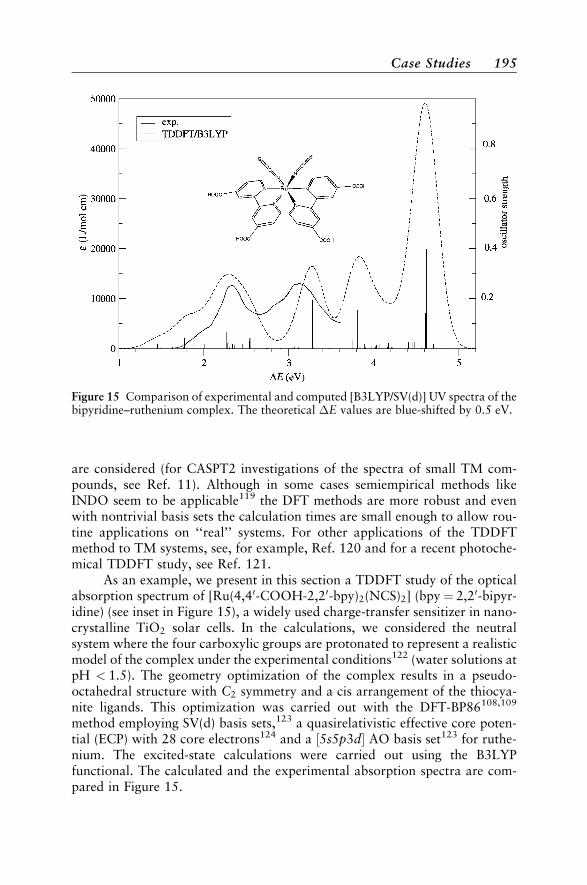
are considered (for CASPT2 investigations of the spectra of small TM com-pounds, see Ref. 11). Although in some cases semiempirical methods likeINDO seem to be applicable119 the DFT methods are more robust and evenwith nontrivial basis sets the calculation times are small enough to allow rou-tine applications on ‘‘real’’ systems. For other applications of the TDDFTmethod to TM systems, see, for example, Ref. 120 and for a recent photoche-mical TDDFT study, see Ref. 121.

As an example, we present in this section a TDDFT study of the opticalabsorption spectrum of [Ru(4,40-COOH-2,20-bpy)2(NCS)2] (bpy¼ 2,20-bipyr-idine) (see inset in Figure 15), a widely used charge-transfer sensitizer in nano-crystalline TiO2 solar cells. In the calculations, we considered the neutralsystem where the four carboxylic groups are protonated to represent a realisticmodel of the complex under the experimental conditions122 (water solutions atpH < 1.5). The geometry optimization of the complex results in a pseudo-octahedral structure with C2 symmetry and a cis arrangement of the thiocya-nite ligands. This optimization was carried out with the DFT-BP86108,109

method employing SV(d) basis sets,123 a quasirelativistic effective core poten-tial (ECP) with 28 core electrons124 and a ½5s5p3d AO basis set123 for ruthe-nium. The excited-state calculations were carried out using the B3LYPfunctional. The calculated and the experimental absorption spectra are com-pared in Figure 15.

Figure 15 Comparison of experimental and computed [B3LYP/SV(d)] UV spectra of thebipyridine–ruthenium complex. The theoretical �E values are blue-shifted by 0.5 eV.

Case Studies 195

The experimental spectrum exhibits two bands in the visible and near-UV region centered at 2.3 and 3.1 eV,125 respectively. The overall band shapesand their relative and absolute intensities are well described by the TDDFTapproach and even the shoulder at �1.9 eV is predicted correctly. The under-estimation of the calculated excitation energies by �0.5 eV may on the onehand be attributed to inabilities of the chosen density functional but on theother hand certainly includes solvation effects that have been studied in Ref.126 in the framework of continuum models. The neglected effects of spin–orbit coupling may be on the order of 0.1–0.2 eV, which seems to be signifi-cantly smaller than the differences obtained with various density functionals.As can be seen by the vertical lines included in Figure 15, which indicate theposition and f values of the individual transitions, the density of electronictransitions even in the low-energy range is quite high. For the first two bands,�25 electronic states have to be considered, which increases to �60 in therange up to 5 eV. The TDDFT method is the only one that is currently applic-able in such situations.

The character of the electronic transitions is usually analyzed in terms ofthe contributing single excitations. Although this is sometimes problematicdue to extensive orbital and configuration mixing, the analysis is straightfor-ward in our particular example. The first absorption band has strong multi-configurational character and involves excitations from the highest occupiedto the lowest unoccupied p� molecular orbitals. The many orbitals close tothe HOMO are mainly of ruthenium d-orbital character with significantamplitudes on the isothiocyanate ligands. The second and the third absorptionband involve excitations from a second set of metal d orbitals, to the lowestunoccupied p� molecular orbitals, which can be characterized as metal–ligandcharge-transfer (MLCT) bands. The fourth band at�4.6 eV is very intense andcan easily be assigned to intraligand (p! p�) excitations.

Open-Shell Systems: The Phenoxyl RadicalDue to its crucial role in combustion chemistry and biology, the phenoxyl

radical has been the subject of intense experimental and theoretical studies formany years (for recent work, see Ref. 127 and references cited therein). Forthese reasons we present it here as an example of UV spectroscopy of (neutral)radicals (for the application of DFT to the spectra of aromatic radical cations,see, e.g., Ref. 128 and for results of MRCI computations, see Ref. 129). Thephenoxyl radical is well known as a difficult case for electronic structuremethods because it requires a sophisticated treatment of electron correlationsimilar to closed-shell aromatic hydrocarbons.

In agreement with previous DFT studies,127 we found a 2B1 ground state(assuming C2v symmetry with yz being the molecular plane) corresponding toa singly occupied orbital (SOMO) of p type. The lowest excited state corre-sponds to a n! p(D-S) transition of B2 symmetry, which is dipole-forbidden.A weak band observed experimentally at �1.1 eV (1120 nm) supports this


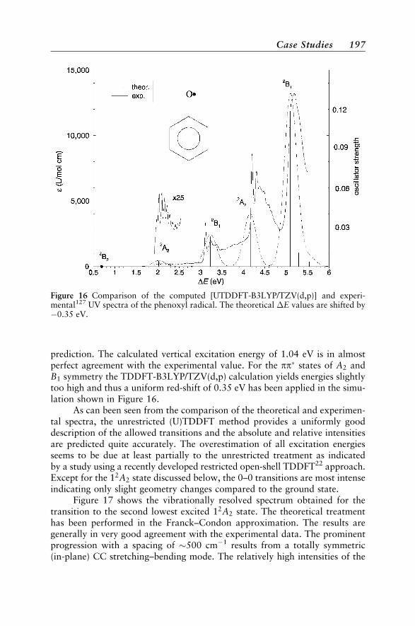
prediction. The calculated vertical excitation energy of 1.04 eV is in almostperfect agreement with the experimental value. For the pp� states of A2 andB1 symmetry the TDDFT-B3LYP/TZV(d,p) calculation yields energies slightlytoo high and thus a uniform red-shift of 0.35 eV has been applied in the simu-lation shown in Figure 16.

As can been seen from the comparison of the theoretical and experimen-tal spectra, the unrestricted (U)TDDFT method provides a uniformly gooddescription of the allowed transitions and the absolute and relative intensitiesare predicted quite accurately. The overestimation of all excitation energiesseems to be due at least partially to the unrestricted treatment as indicatedby a study using a recently developed restricted open-shell TDDFT22 approach.Except for the 12A2 state discussed below, the 0–0 transitions are most intenseindicating only slight geometry changes compared to the ground state.

Figure 17 shows the vibrationally resolved spectrum obtained for thetransition to the second lowest excited 12A2 state. The theoretical treatmenthas been performed in the Franck–Condon approximation. The results aregenerally in very good agreement with the experimental data. The prominentprogression with a spacing of �500 cm�1 results from a totally symmetric(in-plane) CC stretching–bending mode. The relatively high intensities of the

Figure 16 Comparison of the computed [UTDDFT-B3LYP/TZV(d,p)] and experi-mental127 UV spectra of the phenoxyl radical. The theoretical �E values are shifted by�0.35 eV.

Case Studies 197

0–1, 0–2, and 0–3 vibrational transitions can be explained by the geometriesof the phenoxyl radical in the ground and excited states and the nature of thenormal modes. The X2B1 ground state has a partially chinoid structure withshort C��O (1.25 A) and C2–C3/C5–C6 (1.37 A) bond lengths. The C��Cbonds elongate in the 12A2 state to �1.43 A, thus matching almost exactlythe geometric changes induced by the above mentioned stretching–bendingmode. This example clearly shows how a vibrational analysis can reveal struc-tural details of the corresponding states. Further examples of this type will bediscussed in a later section.

Open–Shell Systems: Excited-State Absorption of NaphthaleneExcited-state absorption (ESA) is a type of electronic spectroscopy for

which only a few theoretical studies have been performed (for a recent studyon the singlet–singlet ESA spectrum of azulene, see Ref. 130 and for somebenchmark calculations on small molecules, see Ref. 131). From the experi-mental point of view ESA is a very important topic in photophysical (kinetic)investigations of energy, electron or hydrogen-transfer processes. Although inprinciple all excited states of a molecule show a distinct electronic absorptionspectrum, only the ESA spectra of the lowest excited state in each multiplicity(i.e., S1 or T1) are usually accessible experimentally. Because of the short

Figure 17 Comparison of the computed [UTDDFT-B3LYP/TZV(d,p)] and experi-mental127 UV band of the 12A2 state of the phenoxyl radical. The 0–0 transition energyis set to zero.


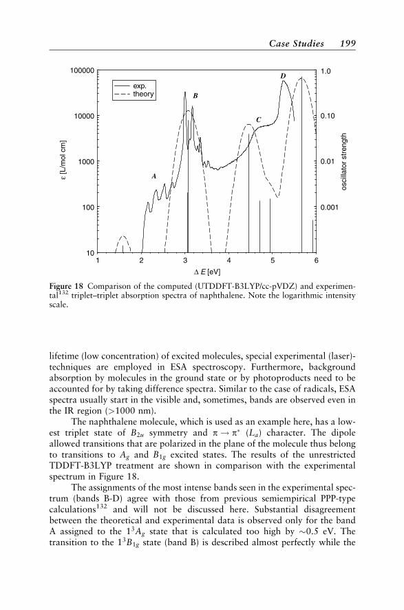
lifetime (low concentration) of excited molecules, special experimental (laser)-techniques are employed in ESA spectroscopy. Furthermore, backgroundabsorption by molecules in the ground state or by photoproducts need to beaccounted for by taking difference spectra. Similar to the case of radicals, ESAspectra usually start in the visible and, sometimes, bands are observed even inthe IR region (>1000 nm).

The naphthalene molecule, which is used as an example here, has a low-est triplet state of B2u symmetry and p! p� (La) character. The dipoleallowed transitions that are polarized in the plane of the molecule thus belongto transitions to Ag and B1g excited states. The results of the unrestrictedTDDFT-B3LYP treatment are shown in comparison with the experimentalspectrum in Figure 18.

The assignments of the most intense bands seen in the experimental spec-trum (bands B-D) agree with those from previous semiempirical PPP-typecalculations132 and will not be discussed here. Substantial disagreementbetween the theoretical and experimental data is observed only for the bandA assigned to the 13Ag state that is calculated too high by �0.5 eV. Thetransition to the 13B1g state (band B) is described almost perfectly while the

1 2 3 4 5 6

∆ E [eV]

10

100

1000

10000

100000ε

[L/m

ol c

m]

exp.theory

0.01

0.001

osci

llato

r st

reng

th

0.10

1.0

A

B

C

D

Figure 18 Comparison of the computed (UTDDFT-B3LYP/cc-pVDZ) and experimen-tal132 triplet–triplet absorption spectra of naphthalene. Note the logarithmic intensityscale.

Case Studies 199

predicted excitation energies for band C and D show the typical TDDFT errorson the order of �0.2–0.4 eV. Note, however, that the relative description forthe different states is worse compared to the phenoxyl radical where a globalshift of all excitation energies yields a satisfactory agreement with experiment.This is because of the more complicated electronic structure of the naphtha-lene T1 state (two vs. one open shell for the phenoxyl radical), which seemsnot to be described well enough by the simple TDDFT treatment. Further-more, due to technical limitations it is currently not possible to check thedegree of spin-contamination of the excited states (hSS2i expectation value).Conclusive answers about the applicability of TDDFT in this area of spectro-scopy requires more detailed work on other systems.

Circular Dichroism

2,3-(S,S)-DithiadecalinThe nature of the chromophore of a molecule has a major influence on

the corresponding CD spectroscopic properties. If the chromophore itself ischiral, it is denoted as being ‘‘inherently chiral’’, whereas the term ‘‘inherentlyachiral’’ is used for locally achiral chromophores that are disturbed by theirchiral surrounding (for a more detailed classification, see Ref. 133). Thestrength of the Cotton effect (rotatory strengths) provided by molecules con-taining an inherently chiral chromophore usually exceeds what is found for amolecule containing an inherently achiral chromophore by an order of magnitude.

The dithiadecalin (DTD) molecule (see inset in Figure 19) is character-ized by the local chiral disulfide chromophore. Its first two transitions areexpected to be of valence character and can be understood as single excitationsout of the lone-pair orbitals at the sulfur atoms into the corresponding sðSSÞ�orbital. However, the �hr 2i values of the transitions indicate significantlymore diffuse character than expected for pure valence excited states.

To account for this fact, the TDDFT-B3LYP calculations of the spectrahave been carried out with a TZV(2df) basis set augmented with diffuse func-tions at the sulfur atoms as well as at the neighboring carbon atoms and aTZV(d,p) basis set for the remaining atoms. The B3LYP/TZV(d,p) ground-state geometry has been used for these calculations. The theoretical spectrumhas been blue shifted by 0.39 eV to match the experimental band A.

The experimental spectra of DTD134 have been recorded in hexane.Keeping in mind the above described diffuse character of all excited statesin DTD, an unbalanced theoretical description of states with stronger Rydbergcharacter is to be expected when gas-phase data are compared with those fromthe condensed phase (Pauli-repulsion between the Rydberg state and solventmolecule wave functions). Figure 19, however, shows an almost perfect matchbetween the theoretical gas-phase and experimental CD spectrum in the entireenergy range. Even band C, which is theoretically predicted to have almost


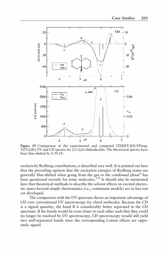
exclusively Rydberg contributions, is described very well. It is pointed out herethat the prevailing opinion that the excitation energies of Rydberg states aregenerally blue-shifted when going from the gas to the condensed phase6 hasbeen questioned recently for some molecules.135 It should also be mentionedhere that theoretical methods to describe the solvent effects on excited electro-nic states beyond simple electrostatics (i.e., continuum models) are in fact notyet developed.

The comparison with the UV spectrum shows an important advantage ofCD over conventional UV spectroscopy for chiral molecules. Because the CDis a signed quantity, the band B is considerably better separated in the CDspectrum. If the bands would lie even closer to each other such that they couldno longer be resolved by UV spectroscopy, CD spectroscopy would still yieldtwo well-separated bands since the corresponding Cotton effects are oppo-sitely signed.

Figure 19 Comparison of the experimental and computed [TDDFT-B3LYP/aug-TZV(2df)] UV and CD spectra for 2,3-(S,S)-dithiadecalin. The theoretical spectra havebeen blue-shifted by 0.39 eV.

Case Studies 201

(M)-[6]HeliceneHexahelicene is one of the most widely studied molecules in theoretical

CD spectroscopy (see, e.g., Refs. 47 and 136 and references cited therein). Thesystem is rather large [120 valence electrons, 590 basis functions with aTZV(d,p) AO basis] and �15–20 excited states are necessary to describe theexperimental spectrum entirely. This example is presented here to show thatcorrelated ab initio treatments are also applicable for such cases. The simpli-fied coupled-cluster model CC2 together with the RI approximation is usedand compared to the standard TDDFT-B3LYP approach.

The experimental CD spectrum (see Figure 20) consists of two veryintense CD bands with opposite sign at 5.1 eV (240 nm, F) and 3.8 eV (320nm, C). Shoulders (B, D, and E), and a very weak band (A) can, however, beclearly identified. With the exception of the region of band D, which is pre-dicted with the wrong CD sign in both calculations, the theoretical data arein good agreement with the experimental spectrum; that is to say, all bandshave a clear correspondence to calculated states. The theoretical excitationenergies from CC2 have been red-shifted by 0.22 eV, which is on the order

2.5 3 3.5 4 4.5 5 5.5∆ E [eV]

300

200

100

0

100

200

300

∆ε [l

/mol

cm

]

exp.theor. CC2theor. B3LYP

1/3

R [1

040 c

gs]

x10

A

B

C

D

E

F

Figure 20 Comparison of the experimental and computed [TZV(d,p) AO basis, B3LYPoptimized geometry] CD spectrafor (M)-[6]helicene. The theoretical spectra have beenshifted by 0.20 (B3LYP) and �0.22 eV (CC2), respectively. The filled circles/trianglesindicate the two lowest states with small intensity obtained by CC2/TDDFT-B3LYP.The vertical lines correspond to results from the CC2 method.


of the expected solvent effect. Further enlarging of the AO basis would bringthe CC2 data in even closer agreement with experiment (estimated effect of�0.1–0.2 eV). The TDDFT-B3LYP error is of opposite sign where the excita-tion energies are underestimated by �0.2 eV. The CC2 results are furthermoresuperior to those from TDDFT with respect to the splitting between the lowestLb (band A) and La (band B) states. The larger error for the high-energy bandF may be explained by some deficiencies of the TZV(d,p) AO basis set used,which lacks diffuse components as well as requisite higher angular momentumfunctions that are more important for explicitly correlated treatments than inDFT.

The computed intensities are also in reasonable agreement with experi-ment. The small R value for the Lb transition [�0:8� 10�40 cgs (CC2) vs.�1:6� 10�40 cgs (exp.)137] is predicted correctly with CC2 but has the wrongsign with TDDFT. However, this and the following La transition (band B) gainintensity by vibronic coupling with the close-lying intense Bb state and thus,results from vertical treatments should be taken cautiously.

When judging the accuracy of CC2 with respect to the TDDFT method,one should also consider the necessary computation times. While the TDDFTcalculation was completed in �15 hours (on a PIII/1.4-GHz machine), theCC2 treatment took >11 days, which corresponds to a timing ratio of �18.As mentioned before, the best strategy is thus to first calibrate the chosen den-sity functional(s) by comparison with ab initio approaches on smaller (butstructurally similar) molecules (in our example, e.g., ½3- or ½4helicene) andfinally to perform the calculation on the large target system using only thecheaper TDDFT method.

(2S)-Tricarbonyl-g4-pentadi-2,4-enal-ironAs mentioned in a previous section, the description of the electronic spectra of

transition metal compounds in low-oxidation states is relatively complicated.When applying DFT-based methods, it is recommended that one carefullyinvestigate the influence of the selected density functional. This is of particularimportance here because there are currently no ab initio methods on which theTDDFT approaches can be calibrated. As an example we present a study ofthe CD spectrum of (2S)-tricarbonyl-Z4-pentadi-2,4-enal-iron (ITP, for details,see Ref. 49). The molecule contains two achiral chromophores [pent-2,4-die-nal and the FeðCOÞ3 fragment] which, attached to each other, form the chiralsystem. The spectroscopic activity of ITP in the near-UV originates mainlyfrom 3dðmetalÞ ! p� excitations. As a result of the similar energies of severalelectronic configurations, extensive mixing is observed including variousn! p� states. Hence, it is understandable that the electronic nature of theexcited states in ITP is described very differently depending on which methodis applied. Furthermore, the energetic ordering and character of the MOs dif-fers substantially between Hartree–Fock based and DFT approaches as well asbetween different DFT functionals. A reasonable direct comparison of the

Case Studies 203

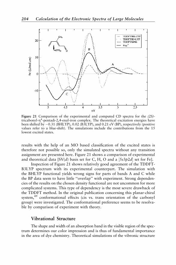
results with the help of an MO based classification of the excited states istherefore not possible so, only the simulated spectra without any transitionassignment are presented here. Figure 21 shows a comparison of experimentaland theoretical data [SV(d) basis set for C, H, O and a ½5s3p2d set for Fe].

Inspection of Figure 21 shows relatively good agreement of the TDDFT-B3LYP spectrum with its experimental counterpart. The simulation withthe BHLYP functional yields wrong signs for parts of bands A and C whilethe BP data seem to have little ‘‘overlap’’ with experiment. Strong dependen-cies of the results on the chosen density functional are not uncommon for morecomplicated systems. This type of dependency is the most severe drawback ofthe TDDFT method. In the original publication concerning this planar-chiralsystem,49 conformational effects (cis vs. trans orientation of the carbonylgroup) were investigated. The conformational preference seems to be resolva-ble by comparison of experiment with theory.

Vibrational Structure

The shape and width of an absorption band in the visible region of the spec-trum determines our color impression and is thus of fundamental importancein the area of dye chemistry. Theoretical simulations of the vibronic structure

Figure 21 Comparison of the experimental and computed CD spectra for the (2S)-tricabonyl-Z4-pentadi-2,4-enal-iron complex. The theoretical excitation energies havebeen shifted by �0.31 (BHLYP), 0.02 (B3LYP), and 0.21 eV (BP), respectively (positivevalues refer to a blue-shift). The simulations include the contributions from the 15lowest excited states.


of absorption bands allow us to evaluate the accuracy of the methods for find-ing the minimum energy geometries and vibrational frequencies. Systematicstudies of the vibrational structures of the absorption bands for large mole-cules have not been performed to date. A few investigations have been under-taken using semiempirical138 or CIS139 methods that however, did not givefully satisfactory results. For the first time, we will show here that reliable pre-dictions can be obtained in the framework of TDDFT. This has becomepossible due to the recently developed analytical TDDFT excited-stategradient.140 In fact, it will be shown that the excited-state geometries andvibrational frequencies from (TD)DFT are much more accurate than thecorresponding excitation energies (see also Ref. 141).

AnthraceneAs a first example, let us consider the vibronic structure of the first

absorption band in the UV spectrum of anthracene. In agreement with experi-ment, the TDDFT calculation gives an S1 state with B2u symmetry and a ver-tical excitation energy of 3.23 eV [�E0--0ðexp :Þ ¼ 3:43 eV]. This band can bedescribed by a HOMO! LUMO excitation and in the Platt nomenclature(perimeter model) it is denoted as the La state. Both states were optimizedat the (TD)DFT-B3LYP/TZV(d,p) level in D2h symmetry.

A comparison of the spectrum simulation with a low-resolution gas-phase absorption spectrum26 is shown in Figure 22. This type of spectrum is

Figure 22 Comparison of the computed [TDDFT-B3LYP/TZV(d,p)] and experimen-tal26 UV spectra for the 1La state of anthracene. The 0–0 transition energy is set to zero.

Case Studies 205

typical for large systems (normal UV spectra), and has therefore been chosenfor discussion here. The theoretical intensities were obtained within the FCapproximation at 0 K and the individual transitions were broadened by Gaus-sian shape functions using a half-width of s ¼ 165 cm�1.

The computed spectrum shows a good agreement with its experimentalcounterpart over the entire energy range. This indicates that the geometry andfrequency–normal mode changes between the two states are much betterdescribed by DFT than are the excitation energies (the DFT error for �E0--0

is �0.59 eV). The weak shoulders (hot-bands) located �300–750 cm�1 belowthe 0–0 transition cannot be described by the present calculation. Although thedescription of hot-bands is straightforward in principle (by thermal populationof vibrational ground-state levels), the current implementation of the recursiveintegral algorithm leads to unacceptably long computation times in such cases.As expected, the FC approximation seems to be very good for a dipole-allowedtransition as considered here. The gradual increase of the experimental inten-sity relative to the calculated one in Figure 22 may arise from a nonhorizontalbaseline in the measured spectrum. Furthermore, the second, less intense tran-sition to the S2 state (Lb) hidden under the La band may also contribute to thisintensity mismatch. All vibronic transitions with a high intensity correspond toexcitations of totally symmetric normal modes with a maximum excitation oftwo quanta in a single vibration.

OctatetracenePolyenes represent a class of widely studied molecules. Their ability to

undergo photochemical isomerizations is exploited by Nature to transduceradiative energy into chemical energy and thus, these systems perform vitalfunctions in many biochemical processes. All-trans octatetraene is used hereas a model system to assess the ability of DFT methods to predict the impor-tant spectroscopy of this and related systems.

A weak first absorption is found experimentally (�E0--0 ¼ 3:59 eV) cor-responding to the electric dipole-forbidden 1Ag ! 2Ag transition. The second(intense) band results from the allowed 1Ag ! 1Bu transition (�E0--0 ¼ 4:41eV). This situation is challenging for any theoretical method because the char-acter of both states is very different (single-configurational, ionic 1Bu state vs.multiconfigurational, covalent 2Ag state with significant contributions fromdouble excitations).

All calculations were performed at the (TD)DFT-B3LYP/TZV(d,p) levelemploying C2h symmetry. In contrast to the experimental data, the TDDFTcalculation yields an S1 state with Bu symmetry (�E0el ¼ 4:05 eV) and the2Ag state as the second one (�E0el ¼ 4:89 eV). This error can be traced tothe systematic underestimation of excitation energies for ionic states withTDDFT-B3LYP.35 Because of the adiabatic approximation used in theTDDFT treatments, the 2Ag state is described solely by a mixing ofHOMO! LUMOþ 1 and HOMO-1!LUMO single excitations. It lacks


the important HOMO–LUMO double excitation that has �30% weight inMR-MP2 wave functions. Thus we show here how such deficiencies of thetheoretical treatment transfer to the description of the geometries and vibra-tional frequencies, and finally to the simulated vibronic structure.

A comparison of computed (FC approximation, broadened by Lorent-zian functions with a half-width of s ¼ 20 cm�1) and experimental gas-phasespectra30 for the 1Bu state is shown in Figure 23. Compared to the previousexample, the theoretical description using B3LYP is worse. An obvious devia-tion from experiment is the relatively strong progression of the nontotallysymmetric normal mode with a frequency of 143 cm�1. This indicates an over-estimation of the frequency change for this mode upon electronic excitation.Because ionic p! p� states benefit from the inclusion of ‘‘exact’’ HFexchange,25 the calculation was repeated with the BHLYP functionalðEEX ¼ 50%Þ. As can be seen from Figure 23, this significantly improvesthe description of the vibronic structure that is now in acceptable agreementwith experiment over the entire energy range. Test calculations using TDHFðEEX ¼ 100%Þ yield results that deviate more strongly from experiment(not shown) indicating that there is some (state-dependent!) optimum ofexchange mixing in the density functionals.

Figure 23 Comparison of the computed [TDDFT/TZV(d,p)] and experimental30

spectra for the 1Bu state of octatetrene. The 0–0 transition energy is set to zero.

Case Studies 207

The dipole forbidden 1Ag ! 2Ag transition must be treated at the Herz-berg–Teller level (see earlier section) including the derivatives of the electronictransition dipole moment. These results are shown in Figure 24 in comparisonwith the experimental jet spectrum.31 The computed intensities were broad-ened with Lorentzian functions using a half-width of s ¼ 0:5 cm�1.

Somewhat surprisingly, the calculated spectrum shows an almost perfectagreement with the experiment. This seems to indicate that either the densityfunctional implicitly accounts for the missing double excitation (see also Ref.142) or that its influence on the shape of the excited-state potential energy sur-face is small or similar to that of the HOMO! LUMO þ 1 and HOMO�1! LUMO excitations. Based upon the intensity inducing bu mode with afrequency of 94 cm�1, which leads to mixing of the S1 and S2 states, severalexcitations of totally symmetric modes with low quantum numbers are observable.

FormaldehydeThe harmonic approximation is essential for computing the vibrational

structure of electronic bands for large molecules. For more ‘‘floppy’’ (low-energy) nuclear motions (like torsions and bendings), it is inadequate. Here,we present an example of how the harmonic treatment of such motions effectsthe shape of the calculated spectra. The electric dipole forbidden n! p�

Figure 24 Comparison of the computed [TDDFT-B3LYP/TZV(d,p)] and experimen-tal31 spectra for the 2Ag state of octatetraene. The 0–0 transition energy is set to zero.


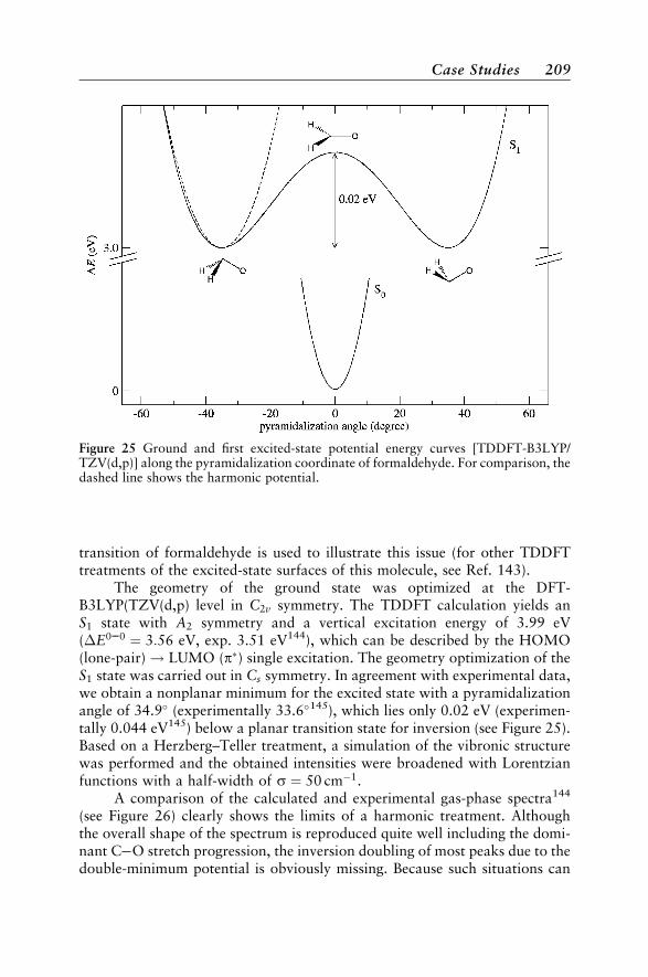
transition of formaldehyde is used to illustrate this issue (for other TDDFTtreatments of the excited-state surfaces of this molecule, see Ref. 143).

The geometry of the ground state was optimized at the DFT-B3LYP(TZV(d,p) level in C2v symmetry. The TDDFT calculation yields anS1 state with A2 symmetry and a vertical excitation energy of 3.99 eV(�E0--0 ¼ 3:56 eV, exp. 3.51 eV144), which can be described by the HOMO(lone-pair)! LUMO (p�) single excitation. The geometry optimization of theS1 state was carried out in Cs symmetry. In agreement with experimental data,we obtain a nonplanar minimum for the excited state with a pyramidalizationangle of 34.9� (experimentally 33.6�145), which lies only 0.02 eV (experimen-tally 0.044 eV145) below a planar transition state for inversion (see Figure 25).Based on a Herzberg–Teller treatment, a simulation of the vibronic structurewas performed and the obtained intensities were broadened with Lorentzianfunctions with a half-width of s ¼ 50 cm�1.

A comparison of the calculated and experimental gas-phase spectra144

(see Figure 26) clearly shows the limits of a harmonic treatment. Althoughthe overall shape of the spectrum is reproduced quite well including the domi-nant C��O stretch progression, the inversion doubling of most peaks due to thedouble-minimum potential is obviously missing. Because such situations can

Figure 25 Ground and first excited-state potential energy curves [TDDFT-B3LYP/TZV(d,p)] along the pyramidalization coordinate of formaldehyde. For comparison, thedashed line shows the harmonic potential.

Case Studies 209

also be found in larger systems (although the consequences for the shape of thespectra are expected to be of lesser importance) these limits of the currentlyfeasible theoretical treatments must be kept in mind.

SUMMARY AND OUTLOOK

In this chapter, we have attempted to demonstrate that present-dayquantum chemical electronic structure methods can provide an effective toolfor predicting and interpreting electronic spectra of large molecules. Thisincludes the calculation of vertical and 0–0 excitation energies, relative andabsolute intensities, as well as details of vibrational features of absorptionbands. A wide range of structurally different molecules and transitionsbetween states of various characteristics have been successfully considered.This fact in turn strongly indicates that electronically excited states can besatisfactorily described by some of the above mentioned theoretical methods.The development of density functional based methods in particular has openednew areas of application that 10 years ago would have been ‘‘unthinkable’’.Progress has also emerged in pure ab initio (wave function) approaches in

Figure 26 Comparison of computed [TDDFT-B3LYP/TZV(d,p)] and experimental144

absorption spectra of formaldehyde. The 0–0 transition energy is set to zero.


recent years. These systematically improvable methods are still necessary tocalibrate and test the density functionals or even other more approximatetechniques. Because of the complexity of most excited-state problems, com-bined approaches using very different theoretical methods from all areas ofquantum chemistry are strongly recommended because a multifacted approachwill increase the overall reliability of the predictions. On the other hand, thereis still a long way to go to improve existing theories and challenging problemsremain to be solved. Beside the constant necessity to increase accuracy andapplicability, the two issues of solvent effects on electronic spectra and thedevelopment of treatments for large and flexible systems are relevant topicsfor future researchers.

ACKNOWLEDGMENTS

Dr. Christian Muck-Lichtenfeld is thanked for technical support. Many of the calculations have been

performed by my students C. Diedrich, M. Dierksen, and M. Parac. The continuous support of the program

system TURBOMOLE146 (which has been used in all calculations) by R. Ahlrichs and the Quantum Chemistry

Group at Karlsruhe, Germany, is also acknowledged. This work was supported by the Fonds der Chemischen

Industrie, the Deutsche Forschungsgemeinschaft in the framework of the SFB 334 and 424 and by the BASF AG,

Ludwigshafen.

REFERENCES

1. T. Helgaker, P. Jørgensen, and J. Olsen, Molecular Electronic-Structure Theory, Wiley,New York, 2000.

2. S. D. Peyerimhoff, in Encyclopedia of Computational Chemistry, Wiley, New York, 1998,pp. 2646–2664. Spectroscopy: Computational Methods.

3. J. N. Murrel, The Theory of the Electronic Spectra of Organic Molecules, Methuen, London,1963.

4. H. H. Jaffe and M. Orchin, Theory and Applications of Ultraviolet Spectroscopy, Wiley,New York, 1962.

5. N. Mataga and A. Kubota, Molecular Interactions and Electronic Spectra, Marcel Dekker,Inc., New York, 1970.

6. M. B. Robin, Higher Excited States of Polyatomic Molecules, Vol. 1–2, Academic Press,New York, 1975.

7. N. J. Turro, Modern Molecular Photochemistry, Benjamin Cummings, Menlo Park, CA,1978.

8. J. Michl and V. Bonacic-Koutecky, Electronic Aspects of Organic Photochemistry, Wiley,New York, 1990.

9. M. Klessinger and J. Michl, Excited States and Photochemistry of Organic Molecules, VCH,New York, 1995.

10. B. O. Roos, M. Fulscher, P.-A. Malmqvist, M. Merchan, and L. Serrano-Andres, in QuantumMechanical Electronic Structure Calculations with Chemical Accuracy, S. R. Langhoff, Ed.,Kluwer Academic Publishers, Dordrecht, 1995, pp. 357–438. Theoretical Studies of Elec-tronic Spectra of Organic Molecules.

References 211

11. B. O. Roos, K. Andersson, M. P. Fulscher, P.-K. Malmqvist, L. Serrano-Andres, K. Pierloot,and M. Merchan, Adv. Chem. Phys., 18, 219 (1996). Multiconfigurational PerturbationTheory: Applications in Electronic Spectroscopy.

12. M. Merchan, L. Serrano-Andres, M. P. Fulscher, and B. O. Roos, in Recent Advancesin Multireference Methods, K. Hirao, Ed., World Scientific, Singapore, 1999, pp. 161–195. Multiconfigurational Perturbation Theory Applied to Excited States of OrganicCompounds.

13. S. Tretiak and S. Mukamel, Chem. Rev., 102, 3171 (2002). Density Matrix Analysis andSimulation of Electronic Excitations in Conjugated and Aggregated Molecules.

14. C. Marian, in Reviews in Computational Chemistry, K. B. Lipkowitz and D. B. Boyd, Eds.,Vol. 17, Wiley-VCH, New York, 2001, pp. 99–204. Spin–Orbit Coupling in Molecules.

15. B. A. He�, C. M. Marian, and S. D. Peyerimhoff, in Modern Electronic Structure Theory, D. R.Yarkony, Ed., World Scientific, Singapore, 1995, pp. 152–278. Ab Initio Calculation ofSpin–Orbit Effects in Molecules Including Electron Correlation.

16. C. Engemann, G. Kohring, A. Pantelouris, J. Hormes, S. Grimme, S. D. Peyerimhoff, J. Clade,F. Frick, and M. Jansen, Chem. Phys., 221, 189 (1997). Experimental and TheoreticalInvestigations of the X-Ray Absorption Near Edge Spectra (XANES) of P4O6 and P4O6X(X¼O, S, Se).

17. M. Stener, G. Fronzoni, and M. de Simone, Chem. Phys. Lett., 373, 115 (2003). Time-Dependent Density Functional Theory of Core Electron Excitations.

18. P. Salek, O. Vahtras, J. Guo, Y. Luo, T. Helgaker, and H. Agren, Chem. Phys. Lett., 374, 446(2003). Calculations of Two-Photon Absorption Cross Sections by Means of Density-Functional Theory.

19. S. F. Mason, J. Chem. Soc., 1263 (1959). The Electronic Spectra of N-HeteroaromaticSystems: Part 4. The Vibrational Structure of the n! p� Band of sym-Tetrazine.

20. A. D. Becke, J. Chem. Phys., 98, 5648 (1993). Density-Functional Thermochemistry. III. TheRole of Exact Exchange.

21. P. J. Stevens, F. J. Devlin, C. F. Chabalowski, and M. J. Frisch, J. Phys. Chem., 98, 11623(1994). Ab Initio Calculation of Vibrational Absorption and Circular Dichroism Spectrausing Density Functional Force Fields.

22. Z. Rinkevicius, I. Tunell, P. Salek, O. Vahtras, and H. Agren, J. Chem. Phys., 119, 34 (2003).Restricted Density Functional Theory of Linear Time-Dependent Properties in Open-ShellMolecules.

23. C. S. Page and M. Olivucci, J. Comput. Chem., 24, 298 (2003). Ground and Excited StateCASPT2 Geometry Optimizations of Small Organic Molecules.

24. J. Fabian, L. A. Diaz, G. Seifert, and T. Niehaus, J. Mol. Struct., 594, 41 (2002). Calculationof Excitation Energies of Organic Chromophores: A Critical Evaluation.

25. M. Parac and S. Grimme, J. Phys. Chem. A, 106, 6844 (2002). Comparison of MultireferenceMøller–Plesset Theory and Time-Dependent Methods for the Calculation of VerticalExcitation Energies of Molecules.

26. J. Ferguson, L. W. Reeves, and W. G. Schneider, Can. J. Chem., 35, 1117 (1957). VaporAbsorption Spectra and Oscillator Strengths of Naphthalene, Anthracene and Pyrene.

27. A. Amirav, U. Even, and J. Jortner, J. Chem. Phys., 75, 3770 (1981). Energetics andIntramolecular Dynamics of the Isolated Ultracold Tetracene Molecule in its First SingletState.

28. M. Banasiewicz, I. Deperasi�nska, and B. Kozankiewicz, J. Phys. Chem. A, 107, 662 (2003).Spectroscopic Characteristics of Pentacene in Shpol’skii Matrixes.

29. Y. Lou, J. Chang, J. Jorgensen, and D. M. Lemal, J. Am. Chem. Soc., 124, 15302 (2002).Octachloroazulene.

30. D. G. Leopold, V. Vaida, and M. F. Granville, J. Chem. Phys., 81, 4210 (1984). DirectAbsorption Spectroscopy of Jet-Cooled Polyenes. I. The 11Bþu 11A�g Transition oftrans,trans-1,3,5,7-Octatetraene.


31. H. Petek, A. J. Bell, Y. S. Choi, K. Yoshihara, B. A. Tounge, and R. L. Christensen, J. Chem.Phys., 98, 3777 (1993). The 21Ag State of trans,trans-1,3,5,7-octatetraene in Free JetExpansions.

32. D. G. Leopold, R. J. Hemley, V. Vaida, and J. L. Roebber, J. Chem. Phys., 75, 4758 (1981).Direct Absorption Spectra of Higher Excited States of Jet-Cooled Monosubstituted Ben-zenes: Phenylacetylene, Styrene, Benzaldehyde and Acetophenone.

33. O. Dopfer, Ph.D. Dissertation, Technische Universitat, Munchen, 1994.

34. P. Imhof and K. Kleinermanns, J. Phys. Chem. A, 105, 8922 (2001). Dispersed FluorescenceSpectra and Ab Initio Calculations of o-Cyanophenol.

35. S. Grimme and M. Parac, Chem. Phys. Chem., 4, 292 (2003). Substantial Errors from Time-Dependent Density Functional Theory for the Calculation of Excited States of Large p-Systems.

36. M. Parac and S. Grimme, Chem. Phys., 292, 11 (2003). A TDDFT Study of the LowestExcitation Eenergies of Polycyclic Aromatic Hydrocarbons.

37. S. Tirapattur, M. Belletete, M. Leclerc, and G. Durocher, J. Mol. Struct., 625, 141 (2003).Study of Excited State Properties of Oligofluorenes by the Singles Configuration Interaction(CIS) Theoretical Approach.

38. H. Eyring, J. Walter, and G. E. Kimball, Quantum Chemistry, Wiley, New York, 1949.

39. P. W. Atkins and R. S. Friedman, Molecular Quantum Mechanics, Oxford University Press,Oxford, 1997.

40. T. H. Dunning, Jr., J. Chem. Phys., 90, 1007 (1989). Gaussian Basis Sets for Use in CorrelatedMolecular Calculations. I. The Atoms Boron Through Neon and Hydrogen.

41. R. A. Kendall, T. H. Dunning, Jr., and R. J. Harrison, J. Chem. Phys., 96, 6796 (1992).Electron Affinities of the First-Row Atoms Revisited. Systematic Basis Sets and WaveFunctions.

42. C. W. Bauschlicher, Jr., and S. R. Langhoff, Theor. Chim. Acta, 79, 93 (1991). Computationof Electronic Transition Moments: the Length versus the Velocity Representation.

43. K. Nakanishi, N. Berova, and R. Woody, Eds., Circular Dichroism, VCH, Weinheim, 1994.

44. E. Charney, The Molecular Basis of Optical Activity, Wiley, New York, 1979.

45. J. A. Schellman, Chem. Rev., 75, 323 (1975). Circular Dichroism and Optical Rotation.

46. G. H. Wagniere, Linear and Nonlinear Optical Properties of Molecules, VCH, Weinheim,1993.

47. S. Grimme, A. Sobanski, J. Harren, and F. Vogtle, Eur. J. Org. Chem., 1491 (1998). Structure–Chiroptic Relations of Planar Chiral and Helical Molecules.

48. D. A. Lightner and J. E. Gurst, Organic Conformational Analysis and Stereochemistry fromCircular Dichroism Spectroscopy, Wiley-VCH, New York, 2000.

49. C. Diedrich and S. Grimme, J. Phys. Chem. A, 107, 2524 (2003). Systematic Investigation ofModern Quantum Chemical Methods to Predict Electronic Circular Dichroism Spectra.

50. S. Coriani, P. Jørgensen, A. Rizzo, K. Ruud, and J. Olsen, Chem. Phys. Lett., 300, 61 (1999).Ab Initio Determinations of Magnetic Circular Dichroism.

51. I. Ozkan and L. Goodman, Chem. Rev., 79, 275 (1979). Coupling of Electronic andVibrational Motions in Molecules.

52. J. Franck, Trans. Faraday Soc., 21, 536 (1925). Elementary Processes of PhotochemicalReactions.

53. E. U. Condon, Phys. Rev., 28, 1182 (1926). A Theory of Intensity Distribution in BandSystems.

54. E. U. Condon, Phys. Rev., 32, 858 (1928). Nuclear Motions Associated with ElectronTransitions in Diatomic Molecules.

55. G. Herzberg and E. Teller, Z. Phys. Chem. B, 21, 410 (1933). Schwingungsstruktur derElektronenubergange bei Mehratomigen Molekulen.

References 213

56. F. Duschinsky, Acta Physiochem. URSS, 7, 551 (1937). Zur Deutung der ElektronenspekrenMehratomiger Molekule.

57. G. M. Sando and K. G. Spears, J. Phys. Chem., 105, 5326 (2001). Ab Initio Calculation of theDuschinsky mixing of Vibration and Nonlinear Effects.

58. I. Ozkan, J. Mol. Spectrosc., 139, 147 (1990). Franck–Condon Principle for PolyatomicMolecules: Axis-Switching Effects and Transformation of Normal Coordinates.

59. E. V. Doktorov, I. A. Malkin, and V. I. Man’ko, J. Mol. Spectrosc., 64, 302 (1977). DynamicalSymmetry of Vibronic Transitions in Polyatomic Molecules and the Franck–CondonPrinciple.

60. R. Berger, C. Fischer, and M. Klessinger, J. Phys. Chem. A, 102, 7157 (1998). Calculation ofthe Vibronic Fine Structure in Electronic Spectra at Higher Temperatures. 1. Benzene andPyrene.

61. J. Neugebauer, M. Reiher, C. Kind, and B. A. He�, J. Comput. Chem., 23, 895 (2002).Quantum Chemical Calculation of Vibrational Spectra of Large Molecules—Raman and IRSpectra for Buckminsterfullerene.

62. C. Kind, M. Reiher, J. Neugebauer, and B. A. He�. SNF Version 2.2.1, Universitat, Erlangen,2003.

63. C. D. Sherrill and H. F. Schaefer, III, Adv. Quant. Chem., 34, 143 (1999). The ConfigurationInteraction Method: Advances in Highly Correlated Approaches.

64. R. J. Rico and M. Head-Gordon, Chem. Phys. Lett., 213, 224 (1993). Single-ReferenceTheories of Molecular Excited States with Single and Double Substitutions.

65. M. Head-Gordon, R. J. Rico, M. Oumi, and T. J. Lee, Chem. Phys. Lett., 219, 21 (1994). ADoubles Correction to Electronic Excited States from Configuration Interaction in the Spaceof Single Substitutions.

66. S. Grimme and M. Waletzke, J. Chem. Phys., 111, 5645 (1999). A Combination of Kohn-Sham Density Functional Theory and Multi-Reference Configuration Interaction Methods.

67. A. B. J. Parusel and S. Grimme, J. Porphyrins Phthalocyanines, 5, 225 (2001). DFT/MRCICalculations on the Excited States of Porphyrin, Hydroporphyrins, Tetrazaporphyrins, andMetalloporphyrins.

68. J. Tatchen, M. Waletzke, C. M. Marian, and S. Grimme, Chem. Phys., 264, 245 (2001). ThePhotophysics of Pyranthione: A Theoretical Investigation Focussing on Spin-ForbiddenTransitions.

69. M. Kleinschmidt, J. Tatchen, and C. M. Marian, J. Comput. Chem., 23, 824 (2002). Spin–Orbit Coupling of DFT/MRCI Wavefunctions: Method, Test Calculations, and Applicationsto Thiophene.

70. C. M. Marian, F. Schneider, M. Kleinschmidt, and J. Tatchen, Eur. Phys. J. (D), 20, 357(2002). Electronic Excitation and Singlet–Triplet Coupling in Uracil Tautomers and Uracil–Water Complexes, a Quantum Chemical Investigation.

71. M. Kleinschmidt Tatchen, C. M. Marian, M. Parac, and S. Grimme, Z. Phys. Chem., 217, 205(2003). Quantum Chemical Investigation of Spin-Forbidden Transitions in Dithiosuccini-mide.

72. H. J. J. Van Dam, J. H. Van Lenthe, and P. J. A. Ruttink, Int. J. Quant. Chem., 72, 5498(1999). Exact Size Consistency of Multireference Møller–Plesset Perturbation Theory.

73. S. Grimme, M. Parac, and M. Waletzke, Chem. Phys. Lett., 334, 99 (2001). On theImportance of Third and Fourth-Order Corrections in Multi-Reference Møller–PlessetTheory.

74. B. O. Roos and K. Andersson, in Modern Electronic Structure Theory, D. R. Yarkony, Ed.,World Scientific, Singapore, 1995, pp. 55–109. Multiconfigurational Second-Order Pertur-bation Theory.

75. B. O. Roos, K. Andersson, and M. P. Fulscher, Chem. Phys. Lett., 192, 5 (1992). Towards anAccurate Molecular Orbital Theory for Excited States: The Benzene Molecule.

76. P. Celani and H.-J. Werner, J. Chem. Phys., 112, 5546 (2000). Multireference PerturbationTheory for Large Restricted and Selective Active Space Reference Wave Functions.


77. J. J. W. McDoull, K. Peasley, and M. A. Robb, Chem. Phys. Lett., 148, 183 (1988). ASimple MCSCF Perturbation Theory: Orthogonal Valence Bond Møller–Plesset 2 (OVBMP2).

78. S. Grimme and M. Waletzke, Phys. Chem. Chem. Phys., 2, 2075 (2000). Multi-ReferenceMøller–Plesset Theory: Computational Strategies for Large Molecules.

79. L.-M. Frutos, O. Castano, and M. Merchan, J. Phys. Chem. A., 107, 5472 (2003). TheoreticalDetermination of the Singlet–Singlet and Singlet–Triplet Electronic Spectra, Lowest Ioniza-tion Potentials, and Electron Affinity of Cyclooctatetraene.

80. R. G. Parr and W. Yang, Density-Functional Theory of Atoms and Molecules, OxfordUniversity Press, Oxford, 1989.

81. W. Koch and M. C. Holthausen, A Chemist’s Guide to Density Functional Theory, Wiley-VCH, Weinheim, 2000.

82. E. K. U. Gross, J. F. Dobson, and M. Petersilka, Top. Curr. Chem., 181, 81 (1996). DensityFunctional Theory.

83. M. E. Casida, in Recent Advances in Density Functional Methods, Vol. 1, D. P. Chong, Ed.,World Scientific, Singapore, 1995, pp. 155–213. Time-Dependent Density FunctionalResponse Theory for Molecules.

84. H. Weiss, R. Ahlrichs, and M. Haser, J. Chem. Phys., 99, 1262 (1993). A Direct Algorithm forSelf-Consistent Field Linear Response Theory and Application to C60: Excitation Energies,Oscillator Strengths and Frequency-Dependent Polarizabilities.

85. R. Bauernschmitt and R. Ahlrichs, Chem. Phys. Lett, 256, 454 (1996). Treatment ofElectronic Excitations within the Adaibatic Approximation of Time Dependent DensityFunctional Theory.

86. S. Grimme, Chem. Phys. Lett., 259, 128 (1996). Density Functional Calculations withConfiguration Interaction for the Excited States of Molecules.

87. S. Hirata and M. Head-Gordon, Chem. Phys. Lett., 314, 291 (1999). Time-DependentDensity Functional Theory within the Tamm–Dancoff Approximation.

88. H. Koch and P. Jørgensen, J. Chem. Phys., 93, 3333 (1990). Coupled Cluster ResponseFunctions.

89. H. Koch, H. J. A. Jensen, P. Jørgensen, and T. Helgaker, J. Chem. Phys., 93, 3345 (1990).Excitation Energies from the Coupled Cluster Singles and Doubles Linear Response Function(CCSDLR). Applications to Be, CHþ, CO, and H2O.

90. D. C. Comeau and R. J. Bartlett, Chem. Phys. Lett., 207, 414 (1993). The Equation-of-MotionCoupled-Cluster Method. Applications to Open- and Closed-Shell References States.

91. O. Christiansen, H. Koch, and P. Jørgensen, Chem. Phys. Lett., 243, 409 (1995). The Second-Order Approximate Coupled Cluster Singles and Doubles Model CC2.

92. C. Hattig and F. Weigend, J. Chem. Phys., 113, 5154 (2000). CC2 Excitation EnergyCalculations on Large Molecules using the Resolution of the Identity Approximation.

93. A. Kohn and C. Hattig, J. Chem. Phys., 119, 5021 (2003). Analytical Gradients for ExcitedStates in the Coupled-Cluster Model CC2 Employing the Resolution-of-the-Identity Approx-imation.

94. J. B. Forseman and E. Frisch, Exploring Chemistry with Electronic Structure Methods,Gaussian, Inc., Pittsburgh, 1996.

95. A. D. Becke, J. Chem. Phys., 98, 1372 (1993). A New Mixing of Hartree–Fock and LocalDensity Functional Theories.

96. D. J. Tozer and N. C. Handy, J. Chem. Phys., 109, 10180 (1998). Improving Virtual Kohn–Sham Orbitals and Eigenvalues: Application to Excitation Energies and Static Polarizabil-ities.

97. A. Dreuw, J. L. Weismann, and M. Head-Gordon, J. Chem. Phys., 119, 2943 (2003). Long-Range Charge-Transfer Excited States in Time-Dependent Density Functional TheoryRequire Non-local Exchange.

References 215

98. M.-S. Liao, Y. Lu, and S. Scheiner, J. Comput. Chem., 24, 623 (2003). PerformanceAssessment of Density-Functional Methods for Study of Charge-Transfer Complexes.

99. A. S. Zyubin and A. M. Mebel, J. Comput. Chem., 24, 692 (2003). Performance of Time-Dependent Density Functional and Green Functions Methods for Calculation of ExcitationEnergies in Radicals and for Rydberg Electronic States.

100. J. Spanget-Larsen, Theor. Chem. Acc., 98, 137 (1997). The Alternant Hydrocarbon PairingTheorem and All-Valence Electrons Theory. An Approximate LCAO Theory for theElectronic Absorption and MCD Spectra of Conjugated Organic Compounds, Part 2.

101. W. Weber and W. Thiel, Theor. Chem. Acc., 103, 495 (2000). Orthogonalization Correctionsfor Semiempirical Methods.

102. F. Vogtle, A. Hunten, E. Vodel, and S. Grimme, Angew. Chem. Int. Ed. Engl., 40, 2468(2001). Novel Amide-Based Molecular Knots: Complete Enantiomeric Separation, Chir-optical Properties and Absolute Configuration.

103. M. Klessinger, T. Potter, and C. van Wullen, Theoret. Chim. Acta, 80, 1 (1991). Semiempi-rical Valence-Electron Calculations of Excited State Geometries and Vibrational Frequen-cies.

104. A. Koslowski, M. E. Beck, and W. Thiel, J. Comput. Chem., 24, 714 (2003). Implementationof a General Multireference Configuration Interaction Procedure with Analytic Gradients ina Semiempirical Context using the Graphical Unitary Group Approach.

105. C. Sandorfy, Ed., The Role of Rydberg States in Spectroscopy and Reactivity, KluwerAcademic Publishers, Dordrecht, 1999.

106. A. S. Zyubin and A. M. Mebel, J. Chem. Phys., 119, 6581 (2003). Accurate Prediction ofExcitation Energies to High-Lying Rydberg Electronic States: Rydberg States of Acetylene asa Case Study.

107. M. Merchan, B. O. Roos, R. McDiarmid, and X. Xing, J. Chem. Phys., 104, 1791 (1996). ACombined Theoretical and Experimental Determination of the Electronic Spectrum ofAcetone.

108. A. D. Becke, Phys. Rev. A, 38, 3098 (1988). Density-Functional Exchange-Energy Approx-imation with Correct Asymptotic Behaviour.

109. J. P. Perdew, Phys. Rev. B, 33, 8822 (1986). Density-Functional Approximation for theCorrelation-Energy of the Inhomogenous Electron Gas.

110. F. D. Sala and A. Gorling, J. Chem. Phys., 116, 5374 (2002). The Asymptotic Region of theKohn–Sham Exchange Potential in Molecules.

111. F. D. Sala and A. Gorling, Int. J. Quan. Chem., 91, 131 (2003). Excitation Energies ofMolecules by Time-Dependent Density Functional Theory Based on Effective ExactExchange Kohn–Sham Potentials.

112. P. Brint and L. O’Toole, J. Chem. Soc. Faraday Trans., 87, 2891 (1991). MultiphotonIonisation Spectroscopy of the 3sð2þ 2; 1Þ and 4sð3þ 1Þ Rydberg States of Acetone:Evidence for a Molecular Valence State at 153 nm.

113. R. M. Christie, Colour Chemistry, The Royal Society of Chemistry, Cambridge, UK, 2001.

114. U. Brackmann, Lambdachrome Laser Dyes, Lambda Physik AG, Gottingen, 2000.

115. A. Muhlpfordt, R. Schanz, N. Ernsting, V. Farztdinov, and S. Grimme, Phys. Chem. Chem.Phys., 14, 3209 (1999). Coumarin 153 in the Gas Phase: Optical Spectra and QuantumChemical Calculations.

116. R. J. Cave and E. W. Castner, J. Phys. Chem. A, 106, 12117 (2002). Time-Dependent DensityFunctional Theory Investigation of the Ground and Excited States of Coumarins 102, 152,153, and 343.

117. R. J. Cave, K. Burke, and E. W. Castner, J. Phys. Chem. A, 106, 9294 (2002). TheoreticalInvestigation of the Ground and Excited States of Coumarin 151 and Coumarin 120.

118. G. Haucke and R. Paetzold, Photophysikalische Chemie Indigoider Farbstoffe, DeutscheAkademie der Naturforscher Lepoldina, Halle (Saale), 1978.


119. M. C. Zerner, in Reviews in Computational Chemistry, K. B. Lipkowitz and D. B. Boyd, Eds.,Vol. 2, Wiley-VCH, New York, 1991, pp. 313–365. Semiempirical Molecular OrbitalMethods.

120. S. Zalis, I. R. Farrell, and A. Vlcek, Jr., J. Am. Chem. Soc., 125, 4580 (2003). The Involvementof Metal-to-CO Charge Transfer and Ligand-Field Excited States in the Spectroscopy andPhotochemistry of Mixed-Ligand Metal Carbonyls. A Theoretical and Spectroscopic Studyof [W(CO)4(1,2-ethylenediamine)] and [W(CO)4(N,N-bis-alkyl-1,4-diazabutadiene)].

121. T. P. M. Goumans, A. W. Ehlers, M. C. van Hemert, A. Rosa, E.-J. Baerends, and K.Lammertsma, J. Am. Chem. Soc., 125, 3558 (2003). Photodissociation of the Phosphine-Substituted Transition Metal Carbonyl Complexes Cr(CO)5L and Fe(CO)4L: A TheoreticalStudy.

122. M. K. Nazeeruddin, S. M. Zakeeruddin, R. Humpry-Basker, M. Jirousek, P. Liska, N.Vlachopoulos, V. Shklover, C.-H. Fisher, and M. Gratzel, Inorg. Chem., 38, 6298(1999). Acid–Base Equilibria of (2,20-Bipyridyl-4,40-dicarboxylic acid)ruthenium(II) Com-plexes and the Effect of Protonation on Charge-Transfer Sensitization of NanocrystallineTitania.

123. A. Schafer, H. Horn, and R. Ahlrichs, J. Chem. Phys., 97, 2571 (1992). Fully OptimizedContracted Gaussian Basis Sets for Atoms Li to Kr.

124. D. Andrae, U. Haussermann, M. Dolg, H. Stoll, and H. Preuss, Theor. Chim. Acta, 77, 123(1990). Energy-Adjusted Ab Initio Pseudopotentials for the Second and Third Row Transi-tion Elements.

125. J. E. Monat, J. H. Rodriguez, and J. K. McCusker, J. Phys. Chem. A, 106, 7399 (2002).Ground- and Excited-State Electronic Structures of the Solar Cell Sensitizer bis(4,40-dicar-boxylato-2,20-bipyridine)bis(isothiocyanato)ruthenium(II).

126. S. Fantacci, F. D. Angelis, and A. Selloni, J. Am. Chem. Soc., 125, 4381 (2003). AbsorptionSpectrum and Solvatochromism of the [Ru(4,40-COOH-2,20-bpy)2(NCS)2] Molecular Dyeby Time Dependent Density Functional Theory.

127. J. G. Radziszewski, M. Gil, A. Gorski, J. Spanget-Larsen, J. Waluk, and B. J. Mroz, J. Chem.Phys., 115, 9733 (2001). Electronic States of the Phenoxyl Radical.

128. S. Hirata, M. Head-Gordon, J. Szczepanski, and M. Vala, J. Phys. Chem. A, 107, 4940 (2003).Time-Dependent Density Functional Study of the Electronic Excited States of PolycyclicAromatic Hydrocarbon Radical Ions.

129. C. Niederalt, S. Grimme, and S. D. Peyerimhoff, Chem. Phys. Lett., 245, 455 (1995). AbInitio Theoretical Study of the Electronic Absorption Spectra of Polycyclic AromaticHydrocarbon Radical Cations of Naphthalene, Anthracene and Phenanthrene.

130. P. Foggi, F. V. R. Neuwahl, L. Moroni, and P. R. Salvi, J. Phys. Chem. A, 107, 1689 (2003).S1 ! Sn and S2 ! Sn Absorption of Azulene: Femtosecond Transient Spectra and ExcitedState Calculations.

131. P. Cronstrand, O. Christiansen, P. Norman, and H. Agren, Phys. Chem. Chem. Phys., 2, 5357(2000). Theoretical Calculations of Excited State Absorption.

132. Y. H. Meyer, R. Astier, and J. M. Leclercq, J. Chem. Phys., 56, 801 (1972). Triplet–TripletSpectroscopy of Polyacenes.

133. G. Snatzke, Angew. Chem., 91, 380 (1979). Circulardichroismus und Absolute Konfiguration:Anwendung der Qualitativen MO-Theorie auf die Chiroptischen Phanomene.

134. L. A. Neubert and M. Carmack, J. Am. Chem. Soc., 96, 943 (1974). Circular Dichroismof Disulfides with Dihedral Angles of 0, 30 and 60 deg. in the 400–185 nm SpectralRegion.

135. V. O. Saik and S. Lipsky, J. Phys. Chem. A, 105, 10107 (2001). Absorption Spectra of SomeLiquids in the VUV.

136. F. Furche, R. Ahlrichs, C. Wachsmann, E. Weber, A. Sobanski, F. Vogtle, and S. Grimme,J. Am. Chem. Soc., 122, 1717 (2000). Circular Dichroism of Helicenes Investigated byTime-Dependent Density Functional Theory.

References 217

137. W. S. Brickell, A. Brown, C. M. Kemp, and S. F. Mason, J. Chem. Soc (A)., 756 (1971).p Electron Absorption and Circular Dichroism Spectra of ½6- and ½7-Helicene.

138. D. Gruner, A. Nguyen, and P. Brumer, J. Chem. Phys., 101, 10366 (1994). Theoretical Studyof the S1–S0 Spectroscopy of Anthracene.

139. P. R. Callis, J. T. Vivian, and L. S. Slater, Chem. Phys. Lett., 244, 53 (1995). Ab InitioCalculations of Vibronic Spectra for Indole.

140. F. Furche and R. Ahlrichs, J. Chem. Phys., 117, 7433 (2002). Adiabatic Time-DependentDensity Functional Methods for Excited State Properties.

141. M. Odelius, D. Laikov, and J. Hutter, J. Mol. Struct., 630, 163 (2003). Excited StateGeometries within Time-Dependent and Restricted Open-Shell Density Functional Theories.

142. S. Hirata and M. Head-Gordon, Chem. Phys. Lett., 302, 375 (1999). Time-DependentDensity Functional Theory for Radicals. An Improved Description of Excited States withSubstantial Double Excitation Character.

143. M. E. Casida, K. C. Casida, and D. R. Salahub, Int. J. Quant. Chem., 70, 933 (1998). Excited-State Potential Energy Curves From Time-Dependent Density-Functional Theory: A CrossSection of Formaldehydes 1A1 Manifold.

144. J. D. Rogers, J. Phys. Chem., 94, 4011 (1990). Ultraviolet Absorption Cross Sections andAtmospheric Photodissociation Rate Contant of Formaldehyde.

145. D. C. Moule and A. D. Walsh, Chem. Rev., 75, 67 (1975). Ultraviolet Spectra and ExcitedStates of Formaldehyde.

146. R. Ahlrichs, M. Bar, H.–P. Baron, R. Bauernschmitt, S. Bocker, M. Ehrig, K. Eichkorn,S. Elliott, F. Furche, F. Haase, M. Haser, H. Horn, C. Huber, U. Huniar, M. Kattannek,C. Kolmel, M. Kollwitz, K. May, C. Ochsenfeld, H. Ohm, A. Schafer, U. Schneider,O. Treutler, M. von Arnim, F. Weigend, P. Weis, and H. Weiss. TURBOMOLE (Ver.5.6), Universitat Karlsruhe, 2003.


CHAPTER 4

Simulating Chemical Wavesand Patterns

Raymond Kapral

Chemical Physics Theory Group, Department of Chemistry,University of Toronto, Toronto, Ontario M5S 3H6, Canada

INTRODUCTION

When chemically reacting systems are forced to lie far from equilibriumthey form a remarkable variety of chemical patterns. Living systems are opento the environment and the displacement from equilibrium arises from chemi-cal or other energy supplied to the system by the surroundings. Sustained che-mical patterns can be observed in the laboratory in continuously fed unstirredreactors (CFUR),1 where feeds of chemicals are supplied to the chemical reac-tor to maintain it far from equilibrium. A favorite laboratory system that hasbeen studied often is the Belousov–Zhabotinsky (BZ) reaction,2–4 the catalyticoxidation of citric or malonic acid by bromate ion in an acidic solution.When such a reaction is carried out in a open gel reactor, one sees waves ofoxidation pass through the system that often take the forms of spirals asshown in Figure 1(a).5 The wavelength of the pattern is on the order of milli-meters and the rotation period of the spiral wave is on a time scale of seconds.Even more complex chemical patterns can be seen in such open reactors; forexample, Figure 1(b) shows the formation of a labyrinthine pattern in theiodine–ferrocyanide–sulfite chemical reaction in a gel reactor.6 This chapterdiscusses how one can model the formation and evolution of such chemicalpatterns using computer simulation. Related phenomena of temporal patternssuch as oscillations and chaos were reviewed in an earlier volume.7



219

Reacting systems can be viewed and modeled on different space andtime scales, ranging from the microscopic to the macroscopic. Microscopicmodels are the domain of classical molecular dynamics or even quantummechanics. For large, open, spatially distributed systems of the sort discussedabove, these fundamental descriptions cannot provide a basis for practicalsimulation methods. In a macroscopic system, the number of molecules is solarge that it is impossible to contemplate the direct solution of Newton’s orSchrodinger’s equations of motion. Furthermore, while elementary processescorresponding to reactive events typically occur on femtosecond time scalesand angstrom length scales, the scales of interest for chemical patterns areusually much larger.

The choice of theoretical tools used to analyze the behavior of these sys-tems depends on the scales on which one wishes to model the dynamics andthe questions being asked. If the phenomena of interest are truly macroscopic,for example, the chemical waves in the BZ reaction, then an appropriate levelof description is through reaction–diffusion equations. This macroscopicdescription focuses on chemical concentrations in small (but still macroscopic)system volumes and considers how these local concentrations change as aresult of reaction and diffusion. In such an approach, one bypasses the mole-cular level of description completely and focuses directly on phenomena occur-ring on macroscopic scales.

If the phenomena of interest occur on shorter mesoscopic length andtime scales, say tens to hundreds of nanometers and pico- to microseconds,then a mesoscopic description in terms of Markov processes or Markov chain

Figure 1 (a) A spiral wave formed in a thin gel layer of the Belousov–Zhabotinskyreaction (from Belmonte and Flesselles, Ref. 5. (b) Formation of a labyrinthine pattern inthe bistable region of the iodine–ferrocyanide–sulfite chemical reaction in a gel reactor(from Lee and Swinney, Ref. 6).

220 Simulating Chemical Waves and Patterns

models is appropriate. These descriptions model the dynamics as a stochasticprocess based on the reaction and diffusion mechanisms. Although the sto-chastic dynamics coarse grains over molecular scales, it incorporates theeffects of fluctuations that reaction–diffusion models miss. When buildingsuch models it is important to establish a link between the mesoscopic andmacroscopic descriptions.

In contrast to these basic approaches at the macroscopic and mesoscopiclevels, one can consider a class of models that does not rely on a knowledge ofthe detailed rate law or reaction mechanism but instead abstract certain gen-eric features of the behavior. These simplified models often provide insightinto the system’s dynamics and isolate the minimal features needed to rationa-lize complex phenomena. Cellular automata (CA)8 and coupled map lattices(CML) are two examples of such abstract models that we shall discuss.9 Inthe following sections, we discuss each of these models, give some of the back-ground that led to their formulation, and provide an introduction to howthey are constructed. The presentation will focus on a few examples insteadof providing an exhaustive overview.

REACTION–DIFFUSION SYSTEMS

Suppose we have an open system with n chemical species, labeled by anindex a, which diffuse and undergo chemical reactions. If the chemical and dif-fusion processes occur on space and time scales that are long compared tomicroscopic scales, a local equilibrium description is appropriate. In a localequilibrium description, one imagines that the system is partitioned into cellscentered at positions r that contain many molecules and across which gradi-ents in concentrations are negligible. In each cell, we can determine the localchemical concentration caðr; tÞ of species a at time t. Within each cell, chemi-cal reactions occur and the rate of change of species a due to reactions is calledRaðc1ðr; tÞ; . . . ; cnðr; tÞÞ. The concentration in cell r can also change by diffu-sion of a species from one cell to another. Thus, the changes in the localchemical concentrations are described by reaction–diffusion equations

qcaðr; tÞqt

¼ Ra þDar2caðr; tÞ ½1�

where Da is the diffusion coefficient of species a. The combination of non-linear kinetics with positive or negative feedback arising from autocatalyticsteps in the reaction mechanism, flows of reagents into and out of the systemto maintain it in far-from-equilibrium states and diffusion, with possiblydifferent diffusion coefficients for different species, endow this equation andthe physical systems it represents with interesting behavior that has fascinatedchemists and researchers in other disciplines.

Reaction–Diffusion Systems 221

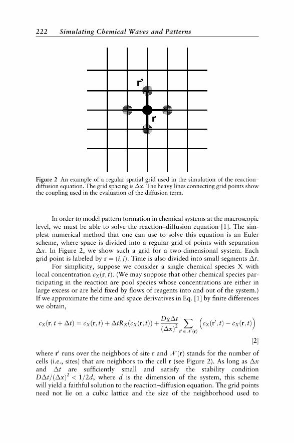
In order to model pattern formation in chemical systems at the macroscopiclevel, we must be able to solve the reaction–diffusion equation [1]. The sim-plest numerical method that one can use to solve this equation is an Eulerscheme, where space is divided into a regular grid of points with separation�x. In Figure 2, we show such a grid for a two-dimensional system. Eachgrid point is labeled by r ¼ ði; jÞ. Time is also divided into small segments �t.

For simplicity, suppose we consider a single chemical species X withlocal concentration cXðr; tÞ. (We may suppose that other chemical species par-ticipating in the reaction are pool species whose concentrations are either inlarge excess or are held fixed by flows of reagents into and out of the system.)If we approximate the time and space derivatives in Eq. [1] by finite differenceswe obtain,

cXðr; t þ�tÞ ¼ cXðr; tÞ þ�tRXðcXðr; tÞÞ þDX�t

ð�xÞ2X

r0 2NðrÞ

�cXðr0; tÞ cXðr; tÞ

�

½2�

where r0 runs over the neighbors of site r and NðrÞ stands for the number ofcells (i.e., sites) that are neighbors to the cell r (see Figure 2). As long as �xand �t are sufficiently small and satisfy the stability conditionD�t=ð�xÞ2 < 1=2d, where d is the dimension of the system, this schemewill yield a faithful solution to the reaction–diffusion equation. The grid pointsneed not lie on a cubic lattice and the size of the neighborhood used to

Figure 2 An example of a regular spatial grid used in the simulation of the reaction–diffusion equation. The grid spacing is �x. The heavy lines connecting grid points showthe coupling used in the evaluation of the diffusion term.


compute the spatial derivatives can be enlarged to insure that the chemical pat-terns do not depend on the underlying grid used in the simulations. If the reac-tion kinetics has very disparate time scales or the spatial variations of theconcentrations are very pronounced, the differential equations are called stiffand such a simple explicit scheme may not be efficient. In this case, more com-plicated implicit partial differential equation solvers or other integrationschemes may be used to obtain the solutions of the reaction–diffusion equa-tion.10–15 The simulation of two often-studied models will illustrate some ofthe chemical patterns that reaction–diffusion equations can display.

The Schlogl model16 has the reaction mechanism,

ðiÞ A Ðk1

k1

X ðiiÞ Bþ 2X Ðk2

k2

3X ½3�

We suppose that the A and B species are pool species, that is, their concentra-tions are very large. If the concentrations of these species are taken to beconstant, only the concentration of species X can change. Following massaction kinetics, the reaction rates corresponding to the two steps in themechanism (Eq. [3]) are

RðiÞX ðcXÞ ¼ k1ca k1cX

RðiiÞX ðcXÞ ¼ k2cbc2

X k2c3X

½4�

where ca and cb are the constant concentrations of species A and B, respec-tively. Consequently, the overall reaction rate for species X is RX ¼ R

ðiÞX þ

RðiiÞX ¼ k1ca k1cX þ k2cbc2

X k2c3X.

If the system is homogeneous in space, there are no concentration gradi-ents and the reaction–diffusion equation [1] reduces to the chemical rate law,

dcXðtÞdt

¼ k1ca k1cX þ k2cbc2X k2c3

X ½5�

whose steady-state concentrations c�X (i.e., those for which dcX=dt ¼ 0) aregiven by the solutions of the cubic equation, k1ca k1c�X þ k2cbc�2X k2c�3X ¼ 0. Depending on the choice of kinetic parameters, the Schloglmodel possesses either a single stable steady state or bistable steady states.A sketch of the steady-state solutions are shown in Figure 3. A rate law ofthis type is applicable to the iodate–arsenous acid system where experimentalstudies of wave propagation have been carried out.17

Suppose the initial concentration of X in the system fluctuates slightly inspace around the value c�0 so that cXðr; 0Þ ¼ c�0 þ dcXðrÞ, where dcXðrÞ is asmall perturbation. If c�0 corresponds to the unstable state and we solve the


reaction–diffusion equation for the Schlogl model in two dimensions using theEuler scheme in Eq. [2] subject to this initial condition, we obtain the resultsshown in Figure 4. The system quickly evolves from the unstable state andforms domains of the two stable states separated by chemical fronts where

Figure 3 Steady states of the Schlogl model. The steady-state concentration c�X is plottedversus the rate constant k1. The solid (dashed) lines denote stable (unstable) steadystates. Parameters are k1ca ¼ 0:001, k2cb ¼ 0:0356, and k2 ¼ 0:0153. The filled circlesare the results of a mesocopic Markov chain simulation of the Schlogl reactiondynamics.

Figure 4 Formation of domains of the two stable states in the Schlogl model color codedin gray shades.


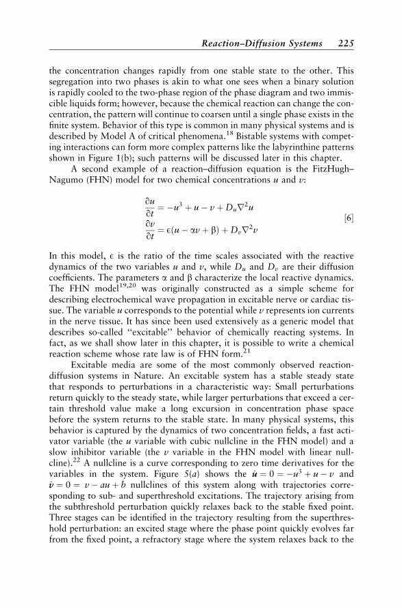
the concentration changes rapidly from one stable state to the other. Thissegregation into two phases is akin to what one sees when a binary solutionis rapidly cooled to the two-phase region of the phase diagram and two immis-cible liquids form; however, because the chemical reaction can change the con-centration, the pattern will continue to coarsen until a single phase exists in thefinite system. Behavior of this type is common in many physical systems and isdescribed by Model A of critical phenomena.18 Bistable systems with compet-ing interactions can form more complex patterns like the labyrinthine patternsshown in Figure 1(b); such patterns will be discussed later in this chapter.

A second example of a reaction–diffusion equation is the FitzHugh–Nagumo (FHN) model for two chemical concentrations u and v:

qu

qt¼ u3 þ u vþDur2u

qv

qt¼ Eðu avþ bÞ þDvr2v

½6�

In this model, E is the ratio of the time scales associated with the reactivedynamics of the two variables u and v, while Du and Dv are their diffusioncoefficients. The parameters a and b characterize the local reactive dynamics.The FHN model19,20 was originally constructed as a simple scheme fordescribing electrochemical wave propagation in excitable nerve or cardiac tis-sue. The variable u corresponds to the potential while v represents ion currentsin the nerve tissue. It has since been used extensively as a generic model thatdescribes so-called ‘‘excitable’’ behavior of chemically reacting systems. Infact, as we shall show later in this chapter, it is possible to write a chemicalreaction scheme whose rate law is of FHN form.21

Excitable media are some of the most commonly observed reaction-diffusion systems in Nature. An excitable system has a stable steady statethat responds to perturbations in a characteristic way: Small perturbationsreturn quickly to the steady state, while larger perturbations that exceed a cer-tain threshold value make a long excursion in concentration phase spacebefore the system returns to the stable state. In many physical systems, thisbehavior is captured by the dynamics of two concentration fields, a fast acti-vator variable (the u variable with cubic nullcline in the FHN model) and aslow inhibitor variable (the v variable in the FHN model with linear null-cline).22 A nullcline is a curve corresponding to zero time derivatives for thevariables in the system. Figure 5(a) shows the _uu ¼ 0 ¼ u3 þ u v and_vv ¼ 0 ¼ v auþ b nullclines of this system along with trajectories corre-sponding to sub- and superthreshold excitations. The trajectory arising fromthe subthreshold perturbation quickly relaxes back to the stable fixed point.Three stages can be identified in the trajectory resulting from the superthres-hold perturbation: an excited stage where the phase point quickly evolves farfrom the fixed point, a refractory stage where the system relaxes back to the


stable state and is not susceptible to additional perturbation, and the restingstate where the system again resides at the stable fixed point.

An excitable medium is a diffusively coupled array of such local excita-ble elements described by a reaction–diffusion equation. Imagine a local super-threshold perturbation applied to the system in the homogeneous resting state.Due to diffusive coupling, the perturbation will excite neighboring regions ofthe medium. The originally perturbed region will first relax to the refractorystate where it is no longer susceptible to perturbation, and finally back to thestable steady state. Consequently, a circular wave of excitation with a refrac-tory tail will propagate outward from the perturbation through the medium. Ifan excitable wave is broken (e.g., by an obstacle or inhomogeneity in the med-ium), since the front velocity is smaller at the tip than the rest of the wavefront, free ends of wave fronts will curl, leading to the formation of spiralwaves in the system. Examples of a ring of excitation and a spiral wave inthe FitzHugh excitable medium are shown in Figure 6.

Excitable waves are seen in many chemical and biological systems. Theoften-studied BZ reaction was one of the first systems in which such waveswere observed.4,23 Chemical waves of this type have been studied extensivelyin the catalytic oxidation of CO on Pt.24 In biological contexts, waves of thistype occur in the aggregation stage of the slime mould dictyostelium discoi-deum where the chemical signaling is through periodic waves of cyclic adeno-sine monophosphate (cAMP); also, the Ca2þ waves in systems like xenopuslaevis oocytes and pancreatic b cells fall into this category.25 Electrochemicalwaves in cardiac and nerve tissue have this origin and the appearance and/orbreakup of spiral wave patterns in excitable media are believed to be respon-sible for various types of arrhythmias in the heart.26

Figure 5 Cubic ð _uu ¼ 0Þ and linear ð _vv ¼ 0Þ nullclines for the FHN equations: (a) displaysthe excitable dynamics showing trajectories resulting from sub- and super-thresholdexcitations; (b) displays oscillatory dynamics showing two limit cycle orbits; small innerlimit cycle close to Hopf point; large outer limit cycle far from Hopf point. See Ref. 7 forthe definition of Hopf points.


In addition to excitability, the FHN model can also possess oscillatorysolutions. Figure 5(a) shows the configuration of the nullclines for a differentchoice of parameters. Now the system has an unstable fixed point or steadystate and the stable attracting state is a limit cycle oscillation shown as theclosed loop surrounding the unstable fixed point in the ðuvÞ-plane of the figure.Chemical patterns such as spiral waves can form in oscillatory as well as exci-table systems27 and we shall have occasion to discuss some aspects of patternsin oscillatory media below.

CELLULAR AUTOMATA

The chemically reacting systems we have been considering are relativelysimple—at least our models for them have been so. However, most of thepattern forming reacting media studied in the laboratory have very complexmechanisms whose full nature is still a matter of debate, even for the exten-sively studied BZ reaction.28 The situation becomes very complicated indeedif one turns to living systems where the basic underlying mechanisms involvevery complex networks of reactions. One question one might pose is, are therecertain basic underlying principles or mechanisms that complex systemsexploit to achieve a particular kind of behavior? Or, stated another way,are there simple rules that underlie the dynamics of complex systems?

Cellular automata were constructed by Von Neumann and Ulam as sim-ple models of self-reproducing systems that mimic living systems.29 The VonNeumann cellular automaton is not so simple and comprises a fairly complexset of rules that specifies how the system evolves in time. Codd devised a muchsimpler rule that achieves self-reproduction.30,31 Wiener and Rosenbluth

Figure 6 A ring of excitation (a) and a spiral wave (b) calculated from the excitable FHNmedium, Eq. [6].

Cellular Automata 227

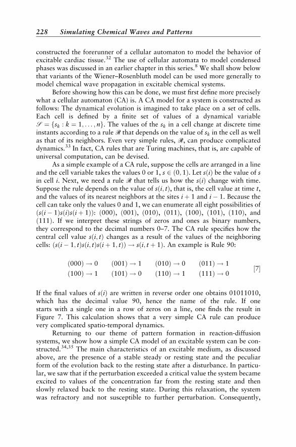
constructed the forerunner of a cellular automaton to model the behavior ofexcitable cardiac tissue.32 The use of cellular automata to model condensedphases was discussed in an earlier chapter in this series.8 We shall show belowthat variants of the Wiener–Rosenbluth model can be used more generally tomodel chemical wave propagation in excitable chemical systems.

Before showing how this can be done, we must first define more preciselywhat a cellular automaton (CA) is. A CA model for a system is constructed asfollows: The dynamical evolution is imagined to take place on a set of cells.Each cell is defined by a finite set of values of a dynamical variableS ¼ fsk : k ¼ 1; . . . ; ng. The values of the sk in a cell change at discrete timeinstants according to a rule R that depends on the value of sk in the cell as wellas that of its neighbors. Even very simple rules, R, can produce complicateddynamics.33 In fact, CA rules that are Turing machines, that is, are capable ofuniversal computation, can be devised.

As a simple example of a CA rule, suppose the cells are arranged in a lineand the cell variable takes the values 0 or 1, s 2 ð0; 1Þ. Let sðiÞ be the value of sin cell i. Next, we need a rule R that tells us how the sðiÞ change with time.Suppose the rule depends on the value of sði; tÞ, that is, the cell value at time t,and the values of its nearest neighbors at the sites iþ 1 and i 1. Because thecell can take only the values 0 and 1, we can enumerate all eight possibilities ofðsði 1ÞsðiÞsðiþ 1ÞÞ: ð000Þ, ð001Þ, ð010Þ, ð011Þ, ð100Þ, ð101Þ, ð110Þ, andð111Þ. If we interpret these strings of zeros and ones as binary numbers,they correspond to the decimal numbers 0–7. The CA rule specifies how thecentral cell value sði; tÞ changes as a result of the values of the neighboringcells: ðsði 1; tÞsði; tÞsðiþ 1; tÞÞ ! sði; t þ 1Þ. An example is Rule 90:

ð000Þ ! 0 ð001Þ ! 1 ð010Þ ! 0 ð011Þ ! 1

ð100Þ ! 1 ð101Þ ! 0 ð110Þ ! 1 ð111Þ ! 0½7�

If the final values of sðiÞ are written in reverse order one obtains 01011010,which has the decimal value 90, hence the name of the rule. If onestarts with a single one in a row of zeros on a line, one finds the result inFigure 7. This calculation shows that a very simple CA rule can producevery complicated spatio-temporal dynamics.

Returning to our theme of pattern formation in reaction-diffusionsystems, we show how a simple CA model of an excitable system can be con-structed.34,35 The main characteristics of an excitable medium, as discussedabove, are the presence of a stable steady or resting state and the peculiarform of the evolution back to the resting state after a disturbance. In particu-lar, we saw that if the perturbation exceeded a critical value the system becameexcited to values of the concentration far from the resting state and thenslowly relaxed back to the resting state. During this relaxation, the systemwas refractory and not susceptible to further perturbation. Consequently,


we can identify three major states of the system: the resting state Q, the excitedstate E, and the refractory state R. To construct a CA model for an excitablesystem, we suppose that the cells in the CA model can take values in the setS ¼ fQ;E;Rg. We arrange the cells on a regular lattice in space, say in twodimensions, as shown in Figure 2 for the discretization of the reaction–diffu-sion equation. Now all we need is a rule R that changes the state of the cellsand mimics the excitable dynamics.

First, consider a cell in isolation from its neighboring cells. If it is in theresting state Q, it will remain there since this is the stable steady state of thesystem. If it is excited, that is, in the state E, it will first become refractory, andthen finally return to the resting state. Thus, it will undergo the series ofchanges E! R! Q.

Of course, cells are not isolated but communicate with their neighborsmimicking the diffusion of chemicals in the real system. We can take thiscoupling effect into account by having the state of a cell labeled by r, itsdiscrete position on the lattice, change as a result of the values in neighboringcells located at sites r0. In particular, we suppose that if the cell at r is in itsresting state Q and any one of the neighboring cells is excited; that is, inthe state E, then in the next step the cell will become excited. If we letsðr; tÞ be the state of the cell r at time t, then the rule R for an excitablemedium may be written compactly as

sðr; t þ 1Þ ¼E if sðr; tÞ ¼ Q and sðr0; tÞ ¼ ER if sðr; tÞ ¼ EQ if sðr; tÞ ¼ R or sðr; tÞ ¼ Q and sðr0; tÞ 2 fQ;Rg

8<: ½8�

By using this rule, it is possible to construct the evolution of simple initialconditions with just a pencil and graph paper. For example, if all the cells in

Figure 7 Time evolution given by Rule 90. The abcissa is the cell label while the ordinateis discrete time, with time increasing from top to bottom. The color coding is such that 0is white and 1 is black.


the system are in the resting Q state except for a single cell in the center that isexcited and in state E, then, according to the rule this central cell will excite itsneighbors to the state E, while it will evolve to the refractory state R. In sub-sequent time steps, the excited cells will continue to excite neighboring cellsthat are in the resting state Q, but will not excite cells in the refractory stateR, since this state is not susceptible to perturbations. Thus a ring of excitationwill grow from the single excited cell as shown in Figure 8. The analogy withthe growing ring of excitation in the partial differential equation (PDE) simu-lation of the FHN model in Figure 6 is evident.

Spiral waves are also easily generated by this CA rule. To produce suchchemical waves in the system, we start with an initial condition consisting of arow of cells in the excited state E, adjacent to a row of cells in the refractorystate R. All other cells in the system are in the resting state Q. The cells in thecenter of the row simply advance forward on each time step as the excited cellsexcite their neighbors; backward excitation is prevented by the row of refrac-tory cells. However, more interesting behavior occurs at the end of the row.Because an additional cell may be excited at the end of the row in thefirst time step, the excitation will ‘‘curl’’ around the refractory states at subse-quent time steps leading to a pair of spiral waves as shown in Figure 9. Onceagain the similarity to the spiral wave in Figure 6 for the FHN model isevident.

Figure 8 A ring of excitation produced by the excitable medium CA rule. Color coding:Q white, E black, R shaded.

Figure 9 A spiral wave produced by the excitable medium CA rule.


This example illustrates both the power and drawbacks of simple cellularautomaton modeling of reaction–diffusion media. The CA rule abstracts theessential features responsible for the different types of wave propagationseen in excitable media and provides considerable insight into how and whysuch chemical patterns form. However, if one wants to examine the chemicalpatterns in excitable media in more detail, the artifacts arising from the sim-plicity of the CA rule are an obstacle to such investigations. For example, oneobvious difference between the ring of excitation and spiral patterns in the CAmodel and those in the PDE simulation of the FHN model is that the CA pat-terns have sharp corners. The shapes of the waves are also determined by thenature of the lattice on which the CA cells are placed and the nature ofthe neighborhood used in the CA rule. For example, if nearest plus next-near-est neighbors (called a Moore neighborhood) are used to update the cellvalues, one obtains a square-shaped ring instead of a diamond-shaped ring.Since the curvature of the wave fronts determines many aspects of theirpropagation properties, a quantitative description of wave propagation isnot possible using this CA model.

It is also interesting to examine the nature of the center or core of thespiral wave in the CA model. By looking at the evolution of the CA spiralwave in Figure 9 one can see that there is a configuration of four cells (shownin Figure 10) that cycles and repeats itself every four time steps. This cyclingconfiguration is responsible for the generation of the spiral wave and does notmove: The spiral is pinned to the initial location of this core configuration ofcells. In experimental observations of spiral waves of excitable chemical mediaand PDE simulations, depending on the system parameters, the spiral core isnot stationary and may undergo complicated meandering motion.36–39 Thisbehavior is not captured by the simple CA model.

One can now envisage several ways to try to remedy these deficienciesand there have been numerous generalizations of the simple excitable CArule discussed above.40,41 These generalizations typically increase the size ofthe state space of a cell, including several excited and refractory states.

Figure 10 Cycling configuration of cells at the center or core of a CA spiral wave.


Furthermore, the size and nature of the neighborhood can be changed. If theCA rules are made sufficiently elaborate many of the artifacts of the waves canbe removed. However, the price one pays is the lack of simplicity and physicalinsight and increased computational cost. Direct simulation of PDE models isa simple task on current computers, precluding the use of such elaborate CAmodels.

However, in addition to the physical insight into the nature of excitablewave propagation that CA models provide, they are a powerful tool for ana-lyzing general aspects of complex dynamics. Thus, their utility far surpassesthe fact that they are simple models for reaction–diffusion systems. Becausevery simple rules can yield very complicated dynamical behavior, these modelshave been investigated extensively in the mathematical and physical litera-ture.42,43 They provide insight into the basic conditions needed to obtain com-plex behavior and provide a means of classifying this behavior. The fact thatsimple CA rules can lead to universal computation or self-replication provideskeys to a deeper understanding of Nature.

COUPLED MAP LATTICES

In the preceding two sections, we discussed patterns in chemically reactingmedia using PDE reaction–diffusion models, where space, time, and chemicalconcentrations were continuous variables, and cellular automata, where space,time, and the state of a cell were discrete. We now turn our attention tocoupled map lattices (CML),44,45 another type of model that has been usedto gain insight into the behavior of systems displaced far from equilibrium.The structure of a CML model of a system has similarities both to discretiza-tions of reaction–diffusion equations and to cellular automata. To build aCML model of a system, space is partitioned into a grid of points on whichthe dynamical variables (chemical concentrations in our case) are evaluated.A rule or map is associated with each lattice site that specifies how the vari-ables change after a single time step. The rule differs from that used in a CAmodel since the variables in the cells can take continuous values, not discretevalues as in a CA rule, and the map function specifies how these continuousvariables change in one time step. The coupled map lattice is constructed bycoupling such maps together so that the new value of the variable at the site isdetermined by the local map plus its coupling to the maps at neighboring sites.Thus, we see that in a CML both space and time are discrete while the dyna-mical variable at a site takes on continuous values.

We may again use the grid in Figure 2 to show how the maps maybe coupled to form CML. As in our earlier discussions the sites of thelattice are labeled by discrete values r. At each site we have a map that is afunction f ðcðr; tÞÞ that takes the variable cðr; tÞ at site r at time t into its


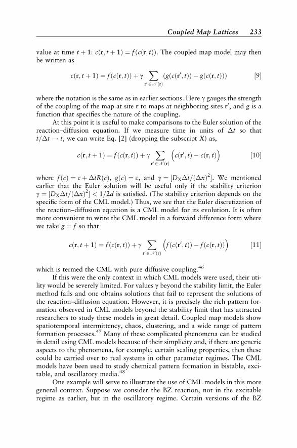
value at time t þ 1: cðr; t þ 1Þ ¼ f ðcðr; tÞÞ. The coupled map model may thenbe written as

cðr; t þ 1Þ ¼ f ðcðr; tÞÞ þ gX

r0 2NðrÞðgðcðr0; tÞÞ gðcðr; tÞÞÞ ½9�

where the notation is the same as in earlier sections. Here g gauges the strengthof the coupling of the map at site r to maps at neighboring sites r0, and g is afunction that specifies the nature of the coupling.

At this point it is useful to make comparisons to the Euler solution of thereaction–diffusion equation. If we measure time in units of �t so thatt=�t! t, we can write Eq. [2] (dropping the subscript X) as,


r0 2NðrÞ

�cðr0; tÞ cðr; tÞ

�½10�

where f ðcÞ ¼ cþ�tRðcÞ, gðcÞ ¼ c, and g ¼ ½DX�t=ð�xÞ2�. We mentionedearlier that the Euler solution will be useful only if the stability criteriong ¼ ½DX�t=ð�xÞ2� < 1=2d is satisfied. (The stability criterion depends on thespecific form of the CML model.) Thus, we see that the Euler discretization ofthe reaction–diffusion equation is a CML model for its evolution. It is oftenmore convenient to write the CML model in a forward difference form wherewe take g ¼ f so that


r0 2NðrÞ

�f ðcðr0; tÞÞ f ðcðr; tÞÞ

�½11�

which is termed the CML with pure diffusive coupling.46

If this were the only context in which CML models were used, their uti-lity would be severely limited. For values g beyond the stability limit, the Eulermethod fails and one obtains solutions that fail to represent the solutions ofthe reaction–diffusion equation. However, it is precisely the rich pattern for-mation observed in CML models beyond the stability limit that has attractedresearchers to study these models in great detail. Coupled map models showspatiotemporal intermittency, chaos, clustering, and a wide range of patternformation processes.47 Many of these complicated phenomena can be studiedin detail using CML models because of their simplicity and, if there are genericaspects to the phenomena, for example, certain scaling properties, then thesecould be carried over to real systems in other parameter regimes. The CMLmodels have been used to study chemical pattern formation in bistable, exci-table, and oscillatory media.48

One example will serve to illustrate the use of CML models in this moregeneral context. Suppose we consider the BZ reaction, not in the excitableregime as earlier, but in the oscillatory regime. Certain versions of the BZ

Coupled Map Lattices 233

reaction are light sensitive. If the BZ reaction is carried out in a CFUR andsubjected to periodic illumination, the external periodic forcing of the oscilla-tory medium can give rise to a new class of chemical patterns.49,50 If the periodof the forcing by the illumination is close to a multiple of the natural periodof the oscillation, the system can become locked or entrained to some multipleof the driving period. An example of the experimental results for such a per-iodically forced oscillatory reaction–diffusion system is shown in Figure 11.The figure shows that the system can lock to different multiples of the drivingfrequency of the light (labeled 1:1, 1:2, 1:3, etc., in the figure) and that thesystem forms patches where the chemical concentrations are similar, separatedby fronts where the phase of the oscillation jumps by some multiple of p. Forexample, in the right-most panel we have 3:1 mode locking. Here we see threedifferent types of patches coded by white, gray, and black. If we observe onepatch, at time intervals corresponding to the external forcing period, it willcycle according to white! black! gray! white. If we compare the upperand lower panels of the figure, we can see such a change of colors of the homo-geneous patches. We can associate a phase n2p=3, n ¼ 1; 2; . . . with each col-or. Thus, we see that the periodic forcing has turned the continuous oscillationinto an oscillation with discrete phases in this representation: The periodicforcing has broken the time translation symmetry of the system.

What has all of this to do with coupled map lattices? Suppose we take aCML model where the local map at a site leads to cycling among three states: aperiod-3 map. An example is

f ðzÞ ¼ bz for 0 � z � 1=ba for 1=b < z � 1

�½12�

Figure 11 Resonantly forced patterns in the oscillatory light-sensitive BZ medium (fromRef. 49).


The map f ðzÞ possesses the period-3 solution A ¼ a! B ¼ ab! C ¼ ab2 !A ¼ a (see Figure 12 for a graphical representation). The local map hasthe same discrete period-3 behavior as the local dynamics of the resonantlyforced system. The discrete time dynamics of the map breaks the time transla-tion symmetry of the system just like the resonant forcing of the local chemicaldynamics. We can now make a CML model of the resonantly forced 3:1reaction–diffusion system by coupling an array of such period-3 maps:

zðr; t þ 1Þ ¼ f ðzðr; tÞÞ þ gX

r0 2NðrÞ

�f ðzðr0; tÞÞ f ðzðr; tÞ

�½13�

with the notation as used earlier. The CML model is simple to simulate ona computer. If we start with three patches of the three different values ofthe period-3 orbit, we obtain the result shown in Figure 13. This figure shouldbe compared with the last panel of Figure 11, where similar coexistencebetween periodic homogeneous phases, is seen. As in the resonantly forcedchemical systems, the colors of the homogeneous patches in the pattern shownin Figure 13 cycle among themselves.

This CML model does not attempt to account for the detailed features ofthe chemistry of the resonantly forced BZ reaction; instead, like CA models, itfocuses on the generic element needed to observe the pattern (in this case thebroken time translation symmetry produced by the external forcing). TheCML model may then be used to explore the possible types of patterns thatmay arise in systems with this characteristic feature. In this way, we cangain insight into how such patterns form and even discover new types of pos-sible behavior.

Figure 12 The piece-wise linear map for parameters that support a stable period-3 orbit.The period-3 orbit is shown graphically.

Coupled Map Lattices 235

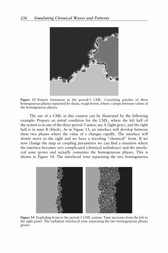
The use of a CML in this context can be illustrated by the followingexample: Prepare an initial condition for the CML, where the left half ofthe system is in one of the three period-3 states, say A (light gray), and the righthalf is in state B (black). As in Figure 13, an interface will develop betweenthese two phases where the value of z changes rapidly. The interface willslowly move to the right and we have a traveling ‘‘chemical’’ front. If wenow change the map or coupling parameters we can find a situation wherethe interface becomes very complicated (chemical turbulence) and the interfa-cial zone grows and actually consumes the homogeneous phases. This isshown in Figure 14. The interfacial zone separating the two homogeneous

Figure 13 Pattern formation in the period-3 CML. Coexisting patches of threehomogeneous phases separated by sharp, rough fronts, where z jumps between values ofthe homogeneous phases.

Figure 14 Exploding front in the period-3 CML system. Time increases from the left tothe right panel. The turbulent interfacial zone separating the two homogeneous phasesgrows.


phases grows with time and if the simulation were continued the chaoticphase would fill the entire system resulting in a complicated state termedspatio-temporal turbulence. For other parameter values, the turbulent zoneis confined between the two stable phases. Thus, the system exhibits a typeof nonequilibrium phase transition between a complex, but confined, interfa-cial zone and a turbulent phase that consumes the homogeneous phases.51,52

Is this behavior a peculiar feature of the CML model or is it real?Figure 15 shows the results of a simulation of a 3:1 resonantly forced oscilla-tory reaction–diffusion system for a specific choice of parameters.53,54 As inthe CML model, a chemical front separates two of the three homogeneousphases. This front is turbulent and grows to fill the entire system. This suggeststhat the phenomenon is real and may be found in resonantly forced chemicalsystems.

MESOSCOPIC MODELS

The models for chemically reacting media discussed above described theevolution of the system on macroscopic scales. In some instances, especiallywhen one considers applications of nonlinear chemical dynamics to biologicalsystems or materials on nanoscales, a mesoscopic description will be moreappropriate or even essential. In this section, we show how one can constructmesoscopic models for reaction–diffusion systems and how these more funda-mental descriptions relate to the macroscopic models considered previously.

In order to construct mesoscopic models, we again begin by partitioningthe system into cells located at the nodes of a regular lattice, but now the cellsare assumed to contain some small number of molecules. We cannot use a con-tinuum description of the dynamics in a cell as we did for the reaction–diffu-sion equation. Instead, we describe the reactions and motions of moleculesusing stochastic rules that mimic the dynamics of these processes on meso-scales. The stochastic element arises because we do not take into accountthe detailed motions of all solvent species or the dynamics on microscopicscales. Nevertheless, because the number of molecules in a cell may be small,we must account for the fact that this number can change by random reactiveevents and random motions of molecules that take them into and out of a

Figure 15 Exploding front in a 3:1 resonantly forced oscillatory reaction–diffusionsystem. Time increases from panel a to panel b.

Mesoscopic Models 237

given cell. A schematic picture of the cell structure for a mesoscopic model isshown in Figure 16. The nodes or cells of the regular lattice with N sites arelabeled by rN ¼ ðr1; r2; . . . ; rNÞ. A site ri has nXðriÞ molecules of species X.We are interested in the probability PðnN

X ; tÞ that the set of N nodes havenN

X ¼ ðnXðr1Þ; nXðr2Þ; . . . ; nXðrNÞÞ molecules of species X at time t.The equation that governs the time evolution of this probability distribu-

tion is taken to be the Markov process model,55,56

qPðnNX ; tÞ

qt¼Xn0NX

W nNX jn0

NX

� �P n0

NX ; t

� �½14�

where the transition probability matrix W specifies how PðnXN; tÞ changes

because of diffusion of particles from cell to cell and reactions within the cells.Alternatively, we can model the dynamics by Markov chain models57

PðnNX ; t þ 1Þ ¼

Xn0NX

~WW nNX jn0

NX

� �P n0

NX ; t

� �½15�

where the time is discrete as in CA or CML models.Random-walk models for diffusion on the lattice can be implemented in

various ways. Typically, particles randomly hop between a node r andits neighbors r0 2NðrÞ. If there are no restrictions on the number of particlesat a node, the stationary distribution for this diffusive stochastic process isPoissonian,55

PðnX; cXÞ ¼cnX

X

nX!ecX ½16�

Figure 16 Cell structure used in the construction of mesoscopic models. The number ofparticles in the cells can change by stochastic reaction rules and by random motion intoand out of the cell volumes (shown schematically by arrows).


where cX is the average density of species X on the lattice. Diffusion may alsobe modeled by a random walk with exclusion. This may be accomplished inmany ways. (For a review of reactive lattice-gas automata, see Ref. 58). Sup-pose a maximum number of m particles of species X is allowed at a node; then,for example, particles may be assigned to channels corresponding to the linksof the lattice. The channel configuration may be randomized and particles pro-pagated synchronously and deterministically to neighboring lattice nodes. Thisleads to a binomial distribution

PðnX; cXÞ ¼mnX

� cX

m

� �nX

1 cX

m

� �mnX

½17�

if small correlations arising from exclusion are neglected.As a simple illustration of how reactions may be treated stochastically on

mesoscopic scales, we show how one may construct a mesoscopic Markovprocess model for the Schlogl reaction (Eq. [3]). As before, we assume that spe-cies A and B in the Schlogl mechanism are pool species and their concentra-tions do not change in time: Their effect is incorporated into the rateconstants of the reaction. A Markov model of the reactions is a birth–deathprocess, where chemical species are ‘‘born’’ in some reactions (X is born inthe reactions (1) A! X and (3) 2Xþ B! 3X) and ‘‘dies’’ in others (X diesin the reactions (2) X! A and (4) 3X! 2Xþ B). Suppose there are nX mole-cules of species X in a cell. Then the probability that a reaction X! A occursand changes the number of molecules in the cell from nX to n0X ¼ nX 1 is just

X!k1A p2ðnXjnX 1Þ ¼ k1nX ½18�

Similarly, for the other reactions, we have

A!k1X p1ðnXjnX þ 1Þ ¼ k1nA ½19�

2Xþ B!k23X p3ðnXjnX þ 1Þ ¼ k2nXðnX 1ÞnB ½20�

3X!k22Xþ B p4ðnXjnX 1Þ ¼ k2nXðnX 1ÞðnX 2Þ ½21�

Given these reaction probabilities, we can write the rate of change of the prob-ability that there are nX molecules of species X in the cell at time t, PðnX; tÞ, as

dPðnX; tÞdt

¼�

k1nA þ k2ðnX 1ÞðnX 2ÞnB

�PðnX 1; tÞ

þ�

k1ðnX þ 1Þ þ k2ðnX þ 1ÞnXðnX 1Þ�

PðnX þ 1; tÞ

�

k1nA þ k1nX þ k2nXðnX 1ÞnB

þ k2nXðnX 1ÞðnX 2Þ�

PðnX; tÞ ½22�


The average concentration of species X at time t is given by cXðtÞ ¼PnX

nXPðnX; tÞ. If diffusion is sufficiently rapid to maintain the system in localequilibrium so that the distribution of molecules in the cells is Poissonian,characterized by the instantaneous value of the chemical concentration, wemay replace PðnX; tÞ in Eq. [22] by Pðnx; cxðtÞÞ and compute the time rate ofchange of the average value of the concentration of species X as

dcXðtÞdt

¼X1nX¼0

nX

h�k1nA þ k2ðnX 1ÞðnX 2ÞnB

�PðnX 1; cXðtÞÞ

þ�

k1ðnX þ 1Þ þ k2ðnX þ 1ÞnXðnX 1Þ�

PðnX þ 1; cXðtÞÞ

�

k1nA þ k1nX þ k2nXðnX 1ÞnB þ k2nXðnX 1ÞðnX 2Þ�i

� PðnX; cXðtÞÞ ¼ k1a k1cX þ k2bc2X k2c3

X ½23�

Thus, we find the macroscopic chemical rate law for the Schlogl model.Mesoscopic simulations of the Schlogl model have been carried out using aMarkov chain model.59 Figure 3 shows the results for the steady-state concen-trations derived from such a mesoscopic simulation along with the determinis-tic steady-state concentrations discussed earlier. The stochastic model yieldsresults that are close to those of the mass action rate law. However, in thevicinities of points where the deterministic stable and unstable fixed pointsmeet, so that one of the stable states loses its stability, fluctuations play animportant role.

Stochastic models are also able to capture complicated pattern formationseen in chemically reacting media and can be used to study the effects of fluc-tuations on chemical patterns and wave propagation. The mesoscopicdynamics of the FHN model illustrates this point. In order to formulate amicroscopically based stochastic model for this system, it is first necessaryto provide a mechanism whose mass action law is the FHN kinetic equation.Some features of the FHN kinetics seem to preclude such a mechanisticdescription; for example, the production of u is inhibited by a term linear inv, a contribution not usually encountered in mass action kinetics. However,if each local region of space is assumed to be able to accommodate only amaximum number m of each chemical species, then such a mechanism maybe written.21 We assume that the chemical reactions depend on the localnumber of molecules of the species as well as the number of vacancies corre-sponding to each species, in analogy with the dependence of some surface reac-tions on the number of vacant surface sites or biochemical reactions involvingcomplexes of allosteric enzymes that depend on the number of vacant activesites.


The reaction mechanism consists of the cubic autocatalytic steps involv-ing species A and its corresponding vacancy species A�,

2Aþ A� !k13A

2A� þ A!k�

13A�

½24�

This part of the mechanism is responsible for the bistability of the system but,in the absence of other coupling, will simply give rise to stable states corre-sponding to full occupancy or complete vacancy at a site. A second speciesB involved in bimolecular reactions with A is needed to account for boththe linear and cubic parts of the FHN model. The cyclic reaction steps,

A� þ B!k2Aþ B

k�3 " # k3

A� þ B� k�

2Aþ B�

½25�

produce this effect. Assuming mass action kinetics, we may write the chemicalrate law that follows from this mechanism as

dca

dt¼ fk1ca k�1ð1 caÞgcað1 caÞ þ k2ð1 caÞcb k�2cað1 cbÞ

dcb

dt¼ k�3ð1 caÞð1 cbÞ k3cacb

½26�

where ca and cb are the average concentrations of A and B at a site (fractionaloccupancies). While this rate law does not seem to correspond to FHNkinetics, for k�2 ¼ k2 and k�3 ¼ k3, these equations can be converted to FHNform by making the linear change of variables, ca ¼ auþ a0 andcb ¼ bvþ b0 where

a2 ¼ 1

3

k1 þ 2k�1k1 þ k�1

� 2

k2 þ k�1k1 þ k�1

a0 ¼1

3

k1 þ 2k�1k1 þ k�1

b ¼ k1 þ k�1k2

c3a b0 ¼ a0

cb

ca1 a0

ca

� 2( ) ½27�

and use of the scaled time variable t ¼ t=ts with t1s ¼ ðk1 þ k�1Þa2. The para-

meters in Eq. [6] are related to the rate constants by

a ¼ cb

cab ¼ 1 a0 b0

caE ¼ k3

k2

ca

cb

� 2

½28�


Once a mechanism for a reaction is given, we may use the birth–deathkinetic rules to write a stochastic mesoscopic model for the reaction and diffu-sion processes. Figure 17 presents the results of a simulation of the FHNmechanism using a Markov chain model that shows the formation of achemical labyrinthine pattern in a region where the FHN model has two stablesteady states.21 This complicated pattern arises from the nonlinear kinetics inthe FHN mechanism and the long-range coupling between spatial points in thesystem because of rapid diffusion of species B relative to that of species A. Thiscauses two chemical fronts to repel each other when they are sufficiently close.Consequently, the domains of the two stable phases in the labyrinthine patternseen in the last panel of this figure will not ‘‘coarsen’’ like the domains of thetwo stable phases of the Schlogl model shown in Figure 4. Labyrinthinepatterns of this type have been observed experimentally in reaction–diffusionsystems with two stable steady states (see Figure 1b).60 Stochastic models ofthis kind can be used to investigate the influence of fluctuations on patterns,especially on patterns that exist on small nanoscales as a result of competinginteractions.61

Figure 17 Formation of a labyrinthine pattern in a Markov chain model of the FHNsystem.


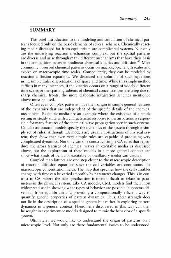
SUMMARY

This brief introduction to the modeling and simulation of chemical pat-terns focused only on the basic elements of several schemes. Chemically react-ing media displaced far from equilibrium are complicated systems. Not onlyare the underlying reaction mechanisms complex, but the spatial patternsare diverse and arise through many different mechanisms that have their basisin the competition between nonlinear chemical kinetics and diffusion.62 Mostcommonly observed chemical patterns occur on macroscopic length scales andevolve on macroscopic time scales. Consequently, they can be modeled byreaction–diffusion equations. We discussed the solution of such equationsusing simple Euler discretizations of space and time. While this simple methodsuffices in many instances, if the kinetics occurs on a range of widely differenttime scales or the spatial gradients of chemical concentrations are steep due tosharp chemical fronts, the more elaborate integration schemes mentionedabove must be used.

Often even complex patterns have their origin in simple general featuresof the dynamics that are independent of the specific details of the chemicalmechanism. Excitable media are an example where the existence of a stableresting or steady state with a characteristic response to perturbations is respon-sible for many features of the chemical wave propagation seen in such systems.Cellular automaton models specify the dynamics of the system through a sim-ple set of rules. Although CA models are usually abstractions of any real sys-tem, they show that even very simple rules are capable of producing verycomplicated dynamics. Not only can one construct simple CA rules that repro-duce the gross features of chemical waves in excitable media as discussedabove, but the exploration of these models in a more general context canshow what kinds of behavior excitable or oscillatory media can display.

Coupled map lattices are one step closer to the macroscopic descriptionof reaction–diffusion equations since the cell variables are continuous likemacroscopic concentration fields. The map that specifies how the cell variableschange with time can be varied smoothly by parameter changes. This is in con-trast to CA, where the rule specification is often difficult to relate to para-meters in the physical system. Like CA models, CML models find their mostwidespread use in showing what types of behavior are possible in systems dri-ven far from equilibrium and providing a computationally efficient way toquantify generic properties of pattern dynamics. Thus, their strength doesnot lie in the description of a specific system but rather in exploring patterndynamics in a general context. Phenomena discovered in this way can thenbe sought in experiment or models designed to mimic the behavior of a specificsystem.

Ultimately, we would like to understand the origin of patterns on amicroscopic level. Not only are there fundamental issues to be understood,

Summary 243

but the physical situation itself may demand such a more detailed level ofdescription. The mesoscopic models discussed in the last part of this chapterprovide one route to describe the system on more microscopic scales. Whilethese models do not provide a full microscopic description of the dynamics(this is the role of molecular dynamics simulation methods), they do incorpo-rate molecular fluctuations that are absent in the macroscopic models. Funda-mental questions, such as the validity of macroscopic rate laws for systemswith deterministic chaos, can be explored by using such models.63,64 Thedescription of the biochemistry inside the cell likely demands such mesoscopicmodels since the chemistry is complex, cell volumes are small, and the numberof chemical species in important reactions is too small to validate a descriptionin terms of mass action kinetics.65 Such approaches will likely see significantdevelopment in the future as our ability to probe chemical dynamics on smallscales increases.

REFERENCES

1. W. Y. Tam, W. Horsthemke, Z. Noszticzius, and H. L. Swinney, J. Chem. Phys., 88, 3395(1988). Sustained Spiral Waves in a Continuously Fed Unstirred Chemical Reactor.

2. B. P. Belousov, in Sbornik Referatov po Radiatsionni Meditsine Moscow, Medgiz, Moscow,1958. A Periodic Reaction and Its Mechanism.

3. A. M. Zhabotinsky, Biofizika, 9, 306 (1964). Periodic Processes of the Oxidation of MalonicAcid in Solution.

4. A. N. Zaikin and A. M. Zhabotinsky, Nature (London), 225, 535 (1970). ConcentrationWave Propagation in Two-Dimensional Liquid-Phase Self-Oscillating System.

5. A. L. Belmonte, O. Y. Qi, and J.-M. Flesselles, J. Phys. II France, 7, 1425 (1997). ExperimentalSurvey of Spiral Dynamics in the Belousov Zhabotinsky Reaction.

6. K. J. Lee and H. L. Swinney, Phys. Rev. E, 51, 1899 (1995). Pattern Formation by InteractingChemical Fronts.

7. R. Larter and K. Showalter, in Reviews in Computational Chemistry, K. B. Lipkowitz andD. B. Boyd, Eds., VCH Publishers, New York, 1997, Vol. 10, pp. 177–270. ComputationalStudies in Nonlinear Dynamics.

8. L. B. Kier, C.-K. Chang, and P. G. Seybold, in Reviews in Computational Chemistry, K. B.Lipkowitz and D. B. Boyd, Eds., Wiley-VCH, New York, 1997, Vol. 17, pp. 205–254.Cellular Automata Models of Aqueous Solution Systems.

9. R. Kapral, J. Math. Chem., 6, 113 (1991). Discrete Models for Chemically Reacting Systems.

10. G. Rousseau and R. Kapral, Chaos, 10, 812 (2000). Asynchronous Algorithm for Integrationof Reaction–Diffusion Equations for Inhomogeneous Excitable Media.

11. D. Barkley, Physica D, 49, 61 (1991). A Model for Fast Computer Simulation of Spiral Wavesin Excitable Media.

12. E. M. Cherry, H. S. Greenside, and C. S. Henriquez, Phys. Rev. Lett., 84, 1343 (2000). ASpace–Time Adaptive Method for Simulating Complex Cardiac Dynamics.

13. F. Fenton and A. Karma, Chaos, 8, 20 (1998). Vortex Dynamics in Three-DimensionalContinuous Myocardium with Fiber Rotation: Filament Instability and Fribrillation.

14. M. Dowle, R. M. Mantel, and D. Barkley, Int. J. Bifurcat. Chaos, 7, 2529 (1997). FastSimulations of Waves in Three-Dimensional Excitable Media.


15. W. L. Quan, S. J. Evans and H. M. Hastings, IEEE Trans. Biomed. Eng., 45, 372 (1998).Efficient Integration of a Realistic Two-Dimensional Cardiac Tissue Model by DomainDecomposition.

16. F. Schlogl, Z. Phys., 253, 147 (1972). Chemical Reaction Models for Nonequilibrium PhaseTransitions.

17. A. Hanna, A. Saul, and K. Showalter, J. Am. Chem. Soc., 104, 3838 (1982). Detailed Studiesof Propagating Fronts in the Iodate Oxidation of Arsenous Acid.

18. P. C. Hohenberg and B. I. Halperin, Rev. Mod. Phys., 49, 435 (1977). Theory of DynamicalCritical Phenomena.

19. R. FitzHugh, Biophys. J., 1, 445 (1961). Impulses and Physiological States in TheoreticalModels of Nerve Membrane.

20. J. S. Nagumo, S. Arimoto, and Y. Yoshikawa, Proc. IRE, 50, 2061 (1962). Active PulseTransmission Line Simulating Nerve Axon.

21. A. Malevanets and R. Kapral, Phys. Rev. E, 55, 5657 (1997). Microscopic Model forFitzHugh-Nagumo Dynamics.

22. P. Fife, in Non-Equilibrium Dynamics in Chemical Systems, C. Vidal and A. Pacault, Eds.,Springer-Verlag, Berlin, 1984, pp. 76–88. Propagator-Controller Systems and ChemicalPatterns.

23. A. T. Winfree, Science, 175, 634 (1972). Spiral Waves of Chemical Activity.

24. G. Ertl, Adv. Catal., 37, 213 (1990). Oscillatory Catalytic Reactions at Single CrystalSurfaces.

25. A. Goldbeter, Biochemical Oscillations and Cellular Rhythms, Cambridge University Press,Cambridge, 1996.

26. A. T. Winfree, When Time Breaks Down: Three Dimensional Dynamics of ElectrochemicalWaves and Cardiac Arrythmias, Princeton University Press, Princeton, 1987.

27. Y. Kuramoto, Chemical Oscillations, Waves and Turbulence, Springer-Verlag, Berlin,1980.

28. R. J. Field and M. Burger, Eds., Oscillations and Travelling Waves in Chemical Systems,Wiley, New York, 1985.

29. J. Von Neumann, in Theory of Self-Reproducing Automata, A. W. Burks, Ed., University ofIllinois, Urbana, IL, 1966.

30. E. F. Codd, Cellular Automata, Academic Press, New York, 1986.

31. C. G. Langton, Physica D, 10, 135(1984). Self-Reproduction in Cellular Automata.

32. N. Wiener and A. Rosenblueth, Arch. Inst. Cardiol. Mexico, 16, 205 (1946). The Mathe-matical Formulation of the Problem of Conduction of Impulses in a Network of ConnectedExcitable Elements, Specifically in Cardiac Muscle.

33. S. Wolfram, Ed., Theory and Applications of Cellular Automata, World Scientific, Singapore,1986.

34. J. M. Greenberg, B. D. Hassard, and S. P. Hastings, Bull. Am. Math. Soc., 84, 1296 (1978).Pattern Formation and Periodic Structures in Systems Modeled by Reaction–DiffusionEquations.

35. J. M. Greenberg and S. P. Hastings, SIAM J. Appl. Math., 34, 515 (1978). Spatial Patterns forDiscrete Models of Diffusion in Excitable Media.

36. A. T. Winfree, in Chemical Waves and Patterns, R. Kapral and K. Showalter, Eds., Kluwer,Dordrecht, 1995. pp. 3–55. Lingering Mysteries about Organizing Centers in the Belousov–Zhabotinsky Medium and Its Oregonator Model.

37. T. Plesser, S. C. Muller, and B. Hess, J. Phys. Chem., 94, 7501 (1990). Spiral Wave Dynamicsas a Function of Proton Concentration in the Ferroin-Catalyzed Belousov-ZhabotinskiiReaction.

References 245

38. G. S. Skinner and H. L. Swinney, Physica D, 48, 1 (1991). Periodic to QuasiperiodicTransition of Chemical Spiral Rotation.

39. D. Barkley, Phys. Rev. Lett., 72, 1264 (1994). Euclidean Symmetry and the Dynamics ofRotating Spiral Waves.

40. M. Markus and B. Hess, Nature (London), 347, 56 (1990). Isotropic Cellular Automaton forModeling Excitable Media.

41. M. Gerhardt, H. Schuster, and J. J. Tyson, Science, 247, 1563 (1990). A Cellular AutomatonModel of Excitable Media Including Curvature and Dispersion.

42. D. Griffeath, Notices Am. Math. Soc., 35, 1472 (1988). Cyclic Random Competition: A CaseHistory in Experimental Mathematics.

43. R. Fisch, J. Gravner, and D. Griffeath, Ann. Appl. Probability, 3, 935 (1993). Metastability inthe Greenberg–Hastings Model.

44. I. Waller and R. Kapral, Phys. Rev. A, 30, 2047 (1984). Spatial and Temporal Structure inSystems of Coupled Nonlinear Oscillators.

45. K. Kaneko, Prog. Theor. Phys., 72, 480 (1984). Period-Doubling of Kink-Antikink Patterns,Quasiperiodicity in Antiferro-Like Structures and Spatial Intermittency in Coupled LogisticLattice—Towards a Prelude of a Field-Theory of Chaos.

46. S. Kuznetsov, in Theory and Applications of Coupled Map Lattices, K. Kaneko, Ed., Wiley,New York, 1993, pp. 51–94. Renormalization Group, Universality and Scaling in Dynamicsof Coupled Map Lattices.

47. K. Kaneko, Ed., Theory and Applications of Coupled Map Lattices, Wiley, New York,1993.

48. R. Kapral, in Theory and Applications of Coupled Map Lattices, K. Kaneko, Ed., Wiley,New York, 1993, pp. 135–168. Chemical Waves and Coupled Map Lattices.

49. V. Petrov, Q. Ouyang, and H. L. Swinney, Nature (London), 388, 655 (1997). ResonantPattern Formation in a Chemical System.

50. A. L. Lin, V. Petrov, H. L. Swinney, A. Ardelea, and G. F. Carey, in Pattern Formation inContinous and Coupled Systems, M. Golubitsky, D. Luss, and S. H. Strogatz, Eds., Springer,New York, 1999, pp. 193–201. Resonant Pattern Formation in a Spatially ExtendedChemical System.

51. R. Kapral, R. Livi, G.-L. Oppo, and A. Politi, Phys. Rev. E, 49, 2009 (1994). Dynamics ofComplex Interfaces.

52. R. Kapral, R. Livi, and A. Politi, Phys. Rev. Lett., 79, 112 (1997). Critical Behavior ofComplex Interfaces.

53. C. J. Hemming and R. Kapral, Faraday Discuss., 120, 371 (2001). Turbulent Fronts inResonantly-Forced Oscillatory Systems.

54. C. J. Hemming and R. Kapral, Physica D, 168, 10 (2002). Front Explosion in a Resonantly-Forced Complex Ginzburg-Landau System.

55. C. W. Gardiner, Handbook of Stochastic Processes, Springer-Verlag, New York, 1985.

56. G. Nicolis, Introduction to Nonlinear Science, Cambridge University Press, Cambridge,1995.

57. R. Kapral, in Stochastic Dynamics, L. Schimansky-Geier and T. Poschel, Eds., Springer-Verlag, New York, 1997, pp. 294–305. Markov Chain Models for Spatially-DistributedReacting Systems.

58. J. P. Boon, D. Dab, R. Kapral, and A. Lawniczak, Phys. Repts., 273, 55 (1996). ReactiveLattice-Gas Automata.

59. D. Gruner, R. Kapral, and A. Lawniczak, J. Chem. Phys., 99, 3938 (1993). Nucleation,Domain Growth and Fluctuations in a Bistable Chemical System.

60. K. J. Lee, W. D. McCormack, Q. Ouyang, and H. L. Swinney, Science, 261, 192 (1993).Pattern Formation by Interacting Chemical Fronts.


61. M. Hildebrand, A. S. Mikhailov, and G. Ertl, Phys. Rev. Lett., 81, 2602 (1998). TravellingNanoscale Structures in Reactive Adsorbates with Attractive Lateral Interactions.

62. R. Kapral and K. Showalter, Eds., Chemical Waves and Patterns, Kluwer, Dordrecht, TheNetherlands, 1995.

63. X.-G. Wu and R. Kapral, Phys. Rev. Lett., 70, 1940 (1993). Internal Fluctuations andDeterministic Chemical Chaos.

64. P. Geysermans and G. Nicolis, J. Chem. Phys., 99, 8964 (1994). Fluctuations and ChemicalChaos in a Well-Stirred Reactor: A Master Equation Analysis.

65. A. S. Mikhailov and B. Hess, Biophys. Chem., 58, 365 (1996). Transition from MolecularChaos to Coherent Spiking of Enzymatic Reactions in Small Volumes.

References 247

CHAPTER 5

Fuzzy Soft-Computing Methods andTheir Applications in Chemistry

Costel Saarbu and Horia F. Pop

Departments of Chemistry and Computer Science, Babes-BolyaiUniversity, Cluj-Napoca, Romania

INTRODUCTION

Historically, the general point of view in research until recently was thateverything could be computed with an arbitrary precision, provided one has(a) enough and sufficiently precise data, and (b) sufficient computing power.But this is not always the case: sometimes, the necessary data are simply notavailable; often the models themselves are approximations of the real world,or reality does not behave exactly as the model would suggest.

As a consequence, in many real situations: (a) precision is sometimes arti-ficial (it is not necessary to measure room temperature to 0.0001 degree);(b) precision is usually expensive (high-precision measurement devices areexpensive); (c) precision and complete information are not always needed tomake proper decisions.

The high degree of complexity of typical real problems implies that thefinal method used to solve a problem is more often a combination of severalmethods, such as soft computing techniques (namely, fuzzy logic, geneticalgorithms, and neural networks) with more classic ones (such as algebraic,analytical, numerical, and stochastic methods).

In addition to fuzzy logic, we will concentrate on the Self-OrganizingMap (SOM) algorithm,1 since it has properties that make it both a data visua-lization and a clustering technique. We present this method in relation to other



249

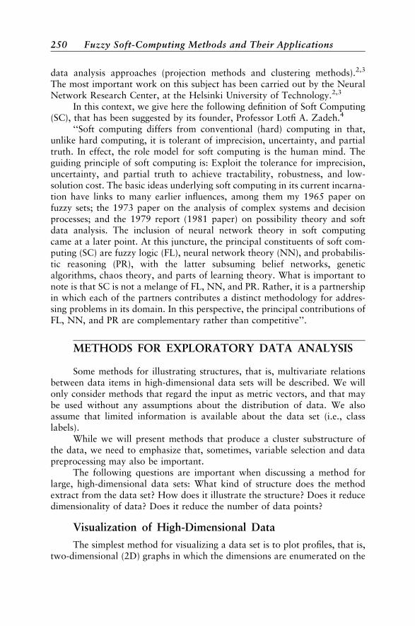
data analysis approaches (projection methods and clustering methods).2,3

The most important work on this subject has been carried out by the NeuralNetwork Research Center, at the Helsinki University of Technology.2,3

In this context, we give here the following definition of Soft Computing(SC), that has been suggested by its founder, Professor Lotfi A. Zadeh.4

‘‘Soft computing differs from conventional (hard) computing in that,unlike hard computing, it is tolerant of imprecision, uncertainty, and partialtruth. In effect, the role model for soft computing is the human mind. Theguiding principle of soft computing is: Exploit the tolerance for imprecision,uncertainty, and partial truth to achieve tractability, robustness, and low-solution cost. The basic ideas underlying soft computing in its current incarna-tion have links to many earlier influences, among them my 1965 paper onfuzzy sets; the 1973 paper on the analysis of complex systems and decisionprocesses; and the 1979 report (1981 paper) on possibility theory and softdata analysis. The inclusion of neural network theory in soft computingcame at a later point. At this juncture, the principal constituents of soft com-puting (SC) are fuzzy logic (FL), neural network theory (NN), and probabilis-tic reasoning (PR), with the latter subsuming belief networks, geneticalgorithms, chaos theory, and parts of learning theory. What is important tonote is that SC is not a melange of FL, NN, and PR. Rather, it is a partnershipin which each of the partners contributes a distinct methodology for addres-sing problems in its domain. In this perspective, the principal contributions ofFL, NN, and PR are complementary rather than competitive’’.

METHODS FOR EXPLORATORY DATA ANALYSIS

Some methods for illustrating structures, that is, multivariate relationsbetween data items in high-dimensional data sets will be described. We willonly consider methods that regard the input as metric vectors, and that maybe used without any assumptions about the distribution of data. We alsoassume that limited information is available about the data set (i.e., classlabels).

While we will present methods that produce a cluster substructure ofthe data, we need to emphasize that, sometimes, variable selection and datapreprocessing may also be important.

The following questions are important when discussing a method forlarge, high-dimensional data sets: What kind of structure does the methodextract from the data set? How does it illustrate the structure? Does it reducedimensionality of data? Does it reduce the number of data points?

Visualization of High-Dimensional Data

The simplest method for visualizing a data set is to plot profiles, that is,two-dimensional (2D) graphs in which the dimensions are enumerated on the

250 Fuzzy Soft-Computing Methods and Their Applications

x axis, with the corresponding values on y. An alternative, also widely used, isto plot 2D representations of pairs of two original dimensions. There are alsomethods that produce different curves based on the data points values, forexample, the components of data vectors are used as coefficients of orthogonalsinusoids, which are then added together. The most important drawback ofsuch methods is that they do not reduce the amount of data, and thus it cannotbe used effectively with large, high-dimensional data sets. However, they canbe used for illustrating data summaries.

Clustering Methods

The goal of clustering is to reduce the amount of data by groupingdata in classes so that similar items are grouped together and any two itemsfrom different classes are less similar than any two items from the same class.Clustering methods can be categorized as one of two types: hierarchical andpartitional clustering.

The hierarchical clustering methods are either agglomerative (i.e., themethods successively merge small clusters into larger ones), or divisive (i.e.,the methods successively split large clusters into smaller ones). The methodsdiffer in the rule used for merging or splitting clusters, the possibility to usevariate metrics, and so on.

Partitional clustering methods attempt to directly decompose a data setinto a fixed number of disjoint clusters. The methods attempt to minimize acriterion function, typically based on minimizing the dissimilarity insideclasses, while maximizing the dissimilarity between different classes.

Because of its relationship to SOM, we will describe in greater detailthe K-means clustering algorithm. The criterion function is the total squareddistance of the data items to their nearest cluster centroids,

EK ¼X

k

jxk � mcðxkÞj2 ½1�

where cðxkÞ is the index of the centroid closest to data item xk.There are two algorithms for computing the optimal set of classes. The

off-line original version, which requires access to all input vectors, follows:

1. Initialize the set of centroids, mi, i ¼ 1; . . . ;K.2. Assign each data item to the nearest class.3. Recompute the class centroids.4. If the difference between the new value of the criterion function E and its

old value is small enough, then stop; otherwise, go to Step 2.

The on-line variation of this algorithm, which needs only one input vector at atime, follows:

1. Initialize the set of centroids, mi, i ¼ 1; . . . ;K.2. Choose a randomly chosen data item.

Methods for Exploratory Data Analysis 251

3. Assign this data item to the nearest class.4. Recompute the selected class centroid.5. If the difference between the new value of the criterion function E and its

old value is small enough, then stop; otherwise go to Step 2.

The K-means clustering algorithm has a few problems, which have beendiscussed in Reference 5. One problem is the selection of different geometricalprototypes, and the use of suitable dissimilarity functions for them. While var-iations of this algorithm are available that use line prototypes, or convex com-binations between points and lines, it may also be the case that differentclusters of the data set have different shapes, and we need a mechanism todetermine the optimal prototype for each cluster. Another important problemis the a priori choice of the number K of classes. While validity functionalsexist that may be used to determine the number of clusters that produce thebest results, this approach has two main problems: first, the need to applythe algorithm for a whole range of possible values of K may, thus, miss theoptimal value; and, second, the functionals implicitly depend on the numberK. A method is needed to produce the optimal number of classes. A solution isto use a hierarchical approach in which, at each node of the binary tree a var-iation of the K-means algorithm is used to split a class into two subclasses. Thedecision about whether to split a class or not is based on a polarization index.Another problem relates to the possibility of clustering algorithms based oncrisp sets to identify isolated points and bridges between classes, and to dealwith overlapping classes. These problems are naturally solved by using cluster-ing algorithms based on fuzzy sets theory.

An approach based on clustering methods has the problem that the clus-ter prototype is as high dimensional as the original data set, and additionalvisualization methods are needed to visualize the data. While this is generallynot a problem, it becomes important when the data set is large and highlydimensional, as is the case with text mining problems.

Projection Methods

The main feature of clustering algorithms is that they reduce the amountof data cases by grouping them into classes. The projection methods describedbelow can be used for reducing the data dimensionality. The goal of these tech-niques is to represent the data set in a lower-dimensional space in such a waythat certain properties of the data set are preserved as much as possible.

Linear Projection Methods

The most widely used algorithm in this class is the principal componentanalysis (PCA) algorithm. It can be used to display the data as a linear projec-tion on a subspace of the original data space that best preserves the variance inthe data. The algorithm computes the principal components, which are the


orthogonal axes that show the maximal spread of the data, and considers thedata set as represented using coordinate axes given by the principal compo-nents. The most relevant principal components, based on the data variance,are selected and the data are projected onto the space represented by thoseorthogonal components.

Nonlinear Projection Methods

Alternate projection methods aim to reduce the data dimensionality byoptimizing the representation in the lower-dimension space so that the dis-tances between points in the projected space are as similar as possible to thedistances between the corresponding points in the original space. We willdescribe here a class of methods known as multidimensional scaling(MDS).6,7 The aim of these methods is to project data from a pseudo-metricspace (i.e., one characterized by a dissimilarity measure) onto a metric space.Such methods are especially useful for preprocessing non-metric data in orderto use algorithms valid only for metric input.

The first MDS method is the metric MDS, characterized by minimizingthe squared error cost function:

EM ¼Xk 6¼l

ðdðk; lÞ � d0ðk; lÞÞ2 ½2�

where, for the original items xk and xl, d(k,l) is their dissimilarity,6–12 andd’(k,l) is the distance between the corresponding vectors from the projectedmetric space. If the components of the data vectors are expressed on an ordinalscale, a perfect reproduction of the Euclidean distances may not be thebest goal. In such a situation, only the rank order of the distances betweenthe vectors is meaningful. The error function is defined as

EN ¼P

k 6¼l ðf ðdðk; lÞÞ � d0ðk; lÞÞ2Pk 6¼l ðd0ðk; lÞÞ2

½3�

where f is a monotonically increasing function that acts on the original dis-tances and always maps the distances to such values that best preserve therank order.

Another nonlinear mapping method, the Sammon’s mapping, is closelyrelated to the metric MDS. The only difference is that the errors in distancepreservation are normalized with the distance in the original space. Thus, pre-servation of small distances is emphasized. The error function is defined as

ES ¼Xk 6¼l

dðk; lÞ � d0ðk; lÞð Þ2

dðk; lÞ ½4�

Methods for Exploratory Data Analysis 253

ARTIFICIAL NEURAL NETWORKS

A neural network is an interconnected assembly of simple processing ele-ments, called units or nodes, whose functionality is loosely based on the ani-mal neuron. The processing ability of the network is stored in the interunitconnection strengths, called weights, obtained by a process of adaptation to,or learning from, a set of training patterns.13,14 In the following sections, wewill present the simplest neural network, the perceptron of Rosenblatt. Wewill continue with some of the most widely used types of neural networks:the multilayer network with feedforward and backpropagation of errors, theassociative memories, and the self-organizing maps. We will end with a discus-sion of other types of neural networks.

Perceptron

The perceptron of Rosenblatt is represented in Figure 1. The signalsx1; . . . ; xs appear as its input. Each input signal xi is weighted by the corre-sponding weight wi, and all these weighted inputs are then summed to calcu-late the activation value, which is then passed as the argument of an activationfunction f, to determine the neuron’s output value:13

o ¼ f ðwTx þ wsþ1Þ ¼ fX

j

wjxj þ wsþ1

!½5�

The learning problem is to find the weights vector w 2 Rsþ1 such that thecomputed output of the unit, ok 2 R, is as close as possible, if not equal, to thedesired output, yk 2 R, for all the available input vectors xk. The activation

w1U

1

x1

wiUi

x1

wsU

s

xs

f 0

1

ws+1

+

Figure 1 The perceptron of Rosenblatt.


function f may have different forms. In the perceptron of Rosenblatt case, f isdefined as

f ðxÞ ¼ 1 if x>00 otherwise

�½6�

Other variations of the perceptron use an identical activation function,that is, f ðxÞ ¼ x. The mathematical interpretation of the original perceptronis the problem of linear separability of two classes. The original conditionof linear separability is to find a weight vector w such that wT xk>0 for allpoints xk in one class, and wT xk>0 for all points xk in the other class.With a suitable linear transformation, the separability condition becomeswTxk<0 for all the points xk correctly classified, and wTxk<0 otherwise.This means that in the case of the Rosenblatt perceptron, the desired outputvalue yk is always 1. The training procedure is the following:

1. Arbitrarily initialize the weights vector w.2. Feed a test input vector xk to the neuron.

a. If the output value ok and the desired value yk match, do nothing.b. If they do not match, then change the values of the weights vector in

some way, in order to improve the behavior of the neuron.

3. Repeat Step 2 for all the test vectors available, until no improvement isdone for all the test vectors, or until a certain maximal number of iterationshas been reached.

The correction realized at Step 2(b) is determined from the error minimi-zation condition, and is called the perceptron learning rule:

w : ¼ w þ c � ðyk � okÞ � xk ½7�

Throughout this chapter, the notation w : ¼ denotes the process ofevaluation of the given expression and assignment of the produced value tothe variable w.

The original perceptron of Rosenblatt works with the desired outputvalues yk ¼ 1, the computed output values ok 2 f0; 1g, and the activationfunction as defined above. Even if this algorithm has been proven to convergein a limited number of steps if a separation hyperplane does exist, this parti-cular set of parameters is not the most suitable. First, the separation hyper-plane produced is not the best one, but, instead, it is very near one of theclasses. Second, this algorithm does not work when a separation hyperplanedoes not exist. The generalizations of this algorithm allow a differentchoice of desired values and activation function, and aim to solve both pro-blems. Another feature is the way the test in Step 2 (a) is done. In most cases,it is carried out as described above, that is, a single test, for the current inputvector, is made for each iteration. These algorithms are called on-line learning


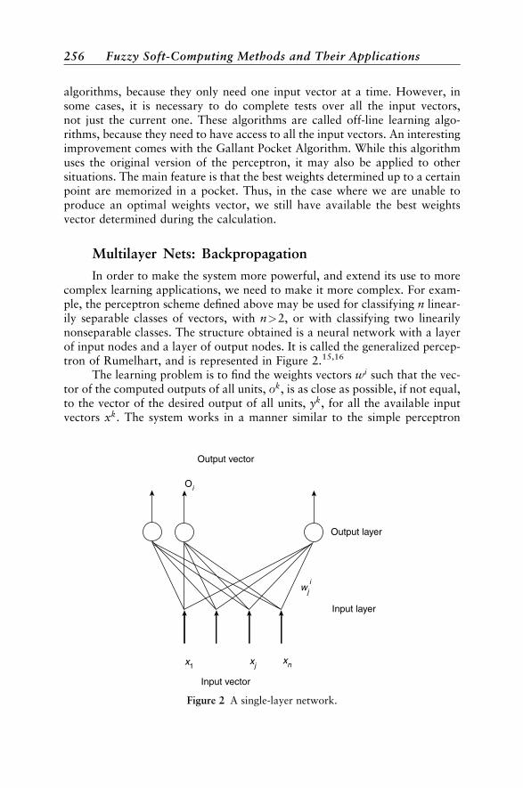
algorithms, because they only need one input vector at a time. However, insome cases, it is necessary to do complete tests over all the input vectors,not just the current one. These algorithms are called off-line learning algo-rithms, because they need to have access to all the input vectors. An interestingimprovement comes with the Gallant Pocket Algorithm. While this algorithmuses the original version of the perceptron, it may also be applied to othersituations. The main feature is that the best weights determined up to a certainpoint are memorized in a pocket. Thus, in the case where we are unable toproduce an optimal weights vector, we still have available the best weightsvector determined during the calculation.

Multilayer Nets: Backpropagation

In order to make the system more powerful, and extend its use to morecomplex learning applications, we need to make it more complex. For exam-ple, the perceptron scheme defined above may be used for classifying n linear-ily separable classes of vectors, with n>2, or with classifying two linearilynonseparable classes. The structure obtained is a neural network with a layerof input nodes and a layer of output nodes. It is called the generalized percep-tron of Rumelhart, and is represented in Figure 2.15,16

The learning problem is to find the weights vectors wi such that the vec-tor of the computed outputs of all units, ok, is as close as possible, if not equal,to the vector of the desired output of all units, yk, for all the available inputvectors xk. The system works in a manner similar to the simple perceptron

Oi

Output layer

Input layer

Input vector

Output vector

x1 xjxn

wji

Figure 2 A single-layer network.


described above. One input vector is passed to the net at each iteration. Byusing the weights and the activation function, which in this case is also linear,the output values of all the nodes are computed. These values are then com-pared with the desired values for these nodes. For all the nodes that show amismatch between the computed and the desired values, we need to changethe weights to improve the behavior of the system. The correction rule usedin this case is determined by minimizing the error function. But, as opposedto the perceptron where the minimization was done on the output values, inthis case the minimization is done on the activation values. The correction ruleused here is called the delta rule:

wi : ¼ wi þ c � ðyki � ok

i Þ � xk ½8�

where yki and ok

i are the desired output value and computed output value cor-responding to the ith output unit. Again, the input vector is xk, and wi is theweights vector of the ith output node.

The rule described above may be further generalized so that it may beapplied to the training of a more complex type of network, which containsso-called hidden layers of neurons. Here we have a multilayer net with back-propagation, so-called because of the way the error is propagated backwardfrom the output layer to the input layer. This network is presented inFigure 3. We use the following notations: For an input vector x, xi is the value

Hidden layer

Output layer

Input layer

Input vector

Output vector

wji

wkj

k

j

i

Figure 3 Multilayer neural network with feedforward and error backpropagation.


given at the ith input unit, wji is the weight of the connection from the ith inputunit to the jth hidden unit, wkj is the weight of the connection from the jthhidden unit to the kth output unit, fj is the activation function of the jth hiddenunit, netj is the activation value of the jth hidden unit, oj ¼ fj(netj) is the com-puted output value of the jth hidden unit, and fk, netk, and ok have a similarmeaning for the kth unit of the output layer. Finally, yk is the desired outputvalue for the kth unit of the output layer.

The generalized delta rule for the kth output unit is given by

wkj : ¼ wkj þ cdkoj ½9�

where

dk : ¼ ðyk � okÞf 0kðnetkÞ ½10�

Similarly, the same rule for the jth hidden unit is given by

wji : ¼ wji þ cdjxi ½11�

where

dj : ¼X

k

dkwkj

!f 0j ðnetkÞ ½12�

Note that the d values on an internal node may be computed based on the dvalues of the superior nodes, which is the theoretical reason for evaluating inthe first place the errors of the output layer, and later propagating these errorsbackward to the input layer.

A typical activation function is the sigmoidal function, that is, f ðxÞ ¼1=ð1 þ e�x). In this case, f 0ðxÞ ¼ f ðxÞ � ð1 � f ðxÞÞ, and we have

dk : ¼ ðyk � okÞokð1 � okÞ ½13�

and

dj : ¼X

j

dkwkj

!ojð1 � ojÞ ½14�

The learning algorithm of this network is the following:

1. Present the pattern to the input layer.2. Let the hidden units evaluate their output using the pattern.3. Let the output units evaluate their output using the result in Step 2.4. Calculate the dk values for the nodes of the output layer.


5. Train each output node using the generalized delta rule and the dk valuesfrom Step 4.

6. Calculate the dj values for the nodes of the hidden layer.7. Train each hidden node using the generalized delta rule and the dj values

from Step 6.

Steps 1–3 are known as the forward pass, while Steps 4–8 are known asthe backward pass.

Associative Memories: Hopfield Net

The Hopfield neural network is a simple artificial network, able to storecertain memories so that the full pattern can be recovered if the network ispresented with only partial information. Furthermore, there is a degree of sta-bility in the system—if just a few connections between nodes (neurons) are sev-ered, the recalled memory is not too badly corrupted—the network canrespond with a ‘‘best guess’’.13 The nodes in the network are vast simplifica-tions of real neurons—they can exist only in one of two possible ‘‘states’’—fir-ing or not firing. Every node xi is connected to every other node xj with somestrength wij, such that wij ¼ wji and wii ¼ 0. At any instant of time, a node willchange its state (i.e., start or stop firing) depending on the inputs it receivesfrom the other nodes. The values of these neurons are thus binary, meaningthat xi 2 f0; 1g. If the system is initialized with any general pattern of firingand nonfiring nodes, then this pattern will generally change with time. Tosee this, think of starting the network with just one firing node. Thiswill send a signal to all the other nodes via its connections so that a shorttime later some of these other nodes will fire. These new firing nodes willthen excite others after another short time interval and a whole cascade of dif-ferent firing patterns will occur. One might imagine that the firing pattern ofthe network would change in a complicated, perhaps random, way with time.The important property of the Hopfield network that renders it useful forsimulating memory recall is the following: One is guaranteed that the patternwill settle down after a long enough time to some fixed pattern. Certain nodeswill always be ‘‘on’’ and others always ‘‘off’’. Furthermore, it is possible toarrange that these stable firing patterns of the network correspond to thedesired memories we wish to store. The total input of a certain neuron i,Hi, comes from the external input Ii and from other neurons. Thus,

Hi : ¼Xj6¼i

wijxj þ Ii ½15�

When the outputs of the neurons are updated, the output value of neuron i is

xi : ¼0 if Hi<Ui

1 if Hi>Ui

�½16�


where Ui is the threshold value of the neuron i. We need to update the weightswij so that the system is able to memorize a set of energy-stable states xs,s ¼ 1; 2; . . . . The produced algorithm is the following:

A. Memorization. To memorize the set of binary vectors xs, s ¼ 1; 2; . . ., set

wij ¼X

s

ð2xsi � 1Þð2xs

j � 1Þ

wii ¼ 0

½17�

B. Recognition.

1. For the input vector x0, evaluate

H0i ¼

Xj

wijð2x0j � 1Þ ½18�

2. Update x0

xi ¼0 if H0

i<Ui

1 if H0i>Ui

�½19�

3. If �x0i ¼ 0, 8i, then stop, otherwise, continue from Step 2.

Note that it has theoretically been proven that a Hopfield network with nnodes may accurately recognize a maximum of n/(2 log n) patterns. This gives11 patterns for a network with 100 nodes.

Self-Organizing Map

The SOM is an artificial neural network used to visualize and interpretlarge high-dimensional data sets. Typical applications are visualization of pro-cess states or financial results by representing the central dependencies withinthe data on the map.1,2 The SOM is a method that can be used both to reducethe amount of data by clustering, and to project the data nonlinearly onto alower-dimensional display. The map consists of a regular grid of processingunits, the ‘‘neurons’’. A model of some multidimensional observation, even-tually a vector consisting of features, is associated with each unit. The mapattempts to represent all the available observations with optimal accuracyusing a restricted set of models. At the same time, the models become orderedon the grid so that similar models are close to each other and dissimilar modelsare far from each other. Fitting of the model vectors (also called referencevectors) is usually carried out by a sequential regression process, wheret ¼ 1,2, . . ., is the step index. For each sample x(t), first the winner index c(best match) is identified by the condition

jxðtÞ � mcðtÞj � jxðtÞ � miðtÞj for all i ½20�


After that, all model vectors or a subset of them that belong to nodescentered around node c ¼ cðxÞ are updated as

miðt þ 1Þ ¼ miðtÞ þ hciðtÞðxðtÞ � miðtÞÞ ½21�

Here, hci is the neighborhood function, a decreasing function of the distancebetween the ith and cth nodes on the map grid. The regression is usually iter-ated over the available samples. In practice, the neighborhood area is chosento be wide in the beginning of the learning process, and both its width andheight will decrease during learning.

Properties

Ordered DisplayAs the data items are mapped to those units on the map that have the

closest reference vectors, nearby units will have similar data items mappedon them. This property requires that the map be regarded as an ordered dis-play, which facilitates the understanding of the structures in the data set. Thismap display may also be used as an ordered groundwork, on which the origi-nal data variables, as well as other information related to the data cases, maybe displayed.

Cluster VisualizationThe ordered display might be used for showing the clustering density in

different regions of the data space. The density of the reference vectors of anorganized map will reflect the density of the input samples. The cluster displaymay be constructed as follows: the distance between each pair of neighboringreference vectors is scaled so that it fits between a given minimum and max-imum value. Each scaled distance value determines the gray level of the pointbeing situated in the middle of the segment line determined by the correspond-ing map units. The gray level of the points corresponding to the map unitsthemselves are set to the average of some of the nearest distance values. Afterthese values have been set up, they may be smoothed and then visualized.

Missing DataAn interesting feature of the SOM is its ability to deal with missing data.

Some of the components of the data vectors may not be available for all dataitems, or may not be applicable or defined. The simplest solution when dealingwith such incomplete components would be to discard the incomplete vari-ables or incomplete data items completely, but in this way we will lose usefulinformation. In the case of the SOM, the problem of missing data may be trea-ted as follows: When choosing the winning unit, the input vector can be com-pared with the reference vectors mi using only those components that are


available in x. When the reference vectors are then adapted, only the compo-nents that are available in x will be modified. This approach produces betterresults than by discarding data from the data set.

OutliersThe outliers are data items situated very far from the main body of data.

This may be due to measurement errors, typographical errors, or may simplybe correct data that is strikingly different from the rest. In the case of the mapsgenerated by the SOM, each outlier affects only one map unit and its neighbor-hood, while the rest of the map is available for the rest of the analysis. Further-more, the outliers can be detected in the map due to the much lower density ofthe space near them.

Mathematical Characterization

Rigorous mathematical proof of the SOM algorithm is very difficult ingeneral. In the case of a discrete data set and a fixed neighborhood function,the error function of the system may be defined as

E ¼X

k

Xi

hcijxk � mij2 ½22�

where the index c depends on the data item xk and the reference vectors mi.The learning rule of the SOM corresponds to a gradient descent step in mini-mizing the sample function

E1 ¼X

i

hcijxðtÞ � mij2 ½23�

obtained by a random selection of a sample x(t) at iteration t. The cost func-tion of the SOM closely resembles the objective function of the K-means clus-tering algorithm: In the SOM, the distance of each input to all the referencevectors is taken into account, weighted by the neighborhood kernel h, whilein the K-means algorithm, only the distance to the closest centroid is used.The cost function of the SOM can be decomposed to two terms as follows:

E ¼X

k

jxk � ncj2 þX

i

Xj

hijNijni � mjj2 ½24�

where Ni is the number of the data items closest to the reference vector mi, andni is the weighting center of the same data items, with the assumption thatP

j hij ¼ 1 for all values of i. The first term in the relation above is the objectivefunction of the K-means clustering algorithm. However, here the clusters arenot defined in terms of their centroids ni, but in terms of the reference vectors


mi. With respect to the second term, note that ni and mi will generally be closeto each other, since ni is the centroid of the cluster defined by mi.

Relation between SOM and MDS

When computing the index of the closest unit to the input vector, theEuclidean distance was used. This is not a restriction, as one may use anytype of distance. If there is only a dissimilarity (i.e., pseudo-metric) available,we need to create a space where a distance can be defined that preserves asmuch as possible the original dissimilarities. The techniques used for that pur-pose are the MDS methods described in a previous section. Since different dataanalysis methods display different properties of the data set, the most usefulapproach is to use several methods together. A possible combination is to firstreduce the amount of data either by clustering or by the SOM, and thento display the reference vectors with some distance-preserving projectionmethod, to gain additional insight.

Multiple Views of the SOM

The SOM is a model that emphasizes particular aspects of biologicalneural nets, especially those ordered ‘‘maps’’ found experimentally in the cor-tex. The SOM captures some of the fundamental processing principles of thebrain. The SOM is a model of unsupervised machine learning and also anadaptive knowledge representation scheme. The SOM is a tool for statisticalanalysis and visualization. The SOM is both a projection method that mapshigh-dimensional data space into low-dimensional space, and a clusteringmethod in which similar data samples tend to be mapped to nearby neurons.

There exist a number of variants of the SOM in which the adaptationrules are different, various distance measures may be used, and the structureof the map interconnections is variable. The SOM is a tool for the develop-ment of complex applications. The SOM is widely used as a data miningand visualization method for complex data sets. Applications areas includeimage processing, speech recognition, process control, economical analysis,and diagnostics in industry and medicine.1–3 Searching the best-matchingunit is usually the computationally heaviest operation in the SOM. A wayto deal with this is to build a hierarchy of SOMs, teaching the SOM oneach level before proceeding to the next layer. Most SOM applications usenumerical data. Statistical features of natural text can also be regarded asnumerical features that facilitate applications of SOM in apparently nonnume-rical contexts.

Other Architectures

The field of artificial neural networks is very large. A large numberof different neural networks architectures have been developed.17 Recurrent


networks deserve a special mention here. They allow participating nodes tosimultaneously receive and transmit signals; in this way, no distinction ismade between input and output nodes. Some of the nodes, the visible nodes,allow an interface with the environment. As in the feedforward network,there are also hidden nodes, which do not allow such interaction. Another var-iation among neural networks is related to the way the weights are updated. Inan extreme case, all the weights are changed at once. At the other extreme, theweights are updated sequentially, one neuron at a time. These are particularexamples of a more general case in which the weights of the neurons areupdated periodically with a certain probability, and on an individual basis.

EVOLUTIONARY ALGORITHMS

Evolutionary Algorithms are search and optimization procedures thathave their origin and inspiration in the biological world: The theory of evolu-tion, based on the idea of survival of the fittest in a dynamic environment.18

Evolutionary algorithms are based on the learning process within a populationof individuals, each of which represents a point in the solution search space ofa certain problem. The population is arbitrarily initialized, and it evolvestoward better regions of the search space by means of randomized processesof selection (which favors the reproduction of better individuals), recombina-tion (which allows the mixing of parental information when passing it tothe descendants), and mutation (which allows some random innovation tobe introduced into the population, in order to prevent premature convergenceto local optima). Considering the aim of the search, the problem offers a fitnessvalue of the search points, as an indication of their closeness to the solution.Each evolutionary step is called a generation. A pseudo-code of the genericevolutionary algorithm (EA) is the following:

// start with an initial time

t : ¼ 0

// initialize a random population of individuals

initpopulation P(t)

// evaluate fitness of individuals in initial population

evaluate P(t)

// test for termination criterion (time, fitness, etc.)

while not done do

// increase the time counter

t : ¼ t þ 1

// select subpopulation for reproduction

P0 : ¼ selectparents P(t)


// recombine the genes of selected parents

recombine P0(t)

// perturb the mated population

mutate P0(t)

// evaluate its new fitness

evaluate P0(t)

// select the survivors based on the fitness

P : ¼ select P, P0(t)

end while

end EA

Evolutionary algorithms, as simulations of genetic processes, are not ran-dom searches for a solution of a problem. Evolutionary algorithms use sto-chastic processes, but the result is distinctly nonrandom. The most widelyused types of evolutionary algorithms, which have developed independently,are genetic algorithms, evolution strategies, and evolutionary programming,which will be discussed in the following sections. As we will see, they differin the way the individuals are represented, in what genetic operators theyuse, and in how they are defined.

GENETIC ALGORITHMS

The genetic algorithm (GA) model of computation, as created byHolland in 1975, and referred to as the canonical GA, has some distinct par-ticularities.19 These include representation, fitness function, and others, whichwill now be discussed.

Canonical GA

RepresentationCanonical GA considers the individuals in the population to be fixed

length arrays of bits. Simple bit manipulation operations allow the implemen-tation of genetic operators. In order to apply the canonical GA to optimizationproblems, the bit string is logically divided into segments. Each segment is theninterpreted as the binary code of the corresponding optimization variable.There are many segment decoding functions, the simplest one being the simplebinary representation of integer values that, if necessary, are combined with ascaling from a certain real interval to a suitable integer interval.

Fitness FunctionDifferent fitness functions are obtained based on the original objective

function, on the individual decoding function (produced by combining the

Genetic Algorithms 265

segment decoding functions), and on a scaling function aimed at generatingpositive fitness values, higher for better individuals.

SelectionSelection of the next generation of parents is made with respect to the

probability distribution based on fitness values. The fitness values for eachindividual are computed. Based on the relative fitness of an individual to thetotal fitness of the population, the probabilities of selection of individuals arecomputed. Then, the cumulative probability for each individual is computedas the sum of probabilities of selection of individuals with a smaller index.The new generation is selected based on generating random numbers in therange [0,1] and on matching them to the cumulative probabilities. Obviously,some individuals will be selected more than once, but this is the intended beha-vior: The best individuals get more copies, the average stays fixed, and theworst die off.

RecombinationThis quantity is an operator working entirely on bit representations and

completely ignoring the logical segments representing the optimized variables.Based on the probability given by the crossover rate, pc, a number of parents israndomly selected. From this set of parents, pairs of parents are also randomlyselected. Suppose that two parent individuals, u ¼ ðu1;u2; . . . ; ulÞ andv ¼ ðv1; v2; . . . ; vlÞ have thus been selected for the crossover. There are morecrossover operators to be applied here. The one-point crossover operatorselects at random a crossing point, and generates two offspring from thetwo parents: u0 ¼ ðu1; . . . ; ui; viþ1; . . . ; vlÞ and v0 ¼ ðv1; . . . ; vi; uiþ1; . . . ; ulÞ.These offspring will replace the parents in the population. This may be gener-alized to the m-point crossover by using more than one breakpoint. Anotheroption is the uniform crossover, which uses a randomly generated maskfor deciding, for each bit, whether to exchange information between parentsor not.

MutationThis operator works on the bit string level, and is considered a back-

ground operator. It inverts single bits of individuals with a very small prob-ability pm, � 0.001. The practical implementation of this probability maybe done via generating a random real number in the interval [0,1]. If the num-ber is smaller than the given probability, the mutation operation is realized ona bit, also randomly generated.

Evolution Strategies

The first Evolution Strategy (ES) was developed in 1964 at the TechnicalUniversity of Berlin, as an experimental optimization technique. This variant,


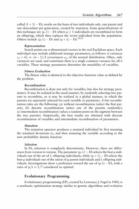
called (1 þ 1Þ � ES, works on the basis of two individuals only, one parent andone descendant per generation, created by mutation. Some generalizations ofthis technique are (m; 1Þ � ES where m � 1 individuals are recombined to forman offspring, which then replaces the worst individual from the population.Others include ðm; lÞ � ES and (mþ lÞ � ES.20,21

RepresentationSearch points are n-dimensional vectors in the real Euclidean space. Each

individual may include additional strategy parameters, as follows: n variancescii ¼ s2

i , n � ðn � 1Þ=2 covariances cij, of the normal distribution. Often, onlyvariances are used, and sometimes there is a single common variance for all nvariables. These strategy parameters determine the mutability of variables.

Fitness EvaluationThe fitness value is identical to the objective function value as defined by

the problem.

RecombinationRecombination is done not only for variables, but also for strategy para-

meters. It may be realized in the usual manner, by randomly selecting two par-ents to recombine, or it may be realized in a global manner, in which theparents are separately selected for each variable or parameter. A few recombi-nation rules are the following: (a) without recombination (select the first par-ent); (b) discrete recombination (select one of the parents randomly);(c) intermediate recombination (select a random point on the segment betweenthe two parents). Empirically, the best results are obtained with discreterecombination of variables and intermediate recombination of parameters.

MutationThe mutation operator produces a mutated individual by first mutating

the standard deviations si, and then mutating the variable according to thenew probability density function.

SelectionIn ES, selection is completely deterministic. However, there are differ-

ences from version to version. The parameter (m; lÞ � ES selects the best m indi-viduals out of the set of l offspring individuals, while ðmþ lÞ � ES selects thebest m individuals out of the union of m parent individuals and l offspring indi-viduals. Investigations show a preference toward the use of (m l) � ES, with aratio of m=l � 1=7 considered as optimal.

Evolutionary Programming

Evolutionary programming (EP), created by Lawrence J. Fogel in 1960, isa stochastic optimization strategy similar to genetic algorithms and evolution

Genetic Algorithms 267

strategies, but places the emphasis on the link between parent and offspring,instead of emulating specific genetic operators.22 Combinatorial and real-valued function optimization problems having many locally optimal solutionsare well suited for this technique.

RepresentationInitially, the variables are vectors from a bounded subspace of Rn. After-

wards, the search domain is extended to the whole space. The Meta-evolution-ary programming approach also incorporates strategy parameters (standarddeviations) in this representation.

Fitness EvaluationThe fitness values are obtained from objective function values by scaling

to positive values and possibly by imposing a random alteration.

RecombinationNo recombination operator combining features of different individuals is

used with EP. In EP, individuals are viewed as species, and distinct species donot recombine.

MutationEach individual is replicated into a new population. Each offspring is

mutated according to a distribution of mutation types, from minor to extreme.The severity of mutations is often reduced as the global optimum isapproached.

SelectionThe new population is selected via a stochastic q-tournament selection.

For each individual from PðtÞ [ P0ðtÞ, q individuals are randomly selected fromthe same set, and compared to the original individual, determining its score.The individuals with the highest score form the new population. There is nolimitation in the number of offspring produced by an individual. Also, there isno limitation in keeping the population size constant.

FUZZY SETS AND FUZZY LOGIC

The mathematics of Fuzzy Set Theory was originated by L. A. Zadeh in1965.4 It deals with the uncertainty and fuzziness arising from interrelatedhumanistic types of phenomena such as subjectivity, thinking, reasoning, cog-nition, and perception. This approach provides a way to translate a linguisticmodel of the human thinking process into a mathematical framework fordeveloping the computer algorithms for computerized decision-making pro-cesses.4,23–27 On the other hand, a fuzzy set is a generalized set to whichobjects can belong with various degrees (grades) of memberships over the


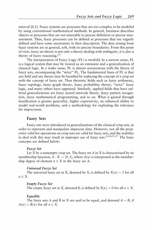
interval [0,1]. Fuzzy systems are processes that are too complex to be modeledby using conventional mathematical methods. In general, fuzziness describesobjects or processes that are not amenable to precise definition or precise mea-surement. Thus, fuzzy processes can be defined as processes that are vaguelydefined and have some uncertainty in their description. The data arising fromfuzzy systems are in general, soft, with no precise boundaries. From this pointof view, fuzzy set theory is not only a theory dealing with ambiguity, it is also atheory of fuzzy reasoning.23

The interpretation of Fuzzy Logic (FL) is twofold. In a narrow sense, FLis a logical system that may be viewed as an extension and a generalization ofclassical logic. In a wider sense, FL is almost synonymous with the theory offuzzy sets, encompassing the ‘‘strict’’ FL. The fundamental basis of FL is thatany field and any theory may be fuzzified by replacing the concept of a crisp setwith the concept of fuzzy set. Thus theoretic fields such as fuzzy arithmetic,fuzzy topology, fuzzy graph theory, fuzzy probability theory, ‘‘strict’’ fuzzylogic, and many others have appeared. Similarly, applied fields that have suf-fered generalizations are fuzzy neural network theory, fuzzy pattern recogni-tion, fuzzy mathematical programming, and so on. What is gained throughfuzzification is greater generality, higher expressivity, an enhanced ability tomodel real-world problems, and a methodology for exploiting the tolerancefor imprecision.

Fuzzy Sets

Fuzzy sets were introduced as generalizations of the classical crisp sets, inorder to represent and manipulate imprecise data. However, not all the prop-erties valid for operations on crisp sets are valid for fuzzy sets, and the inabilityto deal with this may result in improper use of fuzzy sets.4,14,23–27 The basicconcepts are defined below:

Fuzzy SetLet X be a nonempty crisp set. The fuzzy set A in X is characterized by its

membership function, A : X ! ½0; 1�, where A(x) is interpreted as the member-ship degree of element x 2 X in the fuzzy set A.

Universal Fuzzy SetThe universal fuzzy set in X, denoted by X, is defined by XðxÞ ¼ 1 for all

x 2 X.

Empty Fuzzy SetThe empty fuzzy set in X, denoted ;, is defined by ;ðxÞ ¼ 0 for all x 2 X.

EqualityThe fuzzy sets A and B in X are said to be equal, and denoted A ¼ B, if

AðxÞ ¼ BðxÞ for all x 2 X.

Fuzzy Sets and Fuzzy Logic 269

Fuzzy SubsetThe fuzzy set A in X is a subset of the fuzzy set B in X, denoted A � B, if

AðxÞ � B(x) for all x 2 X.

ComplementThe complement of a fuzzy set A in X, denoted A, is defined by

AðxÞ ¼ 1 � AðxÞ for all x 2 X.

IntersectionThe intersection of fuzzy sets A and B in X, denoted A\B is the fuzzy set

defined as ðA \ BÞðxÞ ¼ TðAðxÞ;BðxÞÞ for all x 2 X, where T is a triangularnorm (i.e., commutative, associative, nondecreasing in each argument, andTða; 1Þ ¼ a for all a 2 ½0; 1�).

UnionThe union of fuzzy sets A and B in X, denoted A [ B, is the fuzzy set

defined as ðA [ BÞðxÞ ¼ SðAðxÞ;BðxÞÞ, for all x 2 X, where S is a triangularconorm (i.e., commutative, associative, nondecreasing in each argument,and S(a; 0Þ ¼ a for all a 2 ½0; 1�).

In what follows, some of the properties of crisp sets will be analyzedfrom the point of view of applicability with fuzzy sets. We have listed theseproperties in Table 1 along with examples of two widely used t-norms andt-conorms:

Standard TSða; bÞ ¼ minfa; bg and SSða; bÞ ¼ maxfa; bgLukasiewicz TLða; bÞ ¼ maxfa þ b � 1; 0g and SLða; bÞ ¼ minfa þ b; 1g

1. Property 1 in Table 1 is satisfied only by the standard t-norm and t-conorm.2. Property 4 in Table 1 is satisfied by any t-norm and t-conorm.3. Any t-norm and t-conorm, defined on nondegenerate fuzzy sets, that satisfy

properties 2, do not satisfy property (3).4. For any t-norm and t-conorm that posses the properties 2 and 3, the fuzzy

sets have only crisp values, that is, they reduce to crisp sets.

Table 1 The Properties of Crisp Sets from the Point of View of Applicabilitywith Fuzzy Sets

Property Crisp Sets Ts and SS TL and SL

(1) Idempotence laws Valid Valid Invalid(2) A \ A ¼ ; and A [ A ¼ X Valid Invalid Valid(3) Distributivity laws Valid Valid Invalid(4) De Morgan laws Valid Valid Valid


The properties shown in Table 1 use the standard definition suitable foruse in ‘‘strict’’ FL, and the Lukasiewicz definition suitable for use in fuzzy clus-tering.

Fuzzy Logic

The basic assumption upon which two-valued logic is based, that everyproposition is either true or false, has been questioned since Aristotle.For example, propositions about future events are neither actually true, noractually false, but potentially either. Consequently, their truth-value isundetermined, at least prior to the event. Propositions whose truth-value isproblematic are not limited to future events. For example, propositions thatimply physical or chemical measurements depend on the limitations of mea-surement.23–27 While several types of multivalued logic have been proposed,here we will discuss the infinite-valued logic, whose truth-values are repre-sented by all the real numbers in the interval [0,1]. This is also called standardLukasiewicz logic L1. The primitives of this logic are defined as

�aa ¼ 1 � a

a ^ b ¼ minða; bÞa _ b ¼ maxða; bÞ

a ) b ¼ minð1; 1 þ b � aÞa , b ¼ 1 � ja � bj

½25�

It can be verified that the relations above reduce to their usual counter-parts when applied to binary logic. The standard Lukasiewicz logic L1 is iso-morphic to fuzzy set theory based on the standard fuzzy operations in the sameway the two-valued logic is isomorphic to the crisp set theory. The member-ship degree A(x) for x 2 X may be interpreted as the truth value of the propo-sition ‘‘x is a member of the set A’’. The reciprocal is also valid.

Fuzzy PropositionsThere are four types of fuzzy propositions. Unconditional and unquali-

fied propositions are of the form

p : V is F ½26�

where V is a variable that takes values from a universe V of values, and F is afuzzy set on V that represents a fuzzy predicate (e.g., tall, large, high). Thedegree of truth of this proposition is defined as TðpÞ ¼ FðvÞ, for each givenparticular value v of variable V. Unconditional and qualified propositionsare of the form

p : V is F is S ½27�


where S is a fuzzy truth qualifier (e.g., fairly true, very false, etc.). The degreeof truth of this proposition is defined as TðpÞ ¼ SðFðvÞÞ, for each given parti-cular value v of variable V. Conditional and unqualified propositions are of theform

p : If X is A then Y is B ½28�

where X and Y are variables with values in X, Y and A and B are fuzzy setson X, Y. This proposition may be viewed as hX;Yi is R, where R is a fuzzyset on X � Y. The degree of truth of this proposition is defined asTðpÞ ¼ Rðx; yÞ ¼ JðAðxÞ, B(y)), for each given particular values x, y of vari-ables X, Y. The parameter J denotes the fuzzy implication operation. Condi-tional and qualified propositions are of the form

p : If X is A; thenY is B is S ½29�

Its truth-value is determined in a way similar to the cases above.

Fuzzy QuantifiersFuzzy quantifiers are fuzzy numbers that take part in fuzzy propositions.

They are of the following two kinds. Absolute quantifiers are defined on R(� 10, >100, at least � 5) and may be used in two forms of propositions:

p : There are Q i0s in I such that VðiÞ is F

q : There are Qi0s in I such that V1ðiÞ is F1 and V2ðiÞ is F2

½30�

where V, V1, V2 are variables that take values from sets V, V1, V2, I is a setof individuals, Q is a fuzzy number on R, and F, F1, F2 are fuzzy sets on V, V1,V2. The truth-value of these sentences is defined as

TðpÞ ¼ Q

�Xi in I

FðVðiÞ�

TðqÞ ¼ Q

�Xi in I

minðF1ðV1ðiÞÞ; F2ðV2ðiÞÞ�

½31�

The latter case assumes the standard intersection of two fuzzy sets. Relativequantifiers are defined on [0, 1] (almost all, about half, most) and may beused in propositions of the form:

p : Among i0s in Isuch that V1ðiÞ is F1 there are Q i0s in I such that V2ðiÞ is F2

where Q is a fuzzy number on [0, 1]. The truth-value of this sentence is definedassuming the standard intersection of two fuzzy sets.


Linguistic HedgesThese are linguistic terms that modify other linguistic terms, for exam-

ple, very, more or less, fairly, extremely. They may be used to modify fuzzypredicates, fuzzy truth-values, and fuzzy probabilities. The fuzzy set thatdefines the hedge is called a modifier.

TðpÞ ¼ Q

Pi2I minðF1ðcalÞV1ðiÞÞ; F2ðcal V2ðiÞÞÞP

i2I F1ðcal V1ðiÞÞ

� �½32�

The modifier is simply applied over the fuzzy set associated with the predicate,value, or probability it modifies. For example, the proposition ‘‘x is young [istrue]’’ may be modified by the hedge very in the following ways:

* ‘‘x is very young is true’’

* ‘‘x is young is very true’’

* ‘‘x is very young is very true’’

Inference from Fuzzy PropositionsThe inference rules of crisp logic have been generalized in the framework

of fuzzy logic in order to facilitate approximate reasoning. Separate general-izations have been made for dealing with conditional fuzzy propositions (gen-eralized modus ponens, generalized modus tolens, generalized hypotheticalsyllogism), conditional and qualified propositions and quantified propositions.

Fuzzy Clustering

As is well known, Cluster Analysis involves the classification of objectsinto categories. Since most categories have vague boundaries, and may evenoverlap, the necessity of introducing fuzzy sets is obvious. A discussion ofFuzzy Clustering must refer to the following issues:5,28–37

Data RepresentationInput data is obtained from measurements on the objects that are to be

recognized. Each object is represented as a vector of measured valuesx ¼ ðx1; x2; . . . ; xsÞ, where xi is a particular characteristic of the object.

Feature ExtractionDue to the large number of characteristics, there is a need to extract the

most relevant characteristics from the input data, so that the amount of infor-mation lost is minimal, and the classification realized with the projected dataset is relevant with respect to the original data. In order to achieve this featureextraction, different statistical techniques, as well as the fuzzy clustering algo-rithms outlined here, may be used.


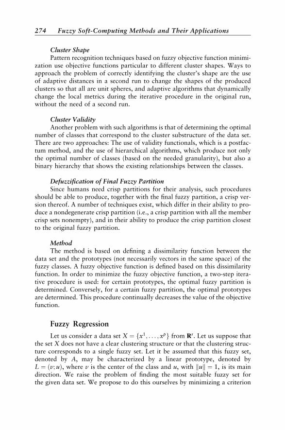
Cluster ShapePattern recognition techniques based on fuzzy objective function minimi-

zation use objective functions particular to different cluster shapes. Ways toapproach the problem of correctly identifying the cluster’s shape are the useof adaptive distances in a second run to change the shapes of the producedclusters so that all are unit spheres, and adaptive algorithms that dynamicallychange the local metrics during the iterative procedure in the original run,without the need of a second run.

Cluster ValidityAnother problem with such algorithms is that of determining the optimal

number of classes that correspond to the cluster substructure of the data set.There are two approaches: The use of validity functionals, which is a postfac-tum method, and the use of hierarchical algorithms, which produce not onlythe optimal number of classes (based on the needed granularity), but also abinary hierarchy that shows the existing relationships between the classes.

Defuzzification of Final Fuzzy PartitionSince humans need crisp partitions for their analysis, such procedures

should be able to produce, together with the final fuzzy partition, a crisp ver-sion thereof. A number of techniques exist, which differ in their ability to pro-duce a nondegenerate crisp partition (i.e., a crisp partition with all the membercrisp sets nonempty), and in their ability to produce the crisp partition closestto the original fuzzy partition.

MethodThe method is based on defining a dissimilarity function between the

data set and the prototypes (not necessarily vectors in the same space) of thefuzzy classes. A fuzzy objective function is defined based on this dissimilarityfunction. In order to minimize the fuzzy objective function, a two-step itera-tive procedure is used: for certain prototypes, the optimal fuzzy partition isdetermined. Conversely, for a certain fuzzy partition, the optimal prototypesare determined. This procedure continually decreases the value of the objectivefunction.

Fuzzy Regression

Let us consider a data set X ¼ fx1; . . . ; xpg from Rs. Let us suppose thatthe set X does not have a clear clustering structure or that the clustering struc-ture corresponds to a single fuzzy set. Let it be assumed that this fuzzy set,denoted by A, may be characterized by a linear prototype, denoted byL ¼ ðv; uÞ, where v is the center of the class and u, with kuk ¼ 1, is its maindirection. We raise the problem of finding the most suitable fuzzy set forthe given data set. We propose to do this ourselves by minimizing a criterion


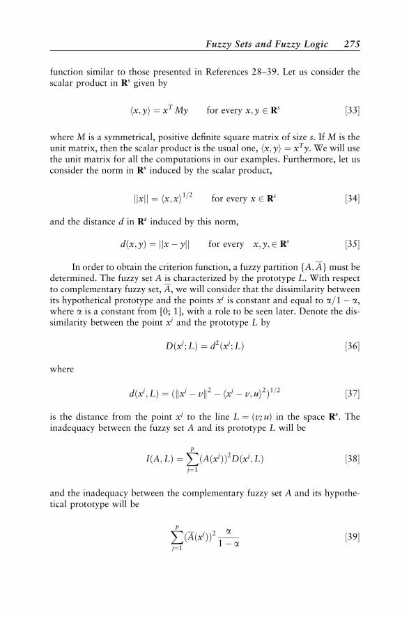
function similar to those presented in References 28–39. Let us consider thescalar product in Rs given by

hx; yi ¼ xT My for every x; y 2 Rs ½33�

where M is a symmetrical, positive definite square matrix of size s. If M is theunit matrix, then the scalar product is the usual one, hx; yi ¼ xTy. We will usethe unit matrix for all the computations in our examples. Furthermore, let usconsider the norm in Rs induced by the scalar product,

jjxjj ¼ hx;xi1=2 for every x 2 Rs ½34�

and the distance d in Rs induced by this norm,

dðx; yÞ ¼ jjx � yjj for every x; y;2 Rs ½35�

In order to obtain the criterion function, a fuzzy partition fA;Ag must bedetermined. The fuzzy set A is characterized by the prototype L. With respectto complementary fuzzy set, A, we will consider that the dissimilarity betweenits hypothetical prototype and the points xj is constant and equal to a=1 � a,where a is a constant from [0; 1], with a role to be seen later. Denote the dis-similarity between the point xj and the prototype L by

Dðxj;LÞ ¼ d2ðxj;LÞ ½36�

where

dðxj;LÞ ¼ ðkxj � vk2 � hxj � v; ui2Þ1=2 ½37�

is the distance from the point xj to the line L ¼ ðv; u) in the space Rs. Theinadequacy between the fuzzy set A and its prototype L will be

IðA;LÞ ¼Xp

j¼1

ðAðxjÞÞ2Dðxj;LÞ ½38�

and the inadequacy between the complementary fuzzy set A and its hypothe-tical prototype will be

Xp

j¼1

ðAðxjÞÞ2 a1 � a

½39�


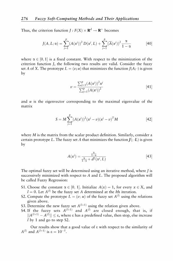
Thus, the criterion function J : FðXÞ � Rd ! Rþ becomes

JðA;L; aÞ ¼Xp

j¼1

ðAðxjÞÞ2 Dðxj;LÞ þXp

j¼1

ðAðxjÞÞ2 a1 � a

½40�

where a 2 ½0; 1� is a fixed constant. With respect to the minimization of thecriterion function J, the following two results are valid. Consider the fuzzyset A of X. The prototype L ¼ ðv; uÞ that minimizes the function J(A; �) is givenby

v ¼Pp

j¼1ðAðxjÞÞ2xjPpj¼1ðAðxjÞÞ2

½41�

and u is the eigenvector corresponding to the maximal eigenvalue of thematrix

S ¼ MXp

j¼1

ðAðxjÞÞ2ðxj � vÞðxj � vÞTM ½42�

where M is the matrix from the scalar product definition. Similarly, consider acertain prototype L. The fuzzy set A that minimizes the function Jð; �LÞ is givenby

AðxjÞ ¼a

1�aa

1�a þ d2ðxj;LÞ ½43�

The optimal fuzzy set will be determined using an iterative method, where J issuccessively minimized with respect to A and L. The proposed algorithm willbe called Fuzzy Regression:

S1. Choose the constant a 2 ½0; 1�. Initialize AðxÞ ¼ 1, for every x 2 X, andl ¼ 0. Let AðlÞ be the fuzzy set A determined at the lth iteration.

S2. Compute the prototype L ¼ ðv; uÞ of the fuzzy set AðlÞ using the relationsgiven above.

S3. Determine the new fuzzy set Aðlþ1Þ using the relation given above.S4. If the fuzzy sets Aðlþ1Þ and AðlÞ are closed enough, that is, if

jjAðlþ1Þ � AðlÞjj � e, where e has a predefined value, then stop, else increasel by 1 and go to step S2.

Our results show that a good value of e with respect to the similarity ofAðlÞ and Aðlþ1Þ is e ¼ 10�5.


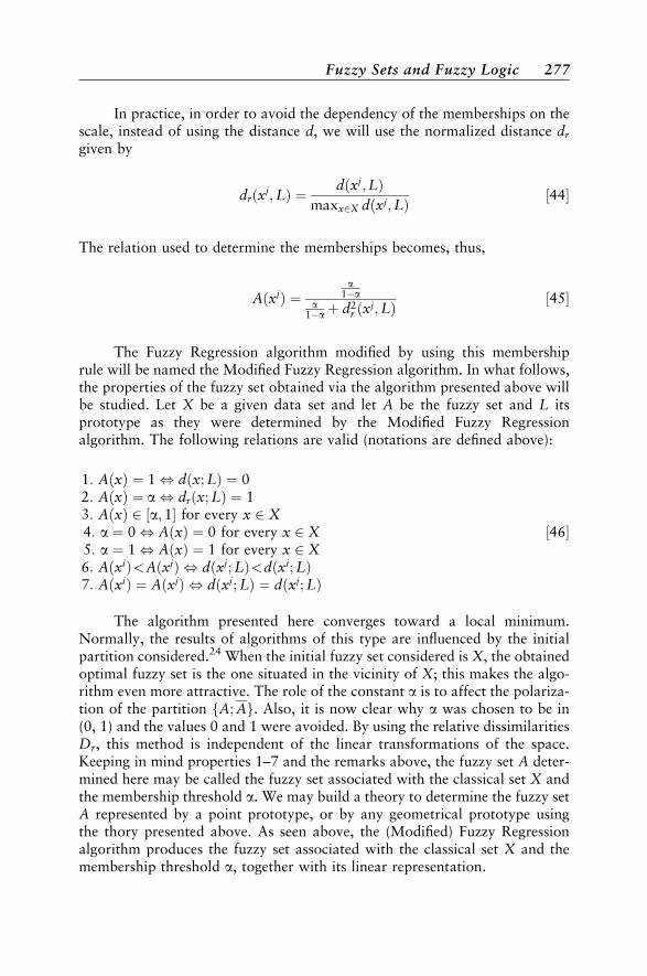
In practice, in order to avoid the dependency of the memberships on thescale, instead of using the distance d, we will use the normalized distance dr

given by

drðxj;LÞ ¼ dðxj;LÞmaxx2X dðxj;LÞ ½44�

The relation used to determine the memberships becomes, thus,

AðxjÞ ¼a

1�aa

1�a þ d2r ðxj;LÞ ½45�

The Fuzzy Regression algorithm modified by using this membershiprule will be named the Modified Fuzzy Regression algorithm. In what follows,the properties of the fuzzy set obtained via the algorithm presented above willbe studied. Let X be a given data set and let A be the fuzzy set and L itsprototype as they were determined by the Modified Fuzzy Regressionalgorithm. The following relations are valid (notations are defined above):

1: AðxÞ ¼ 1 , dðx;LÞ ¼ 02: AðxÞ ¼ a , drðx;LÞ ¼ 13: AðxÞ 2 ½a; 1� for every x 2 X4: a ¼ 0 , AðxÞ ¼ 0 for every x 2 X5: a ¼ 1 , AðxÞ ¼ 1 for every x 2 X6: AðxiÞ<AðxjÞ , dðxj;LÞ<dðxi;LÞ7: AðxiÞ ¼ AðxjÞ , dðxj;LÞ ¼ dðxj;LÞ

½46�

The algorithm presented here converges toward a local minimum.Normally, the results of algorithms of this type are influenced by the initialpartition considered.24 When the initial fuzzy set considered is X, the obtainedoptimal fuzzy set is the one situated in the vicinity of X; this makes the algo-rithm even more attractive. The role of the constant a is to affect the polariza-tion of the partition fA;Ag. Also, it is now clear why a was chosen to be in(0, 1) and the values 0 and 1 were avoided. By using the relative dissimilaritiesDr, this method is independent of the linear transformations of the space.Keeping in mind properties 1–7 and the remarks above, the fuzzy set A deter-mined here may be called the fuzzy set associated with the classical set X andthe membership threshold a. We may build a theory to determine the fuzzy setA represented by a point prototype, or by any geometrical prototype usingthe thory presented above. As seen above, the (Modified) Fuzzy Regressionalgorithm produces the fuzzy set associated with the classical set X and themembership threshold a, together with its linear representation.


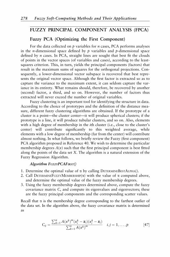
FUZZY PRINCIPAL COMPONENT ANALYSIS (FPCA)

Fuzzy PCA (Optimizing the First Component)

For the data collected on p variables for n cases, PCA performs analysesin the n-dimensional space defined by p variables and p-dimensional spacedefined by n cases. In PCA, straight lines are sought that best fit the cloudsof points in the vector spaces (of variables and cases), according to the least-squares criterion. This, in turn, yields the principal components (factors) thatresult in the maximum sums of squares for the orthogonal projections. Con-sequently, a lower-dimensional vector subspace is recovered that best repre-sents the original vector space. Although the first factor is extracted so as tocapture the variance to the maximum extent, it can seldom capture the var-iance in its entirety. What remains should, therefore, be recovered by another(second) factor, a third, and so on. However, the number of factors thusextracted will never exceed the number of original variables.

Fuzzy clustering is an important tool for identifying the structure in data.According to the choice of prototypes and the definition of the distance mea-sure, different fuzzy clustering algorithms are obtained. If the prototype of acluster is a point—the cluster center—it will produce spherical clusters; if theprototype is a line, it will produce tubular clusters, and so on. Also, elementswith a high degree of membership in the ith cluster (i.e., close to the cluster’scenter) will contribute significantly to this weighted average, whileelements with a low degree of membership (far from the center) will contributealmost nothing. In what follows, we briefly review the Fuzzy (first component)PCA algorithm proposed in Reference 40. We wish to determine the particularmembership degrees A(x) such that the first principal component is best fittedalong the points of the data set X. The algorithm is a natural extension of theFuzzy Regression Algorithm.

Algorithm FUZZYPCAFIRST()

1. Determine the optimal value of a by calling DETERMINEBESTALPHA().2. Call DETERMINEFUZZYMEMBERSHIP(a) with the value of a computed above,

and determine the optimal value of the fuzzy membership degrees.3. Using the fuzzy membership degrees determined above, compute the fuzzy

covariance matrix C, and compute its eigenvalues and eigenvectors; theseare the fuzzy principal components and the corresponding scatter values.

Recall that a is the membership degree corresponding to the farthest outlier ofthe data set. In the algorithm above, the fuzzy covariance matrix is determinedas

Cij ¼Pn

k¼1 AðxkÞmðxki � �xxiÞðxk

j � �xxjÞPnk¼1 AðxkÞm i; j ¼ 1; . . . ; p ½47�


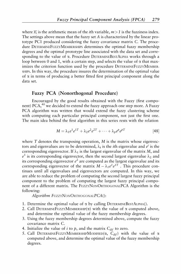
where xi is the arithmetic mean of the ith variable, m>1 is the fuzziness index.The settings above mean that the fuzzy set A is characterized by the linear pro-totype PC1 produced considering the fuzzy covariance matrix C. The proce-dure DETERMINEFUZZYMEMBERSHIPS determines the optimal fuzzy membershipdegrees and the optimal prototype line associated with the data set and corre-sponding to the value of a. Procedure DETERMINEBESTALPHA works through aloop between 0 and 1, with a certain step, and selects the value of a that max-imizes the criterion function used by the procedure DETERMINEFUZZYMEMBER-

SHIPS. In this way, the procedure insures the determination of the optimal valueof a in terms of producing a better fitted first principal component along thedata set.

Fuzzy PCA (Nonorthogonal Procedure)

Encouraged by the good results obtained with the Fuzzy (first compo-nent) PCA,40 we decided to extend the fuzzy approach one step more. A FuzzyPCA algorithm was written that would extend the fuzzy clustering schemewith computing each particular principal component, not just the first one.The main idea behind the first algorithm in this series rests with the relation

M ¼ l1e1e1T þ l2e2e2T þ � � � þ lpepepT ½48�

where T denotes the transposing operation, M is the matrix whose eigenvec-tors and eigenvalues are to be determined, li is the ith eigenvalue and ei is thecorresponding eigenvector. If l1 is the largest eigenvalue of the matrix M, ande1 is its corresponding eigenvector, then the second largest eigenvalue l2 andits corresponding eigenvector e2 are computed as the largest eigenvalue and itscorresponding eigenvector of the matrix M � l1e1e1T . This procedure con-tinues until all eigenvalues and eigenvectors are computed. In this way, weare able to reduce the problem of computing the second largest fuzzy principalcomponent to the problem of computing the largest fuzzy principal compo-nent of a different matrix. The FUZZYNONORTHOGONALPCA Algorithm is thefollowing:

Algorithm FUZZYNONORTHOGONALPCA():

1. Determine the optimal value of a by calling DETERMINEBESTALPHA().2. Call DETERMINEFUZZYMEMBERSHIP(a) with the value of a computed above,


covariance matrix C.4. Initialize the value of i to p, and the matrix Cdif to zero.5. Call DETERMINEFUZZYMEMBERSHIPMODIFIED(a, Cdif ) with the value of a

computed above, and determine the optimal value of the fuzzy membershipdegrees.

Fuzzy Principal Component Analysis (FPCA) 279

6. Using the fuzzy membership degrees determined above, compute the fuzzycovariance matrix C.

7. Compute the eigenvalues and eigenvectors of matrix C; the largesteigenvalue, and its corresponding eigenvector e are the ith largest fuzzyprincipal component and its corresponding scatter value.

8. Update the matrix Cdif by adding the value leeT using the eigenvalue andeigenvector from the preceding step.

9. Decrease the value of i by 1. If i>0, go to Step 5 and continue from there.Otherwise, stop the algorithm.

The procedure DETERMINEFUZZYMEMBERSHIPMODIFIED(a, Cdif ) is a modi-fied version of DETERMINEFUZZYMEMBERSHIPS, and determines the optimal fuzzymembership degrees and the optimal prototype line associated with the dataset and corresponding to the value of a and with the diminishing matrixCdif . The quantity in Cdif is the exact quantity that should be subtractedfrom the original covariance matrix C in order to determine the subsequenteigenvector and eigenvalue. But, because in this case the fuzzy covariancematrix depends on fuzzy membership degrees corresponding to a differentfuzzy set for each principal component, this subtraction will have to berepeated each time during the process of determining the line prototypes.

Fuzzy PCA (Orthogonal)

The main issue with the Fuzzy PCA algorithm described in the precedingsection is that the computed eigenvectors, while being unit vectors, are notmutually orthogonal. The next algorithm is designed to change this. Let usdenote l1; . . . ; lp, and e1; . . . ; ep the eigenvalues and the eigenvectors, respec-tively, that will finally be produced by our suggested algorithm. The first fuzzyprincipal component is computed as with the FUZZYPCAFIRST algorithm, thatis, by finding the optimal fuzzy membership degrees and the optimal linearprototype for the data set. Let us denote l01; . . . ; l

0p and e01; . . . ; e

0p the eigenva-lues and eigenvectors, respectively, produced in this way. Therefore, we willhave

l1 ¼ l01 ½49a�

and

e1 ¼ e01 ½49b�

The major novelty of this algorithm is in the way the other fuzzy principalcomponents are computed. The original data set is projected onto the hyper-plane orthogonal to the first fuzzy principal component, that is, determined byall the other principal components, as determined by the Fuzzy First Compo-nent PCA algorithm. Practically, this may be done by computing the scores


and removing the first item from the data vectors. Therefore, we first computethe scores:

x0jT ¼ xjT � ðe01; . . . ; e0pÞ ½50�

and then remove the first component of x0j, thus producing a subset X0of Rp�1:

X0 ¼ fðx02; . . . ; x

0pj9j : x0j ¼ ðx01; x02; . . . ; x0pÞg ½51�

This produces a data set in a Euclidean space of dimension p�1, where p is thesize of the original data set. Denote l001; . . . ; l

00p�1 and e001; . . . ; e00p�1 the eigen-

values and eigenvectors, respectively, produced in this way. The firstfuzzy principal component of this projected data set, after being rewritten interms of the original space, is orthogonal on the first fuzzy principal compo-nent, as computed originally. In order to account for the fuzziness in the fuzzydata sets, when rewriting the components in terms of the original space, theeigenvalues computed in the p�1 sized space will be multiplied by the fuzzyset fuzziness index fA, given by

fA ¼ 1

n

Xn

i¼1

AðxjÞm ½52�

Thus

l2 ¼ l001 � fA ½53�

and

e2T ¼ ð0; e001ÞT � ðe01; . . . ; e0pÞT ½54�

where (0; e001) denotes a vector having 0 for the first component, and the com-ponents of the vector e001 for the other components. In order to determine thethird fuzzy principal component we will reason in the same way, but here westart with the projected data set and project it onto the hyperplane orthogonalto the first two fuzzy principal components. This twice-projected data set willbe in a Euclidean space of dimension p�2. Let us suppose that, after propertransformations have been made at the superior level, these newly producedeigenvectors and eigenvalues (now in the Rp � 1 space) and still denoted byl001; . . . ; l

00p�1 and by e001; . . . ; e00p�1. These notations will replace the already

computed values.Now we need only a final transformation: to revert these eigenvectors

and eigenvalues to the original space. We use relations similar to those usedfor computing the initial projection, but in reverse. The FUZZYORTHOGONAL-PCA Algorithm is the following:

Fuzzy Principal Component Analysis (FPCA) 281

Algorithm FUZZYORTHOGONALPCA():

1. If p � 2, call FUZZYPCAFIRST(), otherwise continue.2. Determine the optimal value of a by calling DETERMINEBESTALPHA().3. Call DETERMINEFUZZYMEMBERSHIP(a) with the value of a computed above,


covariance matrix C.5. Compute the eigenvalues and eigenvectors of matrix C; the largest

eigenvalue, and its corresponding eigenvector e are the current fuzzyprincipal component and its corresponding scatter value.

6. Compute the scores of the data set and remove the first component of eachdata item.

7. Recursively call FUZZYORTHOGONALPCA() on this reduced data set; afterreturning, the values l001; . . . ; l

00p�1 and the corresponding eigenvectors

e001; . . . ; e00p�1 will be known, but will be computed in the projected space.8. Revert to the original data space and rewrite the eigenvalues and their

corresponding eigenvectors in terms of the original data space.

FUZZY EXPERT SYSTEMS (FUZZY CONTROLLERS)

A Fuzzy Expert System is an expert system that uses a collection of fuzzymembership functions and fuzzy rules, instead of Boolean logic, to make deci-sions from data.41,42 The rules are of the form:

If x is low and y is high then z is medium ½55�

where x and y are input variables, z is an output variable and low, high, med-ium are called linguistic labels and have associated fuzzy membership func-tions. The antecedent of the rule describes to what extent the rule applies,and the conclusion of the rule assigns a membership function to each outputvariable. A Fuzzy Controller is a special type of fuzzy expert system whosepurpose is to influence the behavior of a system by changing its inputs accord-ing to a set of rules that describe how the system operates. The general infer-ence process proceeds in the following steps:

Linguistic LabelsAfter identifying the relevant input and output variables of the system,

and the range of their values, we need to select meaningful linguistic labelsfor each variable and associate them with appropriate fuzzy sets. The mostcommonly employed linguistic labels are approximately zero (AZ), positivesmall (PS), positive medium (PM), positive large (PL), negative small (NS),negative medium (NM), negative large (NL). The fuzzy sets associated with


these linguistic variables are generally fuzzy numbers, but, when needed,different fuzzy sets may be used.

Fuzzy Inference RulesThe knowledge to be used by the system is formulated in terms of fuzzy

inference rules. There are two distinct ways in which these fuzzy rules can bedetermined: (a) by using the experience of human operators; and (b) by obtain-ing them from empirical data found through suitable learning, for example,using neural networks. As stated before, the canonical form of the fuzzy infer-ence rules is

If e1 ¼ A and e2 ¼ B then v ¼ C ½56�

where A, B, and C are fuzzy membership functions associated with some of theavailable linguistic labels.

FuzzificationFor each fuzzy inference rule, the fuzzy sets associated with each input

variable are applied to their actual values, to determine the degree of truthfor each rule premise. The degree of truth for a rule premise, sometimesdenoted by a, is computed as a ¼ T1ðAðe1Þ, Bðe2ÞÞ, where T1 is a t-norm. Ifa for a certain rule is nonzero, then the rule is said to fire.

InferenceThe fuzzy set associated with the output variable is computed as

ruleðzÞ ¼ T2ða;CðzÞÞ ¼ T2ðT1ðAðe1Þ;Bðe2ÞÞ;CðzÞÞ ½57�

where T2 is a t-norm, not necessarily the same as T1. Two t-norms generallyused in this case are min and product.

CompositionAll the fuzzy sets associated by different rules to the same variable are

combined together to form a single fuzzy set for each output variable. Thisis realised by using a t-conorm, that is, by an abuse of notation,

fuzzyðzÞ ¼ Sðrule1ðzÞ; rule2ðzÞ; . . .Þ ½58�

where S is the chosen t-conorm. Two t-conorms generally used in this case aremax and sum. The latter is not really a t-conorm, and it produces fuzzy mem-berships >1. Thus, it may only be used when followed by an appropriatedefuzzification method.

Fuzzy Expert Systems (Fuzzy Controllers) 283

DefuzzificationSometimes, the fuzzy sets associated with the output variables offer suf-

ficient information, but often we need to provide a crisp value for each outputvariable given a set of values for the input variables. There are more defuzzi-fication methods that may be used here, and we stress that they are completelydifferent from the defuzzification methods used in fuzzy clustering.

* Center of gravity. The defuzzified value of a fuzzy set C is its fuzzycentroid.

* First of maxima. The defuzzified value of a fuzzy set C is its smallestelement having the highest membership degree.

* Middle of maxima. The defuzzified value of a fuzzy set C is the mean ofall elements having the highest membership degree.

* Max criterion. The defuzzified value of a fuzzy set C is an arbitraryelement having the highest membership degree.

* Height defuzzification. The elements with membership degrees lowerthan a certain threshold are completely discarded, and the Center-of-gravity method is applied to the remainder of the fuzzy set.

HYBRID SYSTEMS

The component techniques of soft computing are not competitive, butcomplementary. Much research has been done to study the ways this comple-mentarity can be exploited. Each of the components has features to offer apotential partnership. Systems that have such a partnership are called ‘‘hybridsystems’’. Fuzzy logic uses the concept of computing with words, it deals withimprecision and information granularity and is an important tool for approx-imate reasoning. Neural networks learn and adapt. Genetic algorithms makeuse of a systemized random search and are an important tool for optimization.These three may be combined in different ways, as described below.

Combinations of Fuzzy Systems and Neural Networks

Many types of combinations between fuzzy systems and neural networkshave been proposed and studied. In what follows, we use the definitions andclassification proposed by Detlef Nauck, from the Department of ComputerScience, Technical University of Braunschweig, Germany.43–46 A ‘‘neuro-fuzzy’’ or ‘‘neural fuzzy’’ system is a combination of neural networks andfuzzy systems in such a way that neural networks are used to determine para-meters of fuzzy systems. The main intention of a neuro-fuzzy approach is tocreate or improve a fuzzy system by means of neural network methods. Thesystem should always be interpretable in terms of fuzzy if-then rules. A ‘‘fuzzy


neural network’’ is a neural network that uses fuzzy methods to learn faster orto perform better. The main intention is the improvement of the neuralnetwork.

Fuzzy Neural NetworksFuzzy methods are also used to enhance the learning capabilities or per-

formance of a neural network. This can be done by using fuzzy rules to changethe learning rate, or by creating a network that works with fuzzy inputs.

Concurrent Neuro-Fuzzy ModelsA neural network and a fuzzy system may work together on the same

task, but without influencing each other, that is, neither system is used todetermine parameters of the other. Usually, the neural network preprocessesthe inputs or postprocesses the outputs of the fuzzy system.

Cooperative Neuro-Fuzzy ModelsA neural network may also be used to determine the parameters of a fuz-

zy system. After the learning phase, the fuzzy systems work without the neuralnetwork. Cooperative models use the following approaches: (a) learn fuzzysets off-line; (b) learn fuzzy rules off-line; (c) learn fuzzy sets on-line; (d) learnrule weights.

Hybrid Neuro-Fuzzy ModelsA neural network and a fuzzy system may be combined into one homo-

genous architecture. The system may be interpreted as a special neural net-work with fuzzy parameters, or as a fuzzy system implemented in a paralleldistributed form.

Fuzzy Genetic Algorithms

There are a few approaches in which fuzzy set theory and evolutionaryalgorithms become highly interactive partners. They mostly concern the fol-lowing alternatives.47,48

Fuzzy Encoding and Fuzzy Set Operations in Genetic AlgoritmsThere are two different issues involved here. The first concerns the

encoding of each variable that comes as a part of the optimization problem,using fuzzy logic. Excepting the case of variable encoding using real numbers,encoding supposes the transformation of a numerical value into a certainstring of symbols, from a finite and small alphabet. Instead of using a smallnumber of symbols, we use fuzzy sets (linguistic labels) such as NL, NM,NS, Z (Zero), PS, PM, and PL, which can also be of a different granularity.Of course, any result obtained during the GA search needs to be decoded.The fuzzy decoding mechanism is related to the particular fuzzy encoding

Hybrid Systems 285

applied previously. The second issue concerns the use of fuzzy set operations(t-norms, t-conorms, averaging operators, and compensation operators) fordeveloping recombination operators. Also, fuzzy meta-rules are used in theselection of crossover and mutation rates, based on previous experience, andwith the help of a series of fuzzy if-then rules, for example, on the populationsize and the generation time. For example, if population is small and genera-tion is short, then the crossover rate is medium and the mutation rate is large.

Evolutionary Computing in Development of Fuzzy ModelsThe optimization abilities of genetic algorithms are used to develop the

best set of rules to be used by a fuzzy inference engine. Another approachrelates to fuzzy or hard clustering problems based on objective function mini-mization. These problems are regarded as GA search problems (i.e., the pro-blem needs to be specifically encoded and genetic operators have to bedevised), and the optimal fuzzy partition is determined by using a GA search.Moreover, such techniques may also be used in the pipeline, with the best par-tition prototypes produced by the GA search used as the initial configurationfor the fuzzy clustering procedure.

Neuro-Genetic Systems

The performance of neural networks (NN) can be enhanced by the use ofgenetic algorithms. There are two different approaches.49,50

Use of GA to Improve the Behavior of NNThis approach includes the use of GA in order to (a) generate the weights

of a neural network; (b) generate the architecture of a neural network; and(c) generate both the weights and architecture of a neural network.

Use of NN to Improve the Behavior of GAThis approach defines the evaluation function of the genetic algorithm as

a neural network. The genetic operators are used to train the parameters of theneural network. The evaluation function is the forward stage of the neural net-work, while the genetic parameters are improved in the back-propagationstage of the neural network.

FUZZY CHARACTERIZATION ANDCLASSIFICATION OF THE CHEMICALELEMENTS AND THEIR PROPERTIES

It may seem that the problem of classification of the chemical elementshas already been solved by the development of the periodic table of elements


and that the single item remaining to be solved is to find a certain,adequate and suggestive as possible graphic representation.51–55 In fact, thegroups of the periodic table do not always explain the whole wealth ofrelations between the properties of the elements and of their compounds.Sometimes unexpected similarities exist between remote elements in the peri-odic system.

It is, of course, true that most properties of the elements are determinedby the outer-electron configurations of their atoms. These configurations are,of course, the basis for the arrangement of elements in the periodic table.However, this effect of the valence electrons is often quite indirect. Alongwith properties of single atoms, properties exist that are collectively deter-mined, for example, by the lattice structure.

Therefore, we may raise the problem of whether the classical structure ofthe periodic system is really fully concordant with all the physical and chemi-cal properties of the elements.32,33,53,54 In what follows, we try to repeat theearly procedure of Mendeleev, whose classification was not founded on elec-tron configuration but on observable data concerning physico-chemical prop-erties of the elements. The basic idea of our procedure is that the properties ofelements are gradual by nature. Therefore, we must acknowledge that theyshould be grouped in classes with no clearly cut boundaries. Hence, each ele-ment should belong mainly to a single class, but this does not mean that itcould not also belong with different small membership degrees to all the otherclasses.

If we admit that the membership degrees to a group have a gradual char-acter, we may obtain a more accurate classification of the elements, able toaccount for some irregularities of the standard classification. It also could sug-gest the occurrence of some new relationships between the elements.

This classification must use primary physical and chemical properties ofthe elements. Their selection is rather difficult since they have to be expressednumerically and have to be known for all the investigated elements. The methodapplied for the classification uses fuzzy set theory in order to obtain a cluster-ing of the set of chemical elements. This method is hierarchical and does notsuppose a preliminary knowledge with respect to the number of classes in thedata set, nor does it suppose a certain structure for the classes. Both the num-ber of classes and their mutual relationships will be detected by the classifica-tion algorithm used.

In order to identify which properties (variables) are responsible for theobserved similarities and dissimilarities between the chemical elements, wealso applied a very interesting algorithm, namely, fuzzy hierarchical cross-classification (FHiCC). The technique produces not only a fuzzy partitioningof the chemical elements but also a fuzzy partitioning of the physical and che-mical properties considered. Moreover, the fuzzy hierarchical characteristicsclustering (FHiChC) and fuzzy horizontal characteristics clustering (FHoChC)procedures showed very high similarities between the chemical and structural

Fuzzy Characterization and Classification of Elements 287

properties of elements and also between the structural and some of the physi-cal properties.

HIERARCHICAL FUZZY CLASSIFICATION OFCHEMICAL ELEMENTS BASED ON TENPHYSICAL PROPERTIES

In order to use the methods presented above to classify the chemical ele-ments, the problem we are first faced with is to decide the characteristics thisclassification is built upon. We started with 10 physical properties: relativeatomic mass, A (1), density, r (2), melting point, Tf (3), boiling point, Tb

(4), Pauling electronegativity, w (5), enthalpy of vaporization, DHv (6) andfusion, DHf (7), specific heat capacity, Cs (8), first ionization energy, Ei (9),and covalent radius, r (10).

These values are known for 84 elements.The classification hierarchy produced by using the 10 physical properties

mentioned above without scaling (nonnormalization) of data is presented inFigure 4. The first partition separates, roughly speaking, the elements of themain groups of the periodic system (class 1) from those of the secondarygroups (class 2). To class 1 belong the metals of group 12 (IIB) (Zn, Cd,Hg) and also Ag; all these elements have the d subshell completed and arein this way analogous to those in the main groups. Also, class 1 includesfour lanthanides (Sm, Eu, Tm, Yb), all of which have the 5d subshell vacant.The 4f subshell is complete for Yb and half-complete (4f 7) for Eu, that is,these elements have relatively stable subshell configurations. The elementsTm and Sm have one electron fewer than these configurations (4f 13, 4f 6).On the other hand, class 2 also contains six elements of the main groups(Be, B, Al, C, Si, Ge). On the whole, the first class contains elements withlower densities and melting and boiling points (smaller fusion and vaporiza-tion enthalpies).

The next step for class 1 differentiates mainly between metals (class 1.1)and nonmetals (class 1.2), although the latter class includes the alkali metalsK, Rb, and Cs and the group 12 (IIB) metals Cd and Hg. The elements of class1.2 have lower densities, melting and boiling points and, as a rule, high ioniz-ation energies and electronegativities. The dominant features here are, how-ever, the melting and boiling points, and this accounts for the presence ofsome very electropositive (K, Rb, Cs) or heavy (Hg) elements. However, themetals of this class (1.2), together with the solid nonmetals at room tempera-ture (P, S, Se, I), are separated as a class (1.2.1) from the typical gaseous non-metals at room temperature (class 1.2.2).

The last subdivision distinguishes a class (1.2.1.1) containing the alkalimetals (membership degrees—MDs—of � 0.60) and Se and Cd. The last onehas a smaller MD (0.43), only a little more than its MD for the class 1.1.2.


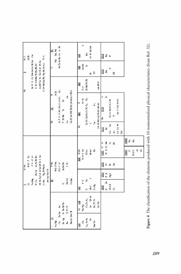
Fig

ure

4T

he

class

ifica

tion

of

the

elem

ents

pro

duce

dw

ith

10

nonnorm

ali

zed

physi

cal

chara

cter

isti

cs(f

rom

Ref

.32).

289

Class 1.1.2 includes, among others, Zn, which has a MD of 0.22 for the class1.2.1. The elements of the class 1.2.1.1 are similar mostly with respect to theirboiling points (� 700–750"C), while the elements of class 1.2.1.2 have lowerTb. Class 1.2.1.2 includes solid nonmetals (P, S, I) and Hg, elements with verysimilar ionization energies (240–250 kcal/mol). Nonmembers of this class, Asand Br, have MDs of 0.15–0.16 for it. It is interesting that grouped togetherhere are mercury and sulfur, elements that the alchemists thought to be at thesource of all matter.

From class 1.2.2 are first separated chlorine, bromine, and xenon (class1.2.2.1); among them, Cl and Br have similar MDs (0.79, 0.75), much higherthan Xe (0.59). The last is similar to them mostly with respect to its ionizationenergy. The other elements having much lower densities, Tf and Tb, aregrouped into two classes: one includes lighter noble gases, having the highestionization energies, He and Ne (1.2.2.2.2), the other contains the middle noblegases (Ar, Kr) along with hydrogen and the gaseous elements of period 2(N, O, F). These elements (class 1.2.2.2.1) have extremely low melting andboiling points and high ionization energies. To some extent, xenon alsobelongs to this class (MD of 0.25).

By dividing class 1.1, a quite large class (1.1.2) is obtained. This classcontains somewhat lighter elements, with lower boiling points (under1600"C): Li, Na [group 1 (IA)], all the elements of group 2 (IIA) of the periodictable (except beryllium), Tl from group 3 (IIIB), As, Sb, Bi from group 15(VA), Te [group 16 (VIA)], Zn [group 12(IIB)], and Eu and Yb (the lantha-nides with relatively stable configurations of the f -subshell, f 7 and f 14).From outside this class, some elements that have significant MDs for it areCd, Pb, Tm, Se, Rb, and Cs.

The other class (1.1.1) includes elements from group 13 (IIIA) (Ga, In),group 14 (IVA) (Sn, Pb), silver, and the lanthanides Sm and Tm. It is a ratherheterogeneous class, its elements having quite different properties and rela-tively small MDs, from 0.54 (Ga) to 0.26 (Tm). Also, related to this classare Ba, Bi, and Mn.

Now, passing to class 2, the lighter elements of the first and second seriesof transition metals (class 2.1) are separated from the heavier ones, with highermelting and boiling points (class 2.2). Class 2.1 contains, besides all the tran-sition metals of period 4, also most of those of period 5, lanthanum, and themajority of lanthanides, Th, U, and all the main group elements of class 2,except C. Class 2.2 includes transition metals of the period 5 and 6 as wellas carbon.

To continue, class 2.1 is separated from the set of elements with highboiling points (3300–4000"C) (class 2.1.2). From outside this class a few ele-ments have substantial MDs to it: La (0.42), Ce (0.38), B (0.29), Cr (0.27), Pt(0.26), Fe, Rh, and Pr (0.22 � � �0.24). The elements of class 2.1.1 are furthersubdivided into two classes that are rather less differentiated: the first one(class 2.1.1.1) contains Cu, Au, and La, and the early lanthanides (Ce, Pr,


Nd) as well as Al and Ge from the main group of the periodic table. The ele-ment Gd has a MD for this class (0.41) almost as high as to its own class(2.1.1.2): Be and Ag also have quite large MDs (nearly 0.20). Class 2.1.1.2contains Be, B, and Si, some transition metals of the first series, Y, and theheavier lanthanides. From outside this class, significant MDs occur for Cu,Ag, Al, Tm, and Sm.

From class 2.2 is separated a class (2.2.2) that includes the elements withthe highest Tf and Tb and very high densities (excepting carbon). The presenceof carbon together with molybdenum reminds us that molybdenite (MoS2)was considered for a long time to be graphite. The elements Pd and Th alsohave MDs for this class of � 0.15. The other class (2.2.1) is divided intotwo classes, their differences being again mainly the melting and boilingpoints; the more refractory metals (Ru, Hf, Ir) belong to the class 2.2.1.1(Mo and C also have MDs of � 0.15), while Rh and Pt form the class2.2.1.2 (Pd and Th have MDs for this class of � 0.14–0.16).

It is easy to notice that the criteria of melting and boiling points are thosethat dominate this classification. However, it appears that chemical propertiesare quite significant, as well.

In order to ensure a more uniform participation of various characteris-tics, we may use normalization (autoscaling) of the data. The classificationbased on the same 10 characteristics but normalized—a procedure that pre-vents certain properties, expressed by larger numerical values, to prevail–yields just four classes.

The final classification hierarchy including the membership degrees ofthe elements to the fuzzy sets of the final fuzzy partition is presented in Table 2.

The first separation is, as a matter of fact, the same as the one above.Only Be, Mn, and Al are moved into the class of main group elements, whileAg, Sm, and Tm are passed to the class of transition elements.

Thus, the separation of main group elements and transition metals ismore distinct here. Together with the main group elements are left Zn, Cd,and Hg (with complete d subshells), Mn (d5 configuration), and Eu and Yb(without electrons in the 5d subshell and stable configurations of the 4fsubshell). On the other hand, with the transition metals remain only C, Si,Ge, and B.

The elements from the main groups are divided next, as in the formerclassification, into metals (to which xenon joins also) and nonmetals, that is,again a more distinct separation than that without normalization. Finally, thetransition elements are divided into two classes: First, the more dense elementsfrom the period 5 (Nb–Pd) and 6 (Hf–Au), together with Th and U, as well asthe nonmetallic refractory elements from the main groups (B, C, Si); and,second, the early transition elements and the lanthanides, together with Ge.In this way, the classification is more like that given by chemical intuitionbut less detailed; we may say that by normalization a loss of informationarises.

Hierarchical Fuzzy Classification of Chemical Elements 291

Table 2 Membership Degrees to the Classes of the Final Partition Produced with10 Normalized Physical Properties

Element 1.1 1.2 2.1 2.2 Element 1.1 1.2 2.1 2.2

H 0.25 0.31 0.23 0.20 Tc 0.07 0.04 0.08 0.81He 0.26 0.37 0.22 0.16 Ru 0.12 0.07 0.08 0.73Li 0.40 0.32 0.19 0.09 Rh 0.09 0.05 0.05 0.80Be 0.30 0.30 0.25 0.16 Pd 0.08 0.04 0.26 0.61B 0.22 0.19 0.27 0.32 Ag 0.30 0.07 0.52 0.11C 0.20 0.18 0.22 0.40 Cd 0.65 0.19 0.12 0.03N 0.14 0.58 0.17 0.11 In 0.58 0.10 0.26 0.06O 0.16 0.54 0.18 0.13 Sn 0.52 0.09 0.32 0.06F 0.18 0.47 0.19 0.15 Sb 0.43 0.14 0.34 0.09Ne 0.25 0.40 0.21 0.14 Te 0.46 0.27 0.20 0.07Na 0.51 0.25 0.18 0.06 I 0.28 0.53 0.13 0.06Mg 0.57 0.27 0.12 0.04 Xe 0.40 0.32 0.20 0.09Al 0.46 0.20 0.25 0.09 Cs 0.40 0.19 0.29 0.12Si 0.24 0.20 0.28 0.29 Ba 0.44 0.11 0.35 0.09P 0.06 0.79 0.10 0.05 La 0.26 0.06 0.56 0.12S 0.08 0.74 0.12 0.06 Ce 0.28 0.07 0.54 0.12Cl 0.11 0.64 0.15 0.09 Pr 0.29 0.06 0.57 0.09Ar 0.29 0.42 0.19 0.10 Nd 0.29 0.05 0.59 0.07K 0.45 0.21 0.25 0.09 Sm 0.39 0.06 0.49 0.06Ca 0.54 0.14 0.25 0.07 Eu 0.44 0.09 0.39 0.08Sc 0.29 0.09 0.48 0.15 Gd 0.16 0.03 0.71 0.10Ti 0.18 0.07 0.48 0.27 Tb 0.14 0.03 0.74 0.09V 0.14 0.06 0.40 0.40 Dy 0.16 0.04 0.70 0.11Cr 0.21 0.09 0.47 0.24 Ho 0.14 0.03 0.71 0.12Mn 0.38 0.13 0.38 0.12 Er 0.13 0.03 0.69 0.14Fe 0.17 0.08 0.45 0.30 Tm 0.20 0.05 0.61 0.14Co 0.15 0.07 0.44 0.34 Yb 0.46 0.08 0.39 0.07Ni 0.15 0.07 0.44 0.34 Lu 0.10 0.03 0.55 0.31Cu 0.27 0.11 0.43 0.18 Hf 0.12 0.06 0.19 0.62Zn 0.58 0.38 0.04 0.01 Ta 0.15 0.09 0.17 0.59Ga 0.61 0.17 0.17 0.05 W 0.16 0.11 0.18 0.55Ge 0.22 0.13 0.36 0.29 Re 0.16 0.11 0.17 0.56As 0.32 0.31 0.24 0.13 Os 0.16 0.11 0.17 0.55Se 0.15 0.72 0.09 0.04 Ir 0.16 0.11 0.17 0.56Br 0.11 0.68 0.13 0.07 Pt 0.15 0.10 0.19 0.56Kr 0.33 0.39 0.18 0.09 Au 0.19 0.12 0.31 0.38Rb 0.44 0.19 0.27 0.10 Ag 0.37 0.27 0.25 0.12Sr 0.50 0.12 0.30 0.08 Tl 0.38 0.15 0.35 0.12Y 0.22 0.05 0.62 0.11 Pb 0.37 0.15 0.36 0.12Zr 0.10 0.04 0.51 0.35 Bi 0.37 0.15 0.36 0.12Nb 0.10 0.05 0.20 0.66 Th 0.14 0.06 0.36 0.44Mo 0.12 0.07 0.12 0.69 U 0.18 0.09 0.33 0.40


HIERARCHICAL FUZZY CLASSIFICATION OFCHEMICAL ELEMENTS BASED ON TEN PHYSICAL,CHEMICAL, AND STRUCTURAL PROPERTIES

In order to pass beyond the limits of this ‘‘physical’’ classification of ele-ments, we tried to base the classification on some chemical properties and fea-tures of electronic structure. We have thus kept only five physical propertiesdensity, r (1), melting point, Tf (2), boiling point, Tb (3), ionization energy,Ei (4), covalent radius, r (5), and, in exchange, five other chemical character-istics were added: two indices to describe the electron configuration, twoothers to describe the oxidation states, and the formation free energy for chlor-ides. For the characterization of electron configuration, and oxidation stateswe used values having the same number of digits. For the electron configura-tion, the first index, conf (6), is built as follows: The first digit gives the numberof electrons in the last (outermost) shell (1 � � �8), the next two digits give thenumber of electrons in the next to last shell (0 � � �18), and the final two decimaldigits give the number of electrons in the second to last shells (0 � � �32). Forexample, for chromium this index is 113.08. The second index, spdf (7), ofelectron configuration has as its first digit the number of electron shells inthe atom (1 � � �7), the next two digits give the number of d electrons in thenext to last shell (1 � � �10), and the two decimal digits give the number of felectrons in the second to last shell (1 � � �14). For example, for Cr this indexis 405.00 and for Gd is 601.07.

The index for positive oxidation states, osþ (8) contains the digits thatshow these states, in order of their importance, the most usual one being themost significant digit. Similarly, in order to describe the negative oxidationstates, os� (9), a negative number, was used, whose digits represent the oxi-dation states in decreasing order of their importance.

In order to characterize the chemical reactivity of an element, the forma-tion free energy (DFCl) of its chloride (10) was taken into account. The valueswere computed for the standard ambient temperature and pressure (298 K,1 bar) in kilocalories per mole of Cl.

The classification hierarchy produced by using the 10 properties dis-cussed above is shown in Figure 5.

It is interesting to see that the first separation into two classes is the sameas that for the classification based on the 10 physical properties: class 1 con-tains, as a whole, elements of the main groups of the periodic system and class2 elements of the secondary groups and most of the lanthanides. Silver is situa-ted just at the boundary of the two classes (membership degree, MD, of 0.50to class 1). The lanthanides with 4f 6 and 4f 13 configurations (Sm, Tm) alsohave small MDs for class 1 (0.63 and 0.57). Other elements having MDs of<0.7 for this class are Sn and Ga. On the other hand, the MD of Al for class2 is small (0.53). The element Mn also comes near class 1 (MD of 0.44), due to


Fig

ure

5T

he

class

ifica

tion

of

the

elem

ents

pro

duce

dw

ith

nonnorm

ali

zed

physi

cal,

chem

icaland

stru

ctura

lch

ara

cter

isti

cs(f

rom

Ref

.32).

294

its relatively stable electron configuration 4s23d.5 As an average, the elementsof class 1 have lower densities and clearly lower melting and boiling points,more electrons in the outermost shell (the elements in class 2 generally havetwo such electrons), an average of four shells, against five in class 2, lowerpositive oxidation states and a greater trend to negative oxidation states.The next division of class 1 is again mostly the same as for the 10 physicalproperties classification (class 1.1, metals; class 1.2, nonmetals plus K, Rb,Cs, and Hg). The single difference is the position of cadmium in class 1.1(with zinc) and not in the class 1.2 (with mercury).

The alkali metals as well as selenium lie near the boundary between theclasses. As an average, class 1.2 contains lighter elements having high ioniza-tion energies, more electrons in the last shell, a stronger trend toward negativeoxidation states, and a smaller affinity for chlorine. In class 1.1, but near theboundary of class 1.2, are situated As, Cd, and Na.

Class 1.2 is further divided in the same way as for the 10 physical proper-ties classification. Class 1.2.2 includes gaseous elements, with low densities,high ionization energies, smaller atomic radii, more electrons in the outermostshell, and weaker trends to positive oxidation states and to combininationwith chlorine. Chlorine itself is situated near the boundary of the class1.2.1. The MD for this class is mainly determined by the physical properties.Typical elements for this class are S and Se. The elements Cl, As, and Na alsohave significant MDs for this class.

While class 1.2.1 is not further divided here, class 1.2.2 is split up in adifferent manner than the classification based on physical properties: on theone hand, H, He, N, and Cl (1.2.2.1) and, on the other hand, the noble gasesfrom Ne to Xe, F, Br, and O (class 1.2.2.2). The former class generally con-tains lighter elements, with lower melting and boiling points (except for Cl,which is placed near the boundary of the class), with less electrons in the out-ermost shell and a marked trend for combinations of positive oxidation states(the elements in class 1.2.2.2 have almost no positive states). From class1.2.2.2, oxygen is the nearest to class 1.2.2.1. The separation between thetwo classes is not a clear one, except for the noble gases from Ne to Xe.

Class 1.1 is divided as for the 10 physical characteristics classification,with the difference that Ca, Sr, Ba, Bi, Eu, and Yb join with Ga, In, Sn, Pb,Ag, Sm, and Tm. Therefore, class 1.1.1 includes only main-group elementsand some elements of group 12 (IIB) (Zn, Cd). The elements Bi, Sb, and Srlie near the boundary of the two classes. Significant MDs for class 1.1.1 alsoexist for the other elements of group 1 (IA) (K, Rb) and group 2 (IIA) (Ca, Sr)as well as for As, Os, Se, Yb, Eu, In, Ga, and Sn. The elements Tl, Al, Mn, Li,Cu, As, Ge, and Mg belong to some extent to class 1.1.2.

Class 2 is also divided as in the previous classification. In class 2.2, thereactivity of the elements toward chlorine is a little below average. Among theelements of class 2, Pt and Rh are close to the boundary of class 2.1, while Nb,Pd, and Th of this latter class also have significant MDs for this class.


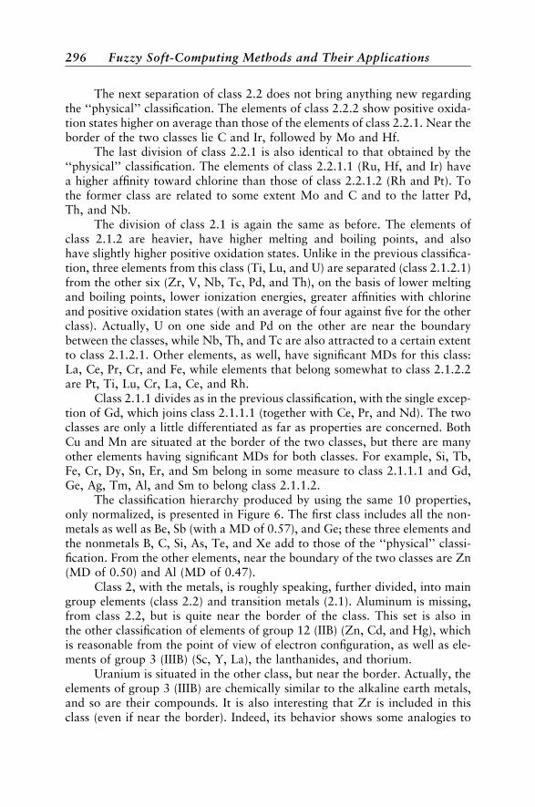
The next separation of class 2.2 does not bring anything new regardingthe ‘‘physical’’ classification. The elements of class 2.2.2 show positive oxida-tion states higher on average than those of the elements of class 2.2.1. Near theborder of the two classes lie C and Ir, followed by Mo and Hf.

The last division of class 2.2.1 is also identical to that obtained by the‘‘physical’’ classification. The elements of class 2.2.1.1 (Ru, Hf, and Ir) havea higher affinity toward chlorine than those of class 2.2.1.2 (Rh and Pt). Tothe former class are related to some extent Mo and C and to the latter Pd,Th, and Nb.

The division of class 2.1 is again the same as before. The elements ofclass 2.1.2 are heavier, have higher melting and boiling points, and alsohave slightly higher positive oxidation states. Unlike in the previous classifica-tion, three elements from this class (Ti, Lu, and U) are separated (class 2.1.2.1)from the other six (Zr, V, Nb, Tc, Pd, and Th), on the basis of lower meltingand boiling points, lower ionization energies, greater affinities with chlorineand positive oxidation states (with an average of four against five for the otherclass). Actually, U on one side and Pd on the other are near the boundarybetween the classes, while Nb, Th, and Tc are also attracted to a certain extentto class 2.1.2.1. Other elements, as well, have significant MDs for this class:La, Ce, Pr, Cr, and Fe, while elements that belong somewhat to class 2.1.2.2are Pt, Ti, Lu, Cr, La, Ce, and Rh.

Class 2.1.1 divides as in the previous classification, with the single excep-tion of Gd, which joins class 2.1.1.1 (together with Ce, Pr, and Nd). The twoclasses are only a little differentiated as far as properties are concerned. BothCu and Mn are situated at the border of the two classes, but there are manyother elements having significant MDs for both classes. For example, Si, Tb,Fe, Cr, Dy, Sn, Er, and Sm belong in some measure to class 2.1.1.1 and Gd,Ge, Ag, Tm, Al, and Sm to belong class 2.1.1.2.

The classification hierarchy produced by using the same 10 properties,only normalized, is presented in Figure 6. The first class includes all the non-metals as well as Be, Sb (with a MD of 0.57), and Ge; these three elements andthe nonmetals B, C, Si, As, Te, and Xe add to those of the ‘‘physical’’ classi-fication. From the other elements, near the boundary of the two classes are Zn(MD of 0.50) and Al (MD of 0.47).

Class 2, with the metals, is roughly speaking, further divided, into maingroup elements (class 2.2) and transition metals (2.1). Aluminum is missing,from class 2.2, but is quite near the border of the class. This set is also inthe other classification of elements of group 12 (IIB) (Zn, Cd, and Hg), whichis reasonable from the point of view of electron configuration, as well as ele-ments of group 3 (IIIB) (Sc, Y, La), the lanthanides, and thorium.

Uranium is situated in the other class, but near the border. Actually, theelements of group 3 (IIIB) are chemically similar to the alkaline earth metals,and so are their compounds. It is also interesting that Zr is included in thisclass (even if near the border). Indeed, its behavior shows some analogies to


those of the main group elements. The compound ZrO2 forms solid solutionswith CaO (used as a solid electrolyte), Zr shows some similarities to Be, and soon. The other d-block elements and U form the class 2.1. Consequently, theintroduction of chemical properties has little influence upon classification, astheir effect was indirectly contained within the physical properties taken intoaccount at the beginning.

FUZZY HIERARCHICAL CROSS-CLASSIFICATIONOF CHEMICAL ELEMENTS BASED ON TENPHYSICAL PROPERTIES

The classification hierarchy produced in this way for the 84 chemical ele-ments using characteristics (the 10 physical properties) without data normal-ization is presented in Figure 7. The first partitioning of elements in classes 1and 2 is exactly the same as in the analogous classification (Figure 4), and soare the partitioning of the second level, into classes 1.1, 1.2 and 2.1, 2.2. Whatis new is the partitioning of characteristics. Class 1 contains eight of the phy-sical properties, while class 2, which includes mostly elements in the secondarygroups of the periodic, table, is characterized mainly by the melting and boil-ing point. Their next division is into lighter transition metals (class 2.1) andheavier ones (class 2.2), and is associated with the separation by the meltingpoint, for the former class, and the boiling point, for the latter. There areno more subsequent divisions of the classes 2.1 and 2.2, while the analogousclassification above produced five clusters here.

The characteristic associated with class 1.1, comprised mostly of maingroup metals, is the ionization energy, but the boiling point and the atomicmass also have rather important MDs. Unlike the analogous classificationabove, the cross-clustering does not further divide this class, the only largerdivision being for class 1.2. Classes 1.2.1 and 1.2.2 are again the same as

Figure 6 The classification of the elements produced with normalized physical,chemical, and structural characteristics (from Ref. 32).

Fuzzy Hierarchical Cross-Classification 297

above. The elements of class 1.2.1, metals and nonmetals that are solid atroom temperature, have as their main characteristic the atomic mass, butthe boiling point also carries some weight. This class is not further divided,but neither are the typical gaseous nonmetals of the class 1.2.2. As inFigure 1, Cl, Br, and Xe are distinctly grouped (class 1.2.2.1), and their char-acteristic is the vaporization enthalpy, while from class 1.2.2.2 the lighter

1 H He

Li N O F Ne

Na Mg P S Cl Ar

K Ca Zn Ga As Se Br Kr

Rb Sr Ag Cd In Sn Sb Te I Xe

Cs Ba Hg Tl Pb Bi

Sm Eu Tm Yb

1 2 5 6 7 8 9 10

Be 2 B C

Al Si

Sc Ti V Cr Mn Fe Co Ni Cu Ge

Y Zr Nb Mo Tc Ru Rh Pd

La Hf Ta W Re Os Ir Pt Au

Ce Pr Nd Gd Tb Dy Ho Er Lu Th U

3 4

11

Li

Na Mg

Ca Zn Ga As

Sr Ag In Sn Sb Te

Ba Tl Pb Bi

Sm Eu Tm Yb

9

12

H He

N O F Ne

P S Cl Ar

K Se Br Kr

Rb Cd I Xe

Cs Hg

1 2 5 6 7 8 10

Be 21 B

Al Si

Sc Ti V Cr Mn Fe Co Ni Cu Ge

Y Zr Nb Tc Pd

La Au

Ce Pr Nd Gd Tb Dy Ho Er Lu Th U

3

22

C

Mo Ru Rh

Hf Ta W Re Os Ir Pt

4

121

P S

K Se

Rb Cd I

Cs Hg

1

122

H He

N O F Ne

Cl Ar

Br Kr

2 5 6 7 8 10

1221

Cl

Br

Xe

6

1222 H He

N O F Ne

Ar

Kr

2 5 7 8 10

12221 H

N O F

Ar

2 5 Kr

12222 He

Ne

7 8 10

122211

H

N O

2

122212

F

Ar

Kr

5

122221

He

7 8

122222

Ne

10

Figure 7 The classification of the elements and characteristics produced with 10nonnormalized physical properties (from Ref. 33).


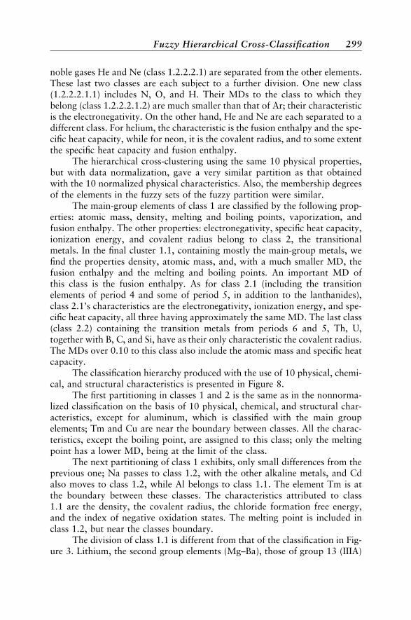
noble gases He and Ne (class 1.2.2.2.1) are separated from the other elements.These last two classes are each subject to a further division. One new class(1.2.2.2.1.1) includes N, O, and H. Their MDs to the class to which theybelong (class 1.2.2.2.1.2) are much smaller than that of Ar; their characteristicis the electronegativity. On the other hand, He and Ne are each separated to adifferent class. For helium, the characteristic is the fusion enthalpy and the spe-cific heat capacity, while for neon, it is the covalent radius, and to some extentthe specific heat capacity and fusion enthalpy.

The hierarchical cross-clustering using the same 10 physical properties,but with data normalization, gave a very similar partition as that obtainedwith the 10 normalized physical characteristics. Also, the membership degreesof the elements in the fuzzy sets of the fuzzy partition were similar.

The main-group elements of class 1 are classified by the following prop-erties: atomic mass, density, melting and boiling points, vaporization, andfusion enthalpy. The other properties: electronegativity, specific heat capacity,ionization energy, and covalent radius belong to class 2, the transitionalmetals. In the final cluster 1.1, containing mostly the main-group metals, wefind the properties density, atomic mass, and, with a much smaller MD, thefusion enthalpy and the melting and boiling points. An important MD ofthis class is the fusion enthalpy. As for class 2.1 (including the transitionelements of period 4 and some of period 5, in addition to the lanthanides),class 2.1’s characteristics are the electronegativity, ionization energy, and spe-cific heat capacity, all three having approximately the same MD. The last class(class 2.2) containing the transition metals from periods 6 and 5, Th, U,together with B, C, and Si, have as their only characteristic the covalent radius.The MDs over 0.10 to this class also include the atomic mass and specific heatcapacity.

The classification hierarchy produced with the use of 10 physical, chemi-cal, and structural characteristics is presented in Figure 8.

The first partitioning in classes 1 and 2 is the same as in the nonnorma-lized classification on the basis of 10 physical, chemical, and structural char-acteristics, except for aluminum, which is classified with the main groupelements; Tm and Cu are near the boundary between classes. All the charac-teristics, except the boiling point, are assigned to this class; only the meltingpoint has a lower MD, being at the limit of the class.

The next partitioning of class 1 exhibits, only small differences from theprevious one; Na passes to class 1.2, with the other alkaline metals, and Cdalso moves to class 1.2, while Al belongs to class 1.1. The element Tm is atthe boundary between these classes. The characteristics attributed to class1.1 are the density, the covalent radius, the chloride formation free energy,and the index of negative oxidation states. The melting point is included inclass 1.2, but near the classes boundary.

The division of class 1.1 is different from that of the classification in Fig-ure 3. Lithium, the second group elements (Mg–Ba), those of group 13 (IIIA)


Fig

ure

8T

he

class

ifica

tion

of

the

elem

ents

and

chara

cter

isti

cspro

duce

dw

ith

10

nonnorm

ali

zed

physi

cal,

chem

ical,

and

stru

ctura

lpro

per

ties

(fro

mR

ef.

33).

300

(Al–Tl), and Ag and Zn, are included in class 1.1.1, while in class 1.1.2 we findelements of groups 14 (IVA), 15 (VA), and 16 (VIA), together with the fourlanthanides (Sm, Eu, Tm, Yb). The separation is rather clear-cut. Elementswith significant MDs to class 1.1.1 include Cd, Cu, Na, Pb, and K and to class1.1.2 are Se, Mn, Ge, and Si. The characteristics of class 1.1.1 are the densityand covalent radius; smaller MDs are found for the ionization energy and thenegative oxidation states.

The chloride formation free energy and the index of negative oxidationstates belong to class 1.1.2. The division of class 1.2 is also different from theprevious: H, He, O, and F pass from class 1.2.2 to class 1.2.1, joining the alka-line metals (Na–Cs), Cd, and Hg, while in exchange P, S, Se, and I pass fromclass 1.2.1 to class 1.2.2, joining Cl, Br, and the noble gases Ne–Kr. Other ele-ments with important MDs to this last class are Hg, As, Cd, Te, and F. Thecharacteristic of this class is the electron configuration index for the outershell; another important MD is also obtained for the index for s, p, d, and fsubshells.

Class 1.2.1 is divided by the separation of the most electronegative ele-ments (O and F), forming class 1.2.1.1; Ne, Ar, and Hg also have significantMDs for this class. Their characteristics are the ionization energy and the num-ber of s, p, d, and f electrons in the outer shells, both with relatively smallMDs. Among the metals of class 1.2.1.1, Cd and Hg are at the border betweenthe two classes.

This class also has important MDs for Li and Zn. Here we find two char-acteristics: the index of positive oxidation states and the melting point (butwith a much smaller MD). Unlike the classification in Figure 6, class 2 isnot divided further; Tm, Sm, Al, Ag, Sn, and Sb are also related to this class.The characteristic here is the boiling point, but the melting point also has anMD of 0.49. In this case, the normalized cross-classification leads to a moreprofound division that is quite different from the previous ones. The classifica-tion hierarchy produced is represented in Figure 9. The first partitioning bringstogether in class 1 the main group elements: H, He; groups 1, 2, and 13 of theperiodic table (entirely); some elements of groups 14 (IVA)–17 (VIIA), and thenoble gases (except for Xe). Both Zn and Cd are joined, to these as usual, butalso Cu and Ag [group 11 (IB)] and Ni, as well as the three lanthanides (Sm,Eu, and Yb, i.e., without Tm) are also included. Their characteristics are den-sity, melting and boiling points, the s, p, d, and f configuration, and theoxidation states (positive and negative). Class 2 includes most of the d- andf -block elements, but also some p-block elements (from the groups 14(IVA)–18 (VIIIA)). Near the border of the two classes lie Co, Se, Y, and Tl.The characteristics here are ionization energy, covalent radius, the first indexof electron configuration, and the chloride formation free energy.

Furthermore, similar to other classifications, are the typical nonmetalsand noble gases He–Kr (class 1.2), which are separated from class 1, on theone hand, and the metals together with some refractory nonmetals (B, C, Si)


Fig

ure

9T

he

class

ifica

tion

of

the

elem

ents

and

chara

cter

isti

cspro

duce

dw

ith

10

norm

ali

zed

physi

cal,

chem

ical,

and

stru

ctura

lpro

per

ties

(fro

mR

ef.

33).

302

on the other hand, which are class 1.1. In class 1.1 the characteristics aredensity and positive oxidation states. From the partitioning of this latter classresults a class (class 1.1.2) that includes the alkaline metals (Li–Cs), the firstthree elements of groups 2 (IIA) and 13 (IIIA), Si, Ge, As, as well as Zn andCd; in other words, exclusively main-group elements and elements of group 12(IIB). Their characteristic is the positive oxidation state index. The other class(class 1.1.1) contains not only some elements of the main groups (Sr, Ba, In,Tl, and C) but also Sc, Ni, Cu, and Ag, and the three lanthanides, with densityas their characteristic. Other elements with significant MDs to class 1.1.1 areB, Co, Cs, Y, Fe, Cd, Ca, Ga, La, Ti, Pr, and Nd and to class 1.1.2 are C, Sr,Se, and S. The last four are main group elements.

The nonmetals, class 1.2, are more profoundly divided. Thus N, P, and Sare categorized separately (class 1.2.1) so that nitrogen is then classified aloneas a class (class 1.2.1.1), having the melting point as its characteristic. To theformer class, O and P are also related, with small MDs. For the latter class(class 1.2.1.1) of P and S (the only solid nonmetals among those of class1.2), some external elements with significant MDs are As, Br, Se, and S, andall solid nonmetals (except for the liquid bromine). Their characteristics arethe boiling point and the configuration index for s, p, d, and f electrons inthe outer shells. Class 1.2.2 contains gaseous nonmetals from groups 16(VIA)–18 (VIIIA) and also H and Br; smaller MDs to this class also exist forN, Li, Na, Si, and Xe. Here the characteristic that discriminates is the negativeoxidation state index.

All the p-block elements are grouped in class 2.1 from class 2 (from themain groups 14 (IVA)–18 (VIIIA)), the d-block elements of period 4 (Ti–Co),and some with lower melting and boiling points from the next periods as wellas the early lanthanides that are left (except for Lu). The properties includedhere are the energy of ionization and the first index of electronic configuration.The remaining class 2.2 elements are the heavy d-block elements of periods 5and 6: Nb–Rh and Hf–Au together with Lu, Th, and U. Lutetium lies, near theboundary between the two classes. Here the properties are the covalent radiusand the chloride formation free energy.

The elements of the main groups (except for Sn, which lies at the borderof the two classes) with Hg (class 2.1.1) and the transition metals (class 2.1.2)are separated from class 2.1. Elements from the outside with high MDs forclass 2.1.1 are Sn, Kr, and C and for class 2.1.2 are Ti, Ni, Lu, Pb, Sm, Hg,Eu, Ag, In, Nb, Yb, and Rh. The characteristics belonging there are the ioniza-tion energy (class 2.1.1) and the index of occupation of the outer electronicshell (class 2.1.2).

Class 2.2 is divided into two very distinct groups. The first one (class2.2.1) comprises Nb, Hf, Ta, Lu, Th, and U; related to them in some measureare several lanthanides (Er, Gd, Dy, Ho, Nd, Tm, Ce, and Pr) as well as V, Cr,and Zr. Their characteristic is the covalent radius. The heavy d-block elementsfrom periods 5 and 6: Mo to Rh and W to Au are included in class 2.2.2.


Elements with significant MDs to this class are Pd and Zr. The characteristic ofthis class is the chloride formation free energy.

It is interesting to remark that, by their form with successive ramifications,these classifications remind us of the ‘‘genealogical table’’ of elements proposedby Thierry William Preyer (1841–1897), who conceived a system, based on a genet-ical theory of elemental origin.55 However, the resemblance is purely formal.

FUZZY HIERARCHICAL CHARACTERISTICSCLUSTERING

In order to develop the classifications presented in this section, we willapply the fuzzy divisive hierarchical clustering (FDHiC) procedure describedin the theoretical section32,33 to different characteristic sets considered here.The hierarchical procedure obtained in this way is called fuzzy hierarchicalcharacteristics clustering (FHiChC).

The characteristics clustering with 10 physical properties for the 84elements gave essentially the same results as before, even if the succession ofthe splitting was changed a little. The membership degrees of the characteris-tics to the clusters of the final partition, with data normalization, are given inTable 3. To cluster 1, of atomic mass (A), the density (r) also has a significantmembership degree (MD ¼ 0.25). For the other properties and clusters, theMDs are near 1 and 0. A similar clustering procedure applied to the 10 phy-sical, structural, and chemical characteristics gave similar results. The classifi-cation hierarchy produced with nonnormalized data and the membershipdegrees of the characteristics to the clusters of the final fuzzy partition areshown in Table 4.

In the different steps of the clustering process the melting point (2),the boiling point (3), and the density (1) are successively separated. The twoother physical properties (ionization energy and covalent radius) and all the

Table 3 Membership Degrees of the 10 Physical Properties to theClusters of the Final Fuzzy Partition, with Data Normalization

Property 1 2.1 2.2.1 2.2.2

A (1) 0.99 0.00 0.00 0.00r (2) 0.25 0.75 0.00 0.00

Tf (3) 0.01 0.02 0.97 0.00Tb (4) 0.01 0.00 0.00 0.99w (5) 0.01 0.00 0.00 0.99DHv (6) 0.01 0.00 0.00 0.99DHf (7) 0.01 0.00 0.00 0.99Cs (8) 0.01 0.00 0.00 0.99Ei (9) 0.01 0.00 0.00 0.99r (10) 0.01 0.00 0.00 0.99


structural and chemical characteristics remain unsplit. Once again, with theexception of the density, only extreme MDs are obtained, The density is clas-sified with a MD of 0.22 to the class 1.1 of the boiling point.

The data normalization does not change the overall pattern of the clus-tering. The classification hierarchy differs only by the order of successiveseparations of the characteristics, the first now being the density (1), thenthe melting point (2), and the boiling point (3) and without any splitting forthe other seven characteristics to the final clusters. As is also apparent fromTable 4, most characteristics have values near unity and zero, except for themelting point, with an MD of 0.28 to the class 1 (of the density).

FUZZY HORIZONTAL CHARACTERISTICSCLUSTERING

In order to develop the classification presented in this section, we appliedthe well-known Fuzzy n-Means (FNM) algorithm.56 The classification proce-dure obtained in this way is called fuzzy horizontal characteristics clustering(FHoChC).

The characteristic clustering for the 10 physical properties, without datanormalization and with a predefined number of five classes, distribute thecharacteristics in three clusters only; the other two remain empty. Cluster 1contains the atomic mass (1), with an MD of 0.33; this characteristic appearswith equal MDs (0.33) to the two empty clusters, 3 and 4. In cluster 2, we findthe density (MD ¼ 1), while cluster 5 includes all the remaining eight physicalproperties, without any separation. All the MDs, except those for atomicmass, are either 1 or 0.

Let us remark that, even though five fuzzy classes were designed,the clustering actually produced only three: cluster 2, cluster 5, and another

Table 4 Membership Degrees of the 10 Physical, Chemical, and Structural Propertiesof the Clusters of the Final Fuzzy Partition, without and with Data Normalization

Without Data Normalization With Data Normalization

Property 1.1 1.2.1 1.2.2 2 1 2.1 2.2.1 2.2.2

r (1) 0.22 0.78 0.00 0.00 0.99 0.00 0.00 0.00Tf (2) 0.00 0.00 0.00 1.00 0.28 0.72 0.00 0.00Tb (3) 1.00 0.00 0.00 0.00 0.02 0.04 0.94 0.00Ei (4) 0.00 0.00 1.00 0.00 0.00 0.00 0.00 1.00r (5) 0.00 0.00 1.00 0.00 0.00 0.00 0.00 1.00conf (6) 0.00 0.00 1.00 0.00 0.00 0.00 0.00 1.00spdf (7) 0.00 0.00 1.00 0.00 0.00 0.00 0.00 1.00osþ (8) 0.00 0.00 1.00 0.00 0.00 0.00 0.00 1.00os� (9) 0.00 0.00 1.00 0.00 0.00 0.00 0.00 1.00DFCl (10) 0.00 0.00 1.00 0.00 0.00 0.00 0.00 1.00

Fuzzy Horizontal Characteristics Clustering 305

cluster that was equally divided into clusters 1, 3, and 4. These last three fuzzyclusters are identical, and they were produced simply because we asked for anumber of classes that correspond to the cluster substructure of the data setconsidered. In practical terms, we should consider only clusters 2 and 5 andthe union of clusters 1, 3, and 4. The same procedure, but with data normal-ization, produces only one empty class (class 5), with all the properties beingdistributed over four classes: In class 1 we find the atomic mass; in class 2 thedensity, and in class 3 the melting point, each of these properties having MDsequal to 1 for their own classes and 0 for the rest. Class 4 contains all the sevenother physical properties together, each of them with an MD ¼ 0.5; theseproperties also have MDs ¼ 0.5 for class 5, the vacant one.

The results are very much the same for the 10 physical, structural, andchemical characteristics, without data normalization. For the five predefinednumber of classes, one remains vacant; the MDs of all the characteristics forthis class are zero. From the other four classes, again three contain one char-acteristic each, while the last includes the rest of the seven properties. All theMDs are 1 or 0. The three properties separated are, again, the density (class 1),the melting point (class 2), and the boiling point (class 3).

The same treatment, but with a predefined number of four classes, givesthe same results, except for the missing empty class. This suggests another wayin which a number of classes higher than the natural number of classes thatcorresponds to the cluster substructure of the considered data set is found.In the preceding case, three fuzzy classes were absolutely identical, indicatingthat they were artificially split. In this case the clustering process actually pro-duced four fuzzy classes, the fifth one having MDs ¼ 0 for all the properties,being produced only to comply with the prerequisite of five classes that wasabove the natural number of four classes.

It is obvious from the discussions so far that on a chemical as well as aphysical basis the same partitions are almost invariably found. These essen-tially agree with the traditional chemical classifications, although the detailsmay differ. By using this approach, we retain the separation into main groupelements (s- and p-block elements), transition metals (d- and f -block ele-ments), and so on. Some elements may pass from one group to another,depending on the type of classification, but the general framework remainsunchanged from the traditional one. On the other hand, classification detailssuch as the membership degrees to various classes and the distances betweenelements point out some less trivial similarity relationships between the ele-ments. These might be suggestive of some new ideas with possible applicationsin different fields. Moreover, the fuzzy cross-classification procedure allowsfor qualitative and quantitative identification of the properties (physical, che-mical, and structural) responsible for observed similarities and dissimilaritiesbetween chemical elements. In addition, the fuzzy hierarchical characteristicsclustering (FHiChC) and fuzzy horizontal characteristics clustering (FHoChC)procedures revealed a high similarity between chemical and structural proper-


ties and also between the latter and some physical properties. The fact that thediscriminant and independent physical properties include relative mass, den-sity, and melting point illustrates that the results obtained in this way referespecially to the elementary substances and less to the elements as atom types.On the contrary, the classical periodic system of chemical elements considersfirst the properties (e.g., valence) of the chemical elements. Electronegativity,ionization energy, or covalent radius is mainly determined by electron config-uration. As a result they are grouped in the same cluster.

CHARACTERIZATION AND CLASSIFICATION OFLANTHANIDES AND THEIR PROPERTIESBY PCA AND FPCA

In the history of chemistry, one can hardly find a more intricate field thanthe discovery and classification of the rare earths elements. Their unusual simi-larity of properties, as well as their scarcity (which prevented the exact deter-mination of their properties) raised considerable difficulties. It is even probablethat the development of the periodic table would have been significantlydelayed were these elements already known in the middle of the nineteenthcentury. It has been affirmed57 that ‘‘the group of rare earths forms a littleperiodic system of their own, where all the relations of the main system arereproduced on a small scale’’.

After failing to classify the rare earths as homologues of other elements,the solution was to group the lanthanides together in a separate series.58 Theatomic model of Bohr made it possible to settle the number of lanthanides at14, but attempts to find relations within the group of rare earths never ceased.The chapter on lanthanides in van Spronsen’s book59 gives a rather historicallycomplete account, so only some of these relationships will be discussed here.

An early classification of the rare earths (the oxides of lanthanides) inrelation to their separation from ores, was in the ceritic earths (the oxidesfrom lanthanum to samarium) and yttric earths (from europium to lutetium,but also scandium and yttrium). A further refinement of analytical methodsmade it possible to split the yttric earths into terbic (europium, gadolinium,terbium), erbic (dysprosium, holmium, erbium, thulium), and ytterbic (ytter-bium and lutetium) earths, along with yttrium oxide and scandium oxide.

In the ‘‘arena’’ system of J. D. Clark,60 shown below, some of the lantha-nides are correlated with other groups of elements:

IIIb IVb Vb VIb VIIb Ia IIaY Zr Nb Mo Tc Rb SrLa Ce Pr Nd Pm Sm Eu Gd Tb Dy Ho Er Tm Yb

Lu

while seven lanthanides remain without analogues.

Characterization and Classification of Lanthanides 307

Scheele61 suggested that lanthanides could be classed, as could actinides,in new kinds of groups, c, as follows: Ic: thulium [as a homologue of rubidium(Ia) and silver (Ib)]; IIc: ytterbium; IIIc: lutetium; IVc: cerium, praseodymium,neodymium (as homologues of zirconium); Vc: promethium; VIc: samarium;VIIc: europium; VIIIc: gadolinium, terbium, dysprosium, holmium, erbium (ashomologues of ruthenium, rhodium, and palladium).

Ternstrom62 built upon this idea and divided lanthanides into two rowsafter gadolinium, and distributed them in c-groups as shown:

Sc

YLa Ce Pr Nd Pm Sm Eu Gd

Tb Dy Ho Er Tm Yb Lu

Group B3 C4 C5 C6 C2 C3

Another aspect, still under discussion, is the identity of the element thatshould be considered the homologue of yttrium in group 3. This role is usuallyassigned to lanthanum,with the seriesof lanthanidesgoing fromceriumto lutetium.However, there are also reasons to put lutetium in group 3, as the homologue ofyttrium, and thus begin the series of lanthanides with lanthanum.63

Since the problem of a rational classification for the rare earth elements,based on their properties, cannot be considered resolved, there would be a realchallenge to use the methods of multidimensional analysis to establish somecorrelations between these elements and group them in distinct classes, andat the same time find correlations among the properties used to characterizethem. We have applied PCA and Cluster Analysis to the study of 84 chemicalelements (including the lanthanides, except promethium), characterized by 10physical properties or 10 physical, chemical, and structural characteris-tics.52,53 The lanthanides cluster separately from other elements. Only euro-pium and ytterbium (the lanthanides with relatively stable electronicconfigurations, f 7 and f 14, respectively) appear as being close to the elementsof the main groups of the periodic table. Also, a certain analogy between theselanthanides and calcium and lead could be observed. Quite similar results werefound in a fuzzy classification of chemical elements.32,33 As a consequence,the processing and rational interpretation of the registered data concerningthe lanthanides appeared to be better performed using new chemometricmethods.6–12

Properties of Lanthanides Considered in This Study

We compared fuzzy principal component analysis (FPCA) to classicalPCA methods to characterize lanthanum, the 14 lanthanides, and the other


group 3 elements—scandium and yttrium, with the idea of clarifying the rela-tions of Sc and Y with the lanthanides. The characteristics selected as a basisfor the classification were almost exclusively physical properties. Propertieswere selected for which the values were known for all (or nearly all) the ele-ments under consideration. The data were taken from different tables or text-books.64,65 Since the values given in various sources often differ significantly,we tried to select the most probable values to make up a consistent data set. Aspecial case is that of promethium; data for this element are sometimes scarceand uncertain. For some properties, there are no reliable experimental data inthe literature, but the values are obtained by interpolation from those of theneighboring elements.

The 18 selected properties were atomic mass (A), density (d), atomicradius (r), first (I1), second (I2) and third (I3) ionization energy, Pauling elec-tronegativity (X), melting point (MP), boiling point (BP), enthalpy of fusion(HF), vaporization (HV), atomization (HA), standard entropy (S), specificheat capacity (SHC), surface tension (ST) at the melting point, electrical resis-tivity (ER), heat conductivity (HC), and the formation free energy of the chlor-ide LnCl3 per mol of Cl (FFE)—as a characteristic of chemical reactivity.

The electron configurations of the elements studied and of their triposi-tive ions are the following:

Sc (Z ¼ 21) [Ar] 3d14s2 Sc3þ [Ar]Y (Z ¼ 39) [Kr] 4d15s2 Y3þ [Kr]La (Z ¼ 57) [Xe] 5d16s2 La3þ [Xe]Ce (Z ¼ 58) [Xe] 4f 25d06s2 Ce3þ [Xe]4f 1

Pr (Z ¼ 59) [Xe] 4f 35d06s2 Pr3þ [Xe]4f 2

Nd (Z ¼ 60) [Xe] 4f 45d06s2 Nd3þ [Xe]4f 3

Pm (Z ¼ 61) [Xe] 4f 55d06s2 Pm3þ [Xe]4f 4

Sm (Z ¼ 62) [Xe] 4f 65d06s2 Sm3þ [Xe]4f 5

Eu (Z ¼ 63) [Xe] 4f 75d06s2 Ce3þ [Xe]4f 6

Gd (Z ¼ 64) [Xe] 4f 75d16s2 Gd3þ [Xe]4f 7

Tb (Z ¼ 65) [Xe] 4f 95d06s2 Tb3þ [Xe]4f 8

Dy (Z ¼ 66) [Xe] 4f 105d06s2 Dy3þ [Xe]4f 9

Ho (Z ¼ 67) [Xe] 4f 115d06s2 Ce3þ [Xe]4f 10

Er (Z ¼ 68) [Xe] 4f 125d06s2 Er3þ [Xe]4f 11

Tm (Z ¼ 69) [Xe] 4f 135d06s2 Tm3þ [Xe]4f 12

Yb (Z ¼ 70) [Xe] 4f 145d06s2 Yb3þ [Xe]4f 13

Lu (Z ¼ 71) [Xe] 4f 145d16s2 Lu3þ [Xe]4f 14

Therefore, Eu and Yb have relatively stable electron configurations; forthe ions, Gd3þ and Lu3þ should be the most stable, as well as Ce4þ , Tb4þ ,Eu2þ , Yb2þ . The elements La, Gd, and Lu have configurations analogous tothose of Sc and Y.


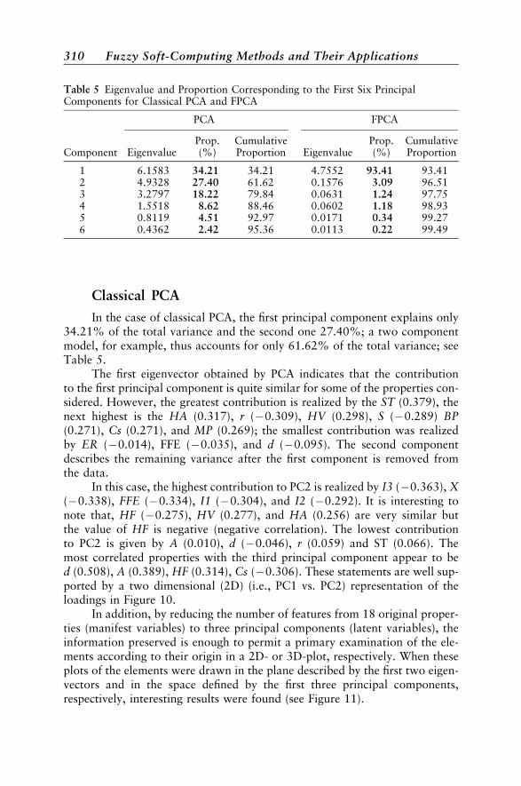
Classical PCA

In the case of classical PCA, the first principal component explains only34.21% of the total variance and the second one 27.40%; a two componentmodel, for example, thus accounts for only 61.62% of the total variance; seeTable 5.

The first eigenvector obtained by PCA indicates that the contributionto the first principal component is quite similar for some of the properties con-sidered. However, the greatest contribution is realized by the ST (0.379), thenext highest is the HA (0.317), r (�0.309), HV (0.298), S (�0.289) BP(0.271), Cs (0.271), and MP (0.269); the smallest contribution was realizedby ER (�0.014), FFE (�0.035), and d (�0.095). The second componentdescribes the remaining variance after the first component is removed fromthe data.

In this case, the highest contribution to PC2 is realized by I3 (�0.363), X(�0.338), FFE (�0.334), I1 (�0.304), and I2 (�0.292). It is interesting tonote that, HF (�0.275), HV (0.277), and HA (0.256) are very similar butthe value of HF is negative (negative correlation). The lowest contributionto PC2 is given by A (0.010), d (�0.046), r (0.059) and ST (0.066). Themost correlated properties with the third principal component appear to bed (0.508), A (0.389), HF (0.314), Cs (�0.306). These statements are well sup-ported by a two dimensional (2D) (i.e., PC1 vs. PC2) representation of theloadings in Figure 10.

In addition, by reducing the number of features from 18 original proper-ties (manifest variables) to three principal components (latent variables), theinformation preserved is enough to permit a primary examination of the ele-ments according to their origin in a 2D- or 3D-plot, respectively. When theseplots of the elements were drawn in the plane described by the first two eigen-vectors and in the space defined by the first three principal components,respectively, interesting results were found (see Figure 11).

Table 5 Eigenvalue and Proportion Corresponding to the First Six PrincipalComponents for Classical PCA and FPCA

PCA FPCA

Prop. Cumulative Prop. CumulativeComponent Eigenvalue (%) Proportion Eigenvalue (%) Proportion

1 6.1583 34.21 34.21 4.7552 93.41 93.412 4.9328 27.40 61.62 0.1576 3.09 96.513 3.2797 18.22 79.84 0.0631 1.24 97.754 1.5518 8.62 88.46 0.0602 1.18 98.935 0.8119 4.51 92.97 0.0171 0.34 99.276 0.4362 2.42 95.36 0.0113 0.22 99.49


Figure 10 PCA loadings plot for the 18 selected properties (PC1-PC2).

0.6

0.50.4

0.30.20.10.0

0.00.

10.20.

30.4

_0.1_0.2_0.3

_ 0.4 _

0.4_

0.3_

0.2_

0.10.0

0.10.2

0.30.4

0.5

_ 0.3_ 0.

2_ 0.1PC2

PC

3

PC1

SA

ERd

HVHABP

ST MPHF

I2

I1

I3

Cs

FFE

HC

r

X

Figure 11 PCA loadings plot for the 18 selected properties (PC1-PC2-PC3).


From the plot of the 17 elements on the plane described by PC1 and PC2(Figure 12), as well as in the space defined by the first three eigenvectors (Fig-ure 13), we see that the first separation groups together the ‘‘light’’ lanthanides(La, Ce, Pr, Nd, Pm, Sm, Eu) and Yb. In Figure 12, for example, they are situ-ated in the upper half of the diagram, with the elements from La to Eu placed

Figure 12 PCA scores plot for the lanthanides including La, Sc, and Y (PC1-PC2).

Yb

Eu

Sm

Pm

GdTb

Dy

Tm

HoEr

Lu

Sc

Na

Ce

PrLa

Y

43

2

1

0

-1

-2

-3

5

43

21

0-1

-2 -2

-4-6

-3-4

-5

4

2

0

6

8

PC2

PC

3

PC1

Figure 13 PCA scores plot for the lanthanides including La, Sc, and Y (PC1-PC2-PC3).


in the first quadrant and Yb in the second (Sm and Eu are on the boundary linebetween the quadrants). Ytterbium is added to the lighter lanthanides due toits similarity to europium. In the electron configurations of these elements, the4f level is less than one-half full, except for Eu (half-complete level, f 7) and Yb(complete level, f 14), the two elements with relatively stable configurations.The second group is that of the ‘‘heavier’’ lanthanides, situated in the lowerhalf of the graph (Figure 12), with Gd and Tb in the fourth quadrant andDy, Ho, Er, Tm in the third, together with Lu—placed at a higher distancefrom the other. The cluster of ‘‘light lanthanides’’ is further divided into onecluster including the first five elements (from La to Pm) and another containingthe elements with relatively stable electron configurations (Yb, Eu) and Sm,which has one electron fewer than such a configuration.

From the ‘‘heavier lanthanides’’, ‘‘the similarity chart’’ (2D plot) and‘‘the similarity space’’ (3D plot) differentiate the pair Gd–Tb from the clusterDy, Ho, Er, Tm, and from Lu.

The outlier position of lutetium among the lanthanides (unlike La, whichis much closer to its neighbors) assigns it as a homologue of Y in the thirdgroup of the periodic table. The other two outliers (Yb and Eu) are the ele-ments with relatively stable electron configuration and many of their proper-ties deviate from the regularities observed for the other lanthanides.

As a matter of fact, multidimensional and fuzzy analysis of the chemicalelements32,33 suggested some analogies of Eu and Yb with main group ele-ments. As for Lu and La, they have an electron configuration with one electronin the d subshell with the f subshell empty (La) or completely occupied (Lu),unlike the other lanthanides.

Fuzzy PCA

Results obtained from the same initial data set (17 elements and 18 prop-erties) using the fuzzy PCA algorithm described above are also shown inTable 5. The results obtained by applying FPCA are quite different from thePCA results. The first component explains 93.41% of the total variance andthe second one only 3.09%: A two component model thus accounts for96.51% of the total variance (as compared to 61.62% for PCA) and a threecomponent model accounts for 97.75% (as compared to 79.84% for PCA),for the fuzzy PCA method (see Table 5). Hence, the FPCA-derived componentsaccount for significantly more of the variance than their classical PCA counter-parts. The column corresponding to the first fuzzy eigenvector obtained in thiscase indicates that the contribution to the first component is also very differ-ent. The greatest contribution is realized by the HF (0.558), the next highest bythe MP (0.373), then I1 (0.360), X (0.339), and I2 (0.297). A less significantcontribution is obtained from the majority of the characteristics as is, forexample, HC (�0.039), S (0.046), ST (�0.055), and SHC (�0.051). Withrespect to the second principal component, the highest contribution in this


case is realized by the BP (�0.520), HC (0.415), HV (�0.412), HA (�0.389),I3 (0.294), and ER (�0.267). The third component appears to be well corre-lated with ER (0.730), HF (�0.354), HA (0.250). These statements are alsovery well confirmed by the 2D representation of loadings and 2D and 3Drepresentation of fuzzy factor scores, shown in Figures 14 and 15, and bettersupport the similarity between lanthanides and the correlations between theirproperties, respectively.

Examining all the pairs of variables for relationships between them, wefind, indeed, some rather strong correlations, as may also be the case for theircorrelation coefficients, r. Nevertheless, these relations should be consideredwith caution, particularly when generalizing to other elements. As a matterof fact, lanthanides are a rather peculiar group of elements; their propertiesare very similar, that is, the variation of a given property in the series of theseelements is rather limited and inferences to all the elements are doubtful. Keep-ing this in mind, we may, however, discuss the closest correlations (similari-ties) found here.

The highest correlation coefficient (0.98) is for enthalpy of vaporizationand standard enthalpy of atomization. For metals, the latter one is actually thestandard sublimation enthalpy and is given, according to Hess’ law, by thesum of the standard enthalpies of fusion and vaporization. The enthalpies ofvaporization are those at the boiling temperature and, therefore, lower thanthe standard ones. Other very close correlations are those between the boiling

Figure 14 FPCA loadings plot for the 18 selected properties (PC1-PC2).


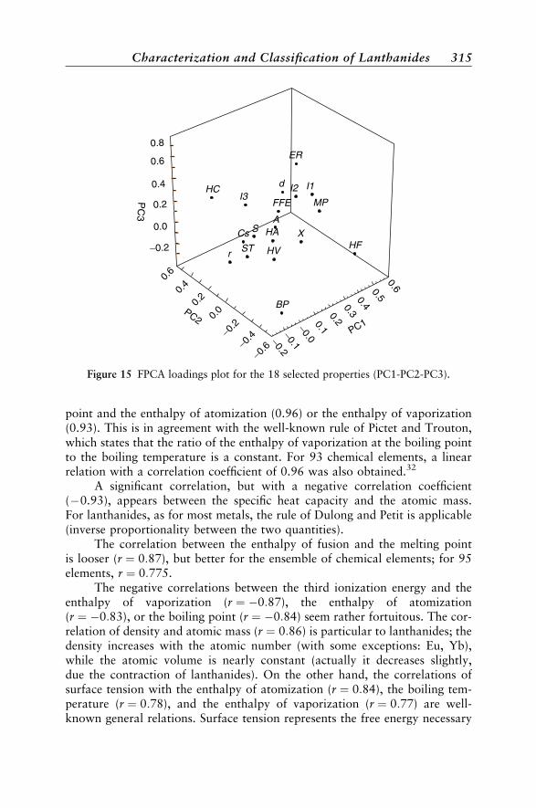
point and the enthalpy of atomization (0.96) or the enthalpy of vaporization(0.93). This is in agreement with the well-known rule of Pictet and Trouton,which states that the ratio of the enthalpy of vaporization at the boiling pointto the boiling temperature is a constant. For 93 chemical elements, a linearrelation with a correlation coefficient of 0.96 was also obtained.32

A significant correlation, but with a negative correlation coefficient(�0.93), appears between the specific heat capacity and the atomic mass.For lanthanides, as for most metals, the rule of Dulong and Petit is applicable(inverse proportionality between the two quantities).

The correlation between the enthalpy of fusion and the melting pointis looser (r ¼ 0:87), but better for the ensemble of chemical elements; for 95elements, r ¼ 0:775.

The negative correlations between the third ionization energy and theenthalpy of vaporization (r ¼ �0:87), the enthalpy of atomization(r ¼ �0:83), or the boiling point (r ¼ �0:84) seem rather fortuitous. The cor-relation of density and atomic mass (r ¼ 0:86) is particular to lanthanides; thedensity increases with the atomic number (with some exceptions: Eu, Yb),while the atomic volume is nearly constant (actually it decreases slightly,due the contraction of lanthanides). On the other hand, the correlations ofsurface tension with the enthalpy of atomization (r ¼ 0:84), the boiling tem-perature (r ¼ 0:78), and the enthalpy of vaporization (r ¼ 0:77) are well-known general relations. Surface tension represents the free energy necessary

0.8

0.6

0.4

0.2

0.2

0.4

0.6

0.0

_0.2

_ 0.4

_ 0.6

_ 0.2 _

0.0

_0.1

_0.2

0.10.2

0.30.4

0.50.6

0.0PC2

PC

3

PC1

SA

ER

d

HV

HA

BP

ST

MP

HF

I2 I1I3

Cs

FFEHC

r

X

Figure 15 FPCA loadings plot for the 18 selected properties (PC1-PC2-PC3).


for the creation of a new interface, and is therefore related to the energy spentin the splitting of bonds, the same entity that is implied in vaporization oratomization.

The variables selected as a basis for this classification were mainly phy-sical properties, with only the formation free energy of the chlorides as achemical property; no structural features, (electron configuration) or chemicalproperties (the oxidation state), were introduced. Nevertheless, the resultantclassification discriminates between groups of lanthanides with different struc-tural and chemical characters. Elements with oxidation state þ2 are groupedtogether, and so are elements with oxidation state þ4. Elements with similarpeculiarities of electron configuration are also put in the same cluster.

Based on this analysis and on the electron configuration, one may pro-pose a ‘‘periodic system’’ of the lanthanides (Figure 16). Setting lutetium asthe homologue of yttrium, the series of lanthanides begins with lanthanumand ends with ytterbium. It is broken into two rows, after europium, so thatelements with electron configurations up to f 7 are placed in the first row andthose with the f subshell more than half-full are in the second. There is alwaysa difference of 7 f -electrons between the homologous elements in the tworows. For this reason, these elements have the same number of additional elec-trons as compared with the relative stable configurations [Xe]6s2 (first row)and [Xe]4f 76s2 (second row) or the same number of electrons less than therelative stable configurations [Xe]4f 76s2 (first row) and [Xe]4f 146s2 (secondrow).

A broken line separates the two classes of ‘‘light’’ lanthanides, includingYb and the ‘‘heavier’’ lanthanides, together with Sc and Y. The clusters areframed by solid borders. Going along the series of lanthanides in the directionof the arrows we find all the clusters given by the fuzzy PCA analysis.

In comparison with the traditional splitting of the lanthanide series,59 themain difference is the placement of Gd in the second row. While the ions Gd3þ

and Lu3þ have the most stable configurations ([Xe]4f 7 and [Xe]4f 14, respec-tively). Among the neutral atoms, the most stable configurations are those ofEu; [Xe]4f 76s2 and Yb [Xe]4f 146s.2 Therefore, these two elements should playthe part of the ‘‘noble gases’’ in the system of lanthanides, and not Gd and Lu.

Figure 16 The ‘‘periodic system’’ of lanthanides.


On the other hand, the electron configuration of gadolinium [Xe]4f 75d16s2

makes this element the natural homologue of lanthanum [Xe]5d16s.2

Compared with the c-groups of Scheele,61 we find that his IVc-groupcontains the elements of the same cluster (Ce, Pr, Nd) and in his VIIIc-groupwe find the elements of two neighboring clusters: Gd and Tb, and Dy, Ho,and Er.

Obviously, the chemical intuition of the chemists who attempted to clas-sify the lanthanides led them to groupings similar in many respects to thosefound by the methods of multidimensional analysis.

Miscellaneous Applications of FPCA

Fuzzy Principal Component Analysis was also performed on the structuralfeatures concerned with the interaction of carbon–hydrogen bonds and molyb-denum–oxo bonds. In addition to all possible atom–atom distances and theangles subtended thereof, several additional metrics were defined and tabu-lated.66 These include the distance Rbp, and the angles a, b, and g, as wellas the dihedral MOCH, Scheme 1. Interactions between metal–oxo andcarbon–hydrogen bonds are of importance with respect to microbial andindustrial oxidation,67,68 and for these reasons molybdenum was the focusof this research.

Scheme 1

The results obtained from the initial dataset (71 complexes � 14 charac-teristics)—covariance matrix—were presented in Ref. 40. The results obtainedand the correlation data confirm that the structural features concerning inter-action of C–H and Mo––O bonds are related to each other and so could bereduced. Considering, for example, a two component model, FPCA accountsfor 97.20% of the total variance, and the first two PCA components account


for only 69.75%. It would take five-to-six classical principal components toaccount for the same total variance as two fuzzy principal components. Thelatter is, of course, much more desirable and makes for a significantly easierdataset analysis. Additionally, PCA showed only a partial separation of themolybdenum–oxo complexes onto the plane described by the first two princi-pal components, whereas a much sharper differentiation of the metric vari-ables along the diagonal is observed when FPCA is used.

FUZZY MODELING OF ENVIRONMENTAL,SAR AND QSAR DATA

Different fuzzy clustering algorithms mentioned above were successfullyapplied to the study of several German and Romanian natural mineral watersusing data obtained from samples collected from different sampling sites cov-ering, for example, a large percentage of the Romanian natural mineralwaters. The characteristic clustering technique produces fuzzy partitions ofthe mineral water properties involved and thus is a useful tool for studying(dis)similarities between different ions (i.e., speciation). The cross-classificationalgorithm provided not only a fuzzy partition of the mineral waters analyzed,but also a fuzzy partition of the characteristics considered. In this way, it ispossible to identify which ions and other physico-chemical features are respon-sible for the similarities or differences observed between different groups ofmineral waters.69

Various classification procedures—hierarchical and non-hierarchicalcrisp and fuzzy clustering, cross-classification fuzzy clustering, and PCA (var-imax rotation)—combined with receptor modeling were applied to a data setconsisting of wet deposition loads of major ions from five sampling sites inCentral Austria collected over a period of 10 years (1984–1993). The dataclassification with respect to the sampling sites as objects has shown that a distinctseparation between the northern Alpine rim and the inner Alpine region is achieved.This indicates the role of geographical disposition of the sampling sites.70

In a similar way, fuzzy cluster analysis and fuzzy recognition weresuccessfully used to model a large set of data from the Min River (China).71

The fuzzy analysis was employed as: A graphical tool to compare ecosystemswith respect to their pollution;72 to identify individual aerosol particles con-taining Cr, Pb, and Zn above the North Sea;73 at a rural site in Central Europeduring winter;74 to the characterisation of particulate matter from the KaraSea using electron probe X-ray micro analysis;75 to study the correlationbetween element concentrations in basal till and the uppermost layers ofmineral soil at forest sites in Finland76 or heavy metals in urban soil;77 tothe qualitative identification of trace elements in clinker;78 for the predictionof petrophysical rock parameters;79 to process on-line data streaming from fivemonitoring stations in Chile for forecasting SO2 levels;80 to data processing in


on-line laser mass spectrometry of inorganic, organic, or biological airborneparticles;81 and, finally, also for evaluation of PCDD/F emissions duringsolid-waste combustion.82

Fuzzy classification algorithms of the toxicity test systems based on thefirst 10 MEIC (international multicenter evaluation of in vitro cytotoxicitytests) chemicals allowed an objective interpretation of their similarities anddifferences. It was very interesting to observe the classification of toxicologicaltest systems on humans, considering their membership degrees. Some of themappeared closer to the test on rats and mice, and others seem to be very spe-cific. The Fuzzy Hierarchical Cross-Classification Algorithm (FHCsC) allowedthe qualitative and quantitative identification of the characteristics (chemicalcompounds) responsible for the observed similarities and dissimilaritiesbetween the toxicity test systems. In addition, the Fuzzy Hierarchical Charac-teristics Clustering (FHiCC) and Fuzzy Horizontal Characteristics Clustering(FHoCC) procedures revealed a high similarity between some MEIC chemicals(amitriptyline, digoxin, ethylene glycol, methanol, ethanol and isopropyl alco-hol) and a large difference among others (paracetamol, acetylsalicilic acid, fer-rous sulfate and diazepam). This result suggested the highly redundantcharacter of similar chemicals in the diagnosis of toxicological test systems.The results obtained clearly underline the efficiency of the fuzzy clusteringalgorithms for the comparison of different end points and the selection of abattery of in vitro toxicity tests that allow the estimation of the possible harm-ful effects of chemicals in vivo.83

Lack of certainty is a problem often found in ecological modeling, whichis a result of the large amount of variables to be considered. Consequently,many authors have suggested that applying fuzzy methods might be helpfulfor the interpretation of ecological data because the classification of chemicalsin terms of chemical groups or specific and baseline toxicity is rather vague. Inthe majority of papers dedicated to classifying existing chemicals accordingto their phytotoxicity84–86 and other ecotoxicological properties,87,88 thefuzzy clustering primary procedure used was based on the well-known Fuzzyc-Means algorithm.56

SPECTRAL LIBRARY SEARCH AND SPECTRAINTERPRETATION

It is becoming a common practice for modern instruments to be suppliedwith some form of data library of reference spectra that can be used to identifyunknown sample compounds. Most databases of this type consist of a list ofthe positions and intensities of the peaks contained within the spectra. Onceconversion of a sample spectrum has been carried out, its peak list can bematched against each entry in the library to find that which approximates itmost closely.

Spectral Library Search and Spectra Interpretation 319

Blaffert applied, for the first time, fuzzy sets for the identification of com-ponents in IR spectra of mixtures using peak positions and intensities.89 Themethod was implemented in a computer program that was capable of resol-ving multicomponent samples in infrared (IR) spectroscopy as well as X-raypowder diffractometry. The use of fuzzy set theory did not solve any problemscaused by experimental errors, but supports the integration of chemical andphysical knowledge into computerized interpretation of spectra in an illustra-tive manner.90 The algorithm described above, using IR spectra, has beenextended by considering the full spectral information, namely, peak position,intensity, and width.91–93

Spectroscopic and chromatographic methods are used to characterizemulticomponent samples with respect to chemical components and their con-centrations. Apart from the need to report accurate component concentra-tions, the analyses are frequently applied to ensure the quality of a finalproduct (e.g., by comparing the metal pattern of a steel sample with that ofa certified standard) or to classify a complex sample by means of its chroma-tographic profile used as a ‘‘fingerprint’’. The required data processingschemes are essentially methods of pattern recognition based on supervisedlearning techniques. However, the commonly used methods are not very suit-able for solving these kinds of problems because, at best, only a gross descrip-tion of the class shape is possible. To overcome these limitations Otto andBandemer, two of the most active chemists in the field of fuzzy set applicationsin analytical chemistry, have successfully applied fuzzy set theory to qualitycontrol of pharmaceutical products based on monitoring their ultraviolet(UV) spectra and for classifying samples by means of their chromatographicpatterns.94–97

The determination of double-bond positions in straight-chain alkenylcompounds is a provocative analytical problem when the amount of materialavailable is very small. In view of the frequent occurrence of functionalizedalkenes in the chemical structure of female sex pheromones of nocturnalmoths, rapid analytical procedures have been developed by fuzzy similarityanalysis of GC/MS and 13C NMR data.98,99 A more sophisticated methodol-ogy for protein 2D NMR assignment based upon protein spin coupling graphtheory analysis, fuzzy graph pattern recognition, and tree searching100 and a com-parison of depth profiles in SIMS by a fuzzy method101 has been also reported.

FUZZY CALIBRATION OF ANALYTICAL METHODSAND FUZZY ROBUST ESTIMATION OFLOCATION AND SPREAD

Quantitative determinations involving instrumentation are often ac-complished by establishing a calibration function. Calibration must be accom-plished before any measurements are made on a chemical system. Calibration


of an instrument for chemical quantification requires that the relationshipbetween the response of the instrument and the concentration be expressedmathematically. Several techniques for expressing this relationship areknown.27–29,101–106 The most common model is a linear regression, usuallya first-degree polynomial, although second- and high-degree polynomialshave been used.6–12

The ordinary linear least-squares regression is based on the assumptionof an independent and normal error distribution with uniform variance(homoscedastic). In addition, linear regression based on ordinary least-squarespresumes that errors in signal are much higher than those in concentration[error (Y) # error (X)]; it is also very sensitive to extreme data points, whichmay result in biased values of the regression parameters, slope, and intercept.

Some authors suggested that, in the absence of a good analytical model,the use of fuzzy regression could be one of the best approaches to the treat-ment of calibration data.107–111 The characteristics of performance of theFuzzy 1-Lines algorithm described above were very well illustrated in a com-parison study of a multitude of regression algorithms for analytical applica-tions,34–36 and also as a possibility of developing a fuzzy robust estimator ofmean (central location) and dispersion.112 Let us consider as an illustrativeexample the data discussed by Davies113 using a modified Huber algorithmto reduce the effect of outliers on central location. The data are presented inTable 6, and the computed results using eight different estimators of centrallocation are presented in Table 7. These are arithmetic mean, median, 5%trimmed mean, Huber (weighting constant 1.339), Hampel (weighting con-stants 1.700, 3.400, 8.500), Tukey (weighting constant 1.340), and Fuzzymean (a ¼ 0.1), respectively.

Case 1 refers to 50 normally distributed observations with a mean of10.00 and S. D. of 1. They were created using a pseudo-random number

Table 6 Relevant Data Sets Concerning Robust Methods Comparison Studies

Case 1: 9.08, 9.29, 9.32, 10.57, 10.72, 11.05, 10.36, 10.78, 10.33, 11.42, 10.43, 9.82,10.41, 10.93, 9.40, 8.94, 8.35, 9.14, 9.92, 8.66, 8.45, 10.35, 10.19, 9.47, 9.24,11.55, 11.12, 10.16, 9.43, 9.87, 10.63, 10.28, 11.34, 9.07, 9.43, 9.39, 9.68,11.98, 9.90, 10.08, 10.04, 9.67, 9.13, 8.92, 9.50, 9.71, 10.74, 11.13, 9.82,11.09

Case 2: 9.08, 9.29, 9.32, 10.57, 10.72, 11.05, 10.36, 10.78, 10.33, 11.42, 10.43, 9.82,10.41, 10.93, 9.40, 8.94, 8.35, 9.14, 9.92, 8.66, 8.45, 10.35, 10.19, 9.47, 9.24,11.55, 11.12, 10.16, 9.43, 9.87, 10.63, 10.28, 11.34, 9.07, 9.43, 9.39, 9.68,11.98, 9.90, 10.08, 10.04, 15.67, 15.13, 14.92, 15.50, 15.71, 16.74, 17.13,15.82, 17.09

Case 3: 9.08, 9.29, 9.32, 10.57, 10.72, 11.05, 10.36, 10.78, 10.33, 11.42, 10.43, 9.82,10.41, 10.93, 9.40, 8.94, 8.35, 9.14, 9.92, 8.66, 8.45, 10.35, 10.19, 9.47, 9.24,11.55, 11.12, 10.16, 9.43, 9.87, 10.63, 10.28, 11.34, 9.07, 9.43, 9.39, 15.68,17.98, 15.90, 16.08, 16.04, 15.67, 15.13, 14.92, 15.50, 15.71, 16.74, 17.13,15.82, 17.09

Fuzzy Calibration of Analytical Methods 321

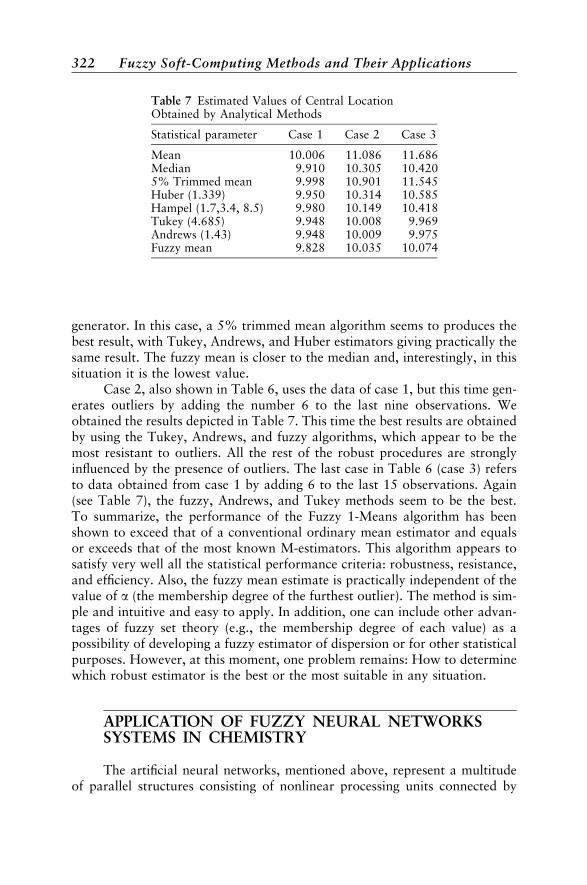
generator. In this case, a 5% trimmed mean algorithm seems to produces thebest result, with Tukey, Andrews, and Huber estimators giving practically thesame result. The fuzzy mean is closer to the median and, interestingly, in thissituation it is the lowest value.

Case 2, also shown in Table 6, uses the data of case 1, but this time gen-erates outliers by adding the number 6 to the last nine observations. Weobtained the results depicted in Table 7. This time the best results are obtainedby using the Tukey, Andrews, and fuzzy algorithms, which appear to be themost resistant to outliers. All the rest of the robust procedures are stronglyinfluenced by the presence of outliers. The last case in Table 6 (case 3) refersto data obtained from case 1 by adding 6 to the last 15 observations. Again(see Table 7), the fuzzy, Andrews, and Tukey methods seem to be the best.To summarize, the performance of the Fuzzy 1-Means algorithm has beenshown to exceed that of a conventional ordinary mean estimator and equalsor exceeds that of the most known M-estimators. This algorithm appears tosatisfy very well all the statistical performance criteria: robustness, resistance,and efficiency. Also, the fuzzy mean estimate is practically independent of thevalue of a (the membership degree of the furthest outlier). The method is sim-ple and intuitive and easy to apply. In addition, one can include other advan-tages of fuzzy set theory (e.g., the membership degree of each value) as apossibility of developing a fuzzy estimator of dispersion or for other statisticalpurposes. However, at this moment, one problem remains: How to determinewhich robust estimator is the best or the most suitable in any situation.

APPLICATION OF FUZZY NEURAL NETWORKSSYSTEMS IN CHEMISTRY

The artificial neural networks, mentioned above, represent a multitudeof parallel structures consisting of nonlinear processing units connected by

Table 7 Estimated Values of Central LocationObtained by Analytical Methods

Statistical parameter Case 1 Case 2 Case 3

Mean 10.006 11.086 11.686Median 9.910 10.305 10.4205% Trimmed mean 9.998 10.901 11.545Huber (1.339) 9.950 10.314 10.585Hampel (1.7,3.4, 8.5) 9.980 10.149 10.418Tukey (4.685) 9.948 10.008 9.969Andrews (1.43) 9.948 10.009 9.975Fuzzy mean 9.828 10.035 10.074


links of different weights. Because of their good ability to approximate func-tional dependencies between descriptive parameters and responses of a com-plex system, ANNs are widely employed for solving recognition problemsand quantitative relationships. If we suppose an infinite or large-enough dataset, a simple ANN model can provide a satisfactory degree of generalization.However, in real situations one usually deals with restricted sets of trainingsamples. Once trained, neural networks are quick and have a tolerance toincomplete or noisy data, which makes them useful in real-world environments.

Within the field of chemistry, various applications have already beenpublished. Jansson114 and Zupan and Gasteiger115 published an overview ofan MLP (multilayer perceptron), that is trained by back-propagation of errors,and other types of neural networks. However, the basic source in this fieldcontinues to be the well-known book of Zupan and Gasteiger.116 In analyticalchemistry, neural networks have been applied to pattern recognition, modeling,and prediction, for example, in multicomponent analysis or process control,to classification, clustering and pattern association.117–122

It is abundantly clear that fuzzy logic is better able to represent humanknowledge in a form of rules while ANNs are better able to learn from exam-ples. As a consequence of their complementary properties, then, extensiveefforts are being made to combine fuzzy theory and neutral networks to profitfrom the advantages of each while trying to bypass the disadvantages of theisolated techniques.123–125

A fuzzy neural network blends elements of fuzzy and neural networkcomputations into a single connectionist architecture. In general terms, twodifferent types of neural-fuzzy hybrids have emerged: one that uses neural net-works to derive the parameters of a fuzzy system, and another that provides animplementation of a fuzzy system within one neural network architecture. Aneural fuzzy system is a fuzzy system that uses a learning algorithm derivedfrom or inspired by neural network theory to determine its parameters (fuzzysets and fuzzy rules) by processing data samples. Neural-fuzzy systems can beused to derive solutions involving the neural network’s advantages of model-free learning, good generalization, and powerful nonlinear mapping capabil-ities. The primary strength obtained from the fuzzy logic component is asystem that can both be initialized by the existing semantic knowledge, andhave structured information (knowledge) extracted from it in an interpretableformat. Thus, the ‘‘black-box’’ difficulty, which is widely regarded as a prin-ciple weakness of neural networks, can be lessened. A series of steps exist toimplement a basic neural fuzzy system: (1) convert real-valued data into a fuz-zified representation; (2) train the fuzzified information with a neural network;and then (3) defuzzify the result to produce real values of the desired output.After the system is trained to satisfaction, fuzzy rules can be extracted from thetrained neural network.

A fuzzy multivariate rule-building expert system (FuRES) has beendevised that also functions as a minimal neural network.126 This system builds

Application of Fuzzy Neural Networks Systems in Chemistry 323

from training sets of data that use feature transformation in their antecedents.The rules are constructed using the ID3 algorithm with a fuzzy expression ofclassification entropy. The rules are optimal with respect to fuzziness and canaccommodate overlapped and underlapped clusters of data. Otto127 appliedfuzzy associative memory (FAM) developed by Kosko128 for the interpretationof UV spectra and Harrington and Wabuyele129 devised a fuzzy optimal asso-ciative memory (FOAM) for background correction of near-IR spectra. TheFOAM technique uses enhanced optimal associative memory (OAM) and afuzzy function for encoding the spectra.

Agapito et al.130 applied fuzzy logic to an array of semiconductor gassensors to analyze different atmospheres for the different gases and Ottoet al.131 developed a scheme based on the principles of fuzzy logic that makesuse of various pieces of information available either from spectroscopicknowledge or from the particular spectrum that requires evaluation. A fuzzyexpert system has also been successfully developed for the automated qualita-tive and semiquantitative interpretation of X-ray diffraction spectra,132 auto-mation of matrix-assisted laser desorption–ionization mass spectrometry(MALDI),133 and for polymer analysis.134

Very efficient and promising applications of fuzzy expert systems werealso discussed concerning, for example, the optimization of glutamic acid pro-duction,135 control of penicillin concentration in a fed-batch bioreactor,136,137

and, last but not the least, a fuzzy logic approach to analyzing gene expressiondata.138 Finally, two different soft computing techniques (a competitive learn-ing neural network and an integrated neural network-fuzzy logic-genetic algo-rithm approach) were employed in the analysis of a database subset obtainedfrom the Cambridge Structural Database.139

APPLICATIONS OF FUZZY SETS THEORY ANDFUZZY LOGIC IN THEORETICAL CHEMISTRY

In our opinion, all major theoretical aspects including some practicalapplications of fuzzy theory in the field of Theoretical Chemistry are verywell illustrated in the book edited by Rouvray.140 The nine contributors tothis book, research chemists and mathematicians, explain the foundations offuzzy logic and its growing importance in the physical sciences, describe mole-cular sizes and shapes, define chemical concepts such as chirality and the roleof quantum chemical species and systems, and outline the engineering of mole-cular species, including drug design. More recently, an excellent exploration ofthe role of fuzzy methods in chemistry providing theoretical background aswell as descriptions of practical applications in all the significant areas ofchemistry was also published in the Encyclopedia of Computational Chemis-try by Ehrentreich.141


CONCLUSIONS AND REMARKS

Soft computing has become an important computational paradigm dueto many factors. On the one hand, it is tolerant of imprecision, uncertainty,and partial truth, properties that do not generally hold for hard computingtechniques. On the other hand, soft computing is formed by a set of theories(fuzzy logic, neural networks, evolutionary algorithms) that, even if quite dis-tinct from each other, with different aims and methods, can be combined togenerate hybrid approaches, which are more powerful than their individualcounterparts. Being a theory that deals with imprecision, uncertainty, and par-tial truth, soft computing is suitable to model problems from a large number offields. In this chapter, we presented an introduction to different soft computingmethods, and reviewed the applications of soft computing (with a focus onfuzzy methods) in chemistry and related fields. We hope that this work willprove to be useful in research efforts directed toward integrating soft comput-ing methodologies with chemistry and chemical engineering issues and problems.

REFERENCES

1. T. Kohonen, Self-Organizing Maps, Second Extended Edition, Springer Series in InformationSciences, Vol. 30, Springer-Verlag, Berlin/Heidelberg, New York, 1995, 1997.

2. S. Kaski, Data Exploration Using Self-Organizing Maps, Ph.D. Dissertation, Neural Net-works Research Center, Helsinki University of Technology, 1997.

3. T. Honkela, Self Organizing Maps in Natural Language Processing, Ph.D. Dissertation,Neural Networks Research Center, Helsinki University of Technology, 1997.

4. L. A. Zadeh, Inform. Control., 8, 338 (1965). Fuzzy Sets.

5. H. F. Pop, Intelligent Systems in Classification Problems, Ph.D. Dissertation, Babes-BolyaiUniversity, Cluj-Napoca, Romania, 1995.

6. M. Meloun, M. Militky, and M. Forina, Chemometrics for Analytical Chemistry, Vol. I: PC-aided Statistical Data Analysis, Ellis Horwood, Chichester, 1992.

7. D. L. Massart, B. G. M. Vandeginste, S. N. Deming, Y. Michotte, and L. Kaufman,Chemometrics: A Textbook, Elsevier, Amsterdam, The Netherlands, 1988.

8. D. L. Massart and L. Kaufman, The Interpretation of Analytical Chemical Data by the Use ofCluster Analysis, Wiley, New York, 1983.

9. P. E. T. Auf der Heyde, J. Chem. Educ., 67, 461 (1990). Analyzing Chemical Data in MoreThan Two Dimensions.

10. P. S. Shenkin and D. Q. McDonald, J. Comput. Chem., 15, 899 (1994). Cluster Analysis ofMolecular Conformations.

11. J. Einax, H. W. Zwanziger, and S. Geiß, Chemometrics in Environmental Analysis, Wiley,Chichester, 1997.

12. M. Otto, Chemometrics: Statistics and Computer Application in Analytical Chemistry, Wiley-VCH, Weinheim, 1998.

13. Y-H. Pao, Adaptive Pattern Recognition and Neural Networks, Addison-Wesley PublishingCompany, 1989.

14. R. Fuller, Introduction to Neuro-Fuzzy Systems, Advances in Soft Computing Series, Springer-Verlag, Berlin/Heidelberg, 1999.

References 325

15. C. D. G. Jondarr, Backpropagation Family Album, Department of Computing, MacquarieUniversity, Australia, Technical Report C/TR96-05, 1996.

16. D. R. Tveter, Backpropagator’s Review, http://www.dontveter.com

17. K. Gurney, An Introduction to Neural Networks, UCL Press, London, 1996.

18. Z. Michalewicz, Genetic Algorithms þ Data Structures ¼ Evolution Programs, Third,Revised and Extended Version, Springer-Verlag, Berlin 1996.

19. M. Tomassini, A Survey of Genetic Algorithms, Volume III of Annual Reviews of Computa-tional Physics, World Scientific, Singapore, 1995.

20. T. Back and H. P. Schwefel, in Genetic Algorithms in Engineering and Computer Science,J. Periaux and G. Winter, Eds., Wiley, New York, 1995. Evolution Strategies I: Variantsand their Computational Implementation.

21. H. P. Schwefel and Thomas Back, in Genetic Algorithms in Engineering and ComputerScience, J. Periaux and G. Winter, Eds., Wiley, 1995. Evolution Strategies II: TheoreticalAspects.

22. T. Back, G. Rudolph, and H. P. Schwefel, in Proceedings of the Second Annual Conference onEvolutionary Programming, Evolutionary Programming Society, D. F. Fogel and W. Atmar,Eds., San Diego, CA, 1993, pp. 11–22, Evolutionary Programming and Evolution Strategies:Similarities and Differences.

23. G. J. Klir and B. Yuan, Fuzzy Sets and Fuzzy Logic, Prentice-Hall, New Jersey, 1995.

24. J. C. Bezdek, Pattern Recognition with Fuzzy Objective Function Algorithms, Plenum Press,New York, 1987.

25. R. Lowen, Fuzzy Set Theory, Kluwer Academic Publishers, Amsterdam, 1995.

26. H. J. Zimmermann, Fuzzy Set Theory-and Its Applications, Kluwer Academic Publishers,Dordrecht, The Netherlands, 1996.

27. K. Tanaka, An Introduction to Fuzzy Logic for Practical Applications, Springer-Verlag,New York, 1997.

28. C. Saarbu, D. Dumitrescu, and H. F. Pop, Rev. Chim.(Bucharest), 44, 450 (1993). Applicationof Fuzzy Sets Theory in Thin Layer Chromatography.

29. D. Dumitrescu, C. Saarbu, and H. F. Pop, Anal. Lett., 27, 1031 (1994). A Fuzzy DivisiveHierarchical Clustering Algorithm for the Optimal Choice of Set of Solvent Systems.

30. H. F. Pop, D. Dumitrescu, and C. Saarbu, Anal. Chim. Acta, 310, 269 (1995). A Study ofRoman Pottery (terra sigillata) Using Hierarchical Fuzzy Clustering.

31. D. Dumitrescu, H. F. Pop, and C. Saarbu, J. Chem. Inf. Comput. Sci., 35, 851 (1995). FuzzyHierarchical Cross-Classification of Greek Muds.

32. H. F. Pop, C. Saarbu, O. Horowitz, and D. Dumitrescu, J. Chem. Inf. Comput. Sci., 36, 465(1996). A Fuzzy Classification of the Chemical Elements.

33. C. Saarbu, O. Horowitz, and H. F. Pop, J. Chem. Inf. Comput. Sci., 36, 1098 (1996). A FuzzyCross-Classification of Chemical Elements, Based on Their Physical, Chemical and Struc-tural Features.

34. H. F. Pop and C. Saarbu, Anal. Chem., 68, 771 (1996). A New Fuzzy Regression Algorithm.

35. C. Saarbu and H. F. Pop, Rev. Chim.(Bucharest), 48, 732 (1997). Fuzzy Regression.1.Heteroscedasticity.

36. H. F. Pop and C. Saarbu, Rev. Chim.(Bucharest), 48, 888 (1997). Fuzzy Regression. 2. Outliers.

37. H. F. Pop and C. Saarbu, J. Chem. Inf. Comput. Sci., 37, 510 (1997). The Fuzzy HierarchicalCross-Classification Algorithm. Improvements and Comparative Study.

38. J. C. Bezdek, C. Coray, R. Gunderson, and J. Wantson, SIAM J. Appl. Math., 40, 339 (1981).Detection and Characterisation of Cluster Substructure: I. Linear Structure: Fuzzy C-lines.

39. J. C. Bezdek, C. Coray, R. Gunderson, and J. Wantson, SIAM J. Appl. Math., 40, 358 (1981).Detection and Characterization of Cluster Substructure: II. Linear Structure: FuzzyC-Varieties and Convex Combinations Thereof.


40. T. R. Cundari, C. Saarbu, and H. F. Pop, J. Chem. Inf. Comput. Sci., 42, 1363 (2002). RobustFuzzy Principal Component Analysis (FPCA). A Comparative Study Concerning Interactionof Carbon–Hydrogen Bonds with Molybdenum–Oxo Bonds.

41. D. Driankov, H. Hellendoorn, and M. Reinfrank, An Introduction to Fuzzy Control,Springer-Verlag, New York, 1993.

42. W. Siler, Building Fuzzy Expert Systems, Birmingham, Alabama, http://users.aol.com/wsiler/

43. W. Pedrycz, Fuzzy Sets and Syst., 56, 1 (1993). Fuzzy Neural Networks and Neurocomputing.

44. D. Nauck, Proceedings of the Third European Congress on Intelligent Techniques andSoft-Computing (EUFIT ’95), Aachen (August 28–31, 1995), pp. 1159–1164. BeyondNeuro-Fuzzy: Perspectives and Directions.

45. T. Feuring and W. M. Lippe, Fuzzy Sets Syst., 102, 227 (1999). The Fuzzy Neural NetworkApproximation Lemma.

46. T. Bernd, M. Kleutges, and A. Kroll, Neural Computing Appl., 8, 151 (1999). Nonlinear BlackBox Modelling–Fuzzy Networks Versus Neural Networks.

47. W. Pedrycz, Soft Comput., 2, 61 (1998). Fuzzy Evolutionary Computing.

48. L.O. Hall, B. Ozyurt, and J.C. Bezdek, IEEE Trans. Evo. Comput., 3, 103 (1999). Clusteringwith a Genetically Optimized Approach.

49. A. Blanco, M. Delgado, and M.C. Pegalajar, Int. J. Approx. Reason., 23, 67 (2000). A GeneticAlgorithm to Obtain the Optimal Recurrent Neural Network.

50. R. Ostermark, Soft Comput., 3, 206 (1999). A Neuro-Genetic Algorithm for HeteroscedasticTime-Series Processes Empirical Tests on Global Asset Returns.

51. E. G. Mazurs, Types of Graphic Representations of The Periodic System Of ChemicalElements, La Grange, IL, 1959.

52. J. W. von Spronsen, The Periodic System of Chemical Elements. A History of the FirstHundred Years, Elsevier, Amsterdam, The Netherlands, 1959.

53. O. Horowitz, C. Saarbu, and H. F. Pop, Rev. Chim.(Bucharest), 51, 17 (2000). PatternRecognition Applied to Chemical Elements.

54. O. Horowitz, C. Saarbu, and H. F. Pop, Rationale Classification of Chemical Elements, DaciaPrinting House, Cluj-Napoca, Romania, 2000.

55. W. Preyer, Berliner Deut. Pharm. Ges., 2, 144 (1893). Das Genetische System der ChemischenElementen.

56. J. C. Bezdek, R. Ehrlich, and W. Full, Comput. Geosci., 10, 191 (1984). FCM: The Fuzzyc-Means Clustering Algorithm.

57. R. J. Mayer, Naturwissenschaften, 2, 781 (1914). Positions of the Rare Earth Elements in thePeriodic System.

58. H. Bassett, Chem. News, 65, 3, 19 (1892). A Tabular Expression of the Periodic Relations ofthe Elements.

59. J. W. van Spronsen, The Periodic System of Chemical Elements, Elsevier, Amsterdam, TheNetherlands, 1969.

60. J. D. Clark, J. Chem. Educ., 10, 675 (1933). A New Periodic Chart.

61. F. Scheele, Z. Naturforschung, 4a, 137 (1949). The Position of the Lanthanides and Actinidesin the Periodic Table.

62. T. Ternstrom, J. Chem. Educ., 41, 190 (1964). A Periodic Table.

63. W. B. Jensen, J. Chem. Educ., 59, 634 (1982). The Positions of Lanthanum (Actinium) andLutetium (Lawrencium) in the Periodic Table.

64. B. Earl and D. Wilford, Chemistry Data Book, Blackie, London, 1991.

65. D. R. Lide, Ed., CRC Handbook of Chemistry and Physics, 71st ed., CRC Press, Boca Raton,FL, 1990.

66. F. H. Allen and O. Kennard, Chem. Design Autom. News, 8, 31 (1993). 3D Search andResearch using the Cambridge Structural Database.

References 327

67. W. A. Nugent and J. M. Mayer, Metal-Ligand Multiple Bonds, Wiley, New York,1988.

68. J. M. Mayer, Acc. Chem. Res., 31, 441 (1998). Hydrogen Atom Abstraction by Metal–OxoComplexes: Understanding the Analogy with Organic Radical Reactions.

69. C. Saarbu and H. W. Zwanziger, Anal. Lett., 34, 1541 (2001). Fuzzy Classification andComparison of Some Romanian and German Mineral Waters.

70. V. Simeonov, H. Puxbaum, S. Tsakovski, C. Saarbu, and M. Kalina, Environmetrics, 10, 137(1999). Classification and Receptor Modeling of Wet Precipitation Data from CentralAustria (1984–1993).

71. G. N. Chen, Anal. Chim. Acta, 271, 115 (1993). Assessment of Environmental Water withFuzzy Cluster Analysis and Fuzzy Recognition.

72. S. Pudenz, R. Bruggemann, B. Luther, A. Kaune, and K. Kreimes, Chemosphere, 40, 1373(2000). An Algebraic/Graphical Tool to Compare Ecosystems with Respect to their PollutionV: Cluster Analysis and Hasse Diagrams.

73. H. van Malderen, S. Hoornaert, and R. van Grieken, Environ. Sci. Technol., 30, 489 (1996).Identification of Individual Aerosol Particles Containing Cr, Pb, and Zn Above the NorthSea.

74. A. Held, K. P. Hinz, A. Trimborn, B. Spengler, and O. Klemm, Aerosol Sci., 33, 581 (2002).Chemical Classes of Atmospheric Aerosol Particles at a Rural Site in Central Europe DuringWinter.

75. W. Jambers, A. Smekens, R. van Grieken, V. Shevchenko, and V. Gordeev, Colloids andSurfaces A: Physicochem. Eng. Aspects, 120, 61 (1997). Characterisation of ParticulateMatter from the Kara Sea Using Electron Probe X-ray Micro Analysis.

76. A. M. Lahdenpera, P. Tamminen, and T. Tarvainen, Appl. Geochem., 16, 123 (2001).Relationships Between Geochemistry of Basal Till and Chemistry of Surface Soil at ForestedSites in Finland.

77. J. A. Markus and A. B. McBratney, Aust. J. Soil Res., 34, 453 (1996). An Urban Soil Study:Heavy Metals in Glebe, Australia.

78. F. D. Tamas, J. Abonyi, J. Borszeki, and P. Halmos, Cem. Conc. Res., 32, 1325 (2002). TraceElements in Clinker II. Qualitative Identification by Fuzzy Clustering.

79. J. Finol, Y. K. Guo, and X. D. Jing, J. Petrol. Sci. Eng., 29, 97 (2001). A Rule Based FuzzyModel for the Prediction of Petrophysical Rock Parameters.

80. J. R. Perez-Correra, M. V. Letelier, A. Cipriano, H. Jorquera, O. Encalada, and I. Solar, in AirPollution VI, C. A. Brebbia, C. F. Ratto, and H. Power, Eds., WIT Press, Southampton,UK, 1998, pp. 257–266. Forecasting High SO2 Concentration Levels with Fuzzy ClusteringTechniques.

81. K. P. Hinz, M. Greweling, F. Drews, and B. Spengler, J. Am. Soc. Mass Spectrom., 10, 648(1999). Data Processing in On-Line Laser Mass Spectrometry of Inorganic, Organic, orBiological Airborne Particles.

82. P. Samaras, A. Kungolos, T. Karakasidis, D. Georgiou, and K. Perakis, J. Environ. Sci. Health,A, 36, 153 (2001). Statistical Evaluation of PCDD/F Emission Data During Solid WasteCombustion by Fuzzy Clustering Techniques.

83. C. Saarbu and H. F. Pop, Chemosphere, 40, 513 (2000). Fuzzy Classification of the First 10MEIC.

84. D. Melcher and M. Matthies, Ecol. Model., 85, 41 (1996). Application of Fuzzy Clustering toData Dealing with Phytotoxicity.

85. M. Friederichs, O. Franzle, and A. Salski, Ecol. Model., 85, 27 (1996). Fuzzy Clustering ofExisting Chemicals According to Their Ecotoxicological Properties.

86. J. C. Frisvad, Chem. Intell. Lab. Syst., 14, 253 (1992). Chemometrics and Chemotaxonomy: AComparison of Multivariate Statistical Methods for the Evaluation of Binary FungalSecondary Metabolite Data.


87. A. Linusson, S. Wold, and B. Norden, Chem. Intell. Lab. Syst., 44, 213 (1998). FuzzyClustering of 627 Alcohols, Guided by a Strategy for Cluster Analysis of ChemicalCompounds for Combinatorial Chemistry.

88. F. Ros, K. Audouze, M. Pintore, and J. R. Chretien, SAR and QSAR Environ. Res., 11, 281(2000). Hybrid Systems for Virtual Screening: Interest of Fuzzy Clustering Applied toOlfaction.

89. T. Blaffert, Anal. Chim. Acta, 161, 135 (1984). Computer-Assisted Multicomponent SpectralAnalysis with Fuzzy Data Sets.

90. A. R. Goss and M. J. Adams, Anal. Proceedings, Anal. Commun., 31, 23 (1994). SpectralRetrieval by Fuzzy Matching.

91. F. Ehrentreich, Fresenius J. Anal. Chem., 357, 527 (1997). Representation of ExtendedInfrared Spectrum-Structure-Correlations Based on Fuzzy Theory.

92. F. Ehrentreich, Fresenius J. Anal. Chem., 359, 56 (1997). Derivation of Substructures fromInfrared Band Shapes by Fuzzy Logic and Partial Cross Correlation Functions.

93. S. Kokot, S. Carswell, and D. L. Massart, Appl. Spectrosc., 46, 1393 (1992). Application ofDRIFT Spectroscopy for Comparison of Dye Mixtures Extracted from Small TextileSamples.

94. M. Otto and H. Bandemer, Anal. Chim. Acta, 184, 21 (1986). Pattern Recognition Based onFuzzy Observations for Spectroscopic Quality Control and Chromatographic Fingerprinting.

95. M. Otto and H. Bandemer, Anal. Chim. Acta, 191, 193 (1986). A Fuzzy Method forComponent Identification and Mixture Evaluation in the Ultraviolet Spectral Range.

96. M. Otto, W. Wegscheider, and E. P. Lankmayr, Anal. Chem., 60, 517 (1988). A FuzzyApproach to Peak Tracking in Chromatographic Separations.

97. U. Horchner and M. Otto, Fresenius J. Anal. Chem., 344, 217 (1992). Identification of UV/VIS-Spectra Based on a Fuzzy Function.

98. Y. Gu, C. Hirano, and M. Horiike, Rapid Commun. Mass Spectrom., 5, 622 (1991). FuzzyClassificational Analysis of Continuously Scanned Mass Spectra of Binary Mixtures ofPositionally Isomeric Tetradecenols.

99. Y. Gu, Fresenius J. Anal. Chem., 354, 241 (1996). Identification of the Configuration of SexPheromones with a Conjugated Double Bond by Fuzzy Similarity Analysis of Chemical Shiftsof Olefinic Carbons.

100. J. Xu, S. K. Straus, and B. C. Sanctuary, J. Chem. Inf. Comput. Sci., 33, 668 (1993).Automation of Protein 2D Proton NMR Assignment by Means of Fuzzy Mathematicsand Graph Theory.

101. M. Otto, G. Stingeder, K. Piplits, M. Grasserbauer, and M. Heinrich, Mikrochim. Acta, 106,163 (1992). Comparison of Depth Profiles in SIMS by a Fuzzy Method.

102. C. Saarbu, Anal. Lett. 28, 2077 (1995). A Comparative Study of Regression ConcerningWeighted Least Squares Methods.

103. C. Saarbu and G. Cımpan, J. Planar Chromatogr., 9, 126 (1996). Determination of Some 1,4-Benzodiazepines by Quantitative TLC. A Comparative Study Concerning Ladder of Power.

104. C. Saarbu, Croat. Chem. Acta, 70, 795 (1997). A New Median-Based Regression Method.

105. H. W. Zwanziger and C. Saarbu, Anal. Chem., 70, 1277 (1998). Validation of AnalyticalMethods Using Regression Procedure.

106. S. I. Pop, V. Pop, S. Cobzac, and C. Saarbu, J. Chem. Inf. Comput. Sci., 40, 91 (2000). Use ofWeighted Least–Squares Splines for Calibration in Analytical Chemistry.

107. H. Tanaka, S. Uejima, and K. Asai, IEEE Trans. Syst. Man and Cybernetics, SMC-12, 903(1982). Linear Regression Analysis with Fuzzy Model.

108. H. Otto and H. Bandemer, Chem. Intell. Lab. Syst., 1, 71 (1986). Calibration with ImpreciseSignals and Concentrations Based on Fuzzy Theory.

109. Y. Hu, J. Smeyers-Verbeke, and D. L. Massart, Chem. Intell. Lab. Syst., 8, 143 (1990). AnAlgorithm for Fuzzy Linear Calibration.

References 329

110. Y. Hu, J. Smeyers-Verbeke and D. L. Massart, Chem. Intell. Lab. Syst., 9, 31 (1990). OutliersDetection in Calibration.

111. T. Shimosaka, T. Kitamori, A. Harata, and T. Sawada, Anal. Sci., 7, 1389 (1991). FuzzyTreatement of Analytical Data for Colorimetry.

112. C. Saarbu and H. F. Pop, Talanta, 40, 513 (2001). Fuzzy Robust Estimation of Central Location.

113. P. L. Davies, Fresenius J. Anal. Chem., 331, 513 (1988). Statistical Evaluation of Inter-laboratory Tests.

114. P. A. Jansson, Anal. Chem., 63, 357A (1991). Neural Networks: An Overview.

115. J. Zupan and J. Gasteiger, Anal. Chim. Acta, 248, 1 (1991). Neural Networks: A New Methodfor Solving Chemical Problems or Just a Passing Phase?

116. J. Zupan and J. Gasteiger, Neural Networks for Chemists, VCH, Weinheim, 1993.

117. M. Otto, T. George, C. Schierle, and W. Wegscheider, Pure Appl. Chem., 64, 497 (1992).Fuzzy Logic and Neural Networks—Applications to Analytical Chemistry.

118. P. J. Gemperline, J. R. Long, and V. G. Gregoriou, Anal. Chem., 63, 2313 (1991). NonlinearMultivariate Calibration Using Principal Components Regression and Artificial NeuralNetworks.

119. J. R. Long, H. T. Mayfield, and M. V. Henley, Anal. Chem., 63, 1256 (1991). PatternRecognition of Jet Fuel Chromatographic Data by Artificial Networks with Back-Propaga-tion of Error.

120. D. N. Rassokhin, V. S. Lobanov, and D. K. Agrafiotios, J. Comput. Chem., 22, 373 (2001).Nonlinear Mapping of Massive Data Sets by Fuzzy Clustering and Neural Networks.

121. H. Sundgren, I. Lundstrom, and H. Vollmer, Sensors and Actuators, 6, 225 (1984). ChemicalSensor Arrays and Abductive Networks.

122. H. Sundgren, F. Winquist, I. Lukkart, and I. Lundstrom, Meas. Sci. Technol., 2, 464 (1991).Artificial Neural Networks and Gas Sensor Arrays: Quantification of Individual Compo-nents in a Gas Mixture.

123. P. B. Harrington, Chem. Intell. Lab. Syst., 18, 157 (1993). Minimal Neural Networks:Concerted Optimization of Multiple Decision Planes.

124. P. B. Harrington, Chem. Intell. Lab. Syst., 19, 143 (1993). Minimal Neural Networks:Differentiation of Classification Entropy.

125. P. B. Harrington and B. W. Pack, Anal. Chim. Acta, 277, 189 (1993). FLIN: Fuzzy LinearInterpolating Network.

126. P. B. Harrington, J. Chemom., 5, 467 (1991). Fuzzy Multivariate Rule-Building ExpertSystems: Minimal Neural Networks.

127. M. Otto, Anal. Chem., 62, 797A (1990). Fuzzy Sets: Applications to Analytical Chemistry.

128. B. Kosko, Neural Networks and Fuzzy Systems, Prentice-Hall, Englewood Cliffs, NJ, 1992.

129. B. W. Wabuyele and P. B. Harrington, Appl. Spectrosc., 50, 35 (1996). Fuzzy OptimalAssociative Memory for Background Prediction of Near-Infrared Spectra.

130. J. A. Agapito, L. Agapito, M. Schneider, R. Garcia Rosa, and T. Pedro, Sensors and ActuatorsB, 15–16, 105 (1993). Fuzzy Logic Applied to Gas Sensors.

131. R. Neubock, W. Wegscheider, and M. Otto, Microchem. J., 45, 343 (1992). AutomatedQualitative Analysis by Inductively Coupled Plasma Atomic Emission Spectrometry Basedon a Fuzzy Reasoning Scheme.

132. B. Adler, P. Schutze, and J. Will, Anal. Chim. Acta, 271, 287 (1993). Expert System forInterpretation of x-Ray Diffraction Spectra.

133. O. L. Jensen, P. Mortensen, O. Vorm, and M. Mann, Anal. Chem., 69, 1706 (1997).Automation of Matrix-Assisted Laser Desorption/Ionization Mass Spectrometry UsingFuzzy Logic Feedback Control.

134. D. J. Ramsbottom and M. J. Adams, Chem. Intell. Lab. Syst., 19, 53 (1993). Uncertaintywithin a Commercial Expert System Shell for Polymer Analysis.


135. M. Kishimoto, M. Moo-Young, and P. Allsop, Bioprocess Eng., 6, 163 (1991). A Fuzzy ExpertSystem for the Optimization of Glutamic Acid Production.

136. V. G. Nyttle and M. Chidambaram, Bioprocess Eng., 9, 115 (1993). Fuzzy Logic Control of aFed-Batch Fermentor.

137. M. Ronen, Y. Shabtai, and H. Guterman, Biotechnol. Bioeng., 77, 420 (2002). Hybrid ModelBuilding Methodology Using Unsupervised Fuzzy Clustering and Supervised Neural Net-works.

138. P. J. Woolf and Y. Wang, Physiol Genomics, 3, 9 (2000). A Fuzzy Logic Approach toAnalyzing Gene Expression Data.

139. T. R. Cundari and M. Russo, J. Chem. Inf. Comput. Sci., 41, 281 (2001). Database MiningUsing Soft Computing Techniques. An Integrated Neural Network-Fuzzy Logic-GeneticAlgorithm Approach.

140. D. H. Rouvray, Ed., Fuzzy Logic in Chemistry, Academic, San Diego, 1997.

141. F. Ehrentreich, in Encyclopedia of Computational Chemistry, P. Schleyer, Ed., Wiley,Chichester, 1998, pp. 1090–1103. Fuzzy Methods in Chemistry.

References 331

CHAPTER 6

Development of ComputationalModels for Enzymes, Transporters,Channels, and Receptors Relevant toADME/Tox

Sean Ekins*a and Peter W. Swaan{

*GeneGo, 500 Renaissance Drive, Suite 106, St. Joseph, MI49085yDepartment of Pharmaceutical Sciences, University of Maryland,HSF2 20 Penn Street, Baltimore, MD 21201

INTRODUCTION

ADME/Tox Modeling: An Expansive Vision

Proteins may be classified primarily by their sequence or by their func-tion, which may include acting as enzymes, transporters, channels, and recep-tors (a comprehensive and detailed review would be well beyond the scope of asingle book chapter). An alternative way of classifying proteins is to considerthe influence they have on drug Absorption, Metabolism, Distribution, Excre-tion, and Toxicology (ADME/Tox). A complete picture of any one proteinsystem from expression, regulation, substrate and inhibitor selectivity, orprotein–protein interaction is not currently feasible. We are therefore left



aAuthor for correspondence. Phone: 269-983-7649, Fax: 269-983-7654,

Email: [email protected]

333

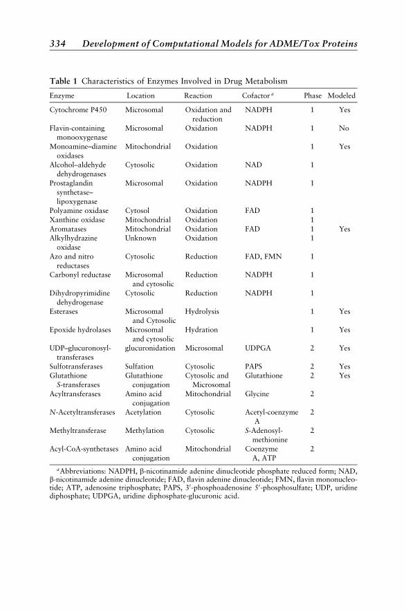
Table 1 Characteristics of Enzymes Involved in Drug Metabolism

Enzyme Location Reaction Cofactor a Phase Modeled

Cytochrome P450 Microsomal Oxidation and NADPH 1 Yes

reduction

Flavin-containing Microsomal Oxidation NADPH 1 Nomonooxygenase

Monoamine–diamine Mitochondrial Oxidation 1 Yes

oxidases

Alcohol–aldehyde Cytosolic Oxidation NAD 1dehydrogenases

Prostaglandin Microsomal Oxidation NADPH 1

synthetase–

lipoxygenasePolyamine oxidase Cytosol Oxidation FAD 1

Xanthine oxidase Mitochondrial Oxidation 1

Aromatases Mitochondrial Oxidation FAD 1 YesAlkylhydrazine Unknown Oxidation 1

oxidase

Azo and nitro Cytosolic Reduction FAD, FMN 1

reductasesCarbonyl reductase Microsomal Reduction NADPH 1

and cytosolic

Dihydropyrimidine Cytosolic Reduction NADPH 1

dehydrogenaseEsterases Microsomal Hydrolysis 1 Yes

and Cytosolic

Epoxide hydrolases Microsomal Hydration 1 Yes

and cytosolicUDP–glucuronosyl- glucuronidation Microsomal UDPGA 2 Yes

transferases

Sulfotransferases Sulfation Cytosolic PAPS 2 YesGlutathione Glutathione Cytosolic and Glutathione 2 Yes

S-transferases conjugation Microsomal

Acyltransferases Amino acid Mitochondrial Glycine 2

conjugationN-Acetyltransferases Acetylation Cytosolic Acetyl-coenzyme 2

A

Methyltransferase Methylation Cytosolic S-Adenosyl- 2

methionineAcyl-CoA-synthetases Amino acid Mitochondrial Coenzyme 2

conjugation A, ATP

aAbbreviations: NADPH, b-nicotinamide adenine dinucleotide phosphate reduced form; NAD,b-nicotinamide adenine dinucleotide; FAD, flavin adenine dinucleotide; FMN, flavin mononucleo-tide; ATP, adenosine triphosphate; PAPS, 30-phosphoadenosine 50-phosphosulfate; UDP, uridinediphosphate; UDPGA, uridine diphosphate-glucuronic acid.

334 Development of Computational Models for ADME/Tox Proteins

with a fragmented research area containing many individual proteins fromwhich limited inferences can be drawn. What follows is an admittedly selectivereview on the current status of ADME/Tox for several intensely studied pro-teins in the hope that it will stimulate other investigators to think beyond indi-vidual proteins and adopt a more unified and holistic perspective in theirresearch. In many cases, there may exist fundamental linkages between eachclass of protein for which the same computational tools can be applied tounravel the intricacies of each individual system; this will become the commonthread interweaving through the fabric of this chapter. To our knowledge, nosingle laboratory has developed computational models for each ADME/Toxsystem described herein (although this may be currently underway). Withoutmodels for every system an initial barrier exists to their successful integrationand the genesis of a complete prediction for ADME/Tox. To date, there havebeen many reviews on ADME/Tox modeling,1–4 which should be refered tofor more details on modeling general processes like blood–brain barrier(BBB) transport, absorption, and bioavailability.

The Concerted Actions of Transport and Metabolism

It is generally accepted that mammalian physiology has evolved mechan-isms to specifically uptake essential nutrients and to remove hydrophobicxenobiotic and endobiotic molecules to prevent their accumulation and even-tual toxicity. Important components of this process are metabolism and trans-port. There has been a dramatic increase in our understanding of these fieldsover the past decade, predominantly influenced by molecular biology, theisolation and expression of these proteins, and improvements in both thesensitivity and throughput of analytical and experimental technologies.

Metabolism

Metabolism can be defined as what the body does to convert a moleculeto a more readily excreted one. Such molecules can actually become more bio-logically active via metabolism (which occurs for some pro-carcinogens, forexample) and this kind of activation may be taken advantage of when design-ing prodrugs. In many species, metabolism is specifically enzymatic in naturesuch that a protein other than the desired target may bind the drug, and there-after a cofactor-catalyzed reaction can remove or add a functional group to thedrug molecule. Table 1 compiles the majority of enzymes, and describes theirintracellular localization, cofactors, and functionalization pathways. Themajor enzymes involved in drug metabolism, like cytochromes P450 (CYP)and UDP-glucuronosyl transferases (UDPGT), are predominantly localizedwithin the endoplasmic reticulum of cells and are relatively straightforwardto study in vitro (reviewed in Ref. 5). These types of enzyme-catalyzed drugmetabolism pathways may occur within many tissues in the body or theymay be localized in just one cell type. Where these pathways exist is very

Introduction 335

much dependent on the relative expression levels of the enzymes in a particulartissue although, in general, the liver and intestine contain the highest levels ofmost drug metabolizing enzymes.

The CYPs represent a very large superfamily of heme-containingenzymes that can either oxidize or reduce a large number of structurally dif-ferent endogenous and exogenous molecules because of their broad substratespecificity and their regio- and stereoselectivity. These enzymes are ubiqui-tously expressed and they may be induced by drugs and endobiotics as wellas by other environmental xenobiotics. Of increasing importance to our under-standing of ADME/Tox is the role of enzymes in drug–drug interactions, inwhich one drug may interfere with the metabolism of another drug if theycompete to fit (preferably) within the same ligand-binding site of the sameenzyme. Among the endobiotics are the abundant steroids, and the bile acidsthat have essential roles as hormones, signaling molecules, and as detergents.However, we are now beginning to further understand how multiple endobio-tics, xenobiotics, therapeutic, and environmental agents may interfere with theremoval and metabolic mechanisms in vivo having potentially undesirabletoxic consequences. The role of CYPs probably began first as a functionalresponse for regulation of intracellular signals and further evolved to removeenvironmental molecules. In more popular terminology, it is believed thatCYPs have evolved from plant versus animal warfare.6

Transporters

The transport of a molecule into and out of cells, by both active trans-port and passive diffusion, is integral to xenobiotic and endobiotic metabo-lism. It is now well appreciated that organic solutes such as physiologicallycritical nutrients (amino acids, sugars, vitamins, and bile acids), as well as neu-rotransmitters and drugs, are transferred across cellular membranes by specia-lized transport systems.7 These systems encompass integral membraneproteins that shuttle substrates across the membrane, which is done by eithera passive process through channels (facilitated transporters) or by an activeprocess (via carriers). The latter is energized directly by the hydrolysis ofATP or indirectly by coupling to the cotransport of a counterion down its elec-trochemical gradient formed by Naþ, Hþ, or Cl�.

Our understanding of the biochemistry and molecular biology of mam-malian transport proteins has significantly advanced because of the develop-ment of expression cloning techniques. Initial studies in Xenopus laevisoocytes by Hediger et al.8,9 resulted in the isolation of the intestinal sodium-dependent glucose transporter, SGLT1. To date, sequence information andfunctional data derived from numerous transporters have revealed unifyingdesigns, similar energy-coupling mechanisms, and common evolutionary ori-gins.10 The plethora of isolated transporters motivated the human genenomenclature committee toclassify theseproteins intoadistinct genetic superfamily


named SLC (for SoLute Carrier). Currently, the SLC class contains 37 familieswith 205 members and is rapidly expanding (http://www.gene.ucl.ac.uk/nomenclature/). The ABC superfamily contains 7 families with 48 members;11

class B contains the well-known multidrug resistance gene (MDR1) derived P-glycoprotein (ABCB1), while class C comprises members of the multidrugresistance protein (MRP) subfamily. With the completion of the human gen-ome project, it can be anticipated that a vast number of membrane transportproteins will be identified without known physiological function. This clearlyraises questions that may be answered using computational technologies.

Transporters have a critical role in maintaining cellular homeostasis, andinterference with this delicate balance by xenobiotics including therapeuticsmay have an undesirable effect. On the other hand, the efficacy of drugsmay be improved by leveraging affinity for the transporters such that a drugcan piggyback with the physiological substrate, or at the very least, mimic itscritical molecular features.12–14 Efflux of molecules from cells therefore canoccur via transporters that would usually function to clear toxic endogenousmetabolites such as conjugated bile acids from the cell. One can therefore envi-sion that the enzymes involved in metabolism and the transporters have a veryclose linkage and functional regulation, working in concert to maintain thecellular steady state. Similarly, ion channels are key to maintaining cellularhomeostasis. Ion channels have important roles in cellular communicationand are critical to life. The up and down regulation of these proteins maybe under the control of many receptors that themselves can bind the same(or similar) molecules. These receptors likely have endogenous functions.Also, there are receptors with unrelated functions, such as those in the centralnervous system (CNS), which in some cases may have the same bindingrequirements as those of desirable non-CNS therapeutic targets. This, inturn, can lead to interactions that manifest as a neurological side effect, butthis area has been poorly explored. In its simplest sense, the common bindingrequirement across numerous proteins of different function and in multiplelocations represents a multidimensional problem that prevents our under-standing of whether or not a drug will impact each of these processes. How-ever, there are many transporters and enzymes of relevance for bothmetabolism and transport of drugs; understanding the effect a drug has onall of them represents a major challenge. This complicated ligand affinity pro-file determination is further compounded by the absence of freely availablecrystal structures for any of these membrane-bound proteins that are knownto bind drugs. If anything, our understanding of drug metabolism, transport,ion channel function, and the role of receptors (both CNS and non-CNS) isnow more complex than envisaged decades ago when far fewer of these pro-teins had been identified, sequenced, expressed, or analyzed in vitro or in vivo.

Consequently, the assessment of in vitro ADME/Tox parameters hasbeen moved much earlier in the pharmaceutical discovery process such that largeamounts of protein-specific data are generated. This data needs interpretation

Introduction 337

and that knowledge, in turn, may provide a valuable resource forgenerating computational models in the future. These ADME/Tox specificproteins can be viewed as ‘‘antitargets’’ in that they may need to be avoidedto some extent while the selection of molecules with a high affinity for thetherapeutic target(s), on the other hand, is critical. This chapter aims toshow novice molecular modelers what tools exist today for visualizing andmodeling enzymes, transporters, channels, and receptors that are relevant toADME/Tox with the goals of being able to design molecules that can leverageor avoid these antitargets as desired.

APPROACHES TO MODELING ENZYMES,TRANSPORTERS, CHANNELS, AND RECEPTORS

There have been considerable advances in the development of strategiesfor structure-based drug design. De novo molecule design, docking, and vir-tual combinatorial library generation have been recent hot topics in the litera-ture. Many publications in the mid-1990s outlined the successes andlimitations of all of these technologies.15–21 Computational approaches neededfor understanding metabolism and toxicology began to appear approximatelya decade after the evolution of computational tools used for assisting in targetprediction and optimization. Recently, several journal monographs have beendevoted to in silico modeling of ADME/Tox properties. In those monographsare numerous reviews providing useful information on the subject.1–3,22–30

During the past few years, we have seen researchers indicating that they cannow predict a molecule’s probability of success in vivo from simple chemico-physical descriptors.31,32 The development of in vitro assays, computationalprotocols, and the development of cheminformatics in the past decade havealso yielded data sets used to build specific computational models (Figure 1)

Figure 1 The in silico model building paradigm.


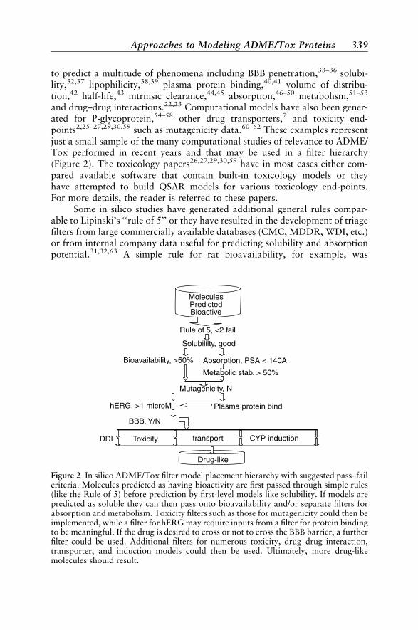
to predict a multitude of phenomena including BBB penetration,33–36 solubi-lity,32,37 lipophilicity,38,39 plasma protein binding,40,41 volume of distribu-tion,42 half-life,43 intrinsic clearance,44,45 absorption,46–50 metabolism,51–53

and drug–drug interactions.22,23 Computational models have also been gener-ated for P-glycoprotein,54–58 other drug transporters,7 and toxicity end-points2,25–27,29,30,59 such as mutagenicity data.60–62 These examples representjust a small sample of the many computational studies of relevance to ADME/Tox performed in recent years and that may be used in a filter hierarchy(Figure 2). The toxicology papers26,27,29,30,59 have in most cases either com-pared available software that contain built-in toxicology models or theyhave attempted to build QSAR models for various toxicology end-points.For more details, the reader is referred to these papers.

Some in silico studies have generated additional general rules compar-able to Lipinski’s ‘‘rule of 5’’ or they have resulted in the development of triagefilters from large commercially available databases (CMC, MDDR, WDI, etc.)or from internal company data useful for predicting solubility and absorptionpotential.31,32,63 A simple rule for rat bioavailability, for example, was

MoleculesPredictedBioactive

Drug-like

DDI Toxicity transport CYP induction

Plasma protein bindhERG, >1 microM

Mutagenicity, N

Bioavailability, >50%

Rule of 5, <2 fail

Solubililty, good

Absorption, PSA < 140A

BBB, Y/N

Metabolic stab. > 50%

Figure 2 In silico ADME/Tox filter model placement hierarchy with suggested pass–failcriteria. Molecules predicted as having bioactivity are first passed through simple rules(like the Rule of 5) before prediction by first-level models like solubility. If models arepredicted as soluble they can then pass onto bioavailability and/or separate filters forabsorption and metabolism. Toxicity filters such as those for mutagenicity could then beimplemented, while a filter for hERG may require inputs from a filter for protein bindingto be meaningful. If the drug is desired to cross or not to cross the BBB barrier, a furtherfilter could be used. Additional filters for numerous toxicity, drug–drug interaction,transporter, and induction models could then be used. Ultimately, more drug-likemolecules should result.

Approaches to Modeling ADME/Tox Proteins 339

described as being dependent on the polar surface area and number of rotat-able bonds of the administered drug.64 Similarly, there have been reasonablysuccessful studies directed at discriminating between drug-like and non-drug-like molecules,65,66 differentiating between leads and drugs,67 and describingcommon structural features of known drugs,68,69 as well as identifying mole-cules that are frequent or promiscuous hitters in high-throughput screens.70,71

The above mentioned triage-type filters represent an adequate first-level in sili-co screen, but they have some limitations and they do not adequately deal withthe overall ADME/Tox picture. These virtual approaches, however, representan effective and rapid means to filter and prioritize molecules based on desir-able structural descriptors or predicted simple physico-chemical properties.When combined with other computational or statistical approaches for select-ing molecules in a multivariate–multiobjective optimization22,25,72–74 one canavoid suboptimal molecules31 and shorten lead generation and lead optimiza-tion times.25 Ultimately these in silico models will enable us to increase thenumber of compounds that can be screened, if we use large virtuallibraries72,75,76 that can be scored for ADME/Tox and bioactivity. Now, wecan consider classical QSAR, pharmacophore, and homology modeling tech-niques that have been applied to modeling some of the proteins involved inADME/Tox.

Classical QSAR

The fundamentals, history, and methodology of QSAR and 3D-QSARhave been reviewed in considerable detail by Kubinyi, Waller and Oprea, aswell as by others. The reader is referred to these general overviews.77–79 Asearly as the 1960s it was appreciated that one could apply a mathematicalmodel to understand metabolic actions in order to design new or improveddrugs.80 One of the limitations of the QSAR method is the availability of large,adequate data sets. In the 1960s, the log P term alone was used in all equationsas a measure of hydrophobicity. It was found to be 2 for each system, suggest-ing that hydrophobicity was important for membrane penetration by a drug toreach the site of metabolism. Such studies were carried considerably further byHansch’s group,81–84 as well as by Lewis et al.85–93 in the metabolic field. Byadding other descriptors such as HOMO and LUMO (highest occupied andlowest unoccupied molecular orbitals, respectively), pKa, log D7.4, dipolemoment, solvent accessible surface area, volume of solvent accessible area,molecular length/width ratio, and molecular area/depth squared ratio, itbecame possible to further generate rough rules for the prediction of generalproperties displayed by substrates and inhibitors of each CYP.85,86 These clas-sical QSAR approaches for ADME/Tox properties have been updated to someextent by the utilization of newer three-dimensional (3D)-descriptors such asMS-WHIM.94–100 These and other developments now present us with a richsource of molecular descriptors for use with various QSAR technologies.


Finally, we should point out that while classical QSAR approaches generallyresult in a single equation with statistical terms, modern 3D-QSAR methodsgenerally produce graphically intensive models that may aid in the interpreta-tion of important features in molecular 3D space and the mapping back ofthese features onto the molecules of interest.

Pharmacophore Models

One of the alternatives to direct protein modeling is the determination ofa pharmacophore describing the features present within a ligand required forbioactivity. A pharmacophore is thus a representation of the spatial arrange-ment of structural features for a series of molecules (obtained after structurealignment and superposition) that show activity and affinity toward a protein.In some cases, the pharmacophore may be translated as a template for theactual binding site (though, depending on the software used, doing this is ques-tionable). The alignment of molecules based on chemical functionality allowsfor diverse and structurally unique molecules to be grouped together withoutthe need to perform an atom-by-atom comparison. A pharmacophore thusprovides a straightforward method for representing drug– enzyme interactionsthat does not directly represent the active site of the protein but instead impli-cates only the key features necessary for a particular biological response. Theprediction of interaction or activity for a novel molecule by a pharmacophorehypothesis is thus based on the geometric fit to the chemical features in thatpharmacophore. A recent book and a number of reviews describing pharma-cophore models exist.101–103 In our experience we have most frequently usedKm, Ki, IC50 (and less preferably percent inhibition) data when building phar-macophore models for ADME/Tox properties, although other valid types ofkinetic experimental values could also be used, such as dissociation constants.According to the literature, the two most commonly used programs for phar-macophore development are DISCO (DIStance COmparisons) and Catalyst.They are part of commercially available software suites and will be describedalong with other programs below. Note that public domain and pharmaceu-tical company specific proprietary softwares also exist.

CatalystCatalyst (Accelrys, San Diego, CA) is an integrated environment for con-

former generation using the poling technique (ConFirm),104 and pharmaco-phore alignment, automated hypothesis generation (HypoGen),105

pharmacophore, or molecular-shape based 3D searches. The softwarealso provides a useful way to generate simple initial models (HipHop) basedon a limited number of structures that could either be derived from X-ray con-formations or from low-energy conformers covering conformational space.106

The HipHop algorithm finds these models after a pruned exhaustive searchwhere it begins with a small set of features and then extends those features


until it cannot find a larger common configuration.106,107 The training setmembers must then map completely or partially on to the features in someconfiguration that the user can select. This technique is further described intwo detailed reviews,101,102 a schematic outlining these pharmacophoreapproaches is depicted in Figure 3.

To generate ADME/Tox pharmacophore models within Catalyst, ourresearch groups have mainly used the HypoGen function. Following the gen-eration of multiple conformers with ConFirm, HypoGen enables the genera-tion of structure–activity relationship pharmacophore (hypothesis) modelsfrom a defined set of molecules that possess biological activity values. Thehypotheses generated by HypoGen represent chemical features in 3D spacethat fit the features of the training set and are correlated with the biologicaldata within certain tolerances and weights. The hypotheses created by thealgorithm are pharmacophores that are generally common among the activemolecules but not among the inactive ones in the training set. The hypothesesare created after constructive, subtractive, and optimization phases.105 Theconstructive phase generates hypotheses common to the active molecules, byidentifying the actives, generating and storing all the hypotheses present in thetwo most active molecules, and then retaining the hypotheses that fit theremainder of the actives. In the subtractive phase, hypotheses are removedthat are unlikely to be useful if they are also found to be present in the inactive

Figure 3 A schematic for Catalyst pharmacophore generation.


compounds. A compound is deemed to be inactive if its activity is n orders ofmagnitude less active than the most active compound (where n is user deter-mined). Hypothesis optimization is performed using simulated annealing,which perturbs the hypotheses by rotating vector features and translatingother features at random in an attempt to improve the cost function. This algo-rithm accepts all improvements and some detrimental steps based on a prob-ability function and retains the 10 unique best scoring pharmacophores. Foreach of these 10 hypotheses, the activity of each training set molecule isregressed after fitting to the pharmacophore versus the observed activity. Aselected HypoGen hypothesis provides a means of predicting the biologicalactivity for additional molecules that have yet to be synthesized as well as a3D search query for databases.105

The creation of a pharmacophore model requires first generating multi-ple conformers of each molecule in an attempt to gather an extensive anddiverse coverage of conformational space. Initially, we have used up to 255conformers with an energy range up to 20 kcal/mol with the ‘‘best conformergeneration’’ (i.e., poling algorithm) and the remaining default settings. Morerecently, we have started to utilize the ‘‘fast conformer generation’’ due to thetime savings and the similar conformer coverage that this algorithm now pro-vides. The same conformer generation routine is used for molecules in thetraining and test sets. After selecting required pharmacophore features thattypically include hydrogen-bond acceptor, hydrogen-bond donor, hydro-phobe, aromatic, and negative ionizable groups, the 10 hypotheses are gener-ated for the training set using the conformers for each molecule. Afterassessment of all 10 hypotheses created, the lowest energy-cost hypothesiswas frequently used as the representative pharmacophore. The quality of thestructure–activity relationships (based on the observed and fitted data gener-ated by Catalyst) are estimated by a correlation coefficient value (r). The ‘‘totalcost’’ compared with the ‘‘null cost’’ has additional parameters evaluated toassess the model quality. Further testing of the model can be undertaken usingthe CatScramble routine where molecules in the data set can be permuted. Thisrandomization, carried out multiple times, should always result in lower rvalues than for the real model. The Catalyst hypothesis generation procedureis repeated multiple times (typically 10) and the mean r value should be lowerthan the original model r value, if indeed the model is to be considered statis-tically significant.

The Catalyst hypothesis can be evaluated using a test set of moleculescontaining a similar level of diversity as that of the training set. The moleculesin the test set have conformers generated the same way as those in the trainingset. The test set conformers are then fitted to the hypothesis deduced for eachtraining data set in order to predict a binding or inhibition value. Catalyst pro-vides two algorithms with this ability. These are ‘‘best fit’’ and ‘‘fast fit’’. ‘‘Fastfit’’ refers to the method of finding the optimum fit of the molecule tothe hypothesis for all possible conformers of that molecule. The optimal fit


method involves the positioning of features on the molecule closest to the cen-troid of their corresponding pharmacophore features. The ‘‘best fit’’ procedurestarts with ‘‘fast fit’’ and allows individual conformers to flex over a maximumenergy range of 20 kcal/mol. This allows for examination of more conforma-tional space and minimizes the distance between the hypothesis features andthe atoms onto which they map. The predictions using either algorithm aregenerated from the hypothesis regression and can be compared by means ofa residual that is calculated from the difference between predicted andobserved value. The strength of Catalyst appears to be with relatively smalland structurally diverse datasets containing from 10 to 40 molecules in ourexperience. Compared with other methods requiring structure alignment, Cat-alyst does not impart any user bias nor does it require much experience inmodeling to begin with. One disadvantage of Catalyst is its lack of internalmethods for model evaluation and cross-validation. To date, there havebeen no publications where the software has been used for even moderatelylarge (>50 molecule) datasets to our knowledge.

DISCODISCO is a module within the SYBYL software suite (Tripos Associates,

St. Louis, MO) that can be used to generate pharmacophore models.108 Themethod is based on the assumption that the pharmacological potency of acompound can be represented by its structural points of potential pharmaco-logical interest such as hydrophobic centers or hydrogen-bond donors. Thesestructural points are called DISCO features. The pharmacophore is the max-imum common feature among the set of molecules. To find the bioactive con-formation instead of the energetically minimum conformation for eachmolecule, a maximum of 25 conformers within a 70-kcal/mol energy cutoffare usually generated for each molecule in a dataset using the ‘‘MultiSearch’’function in DISCO. Subsequently, DISCO features are assigned to the variousconformers. It is strongly recommended that the reference compound be themolecule having both the fewest features and conformers.108 DISCO is runinitially with all the possible ‘‘feature’’ points considered. Additional runscan then be performed with a specified minimum number of those features.The resulting pharmacophore models can be used to superimpose additionalsets of molecules, which in turn can then serve as a structural overlap to beanalyzed by a Comparative Molecular Field Analysis (CoMFA).

CoMFAThe CoMFA module within SYBYL is an especially useful QSAR techni-

que that has been applied with considerable success in the areas of drug dis-covery and drug design as well as for enzyme and transporter kinetics.109–112 Itexplains the gradual changes in observed biological properties by evaluatingthe electrostatic (Coulombic interactions) and steric (van der Waals interac-tions) fields at regularly spaced grid points surrounding a set of mutually


aligned ligands. A statistical algorithm, Partial Least Square (PLS), is used tocorrelate the field descriptors with biological activities. Both fields are usuallycalculated using an sp3 hybridized carbon probe atom (with aþ1 or�1 chargeat 1.52 A van der Waals radius) on a 2.0 A spaced lattice, which extendsbeyond the dimensions of each aligned structure by 4.0 A in all directions.An energy cutoff of 30.0 kcal/mol ensures that no extreme energy descriptorswill distort the final model. The indicator fields111 and hydrogen-bondfields113 generated by the ‘‘advanced CoMFA’’ module can be included inthe analysis as an option. To eliminate excessive noise, all electrostatic ener-gies <1.0 kcal/mol and steric energies below 10.0 kcal/mol are set to zero inthe indicator fields. The hydrogen-bond field descriptors are normally set tozero at sterically prohibited points. Sterically allowed points close to a hydrogen-bond acceptor are assigned a nominal steric potential, while the points closeto a hydrogen-bond donor are assigned a nominal electrostatic potential. As aresult, the steric field actually represents the acceptor component while theelectrostatic field essentially indicates the donor component. Equal weightsare assigned to these fields using the CoMFA standard scaling option. TheCoMFA descriptors are used as independent variables. The dependentvariable, usually a biological descriptor used in these studies, is derivedfrom the type of experimental data obtained. The standard deviation of thoseexperimental data can be used as a weighting factor in PLS analyses. Note thatthe weighting of columns can be assigned only from the command line of theprogram. The predictive ability of each model generated is evaluated by usinga Leave-One-Out (LOO) cross-validation protocol. Subsequently, the cross-validated coefficient, q2, is calculated as follows:

q2 ¼ 1�PðYpredicted � YobservedÞ2PðYobserved � YmeanÞ2

½1

where Ypredicted, Yobserved, and Ymean are the predicted, observed, and meanvalues of the target property, respectively. The term (Ypredicted�Yobserved)2 isthe predictive sum of squares (PRESS). The model with the optimum numberof PLS components, corresponding to the lowest PRESS value is usuallyselected for deriving the final PLS regression models though other types of sta-tistical measures can change this decision. In addition to the q2, the conven-tional correlation coefficient r2 and its standard error can be calculated. It isdesirable to plot the predicted versus experimental activity to identify potentialoutliers. The process described above is repeated until no further improve-ments in q2 is obtained or no outliers can be identified. Results from alterna-tive descriptor fields (e.g., log P, calculated molecular refractivity, dipolemoment) are compared and the model with the highest q2 and lowest numberof PLS components is usually accepted. The number of explanatory variables(descriptors) can be used as an additional guideline in selecting a model with


the lowest complexity. A simpler model is often considered to be a better model. Ingeneral, a contour plot of std * coefficients (the standard deviation times thevalue of the PLS coefficient at each grid point) enclosing the highest 20% valueis created for each model to allow the user to visualize the CoMFA fields sur-rounding the molecules in the data set. Other options for visualizing the largenumber of CoMFA coefficients exist as well.

CoMSIAComparative Molecular Similarity Indices Analysis (CoMSIA) is an

alternative 3D QSAR descriptor analysis tool developed by Klebe et al.114

Hydrogen-bond acceptor and hydrophobic fields are considered in CoMSIAin addition to the steric and electrostatic features calculated for CoMFA.The CoMSIA similarity index descriptors are derived114 using a lattice boxas described above for CoMFA, typically with a grid spacing of 2 A and usinga negatively or positively charged sp3 hybridized carbon atom probe. TheCoMSIA similarity indices (AF) for a molecule j with atoms i at a grid pointq are calculated as follows:

AqF;kðjÞ ¼ �

Xoprobe;koike�ar2

iq ½2

Five physico-chemical properties k (steric, electrostatic, hydrophobic,hydrogen-bond donor, and hydrogen-bond acceptor) can be calculated usinga single-probe atom. A Gaussian-type distance dependence is used between thegrid point q and each atom i of the molecule so as to avoid extremely largevalues of field properties, k. A default attenuation factor (a) of 0.3 is oftenused. In COMSIA, the steric indices are related to the third power of the atomicradii, the electrostatic descriptors are derived from the assigned partial atomiccharges, hydrophobic fields are derived from atom-based parameters,115 andthe hydrogen-bond donor and acceptor indices are obtained by a rule-basedmethod derived from experimental values.114 As in CoMFA, an optimal modelis selected based on the following criteria: high q2 (preferably >0.6), low num-ber of PLS components, and minimal number of additional descriptors.

GOLPEGOLPE (Generating Optimal Linear PLS Estimations) is an alternative

QSAR method.116 It performs multivariate regression analysis on the inter-action fields around the molecules in the data set generated by the programGRID.117 The type of field computed depends on the probe used. The probein turn, should be selected based on the type of interaction one needs for theanalysis. The phenolic hydroxyl (OH) probe is often selected in our laboratorybecause it can offer both donor and acceptor properties of a hydrogen-bond aswell as locating sites of hydrophobic interaction. The interaction energies arecalculated at 0.5 A spaced grid points, which usually extend 4.0 A beyond the


dimensions of all aligned substrates. The generated interaction fields areselected and then analyzed by GOLPE. Energy terms between 0.05 and�0.01 kcal/mol are usually set to zero to delete redundant descriptors in orderto reduce the ‘‘noise’’. Field variables with standard deviation <0.1 kcal/molare normally deactivated because they reveal very small variance in the datafile. The variables that only take a few values and distribute themselves veryunevenly among objects are removed because they force the model to explainthe variance of a few objects with a high leverage. A Principle ComponentAnalysis (PCA) is then performed to check the distribution of the objectsand variables. The number of components is selected critically, keeping inmind that a low number of components yields a model with the lowest com-plexity. These settings are then applied to all ensuing analyses. A non-cross-validated PLS is subsequently performed followed by a LOO cross-validatedPLS. One of the strengths of GOLPE is that a PLS plot of the components(called a T-U plot) can be generated to identify potential outliers, which canthen be excluded in the next run. If no outliers are detected or if no improve-ments in q2 can be achieved, iterations are stopped. If the resulting q2 is toosmall (typically <0.3), further variable selections then need to be carried out.Subsequently, Smart Region Design (SRD)118 is applied to generate Voronoipolyhedra for 1000 seed variables around one grid unit region of each seedvariable. The polyhedra are then collapsed within two grid units of eachseed variable. This maintains the 3D information and simplifies the variableselection process that follows. Based on SRD, variables that best span themultidimensional weight space are selected by D-Optimal preselection. Frac-tional Factorial Design (FFD) selection is carried out to further select only themost informative variables. The final non-cross-validated PLS is then per-formed followed by the cross-validated PLS. The resulting model is displayedvisually by mapping the QSAR coefficient contour enclosing the top 20%value.

ALMONDMost methods for performing 3D-QSAR rely upon an alignment step

that can be time consuming and that can introduce user bias. The resultantmodel is thus dependent on and sensitive to the alignment routine used.ALMOND 2.0 is an alignment independent QSAR technique. It generatesand analyzes GRid INdependent Descriptors (GRIND)119 based on the inter-action fields computed by GRID. Three probes: hydrophobic (DRY), carbonyloxygen (O), and amide nitrogen (N1) are used by GRID at 0.5 A spaced gridpoints to generate the interaction fields. ALMOND transforms these griddependent and redundant variables into GRIND. These variables are thenscaled by the program’s Remove Baseline method. A PCA is performed toexamine the variables and objects distribution and this is followed by a non-cross-validated PLS and/or a leave-one-out cross-validated PLS. Analogous toGOLPE, a PLS plot can be generated to identify outliers, which can then be


excluded in the next run. The FFD variable selection is performed after outliersare excluded and before generating the final model.

Homology Modeling

If a protein has a substantially high amino acid sequence homology (i.e.,>40–60% identity) to one or more other proteins of known structure, it maythen be assumed that this protein could adopt a similar 3D structure withrespect to the known protein. This assumption provides the basis for homo-logy modeling that enables us to build a hypothetical structure for a new pro-tein. A recent review discussed this approach in considerable detail withregards to the CYPs and has shown the importance of using multiple templatemodels (also suggested earlier by others120) to generate a model that was thenvalidated against the known structure of crystallized CYP2C5.121 There havebeen other excellent reviews describing the integration of homology modelswith site directed mutagenesis.122,123

The CYPs have been undoubtedly the most widely modeled protein usingthis technique compared to other proteins of interest in the ADME/Tox field.Transporters and some channels have likewise been modeled, but the lowhomology between them and the few crystallized membrane-bound proteinsmakes interpretation and extrapolation difficult (although several otherapproaches with promising results have been taken to understand the integralmembrane-protein structure7). Homology models for channels have receivedconsiderable attention since the crystallization of KcsA and homology model-ing may have utility beyond the potassium channels (described later). Modelsfor receptors (generally GPCRs) have been hampered by the lack of crystalstructures, although a number of structures exist for the ligand-bindingdomains of nuclear hormone receptors. Computational techniques suchas threading offer some promise to increase the number of reliable structuresof membrane bound proteins, as do combinations of intelligent approachesthat take a one-dimensional (1D) sequence and convert it into a 3D struc-ture.124 The quality of the results derived from these techniques, and their uti-lity for molecule design of key binding-site features is impacted by theresolution of the model, which in some cases may be low.

TRANSPORTER MODELING

Targeted delivery to transport systems in the gastrointestinal (GI) tracthas emerged over the past 20 years as a successful strategy to increase oralavailability of poorly absorbed drugs. In this approach, drug penetration isenhanced by coupling a given drug molecule to natural ligands known to tar-get nutrient transporters. The toxicity and immunogenicity of drug–ligandconjugates is expected to be inherently low due to the use of endogenous


substrates. Alternatively, an approach called ‘‘substrate mimicry’’ can be used,which aims to create novel drug entities that mimic the 3D features of naturalligands. Both approaches should result in compounds that are recognized by aspecific transport protein embedded in the enterocyte brush-border membrane,thereby facilitating transport across the intestinal wall.

Applications of Transporters

Oral absorption of a drug remains the favored route of administrationfrom a patient comfort and compliance point of view. However, the develop-ment of orally administrable drugs and/or dosage forms poses a significantattrition threat to pharmacologically potent drug candidates. Despite intensiveresearch in this area, oral drug delivery remains the greatest challenge to thepharmaceutical scientist, not only for the delivery of macromolecules, but alsofor small lead compounds with poor membrane permeability.

A promising approach for increasing oral bioavailability is targeting theintestinal solute transporter systems. Transporters are polytopic membraneproteins that are indispensable to the cellular uptake and homeostasis ofmany essential nutrients. During the past decade it has become clear that avast number of drugs share transport pathways with nutrients. Moreover, acritical role has been recognized for transport proteins in the absorption,excretion, and toxicity of drug molecules, as well as in their pharmacokineticand pharmacodynamic (PK/PD) profiles. Because cellular transporter expres-sion is often regulated by nuclear orphan receptors that simultaneously regu-late the translation and expression of metabolic enzymes in the cell (e.g.,P-glycoprotein and cytochrome P450 regulation by the pregnane X receptor),they may indirectly control drug metabolism. Thus, transport proteins areinvolved in many facets of drug ADME/Tox, conferring an important fieldof study for pharmaceutical scientists involved in these areas. As a result, in-depth knowledge of membrane transport systems may be extremely useful inthe design of new chemical entities (NCE). After all, it is now well appreciatedthat the most critical parameter for an NCE to survive the drug developmentpipeline on its way to the market is its ADME/Tox profile. Despite the invol-vement of solute transporters in fundamental cellular processes, most arepoorly characterized at the molecular level. As a result, we are unable to accu-rately predict the interaction of drugs with this important class of membraneproteins a priori, and detection of drug–transporter interactions has beenunacceptably serendipitous.

Transporter pathways can be exploited to increase oral drug absorptionin two ways: (1) designing an NCE that mimics the molecular structure of theendogenous substrate to the intestinal transporter system or (2) piggybackingcompounds through the cell by conjugation to substrates for transport sys-tems. Both approaches require detailed knowledge of the 3D arrangement(s)between the substrate and transport protein. At the present time, with few

Transporter Modeling 349

transport proteins crystallized, structural details and affinity requirements oftransport proteins are generally unknown. The application of in silico tech-niques is finally gaining acceptance in the transporter field as more manu-scripts appear that use a combined biology–molecular modeling approach toinfer useful information on transporter structure–activity relationships. Thisrepresents an opportunity for optimizing molecules as substrates for the solutetransporters and for providing an additional screening system for drug discov-ery. Clearly, the future growth in knowledge of transporter function will belead by integrated in vitro and in silico approaches. The following section sum-marizes the major transporters that have been studied to date or deservefurther attention with regard to computational modeling.

The Human Small Peptide Transporter, hPEPT1

In general, the intestinal small peptide carrier (PEPT1) is a proton-coupled, low-affinity, active, oligopeptide transport system with broad sub-strate specificity that enables transport of its natural substrates di- andtri-peptides occurring in food products.125–129 The PEPT1 shows affinitytoward a broad range of peptide-like pharmaceutically relevant compounds,such as b-lactam antibiotics130,131 and angiotensin converting enzyme(ACE)-inhibitors.132–142 In fact, these molecules can oftentimes be viewed as‘‘peptide-like’’ in their molecular composition. For this reason, the transporterhas been recognized as an important intermediate in the oral bioavailability ofpeptidomimetic compounds.134 However, the lack of knowledge regardingstructural specificity toward its substrates has prevented the use of this trans-porter on a more rational basis. In addition, its cellular localization to the api-cal membrane does not provide a mechanism for cellular exit into the basalcompartment.143,144 Currently, there exists a keen interest in understandingthe structural determinants for substrates and inhibitors of this transport pro-tein.

There have been numerous studies directed toward modeling peptidetransporters using conformational analyses to imply the molecular determi-nants and the distances between functional groups in substrates critical foraffinity.145–148 By using b-lactam molecules, it was suggested that a carboxyliccarbon (likely to position in a positively charged pocket), two carbonyl oxygenatoms (hydrogen-bond acceptors), a hydrophobic site and finally an aminenitrogen atom (hydrogen-bonding region) are important features of sub-strates.109,149 Other studies using expressed rabbit PEPT1 or human PEPT1(hPEPT1) indicate a peptide bond is not essential for substrates of these ortho-log transport carriers. Instead, two ionized amino or carboxyl groups with atleast four CH2 units between them, or amino acid esters of nucleoside such as5-aminopentanoic acid and valacyclovir, permit transport.142,150–152 A recentmeta-analysis of Ki values for 42 substrates using PEPT1 data frommany sources provided a template consisting of an N-terminal NH3 site, a


hydrogen-bond to the carbonyl group of the first peptide bond, a hydrophobicpocket and a carboxylate-binding site.153 Other groups have confirmed theseessential features for transport.132,154 A more recent study131 generated thefirst pharmacophore with 11 hPEPT inhibitors. This model agreed with theprevious models for PEPT1 as a positive ionizable feature (aligns to aminegroups) and two hydrogen-bonding regions that map-to-carbonyl groupswere identified. This model provides us with a means of predicting computa-tionally the EC50 values for other potential hPEPT1 inhibitors in the future.Ultimately, a much larger and more structurally diverse data set of hPEPTinhibitors and substrates would be useful for refined modeling studies. A com-parison with the ligand specificity of the closely related transporter hPEPT2,which is expressed in other tissues such as the BBB, is also warranted. Numer-ous data sets have been published for species other than humans. There arelikely differences in the binding specificity between species and betweenhPEPT1 and hPEPT2, which will require elucidation as they limit our abilityto extrapolate from one system and species to another. We therefore awaitmore definitive computational studies on these human transporters.

The Apical Sodium-Dependent Bile Acid Transporter

The high efficacy of the apical sodium-dependent bile acid transporter(ASBT) combined with its high capacity makes this system an interesting targetfor drug delivery purposes, including local drug targeting to the intestine andthe improvement of intestinal absorption of poorly absorbable drugs. TheASBT has recently received much attention because of its pivotal role in cho-lesterol metabolism. Inhibition of intestinal bile acid reabsorption elicitsincreased hepatic bile acid synthesis from its precursor cholesterol, therebylowering plasma cholesterol levels.155 Application of this approach has metconsiderable clinical success using unspecific bile acid sequestrants, such ascholestyramine and colestipol.156 Several novel ASBT inhibitors are currentlyin clinical trials for the treatment of hypercholesterolemia.157

Studies with endogenous bile acids have led to a physiological under-standing of the function of bile acid and the enterohepatic circulation. Thesearch for a deeper understanding of the molecular mechanism behind the affi-nity and for recognition of molecules by the bile acid carriers in both ileum andliver motivated groups to modify bile acids and to study the carrier affinity ofthese compounds. These modifications typically entail either the substitutionof the hydroxyl groups at the 3, 7, or 12 positions by other functionalities,or the addition to or alterations at the C-17 side chain.

A QSAR approach using topological descriptors was developed by Lackand Weiner in the early 1970s and has been reviewed elsewhere.13 From thisand other studies the following basic aspects of bile salt absorption have beenidentified. (1) The parameter Km is related to conjugation. In general, glyco-or tauro-conjugated bile acids have a twofold higher Km value than their


unconjugated parent compounds. (2) The parameter Vmax is independent ofconjugation but appears to be related to the number of hydroxyl groupsattached to the sterol nucleus: trihydroxy dihydroxy > monohydroxy, how-ever, no single hydroxy group is essential for transport. Triketo bile acids, suchas taurodehydrocholic acid, are devoid of all hydroxyl groups and show con-siderably less transport capacity. (3) For efficient transport, a bile acid mole-cule must possess a single negative charge that should be located near the C-17position of the sterol nucleus. (4) Although bile acids with two negativecharges around the C-17 position have minimal active transport, the additionof an extra negative charge in the form of sulfonation at the C-3 position doesnot preclude active transport. The replacement of the anionic moiety from theC-17 side chain to the 3-position results in a complete loss of affinity. (5)Stereospecificity of the hydroxyl groups on the sterol nucleus exists as shownby substitution of this group at the 3-position with a hydroxyethoxy moi-ety.158 The 3a-isomer was able to inhibit transport of [3H]-taurocholate inrabbit ileal brush border membrane vesicles, whereas the 3b-isomer showedvery weak affinity and was unable to inhibit taurocholic acid transport.

Lack et al.159 proposed early on that the recognition site for bile acidtransport consists of a hydrophobic pocket on the membrane surface that fea-tures three components: a recognition site for interaction with the steroidnucleus; a cationic site for Coulombic interaction with the negatively chargedside chain; and an anionic site for interaction with Naþ. Supposedly, this anio-nic site could be responsible for the reduced affinity of bile acid derivativeswith a dianionic side chain. Based on the earlier work and that of more recentstudies, the structural requirements for ASBT affinity can be generalized as fol-lows: (1) The presence of at least one hydroxyl group on the steroid nucleus atposition 3, 7, or 12. (2) A single negative charge in the general vicinity of theC-17 side chain (however, an additional negative charge at the C-3 positiondoes not prevent active transport). (3) Substitutions at the C-3 position (whichdo not interfere with active transport). (4) Substitutions at the C-17 position(which can be tolerated as long as a negative charge around the C-24 positionis retained). and (5) A cis configuration of rings A and B which must existwithin the sterol nucleus.

More recently, our group and researchers from the laboratories of Bar-inghaus and Kramer have reported on the 3D structural requirements of ASBTthat will be of use in the development of novel substrates for this transportprotein. Using a training set of 17 chemically diverse inhibitors of ASBT,Baringhaus et al.160 used Catalyst to develop an enantiospecific pharmaco-phore that mapped the molecular features essential for ASBT affinity: onehydrogen-bond donor, one hydrogen-bond acceptor, and three hydrophobicfeatures. For natural bile acids, they found that (a) ring D in combinationwith methyl-18 maps one hydrophobic site and methyl-21 maps a second;(b) an a-OH group at position 7 or 12 constitutes a hydrogen donor; (c) thenegatively charged side chain comprises the hydrogen-bond acceptor; and


(d) the 3a-OH group does not necessarily map a hydrogen-bond functionality.The ASBT pharmacophore model is in good agreement with the 3D-QSARmodel we previously developed using a series of 30 ASBT inhibitors and sub-strates.109 In that study, the electrostatic and steric fields around bile acidswere mapped using CoMFA to identify regions of putative interaction withASBT. This model enabled the in silico design of substrates for ASBT, espe-cially for conjugation at the C-17 position. It should be pointed out that ourmodel was silent on biological diversity around the C-3 position because oflimited molecular variability in this region; however, alterations at that posi-tion have been described in detail by Kramer et al.161 The two indirect modelsoutlined above should facilitate the rational design of (pro)drugs for targetingto ASBT. There may also be the possibility of combining models from differentgroups although this may create its own problems if the data were generatedwith different systems or experimental conditions.

One serious limitation of indirect structure–activity models is the inher-ent lack of information on substrate–transport protein interactions at themolecular level. Currently, no crystal structure exists for ASBT and it isanticipated that suitable methods for crystallizing intrinsic membrane proteinswill not be available for several years. As an alternative to high–resolutionmolecular information, we have recently constructed a model for the ligandbinding of the ASBT transport protein using knowledge-based homology mod-eling. By using the transmembrane domains of bacteriorhodopsin as a scaffold,the extracellular loop regions were superposed and optimized with moleculardynamics simulations.162 By probing the protein surface with cholic acid, weidentified five binding domains, three of which are located on the outer surfaceof the protein (Fig. 4). Another binding domain was located between twoextracellular loops in close enough proximity to the first binding region toaccommodate di-cholic acid conjugates; this observation explains the extremeinhibitory capacity of this class of compounds.163 In addition to the previouslydescribed pharmacophore and 3D-QSAR models, the molecular representa-tion of ASBT may provide a powerful tool in the design of novel substratesor inhibitors for this transporter.

P-Glycoprotein

The ABC (ATP binding cassette) efflux transporter, P-glycoprotein (P-gp)is a large membrane-bound protein highly expressed at the interface of manyimportant organs and their environment where it acts as a barrier limitingexposure to xenobiotics.164 In addition, P-gp expression in malignant cellshas been associated with the multidrug resistance phenomenon resultingfrom the P-gp-mediated active transport of anticancer drugs from the intracel-lular to the extracellular compartment.164 P-gp is present in the canaliculardomain of hepatocytes, brush border of proximal tubule cells and capillaryendothelial cells in the CNS.164 Expression of P-gp in such locations results


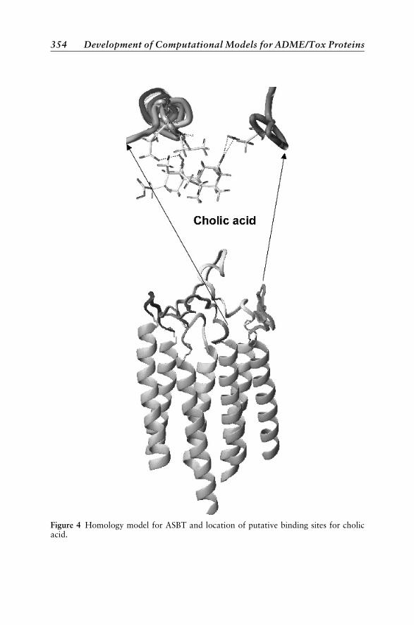
Figure 4 Homology model for ASBT and location of putative binding sites for cholicacid.


in reduced oral drug absorption and enhanced renal and biliary excretion ofsubstrate drugs. Moreover, P-gp expression at the blood–brain barrier is akey factor in the limited CNS entry of many drugs. The expressed level ofP-gp as well as altered functional activity of the protein due to genetic vari-ability in the MDR1 gene appears to also impact the ability of this transporterto influence the disposition of drug substrates.165

In terms of P-gp structure–activity relationship elucidation, photoaffinityexperiments have been valuable in defining the cyclosporin binding site inhamster P-gp166 and indicating that trimethoxybenzoylyohimbine (TMBY)and verapamil bind either to a single or to overlapping sites in a human leu-kemic cell line.167 Additional studies have shown that TMBY is a competitiveinhibitor of vinblastine binding to P-gp.168 The P-gp modulator LY 335979has been shown to competitively block vinblastine binding168 while vinblast-ine itself can competitively inhibit verapamil stimulation of P-gp-ATPase.167

With the growth in knowledge derived from these and other studies using dif-ferent probes and cell systems it would certainly be valuable to use structuralinformation to define whether unrelated molecules are likely to interact withP-gp. Early computational studies using P-gp modulators such as verapamil,reserpine, 18-epireserpine, and TMBY showed that these structures could bealigned suggesting the importance of aromatic rings and a basic nitrogen atomin P-gp modulation.169,170 A subsequent, more extensive study with 232phenothiazines and structurally related compounds indicated that moleculeswith a carbonyl group were active P-gp inhibitors.171 A model built with 21molecules of various structural classes that modulate P-gp ATPase activity sug-gested these molecules compete for a single binding site.172 Similarly, 19 pro-pafenone-type P-gp inhibitors were then used to confirm the requirement for acarbonyl oxygen that is proposed to form a hydrogen bond with P-gp.173

Klopman used MULTICASE to determine important substructural featureslike CH2��CH2��N��CH2��CH2,174 while Jurs used linear discriminant analysis

with topological descriptors175 in an attempt to model this property. In 1997,the first 3D-QSAR analysis of phenothiazines and related drugs known to beP-gp inhibitors was described.176 This was followed by Hansch-type QSARstudies using propafenone analogs,177,178 CoMFA studies of phenothiazinesand related drugs,179 CoMFA studies of propafenone analogues180 and simpleregression models of propafenone analogues.181,182 These latter models con-firmed the relevance of hydrogen-bond acceptors and the basic nitrogen forinhibitors181,182 and multiple hydrogen-bond donors in substrates being 2.5–4.6 A apart.183 One study utilizing a diverse array of inhibitors on P-gpATPase activity noted that size of the molecular surface, polarizability andhydrogen bonding had the largest impact on the ATPase activity.56 A numberof computational approaches and models of P-gp have yielded useful informa-tion that is usually derived from a series of structurally related molecules. Arecent experimental study suggested P-gp inhibitors with high lipophilicity


and polarizability are more likely to be high affinity ligands for the verapamilbinding site.184 A further example relied upon 2,4,5- and 2,3,4,5-substitutedimidazoles as P-gp inhibitors to derive similar CoMFA and CoMSIA modelsthat showed a sterically favored region around the phenyl substituent at theC-2 position of the imidazole ring.185

Interestingly, cytochrome P450 3A4 (CYP3A4), a drug metabolizingenzyme with a broad substrate specificity, appears to coexist with P-gp inorgans such as the intestine and liver. These observations lead to the hypoth-esis that there may be an interrelationship between these two proteins in thedrug disposition process. Wacher et al. described the overlapping substratespecificity and tissue distribution of CYP3A4186 and P-gp. Schuetz et al.187

found that modulators and substrates coordinate to up-regulate both proteinsin human cell lines. Similarly, P-gp mediated transport was found to be impor-tant in influencing the extent of CYP3A induction in the same cell lines as wellas in mice.187 More recent data suggest that there may be a dissociation ofinhibitory potencies for molecules against these proteins. Although somemolecules can interact with CYP3A4 and P-gp to a similar extent, for themost part the potency of inhibition for CYP3A4 did not predict the potencyof inhibition for P-gp, and vice versa.164 Moreover, not all CYP3A substratessuch as midazolam and nifedipine are P-gp substrates.188 Thus, although thereappears to be a relationship between the active sites of CYP3A4 and P-gp, thisrelationship is not by any means conclusive.

To account for the observed broad substrate specificities for bothCYP3A4 and P-gp, the presence of multiple drug binding sites has been pro-posed.189–192 The first experimentally determined signs of complex kineticbehavior for P-gp appeared in 1996 when cooperative, competitive, and non-competitive interactions between modulators were found to interact with atleast two binding sites in P-gp.193 The multiple site hypothesis was confirmedby other groups.194 –196 Subsequent results have indicated there may actuallybe three or more binding sites.197 Steady-state kinetic analyses of P-gpmediated ATPase activity using different substrates indicate these sites canshow mixed-type or noncompetitive inhibition indicative of overlapping sub-strate specificities.198 Other researchers have determined that immobilizedP-gp demonstrates competitive behavior between vinblastine and doxorubicin,cooperative allosteric interactions between cyclosporin and vinblastine orATP, and anticooperative allosteric interactions between ATP, vinblastineand verapamil.199 Clearly, allosteric behavior by multiple substrates, inhibi-tors or modulators of CYP3A4, or P-gp complicates predicting the behaviorand drug–drug interactions of new molecules in vivo. This has importantimplications for drug discovery. The computational modeling of P-gp hasbeen extensively reviewed recently,57 where it was suggested that althoughthere are many datasets available for modeling, combining those data maybe complicated by incompatibilities based on the assay and cell type used.Therefore our own modeling attempts have kept the data from different assays


separate so as to maintain this unique in vitro model-specific integrity and toallow for the production of computational models for specific, suggested bind-ing sites.

Recently, we have described how computational approaches can be usedto predict inhibition of P-gp by using in vitro data derived from structurallydiverse inhibitors of digoxin transport in Caco-2 cells, vinblastine, and calceinaccumulation in P-gp expressing LLC-PK1 (L-MDR1) cells or vinblastinebinding in vesicles derived from CEM/VLB100 cells.55 Using structurallydivergent P-gp inhibitors and probe P-gp substrates, we have been able togenerate distinct 3D-QSAR models that contain hydrogen-bond acceptors,hydrogen-bond donors, hydrophobes, and ring aromatic features. Some ofour models rank order the data in other data sets quite well, indicating partialoverlap for the binding sites probed by digoxin and vinblastine may exist.Models based on data for inhibition of vinblastine accumulation and vinblas-tine binding in different systems are not completely predictive for each other.Calcein accumulation data was not ranked to a statistically significant extentby either the vinblastine binding or the digoxin transport models. These differ-ent results may be indicative of some of the caveats associated with molecularmodeling of each respective system in vitro. The assays for accumulation ofsubstrates (vinblastine and calcein) involve inhibitors crossing the LLC-PK1cell membrane, and then presumably binding at unspecified sites within thecells. This is clearly mechanistically different, from inhibition of vinblastinebinding to plasma vesicles of CEM/VLB100 cells where the inhibitors onlyinterfere with binding. The data derived with calcein and LLC-PK1 cellsmay also indicate that we are dealing with binding to a separate site; however,the pharmacophore built with calcein data is able to rank the digoxin trans-port data, tentatively suggesting some degree of overlap of the pharmaco-phores. Overall vinblastine and calcein accumulation pharmacophores donot appear to be reliable for predicting the other P-gp data sets. This conclu-sion is based on the Spearman’s rho ranking statistic, the small energy differ-ence between null and final pharmacophores as well as the slight change in thisvalue following permutation. The lack of success with these two models maybe more a consequence of the limited structural diversity of the two trainingsets involved (large natural product structures), which in turn produce phar-macophores that explain less of the P-gp binding site(s) than from studies usingstructurally diverse training sets.

A Catalyst model constructed with 27 inhibitors of digoxin transport byP-gp appears to be the most useful and universal predictive model to date forboth molecules known to inhibit digoxin transport or vinblastine binding.55

This pharmacophore model contains one of the most potent inhibitors ofP-gp previously reported, namely, LY-335979 (IC50 0.059 mM,168), whichfits well to the model indicating that this may have potential for designingmolecules that fit this pharmacophore with similar or greater affinity. The vin-blastine inhibition pharmacophore was less predictive for the digoxin data as


judged by the model’s r2 value; however, the Spearman’s rho coefficient sug-gested that both models are equivalent (0.68 and 0.70) at ranking the com-pounds in the other training set. Taken individually, we may have definedpharmacophores for what could be interpreted as multiple regions withinthe same binding site of P-gp as probed by the particular substrates used inthe study. This hypothesis is based on each pharmacophore being slightly dif-ferent in its feature content, as well as its angles and distances. However, thesedifferences may actually be related to the structural diversity of moleculesin each training set or the use of IC50 values in most cases rather than dueto multiple-binding regions. This is a cautionary note, for novice and seasonedmodelers alike. Naturally, Ki values relate more closely to competitive inhibi-tors and a true binding affinity for P-gp and would be the ideal measure forgenerating such models. The cross-predictivity of most data sets in this studyprovide a means of model validation between IC50 and Ki data sets.55

The findings described above based on these different probes and cell sys-tems, is representative of similar computational studies commonly used inmany laboratories. Such studies serve as an initial step toward characterizationand prediction of P-gp-mediated drug transport both in vitro and in silico.From the above mentioned work, we hypothesized that vinblastine and digox-in are likely to bind to P-gp at a single site. This hypothesis was createdbecause strong correlations between the two models were observed. The utilityof the newly derived computational models was further tested using availableliterature data on verapamil-P-gp binding in vinblastine induced Caco-2cells.184 A new P-gp inhibition pharmacophore was constructed using thisverapamil-binding data and tested with the previously generated data.54 Ana-lyses of data using these computational models confirmed that verapamil mayinteract with the vinblastine–digoxin binding site(s) in P-gp. All four pre-viously generated pharmacophores for P-gp inhibition were useful in produ-cing statistically significant rank ordering of the verapamil-bindinginhibition data that was utilized in this second study. The Catalyst model(built with these 16 P-gp inhibitors of verapamil binding) was also predictiveas confirmed by the Spearmans rho value for the data generated in our pre-vious work that was based on inhibition of digoxin transport, vinblastinebinding, and vinblastine accumulation.

Our findings suggested that vinblastine, verapamil, and digoxin have anoverlapping affinity for similar or identical binding site(s) within P-gp. Thepresence of clearly defined regions in space occupied by clusters of identicalfeatures such as hydrophobes, hydrogen-bond acceptors, and ring aromaticfeatures was apparent by merging all five Catalyst P-gp inhibitor pharmaco-phores (Figure 5). To some extent, the inhibition pharmacophore for calceinaccumulation partially overlapped with the other four inhibition pharmaco-phores but its features did stand out. The initial P-gp pharmacophore, sug-gested by Pearce et al. in 1989169 as consisting of aromatic rings and a basicnitrogen atom, can be extended by the pharmacophores for P-gp inhibitors.


Using the digoxin transport model to predict 51 of the molecules from the vin-blastine binding, vinblastine accumulation, and verapamil accumulation datasets results in a correlation of observed versus predicted values (r2 ¼ 0:63) anda Spearmans rho ranking correlation coefficient of 0.75 (p ¼< 0:0001,Figure 6). This is quite acceptable as a computational model for drug discoverywhere large databases need to be filtered in a cost-effective manner.

Figure 5 Five merged P-gp inhibition Catalyst pharmacophores defining areas ofhydrophobicity¼ solid circles; aromatic rings¼ bold circle, and hydrogen-bondacceptors¼ square.

4

3

2

1

0

_1

_2

_3_1 0

log predicted IC50 (muM)

log

obse

rved

IC50

(m

uM)

1 2 3 4

Figure 6 Evaluation of the digoxin transport P-glycoprotein pharmacophore tested on51 molecules. Observed versus predicted IC50 r2 ¼ 0:63, Spearmans rho¼ 0.75,p < 0:0001, Elipse¼ 95% confidence interval.


The utility of the P-gp inhibitor pharmacophores produced to date wasalso assessed by using them to predict the rank order of other potential P-gpinhibitors not present in the data set used to create the models. A recent pub-lication presented data for the varying potency of P-gp inhibition of verapamilmetabolites.200 We utilized each pharmacophore model to predict the likelyIC50 of the four verapamil metabolites D-617, D-620, D-703, and norverapa-mil. All five pharmacophores were able to identify the least potent P-gp inhi-bitors correctly as being D-617 and D-620. These molecules are more likely tobe hydrophilic as suggested previously for other low-affinity binding inhibitorsat the verapamil site.184 Two of the pharmacophores that are based on inhibi-tors of digoxin and verapamil binding provided useful quantitative predictionsfor the inhibition of verapamil transport with verapamil metabolites. Thedigoxin pharmacophore performed particularly well with the potent inhibitorsD-703 and norverapamil because these molecules fit the majority of the fea-tures in the models. The third model, based on inhibitors of vinblastine bind-ing, failed with D-703 (the prediction exceeded 1 log order of magnitude).These predictions for verapamil metabolites are perhaps not totally unex-pected because all three of these models used verapamil as a training set mem-ber. However, the digoxin model used a much higher IC50 value for verapamilthat makes it one of the least potent inhibitors. This in turn might explain itslower predicted value in this case. Our models for inhibition of vinblastine andcalcein accumulation differed from one another in that the latter model wasless quantitative in the nature of the predictions even though it could generatethe correct rank order for the verapamil metabolites. Once again this lack ofquantitative agreement may be a function of the complexity of the systemrequiring absorption prior to the inhibition that is measured. Future studiesincorporating additional P-gp probes may define new binding sites or aid inthe generation of more detailed pharmacophores that could prove valuablefor both drug discovery and screening. Molecular-modeling studies like thishave the potential to enhance our understanding of complex transporterssuch as P-gp without having a crystal structure, and such studies may beapplied to other systems as well.

The hypothesis that some of the substrate probes for P-gp bind to similarsites was tested further. By alignment of verapamil and digoxin followed byfitting vinblastine, it was possible to identify possible common features acrossall three substrates. All three molecules have extended conformations withhydrophobic and hydrogen-bond acceptor features in common. These featuresare distributed toward the extremities of the molecules. This P-gp substratepharmacophore therefore appears to be consistent with the features presentin some of the inhibitor pharmacophores generated previously.54,55 The align-ment of other known P-gp modulators such as TMBY and reserpine was eval-uated with this P-gp substrate model derived from the verapamil and digoxinalignment. Both TMBY and reserpine molecules could be fit to multiple fea-tures of the pharmacophore in the extended conformations and reserpine


was also fitted to similar pharmacophore features as verapamil. This finding isonce again in agreement with previous work in which the reserpine analogueswere aligned using different software169 and provided additional supportfor our suggestion that vinblastine, verapamil and digoxin are likely to bindto similar sites in P-gp. Our findings are also consistent with available in vitrodata for binding of substrates.167,168 These recent in vitro and in silicoapproaches appear to confirm the chemical features deemed to be importantfor binding to this site as either substrates or as inhibitors. A recent pharma-cophore model for P-gp substrates based on 144 molecules, generated 3 millionpharmacophores (using in-house software).58 Of those pharmacophores, anensemble of 100 was used for predictions.58 A threshold of 20 pharmaco-phores was set such that molecules matching less than this number wouldbe indicated as nonsubstrates. This model correctly classified 80% of the train-ing set but only 63% of the test set.58 The pharmacophores used containedhydrogen-bond donors, hydrophobic, and aromatic ring features, but thehydrogen-bond acceptor was felt to be the most important feature. The utilityof this model may be limited by its relatively poor predictivity, however,improvements could be made by increasing the amount of training data.Further pharmacophore-based approaches201 using GASP alignments to vin-blastine and to rhodamine 123 have been carried out to understand the vera-pamil binding site.201 Those studies revealed similar pharmacophorerequirements as proposed earlier. Multiple hydrophobic and hydrogen-bonding interactions were described.201 A small number of P-gp ligandswere superimposed with SYBYL and MOLCAD by Garrigues et al.202 togenerate two pharmacophores. The resulting models were validated withonly two additional compounds, however. The generation of data for P-gpin other species including rat and mouse203 will aid in our understanding ofthe binding sites of this transporter.

When the P-gp pharmacophores in previous studies54,55 are comparedwith pharmacophores for inhibitors and substrates of CYP3A97,204 (Figure 7),some similarity is found between them.54,55 Both P-gp and CYP3A share phar-macophores with multiple hydrophobic features and at least one hydrogen-bond acceptor feature albeit in slightly different arrangements. This mightexplain why potent CYP3A4 inhibitors are not necessarily potent P-gp inhibi-tors164 or substrates.188 This slightly different arrangement helps clarify theindependent nature of the relationship between ligands that bind to thesetwo proteins.

Vitamin Transporters

The ascorbate transporter SVCT1 has been shown to be inhibited bysome flavonols such as quercetin but less so by the related catechins.205 Theabsence of the ketone at the 4-position of the C ring has a dramatic negativeeffect on the potency of inhibition, suggesting that a key hydrogen-bonding


interaction is required for maximal inhibition. The addition of a glycone groupon the C ring also affects inhibition suggesting that the transporter has somesize limitation. Quercetin is a noncompetitive inhibitor of SVCT1 as well asthe glucose transporter GLUT2.205 No QSAR has been generated to ourknowledge for the SVCT1 or GLUT2 transporter for either substrates or inhi-bitors to date. Development of a QSAR may be valuable for prodrug design asa viable means to improve membrane penetration of some drugs by addition ofan ascorbic acid mimic.206

Organic Cation Transporter

The organic cation transporter, OCT1, is likely to play a role in the hepa-tic elimination of many cationic drugs.207 A number of studies have describednew molecules that interact with OCTs.208,209 Understanding the 3D featuresfundamental to molecular interaction with the transporter would thus bevaluable. Hydrophobicity and basicity may be important substrate require-ments for interaction with the OC transporters on the apical and basolateralmembranes of the rat renal proximal tubule210 and on the apical and baso-lateral transporters in rabbit.211–213 Structure–activity relationships havebeen developed for substrates of the OCþ/Hþ exchanger.212 The binding siteof the luminal transport step of rabbit renal proximal tubules, the OCþ/Hþ

exchanger, includes a planar hydrophobic surface that is sufficiently accom-

modating so that no steric exclusion is evident when a planar (9� 12A) hydro-phobic mass is rotated about an N-pyridinium center. A more recent studywith OCT1 used a number of structurally diverse ligands to derive QSARmodels with ClogP alone or with multiple descriptors in Cerius2 and a phar-macophore model with Catalyst.214 Future detailed computational studiesundoubtedly will be required for both human OCT1 and OCT2 to understandtheir individual specificities.

Figure 7 The partial similarities between a substrate pharmacophore for CYP3A4 (a), aCYP3A4 autoactivator pharmacophore (b), and a CYP3A4 inhibition pharmacophore(c). Legend: H¼ hydrophobe; HBA¼ hydrogen-bond acceptor; HBD¼ hydrogen-bonddonor.


Organic Anion Transporters

The rat kidney organic anion transporter (OAT) is characterized by itstransport of p-aminohippurate, cAMP, and cGMP and by its inhibition by var-ious anionic drugs. Although there have been many studies with rat OATsshowing inhibition with beta-lactam antibiotics215 and with other drugs, therehave been no QSAR studies. A comprehensive review of transporters involvedin organic anion transport208 indicates there is little published on the topic ofligands for the human OATs. However, a recent study described the interac-tions of 12 NSAIDS with hOAT1, hOAT2, hOAT3, and hOAT4.216 BothhOAT1 and hOAT3 demonstrated higher affinity binding with NSAIDS. Itwas suggested that this high affinity may explain some adverse physiologicalreactions. This small dataset might provide a viable starting point for apharmacophore analysis of these transporters that in turn could be used forcomparison with the hOCT pharmacophores generated to date.

Nucleoside Transporter

Nucleoside transporters (NTs) are important in mediating transport ofnucleosides and nucleoside drugs (e.g., antiviral and anticancer drugs) acrosscell membranes.217 These transporters can be classified into two broad cate-gories: the Naþ-dependent concentrative (energy-dependent) transporters,which physiologically mediate influx of nucleosides, and the Naþ-independentequilibrative (or facilitative) transporters, which mediate both influx andefflux. Five principal Naþ-dependent concentrative nucleoside transporters(CNTs) have been identified so far. Of these, only two CNTs, CNT1 andCNT2, are found to be functionally present in the epithelial cells of organsimportant for drug absorption (intestine) and elimination (kidneys). BothCNT1 and CNT2 transport uridine and adenosine218 and are insensitive toinhibition by nitrobenzylthioinosine (NBMPR). The equilibrative transportersmediate both the influx and efflux of nucleosides and exhibit broad substratespecificity, accepting both purine and pyrimidine nucleosides as permeants.Equilibrative nucleoside transporter 1 (ENT1, es) is inhibited by NBMPR con-centrations as low as 0.1 nM (IC50 �0.4 nM), whereas the ENT2 (ei) trans-porter is insensitive to inhibition as high as 1 mM (IC50 �2.8 mM).217 TheENT1 transporter is expressed in most, if not all, cell types while ENT2 isselectively expressed in some tissues such as muscles. By using a chimerictransporter T8 containing the rat N1 and N2 transporters, it was suggestedthat purine and pyrimidine nucleosides share a common binding site.219 Astructural inhibitory profile for the N1 and N2 transporters in human intes-tinal brush border membrane vesicles was produced using two concentrationsof anticancer and antiviral drug analogues.220 It was found that the 30-oxygenin the ribose ring is required for inhibition. Further, the N2 transportercan tolerate substitution at the 50-position, whereas the N1 transporter ismore sensitive to substituents. The ribose or 20-deoxyribose is necessary for


high-affinity interaction with both transporters. The 6 and 8 position on uraciland adenosine, respectively, are critical for inhibition of N1 and N2 transpor-ters.220

Our laboratory has compared the relative and the unified structuralrequirements of nucleosides for high-affinity interaction with hCNT1,hCNT2, and hENT1.221 By using nucleoside transporter inhibition datafrom a series of uridine and adenosine analogues (and a variety of nucleosidedrugs),219,220 a unique pharmacophore model for each transporter was gener-ated with DISCO. Two multivariate regression analyses, CoMFA and GOLPE,were used to generate QSAR models that correlate substrate–inhibitor struc-tural features with their binding affinities. The overall qualities of the resultingmodels were then used to construct more comprehensive models. It was foundthat both the hydrogen-bond acceptor and donor surrounding the 30 carbon isrequired for hENT1 substrates. It was also found that a hydrogen-bond accep-tor on the ribose next to the pentose ring is important for hCNT2 substrates,whereas hydrogen-bonding at the 50 carbon is important for hCNT1 affinity.The CoMFA and (GOLPE) QSAR models with cross-validated r2 values of0.52 (0.69), 0.65 (0.69), 0.74 (0.70) were derived for hCNT1, hCNT2, andhENT1, respectively. The hCNT1 QSAR model displayed mainly hydrogen-bonding features, whereas hCNT2 and hENT1 exhibited electrostatic andsteric features. Quantitative results correlated well with experimental analyses,suggesting subtle and unique structure–activity correlation for each nucleosidetransporter. These QSAR models should now allow for the design of high-affinity nucleoside transporter inhibitors and substrates for both anticancerand antiviral therapy.

Breast Cancer Resistance Protein

The identification of a new ABC transporter termed the breast cancerresistance protein (BCRP, MXR, ABCG2) has revealed that increased expres-sion of this transporter results in resistance to anticancer therapeutics. Therecent suggestion that this transporter is also expressed in the intestine suggeststhat this transporter could also be important in limiting bioavailability andthat Caco-2 cells express this at the level seen in the jejunum.222 Understand-ing early in discovery how other drugs, and in particular new anticanceragents, are readily transported by this protein is important. To date, there arelimited SAR type studies from which to initiate computational modeling. Infact, there exists only one with a large number of molecules, consisting of42 diastereoisomeric mixtures of fumitremorgin-type indoyl diketopiperazineinhibitors of BCRP.223 A further study focusing on the topoisomerase Idrugs has described the affinity for BCRP (in decreasing order) as SN-38 >topotecan > 9-aminocamptothecin > CPT-11 > NX211 > DX8951f >BNP1350.224 Future studies analogous to those with P-gp will be necessaryin order to generate more generally predictive computational models for BCRP.


Sodium Taurocholate Transporting Polypeptide

The transport of bile acids in the liver occurs via the sodium taurocholatetransporting polypeptide (NTCP). Alterations in this activity contribute tocholestasis. A recent evaluation of 33 molecules (including commonly useddrugs) to assess drug-induced cholestasis found that besides bile acids, propra-nolol, progesterone, cyclosporine, and a number of oligopeptides are potentinhibitors of taurocholate uptake.225 Eight of these molecules demonstratedan IC50 between 1 and 264 mM and recently have been used to generatea pharmacophore that consists of two hydrophobic features and twohydrogen-bond donor features226 (Figure 8). Interestingly, it has also beenreported that class I antiarrhythmics can enhance bile acid uptake via thistransporter, which to date has not been studied in detail.225 A more completeQSAR analysis for this transporter is required in the future.

ENZYMES

Cytochrome P450

Since their discovery as heme thiolate proteins in the late-1950s, thecytochrome P450s have been recognized as the largest family of enzymes

Figure 8 A pharmacophore for the human hepatic sodium-dependent bile acidtransporter using eight molecules and IC50 values demonstrating two hydrophobicfeatures (bottom right) and two hydrogen-bond donors (top left and top right). Theobserved versus predicted data resulted in a correlation r ¼ 0:97. A training set member(ursodeoxycholic acid) is shown fitted to this pharmacophore.

Enzymes 365

known to be present across all organisms with CYP51 being present in everyphyla.6 The cytochrome P450 enzymes are considered by some to be the mostimportant enzyme family in terms of endobiotic and xenobiotic metabolismbecause of their ubiquity and because they are expressed within many tissuessuch as the liver and intestine. By the 1970s, this superfamily started to grow,and through the 1980s–1990s many of them were purified, cloned, orexpressed in other cell systems that allowed for a great deal of characterizationand understanding of the requirements needed for substrate and inhibitoraction. Some cytochrome members are human enzymes (families 1, 2, and3) that were thought to be important for xenobiotic metabolism, and thereforewere more widely studied than others. The use of in vitro systems to elucidatepotential drug–drug interactions (DDI) became readily adopted by drug com-panies and the FDA. The cost of this research focus was offset by the lack ofstudy of other enzymes, especially those outside of the CYPs involved in con-jugative metabolism.

Unfavorable DDIs are clearly important and clinically relevant.227 Eventhough in some populations the number of DDIs may seem small, they are animportant factor in determining whether or not a new chemical entity will suc-cessfully make it beyond a drug discovery program to development. In addi-tion, the late discovery of a clinically significant DDI could be costly in termsof the financial investment of a particular project. Therefore it is important toscreen for potential interactions228 early on, to aid in the selection of the mostappropriate in vivo studies.229,230 In this regard, drug interactions with cyto-chrome P450s (CYPs) are particularly important,231 but ultimately avoidable(depending on the therapeutic index), even though drug metabolism is com-plex and to some extent predictable by careful assessment of structure–activityrelationships. The enzymes CYP1A2, CYP2C9, CYP2C19, CYP2D6, andCYP3A4 represent > 90% of total hepatic P450232 and nearly 80% of thera-peutic drugs are metabolized by these same enzymes.233 Interaction with oneor more of these enzymes in vivo would thus pose a potentially relevant event,clinically. In recent years, in vitro systems have proved invaluable in predictingthe likelihood of DDI231 because they allow identification of the CYPs respon-sible for metabolism as well as determination of the relative contribution tooverall elimination of the inhibited pathways.234 Because the number of mole-cules synthesized by pharmaceutical companies has increased dramaticallywith the utilization of combinatorial chemistry, there is now a shift in empha-sis toward earlier implementation of higher throughput in vitro studies formetabolism235,236 or lead optimization.237

The CYPs may be involved in many DDIs because of their affinity forhydrophobic molecules of varying sizes. It is widely believed that an under-standing of DDIs at the molecular level may lead to the development ofmore effective and safer therapeutics. In the absence of a freely availablecrystal structure for any of the human CYPs, there is an obvious need tobuild computational models in an attempt to predict drug metabolism and


interactions prospectively. Many approaches have been taken using varioustools in this regard. Comprehensive analysis of existing physicochemicaldata, protein homology data, nuclear magnetic resonance (NMR) data, sitedirected mutagenesis results and insights from QSAR approaches have allbeen used. Recent reviews have described and compared the many pharmaco-phores for CYPs.24,238 The foundation for those types of studies were laid inthe late-1960s by Hansch et al. using mathematical approaches that includelipophilic character to describe metabolic characteristics of drugs. In the inter-vening years, there was a great emphasis on developing in vitro approaches formetabolism such that we are now aware that there exist many human CYPs ofimportance. The distribution of these enzymes, their expression in various tis-sues and the extent to which they metabolize commercially available drugs hasalso been widely studied. A major advance in technology for in vitro studies ondrug-metabolizing enzymes involves the availability of recombinant enzymesboth for CYPs and phase II enzymes. These recombinant CYPs have enabledthe development of high throughput screens for DDIs and, concurrently, haveprovided increasingly large databases of molecules for computational model-ing. This reductionist perspective may be problematic because removing mole-cules early in drug discovery based upon their poor performance in thesescreens may not account for molecules that may be dosed at significantly lowerconcentrations than usually assessed for CYP inhibition. Initially, 3D-QSARmodels were built with CYP data derived from human liver microsomaldata using a substrate probe shown to be relatively selective for the enzymein question. This is likely not to be as clean a system as using the purifiedenzyme, hence models derived from such data are less desirable.

CoMFA models were first used with CYP1A2,239 CYP2A5,240 andCYP2C9,241 using relevant conformers of inhibitors to suggest key functionalgroups, the geometry of selected structural features, and regions of electro-static and steric interactions. Those studies typically used data from humanliver microsomes and a probe substrate. More recently, QSAR models havebeen built after analysis of literature data including recombinant-derivedkinetic values for enzymes such as CYP2B6,100,242 CYP2C9,241,243 andCYP2D6.244 There have been a number of groups that have combined phar-macophores with homology models of either bacterial CYPs241,245–247 or therecently crystallized rabbit CYP2C5/3.242–244,248 One study generated ahomology model of CYP2B6 based on CYP2C5 (48% sequence identity)and also modeled the missing F and G helices by unconstrained moleculardynamics.249 This study249 and others242,250 have shown the importance ofhydrophobic interactions with substrates using homology modeling that hadalso previously been suggested by a pharmacophore.100 Because the CYP phar-macophores have been described previously, the reader is referred to the pri-mary literature cited.

Members of the CYP3A family of enzymes are the most importantin terms of human drug metabolism,251 because they have wide substrate

Enzymes 367

specificity and are inducible by structurally unrelated compounds.252 At pre-sent, we are aware of four differentially regulated CYP3A genes in humans:CYP3A4, CYP3A5, CYP3A7, and CYP3A43. The CYP3A4 gene is dominantin terms of hepatic expression and is inducible.251 The CYP3A5 gene is poly-morphically expressed in the liver and may constitute as much as 50% ofhepatic CYP3A in a third of Caucasions and one-half of African Americanswithin the population.253 The CYP3A7 gene is the fetal form of CYP3A andis believed to be of low abundance in adult liver251 while CYP3A43 is newlyidentified with, at present, little understanding of its expression and catalyticactivities.254 One enzyme in particular, CYP3A4, has drawn considerableattention over the past decade because it metabolizes a large percentage ofthe molecules that are substrates for the CYPs.251 Computational modelingof ligands for this enzyme has defined hydrogen bonding and hydrophobicityas important determinants of substrates.204 (Figure 7). While computationalinhibitor models of CYP3A4 differ slightly (depending on the substrate probeused in vitro) they maintain the trend of highlighting hydrophobic and hydro-gen-bonding features.97 More recently, there has been a focus on studying theregulation of human CYP3A with the intent to understand the expression ofthis enzyme and the variability in bioavailability and clearance of its substratesacross the population253 as well as for understanding drug–drug interac-tions.255,256 One of the few early QSAR studies of inducers of CYPs basedon in vitro and in vivo data assessed the rat CYP3A family and describedthe electrostatic potential maps for 16-substituted pregnenolones. From thatQSAR, it was suggested that the length of the 16a substituent is related tothe in vivo and in vitro induction while the steroidal skeleton of these mole-cules is involved in lipophilic (hydrophobic) interactions.257 A QSAR studywith 14 steroid inducers of rat CYP3A showed that the difference betweenfrontier orbital energies, �E, correlated well with biological activity.258 Theauthors also suggested that hydrogen bonding and hydrophobic interactionswould be important in the receptors involved in induction. It was several yearsbefore we were able to predict induction of human CYP3A4, and it took thediscovery of a new nuclear hormone receptor to catalyze that development(described later in this chapter as the pregnane X receptor).

Assessment of the inhibitory potency of CYP3A enzymes is oftenincluded as a first tier screen in early drug discovery alongside CYP2D6. Fluor-escent probe substrates are now widely used for this screening purpose andoffer the advantages over conventional compounds of being amenable tohigh throughput and being capable of real-time analysis.259,260 Data fromsuch front-line screening tests is often supplemented with that from traditionalsubstrate probes.261 The interaction between CYPs and their substrates in vitrois complex, as exemplified by CYP3A4.189,190 Incubation buffer constituentsappear to be able to alter the behavior of the enzyme262 in addition to the con-formation of the CYP3A4 active site.263 Furthermore, inhibition of theCYP3A4 catalysis is substrate dependent.259,264,265 In a study of CYP3A4


inhibition utilizing 10 substrates and 34 inhibitors, it was shown that CYP3A4substrates could be clustered into more than three groups according to theeffects of the inhibitors.265 Data from various studies are consistent withthe active site of CYP3A4 simultaneously accommodating two or more sub-strate molecules.190,266,267 Kinetic models have been proposed for two sub-strate molecules binding simultaneously to the CYP3A4 active site.190,268

Updated kinetic models for the interaction of these multiple molecules in thebinding domains within the active site have also been developed.269 Midazo-lam has been used to covalently modify a site occupied by triazolam inCYP3A4, in preference to a site occupied by testosterone.270 Experimentalevidence derived from substitution of substrate recognition residues in theCYP3A4 active site suggests that there exist two substrate-binding subpocketsand one ‘‘effector–binding’’ region266 similar to previous suggestions of ahydrophobic domain that is considered as being important for activa-tion.204,271

An alternative hypothesis for the observations of substrate-dependentinhibition of CYP3A4 activity is that the enzyme exists in multiple conforma-tions.272 Another theoretical model proposes the concept of ‘‘nested allosterism’’,where multiple conformations of the enzyme exist both in the presence andabsence of substrate, and where each conformer is sensitive to allostericeffects.273 Mathematical and computational models have generated some use-ful information on ligand binding for CYP3A substrates204 and CYP3A4 inhi-bitors.97,274 Pharmacophore models in particular have offered the advantageof providing an interpretable visual representation of the structural featuresof compounds important for binding to CYPs as well as being able to providea reasonably predictive model.22,24 These models are unified in suggesting theimportance of hydrophobicity for CYP3A4 substrates.

Because members of the CYP3A family of enzymes are the most impor-tant in terms of human drug metabolism,251 have wide substrate specificities,and are inducible by structurally unrelated compounds,252 it is of value tounderstand some of the important features of ligands that bind to theseenzymes. Previously, we showed the utility of generating computational phar-macophores for CYP3A4 substrates204 and inhibitors97 using Ki (apparent) andIC50 data (as summarized with other CYP pharmacophores,24 Figure 7). Thisapproach was also used to determine the important features of autoactivatorsof CYP3A4 that possess three hydrophobic features and one hydrogen-bondacceptor204 (Figure 7b). This finding seems to agree well with site-directedmutagenesis data from another group.271 A neural network has been applied inan attempt to differentiate between substrates and inhibitors of CYP3A4. Inthat study, literature data was collated from the human P450 metabolismdatabase.275 The model derived from that neural network was used to predictpreviously published data on structurally diverse CYP3A4 inhibitors,97 butthe model did not rank correctly the Ki data. The inhibitor LY024410(Ki 701 mM) had the same score as most of the other molecules (Ki range

Enzymes 369

1.8 – 492.7 mM), while LY213829 was misclassified as a noninhibitor (Ki 6.6mM). It remains to be seen whether such a wide classification of inhibitors isuseful for drug discovery screening. The recent crystallization of CYP3A4 byresearchers at Astex now presents an opportunity to validate all of the avail-able computational models to date and to discern how activators and autoac-tivators behave in the active site of that protein. It is hoped that crystalstructures for CYP3A5 and CYP3A7 will become available in the nearfuture because such structures could provide some additional insight intothe endogenous and developmental role of all of the members of the CYP3Afamily.

Epoxide Hydrolase

The epoxide hydrolases are known to catalyze the hydrolysis of epoxidesor arene oxides to diols by addition of a water molecule. This process isthought to be a two-step process involving the formation and hydrolysis ofa covalent acyl- or alkyl-enzyme intermediate. Both microsomal and solubleforms of the enzyme possess activity toward toxic xenobiotic epoxides. Thesoluble epoxide hydrolase (sEH) has an endogenous role in the hydrolysis ofthe epoxides of arachidonic and linoleic acid, known regulators of vascularpermeability. The potential for therapeutic utility has been explored by gener-ating numerous inhibitors of sEH. Several studies have generated QSAR mod-els for sEH. A QSAR using Hansch substituents for 27 chalcone oxideinhibitors of mouse sEH suggested that steric and electronic features areimportant mediators of inhibition.276 Human data with the same moleculesproduced a weaker correlation.276 A CoMFA analysis of murine sEH inhibi-tors by molecules like benzoylureas, arylureas, and other analogues was per-formed using 37 molecules.277 Large sterically unfavorable fields were foundabove the A ring and the urea bridge of benzoyl-phenylureas, while stericallyfavorable areas were found below the A and B rings of the 37 molecules ana-lyzed. In addition, a number of negative electrostatic potential fields were pre-sent around the whole molecule along with a positively charged area beneaththe carbonyl carbon atom that is important for activity.277 These computa-tional models complement the murine X-ray crystallographic data and sitedirected mutagenesis studies confirming key roles for Tyr465 and Tyr381 ashydrogen-bond donors to the urea carbonyl group and that Asp333 is involvedin the nucleophillic attack.278,279 Crystallization of the human sEH enzymewill be of value in the future to test QSAR models generated with human inhi-bitors. This in turn will allow us to predict the likelihood of epoxide hydrolysisfor other xenobiotics that may not be as desirable.

Monoamine Oxidase

The monoamine oxidases are present in the outer membrane ofmitochondria and are known to catalyze oxidation of many important


neurotransmitters. Monoamine oxidase A (MAO-A) inhibitors are valuableantidepressants and antianxiety molecules while monoamine oxidase B(MAO-B) inhibitors have found use in treating Alzheimers and Parkinsons dis-ease. Consequently, there has been considerable interest in developing reversi-ble inhibitors of these enzymes.280 Besides their importance in the CNS as atherapeutic target, these enzymes are expressed in the liver (to some extent)and they may have a role in the metabolism of xenobiotics thus providingan opportunity for DDI.281 Structure–activity data have been generated witheither the rat brain282 or rat liver283 mitochondrial preparations for only a nar-row chemical series to date. A study of 16 pirlindole inhibitors (IC50) withMAO-A and MAO-B showed that most inhibitors were more potent againstMAO-A. A CoMFA analysis used subsets of these molecules and indicatedthat the active site of MAO-A can accommodate long rigid molecules. Contra-rily, with MAO-B, flexible and more hydrophobic molecules are preferred.283

For a series of 19 condensed pyridazines and pyrimidines (IC50 values gener-ated with MAO-B), a QSAR analysis using Hansch, electronic constants,enthalpic, and entropic contributions as well as volume descriptors alsoshowed hydrophobicity being the most important parameter relating to inhi-bitor binding.282 A CoMFA analysis based on 16 indolylmethylamine deriva-tives (Ki data is available for both MAO-A and MAO-B) showed there existsimilar contributions from steric, electrostatic, and solvation terms for MAO-A and MAO-B and that the indole ring appears to act with different electro-static responses toward each enzyme.284 A large series of coumarin derivativeshas also been evaluated and their IC50 values were used for deriving Hansch-type QSAR and CoMFA/GOLPE models with 41 and 44 molecules for MAO-A and MAO-B, respectively. Only the electrostatic field was able to explain theMAO-A data. Better statistics were derived for the MAO-B model using steric,electrostatic, and hydrophobic fields.285 In general, the findings of this latterstudy are in agreement with those described previously by others, wherehydrophobicity was found to be a factor leading to increased selectivity forMAO-B while the presence of a sulfonic ester at the 7-position of the moleculeincreased MAO-A activity.285 A further study has relied upon Catalyst tocorrelate MAO inhibition with structure for five molecules.286 The model con-tained a carbamate group, an aromatic hydrophobe, a hydrogen-bond donor–acceptor and a hydrogen-bond donor. When fitted to experimental bindingdata it suggested that 6-carbamoyl-N-propargylaminoindans are less potentthan 6-carbamoylaminoindans.286 The appearance of large diverse humanMAO-A and MAO-B data sets in the literature appears to be some way offin the future. For now, models for the human enzymes will have to assumethere is some similarity to the rat enzymes. The few examples where humanenzyme have been used involve MAO-A. Structure–activity relationships(based on Kd values) have been generated for phenethylamines and benzyl-amines. The rate of substrate oxidation correlates best with electronic substi-tuent effects for para substituted benzylamines,287 while the Taft steric value

Enzymes 371

for alkyl side chains was found to be related linearly to the observed bindingaffinity.288

Flavin-Containing Monooxygenase

The flavin-containing monooxygenases FMOs are important in theN-oxidation of nucleophiles.289 Few quantitative studies suitable for derivinga QSAR have been performed on this enzyme family, although one researchgroup has suggested (after using a size analysis and in vitro Km determination)that human FMO1, which is known to metabolize imipramine and orphena-drine, can also metabolize methimazole, thoiurea, and phenylthiourea, but not1,3-diphenylthiourea. This and other members of the FMO superfamily maybenefit from future QSAR studies once sufficient data is generated.

Sulfotransferases

The formation of sulfate conjugates of both endogenous and exogenousmolecules occurs via the cytosolic enzyme sulfotransferase superfamily utiliz-ing phosphoadenosine phosphosulfate (PAPS) as the donor. There may be 10or more of these enzymes in humans one of which (SULT1A3) is expressed inthe intestine and is important for the sulfation of amine neurotransmitters,drugs, and other xenobiotics. This enzyme was recently crystallized andexperimental Km data was used to derive a QSAR.290 This stepwise regressionQSAR suggested that hydrogen bonding and hydrophobicity are important forbinding to the enzyme, which is consistent with the crystal structure that con-tains three hydrophobic phenylalanine residues creating a hydrophobic site.The expression of SULT1A3 in the breast and the potential for this enzymeto metabolically activate promutagenic derivatives of heterocyclic amines,291

suggests that computational models of this or other related enzymes may alsobe useful.

Considerable amounts of Km data have been generated for the rat hepaticaryl sulfotransferase (AST IV) that has a broad substrate specificity. These dataprovide some understanding of the influence of substrate structure and stereo-specificity on catalysis.292 One research group has also analyzed the kinetics ofsulfation for primary293 and secondary294 alcohols, 1-aryl ethanols,295 andN-alkyl-N-hydroxyanilines.296 These data, in total, present a valuable startingpoint for QSAR analysis of this enzyme. It is presumed that hydrophobicityand steric effects play a large role in determining the specificity because thereare clear limits to the size of molecules that can act as substrates.293 Homologymodeling has also played a role in interpreting binding of inhibitors as well assubstrates and their proximity to PAPS.296 A recent CoMFA and homologymodeling study used 35 molecules as the training set and a six molecule testset, which were combined to predict Kcat/Km.297 Perhaps we can use the rat


data and use computational models for this and other rat sulfotransferases toeventually aid in predictions for human sulfotransferases.

Glucuronosyltransferases

Glucuronidation of small lipophillic molecules is an important metabolicprocess for the clearance of drugs, endobiotics and xenobiotics in all mamma-lian species.298 In numerous instances, drugs azidothymidine (AZT), valproicacid, propofol, morphine, and others) are cleared extensively by direct glucur-onidation,299 although in many other cases the involvement of glucuronida-tion is restricted to the conjugation of glucuronic acid to metabolites ofphase I oxidative metabolism. In cases where drugs are significantly glucuro-nidated independently of phase I metabolism, the functional group to whichthe glucuronic acid is transferred can be a hydroxyl group (phenolic or alipha-tic), a carboxylic acid, or in some cases an amino group (primary, secondary,or tertiary).

The uridine diphospho-glucuronosyltransferases (UGT) family can beseparated into two distinct subfamilies by sequence similarity. The UGT1and UGT2 family of isoforms are known to be encoded by individual genes.300

Characterization of cloned and expressed human UGT has demonstrated thatmany UGT family 1 isoforms are capable of glucuronidating phenols to vary-ing degrees including UGT1A1,301 UGT1A3,302 UGT1A4,303 UGT1A8, andUGT1A10.304 The UGT family 2 isoforms also display activity toward phe-nols, although substrate acceptance and rate of glucuronidation appears tobe more restricted for UGT2B15305 and UGT2B7.306 Two of the earliestUGT isoforms examined were done so on the basis of their ability to glucur-onidate phenols. Both UGT1A6 and UGT1A9 were classified as phenol UGTisoforms due to the high turnover rates of these substrates.307 The UGT1A9demonstrated greater proficiency in glucuronidating bulky and complex phe-nols than UGT1A6, which was considered to be capable of glucuronidatingonly simple or planar phenols.307 The high glucuronidation activity towardsimple phenolic substrates has been shown to be present in human liver micro-somes308 and UGT1A6 comprises a significant proportion of liver UGT1-naphthol glucuronidation capacity.309

Phenols have also been used as probe substrates for simple structure–activity relationship modeling, but very few reports of glucuronidation QSARshave been reported. Enzyme activity data sets for phenols and for benzoicacids incubated with rabbit and rat liver microsomes (published before UGTheterogeneity was recognized) have subsequently been used for QSAR model-ing.80,310,311 Since those original reports, much of the data contained withinhas been reanalyzed.312 Kinetic constants for simple phenolic substrateglucuronidation were modeled by QSAR to characterize a partially purifiedrat UGT.313 Using rat microsomal systems for this type of work furthercomplicates any modeling of a heterogenous population of enzymes that can

Enzymes 373

display a considerable overlap in substrate specificity for different types of sim-ple compounds. By accounting for these problematic assumptions, it seemslikely that models derived from rat microsomes are limited in the informationthey provide. The generation of a QSAR for inhibitors in vitro and substratesin vivo has afforded us some degree of understanding of the rat UDPGT.314,315

The benefit of studying isolated enzymes is that complications introduced bytrying to predict the glucuronidation activities of a heterogenous population ofisoforms are avoided, and, the substrate physicochemical parameters can berelated directly to their influence on activity and affinity of a single active site.

A more recent study described the glucuronidation of simple 4-substi-tuted phenols by the human UGT1A6 and UGT1A9 isoenzymes.316 The

Cerius2 genetic function approximation software was used to produce modelsfor these isoenzymes. Models to determine whether the Km for phenol glucur-onidation could be predicted were generated for UGT1A6 and UGT1A9 usinga range of molecular surface (MS-WHIM) and atomic (AT-WHIM) descrip-tors. The models were used to compare the way these two isoforms glucuro-nidate phenols. These models were also used to determine the viability ofdeveloping QSAR models for more complex and diverse substrates in thefuture.

Although the molecules that were screened by testing with both isoformsvary only in the substituent at the 4-position, this position seems to be an espe-cially important factor in determining whether a compound is or is not a sub-strate of UGT1A6. Again, UGT1A9 was shown to be proficient atglucuronidating a wide range of substituted phenols as reported previously.307

This is the first indication of significant differences between the two isoforms.By comparing the Km values for the set of phenol substrates that are glucuro-nidated by both isoforms, one finds substantially lower Km values for UGT1A9than for UGT1A6 even though the ranges of Vmax are similar. Another point ofinterest is the observed trend between UGT1A6 Vmax and the molecularvolume of substrates. Even without the application of QSAR analysis it wasclear that UGT1A6 Vmax values decrease as the bulk of the para-substituentincreases.

Glucuronidation of 19 indolocarbazoles in human liver microsomes wascarried out in an attempt to assess substrate specificity.317 Generation of mole-cular structures followed by semiempirical molecular orbital energy minimiza-tion showed that molecules with a diameter > 14.5 A perpendicular to thephenolic O-position are not glucuronidated. Further studies with the recombi-nant enzyme suggested that UGT1A9 is responsible for this glucuronida-tion.317 To date, datasets of UGT1A8 and UGT1A10 Km values have notbeen used for QSAR generation.318

A recent study used new (unpublished) and published data together togenerate 2D-QSAR (Cerius2 and Dragon) and 3D-QSAR (Catalyst) pharmaco-phore models for human UGT1A1 and UGT1A9 inhibitors as well as for


UGT1A4 substrates.319 A chemical feature was developed in Catalyst thatcould recognize the potential for glucuronidation by a nucleophilic atom.This feature was then used in subsequent HipHop and Hypogen models. Thesetwo latter types of models contain similar orientations of features and containat least two hydrophobes and one glucuronidation feature.319 The recent sug-gestion that UGT1A1 induction may arise via a novel signaling mechanism (asobserved in HepG2 cells following treatment with a number of flavonoids)320

raised some interesting SAR questions. Out of 22 molecules tested only acace-tin, apigenin, luteolin, chrysin, and diosmetin produced greater than two-foldinduction. Hydroxyl groups at the 5- and 7- position of the A ring and a 2,3double bond in the C-ring were essential for induction.320 It is likely that atleast two hydrogen-bonding groups as well as hydrophobic interactions, deter-mined by the shape of the flavonoid core structure, are required for the uniden-tified receptor.

The screening for high metabolic turnover early in development hasenabled industrial drug designers to become adept at avoiding compoundsthat are likely to be highly metabolized by cytochrome P450 isozymes. Ifthe successful circumvention of phase I metabolism leads to the developmentof additional molecules that are glucuronidated, then the next evolution inQSAR modeling for the pharmaceutical industry will require models for theseenzymes. The generation of in vitro data for molecules where human UGTscontribute to clearance enables in vivo prediction of this321 and could itselfultimately be used to generate a computational model once sufficient data isavailable.

Glutathione S-transferases

Glutathione S-transferases (GST) constitute a family of enzymes that cat-alyze addition of glutathione to various lipophilic substrates possessing anelectrophilic functional group. To date, there have been limited QSAR studieson GST.322–324 Most have used small homologous data sets and have shown tosome extent that rat cytosolic fractions agree with human tissue since affinityincreases with hydrophobicity.322–324 By using 20 substrates for rat GST 4-4, asubstrate template was derived using simple alignments of molecules to benzo-pyrene-7(R), 8(S)-diol-9(S), 10(R)-epoxide using the modeling program Chem-X. The final model derived from that alignment consisted of a flat aromatic(hydrophobic) interaction site and three electrostatic interaction sites. Thatmodel was further evaluated with six additional compounds as a test set.325

This model was then extended by using four substituted 1-chloro-2-nitroben-zenes. Descriptors used included sterimol, the hydrophobic fragment constantand Hammet descriptors. This analysis showed the importance of electronic,steric, and lipophilic factors and added further dimensions to the substratemodel of van der Aar.326

Enzymes 375

Another study was done using 122 diverse molecules with biologicalactivity data for eight proteins including human GST (activity measuredwith the probe 1-chloro-2,4,-dinitrobenzene). Data from this study was usedwith a multivariate regression analysis to develop models capable of makingpredictions for new proteins.327 This data, in itself, may also be valuable forbuilding a computational model for the human GST in the future.

CHANNELS

There exists a wide array of ion channels within cells that perform fun-damental physiological functions. Intervention with some of these ion chan-nels represent validated therapeutic targets for major diseases. Some ionchannels should not be interfered with by drugs used for other diseases, how-ever, as life-threatening effects could result. Because of this, it is vitally impor-tant to understand the recognition process of ligands that may serve astherapeutic agents.

Human Ether-a-gogo Related Gene

Several drugs have been withdrawn from the market in recent years dueto cardiovascular toxicity associated with alteration of the action potential. Inparticular prolongation of what is known as the ‘‘QT interval’’, which is theperiod between the start of ventricular depolarization and repolarization, is amajor concern. Considerable interest in predicting QT prolongation inducedby noncardiovascular drugs earlier in their development has occurred sincethe European pharmaceutical regulatory authority’s Committee of ProprietaryMedicinal Products (CPMP), issued a position on QT interval prolongation in1997 (CPMP/986/96). The focus of many cardiac related in vitro studies todate has been the membrane bound inward (rapid activating delayed) rectifierpotassium channel (IKr) [also known as the product of the Human Ether-a-GoGo Related Gene (hERG)]. This channel contributes to phase 3 repolariza-tion by opposing the depolarizing Ca2þ influx during the plateau phase.328 It isunderstood that drugs or their metabolites may block this channel therebyprolonging the QT interval and in some cases leading to potentially life-threa-tening ventricular arrhythmia. QT prolongation may frequently result in ‘‘tor-sades de pointes’’ (twisting of the points), which refers to the sinusoidalvariation in the passage of the action potential through the ventricular muscle(commonly refered to as the ‘‘QRS axis’’) around the isoelectric line of an elec-trocardiogram. The ultimate result of torsades de pointes is a ventriculartachyarrhythmia, with the prolongation of the QT interval of the last sinusbeat that precedes the onset of arrhythmia. Possession of a mutation inhERG329 in the form of a single nucleotide polymorphism (SNP), may makecarriers particularly sensitive to xenobiotics that in turn could affect potassium


currents and trigger arrhythmic events.328 It would therefore be of consider-able value in drug discovery to understand the structural requirements ofinhibitors of this potassium channel. Knowing the important structural fea-tures (the pharmacophore) of molecules that inhibit hERG would enable theprediction of inhibition prior to molecule synthesis and reduce the likelihoodof developing drugs that could lead to a life-threatening ventricular arrhyth-mia. At present, various in vivo and in vitro models for QT prolongation(and subsequent arrhythmia) exist but they may not be entirely predictivefor humans. Perhaps the closest model to the human in vivo situation ishealthy human-derived cardiac tissue, but data for this is not readily avail-able.330 However, various cell systems expressing the hERG channel havebeen developed using Xenopus oocytes331 and mammalian cell lines such asHEK-293.332 The latter are more amenable to higher throughput testing butare themselves beset with limitations due to the level of expression of the chan-nel. However, HEK-293 cells expressing hERG have been used in patchclamping, binding studies with radiolabeled ligands, and in rubidium fluxstudies to date.

Because no crystal structure for hERG exists at present (due to its mem-brane bound nature) homology models based on the template bacterial KcsAchannel and site-directed mutagenesis work333 have instead been used to inferimportant amino acid residues likely to be involved in the inhibitor-channelinteraction. The data collected to date using site directed mutagenesis worksuggests that the amino acid residues located in the S6 transmembrane domainF656 and Y652, and, to a lesser extent V625 and G648, are important forinteraction. The work of Mitcheson et al.333 is therefore an important step for-ward in understanding the structural specificity for the hERG channel. How-ever, the homology model itself may be of limited use in screening databasesfor molecules likely to interact with this domain because it is unlikely to pro-vide a reliable and rapid prediction of the ability to bind and inhibit thischannel.

Another computational approach, namely, 3D-QSAR, has also beenused to evaluate potential hERG inhibitors. With the use of IC50 data gener-ated previously with cDNA-expressed hERG channels in HEK-293 cells, apharmacophore model was derived using 11 antipsychotic agents. This phar-macophore explained the likely structural features that are common betweenvarious potent inhibitors.334 Eleven additional molecules were used to form atest set. Another 15 molecules with literature-derived hERG IC50 data wereused as a second test set for this pharmacophore.334 In both cases, these testsets were rank-ordered in a statistically significant manner using the antipsy-chotic derived pharmacophore (the Spearman’s rho values were 0.71 for the11 molecule and 0.74 for the 15 literature molecule test sets, respectively).Recall that a Spearman’s rho value of 1 would be optimal and 0 correspondsto a random rank ordering. The literature set of 15 molecules was also used inan attempt to produce a more general model of hERG inhibition than that

Channels 377

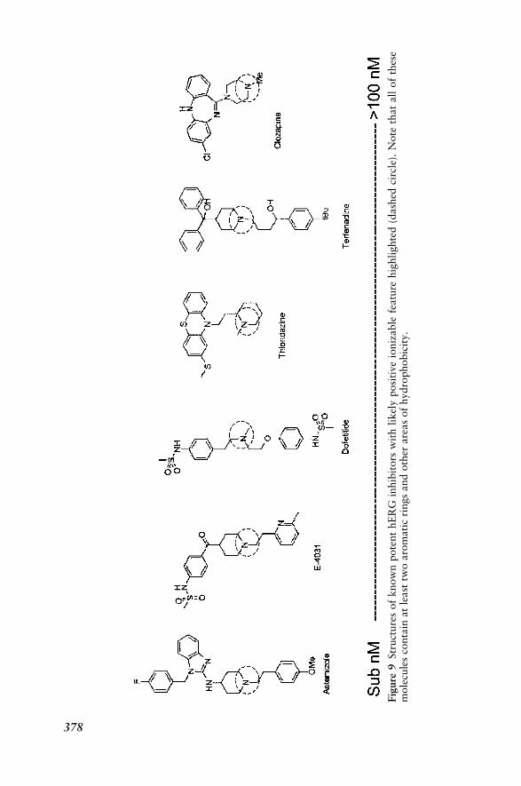
Fig

ure

9Str

uct

ure

sof

know

npote

nt

hE

RG

inhib

itors

wit

hli

kel

yposi

tive

ioniz

able

featu

rehig

hli

ghte

d(d

ash

edci

rcle

).N

ote

that

all

of

thes

em

ole

cule

sco

nta

inat

least

two

aro

mati

cri

ngs

and

oth

erare

as

of

hydro

phobic

ity.

378

obtained with the data from the antipsychotic agents.334 The new pharmaco-phore generated with this literature data set contains four hydrophobes andone positive ionizable feature. This is somewhat different from the antipsychotic-derived pharmacophore in that the aromatic ring feature in the latter model isreplaced with a positive ionizable feature, and, there are more hydrophobes inthe new model. Agreement between the published homology model and thehydrophobic features in both hERG pharmacophores appears to coincidewith the F656 and Y652 residues in the homology model that are involvedin p–p stacking with aromatic residues of the inhibitors.333

The general hERG pharmacophore model based on literature data wasalso assessed using a test set of molecules excluded from the model. Thatdata was generated in our own laboratories. In light of the work presentedin our initial report, it appears that the pharmacophore is able to generate pre-dictions for the 22 molecules (predicted vs. observed r2 ¼ 0:83) and producesa statistically significant rank ordering as indicated by the Spearman’s rhocoefficient of 0.77. Also note that, on the whole, this model predicts someIC50 values to be higher than those observed experimentally but in a few cases,like terfenadine, this is reversed. However, it is important to understand thatthe model is able to correctly rank order the inhibition of parent molecules andmetabolites. Indeed, the model can distinguish between thioridazine and itsmetabolite mesoridazine; clozapine and clozapine N-oxide and N-desmethyl-clozapine; risperidone and 9-hydroxyrisperidone as well as olanzapine andtwo of its metabolites. Furthermore, the general hERG model can distinguishpotent inhibitors of hERG, such as thioridazine (Figure 9), cisapride, and ser-tindole from weaker inhibitors, such as nicotine, desmethyl olanzapine, and 2-hydroxymethyl olanzapine, therefore enabling a ranking of molecules, whichmay be valuable in early drug discovery.334

Protein binding and drug metabolism are also important factors to con-sider when selecting molecules in pharmaceutical design. Protein binding anddrug metabolism are also expected to impact predictions for hERG inhibition.If the drug molecule is tightly bound or extensively metabolized, less of thatparent drug will be available for inhibition of hERG (although in the caseof metabolism the assessment of inhibitory potential of metabolites may beneeded). It has been suggested by Kang et al. that hERG channel inhibitionis not a class effect, at least in the case of fluoroquinolones.335 In Kang’s studyof seven antibiotics for hERG inhibition in oocytes expressing the potassiumchannel, a range of IC50 values from 18 to 1420 mM was produced. This invitro data was also used in conjunction with free plasma concentrations to cal-culate hERG IC50 / plasma concentration ratios. The results indicated thatsome molecules like grepafloxicin, which are known to prolong the QT inter-val in humans, possess low ratios while other molecules like ciprofloxacin havemuch higher ratios and, consequently, do not prolong the QT interval.

Our observations suggest there may be multiple binding interactionswithin the potassium channel ultimately making this difference difficult to

Channels 379

predict and could account for some of our poor predictions. Overcoming thislimitation imposed by multiple-binding interactions may require multiplepharmacophores or platform-specific models (like the antipsychotic derivedmodel described previously) that could detect subtle structural differencesand account for the multiple conformations explored by software like Cata-lyst. To some extent, literature studies have explored platform-specific models.Kang et al.’s study of seven antibiotics with measured hERG IC50 values335

suggested the most potent hERG inhibitors contain C5 substituents. It isunknown how this structure–activity relationship relates to other moleculesfrom different therapeutic areas, thus limiting its applicability. It has been sug-gested by De Ponti et al., that some noncardiac drugs known to be hERG inhi-bitors contain the same structural feature pharmacophore as class-IIIantiarrhythmics (a para-substituted phenyl ring connected to a basic nitrogenby a variable chain) while others do not.336

In an attempt to predict classes of hERG inhibitors using data from Chi-nese hamster ovary (CHO) cells expressing the channel,337 a computationalanalysis found a striking difference in ClogP between potent and nonpotentinhibitors. In agreement with the pharmacophore studies, hydrophobicitywas found to be important for the potent inhibitors. In that study, neural net-work models were generated based on 244 proprietary structures. This neuralnetwork model performed better at identifying the less potent inhibitorsbecause it misclassified some potent inhibitors.337 In another pharmacophorestudy, literature data was used to build a CoMFA model for 31 inhibitors.338

This model contained three aromatic functions as well as a central nitrogenfunction.338 This CoMFA model was in good agreement with the earlierCatalyst pharmacophore as well as the aforementioned homology model forhERG. Some companies are generating inhibition of [3H]-dofetilide bindingdata with hERG for use in a number of projects. For example, researchersat Merck have published two papers containing data for the 5HT2A class ofmolecules339,340 and one relating to 3-aminopyrrolidinone farnesyltransferaseinhibitors341 in which hERG binding was reduced to some extent by structuralmodification. Ultimately, this data may also be used for computational modelbuilding for hERG although the structural diversity of the molecules is limited(Figure 10a–c). Alignment of Catalyst-derived pharmacophores (Figure 10d)generated with this Merck data suggested common areas of positive ionizablefeatures, and hydrophobicity (aromatic rings).

We conclude the discussion on hERG by considering the ability of verylarge naturally occurring molecules like the scorpion toxin BeKm-1 (4092 Da),which acts as a potent and selective inhibitor of hERG (3.3 nM).342 Perhapslarge molecules like this peptide block multiple subunits on hERG, or, theN-terminal domain of the toxin contains a positively charged amino acidthat acts like a stopper and blocks the channel in a single subunit. A recentpaper suggested the most critical residues for binding are located on the alphahelix, which is in contrast to other known scorpion toxins.343 It is interesting


to note that the surface of the protein clearly has an area of positive chargesurrounded by multiple hydrophic areas, which mimics the pharmacophoresdefined for small molecule inhibitors described previously. Clearly, a moleculeof the size of BeKm-1 is outside the scope of existing pharmacophores andother computational models generated to date for hERG, but this has implici-cations for testing protein drugs in vitro as inhibitors of hERG. There is cer-tainly a need for using a diverse array of computational approaches to betterunderstand other ion channels that are important for cardiac function, cellularhomeostasis and communication. To date, relatively few computationalstudies have been done although there are many SAR studies for inhibitorsof calcium and sodium channels in the literature.

Figure 10 Catalyst pharmacophores. generated with Merck published data (H¼hydrophobe; RA¼ ring aromatic;þ ve¼ positive ionizable): (a) for 5HT2A inhibitors

from Fletcher et al.340 data, observed versus predicted r ¼ 0:93. The figure showsinhibitors fitted to the features; (b) for farnesyltransferase inhibitors from Bell et al.341

observed versus predicted r ¼ 0:87; (c) comparison of pharmacophores from (a) and (b)

as well as an additional pharmacophore (i) for 5HT2A inhibitors from Rowley et al.339

observed versus predicted r ¼ 0:87; (d) combination of all three hERG pharmacophoresshowing common regions.

Channels 381

RECEPTORS

As with ion channels a wide diversity of receptors exists that play keyroles in maintaining our physiology. Such receptors can also represent thera-peutic targets. Examples include the a-adrenoreceptor, b-adrenoreceptor,AMPA, NMDA, GABA, serotonin, dopamine, glutamate, histamine, glycine,opiate, NMDA, cannabinoid, and steroid receptors. Nuclear receptors are afamily of ligand-regulated transcription factors that include the glucocorticoidreceptor, the vitamin D receptor, the estrogen receptor, and the so-called‘‘orphan nuclear receptors’’. Interactions with these latter receptors may notbe beneficial as we are now finding out.

Pregnane X-Receptor

Recently, it was discovered that the pregnane X receptor (PXR, alsoknown as SXR or PAR) is a transcriptional regulator of the enzymeCYP3A344–346 and is activated by many of the structurally diverse CYP3Ainducers. This nuclear hormone receptor is just one member of a large familythat acts as a transcription factor in order to regulate induction of numerousgenes. The discovery of PXR provided some degree of understanding for mod-ulation of CYP3A expression in response to endobiotics and xenobiotics.Three years after its discovery the role of PXR was expanded to include theregulation of expression of human MDR1 and CYP2C8/9.347 These discov-eries provided some insight as to how drugs could regulate not only theirown metabolism but potentially their efflux too, as demonstrated for paclit-axel.348 Adding to the complexity of understanding the interindividual varia-bility in the expression and functional response was the identification of 38SNPs. These SNPs were not found in the ligand binding site of human PXR.They could, nonetheless, have important physiological ramifications349 as theysuggest that PXR may have a crucial role in binding an endogenous ligand.350

Recently, PXR was also shown to regulate many other genes involved in thetransport, metabolism, and biosynthesis of bile acids.351

The impact of PXR on drug development is being felt in the pharmaceu-tical industry, which is advocating the use of high throughput assays to elim-inate likely CYP3A inducers early in discovery.352 The extent of use of assaysfor PXR depends on the screening paradigm instituted by each drug companyat the discovery stage. The PXR reporter and functional assays represent a sur-rogate for the in vivo animal assays of induction. These assays have signifi-cantly higher throughput and avoid the complication of extrapolatinganimal in vivo data to human in vivo data. However, the availability of thePXR-null and SXR-transgenic mice represent in vivo models that incorporatehuman PXR with in vivo pharmacokinetics capabilities.353,354 Hence, speciesdifferences in induction may be avoided to some degree. A diversity of mole-cules exist that bind to human PXR in vitro. These ligands include a selection


of bile acids,351,355 statins,356 components of herbal remedies such as hyper-forin found in St. John’s Wort,357,358 human immunodeficiency virus (HIV)protease inhibitors,359 calcium channel modulators,360 steroids,352 plasticizersand monomers,361–363 organochlorine pesticides,364 and a growing list ofdiverse xenobiotics.344–347,352,357,365–368 To some extent, these in vitro find-ings explain in vivo DDIs that in some cases have been known for decadesor in others may have only recently been recognized.

A growing list of PXR ligands now exists and one might think that vir-tually any suitable molecule could be added to this list because the ligand-binding domain is a large, flexible hydrophobic site with a few polar residuesplus three distinct binding sites for SR12813 (as described by X-ray crystallo-graphy354). However, this structural information for the ligand-bindingdomain and structural information about ligands themselves can all be usedto select molecules that avoid binding to this protein. The effect of differentmolecules binding uniquely to PXR was tested by mutating amino acids thatform salt bridges adjacent to the binding cavity when CV-1 cells transfectedwith expression plasmids for PXR were incubated with SR12813 or rifampi-cin. When Asp205 is mutated to Ala, rifampicin becomes a more potent PXRactivator in the reporter gene assay. Similarly, targeted mutants meant to con-fer a human-like response to mouse PXR confirmed the importance of theseresidues in other species. Rather than being responsible for direct bindingwith the ligand it is likely that these residues are altering the shape of the bind-ing site significantly. Flexibility of the binding site probably enables the accep-tance of more structurally diverse ligands that in turn may act as antagonists(like ecteinascidin) and possibly interact with the heterodimer RXR. Therehave been several reports from the same laboratory defining PXR binding interms of EC50.352,355,357 These data for 12 molecules were used to generate apharmacophore with Catalyst. That pharmacophore may define key featuresof ligands that bind to the PXR binding site365 (Figure 11). The pharmaco-phore was also positioned in the human PXR ligand-binding domain. Thispharmacophore was further tested with other PXR ligands for which activation–deactivation data was available. The pharmacophore was also aligned tomatch three binding positions to SR12813365 as implicated from a crystallo-graphy study.354 The PXR pharmacophore provided a good correlationbetween observed and predicted training set data derived from a single labora-tory. It also enabled a qualitative assessment of 28 other molecules, some ofwhich were PXR ligands (CYP3A4 inducers), by predicting EC50 data withinthe range of the training set. This pharmacophore may have defined theminimal set of molecular features needed for binding to this nuclear receptor.It implicates at least four hydrophobic features and at least one hydrogen-bonding feature that should be avoided in future drug candidate molecules.What might be difficult to understand from just a potential ligand structurealone is its binding orientation in the crystal structure. In addition to the threesites identified in SR12813, smaller ligands could have additional binding

Receptors 383

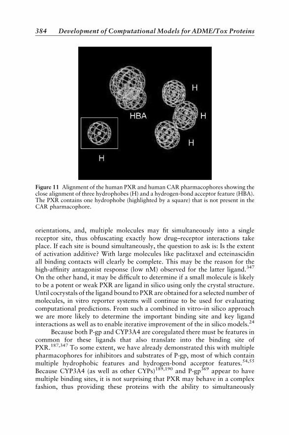
orientations, and, multiple molecules may fit simultaneously into a singlereceptor site, thus obfuscating exactly how drug–receptor interactions takeplace. If each site is bound simultaneously, the question to ask is: Is the extentof activation additive? With large molecules like paclitaxel and ecteinascidinall binding contacts will clearly be complete. This may be the reason for thehigh-affinity antagonist response (low nM) observed for the latter ligand.347

On the other hand, it may be difficult to determine if a small molecule is likelyto be a potent or weak PXR are ligand in silico using only the crystal structure.Until cocrystals of the ligand bound to PXR are obtained for a selected number ofmolecules, in vitro reporter systems will continue to be used for evaluatingcomputational predictions. From such a combined in vitro–in silico approachwe are more likely to determine the important binding site and key ligandinteractions as well as to enable iterative improvement of the in silico models.24

Because both P-gp and CYP3A4 are coregulated there must be features incommon for these ligands that also translate into the binding site ofPXR.187,347 To some extent, we have already demonstrated this with multiplepharmacophores for inhibitors and substrates of P-gp, most of which containmultiple hydrophobic features and hydrogen-bond acceptor features.54,55

Because CYP3A4 (as well as other CYPs)189,190 and P-gp369 appear to havemultiple binding sites, it is not surprising that PXR may behave in a complexfashion, thus providing these proteins with the ability to simultaneously

Figure 11 Alignment of the human PXR and human CAR pharmacophores showing theclose alignment of three hydrophobes (H) and a hydrogen-bond acceptor feature (HBA).The PXR contains one hydrophobe (highlighted by a square) that is not present in theCAR pharmacophore.


handle diverse structures, some of which may result in up-regulation of trans-porters and enzymes to increase the rate of clearance.

The clinical implications from a complete understanding of PXR isbecoming obvious. Our ability to predict potential DDIs that might occur asa result of coadministration of xenobiotic PXR ligands with molecules knownto be metabolized or transported by any of the genes up-regulated at a parti-cular moment in time, becomes possible. Subsequently, the identification ofother genes regulated by PXR has increased. The CYP2B6 enzyme is involvedin the metabolism of many diverse structural classes of drugs,370 and has morerecently been shown to be directly regulated by PXR.371 A further remarkableobservation by Goodwin et al. is that similar levels of induction exist forCYP2B6 and CYP3A4 for four out of five molecules. Both CYP2C8 andCYP2C9 are involved in the regio- and stereoselective epoxidation of arachi-donic acid in the liver and kidney.372 These enzymes have also been shown tobe induced by calcium channel antagonists via PXR.360 The intestinal trans-porter MDR1 induction by rifampicin and other xenobiotics has been shownto be mediated by PXR using the human colon carcinoma cell line LS174T as amodel system.373 Human MRP1 (ABCC1) and MRP2 (ABCC2), which areresponsible for eliminating conjugates of toxic molecules and biliary effluxof endogenous molecules, respectively, have been shown to be induced byredox-active molecules as well as other types of compounds. However, itwas unclear from one study exactly what role PXR might have in the induc-tion374 of these proteins. The enzyme inducible nitric oxide synthase (iNOS) isup-regulated by PXR, thus explaining how steroids affect inflammation.375 Itis possible that genes previously thought to be regulated solely by alternativeligand-activated transcription factors may also be regulated partially via PXR.Endogenous hormones like estradiol are known to be PXR ligands.344–346

They can regulate their own metabolism in hepatic tissues via CYP3A4 andconceivably in extrahepatic tissues via CYP1B1376 or other CYPs simulta-neously. There may also be a developmental role of the orphan nuclear recep-tors (like PXR) in switching on genes at the appropriate time in response toendogenous ligands such as environmental pollutants that are teratogensunder the right conditions.377 This in turn may represent a point at whichthe gene can be interfered with by other molecules, thus preventing abnormalfetal growth. Predicting this activity computationally in the future is clearly ofvalue.

Constitutive Androstane Receptor

A second orphan nuclear receptor, the constitutive androstane receptor(CAR), has � 40% identity with PXR in the ligand-binding domain. MurineCAR was found to be inhibited (EC50 < 500 nM) by the androstane metabo-lites androstanol and androstenol,378 which are most likely the endogenousrepressors.379 Following exposure to phenobarbital, CAR accumulates in the

Receptors 385

nucleus, heterodimerizes with RXR, binds to the two phenobarbital responsiveelements and ultimately activates transcription of the CYP2B genes.380 HumanCAR was found to be activated by the pesticide TCPOBOP, phenobarbital,chlorpromazine, O,P0-DDT, methoxychlor, and PCB. This activation corre-sponded well with the induction of the CYP2B6 gene.381 Other ligands forhuman CAR including clotrimazole and the progesterone metabolite 5a-preg-nane-3,20-dione have been described. Androstanol is a less potent activatorfor human CAR compared to mouse CAR.382 Murine CAR is also activatedby metyrapone and clotrimazole.383 CAR appears to activate other genesbesides CYP2B6 including CYP3A4381 in a manner similar to how PXR canactivate CYP2B6 as well as CYP3A4.371 The induction of drug metabolizingenzymes via CAR has also been demonstrated in vivo in mice, while CARknockout mice have an altered sensitivity to inducers.384

So far, it appears that the human PXR ligand-binding domain accomo-dates very large molecules that have the highest reported affinities (e.g., ectei-nascidin IC50¼ 3 nM347) while small planar molecules like steroids and bileacids bind with a much lower affinity.355,382 In comparison large moleculeslike 1,4-bis[2-(3,5-dichloropyridyloxy)]benzene (TCPOBOP) do not bindeffectively to human CAR but do bind to murine CAR,382 while more compactmolecules like clotrimazole bind well as a deactivator to human CAR but notto mouse CAR.382 Interestingly, both the human PXR and CAR share only70% amino acid identity with their homologues in other species382,385,386

and alignments to the human crystal structure for the PXR ligand-bindingdomain clearly show there are some marked differences across the receptorsand between species. This suggests that although there might be some per-ceived overlap in the binding affinity of both human CAR and PXR for thesame ligands, there ultimately may be some significant cross-receptor differ-ences in binding affinity. Therefore molecules like the bile acid metabolitesthat activate PXR with low affinity could have a higher affinity towardCAR or other nuclear hormone receptors. The ability for murine CAR tobind agonists and antagonists of differing size has not gone unnoticed387 whilethe same facility for human CAR has not really been explored. The overlapbetween the receptors has an added functional consequence in sensing the levelof ligand-binding and possibly responding to a different extent depending onthe amount of ligand bound. Hence, the body retains high-affinity nuclear hor-mone receptors and low-affinity nuclear hormone receptors for structurallysimilar molecules to more efficiently regulate metabolism and efflux or toretain a steady state. The complexity of this system comes about when extra-polating to the in vivo state from the well-defined in vitro models. At this point intime the key question is: Does what we observe in vitro really translate to in vivo?

As more data is generated about CARs involvment in the inductionof CYP2B,388 CYP3A,381 and possibly other genes, computational modelswill likely be generated for the ligands and inhibitors. At present a simplealignment of five molecules suggested to be mouse CAR activators


(chlorpromazine, clotrimazole, metyrapone, TCPOBOP, and phenobarbi-tal383) yield a pharmacophore with two hydrophobic features and one hydro-gen-bond acceptor.226 This planar model appears to indicate that CAR is a lesspromiscuous receptor than PXR because it accommodates less flexibility in theligands involved in activation. This hypothesis is based on the finding thatCAR has high affinity for the rigid repressors and androstane metabolitesthat appear to also fit well within the confines of this model.378 To some extentthis in silico finding may help answer the question as to whether or not and-rostanes bind directly to CAR.367 On the basis of this small pharmacophorethe answer appears to be yes they do. When three molecules with knownEC50 values for human CAR (clotrimazole, androstanol, and 5a-pregnane-3,20-dione382) were used to build a pharmacophore, a model consisting ofthree hydrophobes and one hydrogen-bond acceptor was generated.226 Thismodel parallels a previously described human CYP2B6 substrate pharmaco-phore,100 which consists of the same features in a similar arrangement.When the human PXR pharmacophore (generated with Catalyst version 4.6and fast conformer generation) and human CAR pharmacophores are mergedtogether there exists some overlap of the hydrogen binding and hydrophobicfeatures. But, there appears to be one less hydrophobe in the CAR model (Fig-ure 11)226 indicating a smaller binding site. A smaller binding site is consistentwith a recent analysis of the binding cavity surface volumes of CAR (1170 A3)and PXR (1220 A3) using GRASP.389 When the potent ligand 5a-pregnane-3,20 dione is fitted to the human CAR pharmacophore along with the bileacids that are identified as low-affinity PXR ligands355 (e.g., lithocholic acidand ketolithocholic acid), it can be seen that there is some overlap betweenthem.226 This may imply that potent steroid ligands and related bile acidscould be higher affinity ligands (activators or repressors) for CAR than forPXR. This speculation needs experimental verification, however. It is appro-priate to relate this observation back to the major genes that each orphannuclear receptor regulates, namely, CYP2B6 and CYP3A4. A molecule couldpotentially regulate both enzymes via different receptors, to differing extentssimultaneously. The similarity of the pharmacophore for CAR with that ofhuman CYP2B6100 once again suggests that ligands for an enzyme (or trans-porter) have features in common with the ligands for the receptor responsiblefor regulating it as described for PXR.365,390 By using the human PXR crystalstructure as a template to align human CAR, it can be shown how a single ami-no acid, Phe161, can block SR12813 from binding, thus drastically reducingthe volume of the CAR binding site compared with that of PXR in whichMet243 is in the same position. The steric interactions that are describedfor SR12813 would ultimately suggest that binding to CAR is unfavorable,as actually found in vitro.382 Four ligands have been docked in the homologymodel for CAR using GOLD. As with PXR it is found that there could be mul-tiple binding modes.389 In all cases, the ligands were suggested to interact withPhe161 as well as with other residues.

Receptors 387

An impediment to our understanding of the roles of CAR and PXRcomes in the form of submicromolar concentrations of glucocorticoids likedexamethasone, which increase PXR, CAR, and RXR expression in humancultured hepatocytes and ultimately result in increased CYP expression andresponse.391–393 Pascussi et al. suggest that glucocorticoids may control hepa-tic expression of PXR and CAR and are responsible for basal CYP3A4 expres-sion in the absence of inducers. Upon challenge with an inducer, thesereceptors are also activated and increase CYP3A4 expression.391–393 The evi-dence Pascussi et al.392 tender is that dexamethasone has been shown to beneither a CAR nor a PXR ligand at submicromolar levels. Those authorsalso propose instead that it acts via the glucocorticoid receptor to up-regulatePXR and CAR, which then acts on CYP3A4. This research group has alsoshown that a strong correlation exists between the expression levels of PXR,CAR, and CYP3A4 in human liver microsomes. This contrasts with the experi-mental data derived from CAR and PXR knockout animals that do not showany loss of CYP3A4,353,355,384,394,395 indicative of dexamethasone playing norole in basal regulation for either of these receptors.

By limiting our discussion to just two nuclear receptors, we have avoidedthe complicated issue of how other nuclear receptors may be involved in theregulation of many key enzymes and transporters. Coming to terms with thecomplexity of the regulation of the many key proteins important for ADME/Tox processes can be accomplished with the help of molecular modeling.226

FUTURE DEVELOPMENTS

The increased level of interest in computational models for ADME/Toxis influenced by the need that multinational pharmaceutical companies nowhave to lower costs396 and to increase the width of their discovery pipelines.The risks and expenses associated with developing drugs has increased to thepoint where companies have pulled forward to early development stagesscreens for ADME/Tox properties. These companies have started to utilizecomputational filters early on in their bid to lower costs and to improve theefficiency of developing molecules.397

Given the growing number of computational models for ADME/Toxproperties as well as new data sets that are being published we may soon reacha point where other algorithmic technologies could be considered to createknowledge from those data sets. In addition to the various types of 3D-QSAR models already described in this chapter, there are those that havebeen developed using a genetic algorithm to simulate metabolic transforma-tions.398 Also, predictive models have been generated by taking into accountthe electronic properties of molecules like those with the tendency for oxi-dation (P450 mediated hydrogen-atom abstraction). These predictive models,based on this alternative modeling approach, have been used for both rat and


human enzymes.51,399,400 In addition a number of rule-based tools have beendeveloped to predict metabolism using the same concepts implemented fortoxicity prediction.53 One approach has used a metabolic fingerprint (META-PRINT) that uses a rule-based system (MetabolExpert) that outputs informa-tion on 179 metabolic transformations that can then be used for similaritysearching and cassette dosing experiments.401 The study initially describingthis used a validation set of five compounds and it remains to be seen whetherthis type of rule based approach will become more widely used.

High throughput docking has recently been used with CYPcam and ahomology model of CYP3A4. Using the GOLD, DOCK, PMF, and FlexXscoring functions an attempt was made to predict known substrates and inhi-bitors.402 Of the 345 compounds evaluated, 334 had GOLD scores less than�100. However, this study was not able to differentiate between substratesand inhibitors of CYP3A4.402 There have also been attempts to use an affinityfingerprint to train a QSAR.327,403–405 The generation of protein affinity fin-gerprint models has the potential for use with ADME/Tox-related proteins.405

The validity and utility of this method remains to be seen, however. The devel-opment406–408 and evaluation409–411 of various knowledge-based potentialsfor scoring ligand-binding within proteins combined with de novo design toolsand ADME/Tox filters represents the next level of evolution for drug discov-ery. The simultaneous design of molecules within the target binding site alongwith optimally predicted ADME/Tox properties would have a considerableimpact in molecular design.412 With considerable interest in using numerousin vitro data sets and computational technologies for modeling and ultimatelyunderstanding G-protein-coupled receptors that are therapeutic targets,413 wemay better comprehend the structural features and dynamics of the manytransporters and receptors that to date have eluded all efforts at crystalliza-tion. Some techniques have been developed recently to predict the tertiarystructure of proteins from their amino acid sequence. Complementing thisare new methods for predicting the binding site and binding energy of ligandsto GPCRs.124 Some success along these lines has been shown by Shachamet al.414 who could reproduce the crystal structure of the only known exampleof a 7-transmembrane protein, rhodopsin. Such technology could be appliedelsewhere. Complexity in ligand–protein interactions should not be underesti-mated and there is a shift toward thinking of some proteins as existing in apopulation of many conformations.415 Clearly, the complexity of interactionsand kinetics noted for CYP3A4, P-gp, and PXR and perhaps other ADME/Toxrelated proteins will require identifying these conformations. This may lead tocomputational predictions and algorithms that can be applied elsewhere.

New visualization technologies416 and algorithms for descriptor selec-tion for ADME/Tox models are also important in the development of the field.The recent description of ‘‘particle swarms’’ that explore the search spacethrough a population of individuals that adapt and return to previously suc-cessful regions has been used for feature selection.73 Although not yet fully

Future Developments 389

described in the literature, particle swarms may be combined with other algo-rithms for use in selecting appropriate (and potentially novel) ADME/Toxdescriptors before model building. The relatively recent development of sup-port vector machines (SVM) for classification problems may add another com-putational tool to the list available for ADME/Tox modeling. The theorybehind this approach has been well described417 and SVM has been appliedto microarray gene expression data.418,419 The use of SVM for pattern classi-fication in QSAR has recently been described and compared with artificialneural networks for antistamine and antibacterial data sets.420 SVM hasalso been used with drug discovery data sets in which the molecules weredescribed with > 100,000 descriptors.421 This approach may be useful forderiving ADME/Tox models from very large data sets although a careful eva-luation of these approaches with well-known data sets may be necessary toshow that they are better than existing and more commonly used technologies.This type of analysis could be facilitated by the creation of a publically avail-able website for ADME/Tox datasets, molecular descriptors, and computa-tional models that could be used by researchers in both academia andindustry. Although efforts by the National Cancer Institute and the Environ-mental Protection Agency are being made to make available toxicity data sets,there has been no effort as yet to do this for ADME models. We could envisiondata sets for nonproprietary molecules with solubility, BBB, metabolism, andrelated data in a single location. It may be in the interest of the companies mar-keting computational software to sponsor these webpages as well as theirworking toward a standard for display and utilization of models in muchthe same way as various Markup languages have developed. As it standsnow it would take a motivated and knowledgeable individual an enormousamount of time and many tens of thousands of dollars to start buildingADME/Tox models just from literature data. Moreover, unless collaboratorsuse the same software it is almost impossible to share models. If this barrierwas removed, the threshold for entry into the drug discovery business couldbe dramatically lowered. At the same time we could be making all the piecesof virtual drug discovery from library generation, virtual screening, scoring,and selection algorithms available to the public (assuming that such toolswill be used for the common good of society). At the same time that computa-tional biologists are working toward standards for development of models,should not those of us in the field of computational chemistry and computa-tional ADME/Tox be doing the same? Doing this may not be as unrealistic asit seems.

The future of computational ADME/Tox requires integrated approachesthat automatically update computational models as data is being generatedfrom the various in vitro assays. This needs to be done in such a way thatthe transition from data generation to data storage to computational modelingis seamless as depicted in Figure 1. This seamless interconnection is actuallyclose to reality due to the database software now available. ADME/Tox model


building consists of a pathway in which several steps have equal importance.For successful ADME/Tox modeling, we list our ‘‘ten commandments’’ in Fig-ure 12. This process and our commandments would be applicable to manyADME/Tox properties as well as for bioactivity models that at present bothundergo multiple sequential screening cycles.422 At some point, a limit willbe reached in terms of the model’s predictive ability. This depends on thestructural diversity of the data set, its representation of chemistry space andthat of the molecules it is predicting. There perhaps needs to be some investi-gation of how many molecules and what level of diversity a model should pos-sess for maximum utility. Molecular descriptor-based models are developingalongside pharmacophore-based models for predicting DDI.24,97–99 The lattermodels will have a greater viability within a structural series while the formermodels are more amenable to rapid screening of diverse chemotypes althoughthere have been some successes in generating models from diverse structuresand building pharmacophores with quite general predictivity. Even when thereis some complexity in the kinetics or behavior of the enzyme, receptor, chan-nel, or transporter, models built with data from different substrate probes andfrom in vitro studies may be used in combination to first score new moleculesand then to generate some degree of consensus and classification.

Two areas are in urgent need of study. First, understanding how the pre-dictions from multiple models may be combined or related in a logical fashionis important. There may be no single optimal way to combine the data for mul-tiple predictions but as we have previously described there are tools availableto do this.25 How we weight the models may depend on the therapeuticarea targeted and our confidence in the biological data and the models selected

Figure 12 The 10 commandments of ADME/Tox model building.

Future Developments 391

(Figure 2). Second, we must find a way to evaluate cutoff criteria for modelacceptability. This evaluation will depend to some extent on the biological,ADME/Tox antitarget under study.

The next generation of scientists must be able to communicate not onlyin the language of experimental biology but also that of computational biologyand medicinal chemistry. The ability to do this depends very much on thesupport of academic institutions that need to introduce all of the availabletechnologies that are now available as well as those that will be developedin the near future. The key skills we envision as being especially importantto computational studies in ADME/Tox are:

1. Biological knowledge as applied to computational chemistry.2. Some basic understanding of computational chemistry and biology software

and operating systems.3. Flexibility in switching between different modeling approaches (such as

3D-QSAR and statistical methods).4. Awareness of the experimental implications of the ADME/Tox related

protein being studied.5. Understanding of ADME/Tox in vitro and in vivo models.6. An ability to communicate with scientists in both ADME, drug safety,

computational chemistry, discovery chemistry, discovery biology, biosta-tistics, and information technology groups.

7. An understanding that the quality of data being used is key to optimalmodel building.

The very existence of the pharmaceutical industry will become even morereliant on the computational approaches that have been developed over thepast decade in addition to those that are being developed and appliednow. We will rely on computational models to help understand how key pro-teins that determine ADME/Tox properties work and we will use that knowl-edge for the purposes of developing drugs with better biopharmaceuticalproperties.

ACKNOWLEDGMENTS

We are especially thankful for the support and collaboration of the following people andfunding agencies: Dr. Maggie Hupcey, Dr. Stephen H. Wright and Dr. Dallas Bednarczyk(University of Arizona), Dr. Brian Ethell and Dr. Brian Burchell (University of Dundee),Dr. J. Andrew Williams and Dr. Marcel de Groot (Pfizer), Dr. David Stresser (BD Gentest),Dr. Richard Kim (Vanderbilt University), Dr. Erin G. Schuetz (St Jude Children’s ResearchHospital), Dr. Leonid Mirny (MIT), Mr. Richard Snyder (Butler University), Dr. Bruno Boulanger,Mr. James H. Wikel, Dr. Jibo Wang, Dr. Anne Dantzig, Dr. Jon Erickson, Dr. Steven A. Wrighton(all at Eli Lilly and Company), Dr. Bruce D. Hammock (UC, Davis) and Dr. Michael W. Duffel(University of Iowa). PWS also acknowledges research support from NIH DK56631 andDK061425, Mr. Cheng Chang and Mr. Yongheng Zhang and Dr. Jash Unadkat (University ofWashington).


ABBREVIATIONS

QSAR, Quantitative structure–activity relationship; sEH, cytosolic epoxide hydrolase;CYP, cytochrome P450; CAR, constitutive androstane receptor; PXR, pregnane X receptor;hERG, human ether-a-gogo related gene; P-gp, P-glycoprotein; MAO, monoamine oxidase;FMO, Flavin-containing monooxygenase.

REFERENCES

1. S. Ekins, C. L. Waller, P. W. Swaan, G. Cruciani, S. A. Wrighton, and J. H. Wikel,J. Pharmacol. Toxicol. Methods, 44, 251 (2000). Progress in Predicting Human ADMEParameters in Silico.

2. S. Ekins and J. P. Rose, J. Mol. Graph., 20, 305 (2002), in Silico ADME/TOX: The State of theArt at the 220th ACS Meeting.

3. M. D. Wessel and S. Mente, Ann. Rep. Med. Chem., 36, 257 (2001). ADME by Computer.

4. D. Butina, M. D. Segall, and K. Frankcombe, Drug Disc. Today, 7, S83 (2002). PredictingADME Properties in Silico: Methods and Models.

5. S. Ekins, J. Maenpaa, and S. A. Wrighton Handbook of Drug Metabolism; Marcel Dekker,New York, 1999; pp. 363–399. In Vitro Metabolism: Subcellular Fractions.

6. D. R. Nelson, L. Koymans, T. Kamataki, J. J. Stegeman, R. Feyereisen, D. J. Waxman, M. R.Waterman, O. Gotoh, M. J. Coon, R. W. Estabrook, I. C. Gunsalus, and D. W. Nebert,Pharmacogenetics, 6, 1 (1996). P450 Superfamily: Update on New Sequences, GeneMapping, Accession Numbers and Nomenclature.

7. E. Y. Zhang, M. A. Phelps, C. Cheng, S. Ekins, and P. W. Swaan, Adv. Drug Del. Rev., 54, 329(2002). Modeling of Active Transport Systems.

8. M. A. Hediger, M. J. Coady, T. S. Ikeda, and E. M. Wright, Nature (London) 330, 379 (1987).Expression Cloning and cDNA Sequencing of the Naþ /Glucose Cotransporter.

9. M. A. Hediger, T. Ikeda, M. Coady, C. B. Gundersen, and E. M. Wright, Proc. Natl. Acad. Sci.U.S.A., 84, 2634 (1987). Expression of Size-Selected mRNA Encoding the Intestinal Na/Glucose Cotransporter in Xenopus laevis Oocytes.

10. M. H. Saier, Jr., Int. Rev. Cytol., 190, 61 (1999). Eukaryotic Transmembrane SoluteTransport Systems.

11. M. Dean, A. Rzhetsky, and R. Allikmets, Genome Res, 11, 1156 (2001). The Human ATP-Binding Cassette (ABC) Transporter Superfamily.

12. P. W. Swaan, S. Oie, and F. C. Szoka, Jr., Adv. Drug. Del. Rev., 20, 1 (1996). Carrier-Mediated Oral Drug Delivery—Preface.

13. P. W. Swaan, S. Oie, and F. C. Szoka, Jr., Adv. Drug Del. Rev., 20, 59, (1996). Use of theIntestinal and Hepatic Bile Acid Transporters for Drug Delivery.

14. P. W. Swaan, K. M. Hillgren, F. C. Szoka, Jr., and S. Oie, Bioconjug. Chem., 8, 520 (1997).Enhanced Transepithelial Transport of Peptides by Conjugation to Cholic Acid.

15. C. J. Blankley, Pharm. Pharmacol. Commun., 4, 139 (1998). Measuring Molecular Diversity:Evaluation of Alternative Subsets Selected from Reagent Building Block Libraries forCombinatorial Chemistry.

16. Y. C. Martin, M. G. Bures, and R. D. Brown, Pharm. Pharmacol. Commun., 4, 147 (1998).Validated Descriptors for Diversity Measurements and Optimization.

17. J. Sadowski, Pharm. Pharmacol. Commun., 4, 153 (1998). Methods for Selecting Compoundsfrom Molecular Databases.

18. H. Kubinyi, Pharmazie, 50, 647 (1995). Strategies and Recent Technologies in DrugDiscovery.

References 393

19. H. Kubinyi, Drug Disc. Develop., 1, 4 (1998). Structure-Based Design of Enzyme Inhibitorsand Receptor Ligands.

20. H. Kubinyi, Drug Disc. Develop., 1, 16 (1998). Combinatorial and ComputationalApproaches in Structure-Based Drug Design.

21. T. Fujita, Quant. Struct. Act. Relat., 16, 107 (1997). Recent Success Stories Leadingto Commercializable Bioactive Compounds with the Aid of Traditional QSARProcedures.

22. S. Ekins, B. J. Ring, G. Bravi, J. H. Wikel, and S. A. Wrighton, Pharmacophore Perception,Development, and use in Drug Design; IUL, San Diego, 2000, pp. 269–299. PredictingDrug–Drug Interactions in Silico Using Pharmacophores: A Paradigm for the NextMillennium.

23. S. Ekins and S. A. Wrighton, J. Pharm. Tox. Methods, 44, 1 (2001). Application of in SilicoApproaches to Predicting Drug–Drug Interactions: A Commentary.

24. S. Ekins, M. de Groot, and J. P. Jones, Drug Metab. Dispos., 29, 936 (2001). Pharmacophoreand Three Dimensional Quantitative Structure Activity Relationship Methods for ModelingCytochrome P450 Active Sites.

25. S. Ekins, B. Boulanger, P. W. Swaan, and M. A. Z. Hupcey, J. Comput. Aided. Mol. Des., 16,381 (2002). Towards a New Age of Virtual ADME/TOX and Multidimensional DrugDiscovery.

26. M. D. Barratt, Environ. Health Perspectives, 106, 459 (1998). Integration of QSAR and InVitro Toxicology.

27. M. D. Barratt and R. A. Rodford, Curr. Opin. Chem. Biol., 5, 383 (2001). The ComputationalPrediction of Toxicity.

28. M. T. Cronin, Pharm. Pharmacol. Commun., 4, 157 (1998). Computer-Aided Prediction ofDrug Toxicity in High Throughput Screening.

29. D. E. Johnson, P. E. Blower, Jr., G. J. Myatt, and G. H. I. Wolfgang, Curr. Opin. Drug Disc.Dev., 4 (2001). Chem-Tox Informatics: Data Mining Using a Medicinal Chemistry BlockApproach.

30. D. E. Johnson and G. H. I. Wolfgang, DDT, 5, 445 (2000). Predicting Human Safety:Screening and Computational Approaches.

31. C. A. Lipinski, Curr. Drug Disc., April, 17 (2001). Avoiding Investment in Doomed Drugs. IsPoor Solubility an Industry Wide Problem?

32. C. A. Lipinski, F. Lombardo, B. W. Dominy, and P. J. Feeney, Adv. Drug Del. Rev., 23, 3(1997). Experimental and Computational Approaches to Estimate Solubility and Perme-ability in Drug Discovery and Development Settings.

33. F. Lombardo, J. F. Blake, and W. J. Curatolo, J. Med. Chem., 39, 4750 (1996). Computationof Brain–Blood Partitioning of Organic Solutes via Free Energy Calculations.

34. U. Norinder and M. Haeberlein, Adv. Drug Del. Rev., 54, 291 (2002). ComputationalApproaches to the Prediction of the Blood–Brain Distribution.

35. U. Norinder, P. Sjoberg, and T. Osterberg, J. Pharm. Sci., 87, 952 (1998). TheoreticalCalculation and Prediction of Brain–Blood Partitioning of Organic Solutes Using MolSurfParameterization and PLS Statistics.

36. A. George, Curr. Opinion Drug Disc. Dev., 2, 286 (1999). The Design and MolecularModeling of CNS Drugs.

37. T. Sanghvi, N. Ni, and S. H. Yalkowsky, Pharm. Res., 18, 1794 (2001). A Simple ModifiedAbsorption Potential.

38. F. Lombardo, M. Y. Shalaeva, K. A. Tupper, and F. Gao, J. Med. Chem., 44, 2490 (2001).ElogDoct: A Tool for Lipophilicity Determination in Drug Discovery. 2. Basic and NeutralCompounds.

39. F. Lombardo, M. Y. Shalaeva, K. A. Tupper, F. Gao, and M. H. Abraham, J. Med. Chem., 43,2922 (2000). ElogPoct A Tool for Lipophilicity Determination in Drug Discovery.


40. R. Saiakhov, L. R. Stefan, and G. Klopman, Persp. Drug Disc. Design, 19, 133 (2000).Multiple Computer-Automated Structure Evaluation Model of the Plasma Protein BindingAffinity of Diverse Drugs.

41. G. Colmenarejo, A. Alvarez-Pedraglio, and J.-L. Lavandera, J. Med. Chem., 44, 4370(2001). Cheminformatic Models to Predict Binding Affinities to Human SerumAlbumin.

42. F. Lombardo, R. S. Obach, M. Y. Shalaeva, and F. Gao, J. Med. Chem., 45, 2867 (2002).Prediction of Volume of Distribution Values in Humans for Neutral and Basic Drugs UsingPhysicochemical Measurements and Plasma Protein Binding.

43. C. Quinones, J. Caceres., M. Stud, and A. Martinez, Quant. Struct. Act Relationship, 19, 448(2000). Prediction of Drug Half-Life Values of Antihistamines Based on the CODES/NeuralNetwork Model.

44. S. Ekins and R. S. Obach, J. Pharmacol. Exp. Thera., 295, 463 (2000). Three Dimensional-Quantitative Structure Activity Relationship. Computational Approaches to Prediction ofHuman In Vitro Intrinsic Clearance.

45. C. L. Waller, M. V. Evans, and J. D. McKinney, Drug Metabolism Disposition, 24, 203(1996). Modeling the Cytochrome P450-Mediated Metabolism of Chlorinated VolatileOrganic Compounds.

46. W. J. Egan, K. M. J. Merz, and J. J. Baldwin, J. Med. Chem., 43, 3867 (2000). Prediction ofDrug Absorption Using Multivariate Statistics.

47. P. Stenberg, K. Luthman, and P. Artursson, J. Controlled Release, 65, 231 (2000). VirtualScreening of Intestinal Permeability.

48. P. Stenberg, U. Norinder, K. Luthman, and P. Artursson, J. Med. Chem., 44, 1927 (2001).Experimental and Computational Screening Models for the Prediction of Intestinal DrugAbsorption.

49. S. Ekins, G. L. Durst, R. E. Stratford, D. A. Thorner, R. Lewis, R. J. Loncharich, and J. H.Wikel, J. Chem. Inf. Comput. Sci., 41, 1578 (2001). Three Dimensional QuantitativeStructure Permeability Relationship Analysis for a Series of Inhibitors of RhinovirusReplication.

50. M. D. Wessel, P. C. Jurs, J. W. Tolan, and S. M. Muskal, J. Chem. Inf. Comput. Sci., 38, 726(1998). Prediction of Human Intestinal Absorption of Drug Compounds from MolecularStructure.

51. J. P. Jones and K. R. Korzekwa, Predicting the Rates and Regioselectivity of ReactionsMediated by the P450 Superfamily., Academic Press, Inc., New York, 1996, pp. 326–335.

52. J. P. Jones, M. Shou, and K. R. Korzekwa, Biochemistry, 34, 6956 (1995). StereospecificActivation of the Procarcinogen Benzo[a]pyrene: A Probe for the Active Sites of theCytochrome P450 Superfamily.

53. J. Langowski and A. Long, Adv. Drug Del. Rev., 54, 407 (2002). Computer Systems for thePrediction of Xenobiotic Metabolism.

54. S. Ekins, R. B. Kim, B. F. Leake, A. H. Dantzig, E. Schuetz, L.-B. Lan, K. Yasuda, R. L.Shepard, M. A. Winter, J. D. Schuetz, J. H. Wikel, and S. A. Wrighton, Mol. Pharmacol., 61,974 (2002). Application of Three Dimensional Quantitative Structure–Activity Relation-ships of P-Glycoprotein Inhibitors and Substrates.

55. S. Ekins, R. B. Kim, B. F. Leake, A. H. Dantzig, E. Schuetz, L.-B. Lan, K. Yasuda, R. L.Shepard, M. A. Winter, J. D. Schuetz, J. H. Wikel, and S. A. Wrighton, Mol. Pharmacol., 61,964 (2002). Three Dimensional Quantitative Structure–Activity Relationships of Inhibitorsof P-Glycoprotein.

56. T. Osterberg and U. Norinder, Eur. J. Pharm. Sci., 10, 295 (2000). Theoretical Calculationand Prediction of P-Glycoprotein-Interacting Drugs Using MolSurf Parameterization andPLS Statistics.

57. T. R. Stouch and O. Gudmundsson, Adv. Drug Del. Rev., 54, 315 (2002). Progress inUnderstanding the Structure–Activity Relationships of P-Glycoprotein.

References 395

58. J. E. Penzotti, M. L. Lamb, E. Evenson, and P. D. J. Grootenhuis, J. Med. Chem., 45, 1737(2002). A Computational Ensemble Pharmacophore Model for Identifying Substrates ofP-Glycoprotein.

59. N. Greene, Adv. Drug Del. Rev., 54, 417 (2002). Computer Systems for the Prediction ofToxicity: An Update.

60. O. Llorens, J. J. Perez, and H. O. Villar, J. Med. Chem., 44, 2793 (2001). Toward the Designof Chemical Libraries for the Mass Screening Biased Against Mutagenic Compounds.

61. S. S. Young, V. K. Gombar, M. R. Emptage, N. F. Cariello, and C. Lambert, Chemo. Intell.Lab. Sys., 60, 5 (2002). Mixture Deconvolution and Analysis of Ames Mutagenicity Data.

62. A. E. M. F. Soffers, M. G. Boersma, W. H. J. Vaes, J. Vervoort, B. Tyrakowska, J. L. M.Hermens, and I. M. C. M. Rietjens, Toxicol. in vitro, 15, 539 (2001). Computer-Modeling-Based QSARs for Analyzing Experimental Data on Biotransformation and Toxicity.

63. C. A. Lipinski, J. Pharm. Toxicol. Methods, 44, 235 (2000). Drug-Like Properties and theCauses of Poor Solubility and Poor Permeability.

64. D. F. Veber, S. R. Johnson, H.-Y. Cheng, B. R. Smith, K. W. Ward, and K. D. Kopple, J. Med.Chem., 45, 2615 (2002). Molecular Properties that Influence the Oral Bioavailability ofDrug Candidates.

65. V. J. Gillet, P. Willett, and J. Bradshaw, J. Chem. Inf. Comput. Sci., 38, 165 (1998).Identification of Biological Activity Profiles Using Substructural Analysis and GeneticAlgorithms.

66. J. Sadowski and H. Kubinyi, J. Med. Chem., 41, 3325 (1998). A Scoring Scheme forDiscriminating Between Drugs and Nondrugs.

67. T. I. Oprea, A. M. Davis, S. J. Teague, and P. D. Leeson, J. Chem. Inf. Comput. Sci., 41, 1308(2001). Is there a Difference between Leads and Drugs? A Historical Perspective.

68. G. W. Bemis and M. A. Murcko, J. Med. Chem., 39, 2887 (1996). The Properties of KnownDrugs. 1. Molecular Frameworks.

69. G. W. Bemis and M. A. Murcko, J. Med. Chem., 42, 5095 (1999). Properties of Known Drugs.2. Side Chains.

70. O. Roche, P. Schneider, J. Zuegge, W. Guba, M. Kansy, A. Alanine, K. Bleicher, F. Danel,E.-M. Gutknect, M. Rogers-Evans, W. Neidhart, H. Stalder, M. Dillon, E. Sjogren, N.Fotouhi, P. Gillespie, R. Goodnow, W. Harris, P. Jones, M. Taniguchi, S. Tsujii, W. vonder Saal, G. Zimmermann, and G. Schneider, J. Med. Chem., 45, 137 (2002). Developmentof A Virtual Screening Method for Identification of ‘‘Frequent Hitters’’ in CompoundLibraries.

71. S. L. McGovern, E. Caselli, N. Grigorieff, and B. K. Shoichet, J. Med. Chem., 45, 1712 (2002).A Common Mechanism Underlying Promiscuous Inhibitors from Virtual and High-Throughput Screening.

72. M. F. M. Engels and P. Venkatarangan, Curr. Opin. Drug Disc. Dev., 4, 275 (2001). SmartScreening: Approaches to Efficient HTS.

73. D. K. Agrafiotis and W. Cedeno, J. Med. Chem., 45, 1098 (2002). Feature Selection forStructure-Activity Correlation Using Binary Particle Swarms.

74. V. J. Gillet, W. Khatib, P. Willett, P. J. Fleming, and D. V. S. Green, J. Chem. Inf. Comput. Sci.,42, 375 (2002). Combinatorial Library Design Using a Multiobjective Genetic Algorithm.

75. W. P. Walters, M. T. Stahl, and M. A. Murcko, Drug Disc. Today, 3, 160 (1998). VirtualScreening-an Overview.

76. A. R. Leach and M. M. Hann, Drug Disc. Today, 5, 326 (2000). The in Silico World of VirtualLibraries.

77. H. Kubinyi, Drug Discovery Today, 2, 457 (1997). QSAR and 3D QSAR in Drug Design.Part1: Methodology.

78. H. Kubinyi, Drug Discovery Today, 2, 538–546 (1997). QSAR and 3D QSAR in Drug Design.Part 2: Applications and Problems.


79. T. I. Oprea and C. L. Waller in Reviews in Computational Chemistry; K. B. Lipkowitz, and D.B. Boyd, Eds.; Wiley-VCH, Wiley, New York, 1997, pp. 127–182. Theoretical and PracticalAspects of Three-Dimensional Quantitative Structure—Activity Relationships.

80. C. Hansch, E. J. Lien, and F. Helmer, Arch. BioChem. Biophys., 128, 319 (1968). Structure–Activity Correlations in the Metabolism of Drugs.

81. C. Hansch, Drug Metab. Rev., 1, 1 (1972). Quantitative Relationships between LipophilicCharacter and Drug Metabolism.

82. C. Hansch, Drug Metab. Rev., 15, 1279 (1984). The QSAR Paradigm in the Design of LessToxic Molecules.

83. C. Hansch, D. Hoekman, and H. Gao, Chem. Rev., 96, 1045 (1996). Comparative QSAR:Toward a Deeper Understanding of Chemicobiological Interactions.

84. C. Hansch and L. Zhang, Drug Metab. Rev., 25, 1 (1993). Quantitative Structure–ActivityRelationships of Cytochrome P-450.

85. D. F. V. Lewis, Toxicology, 144, 197 (2000). Structural Characteristics of Human P450sInvolved in Drug Metabolism: QSARs and Lipophilicity Profiles.

86. D. F. V. Lewis, Biochem. Pharmacol., 60, 293 (2000). On the Recognition of MammalianMicrosomal Cytochrome P450 Substrates and Their Characteristics.

87. D. F. V. Lewis, P. J. Eddershaw, M. Dickins, M. H. Tarbit, and P. S. Goldfarb, Chem. Bio.Interact., 115, 175 (1998). Structural Determinants of Cytochrome P450 Substrate Speci-ficity, Binding Affinity and Catalytic Rate.

88. D. F. V. Lewis, Drug Metab. Rev., 29, 589 (1997). Quantitative Structure Activity Relation-ships in Substrates, Inducers, and Inhibitors of Cytochrome P4501 (CYP1).

89. D. F. V. Lewis, P. J. Eddershaw, M. Dickins, M. H. Tarbit, and P. S. Goldfarb, Chem. Biol.Interact., 117, 187 (1999). Erratum to Structural Determinants of Cytochrome P450Substrate Specificity, Binding Affinity and Catalytic Rate.

90. D. F. V. Lewis, C. Ioannides, and D. V. Parke, Chem. Biol. Interact., 64, 39 (1987). StructuralRequirements for Substrates of Cytochromes P-450 and P-448.

91. D. F. V. Lewis, C. Ioannides, and D. V. Parke, Biochem. Pharmacol., 35, 2179 (1986).Molecular Dimensions of the Substrate Binding Site of Cytochrome P-448.

92. D. F. V. Lewis, C. Ioannides, and D. V. Parke, Biochem. Pharmacol., 50, 619 (1995). AQuantitative Structure–Activity Relationship Study on a Series of 10 para-SubstitutedToluenes Binding to Cytochrome P4502B4 (CYP2B4), and Their Hydroxylation Rates.

93. D. F. V. Lewis, B. G. Lake, C. Ioannides, and D. V. Parke, Xenobiotica, 24, 829 (1994).Inhibition of Rat Hepatic Aryl Hydrocarbon Hydroxylase Activity by a Series of 7-Hydro-xycoumarins: QSAR Studies.

94. G. Bravi, E. Gancia, P. Mascani, M. Pegna, R. Todeschini, and A. Zaliani, J. Comp.-AidedMol. Des., 11, 79 (1997). MS-WHIM, New 3D Theoretical Descriptors Derived fromMolecular Surface Properties: A Comparative 3D QSAR Study in a Series of Steroids.

95. G. Bravi and J. H. Wikel, Quant. Struct. Act. Rel., 19, 29 (2000). Application of MS-WHIMDescriptors: 1. Introduction of New Molecular Surface Properties and 2. Prediction ofBinding Affinity Data.

96. G. Bravi and J. H. Wikel, Quant. Struct. Act. Rel., 19, 39 (2000). Application of MS-WHIMDescriptors: 3. Prediction of Molecular Properties.

97. S. Ekins, G. Bravi, S. Binkley, J. S. Gillespie, B. J. Ring, J. H. Wikel, and S. A. Wrighton,J. Pharmacol. Exper. Therap., 290, 429 (1999). Three Dimensional-Quantitative StructureActivity Relationship (3D-QSAR) Analyses of Inhibitors for CYP3A4.

98. S. Ekins, G. Bravi, S. Binkley, J. S. Gillespie, B. J. Ring, J. H. Wikel, and S. A. Wrighton,Pharmacogenetics, 9, 477 (1999). Three and Four Dimensional-Quantitative StructureActivity Relationship (3D / 4D-QSAR) Analyses of CYP2D6 Inhibitors.

99. S. Ekins, G. Bravi, S. Binkley, J. S. Gillespie, B. J. Ring, J. H. Wikel, and S. A. Wrighton, Drug.Metab. Disp., 28, 994 (2000). Three and Four Dimensional-Quantitative Structure ActivityRelationship (3D/4D-QSAR) Analyses of CYP2C9 Inhibitors.

References 397

100. S. Ekins, G. Bravi, B. J. Ring, T. A. Gillespie, J. S. Gillespie, M. VandenBranden, S. A.Wrighton, and J. H. Wikel, J. Pharmacol. Exper. Therap., 288, 21 (1999). Three Dimen-sional-Quantitative Structure Activity Relationship (3D-QSAR) Analyses of Substrates forCYP2B6.

101. O. F. Guner, Pharmacophore, Perception, Development, and Use in Drug Design; UniversityInternational Line, San Diego, 2000.

102. Y. Kurogi and O. F. Guner, Curr. Med. Chem., 8, 1035 (2001). Pharmacophore Modeling andThree-Dimensional Database Searching for Drug Design Using Catalyst.

103. O. F. Guner, Curr. Topics Med. Chem., 2, 1269 (2002). History and Evolution of thePharmacophore Concept in Computer-Aided Drug Design.

104. A. Smellie, S. L. Teig, and P. Towbin, J. Comput. Chem., 16, 171 (1995). Poling: PromotingConformational Coverage.

105. H. Li, J. Sutter and R. Hoffman, Pharmacophore Perception, Development, and Use in DrugDesign; IUL: San Diego, 2000; pp. 173–189. HypoGen: An Automated System for Gen-erating 3D Predictive Pharmacophore Models.

106. O. O. Clement and A. T. Mehl, Pharmacophore Perception, Development, and Use in DrugDesign, IUL, San Diego, 2000, pp. 69–84. HipHop: Pharmacophore Based on MultipleCommon-Feature Alignments.

107. D. Barnum, J. Greene, A. Smellie, and P. Sprague, J. Chem. Inf. Comput. Sci., 36, 563 (1996).Identification of Common Functional Configurations Among Molecules.

108. Y. C. Martin, M. G. Bures., E. A. Danaher, J. DeLazzer, I. Lico, and P. A. Pavlik, J. Comput.Aided Mol. Des., 7, 83 (1993). A Fast New Approach to Pharmacophore Mapping and ItsApplication to Dopaminergic and Benzodiazepine Agonists.

109. P. W. Swaan, F. C. Szoka, Jr., and S. Oie, J. Comput. Aided Mol. Des., 11, 581 (1997).Molecular Modeling of the Intestinal Bile Acid Carrier: A Comparative Molecular FieldAnalysis Study.

110. J. P. Horwitz, I. Massova, T. E. Wiese, B. H. Besler, and T. H. Corbett, J. Med. Chem., 37, 781(1994). Comparative Molecular Field Analysis of the Antitumor Activity of 9H-Thiox-anthen-9-one Derivatives Against Pancreatic Ductal Carcinoma 03.

111. R. T. Kroemer, E. Koutsilieri, P. Hecht, K. R. Liedl, P. Riederer, and J. Kornhuber, J. Med.Chem., 41, 393 (1998). Quantitative Analysis of the Structural Requirements for Blockade ofthe N-Methyl-D-aspartate Receptor at the Phencyclidine Binding Site.

112. W. Schaal, A. Karlsson, G. Ahlsen, J. Lindberg, H. O. Andersson, U. H. Danielson, B. Classon,T. Unge, B. Samuelsson, J. Hulten, A. Hallberg, and A. Karlen, J. Med. Chem., 44, 155(2001). Synthesis and Comparative Molecular Field Analysis (CoMFA) of Symmetric andNonsymmetric Cyclic Sulfamide HIV-1 Protease Inhibitors.

113. R. S. Bohacek and C. McMartin, J. Med. Chem., 35, 1671 (1992). Definition and Display ofSteric, Hydrophobic, and Hydrogen-Bonding Properties of Ligand-Binding Sites in ProteinsUsing Lee and Richards Accessible Surface: Validation of a High-Resolution Graphical Toolfor Drug Design.

114. G. Klebe, U. Abraham, and T. Mietzner, J. Med. Chem., 37, 4130 (1994). MolecularSimilarity Indices in a Comparative Analysis (CoMSIA) of Drug Molecules to Correlateand Predict Their Biological Activity.

115. V. N. Viswanadhan, A. K. Ghose, G. R. Revankar, and R. K. Robins, J. Chem. Inf. Comput.Sci., 29, 163 (1989). Atomic and Physicochemical Parameters for Three-dimensionalStructure-Directed Quantitative Structure–Activity Relationships. 4. Additional Parametersfor Hydrophobic and Dispersive Interactions and Their Application for an AutomatedSuperposition of Certain Naturally Occurring Antibiotics.

116. G. Cruciani and K. A. Watson, J. Med. Chem., 37, 2589 (1994). Comparative Molecular FieldAnalysis Using GRID Force-Field and GOLPE Variable Selection Methods in a Study ofInhibitors of Glycogen Phosphorylase b.

117. P. J. Goodford, J. Med. Chem., 28, 849 (1985). Computational Procedure for DeterminingEnergetically Favourable Binding Sites on Biologically Important Macromolecules.


118. M. Pastor, G. Cruciani, and S. Clementi, J. Med. Chem., 40, 1455 (1997). Smart RegionDefinition: A New Way to Improve the Predictive Ability and Interpretability of Three-Dimensional Quantitative Structure Activity Relationships.

119. M. Pastor, G. Cruciani, I. McLay, S. Pickett, and S. Clementi, J. Med. Chem., 43, 3233 (2000).GRid-INdependent Descriptors (GRIND): A Novel Class of Alignment-Independent Three-Dimensional Molecular Descriptors.

120. K. R. Korzekwa and J. P. Jones, Pharmacogenetics, 3, 1 (1993). Predicting the CytochromeP450 Mediated Metabolism of Xenobiotics.

121. S. B. Kirton, C. A. Baxter, and M. J. Sutcliffe, Adv. Drug Del. Rev., 54, 385 (2002).Comparative Modelling of the Cytochromes P450.

122. G. D. Szklarz and J. R. Halpert, Drug Metab. Dispos., 26, 1179 (1998). Molecular Basis ofP450 Inhibition and Activation Implications for Drug Development and Drug Therapy.

123. G. D. Szklarz and J. R. Halpert, Life Sci., 61, 2507 (1997). Use of Homology Modeling inConjunction with Site-Directed Mutagenesis For Analysis of Structure–Function Relation-ships of Mammalian Cytochromes P450.

124. N. Vaidehi, W. B. Floriano, R. Trabanimo, S. E. Hall, P. Freddolino, E. J. Choi, G.Zamanakos, and W. A. I. Goddard, Proc. Natl. Acad. Sci. U.S.A. 99, 12622 (2002).Prediction of Structure and Function of G Protein-Coupled Receptors.

125. G. K. Grimble, Annu. Rev. Nutr., 14, 419 (1994). The Significance of Peptides in ClinicalNutrition.

126. G. K. Grimble and D. B. A. Silk, Nutr. Res. Rev., 2, 87 (1989). Peptides in Human Nutrition.

127. S. A. Adibi, Metabolism, 36, 1001 (1987). Experimental Basis for Use of Peptides as Substratesfor Parenteral Nutrition: A Review.

128. P. Furst, S. Albers, and P. Stehle, Proc. Nutr. Soc., 49, 343 (1990). Dipeptides in ClinicalNutrition.

129. D. M. Mathews and S. A. Adibi, Gastroenterology, 71, 151 (1976). Peptide Absorption.

130. N. J. Snyder, L. B. Tabas, D. M. Berry, D. C. Duckworth, D. O. Spry, and A. H. Dantzig,Antimicrobial Agents Chemother, 41, 1649 (1997). Structure–Activity Relationship ofCarbacephalosporins and Cephalosporins: Antibacterial Activity and Interaction with theIntestinal Proton-Dependent Dipeptide Transport Carrier of Caco-2 Cells.

131. H. Jiang, L. B. Tabas, S. Ekins, and A. H. Dantzig, submitted for publication, (2004).Transport of the b-Lactam Antibiotics, para-Hydroxy-Loracarbef and Cephalexin, by theHuman Intestinal Peptide Transporter, hPEPT1.

132. V. A. Moore, W. J. Irwin, P. Timmins, P. A. Lambert, S. Chong, S. A. Dando, and R. A.Morrison, Int. J. Pharm., 210, 29 (2000). A Rapid Screening System to Determine DrugAffinities for the Intestinal Dipeptide Transporter 2: Affinities of ACE Inhibitors.

133. F. H. Leibach and V. Ganapathy, Annu. Rev. Nutr., 16, 99 (1996). Peptide Transporters in theIntestine and the Kidney.

134. H. K. Han, J. K. Rhie, D. M. Oh, G. Saito, C. P. Hsu, B. H. Stewart, and G. L. Amidon,J. Pharm. Sci., 88, 347 (1999). CHO/hPEPT1 Cells Overexpressing the Human PeptideTransporter (hPEPT1) as an Alternative In Vitro Model for Peptidomimetic Drugs.

135. K. M. Covitz, G. L. Amidon, and W. Sadee, Pharm. Res., 13, 1631 (1996). Human DipeptideTransporter, hPEPT1, Stably Transfected Into Chinese Hamster Ovary Cells.

136. J. S. Kim, R. L. Oberle, D. A. Krummel, J. B. Dressman, and D. Fleisher, J. Pharm. Sci., 83,1350 (1994). Absorption of ACE Inhibitors from Small Intestine and Colon.

137. J. P. Bai and G. L. Amidon, Pharm. Res., 9, 969 (1992). Structural Specificity of Mucosal-CellTransport and Metabolism of Peptide Drugs: Implication for Oral Peptide Drug Delivery.

138. M. Hu, P. Subramanian, H. I. Mosberg, and G. L. Amidon, Pharm. Res., 6, 66 (1989). Use ofthe Peptide Carrier System to Improve the Intestinal Absorption of L-Alpha-Methyldopa:Carrier Kinetics, Intestinal Permeabilities, and In Vitro Hydrolysis of Dipeptidyl Derivativesof L-Alpha-Methyldopa.

References 399

139. D. M. Oh, H. K. Han, and G. L. Amidon, Pharm. Biotechnol., 12, 59 (1999). Drug Transportand Targeting Intestinal Transport.

140. M. Boll, D. Markovich, W. M. Weber, H. Korte, H. Daniel, and H. Murer, Pflugers Arch. -Eur. J. Physiol., 429, 146 (1994). Expression Cloning of a cDNA from Rabbit SmallIntestine Related to Proton-Coupled Transport of Peptides, beta-Lactam Antibiotics andACE-Inhibitors.

141. M. E. Ganapathy, M. Brandsch, P. D. Prasad, V. Ganapathy, and F. H. Leibach, J. Biol.Chem., 270, 25672 (1995). Differential Recognition of beta-Lactam Antibiotics by Intestinaland Renal Peptide Transporters, PEPT 1 and PEPT 2.

142. M. E. Ganapathy, W. Huang, H. Wang, V. Ganapathy, and F. H. Leibach, Biochem. Biophys.Res. Commun., 246, 470 (1998). Valacyclovir: A Substrate for the Intestinal and RenalPeptide Transporters PEPT1 and PEPT2.

143. H. Ogihara, T. Suzuki, Y. Nagamachi, K. Inui, and K. Takata, HistoChem. J., 31, 169 (1999).Peptide Transporter in the Rat Small Intestine: Ultrastructural Localization and the Effect ofStarvation and Administration of Amino Acids.

144. H. Shen, D. E. Smith, T. Yang, Y. G. Huang, J. B. Schnermann, and F. C. Brosius, 3rd, Am. J.Physiol., 276, F658 (1999). Localization of PEPT1 and PEPT2 Proton-Coupled OligopeptideTransporter mRNA and Protein in Rat Kidney.

145. P. W. Swaan and J. J. Tukker, Pharm. Weekbl. Sci. Ed., 14M, 4 (1992). Binding Site Mappingof the Intestinal Peptide Carrier.

146. P. W. Swaan and J. J. Tukker, Pharm. Weekbl. Sci. Ed., 14F, 62, (1992). Essential MolecularRequirements for Carrier-Mediated Peptide Transport.

147. J. Li and I. J. Hidalgo, J. Drug Target, 4, 9 (1996). Molecular Modeling Study of StructuralRequirements for the Oligopeptide Transporter.

148. P. W. Swaan and J. J. Tukker, J. Pharm. Sci., 86, 596 (1997). Molecular Determinants ofRecognition for the Intestinal Peptide Carrier.

149. P. W. Swaan, B. C. Koops, E. E. Moret, and J. J. Tukker, Receptors and Channels, 6, 189(1998). Mapping the Binding Site of the Small Intestinal Peptide Carrier (PepT1) UsingComparative Molecular Field Analysis.

150. F. Doring, J. Will, S. Amasheh, W. Clauss, H. Ahlbrecht, and H. Daniel, J. Biol. Chem., 273,23211 (1998). Minimal Molecular Determinants of Substrates for Recognition by theIntestinal Peptide Transporter.

151. H. Han, R. L. de Vrueh, J. K. Rhie, K. M. Covitz, P. L. Smith, C. P. Lee, D. M. Oh, W. Sadee,and G. L. Amidon, Pharm. Res., 15, 1154 (1998). 5’-Amino Acid Esters of AntiviralNucleosides, Acyclovir, and AZT Are Absorbed by the Intestinal PEPT1 Peptide Transporter.

152. P. V. Balimane, I. Tamai, A. Guo, T. Nakanishi, H. Kitada, F. H. Leibach, A. Tsuji, and P. J.Sinko, Biochem. Biophys. Res. Commun., 250, 246 (1998). Direct Evidence for PeptideTransporter (PepT1)-Mediated Uptake of a Nonpeptide Prodrug, Valacyclovir.

153. P. D. Bailey, C. A. R. Boyd, J. R. Bronk, I. D. Collier, D. Meredith, K. M. Morgan, and C. S.Temple, Angew. Chem. Int. Ed., 39, 506 (2000). How to Make Drugs Orally Active: ASubstrate Template for Peptide Transporter PepT1.

154. B. Bretschneider, M. Brandsch, and R. Neubert, Pharm. Res., 16, 55 (1999). IntestinalTransport of b-Lactam Antibiotics: Analysis of the Affinity at the Hþ/Peptide Symporter(PEPT1), the Uptake Into caco-2 Cell Monolayers and the Transepithelial Flux.

155. H. Buchwald, D. K. Stoller, C. T. Campos, J. P. Matts, and R. L. Varco, Ann. Surg., 212, 318Discussion 329 (1990). Partial Ileal Bypass for Hypercholesterolemia. 20- to 26-YearFollow-up of the First 57 Consecutive Cases.

156. M. Ast and W. H. Frishman, J. Clin. Pharmacol., 30, 99 (1990). Bile Acid Sequestrants.

157. K. Takashima, T. Kohno, T. Mori, A. Ohtani, K. Hirakoso, and S. Takeyama, Athero-sclerosis, 107, 247 (1994). The Hypocholesterolemic Action of TA-7552 and Its Effects onCholesterol Metabolism in the Rat.

158. G. Wess, W. Kramer, W. Bartmann, A. Enhsen, H. Glombik, S. Mullner, K. Bock, A. Dries, H.Kleine, and W. Schmitt, Tetrahedron Lett., 33, 195 (1992). Modified Bile Acids: Preparation


of 7a,12a-Dihydroxy-3b- and 7a,12a-Dihydroxy-3a-(2-hydroxyethoxy)-5b-cholanic Acidand Their Biological Activity.

159. L. Lack, J. T. Walker, and G. D. Singletary, Am. J. Physiol., 219, 487 (1970). Ileal Bile SaltTransport: In Vivo Studies of Effect of Substrate Ionization on Activity.

160. K. H. Baringhaus, H. Matter, S. Stengelin, and W. Kramer, J. Lipid Res., 40, 2158 (1999).Substrate Specificity of the Ileal and the Hepatic Na(þ)/Bile Acid Cotransporters of theRabbit. II. A Reliable 3D QSAR Pharmacophore model for the Ileal Na(þ)/Bile AcidCotransporter.

161. W. Kramer, S. Stengelin, K. H. Baringhaus, A. Enhsen, H. Heuer, W. Becker, D. Corsiero, F.Girbig, R. Noll, and C. Weyland, J. Lipid Res., 40, 1604 (1999). Substrate Specificity of theIleal and the Hepatic Na(þ)/Bile Acid Cotransporters of the Rabbit. I. Transport Studies withMembrane Vesicles and Cell Lines Expressing the Cloned Transporters.

162. E. H. Zhang, M. A. Phelps, F. Helsper, and P. W. Swaan, submitted for publication (2004).Membrane Topology and Structure of the Apical Sodium-Dependent Bile Acid Transporter(ASBT).

163. G. Wess, W. Kramer, A. Enhsen, H. Glombik, K. H. Baringhaus, G. Boger, M. Urmann,K. Bock, H. Kleine, G. Neckermann, A. Hoffmann, C. Pittius, E. Falk, H. W. Fehlhaber,H. Kogler, and M. Friedrich, J. Med. Chem., 37, 873 (1994). Specific Inhibitors Of IlealBile Acid Transport.

164. C. Wandell, R. B. Kim, S. Kajiji, F. P. Guengerich, G. R. Wilkinson, and A. J. J. Wood, CancerRes., 59, 3944 (1999). P-Glycoprotein and Cytochrome P-450 3A Inhibition: Dissociation ofInhibitory Potencies.

165. S. Hoffmeyer, O. Burk, O. von Richter, H. P. Arnold, J. Brockmoller, A. Johne, I. Cascorbi, T.Gerloff, I. Roots, M. Eichelbaum, and U. Brinkmann, Proc. Natl. Acad. Sci. U.S.A., 97, 3473(2000). Functional Polymorphisms of the Human Multidrug-Resistance Gene: MultipleSequence Variations and Correlation of One Allele with P-Glycoprotein Expression andActivity In Vivo.

166. M. Demeule, A. Laplante, G. F. Murphy, R. M. Wenger, and R. Beliveau, Biochemistry, 37,18110 (1998). Identification of the Cyclosporin-Binding Site in P-Glycoprotein.

167. R. L. Shepard, M. A. Winter, S. C. Hsaio, H. L. Pearce, W. T. Beck, and A. H. Dantzig,Biochem. Pharmacol. 56, 719 (1998). Effect of Modulators on the ATPase Activity andVanadate Nucleotide Trapping of Human P-Glycoprotein.

168. A. H. Dantzig, R. L. Shephard, J. Cao, K. L. Law, W. J. Ehlhardt, T. M. Baughman, T. F.Bumol, and J. J. Starling, Cancer Res., 56, 4171 (1996). Reversal of P-Glycoprotein-Mediated Multidrug Resistance by a Potent Cyclopropyldibenzosuberane Modulator,LY335979.

169. H. L. Pearce, A. R. Safa, N. J. Bach, M. A. Winter, M. C. Cirtain, and W. T. Beck, Proc. Natl.Acad. Sci. U.S.A., 86, 5182 (1989). Essential Features of the P-Glycoprotein Pharmacophoreas Defined by a Series of Reserpine Analogues that Modulate Multidrug Resistance.

170. H. L. Pearce, M. A. Winter, and W. T. Beck, Adv. Enzyme. Regul., 30, 357 (1990). StructuralCharacteristics of Compounds that Modulate P-Glycoprotein-Associated Multidrug Resis-tance.

171. A. Ramu and N. Ramu, Cancer Chemother. Pharmacol., 30, 165 (1992). Reversal ofMultidrug Resistance by Phenothiazines and Structurally Related Compounds.

172. M. J. Borgnia, G. D. Eytan, and Y. G. Assaraf, J. Biol. Chem., 271, 3163 (1996). Competitionof Hydrophobic Peptides, Cytotoxic Drugs, and Chemosensitizers on a Common P-Glyco-protein Pharmacophore as Revealed by Its ATPase Activity.

173. P. Chiba, G. Ecker, D. Schmid, J. Drach, B. Tell, S. Goldenberg, and V. Gekeler, Mol.Pharmacol., 49, 1122 (1996). Structural Requirements for Activty of Propafenone-TypeModulators in P-Glycoprotein-Mediated Multidrug Resistance.

174. G. Klopman, M. S. Leming, and A. Ramu, J. Pharmacol. Exp. Ther., 52, 323(1997). Quantitative Structure-Activity Relationship of Multidrug Resisistance ReversalAgents.

References 401

175. G. A. Bakken and P. C. Jurs, J. Med. Chem., 43, 4534 (2000). Classification of Multidrug-Resistance Reversal Agents Using Structure-Based Descriptors and Linear DiscriminantAnalysis.

176. I. K. Pajeva and M. Wiese, QSAR, 16, 1 (1997). QSAR and Molecular Modelling ofCatamphiphilic Drugs Able to Modulate Multidrug Resistance in Tumors.

177. M. Salem, E. Richter, M. Hitzler, P. Chiba, and G. Ecker, Sci. Pharm., 66, 147 (1998). Studieson Propafenone-Type Modulators of Multidrug Resistance VIII: Synthesis and Pharmaco-logical Activity of Indanon Analogues.

178. C. Tmej, P. Chiba, M. Huber, E. Richter, M. Hitzler, K.-J. Schaper, and G. Ecker, Arch.Pharm. Med. Chem., 331, 233 (1998). A Combined Hansch/free Wilson Approachas Predictive Tool in QSAR Studies on Propafenone-Type Modulators of MultidrugResistance.

179. I. Pajeva and M. Wiese, J. Med. Chem., 41, 1815 (1998). Molecular Modeling of Phenothia-zines and Related Drugs as Multidrug Resistance Modifiers: A Comparative Molecular FieldAnalysis Study.

180. I. K. Pajeva and M. Wiese, QSAR, 17, 301 (1998). A Comparative Molecular Field Analysis ofPropafenone-Type Modulators of Cancer Multidrug Resistance.

181. D. Schmid, G. Ecker, S. Kopp, M. Hitzler, and P. Chiba, Biochem. Pharmacol., 58, 1447(1999). Structure–Activity Relationship Studies of Propafenone Analogues Based onP-Glycoprotein ATPase Activity Measurements.

182. G. Ecker, M. Huber, D. Schmid, and P. Chiba, Mol. Pharmacol., 56 (1999). The Importanceof a Nitrogen Atom in Modulators of Multidrug Resistance.

183. A. Seelig, Int. J. Clin. Pharmacol. Ther., 36, 50 (1998). How Does P-Glycoprotein RecognizeIts Substrates?

184. S. Neuhoff, P. Langguth, C. Dressler, T. B. Andersson, C. G. Regardh, and H. Spahn-Langguth, Int. J. Clin. Pharmacol. Ther., 38, 168 (2000). Affinities at the Verapamil BindingSite of MDR1-Encoded P-Glycoprotein: Drugs and Analogues, Stereoisomers and Metabo-lites.

185. K. H. Kim, Bioorg. Med. Chem., 9, 1517 (2001). 3D-QSAR Analysis of 2,4,5- and 2,3,4,5-Substituted Imidazoles as Potent and Non Toxic Modulators of P-Glycoprotein MediatedMDR.

186. V. J. Wacher, C. Y. Wu, and L. Z. Benet, Molecular Carcinogenesis, 13, 129 (1995).Overlapping Substrate Specificities and Tissue Distribution of Cytochrome P450 3A andP-Glycoprotein: Implications for Drug Delivery and Activity in Cancer Chemotherapy.

187. E. G. Schuetz, W. T. Beck, and J. D. Schuetz, Mol. Pharmacol., 49, 311 (1996). Modulatorsand Substrates of P-Glycoprotein and Cytochrome P4503A Coordinately Up-Regulate TheseProteins in Human Colon Carcinoma Cells.

188. R. B. Kim, C. Wandel, B. Leake, M. Cvetkovic, M. F. Fromm, P. J. Dempsey, M. M. Roden, F.Belas, A. K. Chaudhary, D. M. Roden, A. J. J. Wood, and G. R. Wilkinson, Pharm. Res., 16,408 (1999). Interrelationship between Substrates and Inhibitiors of Human CYP3A andP-Glycoprotein.

189. S. Ekins, B. J. Ring, S. N. Binkley, S. D. Hall, and S. A. Wrighton, Inter. J. Clin. Pharmacol.Therap., 36, 642 (1998). Autoactivation and Activation of Cytochrome P450s.

190. K. R. Korzekwa, N. Krishnamachary, M. Shou, A. Ogai, R. A. Parise, A. E. Rettie, and F. J.Gonzalez, Biochemistry, 37, 4137 (1998). Evaluation of Atypical Cytochrome P450 Kineticswith Two-Substrate-Models: Evidence that Multiple Substrates Can Simultaneously Bind toCytochrome P450 Active Sites.

191. J. B. Houston and K. E. Kenworthy, Drug Metab. Dispos., 28, 246 (2000). In Vitro-In VivoScaling of CYP Kinetic Data not Consistent with the Classical Michaelis-Menten Model.

192. L. M. Greenberger, C.-P. H. Yang, E. Gindin, and S. B. Horwitz, J. Biol. Chem., 265, 4394(1990). Photaffinity Probes for the a1-Adrenergic Receptor and the Calcium Channel Bind toa Common Domain in P-Glycoprotein.


193. S. Ayesh, Y.-M. Shao, and W. D. Stein, Bioch. Biophys. Acta, 1316, 8 (1996). Co-operative,Competitive and Non-Competitive Interactions between Modulators of P-Glycoprotein.

194. A. B. Shapiro and V. Ling, Eur. J. Biochem., 250, 130 (1997). Positively Cooperative Sites forDrug Transport by P-Glycoprotein with Distinct Drug Specificities.

195. S. Scala, N. Akhmed, U. S. Rao, K. Paull, L.-B. Lan, B. Dickstein, J.-S. Lee, G. H. Elgemeie,W. D. Stein, and S. E. Bates, Mol. Pharmacol., 51, 1024 (1997). P-Glycoprotein Substratesand Antagonists Cluster into two Distinct Groups.

196. S. Dey, M. Ramachandra, I. Pastan, M. M. Gottesman, and S. Ambudkar, Proc. Natl. Acad.Sci. U.S.A., 94, 10594 (1997). Evidence for Two Nonidentical Drug-Interaction Sites in theHuman P-Glycoprotein.

197. A. B. Shapiro, K. Fox, P. Lam, and V. Ling, Eur. J. Biochem., 259, 841 (1999). Stimulation ofP-Glycoprotein-Mediated Drug Transport by Prazosin and Progersterone. Evidence for aThird Site.

198. E. Wang, C. N. Casciano, R. P. Clement, and W. W. Johnson, Biochim. Biophys. Acta, 1481,63 (2000). Two Transport Binding Sites of P-Glycoprotein are Unequal Yet Contingent:Initial Rate Kinetic Analysis by ATP Hydrolysis Demonstrates Intersite Dependence.

199. L. Lu, F. Leonessa, R. Clarke, and I. W. Wainer, Mol. Pharmacol., 59, 62 (2001). Competitiveand Allosteric Interactions in Ligand Binding to P-Glycoprotein as Observed on an Immo-bilized P-Glycoprotein Liquid Chromatographic Stationary Phase.

200. C. Pauli-Magnus, O. Von Richter, O. Burk, A. Ziegler, T. Mettang, M. Eichelbaum, and M. F.Fromm, J. Pharmacol. Exp. Ther., 293, 376 (2000). Characterization of the MajorMetabolites of Verapamil as Substrates and Inhibitors of P-Glycoprotein.

201. I. K. Pajeva and M. Wiese, J. Med. Chem., 45, 5671 (2002). Pharmacophore Model of DrugsInvolved in P-Glycoprotein Multidrug Resistance: Explanation of Structural Variety(Hypothesis).

202. A. Garrigues, N. Loiseau, M. Delaforge, J. Ferte, M. Garrigos, F. Andre, and S. Orlowski,Mol. Pharmacol., 62, 1288 (2002). Characterization of Two Pharmacophores on theMultidrug Transporter P-Glycoprotein.

203. K. Yasuda, L.-B. Lan, D. Sanglard, K. Furoya, J. D. Schuetz, and E. G. Schuetz, J. Pharm. Exp.Thera., 303, 323 (2002). Interaction of Cytochrome P450 3A Inhibitors with P-Glycopro-tein.

204. S. Ekins, G. Bravi, J. H. Wikel, and S. A. Wrighton, J. Pharmacol. Exp. Ther., 291, 424 (1999).Three Dimensional Quantitative Structure Activty Relationship (3D-QSAR) Analysis ofCYP3A4 Substrates.

205. J. Song, O. Kwon, S. Chen, R. Daruwala, P. Eck, J. B. Park, and M. Levine, J. Biol. Chem.,277, 15252 (2002). Flavonoid Inhibition of Sodium-Dependent Vitamin C Transporter 1(SVCT1) and Glucose Transporter Isoform 2 (GLUT2), Intestinal Transporters for VitaminC and Glucose.

206. S. Manfredi, B. Pavan, S. Vertuani, M. Scaglianti, D. Compagnone, C. Biondi, A. Scatturin,S. Tanganelli, L. Ferraro, P. Prasad, and A. Dalpiaz, J. Med. Chem., 45, 559 (2002). Design,Synthesis and Activity of Ascorbic Acid Prodrugs of Nipecotic, Kynurenic and Diclophe-namic Acids, Liable to Increase Neurotropic Activity.

207. H. Koepsell, Annu. Rev. Physiol., 60, 243 (1998). Organic Cation Transporters in Intestine,Kidney, Liver, and Brain.

208. M. J. Dresser, M. K. Leabman, and K. M. Giacomini, J. Pharm. Sci., 90, 397 (2001).Transporters Involved in the Elimination of Drugs in the Kidney: Organic Anion Trans-porters and Organic Cation Transporters.

209. L. Zhang, W. Gorset, C. B. Washington, T. F. Blaschke, D. L. Kroetz, and K. M. Giacomini,Drug Metabol. Disposition, 28, 329 (2000). Interactions of HIV Protease Inhibitors with aHuman Organic Cation Transporter in a Mammalian Expression System.

210. K. J. Ullrich, F. Papavassiliou, C. David, G. Rumrich, and G. Fritzsch, Pflugers Arch. -Eur. J.Physiol., 419, 84 (1991). Contraluminal Transport of Organic Cations in the Proximal

References 403

Tubule of the Rat Kidney. I. Kinetics of N1-Methylnicotinamide and Tetraethylammonium,Influence of Kþ, HCO3, pH; Inhibition by Aliphatic Primary, Secondary and TertiaryAmines, and Mono- and Bisquaternary Compounds.

211. C. E. Groves, K. Evans, W. H. Dantzler, and S. H. Wright, Am. J. Physiol., 266, F450 (1994).Peritubular Organic Cation Transport in Isolated Rabbit Proximal Tubules.

212. S. H. Wright and T. M. Wunz, Pflugers Arch.-Eur. J. Physiol., 437, 603 (1999). Influence ofSubstrate Structure on Substrate Binding to the Renal Organic Cation/Hþ Exchanger.

213. S. H. Wright, T. M. Wunz, and T. P. Wunz, Pflugers Arch. -Eur. J. Physiol., 429, 313 (1995).Structure and Interaction of Inhibitors with the TEA/Hþ Exchanger of Rabbit Renal BrushBorder Membranes.

214. D. Bednarczyk, S. Ekins, J. H. Wikel, and S. H. Wright, Mol. Pharmacol., 63, 489 (2003).Influence of Molecular Structure of Substrate Binding to the Human Organic CationTransporter, hOCT1.

215. S. Jariyawat, T. Sekine, M. Takeda, N. Apiwattanakul, Y. Kanai, S. Sophasan, and H. Endou,J. Pharmacol. Exp. Ther., 290, 672 (1999). The Interaction and Transport of b-LactamAntibiotics with the Cloned Rat Renal Organic Anion Transporter 1.

216. S. Khamdang, M. Takeda, R. Noshiro, S. Narikawa, A. Enomoto, N. Anzai, P. Piyachatur-awat, and H. Endou, J. Pharmacol. Exp. Ther., 303, 534 (2002). Interactions of HumanOrganic Anion Transporters and Human Organic Cation Transporters with Non SteroidalAnti-inflammatory Drugs.

217. D. A. Griffith and S. M. Jarvis, Biochim. Biophys. Acta, 1286, 153 (1996). Nucleoside andNucleobase Transport Systems of Mammalian Cells.

218. D. Vijayalakshmi and J. A. Belt, J. Biol. Chem., 263, 19419 (1988). Sodium-DependentNucleoside Transport in Mouse Intestinal Epithelial Cells. Two Transport Systems withDiffering Substrate Specificities.

219. J. Wang and K. M. Giacomini, Mol. Pharmacol., 55, 234 (1998). Characterization of aBioengineered Chimeric Naþ-Nucleoside Transporter.

220. S. D. Patil, L. Y. Ngo, and J. D. Unadkat, Cancer Chemother. Pharmacol., 46, 394 (2000).Structure-Inhibitory Profiles of Nucleosides for the Human Intestinal N1 and N2 Naþ-Nucleoside Transporters.

221. C. Chang, P. W. Swaan, L. Y. Ngo, P. Y. Lum, S. D. Patel, and J. D. Unadkat, Mol. Pharmacol.(2004) 65 558. Molecular Requirements of the Human Nucleoside Transporters hCNT1,hCNT2, and hENT1.

222. J. Taipalensuu, H. Tornblom, G. Lindberg, C. Einarsson, F. Sjoqvist, H. Melhus, P. Garberg,B. Lundgren, and P. Artursson, J. Pharmacol. Exp. Ther., 299, 164 (2001). Correlation of GeneExpression of Ten Drug Efflux Proteins of the ATP-Binding Cassette Transporter Family inNormal Human Jejunum and in Human Intestinal Epithelial Caco-2 Cell Monolayers.

223. A. van Loevezijn, J. D. Allen, A. H. Schinkel, and G.-J. Koomen, Bioorg. Med. Chem. Lett.,11, 29 (2001). Inhibition of BCRP-Mediated Drug Efflux by Fumitremorgin-Type IndolylDiketopiperidines.

224. M. Maliepaard, M. A. van Gastelen, A. Tohgo, F. H. Hausheer, R. C. van Waardenburg,L. A. de Jong, D. Pluim, J. H. Beijnen, and J. H. Schellens, Clin. Cancer Res., 7, 935 (2001).Circumvention of Breast Cancer Resistance Protein (BCRP)-Mediated Resistance to Camp-tothecins In Vitro Using Non Substrate Drugs or the BCRP Inhibitor GF120918.

225. R. B. Kim, B. Leake, M. Cvetkovic, M. M. Roden, J. Nadeau, A. Walubo, and G. R.Wilkinson, J. Pharmacol. Exp. Ther., 291, 1204 (1999). Modulation by Drugs of HumanHepatic Sodium-Dependent Bile Acid Transporter (Sodium Taurocholate CotransportingPolypeptide) Activity.

226. S. Ekins, L. Mirny, and E. G. Schuetz, Pharm. Res., (2002) 19, 1788. A Ligand-BasedApproach to Understanding Selectivity of Nuclear Hormone Receptors PXR, CAR, FXR,LXRa and LXRb.

227. U. Fuhr, M. Weiss, H. K. Kroemer, G. Neugebauer, H. Rameis, W. Weber, and B. G.Woodcock, Int. J. Clin. Pharmacol. Ther., 34, 139 (1996). Systematic Screening forPharmacokinetic Interactions During Drug Development.


228. S. A. Wrighton and P. M. Silber in Scientific Stratergies for Accelerated Drug Discovery;University of Wisconsin Press; Madison, WI, 1996. Screening Studies for Metabolism andToxicology.

229. G. T. Tucker, Int. J. Clin. Pharmacol. Ther., 30, 550 (1992). The Rational Selection of DrugInteraction Studies: Implications of Recent Advances in Drug Metabolism.

230. G. T. Miwa, Toxicol. Pathol., 23, 131 (1995). Goals, Design, Timing, and Future Oppor-tunities for Non Clinical Drug Metabolism Studies.

231. J. H. Lin and A. Y. H. Lu, Ann. Rep. Med. Chem., 32, 295 (1997). Inhibition of CytochromeP-450 and Implications in Drug Development.

232. T. Shimada, H. Yamazaki, M. Mimura, Y. Inui, and F. P. Guengerich, J. Pharmacol. Exp.Pharmacol., 270, 414 (1994). Interindividual Variations in Human Liver Cytochrome P-450Enzymes Involved in the Oxidation of Drugs, Carcinogens and Toxic Chemicals: Studieswith Liver Microsomes of 30 Japanese and 30 Caucasians.

233. D. A. Smith, S. M. Abel, R. Hyland, and B. C. Jones, Xenobiotica, 28, 1095 (1998). HumanCytochrome P450s: Selectivity and Measurement In Vivo.

234. J. H. Lin and A. Y. H. Lu, Clin. Pharmacokinet., 35, 361 (1998). Inhibition and Induction ofCytochrome P450 and the Clinical Implications.

235. G. C. Moody, S. J. Griffin, A. N. Mather, D. F. McGinnity, and R. J. Riley, Xenobiotica,29, 53 (1999). Fully Automated Analysis of Activities Catalysed by the MajorHuman Liver Cytochrome P450 (CYP) Enzymes: Assessment of Human CYP InhibitionPotential.

236. A. D. Rodrigues, Pharmaceu. Res., 14, 1504 (1997). Preclinical Drug Metabolism in the Ageof High-Throughput Screening: An Industrial Perspective.

237. M. H. Tarbit and J. Berman, Curr. Opin. Chem. Biol., 2, 411 (1998). High-ThroughputApproaches for Evaluating Absorption, Distribution, Metabolism and Excretion Propertiesof Lead Compounds.

238. M. J. de Groot and S. Ekins, Adv. Drug Del. Rev., 54, 367 (2002). Pharmacophore Modelingof Cytochromes P450.

239. U. Fuhr, G. Strobl, F. Manaut, E.-M. Anders, F. Sorgel, E. Lopez-de-brinas, D. T. W. Chu,A. G. Pernet, G. Mahr, F. Sanz, and A. H. Staib, Mol. Pharmacol., 43, 191 (1993).Quinolone Antibacterial Agents: Relationship between Structure and In Vitro Inhibitionof Human Cytochrome P450 Isoform CYP1A2.

240. A. Poso, R. Juvonen, and J. Gynther, Quant. Structure Activity Relationships, 14, 507 (1995).Comparative Molecular Field Analysis of Compounds with CYP2A5 Binding Affinity.

241. J. P. Jones, M. He, W. F. Trager, and A. E. Rettie, Drug Metab. Dispos., 24, 1 (1996). Three-Dimensional Quantitative Structure–Activity Relationship for Inhibitors of CytochromeP4502C9.

242. Q. Wang and J. R. Halpert, Drug Metab. Dispos., 30, 86 (2002). Combined Three-Dimen-sional Quantitative Structure–Activity Relationship Analysis of Cytochrome P450 2B6Substrates and Protein Homology Modeling.

243. L. Afzelius, I. Zamora, M. Ridderstrom, T. B. Andersson, A. Karlen, and C. M. Masimir-embwa, Mol. Pharmacol., 59, 909 (2001). Competitive CYP2C9 Inhibitors: EnzymeInhibition Studies, Protein Homology Modeling, and Three Dimensional QuantitativeStructure Activity Relationship Analysis.

244. R. Snyder, R. Sangar, J. Wang, and S. Ekins, Quant. Structure Activity Relationship, 21, 357(2002). Three Dimensional Quantitative Structure Activity Relationship for CYP2D6Substrates.

245. M. J. de Groot, M. J. Ackland, V. A. Horne, A. A. Alex, and B. C. Jones, J. Med. Chem., 42,1515 (1999). Novel Approach to Predicting P450-Mediated Drug Metabolism: Develop-ment of a Combined Protein and Pharmacophore Model for CYP2D6.

246. M. J. de Groot, M. J. Ackland, V. A. Horne, A. A. Alex, and B. C. Jones, J. Med. Chem., 42,4062 (1999). A Novel Approach to Predicting P450 Mediated Drug Metabolism. CYP2D6

References 405

Catalyzed N-Dealkylation Reactions and Qualitative Metabolite Predictions Using a Com-bined Protein and Pharmacophore Model for CYP2D6.

247. S. Rao, R. Aoyama, M. Schrag, W. F. Trager, A. Rettie, and J. P. Jones, J. Med. Chem., 43,2789 (2000). A Refined 3-Dimensional QSAR of P4502C9.

248. M. J. de Groot, A. A. Alex, and B. C. Jones, J. Med. Chem., 45, 1983 (2002). Development of aCombined Protein and Pharmacophore Model for Cytochrome P4502C9.

249. C. Barhelt, R. D. Schmid, and J. Pleiss, J. Mol. Model., 8, 327 (2002). Regioselectivity ofCYP2B6: Homology Modeling, Molecular Dynamics Simulation, Docking.

250. D. F. V. Lewis, B. G. Lake, M. Dickins, P. J. Eddershaw, M. H. Tarbit, and P. S. Goldfarb,Xenobiotica, 29, 361 (1999). Molecular Modelling of CYP2B6, the Human CYP2B Isoform,by Homology with the Substrate-Bound CYP102 Crystal Structure: Evaluation of CYP2B6Substrate Characteristics, the Cytochrome b5 Binding Site and Comparisons with CYP2B1and CYP2B4.

251. S.A.Wrighton,E.G.Schuetz,K.E.Thummel,D.D.Shen,K.R.Korzekwa,andP.B.Watkins,DrugMetab. Rev., 32, 339 (2000). The Human CYP3A Subfamily: Practical Considerations.

252. S. A. Wrighton and J. C. Stevens, Crit. Rev. Toxicol., 22, 1 (1992). The Human HepaticCytochromes P450 Involved in Drug Metabolism.

253. P. Kuehl, J. Zhang, Y. Lin, J. Lamba, M. Assem, J. Schuetz, P. B. Watkins, A. Daly, S. A.Wrighton, S. D. Hall, P. Maurel, M. Relling, C. Brimer, K. Yasuda, R. Venkataramanan, S.Strom, K. Thummel, M. S. Boguski, and E. Schuetz, Nature Genet., 27, 383 (2001).Sequence Diversity in CYP3A Promotors and Characterization of the Genetic Basis ofPolymorphic CYP3A5 Expression.

254. T.L.Domanski,C.Finta, J.R.Halpert, andP.G.Zachiropoulos,Mol.Pharmacol.,59,386(2001).cDNA Cloning and Initial Characterization of CYP3A43, a Novel Human Cytochrome P450.

255. S. C. Piscatelli, A. H. Burstern, D. Chaitt, R. M. Alfaro, and J. Falloon, Lancet, 355, 547(2000). Indinavir Concentrations and St. John’s Wort.

256. F. Ruschitzka, P. J. Meier, M. Turina, T. F. Luscher, and G. Noll, Lancet, 355, 548 (2000).Acute Heart Transplant Rejection Due to Saint John’s Wort.

257. E. A. Rekka and P. N. Kourounakis, European Journal of Drug Metabolism and Pharma-cokinetics, 21, 7 (1996). An Approach to QSAR of 16-Substituted Pregnenolones asMicrosomal Enzyme Inducers.

258. D. F. V. Lewis, C. Ioannides, D. V. Parke, and R. Schulte-Hermann, J. Steroid BioChem. MolBiol., 74, 179 (2000). Quantitative Structure–Activity Relationships in a Series of Endo-genous and Synthetic Steroids Exhibiting Induction of CYP3A Activity and HepatomegalyAssociated with Increased DNA Synthesis.

259. D. M. Stresser, A. P. Blanchard, S. D. Turner, J. C. L. Erve, A. A. Dandeneau, V. P. Miller, andC. L. Crespi, Drug Metab. Dispos., 28, 1440 (2000). Substrate-Dependent Modeulation ofCYP3A4 Catalytic Activity: Analysis of 27 Test Compounds with Four FluorimetricSubstrates.

260. C. L. Crespi, V. P. Miller, and B. W. Penman, Med. Chem. Res., 8, 457 (1998). HighThroughput Screening for Inhibition of Cytochrome P450 Metabolism.

261. S. Ekins, B. J. Ring, J. Grace, D. J. McRobie-Belle, and S. A. Wrighton, J. Pharm. Tox.Methods., 44, 313 (2000). Present and Future in Vitro Approaches for Drug Metabolism.

262. J. Maenpaa, S. D. Hall., B. J. Ring, S. C. Strom, and S. A. Wrighton, Pharmacogenetics, 8,(1998). Human Cytochrome P4503A (CYP3A) Mediated Midazolam Metabolism: theEffect of Assay Conditions and Regioselective Stimulation by a-Napthoflavone, Terfenadineand Testosterone.

263. M. L. Schrag and L. C. Wienkers, Drug Metab. Dispos., 28, 1198 (2000). TopologicalAlteration of the P4503A4 Active Site by the Divalent Cation Mg2þ.

264. R. W. Wang, D. J. Newton, N. Liu, W. M. Atkins, and A. Y. H. Lu, Drug Metab. Dispos., 28,360 (2000). Human Cytoch. P-4503A4: In Vitro Drug–Drug Interaction Patterns areSubstrate-Dependent.


265. K. E. Kenworthy, J. C. Bloomer, S. E. Clarke, and J. B. Houston, Br. J. Clin. Pharmacol., 48,716 (1999). CYP3A4 Drug Interactions: Correlation of Ten in Vitro Probe Substrates.

266. T. L. Domanski, Y.-A. He, K. K. Khan, F. Roussel, Q. Wang, and J. R. Halpert, Biochemistry,40, 10150 (2001). Phenylalanine and Tryptophan Scanning Mutagenesis of CYP3A4Substrate Recognition Site Residues and Effect on Substrate Oxidation and Cooperativity.

267. N. A. Hosea, G. P. Miller, and F. P. Guengerich, Biochemistry, 39, 5929 (2000). Elucidationof Distinct Ligand-Binding Sites for the Cytochrome P4503A4.

268. M. Shou, J. Grogan, J. A. Mancewicz, K. W. Krausz, F. J. Gonzalez, H. V. Gelboin, and K. R.Korzekwa, Biochemistry, 33, 6450 (1994). Activation of CYP3A4: Evidence for theSimultaneous Binding of Two Substrates in a Cytochrome P450 Active Site.

269. M. Shou, R. Dai, D. Cui, K. R. Korzekwa, T. A. Baillie, and T. H. Rushmore, J. Biol. Chem.,276, 2256 (2001). A Kinetic Model for the Metabolic Interaction of the Two Substrates atthe Active Site of Cytochrome P4503A4.

270. M. L. Schrag and L. C. Wienkers, Arch. Biochem. Biophys., 391, 49 (2001). CovalentAlteration of the CYP3A4 Active Site: Evidence For Multiple Substrate Binding Domains.

271. T. L. Domanski, J. Liu, G. R. Harlow, and J. R. Halpert, Arch. Biochem. Biophys., 350, 223(1998). Analysis of Four Residues within Substrate Recognition Site 4 of Human Cyto-chrome P4503A4: Role in Steroid Hydroxylase Activity and a-Napthoflavone Stimulation.

272. A. P. Koley, R. C. Robinson, A. Markowitz, and F. K. Friedman, Biochem. Pharmacol., 53,455 (1997). Drug–Drug Interactions: Effect of Quinidine on Nifedipine Binding to HumanCytochrome P4503A4.

273. W. M. Atkins, R. W. Wang, and A. Y. H. Lu, Chem. Res. Toxicol., 14, 338 (2001). AllostericBehavior in Cytochrome P450-Dependent In Vitro Drug–Drug Interactions: A ProspectiveBased on Conformational Dyamics.

274. R. J. Riley, A. J. Parker, S. Trigg, and C. N. Manners, Pharm. Res., 18, 652 (2001).Development of a Generalized, Quantitative Physicochemical Model of CYP3A4 Inhibitionfor Use in Early Drug Discovery.

275. L. Molnar and G. M. Kesuru, Bioorg. Med. Chem. Lett., 12, 419 (2002). A Neural NetworkBased Virtual Screening of Cytochrome P4503A4 Inhibitors.

276. C. Morisseau, G. Du, J. W. Newman, and B. D. Hammock, Arch. Biochem. Biophys., 356,214 (1998). Mechanism of Mammalian Soluble Epoxide Hydrolase Inhibition by ChalconeOxide Derivatives.

277. Y. Nakagawa, C. E. Wheelock, C. Morisseau, M. H. Goodrow, B. G. Hammock, and B. D.Hammock, Bioorg. Med. Chem., 8, 2663 (2000). 3D-QSAR Analysis of Inhibition of MurineSoluble Epoxide Hydrolase (MsEH) by Benzoylureas, Arylureas, and Their Analogues.

278. T. Yamada, C. Morisseau, J. E. Maxwell, M. A. Argiriadi, D. W. Christianson, and B. D.Hammock, J. Biol. Chem., 275, 23082 (2000). Biochemical Evidence for the Involvement ofTyrosine in Epoxide Activation During the Catalytic Cycle of Epoxide Hydrolase.

279. M. A. Argiriadi, C. Morisseau, M. H. Goodrow, D. L. Dowdy, B. D. Hammock, and D. W.Christianson, J. Biol. Chem., 275, 15265 (2000). Binding of the Alkylurea Inhibitors toEpoxide Hydrolase Implicates Active Site Tyrosines in Substrate Activation.

280. S. Jegham and P. George, Exp. Opin. Ther. Pat., 8, 1143 (1998). Monoamine Oxidase A and BInhibitors.

281. A. S. Kalgutkar, D. K. Dalvie, N. Castagnoli, Jr., and T. J. Taylor, Chem. Res. Toxicol., 14,1139 (2001). Interactions of Nitrogen Containing Xenobiotics with Monoamine Oxidase(MAO) Isozymes A and B: SAR Studies on MAO Substrates and Inhibitors.

282. C. Altomare, S. Cellamare, L. Summo, M. Catto, A. Carotti, U. Thull, P.-A. Carrupt, B. Testa,and H. S. Evans, J. Med. Chem., 41, 3812 (1998). Inhibition of Monoamine Oxidase-B byCondensed Pyridazines and Pyrimidines: Effects of Lipophilicity and Structure–ActivityRelationships.

283. A. E. Medvedev., A. V. Veselovsky, V. I. Shvedov, O. V. Tikhonova, T. A. Moskvitina, O. A.Fedotova, L. N. Axenova, N. S. Kamyshanskaya, A. Z. Kirkel, and A. S. Ivanov, J. Chem. Inf.

References 407

Comput. Sci., 38, 1137 (1998). Inhibition of Monoamine Oxidase by Pirlindole Analogues:3D-QSAR and CoMFA Analysis.

284. J. A. Moron, M. Campillo, V. Perez, M. Unzeta, and L. Pardo, J. Med. Chem., 43, 1684(2000). Molecular Determinants of MAO Selectivity in a Series of IndolylmethylamineDerivatives: Biological Activities, 3D-QSAR/CoMFA Analysis, and Computational Simula-tion of Ligand Recognition.

285. C. Gnerre, M. Catto, F. Leonetti, P. Weber, P.-A. Carrupt, C. Altomare, A. Carotti, and B.Testa, J. Med. Chem., 43, 4747 (2000). Inhibition of Monoamine Oxidases by Functiona-lized Coumarin Derivatives: Biological Activities, QSARs, and 3D-QSARs.

286. J. Sterling, Y. Herzig, T. Goren, N. Finkelstein, D. Lerner, W. Goldenberg, I. Miskolczi,S. Molnar, F. Rantal, T. Tamas, G. Toth, A. Zagyva, A. Zekany, G. Lavian, A. Gross,R. Friedman, M. Razin, W. Huang, B. Krais, M. Chorev., M. B. Youdim, and M. Weinstock,J. Med. Chem., 45, 5260 (2002). Novel Dual Inhibitors of AChE and MAO Derived fromHydroxy Aminoindan and Phenethylamine as Potential Treatment for Alzheimer’s Disease.

287. J. R. Miller and D. E. Edmondson, Biochemistry, 38, 13670 (1999). Structure–ActivityRelationships in the Oxidation of para-Substituted Benzylamine Analogues by RecombinantHuman Liver Monoamine Oxidase A.

288. R. Nandigama, and D. E. Edmondson, Biochemistry, 39, 15258 (2000). Structure–ActivityRelations in the Oxidation of Phenethylamine Analogues by Recombinant Human LiverMonoamine Oxidase A.

289. D. M. Ziegler, Annu. Rev. Pharmacol. Toxicol., 33, 179 (1993). Recent Studies on theStructure and Function of Multisubstrate Flavin-Containing Monooxygenases.

290. R. Dajani, A. Cleasby, M. Neu, A. J. Wonacott, H. Jhoti, A. M. Hood, S. Modi, A. Hersey, J.Taskinen, R. M. Cooke, G. R. Manchee, and M. W. H. Coughtrie, J. Biol. Chem., 53, 37862(1999). X-Ray Crystal Structure of Human Dopamine Sulfotransferase, SULT1A3.

291. J. A. Williams, Carcinogenesis, 22, 209 (2001). Single Nucleotide Polymorphisms, MetabolicActivation and Environmental Carcinogenesis: Why Molecular Epidemiologists ShouldThink about Enzyme Expression.

292. M. W. Duffel, A. D. Marshall, P. McPhie, V. Sharma, and W. B. Jakoby, Drug Metab. Rev.,33, 369 (2001). Enzymatic Aspects of the Phenol (aryl) Sulfotransferases.

293. G. Chen, E. Banoglu, and M. W. Duffel, Chem. Res. Toxicol., 9, 67 (1996). Influence ofSubstrate Structure on the Catalytic Efficiency of Hydroxysteroid Sulfotransferase STa in theSulfation of Alcohols.

294. E. Banoglu and M. W. Duffel, Drug Metab. Dispos., 25, 1304 (1997). Studies on theInteractions of Chiral Secondary Alcohols with Rat Hydroxysteroid Sulfotransfease STa.

295. E. Banoglu and M. W. Duffel, Chem. Res. Toxicol., 12, 278 (1999). Importance of Peri-Interactions on the Stereospecificity of Rat Hydroxysteroid Sulfotransfease STa with1-Arylethanols.

296. R. S. King, V. Sharma, L. C. Pedersen, Y. Kakuta, M. Negishi, and M. W. Duffel, Chem. Res.Toxicol., 13, 1251 (2000). Structure-Function Modeling of the Interactions of the N-alkyl-N-Hydroxyanilines with Rat Hepatic Aryl Sulfotransferase IV.

297. V. Sharma and M. W. Duffel, J. Med. Chem., 45, 5514 (2002). Comparative Molecular FieldAnalysis of Substrates for an Aryl Sulfotransferase Based on Catalytic Mechanism andProtein Homology Modeling.

298. R. H. Tukey and C. P. Strassburg, Annu. Rev. Pharmacol. Toxicol., 40, 581 (2000). HumanUDP-Glucuronosyltransferases: Metabolism, Expression, and Disease.

299. R. J. Bertz and R. G. Granneman, Clin. Pharmacokinet., 32, 210 (1997). Use of In Vitro and InVivo Data to Estimate the Likelihood of Metabolic Pharmacokinetic Interactions.

300. P. I. Mackenzie, I. S. Owens, B. Burchell, K. W. Bock, A. Bairoch, A. Belanger, S. Fournel-Gigleux, M. Green, D. W. Hum, T. Iyanagi, D. Lancet, P. Louisot, J. Magdalou, R.Chowdhury, J. K. Ritter, H. Schachter, T. R. Tephly, K. F. Tipton, and D. W. Nebert,Pharmacogenetics, 7 (1997). The UDP Glycosyltransferase Gene Superfamily: Recom-mended Nomenclature Based on Evolutionary Divergence.


301. S. Senafi, D. Clarke, and B. Burchell, Biochem. J., 303, 233 (1994). Investigation of theSubstrate Specificity of a Cloned Expressed Human Bilirubin UDP-Glucuronosyltransferase:UDP-Sugar Specificity and Involvement in Steroid and Xenobiotic Glucuronidation.

302. M. D. Green, C. D. King, B. Mojarrabi, P. I. Mackenzie, and T. R. Tephly, Drug Metab.Dispos., 26, 507 (1998). Glucuronidation of Amines and Other Xenobiotics Catalyzed byExpressed Human UDP-Glucuronosyltransferase 1A3.

303. M. D. Green and T. R. Tephly, Drug Metab. Dispos., 24, 356 (1996). Glucuronidation ofAmines and Hydroxylated Xenobiotics and Endobiotics Catalyzed by Expressed HumanUGT1.4 Protein.

304. Z. Cheng, A. Radominska-Pandya, and T. R. Tephly, Drug Metab. Dispos., 27, 1165 (1999).Studies on the Substrate Specificity of Human Intestinal UDP-Glucuronosyltransferases 1A8and 1A10.

305. M. D. Green, E. M. Oturu, and T. R. Tephly, Drug Metab. Dispos., 22, 799 (1994). StableExpression of a Human Liver UDP-Glucuronosyltransferase (UGT2B15) with ActivityToward Steroids and Xenobiotics.

306. B. L. Coffman, C. D. King, G. R. Rios, and T. R. Tephly, Drug Metab. Dispos., 26, 73 (1998).The Glucuronidation of Opioids, Other Xenobiotics and Androgens by HumanUGT2B7Y(268) and UGT2B7H(268).

307. T. Ebner and B. Burchell, Drug Metab. Dispos., 20, 50 (1993). Substrate Specificities ofTwo Stably Expressed Human Liver UDP-Glucuronosyltransferases of the UGT1 GeneFamily.

308. A. Temellini, M. Franchi, L. Giuliani, and G. M. Pacifici, Xenobiotica, 21, 171 (1991).Human Liver Sulphotransferase and UDP-Glucuronosyltransferase: Strucure–Activity Rela-tionship for Phenolic Substrates.

309. M. Ouzzine, T. Pillot, S. Fournel-Gigleux, J. Magdalou, B. Burchell, and G. Siest, Arch.Biochem. Biophys., 310, 196 (1994). Expression of the Human Liver UDP-Glucuronosyl-transferase UGT1*6 Analyzed by Specific Antibodies Raised Against a Hybrid ProteinProduced in Escherichia Coli.

310. K. H. Kim, J. Pharm. Sci., 80, 966 (1991). Quantitative Structure–Activity Relationships ofthe Metabolism of Drugs by Uridine Diphosphate Glucuronsyltransferase.

311. M. Schaefer, I. Okulicz-Kozaryn, A. M. Batt, G. Siest, and V. Loppinet, Eur. J. Med. Chem.,16, 461 (1981). Structure–Activity Relationships in Glucuronidation of Substituted Phenols.

312. C. Hansch and A. Leo, Exploring QSAR: Fundamentals and Applications in Chemistry andBiology; American Chemical Society, Washington DC, 1995, 299–346.

313. H. Yin, G. Bennet, and J. P. Jones, Chem. Biol. Interact., 90, 47 (1994). Mechanistic Studies ofUridine Diphosphate Glucuronosyltransferase.

314. Z. G. Naydenova, K. C. Grancharov, D. K. Algarov, E. Golovinsky, V. I. M. Stanoeva, L. D.Shalamanova, and I. K. Pajeva, Z. Naturforsch., 53c, 173 (1998). Inhibition of UDP-Glucuronylsyltransferase by 5’-O-Amino Acid and Oligopeptide Derivatives of Uridine:Structure–Activity Relationships.

315. B. C. Cupid, E. Holmes, I. D. Wilson, J. C. Lindon, and J. K. Nicholson, Xenobiotica, 29, 27(1999). Quantitative Structure-Metabolism Relationships (QSMR) Using ComputationalChemistry: Pattern Recognition Analysis and Statistical Prediction of Phase II ConjugationReactions of Substituted Benzoic Acids in the Rat.

316. B. T. Ethell, S. Ekins, J. Wang, and B. Burchell, Drug Metab. Dispos., 30, 734 (2002).Quantitative Structure Activity Relationships for the Glucuronidation of Simple Phenols byExpressed Human UGT1A6 and UGT1A9.

317. N. Takenaga, M. Ishii, T. Kamei, and T. Yasumori, Drug Metab. Dispos., 30, 494 (2002).Structure–Activity Relationship in O-Glucuronidation of Indocarbazole Analogues.

318. Z. Cheng, A. Radominska-Pandya, and T. R. Tephly, Drug Metab. Dispos., 27, 1165 (1999).Studies on the Substrate Specificity of Human Intestinal UDP-Glucuronosyltransferases 1A8and 1A10.

References 409

319. P. A. Smith, M. Sorich, R. McKinnon, and J. O. Miners, Pharmacologist, 44, Suppl. (2002).QSAR and Pharmacophore Modelling Approaches for the Prediction of UDP-Glucurono-syltransferase Substrate Selectivity and Binding.

320. U. K. Walle and T. Walle, Drug Metab. Dispos., 30, 564 (2002). Induction of Human UDP-Glucuronosyltransferase UGT1A1 by Flavonoids-Structural Requirements.

321. M. G. Soars, B. Burchell, and R. J. Riley, J. Pharmacol. Exp. Ther., 301, 382 (2002). In VitroAnalysis of Human Drug Glucuronidation and Prediction of In Vivo Metabolic Clearance.

322. M. J. de Groot and N. P. E. Vermeulen, Drug Metab. Rev., 29, 747 (1997). Modeling theActive Site of Cytochrome P450s and Glutathione S-Transferases. Two of the MostImportant Biotransformation Enzymes.

323. A. E. M. F. Soffers, J. H. T. M. Ploeman, M. J. H. Moonen, T. Wobbes, B. van Ommen, J.Vervoort, P. J. van Bladeren, and I. M. C. M. Rietjens, Chem. Res. Toxicol., 9, 638 (1996).Regioselectivity and Quantitative Structure–Activity Relationships for the Conjugation of aSeries of Fluoronitrobenzenes by Purified Glutathione S-Transferase Enzymes from Rat andMan.

324. I. M. C. M. Rietjens, A. E. M. F. Soffers, G. J. E. J. Hooiveld, C. Veegar, and J. Vervoort,Chem. Res. Toxicol., 8, 481 (1995). Quantitative Structure–Activity Relationships Based onComputer Calculated Parameters for the Overall Rate of Glutathione S-Transferase Cat-alyzed Conjugation of a Series of Fluoronitrobenzenes.

325. M. J. de Groot, E. M. van der Aar, P. J. Niuwenhuizen, R. M. van der Plas, G. M. Donne-OpKelder, J. N. M. Commandeur, and N. P. E. Vermuelen, Chem. Res. Toxicol., 8, 649 (1995).A Predictive Substrate Model for the Rat Glutathione S Transferase 4-4.

326. E. M. van der Aar, Chem. Res. Toxicol., 10, 439 (1997). 4-Sustituted 1-Chloro-2-Nitro-benzenes: Structure–Activity Relationships and Extension of the Substrate Model of RatGlutathione S-Transferase 4-4.

327. L. M. Kauvar, D. L. Higgins, H. O. Villar, J. R. Sportsman, A. Engqvist-Goldstein, R. Bukar,K. E. Bauer, H. Dilley, and D. M. Rocke, Chem. Biol., 2, 107 (1995). Predicting LigandBinding to Proteins by Affinity Fingerprinting.

328. W. Crumb and I. Cavero, PSST, 2, 270 (1999). QT Interval Prolongation by Non-Cardio-vascular Drugs: Issues and Solutions for Novel Drug Development.

329. M. E. Curran, I. Splawski, K. W. Timothy, G. M. Vincent, E. D. Green, and M. T. Keating,Cell, 80, 795 (1995). A Molecular Basis for the Cardiac Arrhythmia: HERG MutationsCause Long QT Syndrome.

330. S. Rees and M. J. Curtis, Pharamcol. Ther., 69, 199 (1996). Which Cardiac PotassiumChannel Subtype Is the Preferable Target for Suppression of Ventricular Arrhythmias?

331. M. C. Sanguinetti, C. Jiang, M. E. Curran, and M. T. Keating, Cell, 81, 299 (1995). AMechanistic Link Between an Inherited and an Acquired Cardiac Arrhythmia: HERGEncodes the IKr Potassium Channel.

332. P. L. Smith, T. Baukrowitz, and G. Yellen, Nature (London), 379, 833 (1996). The InwardRectification Mechanism of the HERG Cardiac Potassium Channel.

333. J. S. Mitcheson, J. Chen, M. Lin, C. Culberson, and M. C. Sanguinetti, Proc. Natl. Acad. Sci.U.S.A., 97, 12329 (2000). A Structural Basis for the Drug-Induced Log QT Syndrome.

334. S. Ekins, W. J. Crumb, R. D. Sarazan, J. H. Wikel, and S. A. Wrighton, J. Pharmacol.Exp. Ther., 301, 427 (2002). Three Dimensional Quantitative Structure ActivityRelationship for the Inhibition of the hERG (human ether-a-gogo related gene) PotassiumChannel.

335. J. Kang, L. Wang, X.-L. Chen, D. J. Triggle, and D. Rampe, Mol. Pharmacol., 59, 122 (2001).Interactions of a Series of Fluoroquinolone Antibacterial Drugs with the Human CardiacKþChannel HERG.

336. F. De Ponti, E. Poluzzi, and N. Montanaro, Eur. J. Clin. Pharmacol., 56, 1 (2000). QT-Interval Prolongation by Non-Cardiac Drugs: Lessons to be Learned from Recent Experi-ence.


337. O. Roche, G. Trube, J. Zuegge, P. Pflimlin, A. Alanine, and G. Schneider, ChemBioChem, 3,455 (2002). A Virtual Screening Method for the Prediction of the hERG Potassium ChannelLiability of Compound Libraries.

338. A. Cavalli, E. Poluzzi, F. De Ponti, and M. Recanatini, J. Med. Chem., 45, 3844 (2002).Toward a Pharmacophore for Drugs Inducing the Long QT Syndrome: Insights from aCoMFA Study of HERG Kþ Channel Blockers.

339. M. Rowley, D. J. Hallett, S. Goodacre, C. Moyes, J. Crawforth, T. J. Sparey, S. Patel, R.Marwood, S. Thomas, L. Hitzel, D. O’Connor, N. Szeto, J. L. Castro, P. H. Hutson, andA. M. MacLeod, J. Med. Chem., 44, 1603 (2002). 3-(4-Fluoropiperidin-3-yl)-2-phenylindolesas High Affinity, Selective, and Orally Bioavailable h5-HT2A Receptor Antagonists.

340. S. R. Fletcher, F. Burkhamp, P. Blurton, S. K. F. Cheng, R. Clarkson, D. O’Connor, D. Spinks,M. Tudge, M. B. van Niel, S. Patel, K. Chapman, R. Marwood, S. Shepheard, G. Bentley,G. P. Cook, L. J. Bristow, J. L. Castro, P. H. Hutson, and A. M. MacLeod, J. Med. Chem., 45,492 (2002). 4-(Phenylsulfonyl)piperidines: Novel, Selective, and Bioavailable 5-HT2AReceptor Antagonists.

341. I. M. Bell, S. N. Gallicchio, M. Abrams, L. S. Beese, D. C. Beshore, H. Bhimnathwala, M. J.Bogusky, C. A. Buser, J. C. Culberson, J. Davide, M. Ellis-Hutchings, C. Fernandes, J. B.Gibbs, S. L. Graham, K. A. Hamilton, G. D. Hartman, D. C. Heimbrook, C. F. Homnick,H. E. Huber, J. R. Huff, K. Kassahun, K. S. Koblan, N. E. Kohl, R. B. Lobell, J. J. Lynch Jr, R.Robinson, A. D. Rodrigues, J. S. Taylor, E. S. Walsh, T. M. Williams, and C. B. Zartman,J. Med. Chem., 45, 2388 (2002). 3-Aminopyrrolidinone Farnesyltransferase Inhibitors:Design of Macrocyclic Compounds with Improved Pharmacokinetics and Excellent Cell Potency.

342. Y. V. Korolkova, S. A. Kozlov, A. V. Lipkin, K. A. Pluzhnikov, J. K. Hadley, A. K. Filippov,D. A. Brown, K. Angelo, D. Strobaek, T. Jespersen, S.-P. Olesen, B. S. Jensen, and E. V. Grishin,J. Biol. Chem., 276, 9868 (2001). An ERG Channel Inhibitor from the Scorpion Buthus Eupeus.

343. Y. V. Korolkova, E. V. Bocharov, K. Angelo, I. V. Maslennikov, O. V. Grinenko, A. V. Lipkin,E. D. Nosyreva, K. A. Pluzhnikov, S. P. Olesen, A. S. Areseniev, and E. V. Grishin, J. Biol.Chem., 277, 43104 (2002). New Binding Site on Common Molecular Scaffold ProvidesHERG Channel Specificity of Scorpion Toxin BeKm-1.

344. G. Bertilsson, J. Heidrich, K. Svensson, M. Asman, L. Jendeberg, M. Sydow-Backman, R.Ohlsson, H. Postlind, P. Blomquist, and A. Berkenstam, Proc. Natl. Acad. Sci. U.S.A., 95,12208 (1998). Identification of a Human Nuclear Receptor Defines a New SignalingPathway for CYP3A Induction.

345. B. Blumberg, W. Sabbagh, Jr., H. Juguilon, J. Bolado, Jr., C. M. van Meter, E. S. Ong, andR. M. Evans, Genes Dev., 12, 3195 (1998). SXR, a Novel Steroid and Xenobiotic-SensingNuclear Receptor.

346. S. A. Kliewer, J. T. Moore, L. Wade, J. L. Staudinger, M. A. Watson, S. A. Jones, D. D. McKee,B. B. Oliver, T. M. Willson, R. H. Zetterstrom, T. Perlmann, and J. M. Lehmann, Cell, 92, 73(1998). An Orphan Nuclear Receptor Activated by Pregnanes Defines a Novel SteroidSignalling Pathway.

347. T. W. Synold, I. Dussault, and B. M. Forman, Nature Med., 7, 584 (2001). The OrphanNuclear Receptor SXR Coordinately Regulates Drug Metabolism and Efflux.

348. E. Schuetz and S. Strom, Nature Med., 7, 536 (2001). Promiscous Regulator of XenobioticRemoval.

349. J. Zhang, P. Kuehl, E. D. Green, J. W. Touchman, P. B. Watkins, A. Daly, S. D. Hall, P.Maurel, M. Relling, C. Brimer, K. Yasuda, S. A. Wrighton, M. Hancock, R. B. Kim, S. Strom,K. Thummel, C. G. Russell, J. R. Hudson, Jr., E. G. Schuetz, and M. S. Boguski,Pharmacogenetics, 11, 555 (2001). The Human Pregnane X Receptor: Genomic Structureand Identification and Functional Characterization of Natural Allelic Variants.

350. B. M. Forman, Pharmacogenetics, 11, 551 (2001). Polymorphisms in Promiscuous PXR: AnExplanation for Interindividual Differences in Drug Clearance?

351. J. Staudinger, Y. Liu, A. Madan, S. Habeebu, and C. D. Klaassen, Drug Metab. Dispos., 29,1467 (2001). Coordinate Regulation of Xenobiotic and Bile Acid Homeostasis by PregnaneX Receptor.

References 411

352. J. T. Moore and S. A. Kliewer, Toxicology, 153, 1 (2000). Use of the Nuclear Receptor PXR toPredict Drug Interactions.

353. W. Xie, J. L. Barwick, M. Downes, B. Blumberg, C. M. Simon, M. C. Nelson, B. A.Neuschwander-Tetri, E. M. Brunt, P. S. Guzelian, and R. M. Evans, Nature (London),406, 435 (2000). Humanized Xenobiotic Response in Mice Expressing Nuclear ReceptorSXR.

354. R. E. Watkins, G. B. Wisely, L. B. Moore, J. L. Collins, M. H. Lambert, S. P. Williams, T. M.Willson, S. A. Kliewer, and M. R. Redinbo, Science, 292, 2329 (2001). The Human NuclearXenobiotic Receptor PXR: Structural Determinants of Directed Promiscuity.

355. J. L. Staudinger, B. Goodwin, S. A. Jones, D. Hawkins-Brown, K. I. MacKenzie, A. LaTour, Y.Liu, C. D. Klaassen, K. K. Brown, J. Reinhard, T. M. Willson, B. H. Koller, and S. A. Kliewer,Proc. Natl. Acad. Sci. U.S.A., 98, 3369 (2001). The Nuclear Receptor PXR Is a LithocholicAcid Sensor that Protects Against Liver Toxicity.

356. W. El-Sankary, G. G. Gibson, A. Ayrton, and N. Plant, Drug Metab. Dispos., 29, 1499(2001). Use of a Reporter Gene Assay to Predict and Rank the Potency and Efficiency ofCYP3A4 Inducers.

357. L. B. Moore, B. Goodwin, S. A. Jones, G. B. Wisely, C. J. Serabjit-Singh, T. M. Willson, J. L.Collins, and S. A. Kliewer, Proc. Natl. Acad. Sci. U.S.A., 97, 7500 (2000). St. John’s WortInduces Hepatic Drug Metabolism Through Activation of the Pregnane X Receptor.

358. J. M. Wentworth, M. Agostini, J. Love, J. W. Schwabe, and V. K. Chatterjee, J. Endocrinol.,166, R11 (2000). St. John’s Wort, a Herbal Antidepressant, Activates the Steroid X Receptor.

359. I. Dussault, M. Lin, K. Hollister, E. H. Wang, T. W. Synold, and B. M. Forman, J. Biol. Chem.,276, 33309 (2001). Peptide Mimetic HIV Protease Inhibitors are Ligands for the OrphanReceptor SXR.

360. L. Drocourt, J. M. Pascussi, E. Assenat, J. M. Fabre, P. Maurel, and M. J. Vilarem, DrugMetab. Dispos., 29, 1325 (2001). Calcium Channel Modulators of the DihydropyridineFamily are Human Pregnane X Receptor Activators and Inducers of CYP3A, CYP2B, andCYP2C in Human Hepatocytes.

361. A. Takeshita, N. Koibuchi, J. Oka, M. Taguchi, Y. Shishiba, and Y. Ozawa, Eur. J.Endocrinol., 145, 513 (2001). Bisphenol-A, an Environmental Estrogen, Activates theHuman Orphan Nuclear Receptor, Steroid and Xenobiotic Receptor-Mediated Transcrip-tion.

362. H. Masuyama, Y. Hiramatsu, M. Kunitomi, T. Kudo, and P. N. MacDonald, Mol. Endo-crinol., 14, 421 (2000). Endocrine Disrupting Chemicals, Phthalic Acid and Nonylphenol,Activate Pregnane X Receptor-Mediated Transcription.

363. H. Masuyama, H. Inoshita, Y. Hiramatsu, and T. Kudo, Endocrinology, 143, 55 (2002).Ligands Have Various Potential Effects on the Degradation of Pregnane X Receptor byProteasome.

364. X. Coumol, M. Diry, and R. Barouki, Biochem. Pharmacol., 64, 1513 (2002). PXR-Dependent Induction of Human CYP3A4 Gene Expression by Organochlorine Pesticides.

365. S. Ekins and J. A. Erickson, Drug Metab. Dispos., 30, 96 (2002). A Pharmacophore forHuman Pregnane-X-Receptor Ligands.

366. J. M. Lehmann, D. D. McKee, M. A. Watson, T. M. Wilson, J. T. Moore, and S. A. Kliewer,J. Clin. Invest., 102, 1 (1998). The Human Orphan Receptor PXR is Activated byCompounds that Regulate CYP3A4 Gene Expressionand Cause Drug Interactions.

367. D. J. Waxman, Arch. Biochem. Biophys., 369, 11 (1999). P450 Gene Induction by Struct-urally Diverse Xenochemicals: Central Role of Nuclear Receptors CAR, PXR, and PPAR.

368. R. E. Watkins, S. M. Noble, and M. R. Redinbo, Curr. Opin. Drug Discov. Devel., 5, 150(2002). Structural Insights into the Promiscuity and Function of the Human Pregnane XReceptor.

369. C. Martin, G. Berridge, C. F. Higgins, P. Mistry, P. Charlton, and R. Callaghan, Mol.Pharmacol., 58, 624 (2000). Communication between Multiple Drug Binding Sites onP-Glycoprotein.


370. S. Ekins and S. A. Wrighton, Drug Metab. Rev., 31, 719 (1999). The Role of CYP2B6 inHuman Xenobiotic Metabolism.

371. B. Goodwin, L. B. Moore, C. M. Stoltz, D. D. McKee, and S. A. Kliewer, Mol. Pharmacol., 60,427 (2001). Regulation of the Human CYP2B6 Gene by the Nuclear Pregnane X Receptor.

372. B. E. Daikh, J. M. Lasker, J. Raucy, and D. R. Koop, J. Pharm. Exp. Ther., 271, 1427 (1994).Regio- and Stereoselective Epoxidation of Arachidonic Acid by Human Cytochromes P4502C8 and 2C9.

373. A. Geick, M. Eichelbaum, and O. Burk, J. Biol. Chem., 276, 14581 (2001). Nuclear ReceptorResponse Elements Mediate Induction of Intestinal MDR1 by Rifampin.

374. H. M. Kauffmann, S. Pfannschmidt, H. Zoller, A. Benz, B. Vorderstemann, J. I. Webster, andD. Schrenk, Toxicology, 171, 137 (2002). Influence of Redox-Active Compounds and PXR-Activators on Human MRP1 and MRP2 Gene Expression.

375. A. Toell, K. D. Kroncke, H. Kleinert, and C. Carlberg, J. Cell Biochem., 85, 72 (2002).Orphan Nuclear Receptor Binding Site in the Human Inducible Nitric Oxide SynthasePromoter Mediates Responsiveness to Steroid and Xenobiotic Ligands.

376. G. I. Murray, W. T. Melvin, W. F. Greenlee, and M. D. Burke, Annu. Rev. Pharmacol.Toxicol., 41, 297 (2001). Regulation, Function, and Tissue-Specific Expression of Cyto-chrome P450 CYP1B1.

377. I. Stoilov, Trends Genet., 17, 629 (2001). Cytochrome P450’s: Coupling Development andEnvironment.

378. B. M. Forman, I. Tzameli, H.-S. Choi, J. Chen, D. Simha, W. Seol, R. M. Evans, and D. D.Moore, Nature (London), 395, 612 (1998). Androstane Metabolites Bind to and Deactivatethe Nuclear Receptor CAR-b.

379. D. Picard, Nature (London), 395, 543 (1998). Two Orphans Find a Home.

380. I. Zelko and M. Negishi, Biochem. Biophys. Res. Commun., 277, 1 (2000). Phenobarbital-Elicited Activation of Nuclear Receptor CAR in Induction of Cytochrome P450 Genes.

381. T. Sueyoshi, T. Kawamato, I. Zelko, P. Honkakoski, and M. Negishi, J. Biol. Chem., 274,6043 (1999). The Repressed Nuclear Receptor CAR Responds to Phenobarbital in Activat-ing the Human CYP2B6 Gene.

382. L. B. Moore, D. J. Parks, S. A. Jones, R. K. Bledsoe, T. G. Consler, J. B. Stimmel, B. Goodwin,C. Liddle, S. G. Blanchard, T. M. Willson, J. L. Collins, and S. A. Kliewer, J. Biol. Chem.,275, 15122 (2000). Orphan Nuclear Receptors Constitutive Androstane Receptor andPregnane X Receptor Share Xenobiotic and Steroid Ligands.

383. P. Honkakoski, I. Jaaskelainen, M. Kortelahti, and A. Urtti, Pharm. Res., 18, 146 (2001). ANovel Drug-Regulated Gene Expression System Based on the Nuclear Receptor ConstitutiveAndrostane Receptor (CAR).

384. P. Wei, J. Zhang, M. Egan-Hafley, S. Liang, and D. D. Moore, Nature (London), 407, 920(2000). The Nuclear Receptor CAR Mediates Specific Xenobiotic Induction of DrugMetabolism.

385. E. L. LeCluyse, Chem. Biol. Interact., 134, 283 (2001). Pregnane X Receptor: Molecular Basisfor Species Differences in CYP3A Induction by Xenobiotics.

386. S. A. Jones, L. B. Moore, J. L. Shenk, G. B. Wisely, G. A. Hamilton, D. D. McKee, N. C.Tomkinson, E. L. LeCluyse, M. H. Lambert, T. M. Willson, S. A. Kliewer, and J. T. Moore,Mol. Endocrinol., 14, 27 (2000). The Pregnane X Receptor: A Promiscuous XenobioticReceptor that Has Diverged During Evolution.

387. I. Tzameli and D. D. Moore, Trends Endocrinol. Metab., 12, 7 (2001). Role Reversal: NewInsights from New Ligands for the Xenobiotic Receptor CAR.

388. P. Honkakoski, I. Zelko, T. Sueyoshi, and M. Negishi, Mol. Cell Biol., 18, 5652 (1998). TheNuclear Orphan Receptor CAR-Retinoid x Receptor Heterodimer Activates the Phenobar-bital-Responsive Enhancer Module of the CYP2B Gene.

389. L. Xiao, X. Cui, V. Madison, R. E. White, and K.-C. Cheng, Drug Metab. Dispos., 30, 951 (2002).Insights from a Three-Dimensional Model into Ligand Binding to Constitutive Active Receptor.

References 413

390. S. Ekins and E. Schuetz, TIPS (2002). The PXR Crystal Structure: the End of the Beginning.

391. J. M. Pascussi, L. Drocourt, J. M. Fabre, P. Maurel, and M. J. Vilarem, Mol. Pharmacol., 58,361 (2000). Dexamethasone Induces Pregnane X Receptor and Retinoid X Receptor-AlphaExpression in Human Hepatocytes: Synergistic Increase of CYP3A4 Induction by PregnaneX Receptor Activators.

392. J. M. Pascussi, L. Drocourt, S. Gerbal-Chaloin, J. M. Fabre, P. Maurel, and M. J. Vilarem,Eur. J. Biochem., 268, 6346 (2001). Dual Effect of Dexamethasone on CYP3A4 GeneExpression in Human Hepatocytes. Sequential Role of Glucocorticoid Receptor and Preg-nane X Receptor.

393. J. M. Pascussi, S. Gerbal-Chaloin, J. M. Fabre, P. Maurel, and M. J. Vilarem, Mol.Pharmacol., 58, 1441 (2000). Dexamethasone Enhances Constitutive Androstane ReceptorExpression in Human Hepatocytes: Consequences on Cytochrome P450 Gene Regulation.

394. A. Chawla, J. J. Repa, R. M. Evans, and D. J. Mangelsdorf, Science, 294, 1866 (2001).Nuclear Receptors and Lipid Physiology: Opening the X-Files.

395. W. Xie, J. L. Barwick, C. M. Simon, A. M. Pierce, S. Safe, B. Blumberg, P. S. Guzelian, andR. M. Evans, Genes Dev., 14, 3014 (2000). Reciprocal Activation of Xenobiotic ResponseGenes by Nuclear Receptors SXR/PXR and CAR.

396. B. M. Bolten and T. DeGregorio, Nature Rev. Drug Disc., 1, 335 (2002). Trends inDevelopment Cycles.

397. S. Ekins, C. L. Waller, P. W. Swaan, G. Cruciani, S. A. Wrighton, and J. H. Wikel, J. Pharm.Tox. Methods, 44, 251 (2000). Progress in Predicting Human ADME Parameters In Silico.

398. G. Klopman, M. Tu, and J. Talafous, J. Chem. Inf. Comput. Sci., 37, 329 (1997). META. 3. AGenetic Algorithm for Metabolic Transform Priorities Optimization.

399. J. P. Jones, M. Mysinger, and K. R. Korzekwa, Drug Metab. Dispos., 30, 7 (2002).Computational Models for Cytochrome P450: A Predictive Electronic Model for AromaticOxidation and Hydrogen Abstraction.

400. H. Yin, M. W. Anders, K. R. Korzekwa, L. Higgins, K. E. Thummel, E. D. Kharasch, and J. P.Jones, Proc. Natl. Acad. Sci. U.S.A., 92, 11076 (1995). Designing Safer Chemicals: Pre-dicting the Rates of Metabolism of Halogenated Alkanes.

401. G. M. Kesuru and L. Molnar, J. Chem. Inf. Comput. Sci., 42, 437 (2002). METAPRINT: AMetabolic Fingerprint. Application to Cassette Design for High-Throughput ADME Screen-ing.

402. G. M. Kesuru, J. Comput. Aided. Mol. Des., 15, 649 (2001). A Virtual High ThroughputScreen for High Affinity Cytochrome P450cam Substrates. Implications for In Silico Pre-diction of Drug Metabolism.

403. L. M. Kauvar, H. O. Villar, J. R. Sportsman, D. L. Higgins, and D. E. J. Schmidt,J. Chromatogr. B, 715, 93 (1998). Protein Affinity Map of Chemical Space.

404. S. L. Dixon and H. O. Villar, J. Chem. Inf. Comput. Sci., 38, 1192 (1998). Bioactive Diversityand Screening Library Selection via Affinity Fingerprinting.

405. L. M. Kauvar and E. Laborde, Curr. Opin. Drug Disc. Dev., 1, 66 (1998). The DiversityChallenge in Combinatorial Chemistry.

406. A. V. Ishchenko and E. I. Shakhnovich, J. Med. Chem., 45, 2770 (2002). Small MoleculeGrowth (SMoG2001): An Improved Knowledge-Based Scoring Function for Protein–LigandInteractions.

407. B. A. Grzybowski, A. V. Ishchenko, J. Shimada, and E. I. Shakhnovich, Acc. Chem. Res., 35,261 (2002). From Knowledge-Based Potentials to Combinatorial Lead Design in Silico.

408. J. Shimada, A. V. Ishchenko, and E. I. Shakhnovich, Protein Sci., 9, 765 (2000). Analysis ofKnowledge-Based Protein–Ligand Potentials Using a Self-Consistent Method.

409. G. E. Terp, B. N. Johansen, I. T. Christensen, and F. S. Jorgensen, J. Med. Chem., 44, 2333(2001). A New Concept for Multidimensional Selection of Ligand Conformations (Multi-select) and Multidimensional Scoring (Multiscore) of Protein–Ligand Binding Affinities.


410. C. A. Sotriffer, H. Gohlke, and G. Klebe, J. Med. Chem., 45, 1967 (2002). Docking intoKnowledge-Based Potential Fields: A Comparative Evaluation of Drugscore.

411. I. Muegge, Y. C. Martin, P. J. Hajduk, and S. W. Fesik, J. Med. Chem., 42, 2498 (1999).Evaluation of PMF Scoring in Docking Weak Ligands to the FK506 Binding Protein.

412. J. Shimada, S. Ekins, C. Elkin, E. I. Shaknovich, and J.-P. Wery, Targets, 1, 196 (2002).Integrating Computer-Based De Novo Drug Design and Multidimensional Filtering forDesirable Drugs.

413. D. R. Flower, Biochim. Biophys. Acta, 1422, 207 (1999). Modeling of G-Protein CoupledReceptors for Drug Design.

414. S. Shacham, M. Topf, N. Avisar, F. Glaser, Y. Marantz, S. Bar-Heim, S. Noiman, Z. Naor, andO. M. Becker, Med. Res. Rev., 21, 472 (2001). Modeling the 3D Structure of GPCRs fromSequence.

415. B. Ma, M. Shatsky, H. J. Wolfson, and R. Nussinov, Protein Sci., 11, 184 (2002). MultipleDiverse Ligands Binding at a Single Protein Site: A Matter of Preexisting Populations.

416. P. Gedeck and P. Willett, Curr. Opin. Chem. Biol., 5, 389 (2001). Visual and ComputationalAnalysis of Structure–Activity Relationships in High-Throughput Screening Data.

417. K. P. Bennet and C. Campbell, SIGKDD Explorations, 2, 1 (2000). Support Vector Machines:Hype or Hallelujah?

418. M. P. S. Brown, W. N. Grundy, D. Lin, N. Christianini, C. W. Sugnet, T. S. Furey, M. Ares, Jr.,and D. Haussler, Proc. Natl. Acad. Sci. U.S.A., 97, 262 (2000). Knowledge-Based Analysis ofMicroarray Gene Expression Data by Using Support Vector Machines.

419. T. S. Furey, N. Christianini, N. Duffy, D. W. Bednarski, M. Schummer, and D. Haussler,Bioinformatics, 16, 906 (2000). Support Vector Machine Classification and Validation ofCancer Tissue Samples Using Microarray Expression Data.

420. R. Czerminski, A. Yasri, and D. Hartsough, Quant. Struct. Act. Relationships, 20, 227 (2001).Use of Support Vector Machine in Pattern Classification: Application to QSAR Studies.

421. M. K. Warmuth, G. Rtsch, M. Mathieson, J. Liao, and C. Lemmen, J. Chem. Inf. Comput. Sci.(2003) 43 667. Active Learning with the Support Vector Machines in the Drug DiscoveryProcess.

422. C. J. Manly, S. Louise-May, and J. D. Hammer, Drug Disc. Today, 6, 1101 (2001). TheImpact of Informatics and Computational Chemistry on Synthesis and Screening.

References 415

Author Index

Abel, S. M., 405

Abonyi, J., 328Abraham, M. H., 394

Abraham, U., 398

Abrams, M., 411

Ackland, M. J., 405Adams, M. J., 329, 330

Adibi, S. A., 399

Adler, B., 330

Aerts, P. J. C., 146, 150Afzelius, L., 405

Agapito, J. A., 330

Agapito, L., 330Agostini, M., 412

Agrafiotis, D. K., 330, 396

Agren, H., 152, 212, 217

Ahlbrecht, H., 400Ahlrichs, R., 149, 215, 217, 218

Ahlsen, G., 398

Akhmed, N., 403

Alanine, A., 396, 411Albers, S., 399

Albu, T., 93

Alekseyev, A. B., 150

Alex, A. A., 405, 406Alexander, M. H., 150

Alfaro, R. M., 406

Algarov, D. K., 409Allen, F. H., 327

Allen, J. D., 404

Allikmets, R., 393

Allinger, N. L., 97Allsop, P., 331

Almlof, J., 146, 148

Altomare, C., 407, 408

Alvarez-Pedraglio, A., 395

Amarouche, M., 99Amasheh, S., 400

Ambudkar, S., 403

Amidon, G. L., 399, 400

Amirav, A., 212Anders, E.-M., 405

Anders, M. W., 414

Andersson, K., 212, 214

Andersson, H. O., 398Andersson, T. B., 402, 405

Andrae, D., 217

Andre, F., 403Angelis, F. D., 217

Angelo, K., 411

Antes, I., 147

Anzai, N., 404Aoyama, R., 406

Apiwattanakul, N., 404

Appliquist, D. E., 96

Aquilanti, V., 152Archirel, P., 93

Ardelea, A., 246

Ares, Jr., M., 415

Areseniev, A. S., 411Argiriadi, M. A., 407

Arimoto, S., 245

Armstrong, D. A., 99Arnold, H. P., 401

Artursson, P., 395, 404

Asai, K., 329

Ascenzi, D., 150Aschi, M., 149

Asman, M., 411

Assaraf, Y. G., 401



417

Assem, M., 406

Assenat, E., 412Ast, M., 400

Astier, R., 217

Atashroo, T., 147, 148Atkins, P. W., 213

Atkins, P., 89

Atkins, W. M., 406, 407

Atmar, W., 326Audouze, K., 329

Auf der Heyde, P. E. T., 325

Avisar, N., 415

Axenova, L. N., 407Ayesh, S., 403

Ayrton, A., 412

Bach, N. J., 401Bacic, Z., 151

Back, T., 326

Bader, R. F. W., 98Baerends, E.-J., 149, 217

Bai, J. P., 399

Bailey, P. D., 400

Baillie, T. A., 407Bairoch, A., 408

Bakken, G. A., 402

Balakrishnan, N., 150

Balasubramanian, K., 150Baldridge, K. K., 149

Baldwin, J. J., 395

Balimane, P. D., 400Balint-Kurti, G. G., 92, 95, 150

Banasiewicz, M., 212

Bandemer, H., 329

Banoglu, E., 408Bar, M., 218

Bar, R., 96

Barandiaran, Z., 148

Bargheer, M., 151, 152Bar-Heim, S., 415

Barhelt, C., 406

Baringhaus, K. H., 401

Barkley, D., 244, 246Barnum, D., 398

Baron, H.-P., 218

Barouki, R., 412Barratt, M. D., 394

Bartlett, R. J., 215

Bartmann, W., 400

Bartuv, A., 94Barwick, J. L., 412, 414

Barysz, M., 149

Basch, H., 99, 147

Bassett, H., 327Bates, S. E., 403

Batt, A. M., 409

Bauer, R., 410Bauernschmitt, R., 215, 218

Baughman, T. M., 401

Baukrowitz, T., 410

Bauschlicher, Jr., C. W., 99, 150, 213Baxter, C. A., 399

Bearpark, M. A., 149

Beck, M. E., 216

Beck, W. T., 401, 402Becke, A. D., 212, 215, 216

Becker, O. M., 415

Becker, W., 401

Bednarczyk, D., 404Bednarski, D. W., 415

Beese, L. S., 411

Belanger, A., 408Belas, F., 402

Beliveau, R., 401

Beljonne, D., 151, 404

Bell, A. J., 213Bell, I. M., 411

Belletete, M., 213

Belmonte, A. L., 244

Belt, J. A., 404Belusov, B. P., 244

Bemis, G. W., 396

Benet, L. Z., 402Bennet, A. J., 415

Bennet, G., 98, 409

Bennyworth, P. R., 95

Benson, M. T., 147Bentley, G., 411

Benz, A., 413

Berger, R., 214

Berkenstam, A., 411Berman, J., 405

Bernardi, F., 91

Bernd, T., 327

Berova, N., 213Berridge, G., 412

Berry, D. M., 399

Berson, J. A., 88, 97Bersuker, I. B., 97

Bertilsson, G., 411

Bertran, J., 89

Bertz, R. J., 408Beshore, D. C., 411

Besler, B. H., 398

418 Author Index

Bethe, H. A., 147

Bezdek, J. C., 326, 327Bhimnathwala, H., 411

Bianco, R., 92

Binkley, S., 397, 402Biondi, C., 403

Bishea, G. A., 97

Blaffert, T., 329

Blake, J. F., 394Blanchard, S. G., 406, 413

Blanco, A., 327

Blank, E., 100

Blankley, C. J., 393Blaschke, T. F., 403

Bledsoe, R. K., 413

Bleicher, K., 396

Blomquist, P., 411Bloomer, J. C., 407

Blower, Jr., P. E., 394

Blumberg, B., 411, 412, 414Blurton, P., 411

Boatz, J. A., 149

Bobrowicz, F. B., 97

Bocharov, E. V., 411Bock, H., 89

Bock, K., 400

Bock, K. W., 401, 408

Bocker, S., 218Boersma, M. G., 396

Boger, G., 401

Boguski, M. S., 406, 411Bohacek, R. S., 398

Bohm, H. J., 149

Bohme, M., 147

Bolado, Jr., H., 411Boll, M., 400

Bolten, B. M., 414

Bonacic-Koutecky, V., 211

Boon, J. P., 246Borden, W. T., 97, 99

Borgnia, M. J., 401

Borszeki, J., 328

Boulanger, B., 394Bowman, J. M., 151

Boyd, C. A. R., 400

Boyd, D. B., 91, 146, 147, 151, 212,217, 244, 397

Brackmann, U., 216

Bradshaw, J., 396

Braıda, B., 100Brandsch, M., 400

Brauman, J. I., 95, 152

Bravi, G., 394, 397, 398, 403

Brebbia, C. A., 328Bredas, J. L., 151

Breit, G., 146

Breneman, C. L., 98Bretschneider, B., 400

Brickell, W. S., 218

Brimer, C., 406, 411

Brinckmann, U., 401Brint, P., 216

Bristow, L. J., 411

Brockmoller, J., 401

Bronk, J. R., 400Brosius, 3rd, F.C., 400

Brown, A., 150, 218

Brown, D. A., 411

Brown, F. B., 149Brown, K. K., 412

Brown, M. P. S., 415

Brown, R. D., 393Brown, R. S., 98

Bruggemann, R., 328

Brumer, P., 97, 218

Brunt, E. M., 412Brush, S. G., 88

Buchwald, H., 400

Buenker, R. J., 150

Bukar, R., 410Bumol, T. F., 401

Buncel, E., 95

Burchell, B., 408, 409, 410Bures, M. G., 393, 398

Burger, M., 245

Burk, O., 401, 403, 413

Burke, K., 216Burke, M. D., 413

Burkhamp, F., 411

Burks, A. W., 245

Buser, C. A., 411Bushan, K. M., 151

Butina, D., 393

Byrman, C. P., 92, 93, 98

Caceres, J., 395

Callaghan, R., 412

Callis, P. R., 218Cameron, L. M., 98

Campbell, C., 415

Campillo, M., 408

Campos, C. T., 400Campos, P., 99

Canadell, E., 95

Author Index 419

Cao, J., 401

Cao, Z., 93Carey, G. F., 246

Cariello, N. F., 396

Carlberg, C., 413Carmack, M., 217

Carotti, A., 407, 408

Carroll, T. X., 98

Carrupt, P.-A., 407, 408Carswell, S., 329

Carter, E. A., 98

Carter, S., 100

Casciano, C. N., 403Cascorbi, I., 401

Caselli, E., 396

Casida, K. C., 218

Casida, M. E., 215, 218Castagnoli, Jr., N., 407

Castano, O., 215

Castner, E. W., 216Castro, J. L., 411

Catto, M., 407, 408

Cavalli, A., 411

Cave, R. J., 216Cavero, I., 410

Cedeno, W., 396

Cederbaum, L. S., 97, 99, 150

Celani, P., 91, 214Celius, T. C., 151

Cellamare, S., 407

Chabalowski, C. F., 152, 212Chaitt, D., 406

Chandra, P., 151

Chang, A., 149

Chang, C., 404Chang, C.-H., 152

Chang, C.-K., 244

Chang, J., 212

Chapman, K., 411Charlton, P., 412

Charney, E., 213

Chatterjee, V. K., 412

Chaudhary, A. K., 402Chawla, A., 414

Chen, G., 408

Chen, G. N., 328Chen, J., 410, 413

Chen, S., 403

Chen, X.-L., 410

Cheng, C., 393Cheng, H.-Y., 396

Cheng, K.-C., 413

Cheng, S. F. K., 411

Cheng, Z., 409Cherry, E. M., 244

Chesnut, D. B., 151

Chiba, P., 401, 402Chidambaram, M., 331

Child, M. S., 146

Cho, J. K., 96

Choi, E. J., 399Choi, H.-S., 413

Choi, Y. S., 213

Chong, D. P., 215

Chong, S., 399Chorev, M., 408

Chowdhury, R., 408

Chretien, J. R., 329

Christensen, I. T., 414Christensen, R. L., 213

Christianini, N., 415

Christiansen, O., 215, 217Christiansen, P. A., 147, 148

Christianson, D. W., 407

Christie, R. M., 216

Chu, S.-Y., 96Chu. D. T. W., 405

Cımpan, G., 329

Cipriano, A., 328

Cirtain, M. C., 401Clade, J., 212

Clark, J. D., 327

Clark, T., 97Clarke, D., 409

Clarke, R., 403

Clarke, S. E., 407

Clarkson, R., 411Classon, B., 398

Clauss, W., 400

Cleasby, A., 408

Clement, O. O., 398Clement, R. P., 403

Clementi, E., 146

Clementi, S., 399

Coady, M. J., 393Coalson, R. D., 152

Cobzac, S., 329

Codd, E. F., 245Coffman, B. L., 409

Collier, I. D., 400

Collins, J. L., 412, 413

Collins, J. R., 93Colmenarejo, G., 395

Comeau, D. C., 149, 215

420 Author Index

Commandeur, J. N. M., 410

Compagnone, D., 403Condon, E. U., 213

Consler, T G., 413

Cook, G. P., 411Cooke, R. M., 408

Coon, M. J., 393

Cooper, D. L., 87, 88, 90, 91, 92, 93,

94, 97, 98Coray, C., 326

Corbett, T. H., 398

Corchado, J. C., 93, 95

Coriani, S., 213Corsiero, D., 401

Coughtrie, M. W. H., 408

Coulson, C. A., 89, 92

Coumol, X., 412Covitz, K. M., 399, 400

Craig, D. P., 89

Crawforth, J., 411Crespi, C. L., 406

Cronin, M. T., 394

Cronstrand, P., 217

Crucianai, G., 393, 398, 399, 414Crumb, W., 410

Csizmadia, I. G., 89

Cui, D., 407

Cui, Q., 151Cui, X., 413

Culberson, J. C., 410, 411

Cundari, T. R., 145, 147, 152, 327, 331Cupid, B. C., 409

Curatolo, W. J., 394

Curran, M. E., 410

Curtis, M. J., 410Cvetkovic, M., 402, 404

Cyr, D. M., 97

Cyvin, S. J., 97

Czerminski, R., 415

D’Sa, R. A., 151

da Silva, E. C., 97

Dab, D., 246Dachsel, H., 149

Dai, R., 407

Daikh, B. E., 413Dajani, R., 408

Dallos, M., 149

Dalpiaz, A., 403

Dalvie, D. K., 407Daly, A., 406, 411

Danaher, E. A., 398

Dandeneau, A. A., 406

Dando, S. A., 399Danel, F., 396

Daniel, C., 152

Daniel, H., 400Danielson, U. H., 398

Danovich, D., 90, 94, 96, 97, 99, 151

Dantzig, A. H., 395, 399, 401

Dantzler, W. H., 404Dapprich, S., 147

Daruwala, R., 403

David, C., 403

Davide, J., 411Davidson, E. R., 93, 99

Davies, P. L., 330

Davis, A. M., 396

Davis, M. J., 95de Groot, M., 394, 405, 406, 410

de Jong L. A., 404

de Jong, W. A., 148DeLazzer, J., 398

De Ponti, F., 410, 411

de Simone, M., 212

de Visser, S. P., 94, 100Devlin, F. J., 212

De Vrueh, R. L., 400

Dean, M., 393

Decker, S. A., 152DeGregorio, T., 414

Dehareng, D., 146

Delaforge, M., 403Delgado, M., 327

Demachy, I., 100

Demeule, M., 401

Deming, S. N., 325Dempsey, P. J., 402

Deperasinska, I., 212

Desclaux, J. P., 145, 146

Dewar, M. J. S., 89Dey, S., 403

Diaz, L. A., 212

Dickins, M., 397, 406

Dickstein, B., 403Diedrich, C., 213

Dijkstra, F., 90, 92, 93

Dilley, H., 410Dillon, M., 396

Dinnocenzo, J. P., 90, 96

Diry, M., 412

Dixon, D. A., 148Dixon, S. L., 414

Dobson, J. F., 215

Author Index 421

Doktorov, E. V., 214

Dolg, M., 217Domaille, P. J., 97

Domanski, T. L., 406, 407

Domcke, W., 97Dominy, B. W., 394

Dong, K., 95

Donne-Op Kelder, G. M., 410

Dopfer, O., 213Doring, F., 400

Douglas, M., 148

Dowdy, D. L., 407

Dowle, M., 244Downes, M., 412

Drach, J., 401

Dresser, M. J., 403

Dressler, C., 402Dressman, J. B., 399

Dreuw, A., 150, 215

Drews, F., 328Driankov, D., 327

Dries, A., 400

Drocourt, L., 412, 414

Du, G., 407Duckworth, D. C., 399

Duffel, M. W., 408

Duffy, N., 415

Duhoo, T., 150Dumitrescu, D., 326

Dunn, K. M., 149

Dunning, Jr., T. H., 92, 213Dupuis, M., 149

Durand, G., 99

Durocher, G., 213

Durst, G. L., 395Duschinsky, F., 214

Dussault, I., 411, 412

Duzy, E., 94

Dyall, K. G., 146, 148

Earl, B., 327

Eaton, H. L., 91

Eberson, L., 96Ebner, T., 409

Eck, P., 403

Ecker, G., 401, 402Eddershaw, P. J., 397, 406

Edmondson, D. E., 408

Egan, W. J., 395

Egan-Hafley, M., 413Ehlers, A. W., 147, 217

Ehlhardt, W. J., 401

Ehrentreich, F., 329, 331

Ehrhardt, C., 149Ehrig, M., 218

Ehrlich, R., 327

Eichelbaum, M., 401, 403, 413Eichkorn, K., 218

Einarsson, C., 404

Einax, J., 325

Ekins, S., 393, 394, 395, 397, 398, 399, 402,403, 404, 405, 406, 409, 410, 412,

413, 414, 415

Elbert, S. T., 149

Elgemeie, H., 403Eliav, E., 146

Elkin, C., 415

Ellinger, Y., 99

Elliott, S., 218Ellis-Hutchings, M., 411

Elrod, J. P., 95

El-Sankary, W., 412Emptage, M. R., 396

Encalada, O., 328

Endou, H., 404

Enevoldsen, T., 148Engels, M. F. M., 396

Engemann, C., 212

Engqvist-Goldstein, A., 410

Engstrom, M., 151Enhesen, A., 400, 401

Enomoto, A., 404

Epiotis, N. D., 91, 94Erickson, J. A., 412

Ermler, W. C., 147, 148

Ernsting, N., 216

Ernzerhof, M., 149Ertl, G., 245, 247

Erve, J. C. L., 406

Estabrook, R. W., 393

Ethell, B. T., 409Evans, H. S., 407

Evans, K., 404

Evans, M. G., 89

Evans, M. V., 395Evans, R. M., 411, 412, 413, 414

Evans, S. J., 245

Even, U., 212Evenson, E., 396

Eyring, H., 100, 213

Eytan, G. D., 401

Fabian, J., 212

Fabre, J. M., 412, 414

422 Author Index

Faegri, K., 149

Falk, E., 401Falloon, J., 406

Fantacci, S., 217

Farantos, S. C., 100Farazdel, A., 149

Farrell, I. R., 217

Farztdinov, V., 216

Fedorov, D. G., 145, 147, 148, 149Fedotova, O. A., 407

Feeney, P. J., 394

Fehlhaber, H. W., 401

Feller, D., 99Fenton, F., 244

Ferguson, J., 212

Fernandes, C., 411

Ferraro, L., 403Ferte, J., 403

Fesik, S. W., 415

Feuring, T., 327Feyereisen, R., 393

Field, R. J., 245

Fife, P., 245

Filatov, M., 151Filippov, A. K., 411

Fink, E. H., 150

Finkelstein, N., 408

Finol, J., 328Finta, C., 406

Firman, T. K., 93

Fisch, R., 246Fischer, C., 214

Fischer, H., 94

Fischer, I., 92

Fisher, C.-H., 217FitzHugh, R., 245

Flament, J. P., 93

Fleisher, D., 399

Flemming, P. J., 396Flesselles, J.-M., 244

Fletcher, S. R., 411

Floriano, W. B., 399

Flower, D. R., 415Fogel, D. F., 326

Foggi, P., 217

Foldy, L. L., 146Follmeg, B., 150

Forina, M., 325

Forman, B. M., 411, 412, 413

Forseman, J. B., 215Fotouhi, N., 396

Fournel-Gigleux, S., 408, 409

Fox, K., 403

Fox, M. A., 90Franchi, M., 409

Franck, J., 213

Frankcombe, K., 393Franzle, O., 328

Freddolino, P., 399

Frenking, G., 147

Frenking, Y., 96Frick, F., 212

Friederichs, M., 401

Friedman, F. K., 407

Friedman, R., 408Friedman, R. S., 213

Friedrich, D. M., 97

Friedrichs, M., 328

Frisch, E., 215Frisch, M. J., 212

Frishman, W. H., 400

Frisvad, J. C., 328Fritzsch, G., 403

Fromm, M. F., 402, 403

Fronzoni, G., 212

Frost, A. A., 94Frutos, L.-M., 215

Fuhr, U., 404, 405

Fujita, T., 393

Fukui, K., 89, 145Full, W., 327

Fuller, R., 325

Fulscher, M. P., 211, 212, 214Furche, F., 217, 218

Furey, T. S., 415

Furlani, T. R., 147

Furoya, K., 403Furst, P., 399

Galbraith, J. M., 100

Gallagher, J. W., 147Gallicchio, S. N., 411

Gallup, G. A., 88, 93

Ganapathy, M. E., 400

Ganapathy, V., 399, 400Gancia, E., 397

Gao, F., 394, 395

Gao, H., 397Garavelli, M., 91

Garberg, P., 404

Garcia Bach, M. A., 97

Garcia-Rosa, R., 330Gardiner, C. W., 246

Garrigos, M., 403

Author Index 423

Garrigues, A., 403

Gasteiger, J., 97, 330Gdanitz, R., 149

Gedeck, P., 415

Geick, A., 413Geiß, S., 325

Gekeler, V., 401

Gelboin, H. V., 407

Gemperline, P. J., 330George, A., 394

George, P., 407

George, T., 330

Georgiou, D., 328Gerbal-Chaloin, S., 414

Gerber, R. B., 151, 152

Gerhardt, M., 246

Gerhartz, W., 91Gerloff, T., 401

Gerratt, J., 90, 91, 92, 94, 97, 98

Geysermans, P., 247Ghose, A. K., 398

Giacomini, K. M., 403, 404

Gianturco, F. A., 92

Gibbs, J. B., 411Gibson, G. G., 412

Gil, M., 217

Gillespie, J. S., 398

Gillespie, P., 396, 397, 398Gillet, V. J., 396

Gindin, E., 402

Girbig, F., 401Giuliani, L., 409

Glaser, F., 415

Glombik, H., 400, 401

Gnerre, C., 408Gobbi, A., 96

Goddard, III, W. A., 90, 92, 97, 98, 99

Goddard, W. A. I., 399

Gohlke, H., 415Gold, V., 95

Goldbeter, A., 245

Goldenberg, S., 401

Goldenberg, W., 408Goldfarb, P. S., 397, 406

Golovinsky, E., 409

Golubitsky, M., 246Gombar, V. K., 396

Gonzalez, F. J., 402, 407

Gonzalez-Luque, R., 96

Goodacre, S., 411Goodford, P. J., 398

Goodman, L., 213

Goodnow, R., 396

Goodrow, M. H., 407Goodwin, B., 412, 413

Gordeev, V., 328

Gordon, M. S., 145, 146, 147, 149, 152Goren, T., 408

Gorling, A., 216

Gorset, W., 403

Gorski, A., 217Goss, A. R., 329

Gotoh, O., 393

Gottesmann, M. M., 403

Gould, I. R., 96Goumans, T. P. M., 217

Grace, J., 406

Graham, S. L., 411

Grancharov, K. C., 409Granneman, R. G., 408

Grant, I. P., 150

Granville, M. F., 212Grasserbauer, M., 329

Gratzel, M., 217

Gravner, J., 246

Green, D. V. S., 396Green, E. D., 410, 411

Green, M., 408

Green, M. D., 409

Greenberg, J. M., 245Greenberger, L. M., 402

Greene, J., 398

Greene, N., 396Greenlee, W. F., 413

Greenside, H. S., 244

Gregoriou, V. G., 330

Greiner, W., 146Greweling, M., 328

Griffeath, D., 246

Griffin, S. J., 405

Griffith, D. A., 404Grigorieff, N., 396

Grimble, G. K., 399

Grimme, S., 151, 212, 213, 214, 215, 216, 217

Grinenko, O. V., 411Grishin, E. V., 411

Grogan, J., 407

Grootenhuis, P. D. J., 396Gropen, O., 146, 149

Gross, A., 408

Gross, E. K. U., 215

Groves, C. E., 404Grundy, W. N., 415

Gruner, D., 218, 246

424 Author Index

Grzybowski, B. A., 414

Gu, Y., 329Guba, W., 396

Gudmundsson, O., 395

Guengerich, F. P., 401, 405, 407Gundersen, C. B., 393

Gunderson, R., 326

Guner, O. F., 398

Gunsalus, I. C., 393Guo, A., 400

Guo, J., 212

Guo, Y. K., 328

Gurney, K., 326Gurst, J. E., 213

Guterman, H., 331

Gutknect, E.-M., 396

Gutman, I., 97Guzelian, P. S., 412, 414

Gynther, J., 405

Haas, Y., 92, 96, 97

Haase, F., 218

Habeebu, S., 411

Hada, M., 151Hadley, J. K., 411

Haeberlein, M., 394

Hajduk, P. J., 415

Hall, L. O., 327Hall, S. D., 402, 406, 411

Hall, S. E., 399

Hallberg, A., 398Hallett, D. J., 411

Halmos, P., 328

Halperin, B. I., 245

Halpert, J. R., 399, 405, 406, 407Hamilton, G. A., 413

Hamilton, I. P., 151

Hamilton, K. A., 411

Hammer, D. J., 415Hammock, B. D., 407

Hammock, B. G., 407

Han, H., 400

Han, H. K., 399, 400Hancock, M., 411

Handy, N. C., 215

Hann, M. M., 396Hanna, A., 245

Hansch, C., 397, 409

Harata, A., 330

Harcourt, R. D., 91, 94Harding, L. B., 92

Harlow, G. R., 407

Harren, J., 213

Harrington, P. B., 330Harris, W., 396

Harrison, R. J., 148, 213

Hartman, G. D., 411Hartsough, D., 415

Harvey, J. N., 145, 149, 151

Haser, M., 215, 218

Hassard, B. D., 245Hastings, H. M., 245

Hastings, S. P., 245

Hattig, C., 215

Haucke, G., 216Hausheer, F. H., 404

Haussermann, U., 217

Haussler, D., 415

Havenith, W. A., 93Hawkins-Brown, D., 412

Hay, P. J., 92, 97

He, M., 405He, Y.-A., 407

Head-Gordon, M., 214, 215, 217, 218

Hecht, P., 398

Hediger, M. A., 393Heidrich, J., 329, 411

Heilbronner, E., 89, 94

Heimbrook, D. C., 411

Heisenberg, W., 88Heitler, W., 88, 90

Heitz, M.-C., 152

Held, A., 328Helgaker, T., 149, 211, 212, 215

Hellendoorn, H., 327

Helmer, F., 397

Helsper, F., 401Hemley, R. J., 213

Hemming, C. J., 246

Henley, M. V., 330

Henriquez, C. S., 244Heresy, A., 408

Hermens, J. L. M., 396

Herzberg, G., 147, 213

Herzig, Y., 408Hess, B., 245, 246, 247

Heß, B. A., 212, 214

Hess, B. A., 146, 148, 149, 151Hettema, H., 88

Heuer, H., 401

Hiberty, P. C., 89, 90, 91, 93, 94, 95, 96, 98,

99, 100Hidalgo, I. J., 400

Higgins, C. F., 412

Author Index 425

Higgins, D. L., 410, 414

Higgins, L., 414Hildebrand, M., 247

Hillgren, K. M., 393

Hinz, K. P., 328Hirakoso, K., 400

Hiramatsu, Y., 412

Hirano, C., 329

Hirao, H., 91Hirao, K., 148, 149, 150, 212

Hirata, S., 215, 217, 218

Hitzel, L., 411

Hitzler, M., 402Ho, R. Y. N., 145

Hochtl, P., 149

Hoekman, D., 397

Hoffman, R., 398Hoffmann, A., 401

Hoffmann, R., 89

Hoffmeyer, S., 401Hohenberg, P. C., 245

Hollauer, E., 99

Hollister, K., 412

Holmes, E., 409Holthausen, M. C., 215

Homnick, C. F., 411

Honegger, E., 89

Honkakoski, P., 413Honkela, T., 325

Hood, A. M., 408

Hooiveld, G. J. E. J., 410Hoornaert, S., 328

Horchner, U., 329

Horiike, M., 329

Hormes, J., 212Horn, H., 217, 218

Horne, V. A., 405

Horowitz, O., 326, 327

Horsthemke, W., 244Horwitz, J. P., 398

Horwitz, S. B., 402

Hosea, N. A., 407

Houston, J. B., 402Hoz, S., 99

Hsaio, S. C., 401

Hsu, C. P., 399Hu, M., 399

Hu, Y., 329, 330

Huang, W., 400, 408

Huang, Y. G., 400Huber, C., 218

Huber, H. E., 411

Huber, K. P., 147

Huber, M., 402Huckel, E., 88, 89

Hudson, Jr., J. R., 411

Huff, J. R., 411Hulten, J., 398

Hum, D. W., 408

Humbel, S., 93, 100

Humpry-Basker, R., 217Hund, F., 88

Huniar, U., 218

Hunt, W. J., 92, 97

Hunten, A., 216Hupcey, M. A. Z., 394

Hurley, A. C., 97

Hutson, P. H., 411

Hutter, J., 218Huxley, P., 100

Huyser, E., 99

Huzinaga, S., 148Hwang, D. -Y., 152

Hyland, R., 405

Hynes, J. T., 92

Ikeda, T. S., 393

Ilias, M., 149

Imhof, P., 213

Incremona, J. H., 96Inoshita, H., 412

Inui, K., 400

Inui, Y., 405Ioannides, C., 397, 406

Ioffe, A., 96

Irle, S., 149

Irwin, W. J., 399Ishchenko, A. V., 414

Ishii, M., 409

Ishikawa, Y., 146, 150

Ivanov, A. S., 407Iwamura, H., 97

Iyanagi, T., 408

Jaaskelainen, I., 413Jackels, C. F., 99

Jaffe, H. H., 211

Jaffe, R. L., 145Jafri, J. A., 150

Jakoby, W. B., 408

Jambers, W., 328

Janaway, G. A., 152Janoschek, R., 96

Jansen, G., 148

426 Author Index

Jansen, M., 212

Jansson, P. A., 330Jariyawat, S., 404

Jarvis, B. B., 96

Jarvis, S. M., 404Jasien, P. G., 147

Jegham, S., 407

Jendeberg, L., 411

Jensen, B. S., 411Jensen, F., 95

Jensen, H. J. A., 215

Jensen, J. H., 149

Jensen, O. L., 330Jensen, W. B., 327

Jespersen, T., 411

Jhoti, H., 408

Jiang, C., 90, 399, 410Jing, X. D., 328

Jirousek, M., 217

Johansen, B. N., 414Johne, A., 401

Johnson, D. E., 394

Johnson, M. A., 97

Johnson, R. D. III, 147Johnson, S. R., 396

Johnson, W. W., 403

Jokisaari, J., 151

Jonas, V., 147Jondarr, C. D. G., 326

Jones, B. C., 405, 406

Jones, J. P., 394, 395, 399, 405, 406, 409, 414Jones, L., 89

Jones, P., 396

Jones, S. A., 411, 412, 413

Jorgensen, F. S., 414Jorgensen, J., 212

Jørgensen, P., 211, 213, 215

Jorquera, H., 328

Jortner, J., 212Jug, K., 96

Juguilon, H., 411

Jurs, P. C., 395, 402

Juvonen, R., 405

Kabbaj, O. K., 99

Kajiji, S., 401Kakuta, Y., 408

Kaldor, U., 146, 148

Kalgutkar, A. S., 407

Kalina, M., 328Kamataki, T., 393

Kamei, T., 409

Kamyshankaya, N. S., 407

Kanai, Y., 404Kaneko, H., 151

Kaneko, K., 246

Kang, J., 410Kansy, M., 396

Kantola, A. M., 151

Kapral, R., 244, 245, 246, 247

Karadakov, P. B., 94Karakasidis, T., 328

Kardakov, P., 91

Karlen, A., 398, 405

Karlsson, A., 398Karma, A., 244

Karplus, M., 92

Kaski, S., 325

Kassahun, K., 411Kato, S., 145, 151

Kattannek, M., 218

Kauffmann, H. M., 413Kaufman, L., 325

Kaune, A., 328

Kaupp, M., 151

Kauvar, L. M., 410, 414Kawamoto, T., 413

Keating, M. T., 410

Kedziora, G. S., 149

Kello, V., 149Kemp, C. M., 218

Kendall, R. A., 213

Kennard, O., 327Kenworthy, K. E., 402, 407

Kern, C. W., 147

Kesuru, G. M., 407, 414

Khamdang, S., 404Khan, K. K., 407

Kharasch, E. D., 414

Khatib, W., 396

Khudyakov, I. V., 145Kier, L. B., 244

Kim, H. J., 92

Kim, J. S., 399

Kim, K. H., 402, 409Kim, R. B., 395, 401, 402, 404, 411

Kim, Y., 95

Kimball, G. E., 213Kind, C., 214

King, C. D., 409

King, H. F., 147

King, R. S., 408Kirkel, A. Z., 407

Kirton, S. B., 399

Author Index 427

Kishimoto, M., 331

Kitada, H., 400Kitamori, T., 330

Klaassen, C. D., 411, 412

Klebe, G., 398, 415Klein, D. J., 90, 97

Kleine, H., 400, 401, 413

Kleinermanns, K., 213

Kleinschmidt, M., 214Klemm, O., 328

Klessinger, M., 211, 214, 216

Kleutges, M., 327

Kliewer, S. A., 411, 412, 413Klippenstein, S. J., 151

Klir, G. J., 326

Klobukowski, M., 148

Klopman, G., 395, 401, 414Knoll, K., 97

Koblan, K. S., 411

Koch, H., 215Koch, W., 149, 215

Koepsell, H., 403

Koga, N., 149

Kogler, H., 401Kohl, N. E., 411

Kohn, A., 215

Kohno, T., 400

Kohonen, T., 325Kohring, G., 212

Koibuchi, N., 412

Kokot, S., 329Koley, A. P., 407

Koller, B. H., 412

Kollman, P. A., 97

Kollmar, H., 100Kollwitz, M., 218

Kolmel, C., 218

Komornicki, A., 145

Koomen, G.-J., 404Koop, D. R., 413

Koops, B. C., 400

Kopp, S., 402

Koppel, H., 97Kopple, K. D., 396

Kornhuber, J., 398

Korolkov, M. V., 150Korolkova, Y. V., 411

Korte, H., 400

Kortelahti, M., 413

Korzekwa, K. R., 395, 399, 402, 406, 407, 414Koseki, S., 145, 146, 147, 149

Kosko, B., 330

Kosloff, D., 150

Kosloff, R., 150Koslowski, A., 216

Koster, A. M., 96

Kourounakis, P. N., 406Koutsilieri, E., 398

Kovach, I. M., 95

Kovar, T., 149

Koymans, L., 393Kozankiewicz, B., 212

Kozlov, S. A., 411

Krais, B., 408

Kramer, W., 400, 401Krauss, M., 145, 147, 150

Krausz, K. W., 407

Kreimes, K., 328

Krishnamachary, N., 402Kroemer, H. K., 404

Kroemer, R. T., 398

Kroetz, D. L., 403Kroll, A., 327

Kroll, N. M., 148

Kroncke, K. D., 413

Krummel, D. A., 399Krylov, A. I., 152

Kubinyi, H., 393, 394, 396

Kubota, A., 211

Kudo, T., 412Kuehl, P., 406, 411

Kungolos, A., 328

Kunitomi, M., 412Kuramoto, Y., 245

Kurogi, Y., 398

Kutzelnigg, W., 145

Kuznetsov, S., 246Kwon, O., 403

Laborde, E., 414

Lack, L., 401Lahdenpera, A. M., 328

Laidig, K. E., 98

Laikov, D., 218

LaJohn, L. A., 147, 148Lake, B. G., 397, 406

Lam, P., 403

Lamb, M. L., 396Lamba, J., 406

Lambert, C., 396

Lambert, M. H., 412, 413

Lambert, P. A., 399Lammertsma, K., 217

Lan, L.-B., 395, 403

428 Author Index

Lancet, D., 408

Landis, C. R., 93Langenberg, J. H., 92, 99

Langguth, P., 402

Langhoff, S. R., 147, 211, 213Langmuir, I., 88

Langowski, J., 395

Langton, C. G., 245

Lankmayr, E. P., 329Lantto, P., 151

Laplante, A., 401

Larson, J. R., 91

Larter, R., 244Lasker, J. M., 413

Laszlo, P., 89

LaTour, A., 412

Lauvergnat, D., 99, 100Lavandera, J.-L., 395

Lavian, G., 408

Law, K. L., 401Lawniczak, A., 246

Leabman, M. K., 403

Leach, A. R., 396

Leake, B., 402, 404Leake, B. F., 395

Leclerc, M., 213

LeCluyse, E. L., 217, 413

Lee, C. P., 400Lee, J.-S., 403

Lee, K. J., 244, 246

Lee, T. J., 214Lee, Y. S., 147

Leeson, P. D., 396

Leforestier, C., 90, 150

Lefour, J.-M., 94, 96Lehmann, J. M., 411, 412

Lehnert, N., 145

Leibach, F. H., 399, 400

Lemal, D. M., 212Leming, M. S., 401

Lemmen, C., 415

Lengsfield, III, B. H., 99, 150

Lennard-Jones, J. E., 88, 97Leo, A., 409

Leonessa, F., 403

Leonetti, F., 408Leopold, D. G., 212, 213

Lepetit, M. B., 99

Lerner, D., 408

Letelier, M. V., 328Levine, M., 403

Lewis, D. F. V., 397, 406

Lewis, G. N., 88

Lewis, R., 395Leyh-Nihant, B., 146

Li, H., 398

Li, J., 93, 400Li, S., 90

Li, X., 93

Liang, S., 413

Liao, J., 415Liao, M.-S., 216

Lico, I., 398

Liddle, C., 413

Lide, D. R., 327Liebermann, H.-P., 150

Liedl, K. R., 398

Lien, E. J., 397

Light, J. C., 151Lightner, D. A., 213

Lill, J. V., 151

Lin, A. L., 246Lin, D., 415

Lin, J. H., 405

Lin, M., 410, 412

Lin, S.-H., 152Lin, Y., 406

Lindberg, G., 404

Lindberg, J., 398

Lindon, J. C., 409Ling, V., 403

Linnett, J. W., 91

Linstrom, P. J., 147Linusson, A., 329

Lipinski, C. A., 394, 396

Lipkin, A. V., 411

Lipkowitz, K. B., 91, 146, 147, 151, 212, 217,244, 397

Lippe, W. M., 327

Lipsky, S., 217

Lischka, H., 149Liska, P., 217

Liu, J., 407

Liu, N., 406

Liu, Y., 411, 412Livi, R., 246

Llorens, O., 396

Lobanov, V. S., 330Lobell, R. B., 411

Lobkovsky, E. B., 152

Loiseau, N., 403

Lombardo, F., 394, 395Loncharich, R. J., 395

London, F., 88, 100

Author Index 429

Long, A., 395

Long, J. R., 330Lopez-de-brinas, E., 405

Loppinet, V., 409

Lorquet, J. C., 146Lou, Y., 212

Louise-May, S., 415

Louisot, P., 408

Love, J., 412Lowen, R., 326

Lu, A. Y. H., 405, 406, 407

Lu, L., 403

Lu, Y., 216Lukkart, I., 330

Lum, P. Y., 404

Lundgren, P., 404

Lundstrom, I., 330Luo, Y., 90, 212

Luscher, T. F., 406

Luss, D., 246Luther, B., 328

Luthman, K., 395

Lutz, M. L., 147

Luzzatti, E., 152Lynch, Jr., J. J., 411

Ma, B., 415

MacDonald, P. N., 412MacKenzie, P. I., 408, 409, 412

MacLeod, A. M., 411

Madan, A., 411Madison, V., 413

Maenpaa, J., 393, 406

Magdalou, J., 408, 409

Mahr, G., 405Maıtre, P., 94, 95, 100

Maksic, Z. B., 89, 90, 91

Malevanets, A., 245

Maliepaard, M., 404Malkin, I. A., 214

Malkin, V. G., 151

Malkina, O. L., 151

Mallard, W. G., 147Malmqvist, P. A., 149, 211, 212

Malrieu, J. P., 90, 94, 99

Man’ko, V. I., 214Manaa, M. R., 149, 152

Manaut, F., 405

Mancewicz, J. A., 407

Manchee, G. R., 408Manfredi, S., 403

Mangelsdorf, D. J., 44

Manly, C. J., 415

Mann, M., 330Manners, C. N., 407

Mantel, R. M., 244

Manthe, U., 97Manz, J., 152

Marantz, Y., 415

Marian, C. M., 146, 149, 212, 214

Markovich, D., 400Markowitz, A., 407

Markus, J. A., 328

Markus, M., 246

Marshall, A. D., 408Martin, C., 412

Martin, Y. C., 393, 398, 415

Martinazzo, R., 92

Martinez, A., 395Marwood, R., 411

Mascani, P., 397

Masimirembwa, C. M., 405Maslennikov, I. V., 411

Mason, S. F., 212, 218

Massart, D. L., 325, 329, 330

Massova, I., 398Masuyama, H., 412

Mataga, N., 211

Mather, A. N., 405

Mathews, D. M., 399Mathias, J. R., 92

Mathieson, M., 415

Matsen, F. A., 93Matsunaga, N., 145, 146, 149, 150, 152

Matter, H., 401

Matthies, M., 328

Matts, J. P., 400Maurel, P., 406, 411, 412, 414

Maxwell, J. E., 407

May, K., 218

Mayer, J. M., 328Mayer, R. J., 327

Mayfield, H. T., 330

Maynau, D., 90, 97

Maynes, G. G., 96Mazurs, E. G., 327

McAadon, M. H., 98

McBratney, A. B., 328McClain, W. M., 97

McCormack, W. D., 246

McCusker, J. K., 217

McDiarmid, R., 216McDonald, D. Q., 325

McDouall, J. J. W., 93, 215

430 Author Index

McGinnty, D. F., 405

McGovern, S. L., 396McKee, D. D., 411, 412, 413

McKinney, J. D., 395

McKinnon, R., 410Mclay, I., 399

McLean, A. D., 99

McMartin, C., 398

McPhie, P., 408McRobie-Belle, D. J., 406

McWeeny, R., 93, 94

Mebel, A. M., 152, 216

Medvedev, A. E., 407Mehl, A. T., 398

Meier, P. J., 406

Melcher, D., 328

Melhus, H., 404Meloun, M., 325

Melvin, W. T., 413

Mente, S., 393Merchan, M., 96, 211, 212,

215, 216

Mereau, R., 95

Meredith, D., 400Merenga, H., 150

Merz, Jr., K. M., 395

Messiah, A., 146

Mestres, J., 94Mettang, T., 403

Metz, F., 97

Metz, M., 152Meyer, Y. H., 217

Michalewicz, Z., 326

Michels, H. H., 152

Michl, J., 91, 211Michotte, Y., 325

Mietzner, T., 398

Mikhailov, A. S., 247

Militky, M., 325Miller, G. P., 407

Miller, J. R., 408

Miller, V. P., 406

Mimura, M., 405Minaev, B. F., 152

Miners, J. O., 410

Mirny, L., 404Miskolczi, L., 408

Mistry, P., 412

Mitcheson, J. S., 410

Miwa, G. T., 405Miyoshi, E., 148

Mo, Y., 93, 95

Modi, S., 408

Mojarrabi, B., 409Molnar, L., 407, 408, 414

Monat, J. E., 217

Montanaro, N., 410Montgomery, J. A., 149, 152

Moody, G. C., 405

Moonen, M. J. H., 410

Moore, D. D., 413Moore, J. T., 411, 412, 413

Moore, L. B., 412, 413

Moore, V. A., 399

Moo-Young, M., 331Moret, E. E., 400

Morgan, K. M., 400

Mori, T., 400

Morisseau, C., 407Morokuma, K., 145, 149, 151

Moron, J. A., 408

Moroni, L., 217Morrison, R. A., 399

Mortensen, P., 330

Mosberg, H. I., 399

Moskvitina, T. A., 407Moule, D. C., 218

Moyes, C., 411

Mroz, B. J., 217

Muegge, I., 415Muhlpfordt, A., 216

Mukamel, S., 212

Mulder, J. J. C., 91Muller, S. C., 245

Muller, Th., 149

Mulliken, R. S., 88

Mullner, S., 400Murcko, M. A., 396

Murer, H., 400

Murley, M. M., 147

Murphy, G. F., 401Murray, G. I., 413

Murrell, J. N., 94, 100, 211

Muskal, S. M., 395

Musulin, B., 94Myatt, G. J., 394

Mysinger, M., 414

Nadeau, J., 404

Nagamachi, Y., 400

Nagase, S., 95

Nagumo, J. S., 245Nakagawa, Y., 407

Nakajima, T., 148, 149, 150, 151

Author Index 431

Nakamura, H., 146

Nakanishi, K., 213Nakanishi, T., 400

Nakano, H., 91

Nakatsuji, H., 151Nakayama, K., 91

Nandigama, R., 408

Naor, Z., 415

Narikawa, S., 404Nascimento, M. A. C., 99

Nauck, D., 327

Naydenova, Z. G., 409

Nazeeruddin, M. K., 217Nebert, D. W., 393, 408

Neckermann, G., 401

Negishi, M., 408, 413

Neidhart, W., 396Nelson, D. R., 393

Nelson, M. C., 412

Neu, M., 408Neubert, L. A., 217

Neubert, R., 400

Neubock, R., 330

Neugebauer, G., 404Neugebauer, J., 214

Neuhaus, A., 147

Neuhoff, S., 402

Neuschwander-Tetri, B. A., 412Neusser, H. J., 96, 97

Neuwahl, F. V. R., 217

Newman, J. W., 407Newton, D. J., 406

Ngo, L. Y., 404

Nguyen, A., 218

Nguyen, K. A., 149, 152Ni, N., 394

Nicholson, J. K., 409

Nicolis, G., 246, 247

Niederalt, C., 217Niehaus, T., 212

Nieuwpoort, W. C., 146, 150

Niuwenhuizen, P. J., 410

Niv, M. Y., 151, 152Noble, S. M., 412

Noiman, S., 415

Noizet, E., 93Noll, G., 406

Noll, R., 401

Norbeck, J. M., 93

Norden, B., 329Norinder, U., 394, 395

Norman, P., 217

Norrby, P.-O., 95

Noshiro, R., 404

Nosyreva, E. D., 411Noszticzius, Z., 244

Nugent, W. A., 328

Nussinov, R., 415Nyttle, V. G., 331

O’Connor, D., 411

O’Toole, L., 216Oakenfull, D. G., 95

Obach, R. S., 395

Oberle, R. L., 399

Ochsenfeld, C., 218Odelius, M., 218

Ogai, A., 402

Ogihara, H., 400

Oh, D. M., 399, 400Ohanessian, G., 94, 95, 96

Ohlsson, R., 411

Ohm, H., 218Ohtani, A., 400

Oie, S., 393, 398

Oka, J., 412

Okulicz-Kozaryn, I., 409Olesen, S.-P., 411

Oliver, B. B., 411

Olivucci, M., 91, 212

Olsen, J., 211, 213Ong, E. S., 411

Oosterhoff, L. J., 91

Oppo, G.-L., 246Oprea, T. I., 396, 397

Orchin, M., 211

Orlowski, S., 403

Orr-Erwing, A. J., 150Osterberg, T., 394, 395

Ostermark, R., 327

Otto, M., 147, 325, 329, 330

Oturu, E. M., 409Ou, M.-C., 96

Oumi, M., 214

Ouyang, Q., 246

Ouzzine, M., 409Ovchinnikov, A. O., 97

Owenius, R., 151

Owens, I. S., 408Ozakan, I., 213, 214

Ozawa, Y., 412

Ozyurt, B., 327

Pacansky, J., 99

Pacault, A., 245

Pacifici, G. M., 409

432 Author Index

Pacios, L. F., 147

Pack, B. W., 330Paetzold, R., 216

Page, C. S., 212

Pajeva, I. K., 402, 403, 409Paldus, J., 99

Pantelouris, A., 212

Pao, Y.-H., 325

Papavassiliou, F., 403Parac, M., 212, 213, 214

Parasuk, V., 149

Pardo, L., 408

Park, C., 148Park, J. B., 403

Parke, D. V., 397, 406

Parker, A. J., 407

Parks, D. J., 413Parr, R. G., 215

Parusel, A. B. J., 214

Pascussi, J. M., 412, 414Pastan, I., 403

Pastor, M., 399

Patel, S., 411

Patil, S. D., 404Pauli-Magnus, C., 403

Pauling, L., 88, 89

Paull, K., 403

Paulovic, J., 148Pavan, B., 403

Pavlik, P. A., 398

Pavlos, C. M., 151Pearce, H. L., 401

Peasley, K., 215

Pedersen, L. C., 408

Pederson, L. A., 150Pedro, T., 330

Pedrycz, W., 327

Pegalajar, M. C., 327

Pegna, M., 397Penman, B. W., 406

Penotti, F., 98

Penzotti, J. E., 396

Pepper, M. J. M., 149Pepper, M., 149

Perakis, K., 328

Perdew, J. P., 216Perez, J. J., 396

Perez, V., 408

Perez-Correra, J. R., 328

Periaux, J., 326Perlman, R. H., 411

Pernet, A. G., 405

Perrin, C. L., 98

Petek, H., 213

Peters, E.-M., 97Peters, K., 97

Petersilka, M., 215

Petrov, V., 246Peyerimhoff, S. D., 95, 146, 150, 151, 211,

212, 217

Pfannschmidt, S., 413

Pfliflin, P., 411Phelps, M. A., 393, 401

Philips, D. H., 150

Picard, D., 413

Pickett, S., 399Pierce, A. M., 414

Pierloot, K., 212

Pillot, T., 409

Pintore, M., 329Piplits, K., 329

Pirani, F., 152

Pisani, L., 146Piscatelli, S. C., 406

Pittius, C., 401

Pitzer, K. S., 145, 147

Pitzer, R. M., 148, 149Piyachaturawat, P., 404

Plant, N., 412

Platt, J. R., 89

Pleiss, J., 406Plesser, T., 245

Ploeman, J. H. T. M., 410

Pluim, D., 404Pluzhnikov, K. A., 411

Polanyi, M., 100

Politi, A., 246

Poluzzi, E., 410, 411Pop, H. F., 325, 326, 327, 328, 330

Pop, S. I., 329

Pop, V., 329

Pople, J. A., 97Poschel, T., 246

Poschl, G., 90

Poshusta, R. D., 91

Poso, A., 405Postlind, H., 411

Potter, T., 216

Pouilly, B., 150Pourtois, G., 151

Poutsma, M. L., 96

Power, H., 328

Powers, J. M., 148Prabhakar, R., 152

Prasad, P., 403

Prasad, P. D., 400

Author Index 433

Preston, R. K., 151

Preuss, H., 217Preyer, W., 327

Pross, A., 91, 94, 95

Pudenz, S., 328Pulay, P., 98

Puxbaum, H., 328

Pyykko, P., 145

Qi, O. Y., 244

Quan, W. L., 245

Quast, H., 97

Que, L., 145Quiney, H. M., 150

Quinones, C., 395

Rablen, P. R., 99Radner, M., 96

Radominska-Pandya, A., 409

Radziszewski, J. G., 217Ragazos, I. N., 91

Raimondi, M., 90, 91, 92, 94, 97, 98

Rakowitz, F., 149

Ramachandra, M., 403Ramasesha, S., 90

Rameis, H., 404

Rampe, D., 410

Ramsbottom, D. J., 330Ramu, A., 401

Ramu, N., 401

Rantal, F., 408Rao, S., 406

Rao, U. S., 403

Rassokhin, D. N., 330

Ratto, C. F., 328Raucy, J., 413

Rauk, A., 99

Rayez, J. C., 95

Rayez, M. T., 95Razin, M., 408

Recanatini, M., 411

Reddy, A. C., 90, 92, 96

Redinbo, M. R., 412Rees, M., 410

Reeves, L. W., 212

Regan, P. M., 150Regardh, C. G., 402

Reiher, M., 148, 214

Reinfrank, M., 327

Reinhard, J., 412Rekka, E. A., 406

Relling, M., 406, 411

Remacle, F., 146

Ren, J. H., 95Repa, J. J., 414

Rettie, A. E., 402, 405, 406

Revankar, G. R., 398Rhie, J. K., 399, 400

Ribbing, C., 152

Richter, E., 402

Rico, R. J., 214Ridderstrom, M., 405

Riederer, P., 398

Rietjens, I. M. C. M., 396, 410

Riley, R. J., 405, 407, 410Riley, T., 95

Ring, B. J., 394, 397, 398, 402, 406

Rinkevicius, Z., 212

Rios, G. R., 409Ritter, J. K., 408

Rizzo, A., 213

Robb, M. A., 91, 149, 215Robin, M. B., 211

Robins, R. K., 398

Robinson, R., 411

Robinson, R. C., 409Roche, O., 396, 411

Rocke, D. M., 410

Roden, D. M., 402

Roden, M. M., 402, 404Rodford, R. A., 394

Rodrigues, A. D., 405, 411

Rodriguez, J. H., 217Roebber, J. L., 213

Rogers, D. W., 145

Rogers, J. D., 218

Rogers-Evans, M., 396Ronen, M., 331

Roos, B. O., 96, 146, 149, 211, 212, 214, 216

Roots, I., 401

Ros, F., 329Rosa, A., 217

Rosenblueth, A., 245

Rosi, M., 393, 99

Ross, R. B., 147, 148Rostas, J., 150

Roszak, S., 150

Rousseau, G., 244Roussel, F., 407

Rouvray, D. H., 331

Rowley, M., 411

Rtsch, G., 415Ruane, P. H.151

Rudolph, G., 326

434 Author Index

Rumer, G., 88

Rumrich, G., 403Ruschitzka, F., 406

Rushmore, T. H., 407

Russell, G. C., 411Russell, S. T., 92

Russo, M., 331

Rutink, P. J. A., 99, 214

Ruud, K., 151, 213Rzhetsky, A., 393

Sabbagh, Jr., W., 411

Sabin, J. R., 147Sadee, W., 399, 400

Sadlej, A. J., 146, 149

Sadowski, J., 393, 396

Sadygov, R. G., 150, 152Safa, A. R., 401

Safe, S., 414

Saiakhov, R., 395Said, M., 97

Saier, Jr., M. H., 393

Saik, V. O., 217

Saito, G., 399Sakai, Y., 148

Sala, F. D., 216

Salahub, D. R., 218

Salek, P., 212Salem, M., 402

Salpeter, E. E., 147

Salski, A., 328Salvi, P. R., 217

Samaras, P., 328

Samuelsson, B., 398

Samzow, R., 148Sanctuary, B. C., 329

Sando, G. M., 214

Sandorfy, C., 216

Sangar, R., 405Sanghvi, T., 394

Sanglard, D., 403

Sanguinetti, M. C., 410

Santarsiero, B. D., 98Sanz, F., 405

Sarazan, R. D., 410

Sarbu, C., 326, 327, 328, 329, 330Saue, T., 149

Saul, A., 245

Sawada, T., 330

Scaglianti, M, 403Scala, S., 403

Scatturin, A., 403

Schaal, W., 398

Schachter, H., 408Schaefer, III, H. F., 96, 97, 147, 214

Schaefer, M., 409

Schafer, A., 217, 218Schanz, R., 216

Schaper, K.-J., 402

Scharf, P., 149

Scheele, F., 327Scheiner, S., 216

Schellens, J. H., 404

Schellman, J. A., 213

Schierle, C., 330Schiffer, H., 149

Schimansky-Geier, L., 246

Schimmelpfennig, B., 149, 151

Schindler, M., 149Schinkel, A. H., 404

Schlag, E. W., 96, 97

Schlegel, H. B., 95, 145, 149Schleyer, P. v. R., 97

Schlogl, F., 245

Schmalz, T. G., 90

Schmid, D., 401, 402Schmid, R. D., 406

Schmidt, D. E. J., 414

Schmidt, M. W., 145, 147, 149

Schmitt, W., 400Schneider, F., 214

Schneider, G., 396, 411

Schneider, M., 330Schneider, P., 396

Schneider, U., 218

Schneider, W. G., 212

Schnermann, J. B., 400Schowen, R. L., 95

Schrag, M., 406

Schrag, M. L., 407

Schreiner, P. R., 97Schrenk, D., 413

Schuetz, E. G, 395, 402, 403, 404, 406,

411, 413

Schuetz, J. D., 395, 402, 403, 406Schuler, M., 149

Schulte-Hermann, R., 406

Schummer, M., 415Schuster, H., 246

Schutze, P., 330

Schwabe, J. W., 412

Schwarz, H., 149Schwefel, H. P., 326

Schwenter, N., 152

Author Index 435

Scranton, M. G., 97

Seefelder, M., 97Seelig, A., 402

Segall, M. D., 393

Seideman, T., 146, 151Seifert, G., 212

Seijo, L., 148

Sekine, T., 404

Selloni, A., 217Senafi, S., 409

Seol, W., 413

Serabjit-Singh, C. J., 412

Serebrennikov, Y. A., 145Serrano-Andres, L., 211, 212

Servos, J. W., 87

Seth, M., 149

Setzer, K. D., 150Seybold, P. G., 244

Shabtai, Y., 331

Shacham, S., 415Shaik, S., 89, 90, 91, 92, 93, 94, 95, 96, 97, 99,

100, 151

Shakhnovich, E. I., 414, 415

Shalaeva, M. Y., 394, 395Shalamanova, L. D., 409

Shao, Y.-M., 403

Shapiro, A. B., 403

Shapiro, M., 97Sharma, V., 408

Shatsky, M., 415

Shavitt, I., 149Shea, K. J., 96

Shen, D. D., 406

Shen, H., 400

Shenk, J. L., 413Shenkin, P. S., 325

Shepard, R. L., 395, 401

Shepard, R., 149

Shepheard, S., 411Sherman, A., 89

Sherrill, C. D., 214

Shevchenko, V., 328

Shi, Z., 89Shimada, J., 414, 415

Shimada, T., 405

Shimosaka, T., 330Shingu, H., 89

Shishiba, Y., 412

Shklover, V., 217

Shoichet, B. K., 396Shou, M., 395, 402, 407

Showalter, K., 244, 245, 247

Shuai, Z., 151

Shurki, A., 90, 91, 94, 96, 100Shvedov, V. I., 407

Siegbahn, P. E. M., 152

Siest, G., 409Siggel, M. R., 98

Silber, P. M., 405

Siler, W., 327

Silk, D. B. A., 399Silverstone, H. J., 146

Simeonov, V., 328

Simha, D., 413

Simon, C. M., 412, 414Simpson, T. R., 96

Sinanoglu, O., 146

Singletary, G. D., 401

Sini, G., 94, 95Sinko, P. J., 400

Sironi, M., 91, 98

Sjoberg, P., 394Sjogren, E., 396

Sjoqvist, F., 404

Skaane, H., 150

Skell, P. S., 96Skinner, G. S., 246

Slater, J. C., 88

Slater, L. S., 218

Slaughter, L. M., 152Smekens, A., 328

Smellie, A., 398

Smeyers-Verbeke, J., 329, 330Smith, B. R., 396

Smith, D. A., 405

Smith, D. E., 400

Smith, J. A., 151Smith, P. A., 410

Smith, P. L., 400, 410

Snatzke, G., 217

Snijders, J. G., 149Snyder, N. J., 399

Snyder, R., 405

Soars, M. G., 410

Sobanski, A., 213, 217Soffers, A. E. M. F., 396, 410

Solar, I., 328

Solomon, E. I., 145, 152Somayaji, V., 98

Sommerer, S. O., 147

Song, J., 403

Song, L., 90, 93, 94, 95Soos, Z. G., 90

Sophasan, S., 404

436 Author Index

Sorakubo, K., 91

Sorgel, F., 405Sorich, M., 410

Sotriffer, C. A., 415

Spahn-Langguth, H., 402Spanget-Larsen, J., 216, 217

Sparey, T. J., 411

Spears, K. G., 214

Spengler, B., 328Spinks, D., 411

Splawski, I., 410

Sportsman, J. R., 410, 414

Sprague, P., 398Spry, D. O., 399

Stahl, M. T., 396

Stahlberg, E. A., 149

Staib, A. H., 405Stalder, H., 396

Stanoeva, I. M., 409

Starling, J. J., 401Staudinger, J., 411

Staudinger, J. L., 411, 412

Stefan, L. R., 395

Stegeman, J. J., 393Stegmann, R., 147

Stehle, P., 399

Stein, W. D., 403

Stenberg, P., 395Stener, M., 212

Stengelin, S., 401

Sterling, J., 408Stevens, J. C., 406

Stevens, P. J., 212

Stevens, W. J., 145, 147

Stewart, B. H., 399Stimmel, J. B., 413

Stingeder, G., 329

Stoilov, I., 413

Stoll, H., 217Stoller, D. K., 400

Stoltz, C. M., 413

Stouch, T. R., 395

Strajbl, M., 100Strassburg, C. P., 408

Stratford, R. E., 395

Straus, S. K., 329Streitwieser, Jr., A., 98

Stresser, D. M., 406

Strobaek, D., 411

Strobl, G., 405Strogatz, S. H., 246

Strom, S., 406, 411

Strom, S. C., 406

Stud, M., 395Su, S., 149

Subramanian, P., 399

Sucher, J., 146Sueyoshi, T., 413

Sugnet, C. W., 415

Summo, L., 407

Sundgren, H., 330Sutcliffe, M. J., 399

Sutter, J., 398

Suzuki, T., 400

Svensson, K., 411Swaan, P. W., 393, 394, 398, 400, 401,

404, 414

Swinney, H. L., 244, 246

Sydow-Backman, M., 411Synold, T. W., 411, 412

Szalay, P. G., 149

Szczepanski, J., 217Szeto, N., 411

Szklarz, G. D., 399

Szoka, Jr., F. C., 393, 398

Tabas, L. B., 399

Taguchi, M., 412

Taieb, G., 150

Taipalensuu, J., 404Takashima, H., 151

Takashima, K., 400

Takata, K., 400Takeda, M., 404

Takenaga, N., 409

Takeshita, A., 412

Takeyama, S., 400Talafous, J., 414

Tal-Ezer, H., 150

Tam, W. Y., 244

Tamai, I., 400Tamas, F. D., 328

Tamas, T., 408

Tamminen, P. 328

Tanaka, H., 329Tanaka, K., 326

Tanganelli, S., 403

Taniguchi, M., 396Tarbit, M. H., 397, 405, 406

Tarentelli, F., 99

Tarvainen, T., 328

Taskinen, J., 408Tatchen, J., 214

Taylor, J. S., 411

Author Index 437

Taylor, T. J., 407

Teague, S. J., 396Teig, S. L., 398

Telkki, V. V., 151

Tell, B., 401Teller, E., 213

Temellini, A., 409

Temple, C. S., 400

Tephly, T. R., 408, 409Teranishi, Y., 146

Ternstrom, T., 327

Terp, G. E., 414

Testa, B., 407, 408Thiel, W., 216

Thogersen, L., 100

Thomas, S., 411

Thomas, T. D., 98Thorner, D. A., 395

Thorsteinsson, T., 90, 91

Thull, U., 407Thummel, K., 406, 411

Thummel, K. E., 406, 414

Tikhonava, O. V., 407

Tilson, J. L., 148Timmins, P., 399

Timoneda, J. I., 92

Timothy, K. W., 410

Tipton, K. F., 408Tirapattur, S., 213

Tmej, C., 402

Todd, W. P., 96Todeschini, R., 397

Toell, A., 413

Tohgo, A., 404

Tolan, J. W., 395Tomassini, M., 326

Tomkinson, N. C., 413

Topf, M., 415

Tornaghi, E., 98Tornblom, H., 404

Toscano, J. P., 151

Toth, G., 408

Touchman, J. W., 411Tounge, B. A., 213

Towbin, P., 398

Tozer, D. J., 215Trabanimo, R., 399

Trager, W. F., 405, 406

Tretiak, S., 212

Treutler, O., 218Trigg, S., 407

Triggle, D. J., 410

Trimborn, A., 328

Trinajstic, N., 97Trube, G., 411

Truhlar, D. G., 93, 95, 100

Tsakovski, S., 328Tsuji, A., 400

Tsujii, S., 396

Tu, M., 414

Tucker, G. T., 405Tudge, M., 411

Tukey, R. H., 408

Tukker, J. J., 400

Tully, J. C., 146, 151Tunnel, I., 212

Tupper, K. A., 394

Turina, M., 406

Turner, S. D., 406Turro, N. J., 145, 211

Tveter, D. R., 325

Tyrakowska, B., 396Tyson, J. J., 246

Tzameli, I., 413

Uejima, S., 329Ullrich, K. J., 403

Um, I.-H., 95

Unadkat, J. D., 404

Unge, T., 398Unzeta, M., 408

Upton, C. J., 96

Urmann, M., 401Urtti, A., 413

Vaara, J., 151

Vaes, W. H. J., 396Vahtras, O., 151, 212

Vaida, V., 212, 213

Vaidehi, N., 399

Vala, M., 217van Bladeren, P. J., 410

Van Damm, H. J. J., 214

van der Aar, E. M., 410

Van der Lugt, A. Th., 91van der Plas, R. M., 410

van Gastelen, M. A., 404

van Grieken, R., 328van Hemert, A. W., 217

van Lenthe, J. H., 92, 93, 98, 149, 214

van Loevezijin, A., 404

van Malderen, H., 328van Meter, C. M., 411

van Niel, M. B., 411

438 Author Index

van Ommen, B., 410

van Vleck, J. H., 89, 90van Waadenburg, R. C., 404

van Wullen, C., 216

Vance, R. L., 93Vandeginste, B. G. M., 325

VandenBranden, M., 398

Varandas, A. J. C., 100

Varco, R. L., 400Veber, D. F., 396

Veegar, C., 410

Veige, A. S., 152

Veillard, A., 99Veldkamp, A., 147

Venkataramanan, R., 406

Venkatarangan, P., 396

Verbeek, J., 92, 98Vermeulen, N. P. E., 410

Vertuani, S., 403

Vervoort, J., 396, 410Veselovsky, A. V., 407

Vidal, C., 245

Vijayalakshmi, D., 404

Vilarem, M. J., 412, 414Villa, J., 95, 100

Villar, H. O., 396, 410, 414

Vincent, G. M., 410

Visscher, L., 146, 149, 150Visser, O., 146, 150

Viswanadhan, V. N., 398

Vivian, J. T., 218Vlachopoulos, N., 217

Vleck, Jr., A., 217

Vodel, E., 216

Vogtle, F., 213, 216, 217Volatron, F., 94, 100

Vollmer, H., 330

Volpi, G. G., 152

von Arnim, M., 218von der Saal, W., 396

Von Neumann, J., 245

von Richter, O., 401, 403

von Schnering, H. G., 97von Spronsen, J. W., 327

Vorderstemann, B., 413

Vorm, O., 330Voter, A. F., 90, 99

Vyboishchikov, S. F., 147

Wabuyele, B. W., 330Wacher, V. J., 402

Wachsmann, C., 217

Wade, L., 411

Wadt, W. R., 99, 147Wagniere, G. H., 213

Wahlgren, U., 149, 151

Wainer, I. W., 403Walch, S. P., 151

Waletzke, M., 214, 215

Walker, T. J., 401

Walle, T., 410Walle, U. K., 410

Waller, C. L., 393, 395, 397, 414

Waller, I., 246

Walsh, A. D., 218Walsh, E. S., 411

Walter, J., 213

Walters, W. P., 396

Walubo, A., 404Waluk, J., 217

Wandell, C., 401, 402

Wang, E., 403Wang, E. H., 412

Wang, H., 400

Wang, J., 404, 405, 409

Wang, L., 410Wang, Q., 405, 407

Wang, R. W., 406, 407

Wang, Y., 331

Wantson, J., 326Ward, K. W., 396

Warmuth, M. K., 415

Warshel, A., 92, 100Washington, C. B., 403

Waterman, M. R., 393

Watkins, P. B., 406, 411

Watkins, R. E., 412Watson, K. A., 398

Watson, M. A., 411, 412

Waxman, D. J., 393, 412

Weber, E., 217Weber, M. W., 400

Weber, P., 408

Weber, W., 216, 404

Webster, J. I., 413Wegscheider, W., 329, 330

Wei, P., 413

Weigend, F., 215, 218Weinstock, M., 408

Weis, P., 218, 398

Weismann, J. L., 215

Weiss, H., 215, 218Weiss, M., 404

Weiss, R. M., 92

Author Index 439

Weitzel, K.-M., 150

Wenger, R. M., 401Wentworth, J. M., 412

Werner, H.-J., 150, 214

Wery, J.-P., 415Wess, G., 400, 401

Wessel, M. D., 393, 395

Weyland, C., 401

Wheelock, C. E., 407Wheland, G. W., 89

White, R. E., 413

Wiberg, K. B., 98, 99

Wiener, N., 245Wienkers, L. C., 406, 407

Wiese, M., 402, 403

Wikel, J. H., 393, 394, 395, 397, 398, 403,

404, 410, 414Wilford, D., 327

Wilkinson, G. R., 401, 402, 404

Will, J., 330, 400Willett, P., 396, 415

Williams, I. H., 95

Williams, J. A., 408

Williams, S. P., 412Williams, T. M., 411

Willson, T. M., 411, 412, 413

Wilson, I. D., 409

Windus, T. L., 149Winfree, A. T., 245

Winquist, F., 330

Winter, G., 326Winter, M. A., 395, 401

Winter, N. W., 148

Wisely, G. B., 412, 413

Wobbes, T., 410Woeller, M., 151

Wolczanski, P. T., 152

Wold, S., 329

Wolf, A., 148Wolfe, S., 89, 95

Wolfgang, G. H. I., 394

Wolfram, S., 245

Wolfson, H. J., 415Wolk, J. L., 99

Wonacott, A. J., 408

Wood, A. J. J., 401, 402Woodcock, B. G., 404

Woodward, R. B., 89

Woody, R., 213

Woolf, P. J., 331Wouthuysen, S. A., 146

Wright, E. M., 393

Wright, S. C., 94

Wright, S. H., 404Wrighton, S. A., 393, 394, 395, 397, 398, 402,

403, 405, 406, 410, 411, 413, 414

Wu, C. Y., 402Wu, W., 90, 93, 94, 95, 100

Wu, X.-G., 247

Wunsch, L., 96, 97

Wunz, T. M., 404Wunz, T. P., 404

Wyatt, R. E., 100, 150

Xiangzhu, L., 93Xiao, L., 413

Xie, W., 412, 414

Xing, J., 95

Xing, X., 216Xu, H., 151

Xu, J., 329

Yabushita, S., 146, 148, 149

Yalkowsky, S. H., 394

Yamada, S., 98

Yamada, T., 407Yamaguchi, Y., 96

Yamataka, H., 95

Yamazaki, H., 405

Yanai, T., 150Yang, C.-P. H., 402

Yang, T., 400

Yang, W., 215Yarkony, D. R., 145, 146, 147, 149, 150, 152,

212, 214

Yasri, A., 415

Yasuda, K., 395, 403, 406, 411Yasumori, T., 409

Yellen, G., 410

Yin, H., 409, 414

Yonezawa, T., 89Yoshihara, K., 213

Yoshikawa, Y., 245

Youdim, M. B., 408

Young, S. S., 396Yu, D., 99

Yuan, B., 326

Zachiropoulos, P. G., 406

Zadeh, L. A., 325

Zagyava, A., 408

Zaikin, A. N., 244Zakeeruddin, S. M., 217

Zaliani, A., 397

440 Author Index

Zalis, S., 217

Zamanakos, G., 399Zamora, I., 405

Zartman, C. B., 411

Zavitsas, A. A., 145Zekany, A., 408

Zelko, I., 413

Zerner, M. C., 147, 217

Zetterstrom, R. H., 411Zhabotinsky, A. M., 244

Zhang, E. H., 401

Zhang, E. Y., 393

Zhang, J., 406, 411, 413Zhang, J. Z. H., 150

Zhang, L., 397, 403

Zhang, Q., 93

Zhang, Z., 148, 149

Zhao, J. G., 149Zhong, S. J., 90

Zhu, C., 146

Ziegler, A., 403Ziegler, D. M., 408

Zilberg, S., 92, 96, 97

Zimmermann, G., 396

Zimmermann, H. J., 326Zoller, H., 413

Zubay, G. L., 152

Zuegge, J., 396, 411

Zuilhof, H., 90Zupan, J., 330

Zwanziger, H. W., 325, 328, 329

Zyubin, A. S., 216

Author Index 441

Subject Index

Computer programs are denoted in boldface; databases and journals are in italics.

Ab initio, 187, 194, 202, 210

Ab initio calculations, 47, 58, 59, 66, 87

Ab initio MO theory, 11

Ab initio model core potential (AIMP), 127Ab initio VB theory, 2, 42, 45, 69, 84

Absolute configuration, 171

Absorption band, 164

Absorption spectra, 188Acetaldehyde, 168

Acetone, 188, 191

Achiral, 65Achiral chromophores, 203

Activation function, 254, 255

Activation value, 254

Activator variable, 225Active bonds, 44

Active subspaces, 15

Active transport, 336

Acyl-CoA-synthetases, 334Acyltransferases, 334

Adaptive knowledge representation scheme,

263

Adiabatic approximation, 183Adiabatic BO approximation, 171

Adiabatic profile, 51

Adiabatic reaction path, 102Adiabatic states, 45

ADME/Tox (Adsorption, Metabolism,

Distribution, Excretions, and Toxicology),

vii, 333Agglomerative clustering, 251

Alcohol-aldehyde dehydrogenases, 334

Alcohols, 75, 76

Algebraic methods, 249

Alignment independent QSAR, 347

Alkali dimers, 43

Alkanes, 49Alkoxide anion, 75

Alkyl groups, 54

Alkyl radicals, 49, 62

Alkylhydrazine oxidase, 334Allosteric behavior, 356

Allosteric effects, 369

Allosteric interactions, 356Allyl anion, 57

Allyl cation, 57

Allyl radical, 57, 78

ALMOND, 347Alzheimer’s disease, 371

AM1, 187

Amide, 76

Amino acid sequence homology, 348a-N2O2, 142

Analytical methods, 249

Angiotensin converting enzyme (ACE)

inhibitors, 350Annihilation operators, 178, 180

Annulenes, 59, 60

Anthracene, 164, 166, 205Antianxiety molecules, 371

Antiaromatic molecules, 42

Antiaromaticity, 6, 12, 14

Antiarrhythmics, 365Antibiotics, 379

Anticancer drugs, 363, 364

Anticooperative allosteric interactions, 356



443

Antidepressants, 371

Antipsychotic agents, 377Antitargets, 338

Antiviral drugs, 363

Apical sodium-dependent bile acid transporter(ASBT), 351

Ar54 cluster, 141

Ar-glyoxal system, 141

Atomatases, 334Aromatic compounds, 165

Aromatic molecules, 6, 9

Aromaticity, 14

Arrhythmias, 226Artificial neural networks (ANNs), 254, 322

Ascorbate transporters, 361

Associative memories, 259

Atmosphere, 153Atomic mean-field spin-orbit integrals (AMFI),

127

Atomic orbitals, 4Atomic spin-orbit coupling, 106

Atoms in molecules (AIM) method, 76

ATP, 336

Aufbau principle, 10Autocatalytic, 221, 241

Avoided crossing, 44, 45, 46, 48, 56, 57, 60, 61

Avoided crossings, 102, 129

Avoided surface crossings, 163Axis switching effects, 174

Azidothymidine (AZT), 373

Azo and nitro reductases, 334Azulene, 10, 165, 166, 198

B3LYP, 187, 190, 191, 192, 193, 195, 204,

205, 207B3LYP/SV(d), 195

B3LYP/TZV(d, p), 191, 192, 193, 200

Backpropagation, 254, 256, 257

Backward pass, 259Bacteriorhodopsin, 353

Barbaralene, 64

Basis sets, 187

aug-cc-pVQZ, 168aug-cc-pVTZ, 168

aug-TZV(2df), 20

6-311G(d, p), 1356-31G(d), 82,13

TVZ(2df), 200

TVZ(d, p), 200, 202, 203, 205, 206,

209, 210BEBO (bond energy bond order), 11, 84

Belief networks, 250

Belousov-Zhabotinsky (BZ) reaction, 219, 220,

226, 227, 233, 234, 235Benzaldehyde, 164

Benzcylobutendione, 164

Benzene, 6, 9, 20, 42, 57, 58, 59, 63, 74, 87,180, 194

Benzene anion, 140

Benzene cation, 140

BERTHA, 132BH, 132

BHLYP, 187, 190, 204, 207

Bile acid reabsorption, 351

Bile acid sequestrants, 351Bile salt absorption, 351

Bimolecular reactions, 241

Binding energy, 29

Bioactive conformation, 344Bioavailability, 335

Biorthogonal VB (bio-VB), 16

Bipyridine-ruthenium complex, 195Bistability, 241

Bistable region, 220, 223, 233

b-lactam antibiotics, 350, 363

Blood brain barrier (BBB), 335, 351, 355Bohr, 307

Boltzmann distribution, 158

Bond angles, 5, 9

Bond diagrams, 21Bond dissociation energy, 80

Bond lengths, 9

Bonding, 3Boranes, 10

Born-Oppenheimer (BO) approximation, 101,

153, 162, 172

BP, 190BP86, 190

Breast cancer resistance protein (BCRP), 364

Breathing orbital effect, 83

Breathing orbital VB (BOVB), 15, 16, 80, 81,82, 83

Breit interaction, 116, 120

Breit-Pauli Hamiltonian, 120, 121, 124

Broken-symmetry artifact, 78Bromate ion, 219

C3H�3 (cyclopropenium ions), 10, 39, 40,C4H4 (cyclobutadiene, CBD), 6, 8, 9, 12, 19,

28, 32, 42, 57

C5, 164

C5H5, 6C5H�5 (cyclopentadienyl ions), 10, 39, 41, 42

C7H7, 6

444 Subject Index

C7H�7 , 10, 39, 42

C8H8 (cyclo-octatetraene, COT), 6, 8, 9, 42CA rules, 228, 231, 232, 243

Ca2þ waves, 226

Calcium channel modulators, 383Cambridge Structural Database (CSD), 324

Canonical genetic algorithm, 265

Canonical MOs, 37

Canonical structures, 4, 7, 32, 33Carbonyl group, 52

Carbonyl reductase, 334

Carboxyl group, 75

Carboxylate anion, 75, 76Carboxylic acids, 75, 76

Cardiac tissue, 225

CAS (complete active space), 176, 178

CASMP2, 176, 180CASPT2, 155, 176, 180, 188, 190, 191,

192, 195

CASSCF, 176, 180Catalyst, 341, 343, 352, 357, 362, 374,

383, 387

Cationic drugs, 362

CatScramble, 343CC stretching-bending mode, 197

CC2 (coupled cluster model), 164, 165, 176,

186, 202, 203

cc-pVDZ, 168cc-pVQZ, 168

cc-pVTZ, 168, 186

CCS, 185CCSD, 185

CCSDT, 185

cc-VDZ, 168

Cell membranes, 363Cellular automata (CA), 221, 227, 228, 231,

232, 235, 238, 243

Cellular communication, 337

Cellular homeostasis, 337Cellular membranes, 336

Central nervous system (CNS), 337, 353, 371

Cerius2, 362, 374

CH3, 140CH3CON, 135

Chameleon oxidant, 84

Channels, 333, 336, 376Chaos, 219, 233, 244

Chaos theory, 250

Charge-shift bonding, 44

Charge-transfer, 52, 54, 55, 62, 76Charge-transfer excited state, 160, 161, 184,

187

Charge-transfer sensitizer, 195

Chebychev propagator, 142Chem-X, 375

Chemical bond, 7

Chemical elements, 287Chemical fronts, 224, 236, 242, 243

Chemical intuition, 317

Chemical patterns, 219, 223, 227, 231, 233,

234, 240, 243Chemical rate laws, 240

Chemical reactions, 14

Chemical reactivity, 44

Chemical signaling, 226Chemical turbulence, 236

Chemical waves, vii, 219, 220, 226, 228,

230, 243

Cheminformatics, 338Chinoid structure, 198

Chiral molecules, 154, 170, 171, 200, 201, 204

Chiral resolution, 65Cholestasis, 365

Chromophore, 64, 200

Cholesterol metabolism, 351

Circular dichroism (CD) spectroscopy, 155,170, 171, 200, 201, 202, 204

CIS (CI singles), 165, 176, 178, 183, 186,

187, 205

CISD, 176, 178CIS-MP2, 176, 178

Citric acid, 219

Classification, 323ClO2, 140

ClogP, 380

Closed-shell, 178

Closed-shell structure, 15, 36ClSO, 140

Cluster analysis, 273

Cluster shape, 274

Cluster validity, 274Cluster visualization, 261

Clustering, 233

Clustering density, 261

Clustering methods, 249, 250, 251, 260,263, 323

CMC, 339

CN, 12CO, 12

Coarse grains, 221

Cognition, 268

Coherent control, 65Collision induced intersystem crossing, 141

Columbus, 131

Subject Index 445

Combinatorial chemistry, 366

CoMFA (Comparative Molecular FieldAnalysis), 344, 345, 355, 364, 367,

370, 371

Complete active space SCF (CASSCF), 72,73, 82

Complete active space VB (CASVB), 14

Complex data sets, 263

Complex dynamics, 232Complex network of reactions, 227

Complex phenomena, 221

Computational chemists, 11

CoMSIA (Comparative Molecular SimilarityIndices Analysis), 346

Concurrent neuro-fuzzy models, 285

Condensed phases, 228

Condensed-phase spectra, 200, 201Conductors, 78

Configuration interaction (CI), 17, 23, 25, 68,

74, 77, 78, 79, 108, 116, 121, 133, 176,177, 178, 184, 185, 189

Configuration state functions (CSFs), 177, 180

Confirm, 341

Conformational analyses, 350Conical intersection, 129

Conjugated polyenes, 14, 60, 62, 63 65

Conjugated polymers, 138

Constitutive androstane receptors (CAR), 385Continuously fed unstirred reactors (CFUR),

219, 234

Cooperative allosteric interactions , 356Cooperative neuro-fuzzy models, 285

Core excitation spectra, 156

Correction rule, 257

Correlation consistent configurationinteraction (CCCI), 72

Correlation diagrams, 5, 32

Correlation effects, 186

Correlation energy, 159Cost function, 262

Cotton effect, 200, 201

Coulson, 7, 9

Coulson-Fischer (CF) wave function, 18, 20,21, 23, 29, 30, 70, 77, 80, 87

Coumarin 102, 192, 193, 194

Coupled cluster (CC) methods, 176, 184,186, 202

Coupled clusters - single and double excitations

(CCSD), 83

Coupled map lattices (CML), 221, 232, 233,234, 235, 236, 238, 243

Coupled-cluster theory, 116

Covalent bonding, 4, 5

Covalent structures, 12Covalent-ionic superposition, 4, 5

Cr(CO)6, 164

Creation operators, 178, 180Crisp logic, 273

Crisp set, 269, 270

Criterion function, 251

Critical phenomena, 225Crossing point, 46, 47, 55

Crossing probability, 110

Crossing seam, 109

Crossover rate, 266CRUNCH, 15

Cubic lattice, 222

Cubic nullcline, 225

Cyclic adenosine monophosphine (cAMP), 2262þ2 cycloaddition reactions, 10

Cyclohexane, 157

Cyclopropyl radical, 62Cyclosporin, 355, 356

CYP2C5, 348

Cytochrome P-450, 84, 334, 349, 365

Cytochrome P-450 3A4 (CYP3A4), 356, 384

D3h structure of benzene, 62

D6h geometry of benzene, 57, 58

Data mining, 263Data representation, 273

Data visualization, 249

d-aug-cc-pVDZ, 189, 191De novo molecule design, 338, 389

Decision, 249

Decision-making processes, 250, 268

Decoding function, 265Defuzzification, 274, 284, 323

Degenerate molecular orbitals, 102

Delocalized BOVB (D-BOVB), 82

Delocalized nucleophile, 52Delta rule, 257, 258, 259

Density functional theory, 11, 66

Density functional theory (DFT), 156, 157,

179, 180, 181, 182, 184, 187, 192,195, 196, 203, 206

Density functionals, 188

Density matrix, 155Density of states, 154, 163

Descriptors, 340

Dewar, 7, 9

Dewar resonance energy (DRE), 42Dewar structures, 7, 74

Diabatic curve, 46, 48

446 Subject Index

Diabatic state, 45, 80, 82

Diagnostics, 263Diamagnetic, 35

Diatomic molecules, 154

Diborane, 5Diels-Alder reaction, 10, 50

Differential dynamic correlation, 83

Diffuse functions, 168

Diffusion, 220, 238, 239, 242, 243Diffusion coefficient, 221, 225

Diffusive coupling, 226, 233

Digoxin transport, 357

Dihydropyrimidine dehydrogenases, 334DIM (diatomics in molecules), 11, 84

1,3-dimethylene-butadiene, 67

Dimerization of disilene, 50

Dimerization of ethylene, 50Dipole moment, 154

Dipole operator, 171

Dipole polarizability, 182Dipole-length form, 167

DIRAC, 131

Dirac equation, 115

Dirac Hamiltonian, 115Dirac-Breit theory, 116

Dirac-Coulomb theory, 116

Dirac-Gaunt theory, 116

Dirac-Hartree-Fock, 116Diradicals, 66

DISCO (DISstance Comparisons), 341, 343

DISCO features, 344Discrete data set, 262

Disjoint clusters, 251

Dissimilarity functions, 252

Dissimilarity measure, 253, 263Dissociation constants, 341

Dissociation energy, 72, 82

Distance-preserving projection method, 263

2,3-(S,S)-Dithiadecalin (DTD), 200, 201Divisive clustering, 251

DK3 spin-free Hamiltonian, 127

Docking, 338

Douglas-Kroll transformation, 124, 126Dragon, 374

Drug-enzyme interactions, 341

Drug candidates, 349Drug absorption, 363

Drug development, 382

Drug discovery, 359, 370

Drug discovery screening, 370Drug disposition, 356

Drug-drug interactions (DDI), 366, 391

Drug elimination, 363

Drug-ligand conjugates, 348Drug-like molecules, 340

Drug metabolism, 337, 349, 367

Drug-receptor interactions, 384Drug-transporter interactions, 349

Drugs, 349, 373, 376

Duschinsky effect, 174

Duschinsky transformation, 174Dyes, 153, 192, 204

Dynamic electron correlation, 158, 161, 162,

178, 186, 192, 194

Dynamic spin polarization, 68Dynamical electron correlation, 72, 77, 82, 83,

166, 130

Ecological modeling, 319Economical analysis, 263

Effective core potential (ECP), 107, 122, 123

Effective core potentials (ECPs), 195Effective Hamiltonian, 27, 28

Eigenfunction, 16

Electric dipole, 167

Electric dipole allowed transition, 170Electrochemical gradient, 336

Electrochemical wave propagation, 225, 226

Electron affinity (EA), 184

Electron attachment, 51, 52Electron correlation (EC), 82, 158, 159, 160,

161, 162

Electron density, 154Electron detachment, 51

Electron pairs, 2, 3

Electron spin resonance (ESR), 8, 107, 140

Electron transfer, 51, 52, 78Electronegativity, 107

Electronic spectra, vi, 153, 154, 155, 159, 163,

165, 178

Electronic structure, 47Electronic transition, 168, 172, 173

Electronic wave function, 172

Electronically nonadiabatic processes, 101

Electron-nuclear interactions, 174Electron-pair bonding, 2

Electron-transfer reactions, 143

Electrophile, 50, 51, 52Empirical VB (EVB), 14, 84

Empty fuzzy set, 269

Enantiomers, 65

Endobiotic metabolism, 336Endobiotic molecules, 335

Endothermicity, 46

Subject Index 447

Enolate anion, 75, 76

Enols, 75, 76Enzymatic, 15, 84

Enzymes, 143, 365

Epoxide hydrolases, 334, 370Equation of motion (EOM) CCD, 143

Equation-of-motion coupled-cluster

(EOM-CC), 154, 161, 185, 186

Error cost function, 253Error function, 257, 262

Error minimization, 255

ESR g-tensors, 154

Ester, 52, 53Esterases, 334

Ethene, 162, 170

Ethylene, 5, 67, 87

Euler scheme, 222, 224Euler solution, 233

European pharmaceutical regulatory

authority, 376Evolution strategies (ES), 265, 266

Evolutionary algorithms, 264

Evolutionary programming, 265, 267

Exact Hamiltonian, 27Exact HF exchange, 207

Exchange energy, 12

Exchange process, 56

Exchange-correlation potential, 182Excitable behavior, 225

Excitable cardiac tissue, 228

Excitable dynamics, 226, 229Excitable media, 225, 226, 228, 230, 231,

233, 243

Excitable wave propagation, 232

Excitation, 154Excitation energies, 155, 164, 168, 169

Excited stage, 225, 229

Excited state absorption (ESA) spectra,

198, 199Excited state effects, 47

Excited state geometry optimization, 163

Excited states, 153, 154, 163, 167, 172, 174

Exothermicity, 46Explicit scheme, 223

Extended Huckel theory, 29

Extinction coefficients, 171, 175Eyring, 13, 44, 84

F2, 43, 80, 82, 83, 141

F�2 , 43, 82Facilitated transporters, 336

‘Failures’ of VB Theory, 34

Far from equilibrium, 219, 221, 232, 243

Feature extraction, 273Feedforward NN, 254, 257, 264

Fermi golden rule, 110, 139

Ferrocene, 8, 10, 21, 164Ferromagnetic bonding, 44

FH, 82

FHN kinetics, 242

Fine-structure splitting, 105, 122Finite differences, 174, 222

Firing patterns, 259

Fitness evaluation, 267

Fitness function, 265Fitness value, 264

FitzHugh-Nagumo (FHN) model, 225, 226,

227, 230, 240, 241, 242

Flames, 153Flavin adenine dinucleotide (FAD), 143, 144

Flavin containing monooxygenase, 334, 372

Fluctuations, 221, 240, 242, 244Fluorescence, 102

Fluorescent markers, 153

Fock operators, 179

Foldy-Wouthuysen transformation, 117,120, 125

Forbidden transitions, 172, 173

Formaldehyde, 208, 209, 210

Formamide, 20, 77Formyloxyl radical, 78, 79

Forward difference, 233

Forward pass, 259Fourier transform ion cyclotron resonance

(FT-ICR), 142

Fractional Factorial Design (FFD), 347

Fragment orbital VB (FO-VB), 21, 23, 37,54, 55

Fragment orbitals (FOs), 19, 29, 87

Franck Condon (FC) approximation, 172, 173,

174, 194, 197, 207Franck-Condon factor, 111

Franck-Condon overlap, 138

Franck-Condon-Herzberg-Teller (FC-HT)

approximation, 173, 174, 206Free energy of activation, 52, 53

Frontier MO theory, 10

Frontier orbital energies, 368Fukui, 10

Full CI, 180

Funnel state, 102

Funnels, 14Fuzzification, 283

Fuzzified information, 323

448 Subject Index

Fuzzy 1-lines algorithm, 321

Fuzzy associative memory (FAM), 324Fuzzy clustering, 273, 278, 306, 318

Fuzzy c-means algorithm, 319

Fuzzy controller, 282Fuzzy divisive hierarchical clustering

(FDHiC), 304

Fuzzy expert systems, 282

Fuzzy genetic algorithms, 285Fuzzy graph pattern recognition, 320

Fuzzy hierarchical characteristics clustering

(FHiChC), 287, 304

Fuzzy hierarchical cross-classification (FHiCC),287, 297, 319

Fuzzy horizontal characteristics clustering

(FHoChC), 287, 305, 319

Fuzzy inference rules, 283Fuzzy logic (FL), vii, 249, 269, 271

Fuzzy multivariate rule-building expert system

(FuRES), 323Fuzzy neural networks, 285, 322

Fuzzy n-means (FNM) algorithm, 305

Fuzzy optimal associative memory

(FOAM), 324Fuzzy principal component analysis (FPCA),

278, 307, 313, 317

Fuzzy processes, 269

Fuzzy propositions, 271, 272Fuzzy quantifiers, 272

Fuzzy reasoning, 269

Fuzzy recognition, 318Fuzzy regression, 274, 276, 278, 321

Fuzzy rules, 323

Fuzzy set, 269, 283

Fuzzy set theory, 252, 268Fuzzy subset, 270

Fuzzy system, 269

Fuzzy truth qualifier, 272

Gallant pocket algorithm, 256

GAMESS, 131

GAMESS-UK, 15

Gas-phase, 54Gas-phase spectrum, 158, 200, 201, 205,

207, 209

Gastrointestinal (GI) tract, 348Gaunt interaction, 116

Gaussian, 15, 60

Gaussian functions, 169, 206

Gaussian70, 11GeH3, 140

Genealogical table of elements, 304

Generalized multistructure (GMS) method, 79

Generalized perceptron, 256Generalized resonating valence bond (GRVB)

method, 80

Generalized valence bond (GVB) method, 11,12, 15, 19, 35, 42, 70, 71, 75, 79,

80, 81, 82, 83

Generalized valence bond perfect pairing

(GVBPP) method, 70, 72Genetic algorithms, vii

Genetic algorithms (GAs), 249, 250, 265

Genetic operators, 265

Geometry optimizations, 163Geometry relaxation effects, 165

Glucuronic acid, 373

Glucuronosyltransferases, 373

Glucose oxidase, 144Glutathione, 375

Glutathione S-transferases (GST), 334, 375

GOLPE (Generating Optimal Linear PLS

Estimations), 346, 364, 371

Gradients in concentration, 221

Graham-Schmidt orthogonalization, 49

Graph theory analysis, 320GRASP, 387

GRID, 346, 347

GRIND (Grid Independent Descriptors), 347

Ground state effects, 47Group orbitals, 20

H2, 17, 18, 21, 24, 43Hþ2 , 5, 24, 43

H3, 84

Hansch-type QSAR, 355

Hard computing, 250Harmonic approximation, 162, 172, 208

Harmonic oscillator, 172

Hartree-Fock (HF), 73, 74, 79, 82, 83, 158,

159, 178, 181, 182, 186, 189, 190,194, 203

HBrþ, 132

HClþ, 132

Heavy atom effects, 132Heilbronner, 10

Heisenberg, 1, 4, 14, 65

Heitler, 4, 17Helicene, 202, 203

Herzberg-Teller (HF) approximation, 173,

174, 208, 209

Hessian updating, 128Hexatriene, 33, 68

Hidden layer, 257

Subject Index 449

Hidden nodes, 264

Hierarchical clustering, 251, 252Hierarchical fuzzy classification, 293

High-dimensional data, 250, 260

High throughput assays, 382High throughput screens, 367

HIV protease inhibitors, 383

HL (Heitler-London) wave function, 3, 4, 12,

20, 22, 23, 25, 86Homology modeling, 340, 348, 367, 377

Homolytic bond breaking, 22

Homo-polar bonding, 4, 17

Hopf point, 226Hopfield network, 259, 260

Hot-bands, 158, 206

HOTFCHT, 174

hPEPT2, 351Huckel, 5, 7, 8, 14, 38, 39

Huckel 4n þ 2 rule, 6, 8, 39

Huckel MO (HMO) theory, 6, 7, 9, 13, 40,41, 42

Human drug metabolism, 367

Human Ether-a-gogo Related Gene

(hERG), 376Human genome project, 337

Human Small Peptide Transporter (hPEPT1),

350, 351

Hund, 5Hund’s rule, 37, 68

Hybrid neuro-fuzzy models, 285

Hybridization theory, 4, 5, 11, 12, 16, 35,37, 68, 73

Hydrogen abstractions, 49

Hydrogen atom, 168

Hydrogen atoms, 17Hydrogen-bond acceptor, 343, 346, 352, 357

Hydrogen-bond donor, 343, 344, 352, 357

Hydrogen exchange reaction, 16, 50, 61, 78

Hydrolysis, 76Hydrophobe, 343, 357

Hydrophobic centers, 344

Hydrophobic features, 352

Hydrophobic fields, 346Hydrophobicity, 340

Hypercholesterolemia, 351

Hypervirial theorem, 167Hypothesis Generation (HypoGen), 342, 343

IC50, 341

Image processing, 263Implicit solvers, 223

Imprecise data, 269, 284

Inactive subspaces, 15

Incomplete data, 261, 323Indigo, 164, 192

INDO, 195

INDO/CIS, 139Indole, 164

Inductive effects, 76

Inference rules, 273, 283

Information granularity, 284Infrared (IR) spectroscopy, 320

Ingold, 7

Inhibitor variable, 225

Initial condition, 224Insulators, 161

Integral membrane proteins, 336

Intensity borrowing, 174

Intersystem crossing, 103Intersystem crossing rate, 138

Intrinsic membrane proteins, 353

Intrinsic reaction coordinate (IRC), 104Intruder states, 187

IO, 132

Iodate-arsenous acid system, 223

Iodine-ferrocyanide-sulfite reaction, 219Ion channels, 337, 376

Ionic (polar) bond, 4, 5, 10

Ionic structures, 9, 15

Ionization peaks, 39Ionization potential, 52, 53

Ionization potential (IP), 156

Ionization spectrum of CH4, 37IR spectroscopy, 154, 163, 199

Isoelectronic series, 14, 56

Isoenzymes, 374

Isothiocyanate ligands, 196

Jablonski diagram, 102

Jahn-Teller distortion, 102

Jahn-Teller effects, 9, 13, 41, 42

Jet spectrum, 208

Kekule structures, 6, 13, 42, 57, 58, 59, 62, 67,73, 74, 87

Ketones, 188

Ki, 341Klein-Gordon equation, 114

Km, 341

K-means clustering algorithm, 251, 252, 262

Knowledge-based homology modeling, 353Kohn-Sham (KS) DFT, 180, 183, 184

Labrynthine pattern, 219, 220, 225, 242

Lagrange multipliers, 128

450 Subject Index

Landau-Zener Semiclassical Approximation,

111Langmuir, 3

Lanthanide series, 316

Laser dyes, 192Laser excitation, 65

Lead optimization, 366

Learning algorithm, 258, 323

Learning rule, 262Learning theory, 250

Leave-One-Out (LOO) cross-validation, 345,

347

Lennard-Jones, 5, 12LEPS (London-Eyring-Polanyi-Sato), 11, 84

Lewis, 2, 5, 20

Lewis pairing, 12, 34

Lewis structures, 36, 62, 77Li2, 43

Liþ2 , 43

Limit cycle, 226, 227Linear combination of atomic orbitals

(LCAO), 5

Linear combination of VB structures, 75

Linear least-squares regression, 321Linear projection methods, 252

Linear separability, 255

Linear-response (LR) methods, 154, 161, 178,

185, 186Line-broadening, 158

Linguistic labels, 282, 285

Local density approximation (LDA), 189Localized atomic orbitals, 16

Localized bond orbitals, 10, 13, 37

Localized nucleophiles, 52

Localized-breathing orbital VB (L-BOVB)method, 82, 83

London, 4, 13, 14, 17, 44, 84

Longuet-Higgins, 7, 9

Lorentzian functions, 207, 208, 209Lowest unoccupied MO (LUMO), 55

Low-energy conformers, 341

Low-spin states, 186

Lukasiewicz logic, 271

Macroscopic scales, 220

Magnetic angular momentum, 112Magnetic dipole operator, 171

Magnetic Hamiltonians, 65

Magnetic transition moments, 155

Magnetically induced CD, 171Main group elements, 11, 14, 16, 291

Malonic acid, 219

Mammalian transport proteins, 336

Many-body interactions, 141Mapping procedures, 14

Markov chain models, 220, 224, 238, 240, 242

Markov processes, 220, 238, 239Mass action kinetics, 223, 240, 241, 244

Matrix element, 11, 13, 37, 86

Matrix-assisted laser desorption-ionization

(MALDI) mass spectroscopy, 324MDDR, 339

Mean-field approximation, 179

Mean-field spin-orbit method, 141

Membrane-bound proteins, 337, 348Membrane penetration, 340

Membrane permeability, 349

Memorization, 260

Mendeleev, 287Mesomerism, 7

Mesoscopic models, 220, 221, 224, 237, 238,

242, 244Mesoscopic scales, 239

Mesoscopic simulations, 240

Metabolism, 390

Metal-ligand charge transfer (MLCT), 196Metals, 161

Metastable minimum, 108

Metaxylylene, 67

Methane (CH4), 13, 20, 39, 73Methane cation (CHþ4 ), 37, 38, 39

Methyl chloride, 54

Methyl transferases, 334Metric MDS, 253

MgBr, 132

Minimum energy crossing point (MEXP), 104,

128, 133, 136Missing data, 261

MNDO, 187

MNDO/CI, 187

MO description, 22Mobius interactions, 39

Model core potential (MCP), 124

Modeling, 323

Modified fuzzy regression, 277Molar extinction coefficient, 169

MOLCAD, 361

Molecular dynamics, 220, 244, 353Molecular geometries, 5

Molecular mechanics (MM), 15, 47

Molecular orbital theory (MOT), v, 5, 7, 10,

11, 27, 30Molecular orbital-configuration interaction

(MO-CI), 24

Subject Index 451

Molecular oxygen, 143

Molecular properties, 140MOLFDIR, 132

Møller-Plesset Second Order Perturbation

Theory (MP2), 176, 185Molpro, 15

Molybdenite (MoS2), 291

Monoamine-diamine oxidases, 334, 370

Monoamine oxidase A, 371Moore neighborhood, 231

Morphine, 373

Morse curve, 24

Most spin-alternated determinants (MSAD),65, 67, 68, 69

MS-WHIM, 340

Mulliken, 5, 7, 8, 9

MULTICASE, 355Multicomponent samples, 320

Multiconfiguration MM (MCMM), 16, 84

Multiconfiguration SCF (MCSCF), 71, 75, 79Multiconfiguration VB (MCVB), 15

Multiconfigurational quasidegenerate

perturbation theory (MCQDPT), 124

Multiconfigurational SCF (MCSCF), 116, 121Multiconfigurational states, 161

Multidimensional scaling (MDS) methods,

253, 263

Multidrug resistance, 353Multidrug resistance gene (MDR1), 337

Multidrug resistance protein (MRP), 337

Multilayer network, 254, 256, 257Multilayer perceptron, 323

Multiple conformers, 343, 369

Multiple drug binding sites, 356, 384

Multiple pharmacophores, 384Multireference coupled clusters (MR-CC), 175,

176, 185

Multireference configuration interaction

(MRCI), 155, 176, 178, 179, 180,185, 189, 191, 192, 196

Multireference MP2, 164, 176, 180, 185, 206

Multireference perturbation theory (MRPT),

154, 176, 180, 186, 189Multireference states, 161

Mutation, 264, 266

N�2 , 132

Na4, 164

N-Acetyltransferases, 334

Nanocrystalline TiO2, 195Nanoscales, 242

Naphthalene, 159, 166, 198, 199, 200

Near attack configuration (NAC), 84

Near-IR spectra, 324Negative feedback, 221

Neon, 190

Neopentyl chloride, 54Nerve tissue, 225, 226

Nested allosterism, 369

Neural fuzzy system, 284

Neural Network Research Center, 250Neural networks, vii, 249, 250, 254, 256, 286,

380

Neuro-genetic systems, 286

Neuron, 254Neurotransmitters, 372

New chemical entities (NCE), 349

Newton-Raphson procedure, 128

Newton’s equations of motion, 220Nitroxide group, 140

NMR, 154

NMR chemical shifts, 154NMR shielding constant, 140

NO2, 79

Noisy data, 323

Non-drug like molecules, 340Nonadiabatic coupling matrix element, 103

Nonadiabatic processes, 102

Nonbonding interactions, 32

Noncircularly polarized light, 170Nondynamical electron correlation, 72, 130

Non-linear kinetics, 221, 242, 243

Nonlinear projection methods, 253Nonorthogonal orbitals, 75

Nonradiative decay, 102

Nonrelativistic electronic structure theory, 104

Nonrelativistic quantum mechanics, 112Norbornene, 138

Normal modes, 172, 173, 174, 198, 206

Nuclear motion, 172

Nuclear wave function, 172Nucleophile, 50, 51, 52, 53, 55

Nucleophilic attack, 52, 55, 76

Nucleophilic cleavage, 52, 53

Nucleophilic substitution, 51, 54Nucleoside drugs, 363

Numerical methods, 249

O2, 5, 35, 36, 37

Objective function, 262, 265

Octatetraene, 166, 206, 208

Octet rule, 2o-Cyanophenol, 166

Off-line learning, 256

452 Subject Index

Offspring, 266

Olefins, 54Oligopeptides, 365

One-electron bond, 31

One-photon processes, 157On-line learning, 255

Open gel reactor, 219

Open system, 221

Open-shell systems, 155, 160, 177, 196,198, 200

Optical rotations, 154

Oral drug delivery, 349

Orbital angular momentum, 105, 112Orbital selection rule, 55

Orbital size effect, 79, 83

Orbital symmetry, 14

Orbital-optimized multiconfigurationVB methods, 75

Ordered display, 261

Ordered groundwork, 261Organic anion transporters (OAT), 363

Organic cation transporter (OCT1), 362

Organics, 155

Organometallic complexes, 21, 78, 83Oriented media, 171

Orthoxylylene, 67

Oscillations, 219

Oscillator strength, 168, 169, 170Oscillatory dynamics, 226

Oscillatory media, 233, 243

Ostwald, 5Outliers, 262, 322, 345, 347

Output value, 254

Overlap integral, 24

Oxidation of CO, 226

P4, 164

Paramagnetic, 5

Paramagneticity, 8Paraxylylene, 67

Pariser-Parr-Pople (PPP) method, 187,

199

Parkinson’s disease, 371Partial differential equations (PDEs), 230,

231, 232

Partial least square (PLS), 345Partitional clustering, 251

Passive transport, 336

Pattern association, 323

Pattern formation, 228, 233, 236Pattern recognition, 323

Pauli exclusion rule, 30

Pauli repulsion, 30

Pauling, 4, 5, 6, 9, 16, 37Pauling’s resonance theory, 7, 8

p-Electron delocalization, 76

Penicillin, 324Pentacene, 166

Peptide bond, 75

Peptidomimetic compounds, 350

Perception, 268Perceptron, 254

Perceptron learning rule, 255

Perfect pairing approximation, 70

Perfectly paired wave function, 20Pericyclic chemical reactions, 10

Perimeter model, 165, 205

Period-3 map, 234, 235

Periodic forcing, 234Periodic table, 287, 307

Pertubation theory, 179, 186

Perturbation theory, 31P-glycoprotein, 349, 353

Pharmacokinetic and pharmacodynamic

(PK/PD) profiles, 349

Pharmacophore, 340, 351, 352, 357, 367,377, 383

Pharmacophore alignments, 341

Pharmacophore generation, 341

Pharmacophore models, 341, 343, 369Phase inversion rule, 62

Phase transition, 237

Phenol, 166Phenothiazines, 355

Phenyl cation, 137

Phenyoxyl radical, 159, 196, 197, 198, 200

Pheromones, 320Photochemical isomerization, 206

Photochemical reactions, 154

Photochemical reactivity, 14, 60

Photochemical studies, 163, 175Photochemical synthesis, 153

Photochemistry, 65

Photocyclization, 62

Photodissociation dynamics, 141Photodissociative branching, 133

Photoelectron spectroscopy (PES), 10, 13, 38

Piggybacking compounds, 349Pigments, 192

Plasmas, 153

Platt nomenclature, 165, 205

PM3, 187Polanyi, 13, 44, 84

Polarizabilities, 154

Subject Index 453

Polarization functions, 4

Poling algorithm, 341,343Poly(phenylenevinylene), 138

Polyamine oxidase, 334

Polyatomic molecules, 4Polyenes, 66, 67, 68, 160, 165, 206

Pople, 11

Population analyses, 167

Porphyrin, 162, 164Positive feedback, 221

Post-Hartree Fock methods, 127

Potassium channel, 376

Potential energy surface, 11, 78, 84Precision, 249

Predissociation, 132

Pregnane X receptor, 349, 382

PRESS (Predictive Sum of Squares), 345Principal component analysis (PCA), 252,

310, 347

Principal components, 253Probabilistic reasoning, 250

Process control, 263

Projection methods, 250, 252

Projection operators, 38Prostaglandin synthetase-lipoxygenase, 334

Proteins, 333

Protein crystallization, 353

Protein pockets, 14Pseudo-Jahn-Teller effects, 9, 56, 57

Pyrene, 166

Pyridazine, 164Pyrrole, 164

QM(EVB)/MM, 84

QM(VB)-MM, 15QM-MM, 15

QSAR, 340, 364

QSAR-2D, 374

QSAR-3D, 346, 367, 374QSAR models, 339

QT interval, 376

Qualitative VB theory, 26

Quantum chemistry, viQuantum mechanical dynamics, 141

Quantum mechanics, 2

Quantum Monte Carlo, 175, 176Quantum numbers, 3

Quasi-classical (QC) state, 24, 28, 29, 65, 87

Radical additions, 54Radical cleavage, 55

Radical reactions, 32, 48, 49

Radicals, 160

Random phase approximation (RPA), 167Random-walk models, 238, 239

Rare earth elements, 307

Rate constants for spin-forbiddenprocesses, 110

Rate determining step, 52

Rate law, 225, 241

Rational design, 353Reaction barriers, 14, 16

Reaction coordinate, 45, 52, 56, 63, 64, 80

Reaction kinetics, 223

Reaction rates, 223Reaction trajectory, 55

Reaction-diffusion equations, 220, 221, 222,

223, 224, 225, 226, 228, 229, 232,

233, 243Reaction-diffusion system, 234, 235, 237, 242

Reasoning, 268, 284

Receptors, 337, 382Recognition, 260, 323

Recombinant CYPs, 367

Recombination, 266, 267

Recursive algorithm, 174Reduced resonance integral, 29, 30

Reference wave function, 177

Refractory stage, 225, 226, 229, 230, 231

Regioselectivity, 44, 55REL4D, 132

Relativistic effective core potentials, 123

Relativistic fine structure effects, 154Reserpine, 355

Resolution of the Identity (RI) method,

185, 202

Resonance energy (RE), 3, 13, 31, 46, 48,55, 79

Resonance hybrid, 7, 8, 76

Resonance integral, 25

Resonance mixing, 44Resonance structures, 30, 79

Resonance theory, 3, 5, 6, 9, 10, 11, 39, 42

Resonating GVB (R-GVB) method, 79

Resting state, 226, 229, 230Restricted active space (RAS), 176, 178

Restricted configuration interaction (RCI), 72

Restricted Hartree-Fock (RHF), 83Restricted TDDFT, 197

RI-CC2, 186

Ring-aromatic features, 357

ROHF (restricted open-shell HF), 189Rosenblatt perceptron, 255

Rotational modes, 172

454 Subject Index

Rovibrational fine structure, 155

RRKM theory, 110, 138, 142Rule of 5, 339

Ruthenium, 195, 196

Rydberg orbital, 189Rydberg series, 157

Rydberg spectra, 155, 156, 188, 189

Rydberg state, 160, 161, 163, 184, 186, 187,

188, 200, 201

Saddle point, 104

Sammon’s mapping, 253

Sample function, 262Scalar relativistic corrections, 121

Scattering theory, 157

Schlogl model, 223, 224, 239, 240, 242

Schrodinger, 1Schrodinger equation, 113, 177

Schrodinger’s equations of motion, 220

Screening system for drug delivery, 350SD (single and double excitations), 176,

177

Selection, 264, 266, 267

Self consistent field (SCF), 183Self-organizing map (SOM), 249, 251, 259,

261, 262, 263

Self-replication, 232

Semibullvalene, 64Semiconductors, 78, 161

Semiempirical methods, 165, 176, 187

Semiempirical MO methods, 9, 14, 58Semilocalized AOs, 18

Semilocalized atomic orbitals, 15

Separability conditions, 255

Separation hyperplane, 255Sequential regression process, 260

Si2(CH3)6, 164

SiH3, 140

Simulated annealing, 343Simulating memory recall, 259

Single excitations, 160

Single nucleotide polymorphism (SNP), 376

Singlet coupling, 17Site directed mutagenesis, 348

Size consistency, 175, 178

Slater, 6, 7Slater determinants, 36, 160

SLC (SoLute Carrier), 337

Slime mould dictyostelium discoideum, 226

SlS2, 140Smart Region Design (SRD), 347

SN2 reaction, 50, 51, 54, 55, 62

SNF 2.2.1, 174

Sodium Taurocholate TransportingPolypeptide (NTCP), 365

Soft computing (SC), 250

Soft computing techniques, 249Solubility, 390

Solution, 54

Solvent, 14, 15, 51, 54, 158, 169, 200, 203,

237s-p separation, 5

Spatial derivatives, 223

Spatiotemporal intermittency, 233

Spearman’s rho ranking statistic, 357, 377Speciation, 318

Speech recognition, 263

Spin angular momentum, 112

Spin contamination, 200Spin density, 140

Spin exchange term, 24

Spin forbidden reactions, vi, 103Spin matrices, 112

Spin multiplicity, 102, 103

Spin-allowed transitions, 158

Spin-coupled (SC) theory, 15, 19, 70, 72, 73,75, 80, 81, 82

Spin-coupled valence bond (SCVB) theory,

74

Spin-eigenfunctions, 17Spin-Hamiltonians, 65

Spinor, 112

Spin-orbit CI, 124Spin-orbit coupling, 105, 123

Spin-orbit effects, 155, 196

Spin-orbit Hamiltonian, 106, 122

Spin-orbit matrix elements, 111Spin-orbitals, 16, 84, 85, 86, 87

Spiral core, 231

Spiral wave, 219, 220, 226, 227, 230, 231

Spirals, 219Split delocalized BOVB (SD-BOVB), 82, 83

Split localized BOVB (SL-BOVB), 82

Stability condition, 222, 233

State-averaged MCSCF (SA-MCSCF), 130,132, 133

Static electron correlation, 158, 162, 194

Stationary point, 103Steady states, 224

Steady-state concentrations, 223

Stereochemical predictions, 54

Stereochemistry, 46, 47, 54Stereoselectivity, 44, 55

Stereospecificity, 55

Subject Index 455

Steric bulk, 54

Steric effect, 54Stiff differential equations, 223

Stochastic methods, 249, 265

Stochastic models, 240, 242Stochastic rules, 221, 237

Strong orthogonality, 71

Structure-reactivity correlation, 52

Structure-reactivity model, 47Styrene, 166

Subjectivity, 268

Sulfotransferases, 334, 372

Superconductivity, 13Support vector machines (SVMs), 390

Surface of crossing points, 104, 128

SYBYL, 344, 361

Symmetric group methods, 15Symmetry breaking, 79

Symmetry forbidden transition, 168

Targeted delivery, 348

Taylor series, 172, 179

TDDFT-B3LYP, 157, 164, 200, 201, 202, 203,

204, 205, 206, 208, 209, 210TDDFT-BHLYP, 204

TDDFT-BP86, 204

TeH, 132

TeLi, 132Tetracene, 166

Tetrahedral intermediate, 52

Tetrazine, 157, 158Text mining, 252

Theoretical electronic spectroscopy, 163

Therapeutic targets, 376

Thermochromism, 64Thinking, 268

Thiocyanate ligands, 195

Thioformamide, 77

Thioindigo, 192, 193, 194Thiopeptides, 76

Threading, 348

Three-electron bonds, 5, 8, 12, 14, 31, 35, 43,

62, 82, 83Time dependent (TD) methods, 168, 176

Time-dependent density functional theory

(TDDFT), 154, 159, 161, 164, 165, 176,180, 181, 183, 184, 186, 187, 190, 191,

192, 193, 194, 195, 196, 197, 200,

205, 206, 208, 209

Time-dependent Hartree-Fock (TDHF), 167,168, 176, 180, 181, 183, 184, 186,

187, 190, 194, 207

Time-dependent perturbation theory, 110,

165, 177Time-dependent Schrodinger equation, 114,

133, 142

Topological descriptors, 351, 355Toxicity, 319, 335

Toxicology end-points, 339

Toxicology models, 339

Training procedure, 255Transition density matrix, 167, 170

Transition dipole, 168, 170

Transition dipole moments, 167, 168, 171,

172, 173, 174, 175Transition metals, 14, 16, 155, 165, 187,

194, 291

Transition moment (TM), 154, 155, 157, 163,

165, 167, 174, 181Transition probabilities, 165

Transition state, 22, 44, 46, 47, 55, 56, 58, 60,

61, 62, 63, 64, 101, 104Translational modes, 172

Transporter modeling, 348

Transporters, 336

Tree searching, 320Triage filters, 339

Trimethoxybenzoylyohimbine (TMBY), 355

Triplet coupling, 17

Tropone, 10Truth values, 271

TURBOMOLE, 211

Turing machines, 228TURTLE, 15, 16, 75

Twin-states, 60, 62, 63

Two-electron/two-center (2e/2c) bond, 16,

17, 19Two-photon spectra, 157

UDP-glucuronosyl-transferases, 334

Ultaviolet (UV) spectra, 320Uniform crossover, 266

Unitary transformations, 13, 37

Universal computation, 228, 232

Universal fuzzy set, 269Unpaired spins, 5

Unrestricted Hartree-Fock (UHF), 83

Unrestricted TDDFT, 197Unstable state, 224

Unsupervised learning, 263

UTDDFT-B3LYP/cc-pVDZ, 199

UTDDFT-B3LYP/TZV(d, p), 197, 198UV spectra, 155, 158, 169, 170, 171, 201

UV/visible light, 153

456 Subject Index

Vague boundaries, 273

Val-bond, 16Valence bond, 1,187

Valence bond configuration mixing diagram

(VBCMD), 44, 45, 55Valence bond correlation diagram (VBCD),

44, 50

Valence bond diagram, 58

Valence bond state correlation diagram(VBSCD), 44, 45, 48, 50, 51, 52, 54, 55,

56, 57, 58, 59, 62, 87

Valence bond theory (VBT), v, 3, 4, 7, 8, 10,

11, 13, 15, 39, 49Valence bond-configuration interaction

(VBCI), 16, 77, 78, 82, 83

Valence states, 188

Valence structures, 14Validity functionals, 252

Van der Waals, 14

Van der Waals forces, 154, 158Variable selection, 347

Variational methods, 177

Variational principle, 73

VB determinants, 17VB diagram, 15, 35

VB structure, 37

VB wave functions, 16

VB2000, 15VBHL (valence bond Heitler-London), 4, 5, 6,

7, 8, 9, 12

VBSCF (VB self-consistent field), 15, 75, 76,77, 83

Vertical approximation, 163

Vertical electron affinity, 51

Vertical energy gap, 46Vertical excitation energies, 165

Vertical ionization potential, 51

Vibrational effects, 155

Vibrational fine structure effects, 154, 167Vibrational frequencies, 205

Vibrational induced broadening, 169

Vibrational modes, 172, 173

Vibrational normal coordinates, 172Vibrational structure, 171, 204

Vibrational zero-point energies, 162

Vibronic coupling, 203Vibronic structure, 174

Vibronic transition, 171, 172

Vinblastine, 356, 358

Vinblastine binding, 355Vinyl group, 75

Virtual combinatorial library generation,

338

Virtual libraries, 340Virtual orbitals, 77, 177

Visible absorption spectra, 157

Vision, 153

Visualization methods, 252, 389Vitamin transporters, 361

Von Neumann, 227

Walsh diagrams, 8

Water, 158

Wave function, 3

Wave propagation, 223, 231, 240WDI, 339

Wheland, 6

Woodward-Hoffmann Rules, 50

World War II, 7

Xanthine oxidase, 334

Xenobiotic metabolism, 336, 366Xenobiotic molecules, 335, 353, 372, 373

Xenopus laevis, 226

Xiamen-99, 15, 16, 75

X-ray diffraction, 320, 323

Zadeh, 268

Zeff method, 121

Zero Point Energy (ZPE), 165Zero-differential overlap approximation, 65

Zero-field splitting, 105

Subject Index 457

reviews in computational chemistry · reviews in computational chemistry volume 20 edited by kenny...

Documents