revision of the spa3 risk management and ... - beyond charts revision of s… · the spa3 risk and...
TRANSCRIPT

SPA3 Revised Position Sizing | September 2012
Copyright Share Wealth Systems 2009 - 2012 Page 1 of 239
Revision of the SPA3 Risk Management and Money Management Rules
Contents 1 Executive Summary ................................................................................................................... 4
2 Transitioning to the SPA3 Revised Position Sizing ....................................................................... 5
2.1 Global Portfolio System (GPS) ............................................................................................ 5
2.1.1 SPA3 Parameters ........................................................................................................ 5
2.1.2 SPA3 Scan ................................................................................................................... 5
2.1.3 Actions to take ........................................................................................................... 6
2.2 SPA3 TradeMaster.............................................................................................................. 6
2.2.1 Actions to take ........................................................................................................... 6
2.3 SPA3 Public Portfolios ...................................................................................................... 11
3 Objectives of the SPA3 Revision Project ................................................................................... 12
4 It all starts at the Trading Plan ................................................................................................. 12
5 Catch 22 – the major problem all investors face ....................................................................... 13
6 Where to start the revision process? ....................................................................................... 14
7 Research Environment ............................................................................................................. 15
8 Revised Risk Management and Money Management Rules in SPA3 ......................................... 17
8.1 Position Sizing calculation ................................................................................................ 17
8.2 Portfolio Risk as a Master Control .................................................................................... 18
9 Portfolio Limits and Boundaries ............................................................................................... 19
9.1 Different SIROC parameters ............................................................................................. 19
9.2 An introduction to Box Plots ............................................................................................. 20
9.3 Portfolio Limits using SIROC 21 8 ...................................................................................... 21
9.3.1 $25,000 Portfolios .................................................................................................... 21
9.3.1.1 Comments ............................................................................................................ 21
9.3.2 $100,000 Portfolios .................................................................................................. 22
9.3.2.1 Comments ............................................................................................................ 22
9.3.3 $400,000 Portfolios .................................................................................................. 23
9.3.3.1 Comments ............................................................................................................ 23
9.4 Portfolio Limits using SIROC 13 5 5 – Close immediately ................................................... 23

SPA3 Revised Position Sizing | September 2012
Copyright Share Wealth Systems 2009 - 2012 Page 2 of 239
9.4.1 $25,000 Portfolios .................................................................................................... 23
9.4.1.1 Comments ............................................................................................................ 24
9.4.2 $100,000 Portfolios .................................................................................................. 24
9.4.2.1 Comments ............................................................................................................ 24
9.4.3 $400,000 Portfolios .................................................................................................. 25
9.4.3.1 Comments ............................................................................................................ 25
9.4.4 Number of Simultaneously Open Positions ............................................................... 25
10 Exploratory Simulation ......................................................................................................... 27
10.1 Introduction ..................................................................................................................... 27
10.2 Extent of exploratory simulation research ........................................................................ 29
10.3 Research period ............................................................................................................... 30
11 Exploratory Simulation Outcomes ........................................................................................ 31
11.1 Introduction ..................................................................................................................... 31
11.2 Portfolio Simulated Equity Curves and Box Plots for SIROC 21 8 ....................................... 35
11.2.1 25k Charts: SIROC 2108, No Liquidity Check, $9.90 or 0.1% Brokerage ...................... 35
11.2.2 25k Charts: SIROC 2108, x5 Liquidity Check, $9.90 or 0.1% Brokerage ....................... 41
11.2.3 25k Charts: SIROC 2108, x10 Liquidity Check, $9.90 or 0.1% Brokerage ..................... 47
11.2.3.1 Individual Equity Curves & Underwater Equity Curves ....................................... 53
11.2.4 100k Charts: SIROC 2108, No Liquidity Check, $27.50 or 0.165% Brokerage .............. 61
11.2.5 100k Charts: SIROC 2108, x5 Liquidity Check, $9.90 or 0.1% Brokerage ..................... 67
11.2.6 100k Charts: SIROC 2108, x5 Liquidity Check, $27.50 or 0.165% Brokerage ............... 74
11.2.6.1 Individual Equity Curves & Underwater Equity Curves ....................................... 80
11.2.7 400k Charts: SIROC 2108, x5 Liquidity Check, $27.50 or 0.165% Brokerage ............... 90
11.2.7.1 Individual Equity Curves & Underwater Equity Curves ....................................... 96
11.3 Portfolio Simulated Equity Curves and Box Plots for SIROC 13 5 5 – Close immediately .. 100
11.3.1 25k Charts: SIROC 130505, No Liquidity Check, $9.90 or 0.1% Brokerage ................ 100
11.3.2 25k Charts: SIROC 130505, x10 Liquidity Check, $27.50 or 0.165% Brokerage ......... 106
11.3.3 25k Charts: SIROC 130505, x10 Liquidity Check, $19.95 or 0.1% Brokerage ............. 112
11.3.4 25k Charts: SIROC 130505, x10 Liquidity Check, $9.90 or 0.1% Brokerage ............... 118
11.3.4.1 Individual Equity Curves & Underwater Equity Curves ..................................... 124
11.3.5 100k Charts: SIROC 130505, No Liquidity Check, $27.50 or 0.165% Brokerage ........ 129
11.3.6 100k Charts: SIROC 130505, x5 Liquidity Check, $27.50 or 0.165% Brokerage ......... 132
11.3.7 100k Charts: SIROC 130505, x10 Liquidity Check, $27.50 or 0.165% Brokerage ....... 138
11.3.8 100k Charts: SIROC 130505, x5 Liquidity Check, $9.90 or 0.1% Brokerage ............... 144

SPA3 Revised Position Sizing | September 2012
Copyright Share Wealth Systems 2009 - 2012 Page 3 of 239
11.3.9 100k Charts: SIROC 130505, x10 Liquidity Check, $9.90 or 0.1% Brokerage ............. 150
11.3.10 400k Charts: SIROC 130505, x5 Liquidity Check, $27.50 or 0.165% Brokerage ..... 156
11.3.11 400k Charts: SIROC 130505, x10 Liquidity Check, $27.50 or 0.165% Brokerage ... 162
11.4 Portfolio Simulated Equity Curves and Box Plots for SIROC 13 5 5 – Leave trades open .. 168
11.4.1 25k Charts: SIROC 130505, x10 Liquidity Check, $27.50 or 0.165% Brokerage ......... 168
11.4.2 25k Charts: SIROC 130505, x10 Liquidity Check, $19.95 or 0.1% Brokerage ............. 173
11.4.3 25k Charts: SIROC 130505, x10 Liquidity Check, $9.90 or 0.1% Brokerage ............... 178
11.4.3.1 Individual Equity Curves & Underwater Equity Curves ..................................... 184
11.4.4 100k Charts: SIROC 130505, x5 Liquidity Check, $27.50 or 0.165% Brokerage ......... 188
11.4.5 100k Charts: SIROC 130505, x10 Liquidity Check, $27.50 or 0.165% Brokerage ....... 194
11.4.6 100k Charts: SIROC 130505, x5 Liquidity Check, $9.90 or 0.1% Brokerage ............... 200
11.4.7 100k Charts: SIROC 130505, x10 Liquidity Check, $9.90 or 0.1% Brokerage ............. 206
11.4.8 400k Charts: SIROC 130505, x5 Liquidity Check, $27.50 or 0.165% Brokerage ......... 212
11.4.9 400k Charts: SIROC 130505, x10 Liquidity Check, $27.50 or 0.165% Brokerage ....... 218
12 Exploratory Simulation Summary ....................................................................................... 224
13 White Paper Summary ....................................................................................................... 225
14 Acknowledgements............................................................................................................ 227
15 References ......................................................................................................................... 227
16 Appendix A - Single Profit Stop ........................................................................................... 228
17 Appendix B - Volatility Drag................................................................................................ 231
17.1 A real world example ..................................................................................................... 231
17.2 Why is the actual return different to the average return?............................................... 231
17.3 Sorry to tell you but it gets worse ................................................................................... 233
17.4 The effect at a trade level ............................................................................................... 234
17.5 The effect at a portfolio level ......................................................................................... 235
18 ADDENDUM 1 - Position Sizing Formula Example ............................................................... 237
18.1 Determining the Trade Risk % ........................................................................................ 237
18.2 Different trades, same risk ............................................................................................. 238
18.3 Smaller Portfolio Risk, less loss. ...................................................................................... 239
18.4 Conclusion ..................................................................................................................... 239

SPA3 Revised Position Sizing | September 2012
Copyright Share Wealth Systems 2009 - 2012 Page 4 of 239
1 Executive Summary This paper provides an update to the SPA3 methodology. It contains the details of a major revision to the SPA3 risk and money management rules. These risk and money management changes follow on from the changes released in the SPA3 Revised Edge White Paper in December 2011.
This paper will be best put into context by first reading the SPA3 Revised Edge White Paper published in December 2011, if that paper has not yet been read. Most of the research information provided in the December 2011 White Paper is not repeated here, but where relevant for emphasis, some has been.
This paper provides detail on:
1. The processes conducted in the research project for revising the SPA3 risk and money management rules.
2. The outcomes of the risk and money management research. 3. Suggested position size boundaries for trading small ($25K), medium ($100K) and large
($400K) portfolio sizes with SPA3. 4. One minor change to the Revised SPA3 Edge Profit Stop which now displays only one Profit
Stop following two or more consecutive SPA3 signals instead of multiple Profit Stop signals in these scenarios.
Much evidence is provided to show the improvements in the SPA3 risk and money management rules. This is demonstrated by providing graphical and statistical outputs for a number of different portfolio scenarios.
Some of the information may be too detailed for some. For those you need go no further than section 9 on page 19 where the suggested position sizes boundaries are provided. And then read the summary sections, 12 and 13, at the conclusion of the paper.
For those that wish to delve deeper we have provided plenty of detail. View the detail in this paper almost as a ‘database’ of simulation results. Ultimately we believe that all active investors should grasp the type of material provided in this paper to instil the necessary belief with which to execute a chosen method in an uncertain and probabilistic environment such as the financial markets. By this we mean any method, not just SPA3.
In the December 2011 White Paper on the SPA3 Revised Edge, SWS introduced the concept of exploratory simulation to our customers. Exploratory simulation is the backbone of the research conducted to produce this White Paper and to conclude the necessary improvements to the SPA3 position sizing rules.
We believe that the type of and level of research provided in this paper is unprecedented in the arena of equities trading for private investors the world over, let alone Australia. And thus, with the release of this research, we hope to raise the standard of research that any systems provider or money manager the world over provides for their products.
We commend this White Paper and its contents to our customers.

SPA3 Revised Position Sizing | September 2012
Copyright Share Wealth Systems 2009 - 2012 Page 5 of 239
2 Transitioning to the SPA3 Revised Position Sizing Before getting into the research aspects of the paper itself, we provide upfront what the SPA3 user must do to implement the SPA3 revised risk and money management rules. The transition to the revised rules is a choice and therefore some manual actions are required by you.
2.1 Global Portfolio System (GPS)
2.1.1 SPA3 Parameters
Within GPS you will notice two high level changes in the Parameters panel to support the revised SPA3 risk and money management rules. These changes are:
1. The default parameter profiles have been renamed: a. ‘Default ASX Profile’ is now ‘Default XASX SIROC 21:08’. b. ‘Default JSE Profile’ is now ‘Default XJSE SIROC 21:08’.
Any Scan or chart that used the old names will be automatically updated. No manual action is required.
2. Several new SPA3 default parameter profiles have been added: a. Default XASX SIROC 19:07 b. Default XASX SIROC 17:07 c. Default XASX SIROC 13:05
Only the profiles relevant to your SPA3 product will be shown. For example, XASX only customers won’t see the XJSE profile, and vice versa.
All these default profiles correspond with the new Risk tables in TradeMaster.
2.1.2 SPA3 Scan
It is important to note:
1. There have been no changes to any Parameter profiles or Scan profiles that you created, and 2. That no changes are required to your daily SPA3 scan process.
SPA3 Revised Position Sizing | September 2012
Copyright Share Wealth Systems 2009 - 2012 Page 6 of 239
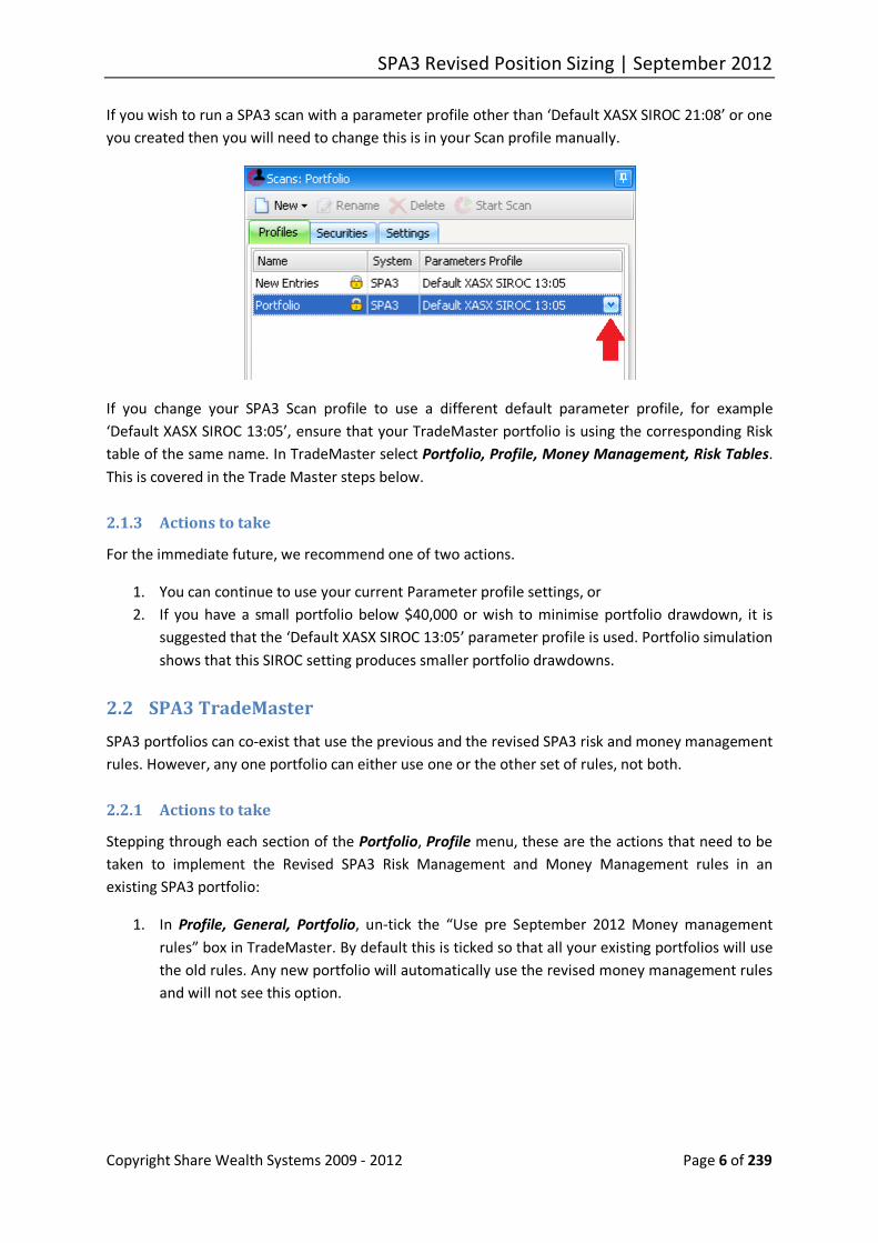
If you wish to run a SPA3 scan with a parameter profile other than ‘Default XASX SIROC 21:08’ or one you created then you will need to change this is in your Scan profile manually.
If you change your SPA3 Scan profile to use a different default parameter profile, for example ‘Default XASX SIROC 13:05’, ensure that your TradeMaster portfolio is using the corresponding Risk table of the same name. In TradeMaster select Portfolio, Profile, Money Management, Risk Tables. This is covered in the Trade Master steps below.
2.1.3 Actions to take
For the immediate future, we recommend one of two actions.
1. You can continue to use your current Parameter profile settings, or 2. If you have a small portfolio below $40,000 or wish to minimise portfolio drawdown, it is
suggested that the ‘Default XASX SIROC 13:05’ parameter profile is used. Portfolio simulation shows that this SIROC setting produces smaller portfolio drawdowns.
2.2 SPA3 TradeMaster
SPA3 portfolios can co-exist that use the previous and the revised SPA3 risk and money management rules. However, any one portfolio can either use one or the other set of rules, not both.
2.2.1 Actions to take
Stepping through each section of the Portfolio, Profile menu, these are the actions that need to be taken to implement the Revised SPA3 Risk Management and Money Management rules in an existing SPA3 portfolio:
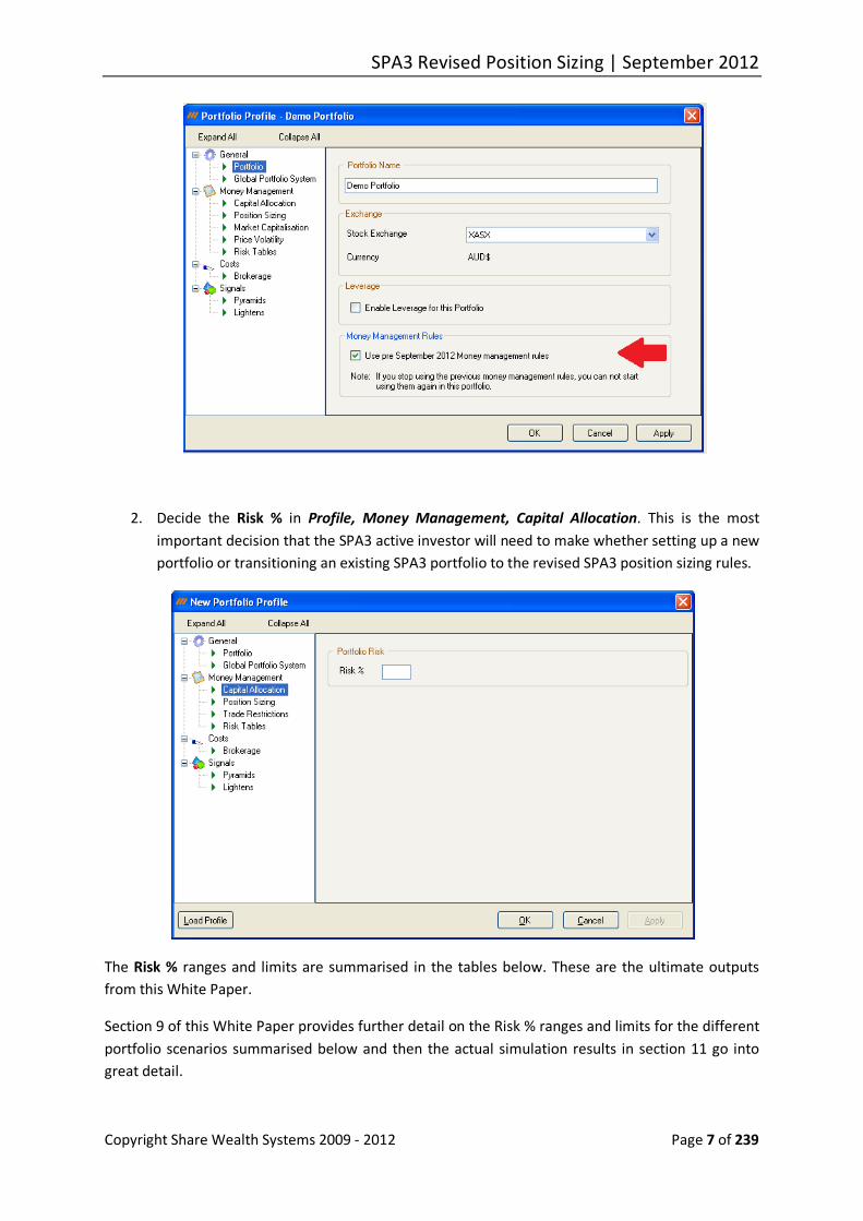
1. In Profile, General, Portfolio, un-tick the “Use pre September 2012 Money management rules” box in TradeMaster. By default this is ticked so that all your existing portfolios will use the old rules. Any new portfolio will automatically use the revised money management rules and will not see this option.
SPA3 Revised Position Sizing | September 2012
Copyright Share Wealth Systems 2009 - 2012 Page 7 of 239
2. Decide the Risk % in Profile, Money Management, Capital Allocation. This is the most important decision that the SPA3 active investor will need to make whether setting up a new portfolio or transitioning an existing SPA3 portfolio to the revised SPA3 position sizing rules.
The Risk % ranges and limits are summarised in the tables below. These are the ultimate outputs from this White Paper.
Section 9 of this White Paper provides further detail on the Risk % ranges and limits for the different portfolio scenarios summarised below and then the actual simulation results in section 11 go into great detail.

SPA3 Revised Position Sizing | September 2012
Copyright Share Wealth Systems 2009 - 2012 Page 8 of 239
It is recommended that a Risk % is selected in the range provided in the [Ideal] column. The start and end of the Ideal range are inclusive.
Portfolios using SIROC 21 8
$25,000 SIROC 21 8 8 Criteria Min
Risk % Ideal Max
Risk % Comments Chart Sections
Brokerage: $9.90, 0.1%, x5 Liq 0.5 0.6 – 1.5 1.5 11.2.2 Brokerage: $9.90, 0.1%, x10 Liq 0.5 0.8 – 1.2 1.5 11.2.3
$100,000 SIROC 21 8 8 Criteria Min
Risk % Ideal Max
Risk % Comments Chart Sections
Brokerage: $9.90, 0.1%, x5 Liq 0.3 0.5 – 0.8 1.0 11.2.5 Brokerage: $19.95, 0.1% 0.4 0.5 – 0.8 1.0 Not Simulated Brokerage: $27.50, 0.165%, x5 Liq 0.4 0.5 – 0.8 1.0 11.2.6
$400,000 SIROC 21 8 8 Criteria Min
Risk % Ideal Max
Risk % Comments Chart Sections
Brokerage: $27.50, 0.165%, x5 Liq 0.2 0.4 - 0.5 0.6 11.2.7 Brokerage: $19.95, 0.11% 0.2 0.4 - 0.5 0.6 Not simulated Brokerage: $9.90, 0.1% 0.2 0.4 – 0.5 0.7 Not simulated
Portfolios using SIROC 13 5 5
$25,000 SIROC 13 5 5 Criteria Min
Risk % Ideal Max
Risk % Comments Chart
Sections Brokerage: $27.50, 0.165% None None None Not recommended 11.3.2 Brokerage: $19.95, 0.1% 0.8 0.8 – 1.0 1.5 11.3.3 Brokerage: $9.90, 0.1% 0.4 0.8 – 1.2 1.5 11.3.4
$100,000 SIROC 13 5 5 Criteria Min
Risk % Ideal Max
Risk % Comments Chart Sections
Brokerage: $27.50, 0.165%, x5 Liq 0.3 0.4 – 0.8 1.0 11.3.6 Brokerage: $27.50, 0.165%, x10 Liq 0.3 0.4 – 0.8 1.0 11.3.7 Brokerage: $19.95, 0.1% 0.3 0.4 – 0.8 1.0 Not simulated Brokerage: $9.90, 0.1%, x5 Liq 0.2 0.3 – 0.5 1.0 11.3.8 Brokerage: $9.90, 0.1%, x10 Liq 0.2 0.4 – 0.6 1.0 11.3.9

SPA3 Revised Position Sizing | September 2012
Copyright Share Wealth Systems 2009 - 2012 Page 9 of 239
$$400,000 SIROC 13 5 5 Criteria Min
Risk % Ideal Max
Risk % Comments Chart Sections
Brokerage: $27.50, 0.165%, x5 Liq 0.2 0.4 – 0.5 0.6 11.3.10 Brokerage: $27.50, 0.165%, x10 Liq 0.2 0.4 – 0.5 0.6 11.3.11 Brokerage: $19.95, 0.1% 0.2 0.4 – 0.5 0.6 Not simulated Brokerage: $9.90, 0.1% 0.2 0.4 – 0.5 0.6 Not simulated
There is no wrong answer if a Risk % is selected in the ranges in the Ideal column above. If you wish to be far more specific then the portfolio simulation outcomes in section 11 should be consulted but initially this is not mandatory.
As a rule of thumb, if you wish to minimise drawdown then choose at the lower end, if you wish to maximise growth then choose at the higher end of the Ideal range but understand that larger position sizes are more sensitive to trading errors and to randomly selecting trades with poorer outcomes.
It is likely that you have a portfolio that is between the three starting values of $25,000, $100,000 and $400,000 chosen for simulation. A dose of common sense and erring towards a lower rather higher Risk % within the Ideal range should keep the SPA3 active investor on the straight and narrow. The Risk % can be changed at any time during the life of a portfolio.
3. Decide Market and Sector Risk settings in Profile, Money Management, Position Sizing.
The settings above will reflect the following risk management approach:
a. Risk Profile 1 - “When Market Risk is HIGH” reduces position sizes by 100%, i.e. no trade, for High and Low sector risk trades.
b. High Sector Risk trades will get a full position size because they are reduced by 0%. This is the setting that was used during all the simulations in this White Paper.

SPA3 Revised Position Sizing | September 2012
Copyright Share Wealth Systems 2009 - 2012 Page 10 of 239
Other settings can be selected. For example, if you wished to reduce the position size of a trade that has high sector risk, the bottom left quadrant should be changed to 33.33% of 50%, which ever you wish to reduce the position size by.
4. Decide the ATRVE volatility levels and minimum liquidity multiple that will be traded in Profile, Money Management, Trade Restrictions.
a. The default ATRVE levels of 1 to 12 that were used for the portfolio simulations in this paper are shown below.
b. To reduce portfolio equity curve volatility and hence potentially reduce drawdown the ATRVE levels could be narrowed down to, say, 1.5 – 2 for the minimum value and 4.5 – 5 for the maximum value. Refer to the December 2011 White Paper entitled “SPA3 Revived Edge” (which can be accessed from the GPS Help menu) for a detailed breakdown of the SPA3 raw edge by ATRVE volatility level.
c. The portfolio simulations used liquidity multiples or 5 and 10. A multiple in between can be used. A rule of thumb is that the smaller the portfolio value the higher liquidity multiple that can be used and the larger the portfolio the smaller the liquidity multiple should be but remember that the lower the multiple the bigger the liquidity risk that the active investor takes.
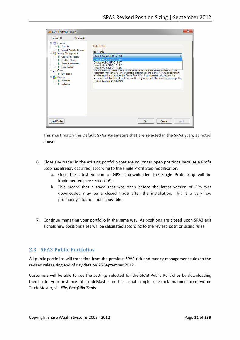
5. Select the SIROC default profile for your portfolio in Profile, Money Management, Risk Tables. Note the instructions in the Description box.
SPA3 Revised Position Sizing | September 2012
Copyright Share Wealth Systems 2009 - 2012 Page 11 of 239
This must match the Default SPA3 Parameters that are selected in the SPA3 Scan, as noted above.
6. Close any trades in the existing portfolio that are no longer open positions because a Profit Stop has already occurred, according to the single Profit Stop modification.
a. Once the latest version of GPS is downloaded the Single Profit Stop will be implemented (see section 16).
b. This means that a trade that was open before the latest version of GPS was downloaded may be a closed trade after the installation. This is a very low probability situation but is possible.
7. Continue managing your portfolio in the same way. As positions are closed upon SPA3 exit signals new positions sizes will be calculated according to the revised position sizing rules.
2.3 SPA3 Public Portfolios
All public portfolios will transition from the previous SPA3 risk and money management rules to the revised rules using end of day data on 26 September 2012.
Customers will be able to see the settings selected for the SPA3 Public Portfolios by downloading them into your instance of TradeMaster in the usual simple one-click manner from within TradeMaster, via File, Portfolio Tools.
SPA3 Revised Position Sizing | September 2012
Copyright Share Wealth Systems 2009 - 2012 Page 12 of 239
3 Objectives of the SPA3 Revision Project As SPA3 is an existing methodology, objectives had to be set for the revision project. These were set back in March 2011 and communicated to our customers in May 2011 via an eUGM, in the December 2011 White Paper and are repeated here.
The first and main objective was to improve performance. Improving performance has a number of inter-related objectives. In fact, all the objectives stated below, including the second and third objectives, lead to achieving this objective. The obvious performance measurements are:
• Increased returns, and
• Reduced drawdown.
These are achieved by improved timing, particularly exit signals, and by improved risk and money management.
The second objective was to improve the flexibility of SPA3 risk management and money management. This included:
• being able to start trading with the SPA3 methodology with starting capital as low as $10,000, and
• having a range of portfolio level risk management rules and associated money management rules that could support many and varied customised trader risk profiles from the very risk averse to the risky.
The third objective was to improve tradability. The aim is that it would become easier psychologically to trade with SPA3 regardless of previous trading experience or of the trader’s risk profile. This would be achieved through more sensitive exit signals and through greater flexibility with the risk management rules at the portfolio level, especially when first starting a portfolio.
We believe that all these objectives have been met, bar one that is met partially. Due to the mandatory cost of minimum brokerage we believe that actively trading a medium term methodology with as little as $10,000 with an unleveraged equities only strategy is not advisable. Whilst $20,000 or even $15,000 may just be OK for unleveraged equities trading with the position sizing model we have put forward in the paper with the minimum possible brokerage rate, as little as $10,000 may have to be left to the domain of leveraged trading to be able to make some headway without paying all the profits to a broker.
4 It all starts at the Trading Plan The content of a SPA3 trader’s Trading Plan is well documented in the SPA3 Getting Started Manual, the Education Centre in the SWS Members Zone and in the SPA3 Reference Manual.
The section of the Trading Plan that states the trader’s objectives is the Goals and Objectives Statement. This is the “what” section of the Trading Plan, what returns the active investor would like to achieve and within what risk constraints she / he would like to achieve these returns. There are three key areas of objectives:

SPA3 Revised Position Sizing | September 2012
Copyright Share Wealth Systems 2009 - 2012 Page 13 of 239
• Reward objectives. These are the periodic returns that a trader would like to achieve. Whilst actual returns achieved will depend on the performance of the market being traded, setting reward objectives helps determine the risk and money management rules that will be deployed. Also, if more than one methodology is being traded then setting reward objectives helps determine what instruments and markets should be traded and whether leverage should be used or not.
Your objective is more achievable if stated in terms of the market you are trading; for example, X% outperformance.
• Risk objectives. This is the maximum drawdown that one is prepared to endure in any single trading period. This could set parameters for when to reduce position sizes so as to remain within this drawdown objective or set a “shut-off” valve as to when to cease trading until the market returns to Low Risk or is once again in sync with your systems(s), as measured by a set of pre-determined researched criteria.
You may think that risk is related to the maximum amount of money you wish to lose. And it can be. You may put this in % terms.
But your benchmark should be your base reference. You are at the mercy of the market you are trading. For example, the All Ordinaries or the ASX200 or the ASX300; the
S&P500; the Nasdaq Composite or the Nasdaq 100.
You outperform the market by rising by more and by not falling as much.
• Skills objectives. This is a set of objectives to achieve skills-based targets with respect to mindset, trade execution, market environment understanding, trading understanding, journaling, practicing of trading and any other that you may wish to set. A schedule could be included here (or the next section of your Trading Plan) that details the books to be read, courses to attend, DVD’s to watch, Blogs to follow, internet research to be done, etc to achieve your skills objectives.
The inclusion of a risk objective is a key part of the SPA3 Trading Plan as this objective will be strongly tied to each individual’s choice and deployment of particular risk and money management rules in live trading.
5 Catch 22 – the major problem all investors face What position sizing approach a trader uses to trade is directly linked to the trader’s risk objective and reward objective that they state in their Trading Plan.
The Catch 22: how does a trader know in advance what position sizing approach to use to remain within their risk objective while also have a high probability of achieving their reward objective?
Answer: they don’t. Well, nearly every trader doesn’t.

SPA3 Revised Position Sizing | September 2012
Copyright Share Wealth Systems 2009 - 2012 Page 14 of 239
Stating a risk objective is easy enough, just state a number, like 20% maximum drawdown. Now what? Too large a position size will probably rush the trader to a maximum drawdown limit very quickly thereby taking the trader out of the opportunity flow that the market offers. Too small a position size might ensure that the maximum drawdown limit is never reached but also ensure that the reward objective is also never met.
How is this Catch 22 resolved? Using exploratory simulation. Let’s get into it.
6 Where to start the revision process? As discussed above in the Trading Plan section, ultimately the two main outcomes that a trader would like to control is the degree of risk (drawdown) and the degree of reward that they would like to achieve in their portfolio within the constraints of:
• How much capital they have to trade with. • How much time they have to devote to the trading process. • What their risk profile is, measured mainly by how much drawdown they can tolerate. • Their trading methodology (includes trading system, risk management and money
management). • The brokerage paid for each transaction relative to the individual position and potential
reward on offer, i.e. average return per trade. • The liquidity of the market that they trade relative to their trading capital. • The level of their trading psychology and skill.
We know that in any decent sized sample of active investors there will be a diverse range of maximum drawdown tolerance ranging from < 10% to as much as 60%. However, most of this same sample would use similar position sizes and risk management criteria in their trading, despite having very different methodologies and very different drawdown tolerance levels. This is so for two main reasons, because:
• most books contain similar suggestions about money management, e.g. the 2% and 6% rule, and
• there are very few sufficiently functional portfolio level risk and money management tools available and those few are priced above the range that the great majority would be prepared to pay for such functionality. Also, most retail investors wouldn’t have the knowledge to research to this level because it simply is not discussed in popular main stream books, i.e. we don’t know what we don’t know.
So if the two main outcomes that a trader needs to control is their level of portfolio drawdown and their portfolio returns, what is the main determinant that controls these two outcomes? The answer is: the risk and money management controls that are used for each individual trade and for their overall portfolio. The position size is THE biggest determinant of size of outcomes, both positively and negatively.
To be able to achieve one’s reward objectives whilst remaining within one’s risk objective constraints becomes the main balancing act that a trader needs to manage on an ongoing basis.

SPA3 Revised Position Sizing | September 2012
Copyright Share Wealth Systems 2009 - 2012 Page 15 of 239
This means that a trader requires as much flexibility as possible with their risk and money management rules to have the confidence to increase and reduce position sizes (even to $0) as required to increase returns without overstepping their stated risk objective, found in their Trading Plan Objectives Statement.
The degree of flexibility that a trader can have with their risk and money management rules is determined by the variation of individual trade outcomes. When combined with risk and money management rules, this leads to the degree of variation of potential portfolio equity curve outcomes, in terms of return AND drawdown. This is a key, possibly THE key statement in this paper. Due to its importance it is repeated here from the SWS December 2011 White Paper. Ensure that you grasp it. If not now, then return here when you have read the entire paper.
This means that the more similar each trade is to another the more flexibility a trader will have with their risk and position sizing rules which leads to a higher confidence level of achieving their anticipated portfolio outcome, as stated in their Trading Plan Objectives Statement.
Therefore, making each trade as similar as possible to each other becomes a trading system design objective, in order to reduce the variation of possible trade outcomes.
This was achieved with the SPA3 Revised Edge, as published and released in December 2011. The next major step in the research process is to conduct detailed historical portfolio exploratory simulation with different risk and money management criteria to determine which criteria work the best at the portfolio level with the particular edge, given a set of portfolio execution constraints such as portfolio capital, brokerage rates and market liquidity.
It is important to note that no one position size works well within all the constraints mentioned above, meaning that the best position size will be different for each set of constraints.
In seminars that I have delivered over the years it is amazing that traders’ with different trading approaches, trading different instruments with different amounts of leverage and different starting capitals mostly trade with the same position size, the 2% risk per trade model. Why? Probably because the ‘2% rule’ is regurgitated in book after book without the necessary research having been completed. This paper will make a mockery of this regurgitation.
Getting back to the degree of variation of potential portfolio equity curve outcomes, in terms of return AND drawdown, you should use this as one of the main criteria in determining how well the risk and money management rules fit the trading system, or edge, and how well the methodology (edge, risk management and money management) suit the given environment in which it executes.
Using this measurement will help you know when you can put a stake in the ground with your research and then move to executing in a live trading environment.
7 Research Environment The SWS December 2011 White Paper provided the outcomes from revising the SPA3 Edge. This White Paper now deals with the research process of matching risk and money management rules to

SPA3 Revised Position Sizing | September 2012
Copyright Share Wealth Systems 2009 - 2012 Page 16 of 239
the SPA3 Revised Edge and uses the universe of all trades that are generated from the SPA3 Revised Edge trading system entry and exit rules.
The SPA3 Revised Edge trades’ database is used as input to a portfolio level risk and money management engine that chronologically merges the following to create unique simulated equity curve values on a day by day basis:
1. Historical daily share price data. 2. Randomly chosen (other selection methods can be used) trades from the trades’ database
on any given trading day from all the trades signalled on that day, when a new trade is required to fill a portfolio position.
3. Portfolio risk rules and parameters to determine how much capital to expose to the chosen market.
4. Position sizes for individual new trades depending on risk rules. 5. Brokerage rates for entry and exit transactions. 6. Liquidity checks to ensure that illiquid trades relative to portfolio size are excluded from
execution.
Multiple hundreds or even multiple thousands of simulated equity curve numeric data are fed into a statistical programming environment (SWS uses R) which generates a number of equity curve statistics and portfolio straw-broom graphs.
Equity curve analysis is then conducted to determine a number of outcomes including:
• Variation of equity curves, the more similar the better.
Excel
Trades Database
Portfolio level Risk & Money Mgt
Engine
Stats Programming
e.g. ‘R’
Portfolio Equity Curve Analysis

SPA3 Revised Position Sizing | September 2012
Copyright Share Wealth Systems 2009 - 2012 Page 17 of 239
• Equity curve percentiles, e.g. 5, 25, 50 (median), 75 & 95 percentiles, of: o geometric mean, o maximum drawdown, o Win Rate & Profit Ratio, o number of trades, o unallocated equity (~ portfolio exposure), o Portfolio Performance Index (explained below), and o Downside Deviation Factor (explained below).
From this equity curve analysis other statistical metrics can be determined like the Geometric mean 5 percentile divided by the 95 percentile maximum drawdown. Depending on the values of these metrics the risk and position sizing rules can be changed and the process re-iterated. In fact, if the metrics are deemed substandard the entire process can be re-started going all the way back to the trading system concepts and rules.
8 Revised Risk Management and Money Management Rules in SPA3
8.1 Position Sizing calculation
In the prior SPA3 position sizing calculation the market capitalization, ATRVE (Volatility) at two levels - above and below 5% - and the SPA3 signal were used to determine whether a SPA3 trade was Low, Medium or High Risk. Effectively there were just three different position sizes for any given trade but there were also three sub-portfolios of capital.
If two SPA3 users had exactly the same portfolio value with the same number of open positions then their position size for a particular trade would have been exactly the same.
The previous portfolio construction rules required that a set number of open positions be selected prior to starting to trade. With the revised position sizing rules the number of simultaneously open positions is open-ended but limited by total portfolio capital and the position size.
Under the revised position sizing calculation, the Portfolio Risk % is the only input that a SPA3 user needs to decide on.
Position Size =Portfolio Value × Portfolio Risk %
Trade Risk %
Portfolio Risk %: Percentage of the Portfolio Value you are willing to risk (lose) on a trade.
Trade Risk %: Amount of risk (loss) that may occur in this trade. This is the ‘expected loss’ but can also be the distance to a trailing stop for each particular trade.
To determine the Trade Risk % for any trade we use the volatility level (ATRVE) and the SPA3 signal. From quantitative analysis of thousands of historical trades, we found that the combination of these two characteristics provide the primary determinates of the ‘expected loss’ of a trade. This combination replaces the previous SPA3 Risk Tables. Notable changes are:
SPA3 Revised Position Sizing | September 2012
Copyright Share Wealth Systems 2009 - 2012 Page 18 of 239
• The new Trade Risk % has no discrete levels. A change in the ATRVE value will result in a smooth and relative change in the Trade Risk %.
• There are ranges of ATRVE values for each SPA3 signal that will be designated as a ‘No Trade’.
The expected Trade Risk %’s are stored in TradeMaster and used in the position size calculation
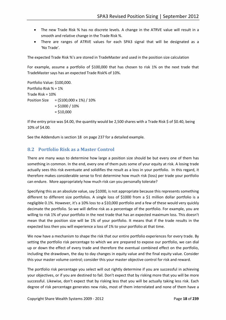
For example, assume a portfolio of $100,000 that has chosen to risk 1% on the next trade that TradeMaster says has an expected Trade Risk% of 10%.
Portfolio Value: $100,000. Portfolio Risk % = 1% Trade Risk = 10% Position Size = ($100,000 x 1%) / 10% = $1000 / 10% = $10,000
If the entry price was $4.00, the quantity would be 2,500 shares with a Trade Risk $ of $0.40, being 10% of $4.00.
See the Addendum is section 18 on page 237 for a detailed example.
8.2 Portfolio Risk as a Master Control
There are many ways to determine how large a position size should be but every one of them has something in common. In the end, every one of them puts some of your equity at risk. A losing trade actually sees this risk eventuate and solidifies the result as a loss in your portfolio. In this regard, it therefore makes considerable sense to first determine how much risk (loss) per trade your portfolio can endure. More appropriately how much risk can you personally tolerate?
Specifying this as an absolute value, say $1000, is not appropriate because this represents something different to different size portfolios. A single loss of $1000 from a $1 million dollar portfolio is a negligible 0.1%. However, it’s a 10% loss to a $10,000 portfolio and a few of these would very quickly decimate the portfolio. So we will define risk as a percentage of the portfolio. For example, you are willing to risk 1% of your portfolio in the next trade that has an expected maximum loss. This doesn’t mean that the position size will be 1% of your portfolio. It means that if the trade results in the expected loss then you will experience a loss of 1% to your portfolio at that time.
We now have a mechanism to shape the risk that our entire portfolio experiences for every trade. By setting the portfolio risk percentage to which we are prepared to expose our portfolio, we can dial up or down the effect of every trade and therefore the eventual combined effect on the portfolio, including the drawdown, the day to day changes in equity value and the final equity value. Consider this your master volume control; consider this your master objective control for risk and reward.
The portfolio risk percentage you select will out rightly determine if you are successful in achieving your objectives, or if you are destined to fail. Don’t expect that by risking more that you will be more successful. Likewise, don’t expect that by risking less that you will be actually taking less risk. Each degree of risk percentage generates new risks, most of them interrelated and none of them have a

SPA3 Revised Position Sizing | September 2012
Copyright Share Wealth Systems 2009 - 2012 Page 19 of 239
perfect solution. The best possible solution we can aim for is one that minimises all risks to an acceptable level. This is no easy task. Every trader has a different risk tolerance, every portfolio has a different value, and market conditions will continue to vary.
Therefore, the only variable in the above position sizing calculation that the SPA3 trader needs to decide is the Portfolio Risk %, or % Risk per Trade as it is also known. How does one know what the correct Portfolio Risk % or % Risk per Trade is for their set of trading circumstances taking into account portfolio size, brokerage rates, personal risk profile, drawdown risk objective, reward risk objective etc? Should it be 1%, or 2% as most books regurgitate, or 0.5% or 3% or 0.87%?
Rather than trading blindly with a guessed % Risk Per Trade and then letting one’s live trading results tell you over a large sample of trades whether you are taking too much or too little risk (which may take many months or even years), we use exploratory simulation to get the answers before we start trading.
9 Portfolio Limits and Boundaries This section provides the range of SWS suggested position sizes based on the analysis of the exploratory simulation research. The ‘Default XASX Profile’ SPA3 parameters were used to generate the trades’ database that was used for the respective simulations.
9.1 Different SIROC parameters
From a SPA3 Revised Edge perspective, the following SIROC parameters were re-researched since the December 2011 White Paper with the single Profit Stop (see Section 16 below), where the third parameter is the daily SIROC EMA setting:
• SIROC 5 3 5 • SIROC 8 3 5 • SIROC 13 5 5 • SIROC 17 7 8 • SIROC 19 7 8 • SIROC 21 8 8 • SIROC 26 9 8 • SIROC 30 10 8 • SIROC 34 13 8 • SIROC 55 21 8
Fig 9.1 shows the Expectancy and SQN (System Quality Number – see the December 2011 White Paper) for all trades with each of the SIROC settings above on the horizontal axis. The distribution curve shows that, using the SQN, the SIROC 17 7 8 is a tiny bit better than the other SIROC settings as it is at the top of the curve. SIROC 19 7 then SIROC 13 5 5 then SIROC 21 8 are close behind.

SPA3 Revised Position Sizing | September 2012
Copyright Share Wealth Systems 2009 - 2012 Page 20 of 239
Fig 9.1
Only two sets of SIROC parameter settings were researched using exploratory simulation, the SIROC 21 8 8 and SIROC 13 5 5. However SPA3 users can quite safely use SIROC 17 7 8 and SIROC 19 7 8 as well, as can any other either SIROC settings, but any of these four are recommended. The Trade Risk % risk tables are programmed into TradeMaster for all four SIROC settings.
For each of the two SIROC settings, SIROC 21 8 8 and SIROC 13 5 5, that were simulated, three portfolio starting capital amounts were researched, $25,000, $100,000 and $400,000. Three different brokerage rates were also researched and different liquidity settings. A number of different Portfolio Risk % settings were researched to calculate position size, ranging from 0.2% to 3%.
9.2 An introduction to Box Plots
The simplicity of the box plot makes it ideal as a means of visually comparing large sets of data. Box plots of a group of portfolio tests can be lined up side by side and the various attributes of the portfolios compared at a glance. Obvious changes in values and ranges are immediately apparent.
The box segment represents the range of values produced by the central 50% of portfolios. That is 25% of portfolios produced values below the box and 25% of portfolios produced values above the box. The vertical ‘T’ lines are known as whiskers. Throughout this paper, the upper whisker, labelled ‘MAXIMUM’ represents the values at the 5th percentile of portfolios. That is, there were another 5% of portfolios that produced values greater than the top whisker. The lower whisker, labelled

SPA3 Revised Position Sizing | September 2012
Copyright Share Wealth Systems 2009 - 2012 Page 21 of 239
‘MINIMUM’ represents the values at the 95th percentile of portfolios. That is, there were another 5% of portfolios that produced values less than the lower whisker.
9.3 Portfolio Limits using SIROC 21 8
This section provides Portfolio Risk % boundaries for portfolios that use the SIROC 21 8 8 parameter settings, all other SPA3 settings being as per the SPA3 Revised Edge for the ASX with a single Profit Stop.
HINT: View the ‘box charts’ and simulated portfolio equity curves alongside each of the tables below, so as to compare and follow the reasoning behind the
suggested limits and boundaries. The commentary below will also make more sense.
9.3.1 $25,000 Portfolios
$25,000 SIROC 21 8 8 Criteria Min
Risk % Ideal Max
Risk % Comments Chart Sections
No Liquidity Check, $9.90, 0.1% 0.4 2.5 Not recommended 11.2.1 Brokerage: $9.90, 0.1%, x5 Liq 0.5 0.6 – 1.5 1.5 11.2.2 Brokerage: $9.90, 0.1%, x10 Liq 0.5 0.8 – 1.2 1.5 11.2.3
9.3.1.1 Comments
Whilst it makes good sense to minimise brokerage rates with any active investment strategy, with small starting capital bases of $20,000 to $40,000 it is mandatory. Hence we have simulated just the $9.90 or 0.1%, whichever is the larger, brokerage rate for the SIROC 21 8 setting on a $25,000 portfolio. Using a larger brokerage rate would have similar effects with the SIROC 21 8 as it has with the SIROC 13 5 5 settings shown above. Brokerage rates of $27.50 or 0.165% and %19.95 or 0.1% are

SPA3 Revised Position Sizing | September 2012
Copyright Share Wealth Systems 2009 - 2012 Page 22 of 239
simulated with the SIROC 13 5 5 parameter settings to show that the $27.50 / 0.165% combination should NOT be used with a small portfolio.
The higher liquidity requirement of x10 compared to x5 does curtail performance a little in that the potential to perform better with a larger position size is reduced. Notice in sections 11.2.2 and 11.2.3 how using 1.5% Risk %, the Portfolio Performance Index (PPI) box plot starts falling for the x10 liquidity at 1.5% and the upper quartile of the box plot of the Geometric Mean is lower compared to the x5 liquidity.
Which position size to use in the ‘ideal’ ranges provided above will depend on what the Objectives are that have been set in your Trading Plan Goals & Objectives Statement.
For example, for a 1.5% Risk % with x5 liquidity the PPI and Geometric Mean 5% and 25% percentiles at the top of the box plots are higher than for position sizes with Risk % of 0.8% - approx. 0.12%. However, the 95% and 75% are lower meaning that the worse portfolio outcomes for a 1.5% Risk % will be worse than for the 0.8% - 1.2% Risk % portfolios.
The simulated portfolio outcomes have selected SPA3 trades on a random basis. Therefore if you trust yourself that will not make trading errors and that your trade selection will be better than the average of a random trade selection process then using the larger position size in the range of 0.8% - 1.2% can provide you with a better return that a smaller position size.
If you trade with a higher brokerage rate than $9.90 or 0.1% then you will have to err towards the lower end of the [Ideal] range of Risk % choice. Refer to the SIROC 13 5 5 simulated results below for further insight.
9.3.2 $100,000 Portfolios
$100,000 SIROC 21 8 8 Criteria Min
Risk % Ideal Max
Risk % Comments Chart Sections
No Liquidity Check, $27.50, 0.165% 0.3 2.0 Not recommended 11.2.4 Brokerage: $9.90, 0.1%, x5 Liq 0.3 0.5 – 0.8 1.0 11.2.5 Brokerage: $19.95, 0.1% 0.4 0.5 – 0.8 1.0 Not Simulated Brokerage: $27.50, 0.165%, x5 Liq 0.4 0.5 – 0.8 1.0 11.2.6
9.3.2.1 Comments
$100,000 portfolios are still affected by the higher $27.50 / 0.165% brokerage rate but nowhere near as much as a smaller portfolio i the $20,000 - $40,000 range.

SPA3 Revised Position Sizing | September 2012
Copyright Share Wealth Systems 2009 - 2012 Page 23 of 239
9.3.3 $400,000 Portfolios
$400,000 SIROC 21 8 8 Criteria Min
Risk % Ideal Max
Risk % Comments Chart Sections
Brokerage: $27.50, 0.165%, x5 Liq 0.2 0.4 - 0.5 0.6 11.2.7 Brokerage: $19.95, 0.11% 0.2 0.4- 0.5 0.6 Not simulated Brokerage: $9.90, 0.1% 0.2 0.4 – 0.5 0.7 Not simulated
9.3.3.1 Comments
Larger portfolios can sustain higher brokerage levels much better than smaller portfolios.
However, larger portfolios suffer lower comparative growth, as measured by geometric mean in the simulations results in this paper, due mainly to the lack of liquidity in the overall Australian equities market. However, outperformance of the All Ordinaries index is still quite spectacular over the sample research period.
Hence Risk % has to be smaller in larger portfolios due to this liquidity issue. Whilst a small 0.2% Risk % wouldn’t be too affected by the higher brokerage level the issue becomes the absolute number of trades that SPA3 traders would need to complete. Positively though, SPA3 continues to provide sufficient opportunity to trade if traders are happy to be that active. Simultaneously open position charts are provided in the detailed sections of the paper.
9.4 Portfolio Limits using SIROC 13 5 5 – Close immediately
This section provides Portfolio Risk % boundaries for portfolios that use the SIROC 13 5 5 parameter settings, all other SPA3 settings being as per the SPA3 Revised Edge for the ASX with a single Profit Stop. Trades are closed immediately when the Market Risk turns to High Risk.
HINT: View the ‘box charts’ and simulated portfolio equity curves alongside each of the tables below, so as to compare and follow the reasoning behind the
suggested limits and boundaries.
9.4.1 $25,000 Portfolios
$25,000 SIROC 13 5 5 Criteria Min
Risk % Ideal Max
Risk % Comments Chart
Sections No Liquidity Check None Not recommended 11.3.1 Brokerage: $27.50, 0.165% None None None Not recommended 11.3.2 Brokerage: $19.95, 0.1% 0.8 0.8 – 1.0 1.5 11.3.3 Brokerage: $9.90, 0.1% 0.4 0.8 – 1.2 1.5 11.3.4

SPA3 Revised Position Sizing | September 2012
Copyright Share Wealth Systems 2009 - 2012 Page 24 of 239
9.4.1.1 Comments
Whilst the Max Risk % in the table above shows 1.5%, the maximum Risk % which should be traded is 2, due to Volatility Drag (this is explained in the Appendix). Beyond a Risk % of 2 the variation of portfolio outcomes starts to widen and fall quickly.
A small portfolio is highly susceptible to meltdown from high brokerage rates. As the brokerage rate increases the minimum Risk % with which to calculate position sizes needs to rise accordingly. For lower brokerage rates, the range of [Ideal] Risk % with which to calculate position sizes widens thereby increasing the trader’s position size flexibility and the probability of outperformance whilst reducing the risk of underperformance.
This is primarily due to:
1. Less capital being directed towards the broker and more capital being put to work in the market for the active investor.
2. The increased number of trades that flow through the portfolio which contributes directly to compounding. The additional trades include those with greater Trade Risk, from increased volatility, which typically come with greater reward, provided risk is managed by sticking to the SPA3 rules.
The availability of trades is not an issue.
Liquidity has a minor effect on smaller portfolios because the absolute size of positions is small.
9.4.2 $100,000 Portfolios
$100,000 SIROC 13 5 5 Criteria Min
Risk % Ideal Max
Risk % Comments Chart Sections
No Liquidity Check None Not recommended 11.3.5 Brokerage: $27.50, 0.165%, x5 Liq 0.3 0.4 – 0.8 1.0 11.3.6 Brokerage: $27.50, 0.165%, x10 Liq 0.3 0.4 – 0.8 1.0 11.3.7 Brokerage: $19.95, 0.1%, x10 Liq 0.3 0.4 – 0.8 1.0 Not simulated Brokerage: $9.90, 0.1%, x5 Liq 0.2 0.3 – 0.5 1.0 11.3.8 Brokerage: $9.90, 0.1%, x10 Liq 0.2 0.4 – 0.6 1.0 11.3.9
9.4.2.1 Comments
A medium sized portfolio is starting to see significant easing of the meltdown from brokerage issues. The smaller brokerages still restrict the minimum Risk % possible but increasing the brokerage does not increase the minimum Risk % accordingly. The ideal Risk % values are now considerably lower.
The reason that the [Ideal] range narrows for the lower brokerage level of $9.90 / 0.1% is that these Risk % selections stand out as far better when the brokerage level is reduced. At the higher brokerage level there is not as much difference between the Risk %
The maximum Risk % which should be traded due to Volatility Drag is 1. Even at this point the range of portfolio equity curves has started to widen and fall quickly to unnecessarily low levels. Trading
SPA3 Revised Position Sizing | September 2012
Copyright Share Wealth Systems 2009 - 2012 Page 25 of 239
these higher Risk % values would only be done to reduce the trade frequency or reduce the effect of larger brokerage.
Medium sized portfolios will start to see impact from insufficient liquidity as the portfolios grow.
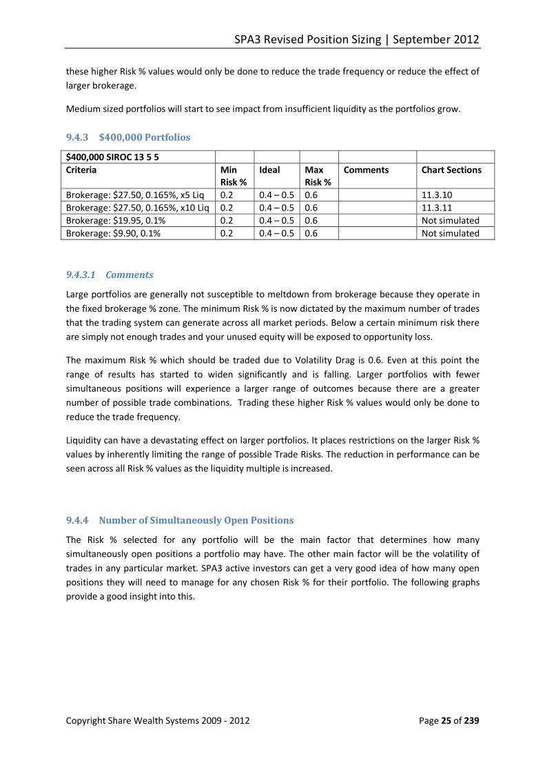
9.4.3 $400,000 Portfolios
$400,000 SIROC 13 5 5 Criteria Min
Risk % Ideal Max
Risk % Comments Chart Sections
Brokerage: $27.50, 0.165%, x5 Liq 0.2 0.4 – 0.5 0.6 11.3.10 Brokerage: $27.50, 0.165%, x10 Liq 0.2 0.4 – 0.5 0.6 11.3.11 Brokerage: $19.95, 0.1% 0.2 0.4 – 0.5 0.6 Not simulated Brokerage: $9.90, 0.1% 0.2 0.4 – 0.5 0.6 Not simulated
9.4.3.1 Comments
Large portfolios are generally not susceptible to meltdown from brokerage because they operate in the fixed brokerage % zone. The minimum Risk % is now dictated by the maximum number of trades that the trading system can generate across all market periods. Below a certain minimum risk there are simply not enough trades and your unused equity will be exposed to opportunity loss.
The maximum Risk % which should be traded due to Volatility Drag is 0.6. Even at this point the range of results has started to widen significantly and is falling. Larger portfolios with fewer simultaneous positions will experience a larger range of outcomes because there are a greater number of possible trade combinations. Trading these higher Risk % values would only be done to reduce the trade frequency.
Liquidity can have a devastating effect on larger portfolios. It places restrictions on the larger Risk % values by inherently limiting the range of possible Trade Risks. The reduction in performance can be seen across all Risk % values as the liquidity multiple is increased.
9.4.4 Number of Simultaneously Open Positions
The Risk % selected for any portfolio will be the main factor that determines how many simultaneously open positions a portfolio may have. The other main factor will be the volatility of trades in any particular market. SPA3 active investors can get a very good idea of how many open positions they will need to manage for any chosen Risk % for their portfolio. The following graphs provide a good insight into this.

SPA3 Revised Position Sizing | September 2012
Copyright Share Wealth Systems 2009 - 2012 Page 26 of 239
The Open Positions charts above show the number of simultaneous open positions for a 0.2%, 0.3%, 0.4%, 0.5%, 0.6% and 0.8% Portfolio Risk % on the ASX. 0.2% and 0.3% will be a comparatively high number of positions to manage for most private active investors. 0.4% may still be a little on the high side but the risk to reward at this Risk % may make it worthwhile for some portfolio scenarios depending on starting capital and brokerage. Risk %’s of 0.5% - 0.8% should be just fine.
The following two graphs show the number of simultaneously open positions from simulating trading SPA3 on the NASDAQ with Risk % of 0.6% and 0.8%. Compare these to the corresponding Risk % for the ASX. Besides periods of volatility the number of simultaneously open positions is very similar.

SPA3 Revised Position Sizing | September 2012
Copyright Share Wealth Systems 2009 - 2012 Page 27 of 239
The following two graphs show the number of simultaneously open positions from simulating trading SPA3 on the ASX and NASDAQ, respectively, with Risk % of 1.0%.
Using a Risk% of 1.5% will reduce the number of open positions to an average of around 8 - 9 and of 2.0% to an average of 6 - 7.
This section is provided here to assist SPA3 active investors with selecting the Risk % for their portfolio.
10 Exploratory Simulation
10.1 Introduction
Please refer to the December 2011 White Paper for an introduction to exploratory simulation.
Exploratory simulation can only start once a mechanical system with an edge is established that has generated sufficient historical trades from which to compile historically simulated portfolios against past stock data.
Our main purpose here is to determine a suitable position size for a given set of trading circumstances and ultimately determine the chances of a trader achieving their reward and risk objectives in their Trading Plan.

SPA3 Revised Position Sizing | September 2012
Copyright Share Wealth Systems 2009 - 2012 Page 28 of 239
To achieve this, a back test needs to be run that simulates the mechanical process of operating a portfolio using the exact criteria that will be used in live trading. The problem with a back test is that only a single portfolio is created using a subset of the whole universe of possible historical trades and is therefore only one unique sample of what could have happened.
The different choices that each investor makes at any decision point will set them upon a different unique path to every other investor; each will have a different outcome to their portfolio and each will have a unique mix of historical trades that would have been executed in their portfolio.
These choices include; portfolio size, trade selection, trading system settings, stock liquidity requirements, brokerage rates and money management settings. All of these will produce thousands and thousands of different permutations over an extended period of time. So you can’t just run one back test, you need to run thousands.
Traditional simulation and software simulation tools would use Monte Carlo analysis. In brief, with Monte Carlo all the trades from the entire trade period are thrown into one bucket and then randomly drawn to create an imaginary portfolio. Monte Carlo analysis jumbles time randomly and therefore ignores any dependencies between trades that might have occurred such as during strong market downturns and run-ups, i.e. during strong trending periods.
Although the Monte Carlo process has some value, in that it will simulate an ‘edge’ according to its statistical expectancy, it has one major flaw that precluded us from using it. It is effectively incapable of simulating the true effect that market sentiment has on a portfolio of multiple positions in multiple securities with dependency. Consequently, Monte Carlo underestimates the actual risks from real market events, like the 2008 ‘financial crisis’, and prevents the proper portfolio simulation of money management and its outcomes by under-simulating maximum drawdowns in such market conditions. Monte Carlo would be more useful in single position simulations, such as just a Gold portfolio or just an S&P500 futures portfolio, than for portfolios with multiple simultaneously open positions such as an equities portfolio.
What we needed was a test technique that created simulated portfolios using the exact trading conditions that were available during the test period. This includes the exact order and timing of trade signals, market conditions, trading costs and money management rules. This is the only way to know what might have happened for you and, hence, gain a very good idea of what may happen in the future. We found this in a technique called Exploratory Simulation.
The result is a range of portfolio equity curves that cover a statistically significant sample of possible outcomes over the test period. We found that 1000 simulated portfolios were needed to provide a statistically significant sample that would be representative of possible portfolio scenarios over a > 10 year period. Would this cover EVERY possible scenario? Well, no. That’s what statistical analysis does, it uses a sample that is deemed statistically significant to be representative of the entire possible universe of outcomes and then attaches probabilities to the potential for the statistical sample to repeat in the future. Perfection and dead certainties will never be achieved but such statistical analysis has major advantages over not doing the research and statistical analysis at all. Mechanical trading is the execution of a process that is heavily based on statistical probabilities, nothing more nothing less.

SPA3 Revised Position Sizing | September 2012
Copyright Share Wealth Systems 2009 - 2012 Page 29 of 239
Every exploratory simulation run produces an equity curve and trade statistics. The combined data from 1000 runs generate a powerful picture of the range of portfolio behaviour given a set of risk and money management rules. Your capability of thriving and surviving is immediately evident. The impact of your trading environment and every decision or change to a process is shown clearly.
Exploratory Simulation allows you to know if your objectives are achievable with a far higher degree of certainty than with not using exploratory simulation.
10.2 Extent of exploratory simulation research
This has been a huge project no matter which way you measure the effort and the resource that has been committed to it. At times it seemed that it would be never ending! As I have said many times before, having a loyal customer base to which a commitment such as this can be made is a major motivation to keep on keeping on and to eventually deliver.
Detailed research for this project started in June 2011. Well over 500,000 portfolio simulations have been run in this project. Well over 2,500 dedicated man hours have been invested in this revision project of SPA3 risk and money management.
The specialised software tools used in the project are complex and require a detailed level of computer skills and C++ programming skills. The peripheral tools required for statistical analysis, such as R and Excel, are also used at intricate levels. This of course excludes the pre-requisite financial markets and trading knowledge required to embark on such a project.
In the exploratory simulations conducted and the results of which are provided in this paper the following criteria were used:
• ASX only trades from 4/1/2000 (first trading day of the century) to 31/1/2012. • All listed and delisted ASX stocks during this period. This means that a stock that was
delisted after January 2000 and before December 2011 will be included in the simulations. • An open-ended number of simultaneously open positions per portfolio. • Randomly chosen trade selection from available trades whenever there was available capital
to be invested, according to Risk Profile 1. o This means that on any given day where there was more than one SPA3 trade
available to select from, the trade was chosen on a purely random basis, provided the trade was liquid enough. If not, then the next trade that was liquid enough was selected randomly.
o If there was insufficient capital available to fill a required position size then the position size was NOT reduced to fill the position. This means that there are times through the life of the simulations that portfolios were not fully invested. You may devise a set of common sense rules for your own Trading Plans
whereby you reduce the position size to appoint but no less to make the trade with a smaller position size.
• The Portfolio Risk % for new position sizes were not decreased or increased for each simulation, they remained the same, based on the position size calculation, throughout the research period.
• No pyramiding or lightening was used.
SPA3 Revised Position Sizing | September 2012
Copyright Share Wealth Systems 2009 - 2012 Page 30 of 239
• Risk Profile 1 was used in all simulations, that is portfolios were moved 100% into cash when a SPA3 High Market Risk occurred.
• During Low Market Risk, all High Sector Risk trades were allocated a full position, that is, there was no reduction in position size for Sector Risk.
• In sections 11.2 (SIROC 21 8) and 11.3 (SIROC 13 5 5) all positions were closed immediately on the trading day after a SPA3 High Market Risk signal occurred.
• In section 11.4 some equity curves for the SIROC 13 5 5 allowed trades to exit normally when a SPA3 High Market Risk occurred with no new positions taken. These are noted accordingly.
• Simulations included brokerage as shown. • No dividends or interest have been included in the equity curves. The additional returns that
would be generated from these two sources would be substantial in absolute terms and in compounding terms over a period of 12 years.
• No tax is included in the equity curves except for brokerage GST.
Each historical portfolio equity curve is an unrealized profit equity curve or a mark-to-market equity curve with the portfolio value being recalculated on a daily basis for the life of the portfolio.
10.3 Research period
Some comment on the research period that has been used for the portfolio simulation is required.
Big picture technical analysis will show that a secular bear market in equities started on the $DJI in January 2000 and in March 2000 on the NASDAQ Composite and S&P500. On the ASX a case might be argued against a secular bear market starting at this time as a major new high well above the March 2000 high was made in 2007. However, the period chosen has the following traits:
• Two major bear markets in the ALL ORDS of 20% and 54%. These might be termed primary bear markets within a secular bear market.
• Major geopolitical events in September 2001 in New York and July 2007 in London. • Major natural disaster events such as the tsunami in Japan in March 2011. • Primary bull markets within the secular bear market such from March 2003 and March 2009.
This is a fantastic sample research period with which to conduct exploratory simulation to demonstrate robustness of a methodology’s timing, risk management and position sizing rules.
However, the benchmark index of the market that we have researched still had an upwards bias. The ALL ORDS rose by around 30% over this period. That said the advance decline line for the ALL ORDS had a downward bias meaning that far more stocks fell than rose over this period.
In another paper due out later this year we will demonstrate SPA3 outperforming the NASDAQ Composite over the same sample period of January 2000 – January 2012. Over this period the NASDAQ Composite had a downward bias, falling 30% over this period with 2 x major primary bear markets and one major primary bull market during the secular bear market.
It is not secular bull markets such as 1982 to January 2000 that investors need worry about, it is secular bear markets such as we have experienced since 2000 and such as 1966 to 1982 that

SPA3 Revised Position Sizing | September 2012
Copyright Share Wealth Systems 2009 - 2012 Page 31 of 239
investors must prepare themselves for. If your strategy can make positive headway during such periods then handling the secular bull market will be a fantastic ride.
As mentioned above, all the exploratory simulations conducted in this paper have been done with SPA3’s Risk Profile 1 risk management approach. This begs the question, is using Risk Profile 2 still a valid risk management approach? It is our considered view that it is, but probably only during secular bull markets. Another research project ……….
11 Exploratory Simulation Outcomes
11.1 Introduction
This section will show the graphical outcomes from this round of SPA3 research.
The main purpose of this section is to provide graphical output to support SPA3 users choosing what position size to use for their own respective investing scenarios.
Whilst there may seem to be plenty of pages, not all pages are relevant to everybody. The detail has been provided so that each SPA3 user can hone in on a portfolio scenario that is relevant to them. Of course, perusing all the material can be of great educational value. In the future we will investigate providing access to this information via a tool of sorts.
The other purposes of this section are to:
1. take the reader through a process of gaining understanding of what steps were taken to revise the SPA3 Money Management rules according to the objectives set for the research project,
2. understand why the SPA3 Revised Money Management rules are an improvement on the previous money management rules,
3. understand how extremely important it is to get one’s position sizing correct in harmony with their system and execution environment, and
4. importantly, build belief and trust in the methodology such that it is executed with consistency and confidence to be able to grow one’s trading capital to reach ones financial objectives.
Only the ASX research results are provided at this stage for unleveraged trading. JSE research results and the NASDAQ research results will be provided in future papers, as will leveraged trading with CFDs.
Each set of charts will be headed according to the following portfolio variables:
1. The amount of starting capital as at 4/1/2000, the first trading day of 2000. 2. The SIROC parameters used. 3. The liquidity check to ensure that there was sufficient liquidity to take the trade. 4. The brokerage rate used for the life of the simulation.
Two types of graphs will be shown for each portfolio scenario, straw-broom graphs and box plots.

SPA3 Revised Position Sizing | September 2012
Copyright Share Wealth Systems 2009 - 2012 Page 32 of 239
Each of the straw-broom charts show 1000 unique simulated portfolio equity curves. Each straw-broom chart has been back-tested with a different position size. Each equity curve has a unique mix of SPA3 trades that have been selected randomly based on meeting the liquidity check for the simulation. This statement applies to all the straw-broom charts that are in this White Paper.
A quick scan of the straw-broom graphs will help reveal the better Portfolio Risk %’s to use for each portfolio scenario. Notes are provided for most of the portfolio scenarios.
The box plots that are provided for each scenario show the following measurements:
1. Portfolio Performance Index.
Investors frequently associate risk with failure to attain a target return. The target is typically the return offered by a benchmark such as the relevant market index. For funds invested in the Australian stock market the common benchmark is the All Ordinaries Index ($XAO) or the S&P/ASX 200 Index ($XJO). Such benchmark comparisons are widespread in the investment industry, along with a fear of underperforming them. Benchmarks offer a fixed point of reference against which different market investments can be measured, in particular the expected return.
An investor expects that over a period of time that their portfolio will outperform the benchmark returns. As time passes the probability that a portfolio WILL outperform the benchmark is increased by having returns:
• that are more frequently greater than the benchmark, and • that are larger than the benchmark, including small losses.
“The Portfolio Performance Index (PPI) takes both of these into account to generate a number that measures a portfolios likelihood of outperforming the benchmark.”
This measurement can be used to rank several portfolios alongside each other. The benefits of this form of outperformance measurement are:
• The comparison can take place regardless of the starting capital of each portfolio. • Continuous outperformance over the period is ranked above short periods of large
outperformance, which create the false perception of overall outperformance. • The returns do not have to adhere to a normal statistical distribution, which would
typically interfere with the result.
2. Downside Deviation Factor
It would be generally agreed that when a portfolio has loss trades, it’s best if they aren’t too big and don’t occur too often. This statement suggests there should be two dimensions to any risk measurement; magnitude and probability. The common risk measurement of Average Loss % provides the dimension of magnitude but not probability. An alternative measurement is Downside Deviation (DSD) which measures the variation of returns below a
SPA3 Revised Position Sizing | September 2012
Copyright Share Wealth Systems 2009 - 2012 Page 33 of 239
target return. The result is a value that not only provides the dimension of magnitude in a statistical manner but also includes the second dimension, the probability of Loss.
An investor expects that over a period of time that the risk, in the form of loses, experienced by their portfolio will be less than that of the benchmark. The perceived risk is loosely assessed by the investor in terms of the actual magnitude and frequency experienced, against the benchmark. The Downside Deviation Factor (DDF) is a measurement that allows the risk experienced by several portfolios to be accurately compared against that presented by a benchmark.
The DDF, takes the Downside Deviation (DSD) for a portfolio and compares it directly against the DSD for the chosen benchmark.
“The DDF represents how much more or less risk, by a factor, a portfolio presents compared to the benchmark.”
The DDF ranges between 0 and 2, with a factor of 1 meaning that the portfolio offers the same risk as the benchmark. A factor below 1 means that the portfolio offers less risk, and a factor greater than 1 means that it offers more risk.
(Note, the DDF range is not linear so don’t interpret a DDF of 2 as twice as much risk. In fact it’s a lot more than that!)
3. Daily Geometric Mean. This the single daily growth factor for the entire life of the simulated portfolios. Use this to determine the best performing position size for any given portfolio scenario. The higher the better but it must be analysed in conjunction with the Portfolio Performance Index and Downside Deviation Factor.
4. Maximum Drawdown %. This is the single maximum drawdown that each of the unique portfolios reached during the life of that portfolio. All other drawdown levels would have been less than the maximum drawdown for the life of the portfolio. In some instances underwater equity curves have been included to provide an insight into the nature of drawdowns throughout the life of the portfolio in comparison to the single maximum drawdown.
5. Unallocated Equity Deviation. A reading of 30% means that the portfolio was unallocated for 30% of the life of the portfolio which means that it was 70% allocated. Remember that all the simulations used SPA3 Risk Profile 1 which means that the portfolio was 100% unallocated during High Risk market periods, that is, in cash.
6. Number of Transactions. This is transactions, not trades. Note, to calculate the total number of trades for the life of the portfolio divide this number by two.
7. Profit Ratio. This is the average wining trade divided by the average losing trade, including brokerage. Remember that brokerage increases the size of loss trades and reduces the size of winning trades.

SPA3 Revised Position Sizing | September 2012
Copyright Share Wealth Systems 2009 - 2012 Page 34 of 239
8. Win Rate. This is the percentage of winning trades over the life of the portfolio. This is net of brokerage.
In this section there are three sub-sections of portfolio simulation and associated graphical outputs, which also include comments where relevant:
1. SIROC 21 8 SPA3 parameters that closed all open positions immediately when a High Market Risk signal occurred.
2. SIROC 13 5 5 SPA3 parameters that closed all open positions immediately when a High Market Risk signal occurred.
3. SIROC 13 5 5 SPA3 parameters that left currently open positions open when a High Market Risk signal occurred and then closed them individually when an exit signal occurred for a particular open position.
There were seven more Low Risk market cycles with the SIROC 13 5 5 than the SIROC 21 8 over the research period.

SPA3 Revised Position Sizing | September 2012
Share Wealth Systems | Exploratory Simulation Outcomes 35
11.2 Portfolio Simulated Equity Curves and Box Plots for SIROC 21 8
Each portfolio scenario that is simulated in this paper will have a heading such as the one below that describes the portfolio scenario.
In the heading below we can see that this portfolio simulation has the following parameters:
• $25,000 portfolio starting capital. $100,000 and $400,000 portfolio starting capitals are also simulated in the paper. • SIROC 21 8 used as the SIROC parameters. SIORC 13 5 5 is also simulated in the paper. • No liquidity check performed. x5 and x10 liquidity check simulations are the main simulations that should be focussed on. • The brokerage rates used for the simulation. $9.90 or 0.1% in this simulation. $19.95 or 0.1% and $27.50 or 0.165% simulation are also included in the paper.
11.2.1 25k Charts: SIROC 2108, No Liquidity Check, $9.90 or 0.1% Brokerage
Each portfolio scenario will have up to 10 runs, each with a different Portfolio Risk %, from which the position size is calculated, shown alongside the simulation run number. Each run number appears on the equity curve simulation charts that follow.
1. Run 770 0.2% Portfolio Risk %. 2. Run 771 0.3% 3. Run 772 0.4% 4. Run 773 0.5%. 5. Run 774 0.6%. 6. Run 775 0.8%. 7. Run 776 1%. 8. Run 777 1.5%. 9. Run 778 2%. 10. Run 779 3%.
This simulation has no liquidity check which means that any trade that met the SPA3 entry criteria could be entered regardless of how illiquid the trade. Whilst unrealistic, this simulation has been run and included in the White Paper to show a base case against which to compare simulations that do include liquidity checks.
Ensure that you read the detailed analysis provided at the end of section 11.2.3 on page 47 for the portfolio scenario of starting with a $25,000 portfolio with the SIROC 21 8 parameters.

SPA3 Revised Position Sizing | September 2012
Share Wealth Systems | Exploratory Simulation Outcomes 36

SPA3 Revised Position Sizing | September 2012
Share Wealth Systems | Exploratory Simulation Outcomes 37
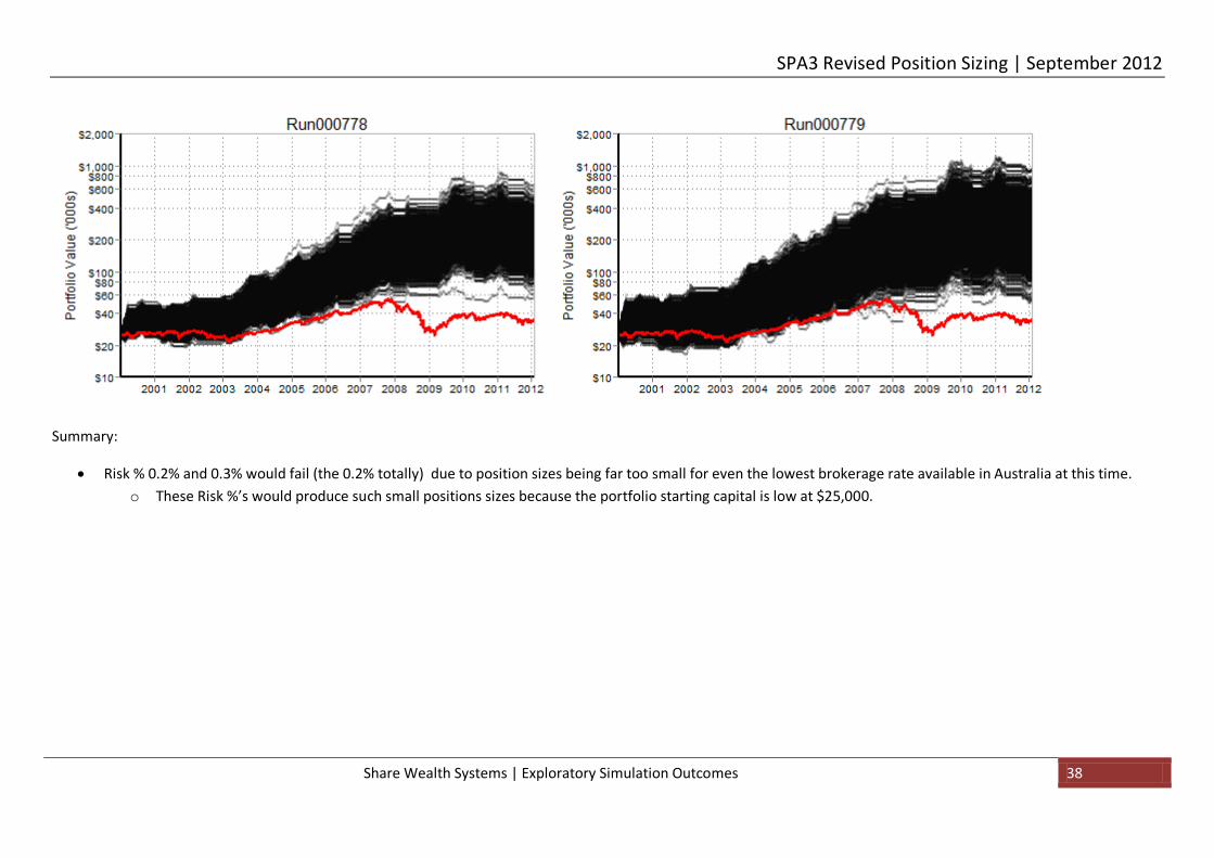
SPA3 Revised Position Sizing | September 2012
Share Wealth Systems | Exploratory Simulation Outcomes 38
Summary:
• Risk % 0.2% and 0.3% would fail (the 0.2% totally) due to position sizes being far too small for even the lowest brokerage rate available in Australia at this time. o These Risk %’s would produce such small positions sizes because the portfolio starting capital is low at $25,000.

SPA3 Revised Position Sizing | September 2012
Share Wealth Systems | Exploratory Simulation Outcomes 39
0
500
1000
1500
2000
2500
0.2 0.3 0.4 0.5 0.6 0.8 1.0 1.5 2.0 3.0
Risk %
Portfolio Performance Index
200101-201201, XASX SIROC 2108 25k Liq00 B9.90,0.1 (Risks)
0.5
0.6
0.7
0.8
0.9
1.0
1.1
1.2
0.2 0.3 0.4 0.5 0.6 0.8 1.0 1.5 2.0 3.0
Risk %
Downside Deviation Factor
200101-201201, XASX SIROC 2108 25k Liq00 B9.90,0.1 (Risks)
1
1.0001
1.0002
1.0003
1.0004
1.0005
1.0006
1.0007
1.0008
1.0009
1.001
0.2 0.3 0.4 0.5 0.6 0.8 1.0 1.5 2.0 3.0
Risk %
Daily Geometric Mean
200101-201201, XASX SIROC 2108 25k Liq00 B9.90,0.1 (Risks)
0
10
20
30
40
50
60
0.2 0.3 0.4 0.5 0.6 0.8 1.0 1.5 2.0 3.0
Risk %
Maximum Drawdown (%)
200101-201201, XASX SIROC 2108 25k Liq00 B9.90,0.1 (Risks)

SPA3 Revised Position Sizing | September 2012
Share Wealth Systems | Exploratory Simulation Outcomes 40
20
25
30
35
40
45
50
55
60
0.2 0.3 0.4 0.5 0.6 0.8 1.0 1.5 2.0 3.0
Risk %
Unallocated Equity Deviation (%)
200101-201201, XASX SIROC 2108 25k Liq00 B9.90,0.1 (Risks)
0
500
1,000
1,500
2,000
2,500
3,000
3,500
4,000
0.2 0.3 0.4 0.5 0.6 0.8 1.0 1.5 2.0 3.0
Risk %
Number of Transactions
200101-201201, XASX SIROC 2108 25k Liq00 B9.90,0.1 (Risks)
0.4
0.6
0.8
1.0
1.2
1.4
1.6
1.8
2.0
0.2 0.3 0.4 0.5 0.6 0.8 1.0 1.5 2.0 3.0
Risk %
Profit Ratio
200101-201201, XASX SIROC 2108 25k Liq00 B9.90,0.1 (Risks)
30
35
40
45
50
55
0.2 0.3 0.4 0.5 0.6 0.8 1.0 1.5 2.0 3.0
Risk %
Win Rate (%)
200101-201201, XASX SIROC 2108 25k Liq00 B9.90,0.1 (Risks)

SPA3 Revised Position Sizing | September 2012
Share Wealth Systems | Exploratory Simulation Outcomes 41
11.2.2 25k Charts: SIROC 2108, x5 Liquidity Check, $9.90 or 0.1% Brokerage
1. Run 780 0.2% Portfolio Risk %. 2. Run 781 0.3% 3. Run 782 0.4% 4. Run 783 0.5%. 5. Run 784 0.6%. 6. Run 785 0.8%. 7. Run 786 1%. 8. Run 787 1.5%. 9. Run 788 2%. 10. Run 789 3%.
Ensure that you read the detailed analysis provided at the end of section 11.2.3 on page 47 for the portfolio scenario of starting with a $25,000 portfolio with the SIROC 21 8 parameters.
The simulations run with SIROC 13 5 5 included scenarios with $25,000 starting capital with brokerage at $27.50 or 0.165%, and $19.95 or 0.1%. Ensure that you explore the outcomes of these simulations with the relatively high brokerage rate for a small starting portfolio. There are in section 11.3.2 on page 106.

SPA3 Revised Position Sizing | September 2012
Share Wealth Systems | Exploratory Simulation Outcomes 42
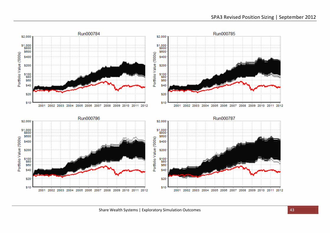
SPA3 Revised Position Sizing | September 2012
Share Wealth Systems | Exploratory Simulation Outcomes 43

SPA3 Revised Position Sizing | September 2012
Share Wealth Systems | Exploratory Simulation Outcomes 44
Summary:
• Risk % 0.2% and 0.3% would fail (the 0.2% totally) due to position sizes being far too small for even the lowest brokerage rate available in Australia at this time. o These Risk %’s would produce such small positions sizes because the portfolio starting capital is low at $25,000.
• Using the equity curve outcomes above and the box plots below: o Risk % of 1.5% should not be exceeded. o A Risk % under 0.5% should not be used.

SPA3 Revised Position Sizing | September 2012
Share Wealth Systems | Exploratory Simulation Outcomes 45
0
500
1000
1500
2000
2500
0.2 0.3 0.4 0.5 0.6 0.8 1.0 1.5 2.0 3.0
Risk %
Portfolio Performance Index
200101-201201, XASX SIROC 2108 25k Liq05 B9.90,0.1 (Risks)
0.5
0.6
0.7
0.8
0.9
1.0
1.1
1.2
0.2 0.3 0.4 0.5 0.6 0.8 1.0 1.5 2.0 3.0
Risk %
Downside Deviation Factor
200101-201201, XASX SIROC 2108 25k Liq05 B9.90,0.1 (Risks)
1
1.0001
1.0002
1.0003
1.0004
1.0005
1.0006
1.0007
1.0008
1.0009
1.001
0.2 0.3 0.4 0.5 0.6 0.8 1.0 1.5 2.0 3.0
Risk %
Daily Geometric Mean
200101-201201, XASX SIROC 2108 25k Liq05 B9.90,0.1 (Risks)
0
10
20
30
40
50
60
0.2 0.3 0.4 0.5 0.6 0.8 1.0 1.5 2.0 3.0
Risk %
Maximum Drawdown (%)
200101-201201, XASX SIROC 2108 25k Liq05 B9.90,0.1 (Risks)

SPA3 Revised Position Sizing | September 2012
Share Wealth Systems | Exploratory Simulation Outcomes 46
20
25
30
35
40
45
50
55
60
0.2 0.3 0.4 0.5 0.6 0.8 1.0 1.5 2.0 3.0
Risk %
Unallocated Equity Deviation (%)
200101-201201, XASX SIROC 2108 25k Liq05 B9.90,0.1 (Risks)
0
500
1,000
1,500
2,000
2,500
3,000
3,500
4,000
0.2 0.3 0.4 0.5 0.6 0.8 1.0 1.5 2.0 3.0
Risk %
Number of Transactions
200101-201201, XASX SIROC 2108 25k Liq05 B9.90,0.1 (Risks)
0.4
0.6
0.8
1.0
1.2
1.4
1.6
1.8
2.0
0.2 0.3 0.4 0.5 0.6 0.8 1.0 1.5 2.0 3.0
Risk %
Profit Ratio
200101-201201, XASX SIROC 2108 25k Liq05 B9.90,0.1 (Risks)
30
35
40
45
50
55
0.2 0.3 0.4 0.5 0.6 0.8 1.0 1.5 2.0 3.0
Risk %
Win Rate (%)
200101-201201, XASX SIROC 2108 25k Liq05 B9.90,0.1 (Risks)

SPA3 Revised Position Sizing | September 2012
Share Wealth Systems | Exploratory Simulation Outcomes 47
11.2.3 25k Charts: SIROC 2108, x10 Liquidity Check, $9.90 or 0.1% Brokerage
1. Run 790 0.2% Portfolio Risk %. 2. Run 791 0.3% 3. Run 792 0.4% 4. Run 793 0.5%. 5. Run 794 0.6%. 6. Run 795 0.8%. 7. Run 796 1%. 8. Run 797 1.5%. 9. Run 798 2%. 10. Run 799 3%.
The simulations run with SIROC 13 5 5 included scenarios with $25,000 starting capital with brokerage at $27.50 or 0.165%, and $19.95 or 0.1%. Ensure that you explore the outcomes of these simulations with the relatively high brokerage rate for a small starting portfolio. There are in section 11.3.2 on page 106.

SPA3 Revised Position Sizing | September 2012
Share Wealth Systems | Exploratory Simulation Outcomes 48

SPA3 Revised Position Sizing | September 2012
Share Wealth Systems | Exploratory Simulation Outcomes 49

SPA3 Revised Position Sizing | September 2012
Share Wealth Systems | Exploratory Simulation Outcomes 50
Summary:
• Risk % 0.2% and 0.3% would fail (the 0.2% totally) due to position sizes being far too small for even the lowest brokerage rate available in Australia at this time. o These Risk %’s would produce such small positions sizes because the portfolio starting capital is low at $25,000.
• Using the equity curve outcomes above and the box plots below: o Risk % of 1.5% should not be exceeded. A Risk % of 2% shows a falling Daily Geometric Mean box plot which means that the odds are stacked against being
more profitable than using a Risk % of 1.5%, 1.0% or even 0.8%. Also, Maximum Drawdown starts getting deeper with a 2% Risk %. o Maybe a maximum Risk % between 1.0% and 1.5% could be considered at around 1.2%. The reasons for this consideration are the falling PPI and rising
Downside Deviation Factor. o A Risk % under 0.5% should not be used.

SPA3 Revised Position Sizing | September 2012
Share Wealth Systems | Exploratory Simulation Outcomes 51
0
500
1000
1500
2000
2500
0.2 0.3 0.4 0.5 0.6 0.8 1.0 1.5 2.0 3.0
Risk %
Portfolio Performance Index
200101-201201, XASX SIROC 2108 25k Liq10 B9.90,0.1 (Risks)
0.5
0.6
0.7
0.8
0.9
1.0
1.1
1.2
0.2 0.3 0.4 0.5 0.6 0.8 1.0 1.5 2.0 3.0
Risk %
Downside Deviation Factor
200101-201201, XASX SIROC 2108 25k Liq10 B9.90,0.1 (Risks)
1
1.0001
1.0002
1.0003
1.0004
1.0005
1.0006
1.0007
1.0008
1.0009
1.001
0.2 0.3 0.4 0.5 0.6 0.8 1.0 1.5 2.0 3.0
Risk %
Daily Geometric Mean
200101-201201, XASX SIROC 2108 25k Liq10 B9.90,0.1 (Risks)
0
10
20
30
40
50
60
0.2 0.3 0.4 0.5 0.6 0.8 1.0 1.5 2.0 3.0
Risk %
Maximum Drawdown (%)
200101-201201, XASX SIROC 2108 25k Liq10 B9.90,0.1 (Risks)

SPA3 Revised Position Sizing | September 2012
Share Wealth Systems | Exploratory Simulation Outcomes 52
20
25
30
35
40
45
50
55
60
0.2 0.3 0.4 0.5 0.6 0.8 1.0 1.5 2.0 3.0
Risk %
Unallocated Equity Deviation (%)
200101-201201, XASX SIROC 2108 25k Liq10 B9.90,0.1 (Risks)
0
500
1,000
1,500
2,000
2,500
3,000
3,500
4,000
0.2 0.3 0.4 0.5 0.6 0.8 1.0 1.5 2.0 3.0
Risk %
Number of Transactions
200101-201201, XASX SIROC 2108 25k Liq10 B9.90,0.1 (Risks)
0.4
0.6
0.8
1.0
1.2
1.4
1.6
1.8
2.0
0.2 0.3 0.4 0.5 0.6 0.8 1.0 1.5 2.0 3.0
Risk %
Profit Ratio
200101-201201, XASX SIROC 2108 25k Liq10 B9.90,0.1 (Risks)
30
35
40
45
50
55
0.2 0.3 0.4 0.5 0.6 0.8 1.0 1.5 2.0 3.0
Risk %
Win Rate (%)
200101-201201, XASX SIROC 2108 25k Liq10 B9.90,0.1 (Risks)

SPA3 Revised Position Sizing | September 2012
Share Wealth Systems | Exploratory Simulation Outcomes 53
11.2.3.1 Individual Equity Curves & Underwater Equity Curves
Three individual equity curves have been plotted below using a Portfolio Risk % of 1.0% showing:
1. The portfolio equity curve compared to the All ORDS (XAO). 2. The number of open positions through the life of the portfolio. 3. The underwater equity curve which shows all the drawdown periods of that equity curve. 4. The underwater equity curve (black shadow) compared to the ALL ORDS underwater equity curve (red shadow).
The following three equity curves were selected:
1. The 50th percentile geometric mean which is the median return (499 had better & worse returns) at the end of the of simulated portfolio equity curves. 2. The 25th percentile maximum drawdown. This means that 25% of portfolios had a maximum drawdown LESS (i.e. better) than this particular equity curve. 3. The 95th percentile maximum drawdown. This means that 95% of portfolios had a maximum drawdown LESS (i.e. better) than this particular equity curve.

SPA3 Revised Position Sizing | September 2012
Share Wealth Systems | Exploratory Simulation Outcomes 54

SPA3 Revised Position Sizing | September 2012
Share Wealth Systems | Exploratory Simulation Outcomes 55

SPA3 Revised Position Sizing | September 2012
Share Wealth Systems | Exploratory Simulation Outcomes 56

SPA3 Revised Position Sizing | September 2012
Share Wealth Systems | Exploratory Simulation Outcomes 57
In each of the three scenarios above (and the 95th percentile geometric mean is also included in the last column for which there are no graphs above) the following additional information is provided to assist with understanding and positioning of the final outcomes in absolute terms rather than just relative terms:
The next table provides further statistical analysis of the different Portfolio Risk % selections from 0.3% to 3%. The top section of the table provides the 95th percentile of both the growth rate, i.e. the geometric mean, and the maximum drawdown. The middle section is the median, the 50th percentile, and bottom section the 25th percentile.
The 95th percentile is used for both geometric mean and maximum drawdown to determine the ‘worst case’ as it is unlikely that an active investor will have a deeper drawdown than the 95th percentile and it is unlikely that they will have a return that is less than the 95th percentile of the geometric mean, unless they break the rules a lot of the time due to poor trading psychology or disbelief in the methodology. However, it is still possible as many do just this.
The compounded annual return (CAGR) is divided by the maximum drawdown experienced throughout the life of the portfolio. This is an objective way of measuring the maximum risk taken to gain the long term reward that has been achieved. Using this ‘worst case’ scenario, i.e. the 95th percentile, of the maximum amount of portfolio value given back to the market, i.e. maximum portfolio drawdown, for the entire life of the portfolio and the 95th percentile of the annualised compounded return achieved by taking that risk, the active investor can conservatively determine the largest position size with which to trade.
In the table below this would be when the CAGR to Max DD ratio starts declining as the Portfolio Risk % increases. This is at 0.8%.
Looking at the 50th and 25th percentiles the position size could be increased by increasing the Portfolio Risk % to as large as 1.5%. However, this would be a far less conservative approach. As the Portfolio Risk % is increased the active investor’s portfolio return would be far more sensitive to trading errors which can ultimately be
Portfolio at the:Portfolio Risk % = 1.00% 25th Percentile 95th Percentile 50th Percentile 95th Percentile
XAO Max DD Max DD Gmean Gmean
Final Portfolio Value 34,434 240,993 130,470 171,524 115,963Daily Geometric Mean 1.000683 1.00048 1.000572 1.000445
Max Drawdown -54.60% -25.91% -36.66% -29.52% -34.91%Win Rate 46.38% 43.41% 45.25% 43.99%
Profit Ratio 1.5 1.32 1.39 1.32# of Trades 607 599 589 587
CAGR 2.73% 20.63% 14.65% 17.28% 13.54%Max DD Percentile 25 95 63 92
Geometric Mean Percentile 7 88 50 95CAGR / Max DD 0.05 0.7962 0.3996 0.5854 0.3879

SPA3 Revised Position Sizing | September 2012
Share Wealth Systems | Exploratory Simulation Outcomes 58
defined as not following the rules of the methodology due to many and varied reasons. However, the potential reward is on offer provided the trader believes that they can manage their portfolio such that they can result in reaching the median (50th percentile) or even the 25th percentile. This is where improving one’s trading skills can be of great benefit. With better skills more risk can be taken by increasing the positions, to a point, but beware of potentially deeper drawdowns.
Lastly, these ratios will differ from system to system and for different position sizes used for each system. Also, the market performance and the term over which the ratio is calculated will result in different ratio outcomes. Over this sample period compare the CAGR to Max DD ratio for the All Ordinaries Index at 0.05 to get an idea of the risk taken for reward gained compared to the overall market, i.e. to get an indication of the risk for reward that was on offer from the market, or a buy and hold portfolio.
These ratios are best shown in the graphs below that plot the CAGR to Max DD ratios for each Portfolio Risk % from 0.3% to 3%. The CAGR to Max DD Ratio is plotted on the vertical scale and the Portfolio Risk % along the horizontal scale. More conservative active investors should use the 95th Percentile graph to select their position size and not go larger than 0.1% whereas those that believe they will make few trading errors may wish to increase their Portfolio Risk % but not too much higher than 1.5%.
Portfolio Risk % XAO 0.3% 0.4% 0.5% 0.6% 0.8% 1.0% 1.5% 2.0% 3.0%
95th Percentile Geometric Mean 1.000152 1.000343 1.000385 1.000411 1.000439 1.000445 1.000424 1.000393 1.000329End Portfolio Value 34,434 43,329 77,410 91,243 99,911 111,797 115,963 113,201 111,359 103,216
Compunded Annual Growth 2.73% 4.66% 9.81% 11.31% 12.15% 13.20% 13.54% 13.31% 13.16% 12.45%95th Percentile Max Drawdown -54.60% -38.45% -34.59% -33.61% -33.61% -33.45% -36.66% -37.09% -40.20% -45.17%
CAGR/MaxDD 0.0500 0.1212 0.2836 0.3365 0.3615 0.3946 0.3693 0.3589 0.3274 0.2756
50th Percentile Geometric Mean 1.000218 1.000403 1.000475 1.000509 1.000547 1.000572 1.000584 1.000559 1.000489End Portfolio Value 34,434 53,363 95,128 120,842 134,608 154,339 171,524 189,723 179,808 160,735
Compunded Annual Growth 2.73% 6.48% 11.70% 13.93% 14.95% 16.26% 17.26% 18.26% 17.74% 16.65%50th Percentile Max Drawdown -54.60% -34.06% -29.42% -27.79% -27% -27.40% -28.10% -28.06% -30.70% -33.30%
CAGR/MaxDD 0.0500 0.1903 0.3977 0.5013 0.5537 0.5934 0.6142 0.6507 0.5779 0.5000
25th Percentile Geometric Mean 1.000245 1.000435 1.000509 1.00055 1.000592 1.000619 1.000641 1.000613 1.000562End Portfolio Value 34,434 57,937 105,189 133,828 153,506 177,690 198390 222,601 218,263 199,146
Compunded Annual Growth 2.73% 7.20% 12.63% 14.90% 16.21% 17.62% 18.70% 19.84% 19.64% 18.74%25th Percentile Max Drawdown -54.60% -32.27% -26.93% -25.78% -25.17% -25.26% -25.91% -25.90% -27.88% -30.30%
CAGR/MaxDD 0.0500 0.2231 0.4690 0.5780 0.6440 0.6975 0.7217 0.7660 0.7044 0.6185

SPA3 Revised Position Sizing | September 2012
Share Wealth Systems | Exploratory Simulation Outcomes 59

SPA3 Revised Position Sizing | September 2012
Share Wealth Systems | Exploratory Simulation Outcomes 60
It should be noted that using a CAGR over a long term period such as 12 years is far more robust that doing the same over a shorter period such as 1 – 5 years which would be more susceptible to not including multiple up and down markets. It is strongly advised that whatever period is used to determine the CAGR and Maximum Drawdown for equities portfolios, that at least two down markets of at least 20% are included and that at least one up market of greater than 50% is included in the research period. Otherwise the respective figures for these two measurements could be skewed too positively.
The detail is provided in these tables as much as for determining the best position size with which to trade as to also convince active investors, SPA3 and otherwise, NOT to trade with position sizes that are too large. Note how quickly the odds decline with the position size at 2% and 3% Risk % per trade. That is, taking more risk with larger positions sizes makes no sense as the corresponding return is not forthcoming. The major reason that the expected return does not eventuate is due to volatility drag. Volatility drag is explained in the Appendices to this White Paper.
On the other side of the spectrum with small position sizes, once too small a position size is used, the odds of gaining sound returns for the risk taken also falls away. But the reason on this side of the spectrum is totally different. Theoretically, provided there are sufficient positions to fill ones portfolio, returns should continue to improve relative to drawdown as position sizes decrease because portfolio volatility drag decreases. This would be so if no brokerage was due. Minimum brokerage rates cause portfolio performance to decrease as position sizes decrease to the point of portfolio meltdown when position sizes are too small relative to the portfolio capital and the average gains that the trading system produces.
This detailed analysis is repeated for a $100,000 portfolio scenario in section 11.2.6.1 on page 80.

SPA3 Revised Position Sizing | September 2012
Share Wealth Systems | Exploratory Simulation Outcomes 61
11.2.4 100k Charts: SIROC 2108, No Liquidity Check, $27.50 or 0.165% Brokerage
1. Run 740 0.2% Portfolio Risk %. 2. Run 741 0.3% 3. Run 742 0.4% 4. Run 743 0.5%. 5. Run 744 0.6%. 6. Run 745 0.8%. 7. Run 746 1%. 8. Run 747 1.5%. 9. Run 748 2%. 10. Run 749 3%.
This simulation has no liquidity check which means that any trade that met the SPA3 entry criteria could be entered regardless of how illiquid the trade. Whilst unrealistic, this simulation has been run and included in the White Paper to show a base case against which to compare simulations that do include liquidity checks.

SPA3 Revised Position Sizing | September 2012
Share Wealth Systems | Exploratory Simulation Outcomes 62

SPA3 Revised Position Sizing | September 2012
Share Wealth Systems | Exploratory Simulation Outcomes 63
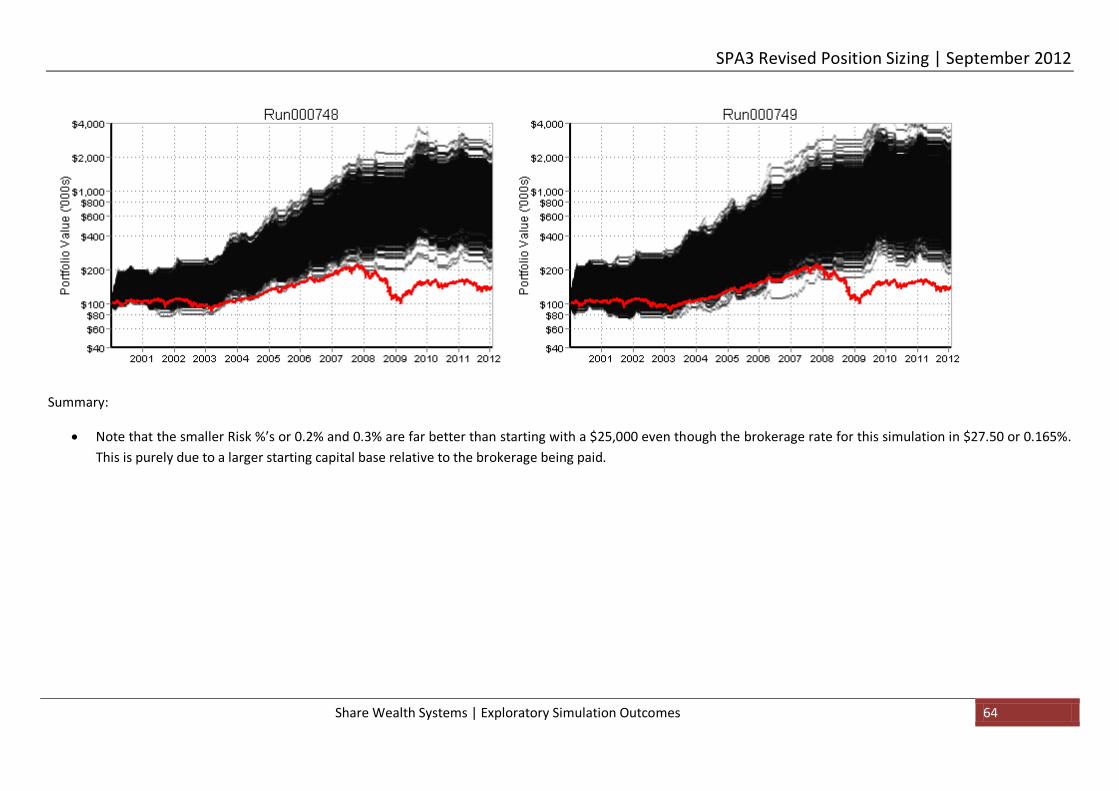
SPA3 Revised Position Sizing | September 2012
Share Wealth Systems | Exploratory Simulation Outcomes 64
Summary:
• Note that the smaller Risk %’s or 0.2% and 0.3% are far better than starting with a $25,000 even though the brokerage rate for this simulation in $27.50 or 0.165%. This is purely due to a larger starting capital base relative to the brokerage being paid.

SPA3 Revised Position Sizing | September 2012
Share Wealth Systems | Exploratory Simulation Outcomes 65
0
500
1000
1500
2000
2500
0.2 0.3 0.4 0.5 0.6 0.8 1.0 1.5 2.0 3.0
Risk %
Portfolio Performance Index
200101-201201, XASX SIROC 2108 100k Liq00 (Risks)
0.5
0.6
0.7
0.8
0.9
1.0
1.1
1.2
0.2 0.3 0.4 0.5 0.6 0.8 1.0 1.5 2.0 3.0
Risk %
Downside Deviation Factor
200101-201201, XASX SIROC 2108 100k Liq00 (Risks)
1
1.0001
1.0002
1.0003
1.0004
1.0005
1.0006
1.0007
1.0008
1.0009
1.001
0.2 0.3 0.4 0.5 0.6 0.8 1.0 1.5 2.0 3.0
Risk %
Daily Geometric Mean
200101-201201, XASX SIROC 2108 100k Liq00 (Risks)
0
10
20
30
40
50
60
0.2 0.3 0.4 0.5 0.6 0.8 1.0 1.5 2.0 3.0
Risk %
Maximum Drawdown (%)
200101-201201, XASX SIROC 2108 100k Liq00 (Risks)

SPA3 Revised Position Sizing | September 2012
Share Wealth Systems | Exploratory Simulation Outcomes 66
20
25
30
35
40
45
50
55
60
0.2 0.3 0.4 0.5 0.6 0.8 1.0 1.5 2.0 3.0
Risk %
Unallocated Equity Deviation (%)
200101-201201, XASX SIROC 2108 100k Liq00 (Risks)
0
500
1,000
1,500
2,000
2,500
3,000
3,500
4,000
0.2 0.3 0.4 0.5 0.6 0.8 1.0 1.5 2.0 3.0
Risk %
Number of Transactions
200101-201201, XASX SIROC 2108 100k Liq00 (Risks)
0.4
0.6
0.8
1.0
1.2
1.4
1.6
1.8
2.0
0.2 0.3 0.4 0.5 0.6 0.8 1.0 1.5 2.0 3.0
Risk %
Profit Ratio
200101-201201, XASX SIROC 2108 100k Liq00 (Risks)
30
35
40
45
50
55
0.2 0.3 0.4 0.5 0.6 0.8 1.0 1.5 2.0 3.0
Risk %
Win Rate (%)
200101-201201, XASX SIROC 2108 100k Liq00 (Risks)
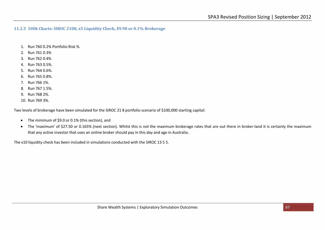
SPA3 Revised Position Sizing | September 2012
Share Wealth Systems | Exploratory Simulation Outcomes 67
11.2.5 100k Charts: SIROC 2108, x5 Liquidity Check, $9.90 or 0.1% Brokerage
1. Run 760 0.2% Portfolio Risk %. 2. Run 761 0.3% 3. Run 762 0.4% 4. Run 763 0.5%. 5. Run 764 0.6%. 6. Run 765 0.8%. 7. Run 766 1%. 8. Run 767 1.5%. 9. Run 768 2%. 10. Run 769 3%.
Two levels of brokerage have been simulated for the SIROC 21 8 portfolio scenario of $100,000 starting capital:
• The minimum of $9.0 or 0.1% (this section), and • The ‘maximum’ of $27.50 or 0.165% (next section). Whilst this is not the maximum brokerage rates that are out there in broker-land it is certainly the maximum
that any active investor that uses an online broker should pay in this day and age in Australia.
The x10 liquidity check has been included in simulations conducted with the SIROC 13 5 5.

SPA3 Revised Position Sizing | September 2012
Share Wealth Systems | Exploratory Simulation Outcomes 68

SPA3 Revised Position Sizing | September 2012
Share Wealth Systems | Exploratory Simulation Outcomes 69

SPA3 Revised Position Sizing | September 2012
Share Wealth Systems | Exploratory Simulation Outcomes 70
Summary:
• With a larger capital base, the 0.2% and 0.3% Risk % simulated equity curves look fantastic with very small variation of outcomes. However, a glance at the box plots below for PPI and Geometric Mean reveal that the active investor would taking too much risk and doing far too many round trip completed trades at 15.9 per month (4600/2/12.08/12 – transactions/2/years/months) for the relative rewards that would flow.
• Using the equity curve outcomes above and the box plots below: o Risk % of 1.0% should not be exceeded. A Risk % of 1.5% shows a falling Daily Geometric Mean box plot which means that the odds are stacked against
being more profitable than using a Risk % of 1.0%, down to 0.3%. Also, Maximum Drawdown starts getting deeper with a 1.5% Risk %. o A Risk % under 0.3% should not be used.
• Note the number of simultaneously Open Positions for 0.2% - 0.5% Risk % for the life of a portfolio that starts with $100,000, 3 pages hence.
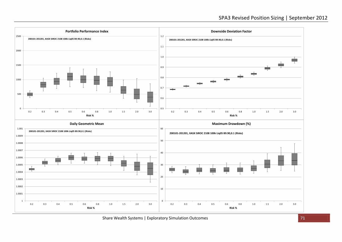
SPA3 Revised Position Sizing | September 2012
Share Wealth Systems | Exploratory Simulation Outcomes 71
0
500
1000
1500
2000
2500
0.2 0.3 0.4 0.5 0.6 0.8 1.0 1.5 2.0 3.0
Risk %
Portfolio Performance Index
200101-201201, XASX SIROC 2108 100k Liq05 B9.90,0.1 (Risks)
0.5
0.6
0.7
0.8
0.9
1.0
1.1
1.2
0.2 0.3 0.4 0.5 0.6 0.8 1.0 1.5 2.0 3.0
Risk %
Downside Deviation Factor
200101-201201, XASX SIROC 2108 100k Liq05 B9.90,0.1 (Risks)
1
1.0001
1.0002
1.0003
1.0004
1.0005
1.0006
1.0007
1.0008
1.0009
1.001
0.2 0.3 0.4 0.5 0.6 0.8 1.0 1.5 2.0 3.0
Risk %
Daily Geometric Mean
200101-201201, XASX SIROC 2108 100k Liq05 B9.90,0.1 (Risks)
0
10
20
30
40
50
60
0.2 0.3 0.4 0.5 0.6 0.8 1.0 1.5 2.0 3.0
Risk %
Maximum Drawdown (%)
200101-201201, XASX SIROC 2108 100k Liq05 B9.90,0.1 (Risks)

SPA3 Revised Position Sizing | September 2012
Share Wealth Systems | Exploratory Simulation Outcomes 72
20
25
30
35
40
45
50
55
60
0.2 0.3 0.4 0.5 0.6 0.8 1.0 1.5 2.0 3.0
Risk %
Unallocated Equity Deviation (%)
200101-201201, XASX SIROC 2108 100k Liq05 B9.90,0.1 (Risks)
0
500
1,000
1,500
2,000
2,500
3,000
3,500
4,000
0.2 0.3 0.4 0.5 0.6 0.8 1.0 1.5 2.0 3.0
Risk %
Number of Transactions
200101-201201, XASX SIROC 2108 100k Liq05 B9.90,0.1 (Risks)
0.4
0.6
0.8
1.0
1.2
1.4
1.6
1.8
2.0
0.2 0.3 0.4 0.5 0.6 0.8 1.0 1.5 2.0 3.0
Risk %
Profit Ratio
200101-201201, XASX SIROC 2108 100k Liq05 B9.90,0.1 (Risks)
30
35
40
45
50
55
0.2 0.3 0.4 0.5 0.6 0.8 1.0 1.5 2.0 3.0
Risk %
Win Rate (%)
200101-201201, XASX SIROC 2108 100k Liq05 B9.90,0.1 (Risks)

SPA3 Revised Position Sizing | September 2012
Share Wealth Systems | Exploratory Simulation Outcomes 73
SPA3 Revised Position Sizing | September 2012
Share Wealth Systems | Exploratory Simulation Outcomes 74
11.2.6 100k Charts: SIROC 2108, x5 Liquidity Check, $27.50 or 0.165% Brokerage
1. Run 750 0.2% Portfolio Risk %. 2. Run 751 0.3% 3. Run 752 0.4% 4. Run 753 0.5%. 5. Run 754 0.6%. 6. Run 755 0.8%. 7. Run 756 1%. 8. Run 757 1.5%. 9. Run 758 2%. 10. Run 759 3%.
$27.50 or 0.165%, whichever is the greatest, has been used as an ‘upper limit’ type brokerage for online trading in Australia meaning that most SPA3 active investors should be able to get a better brokerage rate than this. The lower the minimum brokerage rate the better, i.e. the $27.50 minimum before the scaling percentage of 0.165% kicks in, as most buy and sell transactions will be executed at this rate.
From all the simulations provided in this White Paper it should be obvious that if a Portfolio Risk % is used that is sound for this relatively high level of brokerage then it can only be better if a lower brokerage rate can be negotiated with a broker. In such instances, the Portfolio Risk % might be able to be increased slightly by .1% or even .2%. The SPA3 active investor will need to use their analysis of other simulation scenarios in this White Paper and a dose of common sense as to how much more risk they might take given their set of execution circumstances.
The x10 liquidity check has been included in simulations conducted with the SIROC 13 5 5.
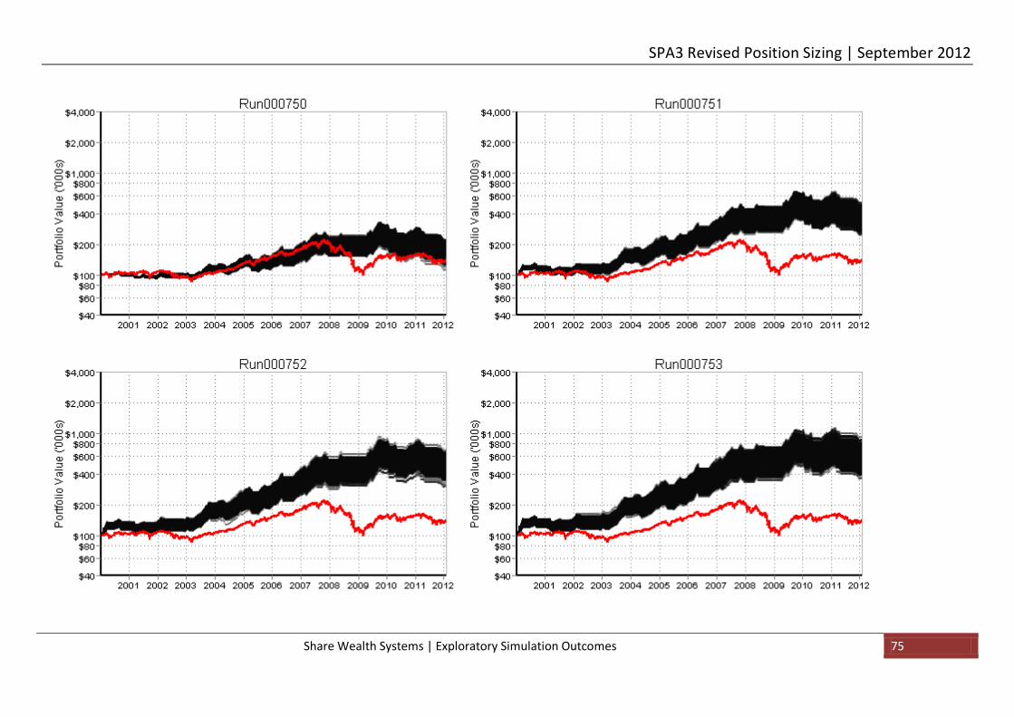
SPA3 Revised Position Sizing | September 2012
Share Wealth Systems | Exploratory Simulation Outcomes 75

SPA3 Revised Position Sizing | September 2012
Share Wealth Systems | Exploratory Simulation Outcomes 76

SPA3 Revised Position Sizing | September 2012
Share Wealth Systems | Exploratory Simulation Outcomes 77
Summary:
• With the higher brokerage rate the 0.2% Risk % becomes unviable. • Using the equity curve outcomes above and the box plots below:
o Risk % of 1.0% should not be exceeded. A Risk % of 1.5% shows a falling Daily Geometric Mean box plot which means that the odds are stacked against being more profitable than using a Risk % of 1.0%, down to 0.5%. Also, Maximum Drawdown starts getting deeper with a 1.5% Risk %.
o A Risk % under 0.4% should not be used. o Whilst 0.7% and 0.9% haven’t been simulated they could obviously also be used by as the Risk %. o With the range of Risk % between 0.5% and 1.0% all being very viable the major point of discernment might be the number of transactions.

SPA3 Revised Position Sizing | September 2012
Share Wealth Systems | Exploratory Simulation Outcomes 78
0
500
1000
1500
2000
2500
0.2 0.3 0.4 0.5 0.6 0.8 1.0 1.5 2.0 3.0
Risk %
Portfolio Performance Index
200101-201201, XASX SIROC 2108 100k Liq05 (Risks)
0.5
0.6
0.7
0.8
0.9
1.0
1.1
1.2
0.2 0.3 0.4 0.5 0.6 0.8 1.0 1.5 2.0 3.0
Risk %
Downside Deviation Factor
200101-201201, XASX SIROC 2108 100k Liq05 (Risks)
1
1.0001
1.0002
1.0003
1.0004
1.0005
1.0006
1.0007
1.0008
1.0009
1.001
0.2 0.3 0.4 0.5 0.6 0.8 1.0 1.5 2.0 3.0
Risk %
Daily Geometric Mean
200101-201201, XASX SIROC 2108 100k Liq05 (Risks)
0
10
20
30
40
50
60
0.2 0.3 0.4 0.5 0.6 0.8 1.0 1.5 2.0 3.0
Risk %
Maximum Drawdown (%)
200101-201201, XASX SIROC 2108 100k Liq05 (Risks)

SPA3 Revised Position Sizing | September 2012
Share Wealth Systems | Exploratory Simulation Outcomes 79
20
25
30
35
40
45
50
55
60
0.2 0.3 0.4 0.5 0.6 0.8 1.0 1.5 2.0 3.0
Risk %
Unallocated Equity Deviation (%)
200101-201201, XASX SIROC 2108 100k Liq05 (Risks)
0
500
1,000
1,500
2,000
2,500
3,000
3,500
4,000
0.2 0.3 0.4 0.5 0.6 0.8 1.0 1.5 2.0 3.0
Risk %
Number of Transactions
200101-201201, XASX SIROC 2108 100k Liq05 (Risks)
0.4
0.6
0.8
1.0
1.2
1.4
1.6
1.8
2.0
0.2 0.3 0.4 0.5 0.6 0.8 1.0 1.5 2.0 3.0
Risk %
Profit Ratio
200101-201201, XASX SIROC 2108 100k Liq05 (Risks)
30
35
40
45
50
55
0.2 0.3 0.4 0.5 0.6 0.8 1.0 1.5 2.0 3.0
Risk %
Win Rate (%)
200101-201201, XASX SIROC 2108 100k Liq05 (Risks)

SPA3 Revised Position Sizing | September 2012
Share Wealth Systems | Exploratory Simulation Outcomes 80
11.2.6.1 Individual Equity Curves & Underwater Equity Curves
Three individual equity curves have been plotted using a Portfolio Risk % of 0.8% from Run 755, showing:
1. The mark-to-market equity curve in arithmetic and log mode. The red plot is the All Ordinaries Index. 2. The % drawdown underwater equity curve vertical axis is scaled according to the maximum drawdown reached in the life of the portfolio. 3. The underwater curve for the portfolio (black shadow) compared to the underwater curve for the All Ordinaries Index (red shadow). 4. The open positions through the life of the portfolio. The periods where they are no open positions are when the portfolio was 100% in cash during High Market Risk
periods, according to Risk Profile 1.
The following three equity curves were selected:
1. The 50th percentile geometric mean which is the median return (499 had better & worse returns) at the end of the of simulated portfolio equity curves. 2. The 25th percentile maximum drawdown. This means that 25% of portfolios had a maximum drawdown LESS (i.e. better) than this particular equity curve. 3. The 95th percentile maximum drawdown. This means that 95% of portfolios had a maximum drawdown LESS (i.e. better) than this particular equity curve.
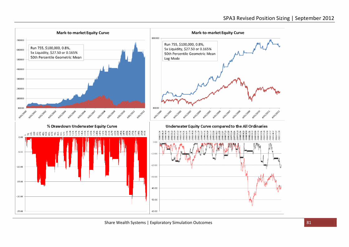
SPA3 Revised Position Sizing | September 2012
Share Wealth Systems | Exploratory Simulation Outcomes 81
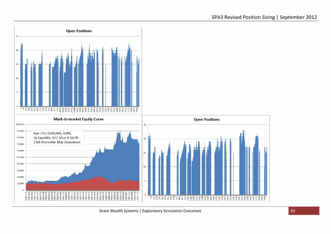
SPA3 Revised Position Sizing | September 2012
Share Wealth Systems | Exploratory Simulation Outcomes 82

SPA3 Revised Position Sizing | September 2012
Share Wealth Systems | Exploratory Simulation Outcomes 83

SPA3 Revised Position Sizing | September 2012
Share Wealth Systems | Exploratory Simulation Outcomes 84
In each of the three scenarios above (and the 95th percentile geometric mean is also included in the last column for which there are no graphs above) the following additional information is provided to assist with understanding and positioning of the final outcomes:

SPA3 Revised Position Sizing | September 2012
Share Wealth Systems | Exploratory Simulation Outcomes 85
In the next table that follows, the CAGR to Maximum Drawdown Ratios are provided in the same way that they were provided for the $25,000 portfolios with the SIROC 21 8 parameter settings in section 11.2.3 on page 53. You may wish to refer back there for further background on the CAGR to Maximum Drawdown Ratio.
The detail provided in these tables is as much as for determining the best position size with which to trade as it is to also convince active investors, SPA3 and otherwise, NOT to trade with position sizes that are too large. Note how quickly the odds decline with the position size at 2% and 3% Risk % per Trade. That is, taking more risk with larger positions sizes makes no sense as the corresponding return is not forthcoming. The major reason that the expected return does not eventuate is due to volatility drag. Volatility drag is explained in the Appendices to this White Paper.
On the other side of the spectrum with small position sizes, once too small a position size is used, the odds of gaining sound returns for the risk taken also falls away. But the reason on this side of the spectrum is totally different. Theoretically, provided there are sufficient positions to fill ones portfolio, returns should continue to improve relative to drawdown as position sizes decrease because portfolio volatility drag decreases. This would be so if no brokerage was due. Minimum brokerage rates cause portfolio performance to decrease as position sizes decrease to the point of portfolio meltdown when position sizes are too small relative to the portfolio capital and the average gains that the trading system produces.
Portfolio at the:Portfolio Risk % = 0.8% 25th Percentile 95th Percentile 50th Percentile 95th Percentile
XAO Max DD Max DD Gmean Gmean
Final Portfolio Value 138,462 719,335 491,539 621,178 451,120Daily Geometric Mean 1.000592 1.000474 1.000543 1.000443
Max Drawdown -54.60% -24.76% -34.32% -22.54% -34.86%Win Rate 45.76% 45.82% 45.82% 43.99%
Profit Ratio 1.46 1.34 1.45 1.31# of Trades 708 700 735 732
CAGR 2.73% 17.74% 14.09% 16.32% 13.28%Max DD Percentile 25 95 5 96
Geometric Mean Percentile 18 87 50 95CAGR / Max DD 0.0500 0.7165 0.4105 0.7240 0.3810

SPA3 Revised Position Sizing | September 2012
Share Wealth Systems | Exploratory Simulation Outcomes 86
This ratio is best shown in the graphs below that plot the CAGR to Max DD ratios for each Portfolio Risk % from 0.2% to 3%. The CAGR to Max DD Ratio is plotted on the vertical scale and the Portfolio Risk % along the horizontal scale. More conservative active investors should use the 95th Percentile graph to select their position size and not go larger than 0.7% or 0.8% Risk % whereas those that believe they will make few trading errors may wish to increase their Portfolio Risk % but not too much higher than 1%.
Portfolio Risk % XAO 0.2% 0.3% 0.4% 0.5% 0.6% 0.8% 1.0% 1.5% 2.0% 3.0%
95th Percentile Geometric Mean 1.000089 1.000326 1.000413 1.000455 1.000463 1.000443 1.000439 1.000404 1.000341 1.00024End Portfolio Value 138,462 141,241 297,551 393,175 451,349 466,862 451,120 454,733 432,729 367,461 293,150
Compunded Annual Growth 2.73% 2.90% 9.44% 12.00% 13.28% 13.60% 13.28% 13.35% 12.89% 11.37% 9.31%95th Percentile Max Drawdown -54.60% -39.11% -32.67% -31.80% -32.34% -33.45% -34.32% -33.93% -40.23% -45.03% -48.69%
CAGR/MaxDD 0.0500 0.0741 0.2890 0.3774 0.4106 0.4066 0.3869 0.3935 0.3204 0.2525 0.1912
50th Percentile Geometric Mean 1.000146 1.00039 1.000487 1.000527 1.000544 1.000543 1.000548 1.0005 1.000454 1.000436End Portfolio Value 138,462 167,943 361,307 491,060 566,073 599,802 621,178 637,311 572,394 526,942 520,015
Compunded Annual Growth 2.73% 4.38% 11.22% 14.08% 15.43% 15.98% 16.32% 16.57% 15.53% 14.75% 14.62%50th Percentile Max Drawdown -54.60% -36.29% -28.71% -26.61% -26.62% -27.03% -26.81% -27.61% -30.90% -33.68% -34.94%
CAGR/MaxDD 0.0500 0.1207 0.3908 0.5291 0.5796 0.5912 0.6087 0.6001 0.5026 0.4379 0.4184
25th Percentile Geometric Mean 1.000171 1.000416 1.000508 1.000568 1.000569 1.000582 1.000589 1.00054 1.00052 1.000576End Portfolio Value 138,462 181,875 392,022 528,227 641,614 653,443 684,466 721,277 642,941 649,342 677,137
Compunded Annual Growth 2.73% 5.08% 11.97% 14.77% 16.63% 16.81% 17.26% 17.77% 16.65% 16.75% 17.15%25th Percentile Max Drawdown -54.60% -34.99% -26.66% -25.03% -25.01% -25.19% -24.76% -25.29% -27.71% -30.03% -30.33%
CAGR/MaxDD 0.0500 0.1452 0.4490 0.5901 0.6649 0.6673 0.6971 0.7026 0.6009 0.5578 0.5654

SPA3 Revised Position Sizing | September 2012
Share Wealth Systems | Exploratory Simulation Outcomes 87

SPA3 Revised Position Sizing | September 2012
Share Wealth Systems | Exploratory Simulation Outcomes 88
Before leaving this portfolio scenario we include a scenario of how a simulation performed from the period starting 1 October 2007 leading into primary bear market of 2008. When the portfolio simulations above (from Runs 750 – 759) that started with $100,000 arrived at this point, they were well above $400,000 to $500,000. So we have chosen a portfolio scenario that started with $25,000 and reached $90,000 by the top of the 2008 bear market.
Because the main risk management rule that is used is Risk Profile 1, portfolios are restarted at the beginning of every Low Market Risk period. The scenario below starts at the beginning or the last Low Risk market just prior to the 2008 bear market, 1 October 2007. The portfolio equity that we chose was the one that ended at the 95th percentile by growth (i.e. by geometric mean, 5% performed worse and 95% performed better) as at 31 January 2012. Note this is over the entire research period from Jan 2000 to Jan 2012. This does not mean that it would have been at the 95th percentile by growth over the 1 October 2007 to January 2012 period. Finding this particular portfolio would be very a tedious manual process of looking through 1000 portfolios manually. At some stage we will run portfolio simulations starting at this date but we couldn’t complete this task for this paper.
Looking that $25,000 portfolio scenario’s from the end of 2007 will provide SPA3 active investors with a good idea how $100,000 portfolios would have fared since then to the beginning of 2012.

SPA3 Revised Position Sizing | September 2012
Share Wealth Systems | Exploratory Simulation Outcomes 89

SPA3 Revised Position Sizing | September 2012
Share Wealth Systems | Exploratory Simulation Outcomes 90
11.2.7 400k Charts: SIROC 2108, x5 Liquidity Check, $27.50 or 0.165% Brokerage
1. Run 810 0.2% Portfolio Risk %. 2. Run 811 0.3% 3. Run 812 0.4% 4. Run 813 0.5%. 5. Run 814 0.6%. 6. Run 815 0.8%. 7. Run 816 1%. 8. Run 817 1.5%. 9. Run 818 2%. 10. Run 819 3%.
We have only run one $400,000 simulation on the highest brokerage rate as any lower brokerage rate would only have a positive effect. At this size of portfolio and higher $27.50 minimum brokerage does not have the same level of adverse effect as $100,000 and $25,000 starting capitals.

SPA3 Revised Position Sizing | September 2012
Share Wealth Systems | Exploratory Simulation Outcomes 91

SPA3 Revised Position Sizing | September 2012
Share Wealth Systems | Exploratory Simulation Outcomes 92

SPA3 Revised Position Sizing | September 2012
Share Wealth Systems | Exploratory Simulation Outcomes 93
Summary:
• Whilst 0.2% Risk % becomes viable from a brokerage and return viewpoint but the number of simultaneously open positions will probably be too active for most. • Using the equity curve outcomes above and the box plots below:
o Risk % of 0.6% should not be exceeded. A Risk % of 0.8% shows a falling Daily Geometric Mean box plot which means that the odds are stacked against being more profitable than using a Risk % of 0.6%, down to 0.2%. Also, Maximum Drawdown starts getting deeper with a 0.8% Risk %.
o A Risk % under 0.2% should not be used. o With the range of Risk % between 0.2% and 0.6% all being very viable the major point of discernment might be the number of transactions.

SPA3 Revised Position Sizing | September 2012
Share Wealth Systems | Exploratory Simulation Outcomes 94
0
500
1000
1500
2000
2500
0.2 0.3 0.4 0.5 0.6 0.8 1.0 1.5 2.0 3.0
Risk %
Portfolio Performance Index
200101-201201, XASX SIROC 2108 400k Liq05 (Risks)
0.5
0.6
0.7
0.8
0.9
1.0
1.1
1.2
0.2 0.3 0.4 0.5 0.6 0.8 1.0 1.5 2.0 3.0
Risk %
Downside Deviation Factor
200101-201201, XASX SIROC 2108 400k Liq05 (Risks)
1
1.0001
1.0002
1.0003
1.0004
1.0005
1.0006
1.0007
1.0008
1.0009
1.001
0.2 0.3 0.4 0.5 0.6 0.8 1.0 1.5 2.0 3.0
Risk %
Daily Geometric Mean
200101-201201, XASX SIROC 2108 400k Liq05 (Risks)
0
10
20
30
40
50
60
0.2 0.3 0.4 0.5 0.6 0.8 1.0 1.5 2.0 3.0
Risk %
Maximum Drawdown (%)
200101-201201, XASX SIROC 2108 400k Liq05 (Risks)

SPA3 Revised Position Sizing | September 2012
Share Wealth Systems | Exploratory Simulation Outcomes 95
20
25
30
35
40
45
50
55
60
0.2 0.3 0.4 0.5 0.6 0.8 1.0 1.5 2.0 3.0
Risk %
Unallocated Equity Deviation (%)
200101-201201, XASX SIROC 2108 400k Liq05 (Risks)
0
500
1,000
1,500
2,000
2,500
3,000
3,500
4,000
0.2 0.3 0.4 0.5 0.6 0.8 1.0 1.5 2.0 3.0
Risk %
Number of Transactions
200101-201201, XASX SIROC 2108 400k Liq05 (Risks)
0.4
0.6
0.8
1.0
1.2
1.4
1.6
1.8
2.0
0.2 0.3 0.4 0.5 0.6 0.8 1.0 1.5 2.0 3.0
Risk %
Profit Ratio
200101-201201, XASX SIROC 2108 400k Liq05 (Risks)
30
35
40
45
50
55
0.2 0.3 0.4 0.5 0.6 0.8 1.0 1.5 2.0 3.0
Risk %
Win Rate (%)
200101-201201, XASX SIROC 2108 400k Liq05 (Risks)

SPA3 Revised Position Sizing | September 2012
Share Wealth Systems | Exploratory Simulation Outcomes 96
11.2.7.1 Individual Equity Curves & Underwater Equity Curves
The Open Positions charts above show the number of simultaneous open positions for a 0.2%, 0.3% and 0.5% Portfolio Risk %, as per Runs 810, 811 and 813. 0.2% and 0.3% will be a comparatively high number of positions to manage for most private active investors. 0.4%, as shown below, may still be a little on the high side but the risk to reward at this Risk % may make it worthwhile. 0.5% and 0.6% should be just fine.
Two individual equity curves have been plotted below using a Portfolio Risk % of 0.4% showing:
1. The portfolio equity curve compared to the All ORDS (XAO). 2. The number of open positions through the life of the portfolio. 3. The underwater equity curve which shows all the drawdown periods of that equity curve. 4. The underwater equity curve (black shadow) compared to the ALL ORDS underwater equity curve (red shadow).
The following two equity curves from the sample of the 1000 simulated equity curves were selected:
1. The 50th percentile geometric mean which is the median return (499 had better & worse returns) at the end of the of simulated portfolio equity curves. 2. The 95th percentile maximum drawdown. This means that 95% of portfolios had a maximum drawdown LESS (i.e. better or shallower) than this particular equity
curve.

SPA3 Revised Position Sizing | September 2012
Share Wealth Systems | Exploratory Simulation Outcomes 97

SPA3 Revised Position Sizing | September 2012
Share Wealth Systems | Exploratory Simulation Outcomes 98
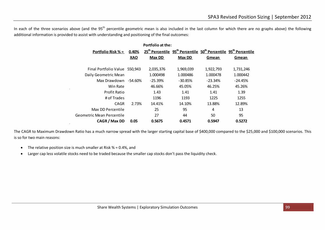
SPA3 Revised Position Sizing | September 2012
Share Wealth Systems | Exploratory Simulation Outcomes 99
In each of the three scenarios above (and the 95th percentile geometric mean is also included in the last column for which there are no graphs above) the following additional information is provided to assist with understanding and positioning of the final outcomes:
The CAGR to Maximum Drawdown Ratio has a much narrow spread with the larger starting capital base of $400,000 compared to the $25,000 and $100,000 scenarios. This is so for two main reasons:
• The relative position size is much smaller at Risk % = 0.4%, and • Larger cap less volatile stocks need to be traded because the smaller cap stocks don’t pass the liquidity check.
Portfolio at the:Portfolio Risk % = 0.40% 25th Percentile 95th Percentile 50th Percentile 95th Percentile
XAO Max DD Max DD Gmean Gmean
Final Portfolio Value 550,943 2,035,376 1,969,039 1,922,793 1,731,246Daily Geometric Mean 1.000498 1.000486 1.000478 1.000442
Max Drawdown -54.60% -25.39% -30.85% -23.34% -24.45%Win Rate 46.66% 45.05% 46.25% 45.26%
Profit Ratio 1.43 1.41 1.41 1.39# of Trades 1196 1193 1225 1255
CAGR 2.73% 14.41% 14.10% 13.88% 12.89%Max DD Percentile 25 95 4 13
Geometric Mean Percentile 27 44 50 95CAGR / Max DD 0.05 0.5675 0.4571 0.5947 0.5272

SPA3 Revised Position Sizing | September 2012
Share Wealth Systems | Exploratory Simulation Outcomes 100
11.3 Portfolio Simulated Equity Curves and Box Plots for SIROC 13 5 5 – Close immediately
The simulation runs in this section use the Market Risk rule that closes all open trades immediately, on the next trading day, when the market turns to High Risk.
11.3.1 25k Charts: SIROC 130505, No Liquidity Check, $9.90 or 0.1% Brokerage
This particular simulation has no liquidity check which means that any trade that met the SPA3 entry criteria could be entered regardless of how illiquid the trade. Whilst unrealistic, this simulation has been run and included in the White Paper to show a base case against which to compare simulations that do include liquidity checks.
The six straw-broom charts have been simulated using the following Portfolio Risk % to calculate the position sizes, in order:
1. Run 859 0.2% Portfolio Risk %. 2. Run 860 0.3%. 3. Run 861 0.4%. 4. Run 862 0.5%. 5. Run 863 0.6%. 6. Run 864 0.8% 7. Run 865 1.0% 8. Run 8661.5% 9. Run 867 2% 10. Run 868 3%

SPA3 Revised Position Sizing | September 2012
Share Wealth Systems | Exploratory Simulation Outcomes 101

SPA3 Revised Position Sizing | September 2012
Share Wealth Systems | Exploratory Simulation Outcomes 102

SPA3 Revised Position Sizing | September 2012
Share Wealth Systems | Exploratory Simulation Outcomes 103

SPA3 Revised Position Sizing | September 2012
Share Wealth Systems | Exploratory Simulation Outcomes 104
0
500
1000
1500
2000
2500
0.2 0.3 0.4 0.5 0.6 0.8 1.0 1.5 2.0 3.0
Risk %
Portfolio Performance Index
200101-201201, XASX SIROC 130505 25k Liq00 B9.90,0.1 (Risks) CI
0.5
0.6
0.7
0.8
0.9
1.0
1.1
1.2
0.2 0.3 0.4 0.5 0.6 0.8 1.0 1.5 2.0 3.0
Risk %
Downside Deviation Factor
200101-201201, XASX SIROC 130505 25k Liq00 B9.90,0.1 (Risks) CI
1
1.0001
1.0002
1.0003
1.0004
1.0005
1.0006
1.0007
1.0008
1.0009
1.001
0.2 0.3 0.4 0.5 0.6 0.8 1.0 1.5 2.0 3.0
Risk %
Daily Geometric Mean
200101-201201, XASX SIROC 130505 25k Liq00 B9.90,0.1 (Risks) CI
0
10
20
30
40
50
60
0.2 0.3 0.4 0.5 0.6 0.8 1.0 1.5 2.0 3.0
Risk %
Maximum Drawdown (%)
200101-201201, XASX SIROC 130505 25k Liq00 B9.90,0.1 (Risks) CI

SPA3 Revised Position Sizing | September 2012
Share Wealth Systems | Exploratory Simulation Outcomes 105
20
25
30
35
40
45
50
55
60
0.2 0.3 0.4 0.5 0.6 0.8 1.0 1.5 2.0 3.0
Risk %
Unallocated Equity Deviation (%)
200101-201201, XASX SIROC 130505 25k Liq00 B9.90,0.1 (Risks) CI
0
500
1,000
1,500
2,000
2,500
3,000
3,500
4,000
0.2 0.3 0.4 0.5 0.6 0.8 1.0 1.5 2.0 3.0
Risk %
Number of Transactions
200101-201201, XASX SIROC 130505 25k Liq00 B9.90,0.1 (Risks) CI
0.4
0.6
0.8
1.0
1.2
1.4
1.6
1.8
2.0
0.2 0.3 0.4 0.5 0.6 0.8 1.0 1.5 2.0 3.0
Risk %
Profit Ratio
200101-201201, XASX SIROC 130505 25k Liq00 B9.90,0.1 (Risks) CI
30
35
40
45
50
55
0.2 0.3 0.4 0.5 0.6 0.8 1.0 1.5 2.0 3.0
Risk %
Win Rate (%)
200101-201201, XASX SIROC 130505 25k Liq00 B9.90,0.1 (Risks) CI

SPA3 Revised Position Sizing | September 2012
Share Wealth Systems | Exploratory Simulation Outcomes 106
11.3.2 25k Charts: SIROC 130505, x10 Liquidity Check, $27.50 or 0.165% Brokerage
The six straw-broom charts have been simulated with the following Portfolio Risk % to calculate the position sizes, in order:
1. Run 889 0.2% Portfolio Risk %. 2. Run 890 0.3%. 3. Run 891 0.4%. 4. Run 892 0.5%. 5. Run 893 0.6%. 6. Run 894 0.8% 7. Run 895 1.0% 8. Run 896 1.5% 9. Run 897 2% 10. Run 898 3%
In this section a liquidity check is introduced compared to the previous section of simulations.
None of these positions sizes would be good enough with which to trade. Note how poorly the smallest position sizes up to 0.6% as the Portfolio Risk % did. This shows complete portfolio meltdown due to paying very high brokerage rates relative to tiny position sizes resulting from a small starting capital.
Just a small increase in position size to 0.8% and then again to 1.0% shows the sensitivity of small portfolios to positions size. All with the same entry and exit signals in individual trades.
You should get the message from these simulations that trading with a small amount of capital has the odds greatly stacked against the active investor when paying a brokerage rate that is relatively too large for the amount of trading capital.
Whilst a Risk % of between 1% and 1.5% provided some hope of the median portfolios outperforming the market benchmark index it would have been a rocky ride over the whole research period. It is NOT recommended to trade with brokerage rates such as these with a small starting capital base.

SPA3 Revised Position Sizing | September 2012
Share Wealth Systems | Exploratory Simulation Outcomes 107

SPA3 Revised Position Sizing | September 2012
Share Wealth Systems | Exploratory Simulation Outcomes 108

SPA3 Revised Position Sizing | September 2012
Share Wealth Systems | Exploratory Simulation Outcomes 109

SPA3 Revised Position Sizing | September 2012
Share Wealth Systems | Exploratory Simulation Outcomes 110
0
500
1000
1500
2000
2500
0.2 0.3 0.4 0.5 0.6 0.8 1.0 1.5 2.0 3.0
Risk %
Portfolio Performance Index
200101-201201, XASX SIROC 130505 25k Liq10 B27.50,0.165 (Risks) CI
0.5
0.6
0.7
0.8
0.9
1.0
1.1
1.2
0.2 0.3 0.4 0.5 0.6 0.8 1.0 1.5 2.0 3.0
Risk %
Downside Deviation Factor
200101-201201, XASX SIROC 130505 25k Liq10 B27.50,0.165 (Risks) CI
1
1.0001
1.0002
1.0003
1.0004
1.0005
1.0006
1.0007
1.0008
1.0009
1.001
0.2 0.3 0.4 0.5 0.6 0.8 1.0 1.5 2.0 3.0
Risk %
Daily Geometric Mean
200101-201201, XASX SIROC 130505 25k Liq10 B27.50,0.165 (Risks) CI
0
10
20
30
40
50
60
0.2 0.3 0.4 0.5 0.6 0.8 1.0 1.5 2.0 3.0
Risk %
Maximum Drawdown (%)
200101-201201, XASX SIROC 130505 25k Liq10 B27.50,0.165 (Risks) CI

SPA3 Revised Position Sizing | September 2012
Share Wealth Systems | Exploratory Simulation Outcomes 111
20
25
30
35
40
45
50
55
60
0.2 0.3 0.4 0.5 0.6 0.8 1.0 1.5 2.0 3.0
Risk %
Unallocated Equity Deviation (%)
200101-201201, XASX SIROC 130505 25k Liq10 B27.50,0.165 (Risks) CI
0
500
1,000
1,500
2,000
2,500
3,000
3,500
4,000
0.2 0.3 0.4 0.5 0.6 0.8 1.0 1.5 2.0 3.0
Risk %
Number of Transactions
200101-201201, XASX SIROC 130505 25k Liq10 B27.50,0.165 (Risks) CI
0.4
0.6
0.8
1.0
1.2
1.4
1.6
1.8
2.0
0.2 0.3 0.4 0.5 0.6 0.8 1.0 1.5 2.0 3.0
Risk %
Profit Ratio
200101-201201, XASX SIROC 130505 25k Liq10 B27.50,0.165 (Risks) CI
30
35
40
45
50
55
0.2 0.3 0.4 0.5 0.6 0.8 1.0 1.5 2.0 3.0
Risk %
Win Rate (%)
200101-201201, XASX SIROC 130505 25k Liq10 B27.50,0.165 (Risks) CI

SPA3 Revised Position Sizing | September 2012
Share Wealth Systems | Exploratory Simulation Outcomes 112
11.3.3 25k Charts: SIROC 130505, x10 Liquidity Check, $19.95 or 0.1% Brokerage
The seven straw-broom charts have been simulated with the following Portfolio Risk % to calculate the position sizes, in order:
1. Run 879 0.2% Portfolio Risk %. 2. Run 880 0.3%. 3. Run 881 0.4%. 4. Run 882 0.5%. 5. Run 883 0.6%. 6. Run 884 0.8% 7. Run 885 1.0% 8. Run 886 1.5% 9. Run 887 2% 10. Run 888 3%
Note what a big difference the drop in the minimum brokerage from $27.50 to $19.95 makes when trading with a small starting capital.
The 0.8% - 1.5% Portfolio Risk % would stand good odds of outperforming the market benchmark with relatively low drawdown. However, the variation of equity curve outcomes are still quite wide meaning that portfolio outcomes would be more sensitive to trading errors and / or trade selection.
It is recommended to trade with lower brokerage levels than $19.95 for a small portfolio.
It is important to understand that with a small portfolio value the majority of trades are charged the minimum brokerage rate of $19.95 until the portfolio gets large enough to get to the 0.1% brokerage level. This is why small portfolios are so sensitive to the minimum brokerage rate. A position size > $19,950 would be required for the 0.1% rate to kick in and all positions < $19,950 would attract the $19.95 brokerage rate, even a trade with a $2,000 position size where the brokerage rate would be 0.9975% and the round trip would 1.995%, say 2%, meaning that trades, on average, would need to move by at least double to triple this to make headway.
Even a rate at $15 or $12 will make a big difference. Raising the starting capital to $30,000, $35,000 or $40,000 will also make a big difference, if using a brokerage rate of $19.95.
Be very aware of these sensitivities with a small portfolio starting base.

SPA3 Revised Position Sizing | September 2012
Share Wealth Systems | Exploratory Simulation Outcomes 113

SPA3 Revised Position Sizing | September 2012
Share Wealth Systems | Exploratory Simulation Outcomes 114

SPA3 Revised Position Sizing | September 2012
Share Wealth Systems | Exploratory Simulation Outcomes 115

SPA3 Revised Position Sizing | September 2012
Share Wealth Systems | Exploratory Simulation Outcomes 116
0
500
1000
1500
2000
2500
0.2 0.3 0.4 0.5 0.6 0.8 1.0 1.5 2.0 3.0
Risk %
Portfolio Performance Index
200101-201201, XASX SIROC 130505 25k Liq10 B19.95,0.1 (Risks) CI
0.5
0.6
0.7
0.8
0.9
1.0
1.1
1.2
0.2 0.3 0.4 0.5 0.6 0.8 1.0 1.5 2.0 3.0
Risk %
Downside Deviation Factor
200101-201201, XASX SIROC 130505 25k Liq10 B19.95,0.1 (Risks) CI
1
1.0001
1.0002
1.0003
1.0004
1.0005
1.0006
1.0007
1.0008
1.0009
1.001
0.2 0.3 0.4 0.5 0.6 0.8 1.0 1.5 2.0 3.0
Risk %
Daily Geometric Mean
200101-201201, XASX SIROC 130505 25k Liq10 B19.95,0.1 (Risks) CI
0
10
20
30
40
50
60
0.2 0.3 0.4 0.5 0.6 0.8 1.0 1.5 2.0 3.0
Risk %
Maximum Drawdown (%)
200101-201201, XASX SIROC 130505 25k Liq10 B19.95,0.1 (Risks) CI

SPA3 Revised Position Sizing | September 2012
Share Wealth Systems | Exploratory Simulation Outcomes 117
20
25
30
35
40
45
50
55
60
0.2 0.3 0.4 0.5 0.6 0.8 1.0 1.5 2.0 3.0
Risk %
Unallocated Equity Deviation (%)
200101-201201, XASX SIROC 130505 25k Liq10 B19.95,0.1 (Risks) CI
0
500
1,000
1,500
2,000
2,500
3,000
3,500
4,000
0.2 0.3 0.4 0.5 0.6 0.8 1.0 1.5 2.0 3.0
Risk %
Number of Transactions
200101-201201, XASX SIROC 130505 25k Liq10 B19.95,0.1 (Risks) CI
0.4
0.6
0.8
1.0
1.2
1.4
1.6
1.8
2.0
0.2 0.3 0.4 0.5 0.6 0.8 1.0 1.5 2.0 3.0
Risk %
Profit Ratio
200101-201201, XASX SIROC 130505 25k Liq10 B19.95,0.1 (Risks) CI
30
35
40
45
50
55
0.2 0.3 0.4 0.5 0.6 0.8 1.0 1.5 2.0 3.0
Risk %
Win Rate (%)
200101-201201, XASX SIROC 130505 25k Liq10 B19.95,0.1 (Risks) CI

SPA3 Revised Position Sizing | September 2012
Share Wealth Systems | Exploratory Simulation Outcomes 118
11.3.4 25k Charts: SIROC 130505, x10 Liquidity Check, $9.90 or 0.1% Brokerage
The ten straw-broom charts have been simulated with the following Portfolio Risk % to calculate the position sizes, in order:
1. Run 869 0.2% Portfolio Risk %. 2. Run 870 0.3%. 3. Run 871 0.4%. 4. Run 872 0.5%. 5. Run 873 0.6%. 6. Run 874 0.8% 7. Run 875 1.0% 8. Run 876 1.5% 9. Run 877 2% 10. Run 878 3%
Note how poor the equity curves were for the Risk % position sizes below 1% and 0.8% in the previous two $25,000 portfolio sections, due to high brokerage rates relative to the small portfolio value.
For small portfolio starting capital using a broker with a low minimum brokerage rate makes a huge difference to returns, drawdown and compounding by being able to use your money for re-investing rather than paying that money away in brokerage. As the SPA3 Reference Manual highlights, for small starting capitals, the majority of profits that the SPA3 Edge generates are paid in brokerage fees.
The portfolio meltdown caused purely by brokerage is largely removed when using a minimum brokerage rate as low as $9.90. The SPA3 active investor gets to keep far more of the profits generated by the SPA3 Edge. Obviously using a minimum brokerage rate of $15 or 0.1%, or $16.50 or 0.11% can work with a small portfolio and would be far better than $19.95 but the lower that the minimum rate the better, and this is especially so with a small portfolio.
The best Risk % for position sizes using this portfolio scenario are 0.4% - 0.8%.
Risk % 0.2% and 0.3% should be avoided.
This set of simulations with SIROC 13 5 5 ‘close immediately’ can be compared to the simulations with SIROC 13 5 5 ‘leave trades open’ in section 11.4.3 on page 178.

SPA3 Revised Position Sizing | September 2012
Share Wealth Systems | Exploratory Simulation Outcomes 119

SPA3 Revised Position Sizing | September 2012
Share Wealth Systems | Exploratory Simulation Outcomes 120

SPA3 Revised Position Sizing | September 2012
Share Wealth Systems | Exploratory Simulation Outcomes 121
Summary:
• Risk % 0.2% would fail totally due to position sizes being far too small for even the lowest brokerage rate available in Australia at this time, i.e. portfolio meltdown. o This Risk %’s would produce such small positions sizes because the portfolio starting capital is low at $25,000.
• Using the equity curve outcomes above and the box plots below: o Risk % of 1.5% should not be exceeded. o A Risk % under 0.4% should not be used.
In the box plots that follow note the following:
• There is a 95% chance of having a maximum drawdown of less than 20% when trading this portfolio scenario with a Risk % of 0.4%. • There is a 75% chance of having a maximum drawdown of less than 20% when trading this portfolio scenario with a Risk % of 0.5%. • There is a 95% chance of having a maximum drawdown of less than 25% when trading this portfolio scenario with a Risk % of 0.8%. • At Risk % of 0.8% the PPI and Geometric Mean rise dramatically meaning that the potential for outperformance is far greater with this position size provided that a
little more risk can be tolerated.

SPA3 Revised Position Sizing | September 2012
Share Wealth Systems | Exploratory Simulation Outcomes 122
0
500
1000
1500
2000
2500
0.2 0.3 0.4 0.5 0.6 0.8 1.0 1.5 2.0 3.0
Risk %
Portfolio Performance Index
200101-201201, XASX SIROC 130505 25k Liq10 B9.90,0.1 (Risks) CI
0.5
0.6
0.7
0.8
0.9
1.0
1.1
1.2
0.2 0.3 0.4 0.5 0.6 0.8 1.0 1.5 2.0 3.0
Risk %
Downside Deviation Factor
200101-201201, XASX SIROC 130505 25k Liq10 B9.90,0.1 (Risks) CI
1
1.0001
1.0002
1.0003
1.0004
1.0005
1.0006
1.0007
1.0008
1.0009
1.001
0.2 0.3 0.4 0.5 0.6 0.8 1.0 1.5 2.0 3.0
Risk %
Daily Geometric Mean
200101-201201, XASX SIROC 130505 25k Liq10 B9.90,0.1 (Risks) CI
0
10
20
30
40
50
60
0.2 0.3 0.4 0.5 0.6 0.8 1.0 1.5 2.0 3.0
Risk %
Maximum Drawdown (%)
200101-201201, XASX SIROC 130505 25k Liq10 B9.90,0.1 (Risks) CI

SPA3 Revised Position Sizing | September 2012
Share Wealth Systems | Exploratory Simulation Outcomes 123
20
25
30
35
40
45
50
55
60
0.2 0.3 0.4 0.5 0.6 0.8 1.0 1.5 2.0 3.0
Risk %
Unallocated Equity Deviation (%)
200101-201201, XASX SIROC 130505 25k Liq10 B9.90,0.1 (Risks) CI
0
500
1,000
1,500
2,000
2,500
3,000
3,500
4,000
0.2 0.3 0.4 0.5 0.6 0.8 1.0 1.5 2.0 3.0
Risk %
Number of Transactions
200101-201201, XASX SIROC 130505 25k Liq10 B9.90,0.1 (Risks) CI
0.4
0.6
0.8
1.0
1.2
1.4
1.6
1.8
2.0
0.2 0.3 0.4 0.5 0.6 0.8 1.0 1.5 2.0 3.0
Risk %
Profit Ratio
200101-201201, XASX SIROC 130505 25k Liq10 B9.90,0.1 (Risks) CI
30
35
40
45
50
55
0.2 0.3 0.4 0.5 0.6 0.8 1.0 1.5 2.0 3.0
Risk %
Win Rate (%)
200101-201201, XASX SIROC 130505 25k Liq10 B9.90,0.1 (Risks) CI

SPA3 Revised Position Sizing | September 2012
Share Wealth Systems | Exploratory Simulation Outcomes 124
11.3.4.1 Individual Equity Curves & Underwater Equity Curves
Using the above graphical output, assume a Portfolio Risk % of 0.8%. From run 874 above we know that there were 1000 unique equity curves generated by selecting trades randomly when there was available capital, according to the SPA3 entry & exit criteria and the risk management & position sizing rules. We have selected two individual portfolios from the 1000 portfolio simulation that may be representative of a potential equity curve outcome to assist positioning how a SPA3 trader’s equity curve may eventuate, provided that the rules are followed in a mechanical manner:
1. The median geometrical mean. This is the portfolio that ended at the 50th percentile, that is, the middle line on the box plot. Half of the 1000 portfolios would have performed better and half worse as at the end of the simulation period in January 2012. This does not mean that it would have been the median portfolio all the way through the simulation period, just at the completion date of the simulation period. This the first set of graphs.
2. The maximum drawdown at the 95th percentile. This is the portfolio that had 95% of the 1000 portfolios with a better (lower or shallower) maximum drawdown and 5% that had worse maximum drawdowns. It came 95th using Maximum Drawdown as a single metric. This the second set of graphs.
The following graphs are provided for each of the two equity curves:
5. The mark-to-market equity curve in arithmetic and log mode. The red plot is the All Ordinaries Index. 6. The % drawdown underwater equity curve vertical axis is scaled according to the maximum drawdown reached in the life of the portfolio. 7. The underwater curve for the portfolio (black shadow) compared to the underwater curve for the All Ordinaries Index (red shadow). 8. The open positions through the life of the portfolio. The periods where they are no open positions are when the portfolio was 100% in cash during High Market Risk
periods, according to Risk Profile 1.

SPA3 Revised Position Sizing | September 2012
Share Wealth Systems | Exploratory Simulation Outcomes 125

SPA3 Revised Position Sizing | September 2012
Share Wealth Systems | Exploratory Simulation Outcomes 126

SPA3 Revised Position Sizing | September 2012
Share Wealth Systems | Exploratory Simulation Outcomes 127

SPA3 Revised Position Sizing | September 2012
Share Wealth Systems | Exploratory Simulation Outcomes 128
In each of the three scenarios above (and the 95th percentile geometric mean is also included in the last column for which there are no graphs above) the following additional information is provided to assist with understanding and positioning of the final outcomes:
The SIROC 130505 results look somewhat better than the SIROC 21 8 results in section 11.2.3.1 on page 53.
Portfolio at the:Portfolio Risk % = 0.80% 25th Percentile 95th Percentile 50th Percentile 95th Percentile
XAO Max DD Max DD Gmean Gmean
Final Portfolio Value 34,434 298,625 179,490 254,335 164,540Daily Geometric Mean 1.000749 1.000582 1.000699 1.000558
Max Drawdown -54.60% -18.38% -24.90% -17.70% -23.26%Win Rate 47.38% 45.03% 46.40% 45.26%
Profit Ratio 1.66 1.47 1.56 1.43# of Trades 755 764 783 755
CAGR 2.73% 22.79% 17.72% 21.17% 16.88%Max DD Percentile 25 95 18 87
Geometric Mean Percentile 23 92 50 95CAGR / Max DD 0.05 1.2399 0.7116 1.1960 0.7257

SPA3 Revised Position Sizing | September 2012
Share Wealth Systems | Exploratory Simulation Outcomes 129
11.3.5 100k Charts: SIROC 130505, No Liquidity Check, $27.50 or 0.165% Brokerage
Again, this “no liquidity check” simulation does not reflect a realistic trading environment and is provided as a benchmark by which to compare to simulations runs that do include liquidity checks.
1. Run 899 0.2% Portfolio Risk %. 2. Run 900 0.3%. 3. Run 901 0.4%. 4. Run 902 0.5%. 5. Run 903 0.6%. 6. Run 904 0.8%. 7. Run 905 1%. 8. Run 906 1.5%. 9. Run 907 2%. 10. Run 908 3%.

SPA3 Revised Position Sizing | September 2012
Share Wealth Systems | Exploratory Simulation Outcomes 130
0
500
1000
1500
2000
2500
0.2 0.3 0.4 0.5 0.6 0.8 1.0 1.5 2.0 3.0
Risk %
Portfolio Performance Index
200101-201201, XASX SIROC 130505 100k Liq00 B27.50,0.165 (Risks) CI
0.5
0.6
0.7
0.8
0.9
1.0
1.1
1.2
0.2 0.3 0.4 0.5 0.6 0.8 1.0 1.5 2.0 3.0
Risk %
Downside Deviation Factor
200101-201201, XASX SIROC 130505 100k Liq00 B27.50,0.165 (Risks) CI
1
1.0001
1.0002
1.0003
1.0004
1.0005
1.0006
1.0007
1.0008
1.0009
1.001
0.2 0.3 0.4 0.5 0.6 0.8 1.0 1.5 2.0 3.0
Risk %
Daily Geometric Mean
200101-201201, XASX SIROC 130505 100k Liq00 B27.50,0.165 (Risks) CI
0
10
20
30
40
50
60
0.2 0.3 0.4 0.5 0.6 0.8 1.0 1.5 2.0 3.0
Risk %
Maximum Drawdown (%)
200101-201201, XASX SIROC 130505 100k Liq00 B27.50,0.165 (Risks) CI

SPA3 Revised Position Sizing | September 2012
Share Wealth Systems | Exploratory Simulation Outcomes 131
20
25
30
35
40
45
50
55
60
0.2 0.3 0.4 0.5 0.6 0.8 1.0 1.5 2.0 3.0
Risk %
Unallocated Equity Deviation (%)
200101-201201, XASX SIROC 130505 100k Liq00 B27.50,0.165 (Risks) CI
0
500
1,000
1,500
2,000
2,500
3,000
3,500
4,000
0.2 0.3 0.4 0.5 0.6 0.8 1.0 1.5 2.0 3.0
Risk %
Number of Transactions
200101-201201, XASX SIROC 130505 100k Liq00 B27.50,0.165 (Risks) CI
0.4
0.6
0.8
1.0
1.2
1.4
1.6
1.8
2.0
0.2 0.3 0.4 0.5 0.6 0.8 1.0 1.5 2.0 3.0
Risk %
Profit Ratio
200101-201201, XASX SIROC 130505 100k Liq00 B27.50,0.165 (Risks) CI
30
35
40
45
50
55
0.2 0.3 0.4 0.5 0.6 0.8 1.0 1.5 2.0 3.0
Risk %
Win Rate (%)
200101-201201, XASX SIROC 130505 100k Liq00 B27.50,0.165 (Risks) CI

SPA3 Revised Position Sizing | September 2012
Share Wealth Systems | Exploratory Simulation Outcomes 132
11.3.6 100k Charts: SIROC 130505, x5 Liquidity Check, $27.50 or 0.165% Brokerage
1. Run 909 0.2% Portfolio Risk %. 2. Run 910 0.3%. 3. Run 911 0.4%. 4. Run 912 0.5%. 5. Run 913 0.6%. 6. Run 914 0.8%. 7. Run 915 1%. 8. Run 916 1.5%. 9. Run 917 2%. 10. Run 918 3%.

SPA3 Revised Position Sizing | September 2012
Share Wealth Systems | Exploratory Simulation Outcomes 133

SPA3 Revised Position Sizing | September 2012
Share Wealth Systems | Exploratory Simulation Outcomes 134

SPA3 Revised Position Sizing | September 2012
Share Wealth Systems | Exploratory Simulation Outcomes 135
Summary:
• Risk % 0.2% would be too small a position size for this portfolio scenario. Brokerage would be the reason. • Using the equity curve outcomes above and the box plots below:
o Risk % of 1.0% should not be exceeded. o A Risk % under 0.3% should not be used. o 0.3% should only be used if keeping the maximum drawdown to a minimum is the main aim.

SPA3 Revised Position Sizing | September 2012
Share Wealth Systems | Exploratory Simulation Outcomes 136
0
500
1000
1500
2000
2500
0.2 0.3 0.4 0.5 0.6 0.8 1.0 1.5 2.0 3.0
Risk %
Portfolio Performance Index
200101-201201, XASX SIROC 130505 100k Liq05 B27.50,0.165 (Risks) CI
0.5
0.6
0.7
0.8
0.9
1.0
1.1
1.2
0.2 0.3 0.4 0.5 0.6 0.8 1.0 1.5 2.0 3.0
Risk %
Downside Deviation Factor
200101-201201, XASX SIROC 130505 100k Liq05 B27.50,0.165 (Risks) CI
1
1.0001
1.0002
1.0003
1.0004
1.0005
1.0006
1.0007
1.0008
1.0009
1.001
0.2 0.3 0.4 0.5 0.6 0.8 1.0 1.5 2.0 3.0
Risk %
Daily Geometric Mean
200101-201201, XASX SIROC 130505 100k Liq05 B27.50,0.165 (Risks) CI
0
10
20
30
40
50
60
0.2 0.3 0.4 0.5 0.6 0.8 1.0 1.5 2.0 3.0
Risk %
Maximum Drawdown (%)
200101-201201, XASX SIROC 130505 100k Liq05 B27.50,0.165 (Risks) CI

SPA3 Revised Position Sizing | September 2012
Share Wealth Systems | Exploratory Simulation Outcomes 137
20
25
30
35
40
45
50
55
60
0.2 0.3 0.4 0.5 0.6 0.8 1.0 1.5 2.0 3.0
Risk %
Unallocated Equity Deviation (%)
200101-201201, XASX SIROC 130505 100k Liq05 B27.50,0.165 (Risks) CI
0
500
1,000
1,500
2,000
2,500
3,000
3,500
4,000
0.2 0.3 0.4 0.5 0.6 0.8 1.0 1.5 2.0 3.0
Risk %
Number of Transactions
200101-201201, XASX SIROC 130505 100k Liq05 B27.50,0.165 (Risks) CI
0.4
0.6
0.8
1.0
1.2
1.4
1.6
1.8
2.0
0.2 0.3 0.4 0.5 0.6 0.8 1.0 1.5 2.0 3.0
Risk %
Profit Ratio
200101-201201, XASX SIROC 130505 100k Liq05 B27.50,0.165 (Risks) CI
30
35
40
45
50
55
0.2 0.3 0.4 0.5 0.6 0.8 1.0 1.5 2.0 3.0
Risk %
Win Rate (%)
200101-201201, XASX SIROC 130505 100k Liq05 B27.50,0.165 (Risks) CI

SPA3 Revised Position Sizing | September 2012
Share Wealth Systems | Exploratory Simulation Outcomes 138
11.3.7 100k Charts: SIROC 130505, x10 Liquidity Check, $27.50 or 0.165% Brokerage
1. Run 929 0.2% Portfolio Risk %. 2. Run 930 0.3%. 3. Run 931 0.4%. 4. Run 932 0.5%. 5. Run 933 0.6%. 6. Run 934 0.8%. 7. Run 935 1%. 8. Run 936 1.5%. 9. Run 937 2%. 10. Run 938 3%.
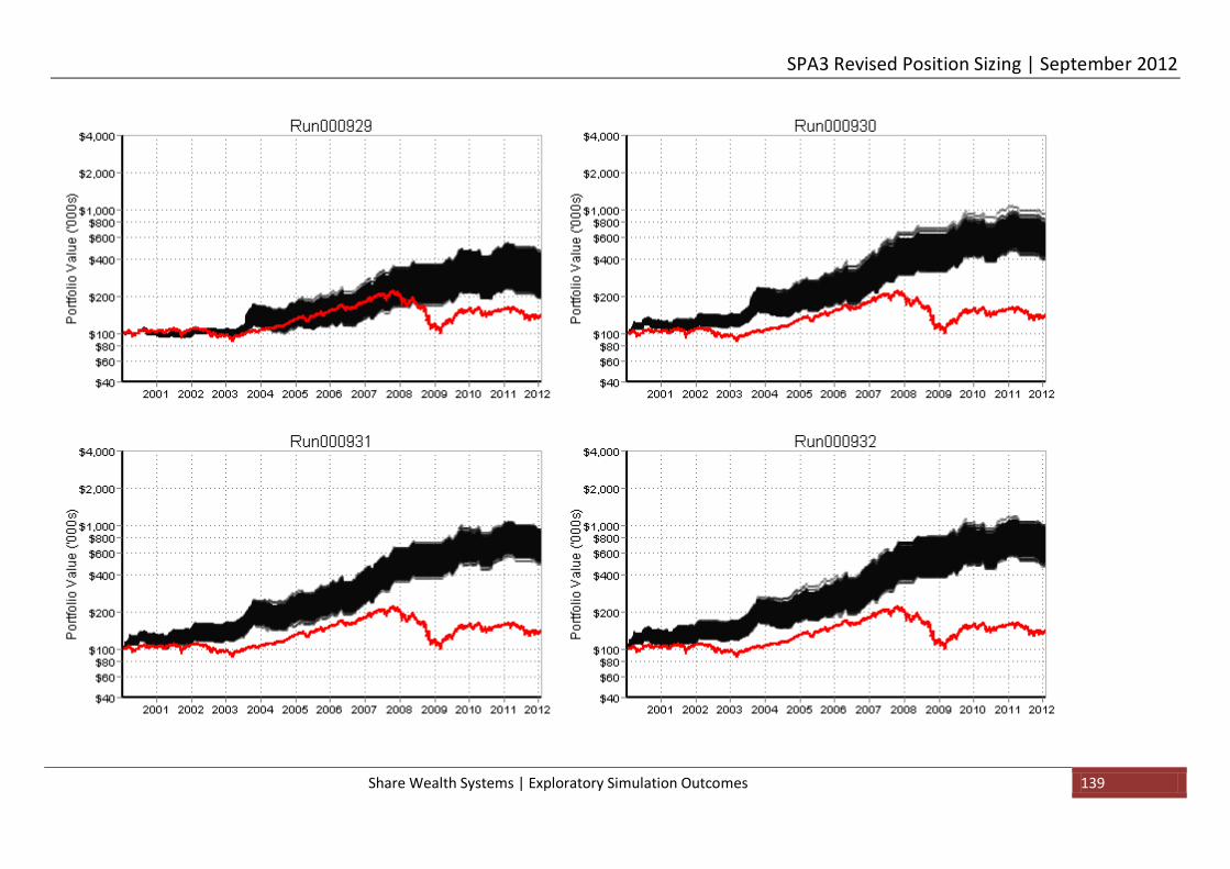
SPA3 Revised Position Sizing | September 2012
Share Wealth Systems | Exploratory Simulation Outcomes 139
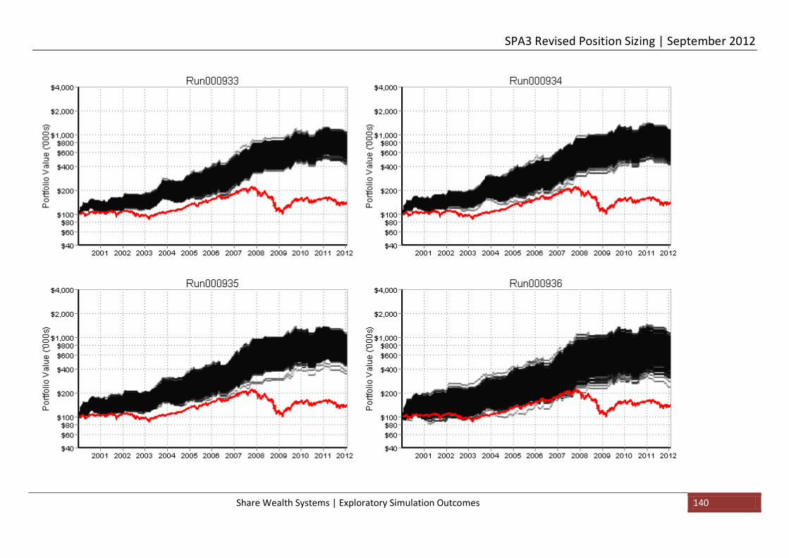
SPA3 Revised Position Sizing | September 2012
Share Wealth Systems | Exploratory Simulation Outcomes 140

SPA3 Revised Position Sizing | September 2012
Share Wealth Systems | Exploratory Simulation Outcomes 141
Summary:
• Risk % 0.2% would be too small a position size for this portfolio scenario. Brokerage would be the reason. • Using the equity curve outcomes above and the box plots below:
o Risk % of 1.0% should not be exceeded. o A Risk % under 0.3% should not be used. o 0.3% should only be used if keeping the maximum drawdown to a minimum is the main aim. Note too the large number of trades at this position size.

SPA3 Revised Position Sizing | September 2012
Share Wealth Systems | Exploratory Simulation Outcomes 142
0
500
1000
1500
2000
2500
0.2 0.3 0.4 0.5 0.6 0.8 1.0 1.5 2.0 3.0
Risk %
Portfolio Performance Index
200101-201201, XASX SIROC 130505 100k Liq10 B27.50,0.165 (Risks) CI
0.5
0.6
0.7
0.8
0.9
1.0
1.1
1.2
0.2 0.3 0.4 0.5 0.6 0.8 1.0 1.5 2.0 3.0
Risk %
Downside Deviation Factor
200101-201201, XASX SIROC 130505 100k Liq10 B27.50,0.165 (Risks) CI
1
1.0001
1.0002
1.0003
1.0004
1.0005
1.0006
1.0007
1.0008
1.0009
1.001
0.2 0.3 0.4 0.5 0.6 0.8 1.0 1.5 2.0 3.0
Risk %
Daily Geometric Mean
200101-201201, XASX SIROC 130505 100k Liq10 B27.50,0.165 (Risks) CI
0
10
20
30
40
50
60
0.2 0.3 0.4 0.5 0.6 0.8 1.0 1.5 2.0 3.0
Risk %
Maximum Drawdown (%)
200101-201201, XASX SIROC 130505 100k Liq10 B27.50,0.165 (Risks) CI

SPA3 Revised Position Sizing | September 2012
Share Wealth Systems | Exploratory Simulation Outcomes 143
20
25
30
35
40
45
50
55
60
0.2 0.3 0.4 0.5 0.6 0.8 1.0 1.5 2.0 3.0
Risk %
Unallocated Equity Deviation (%)
200101-201201, XASX SIROC 130505 100k Liq10 B27.50,0.165 (Risks) CI
0
500
1,000
1,500
2,000
2,500
3,000
3,500
4,000
0.2 0.3 0.4 0.5 0.6 0.8 1.0 1.5 2.0 3.0
Risk %
Number of Transactions
200101-201201, XASX SIROC 130505 100k Liq10 B27.50,0.165 (Risks) CI
0.4
0.6
0.8
1.0
1.2
1.4
1.6
1.8
2.0
0.2 0.3 0.4 0.5 0.6 0.8 1.0 1.5 2.0 3.0
Risk %
Profit Ratio
200101-201201, XASX SIROC 130505 100k Liq10 B27.50,0.165 (Risks) CI
30
35
40
45
50
55
0.2 0.3 0.4 0.5 0.6 0.8 1.0 1.5 2.0 3.0
Risk %
Win Rate (%)
200101-201201, XASX SIROC 130505 100k Liq10 B27.50,0.165 (Risks) CI

SPA3 Revised Position Sizing | September 2012
Share Wealth Systems | Exploratory Simulation Outcomes 144
11.3.8 100k Charts: SIROC 130505, x5 Liquidity Check, $9.90 or 0.1% Brokerage
1. Run 919 0.2% Portfolio Risk %. 2. Run 920 0.3%. 3. Run 921 0.4%. 4. Run 922 0.5%. 5. Run 923 0.6%. 6. Run 924 0.8%. 7. Run 925 1%. 8. Run 926 1.5%. 9. Run 927 2%. 10. Run 928 3%.

SPA3 Revised Position Sizing | September 2012
Share Wealth Systems | Exploratory Simulation Outcomes 145

SPA3 Revised Position Sizing | September 2012
Share Wealth Systems | Exploratory Simulation Outcomes 146

SPA3 Revised Position Sizing | September 2012
Share Wealth Systems | Exploratory Simulation Outcomes 147
Some comments about this portfolio scenario simulation:
• The 0.2% Risk % may look like an excellent outcome when starting with $100,000 on a low brokerage rate, and its does look fantastic, however note the high number of transactions. 5100 transactions over 12 years = 2550 trades = an average of 212.5 a year = 17.7 a month. For this effort the reward is a 95% chance of having a maximum drawdown of less that 15% meaning that all other drawdowns through the life of the portfolio would be even less.
Summary:
• Using the equity curve outcomes above and the box plots below: o Risk % of 1.0% should not be exceeded. o Risk % of 0.2% can be used. o 0.2% should only be used if keeping the maximum drawdown to a minimum is the main aim. Note too, the large number of trades at this position size.

SPA3 Revised Position Sizing | September 2012
Share Wealth Systems | Exploratory Simulation Outcomes 148
0
500
1000
1500
2000
2500
0.2 0.3 0.4 0.5 0.6 0.8 1.0 1.5 2.0 3.0
Risk %
Portfolio Performance Index
200101-201201, XASX SIROC 130505 100k Liq05 B9.90,0.1 (Risks) CI
0.5
0.6
0.7
0.8
0.9
1.0
1.1
1.2
0.2 0.3 0.4 0.5 0.6 0.8 1.0 1.5 2.0 3.0
Risk %
Downside Deviation Factor
200101-201201, XASX SIROC 130505 100k Liq05 B9.90,0.1 (Risks) CI
1
1.0001
1.0002
1.0003
1.0004
1.0005
1.0006
1.0007
1.0008
1.0009
1.001
0.2 0.3 0.4 0.5 0.6 0.8 1.0 1.5 2.0 3.0
Risk %
Daily Geometric Mean
200101-201201, XASX SIROC 130505 100k Liq05 B9.90,0.1 (Risks) CI
0
10
20
30
40
50
60
0.2 0.3 0.4 0.5 0.6 0.8 1.0 1.5 2.0 3.0
Risk %
Maximum Drawdown (%)
200101-201201, XASX SIROC 130505 100k Liq05 B9.90,0.1 (Risks) CI

SPA3 Revised Position Sizing | September 2012
Share Wealth Systems | Exploratory Simulation Outcomes 149
20
25
30
35
40
45
50
55
60
0.2 0.3 0.4 0.5 0.6 0.8 1.0 1.5 2.0 3.0
Risk %
Unallocated Equity Deviation (%)
200101-201201, XASX SIROC 130505 100k Liq05 B9.90,0.1 (Risks) CI
0
500
1,000
1,500
2,000
2,500
3,000
3,500
4,000
0.2 0.3 0.4 0.5 0.6 0.8 1.0 1.5 2.0 3.0
Risk %
Number of Transactions
200101-201201, XASX SIROC 130505 100k Liq05 B9.90,0.1 (Risks) CI
0.4
0.6
0.8
1.0
1.2
1.4
1.6
1.8
2.0
0.2 0.3 0.4 0.5 0.6 0.8 1.0 1.5 2.0 3.0
Risk %
Profit Ratio
200101-201201, XASX SIROC 130505 100k Liq05 B9.90,0.1 (Risks) CI
30
35
40
45
50
55
0.2 0.3 0.4 0.5 0.6 0.8 1.0 1.5 2.0 3.0
Risk %
Win Rate (%)
200101-201201, XASX SIROC 130505 100k Liq05 B9.90,0.1 (Risks) CI

SPA3 Revised Position Sizing | September 2012
Share Wealth Systems | Exploratory Simulation Outcomes 150
11.3.9 100k Charts: SIROC 130505, x10 Liquidity Check, $9.90 or 0.1% Brokerage
1. Run 939 0.2% Portfolio Risk %. 2. Run 940 0.3%. 3. Run 941 0.4%. 4. Run 942 0.5%. 5. Run 943 0.6%. 6. Run 944 0.8%. 7. Run 945 1%. 8. Run 946 1.5%. 9. Run 947 2%. 10. Run 948 3%.
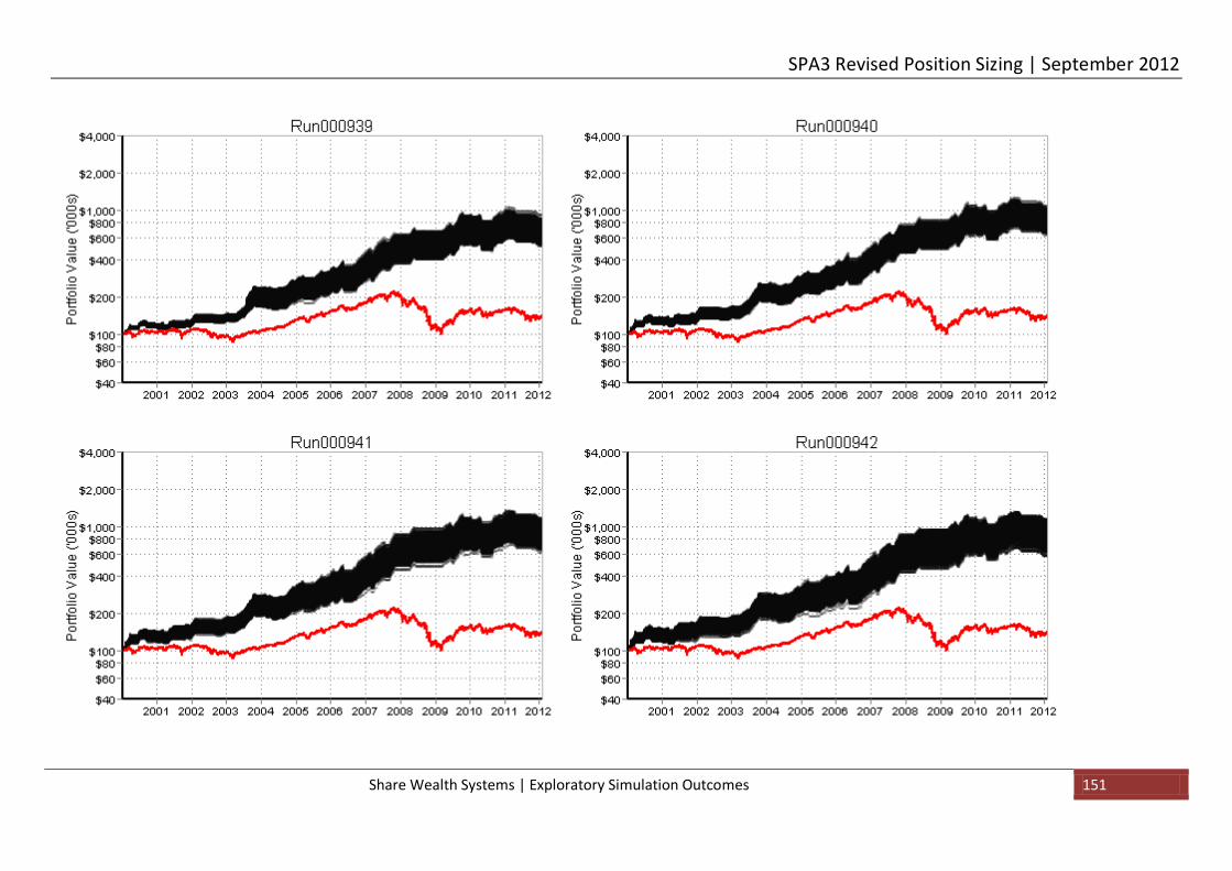
SPA3 Revised Position Sizing | September 2012
Share Wealth Systems | Exploratory Simulation Outcomes 151

SPA3 Revised Position Sizing | September 2012
Share Wealth Systems | Exploratory Simulation Outcomes 152

SPA3 Revised Position Sizing | September 2012
Share Wealth Systems | Exploratory Simulation Outcomes 153
Summary:
• Using the equity curve outcomes above and the box plots below: o Risk % of 1.0% should not be exceeded. o Risk % of 0.2% can be used. o 0.4% has the lowest maximum drawdown box plot as well as the highest PPI and geometric mean.
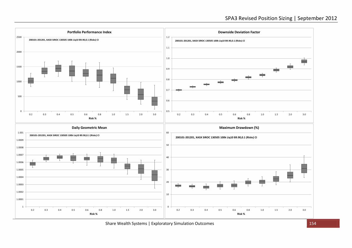
SPA3 Revised Position Sizing | September 2012
Share Wealth Systems | Exploratory Simulation Outcomes 154
0
500
1000
1500
2000
2500
0.2 0.3 0.4 0.5 0.6 0.8 1.0 1.5 2.0 3.0
Risk %
Portfolio Performance Index
200101-201201, XASX SIROC 130505 100k Liq10 B9.90,0.1 (Risks) CI
0.5
0.6
0.7
0.8
0.9
1.0
1.1
1.2
0.2 0.3 0.4 0.5 0.6 0.8 1.0 1.5 2.0 3.0
Risk %
Downside Deviation Factor
200101-201201, XASX SIROC 130505 100k Liq10 B9.90,0.1 (Risks) CI
1
1.0001
1.0002
1.0003
1.0004
1.0005
1.0006
1.0007
1.0008
1.0009
1.001
0.2 0.3 0.4 0.5 0.6 0.8 1.0 1.5 2.0 3.0
Risk %
Daily Geometric Mean
200101-201201, XASX SIROC 130505 100k Liq10 B9.90,0.1 (Risks) CI
0
10
20
30
40
50
60
0.2 0.3 0.4 0.5 0.6 0.8 1.0 1.5 2.0 3.0
Risk %
Maximum Drawdown (%)
200101-201201, XASX SIROC 130505 100k Liq10 B9.90,0.1 (Risks) CI

SPA3 Revised Position Sizing | September 2012
Share Wealth Systems | Exploratory Simulation Outcomes 155
20
25
30
35
40
45
50
55
60
0.2 0.3 0.4 0.5 0.6 0.8 1.0 1.5 2.0 3.0
Risk %
Unallocated Equity Deviation (%)
200101-201201, XASX SIROC 130505 100k Liq10 B9.90,0.1 (Risks) CI
0
500
1,000
1,500
2,000
2,500
3,000
3,500
4,000
0.2 0.3 0.4 0.5 0.6 0.8 1.0 1.5 2.0 3.0
Risk %
Number of Transactions
200101-201201, XASX SIROC 130505 100k Liq10 B9.90,0.1 (Risks) CI
0.4
0.6
0.8
1.0
1.2
1.4
1.6
1.8
2.0
0.2 0.3 0.4 0.5 0.6 0.8 1.0 1.5 2.0 3.0
Risk %
Profit Ratio
200101-201201, XASX SIROC 130505 100k Liq10 B9.90,0.1 (Risks) CI
30
35
40
45
50
55
0.2 0.3 0.4 0.5 0.6 0.8 1.0 1.5 2.0 3.0
Risk %
Win Rate (%)
200101-201201, XASX SIROC 130505 100k Liq10 B9.90,0.1 (Risks) CI
SPA3 Revised Position Sizing | September 2012
Share Wealth Systems | Exploratory Simulation Outcomes 156
11.3.10 400k Charts: SIROC 130505, x5 Liquidity Check, $27.50 or 0.165% Brokerage
1. Run 959 0.2% Portfolio Risk %. 2. Run 960 0.3%. 3. Run 961 0.4%. 4. Run 962 0.5%. 5. Run 963 0.6%. 6. Run 964 0.8%. 7. Run 965 1%. 8. Run 966 1.5%. 9. Run 967 2%. 10. Run 968 3%.

SPA3 Revised Position Sizing | September 2012
Share Wealth Systems | Exploratory Simulation Outcomes 157

SPA3 Revised Position Sizing | September 2012
Share Wealth Systems | Exploratory Simulation Outcomes 158

SPA3 Revised Position Sizing | September 2012
Share Wealth Systems | Exploratory Simulation Outcomes 159
Summary:
• As the position sizes get larger from Risk % 0.8% and upwards the lack of liquidity starts affecting performance. • Using the equity curve outcomes above and the box plots below:
o Risk % of 0.6% should not be exceeded. o Risk % of 0.2% can be used. o Risk % 0.2% and 0.3% have a high number of trades.

SPA3 Revised Position Sizing | September 2012
Share Wealth Systems | Exploratory Simulation Outcomes 160
0
500
1000
1500
2000
2500
0.2 0.3 0.4 0.5 0.6 0.8 1.0 1.5 2.0 3.0
Risk %
Portfolio Performance Index
200101-201201, XASX SIROC 130505 400k Liq05 B27.50,0.165 (Risks) CI
0.5
0.6
0.7
0.8
0.9
1.0
1.1
1.2
0.2 0.3 0.4 0.5 0.6 0.8 1.0 1.5 2.0 3.0
Risk %
Downside Deviation Factor
200101-201201, XASX SIROC 130505 400k Liq05 B27.50,0.165 (Risks) CI
1
1.0001
1.0002
1.0003
1.0004
1.0005
1.0006
1.0007
1.0008
1.0009
1.001
0.2 0.3 0.4 0.5 0.6 0.8 1.0 1.5 2.0 3.0
Risk %
Daily Geometric Mean
200101-201201, XASX SIROC 130505 400k Liq05 B27.50,0.165 (Risks) CI
0
10
20
30
40
50
60
0.2 0.3 0.4 0.5 0.6 0.8 1.0 1.5 2.0 3.0
Risk %
Maximum Drawdown (%)
200101-201201, XASX SIROC 130505 400k Liq05 B27.50,0.165 (Risks) CI

SPA3 Revised Position Sizing | September 2012
Share Wealth Systems | Exploratory Simulation Outcomes 161
20
25
30
35
40
45
50
55
60
0.2 0.3 0.4 0.5 0.6 0.8 1.0 1.5 2.0 3.0
Risk %
Unallocated Equity Deviation (%)
200101-201201, XASX SIROC 130505 400k Liq05 B27.50,0.165 (Risks) CI
0
500
1,000
1,500
2,000
2,500
3,000
3,500
4,000
0.2 0.3 0.4 0.5 0.6 0.8 1.0 1.5 2.0 3.0
Risk %
Number of Transactions
200101-201201, XASX SIROC 130505 400k Liq05 B27.50,0.165 (Risks) CI
0.4
0.6
0.8
1.0
1.2
1.4
1.6
1.8
2.0
0.2 0.3 0.4 0.5 0.6 0.8 1.0 1.5 2.0 3.0
Risk %
Profit Ratio
200101-201201, XASX SIROC 130505 400k Liq05 B27.50,0.165 (Risks) CI
30
35
40
45
50
55
0.2 0.3 0.4 0.5 0.6 0.8 1.0 1.5 2.0 3.0
Risk %
Win Rate (%)
200101-201201, XASX SIROC 130505 400k Liq05 B27.50,0.165 (Risks) CI

SPA3 Revised Position Sizing | September 2012
Share Wealth Systems | Exploratory Simulation Outcomes 162
11.3.11 400k Charts: SIROC 130505, x10 Liquidity Check, $27.50 or 0.165% Brokerage
1. Run 969 0.2% Portfolio Risk %. 2. Run 970 0.3%. 3. Run 971 0.4%. 4. Run 972 0.5%. 5. Run 973 0.6%. 6. Run 974 0.8%. 7. Run 975 1%. 8. Run 976 1.5%. 9. Run 977 2%. 10. Run 978 3%.

SPA3 Revised Position Sizing | September 2012
Share Wealth Systems | Exploratory Simulation Outcomes 163

SPA3 Revised Position Sizing | September 2012
Share Wealth Systems | Exploratory Simulation Outcomes 164

SPA3 Revised Position Sizing | September 2012
Share Wealth Systems | Exploratory Simulation Outcomes 165
Summary:
• With the higher liquidity check at x10, as the position sizes get larger from Risk % 0.8% and upwards the lack of liquidity starts affecting performance. There is quite a marked difference in performance between the x5 liquidity and x10 liquidity check.
• Using the equity curve outcomes above and the box plots below: o Risk % of 0.6% should not be exceeded. o Risk % of 0.2% can be used. o Risk % 0.2% and 0.3% have a high number of trades.

SPA3 Revised Position Sizing | September 2012
Share Wealth Systems | Exploratory Simulation Outcomes 166
0
500
1000
1500
2000
2500
0.2 0.3 0.4 0.5 0.6 0.8 1.0 1.5 2.0 3.0
Risk %
Portfolio Performance Index
200101-201201, XASX SIROC 130505 400k Liq10 B27.50,0.165 (Risks) CI
0.5
0.6
0.7
0.8
0.9
1.0
1.1
1.2
0.2 0.3 0.4 0.5 0.6 0.8 1.0 1.5 2.0 3.0
Risk %
Downside Deviation Factor
200101-201201, XASX SIROC 130505 400k Liq10 B27.50,0.165 (Risks) CI
1
1.0001
1.0002
1.0003
1.0004
1.0005
1.0006
1.0007
1.0008
1.0009
1.001
0.2 0.3 0.4 0.5 0.6 0.8 1.0 1.5 2.0 3.0
Risk %
Daily Geometric Mean
200101-201201, XASX SIROC 130505 400k Liq10 B27.50,0.165 (Risks) CI
0
10
20
30
40
50
60
0.2 0.3 0.4 0.5 0.6 0.8 1.0 1.5 2.0 3.0
Risk %
Maximum Drawdown (%)
200101-201201, XASX SIROC 130505 400k Liq10 B27.50,0.165 (Risks) CI
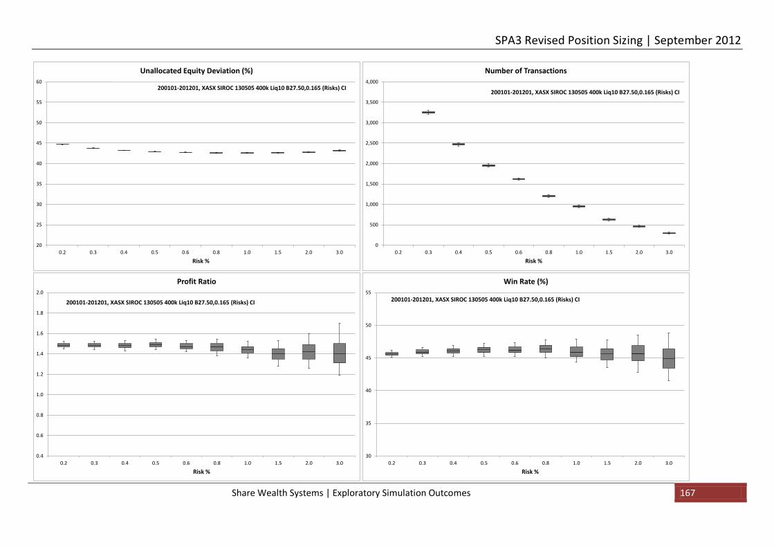
SPA3 Revised Position Sizing | September 2012
Share Wealth Systems | Exploratory Simulation Outcomes 167
20
25
30
35
40
45
50
55
60
0.2 0.3 0.4 0.5 0.6 0.8 1.0 1.5 2.0 3.0
Risk %
Unallocated Equity Deviation (%)
200101-201201, XASX SIROC 130505 400k Liq10 B27.50,0.165 (Risks) CI
0
500
1,000
1,500
2,000
2,500
3,000
3,500
4,000
0.2 0.3 0.4 0.5 0.6 0.8 1.0 1.5 2.0 3.0
Risk %
Number of Transactions
200101-201201, XASX SIROC 130505 400k Liq10 B27.50,0.165 (Risks) CI
0.4
0.6
0.8
1.0
1.2
1.4
1.6
1.8
2.0
0.2 0.3 0.4 0.5 0.6 0.8 1.0 1.5 2.0 3.0
Risk %
Profit Ratio
200101-201201, XASX SIROC 130505 400k Liq10 B27.50,0.165 (Risks) CI
30
35
40
45
50
55
0.2 0.3 0.4 0.5 0.6 0.8 1.0 1.5 2.0 3.0
Risk %
Win Rate (%)
200101-201201, XASX SIROC 130505 400k Liq10 B27.50,0.165 (Risks) CI

SPA3 Revised Position Sizing | September 2012
Share Wealth Systems | Exploratory Simulation Outcomes 168
11.4 Portfolio Simulated Equity Curves and Box Plots for SIROC 13 5 5 – Leave trades open
This section shows equity curves using the risk management tactic of leaving SPA3 trades open when the market turns to High Risk. SPA3 trades are only closed when an exit signal occurs for each individual trade after the High Risk signal has occurred. In some instances trades can remain open for weeks through the High Risk period.
One the biggest changes that the reader will notice in this section compared to the “Close immediately” section is the “Unallocated Equity” box plots show that capital is typically allocated about 10% more with the “Leave trades open” approach.
11.4.1 25k Charts: SIROC 130505, x10 Liquidity Check, $27.50 or 0.165% Brokerage
The six straw-broom charts have been simulated with the following Portfolio Risk % to calculate the position sizes, in order:
1. Run 483 0.5% Portfolio Risk %. 2. Run 486 0.6%. 3. Run 489 0.8% 4. Run 492 1.0% 5. Run 495 1.5% 6. Run 498 2% 7. Run 480 3%
None of these positions sizes would be good enough with which to trade. Note how poorly the smallest position size of 0.5% as the Portfolio Risk % did. This shows complete portfolio meltdown due to paying very high brokerage rates relative to tiny position sizes resulting from a small starting capital.
Just a small increase in position size to 0.6% shows the sensitivity of small portfolios to positions size. All with the same entry and exit signals in individual trades.
You should get the message from these simulations that trading with a small amount of capital has the odds greatly stacked against the active investor when paying a brokerage rate that is relatively too large for the amount of trading capital.

SPA3 Revised Position Sizing | September 2012
Share Wealth Systems | Exploratory Simulation Outcomes 169

SPA3 Revised Position Sizing | September 2012
Share Wealth Systems | Exploratory Simulation Outcomes 170
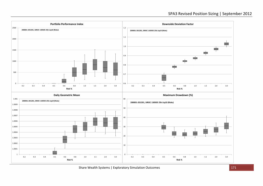
SPA3 Revised Position Sizing | September 2012
Share Wealth Systems | Exploratory Simulation Outcomes 171
0
500
1000
1500
2000
2500
0.2 0.3 0.4 0.5 0.6 0.8 1.0 1.5 2.0 3.0
Risk %
Portfolio Performance Index
200001-201201, SIROC 130505 25k Liq10 (Risks)
0.6
0.7
0.8
0.9
1.0
1.1
1.2
0.2 0.3 0.4 0.5 0.6 0.8 1.0 1.5 2.0 3.0
Risk %
Downside Deviation Factor
200001-201201, SIROC 130505 25k Liq10 (Risks)
1
1.0001
1.0002
1.0003
1.0004
1.0005
1.0006
1.0007
1.0008
1.0009
1.001
0.2 0.3 0.4 0.5 0.6 0.8 1.0 1.5 2.0 3.0
Risk %
Daily Geometric Mean
200001-201201, SIROC 130505 25k Liq10 (Risks)
0
10
20
30
40
50
60
0.2 0.3 0.4 0.5 0.6 0.8 1.0 1.5 2.0 3.0
Risk %
Maximum Drawdown (%)
200001-201201, SIROC 130505 25k Liq10 (Risks)

SPA3 Revised Position Sizing | September 2012
Share Wealth Systems | Exploratory Simulation Outcomes 172
30
31
32
33
34
35
36
37
38
39
40
0.2 0.3 0.4 0.5 0.6 0.8 1.0 1.5 2.0 3.0
Risk %
Unallocated Equity Deviation (%)
200001-201201, SIROC 130505 25k Liq10 (Risks)
0
500
1,000
1,500
2,000
2,500
3,000
3,500
4,000
4,500
5,000
0.2 0.3 0.4 0.5 0.6 0.8 1.0 1.5 2.0 3.0
Risk %
Number of Transactions
200001-201201, SIROC 130505 25k Liq10 (Risks)
0.6
0.8
1.0
1.2
1.4
1.6
1.8
0.2 0.3 0.4 0.5 0.6 0.8 1.0 1.5 2.0 3.0
Risk %
Profit Ratio
200001-201201, SIROC 130505 25k Liq10 (Risks)
35
40
45
50
55
0.2 0.3 0.4 0.5 0.6 0.8 1.0 1.5 2.0 3.0
Risk %
Win Rate (%)
200001-201201, SIROC 130505 25k Liq10 (Risks)

SPA3 Revised Position Sizing | September 2012
Share Wealth Systems | Exploratory Simulation Outcomes 173
11.4.2 25k Charts: SIROC 130505, x10 Liquidity Check, $19.95 or 0.1% Brokerage
The seven straw-broom charts have been simulated with the following Portfolio Risk % to calculate the position sizes, in order:
1. Run 481 0.4% Portfolio Risk %. 2. Run 484 0.5% 3. Run 487 0.6%. 4. Run 490 0.8% 5. Run 493 1.0% 6. Run 496 1.5% 7. Run 499 2%
Note what a big difference the drop in the minimum brokerage from $27.50 to $19.95 makes when trading with a small starting capital.
The 0.6% - 0.8% Portfolio Risk % would be viable but it is recommended to trade with lower brokerage levels for a small portfolio, or, at these brokerage levels to start with more capital of around $40,000.
It is important to understand that with a small portfolio value the majority of trades are charged the minimum brokerage rate of $19.95 until the portfolio gets larger enough to get to the 0.11% level. This is why small portfolios are so sensitive to the minimum brokerage rate.
These SIROC 13 5 5 results can be compared with the SIROC 21 8 results in section 11.2.3 starting on page 47.

SPA3 Revised Position Sizing | September 2012
Share Wealth Systems | Exploratory Simulation Outcomes 174

SPA3 Revised Position Sizing | September 2012
Share Wealth Systems | Exploratory Simulation Outcomes 175

SPA3 Revised Position Sizing | September 2012
Share Wealth Systems | Exploratory Simulation Outcomes 176
0
500
1000
1500
2000
2500
0.2 0.3 0.4 0.5 0.6 0.8 1.0 1.5 2.0 3.0
Risk %
Portfolio Performance Index
200101-201201, XASX SIROC 130505 25k Liq10 (Risks)
0.5
0.6
0.7
0.8
0.9
1.0
1.1
1.2
0.2 0.3 0.4 0.5 0.6 0.8 1.0 1.5 2.0 3.0
Risk %
Downside Deviation Factor
200101-201201, XASX SIROC 130505 25k Liq10 (Risks)
1
1.0001
1.0002
1.0003
1.0004
1.0005
1.0006
1.0007
1.0008
1.0009
1.001
0.2 0.3 0.4 0.5 0.6 0.8 1.0 1.5 2.0 3.0
Risk %
Daily Geometric Mean
200101-201201, XASX SIROC 130505 25k Liq10 (Risks)
0
10
20
30
40
50
60
0.2 0.3 0.4 0.5 0.6 0.8 1.0 1.5 2.0 3.0
Risk %
Maximum Drawdown (%)
200101-201201, XASX SIROC 130505 25k Liq10 (Risks)

SPA3 Revised Position Sizing | September 2012
Share Wealth Systems | Exploratory Simulation Outcomes 177
20
25
30
35
40
45
50
55
60
0.2 0.3 0.4 0.5 0.6 0.8 1.0 1.5 2.0 3.0
Risk %
Unallocated Equity Deviation (%)
200101-201201, XASX SIROC 130505 25k Liq10 (Risks)
0
500
1,000
1,500
2,000
2,500
3,000
3,500
4,000
0.2 0.3 0.4 0.5 0.6 0.8 1.0 1.5 2.0 3.0
Risk %
Number of Transactions
200101-201201, XASX SIROC 130505 25k Liq10 (Risks)
0.4
0.6
0.8
1.0
1.2
1.4
1.6
1.8
2.0
0.2 0.3 0.4 0.5 0.6 0.8 1.0 1.5 2.0 3.0
Risk %
Profit Ratio
200101-201201, XASX SIROC 130505 25k Liq10 (Risks)
30
35
40
45
50
55
0.2 0.3 0.4 0.5 0.6 0.8 1.0 1.5 2.0 3.0
Risk %
Win Rate (%)
200101-201201, XASX SIROC 130505 25k Liq10 (Risks)

SPA3 Revised Position Sizing | September 2012
Share Wealth Systems | Exploratory Simulation Outcomes 178
11.4.3 25k Charts: SIROC 130505, x10 Liquidity Check, $9.90 or 0.1% Brokerage
The ten straw-broom charts have been simulated with the following Portfolio Risk % to calculate the position sizes, in order:
1. Run 628 0.2% Portfolio Risk %. 2. Run 631 0.3%. 3. Run 634 0.4%. 4. Run 630 0.5%. 5. Run 633 0.6%. 6. Run 636 0.8%. 7. Run 639 1%. 8. Run 642 1.5%. 9. Run 645 2%. 10. Run 627 3%.
With the lower brokerage rates it is now viable to simulate smaller position sizes than the 0.5% in the previous section. Ensure that you compare like on like position sizes when comparing straw-broom equity curves from one portfolio scenario to another in other sections.
For small portfolio starting capital using a broker with a low minimum brokerage rate makes a huge difference to returns, drawdown and compounding of being able to use your money for re-investing rather than paying that money away in brokerage.
The portfolio meltdown caused purely by brokerage is largely removed when used a minimum brokerage rate as low as $9.90. Obviously using a minimum brokerage rate of $15 or 0.1%, or $16.50 or 0.11% can work with a small portfolio and would be far better than $19.95 but the lower that the minimum rate the better, especially with a small portfolio.
This set of simulations with SIROC 13 5 5 ‘leave trades open’ can be compared to the simulations with SIROC 13 5 5 ‘close immediately’ in section 11.3.4 on page 118. The major notable difference is that the ‘leave trades open’ fared much better during the second half of 2000 to early 2001 and during the first half of 2004 than the ‘close immediately’ approach. Neither is right or wrong. This research bears out that one will work better in certain market conditions and the other in other market conditions that will only become evident after the fact. In general, one might conclude that the ‘leave trades open’ will work better during secular bull market conditions.

SPA3 Revised Position Sizing | September 2012
Share Wealth Systems | Exploratory Simulation Outcomes 179

SPA3 Revised Position Sizing | September 2012
Share Wealth Systems | Exploratory Simulation Outcomes 180
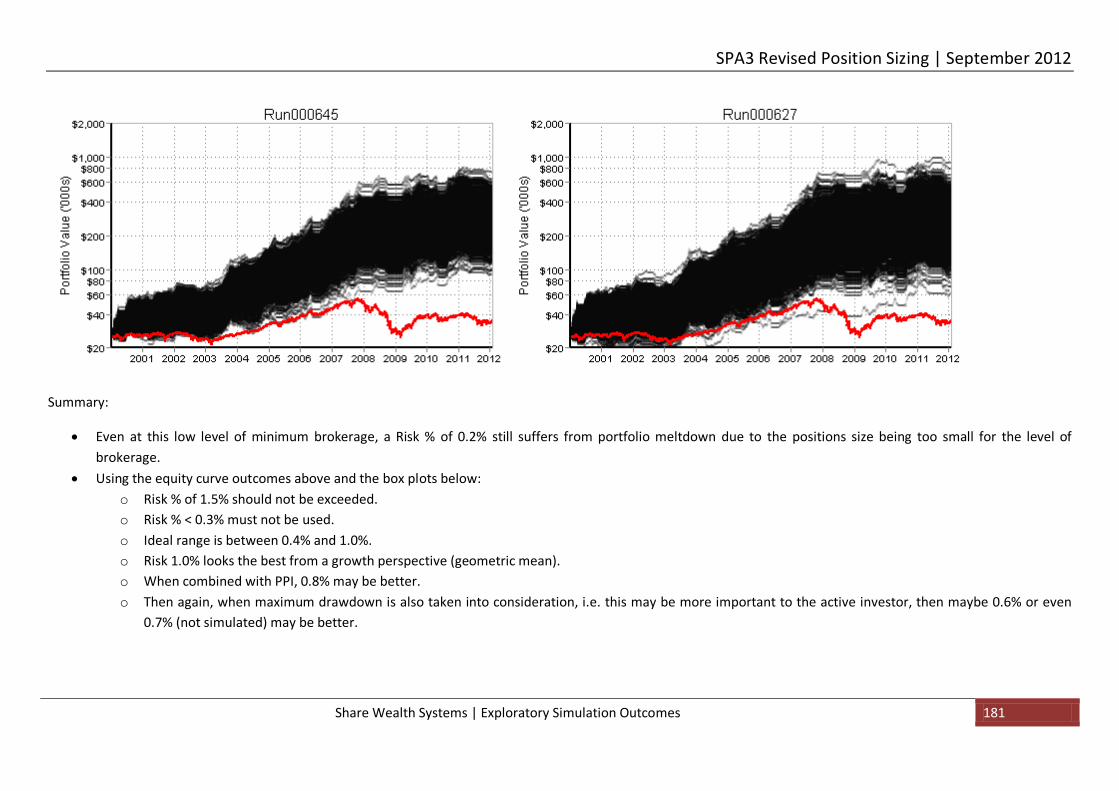
SPA3 Revised Position Sizing | September 2012
Share Wealth Systems | Exploratory Simulation Outcomes 181
Summary:
• Even at this low level of minimum brokerage, a Risk % of 0.2% still suffers from portfolio meltdown due to the positions size being too small for the level of brokerage.
• Using the equity curve outcomes above and the box plots below: o Risk % of 1.5% should not be exceeded. o Risk % < 0.3% must not be used. o Ideal range is between 0.4% and 1.0%. o Risk 1.0% looks the best from a growth perspective (geometric mean). o When combined with PPI, 0.8% may be better. o Then again, when maximum drawdown is also taken into consideration, i.e. this may be more important to the active investor, then maybe 0.6% or even
0.7% (not simulated) may be better.

SPA3 Revised Position Sizing | September 2012
Share Wealth Systems | Exploratory Simulation Outcomes 182
0
500
1000
1500
2000
2500
0.2 0.3 0.4 0.5 0.6 0.8 1.0 1.5 2.0 3.0
Risk %
Portfolio Performance Index
200101-201201, XASX SIROC 130505 25k Liq10 B9.90,0.1 (Risks)
0.5
0.6
0.7
0.8
0.9
1.0
1.1
1.2
0.2 0.3 0.4 0.5 0.6 0.8 1.0 1.5 2.0 3.0
Risk %
Downside Deviation Factor
200101-201201, XASX SIROC 130505 25k Liq10 B9.90,0.1 (Risks)
1
1.0001
1.0002
1.0003
1.0004
1.0005
1.0006
1.0007
1.0008
1.0009
1.001
0.2 0.3 0.4 0.5 0.6 0.8 1.0 1.5 2.0 3.0
Risk %
Daily Geometric Mean
200101-201201, XASX SIROC 130505 25k Liq10 B9.90,0.1 (Risks)
0
10
20
30
40
50
60
0.2 0.3 0.4 0.5 0.6 0.8 1.0 1.5 2.0 3.0
Risk %
Maximum Drawdown (%)
200101-201201, XASX SIROC 130505 25k Liq10 B9.90,0.1 (Risks)

SPA3 Revised Position Sizing | September 2012
Share Wealth Systems | Exploratory Simulation Outcomes 183
20
25
30
35
40
45
50
55
60
0.2 0.3 0.4 0.5 0.6 0.8 1.0 1.5 2.0 3.0
Risk %
Unallocated Equity Deviation (%)
200101-201201, XASX SIROC 130505 25k Liq10 B9.90,0.1 (Risks)
0
500
1,000
1,500
2,000
2,500
3,000
3,500
4,000
0.2 0.3 0.4 0.5 0.6 0.8 1.0 1.5 2.0 3.0
Risk %
Number of Transactions
200101-201201, XASX SIROC 130505 25k Liq10 B9.90,0.1 (Risks)
0.4
0.6
0.8
1.0
1.2
1.4
1.6
1.8
2.0
0.2 0.3 0.4 0.5 0.6 0.8 1.0 1.5 2.0 3.0
Risk %
Profit Ratio
200101-201201, XASX SIROC 130505 25k Liq10 B9.90,0.1 (Risks)
30
35
40
45
50
55
0.2 0.3 0.4 0.5 0.6 0.8 1.0 1.5 2.0 3.0
Risk %
Win Rate (%)
200101-201201, XASX SIROC 130505 25k Liq10 B9.90,0.1 (Risks)

SPA3 Revised Position Sizing | September 2012
Share Wealth Systems | Exploratory Simulation Outcomes 184
11.4.3.1 Individual Equity Curves & Underwater Equity Curves
Using the above graphical output, assume a Portfolio Risk % of 1.0%. From run 639 above we know that there were 1000 unique equity curves generated by selecting trades randomly when there was available capital, according to the SPA3 entry & exit criteria and the risk management & position sizing rules. We have selected a two individual portfolios from the 1000 portfolio simulation that may be representative of a potential equity curve outcome to assist positioning how a SPA3 trader’s equity curve may eventuate, provided that the rules are followed in a mechanical manner:
1. The median geometrical mean. This is the portfolio that ended at the 50th percentile, that is, middle line on the box plot. Half of the 1000 portfolios would have performed better and half worse at the end of the simulation period. This does not mean that it would have been the median portfolio all the way through the simulation period. This the first set of graphs.
2. The maximum drawdown at the 95th percentile. This is the portfolio that had 95% of portfolios with a better (lower or shallower) maximum drawdown and 5% that had worse maximum drawdowns. This the second set of graphs.
The following graphs are provided for each of the two equity curves:
1. The mark-to-market equity curve in arithmetic and then log mode. The red plot is the All Ordinaries Index. 2. The % drawdown underwater equity curve for the portfolio with the vertical axis scaled according to the maximum drawdown reached in the life of the portfolio. 3. The underwater curve for the portfolio (black shadow) compared to the underwater curve for the All Ordinaries Index (red shadow). 4. The open positions through the life of the portfolio. The periods where they are no open positions are when the portfolio was 100% in cash during High Market Risk
periods, according to Risk Profile 1.

SPA3 Revised Position Sizing | September 2012
Share Wealth Systems | Exploratory Simulation Outcomes 185
-60.00
-50.00
-40.00
-30.00
-20.00
-10.00
0.00
2000
0104
2000
0426
2000
0814
2000
1129
2001
0322
2001
0713
2001
1030
2002
0220
2002
0613
2002
0930
2003
0120
2003
0513
2003
0829
2003
1216
2004
0407
2004
0728
2004
1112
2005
0307
2005
0628
2005
1013
2006
0203
2006
0526
2006
0913
2007
0103
2007
0426
2007
0814
2007
1129
2008
0325
2008
0714
2008
1029
2009
0219
2009
0611
2009
0928
2010
0118
2010
0511
2010
0827
2010
1214
2011
0406
2011
0728
2011
1114
Underwater Equity Curve compared to the All Ordinaries

SPA3 Revised Position Sizing | September 2012
Share Wealth Systems | Exploratory Simulation Outcomes 186

SPA3 Revised Position Sizing | September 2012
Share Wealth Systems | Exploratory Simulation Outcomes 187

SPA3 Revised Position Sizing | September 2012
Share Wealth Systems | Exploratory Simulation Outcomes 188
11.4.4 100k Charts: SIROC 130505, x5 Liquidity Check, $27.50 or 0.165% Brokerage
1. Run 731 0.2% Portfolio Risk %. 2. Run 732 0.3%. 3. Run 733 0.4%. 4. Run 734 0.5%. 5. Run 735 0.6%. 6. Run 736 0.8%. 7. Run 737 1%. 8. Run 738 1.5%. 9. Run 739 2%.

SPA3 Revised Position Sizing | September 2012
Share Wealth Systems | Exploratory Simulation Outcomes 189
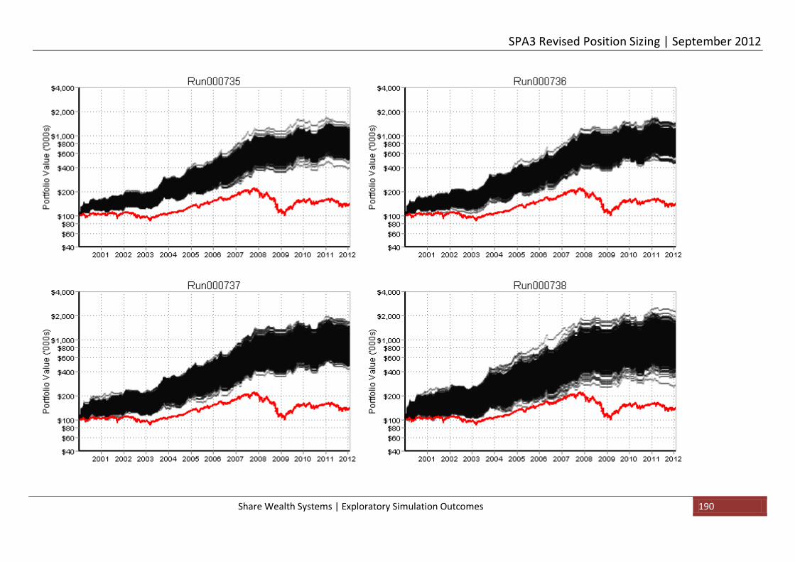
SPA3 Revised Position Sizing | September 2012
Share Wealth Systems | Exploratory Simulation Outcomes 190

SPA3 Revised Position Sizing | September 2012
Share Wealth Systems | Exploratory Simulation Outcomes 191
Summary:
• Even at this low level of minimum brokerage, a Risk % of 0.2% still suffers from portfolio meltdown due to the positions size being too small for the level of brokerage.
• Using the equity curve outcomes above and the box plots below: o Risk % of 1.5% should not be exceeded. o Risk % < 0.3% must not be used. o Ideal range is between 0.4% and 1.0%. o Risk 1.0% looks the best from a growth perspective (geometric mean). o When combined with PPI, 0.8% may be better. o Then again, when maximum drawdown is also taken into consideration, i.e. this may be more important to the active investor, then maybe 0.6% or even
0.7% (not simulated) may be better.

SPA3 Revised Position Sizing | September 2012
Share Wealth Systems | Exploratory Simulation Outcomes 192
0
500
1000
1500
2000
2500
0.2 0.3 0.4 0.5 0.6 0.8 1.0 1.5 2.0 3.0
Risk %
Portfolio Performance Index
200101-201201, XASX SIROC 130505 100k Liq05 (Risks)
0.5
0.6
0.7
0.8
0.9
1.0
1.1
1.2
0.2 0.3 0.4 0.5 0.6 0.8 1.0 1.5 2.0 3.0
Risk %
Downside Deviation Factor
200101-201201, XASX SIROC 130505 100k Liq05 (Risks)
1
1.0001
1.0002
1.0003
1.0004
1.0005
1.0006
1.0007
1.0008
1.0009
1.001
0.2 0.3 0.4 0.5 0.6 0.8 1.0 1.5 2.0 3.0
Risk %
Daily Geometric Mean
200101-201201, XASX SIROC 130505 100k Liq05 (Risks)
0
10
20
30
40
50
60
0.2 0.3 0.4 0.5 0.6 0.8 1.0 1.5 2.0 3.0
Risk %
Maximum Drawdown (%)
200101-201201, XASX SIROC 130505 100k Liq05 (Risks)

SPA3 Revised Position Sizing | September 2012
Share Wealth Systems | Exploratory Simulation Outcomes 193
20
25
30
35
40
45
50
55
60
0.2 0.3 0.4 0.5 0.6 0.8 1.0 1.5 2.0 3.0
Risk %
Unallocated Equity Deviation (%)
200101-201201, XASX SIROC 130505 100k Liq05 (Risks)
0
500
1,000
1,500
2,000
2,500
3,000
3,500
4,000
0.2 0.3 0.4 0.5 0.6 0.8 1.0 1.5 2.0 3.0
Risk %
Number of Transactions
200101-201201, XASX SIROC 130505 100k Liq05 (Risks)
0.4
0.6
0.8
1.0
1.2
1.4
1.6
1.8
2.0
0.2 0.3 0.4 0.5 0.6 0.8 1.0 1.5 2.0 3.0
Risk %
Profit Ratio
200101-201201, XASX SIROC 130505 100k Liq05 (Risks)
30
35
40
45
50
55
0.2 0.3 0.4 0.5 0.6 0.8 1.0 1.5 2.0 3.0
Risk %
Win Rate (%)
200101-201201, XASX SIROC 130505 100k Liq05 (Risks)

SPA3 Revised Position Sizing | September 2012
Share Wealth Systems | Exploratory Simulation Outcomes 194
11.4.5 100k Charts: SIROC 130505, x10 Liquidity Check, $27.50 or 0.165% Brokerage
1. Run 611 0.2% Portfolio Risk %. 2. Run 613 0.3% 3. Run 459 0.4% 4. Run 462 0.5%. 5. Run 465 0.6%. 6. Run 468 0.8%. 7. Run 471 1%. 8. Run 474 1.5%. 9. Run 477 2%.

SPA3 Revised Position Sizing | September 2012
Share Wealth Systems | Exploratory Simulation Outcomes 195

SPA3 Revised Position Sizing | September 2012
Share Wealth Systems | Exploratory Simulation Outcomes 196

SPA3 Revised Position Sizing | September 2012
Share Wealth Systems | Exploratory Simulation Outcomes 197

SPA3 Revised Position Sizing | September 2012
Share Wealth Systems | Exploratory Simulation Outcomes 198
0
500
1000
1500
2000
2500
0.2 0.3 0.4 0.5 0.6 0.8 1.0 1.5 2.0 3.0
Risk %
Portfolio Performance Index
200101-201201, XASX SIROC 130505 100k Liq10 (Risks)
0.5
0.6
0.7
0.8
0.9
1.0
1.1
1.2
0.2 0.3 0.4 0.5 0.6 0.8 1.0 1.5 2.0 3.0
Risk %
Downside Deviation Factor
200101-201201, XASX SIROC 130505 100k Liq10 (Risks)
1
1.0001
1.0002
1.0003
1.0004
1.0005
1.0006
1.0007
1.0008
1.0009
1.001
0.2 0.3 0.4 0.5 0.6 0.8 1.0 1.5 2.0 3.0
Risk %
Daily Geometric Mean
200101-201201, XASX SIROC 130505 100k Liq10 (Risks)
0
10
20
30
40
50
60
0.2 0.3 0.4 0.5 0.6 0.8 1.0 1.5 2.0 3.0
Risk %
Maximum Drawdown (%)
200101-201201, XASX SIROC 130505 100k Liq10 (Risks)

SPA3 Revised Position Sizing | September 2012
Share Wealth Systems | Exploratory Simulation Outcomes 199
20
25
30
35
40
45
50
55
60
0.2 0.3 0.4 0.5 0.6 0.8 1.0 1.5 2.0 3.0
Risk %
Unallocated Equity Deviation (%)
200101-201201, XASX SIROC 130505 100k Liq10 (Risks)
0
500
1,000
1,500
2,000
2,500
3,000
3,500
4,000
0.2 0.3 0.4 0.5 0.6 0.8 1.0 1.5 2.0 3.0
Risk %
Number of Transactions
200101-201201, XASX SIROC 130505 100k Liq10 (Risks)
0.4
0.6
0.8
1.0
1.2
1.4
1.6
1.8
2.0
0.2 0.3 0.4 0.5 0.6 0.8 1.0 1.5 2.0 3.0
Risk %
Profit Ratio
200101-201201, XASX SIROC 130505 100k Liq10 (Risks)
30
35
40
45
50
55
0.2 0.3 0.4 0.5 0.6 0.8 1.0 1.5 2.0 3.0
Risk %
Win Rate (%)
200101-201201, XASX SIROC 130505 100k Liq10 (Risks)

SPA3 Revised Position Sizing | September 2012
Share Wealth Systems | Exploratory Simulation Outcomes 200
11.4.6 100k Charts: SIROC 130505, x5 Liquidity Check, $9.90 or 0.1% Brokerage
1. Run 605 0.2% Portfolio Risk %. 2. Run 608 0.3% 3. Run 460 0.4% 4. Run 463 0.5%. 5. Run 466 0.6%. 6. Run 469 0.8%. 7. Run 472 1%. 8. Run 475 1.5%. 9. Run 478 2%.

SPA3 Revised Position Sizing | September 2012
Share Wealth Systems | Exploratory Simulation Outcomes 201

SPA3 Revised Position Sizing | September 2012
Share Wealth Systems | Exploratory Simulation Outcomes 202

SPA3 Revised Position Sizing | September 2012
Share Wealth Systems | Exploratory Simulation Outcomes 203
Summary:
• The drop in brokerage has greatly improved the performance as seen quite notably on the PPI and Geometric Mean box plots below compared to the previous simulation with $27.50 / 0.165%.

SPA3 Revised Position Sizing | September 2012
Share Wealth Systems | Exploratory Simulation Outcomes 204
0
500
1000
1500
2000
2500
0.2 0.3 0.4 0.5 0.6 0.8 1.0 1.5 2.0 3.0
Risk %
Portfolio Performance Index
200101-201201, XASX SIROC 130505 100k Liq05 B9.90,0.1 (Risks)
0.5
0.6
0.7
0.8
0.9
1.0
1.1
1.2
0.2 0.3 0.4 0.5 0.6 0.8 1.0 1.5 2.0 3.0
Risk %
Downside Deviation Factor
200101-201201, XASX SIROC 130505 100k Liq05 B9.90,0.1 (Risks)
1
1.0001
1.0002
1.0003
1.0004
1.0005
1.0006
1.0007
1.0008
1.0009
1.001
0.2 0.3 0.4 0.5 0.6 0.8 1.0 1.5 2.0 3.0
Risk %
Daily Geometric Mean
200101-201201, XASX SIROC 130505 100k Liq05 B9.90,0.1 (Risks)
0
10
20
30
40
50
60
0.2 0.3 0.4 0.5 0.6 0.8 1.0 1.5 2.0 3.0
Risk %
Maximum Drawdown (%)
200101-201201, XASX SIROC 130505 100k Liq05 B9.90,0.1 (Risks)

SPA3 Revised Position Sizing | September 2012
Share Wealth Systems | Exploratory Simulation Outcomes 205
20
25
30
35
40
45
50
55
60
0.2 0.3 0.4 0.5 0.6 0.8 1.0 1.5 2.0 3.0
Risk %
Unallocated Equity Deviation (%)
200101-201201, XASX SIROC 130505 100k Liq05 B9.90,0.1 (Risks)
0
500
1,000
1,500
2,000
2,500
3,000
3,500
4,000
0.2 0.3 0.4 0.5 0.6 0.8 1.0 1.5 2.0 3.0
Risk %
Number of Transactions
200101-201201, XASX SIROC 130505 100k Liq05 B9.90,0.1 (Risks)
0.4
0.6
0.8
1.0
1.2
1.4
1.6
1.8
2.0
0.2 0.3 0.4 0.5 0.6 0.8 1.0 1.5 2.0 3.0
Risk %
Profit Ratio
200101-201201, XASX SIROC 130505 100k Liq05 B9.90,0.1 (Risks)
30
35
40
45
50
55
0.2 0.3 0.4 0.5 0.6 0.8 1.0 1.5 2.0 3.0
Risk %
Win Rate (%)
200101-201201, XASX SIROC 130505 100k Liq05 B9.90,0.1 (Risks)

SPA3 Revised Position Sizing | September 2012
Share Wealth Systems | Exploratory Simulation Outcomes 206
11.4.7 100k Charts: SIROC 130505, x10 Liquidity Check, $9.90 or 0.1% Brokerage
1. Run 607 0.2% Portfolio Risk %. 2. Run 610 0.3% 3. Run 606 0.4% 4. Run 609 0.5%. 5. Run 612 0.6%. 6. Run 615 0.8%. 7. Run 618 1%. 8. Run 621 1.5%. 9. Run 624 2%.

SPA3 Revised Position Sizing | September 2012
Share Wealth Systems | Exploratory Simulation Outcomes 207

SPA3 Revised Position Sizing | September 2012
Share Wealth Systems | Exploratory Simulation Outcomes 208

SPA3 Revised Position Sizing | September 2012
Share Wealth Systems | Exploratory Simulation Outcomes 209

SPA3 Revised Position Sizing | September 2012
Share Wealth Systems | Exploratory Simulation Outcomes 210
0
500
1000
1500
2000
2500
0.2 0.3 0.4 0.5 0.6 0.8 1.0 1.5 2.0 3.0
Risk %
Portfolio Performance Index
200101-201201, XASX SIROC 130505 100k Liq10 B9.90,0.1 (Risks)
0.5
0.6
0.7
0.8
0.9
1.0
1.1
1.2
0.2 0.3 0.4 0.5 0.6 0.8 1.0 1.5 2.0 3.0
Risk %
Downside Deviation Factor
200101-201201, XASX SIROC 130505 100k Liq10 B9.90,0.1 (Risks)
1
1.0001
1.0002
1.0003
1.0004
1.0005
1.0006
1.0007
1.0008
1.0009
1.001
0.2 0.3 0.4 0.5 0.6 0.8 1.0 1.5 2.0 3.0
Risk %
Daily Geometric Mean
200101-201201, XASX SIROC 130505 100k Liq10 B9.90,0.1 (Risks)
0
10
20
30
40
50
60
0.2 0.3 0.4 0.5 0.6 0.8 1.0 1.5 2.0 3.0
Risk %
Maximum Drawdown (%)
200101-201201, XASX SIROC 130505 100k Liq10 B9.90,0.1 (Risks)

SPA3 Revised Position Sizing | September 2012
Share Wealth Systems | Exploratory Simulation Outcomes 211
20
25
30
35
40
45
50
55
60
0.2 0.3 0.4 0.5 0.6 0.8 1.0 1.5 2.0 3.0
Risk %
Unallocated Equity Deviation (%)
200101-201201, XASX SIROC 130505 100k Liq10 B9.90,0.1 (Risks)
0
500
1,000
1,500
2,000
2,500
3,000
3,500
4,000
0.2 0.3 0.4 0.5 0.6 0.8 1.0 1.5 2.0 3.0
Risk %
Number of Transactions
200101-201201, XASX SIROC 130505 100k Liq10 B9.90,0.1 (Risks)
0.4
0.6
0.8
1.0
1.2
1.4
1.6
1.8
2.0
0.2 0.3 0.4 0.5 0.6 0.8 1.0 1.5 2.0 3.0
Risk %
Profit Ratio
200101-201201, XASX SIROC 130505 100k Liq10 B9.90,0.1 (Risks)
30
35
40
45
50
55
0.2 0.3 0.4 0.5 0.6 0.8 1.0 1.5 2.0 3.0
Risk %
Win Rate (%)
200101-201201, XASX SIROC 130505 100k Liq10 B9.90,0.1 (Risks)

SPA3 Revised Position Sizing | September 2012
Share Wealth Systems | Exploratory Simulation Outcomes 212
11.4.8 400k Charts: SIROC 130505, x5 Liquidity Check, $27.50 or 0.165% Brokerage
1. Run 653 0.2% Portfolio Risk %. 2. Run 655 0.3% 3. Run 502 0.4% 4. Run 505 0.5%. 5. Run 508 0.6%. 6. Run 511 0.8%. 7. Run 514 1%. 8. Run 517 1.5%. 9. Run 520 2%.

SPA3 Revised Position Sizing | September 2012
Share Wealth Systems | Exploratory Simulation Outcomes 213

SPA3 Revised Position Sizing | September 2012
Share Wealth Systems | Exploratory Simulation Outcomes 214
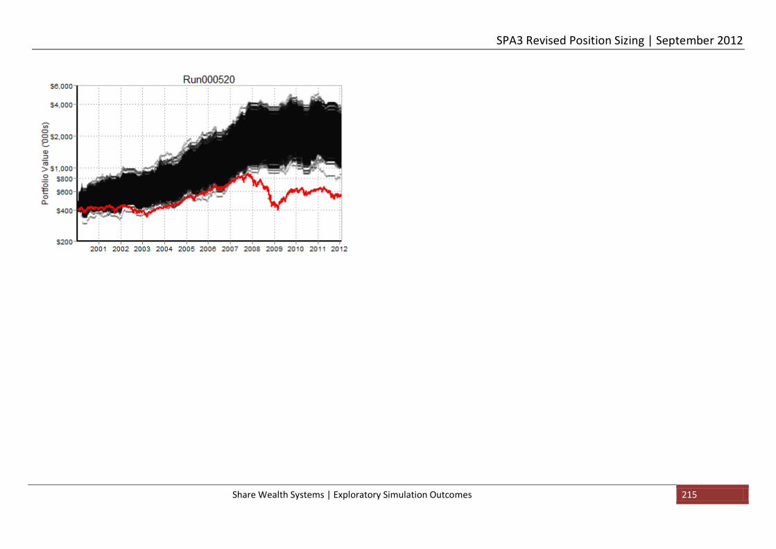
SPA3 Revised Position Sizing | September 2012
Share Wealth Systems | Exploratory Simulation Outcomes 215

SPA3 Revised Position Sizing | September 2012
Share Wealth Systems | Exploratory Simulation Outcomes 216
0
500
1000
1500
2000
2500
0.2 0.3 0.4 0.5 0.6 0.8 1.0 1.5 2.0 3.0
Risk %
Portfolio Performance Index
200101-201201, XASX SIROC 130505 400k Liq05 (Risks)
0.5
0.6
0.7
0.8
0.9
1.0
1.1
1.2
0.2 0.3 0.4 0.5 0.6 0.8 1.0 1.5 2.0 3.0
Risk %
Downside Deviation Factor
200101-201201, XASX SIROC 130505 400k Liq05 (Risks)
1
1.0001
1.0002
1.0003
1.0004
1.0005
1.0006
1.0007
1.0008
1.0009
1.001
0.2 0.3 0.4 0.5 0.6 0.8 1.0 1.5 2.0 3.0
Risk %
Daily Geometric Mean
200101-201201, XASX SIROC 130505 400k Liq05 (Risks)
0
10
20
30
40
50
60
0.2 0.3 0.4 0.5 0.6 0.8 1.0 1.5 2.0 3.0
Risk %
Maximum Drawdown (%)
200101-201201, XASX SIROC 130505 400k Liq05 (Risks)
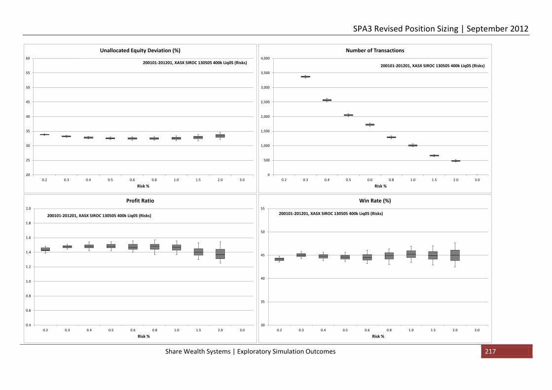
SPA3 Revised Position Sizing | September 2012
Share Wealth Systems | Exploratory Simulation Outcomes 217
20
25
30
35
40
45
50
55
60
0.2 0.3 0.4 0.5 0.6 0.8 1.0 1.5 2.0 3.0
Risk %
Unallocated Equity Deviation (%)
200101-201201, XASX SIROC 130505 400k Liq05 (Risks)
0
500
1,000
1,500
2,000
2,500
3,000
3,500
4,000
0.2 0.3 0.4 0.5 0.6 0.8 1.0 1.5 2.0 3.0
Risk %
Number of Transactions
200101-201201, XASX SIROC 130505 400k Liq05 (Risks)
0.4
0.6
0.8
1.0
1.2
1.4
1.6
1.8
2.0
0.2 0.3 0.4 0.5 0.6 0.8 1.0 1.5 2.0 3.0
Risk %
Profit Ratio
200101-201201, XASX SIROC 130505 400k Liq05 (Risks)
30
35
40
45
50
55
0.2 0.3 0.4 0.5 0.6 0.8 1.0 1.5 2.0 3.0
Risk %
Win Rate (%)
200101-201201, XASX SIROC 130505 400k Liq05 (Risks)

SPA3 Revised Position Sizing | September 2012
Share Wealth Systems | Exploratory Simulation Outcomes 218
11.4.9 400k Charts: SIROC 130505, x10 Liquidity Check, $27.50 or 0.165% Brokerage
1. Run 656 0.2% Portfolio Risk %. 2. Run 658 0.3% 3. Run 501 0.4% 4. Run 504 0.5%. 5. Run 507 0.6%. 6. Run 510 0.8%. 7. Run 513 1%. 8. Run 516 1.5%. 9. Run 519 2%.

SPA3 Revised Position Sizing | September 2012
Share Wealth Systems | Exploratory Simulation Outcomes 219

SPA3 Revised Position Sizing | September 2012
Share Wealth Systems | Exploratory Simulation Outcomes 220
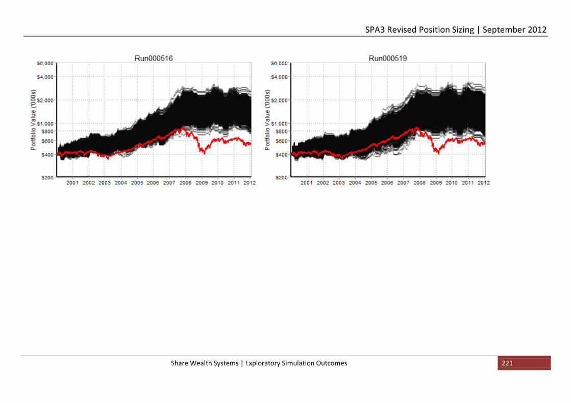
SPA3 Revised Position Sizing | September 2012
Share Wealth Systems | Exploratory Simulation Outcomes 221

SPA3 Revised Position Sizing | September 2012
Share Wealth Systems | Exploratory Simulation Outcomes 222
0
500
1000
1500
2000
2500
0.2 0.3 0.4 0.5 0.6 0.8 1.0 1.5 2.0 3.0
Risk %
Portfolio Performance Index
200101-201201, XASX SIROC 130505 400k Liq10 (Risks)
0.5
0.6
0.7
0.8
0.9
1.0
1.1
1.2
0.2 0.3 0.4 0.5 0.6 0.8 1.0 1.5 2.0 3.0
Risk %
Downside Deviation Factor
200101-201201, XASX SIROC 130505 400k Liq10 (Risks)
1
1.0001
1.0002
1.0003
1.0004
1.0005
1.0006
1.0007
1.0008
1.0009
1.001
0.2 0.3 0.4 0.5 0.6 0.8 1.0 1.5 2.0 3.0
Risk %
Daily Geometric Mean
200101-201201, XASX SIROC 130505 400k Liq10 (Risks)
0
10
20
30
40
50
60
0.2 0.3 0.4 0.5 0.6 0.8 1.0 1.5 2.0 3.0
Risk %
Maximum Drawdown (%)
200101-201201, XASX SIROC 130505 400k Liq10 (Risks)

SPA3 Revised Position Sizing | September 2012
Share Wealth Systems | Exploratory Simulation Outcomes 223
20
25
30
35
40
45
50
55
60
0.2 0.3 0.4 0.5 0.6 0.8 1.0 1.5 2.0 3.0
Risk %
Unallocated Equity Deviation (%)
200101-201201, XASX SIROC 130505 400k Liq10 (Risks)
0
500
1,000
1,500
2,000
2,500
3,000
3,500
4,000
0.2 0.3 0.4 0.5 0.6 0.8 1.0 1.5 2.0 3.0
Risk %
Number of Transactions
200101-201201, XASX SIROC 130505 400k Liq10 (Risks)
0.4
0.6
0.8
1.0
1.2
1.4
1.6
1.8
2.0
0.2 0.3 0.4 0.5 0.6 0.8 1.0 1.5 2.0 3.0
Risk %
Profit Ratio
200101-201201, XASX SIROC 130505 400k Liq10 (Risks)
30
35
40
45
50
55
0.2 0.3 0.4 0.5 0.6 0.8 1.0 1.5 2.0 3.0
Risk %
Win Rate (%)
200101-201201, XASX SIROC 130505 400k Liq10 (Risks)

SPA3 Revised Position Sizing | September 2012
Share Wealth Systems | Exploratory Simulation Summary
12 Exploratory Simulation Summary As is obvious from the above research, exploratory simulation allows detailed research and stress testing of risk and money management rules, especially during market periods that are atypical. As important as it is to research an edge, exploratory simulation is far more important as it helps determine the risk management rules that will protect capital, i.e. survive, and the associated money management rules that will help grow capital, i.e. thrive.
Undoubtedly the exploratory simulation conducted in this project has taken the SPA3 methodology to a new level. It is our considered view that the level of detailed inner workings provided for the SPA3 trading methodology is unprecedented. We are not aware of any educator that has researched a trading methodology to this level and then made all the information available to their customers, totally transparently.
We suggest that, over time, all the exploratory simulation information provided in this White Paper be studied. The educational value for trading in general is enormous.
Some ‘big picture’ conclusions from the exploratory simulation in this paper:
1. The SIROC 13 5 5 simulations with shorter and more sensitive market risk timing and stock timing demonstrated better performance than the SIROC 21 8 over the sample period. There were seven more Low Risk market cycles with the SIROC 13 5 5 than the SIROC 21 8. Considering that the sample research period covered a secular bear market period better performance may not be the case during a secular bull market sample period.
2. The major notable difference is that the ‘leave trades open’ fared much better during the second half of 2000 to early 2001 and during the first half of 2004 than the ‘close immediately’ approach. Neither is right or wrong. This research bears out that one will work better in certain market conditions and the other in other market conditions that will only become evident after the fact. In general, one might conclude that the ‘leave trades open’ will work better during secular bull market conditions.
3. “Unallocated Equity” box plots show that capital is typically allocated about 10% more with the “Leave trades open” approach than the “Close immediately” approach.
4. All the SIROC settings of 21 8, 19 7, 17 7 and 13 5 have demonstrated superior performance compared to the overall market benchmark, the All Ordinaries Index. With the SQN and Expectancy of the SIROC 19 7 and SIROC 17 7 being slightly better than the SIROC 21 8 and SIROC 13 5, it can be extrapolated that the exploratory simulation of the 19 7 and 17 7 settings will be as good, if not better, than the portfolio simulations shown in this paper.
5. The many variables that act on a portfolio. Traders need to be aware what the major variables are, how they affect their portfolio and how to counteract the negative variables.
6. Brokerage is one of the major variables that active investors need to be aware of and how to avoid portfolio meltdown.
7. Bigger position size doesn’t necessarily mean bigger performance. There is a point where the geometric mean, i.e. growth potential, starts falling. For example, larger positions require more liquidity which may not exist in the chosen market, therefore causing opportunity loss.
8. The portfolio simulations show that most maximum drawdowns occurred since October 2009. This is due to whipsawing. This period has proved to be one of the most difficult periods for active investing in any time frame, short medium or long, and in either direction, short and long.

SPA3 Revised Position Sizing | September 2012
Share Wealth Systems | White Paper Summary
13 White Paper Summary There are variables identified in this paper that interact on our portfolios that we can control. However, there are two other variables, amongst many others, that we cannot control, overall market performance and randomness of individual trade outcomes. These two variables and all the variables discussed in this paper can be controlled by avoiding them altogether, by being a market spectator.
However, this would remove us from the opportunity flow to grow our capital. And we have to grow our wealth in some fashion to overcome inflation which erodes the value of our wealth. Once in the game of investing, randomness plays a major role, especially in trade selections from day to day, or year to year for buy and holders. Our task is to narrow down the effect of this randomness on our outcomes.
We do this through:
• Subscribing to an active methodology that can remove market (systematic) risk altogether during certain market periods.
• Defining strict criteria within which to time and select trades. • Effective risk management, and • Effective money management.
If there was little or no randomness in trade selection, then the variation of portfolio equity curve outcomes would be very narrow or non-existent. One of the major strengths of exploratory simulation is that takes into account this randomness of trade selection. The determination of position size through countless iterations of exploratory simulation allows research to tell us, with the benefit of hindsight, how to minimise the effect of this randomness.
But even once we have the four points highlighted above in place, belief and trust in one’s chosen process is mandatory so that we don’t self sabotage ourselves by operating outside of the parameters that the research has delivered to us. This is where trading psychology comes in.
The information provided in this White Paper should instil confidence into users of the SPA3 methodology and inspire them to:
• trade the methodology according to the revised risk management and money management rules, • continue to trust the methodology even when it goes into drawdown, • minimise or preferably eliminate trading errors and mistakes.
The trading period since October 2009 has proved to be one of the most difficult periods for active investing in any time frame, short medium or long and in either direction, long or short. Portfolios of all types have struggled during this period either going nowhere or into drawdown, due to market whipsawing resulting from lack of business and economic confidence the world over.
This is when trust is tested – it’s not tested during bull markets. If active investors become market spectators it can only mean that either:
1. They believe (or must know in advance) that there will never be another secular bull market, or even another primary bull market within a secular bear market. This is obviously a big call. How can anybody know this – well they can’t. This is when you hear the cries of “But this time it’s different! We are in a new era.” Due to any number of reasons, such as HFT, technology changes , terrorism etc etc.
2. They have lost trust in their methodology and no longer believe that it can work for them.

SPA3 Revised Position Sizing | September 2012
Share Wealth Systems | White Paper Summary
3. They have lost trust in themselves being able to execute in the environment of the market.
Whichever it is, the kind of detailed research provided in this White Paper can only assist in helping investors regain their confidence and trust in the markets, the methodology and their ability to execute to grow their capital bases using the environment of the equity markets to do so.
Spectators don’t lose but neither do they learn or grow much either and they never get lucky. Sure, players can lose and get unlucky too but we only grow personally when we engage the game and we only grow our capital when we confront and overcome the risks and fears of the environment in which we play.
One of the major fears is drawdown. Given that drawdown is a dead certainty, how do private investors that wish to do it themselves continue to outperform the market whilst not allowing drawdown to get out of hand? By smart risk and money management rules, customised according to their own requirements.
One of the other main changes in the SWS approach with SPA3 that has been highlighted since the December 2011 White Paper is that:
1. The individual trader’s Risk Objective has to be decided upon in the Objectives Statement of the Trading Plan.
2. Then Risk and Money Management rules need to be customised specifically according to the user’s Reward and Risk Objectives. What a particular user sets as their risk criteria to determine when to trade and not to trade and what position size to trade with will be done according to exploratory simulation.
Adjusting your position size according to one’s risk criteria, which is turn is set based on the Trading Plan Risk Objective, has become a key ingredient of SPA3.
For example, assume that a SPA3 user has a Risk Objective of 15%, i.e. will tolerate a maximum drawdown of 15%, then a position size should be selected from the information in this White Paper that has a maximum drawdown as close as possible to this Risk Objective, recognising that all other drawdowns would have been under the maximum drawdown. If the Risk Objective is reached it may be assumed that extreme negative market conditions have occurred at which time the SPA3 user can cease trading until a new Low Risk Market begins again.
As has been stated, Risk & Money Management will be the biggest determinant of portfolio outcomes regardless of how good an edge is. This is the important role that exploratory simulation has played is assisting an active investor survive in tough times and thrive in good times.
Lastly, we anticipate much discussion and questions about this paper. The SPA3 Forum will be the best place for such discussion.

SPA3 Revised Position Sizing | September 2012
Share Wealth Systems | Acknowledgements
14 Acknowledgements David Sayer.
David has been involved across the whole research process but more specifically in the exploratory simulation using complex portfolio simulation software and ‘R’ statistical programming to generate straw-broom graphical outputs and individual portfolio equity curves.
The portfolio simulation software used is flexible in the extreme but with flexibility comes complexity requiring low level programming in C++. Such research is massively detailed and time consuming and requires enormous attention to detail.
It also requires establishing processes and building peripheral tools in Excel and elsewhere to be able to conduct and keep track of the simulations and record them in an orderly manner for retrieval and analysis. David was dedicated for over a year on this one research project. There is still more to do …….
This project has touched the whole Share Wealth Systems team to some degree or another, some more than others. All have either put in a great effort or have put up with those that have had their heads stuck deep in research mode.
Paper written by Gary Stone.
15 References There are many many books that can be referenced. At the risk of devaluing a key book that has assisted greatly in this particular research project by just including it in a list, I have singled it out:
Trading Systems That Work, Thomas Stridsman, McGraw Hill, 2000
Other references in order of importance:
"Finance and Monte Carlo Simulation," Journal of Financial Planning, Nov. 2001 by David Nawrocki, Ph.D.
Van Tharp’s Definitive Guide to Position Sizing, 2008

SPA3 Revised Position Sizing | September 2012
Share Wealth Systems | Appendix A - Single Profit Stop
16 Appendix A - Single Profit Stop With the release of the SPA3 Revised Position Sizing the Profit Stop has been modified to only provide a single Profit Stop signal whenever consecutive SPA3 entry signals occur before an exit signal occurs. In the prior release a Profit Stop signal occurred for every entry signal. In the example below the first Profit Stop was ‘linked’ to the first SPA3 entry signal, a WCB4. Price action rolled over before a Profit Stop was reached for the second SPA3 signal. A WONS1+DS exit occurred for the second SPA3 entry signal.
The modification to a single Profit Stop only applies when more than one SPA3 entry signal occurs without an exit signal occurring in between. Typically the first entry signal will be a WCB4 following by a WONB4+DB or WCB1+RSC+DB, or a WCB3 followed by another WCB3.
When multiple consecutive entry signals occur SPA3 applies some simple logic whereby the Profit Stop for the first entry signal is increased and the Profit Stop for the second is marginally decreased. If the Profit Stop is reached then this becomes the Profit Stop for both entry signals. In the case of TOX below the Profit Stop is not reached so both entries are exited on the WONS1+DS.

SPA3 Revised Position Sizing | September 2012
Share Wealth Systems | Appendix A - Single Profit Stop
For a sequence of Buy signals there shall be only one profit stop value, known as the Profit Stop. Interim values calculated at different times for different signal may not be the Profit Stop for that bar. All profit stops are calculated from the most current Buy signals close price.
First Buy signal
The first Buy shall calculate a profit stop using the formula:
• signal profit stop = Signal Price x (1 + ATRVE_PS%) Where ATRVE_PS% is the profit stop percentage specified by the ATRVE value.
The Profit Stop is set to this initial signal profit stop until otherwise altered by another Buy signal.
Subsequent Buy signals
Subsequent Buy signals shall alter the Profit Stop according to these rules:
If the current signal price is less than or equal to the last signal price:
• signal profit stop = Signal Price x (1 + ATRVE_PS%)
The Profit Stop shall be set to the greater of the signal profit stop or the current Profit Stop value.

SPA3 Revised Position Sizing | September 2012
Share Wealth Systems | Appendix A - Single Profit Stop
If the current signal price is greater than the last signal price:
• signal profit stop = Signal Price x (1 + ATRVE_PS% x FACTOR) Where FACTOR = 1 - [ (‘The number of times the Profit Stop has been increased’ + 1) x 0.25 ]
The Profit Stop shall be set to the greater of the signal profit stop or the current Profit Stop value.
Other scenarios:
• If a Buy signal and a Profit Stop exit signal occur on the same day, ‘the Profit Stop’ shall be extended by calculating a value as per the above rules but the Buy signal shall not be displayed.
• If the SPA3 logic enters a WONS1 state, the Profit Stop is suspended. • A DB pyramid signal does not alter the Profit Stop.

SPA3 Revised Position Sizing | September 2012
Share Wealth Systems | Appendix B - Volatility Drag
17 Appendix B - Volatility Drag As a self-directed investor, you need to know about the major issues that affect your investments and have a plan to manage them. This paper will introduce you to one of the most important investment principles you will ever discover; a principle that limits your ability to grow capital and if not managed can lead to financial ruin. It’s called Volatility Drag.
Our aim is to help you understand the meaning behind these two words such that they will become self-explanatory along with how volatility drag affects your investments at every level. Our aim is to ensure that the information you are about to read makes a significant impact - one that compels you to make changes in the way that you invest.
17.1 A real world example
Let’s start with a simple and typical real world example to set the scene:
Assume that you invest $100,000 into a fund and that the annual returns, stated in the latest financial report, are +10% for the first year and -10% for the second year. So the average return was 0%pa. Achieving these results you might therefore expect to have a final balance of $100,000. Right? Unfortunately, not correct.
While your $100,000 investment grew by 10% ($10,000) in the first year to $110,000, it then fell by 10% ($11,000) to give you a final balance of $99,000 at the end of the second year. You actually lost money! Meet volatility drag.
17.2 Why is the actual return different to the average return?
When faced with annual return figures like those above, most investors’ minds will automatically calculate the average and therefore create a false perception of how their investment will perform. They sum all the returns and divide by the number of returns.
𝐴𝑣𝑒𝑟𝑎𝑔𝑒 = (1+0.1)×(1−0.1)2
= −𝟎.𝟎% …where 0.1 = 10%
The average does not reflect what actually happens to an investment over time because it doesn’t take into account that the sequence of returns are connected and therefore the return of one year is compounded into the next. In this example it was two years of annual returns, compounded. To obtain a value that does reflect what happens to an investment over several periods with compounding we must determine the geometric average. This equation looks like this:
𝐺𝑒𝑜𝑚𝑒𝑡𝑟𝑖𝑐 𝐴𝑣𝑒𝑟𝑎𝑔𝑒 = �(1 + 0.1) × (1 − 0.1)2 − 1 = −𝟎.𝟓𝟎𝟏%
Put aside the maths for the moment and concentrate on the -0.501% value it produces and how we are about to apply it. The geometric average is a single return value that replaces the actual returns for each period to produce the same final investment value. Just like this:
Your $100,000 investment experienced the equivalent of two consecutive falls of 0.501% per year, compounded for two years. It fell 0.501% (~$501) in the first year to $99,499 and then fell by another 0.501% (~$499) to a final balance of $99,000 at the end of the second year. The final value is the same as the initial example that used the actual returns.

SPA3 Revised Position Sizing | September 2012
Share Wealth Systems | Appendix B - Volatility Drag
Here are the equity charts. The first chart shows how the geometric average produces a consistent change in portfolio value for each year of two years to achieve the same final value as discussed in the examples above. The second chart shows what would happen if this sequence of returns was repeated for 20 years.
This example using just two annual returns, one positive and one negative, has shown us that the geometric average provides an accurate insight into what will happen if these returns were to continue. While the simple average we mentally calculated gave no indication of this problem. More importantly, it has clearly shown us that even when the negative return is the same as the positive return, the investment will lose money. Let me be very clear about this point. If your positive returns are not bigger than your negative returns then you will lose money over the long term.
Another point that might assist with grasping volatility drag. If the returns had been expressed in absolute terms rather than percentage terms then arithmetic averages do work. For example, if the return had been $10,000 the first year and then a loss of $10,000 in the second year, then the average of $0 works correctly. But you cannot average percentages unless they are normalised to the same base from which the percentage is calculated.
Let’s look at an example where the average return appears to be very positive but the actual outcome is far worse:
$95,000
$97,000
$99,000
$101,000
$103,000
$105,000
$107,000
$109,000
$111,000
0 1 2 3Years
Actual
Geometric Average
$90,000
$95,000
$100,000
$105,000
$110,000
0 2 4 6 8 10 12 14 16 18 20Years
Actual
Geometric Average

SPA3 Revised Position Sizing | September 2012
Share Wealth Systems | Appendix B - Volatility Drag
Assume that you invest $100,000 into a fund and that the annual returns, stated in the latest financial report, are +100% for the first year and -50% for the second year. So the average return was +25% pa [100-50)/2 = 25]. Achieving these results you might therefore expect to have a final balance of $156,250 [100*1.25*1.25]. Right? This is definitely not the case.
While your $100,000 investment grew by 100% ($100,000) in the first year to $200,000, it then fell by 50% ($100,000) to give you a final balance of $100,000 at the end of the second year. You actually made more than 50% less than the average suggested! Again, meet volatility drag.
Plugging the numbers into the equation above for geometric mean would tell you the real story about the growth percentage being 0%pa rather than 25%pa.
I know that this is an extreme example but it shows the huge difference between averaging percentage returns and doing the correct calculation using geometric averages or put another way, calculating the compounded average return. By the way, many fund managers use arithmetic averages to measure their annual returns which always exaggerates performance, instead of correctly using compounded average returns.
17.3 Sorry to tell you but it gets worse
Let’s double the returns in our example to +20% and -20%. The average is still 0% and it appears that reward to risk aspect also remains the same.
Assume that you invest $100,000 into a different fund and that the annual returns, stated in the latest financial report, were +20% for the first year and -20% for the second year.
While your $100,000 investment grew by 20% ($20,000) in the first year to $120,000, it then fell by 20% ($24,000) to give you a final balance of $96,000 at the end of the second year. You actually lost more money!
Work out the value of the geometric average and apply it:
𝐺𝑒𝑜𝑚𝑒𝑡𝑟𝑖𝑐 𝐴𝑣𝑒𝑟𝑎𝑔𝑒 = �(1 + 0.2) × (1 − 0.2)2 − 1 = −𝟎.𝟐𝟎𝟐%
Your $100,000 investment experienced the equivalent of two consecutive falls of 2.02% per year, compounded for two years. It fell 2.02% (~$2,020) in the first year to $97,980 and then fell by another 2.02% (~$1,980) to a final balance of $96,000 at the end of the second year. Again, the final value is the same as the initial example that used the actual returns.
The first surprise is that by simply doubling the return values from ±10% to ±20%, you lost even more money in the same period of time.
The second and bigger surprise is that you lost four times as much! Your geometric average went from -0.501% to -2.02% meaning that over 20 years you will lose 4 times as much every year, compounded year on year.
If we were to increase the return values even further the geometric average and therefore the final value gets exponentially worse, as shown by this chart.

SPA3 Revised Position Sizing | September 2012
Share Wealth Systems | Appendix B - Volatility Drag
As we increase the range, or volatility, of the returns the geometric mean is dragged further away from the average and eventually into negative territory. Even when there are all positive returns, the geometric return will be dragged down by high levels of volatility. This difference between the average and the geometric mean, created by volatility, is called “Volatility Drag”.
If desired, further reading can be done on this subject by readers but the essence of what volatility drag is has been explained herein.
17.4 The effect at a trade level
The examples discussed in the previous section are provided using total returns of, say, a portfolio on an annual basis.
What if the concept of volatility drag is applied at an individual trade level over periods of far less than a year? Hopefully you can see that the negative compounding created by volatility drag can have a huge effect on one’s performance. Without going into too much detail volatility drag can come from a number of sources, including but not limited to:
• A trading system that produces trades that have a large ETD (End of Trade Drawdown). o Accepting a smaller run up with minimum loss is better than risking a larger run up with a
subsequent large drawdown. Why? Because the ETD does not have to be as big as the run up in order to wipe it out. This
is exactly the discussion that we had in section 17.1, above. This means that the MFE (Maximum Favourable Excursion – i.e. the maximum profit reached
in the trade) must be significantly larger than the ETD – i.e. the amount of profit that is lost after the MFE is reached to where the trade is exited.
o See the December 2011 White Paper on the SPA3 Revised edge for further insight into why an exit signal such as a Profit Stop can have such a dramatic positive affect on trading results over a large sample of trades.
$70,000
$80,000
$90,000
$100,000
$110,000
$120,000
$130,000
$140,000
$150,000
$160,000
0 1 2 3
2%
5%
10%
15%
20%
25%
30%
35%
40%
50%

SPA3 Revised Position Sizing | September 2012
Share Wealth Systems | Appendix B - Volatility Drag
• The differential between the average profit trade not being large enough compared to the average loss trade.
o The Profit Ratio provides an insight into this. o The idea is that if you can continue to keep subsequent loss trades smaller than preceding profit
trades you can reduce volatility drag. • Paying too high a level of brokerage relative to trading capital.
o Remember that brokerage reduces the size of the average profit trade and increases the size of the average loss trade (i.e. makes it a larger negative number).
• Not exiting trades according to ones rules and allowing small loss trades to become slightly bigger loss trades compared to what they should have been had you followed the system’s rules.
o Over a large sample this only adds to volatility drag. • Having large loss trades in a portfolio of the order of 70% - 90%. This category greatly affects buy and hold
portfolios where some stocks have just been held onto regardless and for whatever reason. For active investors it only takes a few of these to create big setbacks in a portfolio.
o Therefore, avoiding large losses should be more important than seeking gains to maximize the growth of your portfolio.
• Not exiting profit trades according to your rules and thereby over a large sample reducing the size of your average profit trade compared to what it should have been had you followed the system’s rules.
o Over a large sample this only adds to volatility drag.
In summary, a sequence of smaller more constantly profitable trades has a better chance of outperforming larger returns that are more volatile and have a large ETD.
17.5 The effect at a portfolio level
Volatility drag also obviously exists at the portfolio level. For every percentage decrease in the portfolio value a larger percentage increase must follow just to break even. Each time the portfolio fails to break even the opportunity for the portfolio to recover becomes less and less because future gains must be larger or more frequent.
Portfolio performance and recovery out of drawdown can be constrained by the trading system’s behaviour combined with its associated risk management and position sizing rules compared to what opportunities the market provides.
What the market does and how the methodology will react is by no means a known certainty. The best that we can do is simulate the past in different kinds of market scenarios to try to increase the probability of positive performance in the future. The tougher the market scenarios that can be simulated, the more robust a given methodology can be demonstrated to be. But not to the extent that uncertainty can be eradicated. Higher levels of robustness don’t create certainty, just higher probabilities of success in future.
The challenge is to manage a portfolio by taking risk in a market which supplies opportunities from which to profit but simultaneously ensure that the volatility of the portfolio is substantially less than the volatility of the source environment from which the opportunities flow.
The portfolio value movements on a day to day, week to week and month basis are a result of:
• the individual trade movements held at any given time; • systematic issues can cause all trades to rise and fall, that is, market risk; and

SPA3 Revised Position Sizing | September 2012
Share Wealth Systems | Appendix B - Volatility Drag
• how much capital is placed in each trade and hence the portfolio as a whole at any given time.
If you think of the drawdown that occurs in a portfolio in the same way that ETD occurs in an individual trade, this is volatility drag occurring at the portfolio level. The lower that individual drawdowns can be restricted to, through the life of a portfolio, the lower the volatility drag will be on the portfolio. However, volatility drag cannot be so low as to remove growth to the extent that it is not worth investing. As with all things, balance is required.
Drawdown is a dead certainty. Therefore, the level of drawdown relative to the ability of the methodology (which is connected to how the overall market performs whether a long only or a long and short or a short only method) to recover from drawdown is key.
To finish this discussion on volatility drag here is a table that most readers would have seen but probably never related to volatility drag. It shows what returns are required to recover from an individual loss trade or from portfolio drawdown.
Loss of ProfitCapital Required
10% 11.11%15% 17.65%20% 25%25% 33.33%30% 42.86%35% 53.85%40% 66.67%45% 81.82%50% 100%55% 122.22%60% 150%65% 185.71%70% 233.33%75% 300%80% 400%85% 566.67%90% 900%95% 1900%98% 4900%99% 9900%

SPA3 Revised Position Sizing | September 2012
Share Wealth Systems | ADDENDUM 1 - Position Sizing Formula Example
18 ADDENDUM 1 - Position Sizing Formula Example
Position Size Formula Example Addendum to ‘Revision of the SPA3 Risk Management and Money Management Rules’
Under the revised Risk and Money management rules, the Position Size equation is defined as:
Position Size ($) =Portfolio Value ($) × Portfolio Risk %
Trade Risk %
The Portfolio Risk % is the percentage of the Portfolio Value you are willing to lose if the trade results in a loss, and the Trade Risk % is the percentage loss that you may expect from this trade. It might help to think of the Trade Risk as an ‘expected loss’, not the exact loss.
The Portfolio Risk % is the only variable that a SPA3 user needs to specify. The Trade Risk % is provided by Share Wealth Systems but how is this determined?
18.1 Determining the Trade Risk %
To determine the Trade Risk % for any trade the SPA3 signal and the volatility level (ATRVE) are required. From quantitative analysis of thousands of historical trades, it was established that the combination of these two characteristics provide the primary determinants of the Trade Risk %.
For each SPA3 signal there is trade risk data, which could be drawn as a chart similar to that shown in Figure 18.1. By using the ATRVE value, on the horizontal axis, the exact Trade Risk % is determined from the vertical axis. TradeMaster stores sets of trade risk data as ‘Risk Tables’ for each stock exchange and each SIROC setting. E.g., Default XASX SIROC 21:08.
Figure 18.1
Entry Signal
1.290 ATRVE
Trad
e Ri
sk %
10.1825%

SPA3 Revised Position Sizing | September 2012
Share Wealth Systems | ADDENDUM 1 - Position Sizing Formula Example
When placing a trade it is more user friendly to show the Trade Risk % (percentage) as a Trade Risk $ value. The Trade Risk $ is the Trade Risk % multiplied by the specific trade Price to give you a measure in $ of the expected loss relative to the price. A trade example is shown in Figure 18.2. The CBA trade with an ATRVE of 1.290 and a SPA3 signal of ‘WONB4+DB’ (blue arrows), will produce a Trade Risk % of 10.1825% from the Risk Tables stored within TradeMaster. The 10.1825% multiplied by a trade Price of $55.28 produces a Trade Risk $, expected loss, of $5.6289 per share (red arrow).
Figure 18.2
18.2 Different trades, same risk
To demonstrate how the Trade Risk % works to create a situation where two different trades present the same risk to a portfolio, we’ll work through an example.
Peter has a Portfolio Value of $200k and has chosen to set his Portfolio Risk at 0.8%. The SPA3 scan generates two trades. The first is for ABC and is allocated a Trade Risk % of 6% from the Risk Tables. The second is for DEF and is allocated a Trade Risk of 12% from the Risk Tables. Remember, these Trade Risk %’s are based on the different SPA3 signals and ATRVE values for each trade. The position size for each trade, according to the formula above is:
ABC Position Size ($) =200,000 × 0.8%
6%= $26,666.66

SPA3 Revised Position Sizing | September 2012
Share Wealth Systems | ADDENDUM 1 - Position Sizing Formula Example
DEF Position Size ($) =200,000 × 0.8%
12%= $13,333.33
At this point it is important to note that the DEF position size is half as big as the ABC trade because its Trade Risk % is twice the size. As the Trade Risk decreases, the position size will increase and vice versa.
Now, if both trades were to experience their expected losses of 6% and 12% respectively, the actual effect on Peter’s portfolio would be losses of:
ABC Loss ($) = $26,666.66 × 6% = $1,600.00
DEF Loss ($) = $13,333.33 × 12% = $1,600.00
Both the losses are the same! Both trades represented the same risk in $ to Peter’s portfolio.
The Trade Risk % is an expected value, not an exact stop loss, so the variation of losses across actual trades will vary. However, the Trade Risk values have been defined such that the actual loss is more likely to be smaller than the Trade Risk %. This allows the maximum risk a portfolio may experience to be controlled.
18.3 Smaller Portfolio Risk, less loss.
Mary also has a $200,000 portfolio but is more conservative and has chosen to set her Portfolio Risk % at 0.4%. What will happen when Mary takes the same two trades?
ABC Position Size ($) =200,000 × 0.4%
6%= $13,333.33
DEF Position Size ($) =200,000 × 0.4%
12%= $6,666.66
Mary’s position sizes are exactly half the size of Peter’s.
Now, if both trades were to experience their expected losses of 6% and 12% respectively, the actual effect on Mary’s portfolio would be losses of:
ABC Loss ($) = $13,333.33 × 6% = $800.00
DEF Loss ($) = $6,666.66 × 12% = $800.00
The losses are exactly half the size of Peters. When the trades are combined, Mary will experience half as much drawdown from these trades as Peter. Of course, Mary’s profits would also be half as small but she is prepared to accept this, in order to minimise the risk to her portfolio.
18.4 Conclusion
The Trade Risk % adjusts your position size to standardise the risk that each trade presents to your portfolio. The Portfolio Risk % allows you to adjust your overall risk relative to suit your individual risk profile.
The Portfolio Risk % is the only variable that a SPA3 user needs to specify.