revisiting the link between finance and macroeconomic - imf

Revisiting the Link Between Finance and Macroeconomic Volatility

Era Dabla-Norris and Narapong Srivisal

WP/13/29

© 2013 International Monetary Fund WP/13/29

IMF Working Paper

Strategy, Policy, and Review Department

Revisiting the Link Between Finance and Macroeconomic Volatility

Prepared by Era Dabla-Norris and Narapong Srivisal *

Authorized for distribution by David Marston

January 2013

Abstract

This paper examines the impact of financial depth on macroeconomic volatility using a dynamic panel analysis for 110 advanced and developing countries. We find that financial depth plays a significant role in dampening the volatility of output, consumption, and investment growth, but only up to a certain point. At very high levels, such as those observed in many advanced economies, financial depth amplifies consumption and investment volatility. We also find strong evidence that deeper financial systems serve as shock absorbers, mitigating the negative effects of real external shocks on macroeconomic volatility. This smoothing effect is particularly pronounced for consumption volatility in environments of high exposure―when trade and financial openness are high―suggesting significant gains from further financial deepening in developing countries.

JEL Classification Numbers: E44, E32, O16, O11

Keywords: Financial Depth, Macroeconomic Volatility

Author’s E-Mail Address: [email protected]; [email protected]

* An earlier version of this paper was prepared as input into the IMF Policy Paper, “Enhancing Financial Sector Surveillance in Low-Income Countries: Financial Deepening and Macro-Stability,” (IMF, 2012a) when Narapong Srivisal (University of Chicago) was a summer intern, and the results featured in the IMF’s Global Financial Stability Report (IMF, 2012b). We would like to thank David Marston, Hugh Bredenkamp, Ratna Sahay, Thorsten Beck, Laura Kodres, Kenichi Ueda, and Tao Sun for their helpful comments and suggestions. This working paper is part of a research project on macroeconomic policy in low-income countries supported by the United Kingdom’s Department for International Development (DFID).

This Working Paper should not be reported as representing the views of the IMF. The views expressed in this Working Paper are those of the author(s) and do not necessarily represent those of the IMF or IMF policy. Working Papers describe research in progress by the author(s) and are published to elicit comments and to further debate.

2

Contents Page

Abstract ......................................................................................................................................1

I. Introduction ............................................................................................................................4

II. Theoretical and Empirical Evidence .....................................................................................5

III. Methodology and Data .........................................................................................................7

IV. Regression Results ...............................................................................................................9 A. Baseline Results ........................................................................................................9

Non-linear relationship ....................................................................................10 B. Shocks .....................................................................................................................11

Controlling for shocks......................................................................................11 Interacting financial depth and exogenous shocks ...........................................12 Financial Depth, shocks, and structural characteristics ...................................12

V. Robustness Checks ..............................................................................................................13 Other robustness tests ......................................................................................14

VI. Conclusions........................................................................................................................15 Tables 1. Summary Statistics...............................................................................................................18 2. Correlation Matrix ...............................................................................................................19 3. Financial Depth and Volatility: Cross-Section Regressions (OLS) .....................................20 4. Financial Depth and Volatility: Panel Regressions (GMM) ................................................21 5. Non-linear Relationship Between Financial Depth and Volatility: Panel Regressions (GMM) .....................................................................................................................................22 6. Financial Depth, Shocks, and Macroeconomic Volatility: Panel-Regressions (GMM) ......23 7. Interacting Financial Depth and External Shocks: Panel-Regressions (GMM) ..................24 8. Financial Depth, External Shocks, and Trade Openness: Panel-Regressions (GMM) ........25 9. Financial Depth, External Shocks, and Financial Openness: Panel-Regressions (GMM) ..26 10. Financial Depth and HP-filtered Volatility: Panel-Regressions (GMM) ..........................27 11. Alternative Measures of Financial Depth: Panel-Regressions (GMM) .............................28 12. Financial Depth and Commodity Export Shocks: Panel-Regressions (GMM) .................29 13. Financial Depth and Volatility over Different Time Horizons: Panel-Regressions (GMM) 30 Figures 1. Financial Depth and Macroeconomic Volatility, 1974-2008 ..............................................16 2. Marginal Effect of Private Credit on Final Consumption Volatility ...................................17

3

Appendixes 1. List of Countries ..................................................................................................................31 2. Variables Used in Regression Analysis ...............................................................................32 References ................................................................................................................................33

4

I. INTRODUCTION

The global financial crisis has re-ignited the policy debate on the role of finance in propagating and dampening macroeconomic fluctuations. Shallow financial systems in low-income and emerging market countries imply insufficient instruments for households, enterprises, and governments to diversify risk, manage the volatility of their income streams, and insure against unexpected events. Given their higher vulnerability to external shocks, and inherently greater volatility, these countries seem to have the most to gain from financial deepening. On the other hand, larger financial systems may also indicate higher leverage on the part of economic agents, which implies more risk and lower stability. Indeed, it is argued that the excessive size of financial systems in many advanced economies was a causal factor behind the global crisis (Smaghi, 2010).

This paper aims to shed light on these issues. Do deeper financial systems dampen output, consumption and investment volatility? Are there non-linearities in this relationship, with financial depth amplifying macroeconomic volatility at very high levels? Does financial depth reduce the effect of real external shocks on volatility, and what role do structural characteristics related to trade and financial openness play in this regard? Answers to these questions have important welfare implications, especially in light of the fact that macroeconomic volatility is not only a major source of business cycle uncertainty but also a determinant of growth performance.1

Economic theory and evidence at the industry, firm, and household levels suggest a number of channels through which financial depth can affect volatility. Yet, in contrast to the finance-growth literature (Levine et al., 2005), there is little robust empirical evidence at the aggregate level of a causal link between finance and volatility. A number of empirical studies have attempted to examine whether financial depth reduces macroeconomic volatility using a variety of approaches. The results, however, appear to be sensitive to the measures of financial development considered, the sets of controls, aggregation periods, country samples, and the estimation techniques employed.

Our paper contributes to this literature by rigorously examining the link between financial depth and volatility using a dynamic panel analysis for 110 advanced and developing countries over the years 1974-2008. We find strong support of a beneficial role of financial depth (proxied by the level of private credit extended by banks and other institutions as a share of GDP) in dampening the volatility of output, consumption, and investment across countries, but only up to a certain point. At very high levels (over 100 percent of GDP), well

1 A burgeoning literature that has documented a negative relationship between volatility and growth (Ramey and Ramey, 2005) implies that volatility has first-order effects on welfare. The welfare costs of macroeconomic volatility in developing countries are particularly large, with output volatility reflected disproportionately in consumption and investment volatility. Volatility has a negative effect on output growth, and thus future consumption, through its links with various forms of uncertainty―economic, political, and policy-related (Loayza et al., 2007).

5

above those observed in most developing countries, we find that financial depth magnifies consumption and investment volatility.

We find strong evidence that deeper financial systems serve as shock absorbers, mitigating the negative effects of real external shocks on macroeconomic volatility. When country-specific external shocks are interacted with its level of financial depth, the results prove to be robust and highly significant. Moreover, this effect is more pronounced in smoothing consumption and investment volatility, which tends to be relatively high in developing countries. We also find that the volatility dampening role of finance is related to the degree of openness of an economy. In particular, financial depth helps reduce the impact of terms of trade, external demand, and commodity price shocks on consumption volatility particularly in environments of high exposure―that is, when trade and financial openness are high.

The results appear to hold intact against a variety of standard robustness tests, including allowing for alternative control variables, countries’ income levels, and considering different time periods. Alternative measures of financial depth and shocks are also considered and to address the problem of endogeneity of financial depth, we use techniques within the GMM methodology. All these tests contribute to making us confident that the empirical results are indeed robust and capture the causality from financial depth to macroeconomic volatility.

The remainder of the paper is organized as follows. Section II provides a review of the literature. Section III describes the data and methodology. Section IV discusses the main findings, while Section V presents a battery of robustness checks. Section VI concludes.

II. THEORETICAL AND EMPIRICAL EVIDENCE

The theoretical literature outlines various mechanisms through which financial depth can affect macroeconomic volatility, which motivates our analysis. Financial frictions and the underlying agency and informational asymmetries can play a role in propagating real sector shocks through the credit channel (i.e., conditions that limit the availability of funds or increase the cost of funds needed to make production and investment decisions). In particular, shocks to the net worth of non-financial borrowers in the presence of credit market imperfections limit the country’s ability to reallocate resources, amplifying macroeconomic fluctuations and contributing to their persistence (Bernanke and Gertler, 1990; Kiyotaki and Moore, 1997; Greenwald and Stiglitz, 1991). While these papers do not explicitly model the level of financial development as a source of instability, an implication is that financial institutions and intermediaries that mitigate or even overcome these frictions can dampen aggregate volatility.

A related literature shows that deeper financial systems relax borrowing constraints and promotes risk sharing, thereby enhancing the economy’s ability to absorb shocks. Deeper financial systems can dampen volatility by alleviating firms’ cash constraints, particularly in economies with tight international financial constraints (Caballero and Krishnamurty, 2001). Aghion et al. (1999) show that in the presence of financial market imperfections and unequal access to investment opportunities, economies with poorly developed financial systems tend

6

to be more volatile, as both the demand for and supply conditions for credit tend to be more cyclical. Deeper financial systems may also facilitate greater diversification, reducing risk and dampening fluctuations (Acemoglu and Zilibotti, 1997).

At the same time, financial development can lead to more risk-taking by entrepreneurs and banks or facilitate over-leverage, both of which could potentially drive up volatility (Shliefer and Vishny, 2010; Wagner, 2010). Several recent papers show that while financial intermediaries and institutions can mitigate frictions, propagation and amplification mechanisms within the financial sector and from the financial sector to the real economy can exacerbate volatility (see Brunnermeier et al., 2012; and Quadrini, 2011, for surveys of recent models).

A vast body of empirical literature has examined the relationship between financial depth and volatility. One strand of literature to which our paper is related finds that deeper financial systems stabilize intra-sectoral output and induce an inter-sectoral reallocation of output away from sectors with a large contribution to aggregate volatility. Braun and Larrain (2005) and Raddatz (2006) use data on sectoral value added in a large cross-sections of countries, and find that financial development lowers output volatility, more so in financially vulnerable industries. As long as industrial shares and the correlations of sectoral output remain constant, these results imply a reduction in overall volatility. Manganelli and Popov (2012) find that financial development affects the speed with which an economy’s actual industrial composition converges to its optimally diversified benchmark level.2

Our paper is more closely related to cross-country empirical studies that examine the link between finance and volatility. Using panel data for 60 countries, Easterly et al. (2000) find a U-shaped relationship between volatility and financial sector depth. Their point estimates suggest that output volatility starts increasing when credit to the private sector reaches 100 percent of GDP. Using a similar methodology, but different controls and aggregation periods, Denizer et al. (2002) generally support a negative correlation between financial depth and growth, consumption, and investment volatility. However, they do not find private sector credit as a fraction of GDP to be a significant determinant of macroeconomic volatility. Moreover, Acemoglu, et al. (2003) and Beck et al. (2006) do not find a robust relation between financial intermediary development and growth volatility.

Finally, our paper is related to a large literature that examines the structural determinants of macroeconomic volatility and the role of financial development in mediating the impact. Kose et al. (2003) find that trade and financial openness is positively correlated with output volatility suggesting that more open economies are more vulnerable to external shocks. Rodrik (1998) provides evidence that higher income and consumption volatility is strongly associated with exposure to external risk, proxied by the interaction of overall trade openness

2 Acharya et al. (2011) show that branching deregulation in the U.S. state reduced business cycle volatility due to more efficient reallocation of resources across industries.

7

and terms of trade volatility. Popov (2011) finds that countries with deeper domestic credit markets benefit more from financial liberalization in terms of lower tail risk. Beck et al. (2006), find weak evidence that financial intermediaries dampen the effect of terms of trade shocks on output volatility, while Loayza and Raddatz (2007) find that domestic financial depth plays a role in stabilizing more open economies.3

III. METHODOLOGY AND DATA

Our approach in this paper relies on a dynamic panel regression framework. While this has some limitations, it enables us to provide a broad-brush characterization of the effects of financial depth on volatility at the macroeconomic level. One potential problem we have to contend with is that of reverse causality―the possibility that macroeconomic volatility itself hinders financial development, and the related problem of endogeneity―macroeconomic volatility and financial depth could both be responding to some other unobserved forces.

We tackle the endogeneity issue, in the presence of unobserved country fixed effects, by using the system GMM dynamic panel data estimator developed in Arellano and Bond (1991), Arellano and Bover (1995) and Blundell and Bond (1998) and we compute robust two-step standard errors by following the methodology proposed by Windmeijer (2004). This approach addresses the issues of joint endogeneity of all explanatory variables in a dynamic formulation and of potential biases induced by country-specific effects.

We estimate the following baseline regression:

, , , , , (1)

where V is a measure of macroeconomic volatility at time t for country I; FD is a measure of financial depth; X is a set of other control variables; is the time-specific effect (for each non-overlapping five-year period); is the country-specific effect; and , is the error term.

As is now standard in the literature, a panel dataset is constructed by transforming the time series data into five-year averages. Our panel comprises data over the period 1974–2008 for 110 countries (34 high-income, and 76 middle- and low-income countries). Although the potential instability associated with a large financial sector is central to our argument, we exclude the recent crisis from the sample period in order to draw more general conclusions. We use data from the IMF’s International Financial Statistics and World Economic Outlook, and supplement this with data from various other sources, including databases maintained by the World Bank. The panel of country and time-period observations is unbalanced. Appendix I presents the list of countries included in the sample.

3 Beck et al. (2006) find that while there is weak evidence that financial intermediary development dampens the impact of terms-of-trade shocks, it serves to amplify the impact of monetary shocks.

8

To evaluate the empirical predictions advanced by the variety of theoretical models on the relationship between financial depth and macroeconomic volatility, we would ideally like to construct measures of the ability of financial systems to ameliorate information asymmetries, ease risk management, and facilitate resource mobilization. Financial depth, however, is a multidimensional concept and, as such, difficult to quantify, particularly for a broad cross-section of countries over the past four decades. Following King and Levine (1993), we measure financial depth by the aggregate private credit provided by deposit money banks and other financial institutions as a share of GDP. To assess the robustness of our results, we also consider three alternative measures, including total liquid liabilities, depository banks’ assets, and total deposits in financial institutions, all measured as a share of GDP.

Following Denizer et al. (2002), we distinguish between overall macroeconomic volatility (volatility in real per-capita output growth) and sectoral volatility (volatility of real per-capita final and private consumption and total investment growth). Such a sectoral disaggregation can reveal whether financial depth has different influences on the household and business sectors. Our benchmark measure of volatility is the standard deviation of the per-capita growth rate of the relevant variable. To assess the robustness of our results, we also consider the deviation of the per-capita growth rate of output, consumption, and investment from its Hodrick-Prescott filter trend.

To study the responsiveness of macroeconomic volatility to real external shocks, we consider two measures of real external shocks, including shocks to the country-specific terms of trade and external demand. External demand shocks are measured as the standard deviation of partner country growth. As a robustness test, we also consider country-specific commodity price shocks, using the approach outlined in Aghion et al. (2010).4 Financial crisis is a dummy variable indicating the frequency of a banking crisis within each five-year interval, taken from Laeven and Valencia (2010).

As controls we include a number of variables drawn from papers that have examined various aspects of volatility. The set includes beginning-of-period real GDP per capita to control for economic size, as smaller economies may concentrate more on particular industries, resulting in higher macroeconomic volatility. We also include the standard deviation of real exchange rates changes to control for macroeconomic stability, as exchange rate changes can affect production and consumption decisions. Other control variables, measured as averages within each 5-year period, include the ratio of government balance to GDP, the inflation rate, and growth rates of real per-capita GDP, consumption or investment. Structural variables to capture exposure to shocks include trade openness, as measured by the ratio of exports plus imports to GDP, and financial openness, measured by gross inflows as in Kose et al. (2009). Finally, we include an index of the type of political regime (Polity index) which captures the

4 This approach uses innovations in commodity prices, weighted by the contribution of these commodities in net exports.

9

institutionalized qualities of governing authority, and may have a bearing on economic stability. Definition and sources for all variables are given in Appendix II.

Tables 1-2 present the summary statistics. Simple bivariate regressions show a negative correlation between financial depth and volatility. Figure 1 plots private credit as a share of GDP against real per capita GDP, consumption, and investment growth volatilities over the horizon covered in dataset. The linear fitted lines and 95-percent confidence interval band are also displayed in the figures, suggesting that countries with higher levels of financial system depth experience less volatility.

IV. REGRESSION RESULTS

This section presents regression analysis of the relationship between financial depth and macroeconomic volatility. We start with simple cross-section regressions and then move on to dynamic panel regressions to exploit the time series dimension of the data as well. We then examine the presence of non-linearity in the financial depth-volatility nexus. Finally, we examine the role of financial depth in dampening the effect of external shocks on macroeconomic volatility, taking into account the extent of trade and financial openness of the economy.

A. Baseline Results

We begin with simple reduced-form cross-section regression to more formally characterize the correlation between financial depth and macroeconomic volatility across different time periods. Columns 1-4 of Table 3 show the basic cross-country regression for the full sample. The coefficients on private credit are negative and statistically significant in all regressions, suggesting that countries with deeper financial systems experience less macroeconomic volatility. The control variables generally enter with the expected signs. Trade openness is associated with higher variability of consumption but not investment or GDP, while financial openness is associated with greater GDP volatility. Exchange rate volatility is associated with higher GDP volatility. There is also evidence that countries with stronger fiscal positions experience lower private and total consumption volatility. Finally, stronger political institutions are associated with reduced macroeconomic volatility.

The empirical results are broadly consistent across different country groups. Columns 5-8 of Table 3 report the regression results for the sample of low- and middle-income countries. We still find a positive and statistically significant correlation between private credit and output and consumption volatility, with coefficient estimates that are larger for consumption volatility than those obtained for the full sample. It is well documented that consumption volatility tends to be substantially higher in developing countries (Loayaza et al., 2007). In line with this, we find that the beneficial effect of financial depth in smoothing consumption and investment volatility is more significant in these countries.

Financial depth has changed markedly over time across countries. To exploit the time series variation in the data, we now move on to using dynamic panel regressions based on non-

10

overlapping five-year averaged data for each country. Table 4 reports the GMM regression results for the full sample (Columns 1-4), and separately for a sample of developing countries (Columns 5-8).5 The coefficient on private credit is significantly negative in all regressions, implying that greater financial depth is associated with lower macroeconomic volatility across different country groups. The estimates are also economically significant: a one-standard deviation increase in private credit to GDP (37.4 percent of GDP in the sample) reduces the volatility of growth, consumption, and investment by over 15 percent. As in the simple OLS regressions, the point estimate of the coefficient on private credit is larger in the sub-sample of middle-and low-income countries, suggesting that greater financial depth has a more pronounced effect in smoothing consumption volatility in these countries.

Non-linear relationship We have so far considered a linear relationship between financial depth and volatility. To investigate the presence of a non-monotonic relationship between the two, as in Easterly et al. (2000), we introduce a quadratic term to the baseline regressions reported in Table 4. Specifically, we estimate the following regression:

, , , , , , (2)

From the above equation the marginal impact of financial depth on volatility is given by γ1+2γ2 FDi,t. Therefore, the threshold at which the impact of financial development on volatility changes from negative to positive (i.e. magnifies volatility) is 2⁄

As shown in Table 5, both the linear and the quadratic terms are statistically significant in almost all regressions. In general, the results suggest a U-shaped effect of private credit in smoothing volatility. Deeper financial systems reduce the volatility of macroeconomic aggregates, but only up to a certain threshold.6 The coefficient estimates indicate that this threshold is approximately 132 percent of GDP for final consumption, 119 for private consumption, and above 106 percent of GDP for investment (Columns 2-4). Above these levels, consumption and investment volatility increases with the level of financial depth.7 This suggests that consumption and production smoothing possibilities provided by the 5 The bottom panel of the table reports the standard specification tests and shows that all regressions reject the null of no first order autocorrelation and do not reject the null of second order autocorrelation. The Hansen tests of over-identifying restrictions never reject the null, and thus provide support for the validity of the exclusion restrictions.

6 We conducted joint F-tests for the coefficients of the first and second degrees of financial depth measures (the null hypotheses that γ1 and γ2≠0) and Wald Test for the thresholds with the null hypothesis that the thresholds are equal to zero (i.e., the effects are linear and such thresholds do not exist). The results are reported in Table 5.

7 For the GDP volatility regressions, the non-linear relationship between financial depth and output volatility is only significant for a sub-sample of high- and middle-income countries. The point estimates suggest that the marginal effect of financial depth becomes negative when credit to the private sector reaches 117 percent of GDP (available upon request)

11

existence of a deep financial system might reduce volatility, but up to a limit. As the financial system becomes larger relative to GDP, the increase in risk and leverage become relatively more important, and act to reduce stability.

Figure 3 plots the marginal effect of credit to the private sector on final consumption volatility based on the estimates of Column 2 in Table 5. It shows that the positive effect of financial depth in reducing consumption volatility is no longer statistically significant when credit to the private sector reaches 105 percent of GDP (over 18 percent of the observations in the regression of Column 2 are above this threshold). In 2008, the last year included in the dataset, there were 20 countries above this level, most of which are advanced countries significantly affected by the global financial crisis: the United States, Ireland, the United Kingdom, Spain, Portugal, and Cyprus.

B. Shocks

It is well documented that external shocks, such as fluctuations in the terms of trade, commodity prices, and external demand, play an important role in fueling macroeconomic volatility. In this section we first augment the baseline specification to examine whether financial depth reduces volatility, controlling for real and financial shocks. Second, we examine the role of financial depth in mitigating or amplifying the impact of external shocks on macroeconomic volatility. Finally, we consider whether this impact depends on the structural characteristics of an economy (e.g., degree of trade and financial openness).

Controlling for shocks Table 6 extends the analysis in Table 4 and studies whether the association between financial depth and volatility is robust to controlling for measures of external shocks (measured as standard deviation of the terms-of-trade and external demand) and financial shocks (as proxied by banking crises). All regressions include the full set of control variables and control one-by-one, respectively for banking crises (Columns 1, 5, 9, and 13), fluctuations in the terms-of-trade (Columns 2, 6, 10, and 14) and external demand (Columns 3, 7, 11, and15). In line with the literature, fluctuations in the terms-of-trade increase the overall volatility of output, consumption, and investment. However, external demand (partner growth) volatility is only associated with higher output volatility. The coefficient on external demand is insignificant for consumption and investment volatility. Finally, the results suggest that banking crises are an important determinant of output and investment volatility.

In almost all regressions, the impact of financial depth in reducing macroeconomic volatility remains negative and statistically significant. Columns 4, 8, 12, and 16 in Table 6 show that the association between financial depth and macroeconomic volatility also remains significant when all the shock variables are included simultaneously. All these results taken together suggest that financial depth helps mitigate macroeconomic volatility even after controlling for external shocks, thus providing support for the role of financial systems in fostering risk diversification and reducing information asymmetries within an economy.

12

Interacting financial depth and exogenous shocks We now turn to the interaction between exogenous shocks and financial depth to examine whether finance plays an amplifying or mitigating role through these shocks. The following form of equations is estimated:

, , , , , , , , (3)

where Shock is a measure of real external shocks and the other terms are defined as earlier.

Table 7 illustrates the impact of domestic financial depth in reducing the impact of terms-of-trade fluctuations across different measures of economic volatility (Columns 1-4). The interaction term is negative and statistically significant, suggesting that the more financially developed an economy, the less it is adversely affected by terms of trade volatility. We also find some evidence on the role of financial depth in reducing the impact of external demand shocks. The regressions indicate that the interaction term of partner country volatility and financial depth is negative and significant for private consumption volatility (Columns 5-8), although the effects are less significant for output and investment volatility.

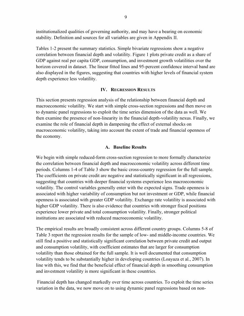
Financial Depth, shocks, and structural characteristics Theoretical considerations suggest that greater openness to trade may expose the country to external shocks, but leave it less vulnerable to internally generated shocks. Greater financial openness might in principle provide a mechanism by which a country could smooth shocks, but at the same time could expose it to greater volatility, as exogenous shifts in those capital flows disrupt economic activity. It has been argued that financial depth helps reduce the impact of external shocks particularly in environments of high exposure―that is, when trade and financial openness are high. We examine this issue by including a triple interaction between financial depth, openness, and shocks.

The results, reported in Table 8, confirm that the role of financial depth in dampening macroeconomic volatility depends on economies’ structural characteristics. Specifically, we find that while trade openness increases macroeconomic volatility, financial depth reduces the impact of terms-of-trade shocks on private consumption volatility in more open economies (Column 3). The results also point to a non-linear effect of external demand shocks on consumption volatility. Columns 6-7 illustrate that financial depth dampens the effect of external demand shocks on total and private consumption volatility in economies with greater trade openness. These results suggest that domestic financial depth plays an important role in stabilizing consumption in environments of high trade exposure.

Table 9 illustrates a similar positive role of financial depth in the case of financial openness. Although financial openness is associated with higher macroeconomic volatility, the impact of external demand and terms-of-trade shocks on consumption volatility, in particular, is reduced with greater financial depth (Columns 2-3, and 6-7). This finding suggests that

13

financial deepening plays an important role in attenuating the impact of external shocks on consumption volatility in more financially open economies.

V. ROBUSTNESS CHECKS

In this section we report evidence from a battery of robustness tests to show that the set of regressions presented in Tables 3-8 offers solid evidence that financial depth plays an important role in dampening volatility and in mitigating the negative effects of external shocks on consumption volatility, particularly in more open economies. Our results of a U shaped relationship between depth and volatility are also robust to alternative measures of financial depth. Alternative definition of volatility So far we have considered the standard deviation of the per-capita growth rate of the relevant variable as the measure of volatility. To assess the robustness of our results, we consider the deviation of the per-capita growth rate of output, consumption, and investment from its Hodrick-Prescott filter trend as the relevant measure. As can be seen from Table 10, our main results of a negative and significant relationship between financial depth and the volatility of growth, consumption, and investment still holds. Further, we confirm the existence of a non-monotonic relationship between depth and macroeconomic volatility.

Alternative definition of financial depth Our initial and preferred measure is private credit to GDP from banks and other financial institutions. Very similar results on the role of financial depth in dampening macroeconomic volatility are obtained when we consider three alternative measures of financial depth, all measured as percent of GDP: (i) total liquid liabilities, (ii) depository banks’ assets, and (iii) total deposits in financial institutions.

Table 11 presents the robustness test to the three different financial depth measures. In all instances, our result that greater financial depth reduces macroeconomic volatility is confirmed. Further, we find evidence of a non-linear relationship between finance and consumption and investment volatility. As in the regressions with private credit, the non-linear relationship with output volatility only holds for the sub-sample of advanced and emerging market countries. We also find evidence that financial depth plays an important role in mitigating the negative effects of exogenous shocks on macroeconomic volatility. Moreover, the result on complementarities between financial depth and country structural characteristics continue to hold across different measures (not reported here but available upon request).

Endogeneity issues At this point, the main qualification to our results would be the standard question of endogeneity. To examine whether this is a serious issue in our context, we make various tests

14

with the GMM methodology. The dynamic panel procedure using the GMM estimator controls for the potential endogeneity of all the explanatory variables and accounts explicitly for the biases induced by including the initial level of volatility in the regressions. It is true that the estimation procedure is valid only under the assumption of weak exogeneity of the explanatory variables. That is, they are assumed to be uncorrelated with future realizations of the error term. This assumption can be tested using a Hansen test of over-identification which evaluates the entire set of moment conditions in order to assess the overall level of the instruments. The results of the Hansen tests shown in Tables 3-12 indicates that the validity of the instruments cannot be rejected.8

As a robustness check, we re-estimated all regressions by substituting in the instrument matrix the third lag level of the explanatory variables for the second lag level. The results, not reported here but available upon request, show that lagging the set of internal instruments yields very similar estimates and ensures that our results are not biased by the presence of some omitted variables that could be correlated with financial depth and might have an independent effect on the next period’s volatility.

Finally, our empirical approach has several features that make it less vulnerable to a potential endogeneity bias. In addition to examining the direct effect of financial depth on volatility, we also focus on identifying contrasting volatility effects of real external shocks at different levels of financial depth, and for different degrees of openness of economies. Endogeneity is less of an issue with interaction terms than with single variables. Further, similar results are obtained for various measures of financial development, as well as for other measures of shocks (see below), and volatility.

Other robustness tests To further test the robustness of our results, we conducted a large number of additional tests and found that the results are indeed robust. Alternative definition of shocks To test that our results are robust to different external shocks, we also consider country-specific commodity price shocks, using the approach outlined in Aghion et al. (2010). This measure takes into account countries’ export characteristics, assigning a higher weight to large net commodity exporters for a given change in commodity prices. As can be seen from Table 12, the interaction term between financial depth and commodity price shocks is negative and significant, suggesting that while commodity shocks increase volatility, this effect is dampened in countries with deeper financial systems. Further, the results suggest

8 A second test examines whether the differenced error term is second-order serially correlated, a necessary condition for the consistency of the estimation. In all regressions, we can safely reject second-order serial correlation.

15

that this volatility dampening effect of finance is particularly pronounced for countries that exhibit greater trade and financial openness. Different time horizons The empirical results are broadly consistent across different time horizons (Table 13). When shorter time period are considered (3 years), we still find a negative and statistically significant relationship between private credit and macroeconomic volatility. However, given the large number of instruments, the power of the Hansen test of over-identification becomes low, resulting in very high p-values (close to 1). Still, the AR-2 test ensures validity of the specification and the results. Estimating the model for a longer 7 year period shows that the results remain significant, and that validity of instruments cannot be rejected.

Omission of continents and inclusion of other controls

Our main results remain stable and significant when sub-groups of countries are omitted in a systematic way. We also considered other control variables, such as including banking crises in all regressions, and replacing the Polity index with other measures of institutional quality. The thrust of our results remains essentially unchanged and is available upon request.

VI. CONCLUSIONS

This paper shed light on the ongoing debate on the effects of financial depth on macroeconomic volatility. It provides solid evidence that deeper financial systems dampen the volatility of output, consumption, and investment growth and can help cushion against adverse real external shocks. Our results also emphasize the consumption smoothing role of financial depth in countries with high trade and financial openness. Given the high welfare costs of volatility, and the more pronounced vulnerability of low-income and emerging market economies to sharp swings in commodity prices and the terms of trade, and trading partner volatility, our findings suggest that these countries can benefit from further financial deepening.

Our findings also suggest that there may be levels beyond which the beneficial effects on stability of financial depth diminish, and even become negative. This volatility amplifying effect of financial depth is largely driven by advanced economies and is also borne out from their experience in the global financial crisis. Several explanations have been put forward in the wake of the crisis for this non-linear effect of financial depth, ranging from a misallocation of funds, to the role of implicit safety nets in inducing aggressive risk-taking by banks.

Further empirical research is needed to gain insights into the factors that influence these threshold effects and the channels through which high levels of financial depth propagate and amplify instability. Policies could then be carefully calibrated for different economies in order to maximize the benefits of financial deepening in dampening macroeconomic volatility.

16

Figure 1. Financial Depth and Macroeconomic Volatility, 1974-2008 (with linear fitted lines and 95-percent confidence interval bands)

05

1015

Out

put V

ola

tility

0 50 100 150Private Credit to GDP

5-year PanelPer-cap GDP Growth Volatility

-10

010

2030

Tot

al C

onsu

mp

tion

Vo

latil

ity


5-year PanelPer-cap Private Consumption Growth Volatility

-10

010

2030

40P

riva

te C

ons

ump

tion

Vo

latil

ity


5-year PanelPer-cap Final Consumption Growth Volatility

020

4060

Inve

stm

ent

Vol

atil

ity


5-year PanelPer-cap Investment Growth Volatility

17

Figure 2. Marginal Effect of Private Credit on Final Consumption Volatility

Note: This figure shows the projected effect using the coefficients on both the ratio of private credit to GDP and its square in the final consumption volatility regression.

‐0.20

-0.15

-0.10

-0.05

0.00

0.05

0.10

0.15

0.20

0 20 40 60 80 100 120 140 160 180 200

Private Credit to GDP (in percent)

95% confidence band

18

Table 1. Summary Statistics (Five-year panel)

Variable Obs Mean Std. Dev. Min MaxSD of real per-capita growth of

GDP 880 3.47 3.37 0.06 34.39Final consumption 641 5.00 8.85 0.04 176.10Private consumption 663 5.90 10.31 0.01 178.62Investment 635 15.14 14.43 0.00 124.86

Real per-capita growth ofGDP 880 1.87 3.57 -21.96 31.64Final consumption 653 1.92 6.36 -23.61 129.38Private consumption 677 2.07 6.65 -19.85 131.25Investment 649 1.93 10.95 -83.19 56.72

Financial depth measuresLiquid liabilities 703 42.31 28.85 0.65 223.09Bank assets 717 44.04 38.85 1.99 241.28Private credit 728 39.74 37.44 1.39 195.77Deposits 718 37.28 30.52 1.74 211.73

ShocksPartner growth volatility 875 1.15 1.23 -2.48 11.93Terms-of-Trade volatility 850 0.03 6.85 -57.61 28.79Commodity export price volatility 818 0.04 0.23 -1.18 1.52Banking crisis 880 0.31 0.83 0.00 5.00

Other controlsTrade openness 723 54.99 39.74 8.88 346.82Financial openness 852 2.77 6.58 -14.41 92.24Inflation rate 752 29.77 140.66 -9.43 2282.40Government balance 819 -3.20 5.41 -24.78 27.83Polity index 827 -1.14 13.10 -88.00 10.00Real exchange rate volatility 822 7.68 15.73 0.00 164.00Initial real GDP per-capita 770 10.76 2.22 6.42 16.67

Table 2. Correlation Matrix (Five-year panel correlations between variables reported in Table 1)

GDP

growth

Final

consumption

growth

Private

consumption

growth

Investment

growth

GDP

volatility

Final

consumption

voaltility

Private

consumption

volatility

Investment

volatility

Liquid

liabilities

Bank

assets

Private

creditDeposits

Partner

Growth

volaitlity

Terms-of-

trade

volatility

Commodity

price

volatility

Banking

crisis

Trade

openness

Financial

openness

Inflation

rate

Government

balance

Polity

index

Real

exchange

rate

volatility

Initial

real GDP

per-

capita

GDP growth 1

Final consumption growth 0.6601 1

Private consumption growth 0.5793 0.9578 1

Investment growth 0.575 0.4264 0.3789 1

GDP volatility -0.0686 0.0109 0.0221 -0.0888 1

Final consumption volatility -0.0255 -0.0032 0.0148 0.0232 0.5378 1

Private consumption volatility -0.0336 0.0215 0.0408 -0.0062 0.4362 0.9211 1

Investment voaltility -0.2164 -0.1495 -0.1171 -0.0351 0.4429 0.4049 0.369 1

Liquid liabilities 0.1174 0.0894 0.0758 -0.0212 -0.2841 -0.3523 -0.3163 -0.3385 1

Bank assets 0.1146 0.08 0.0724 -0.0149 -0.2932 -0.3652 -0.3274 -0.3561 0.9178 1

Private credit 0.0918 0.069 0.0599 -0.0322 -0.2732 -0.3613 -0.3238 -0.3396 0.8319 0.9143 1

Deposits 0.1391 0.0971 0.0831 -0.01 -0.2924 -0.3566 -0.3176 -0.3444 0.982 0.9266 0.8644 1

Partner growth volaitlity 0.229 0.2018 0.1778 0.1042 0.0195 0.0875 0.144 0.0051 0.1471 0.1356 0.1492 0.1957 1

Terms-of-trade volatility 0.014 0.1493 0.1411 0.0596 0.1118 0.0771 0.0216 0.0068 -0.0078 0.018 0.0087 -0.0115 0.0812 1

Commodity price volatility 0.1215 0.273 0.2317 0.1308 0.0374 0.0003 0.0239 0.0781 0.0134 0.0019 -0.0033 0.0174 0.2104 0.4189 1

Banking crisis -0.1808 -0.198 -0.1811 -0.1052 0.1889 0.0567 0.028 0.1306 -0.0444 -0.0315 -0.0337 -0.0474 -0.1221 -0.0335 -0.0771 1

Trade openness 0.2363 0.1953 0.1647 0.0676 -0.0016 0.0165 0.0611 -0.0219 0.1903 0.1684 0.1722 0.2359 0.8311 0.0323 0.1708 -0.1148 1

Financial openness 0.3083 0.261 0.2234 0.1335 0.0863 0.0552 0.1075 -0.1014 0.2361 0.2938 0.2999 0.2383 0.3408 -0.017 0.0816 -0.0123 0.3398 1

Inflation rate -0.0851 -0.0457 -0.0096 -0.0095 0.1293 0.1227 0.205 0.0433 -0.1264 -0.1003 -0.1068 -0.1163 -0.0156 -0.0562 -0.0371 0.121 -0.0646 0.0119 1

Government balance 0.2463 0.2798 0.2147 0.1737 -0.1559 -0.18 -0.1986 -0.1496 0.0565 0.095 0.1604 0.094 0.2951 0.2386 0.4709 -0.0665 0.2598 0.1492 -0.0864 1

Polity index 0.3209 0.1843 0.1571 0.1808 -0.2738 -0.2855 -0.2794 -0.2937 0.311 0.3646 0.3408 0.3401 -0.0189 0.0675 -0.0075 -0.0147 0.0241 0.1218 -0.0669 0.1005 1

Real exchange rate volatility -0.1218 -0.0458 0.0007 -0.0604 0.2711 0.2717 0.3527 0.1784 -0.251 -0.226 -0.2384 -0.2451 -0.0112 -0.0362 -0.0238 0.2315 -0.0757 0.0107 0.8022 -0.1119 -0.1364 1

Initial real GDP per-capita -0.0248 -0.0264 -0.0248 0.0086 0.0274 0.0636 0.0272 0.0964 -0.0784 -0.0621 -0.0255 -0.0688 -0.0415 0.0401 -0.0166 0.0692 -0.1171 -0.0548 -0.0906 0.0721 -0.0142 -0.0819 1

19

Table 3. Financial Depth and Volatility: Cross-Section Regressions (OLS)

Dependent variable (volatility of growth rate of):

GDPFinal

ConsumptionPrivate

consumptionInvestment GDP

Final Consumption

Private Consumption

Investment

(1) (2) (3) (4) (5) (6) (7) (8)

(ln) Initial per-capita GDP 0.125 0.688*** 0.804** 1.240* 0.133 0.609* 0.712* 1.471(0.0962) (0.250) (0.318) (0.686) (0.0989) (0.321) (0.415) (0.940)

Per-capita growth 0.0119* 0.00688 0.0213 0.0622 -0.214 1.869*** 1.757*** -0.0759(0.00664) (0.0177) (0.0224) (0.0481) (0.157) (0.155) (0.197) (0.563)

Trade openness 0.151 1.812*** 1.712*** 0.0117 0.0270** 0.0208 0.0610 0.0779(0.139) (0.132) (0.165) (0.420) (0.0103) (0.0337) (0.0436) (0.0996)

Financial openness 0.105* 0.219 0.295 0.194 0.0508 0.0835 0.335 0.482(0.0592) (0.150) (0.191) (0.419) (0.0960) (0.312) (0.404) (0.939)

Polity index -0.0501* -0.155** -0.245** -0.434** -0.0206 -0.183* -0.238* -0.364(0.0278) (0.0747) (0.0951) (0.201) (0.0286) (0.0959) (0.124) (0.277)

Inflation -0.00487 0.00579 0.0408** -0.00810 -0.00261 0.0102 0.0430** -0.0135(0.00512) (0.0135) (0.0172) (0.0378) (0.00485) (0.0160) (0.0207) (0.0490)

Government balance 0.00177 -0.362* -0.495* -0.494 0.0280 -0.511* -0.603* -0.667(0.0758) (0.198) (0.251) (0.541) (0.0853) (0.279) (0.360) (0.817)

(sd) Real FX change 0.0488** 0.0254 0.0556 0.0193 0.0492** 0.00383 -0.0747 0.0321(0.0199) (0.0552) (0.0703) (0.149) (0.0188) (0.0658) (0.0851) (0.192)

Private Credit -0.0315*** -0.0682*** -0.0793*** -0.125** -0.0119*** -0.106** -0.152** -0.102(0.00843) (0.0222) (0.0281) (0.0605) (0.00327) (0.0452) (0.0584) (0.131)

Constant 2.667* -4.493 -5.316 5.518 2.729* -4.744 -5.600 1.599(1.347) (3.454) (4.394) (9.521) (1.510) (4.768) (6.165) (14.22)

Observations 110 110 110 110 76 76 76 76

R-squared 0.424 0.756 0.682 0.235 0.419 0.771 0.694 0.130

*** p<0.01, ** p<0.05, * p<0.1

FULL SAMPLE EMERGING & LICs

Standard errors in parentheses

20

Table 4. Financial Depth and Volatility: Panel Regressions (GMM)


GDPFinal

ConsumptionPrivate


Final Consumption

Private Consumption

Investment

(1) (2) (3) (4) (9) (10) (11) (12)

Lagged dependent variable 0.0238 0.0274 0.115 0.0180 -0.0354 0.0252 0.0999 0.00579(0.0749) (0.0396) (0.113) (0.204) (0.0809) (0.0377) (0.102) (0.207)

Per-capita growth -0.103 -0.117 -0.0835 0.103 -0.168* -0.326 -0.128 0.109(0.102) (0.291) (0.232) (0.157) (0.0955) (0.197) (0.227) (0.204)

(ln) Initial per-capita GDP 0.0594 0.139 0.193 0.790* -0.0212 0.0462 0.0123 0.625(0.0729) (0.168) (0.202) (0.450) (0.0899) (0.212) (0.264) (0.546)

Trade openness 0.00498 0.0101 0.0228 0.0318* 0.00637 0.0293 0.0614* 0.0491(0.00486) (0.0128) (0.0180) (0.0178) (0.00790) (0.0235) (0.0321) (0.0372)

Financial openness 0.0888 0.141** 0.238* 0.0346 0.0320 0.105 0.324 0.110(0.0577) (0.0697) (0.138) (0.0947) (0.0246) (0.104) (0.273) (0.170)

Polity index -0.0329** -0.0708** -0.0970*** -0.137 -0.0151 -0.0564* -0.0874* -0.137(0.0145) (0.0323) (0.0364) (0.126) (0.0168) (0.0314) (0.0493) (0.107)

Inflation 0.00179 -0.00158 -0.00374 -0.0149 0.000583 0.000445 -0.00200 -0.0123(0.00195) (0.00351) (0.00873) (0.0165) (0.00173) (0.00317) (0.00851) (0.0152)

Government balance -0.00129 -0.0615 -0.352 -0.567** -0.102 -0.00825 -0.425 -0.593(0.0555) (0.0953) (0.216) (0.257) (0.0887) (0.160) (0.307) (0.371)

(sd) Real FX change 0.000271 0.0410 0.118 0.206 0.0156 0.0146 0.0942 0.131(0.0269) (0.0447) (0.120) (0.165) (0.0239) (0.0438) (0.112) (0.161)

Private credit -0.0149** -0.0362*** -0.0455*** -0.0631*** -0.0154* -0.0618** -0.109** -0.110**(0.00650) (0.0103) (0.0149) (0.0231) (0.00877) (0.0255) (0.0424) (0.0489)

Constant 1.299 1.882 -0.0445 -0.728 2.542** 3.416 1.082 0.882(1.071) (2.167) (2.851) (4.127) (1.242) (2.517) (3.969) (6.282)

Observations 628 485 506 481 437 326 326 326Number of Countries 110 110 110 110 79 79 79 79Time Dummies YES YES YES YES YES YES YES YESHansen test p-value 0.272 0.604 0.305 0.677 0.997 0.943 0.883 0.939A-B AR(2) test p-value 0.865 0.294 0.138 0.893 0.683 0.537 0.155 0.988

Standard errors in parentheses*** p<0.01, ** p<0.05, * p<0.1

FULL SAMPLE EMERGING & LICs

21

Table 5. Non-linear Relationship Between Financial Depth and Volatility: Panel Regressions (GMM)


GDPFinal

ConsumptionPrivate

ConsumptionInvestment

(1) (2) (3) (4)

Lagged dependent variable -0.00175 0.0232 0.107 0.0261(0.0778) (0.0388) (0.105) (0.187)

Per-capita growth -0.120 -0.167 -0.0967 0.0241(0.101) (0.322) (0.166) (0.159)

(ln) Initial per-capita GDP 0.0415 0.131 0.131 0.471(0.106) (0.149) (0.206) (0.336)

Trade openness 0.00686 0.0141* 0.0284 0.0477***(0.00440) (0.00833) (0.0188) (0.0177)

Financial openness 0.0955 0.154* 0.243 0.0545(0.0697) (0.0895) (0.151) (0.0989)

Polity index -0.0228 -0.0610** -0.0858*** -0.100(0.0181) (0.0289) (0.0298) (0.105)

Inflation 0.00203 -0.00152 -0.00421 -0.0112(0.00203) (0.00358) (0.00779) (0.0120)

Government balance -0.0180 -0.118 -0.398** -0.537**(0.0559) (0.0967) (0.183) (0.257)

(sd) Real FX change -0.00702 0.0334 0.110 0.109(0.0276) (0.0456) (0.110) (0.122)

Private credit (PC) -0.0397* -0.0985*** -0.126*** -0.326**(0.0214) (0.0346) (0.0446) (0.126)

PC Squared 0.000135 0.000371* 0.000529** 0.00154**(0.000103) (0.000198) (0.000254) (0.000712)

Constant 2.061 3.153 1.812 8.299(1.344) (2.245) (2.906) (5.504)

Fin Depth Joint Eff p-value 0.0378 1.69e-05 0.00205 0.00243Threshold Value 132.9 118.6 106.0SE of Threshold Value 27.78 20.10 11.06Threshold 95% CI (78.5,187.4) (79.2,158.0) (84.3,127.7)Observations 628 485 506 481Number of Countries 110 110 110 110Time Dummies YES YES YES YESHansen test p-value 0.697 0.712 0.757 0.737A-B AR(2) test p-value 0.750 0.333 0.153 0.783

Standard errors in parentheses*** p<0.01, ** p<0.05, * p<0.1

22

Table 6. Financial Depth, Shocks, and Macroeconomic Volatility: Panel-Regressions (GMM)


(1) (2) (3) (4) (5) (6) (7) (8) (9) (10) (11) (12) (13) (14) (15) (16)

Lagged dependent Variable -0.148 -0.139 -0.0516 0.00697 -0.00426 -0.00245 0.133 0.286** 0.0452 0.0526 0.224** 0.376*** -0.112 -0.116 -0.110 0.0556

(0.128) (0.128) (0.127) (0.0725) (0.0141) (0.0140) (0.186) (0.130) (0.0612) (0.0633) (0.0933) (0.0692) (0.154) (0.137) (0.185) (0.195)

Per-capita growth 0.00797 -0.00201 -0.0259 -0.0401 0.0779 0.0542 0.0202 -0.00665 0.0126 0.00169 0.0371 0.0306 0.221 0.246 0.242 0.0150

(0.121) (0.108) (0.127) (0.0879) (0.353) (0.338) (0.295) (0.304) (0.376) (0.378) (0.292) (0.183) (0.184) (0.197) (0.163) (0.187)

(ln) Initial per-capita GDP 0.115 0.136 0.113 0.0242 0.257 0.260 0.137 0.0799 0.227 0.190 0.170 0.0795 1.029*** 0.999*** 0.970*** 0.433

(0.0966) (0.0863) (0.0839) (0.0899) (0.174) (0.182) (0.187) (0.141) (0.208) (0.194) (0.197) (0.144) (0.362) (0.337) (0.339) (0.354)

Trade openness 0.0117** 0.00103 0.00753* -0.00144 0.00703 0.00576 0.00470 0.00518 0.0190 0.0169 0.0201 0.0157 0.0397* 0.0183 0.0400** 0.0185

(0.00476) (0.00523) (0.00414) (0.00411) (0.00726) (0.00698) (0.00639) (0.00580) (0.0127) (0.0132) (0.0126) (0.0138) (0.0212) (0.0271) (0.0196) (0.0221)

Financial openness 0.0420 0.0443 0.0309 0.0688 0.0820** 0.0729 0.0668 0.111 0.204* 0.215* 0.172 0.165 -0.0346 -0.0677 -0.0662 0.0363

(0.0577) (0.0562) (0.0564) (0.0508) (0.0368) (0.0450) (0.0471) (0.0711) (0.106) (0.119) (0.122) (0.109) (0.184) (0.191) (0.197) (0.0828)

Polity index -0.0472** -0.0430** -0.0414** -0.0298 -0.0662* -0.0643* -0.0349 -0.0402 -0.0494 -0.0497 -0.0423 -0.0615** -0.170 -0.171 -0.151 -0.118

(0.0188) (0.0192) (0.0185) (0.0191) (0.0355) (0.0333) (0.0476) (0.0253) (0.0520) (0.0481) (0.0418) (0.0281) (0.109) (0.105) (0.109) (0.105)

Inflation -0.0113 -0.00874 -0.00681 0.00199 0.0132 0.0149 0.00799 -0.000423 0.0107 0.00874 0.00681 -0.00146 -0.0351* -0.0378* -0.0348 -0.00865

(0.0109) (0.00936) (0.00626) (0.00191) (0.0198) (0.0206) (0.0141) (0.00269) (0.0204) (0.0197) (0.0194) (0.00612) (0.0195) (0.0200) (0.0234) (0.0103)

Government balance -0.0558 -0.0590 -0.0200 -0.0136 -0.195* -0.201** -0.103 -0.00982 -0.640*** -0.633*** -0.574** -0.299 -1.105*** -1.142*** -1.078*** -0.432*

(0.0716) (0.0709) (0.0668) (0.0620) (0.104) (0.0988) (0.0764) (0.0938) (0.203) (0.187) (0.259) (0.255) (0.236) (0.230) (0.255) (0.259)

(sd) Real FX change 0.108 0.102* 0.117** 0.000278 0.100 0.105 0.0613 0.0156 0.124 0.128 0.0936 0.0811 0.406* 0.469* 0.460* 0.0788

(0.0678) (0.0605) (0.0449) (0.0245) (0.0794) (0.0796) (0.0754) (0.0308) (0.108) (0.125) (0.112) (0.0860) (0.238) (0.246) (0.251) (0.116)

(sd) Term-of-Trade Growth 0.0392* 0.0533** 0.0899** 0.125** 0.120** 0.165*** 0.114 0.175**

(0.0211) (0.0223) (0.0415) (0.0547) (0.0536) (0.0565) (0.122) (0.0828)

(sd) Partner Growth 1.373* 1.059 0.429 0.363 0.411 0.744 3.438 3.166

(0.757) (0.642) (0.501) (0.705) (0.425) (0.609) (3.633) (2.696)

Banking crisis 0.382* 0.271 0.0918 0.296 0.519 -0.239 0.123* 2.818*

(0.228) (0.232) (0.320) (0.456) (0.406) (0.711) (0.0651) (1.458)

Private credit -0.0146***-0.0160*** -0.0113** -0.0108** -0.0217** -0.0196* -0.0195* -0.0227* -0.0268* -0.0278** -0.0178 -0.0157 -0.0732** -0.0731** -0.0517* -0.0706***

(0.00494) (0.00604) (0.00559) (0.00544) (0.0109) (0.0106) (0.0112) (0.0118) (0.0140) (0.0133) (0.0119) (0.0100) (0.0337) (0.0353) (0.0296) (0.0222)

Constant -0.409 -0.393 -0.678 1.395 -0.806 -0.977 -0.127 0.718 -1.553 -1.282 -3.183 -0.0157 -3.153 -2.847 -4.087 2.495

(1.529) (1.413) (1.437) (1.016) (3.112) (3.219) (3.083) (2.102) (3.756) (3.513) (3.454) (0.0100) (5.783) (5.411) (5.270) (4.054)

Observations 628 628 614 614 485 485 478 478 506 506 499 499 481 481 474 474

Number of countries 110 110 108 108 108 108 108 108 108 108 108 108 108 108 108 108

Time Dummies YES YES YES YES YES YES YES YES YES YES YES YES YES YES YES YES

Hansen test p-value 0.463 0.439 0.283 0.723 0.834 0.735 0.647 0.693 0.840 0.795 0.476 0.965 0.745 0.768 0.791 0.733

A-B AR(2) test p-value 0.401 0.228 0.790 0.292 0.387 0.355 0.253 0.341 0.237 0.206 0.131 0.264 0.614 0.597 0.635 0.746


*** p<0.01, ** p<0.05, * p<0.1

Final ConsumptionGDP Private Consumption Investment

23

Table 7. Interacting Financial Depth and External Shocks: Panel-Regressions (GMM)


GDPFinal

ConsumptionPrivate

ConsumptionInvestment GDP

Final Consumption

Private Consumption

Investment

(1) (2) (3) (4) (5) (6) (7) (8)

Lagged dependent variable 0.0383 0.268** 0.376*** 0.0132 0.00868 0.0337 0.111 0.0908(0.0808) (0.134) (0.0681) (0.208) (0.0703) (0.0433) (0.109) (0.185)

Per-capita growth -0.0113 -0.0184 0.0613 0.0162 -0.0829 -0.115 -0.0988 0.105(0.150) (0.280) (0.177) (0.164) (0.0930) (0.285) (0.199) (0.186)

(log) Initial per-capita GDP 0.0528 0.103 0.179 0.618 0.0749 0.225 0.238 0.649*(0.0856) (0.135) (0.184) (0.390) (0.0810) (0.166) (0.198) (0.356)

Trade openness (TO) 0.00483 0.00925 0.0230* 0.0283* -0.00188 0.00621 0.0210 0.00381(0.00462) (0.00735) (0.0123) (0.0162) (0.00340) (0.00804) (0.0137) (0.0171)

Financial openness (FO) 0.0526 0.0729 0.146** -0.0220 0.0893 0.145 0.218* 0.0261(0.0328) (0.0517) (0.0712) (0.106) (0.0631) (0.0894) (0.124) (0.0831)

Polity index -0.0257 -0.0430 -0.0627** -0.139 -0.0272* -0.0743** -0.0950** -0.129(0.0164) (0.0263) (0.0297) (0.111) (0.0139) (0.0294) (0.0368) (0.110)

Inflation 0.000579 0.000573 -0.000638 -0.0143 0.00171 -0.000641 -0.00143 -0.0162(0.00209) (0.00239) (0.00496) (0.0147) (0.00192) (0.00448) (0.00855) (0.0137)

Government Balance -0.0189 -0.0255 -0.282 -0.322 -0.0357 -0.0480 -0.335* -0.568**(0.0551) (0.0869) (0.179) (0.301) (0.0598) (0.104) (0.193) (0.257)

(sd) Real FX change 0.0146 0.00499 0.0592 0.172 0.00241 0.0287 0.104 0.194(0.0299) (0.0301) (0.0601) (0.139) (0.0282) (0.0575) (0.117) (0.135)

Private credit (PC) -0.00328 -0.00868 -0.00795 -0.00901 -0.0152** -0.0335*** -0.0191 -0.0793***(0.00584) (0.0125) (0.0163) (0.0289) (0.00677) (0.00913) (0.0180) (0.0275)

(sd) Terms-of-Trade Growth 0.128*** 0.187** 0.305*** 0.477***(0.0395) (0.0783) (0.0997) (0.178)

(sd) Partner Growth 1.237 2.584 6.303** 1.983(0.872) (1.940) (2.717) (5.278)

PC x (sd) ToT Growth -0.00338*** -0.00332* -0.00583** -0.0132**(0.00117) (0.00174) (0.00280) (0.00612)

PC x (sd) Partner Growth -0.00200 -0.0255 -0.0670** 0.0272(0.00773) (0.0183) (0.0311) (0.0449)

Constant 0.175 -0.597 -4.745 -1.302 1.088 0.482 -2.454 1.471(1.417) (2.123) (3.264) (4.120) (1.188) (2.448) (3.654) (4.025)

Observations 614 478 499 474 628 485 506 481Number of Countries 108 108 108 108 110 110 110 110Time Dummies YES YES YES YES YES YES YES YESHansen test p-value 0.768 0.883 0.904 0.830 0.802 0.840 0.872 0.850A-B AR(2) test p-value 0.849 0.142 0.0379 0.952 0.560 0.313 0.178 0.572Standard errors in parentheses*** p<0.01, ** p<0.05, * p<0.1

TERMS-OF-TRADE GROWTH PARTNER GROWTH

24

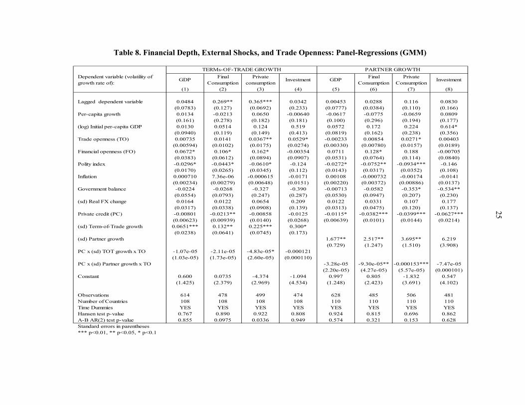
Table 8. Financial Depth, External Shocks, and Trade Openness: Panel-Regressions (GMM)


GDPFinal

ConsumptionPrivate


Final Consumption

Private Consumption

Investment

(1) (2) (3) (4) (5) (6) (7) (8)

Lagged dependent variable 0.0484 0.269** 0.365*** 0.0342 0.00453 0.0288 0.116 0.0830(0.0783) (0.127) (0.0692) (0.233) (0.0777) (0.0384) (0.110) (0.166)

Per-capita growth 0.0134 -0.0213 0.0650 -0.00640 -0.0617 -0.0775 -0.0659 0.0809(0.161) (0.278) (0.182) (0.181) (0.100) (0.296) (0.194) (0.177)

(log) Initial per-capita GDP 0.0130 0.0514 0.124 0.519 0.0572 0.172 0.224 0.614*(0.0940) (0.119) (0.149) (0.413) (0.0819) (0.162) (0.238) (0.356)

Trade openness (TO) 0.00735 0.0141 0.0367** 0.0529* -0.00233 0.00854 0.0271* 0.00403(0.00594) (0.0102) (0.0175) (0.0274) (0.00330) (0.00780) (0.0157) (0.0189)

Financial openness (FO) 0.0672* 0.106* 0.162* -0.00354 0.0711 0.128* 0.188 -0.00705(0.0383) (0.0612) (0.0894) (0.0907) (0.0531) (0.0764) (0.114) (0.0840)

Polity index -0.0296* -0.0443* -0.0610* -0.124 -0.0272* -0.0752** -0.0934*** -0.146(0.0170) (0.0265) (0.0345) (0.112) (0.0143) (0.0317) (0.0352) (0.108)

Inflation 0.000710 7.36e-06 -0.000615 -0.0171 0.00108 -0.000732 -0.00174 -0.0141(0.00234) (0.00279) (0.00648) (0.0151) (0.00220) (0.00372) (0.00886) (0.0137)

Government balance -0.0224 -0.0268 -0.327 -0.390 -0.00713 -0.0582 -0.353* -0.534**(0.0554) (0.0793) (0.247) (0.287) (0.0530) (0.0947) (0.207) (0.230)

(sd) Real FX change 0.0164 0.0122 0.0654 0.209 0.0122 0.0331 0.107 0.177(0.0317) (0.0338) (0.0908) (0.139) (0.0313) (0.0475) (0.120) (0.137)

Private credit (PC) -0.00801 -0.0213** -0.00858 -0.0125 -0.0115* -0.0382*** -0.0399*** -0.0627***(0.00623) (0.00939) (0.0140) (0.0268) (0.00639) (0.0101) (0.0144) (0.0214)

(sd) Term-of-Trade growth 0.0651*** 0.132** 0.225*** 0.300*(0.0238) (0.0641) (0.0745) (0.173)

(sd) Partner growth 1.677** 2.517** 3.695** 6.219(0.729) (1.247) (1.510) (3.908)

PC x (sd) TOT growth x TO -1.07e-05 -2.11e-05 -4.83e-05* -0.000121(1.03e-05) (1.73e-05) (2.60e-05) (0.000110)

PC x (sd) Partner growth x TO -3.28e-05 -9.30e-05** -0.000153*** -7.47e-05(2.20e-05) (4.27e-05) (5.57e-05) (0.000101)

Constant 0.600 0.0735 -4.374 -1.094 0.997 0.805 -1.832 0.547(1.425) (2.379) (2.969) (4.534) (1.248) (2.423) (3.691) (4.102)

Observations 614 478 499 474 628 485 506 481Number of Countries 108 108 108 108 110 110 110 110Time Dummies YES YES YES YES YES YES YES YESHansen test p-value 0.767 0.890 0.922 0.808 0.924 0.815 0.696 0.862A-B AR(2) test p-value 0.855 0.0975 0.0336 0.949 0.574 0.321 0.153 0.628Standard errors in parentheses*** p<0.01, ** p<0.05, * p<0.1

TERMs-OF-TRADE GROWTH PARTNER GROWTH

25

Table 9. Financial Depth, External Shocks, and Financial Openness: Panel-Regressions (GMM)

Dependent variable (volatility of growth rate of): GDP

Final

Consumption

Private

Consumption Investment GDP

Final

Consumption

Private

Consumption Investment

(1) (2) (3) (4) (5) (6) (7) (8)

Lagged dependent variable 0.107 0.304** 0.359*** 0.0459 0.0466 0.0302 0.102 0.0713

(0.0705) (0.126) (0.0773) (0.215) (0.0784) (0.0440) (0.0914) (0.177)

Per-capita growth 0.106 0.0318 0.0106 -0.0322 -0.102 -0.241 -0.253 0.105

(0.184) (0.217) (0.161) (0.165) (0.0983) (0.276) (0.170) (0.172)

(log) Initial per-capita GDP 0.0471 0.0721 0.137 0.628* 0.0444 0.174 0.296 0.650*

(0.0873) (0.152) (0.159) (0.342) (0.0946) (0.175) (0.205) (0.371)

Trade openness 0.00217 0.00483 0.0176* 0.0284** -0.00366 0.00304 0.0164 0.00172

(0.00356) (0.00644) (0.00991) (0.0132) (0.00346) (0.00694) (0.0122) (0.0182)

Financial openness (FO) 0.0918* 0.203** 0.402* 0.0723 0.110 0.318** 0.553*** 0.0529

(0.0468) (0.0807) (0.209) (0.155) (0.0882) (0.147) (0.209) (0.135)

Polity index -0.0398* -0.0430* -0.0665* -0.120 -0.0263** -0.0740** -0.0956** -0.138

(0.0209) (0.0254) (0.0344) (0.105) (0.0128) (0.0305) (0.0376) (0.0999)

Inflation -0.000159 7.25e-05 -0.000143 -0.0125 0.00163 -0.000307 -0.00145 -0.0139

(0.00229) (0.00273) (0.00590) (0.0127) (0.00210) (0.00385) (0.00678) (0.0141)

Government Balance -0.0445 -0.0741 -0.336 -0.316 -0.0111 -0.0440 -0.336* -0.488*

(0.0579) (0.0916) (0.227) (0.268) (0.0587) (0.130) (0.199) (0.252)

(sd) Real FX change 0.0304 0.00750 0.0521 0.159 0.00135 0.0216 0.0806 0.183

(0.0327) (0.0378) (0.0824) (0.124) (0.0296) (0.0455) (0.0879) (0.148)

Private Credit (PC) -0.00266 -0.0193** -0.00860 -0.0439** -0.0129** -0.0348*** -0.0389*** -0.0615**

(0.00517) (0.00816) (0.0118) (0.0203) (0.00622) (0.0110) (0.0110) (0.0238)

(sd) Term of Trade growth (TOT) 0.0594** 0.127** 0.191*** 0.175*

(0.0239) (0.0604) (0.0612) (0.0923)

PC x FO x (sd) ToT -8.33e-05 -0.000247* -0.000658* -0.000249

(7.21e-05) (0.000131) (0.000379) (0.000368)

(sd) Partner growth 1.445** 2.611** 4.771*** 4.907*

(0.629) (1.182) (1.771) (2.889)

PC x (sd) Partner growth x TO -0.000393 -0.00190* -0.00363** -0.000361

(0.000424) (0.00100) (0.00172) (0.00132)

Constant -0.265 -0.336 -3.726 0.416 1.230 0.852 -3.194 0.217

(1.662) (2.793) (2.728) (3.792) (1.515) (2.556) (3.222) (4.594)

Observations 614 478 499 474 628 485 506 481

Number of Countries 108 108 108 108 110 110 110 110

Time Dummies YES YES YES YES YES YES YES YES

Hansen test p-value 0.821 0.793 0.934 0.815 0.850 0.729 0.892 0.907

A-B AR(2) test p-value 0.676 0.0654 0.0312 0.891 0.877 0.350 0.277 0.655


*** p<0.01, ** p<0.05, * p<0.1

TERMS-OF-TRADE GROWTH PARTNER GROWTH

26

Table 10. Financial Depth and HP-filtered Volatility: Panel-Regressions (GMM)

(1) (2) (3) (4) (5) (6) (7) (8)

Lagged dependent variable 0.207*** 0.177** 0.264** 0.229*** 0.383*** 0.342*** 0.132 0.0666(0.0667) (0.0828) (0.107) (0.0856) (0.0902) (0.0881) (0.158) (0.127)

Per-capita growth -0.0572 -0.0672 0.157* 0.200*** 0.145** 0.179*** 0.0810 0.0549(0.0439) (0.0634) (0.0813) (0.0721) (0.0719) (0.0544) (0.111) (0.101)

(log) Initial per-capita GDP 0.0307 0.0183 0.133 0.132 0.161* 0.0854 0.504** 0.194(0.0438) (0.0500) (0.0814) (0.0967) (0.0814) (0.111) (0.195) (0.234)

Trade openness 0.00286 0.00386 0.00471 0.00695 0.0137** 0.0154** 0.0139 0.0256**(0.00265) (0.00281) (0.00434) (0.00512) (0.00637) (0.00606) (0.00899) (0.0116)

Financial openness 0.0481 0.0519 0.0806* 0.0699 0.121 0.121* 0.0568 0.0271(0.0461) (0.0404) (0.0483) (0.0461) (0.0763) (0.0612) (0.0528) (0.0714)

Polity index -0.0193** -0.0121 -0.0421*** -0.0378*** -0.0582*** -0.0516*** -0.114* -0.0816(0.00902) (0.00770) (0.0149) (0.0143) (0.0180) (0.0178) (0.0654) (0.0639)

Inflation -7.62e-05 0.000224 -0.000673 -0.000882 -0.00163 -0.00142 -0.00348 -0.000797(0.00145) (0.00110) (0.00197) (0.00231) (0.00489) (0.00515) (0.00748) (0.00682)

Government Balance -0.0114 -0.0173 -0.0995* -0.133** -0.308* -0.313** -0.304 -0.371**(0.0350) (0.0310) (0.0508) (0.0577) (0.166) (0.128) (0.190) (0.148)

(sd) Real FX change 0.0113 0.00487 0.0185 0.0211 0.0647 0.0630 0.0590 -0.00240(0.0188) (0.0143) (0.0250) (0.0306) (0.0611) (0.0607) (0.0886) (0.0779)

Private Credit -0.00743* -0.0282** -0.0247*** -0.0682*** -0.0214*** -0.0859*** -0.0494*** -0.280***(0.00414) (0.0112) (0.00640) (0.0182) (0.00695) (0.0243) (0.0187) (0.0703)

PC Squared 0.000117** 0.000316*** 0.000429*** 0.00142***(5.31e-05) (9.93e-05) (0.000134) (0.000400)

Constant 0.476 1.103 -0.956 -0.443 -2.723** -0.874 -1.275 7.265**(0.640) (0.797) (0.996) (1.176) (1.260) (1.561) (2.256) (3.586)

Fin Depth Joint Eff p-value 0.0188 0.000253 0.00164 0.000161Threshold Value 120.6 107.7 100.1 98.39SE of Threshold Value 11.78 8.864 7.814 5.984Threshold 95% CI (97.6,143.7) (90.3,125.1) (84.7,115.4) (86.7,110.1)Observations 628 628 565 565 577 577 563 563Number of Countries 110 110 110 110 110 110 110 110Time Dummies YES YES YES YES YES YES YES YESHansen test p-value 0.247 0.723 0.270 0.897 0.299 0.830 0.430 0.884A-B AR(2) test p-value 0.891 0.941 0.786 0.75 0.113 0.101 0.475 0.530Standard errors in parentheses*** p<0.01, ** p<0.05, * p<0.1

GDP Final Consumption Private Consumption InvestmentDependent variable (deviation from HP filter in growth of):

27

Table 11. Alternative Measures of Financial Depth: Panel-Regressions (GMM)

(1) (2) (3) (4) (5) (6) (7) (8) (9) (10) (11) (12)

Lagged dependent variable 0.0417 -0.00175 -0.0184 0.0132 0.0189 0.0183 0.0903 0.0910 0.0950 0.0295 0.0899 -0.0148(0.0974) (0.0776) (0.0690) (0.0311) (0.0348) (0.0341) (0.108) (0.0996) (0.104) (0.196) (0.175) (0.181)

Per-capita growth -0.139 -0.125 -0.101 -0.154 -0.112 -0.127 -0.146 -0.0768 -0.0936 0.00222 -0.0330 -0.00973(0.113) (0.116) (0.111) (0.309) (0.305) (0.318) (0.224) (0.201) (0.233) (0.170) (0.148) (0.159)

(log) Initial per-capita GDP 0.0178 0.0374 0.0537 0.0344 0.103 0.0397 0.0139 0.0401 0.00706 0.275 0.310 0.184(0.0877) (0.0841) (0.0879) (0.167) (0.149) (0.181) (0.233) (0.184) (0.257) (0.397) (0.320) (0.371)

Trade openness 0.00784* 0.00642 0.00718 0.0154* 0.0118 0.0166* 0.0341** 0.0352** 0.0363** 0.0494** 0.0453*** 0.0568***(0.00463) (0.00478) (0.00473) (0.00911) (0.00907) (0.00891) (0.0169) (0.0161) (0.0173) (0.0213) (0.0170) (0.0184)

Financial openness 0.0860 0.0916 0.0830 0.146 0.141* 0.131 0.200* 0.245* 0.209 0.0219 0.0750 0.0139(0.0533) (0.0645) (0.0536) (0.0889) (0.0835) (0.0858) (0.119) (0.127) (0.130) (0.0968) (0.0814) (0.0876)

Polity index -0.0213 -0.0226 -0.0265* -0.0616* -0.0663** -0.0640** -0.0887** -0.0735* -0.0895** -0.121 -0.0860 -0.100(0.0147) (0.0181) (0.0155) (0.0326) (0.0314) (0.0297) (0.0376) (0.0374) (0.0395) (0.102) (0.100) (0.0894)

Inflation 0.00107 0.00144 0.00149 -0.00298 -0.00171 -0.00270 -0.00435 -0.00365 -0.00552 -0.0157 -0.0113 -0.0164(0.00193) (0.00184) (0.00162) (0.00384) (0.00401) (0.00392) (0.00833) (0.00845) (0.00924) (0.0127) (0.0119) (0.0130)

Government Balance -0.0228 -0.0231 -0.0171 -0.159 -0.0646 -0.114 -0.466** -0.424* -0.406* -0.611** -0.632** -0.591**(0.0596) (0.0593) (0.0581) (0.102) (0.0938) (0.105) (0.228) (0.219) (0.233) (0.299) (0.300) (0.249)

(sd) Real FX change 0.000914 -0.000299 -0.00141 0.0470 0.0422 0.0451 0.108 0.105 0.121 0.167 0.120 0.173(0.0247) (0.0257) (0.0258) (0.0480) (0.0495) (0.0505) (0.108) (0.105) (0.119) (0.119) (0.119) (0.125)

Liquid Liabilities (LL) -0.0505* -0.126** -0.166** -0.309***(0.0286) (0.0583) (0.0661) (0.113)

LL Squared 0.000178 0.000477* 0.000646** 0.00120**(0.000129) (0.000274) (0.000298) (0.000577)

Bank Assets (BA) -0.0321** -0.0821*** -0.142*** -0.248***(0.0155) (0.0251) (0.0461) (0.0944)

BA Squared 8.64e-05 0.000259** 0.000536** 0.000943**(6.65e-05) (0.000111) (0.000207) (0.000467)

Deposits (DP) -0.0431* -0.104** -0.144** -0.357***(0.0227) (0.0474) (0.0579) (0.107)

DP Squared 0.000156 0.000388* 0.000595** 0.00154**(0.000106) (0.000227) (0.000287) (0.000591)

Constant 2.855** 2.156* 2.091* 5.769* 3.493 4.332 5.625 3.557 3.718 13.07* 9.416* 14.30**(1.223) (1.226) (1.246) (2.955) (2.349) (2.736) (4.242) (3.081) (3.795) (7.241) (5.205) (6.535)

Fin Depth Joint Eff p-value 0.00266 0.0111 0.00491 2.25e-06 4.30e-06 1.91e-05 0.00435 0.000787 0.00332 0.00182 0.00117 0.000652Threshold Value 132.5 158.3 134.3 128.6 132.6 120.6 129.2 131.4 115.8SE of Threshold Value 16.23 22.78 19.07 11.30 11.93 12.66 20.25 18.93 14.88Threshold 95% CI (100.7,164.3) (113.6,202.9) (96.9,171.6) (106.4,150.7) (109.2,156.0) (95.8,145.5) (89.5,168.9) (94.3,168.5) (86.7,145.0)Observations 610 621 621 472 480 480 493 501 501 468 476 476Number of Countries 109 110 110 108 109 109 108 110 110 108 109 109Time Dummies YES YES YES YES YES YES YES YES YES YES YES YESHansen test p-value 0.796 0.695 0.690 0.945 0.715 0.816 0.808 0.821 0.705 0.859 0.902 0.923A-B AR(2) test p-value 0.611 0.740 0.760 0.321 0.272 0.313 0.169 0.161 0.154 0.803 0.575 0.963Standard errors in parentheses

*** p<0.01, ** p<0.05, * p<0.1


GDP Final Consumption Private Consumption Investment

28

Table 12. Financial Depth and Commodity Export Shocks: Panel-Regressions (GMM)

GDP

Final

Consumption

Private

Consumption Investment GDP

Final

Consumption

Private

Consumption Investment

(1) (2) (3) (4) (5) (6) (7) (8)

Lagged dependent variable -0.00725 0.0224 0.101 0.0479 0.00939 0.0207 0.0942 0.0431

(0.0950) (0.0350) (0.0930) (0.188) (0.0758) (0.0328) (0.0894) (0.184)

Per-capita growth -0.0156 0.0106 0.0433 0.110 -0.0699 -0.0850 -0.0704 0.136

(0.118) (0.263) (0.221) (0.211) (0.112) (0.296) (0.204) (0.196)

(log) Initial per-capita GDP 0.0411 0.104 0.0691 0.545 0.0143 0.107 0.122 0.644*

(0.0912) (0.171) (0.186) (0.381) (0.0850) (0.161) (0.189) (0.361)

Trade openness (TO) 0.00347 0.0125 0.0348** 0.0219 0.000666 0.0132 0.0330* 0.0204

(0.00510) (0.00959) (0.0175) (0.0238) (0.00409) (0.00986) (0.0178) (0.0195)

Financial openness (FO) 0.0851* 0.133 0.219 0.0337 0.106 0.221* 0.352** 0.0516

(0.0490) (0.0807) (0.141) (0.0955) (0.0654) (0.119) (0.174) (0.0859)

Polity index -0.0279* -0.0723** -0.0937*** -0.146 -0.0262** -0.0707** -0.0907*** -0.160

(0.0145) (0.0304) (0.0340) (0.107) (0.0130) (0.0279) (0.0291) (0.114)

Inflation 0.00157 -0.000610 -0.00288 -0.0137 0.00148 0.000690 -0.00101 -0.0144

(0.00205) (0.00296) (0.00852) (0.0141) (0.00210) (0.00317) (0.00676) (0.0155)

Government balance -0.0447 -0.0726 -0.362* -0.532 -0.0192 -0.0538 -0.312 -0.574*

(0.0542) (0.0972) (0.212) (0.322) (0.0493) (0.0987) (0.210) (0.296)

(sd) Real FX change 0.00564 0.0297 0.108 0.177 0.00295 0.0129 0.0820 0.190

(0.0313) (0.0386) (0.119) (0.139) (0.0310) (0.0422) (0.0954) (0.154)

(sd) Commodity export price 2.158*** 4.388*** 7.253*** 3.074 1.785** 3.741** 6.621*** 3.264

(0.736) (1.622) (2.301) (3.172) (0.696) (1.448) (2.363) (3.207)

Private Credit to GDP (PC) -0.0109* -0.0385*** -0.0390*** -0.0596*** -0.0129** -0.0378*** -0.0374*** -0.0641**

(0.00649) (0.00986) (0.0127) (0.0225) (0.00649) (0.00879) (0.0123) (0.0247)

PC x TO x (sd) Commodity export price -0.000117* -0.000286** -0.000532** 6.63e-05

(6.89e-05) (0.000129) (0.000221) (0.000302)

PC x FO x (sd) Commodity export price -0.00142 -0.00666** -0.0117** 0.00220

(0.00140) (0.00327) (0.00535) (0.00507)

Constant 0.958 1.491 -0.611 2.103 1.606 1.440 -1.193 1.182

(1.385) (2.492) (3.073) (4.372) (1.278) (2.326) (3.246) (4.150)

Observations 621 481 502 477 621 481 502 477

Number of Countries 110 110 110 110 110 110 110 110

Time Dummies YES YES YES YES YES YES YES YES

Hansen test p-value 0.879 0.736 0.863 0.870 0.843 0.799 0.834 0.838

A-B AR(2) test p-value 0.635 0.358 0.125 0.728 0.790 0.365 0.188 0.757


*** p<0.01, ** p<0.05, * p<0.1

Trade openness Financial Openness


29

Table 13. Financial Depth and Volatility over Different Time Horizons: Panel-Regressions (GMM)


GDPFinal

ConsumptionPrivate


(1) (2) (3) (4) (5) (6) (7) (8)

Lagged dependent variable 0.0648 0.0398 0.179 0.333** 0.0261 -0.00898 0.0684 0.0137(0.0760) (0.0543) (0.142) (0.136) (0.0861) (0.0548) (0.101) (0.216)

Per-capita growth -0.132* -0.114 -0.175 -0.241 -0.113** -0.0192 0.354 0.451(0.0737) (0.218) (0.210) (0.198) (0.0545) (0.159) (0.325) (0.354)

(log) Initial per-capita GDP 0.00798 0.155 0.0368 0.476** 0.0590 0.260 0.271 0.980**(0.0997) (0.177) (0.197) (0.234) (0.0855) (0.208) (0.239) (0.396)

Trade openness 0.00595 0.00854 0.0231* 0.0199 0.0108* 0.00775 0.0102 0.0381**(0.00382) (0.00706) (0.0119) (0.0126) (0.00600) (0.00861) (0.00916) (0.0188)

Financial openness 0.0359 0.147 0.195 0.0779 0.0298 0.0983 0.0724 -0.0101(0.0315) (0.0984) (0.130) (0.0599) (0.0387) (0.0878) (0.0828) (0.110)

Polity index -0.0409*** -0.0615** -0.0629 -0.0580 -0.0336** -0.0601* -0.122** -0.377**(0.0139) (0.0309) (0.0424) (0.0862) (0.0164) (0.0336) (0.0495) (0.173)

Inflation -0.00157 -0.00420** -0.00385 -0.0121 0.00627** 0.00490 0.00680 0.0235(0.00116) (0.00202) (0.00294) (0.00792) (0.00287) (0.00975) (0.00994) (0.0152)

Government balance -0.0557 -0.0847 -0.333* -0.280* 0.0170 -0.0418 -0.176 -0.327(0.0510) (0.0962) (0.184) (0.158) (0.0977) (0.118) (0.135) (0.387)

(sd) Real FX change 0.0122 0.0749 0.189 0.164 -0.0340 0.00278 0.0576 -0.159(0.0119) (0.0456) (0.122) (0.114) (0.0265) (0.0758) (0.0738) (0.143)

Private Credit -0.00755* -0.0388*** -0.0372** -0.0434** -0.0174*** -0.0405*** -0.0326*** -0.0410(0.00453) (0.0109) (0.0143) (0.0189) (0.00601) (0.0107) (0.0117) (0.0560)

Constant 1.958 1.637 1.692 -0.350 2.079 1.915 -0.0299 -1.646(1.182) (2.698) (3.208) (3.211) (1.328) (2.708) (3.568) (8.855)

Observations 1,014 799 822 791 458 332 354 329Number of Countries 110 110 110 110 110 110 110 110Time Dummies YES YES YES YES YES YES YES YESHansen test p-value 1 1.000 1.000 1.000 0.672 0.317 0.338 0.366A-B AR(2) test p-value 0.358 0.533 0.560 0.161 0.787 0.159 0.242 0.809

*** p<0.01, ** p<0.05, * p<0.1Standard errors in parentheses

Three-year Panel Seven-year Panel

GDPFinal

ConsumptionPrivate


30

Appendix 1. List of Countries

High Income Low Income

Australia Albania Paraguay Bangladesh

Austria Algeria Peru Benin

Bahrain Angola Philippines Burkina Faso

Canada Argentina Poland Burundi

Cyprus Armenia Russian Federation Cote d'Ivoire

Czech Republic Botswana South Africa Cambodia

Denmark Brazil Thailand Chad

Equatorial Guinea Cameroon Tunisia Ethiopia

Estonia Cape Verde Turkey Gambia, The

Finland Chile Uruguay Ghana

France China Venezuela, RB Guinea-Bissau

Germany Colombia Haiti

Greece Congo, Rep. Kenya

Hungary Costa Rica Kyrgyz Republic

Ireland Croatia Lao PDR

Israel Dominican Republic Madagascar

Italy Egypt, Arab Rep. Malawi

Japan El Salvador Mali

Korea, Rep. Gabon Mauritania

Netherlands Guatemala Mozambique

New Zealand Honduras Nepal

Norway India Niger

Oman Indonesia Nigeria

Portugal Iran, Islamic Rep. Pakistan

Saudi Arabia Kazakhstan Papua New Guinea

Singapore Latvia Rwanda

Slovak Republic Lesotho Senegal

Slovenia Libya Sierra Leone

Spain Lithuania Solomon Islands

Switzerland Malaysia Tanzania

United Kingdom Mauritius Togo

United States Mexico Uganda

Morocco Zambia

Middle Income

31

Appendix 2. Variables Used in Regression Analysis

Variables Description Source

GDP growthAnnual percentage growth of per-capita real GDP. IMF WEO

Final Consumption growth Annual percentage growth of per-capita real final

consumption.IMF WEO

Private Consumption growth Annual percentage growth of per-capita real private

consumption.IMF WEO

Investment growth Annual percentage growth of per-capita real

investment.IMF WEO

GDP volatility Standard deviation of real GDP growth. IMF WEO

Final consumption volatilityStandard deviation of real final consumption growth. IMF WEO

Private consumption volatility Standard deviation of real private consumption

growth.IMF WEO

Investment volatilityStandard deviation of real investment growth. IMF WEO

Liquid liabilities M3 as percentage of GDP. World Bank

Bank assets Depository banks's assets as percentage of GDP World Bank

Private credit Private credit supplied by depository banks and other

financial institutions as percentage of GDP.World Bank

Deposits Deposit to depository banks and other financial

institutions as percentage of GDP.World Bank

External demand shocks Standard deviation of the partner's percentage growth

weighted by a country's export ratio.IMF WEO

Terms of trade shocks Standard deviation of percentage change in term of

trade of goods. IMF WEO

Commodity price shocks Standard deviation of percentage change in

commodity export prices weighted by share of

commodity exports in total exports.

IMF WEO

Banking Crisis Dummy variable for banking crises. Laeven and Valencia (2010)

Trade openness Sum of exports and imports as a share of GDP. IMF WEO

Financial opennessSum of gross foreign direct investment, portfolio and

equity investment liabilities as percentage of GDP. IMF WEO

Inflation Inflation measured by consumer price index. IMF WEO

Government balance Central government balance as percentage of GDP. IMF WEO

Polity index Index ranging from -10 (autocratic regimes) to +10

(democratic regimes). POLITY IV

Real exchange rate volatility Standard deviation of real exchange rate in unit of

national currency per US dollar.IMF WEO

Initial real GDP per capita Natural log of real GDP per capita at the beginning of

each period. IMF WEO

32

33

References

Acharya V., J. Imbs, and J. Sturgess, 2011, “Finance and Efficiency: Do Bank Branching Regulations Matter?” Review of Finance, European Finance Association, Vol. 15(1), pp. 135-172.

Acemoglu, D., S. Johnson, J. Robinson, and Y. Thaicharoen, 2003, “Institutional Cause,

Macroeconomic Symptoms: Volatility, Crises, and Growth,” Journal of Monetary Economics, Vol. 50, pp. 49-123.

Acemoglu, D., and F. Zilibotti, 1997, “Was Prometheus Unbound by Chance? Risk, Diversi-fication, and Growth,” Journal of Political Economy, Vol. 105, No.4, pp. 709-751.

Aghion, P., A. Banerjee, and T. Piketty, 1999, “Dualism and Macroeconomic Volatility,” Quarterly Journal of Economics, Vol. 114, No. 4, pp. 1359-1397.

Aghion, P., G. M. Angeletos, A. Banerjee, and K. Manova, 2010, “Volatility and Growth: Credit Constraints and the Composition of Investment,” Journal of Monetary Economics, Vol. 57(3), pp. 246-265.

Arellano, M. and, S. Bond, 1991, “Some Tests of Specification for Panel Data: Monte Carlo

Evidence and an Application to Employment Equations,” Review of Economic Studies, Vol. 58, pp. 277-297.

Arellano, M., and O. Bover, 1995, “Another Look at the Instrumental Variable Estimation of Error-components Models,” Journal of Econometrics, Vol. 68(1), pp. 29-51.

Beck, T., M. Lundberg, and G. Majnoni, 2006, “Financial Intermediary Development and

Growth Volatility: Do Intermediaries Dampen or Magnify Shocks,” Journal of International Money and Finance, Vol. 25, pp. 1146-1167.

Bernanke, B., and M. Gertler, 1990, “Financial Fragility and Economic Performance,” Quarterly Journal of Economics, Vol. 105, No. 1, pp. 87-114.

Blundell, R., and S. Bond, 1998, “Initial Conditions and Moment Restrictions in Dynamic Panel Data Model,” Journal of Econometrics, Vol. 87, pp. 115-143.

Braun, M., and B. Larrain, 2005, “Finance and the Business Cycle: International, Inter‐Industry Evidence,” The Journal of Finance, Vol. 60(3), pp. 1097-1128.

Brunnermeier, M., T. Eisenbach, and Y. Sannikov, 2012, “Macroeconomics with Financial

Frictions: A survey,” NBER Working Paper No. 18102 (Cambridge: National Bureau of Economic Research).

34

Caballero, R. J., and A. Krishnamurthy, 2001, “International and Domestic Collateral Constraints in a Model of Emerging Market Crises,” Journal of Monetary Economics, Vol. 48(3), pp. 513-548.

Denizer, C., M. Iyigun, and A. Owen, 2002, “Finance and Macroeconomic Volatility,”

Contribution to Macroeconomics, Vol. 2.

Easterly, W., R. Islam, and J. Stiglitz, 2000, “Shaken and Stirred: Explaining Growth Volatility,” Annual World Bank Conference on Development Economics, ed. by B. Pleskovic and N. Stern (Washington: World Bank).

Greenwald, B., and J. Stiglitz, 1991, “Financial Market Imperfections and Business Cycles,” Quarterly Journal of Economics, Vol. 108, No. 1, pp. 77-114.

King, R. G., and R. Levine, 1993, “Finance, Entrepreneurship and Growth,” Journal of Monetary Economics, Vol. 32(3), pp. 513-542.

Kiyotaki, N., and J. Moore, 1997, “Credit Cycles,” Journal of Political Economy, Vol. 105,

No. 2, pp. 211-248.

Kose, M., E. Prasad, and M. Terrones, 2003, “Financial Integration and Macroeconomic Volatility,” Staff Papers, International Monetary Fund, Vol. 50, pp. 119-142.

International Monetary Fund, 2012a, “Enhancing Financial Sector Surveillance in Low-

Income Countries: Financial Deepening and Macro-Stability.” Available via the internet at: http://www.imf.org/external/pubs/ft/survey/so/2012/pol060112a.htm

______, 2012b, Global Financial Stability Report, Chapter 4, October. Available via the

internet at: www.imf.org/external/pubs/ft/gfsr/2012/02/pdf/text.pdf Levine, R., N. Loayza, and T. Beck, 2000, “Financial Intermediation and Growth: Causality

and Causes,” Journal of Monetary and Economics, Vol. 46, pp. 31-77.

Levine, R., 2005, “Finance and Growth: Theory and Evidence,” Handbook of Economic Growth, ed. by P. Aghion, and S. Durlauf, pp. 865–934 (Amsterdam: Elsevier).

Loayza, N., and C. Raddatz, 2007, “The Structural Determinants of External Vulnerability.” The World Bank Economic Review, Vol. 21(3), pp. 359-387.

Laeven, L., and F. Valencia, 2010, “Resolution of Banking Crises: The Good, the Bad, and

the Ugly,” IMF Working Paper 10/146, (Washington: International Monetary Fund). Manganelli, S., and A. Popov, 2012, “Financial Development, Sectoral Reallocation, and

Volatility: International Evidence,” Journal of International Economics (forthcoming).

35

Popov, A., 2011 “Financial Liberalization, Growth, and Risk,” ECB mimeo (Frankfurt: European Central Bank).

Quadrini, V., 2011, “Financial Frictions in Macroeconomic Fluctuations,” Economic Quarterly, Vol. 97(3), pp. 209-254.

Raddatz, C., 2006, “Liquidity Needs and Vulnerability to Financial Underdevelopment,”

Journal of Financial Economics, Vol. 80, pp. 677-722.

Ramey, G., and V. Ramey, 1995, “Cross-country Evidence on the Link between Volatility and Growth,” American Economic Review, Vol. 85, pp. 1138-1151.

Rodrik, D., 1998, “Why Do More Open Economies Have Bigger Governments?” Journal of Political Economy, Vol. 106, No. 5 (October), pp. 997–1032.

Shleifer, A., and R.Vishny, 2010, “Unstable Banking,” Journal of Financial Economics 97,

pp. 306-318. Smaghi, L., 2010, “Has the Financial Sector Grown too Big?” Speech in Kyoto, 15 April

2010. Wagner, W., 2010, “Diversification at Financial Institutions and Systemic Crises,” Journal of

Financial Intermediation 19, pp. 373-386. Windmeijer, F., 2004, “A Finite Sample Correction for the Variance of Linear Efficient Two-

step GMM Estimators,” Journal of Econometrics, Vol. 126, pp. 25-51.

revisiting the link between finance and macroeconomic - imf

Documents