Rewiring-induced Chaos in Pulse-coupled Neural

Networks

Takashi Kanamaru† and Kazuyuki Aihara‡,††

† Department of Innovative Mechanical Engineering,Faculty of Global Engineering, Kogakuin University,139 Inume, Hachioji-city, Tokyo 193-0802, Japan

‡ Institute of Industrial Science, University of Tokyo,4-6-1 Komaba, Meguro-ku, Tokyo 153-8505, Japan

†† ERATO, JST, Japan

Neural Computation, vol.24, no.4 (2012) pp.1020-1046.

Abstract

The dependence of the dynamics of pulse-coupled neu-ral networks on random rewiring of excitatory and in-hibitory connections is examined. When both excitatoryand inhibitory connections are rewired, periodic synchro-nization emerges with a Hopf-like bifurcation and a sub-sequent period-doubling bifurcation; moreover, chaoticsynchronization is also observed. When only excita-tory connections are rewired, periodic synchronizationemerges with a saddle-node-like bifurcation, and chaoticsynchronization is also observed. This result suggeststhat randomness in the system does not necessarily con-taminate the system, and sometimes randomness evenintroduces rich dynamics to the system such as chaos.

1 Introduction

With respect to the variability of the network structure,the Watts-Strogatz (WS) network, which is obtained byrandomly rewiring the connections of locally connectedregular networks, has been attracting considerable atten-tion (Watts & Strogatz, 1998; Strogatz, 2001). When theprobability of rewirings is appropriately small, the WSnetwork has small-world network properties, namely, asmall average shortest path length and a large clusteringcoefficient. Such properties are often observed in socialnetworks, Internets, gene networks as well as neural net-works (Strogatz, 2001). Roles of network topology onsynchronization in nonlinear oscillators were well exam-ined (Barahona & Pecora, 2002; Hong, Choi, & Kim,2002; Hagberg & Schult, 2008). The synchronization in-duced by a small number of rewiring implies that signalsare transmitted effectively in networks. Small-world net-work properties are considered important especially inthe brain where efficient signal transmission should be

achieved even when the volume of axon wiring is limitedto some ratio of the brain size (Buzsaki, 2006). Syn-chronization in a rewired network composed of neuronalmodels intensively studied with the leaky integrate-and-fire model (Masuda & Aihara, 2004; Netoff et al., 2004;Roxin, Riecke, & Solla, 2004), the Hodgkin-Huxley-typemodel (Lago-Fernandez et al., 2000; Buzsaki et al., 2004;Netoff et al., 2004, Kitano & Fukai, 2007), and the phase-neuron model (Kanamaru & Aihara, 2010). Some ofthose studies report that rewiring of the network connec-tions yields periodic synchronization or random synchro-nization. However, the values of the optimal rewiringprobability depends on the model, and they are not nec-essarily in the small-world region.

In our previous study, we analyzed the dynamics of anetwork of excitatory and inhibitory neurons and exam-ined the dependence of the degree of synchronization onthe rewiring probability p of the network (Kanamaru &Aihara, 2010). When p = 1, the network is randomlyconnected and it shows synchronous firing when the val-ues of the parameters of the network are appropriatelychosen (Kanamaru & Aihara, 2008). This result is con-sistent with that of Brunel’s study (Brunel, 2000). It wasalso found that there exists a transition probability p0

at which the synchronous firing emerges, and p0 dependson the connections strength in the network. When p0 isin the small-world region (i.e., 0.01 < p0 < 0.1), the fir-ing rate of the network was much larger than biologicallyplausible values. On the other hand, when p0 is far fromthe small-world region, complex dynamics as well as pe-riodic dynamics were found in the network. However,we did not examine this complex dynamics in details. Inthe present paper, we clarify that rewiring connectionsof the network can give rise to chaotic dynamics in ournetwork.

Chaos is random motion which obeys deterministicrules. Chaotic dynamics in neural systems is observed

1

both in single neurons in vitro such as the squid gi-ant axon (Matsumoto et al., 1984; Aihara et al., 1986)and the onchidium giant neuron (Hayashi et al., 1982)and in models of single neurons (Aihara, Matsumoto,& Ikegaya, 1984; Feudel et al. 2000; Varona et al.,2001). Chaotic dynamics was also observed in modelsof pulse-coupled neural networks (van Vreeswijk & Som-polinsky, 1996; Tsuda et al., 2004; Kanamaru & Sekine,2005b; Kanamaru, 2006, 2007; Kanamaru & Aihara,2008). Moreover, it was suggested by modeling studiesthat chaotic dynamics is useful in some neural computa-tions such as escape from local minima in optimizationproblems and chaotic transitions among memory statesin associative memory models (Aihara et al., 1990; In-oue & Nagayoshi, 1991; Nara & Davis, 1992; Tsuda,1992; Adachi & Aihara, 1997; Uchiyama & Fujisaka,2004; Kanamaru, 2007). Some experimental studies re-ported that chaos also exists in biological neural net-works such as the olfactory bulb of anesthetized rabbits(Freeman, 1987), but, to our knowledge, the number ofsuch reports is few. It would be partly because the de-tection of chaos in a noisy high-dimensional dynamicalsystem is difficult. Another reason would be the lack ofunderstanding of chaos in high-dimensional dynamicalsystems. Therefore, it is often difficult to judge whetherirregular dynamics is chaotic or not. As for the irregu-larity in biological neural networks, it is shown that thefiring of cortical single neurons is highly irregular, andit is discussed whether this irregularity is generated bynonlinear dynamics or stochastic mechanism (Softky &Koch, 1993; Shadlen & Newsome, 1994). Moreover, it isknown that spontaneous neural population activity dur-ing slow-wave sleep, anesthesia, and quiet wakefulnessfluctuates between up state and down state (MacLeanet al., 2005; Hoffman et al., 2007; Poulet & Petersen,2008). Particularly, MacLean et al. (2005) proposedthat the concept of attractor, i.e., deterministic mecha-nism can be used to understand the convergence of theobserved dynamics to the up state. It is also known thatthe spontaneous cortical activity in the absence of exter-nal sensory input fluctuates among cortical states, manyof which correspond closely to orientation maps (Kenetet al., 2003). The mechanism of such experimental obser-vations has not been fully understood, but the randomnature of chaos based on deterministic mechanism mightrelate to them. Therefore, it would be important to es-tablish the detection method of chaos and understandthe mechanism of chaos for noisy high-dimensional dy-namical systems like neural networks.

This paper is organized as follows. We first define anetwork composed of excitatory and inhibitory neuronsand random rewiring of connections in section 2. In anE&I-rewiring network, both excitatory and inhibitoryconnections are rewired whereas in an E-rewiring net-work, only excitatory connections are rewired. The ef-fect of rewiring in the E&I-rewiring network is examinedin section 3. By rewiring the connections, both periodicsynchronization and chaotic synchronization are found.

When the ensemble-averaged dynamics of the system hastemporal structure, we call such firing as synchronous fir-ing. Moreover, when such temporal structure is periodicor chaotic, we call such dynamics as periodic synchro-nization and chaotic synchronization, respectively. Itwas observed that the periodic synchronization emergeswith a Hopf-like bifurcation. Similar results are alsofound in the E-rewiring network treated in section 4,but, in this case, the periodic synchronization emergeswith a saddle-node-like bifurcation. In section 5, the casewithout chaos is discussed. Discussions and conclusionsare provided in section 6.

2 Network of excitatory and in-

hibitory neurons

In the present study, we analyze the chaotic dynamicsof the networks composed of excitatory and inhibitoryneurons defined by Kanamaru & Aihara (2010). In thissection, we give a brief explanation of the network. Forthe detailed definition, please see Appendix A.

A pulse-coupled neural network composed of exci-tatory and inhibitory neurons are arranged in a two-dimensional array. An excitatory neuron and an in-hibitory neuron are placed at the lattice points (i, j)(1 ≤ i ≤ Nx, 1 ≤ j ≤ Ny) in the array, and boththe number of neurons in the excitatory ensemble andthat in the inhibitory ensemble are NxNy. We set thevalues of the parameters so that the resting potentials ofall the neurons are stable, i.e., they do not emit spikeswithout inputs. In order to generate spikes, we injectGaussian white noise with the intensity D to each neu-ron. In the following, E and I denote the excitatory andinhibitory ensembles, respectively. There are four typesof chemical synapses, namely, E ← E, I ← E, E ← I,and I ← I, and we set the strength of E ← E and I ← Isynapses as gint, and the strength of I ← E and E ← Ias gext. Moreover, we introduce electrical synapses withgap junctions between inhibitory neurons (I ← I) basedon the physiological observations (Galarreta & Hestrin,2001), and we set its strength as ggap. Recently, theexistence of axo-axonal gap junctions between excita-tory neurons is discussed (Traub et al., 1999; Munro &Borgers, 2010), but we have not introduced this effect inthe present study.

In the limit of NE, NI → ∞ where NE = NI = NxNy,this model with random connections, or the network withthe rewiring probability p = 1 can be analyzed withthe Fokker-Plank equation (Kanamaru & Sekine, 2005b;Kanamaru, 2006, 2007; Kanamaru & Aihara, 2008). Byanalyzing the Fokker-Plank equation using the Fourierexpansion, we found various bifurcations that generatesynchronous firing in the network (Kanamaru & Aihara,2008). In the present paper, we analyze the dynamics ofthe network with p ≤ 1.

Let us consider neurons in the ensemble Y which giveconnections by chemical synapses to a neuron at (i, j)

2

in the ensemble X , where X, Y = E or I. A(i,j)cXY is

defined as a set of indices of such neurons. #A(i,j)cXY is

the number of elements of this set. For simplicity, weuse the symmetric connections, namely, if (s, t) ∈ A

(i,j)cXY ,

then (i, j) ∈ A(s,t)cY X holds. Similarly, A

(i,j)g denotes the

set of indices of inhibitory neurons which give electricalsynapses to the inhibitory neuron at (i, j). The sets ofindices for connections A

(i,j)cXY and A

(i,j)g are defined as

follows. First, we define a set A(i,j)(p, k), where p is theprobability of the rewiring of connections and k scalesthe connection length. For p = 0, A(i,j)(0, k) is definedas a set of indices for local connections, namely,

A(i,j)(0, k) ={

(m, n)∣∣∣∣1 ≤ d(i, j, m, n) ≤ k

2

},(2.1)

d(i, j, m, n) = |i − m| + |j − n|, (2.2)

where connections in both directions exist between twoneurons at (i, j) and (m, n), and a periodic boundarycondition is applied. The L1 norm instead of the L2

norm is used for simplicity. We think the usage of theL2 norm would not affect the following results becausethe definition of d(i, j, m, n) is used only for the networkwith local connections (p = 0), and its effect will decreasewith the increase of rewired connections. The number ofelements can be calculated as #A(i,j)(0, k) = k(k+2)/2.By rewiring the connections of A(i,j)(0, k) with the prob-ability p, A(i,j)(p, k) is obtained. The algorithm to ob-tain A(i,j)(p, k) is explained in Appendix B. A(i,j)(p, k) isfixed during each simulation. The connections throughthe electrical synapses are always considered to be lo-cal, namely, A

(i,j)g = A(i,j)(0, k). The rewiring is first

introduced to the connections by the chemical synapsesfrom the excitatory neurons, namely, A

(i,j)cXE = A(i,j)(p, k)

(X = E, I). Generally, the connections from the in-hibitory neurons are considered to be local, but recently,a possible role for inhibitory neurons with long-rangeconnections is explored (Buzsaki et al., 2004). There-fore, this research considers two networks, namely, theE&I-rewiring network in which the rewiring is also in-troduced to the connections by the chemical synapsesfrom the inhibitory neurons as

A(i,j)cXI = A(i,j)(p, k) (X = E, I), (2.3)

and the E-rewiring network in which the connections bythe chemical synapses from the inhibitory neurons arelocal as

A(i,j)cXI = A(i,j)(0, k) (X = E, I). (2.4)

In the following, a network with Nx = Ny = 100 andk = 14 is used. In our previous study, the dependenceof synchronization on gext was analyzed in the globalnetwork that corresponds to our model with p = 1 andit was found that the synchronous firing exists only incertain ranges of gext (Kanamaru & Aihara, 2008). Itwas also found that periodic synchronous firing appearsin the rewired network with p ≤ 1 (Kanamaru & Aihara,

2010). This network is sparse because the number ofconnections to the neuron at (i, j) is calculated to be#A(i,j)(0, 14) = 112.

In the literature of small-world networks, the struc-tural property of a network is often measured by the av-erage shortest path length L(p) and the clustering coeffi-cient C(p) defined in Appendix C. Note that C(p) takeslarge values when the probability that three neurons areinterconnected is large. In this network, L(p) and C(p)can be numerically calculated to be L(p)/L(0) ∼ 0.4and C(p)/C(0) > 0.7 in the range 0.01 ≤ p ≤ 0.1;therefore, the network exhibits small-world properties,namely, small L(p) and large C(p) (Watts & Strogatz,1998; Strogatz, 2001) in this range. L(p) and C(p) mono-tonically decrease with the increase of p similarly to thoseof WS model. In our previous study, we found that thesynchronous firing emerges at a transition probability p0,and the value of p0 depends on the connections strengthof the network (Kanamaru & Aihara, 2010). When p0 isin the small-world network region, the firing rate of thenetwork becomes much larger than biologically plausiblevalues. When p0 is far from the small-world network re-gion, chaos-like dynamics as well as periodic dynamicswere also found in the network. In the following, we fo-cus on the chaos-like dynamics observed in our network.

3 Effect of rewiring on synchro-

nization in the E&I-rewiringnetwork

In the following, the parameters are set to ggap = 0.10,gint = 5, gext = 3.3, and D = 0.004 so that this networkshows synchronous firing for p = 1 (Kanamaru & Aihara,2008). Figure 1 shows the firing of neurons in the E&I-rewiring network with p = 0.3 and p = 0.8. The firingfor p = 0.3 in Figures 1B and 1D shows that there islittle correlation in the firing of neurons. Note that thefiring of each neuron is stochastic because this firing isinduced by noise ξ

(i,j)X (t). The firing rates JE and JI of

the excitatory and inhibitory ensemble are defined as anaverage instantaneous firing rate of neurons, namely,

JX(t) ≡ 1NxNyw

∑(i,j)

∑l

Θ(t − t(i,j)l ), (3.1)

Θ(t) ={

1 for 0 ≤ t < w0 otherwise , (3.2)

where t(m,n)l denotes the lth firing time of the neuron at

(m, n) in the ensemble Y and is defined by the time atwhich θ

(m,n)Y exceeds π, and w = 1. In the following, we

apply a low-pass filter with the cutoff frequency fc = 12π

to JE and JI twice in order to obtain smooth functionsbefore observation. JE and JI for p = 0.3 are shown inFigures 1A and 1C, respectively, and fluctuation aroundeach equilibrium is observed. This fluctuation meansthat there is little correlation among the firing times of

3

0 0.1 0.2

0 50 100 150 200

0 0.2 0.4

0 50 100 150 200

0 0.1 0.2

0 50 100 150 200

0 0.2 0.4

0 50 100 150 200

0

10

20

30

0 50 100 150 200

0

10

20

30

0 50 100 150 200

0

10

20

30

0 50 100 150 200

0

10

20

30

0 50 100 150 200

JE

JI

t

F

inde

x of

neu

rons

(E

)in

dex

of n

euro

ns (

I)

t

t

t

G

H

I

JE

JI

t

A

inde

x of

neu

rons

(E

)in

dex

of n

euro

ns (

I)

t

t

t

B

C

D

p=0.3 p=0.8

0

50

100

0 50 100

i

j

0

50

100

0 50 100

i

j

0

50

100

0 50 100

i

j

0

50

100

0 50 100

i

j

E Jt=50 t=51 t=47 t=51

Figure 1: The firing of neurons in the E&I-rewiring network for p = 0.3 ((A)-(E)) and p = 0.8 ((F)-(J)) withNx = Ny = 100, k = 14, ggap = 0.10, gint = 5, gext = 3.3, and D = 0.004. (A), (C), (F), (H) Temporal changes inthe firing rates JE and JI of the excitatory and inhibitory ensemble. (B), (D), (G), (I) Corresponding raster plotsof the firing of neurons. The firing of 30 neurons among 10000 neurons in each ensemble is shown. The index ofthe neuron at (i, j) is calculated as jNx + i. (E), (J) The spatial firing pattern of neurons in the two-dimensionalarray. The positions of inhibitory neurons which fire within a time window of width 0.5 are plotted. The firing ofthe inhibitory neurons is shown because the spatial contrast is clearer than that of the excitatory neurons.

neurons. In Figure 1E, the spatial firing pattern of theneurons in the two-dimensional array is shown. It isobserved that the clusters of firing appear stochastically.

On the other hand, as shown in Figures 1G and 1I,there are some correlations in the stochastic firing ofneurons, and the ensemble-averaged values of JE and JI

temporally and coherently changes. We refer to such fir-ing as synchronous firing in the following. Moreover,when such temporal structure is periodic or chaotic,we call such dynamics as periodic synchronization andchaotic synchronization, respectively. To clarify howsynchronous firing emerges, the dependence of JE peakson p is plotted in Figure 2C. For p < 0.4, the peaks of JE

keep small values because the dynamics of the networkfluctuates around an equilibrium on the (JE , JI) planeas shown in Figure 2A. Such dynamics corresponds toasynchronous firing of neurons. On the other hand, forp > 0.4, the peaks of JE become larger, and the dy-

namics of JE has developed structure shown in Figure2B. Moreover, this structure would be chaotic as shownbelow.

Figures 3A and 3B show the power spectra P (f) ofJE with several peaks for p = 0.6 and 0.8, respectively.As p increases from small values, a peak height of P (f)starts to increase at a critical p; we call the frequency ofthis peak f1. Then f1/2 is defined as the frequency whichtakes a peak of P (f) around f1/2. In this case, f1 0.07and f1/2 0.035. P (f) has very sharp peaks like δfunction for periodic synchronization as shown in Figure3A, but, when chaos-like dynamics exists in the system,it has somewhat broader peaks as shown in Figure 3B;therefore, we cannot directly compare the values of peaksof P (f) for different p in order to quantify the powerof the peak at frequency f . For comparison, a sum of

4

0

1

2

3

0 0.2 0.4 0.6 0.8 1

0

0.0002

0.0004

0.0006

0.0008

0 0.2 0.4 0.6 0.8 1

0.07

0.1

0.15

0.2

0 0.2 0.4 0.6 0.8 1

0

0.2

0.4

0 0.1 0.2 0

0.2

0.4

0 0.1 0.2JE JE

JIJI

p=0.8p=0.3A B

C

JE

p

p

p

Psum

D

E

Nsum

f 1f 1/2

Figure 2: The dependence of the dynamics in the E&I-rewiring network on the rewiring probability p for gext =3.3. (A), (B) Trajectories on the (JE , JI) plane for p =0.3 and p = 0.8. (C) Plot of peak values of JE . (D) Thedependence of the sum of powers around f1 and f1/2 onp. (E) Dependence of the sum of nonlinearity on p.

powers is defined as

Psum(f) =∫ fM

fm

P (f ′)df ′, (3.3)

where fm < fM , P (fm) = P (fM ) = P (f)/2 and for∀f ′ ∈ (fm, fM ), P (f ′) > P (f)/2. The dependence ofPsum(f1) and that of Psum(f1/2) on p are shown in Fig-ure 2D. As p increases, the sum of powers at f1 and theamplitude of JE start to increase at p 0.4. In otherwords, after the emergence of periodic synchronization,JE peak increases with the increase of the bifurcationparameter. This phenomenon is similar to the supercrit-ical Hopf bifurcation. To confirm the similarity of thisprocess to the Hopf bifurcation, we also examined thedependence of the frequency fmax that maximizes P (f)on p. As shown in Figure 4, around p 0.4, fmax takesalmost constant values (fmax 0.08), i.e., the system

0

0.05

0.1

0.15

0.2

0.25

0 0.05 0.1 0.15 0.2

f

Pow

er S

pect

rum

f1

f1/2

0

0.3

0.6

0.9

0 0.05 0.1 0.15 0.2

f

Pow

er S

pect

rum

f1

f1/2

p=0.6

p=0.8

A

B

Figure 3: Power spectra P (f) of JE in the E&I-rewiringnetwork for (A) p = 0.6 and (B) p = 0.8.

has a periodic component even when a stable limit cycledoes not exist (see also Figure 1A). This situation is also

0

0.02

0.04

0.06

0.08

0.1

0 0.2 0.4 0.6 0.8 1p

f 1

f max

f 1/2

Figure 4: The dependence of the frequency fmax thatmaximizes P (f) on p.

similar to the Hopf bifurcation, at which the real partof the complex conjugate eigenvalues λ ± ωi (ω �= 0) atthe equilibrium takes zero. We cannot conclude, how-ever, that this bifurcation is a Hopf bifurcation becauseour network is governed by stochastic differential equa-tions. Therefore, we call this bifurcation as a Hopf-likebifurcation in the following. For p ≥ 0.6, fmax some-times takes the values around 0.04, which is similar to aperiod-doubling bifurcation. As shown in Figure 2D, thesum of power at f1/2 starts to increase at p 0.58, andthis would correspond to a period-doubling bifurcationpoint. Successive period-doubling bifurcations might ex-ist for larger values of p, but we could not detect it be-cause of fluctuations in the network.

In the following, we examine whether chaotic syn-chronization exists in the network, using the nonlin-

5

0

0.25

0.5

0.75

1

1.25

0 2 4 6 8 10

RSAAFT

org

RSAAFT

org

RSAAFT

org

0

10

20

0 10 20

0

10

20

0 10 20

0

10

20

0 10 20 0

10

20

0 10 20

0

0.25

0.5

0.75

1

1.25

0 2 4 6 8 10

0

0.25

0.5

0.75

1

1.25

0 2 4 6 8 10 0

0.25

0.5

0.75

1

1.25

0 2 4 6 8 10

p=0.30 p=0.54

p=0.60 p=0.80

A B

C Dh h

h h

Ti+1

Ti

Ti+1

Ti

Ti+1

Ti

Ti+1

Ti

RSAAFT

org

NP

EE

NP

(h)

NP

EE

NP

(h)

NP

EE

NP

(h)

NP

EE

NP

(h)

Figure 5: The dependence of the nonlinear prediction error ENP (h) on prediction step h for the time series of theinter-synchronization interval (ISI) data Ti, which are obtained from the E&I-rewiring network with the rewiringprobabilities p = 0.3, 0.54, 0.6, and 0.8. The results for the original time series are shown with solid lines, andmean values and the standard deviations for 100 samples of surrogate data (RS and AAFT; see Appendix D) arealso shown with filled and open circles, respectively. The inset in each figure shows the return plot on the (Ti, Ti+1)plane.

ear prediction method based on reconstruction of theinter-synchronization interval (ISI) data Ti (Aihara &Tokuda, 2002), which is summarized in Appendix D. Inthis method, we use surrogate data defined as alternatedata sets generated from the original data set, which arewidely used for hypothesis testing in nonlinear time se-ries analysis (Theiler et al., 1992; Sauer, 1994; Suzuki,et al., 2000; Shinohara et al., 2002; Kanamaru & Sekine,2005a; Hirata et al., 2008). In general, to use surro-gate data for hypothesis testing, a null hypothesis is set.Based on this null hypothesis, specific characteristics ofthe ISI are preserved, while others are randomized togenerate surrogates. In the following analysis, we usethe random shuffled (RS) surrogate data and the am-plitude adjusted Fourier transformed (AAFT) surrogatedata, which correspond to the null hypothesis that theobserved ISIs are independent and identically distributedrandom process and that of a linear stochastic processobserved through a monotonic nonlinear function, re-spectively. The nonlinear prediction error ENP (h) forthe prediction step h is calculated for three data, namely,the original data, the RS surrogate data, and the AAFT

surrogate data. If ENP (h) of the original data is sig-nificantly different from those of RS and AAFT surro-gate data, the null hypothesis on independent and iden-tically distributed random process and that on a linearstochastic process observed through a monotonic nonlin-ear function can be rejected for the original data, and itcan be concluded that there is some possibility that theoriginal time series has deterministic structure, such asa strange attractor. On the other hand, when there isno significant difference between the original data andthe surrogate population, we do not reject the null hy-potheses of this surrogate. In such a case, we charac-terize the dynamics of the original data based on thebehavior of ENP (h) and return plot of Ti (see below),such as a random walk around a stable equilibrium, anoisy limit cycle whose period is stochastically fluctuat-ing, etc. Figure 5 shows the dependence of ENP (h) onthe prediction step h for the time series obtained fromthe network with the rewiring probabilities p = 0.3, 0.54,0.6, and 0.8. The ENP (h) for the original time series areshown with solid lines, and mean values for 100 sam-ples of surrogate data (RS and AAFT) are also shown

6

with filled and open circles with their standard devia-tions, respectively. As shown in Figure 5A, ENP (h) forp = 0.3 takes values close to 1, meaning that determinis-tic prediction is difficult in this time series. Moreover, forp = 0.3, ENP (h) of the original data is not significantlydifferent from those of AAFT surrogate data; therefore,the null hypothesis cannot be rejected and this dynamicscan be regarded as a linear stochastic process observedthrough a monotonic nonlinear function. Similarly, theresult of the original data for p = 0.54 in Figure 5B isnot significantly different from those of AAFT surrogatedata; therefore, the null hypothesis cannot be rejectedand this dynamics can also be regarded as such a linearstochastic process. In this case, it is observed that thereturn plot on the (Ti, Ti+1) plane fluctuates around asingle point; therefore, we regard this dynamics as peri-odic synchronization (i.e., Ti Ti+1) whose fluctuationsare regarded as a linear stochastic process. It is observedthat ENP (h) for p = 0.6 shown in Figure 5C takes smallvalues because the deterministic prediction is easy dueto the existence of the periodic structure with two cy-cles as shown in the return plot on the (Ti, Ti+1) plane.Moreover, also in this case, ENP (h) of the original datais not significantly different from those of AAFT surro-gate data. Therefore, we regard this dynamics as noisyperiodic synchronization with two cycles whose fluctua-tions are regarded as a linear stochastic process. Notethat the dynamics is generated by the period-doublingbifurcation at p 0.58 (see Figure 2D). ENP (h) forp = 0.8 shown in Figure 5D also takes small values, butis significantly different from those of RS and AAFT sur-rogate data. Therefore, the null hypothesis on a linearstochastic process observed through a monotonic non-linear function can be rejected for this time series withp = 0.8, and it can be concluded that there is somepossibility that the original time series has determinis-tic structure. It should be noted that ENP (h) increaseswith the increase of the prediction step h in Figure 5D. Inother words, the information about initial conditions israpidly lost. Moreover, the return plot on the (Ti, Ti+1)plane approximately shows a one-dimensional unimodalstructure. From these observations, we conclude thatthe network rewired with p = 0.8 shows chaotic synchro-nization.

To judge whether the time series has chaotic proper-ties, we define the sum of nonlinearity Nsum as

Nsum =10∑

h=1

Θ(EAAFTNP (h) − σAAFT (h) − ENP (h)),

(3.4)

Θ(x) ={

x (x ≥ 0)0 (x < 0) , (3.5)

where EAAFTNP (h) and σAAFT (h) are the mean nonlinear

prediction error and standard deviation of AAFT sur-rogate data, respectively. Note that large Nsum impliesthat the existence of nonlinear deterministic structurebecause ENP (h) is significantly different from that of

AAFT surrogate data. The dependence of Nsum on therewiring probability p is shown in Figure 2E. Nsum takeslarge values for p > 0.6, and there is some possibility thatthe network shows chaotic synchronization in this range.

4 Effect of rewiring on synchro-nization in the E-rewiring net-

work

In the previous section, the effect of rewiring the E&I-rewiring network was examined. Although inhibitoryneurons also have long-range connections in neural sys-tems (Buzsaki et al., 2004), it is often thought that thelong-range connections are mainly excitatory. Therefore,we examine herewith the effect of rewiring on synchro-nization in the E-rewiring network. Similarly to the

0

1

2

3

0 0.2 0.4 0.6 0.8 1

0

0.0002

0.0004

0.0006

0.0008

0 0.2 0.4 0.6 0.8 1

0.07

0.1

0.15

0.2

0 0.2 0.4 0.6 0.8 1

0

0.2

0.4

0 0.1 0.2 0

0.2

0.4

0 0.1 0.2JE JE

JIJI

p=0.84p=0.7A B

C

JE

p

p

p

Psum

D

E

Nsum

f 1f 1/2

Figure 6: The dependence of the dynamics in the E-rewiring network on the rewiring probability p for gext =3.3. (A), (B) Trajectories on the (JE , JI) plane for p =0.7 and p = 0.84. (C) Plot of peak values of JE . (D) Thedependence of the sum of powers around f1 and f1/2 onp. (E) Dependence of the sum of nonlinearity on p.

7

E&I-rewiring network (Figure 2), periodic synchroniza-tion emerges at p 0.78 and chaotic synchronizationemerges at p 0.84 in the E-rewiring network as shownin Figure 6. The transition probability p of rewiringis larger than that in the E&I-rewiring network be-cause the rewiring number in the E-rewiring networkis smaller. Moreover, the transition to periodic synchro-nization takes place abruptly at p0 = 0.7639 as shownin Figure 6C, and this suggests that the bifurcation thatyields periodic synchronization is different from that ofE&I-rewiring network. We further investigate this bi-furcation.

For p < p0, JE converges to a stationary value afterspending a transient time interval Tc with the periodicbehavior as shown in Figure 7. Note that we set the

0

0.05

0.1

0.15

0.2

0 100 200 300 400 500t

JE

p=0.72

T =280c

Figure 7: A temporal change of JE for p = 0.72 in theE-rewiring network. JE converges to a stationary valueafter spending a transient time interval Tc with the pe-riodic behavior.

initial phases of all the neurons randomly in the range[0, 2π]. Some neurons whose internal states are close tobut less than the threshold π would fire immediately af-ter the start of our simulation. Then the network showstransient synchronization during the time interval Tc.We call Tc the converging time in the following discus-sion. Such an evolution is often observed when the pe-riodic solution is generated by a saddle-node bifurcationof a stable limit cycle and an unstable limit cycle (Ott,1993). The dependence of the averaged converging time〈Tc〉 over 10 samples on p is shown in Figure 8. Therelationship

〈Tc〉 ∝ (p0 − p)−1/2 (4.1)

is observed which is typical to the saddle-node bifur-cation (Ott, 1993); therefore, the transition to periodicsynchronization would be realized by the saddle-node bi-furcation.

For p > p0, chaotic synchronization is also observedin the E-rewiring network (see Figure 6E) although itsrange is narrower than that of the E&I-rewiring net-work.

100

1000

10000

1e-05 1e-04 0.001 0.01 0.1

p −p0

<T >

(p −p)0−0.5

c

Figure 8: The dependence of the averaged convergingtime 〈Tc〉 on the rewiring probability p. The averagewas calculated over 10 samples.

5 Transition without chaos

In sections 3 and 4, the connection strength between ex-citatory and inhibitory ensembles is set to gext = 3.3,and we observed the rewiring-induced chaotic synchro-nization both in the E&I-rewiring network and in theE-rewiring network. Similarly, there are transitions tothe synchronized state without chaos depending on thevalues of the parameters of the network.

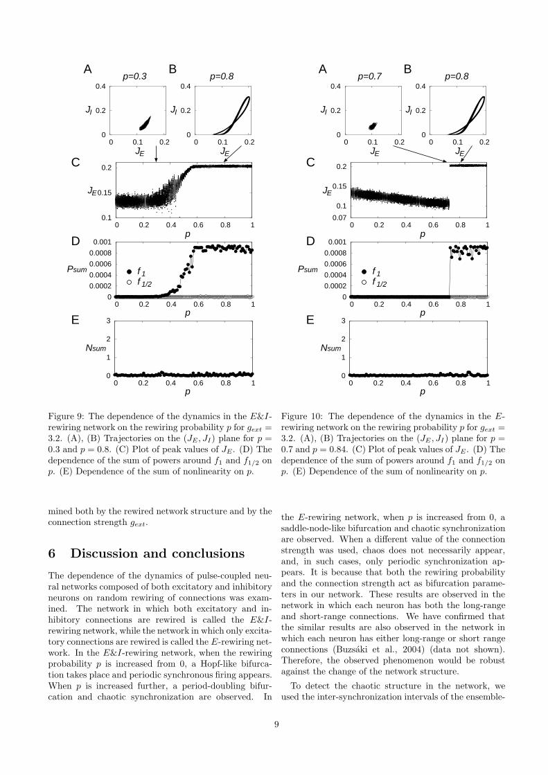
In this section, we set gext = 3.2, which is the valuemainly used in our previous study (Kanamaru & Ai-hara, 2010), and we observe the dynamics of the network.Figures 9 and 10 show the dependence of the dynamicson the rewiring probability p in the E&I-rewiring net-work and that in the E-rewiring network, respectively.

In each network, the power spectrum does not havea peak at f1/2 as shown in Figures 9D and 10D; there-fore, the period-doubling bifurcation does not take placewhen gext = 3.2 in these networks. Moreover, the sum ofnonlinearity fluctuates around zero as shown in Figures9E and 10E; therefore, chaotic dynamics is not observedin the time series obtained from these network.

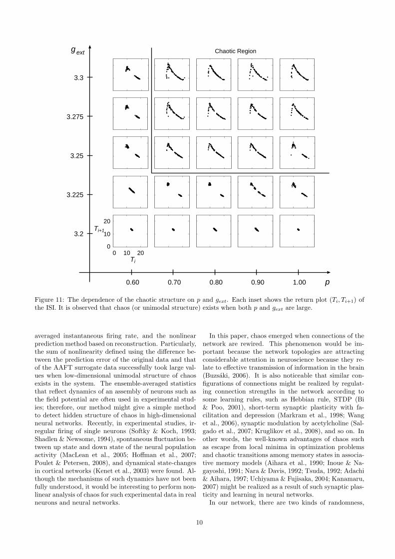
The reason for this difference of the dynamics is be-cause chaos in our network depends on both p and gext.Figure 11 shows the dependence of the chaotic structureon p and gext. Each inset shows the return plot (Ti, Ti+1)of the ISI (see also Figure 5). It is observed that chaos(or unimodal structure) exists when both p and gext arelarge. When p becomes large, the ISI Ti tends to becomelong (data not shown). On the other hand, when gext

becomes large, the ISI Ti tends to become short. There-fore, for large p and gext, a competition for the length ofISI takes place, then the period-doubling and generationof chaos will take place.

In summary, we found both the rewiring-inducedchaotic synchronization (Sections 3 and 4) and therewiring-induced periodic synchronization (Section 5).Those dynamical properties of the network are deter-

8

0

0.2

0.4

0 0.1 0.2 0

0.2

0.4

0 0.1 0.2

0

1

2

3

0 0.2 0.4 0.6 0.8 1

0

0.0002

0.0004

0.0006

0.0008

0.001

0 0.2 0.4 0.6 0.8 1

0.1

0.15

0.2

0 0.2 0.4 0.6 0.8 1

JE JE

JIJI

p=0.8p=0.3A B

C

JE

p

p

p

Psum

D

E

Nsum

f 1f 1/2

Figure 9: The dependence of the dynamics in the E&I-rewiring network on the rewiring probability p for gext =3.2. (A), (B) Trajectories on the (JE , JI) plane for p =0.3 and p = 0.8. (C) Plot of peak values of JE . (D) Thedependence of the sum of powers around f1 and f1/2 onp. (E) Dependence of the sum of nonlinearity on p.

mined both by the rewired network structure and by theconnection strength gext.

6 Discussion and conclusions

The dependence of the dynamics of pulse-coupled neu-ral networks composed of both excitatory and inhibitoryneurons on random rewiring of connections was exam-ined. The network in which both excitatory and in-hibitory connections are rewired is called the E&I-rewiring network, while the network in which only excita-tory connections are rewired is called the E-rewiring net-work. In the E&I-rewiring network, when the rewiringprobability p is increased from 0, a Hopf-like bifurca-tion takes place and periodic synchronous firing appears.When p is increased further, a period-doubling bifur-cation and chaotic synchronization are observed. In

0

0.0002

0.0004

0.0006

0.0008

0.001

0 0.2 0.4 0.6 0.8 1

0.07

0.1

0.15

0.2

0 0.2 0.4 0.6 0.8 1

0

1

2

3

0 0.2 0.4 0.6 0.8 1

0

0.2

0.4

0 0.1 0.2 0

0.2

0.4

0 0.1 0.2JE JE

JIJI

p=0.8p=0.7A B

C

JE

p

p

p

Psum

D

E

Nsum

f 1f 1/2

Figure 10: The dependence of the dynamics in the E-rewiring network on the rewiring probability p for gext =3.2. (A), (B) Trajectories on the (JE , JI) plane for p =0.7 and p = 0.84. (C) Plot of peak values of JE . (D) Thedependence of the sum of powers around f1 and f1/2 onp. (E) Dependence of the sum of nonlinearity on p.

the E-rewiring network, when p is increased from 0, asaddle-node-like bifurcation and chaotic synchronizationare observed. When a different value of the connectionstrength was used, chaos does not necessarily appear,and, in such cases, only periodic synchronization ap-pears. It is because that both the rewiring probabilityand the connection strength act as bifurcation parame-ters in our network. These results are observed in thenetwork in which each neuron has both the long-rangeand short-range connections. We have confirmed thatthe similar results are also observed in the network inwhich each neuron has either long-range or short rangeconnections (Buzsaki et al., 2004) (data not shown).Therefore, the observed phenomenon would be robustagainst the change of the network structure.

To detect the chaotic structure in the network, weused the inter-synchronization intervals of the ensemble-

9

p

Ti+1

Ti

10 200

10

20

0

0.60 0.70 0.80 0.90 1.00

3.3

3.275

3.25

3.225

3.2

gext Chaotic Region

Figure 11: The dependence of the chaotic structure on p and gext. Each inset shows the return plot (Ti, Ti+1) ofthe ISI. It is observed that chaos (or unimodal structure) exists when both p and gext are large.

averaged instantaneous firing rate, and the nonlinearprediction method based on reconstruction. Particularly,the sum of nonlinearity defined using the difference be-tween the prediction error of the original data and thatof the AAFT surrogate data successfully took large val-ues when low-dimensional unimodal structure of chaosexists in the system. The ensemble-averaged statisticsthat reflect dynamics of an assembly of neurons such asthe field potential are often used in experimental stud-ies; therefore, our method might give a simple methodto detect hidden structure of chaos in high-dimensionalneural networks. Recently, in experimental studies, ir-regular firing of single neurons (Softky & Koch, 1993;Shadlen & Newsome, 1994), spontaneous fluctuation be-tween up state and down state of the neural populationactivity (MacLean et al., 2005; Hoffman et al., 2007;Poulet & Petersen, 2008), and dynamical state-changesin cortical networks (Kenet et al., 2003) were found. Al-though the mechanisms of such dynamics have not beenfully understood, it would be interesting to perform non-linear analysis of chaos for such experimental data in realneurons and neural networks.

In this paper, chaos emerged when connections of thenetwork are rewired. This phenomenon would be im-portant because the network topologies are attractingconsiderable attention in neuroscience because they re-late to effective transmission of information in the brain(Buzsaki, 2006). It is also noticeable that similar con-figurations of connections might be realized by regulat-ing connection strengths in the network according tosome learning rules, such as Hebbian rule, STDP (Bi& Poo, 2001), short-term synaptic plasticity with fa-cilitation and depression (Markram et al., 1998; Wanget al., 2006), synaptic modulation by acetylcholine (Sal-gado et al., 2007; Kruglikov et al., 2008), and so on. Inother words, the well-known advantages of chaos suchas escape from local minima in optimization problemsand chaotic transitions among memory states in associa-tive memory models (Aihara et al., 1990; Inoue & Na-gayoshi, 1991; Nara & Davis, 1992; Tsuda, 1992; Adachi& Aihara, 1997; Uchiyama & Fujisaka, 2004; Kanamaru,2007) might be realized as a result of such synaptic plas-ticity and learning in neural networks.

In our network, there are two kinds of randomness,

10

namely, noise added to each neuron and random rewiringof connections. Both act as bifurcation parameters toyield chaotic synchronization, in which each neuron fluc-tuates because of noise, but the ensemble-averaged dy-namics can show deterministic chaos. This result sug-gests that rewiring-induced randomness in the systemdoes not necessarily contaminate the system, and some-times it even introduces rich dynamics to the system suchas chaos. It has already been known that the rewiringcan induce periodic or chaotic synchronization in somenetworks (Barahona & Pecora, 2002; Hong, Choi, &Kim, 2002; Hagberg & Schult, 2008), but the periodicor chaotic dynamics in such networks were determinedmainly by the dynamics of each element. In our model,chaos is a property of the rewired network because eachneuron has a stable equilibrium and shows neither peri-odic nor chaotic oscillation when it is disconnected fromthe other neurons.

Recently, it was reported that the existence of noisecan generate chaos in some nonlinear systems with mul-tiple elements (Kanamaru & Sekine, 2005b; Kanamaru,2006, 2007; Ichiki, Ito, & Shiino, 2007; Kanamaru &Aihara, 2008). In such systems, the behavior of each el-ement is noisy, but by averaging the dynamics of manyelements, chaos can emerge. Similarly, it is known thatchaos also emerges by introducing variability to somenonlinear systems such as cutting the connections in anassociative network (Nara & Davis, 1992), co-evolutionof phases and connection weights in coupled phase oscil-lators (Aoki & Aoyagi, 2009), and so on. The rewiring-induced chaos observed in the present paper would givea new possible scenario to generate chaos in neural sys-tems.

Acknowledgement

This research is partially supported by a Grant-in-Aid for Encouragement of Young Scientists (B)(No. 20700215), a Grant-in-Aid for Scientific Re-search on Priority Areas -System study on higher-orderbrain functions- from the Ministry of Education, Cul-ture, Sports, Science and Technology of Japan (No.17022012), and the Japan Society for the Promotionof Science (JSPS) through its “Funding Program forWorld-Leading Innovative R&D on Science and Tech-nology (FIRST Program).”

A Definition of the Network

A pulse-coupled neural network composed of excitatoryand inhibitory neurons arranged in a two-dimensionalarray is considered. An excitatory neuron and an in-hibitory neuron are placed at the point (i, j) (1 ≤ i ≤Nx, 1 ≤ j ≤ Ny) in the array, and both the numberof neurons in the excitatory ensemble and that in theinhibitory ensemble are NxNy. The dynamics of the in-ternal states θ

(i,j)E of the excitatory neuron as well as

θ(i,j)I of the inhibitory neuron at (i, j), is written as

τX˙

θ(i,j)X = (1 − cos θ

(i,j)X ) + (1 + cos θ

(i,j)X )

×(rX + ξ(i,j)X (t) + gXEI

(i,j)XE (t) − gXII

(i,j)XI (t)

+ggapδXII(i,j)gap (t)), (A.1)

I(i,j)XY (t) =

1

2#A(i,j)cXY

∑(m,n)∈A

(i,j)cXY

∑l

1κY

exp

(− t − t

(m,n)l

κY

), (A.2)

I(i,j)gap (t) =

1

#A(i,j)g

∑(m,n)∈A

(i,j)g

sin(θ(m,n)I (t) − θ

(i,j)I (t)

), (A.3)

〈ξ(i,j)X (t)ξ(m,n)

Y (t′)〉 = DδXY δimδjnδ(t − t′), (A.4)

where X = E or I, and δij is Kronecker’s delta (Er-mentrout, 1996; Izhikevich, 1999; Kanamaru & Aihara,2008). Each neuron is modeled by the theta neuron (Er-mentrout, 1996), which is known as a general model oftype-I neuron (Izhikevich, 1999); therefore, the dynam-ics of our network would also be observed in networksof other type-I neurons. Although the number of excita-tory neurons in the cortex is much larger than that of in-hibitory neurons, we set both the numbers to be identicalfor simplicity. As shown in equations A.2 and A.3, thesynaptic weights are divided by the number of connectedneurons; therefore, the dynamics of the network does notdepend on the number of neurons if there is a sufficientlylarge number of neurons. Connections through chemicalsynapses are modeled by the postsynaptic potential withan exponential function, and electrical synapses with gapjunctions based on physiological observations (Galarreta& Hestrin, 2001) are introduced to the connections be-tween the inhibitory neurons. Electrical synapses cor-respond to the diffusive coupling in physical systems;therefore, synchronization in the neural system can beinduced (Ermentrout, 2006). I

(i,j)XY denotes the inputs

by chemical synapses from the ensemble Y to the neu-ron at (i, j) in the ensemble X . A

(i,j)cXY denotes a set of

indices at which there is a neuron in the ensemble Y ,which connects to the neuron at (i, j) in the ensembleX . #A

(i,j)cXY is the number of elements of this set. t

(m,n)l

denotes the lth firing time of the neuron at (m, n) in theensemble Y and is defined by the time at which θ

(m,n)Y

exceeds π. I(i,j)gap (t) is the input by electrical synapses.

A(i,j)g denotes the set of indices at which there is a neu-

ron that connects to the target neuron through electricalsynapses. rX denotes the parameters of the neurons inensemble X . Without Gaussian white noise ξ

(i,j)X (t) and

input I(i,j)XY , a single neuron shows self-oscillation when

rX > 0. When rX < 0, on the other hand, this neuronbecomes an excitable system with the following stable

11

equilibrium:

θ0 = − arccos1 + rX

1 − rX, (A.5)

where θ0 approaches zero when rX → 0. In the liter-ature of synchronization in neural systems, many au-thors examined the synchronization of excitatory oscil-lators (Mirollo & Strogatz, 1990; Kuramoto, 1991; Ab-bott & van Vreeswijk, 1993; Tsodyks, Mitkov, & Som-polinsky, 1993; Hansel, Mato, & Meunier, 1995; vanVreeswijk, 1996; Sato & Shiino, 2002) or inhibitory os-cillators (van Vreeswijk, Abbott, & Ermentrout, 1994;Wang & Buzsaki, 1996; White et al., 1998; Golomb &Hansel, 2000; Lewis & Rinzel, 2003; Nomura, Fukai, &Aoyagi, 2003). However, in the present study, we setrE = rI = −0.025, and we consider the dynamics of net-works composed of excitable neurons only. Our neuronmodel stays on the stable equilibrium when the noiseintensity D is set to zero, irrespective of the values ofthe connections strength gXY and ggap because there isno firing. When D > 0 and gXY = ggap = 0, eachneuron in our network shows stochastic firing, which isneither periodic nor chaotic. When D > 0, gXY �= 0,and ggap �= 0, the firing of neurons in our network istypically asynchronous. However, when the values of D,gXY , and ggap are appropriately chosen and when thenetwork is sufficiently rewired as explained below, syn-chronous firing appears.

For simplicity, the parameters are set as gEE = gII ≡gint and gEI = gIE ≡ gext. The time constants of theinternal dynamics and the synaptic transmission are setto τE = 1, τI = 0.5, κE = 1, and κI = 5.

B Algorithm to obtain A(i,j)(p, k)

In this section, the algorithm to obtain the rewired con-nection A(i,j)(p, k) from the local connections A(i,j)(0, k)is explained. From N#A(i,j)(0, k) connections in thenetwork of N neurons, Np#A(i,j)(0, k) connections areselected randomly (N = NE = NI). Let us assumethat the connection from the neuron at (s, t) to thatat (i, j) is selected, i.e., (s, t) ∈ A(i,j)(0, k). After se-lecting a new neuron at (u, v) that is not included inA(i,j)(0, k) randomly, (s, t) is removed from A(i,j)(0, k)and (u, v) is added to A(i,j)(0, k). Then, in order tokeep the symmetric connections, (i, j) is removed fromA(s,t)(0, k) and added to A(u,v)(0, k). With this pro-cedure, a set A(i,j)(p, k) of rewired connections to theneuron at (i, j) is obtained.

C Definition of L(p) and C(p)

In this section we define the average shortest path lengthL(p) and the clustering coefficient C(p).

The shortest path length between two neurons is theminimum number of synapses to pass for one neuronto reach to another one, and by averaging it over thenetwork, L(p) is obtained.

Next, to define C(p), we define the local clusteringcoefficient Ci(p). We count the number ei of pairs ofinter-connected neurons which also are connected to theith neuron. Using the number ki of neurons that connectto the ith neuron, Ci(p) is defined as

Ci(p) =2ei

ki(ki − 1). (C.1)

By averaging Ci(p) over all the neurons, C(p) is ob-tained.

D Nonlinear prediction based onreconstruction

In this section, the nonlinear prediction method basedon reconstruction of dynamics is summarized (Theiler etal., 1992; Sauer, 1994; Suzuki, et al., 2000; Shinoharaet al., 2002; Kanamaru & Sekine, 2005a; Hirata et al.,2008). With the kth peak time tk of the firing rate of anexcitatory ensemble, the inter-synchronization interval(ISI) is defined as

Tk = tk+1 − tk. (D.1)

Let us consider an ISI sequence {Tk} and the delay co-ordinate vectors Vj = (Tj−m+1, Tj−m+2, . . . , Tj) withthe reconstruction dimension m, and let L be the num-ber of vectors in the reconstructed phase space Rm.For a fixed integer j0, we choose l = βL (β < 1)points that are nearest to the point Vj0 and denote themby Vjk

= (Tjk−m+1, Tjk−m+2, . . . , Tjk)(k = 1, 2, . . . , l).

With {Vjk}, a predictor of Tj0 for h steps ahead is de-

fined as

pj0(h) =1l

l∑k=1

Tjk+h. (D.2)

With pj0(h), the normalized prediction error (NPE) isdefined as

ENP (h) =〈(pj0 (h) − Tj0+h)2〉1/2

〈(〈Tj0〉 − Tj0+h)2〉1/2, (D.3)

where 〈·〉 denotes the average over j0. When the em-bedded vector Vj has structure such as a strange attrac-tor, we say that the system has deterministic structure.Note that a periodic solution where the firing rate ofthe network oscillates with an average interval T is re-garded as a stochastic process around T ; hence it doesnot have deterministic structure. A small value of NPEi.e., less than 1, implies that the ISI sequence has de-terministic structure behind the time series because thisalgorithm is based on the assumption that the dynami-cal structure of a finite-dimensional deterministic systemcan be well reconstructed by the delay coordinates of ISI(Sauer, 1994). However, stochastic time series with largeauto-correlations can also take NPE values less than 1.Therefore, we could not conclude that there is determin-istic structure only from the magnitude of NPE.

12

To confirm the deterministic structure, the values ofNPE should be compared with those of NPE for a setof surrogate data (Theiler et al., 1992). The surrogatedata are new time series generated from the originaltime series under some null hypotheses so that the newtime series preserve some statistical properties of theoriginal data. In the present study we use two kindsof surrogates, namely, random shuffled (RS) and am-plitude adjusted Fourier transformed (AAFT) surrogatedata which correspond to the null hypothesis of an in-dependent and identically distributed random processand that of a linear stochastic process observed througha monotonic nonlinear function, respectively. To makeAAFT surrogate data, we used TISEAN 3.0.1 (Hegger,Kantz, & Schreiber, 1999; Schreiber & Schmitz, 2000). Ifthe values of NPE for the original data are significantlysmaller than those of NPE for the surrogate data, thenull hypothesis is rejected, and it can be concluded thatthere is some possibility that the original time series hasdeterministic structure.

ReferencesAbbott, L. F., & van Vreeswijk, C. (1993).Asynchronous states in networks of pulse-coupledoscillators. Phys. Rev. E, 48, 1483–1490.

Adachi, M., & Aihara, K. (1997). Associative dynamicsin a chaotic neural network. Neural Networks, 10,83–98.

Aihara, K., Matsumoto, G., & Ikegaya, Y. (1984).Periodic and non-periodic responses of a periodicallyforced Hodgkin-Huxley oscillator, J. Theor. Biol., 109,249–269.

Aihara, K., Numajiri, T., Matsumoto, G., & Kotani,M. (1986). Structures of attractors in periodicallyforced neural oscillators. Phys. Lett. A, 116, 313–317.

Aihara, K., Takabe, T., & Toyoda, M. (1990). Chaoticneural networks. Physics Letters A, 144, 333–340.

Aihara, K., & Tokuda, I. (2002). Possible neural codingwith interevent intervals of synchronous firing. Phys.Rev. E, 66, 026212.

Aoki, T., & Aoyagi, T. (2009). Co-evolution of phasesand connection strengths in a network of phaseoscillators. Phys. Rev. Lett., 102, 034101.

Barahona, M., & Pecora, L. M. (2002). Synchronizationin small-world systems. Phys. Rev. Lett., 89, 054101.

Bi, G. & Poo, M. (2001). Synaptic modification bycorrelated activity: Hebb’s postulate revisited. Annu.

Rev. Neurosci. 24, 139–166.

Brunel, N. (2000). Dynamics of sparsely connectednetworks of excitatory and inhibitory spiking neurons.J. Comput. Neurosci., 8, 183–208.

Buzsaki, G. (2006). Rhythms of the brain. New York:Oxford University Press.

Buzsaki, G., Geisler, C., Henze, D. A., & Wang, X.-J.(2004). Interneuron diversity series: Circuit complexityand axon wiring economy of cortical interneurons.Trends Neurosci., 27, 186–193.

Ermentrout, B. (1996). Type I membranes, phaseresetting curves, and synchrony. Neural Comput., 8,979–1001.

Ermentrout, B. (2006). Gap junctions destroypersistent states in excitatory networks. Phys. Rev. E,74, 031918.

Feudel, U., Neiman, A., Pei, X., Wojtenek, W., Braun,H., Huber, M., & Moss, F. (2000). Homoclinicbifurcation in a Hodgkin-Huxley model of thermallysensitive neurons. Chaos, 10, 231–239.

Freeman, W. J. (1987). Simulation of chaotic EEGpatterns with a dynamic model of the olfactory system.Biol. Cybern. 56, 139–150.

Galarreta, M., & Hestrin, S. (2001). Electrical synapsesbetween GABA-releasing interneurons. Nature Rev.Neurosci., 2, 425–433.

Golomb, D., & Hansel, D. (2000). The number ofsynaptic inputs and the synchrony of large, sparseneuronal networks, Neural Comput., 12, 1095–1139.

Hagberg, A., & Schult, D. A. (2008). Rewiringnetworks for synchronization. Chaos, 18, 037105.

Hansel, D., Mato, G., & Meunier, C. (1995). Synchronyin excitatory neural networks. Neural Comput., 7,307–337.

Hayashi, H., Ishizuka, S., Ohta, M., & Hirakawa, K.(1982). Chaotic behavior in the onchidium giantneuron under sinusoidal stimulation. Phys. Lett., 88A,435–438.

Hegger, R., Kantz, H., & Schreiber, T. (1999).Practical implementation of nonlinear time series

13

methods: The TISEAN package. Chaos, 9, 413–435.

Hirata, Y., Katori, Y., Shimokawa, H., Suzuki, H.,Blenkinsop, T.A., Lang, E.J., Aihara, K. (2008).Testing a neural coding hypothesis using surrogatedata. Journal of Neuroscience Methods, 172, 312–322.

Hoffman, K.L., Battaglia, F.P., Harris, K., MacLean,J.N., Marshall, L., & Mehta, M.R. (2007). The upshotof Up states in the neocortex: From slow oscillations tomemory formation. J. Neurosci., 27, 11838–11841.

Hong, H., Choi, M. Y., & Kim, B. J. (2002).Synchronization on small-world networks. Phys. Rev.E, 65, 026139.

Ichiki, A., Ito, H., & Shiino, M. (2007).Chaos-nonchaos phase transitions induced bymultiplicative noise in ensembles of coupledtwo-dimensional oscillators. Physica E, 40, 402–405.

Inoue, M., & Nagayoshi, A. (1991). A chaosneuro-computer. Physics Letters A, 158, 373–376.

Izhikevich, E. M. (1999). Class 1 neural excitability,conventional synapses, weakly connected networks, andmathematical foundations of pulse-coupled models.IEEE Trans. Neural Networks, 10, 499–507.

Kanamaru, T. (2006). Blowout bifurcation and on-offintermittency in pulse neural networks with multiplemodules. International Journal of Bifurcation andChaos, 16, 3309–3321.

Kanamaru, T. (2007). Chaotic pattern transitions inpulse neural networks. Neural Networks, 20, 781–790.

Kanamaru, T., & Aihara, K. (2008). Stochasticsynchrony of chaos in a pulse-coupled neural networkwith both chemical and electrical synapses amonginhibitory neurons. Neural Comput., 20, 1951–1972.

Kanamaru, T., & Aihara, K. (2010). Roles ofinhibitory neurons in rewiring-induced synchronizationin pulse-coupled neural networks. Neural Comput., 22,1383–1398.

Kanamaru, T., & Sekine, M. (2005a). Detecting chaoticstructures in noisy pulse trains based on interspikeinterval reconstruction. Biol. Cybern., 92, 333–338.

Kanamaru, T., & Sekine, M. (2005b). Synchronizedfirings in the networks of class 1 excitable neurons withexcitatory and inhibitory connections and theirdependences on the forms of interactions. Neural

Comput., 17, 1315–1338.

Kenet, T., Bibitchkov, D., Tsodyks, M., Grinvald, A.,& Arieli, A. (2003). Spontaneously emerging corticalrepresentations of visual attributes, Nature 425,954–956.

Kitano, K., & Fukai, T. (2007). Variability v.s.synchronicity of neuronal activity in local corticalnetwork models with different wiring topologies. J.Comput. Neurosci., 23, 237–250.

Kruglikov, I. & Rudy, B. (2008). Perisomatic GABArelease and thalamocortical integration onto neocorticalexcitatory cells are regulated by neuromodulators.Neuron, 58, 911–924.

Kuramoto, Y. (1991). Collective synchronization ofpulse-coupled oscillators and excitable units. PhysicaD, 50, 15–30.

Lago-Fernandez, L. F., Huerta, R., Corbacho, F., &Siguenza, J. A. (2000). Fast response and temporalcoherent oscillations in small-world networks. Phys.Rev. Lett., 84, 2758–2761.

Lewis, T. J., & Rinzel, J. (2003). Dynamics of spikingneurons connected by both inhibitory and electricalcoupling. J. Comput. Neurosci., 14, 283–309.

MacLean, J.N., Watson, B.O., Aaron, G.B., & Yuste,R. (2005). Internal dynamics determine the corticalresponse to thalamic stimulation. Neuron, 48, 811–823.

Markram, H., Wang, Y., & Tsodyks, M. (1998).Differential signaling via the same axon of neocorticalpyramidal neurons. Proc. Natl. Acad. Sci. USA, 95,5323–5328.

Masuda, N., & Aihara, K. (2004). Global and localsynchrony of coupled neurons in small-world networks.Biol. Cybern., 90, 302–309.

Matsumoto, G., Aihara, K., Ichikawa, M., & Tasaki, A.(1984). Periodic and nonperiodic responses ofmembrane potentials in squid giant axons duringsinusoidal current stimulation. J. Theoret. Neurobiol.3, 1–14.

Mirollo, R. E., & Strogatz, S. H. (1990).Synchronization of pulse-coupled biological oscillators.SIAM J. Appl. Math., 50, 1645–1662.

Munro, E., & Borgers, C. (2010). Mechanisms of veryfast oscillations in networks of axons coupled by gap

14

junctions. J. Comput. Neurosci., 28, 539–555.

Nara, S., & Davis, P. (1992). Chaotic wandering andsearch in a cycle-memory neural network. Progress ofTheoretical Physics, 88, 845–855.

Netoff, T. I., Clewley, R., Arno., S., Keck, T., & White,J. A. (2004). Epilepsy in small-world networks. J.Neurosci., 24, 8075–8083.

Nomura, M., Fukai, T., & Aoyagi, T. (2003).Synchrony of fast-spiking interneurons interconnectedby GABAergic and electrical synapses. NeuralComput., 15, 2179–2198.

Ott, E. (1993). Chaos in Dynamical Systems.Cambridge University Press, New York.

Poulet, J.F.A., & Petersen, C.C.H. (2008). Internalbrain state regulates membrane potential synchrony inbarrel cortex of behaving mice. Nature, 454, 881–885.

Roxin, A., Riecke, H., & Solla, S. A. (2004).Self-sustained activity in a small-world network ofexcitable neurons. Phys. Rev. Lett., 92, 198101.

Salgado, H., Bellay, T., Nichols, J.A., Bose, M.,Martinolich, L., Perrotti, L., & Atzori, M. (2007).Muscarinic M2 and M1 receptors reduce GABA releaseby Ca2+ channel modulation through activation ofPI2K/Ca2+-independent and PLC/Ca2+-dependentPKC. Journal of Neurophysiology 98, 952–965.

Sato, Y. D., & Shiino, M. (2002). Spiking neuronmodels with excitatory or inhibitory synaptic couplingsand synchronization phenomena. Phys. Rev. E, 66,041903.

Sauer, T. (1994). Reconstruction of dynamical systemsfrom interspike interval. Rhys. Rev. Lett, 72,3811–3814.

Schreiber, T., & Schmitz, A. (2000). Surrogate timeseries. Physica D, 142, 346–382.

Shadlen, M. N., & Newsome, W.T. (1994). Noise,neural codes and cortical organization. Curr. Opin. inNeurobiol., 4, 569–579.

Shinohara, Y., Kanamaru, T., Suzuki, H., Horita, T., &Aihara, K. (2002). Array-enhanced coherence resonanceand forced dynamics in coupled FitzHugh-Nagumoneurons with noise. Phys. Rev. E, 65, 051906.

Softky, W.R., & Koch, C. (1993). The highly irregular

firing of cortical cells is inconsistent with temporalintegration of random EPSPs, J. Neurosci., 13,334–350.

Strogatz, S. H. (2001). Exploring complex networks.Nature, 410, 268–276.

Suzuki, H., Aihara, K., Murakami, J., & Shimozawa, T.(2000). Analysis of neural spike trains with interspikeinterval reconstruction. Biol. Cybern., 82, 305–311.

Theiler. J., Eubank. S., Longtin. A., Galdrikian. B., &Farmer. J.D. (1992). Testing for nonlinearity in timeseries: the method for surrogate data. Physica D, 58,77–94.

Traub, R.D., Schmitz, D., Jefferys, J.G.R., & Draguhn,A. (1999). High-frequency population oscillations arepredicted to occur in hippocampal pyramidal neuronalnetworks interconnected by axoaxonal gap junctions.Neuroscience, 92, 407–426.

Tsodyks, M., Mitkov, I., & Sompolinsky, H. (1993).Pattern of synchrony in inhomogeneous networks ofoscillators with pulse interactions. Phys. Rev. Lett., 71,1280–1283.

Tsuda, I. (1992). Dynamic link of memory – Chaoticmemory map in nonequilibrium neural networks.Neural Networks, 5, 313–326.

Tsuda, I., Fujii, H., Tadokoro, S., Yasuoka, T., &Yamaguti Y. (2004). Chaotic itinerancy as amechanism of irregular changes betweensynchronization and desynchronization in a neuralnetwork. J. Integr. Neurosci., 17, 159.

Uchiyama, S., & Fujisaka, H. (2004). Chaoticitinerancy in the oscillator neural network withoutLyapunov functions. Chaos, 14, 699–706.

Varona, P., Torres, J. J., Huerta, R., Abarbanel, H. D.I., & Rabinovich, M. I. (2001). Regularizationmechanisms of spiking-bursting neurons. NeuralNetworks, 14, 865–875.

van Vreeswijk, C. (1996). Partial synchronization inpopulations of pulse-coupled oscillators. Phys. Rev. E,54, 5522–5537.

van Vreeswijk, C., Abbott, L. F., & Ermentrout, G. B.(1994). When inhibition not excitation synchronizesneural firing. J. Comput. Neurosci., 1, 313–321.

van Vreeswijk, C., & Sompolinsky, H. (1996). Chaos inneuronal networks with balanced excitatory and

15

inhibitory activity. Science, 274, 1724–1726.

Wang, X.-J., & Buzsaki, G. (1996). Gamma oscillationsby synaptic inhibition in a hippocampal interneuronalnetwork. J. Neurosci., 16, 6402–6413.

Wang, Y., Markram, H., Goodman, P.H., Berger, T.K.,Ma, J. and Goldman-Rakic, P.S. (2006). Heterogeneityin the pyramidal network of the medial prefrontalcortex. Nature Neuroscience, 9, 534–542.

Watts, D. J., & Strogatz, S. H. (1998). Collectivedynamics of ‘small-world’ networks. Nature, 393,440–442.

White, J. A., Chow, C. C., Ritt, J., Soto-Trevino, C., &Kopell, N. (1998). Synchronization and oscillatorydynamics in heterogeneous, mutually inhibited neurons.J. Comput. Neurosci., 5, 5–16.

16